URBAN & RURAL RUNOFF ROUTING APPLICATION
147
URBAN & RURAL RUNOFF ROUTING APPLICATION GETTING STARTED MANUAL
Transcript of URBAN & RURAL RUNOFF ROUTING APPLICATION

URBAN & RURAL RUNOFF ROUTING APPLICATION
GETTING STARTED MANUAL

xprafts Getting Started Manual Version 2013
TUTORIAL 1: AN OVERVIEW OF XPRAFTS 1 1.1 Introduction 1 1.2 Origin of xprafts 2 1.3 Accessing Help 4 1.4 Contact Us 4 1.5 Graphical Interface 5 1.6 Technical Overview 5
TUTORIAL 2: BASICS OF XPRAFTS 16 2.1 Introduction 16 2.2 Network Terminology 17
TUTORIAL 3: INPUT VARIABLES 23 3.1 Percent Impervious on Various Slopes 23 3.2 Manning’s n values on Rural Catchments with Various Slopes 24 3.3 Manning’s n values in Urban Areas 24
TUTORIAL 4: CREATING A SIMPLE NETWORK 26 4.1 Simple Network Introduction 26 4.2 Loading the Program 26 4.3 Creating the Network 27 4.4 Naming the Network 30 4.5 Setting the Global Database Information 32 4.6 Job Control Data 37 4.7 Link Data 39 4.8 Sub-Catchment Data 40 4.9 Saving the File and Solving the Network 42 4.10 Reviewing Results 42 4.11 Exiting Program 43
TUTORIAL 5: LINKING TO EXTERNAL DATABASES 44 5.1 Introduction 44 5.2 Setting up the Model 44 5.3 Linking with External Database 44 5.4 Importing Global Data 51
TUTORIAL 6: SUBDIVISION - PRE DEVELOPMENT 55 6.1 Using a Template 55 6.2 Adding a Background Image and Zoom Tool 56 6.3 Creating Nodes 58 6.4 Creating Links 59 6.5 Creating Catchments 60 6.6 Initial/Continuing Rainfall Loss Model 64 6.7 Reviewing Rainfall Data 66 6.8 Solving Hydrographs 69 6.9 Reviewing Graphical Results 70 6.10 Tabular Results and Data Input (xp tables) 73
TUTORIAL 7: SUBDIVISION - POST DEVELOPMENT 75 7.1 Entering Nodes and Links for the Post Developed Site 75 7.2 Splitting Catchments into Pervious and Impervious subcatchments. 76 7.3 Optimizing Basin 81
TUTORIAL 8: RIVER EXAMPLE 89 8.1 River Example Introduction 89 8.2 Link and Node Data 89 8.3 Infiltration and Rainfall Data 91 8.4 Weighted Rainfall Data to Individual Sub-Catchments 95 8.5 Gauged Flow or Stage Data 97 8.6 xprafts Review Results 99
TUTORIAL 9: DETENTION BASIN VERSUS ON SITE DETENTION 101 9.1 Introduction 101

xprafts Getting Started Manual Version 2013
9.2 Pre-Subdivision 103 9.3 Post Subdivision 111 9.4 Community Pond (PostSubPond.xp) 114 9.5 Post Subdivision with OSDs 119
TUTORIAL 10: PMP ESTIMATION 125 10.1 Introduction 125 10.2 Create File from Template 127 10.3 Load Background Image and Catchment Extent 127 10.4 Creating Subcatchments 128 10.5 Create catchment collection points 129 10.6 Setting up Spatial Distribution for Short Duration PMP 132 10.7 Automated Storm Generation 134 10.8 Setting up GSDM Data for Shorter Duration Storms 137 10.9 Setting up GSAM Data for Longer Duration PMP 140 10.10 Setting up GTSMR Data for Longer Duration PMP 144 10.11 Analysis and Results 144

xprafts Getting Started Manual Page 1
Tutorial 1: An Overview of xprafts
1.1 Introduction
xprafts is a comprehensive software program to simulate runoff hydrographs at
defined points throughout a watershed based on a set of catchment characteristics and
specific rainfall events. As shown in the diagram below the watershed can be subdivided
into a number of sub-catchments from which runoff hydrographs are produced and routed
through any configuration of network storages, channels, and pipes to determine flood
mitigation options, drainage strategies, or hydraulic design data.
Hyd
rogr
aph
Mod
ule
Q1Q2
Q3
Pipe
#2
Q
Q1(t)
Q2(t)
Q3(t)
t
Q4
Q5Q6
Q9
Diversion Channel
#2
#1
Q10 #2
q(t)*L
Basin ModuleQ7
Q8 Q6(t)
t
Q
Q
t
Q4(t)
Q5(t)
Pipe/Floodway
Q8(t)
Q7(t)
Channel Modules
t
Q9(t)
Q10(t)q(t)*L
Q11
Q12
Q
t
Q12(t)
#1
#1
RI
t t
+ RP
Impervious Area Pervious Area
RI
t t
+ RP
Impervious Area Pervious Area
#2
#1 Initial & Continuing Rainfall
Losses
Philips’ Infiltration Losses
Rainfall Excess
Computed Hydrographs
Rainfall Input
Figure 1. 1 - Graphical Representation of xprafts
xprafts is suitable for application on catchments ranging from rural to fully urbanised.
There are no specific limitations on catchment size. xprafts has been successfully used
for catchments in excess of 20,000km2 including on-site detention. xprafts is capable
of analysing watersheds including natural waterways, formalised channels, or pipes,
retarding and retention basins and any combination of these.
xprafts Getting Started Manual Page 2
xprafts can be used to evaluate the effects of floods on major storage dams and the
effect of a dam break on watershed. It can also simulate the attenuating effects of channel
and floodplain storage on catchment runoff and assist the formulation of drainage
strategies on developed or developing catchments. xprafts can also be used to
facilitate flood forecasting and subsequent flood plain management activities. The model
allows rapid designs of networks with retarding/retention basins, giving great flexibility in
sizing outlets and emergency spillways to meet optimum requirements.
xprafts can be used as either an event-based model (design storms) or continuous
simulation model (historic time series rainfall data including the areal distribution over
watershed). When operating in either mode, the program has the option to utilise a water
balance model generating continuous excess rainfall. This water balance model is a
modified version of the Australian Representative Basins Model (Black & Aitken 1977,
Goyen 1981, Goyen 2000).
In summary xprafts may be used for any of the following tasks:
Evaluating catchment runoff peaks and volumes;
Sizing of hydraulic elements within a drainage system, including reservoirs and retarding basins, pipes, channels, floodways and river training works;
Examining of drainage and flood mitigation strategies;
Assessing the effects of various catchment changes, or urbanization, on runoff peaks and volumes;
Predicting flows for a flood warning system;
Estimating sewer flows; and
Generating hydrograph flows for hydraulic modeling in other software packages (i.e. xpstorm and xpswmm).
1.2 Origin of xprafts
The Rainfall/Runoff Routing Model described in this manual originated in 1974 in response
to the need of analysing a complex drainage system associated with a major development
in Darwin including a new town for about 150,000 persons.
The program was originally developed jointly by Willing & Partners Pty Ltd and the Snowy
Mountains Engineering Corporation (SMEC) (Goyen & Aitken 1976), and was named the
Regional Stormwater Drainage Model (RSWM).
The concept of the RSWM model followed intensive research in the early 1970s into existing
methods and computing rainfall/runoff models available in Australia and overseas including
Britain, France and the United States of America.
A number of technical investigations were undertaken, including local research, a study
tour by Mr. A.P. Aitken of SMEC (Aitken 1973), and a research project for the Australian

xprafts Getting Started Manual Page 3
Water Resources Council. Prior to the model being developed a number of research
activities concluded that no appropriate model consistent with Australian conditions and
data was available. This was particularly evident for urbanised and developing catchments.
The basic aim of the development of the RSWM program included the following:
Provide a deterministic model capable of handling any conceivable drainage or river system including natural and artificial storages;
Limit data input requirements to be consistent with the availability of data and the required accuracy of results;
Allow rapid engineering and economic assessment of alternative solutions to flooding and drainage problems. Since 1974 the RSWM model has been applied to studies throughout New South Wales, the Northern Territory, the Australian Capital Territory, Victoria, Papua New Guinea and Indonesia.
Watershed studies have ranged from rural to fully urban with catchment areas ranging
from less than 0.1 ha to several thousand square kilometers. The model has been improved
on a semi-continuous basis since 1974 and continues to be updated as results of ongoing
research is incorporated into the model structure. In the early 1980’s the program was
renamed the Runoff Analysis and Flow Training Simulation program (RAFTS). This was to
reflect the major shift to included detailed urban analysis during the period between 1983
and 1997.
The significant changes during the early 1980’s to the xprafts program are as below:
Separate consideration and routing of impervious and pervious sub areas within a sub-catchment. This procedure was found to greatly improve urban runoff parameter calibration;
Separate routing of pipes and channels in a floodway environment;
Major enhancements in the retarding basin module to include hydraulically interconnected basins, on-line and off-line basins with reverse flow considerations;
Substantial rewriting to make it compatible with micro-computer technology in terms of storage requirements and execution time;
Significant enhancements to the urban drainage capabilities of the program;
Improvements to the very large river basin simulation capabilities of the program.
In the 1980’s the custodianship of the programs development transferred from the general R&D within Willing and Partners Pty Ltd Consulting Engineers to XP Solutions (formerly XP Software), a dedicated development group acting independently of the consulting organisation.
Since 1997 the enhancements have continued and include:

xprafts Getting Started Manual Page 4
Water Sensitive Urban Design (WSUD) including advanced on-site detention and retention analysis, roof water tank consideration, and advancements in Flood Forecasting facilities;
Advances in sub-catchment analysis to provide improved scaling of process between sub-catchments of different sizes;
Automatic simulation of probable maximum precipitation (PMP); and
Major rewriting of the program to be fully Microsoft Windows compatible and work in full 32 bit operating code.
1.3 Accessing Help
The Help menu and Documentation are available for users and are easy to access. To
access Help information whilst using xprafts you can either make a selection from the
Help menu or simply click on the Help icon located on your toolbar. Some dialogs also
provide a Help option to specific information to that window. If you click on the Help icon
the pointer will turn into a question mark, then click on the area you require more
information about. If this is not active press key F1 while the dialog is open. This will
provide relevant help for all items in that dialog. Printed documentation is also available
from XP Solutions.
1.4 Contact Us
If you do experience difficulties when using our software please contact our technical
support team:
XP SOLUTIONS
Phone. +61-2-6253-1844
Fax. 61-2-6253-1847
PO Box 3064
Belconnen ACT 2617, Australia
Website: www.xpsolutions.com
Email: [email protected]
To improve your skills and increase productivity we would encourage you to attend our
training workshops that are organised on a regular basis. These workshops provide
comprehensive information to help you get the most out of our XP Solutions’ products.
Information regarding these workshops is regularly posted on our website. Alternatively
you can contact us using the email address or phone number as above. Should you need we
can also tailor our workshops to meet your particular requirements as well as organise in-
house training options.
xprafts Getting Started Manual Page 5
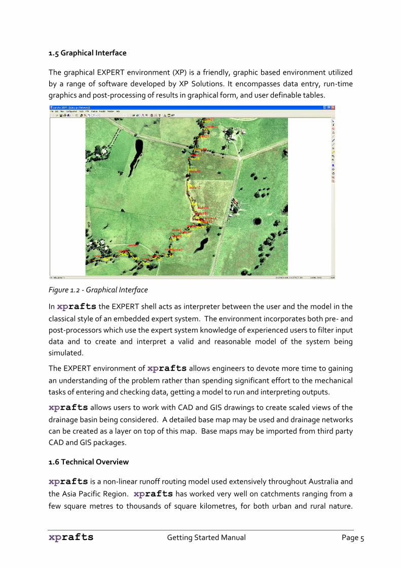
1.5 Graphical Interface
The graphical EXPERT environment (XP) is a friendly, graphic based environment utilized
by a range of software developed by XP Solutions. It encompasses data entry, run-time
graphics and post-processing of results in graphical form, and user definable tables.
Figure 1.2 - Graphical Interface
In xprafts the EXPERT shell acts as interpreter between the user and the model in the
classical style of an embedded expert system. The environment incorporates both pre- and
post-processors which use the expert system knowledge of experienced users to filter input
data and to create and interpret a valid and reasonable model of the system being
simulated.
The EXPERT environment of xprafts allows engineers to devote more time to gaining
an understanding of the problem rather than spending significant effort to the mechanical
tasks of entering and checking data, getting a model to run and interpreting outputs.
xprafts allows users to work with CAD and GIS drawings to create scaled views of the
drainage basin being considered. A detailed base map may be used and drainage networks
can be created as a layer on top of this map. Base maps may be imported from third party
CAD and GIS packages.
1.6 Technical Overview
xprafts is a non-linear runoff routing model used extensively throughout Australia and
the Asia Pacific Region. xprafts has worked very well on catchments ranging from a
few square metres to thousands of square kilometres, for both urban and rural nature.

xprafts Getting Started Manual Page 6
xprafts can model up to 10,000 different nodes and each node can have any size sub-
catchment attached as well as a storage basin. Additionally multiple on-site detention or
retention structures, within a sub-catchment, can be included in the analysis.
xprafts uses the Laurenson non-linear runoff routing procedure to develop a sub-
catchment stormwater runoff hydrograph from either an actual event (recorded rainfall
time series) or design storm using Intensity-Frequency-Duration (IFD) data together with
dimensionless storm temporal patterns as well as standard AR&R 1987 data. From the
2009 version onwards xprafts simulates Probable Maximum Precipitation (PMP).
Three loss models may be employed to generate excess rainfall. They are:
Initial/Continuing loss;
Initial/Proportional loss; and
ARBM full water balance model.
A reservoir routing model allows routing of inflow hydrographs through a user-defined
storage using the level pool routing procedure and allows modelling of hydraulically
interconnected basins and on-site detention facilities.
Three levels of hydraulic routing are available within xprafts:
Simple hydrograph lagging in pipes and channels;
Muskingum method;
Muskingum-Cunge procedure to route hydrographs though channel or river reaches; and
The hydrographs may be transferred to the xpswmm/xpstorm hydraulic simulation
program for detailed hydraulic analysis.
Hydrograph Generation: The Laurenson runoff routing procedure is used in xprafts
for the following reasons:
it offers a flexible model to simulate both rural and urban catchments;
it allows for non-linear response from catchments over a large range of event magnitudes;
it considers time-area and sub-catchment shape, and
it offers an efficient mathematical procedure for developing both rural, urban and mixed runoff hydrographs at any sub-catchment outlet.
Data requirements for xprafts consist of: catchment area, slope, degree of
urbanisation (derived from the nominated fraction impervious area), losses (observed or
design) and rainfall data.
These parameters are used to compute the storage delay coefficient for each sub-
catchment to develop the non-linear runoff hydrograph. A default exponent is adopted
although the user may specify this value with either a different non-linear exponent or

xprafts Getting Started Manual Page 7
rating table of flow vs. exponent to define different degrees of catchment non-linear
response.
Each sub-catchment is, by default, divided into 10 equal sub-areas as shown in Figure 1.3.
Each sub-area is treated as a cascading non-linear storage following the relationship
S , where n by default is set to – 0.285 and b is computed from observed catchment
event data or specified in terms of catchment parameters. The rainfall is applied to each
sub-area, and the rainfall excess is computed and converted into an instantaneous inflow.
This instantaneous flow is then routed through the sub-area storages to develop individual
sub-catchment outlet hydrograph. Figure 1.4 shows a diagram for the process.
10
1
2
34
56
78 9
A
1.00.9
0.8
0.70.6 0.5 0.4
0.30.2
0.1
P1
P2P3
P4 P5P6
P7P8
P9
P10
K1
K2
K3K4
K5K6
K7
K8
K9
K10
Catchment boundary
Isochrone
APluviograph
5 Subarea number
K2 Subarea concentrated storage
P7 Subarea total rainfall
Figure 1.3 - Subarea Definition

xprafts Getting Started Manual Page 8
Su
ba
rea
1S
ub
are
a 2
Pluviograph A
Pluviograph A
Ra
infa
ll In
ten
sity
Exce
ss R
ain
fall
Inte
nsity
Exce
ss R
ain
fall
Inte
nsity
Insta
nta
ne
ou
s In
flo
wIn
sta
nta
ne
ou
s In
flo
w
Subarea excess
rainfall
Subarea excess
rainfall
Instantaneous
Subarea Inflow
Instantaneous
Subarea Inflow
Routing through
non-linear
subarea storage
Routing through
non-linear
subarea storage
Outflow from
subarea 1
Outflow from
subarea 2
Ou
tflo
wO
utflo
w
Time
Time
S=k1(q)*q
S=k2(q)*q
S=volume of storage (hrs*cumecs)
q=instantaneous rate of runoff (cumecs)
k(q)=storage delay time as a function of q (hrs)
Loss model
Loss model
Figure 1.4 - Diagrammatic Representation of Hydrograph Generation
Figure 1.5 - Storm Data
Rainfall: Any local Intensity-Frequency-Duration (IFD) information may be used to
generate hydrographs. Rainfall input can be of two types, either Design Rainfall or Historic
Rainfall. Design rainfall may be entered as a dimensionless temporal pattern with average
rainfall intensity. In Australia design rainfall patterns may be input from AR&R 1987, with
intensity information derived from Volume 2 of AR&R 1987. In this way the appropriate
intensity for the given ARI and duration is computed automatically. The zone of different

xprafts Getting Started Manual Page 9
regions of Australia may be entered and the appropriate temporal pattern can also be
automatically identified from the inbuilt standard temporal patterns from AR&R 1987.
Historical events may be entered either in fixed or variable time steps allowing long periods
of recorded data to be defined efficiently. Alternatively, rainfall data can be read from an
external rainfall file in ASCII text format either in HYDSYS or XPX formats.
Loss Models: The rainfall excess can be computed using either of the following methods:
Initial/Continuing: The initial depth of rainfall loss is specified along with a continuing rate of loss. For example, 15mm initial loss plus 2.5 mm/hr of any further rainfall.
Initial/Proportional: The initial depth of rainfall loss is specified along with a proportion of any further rain that will be lost. For example, 15mm initial and 0.6 times any further rainfall.
ARBM Loss method: Infiltration parameters to suit the Philip’s infiltration equation using comprehensive ARBM algorithms are used to simulate catchment infiltration and subsequent rainfall excess for a particular rainfall sequence and catchment antecedent conditions.
Figure 1.6 - Hydrologic Losses
xprafts Getting Started Manual Page 10
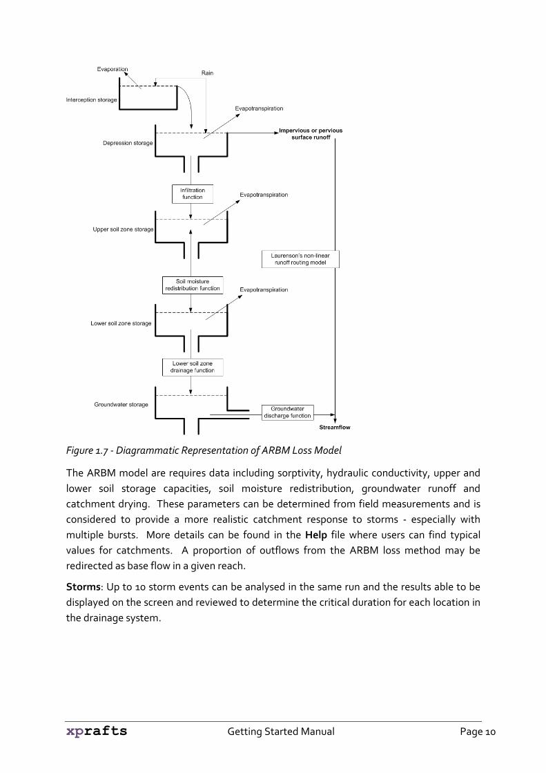
Figure 1.7 - Diagrammatic Representation of ARBM Loss Model
The ARBM model are requires data including sorptivity, hydraulic conductivity, upper and
lower soil storage capacities, soil moisture redistribution, groundwater runoff and
catchment drying. These parameters can be determined from field measurements and is
considered to provide a more realistic catchment response to storms - especially with
multiple bursts. More details can be found in the Help file where users can find typical
values for catchments. A proportion of outflows from the ARBM loss method may be
redirected as base flow in a given reach.
Storms: Up to 10 storm events can be analysed in the same run and the results able to be
displayed on the screen and reviewed to determine the critical duration for each location in
the drainage system.

xprafts Getting Started Manual Page 11
Figure 1.8 – Stacked Storms Dialog
Simulation runs of any period of time, from minutes to years, can be accommodated.
Weighting of different Rainfall Stations in individual sub-catchments is provided.
Figure 1.9 - Catchment Storms

xprafts Getting Started Manual Page 12
Gauged Data: Gauged Data may be entered by users or read directly from an external file
and compared to the computed hydrograph for to assist the calibration and verification of
the drainage network simulation.
Hydraulics: Hydrographs, which have been developed at individual nodes may be
transported through the drainage system in three ways:
Translation (Lagging): Users specify length of travel time from one node to the next and the hydrograph is translated on the time base by this length of time with no attenuation of peak flow. Appropriate values may be derived by estimating the velocity of flow and consequently the wave celerity, and knowing the length of travel.
Pipe Flow: A pipe may be specified (or sized) to carry flows. Any flows that exceed the capacity of the pipe will travel via the surface to either of two destination nodes. The travel time in this pipe may be either computed or set to a fixed number of minutes.
Channel Routing: A Channel/Stream may be defined using either compound trapezoidal channel or HEC2 style arbitrary sections. The cross-section shape may be imported directly from an existing HEC2 file. The Muskingum-Cunge method is used to route the flow through the channel with the consequent attenuation of the peak flow and delay of the hydrograph peak. Alternatively the detailed channel data simple Muskingum K & X parameters may be utilised.
Figure 1. 10 - Channel Routing

xprafts Getting Started Manual Page 13
Note: Any nodes may have a diversion link defined in addition to the normal link that will divert some or all of the flow and delay of the hydrograph peak.
The hydrographs generated in xprafts can be transferred to the xpswmm /
xpstorm hydrodynamic models. Hydrographs may also be read into other xprafts
models. For detailed description of xpswmm and xpstorm see separate xpswmm and
xpstorm technical descriptions on our website: www.xpsolutions.com.
Storage Basins (On-Site Detention, Ponds, Dams, etc.): Any nodes in xprafts may
be defined as a storage node. This storage can be small as few cubic meters or large as a
few millions cubic meters. On-line and off-line storages can be simulated and the storages
can be hydraulically interconnected.
Puls’ level pool routing technique is used to route the inflow hydrograph through the
nominated storages. A stage/storage relationship is defined for each storage.
Figure 1.11 - Retarding Basin
Different outlet structures can be modelled including:
circular pipe culverts;
rectangular box culverts;
broad crested weirs;
sharp crested weirs;
ogee weirs;
xprafts Getting Started Manual Page 14
erodible weirs;
multi-level weirs;
high level outlets;
rating curve outlets;
evaporation; and
infiltration.
Optimization methods are also available to help design the basin. You may optimize the
basin for a maximum discharge or for a maximum allowable storage.
Importing Data: Data may be imported from an ASCII text file in the XPX file format. This
format allows users to create new data and objects as well as update and add to existing
xprafts networks. This facility may be used to import information from GIS’s, FIS’s
CAD packages and other databases. Additionally, data may be directly imported from any
ODBC compliant database including Excel, DFF Dbase, etc. Plan drawings may be
imported from virtually any CAD or GIS packages to be used as a scaled base map. Formats
accepted include BMPs, Shape files, JPEG, DWG, DXF etc.
Output: xprafts provides results and data in various forms. All graphical displays may
be output to printers, plotters and to DXF files.
Graphical Output: xprafts provides graphs of rainfall, rainfall excess, and hydrographs
including total and local components of hydrographs. Stage history and storage history are
also available for any pond or basin in the drainage system. The graphs of multiple
locations may be displayed and printed or results exported to a comma delimited ASCII text
file for use in spreadsheets or databases.
xprafts Getting Started Manual Page 15
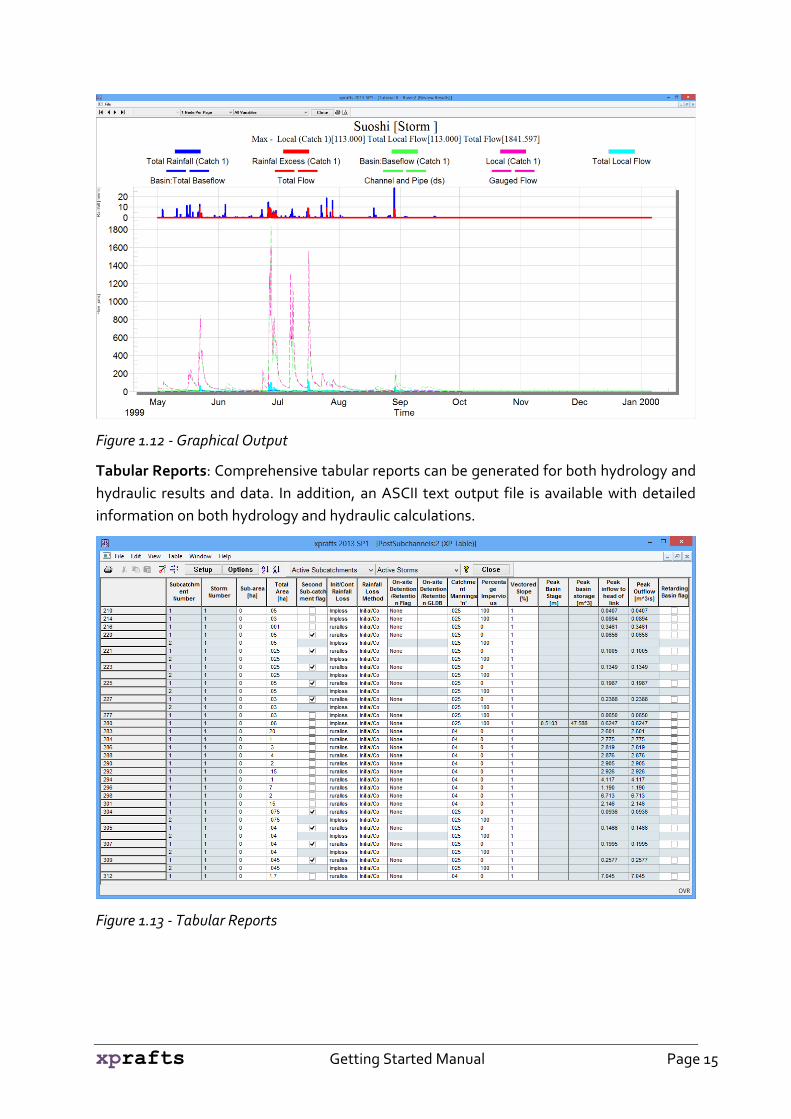
Figure 1.12 - Graphical Output
Tabular Reports: Comprehensive tabular reports can be generated for both hydrology and
hydraulic results and data. In addition, an ASCII text output file is available with detailed
information on both hydrology and hydraulic calculations.
Figure 1.13 - Tabular Reports

xprafts Getting Started Manual Page 16
Tutorial 2: Basics of xprafts
2.1 Introduction
xprafts models are built to represent the channel/pipe network within an urban, rural,
or partly urban catchment. Figure 1.1 in the Tutorial 1 diagrammatically describes a typical
catchment and channel/pipe network. The network is made up of links with a node at each
end. Each node is at the downstream end of a sub-catchment that collects local inflows.
The minimum number of nodes required to represent a catchment network is one and
located at the catchment outlet. In this case the node sub-catchment’s area is equal to the
complete catchment. Sub-catchments can be optionally split into two portions: usually
representing separate pervious and impervious areas within an urban sub-catchment.
Storm infiltration can be represented by simple initial continuous loss estimates or
infiltration determined using a comprehensive soil water balance module.
Nodes can contain the definition of a retarding basin. Individual sub-catchments can also
contain multiple water sensitive urban design storage structures including on site detention
and retention facilities.
Computed hydrographs, based on an input storm of any durations, are estimated at each
defined node. Additionally, channel routing estimates velocity, normal depth and storage
hydrograph attenuation.

xprafts Getting Started Manual Page 17
2.2 Network Terminology
1
4
79
1.01
2.01
1.02
3.01
1.03
1.04
Reservoir or retarding
basin
1.05
Main
chan
nel o
r river
Node Point (defining location of
hydrograph)
Isochrones
3.01 Link number
Watercourse
Sub-catchment Boundary
7 Subarea
For clarity, isochrones are shown
only in this subcatchment
Figure 2.1 - Network Terminology
As indicated in section 1.6 each sub-catchment is divided into ten (10) sub-areas (called
isochronal sub areas). These areas are based on equal times of travel to the sub-catchment
outlet. Any sub-catchments can contain distributed water sensitive urban design structures
such as on-site detention tanks/ponds, roof water tanks and/or infiltration/evaporation
structures.
xprafts Getting Started Manual Page 18
Link A
Link B
Local sub-catchment X
Local
sub-catchment Y
Top subcatchment slope
(X) for link AIntermediate
subcatchment slope (X) for
link B
Alternate subcatchment
slope (X) for link B
Main channel slope AB for
link A
Slope of subcatchment Y
is defined as average
slope based on a range of
alternate weighted
catchment slope
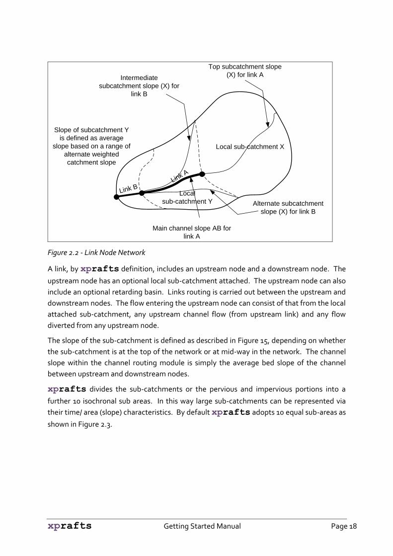
Figure 2.2 - Link Node Network
A link, by xprafts definition, includes an upstream node and a downstream node. The
upstream node has an optional local sub-catchment attached. The upstream node can also
include an optional retarding basin. Links routing is carried out between the upstream and
downstream nodes. The flow entering the upstream node can consist of that from the local
attached sub-catchment, any upstream channel flow (from upstream link) and any flow
diverted from any upstream node.
The slope of the sub-catchment is defined as described in Figure 15, depending on whether
the sub-catchment is at the top of the network or at mid-way in the network. The channel
slope within the channel routing module is simply the average bed slope of the channel
between upstream and downstream nodes.
xprafts divides the sub-catchments or the pervious and impervious portions into a
further 10 isochronal sub areas. In this way large sub-catchments can be represented via
their time/ area (slope) characteristics. By default xprafts adopts 10 equal sub-areas as
shown in Figure 2.3.

xprafts Getting Started Manual Page 19
10
1
2
34
56
78 9
A
1.00.9
0.8
0.70.6 0.5 0.4
0.30.2
0.1
P1
P2P3
P4 P5P6
P7P8
P9
P10
K1
K2
K3K4
K5K6
K7
K8
K9
K10
Catchment boundary
Isochrone
APluviograph
5 Subarea number
K2 Subarea concentrated storage
P7 Subarea total rainfall
Figure 2.3 – Isochrones
Retarding Basins/Detention Basins are represented in xprafts by defined stage/storage
and stage/discharge curves. A retarding basin can optionally occur at any node in network.
The stage/discharge curve can be internally estimated using defined outlet structure
characteristics.
When two storage structures interact hydraulically during a storm event xprafts
automatically accounts for the varying stage discharge characteristics based on the relative
levels in each basin.

xprafts Getting Started Manual Page 20
Figure 2.4 - Retarding Basin
A range of spillway conditions are available within a basin including standard weirs,
collapsible weirs as indicated in diagram and direct stage/ discharge routing and curves.
xprafts Getting Started Manual Page 21
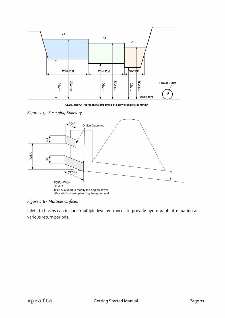
Figure 2.5 - Fuse plug Spillway
Figure 2.6 - Multiple Orifices
Inlets to basins can include multiple level entrances to provide hydrograph attenuation at
various return periods.

xprafts Getting Started Manual Page 22
Figure 2.7 - Floodway
Channel Routing can be based on simple lagging of hydrographs between the link’s
upstream and downstream node or Muskingum routing directly inputing K and X values or
Muskingum-Cunge routing that automatically computes K and X values based on input
channel x-sections and longitudinal characteristics.

xprafts Getting Started Manual Page 23
Tutorial 3: Input Variables
The shape of the hydrograph is influenced by the following variables:
Area
Slope
Roughness
Urbanisation (expressed as percentage impervious)
Rainfall loss model
The values shown in the following charts use the rainfall intensities and patterns for Cairns,
in north Queensland. They are used to show the general behaviour of the model. Consider
creating similar curves using the temporal patterns for your project area.
3.1 Percent Impervious on Various Slopes
Flat slopes are more affected by changes in percentage of Impervious area.
- 0.050 0.100 0.150 0.200 0.250 0.300 0.350 0.400 0.450 0.500
0 20 40 60 80 100 120Pe
ak
Flo
w/h
a (
m3
/s/h
a)
'
Percentage Impervious [%]
1 ha catchment with n = 0.025
s=0.01%
s=0.1%
s=1%
0
0.1
0.2
0.3
0.4
0.5
0.6
0 20 40 60 80 100 120Pe
ak
Flo
w/h
a (
m3
/s/h
a)
'
Percentage Impervious [%]
1 ha catchment with n = 0.025
s=5.%
s=10.%
s=15.%

xprafts Getting Started Manual Page 24
3.2 Manning’s n values on Rural Catchments with Various Slopes
Manning’s n values on rural catchments can have a significant effect on peak flows.
3.3 Manning’s n values in Urban Areas
Manning’s n values in highly urbanized areas have less effect as the slope is greater than
1%.
0
0.05
0.1
0.15
0.2
0.25
0.3
0.35
0 0.01 0.02 0.03 0.04 0.05 0.06Pe
ak
Flo
w/h
a (
m3
/s/h
a)
'
n value
1 ha catchment with 0% impervious
s=.01%
s=.1%
s=1.%
0
0.05
0.1
0.15
0.2
0.25
0.3
0.35
0.4
0.45
0.5
0 0.01 0.02 0.03 0.04 0.05 0.06
Pe
ak
Flo
w/h
a (
m3
/s/h
a)
'
n value
1 ha catchment with 0% impervious
s=5.%
s=10.%
s=15.%

xprafts Getting Started Manual Page 25
0
0.1
0.2
0.3
0.4
0.5
0.6
0 0.01 0.02 0.03 0.04 0.05 0.06
Pe
ak
Flo
w/h
a (
m3
/s/h
a)
'
n value
1 ha catchment with 100% impervious
s=.01%
s=.1%
s=1.%

xprafts Getting Started Manual Page 26
Tutorial 4: Creating a Simple Network
4.1 Simple Network Introduction
This example takes you through the construction of a basic network using simple link
lagging and global storm data. It is intended to give the user a basic understanding of how
to navigate the environment and build a network. In this model, xprafts calculates the
runoff hydrographs for each of the sub-catchments and then combines and lags them down
the system.
The steps to complete the tutorial follow.
1. Load the Program;
2. Creating the Network;
3. Naming the Network;
4. Set the Global Database Information;
5. Job Control Data;
6. Link Data;
7. Sub-catchment Data;
8. Saving the File;
9. Solving the Network;
10. Reviewing the Results; and
11. Exiting the Program.
4.2 Loading the Program
1) Open xprafts from the Start menu on your Desktop.

xprafts Getting Started Manual Page 27
2) The default Open File dialogue will appear. At this point you can browse to
an existing file, or
create a new one, or
create a file from template.
The opening window displays a list of the most recently used files. In this example we
will create a new file, so select Open a new database, and then click OK.
3) Enter the File Name as Tutorial 4.xp. Then select Save.
4.3 Creating the Network
The Tool Icons from the Toolbar are used to create a network.
Pointer is used to select objects, move objects, reconnect links, rescale the
window, change object attributes and to enter data.
Text Tool is used to annotate the network.
Node Tool creates nodes representing physical elements such as manholes, inlets,
ponds or outfalls.
Basin Tool. Represents storage structures such as retarding basins detention

xprafts Getting Started Manual Page 28
ponds, and reservoirs.
Link Tool creates single connections between nodes. May be physical elements or
indicative of a connection, e.g. pipes, channels, overland flow paths, pumps,
orifices, weirs etc. Note that this is to specify a Lagging Link
Channel Tool. Creates Routing Channels.
Diversions Tool. Creates diversions.
Catchment Tool. Digitizes catchments.
Ruler. Measures lengths and areas.
Select All Nodes. If you click on this, all the nodes in the network will be selected.
Select All Links. If you click on this, all the links in the network will be selected.
To create a network, select the Link Tool from the Tool strip. Clicking in the window will
create the node, define its position and give it a unique name. Click where you want
subsequent nodes and the link joining them will automatically be created. When you
double mouse click, the link will be created and the cursor will be ready for creating another
link. If there are more than one branch to the network, repeat the procedure mentioned
above.
To enter data about the elements, select the Pointer Tool and Double Click on them.
The following steps will show you how to create a basic network.
1) Select the Link Tool from the Toolbar by clicking on it . Note that the model will
create nodes and links simultaneously when the link icon is selected.
2) Now click on the window to make node 1 and then node 2 as follows.

xprafts Getting Started Manual Page 29
3) Then click again to make link 2 and node 3. Double Click to end.
4) Now, click again and create link 3 as shown.
xprafts Getting Started Manual Page 30
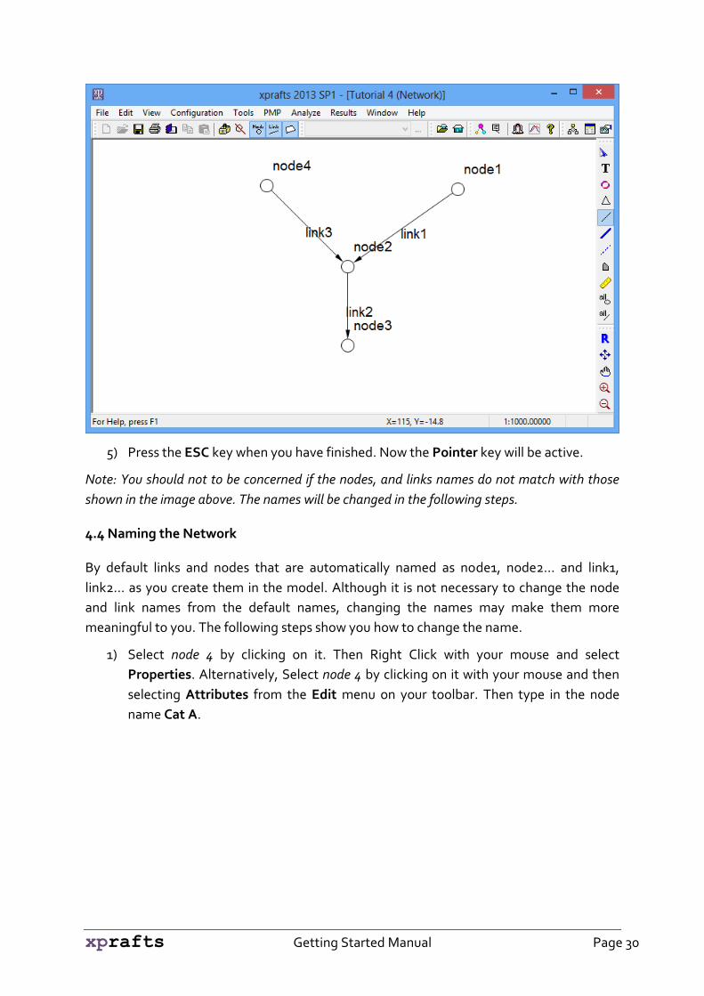
5) Press the ESC key when you have finished. Now the Pointer key will be active.
Note: You should not to be concerned if the nodes, and links names do not match with those
shown in the image above. The names will be changed in the following steps.
4.4 Naming the Network
By default links and nodes that are automatically named as node1, node2… and link1,
link2… as you create them in the model. Although it is not necessary to change the node
and link names from the default names, changing the names may make them more
meaningful to you. The following steps show you how to change the name.
1) Select node 4 by clicking on it. Then Right Click with your mouse and select
Properties. Alternatively, Select node 4 by clicking on it with your mouse and then
selecting Attributes from the Edit menu on your toolbar. Then type in the node
name Cat A.

xprafts Getting Started Manual Page 31
2) Repeat the procedure with other nodes as shown in the Figure below.
Note that he X and Y coordinates displayed depend on the location of the node in the window
and may differ from those shown in this example. Since the layout is schematic the actual
values are unimportant. However, you can change them at this point if you wish.
3) You may also wish to change the display attributes at this stage. You may edit the
attributes by a group edit as well. Select All Nodes or All Links buttons, go to
Edit/Attributes.

xprafts Getting Started Manual Page 32
4.5 Setting the Global Database Information
Global database information contains all of the relevant data that is shared by various
components within the model. It usually pertains to such information as storm types,
infiltration and other losses. There is also the facility to control your table definition.
1) Select Global Data from the Configuration menu. Alternatively click on Global
Database icon .
2) Highlight Temporal Patterns by clicking on it. Then click on the New button.
3) A new field will appear with the name of TP#1. This can be altered to suit your
requirements by either using the backspace key or by selecting Rename. In this
example we will use the name 60min.

xprafts Getting Started Manual Page 33
4) Whilst the name is still selected click Edit and enter the data as follows:

xprafts Getting Started Manual Page 34
Note: Fraction per time interval is the dimensionless pattern which sums up to 1. For
Australian projects, you can specify the temporal pattern zone based on the ARR 1987 and the
program will automatically picks up the pattern. This will be explained further in the following
tutorials.
5) Click OK to continue.
6) To enter the data for a RAFTS storm, select RAFTS Storms from the Global
Databases dialog. Select New and enter the name Design100Yr-60min.
7) Select Edit to open the Storm Data dialog, enter Average Recurrence Interval as
100 years, under the Average Intensity box select Direct and enter 76.3 mm/hr. For
the Temporal Pattern box, select Reference by clicking on the radio button, then
click on the box to open the Select dialog, highlight 60 min from the list and clicking
on Select. Enter Storm Duration as 60 (min).

xprafts Getting Started Manual Page 35
Note: You can allow xprafts to estimate the intensity from the IFD curves depending upon
zones by choosing the option IFD calculation and ARR Standard Zone. You can get the IFD
values from the Australian Bureau of Meteorology website:
http://www.bom.gov.au/water/designRainfalls/ifd-arr87/index.shtml
8) Select OK to continue.
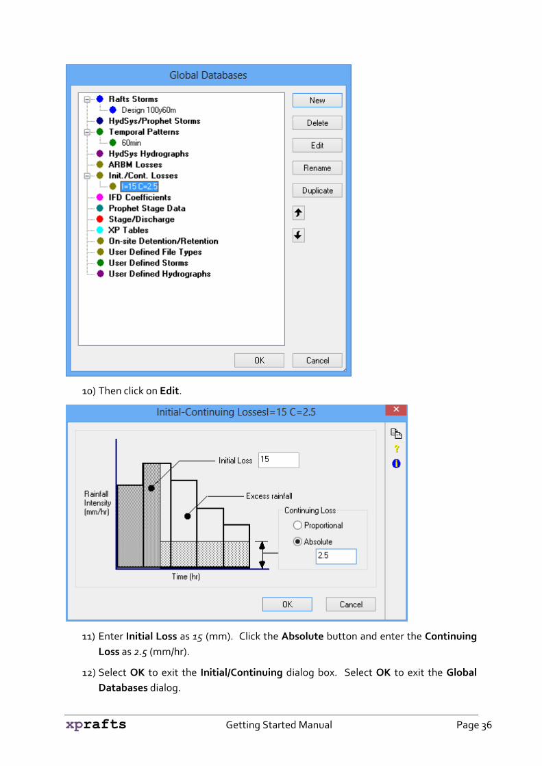
9) To enter the Initial/Continuing Loss data, select Init./Cont. Losses. Then click New
and enter the name IL 15-2.5.
xprafts Getting Started Manual Page 36
10) Then click on Edit.
11) Enter Initial Loss as 15 (mm). Click the Absolute button and enter the Continuing
Loss as 2.5 (mm/hr).
12) Select OK to exit the Initial/Continuing dialog box. Select OK to exit the Global
Databases dialog.
xprafts Getting Started Manual Page 37
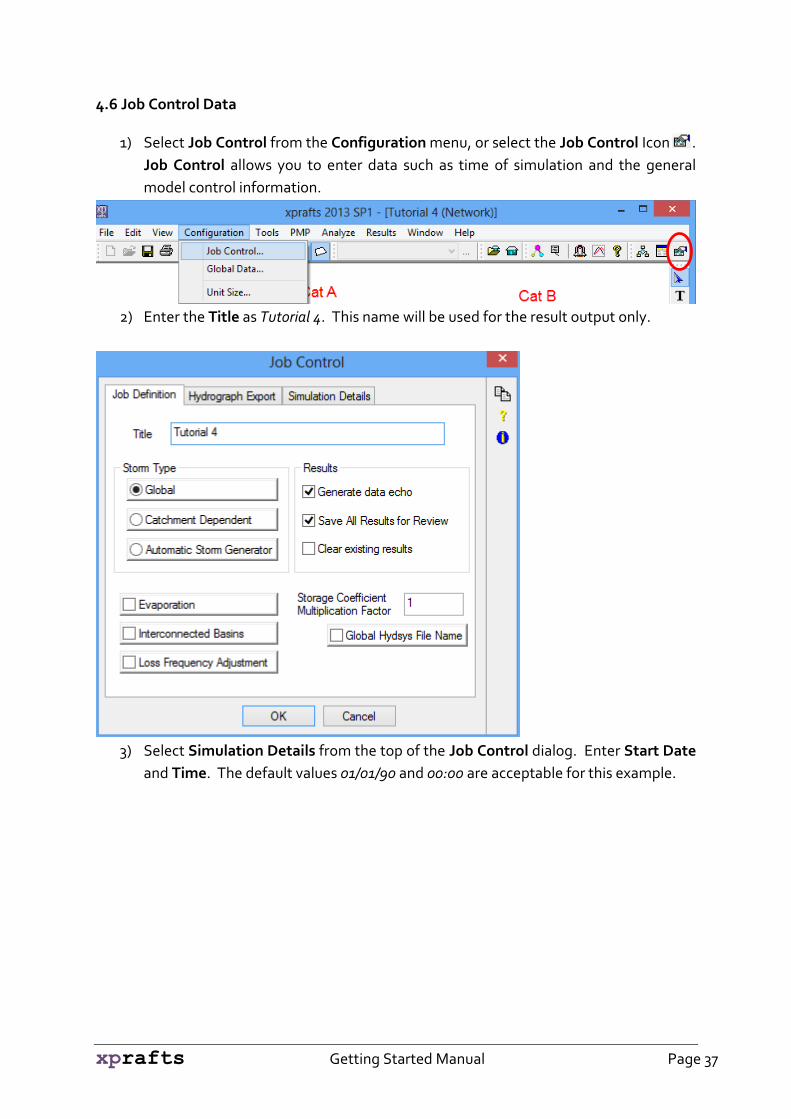
4.6 Job Control Data
1) Select Job Control from the Configuration menu, or select the Job Control Icon .
Job Control allows you to enter data such as time of simulation and the general
model control information.
2) Enter the Title as Tutorial 4. This name will be used for the result output only.
3) Select Simulation Details from the top of the Job Control dialog. Enter Start Date
and Time. The default values 01/01/90 and 00:00 are acceptable for this example.

xprafts Getting Started Manual Page 38
4) Select Job Definition once again. Click on Global to open the Stacked Storms
dialog as shown below.
5) Check the checkbox Use Storm?. Click in the column under Storm Type, a pull
down menu will appear. Select Rafts. Enter Routing Increment as 1 min and
Number of Intervals as 300. Click on Storm Name, select Design 100Yr-60min and
click on Select.
These steps mean that we will simulate the model from 01/01/1990: 00:00 to
01/01/1990: 05:00 (i.e. a duration of 300 minutes).

xprafts Getting Started Manual Page 39
6) Click OK to exit the Stacked Storms dialog. Click OK to exit the Job Control dialog.
4.7 Link Data
1) Select the Link between Cat A and Junction by double clicking on the link3.
2) Enter the LAG time as 2.5 min. Select OK to exit the Lagging Link dialog. Note that
a Lagging Link will lag the upstream hydrograph without any attenuation.
3) With link3 highlighted select Copy Data from the Edit menu.
xprafts Getting Started Manual Page 40
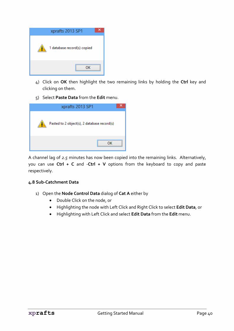
4) Click on OK then highlight the two remaining links by holding the Ctrl key and
clicking on them.
5) Select Paste Data from the Edit menu.
A channel lag of 2.5 minutes has now been copied into the remaining links. Alternatively,
you can use Ctrl + C and -Ctrl + V options from the keyboard to copy and paste
respectively.
4.8 Sub-Catchment Data
1) Open the Node Control Data dialog of Cat A either by
Double Click on the node, or
Highlighting the node with Left Click and Right Click to select Edit Data, or
Highlighting with Left Click and select Edit Data from the Edit menu.
xprafts Getting Started Manual Page 41
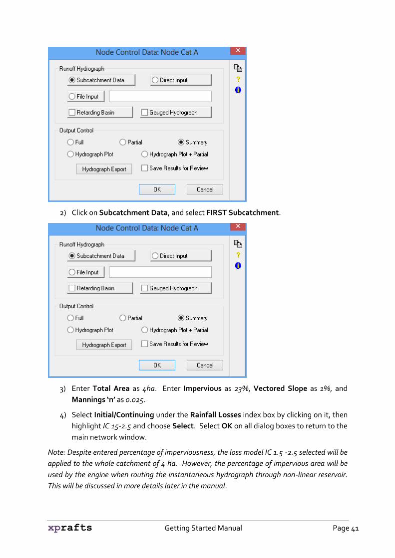
2) Click on Subcatchment Data, and select FIRST Subcatchment.
3) Enter Total Area as 4ha. Enter Impervious as 23%, Vectored Slope as 1%, and
Mannings ‘n’ as 0.025.
4) Select Initial/Continuing under the Rainfall Losses index box by clicking on it, then
highlight IC 15-2.5 and choose Select. Select OK on all dialog boxes to return to the
main network window.
Note: Despite entered percentage of imperviousness, the loss model IC 1.5 -2.5 selected will be
applied to the whole catchment of 4 ha. However, the percentage of impervious area will be
used by the engine when routing the instantaneous hydrograph through non-linear reservoir.
This will be discussed in more details later in the manual.

xprafts Getting Started Manual Page 42
5) Highlight Cat A and select Copy Data from the Edit menu. Now you must select the
nodes where you wish to paste the data. In this example we wish to paste the data
to all the nodes using Select all nodes. You can select multiple nodes by holding
down the Ctrl key whilst you select the interested nodes by Left Clicking on them.
Select Paste Data from the Edit menu. All the catchment and rainfall data, etc.,
that are entered for Cat A, has now been copied into the remaining 3 nodes.
4.9 Saving the File and Solving the Network
1) To save the file, select Save from the File menu or click on the Save Icon from
the toolbar.
2) From the Analyze menu, select Solve or click on the Solve Icon from the
toolbar. This action will solve the network. If any errors are found a Notepad screen
will appear. You will then need to check the data you have entered before solving
again.
4.10 Reviewing Results
1) To review the results for the network highlight the nodes you wish to review and
then select Review Results from the Results menu or click on the Review Results
Icon after highlighting the nodes. The results are shown as follows:

xprafts Getting Started Manual Page 43
You can view maximum of 4 graphs per page by selecting the pull down menu from the top
of the page. Variables can also be viewed separately or grouped in a single graph. You can
zoom in, change the font size, the style of graphs or show legends, ect., by Left Clicking and
choose from the drop down menu.
2) When you have finished reviewing the results click on the lower cross in the top right
hand corner of the Review Results window. This will return you to the network
view.
4.11 Exiting Program
To exit the program, select Exit from the File menu or click on the cross on the right hand
corner of the page.

xprafts Getting Started Manual Page 44
Tutorial 5: Linking To External Databases
5.1 Introduction
This tutorial describes the integration of xprafts and the commercial programs used
ODBC compliant databases such as Microsoft Access, Microsoft Excel, ESRI Arc View, and
MapInfo. The process allows that data which already exist in Asset Management Systems
and Geographic Information Systems (GIS) can be directly linked to the software for use in
the development of the simulation model. While this process is an extremely efficient
method of transferring data between the GIS and model, it may be further automated by
the creation of scripts within the respective GIS packages to produce seamless integration
of the software and GIS.
5.2 Setting up the Model
First we will setup the blank model and then link with the external database.
1) Click on Blank Job in the File\New Menu. Alternatively use Ctrl + N from keyboard.
2) Type in the model name as Tutorial 5 and click on Save.
Now you have a blank model to link with the external database.
5.3 Linking with External Database
1) From the File menu, select the option Import External Databases.

xprafts Getting Started Manual Page 45
2) Now click on the Select File tab
3) Now browse for the file Model_Data.mdb in Tutorial 5 folder, then Left Click on the
file and Open.
You can see that there is another file, Model_Data.xls, which contains the same data
as Model_Data.mdb . You may select this excel file instead of the *.mdb file.
xprafts Getting Started Manual Page 46
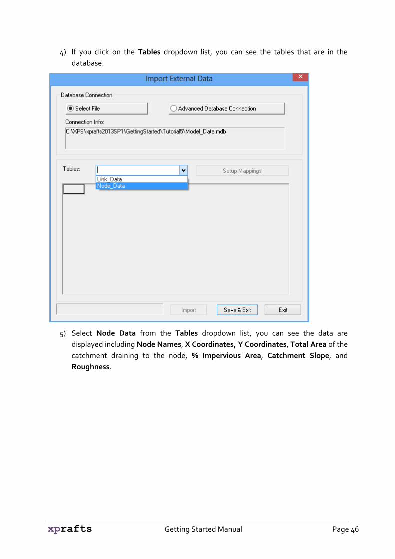
4) If you click on the Tables dropdown list, you can see the tables that are in the
database.
5) Select Node Data from the Tables dropdown list, you can see the data are
displayed including Node Names, X Coordinates, Y Coordinates, Total Area of the
catchment draining to the node, % Impervious Area, Catchment Slope, and
Roughness.

xprafts Getting Started Manual Page 47
6) Click on Setup Mappings in the Import External Data dialog to open Variable
Mappings. We will map the variables in the database against the variables in the
xprafts database. For example, “Catchment Roughness” in the external
database will be mapped against “Catchment Manning’s n” in the xprafts
database.
7) Select Object Type & Mandatory Data as Node first. Now, we will map the
Mandatory Data which are the essential data required to create node entities. The
Mandatory Data are Node Names and Positions. Use the dropdown button and
select “Node Name” for “Node”, “X Co-ordinate” for “X Pos”, and “Y Co-ordinate”
for “Y Pos”.

xprafts Getting Started Manual Page 48
8) From Fields in the Variable Mappings dialog, Left Click and highlight Total Area
(Ha) then click on Insert Mapping.
9) Select Total Area under Subcatchment in the Node Variables dialog and click on
OK. Now you can see that Total Area (Ha) in the external Database is mapped
against the Total Area in Subcatchment in xprafts.

xprafts Getting Started Manual Page 49
Note the red question mark (?) in Fields (in the Variable Mappings dialog) has been
changed to a green tick mark.
Repeat the steps to map all variables as shown in the table below.
Node Name Node
X Pos X Co-ordinate
Y Pos Y Co-ordinate
Total Area (Ha) Total Area
Impervious % Percentage Impervious
Catchment Roughness Catchment Mannings ‘n’
Catchment Slope (%) Catchment slope
10) Click on OK after completion of mapping. Click on Import in the next dialog.
You can see that 11 nodes have been imported from the external database. Click on
OK.
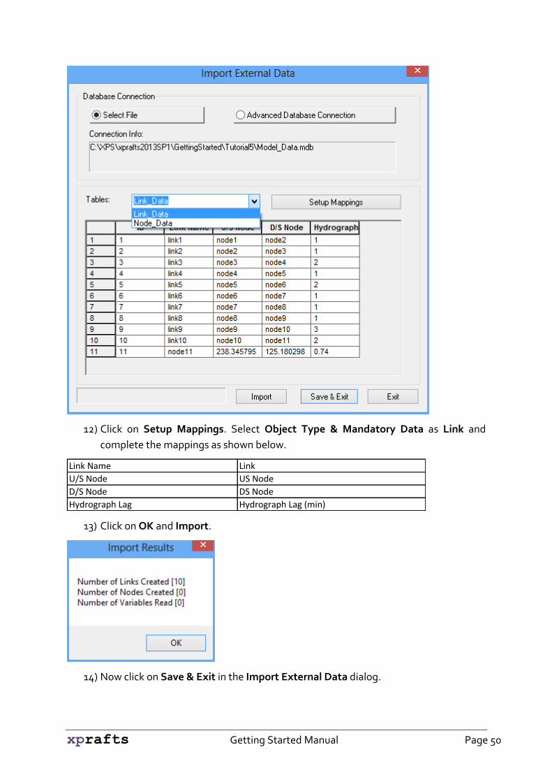
11) Similarly we will prepare the mapping for each of the link variables. Select the Link
Data table as shown below:
xprafts Getting Started Manual Page 50
12) Click on Setup Mappings. Select Object Type & Mandatory Data as Link and
complete the mappings as shown below.
Link Name Link
U/S Node US Node
D/S Node DS Node
Hydrograph Lag Hydrograph Lag (min)
13) Click on OK and Import.
14) Now click on Save & Exit in the Import External Data dialog.
xprafts Getting Started Manual Page 51
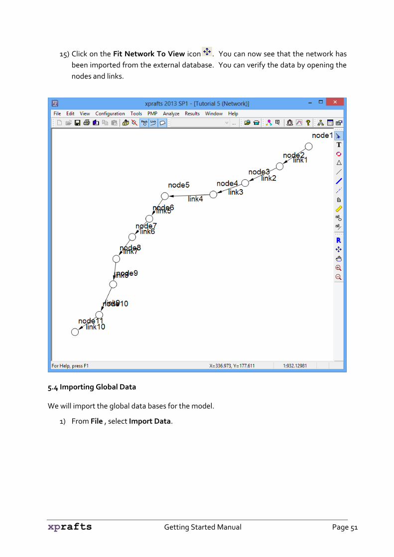
15) Click on the Fit Network To View icon . You can now see that the network has
been imported from the external database. You can verify the data by opening the
nodes and links.
5.4 Importing Global Data
We will import the global data bases for the model.
1) From File , select Import Data.

xprafts Getting Started Manual Page 52
2) Select GlobalData.xpx and click on Open.
3) Double Click on any node and select Subcatchment Data, then select FIRST
Subcatchment and click on Initial/Continuing Loss. Highlight rural and click on
Select to return to the Subcatchment Data dialog.
Note: these databases are imported from *.xpx file.

xprafts Getting Started Manual Page 53
4) Click on Copy Icon in the Subcatchment Data dialog, then click on the
Initial/Continuing box with rural selected, a pop-up window will tell you what has
been copied. Click on OK to return the network window.
5) In the main network window, highlight all nodes using the Select all nodes Tool, go
to Edit on the main menu, select Paste Data and xprafts notifies you how
many objects and database records have been pasted. Click on OK.
xprafts Getting Started Manual Page 54
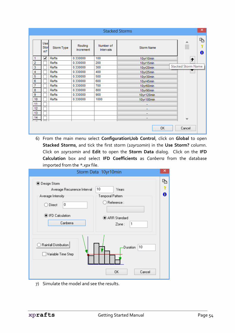
6) From the main menu select Configuration\Job Control, click on Global to open
Stacked Storms, and tick the first storm (10yr10min) in the Use Storm? column.
Click on 10yr10min and Edit to open the Storm Data dialog. Click on the IFD
Calculation box and select IFD Coefficients as Canberra from the database
imported from the *.xpx file.
7) Simulate the model and see the results.
xprafts Getting Started Manual Page 55
Tutorial 6: Subdivision - Pre Development
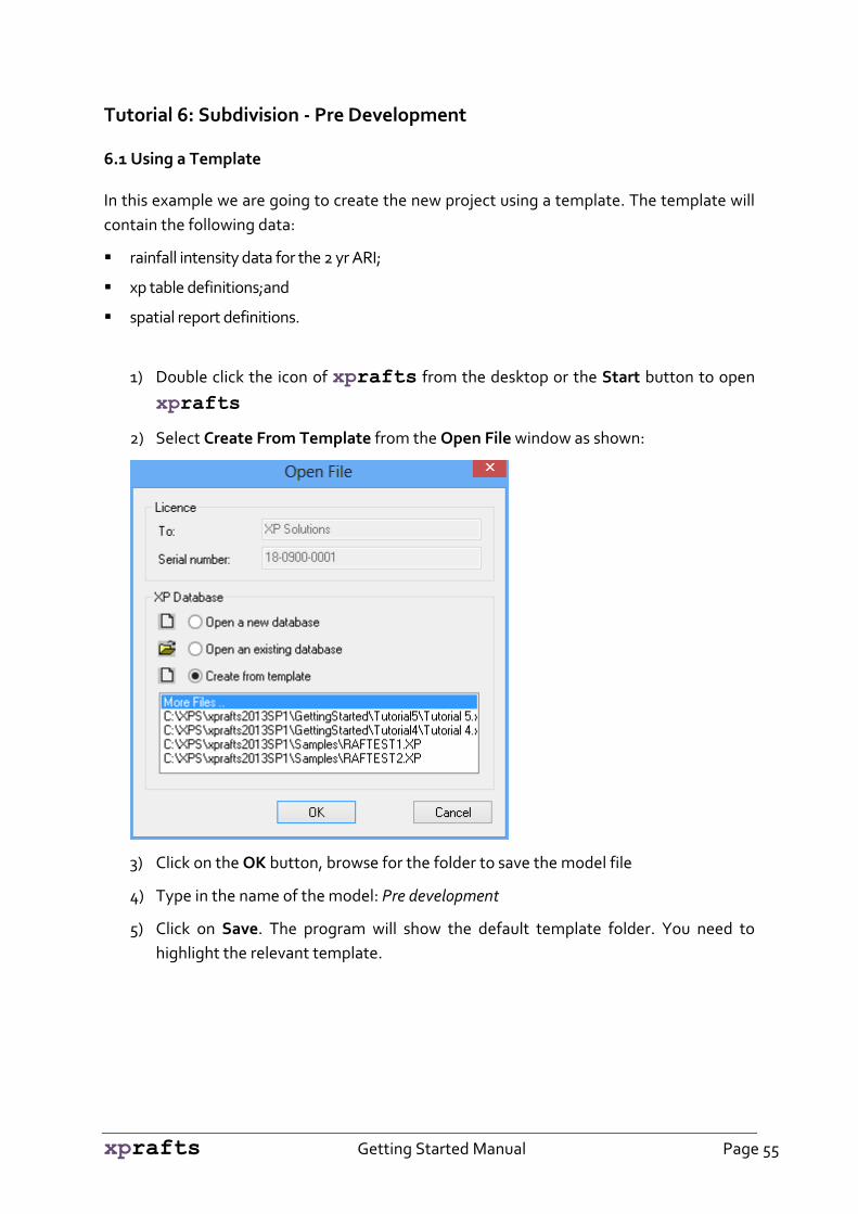
6.1 Using a Template
In this example we are going to create the new project using a template. The template will
contain the following data:
rainfall intensity data for the 2 yr ARI;
xp table definitions;and
spatial report definitions.
1) Double click the icon of xprafts from the desktop or the Start button to open
xprafts
2) Select Create From Template from the Open File window as shown:
3) Click on the OK button, browse for the folder to save the model file
4) Type in the name of the model: Pre development
5) Click on Save. The program will show the default template folder. You need to
highlight the relevant template.

xprafts Getting Started Manual Page 56
6) Click on Cairns.xpt for this model
7) Click on Open (If you save your template files in any other folder, then you need to
browse for it and open).
The window will appear and we will be using the tool strips on the top and right side.
6.2 Adding a Background Image and Zoom Tool
We will now add an optional background image as a reference for our sub division.
1) Click on New Background Image Icon from the top tool strip and the Add
Background Image dialog will appear.
2) Click on the ellipsis (…) to browse for the folder
C:\XPS\xprafts2013SP1\GettingStarted\Tutorial5 select the file Development.dwg
and then click on Open.

xprafts Getting Started Manual Page 57
You can add images with different extensions. The available file formats are AutoCAD
*.dwg, and *.dxf formats, ESRI *.shp files, and image files such as *.bmp, *.tiff, *.jpg, etc.
In this tutorial we will use an AutoCAD file with the extension of *.dwg. The entire extent
of the drawing will be displayed so we will have to zoom into the project area.
3) Click on the Zoom In Icon from the right tool strip.

xprafts Getting Started Manual Page 58
4) Drag a rectangle around the project area to zoom in. Alternatively, you can use the
scroll button of the mouse to zoom in and zoom out on the background image. The
right mouse button can be used always to pan apart from the Pan Tool).
6.3 Creating Nodes
Now we are going to create nodes to represent the project area before development.
1) Select the Node Tool , you will see that the cursor has changed to .
2) Click on the locations where you want to create nodes. In this tutorial, we will create
4 nodes as shown in the image below. Press ESC to stop creating nodes, you will see
that cursor has changed to the Pointer Tool .

xprafts Getting Started Manual Page 59
6.4 Creating Links
Now we will create links by connecting the nodes.
1) From the right tool strip, select the Link Tool .The cursor will change to .
2) Left Click on node 1 and continue Left Clicking on all the nodes, when you reach
node 4, press ESC button. Each time you reach to a node the cursor will change to a
red cross , i.e. you snap the node.

xprafts Getting Started Manual Page 60
3) You can now see that links have been created as shown in the image below. Note
that these links are lagging links, where hydrographs are just delayed without
attenuation.
6.5 Creating Catchments
Sub-catchments can be created using the Create Subcatchment tool .
1) Select this tool from the right tool strip and you will see the change in the cursor
2) Digitize the catchment by Left Clicking of the mouse, once you finish, Double Click
to end.
3) Now, make sure that the Lock Catchment Icon is switched off .
4) Left click on the catchment polygon, hover the cursor over the catchment polygon
and you will see the Pointer Tool is changed when the cursor reaches the
catchment centroid.
5) Keep the left button of the mouse pressed and move towards node1, once it reaches
the node’s location the cursor will change , release the mouse button then from
the pop-up menu choose Drain Catchment As and connect catchment as
Subcatchment 1.

xprafts Getting Started Manual Page 61
6)
7) 8) Now, go to the Tools menu and select Calculate Node, and Calculate Area.

xprafts Getting Started Manual Page 62
9) You can see that the catchment area is computed. Click on OK in the next dialogue.
10) Alternatively, we can measure the catchment area using the Ruler Tool . Click the
on the Ruler Tool from the right tool strip. Draw the catchment boundary. Once the
cursor reaches the starting point, the shape will be changed to cross. While moving
the cursor, you will see that the Ruler Tool measures the Total Distance traversed
and as you reach the starting point, the Total Area will be shown.
11) Double click on the node1 to open the Node Control Data dialog.
12) Click on Subcatchment Data to open the Catchment Data dialog.

xprafts Getting Started Manual Page 63
13) Click on FIRST Subcatchment. You will not use the SECOND Subcatchment for
this tutorial.
14) You can see that the calculated area (Total Area) is assigned to the catchment.

xprafts Getting Started Manual Page 64
15) Type in the subcatchment data. The pre developed area has a Vectored Slope of
0.5% grade and a Manning’s n value of 0.025, and Impervious of 0%.
Note: The percentage of Impervious is an indicator for the urbanization of the lot. This
value does not affect the volume of rainfall losses. The loss model specified for the
catchment will be applied for the whole area, 0.562 ha, regardless of the impervious
percentage entered. However, it will be used when routing the instantaneous hydrographs
through the non-linear storage reservoirs. Please refer to Equation 8 in the Chapter 14 –
RAFTS theory, under coefficients B and n section in the help file. The percentage of
Impervious will be used as “U” in Equation 8. If you wish to model some part of the
catchment with another loss model (says impervious area losses), create a second
catchment with the new loss model.
6.6 Initial/Continuing Rainfall Loss Model
To model the rainfall losses we will use the Initial/continuing loss model.
1) Click on Initial/Continuing Rainfall Loss in the dialog above Subcatchment Data,
and select 20l 5C in the Seclect dialog box. If you want to review the data, click on
Edit

xprafts Getting Started Manual Page 65
2) The loss models included in the template are shown in the Global Databases dialog.
Click Edit to review the data for training purposes.
Note that the first 20 mm of rainfall is lost, then 5mm/hr for the remaining of the
rainfall event. Click OK to finish entering the data and click on Select in the next
dialogue.
3) With 20I 5C highlighted in the Select dialog click on the Copy Icon on the top-
right of the Subcatchment Data dialog . This will copy the data containing in 20I 5C.

xprafts Getting Started Manual Page 66
From the dialog you can see that the loss model has been copied, click on OK on all
the dialogues until you reach the main window.
4) Click on Select all nodes Tool , and press Ctrl + V on the keyboard to paste the
copied database to all the nodes.
Note that a loss model should be specified to all the nodes to run the engine.
6.7 Reviewing Rainfall Data
Before we calculate the hydrographs for this project we will review the rainfall data that
was included in the template.
1) Click on the Job Control Icon from the top tool strip or click on Configuration from
the menu bar and select Job Control.

xprafts Getting Started Manual Page 67
2) Click on the Global radio button under Storm Type. The global storms shown in
Stacked Storms are the temporal patterns from ARR volume 2.
3) Routing Increment of 1 minute is selected and Number of Intervals of 4380 min
selected is long enough for the longest rainfall event. Note that Number of Intervals
should be in an ascending order.
xprafts Getting Started Manual Page 68
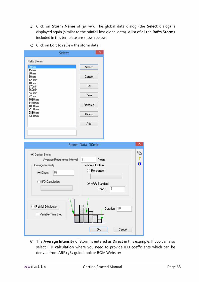
4) Click on Storm Name of 30 min. The global data dialog (the Select dialog) is
displayed again (similar to the rainfall loss global data). A list of all the Rafts Storms
included in this template are shown below.
5) Click on Edit to review the storm data.
6) The Average Intensity of storm is entered as Direct in this example. If you can also
select IFD calculation where you need to provide IFD coefficients which can be
derived from ARR1987 guidebook or BOM Website:
xprafts Getting Started Manual Page 69
http://www.bom.gov.au/water/designRainfalls/ifd-arr87/index.shtml
Average Recurrence Interval (ARI) under Design Storm, ARR Standard Zone
under Temporal Pattern and Duration are entered using the temporal pattern from
ARR volume 2 (these data are stored in the engine). The Average Intensity of
rainfall entered is then applied to this temporal pattern.
7) Click OK, then Select and then OK on each dialog to close them all.
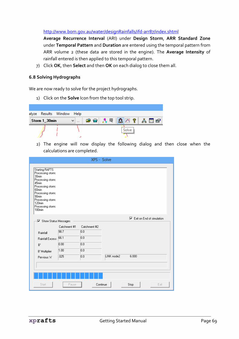
6.8 Solving Hydrographs
We are now ready to solve for the project hydrographs.
1) Click on the Solve Icon from the top tool strip.
2) The engine will now display the following dialog and then close when the
calculations are completed.
xprafts Getting Started Manual Page 70
3) Results are written to a file with the extension of *.out and has the same name as
your project’s name. The result data can be viewed either by displaying in the
interface of the software or reading from the text interface.
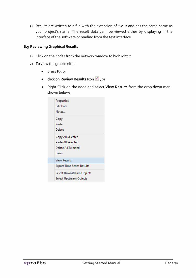
6.9 Reviewing Graphical Results
1) Click on the node1 from the network window to highlight it
2) To view the graphs either
press F7, or
click on Review Results Icon , or
Right Click on the node and select View Results from the drop down menu
shown below:

xprafts Getting Started Manual Page 71
3) Results for All Storms will be displayed with the peak runoffs. You can see that 540
min storm gives the peak runoff value of 0.097 cms for the predevelopment site. To
view other storms select them from the dropdown list for storms.
Peak Runoff Value

xprafts Getting Started Manual Page 72
4) Zoom in by dragging a rectangle around the desired area. The example below shows
rainfall and excess rainfall.
5) Right Click in the graph area and select Undo Zoom from the drop down menu to
zoom out to the full extent.
Initial Loss (20mm)
Continuing Loss (5mm/hr)
xprafts Getting Started Manual Page 73
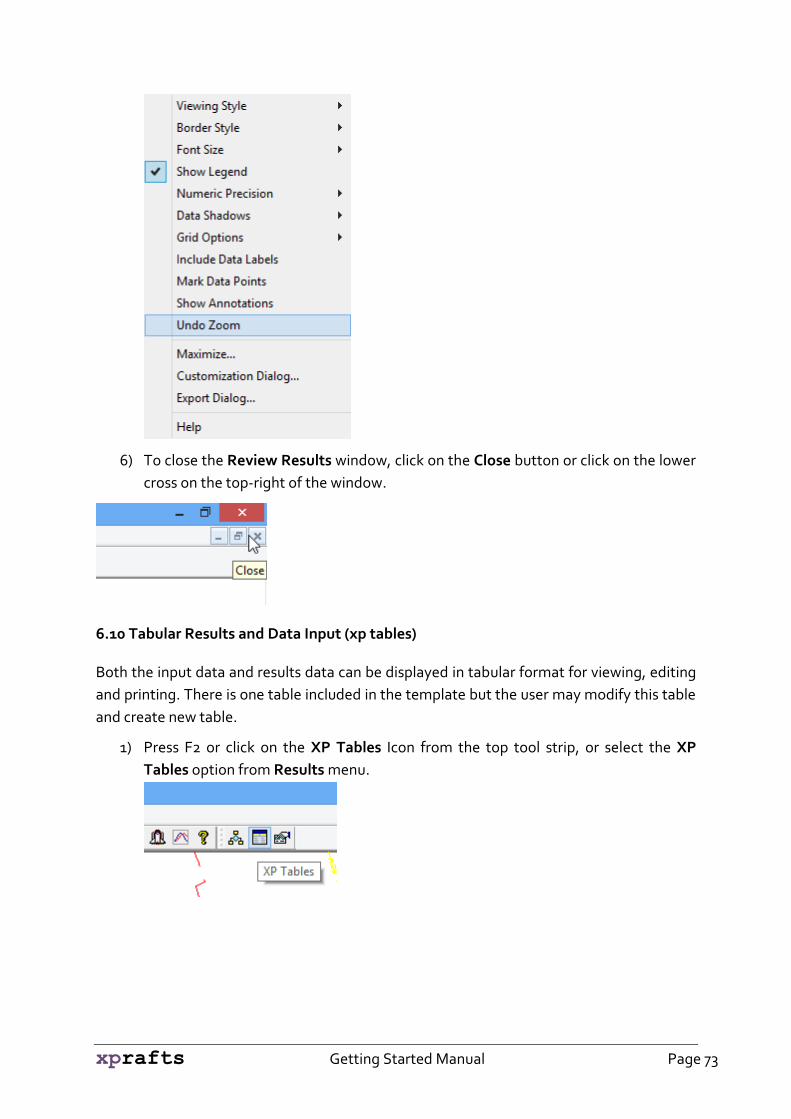
6) To close the Review Results window, click on the Close button or click on the lower
cross on the top-right of the window.
6.10 Tabular Results and Data Input (xp tables)
Both the input data and results data can be displayed in tabular format for viewing, editing
and printing. There is one table included in the template but the user may modify this table
and create new table.
1) Press F2 or click on the XP Tables Icon from the top tool strip, or select the XP
Tables option from Results menu.

xprafts Getting Started Manual Page 74
2) The table name that is already defined and imported from the template will be
displayed. Click on View.
3) By default, Critical Storm is displayed. You can select the storm and other data and
results to view.

xprafts Getting Started Manual Page 75
Tutorial 7: Subdivision - Post Development
This tutorial begins by creating the job with the Cairns template used in the previous
example but it will be saved as ‘post development’.
The layout of the post development plan is shown below.
Individual lots
Post
developments –
impervious areas
Proposed detention
basin site
7.1 Entering Nodes and Links for the Post Developed Site
1) Enter nodes and links in the locations shown in the layout as in Tutorial 5 (section 5.3
and 5.4). To create links that have polyline shapes hold the Ctrl key and digitize it.
2) Right Click on each node and link and select Attributes. You will be able to change
the names and other display attributes here. Alternatively a group of attributes can
be edited by selecting all nodes and links using Select all nodes and Select all links
then select Attributes from the Edit menu.

xprafts Getting Started Manual Page 76
7.2 Splitting Catchments into Pervious and Impervious subcatchments.
In this section we will import an *.xpx file which contains the development lots polygon.
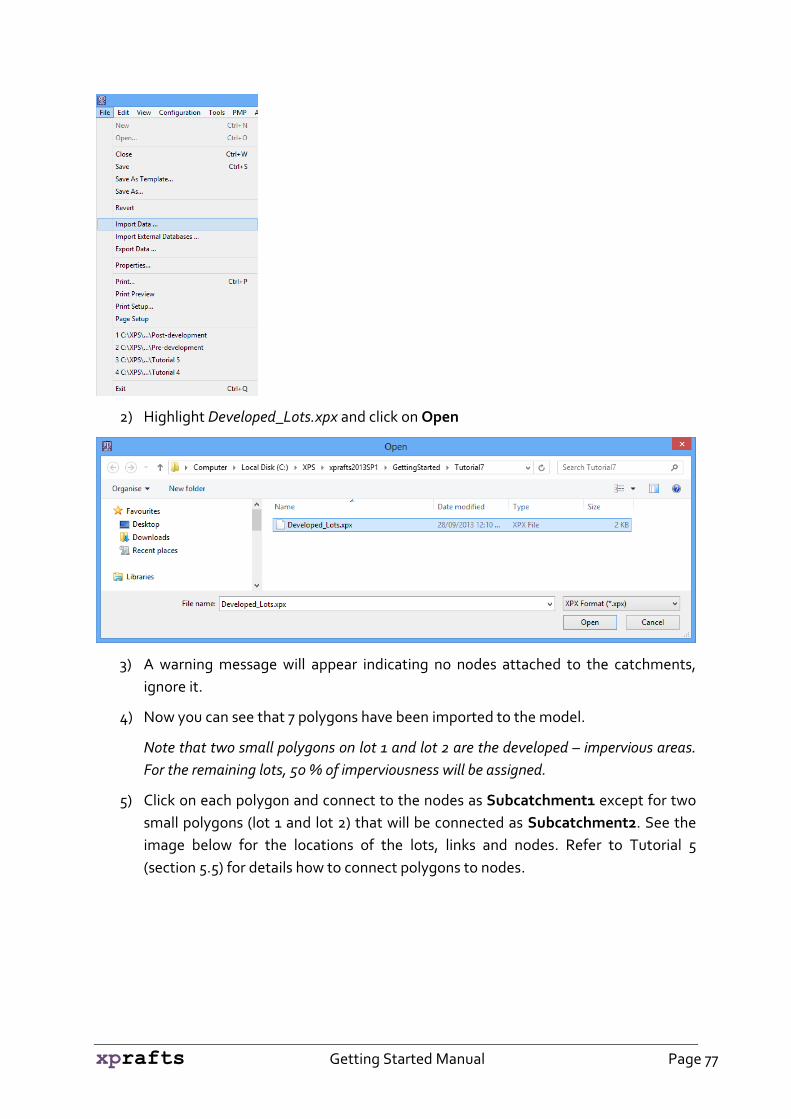
1) Go to the File menu and select Import Data
xprafts Getting Started Manual Page 77
2) Highlight Developed_Lots.xpx and click on Open
3) A warning message will appear indicating no nodes attached to the catchments,
ignore it.
4) Now you can see that 7 polygons have been imported to the model.
Note that two small polygons on lot 1 and lot 2 are the developed – impervious areas.
For the remaining lots, 50 % of imperviousness will be assigned.
5) Click on each polygon and connect to the nodes as Subcatchment1 except for two
small polygons (lot 1 and lot 2) that will be connected as Subcatchment2. See the
image below for the locations of the lots, links and nodes. Refer to Tutorial 5
(section 5.5) for details how to connect polygons to nodes.

xprafts Getting Started Manual Page 78
6) Now go to the Tools menu, select Calculate Node, and then choose Catchment
Area (see Tutorial 5 (section 5.5)). The catchment areas will be calculated as shown
below.
To change the rainfall losses for the impervious areas, we will create another loss model
called ‘impervious’. This loss model will be applied to the SECOND catchment area. The

xprafts Getting Started Manual Page 79
Manning’s n value will be changed for the impervious area to represent the roughness of
concrete surfaces.
7) We will create the new rainfall loss model for the impervious-developed areas via
Configuration on the menu bar, select Global data, then select Init/Cont Losses
and then click on New.
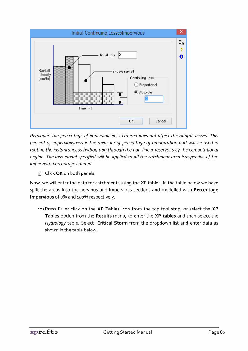
8) Type in the name ‘impervious’ and click on Edit. Enter values of Initial Loss and
Continuing Loss as shown in the dialog below.
Note that we use a small initial loss (2 mm) and then no continuing loss (0 mm/h) for
the impervious area.
xprafts Getting Started Manual Page 80
Reminder: the percentage of imperviousness entered does not affect the rainfall losses. This
percent of imperviousness is the measure of percentage of urbanization and will be used in
routing the instantaneous hydrograph through the non-linear reservoirs by the computational
engine. The loss model specified will be applied to all the catchment area irrespective of the
impervious percentage entered.
9) Click OK on both panels.
Now, we will enter the data for catchments using the XP tables. In the table below we have
split the areas into the pervious and impervious sections and modelled with Percentage
Impervious of 0% and 100% respectively.
10) Press F2 or click on the XP Tables Icon from the top tool strip, or select the XP
Tables option from the Results menu, to enter the XP tables and then select the
Hydrology table. Select Critical Storm from the dropdown list and enter data as
shown in the table below.
xprafts Getting Started Manual Page 81
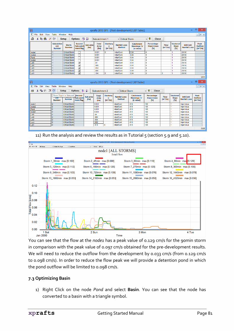
11) Run the analysis and review the results as in Tutorial 5 (section 5.9 and 5.10).
You can see that the flow at the node1 has a peak value of 0.129 cm/s for the 90min storm
in comparison with the peak value of 0.097 cm/s obtained for the pre-development results.
We will need to reduce the outflow from the development by 0.033 cm/s (from 0.129 cm/s
to 0.098 cm/s). In order to reduce the flow peak we will provide a detention pond in which
the pond outflow will be limited to 0.098 cm/s.
7.3 Optimizing Basin
1) Right Click on the node Pond and select Basin. You can see that the node has
converted to a basin with a triangle symbol.

xprafts Getting Started Manual Page 82
2) Double Click on the basin node to open Node Control Data and then click on
Retarding Basin.
To start the design we enter the level for the basin bed as 12.7 m. Next we must enter
the compulsory data for Retarding Basin (the boxes with no tick boxes).
3) Click on Storage in the Retarding Basin dialog and enter the data as below.

xprafts Getting Started Manual Page 83
Note: If the first level of the basin is 0.0m, it means that the level data is considered
relative to the basin invert level entered above. In this case we are using the actual
levels.
xprafts Getting Started Manual Page 84
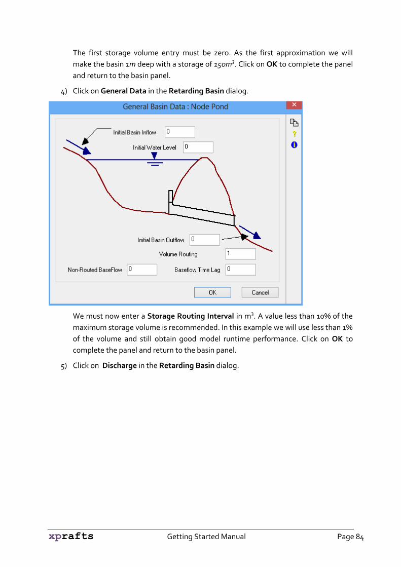
The first storage volume entry must be zero. As the first approximation we will
make the basin 1m deep with a storage of 150m3. Click on OK to complete the panel
and return to the basin panel.
4) Click on General Data in the Retarding Basin dialog.
We must now enter a Storage Routing Interval in m3. A value less than 10% of the
maximum storage volume is recommended. In this example we will use less than 1%
of the volume and still obtain good model runtime performance. Click on OK to
complete the panel and return to the basin panel.
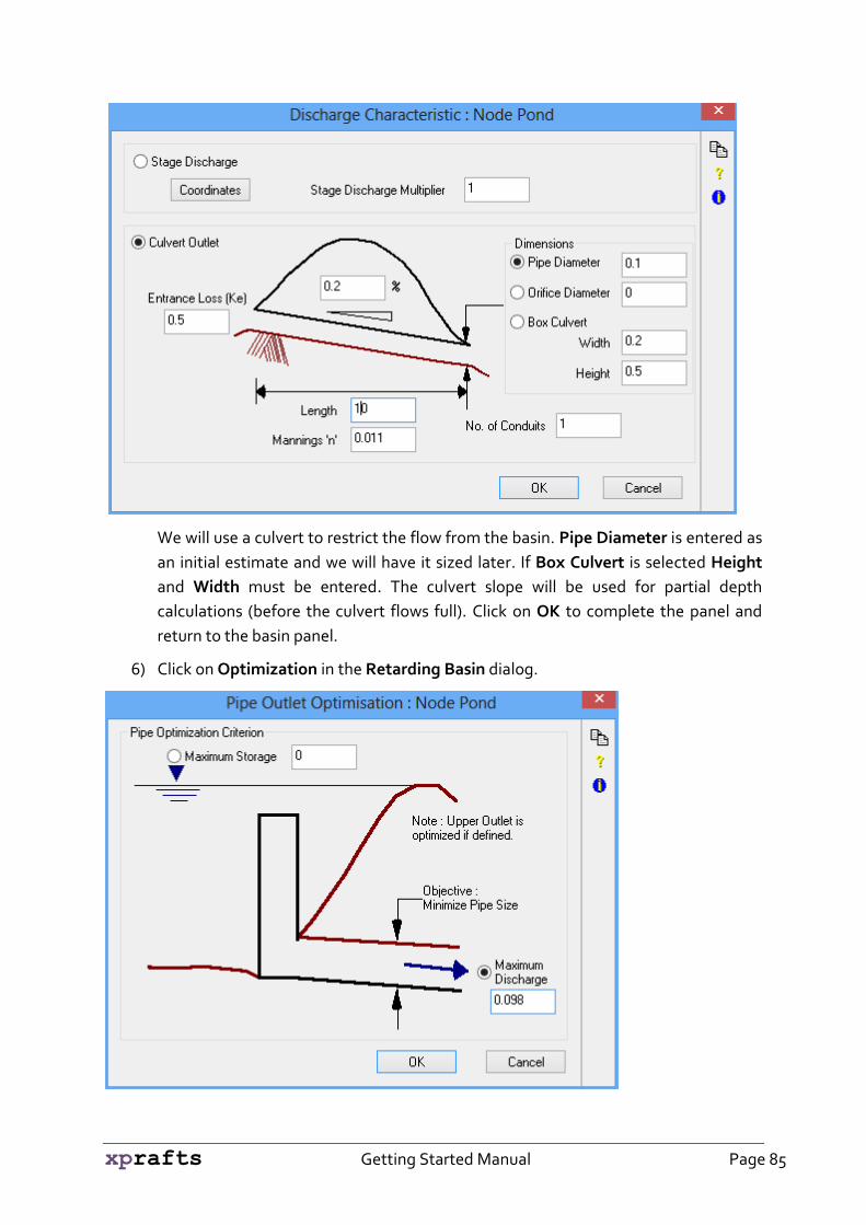
5) Click on Discharge in the Retarding Basin dialog.
xprafts Getting Started Manual Page 85
We will use a culvert to restrict the flow from the basin. Pipe Diameter is entered as
an initial estimate and we will have it sized later. If Box Culvert is selected Height
and Width must be entered. The culvert slope will be used for partial depth
calculations (before the culvert flows full). Click on OK to complete the panel and
return to the basin panel.
6) Click on Optimization in the Retarding Basin dialog.

xprafts Getting Started Manual Page 86
Here we will specify the maximum desired discharge and will size the outlet. The
resulting basin depth and storage can then be checked to see if they are acceptable.
Since we will be running several storms, it is unlikely that the same pipe diameter
will be selected for each storm.
7) Run the model using Solve
8) To review the culverts sizes and the output file, click on Results from the menu bar,
then select Browse File… and select the result file *.out. Alternatively you can press
F6 to browse for the result file.
9) In this case a pipe with diameter of 0.275 m was suggested. The depth in the basin
reached 13.266 m for this storm. If this is considered too deep, then the basin area
will have to be increased.
10) Return to Node4 to see if the discharge has been reduced to the pre-development
level.

xprafts Getting Started Manual Page 87
You can see that the maximum discharge now is equal to the pre-development case
(0.096 cms). Once you have finalized your outlet pipe size return to the basin panel,
untick Optimization and click Discharge to enter the final pipe size. Remember to
enter the maximum height observed in your basin. This can be found by reviewing
results for the basin and selecting basin stage.
11) Once the lower outlet is designed for the minor event we can design for the major
event. This requires to change the rainfall intensities and return periods in the
global storms. Once you have done this, return to the Retarding Basin dialog and
select Normal Spillway.
3 Enter a trial Width and run the model to check the final basin Height and
Discharge for the 100 year ARI event. You may have to alter the spillway
width to change these results. The discharge coefficient may change
depending on your weir crest shape.

xprafts Getting Started Manual Page 88

xprafts Getting Started Manual Page 89
Tutorial 8: River Example
8.1 River Example Introduction
Results from xprafts provide flow hydrographs at any point along the river over the
simulation period. In this tutorial we will use about 5-month time series of data. The
example can also be used in flood forecasting to predict flows in future times. xprafts
can also be directly linked to the hydraulic layer of xpswmm to provide accurate water
levels along each reach. The simulation can be dynamically replayed on screen.
Browse to the folder C:\XPS\xprafts2013\GettingStarted\Tutorial7 and open the file River
Example.xp
8.2 Link and Node Data
1) From the Results menu select XP Tables.
Note that you can use F2 key as a shortcut to access the XP-Tables.
2) Select Link in XP Table Options and click on View.
The Table shows all information about links in the job, including Link type – Routing or
Lagging, Channel routing X, Channel routing K, Type of channel data entry direct or
calculated.
xprafts Getting Started Manual Page 90
3) Click on the cross in the right corner of the window to close the dialog when you
have finished.
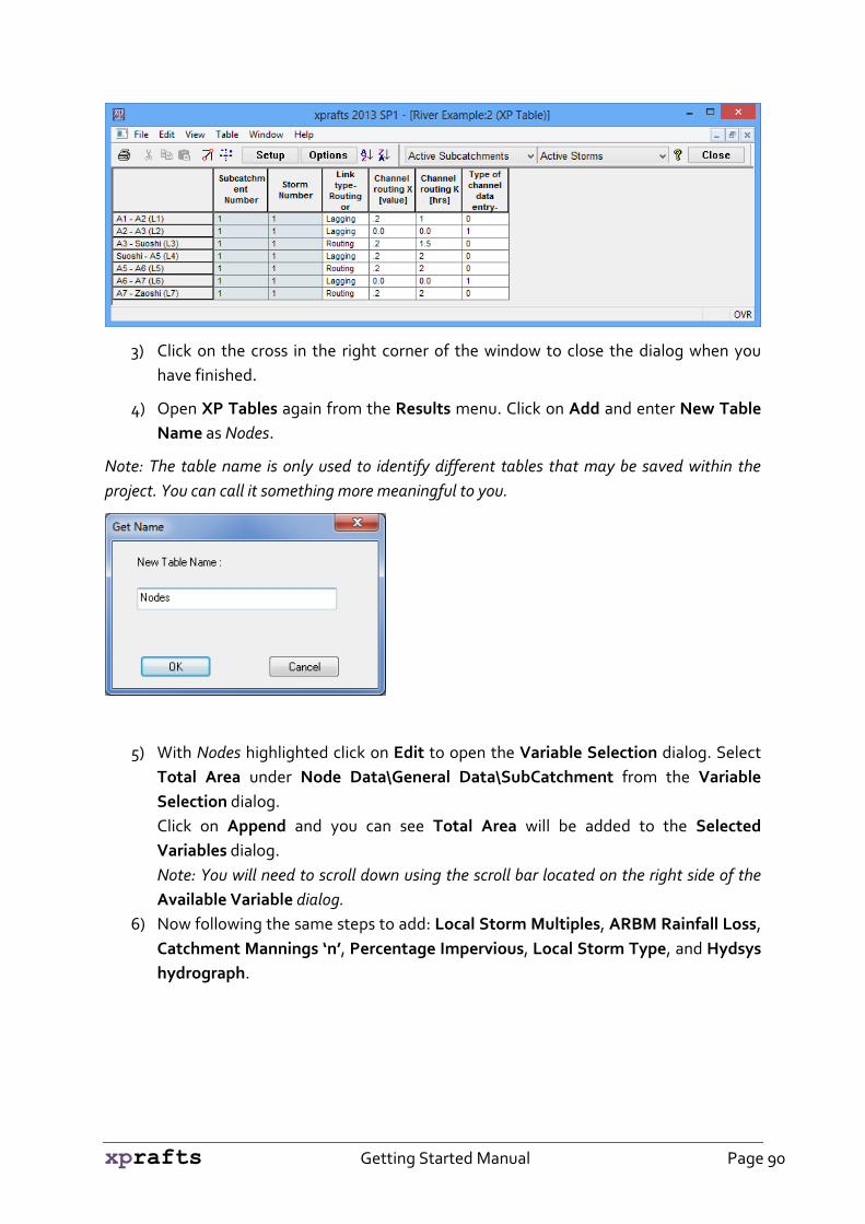
4) Open XP Tables again from the Results menu. Click on Add and enter New Table
Name as Nodes.
Note: The table name is only used to identify different tables that may be saved within the
project. You can call it something more meaningful to you.
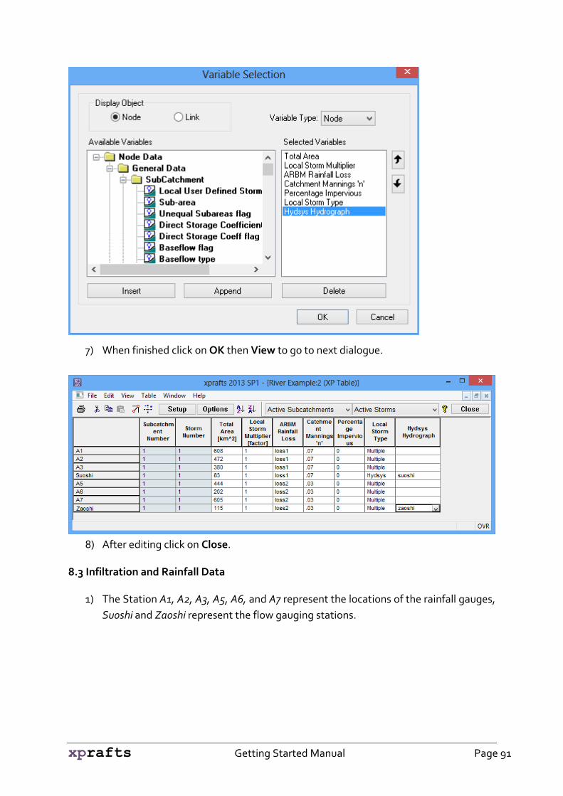
5) With Nodes highlighted click on Edit to open the Variable Selection dialog. Select
Total Area under Node Data\General Data\SubCatchment from the Variable
Selection dialog.
Click on Append and you can see Total Area will be added to the Selected
Variables dialog.
Note: You will need to scroll down using the scroll bar located on the right side of the
Available Variable dialog.
6) Now following the same steps to add: Local Storm Multiples, ARBM Rainfall Loss,
Catchment Mannings ‘n’, Percentage Impervious, Local Storm Type, and Hydsys
hydrograph.
xprafts Getting Started Manual Page 91
7) When finished click on OK then View to go to next dialogue.
8) After editing click on Close.
8.3 Infiltration and Rainfall Data
1) The Station A1, A2, A3, A5, A6, and A7 represent the locations of the rainfall gauges,
Suoshi and Zaoshi represent the flow gauging stations.

xprafts Getting Started Manual Page 92
2) Double click the node A1 in the main network window to open the Node Control
Data dialog, click on Subcatchment Data, select FIRST Subcatchment, then tick
the ARBM radio button and click on the ARBM box to select rainfall losses called
loss 1.
3) With loss 1 highlighted in the Select dialog click on Edit.

xprafts Getting Started Manual Page 93
4) Click on the Infiltration, etc. tab. Here you can enter the data for Upper Soil, Lower
Soil Drainage Factor and Groundwater Recession Factors.

xprafts Getting Started Manual Page 94
5) Click on OK to exit the dialog, then click on the cross in the right corner to close the
Select box, and return to Subcathment Data.
6) Click on Local Storm. Select Multiple Hydsys Storms as shown below. If you wish
to see the data, click on the Storm Name column and select HydSys/Prophet
Storms, then select Edit to open the Hydsys Storm dialog. Click on OK or the cross
to exit the dialogs.

xprafts Getting Started Manual Page 95
7) Click OK to close all dialogs.
8.4 Weighted Rainfall Data to Individual Sub-Catchments
1) Select Global Data from the Configuration menu.

xprafts Getting Started Manual Page 96
2) Highlight Nishi under HydSys/Prophet Storms then select Edit. Alternatively you
can double click on Nishi to open the Hydsys Storm dialog.
3) Click on Edit. The program will then display the Date, Time and Rainfall
information. Click on Graph to view the Hydsys graph for the station.

xprafts Getting Started Manual Page 97
4) Repeat the steps for the Station Nanping.
8.5 Gauged Flow or Stage Data
1) Open the Node Control Data dialog for the Station Suoshi by double clicking on it in
the main window.
2) Double Click on Gauged Hydrograph, select the Hydsys Hydrograph radio button,
then click on the Hydsys Hydrograph box. In this example it is labeled as Suoshi.

xprafts Getting Started Manual Page 98
3) With Suoshi highlighted click on Edit, then select Edit again from the Hydsys
Hydrograph dialog. You will need to wait a few seconds whilst the program loads
the Hydsys file. When the data table is loaded, select Graph. You can now see the
time series discharge data from Station Suoshi.
4) Repeat the process in for the Station Zaoshi.
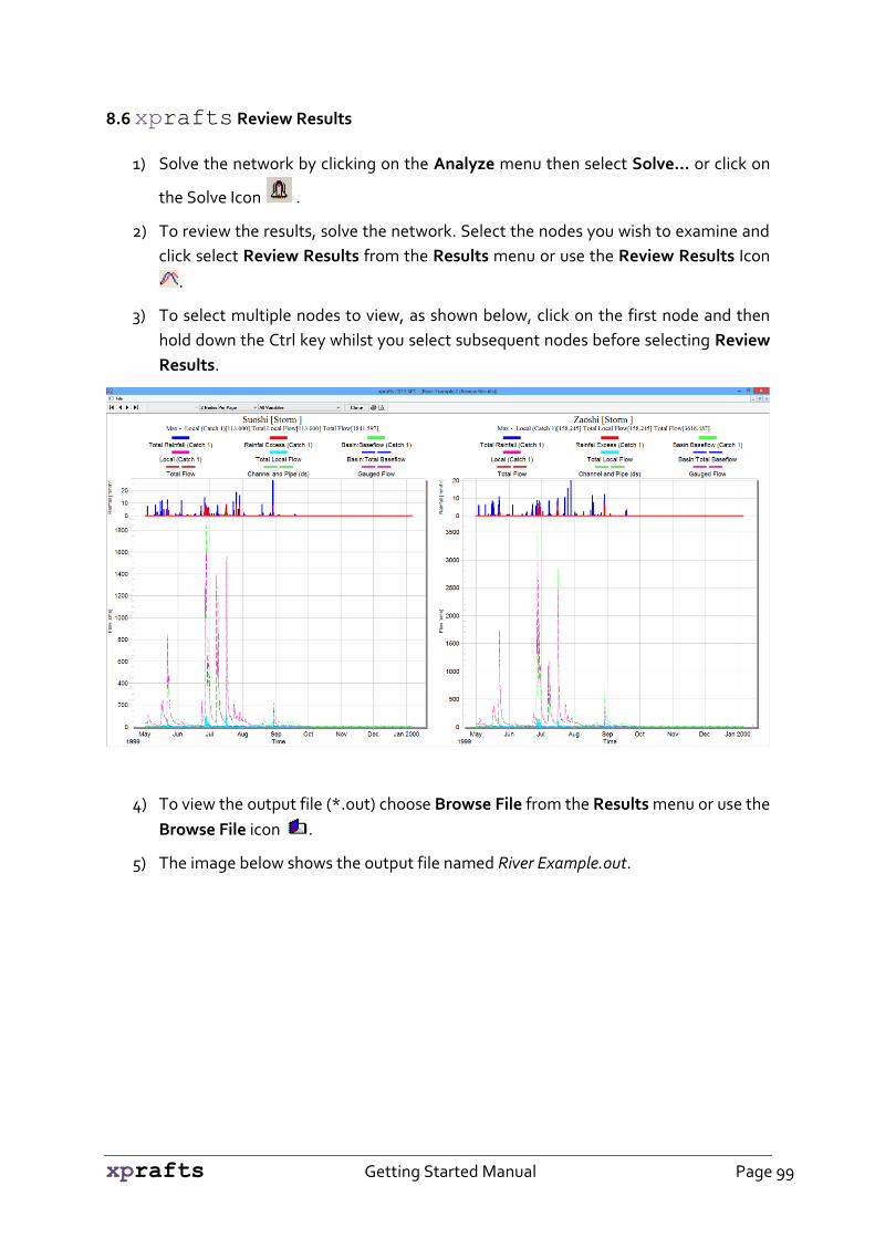
xprafts Getting Started Manual Page 99
8.6 xprafts Review Results
1) Solve the network by clicking on the Analyze menu then select Solve… or click on
the Solve Icon .
2) To review the results, solve the network. Select the nodes you wish to examine and
click select Review Results from the Results menu or use the Review Results Icon
.
3) To select multiple nodes to view, as shown below, click on the first node and then
hold down the Ctrl key whilst you select subsequent nodes before selecting Review
Results.
4) To view the output file (*.out) choose Browse File from the Results menu or use the
Browse File icon .
5) The image below shows the output file named River Example.out.
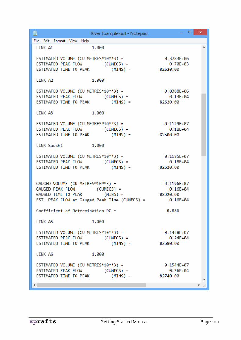
xprafts Getting Started Manual Page 100

xprafts Getting Started Manual Page 101
Tutorial 9: Detention Basin Versus On Site Detention
9.1 Introduction
For this example, the files you will need are found in the folder
c:\xps\xprafts2013SP1\GettingStarted\Tutorial9\.
PostSubPond.xp
PostSubOSDs.xp
PostSubOSDsamded.xp
PostSubdivsion.xp
PreSubdivison.xp
PLAN12.dwg
This example primarily uses xprafts to indicate how to size either a community pond
(detention basin) and/or on site detention (OSD) within each allotment to maintain natural
flow peaks after the development of the subdivision. It is assumed in this example that
prior to the creation of the subdivision the total catchment was natural and vegetated.
(Please Note: The sub-catchment areas upstream of the proposed subdivision have been
estimated here for purposes of the example. The sub-catchments throughout the subdivision
are also only rough estimates and may not exactly fit the real project).
Assumed Total Catchment Breakup
The example firstly sets up the model with nodes and links to represent locations where
potential OSD may be placed at the low point along the allotment boundary as well as the

xprafts Getting Started Manual Page 102
potential site for a community pond and then nodes to collect water from upstream sub-
catchments and roadway drains.
The screen capture above shows the suggested node/link layout with the imported
AutoCAD drawing of the proposed subdivision as a background. The background has been
utilised to position the nodes and links.
You can view the background by selecting background images from the View menu. Select
New and then click in the ellipses button. Select the PLAN12.DWG file and click on Open
and then OK.
To enlarge the image, select the zoom button .
Click and hold the mouse button down to draw a square around the part of the network you
wish to enlarge.
The aim is to do four runs:
Model 1: Pre Subdivision: All sub catchments are in their natural condition.
Model 2: Post Subdivision: Simply a copy of the pre-sub division model with the impervious
portions as the second sub-area to the appropriate nodes turned on by changing the
impervious % from 0 to 100
Model 3a Community Pond: Uses a small community pond at the outlet of the subdivision
contributing areas that also includes the central roadway.
Model 3b Post Sub division with OSDS: Uses only One Site Detention at each of the 9
allotments to achieve the same reduction. Note with the OSD the central roadway is not

xprafts Getting Started Manual Page 103
included and consequently OSD has to compensate for both the lot increases as well as the
un-retarded roadway increases.
9.2 Pre-Subdivision
1) Open the PreSubdivision.xp file.
2) The first model, seen below, is used without the background for clarity. This model
is for the pre sub divisional condition with all sub-catchments being in their natural
condition. The location of all nodes however is set in the critical post sub divisional
places.
3) The thick red lines represent the potential locations of post sub divisional OSDs
within each of the 9 lots. The thick black node represents the potential site for a
community pond that will collect all the water from the subdivision. The central line
of nodes represents road drainage once the subdivision is constructed. The road
areas that would be fully impervious would not be included in OSD capture, but
would be intercepted by the community pond.
4) The model also includes the total catchment upstream of subdivision to test the
effects of subdivision on total flow peak at the outlet (Cat Outlet).
(Please Note: The sub-catchment areas (hectares) are assumed for this example only
and do not accurately represents the site as shown).
The areas upstream of the proposed subdivision are assumed to be rural with sub-
catchment slopes of 1% and surface Manning’s roughness of 0.04.
The areas within the boundaries of the proposed subdivision are also assumed rural
pre-subdivision.

xprafts Getting Started Manual Page 104
When the subdivision is in place it is assumed that the central roadway is 100%
impervious and the areas within the allotments are 50% pervious and 50%
impervious.
The rural area sub-catchments upstream are coded with only sub-area to represent
total sub-catchment.
The sub-catchments representing the individual allotments are coded as split sub-
areas. The first area represents the pervious portion (0% impervious) and the
second area represents the impervious (100% impervious) portion. In the
PreSubdivision.xp model both sub-areas are coded as 0% impervious.
All models are using 60 minute combo rainfall, with a 10 year period assumed and
allow for multiple storms.
6) Job Control Including Storm Data: To examine job control data, including storm
data select Job Control from the Configuration menu.
7) If you click on the Global button you will be able to examine the stacked storms
dialog.

xprafts Getting Started Manual Page 105
8) To view the Storm Data for this example, click on the button labelled 10yr KL
Combo Storm in the Storm Type column.
9) With 10yr KL Combo Storm highlighted click on Edit.
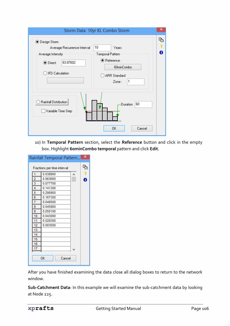
xprafts Getting Started Manual Page 106
10) In Temporal Pattern section, select the Reference button and click in the empty
box. Highlight 60minCombo temporal pattern and click Edit.
After you have finished examining the data close all dialog boxes to return to the network
window.
Sub-Catchment Data: In this example we will examine the sub-catchment data by looking
at Node 225.
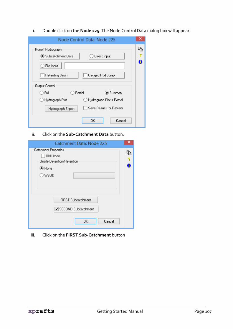
xprafts Getting Started Manual Page 107
i. Double click on the Node 225. The Node Control Data dialog box will appear.
ii. Click on the Sub-Catchment Data button.
iii. Click on the FIRST Sub-Catchment button

xprafts Getting Started Manual Page 108
iv. Click on OK when you have examined the data and then double click on the
SECOND sub catchment checkbox.
v. Click on OK.
Rainfall Loss/Infiltration Data: In this example we have assumed Initial Loss-Continuing
Loss rate.
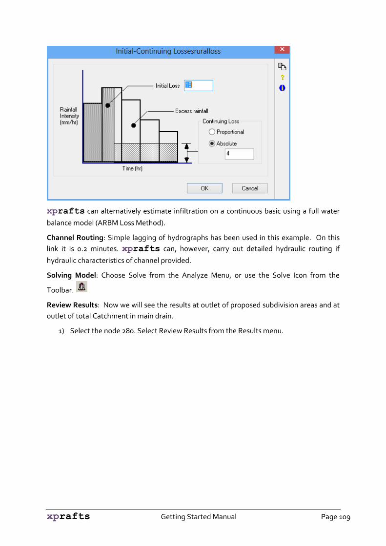
xprafts Getting Started Manual Page 109
xprafts can alternatively estimate infiltration on a continuous basic using a full water
balance model (ARBM Loss Method).
Channel Routing: Simple lagging of hydrographs has been used in this example. On this
link it is 0.2 minutes. xprafts can, however, carry out detailed hydraulic routing if
hydraulic characteristics of channel provided.
Solving Model: Choose Solve from the Analyze Menu, or use the Solve Icon from the
Toolbar.
Review Results: Now we will see the results at outlet of proposed subdivision areas and at
outlet of total Catchment in main drain.
1) Select the node 280. Select Review Results from the Results menu.

xprafts Getting Started Manual Page 110
2) Close the results window using the lower of the two crosses in the top right hand
corner. Select the node CatOut and select Review Results from the Results menu.
3) Close the results window and then select Close from the File menu to close the file.

xprafts Getting Started Manual Page 111
9.3 Post Subdivision
Open the file PostSubdivision.xp.
This model is simply a copy of the Pre Subdivisional model with the impervious portions as
the second sub-area to the appropriate nodes turned on by changing the impervious %
from 0 to 100.
The objectives of this model are to see how much the peak has increased at the potential
community basin site shown as larger thick black node, and in the main drain outlet that
collects water from the subdivision as well as upstream rural areas.
This will provide the information (i.e. the maximum pre subdivision peak discharge) that
the post development peak discharge needs to be reduced to.
Changes from Pre to Post Subdivisional Node Data:
1) Double click on node 225 to view the Node Control Data
2) Select Sub Catchment Data.
3) Click on the FIRST Sub-catchment button

xprafts Getting Started Manual Page 112
4) Click OK when you have examined the data, then click on the SECOND sub-
catchment button
5) Click on the Rainfall Losses button, label as Imploss in this example. With Imploss
highlighted in the Select dialog click on Edit.

xprafts Getting Started Manual Page 113
6) Close all windows and return to the network view.
Post Subdivision Results:
1) Click on the node 280 and select Review Result from the Results menu or use the
Review Results icon.
2) After you have examined the results click on the lower of the two crosses in the top
right hand corner to close the window and return to the network window.
3) Select the node 312 and review the results again.
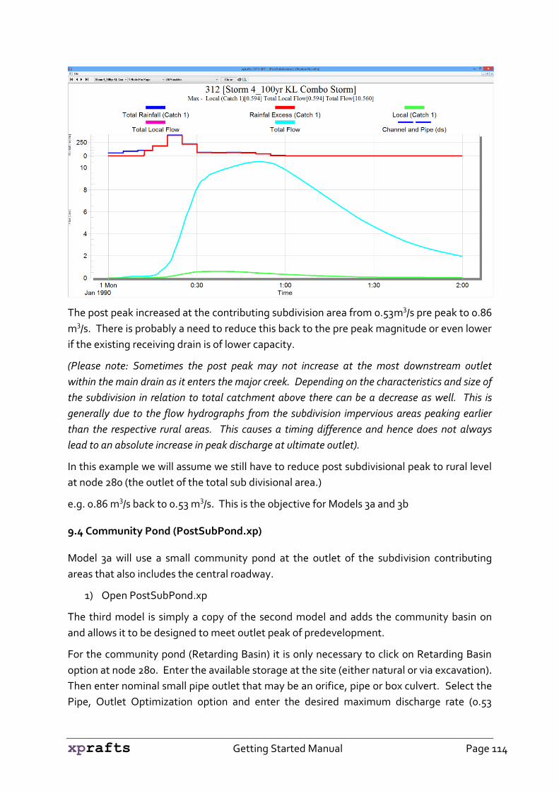
xprafts Getting Started Manual Page 114
The post peak increased at the contributing subdivision area from 0.53m3/s pre peak to 0.86
m3/s. There is probably a need to reduce this back to the pre peak magnitude or even lower
if the existing receiving drain is of lower capacity.
(Please note: Sometimes the post peak may not increase at the most downstream outlet
within the main drain as it enters the major creek. Depending on the characteristics and size of
the subdivision in relation to total catchment above there can be a decrease as well. This is
generally due to the flow hydrographs from the subdivision impervious areas peaking earlier
than the respective rural areas. This causes a timing difference and hence does not always
lead to an absolute increase in peak discharge at ultimate outlet).
In this example we will assume we still have to reduce post subdivisional peak to rural level
at node 280 (the outlet of the total sub divisional area.)
e.g. 0.86 m3/s back to 0.53 m3/s. This is the objective for Models 3a and 3b
9.4 Community Pond (PostSubPond.xp)
Model 3a will use a small community pond at the outlet of the subdivision contributing
areas that also includes the central roadway.
1) Open PostSubPond.xp
The third model is simply a copy of the second model and adds the community basin on
and allows it to be designed to meet outlet peak of predevelopment.
For the community pond (Retarding Basin) it is only necessary to click on Retarding Basin
option at node 280. Enter the available storage at the site (either natural or via excavation).
Then enter nominal small pipe outlet that may be an orifice, pipe or box culvert. Select the
Pipe, Outlet Optimization option and enter the desired maximum discharge rate (0.53

xprafts Getting Started Manual Page 115
m3/s). The output from the model will provide the required outlet size and the maximum
storage to limit the outlet flow peak to the specified target or slightly below.
(Please Note: It is alternatively possible to optimise the Pond to only use a particular available
storage by clicking on Maximum Storage button and entering the target storage in m3).
2) Solve the model using the Solve icon or by selecting Solve from the Analyze menu.
3) The required storage is 43.8 m3 and the maximum depth in the Pond is 0.51 m.
4) Discharge target was reached with 3 X 600mm dia pipes. This result is given at the
end of the PostSubPond.OUT file via the notebook editor icon on the xprafts tool
strip.
Double click on node 280 to open the Node Control Data dialog box. Double click on the
Retarding Basin button.

xprafts Getting Started Manual Page 116
There are many options in the Pond Retarding Basin Module in xprafts. To view the
different options click on the buttons to open their respective dialog boxes as seen below.
It is possible to add one or multiple spillways to act with larger storage storms, say 100 year
return period.
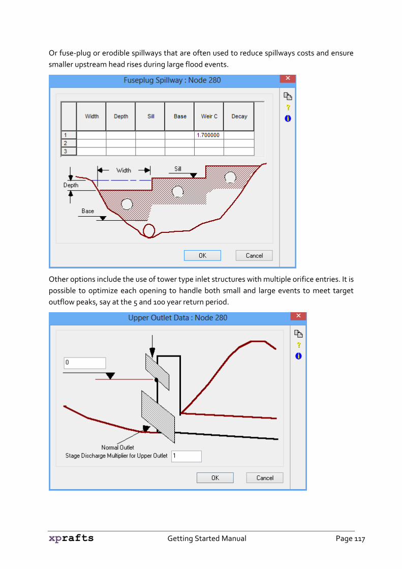
xprafts Getting Started Manual Page 117
Or fuse-plug or erodible spillways that are often used to reduce spillways costs and ensure
smaller upstream head rises during large flood events.
Other options include the use of tower type inlet structures with multiple orifice entries. It is
possible to optimize each opening to handle both small and large events to meet target
outflow peaks, say at the 5 and 100 year return period.

xprafts Getting Started Manual Page 118
Other outlet options include infiltration through Pond Bottom soil strata and evaporation
from the pond surface. This allows the addition of Retention to your Community Pond or
OSDs.
Retention basins as OSD or Community Ponds using combinations of infiltration,
evaporation and water reuse can be advantageous over traditional outlets – as they can
reduce development increases in runoff volume back to natural conditions as well as peaks.
xprafts can apply long term historical rainfall on a continuous basis to assess and
design acceptable retention structures to meet community safety and maintenance
requirements.
xprafts also allows the situation where there are multiple Ponds that may hydraulically
interact to affect the upstream stage/discharge characteristics dependent on the levels in
the respective Ponds.

xprafts Getting Started Manual Page 119
The model can be run over time periods of single storms up to many years and can be
calibrated to gauged data when available. This can allow analysis of how often Ponds fill
and how long they take to empty. This can be used in the assessment of maintenance and
multiple uses of normally dry pond areas for sporting areas etc. xprafts is currently
being used for flood forecasting as it is in China and rivers systems in Australia.
5) Close the file when you are finished.
9.5 Post Subdivision with OSDs
Model 3b use only On Site Detention at each of the 9 allotments to achieve the same
reduction. (Note that with the OSD the central roadway is not included and consequently
OSD has to compensate for both the increased lot discharges as well as the non retarded
roadway increases).
1) Open the PostSubOSDs.xp file.

xprafts Getting Started Manual Page 120
2) This model does not use the Community Pond to reduce flows to natural from the
subdivision area but instead uses OSDs within each of the 9 allotments. The
following OSD data is added to each of the allotment nodes.
3) Double Click on node 304 to open the Node Control Data dialog box.
4) Click Sub-Catchment Data button.

xprafts Getting Started Manual Page 121
5) Click on the button labelled Subdivision density.
6) With Subdivision density still highlighted click Edit.

xprafts Getting Started Manual Page 122
Note: In this example the allotment storage SSR and Maximum Site discharge PSD are
expressed as m3/ha and l/s/ha respectively. In this way each allotment in the subdivision is
treated equally according to their contributing area.
7) Close all windows and dialogs and return to the network window.
The SSR and PSD are iteratively estimated to cause correct peak discharge at the
subdivision outlet (at location of potential ponds) equal to the natural flow peak of 0.53
m3/s, or lower.
In this example the On-site Detention option is selected at each allotment at the low point
nodes. Further information is given to define the total impervious proportions within the
sub-catchment and the % capture of each into the OSD.
It should be noted here that the roadway does not get captured into the OSD that is located
in private property. This is normal for OSDs.
It is not necessary to have a node at each allotment as in this example. In other examples
urban sub-catchments have contained up to 1000 allotments. The OSDs will be allocated
to all the allotments in the sub-catchment.
8) Solve the model
9) Highlight Node 280 and select Review Results.

xprafts Getting Started Manual Page 123
The peak at potential Community Pond is 0.526m3/s with OSDs having SSR of 170 m3/ha
and PSD of 80 litres/s/ha.
It would also be possible to mix smaller ponds to optimise design of the total system. If
OSDs were adopted in place of the Community Pond at the outlet then it would also be
possible to simply run the outlets from the top four allotments directly into the existing
perimeter drain. In this way we do not have to bring their outputs back to the potential
pond site as indicated below.
If OSDs were adopted in place of the Community Pond at the outlet then it would also be
possible to simply run the outlets from the top four allotments directly into perimeter drain
that is already there and not drag their outputs back to potential pond site as indicated
below.
Rainwater Tanks
10) The OSD solution can also be further modified where excess capacity within roof
water tanks is now being utilised as part of the OSD solution.
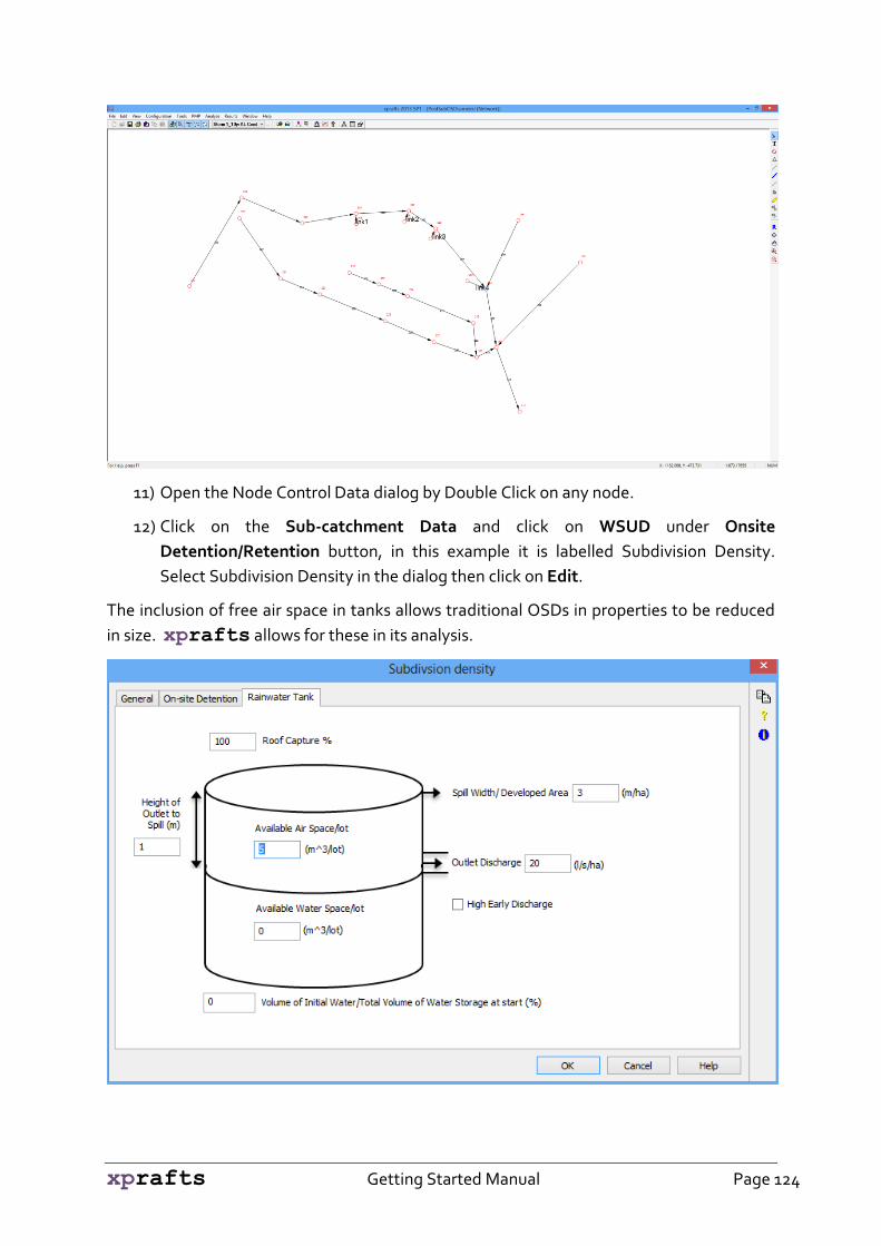
xprafts Getting Started Manual Page 124
11) Open the Node Control Data dialog by Double Click on any node.
12) Click on the Sub-catchment Data and click on WSUD under Onsite
Detention/Retention button, in this example it is labelled Subdivision Density.
Select Subdivision Density in the dialog then click on Edit.
The inclusion of free air space in tanks allows traditional OSDs in properties to be reduced
in size. xprafts allows for these in its analysis.
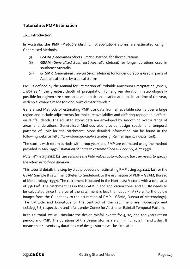
xprafts Getting Started Manual Page 125
Tutorial 10: PMP Estimation
10.1 Introduction
In Australia, the PMP (Probable Maximum Precipitation) storms are estimated using 3
Generalised Methods:
(i) GSDM (Generalised Short Duration Method) for short durations,
(ii) GSAM (Generalised Southeast Australia Method) for longer durations used in
southeast Australia
(iii) GTSMR (Generalized Tropical Storm Method) for longer durations used in parts of
Australia affected by tropical storms.
PMP is defined by the Manual for Estimation of Probable Maximum Precipitation (WMO,
1986) as "...the greatest depth of precipitation for a given duration meteorologically
possible for a given size storm area at a particular location at a particular time of the year,
with no allowance made for long-term climatic trends."
Generalised Methods of estimating PMP use data from all available storms over a large
region and include adjustments for moisture availability and differing topographic effects
on rainfall depth. The adjusted storm data are enveloped by smoothing over a range of
areas and durations. Generalised Methods also provide design spatial and temporal
patterns of PMP for the catchment. More detailed information can be found in the
following website (http://www.bom.gov.au/water/designRainfalls/pmp/index.shtml).
The storms with return periods within 100 years and PMP are estimated using the method
provided in ARR 1997 (Estimation of Large to Extreme Floods – Book Six, ARR 1997).
Note: While xprafts can estimate the PMP values automatically, the user needs to specify
the return period and duration.
This tutorial details the step by step procedure of estimating PMP using xprafts for the
GSAM Sample B catchment (Refer to Guidebook to the estimation of PMP – GSAM, Bureau
of Meteorology, 1997). The catchment is located in the Northeast Victoria with a total area
of 436 km2. The catchment lies in the GSAM Inland application zone, and GSDM needs to
be calculated since the area of the catchment is less than 1000 km² (Refer to the below
images from the Guidebook to the estimation of PMP – GSAM, Bureau of Meteorology).
The Latitude and Longitude of the centroid of the catchment are: 36deg19’S and
146deg36’E, respectively and it falls under Zone2 for Australian Rainfall Temporal Pattern.
In this tutorial, we will simulate the design rainfall events for 5, 20, and 100 years return
period, and PMP. The durations of the design storms are 15 min, 1 hr, 2 hr, and 1 day. It
means that 4 events x 4 durations = 16 design storms will be simulated.

xprafts Getting Started Manual Page 126
Figure 9.1. Generalised Method Zones for GSAM and GTSMR, (Source: The Estimation of Probable Maximum Precipitation in Australia: Generalised Southeast Australia Method – Bureau of Meteorology)
Figure 9.2. GSDM (Source: Guidebook to the Estimation of Probable Maximum Precipitation: Generalised Southeast Australia Method – Bureau of Meteorology)
14
6D
eg
30
min
E
36Deg19min S
Figure 9.3. Location of the catchment (Image from Google Earth)
The data/files supplied to complete this tutorial are:

xprafts Getting Started Manual Page 127
File Name Type Description
Aerial_Image.jpg Image file Aerial image of the project area
Aerial_Image.jpw World coordinate file File associated with the image file
PMP.xpt XP Template fileWhich contains temporal pattern for PMP, default job
control settings, global databases etc
Catchment_B_Extent.xpx XPX file Contains the extent of the catchment B
Note: users can use the *.shp, *.dwg, *.dxf, or image files to digitize the catchments.
10.2 Create File from Template
First we need to create the file using the PMP.xpt template.
Open xprafts, go to File\New\Create from Template. Name the model PMP.xp and
Save in the desired location.
Now xprafts asks you to select the template in the Template folder in the installed
directory by default. Choose the template named PMP.xpt and click on Open.
The PMP.xpt file contains the GSDM, GSAM, and GTSMR temporal patterns and the IFD
data for the study area.
10.3 Load Background Image and Catchment Extent
Add new background image Aerial_Image.jpg (Refer to as in Tutorials 5 (section 5.2)). Then
load the catchment extent called Catchment_B_Extent.xpx by going to File\Import Data,

xprafts Getting Started Manual Page 128
browse for the file and Open it. In this example the catchment has been made available for
the training purpose. Users will need to create the catchment, if it is not made available,
using the Create Subcatchment Tool or go to the PMP menu in the main menu, select
Catchment Extent, then Create, and digitize the catchment. You will need define the
whole catchment as well as sub-catchments as represented in the following section.
10.4 Creating Subcatchments
Now digitize three sub-catchments as shown using the Create Subcatchment Tool .
Alternatively, you can add *.shp, *.mif, *.dwg files as catchment background images and
digitize the catchments using the Create Subcatchment Tool.

xprafts Getting Started Manual Page 129
10.5 Create catchment collection points
Add nodes in the catchments outlet points using Node Tool , then connect these nodes
(from Node 1 to Node 3) using Link Tool .
Now we will connect the catchments to the outlet nodes. Make sure that the Lock
Catchments Tool is switched-off as connecting the catchments to the collection
points. Select Pointer Tool and Left Click on the catchment, you will see that the
Cursor has changed as shown in the image below. Keep the Left Button pressed and release

xprafts Getting Started Manual Page 130
it when the cursor reaches the outlet node. Select the Drain Catchment As
\Subcatchment1.
Repeat this step for all the other catchments.
Now, select all the nodes by clicking on the Select all nodes Tool . Go to Tools Menu,
select Calculate Node and click on Catchment Area.

xprafts Getting Started Manual Page 131
You can see that the catchment areas are calculated and assigned as FIRST Subcatchment
to the nodes.
Double Click on any node to open Node Control Data and select Subcatchment Data, and
click on FIRST Subcatchment button. You can see that the calculated area is assigned in
Total Area to the node.
Double Click on link 1 to open Link Lagging and enter Lag as 200 min. Similarly, Lag for link
2 is entered as 350 min.
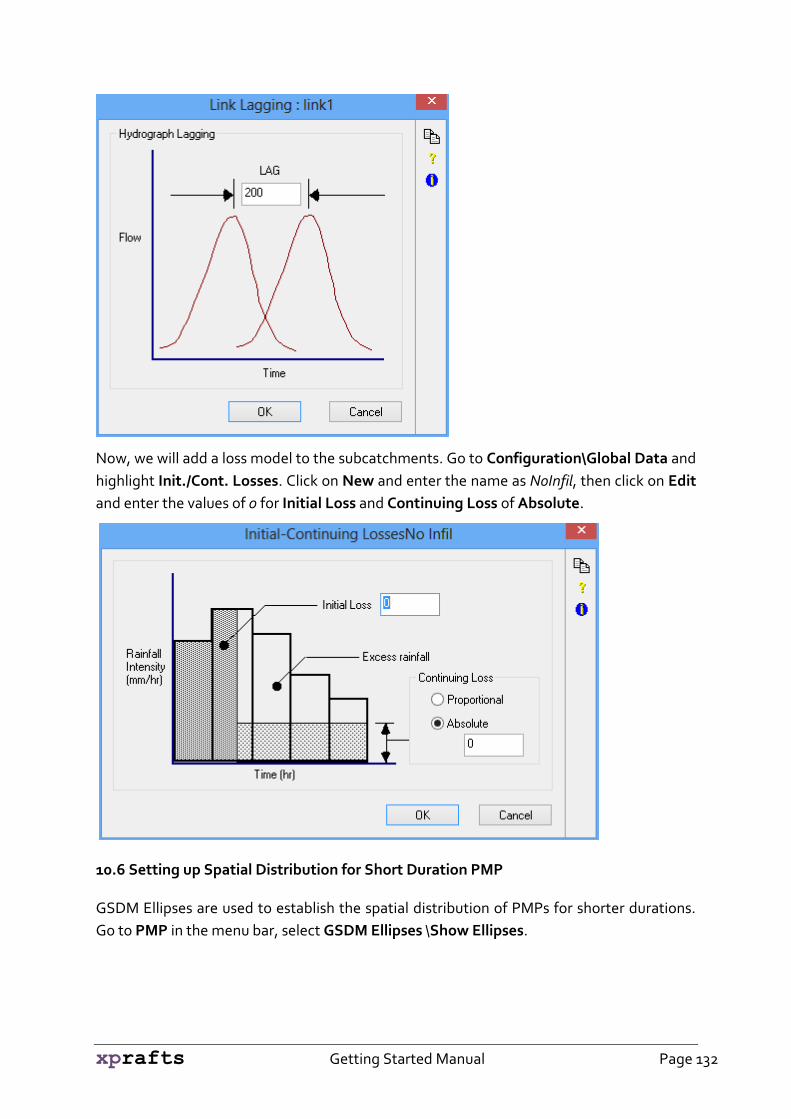
xprafts Getting Started Manual Page 132
Now, we will add a loss model to the subcatchments. Go to Configuration\Global Data and
highlight Init./Cont. Losses. Click on New and enter the name as NoInfil, then click on Edit
and enter the values of 0 for Initial Loss and Continuing Loss of Absolute.
10.6 Setting up Spatial Distribution for Short Duration PMP
GSDM Ellipses are used to establish the spatial distribution of PMPs for shorter durations.
Go to PMP in the menu bar, select GSDM Ellipses \Show Ellipses.

xprafts Getting Started Manual Page 133
You will see the 10 ellipses on the screen now (A – J) and the center point of the ellipses as a
small circle. The next step is to overlay the ellipses with the catchment outline by moving
and rotating to obtain the best fit by the smallest possible ellipse. To do this, click on the
Center Circle of the ellipses and hold Left mouse. Now you will be able to move the ellipses.
To rotate the ellipses, press Shift on the key board.
While moving and rotating the ellipses, you are able to see the PMP Monitor dialogue
which shows the GSDM spatial distribution calculations. To see this monitor click on PMP
from the menu bar, select GSDM Ellipses \Show PMP Calculations.
Then go to PMP\GSDM Ellipses and tick on Lock Ellipses. You can see that the ellipses are
locked and cannot be moved.
You can lock the nodes and catchments as well using the tools respectively.

xprafts Getting Started Manual Page 134
10.7 Automated Storm Generation
Automatic Storm Generator is used for generating storms with any storm durations with
any return periods. Storms up to 100 years return period is estimated using the IFD
coefficients, rainfall duration, and temporal pattern depending upon the zone (Reference:
AR&R 1987).
To activate the Automatic Storm Generator, go to Configuration\Job Control.
Alternatively click on Job Control Icon and select Job Definition. Tick on the Automatic
Storm Generator radio button.
Now you can see the Global Storm Generator dialogue. Click on the Global Storms tab.

xprafts Getting Started Manual Page 135
Click on IFD and select the global database for IFD coefficients called Albury. The Albury
data was included in the template file PMP.xpt and represents the IFD coefficients for the
region. Click on Edit and you can see the IFD coefficients for the project area.

xprafts Getting Started Manual Page 136
Note: You can get these IFD coefficients from the ARR 1987, Volume 2. Design rainfall
isopleths’ maps are available for 2 and 50 years for 1, 12, and 72 hours durations. Location
skewness and geographical factors also available in the ARR volume. Otherwise, you can get
these coefficients from the Australian Bureau of Meteorology website:
http://www.bom.gov.au/hydro/has/cdirswebx/cdirswebx.shtml.
Click on OK and highlight Albury and click on Select in the next dialogue box.
In the Global Storm Generator dialog enter the Zone as 2 as the study area is under zone 2
of the Australian rainfall temporal pattern. Refer to the figure given by ARR 1987 as below:
Figure 9.4. Design Rainfall Temporal Pattern Zones for Australia – Source: ARR 1987, BOM.
In the Global Storm Generator dialog, under Time Control, enter Routing Increment as 1
min; under Simulation Time enter Simulation Time = Storm Duration x 1. Next, tick on
the Storm Duration of 15, 60, 120, and 1440 min and select Return Period of 5, 20, 100, and
PMP.
Note: when you tick on PMP as return period, 10, 20, 25 min Storm Durations will be greyed
out automatically as PMPs will not be calculated for these durations.
Now xprafts will calculate 4 events x4 durations = 16 design storms chosen for the
catchment.
The temporal patterns up to 100 year return period are stored in the program. The engine
will pick up the corresponding temporal pattern for a storm depending upon the zone,
return period, and duration. However, the temporal patterns for the PMP should be
specified by users. For GSDM there will be a single temporal pattern (up to 3 or 6 hours).

xprafts Getting Started Manual Page 137
Figure 9.5. Temporal Pattern for PMP for short durations (Source: the Estimation of Probable Maximum Precipitation in Australia: Generalised Short-Duration Method, BOM, 2003)
There are different temporal patterns for GSAM and GTSMR depends upon the catchment
area and storm duration. The temporal pattern for GSAM and GTSMR are starting from 24
hours. The user should estimate the in-between values (3-24 hours) as described in the
GSAM and GSTMR Guidebooks from Bureau of Meteorology.
10.8 Setting up GSDM Data for Shorter Duration Storms
Open Job Control\Automatic Storm Generator and select the PMP tab. You can see that
the Total Area of the catchment is automatically calculated. Now enter Latitude of -360 19’
and Longitude of 1460 36’ for the catchment centroid. These values will be used in
calculation of adjustment factors for GSAM and/or GTSMR. Enter PMP Return Period of
1000000 years. Note: data will be used to interpolate values between 100 years and PMP (say,
150 or 200 year return period).
Under GSDM- Generalized Short Duration Method select Duration Limit as <3 hr from
the dropdown list. Click on Temporal Pattern and select GSDM from the global database
imported from the PMP.xpt, click on Select. Note that there is only one temporal pattern for
the short duration PMP estimation that is GSDM .

xprafts Getting Started Manual Page 138
Now click on GSDM Worksheet to open Global Storms Summary for GSDM and enter the
following values:
Smooth (S) (smooth fraction of terrain) as 0, EAF as 1, and MAF as 0.60.
Note: refer to the Estimation of Probable Maximum Precipitation in Australia: Generalised
Short-Duration Method (BOM, 2003) for more details about terrain types and adjustment
factors. Paragraph below is cited in the guidebook:
“Rainfall from single, short duration thunderstorm events is not significantly affected by the
terrain. Therefore, it is not necessary to classify the terrain of the catchment for durations of
an hour or less. If durations longer than one hour are required, the next step is to establish the
terrain category of the catchment and to calculate the percentages of the catchment that are
‘rough’ and ‘smooth’. ‘Rough’ terrain is classified as that in which elevation changes of 50 m or
more within horizontal distances of 400 m are common. ‘Rough’ terrain induces areas of low
level convergence which can contribute to the development and redevelopment of storms,
thereby increasing rainfall in the area over longer durations. Terrain that is within 20 km of
generally ‘rough’ terrain should also be classified as ‘rough’. If there is ‘smooth’ terrain within
the catchment that is further than 20 km from generally ‘rough’ terrain, an areally weighted

xprafts Getting Started Manual Page 139
factor of ‘rough’ (R) and ‘smooth’ (S) terrain should be calculated such that R plus S equals
one. If a catchment proves difficult to classify under these guidelines then the whole
catchment should be classified as ‘rough’
“The mean elevation of the catchment should be estimated from a topographic map. If this value is less than or equal to 1500 m the EAF is equal to one. For elevations exceeding 1500 m the EAF should be reduced by 0.05 for every 300 m by which the mean catchment elevation exceeds 1500 m. For most catchments in Australia the EAF will be equal to one.”)
Figure 26 - Moisture Adjustment Factor. Source: GSDM Guidebook, BOM
Click on Update under the GSDM tab from Global Storms Summary. You see that the
GSDM PMP depths are estimated from Equation (in the PMP Values (mm) table) up to 3
hours as we specify the duration limit to < 3 hrs.
Note that Initial Depth Smooth (Ds) in the PMP Values (mm) table for the Smooth Terrain
calculated are 0.
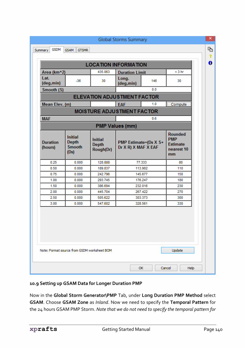
xprafts Getting Started Manual Page 140
10.9 Setting up GSAM Data for Longer Duration PMP
Now in the Global Storm Generator\PMP Tab, under Long Duration PMP Method select
GSAM. Choose GSAM Zone as Inland. Now we need to specify the Temporal Pattern for
the 24 hours GSAM PMP Storm. Note that we do not need to specify the temporal pattern for
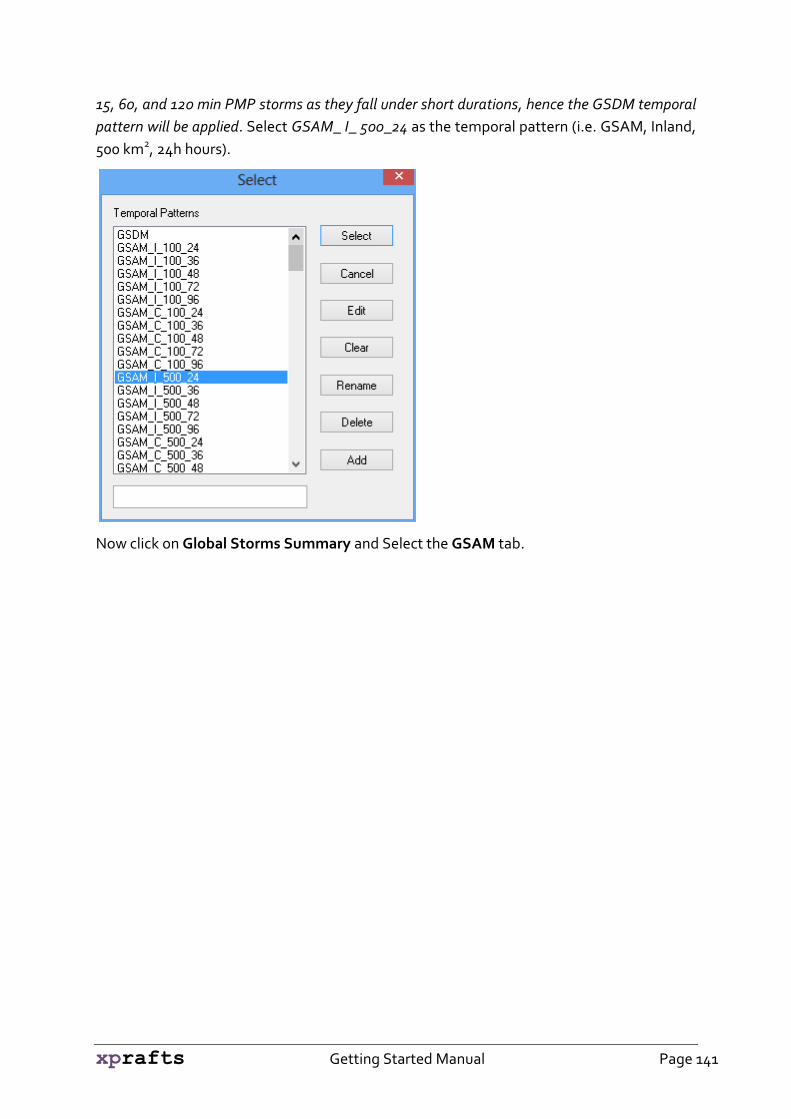
xprafts Getting Started Manual Page 141
15, 60, and 120 min PMP storms as they fall under short durations, hence the GSDM temporal
pattern will be applied. Select GSAM_ I_ 500_24 as the temporal pattern (i.e. GSAM, Inland,
500 km2, 24h hours).
Now click on Global Storms Summary and Select the GSAM tab.

xprafts Getting Started Manual Page 142
Under CATCHMENT FACTORS click on Compute for Topographic Adjustment Factor
(TAF) and TAF will be calculated based on the entered latitude and longitude.
Similarly, click on Compute for EPW Seasonal catchment average to calculate for
Summer and Autumn. Alternatively, you can directly enter the values of TAF and EPW.
Note that xprafts calculates the TAF and EPWs values based on the latitude and
longitude of the catchment centroid. It will be more accurate if the average value for the
catchment is calculated by overlaying the catchment outline on the TAF and EPWs grids as
described in the GSAM Guidebook.
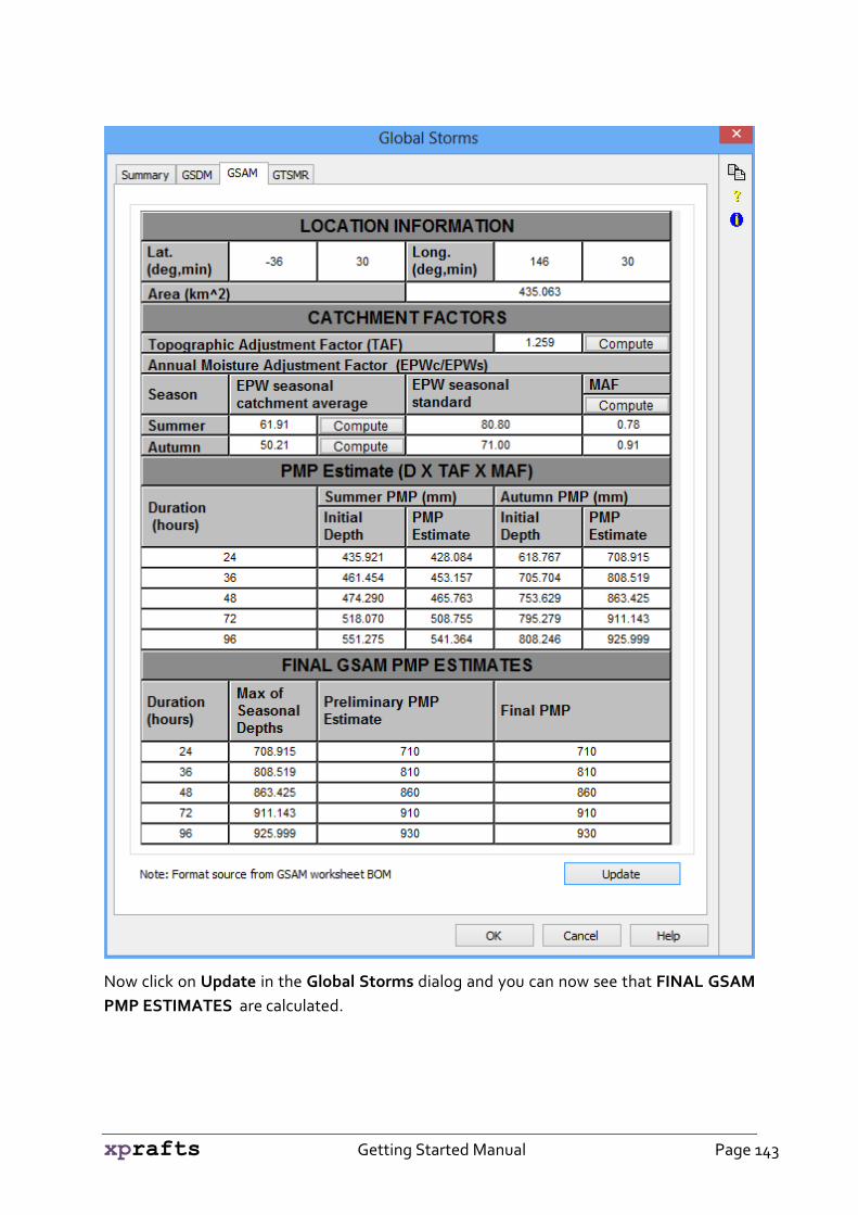
xprafts Getting Started Manual Page 143
Now click on Update in the Global Storms dialog and you can now see that FINAL GSAM
PMP ESTIMATES are calculated.

xprafts Getting Started Manual Page 144
10.10 Setting up GTSMR Data for Longer Duration PMP
Note that for Catchment B the GTSMR estimation is not required. However, for some other
catchments GTSMR estimation will be required based on the location and the user can follow
the same procedure that is provided for the GSAM. For some catchments both GSAM and
GTSMR will be applicable, e.g. GSAM-GTSMR Coastal Transition Zone. In that case, the PMP
depths should be estimated by both the methods and the maximum value is selected.
10.11 Analysis and Results
Click on Solve to simulate the model. To review results, select the nodes that you wish to
see the results and click on Review Results.

![Flood Forecasting During Major Flood Events: The 2011 ......• Manitoba Antecedent Precipitation Index (MANAPI) Runoff = f(SMI,PRECIP [Snow+Rain]) • Unit Graph + Muskingum routing](https://static.fdocuments.us/doc/165x107/6134d50ddfd10f4dd73bfbbb/flood-forecasting-during-major-flood-events-the-2011-a-manitoba-antecedent.jpg)