Unsupervised Learning for Matrix Decompositions - HIIT Learning Coffee... · Unsupervised Machine...
48
Unsupervised Machine Learning for Matrix Decomposition Erkki Oja Department of Computer Science Aalto University, Finland Machine Learning Coffee Seminar, Monday Jan. 9, HIIT
Transcript of Unsupervised Learning for Matrix Decompositions - HIIT Learning Coffee... · Unsupervised Machine...
Unsupervised Machine Learning for Matrix
Decomposition
Erkki Oja
Department of Computer Science
Aalto University, Finland
Machine Learning Coffee Seminar, Monday Jan. 9, HIIT
Matrix Decomposition
• Assume three matrices A, B, and C
• Consider equation
A = BC
• If any two matrices are known, the third one
can be solved
• Very dull. So what?

• But let us consider the case when only one (say, A) is known.
• Then A BC is called a matrix decomposition for A
• This is not unique but becomes very useful when suitable constraints are posed.
• Some very promising machine learning techniques are based on this.

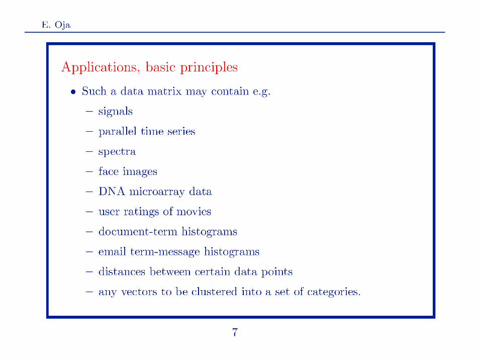
Example: spatio-temporal data
• Graphically, the situation may be like this:
space
space
time
time
A B
C

Global daily temperature (10.512 points x 20.440 days)
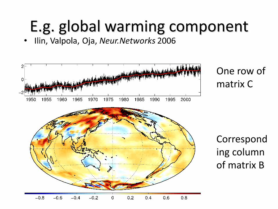
E.g. global warming component
One row of matrix C
Corresponding column of matrix B

More formally:

jx
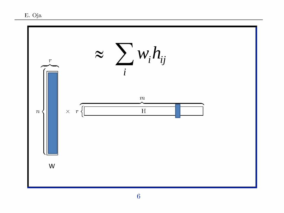
ij
i
ihw
W

Principal Component Analysis (PCA)


(Gradient descent and neural networks: Oja, J.Math.Biol. 1982)

Example First Principal Comp. of climate data: Global air pressure

• To recapitulate, Principal Component Analysis means
• where matrix W has orthogonal columns.
• Approximation by squared matrix norm.
XWWX T
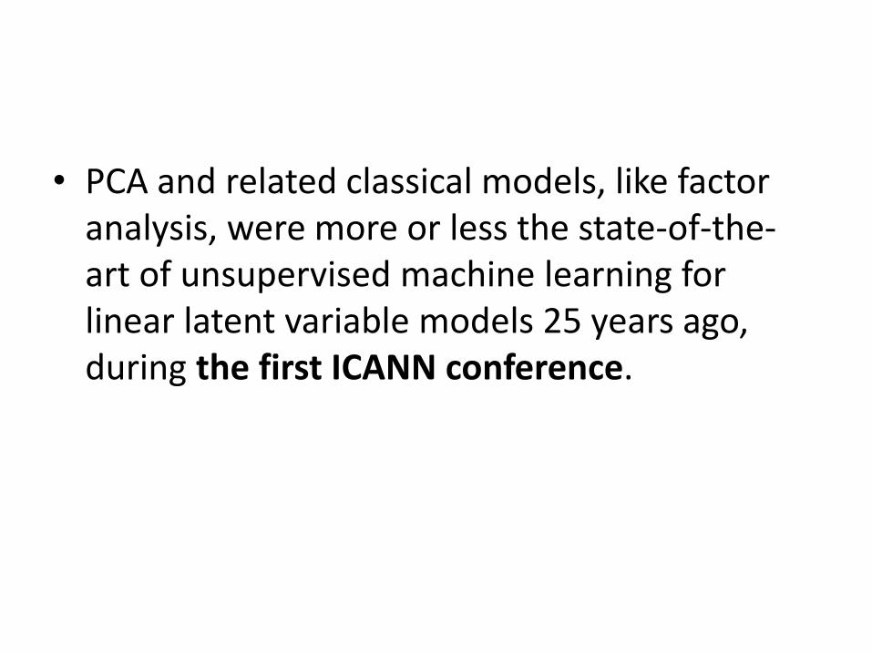
• PCA and related classical models, like factor analysis, were more or less the state-of-the-art of unsupervised machine learning for linear latent variable models 25 years ago, during the first ICANN conference.

The first ICANN ever, in 1991

• My problem at that time: what is nonlinear PCA ?
• My solution: a novel neural network, deep auto-encoder
• E. Oja: Data compression, feature extraction, and auto-association in feedforward neural networks. Proc. ICANN 1991, pp. 737-745.

Deep auto-encoder (from the paper)

• The trick is that a data vector x is both the input and the desired output.
• This was one of the first papers on multilayer (deep) auto-encoders, which today are quite popular.
• In those days, this was quite difficult to train.
• Newer results: Hinton and Zemel (1994), Bengio (2009), and many others.
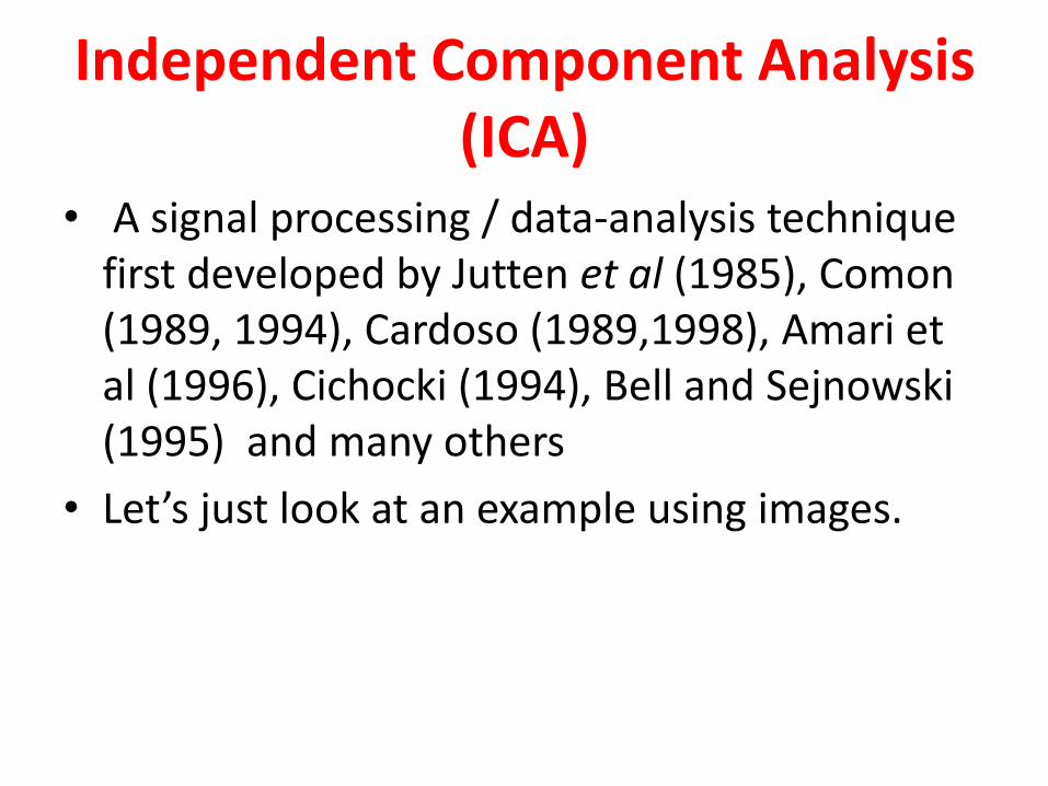
Independent Component Analysis (ICA)
• A signal processing / data-analysis technique first developed by Jutten et al (1985), Comon (1989, 1994), Cardoso (1989,1998), Amari et al (1996), Cichocki (1994), Bell and Sejnowski (1995) and many others
• Let’s just look at an example using images.

Original 9 “independent” images (rows of matrix H)

9 mixtures with random mixing matrix W; these images are the rows of matrix X, and this is the only available data we have

Estimated original images, found by an ICA algorithm

• Pictures are from the book “Independent Component Analysis” by Hyvärinen, Karhunen, and Oja (Wiley, 2001)
• ICA is still an active research topic: see the Int. Workshops on ICA and blind source separation / Latent variable analysis and signal separation (12 workshops, 1999 – 2015)

• To recapitulate, Independent Component Analysis means
• where the rows of matrix H are statistically
independent.
WHX
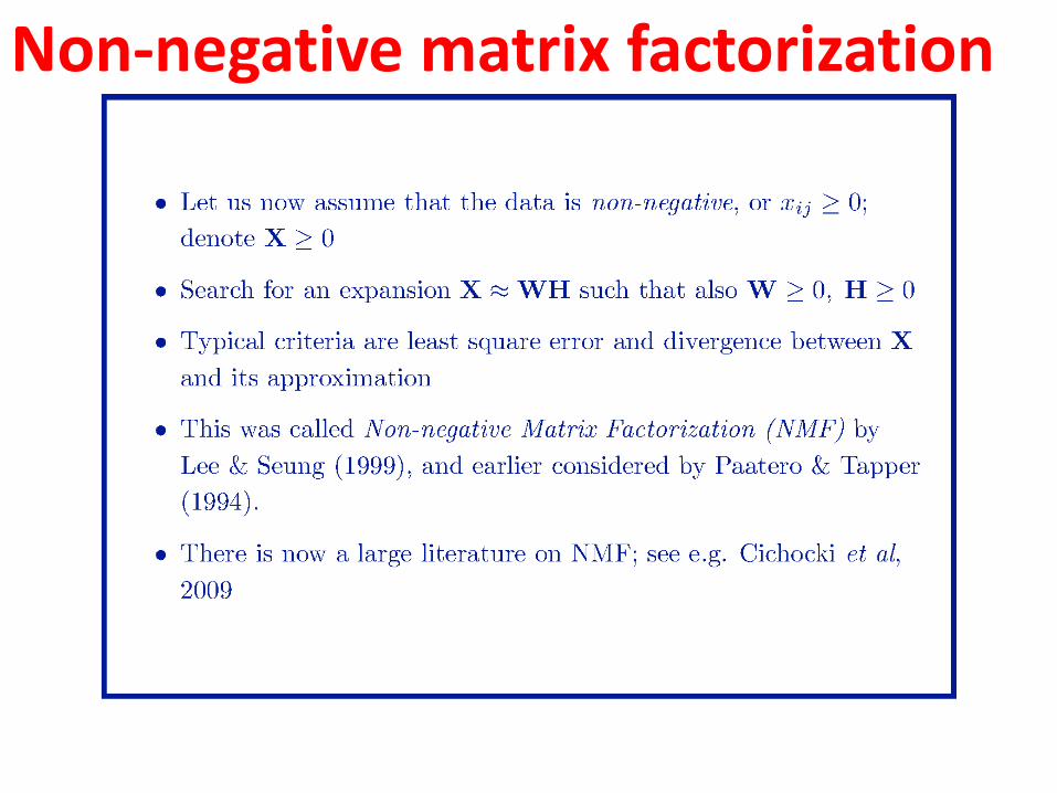
Non-negative matrix factorization

• NMF and its extensions is today quite an active research topic
– Tensor factorizations (Cichocki et al, 2009)
– Low-rank approximation (LRA) (Markovsky, 2012)
– Missing data (Koren et al, 2009)
– Robust and sparse PCA (Candés et al, 2011)
– Symmetric NMF and clustering (Ding et al, 2012)

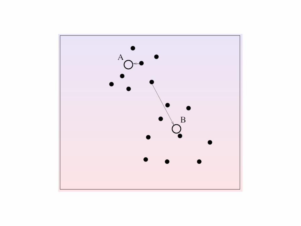
NMF and clustering
• Clustering is a very classical problem, in which n vectors (data items) must be partitioned into r clusters.
• The clustering result can be shown by the nxr cluster indicator matrix H
• It is a binary matrix whose element if and only if the i-th data vector belongs to the j-th cluster
1ijh


• The k-means algorithm is minimizing the cost function:
• If the indicator matrix is suitably normalized then this becomes equal to (Ding et al, 2012)
• Notice the similarity to NMF and PCA! (“Binary PCA”)
2
1
r
j Cx
ji
ji
cxJ
2TXHHXJ

• Actually, minimizing this (for H) is
mathematically equivalent to maximizing
which immediately allows the “kernel trick” of replacing with kernel , extending k-means to any data structures (Yang and Oja, IEEE Tr-Neural Networks, 2010).
)( TT XHHXtr
XX T ),( ji xxk
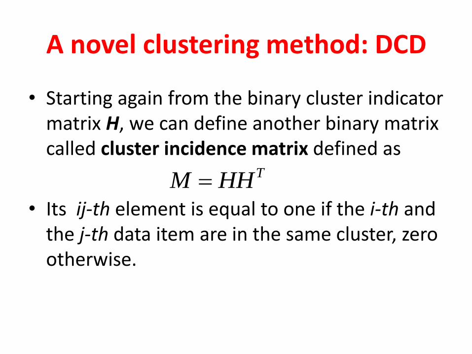
A novel clustering method: DCD
• Starting again from the binary cluster indicator matrix H, we can define another binary matrix called cluster incidence matrix defined as
• Its ij-th element is equal to one if the i-th and the j-th data item are in the same cluster, zero otherwise.
THHM

• It is customary to normalize it so that the row sums (and column sums, because it is symmetric) are equal to 1 (Shi and Malik, 2000). Call the normalized matrix also M.
• Assume a suitable similarity measure between every i-th and j-th data items (for example a kernel). Then a nice criterion is:
ijS
MSJ

• This is an example of symmetrical NMF because both the similarity matrix and the incidence matrix are symmetrical, and both are naturally nonnegative.
• S is full rank, but the rank of M is r.
• Contrary to the usual NMF, there are two extra constraints: the row sums of M are equal to 1, and M is a (scaled) binary matrix.
• The solution: probabilistic relaxation to smooth the constraints (Yang, Corander and Oja,
JMLR, 2016)
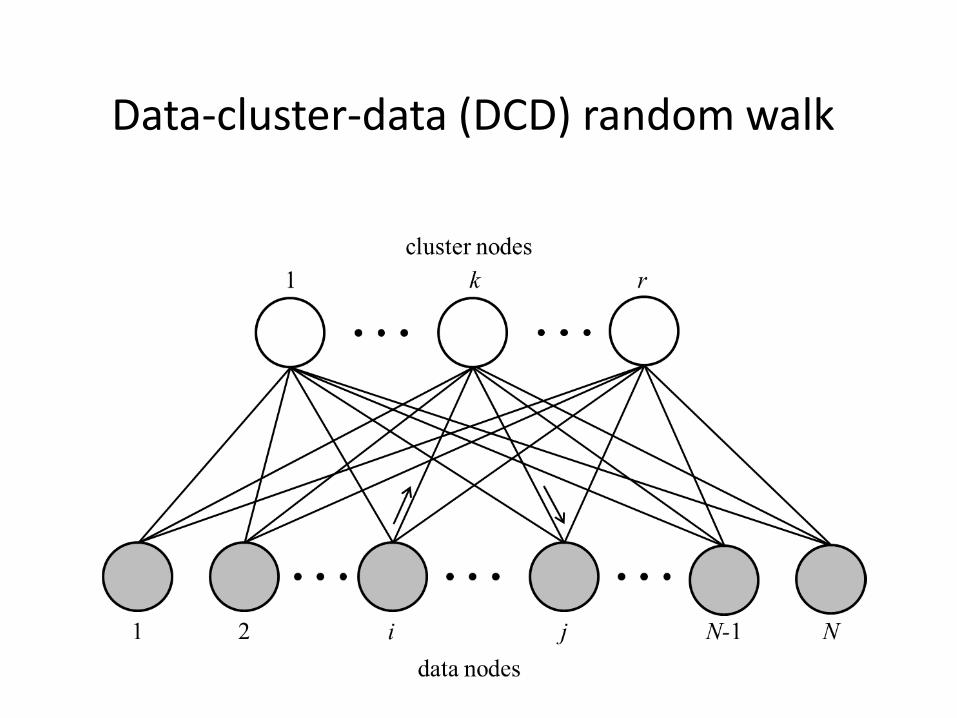
Data-cluster-data (DCD) random walk

Clustering results for large datasets
DCD k-means Ncut

Clustering results for large datasets
DCD k-means Ncut
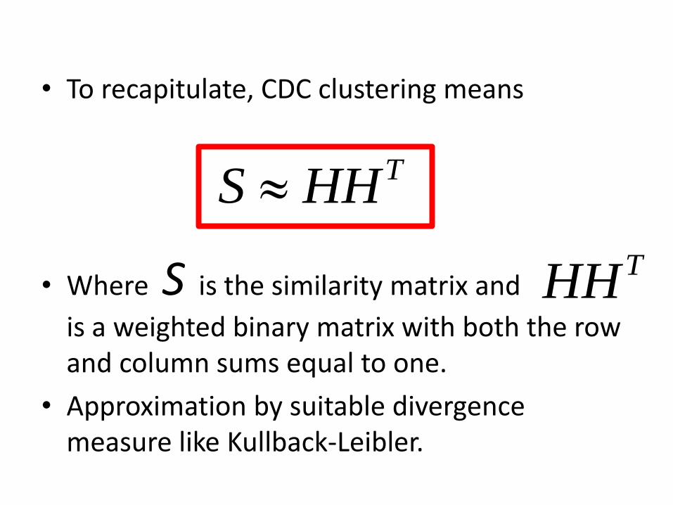
• To recapitulate, CDC clustering means
• Where S is the similarity matrix and
is a weighted binary matrix with both the row and column sums equal to one.
• Approximation by suitable divergence measure like Kullback-Leibler.
THHS
THH
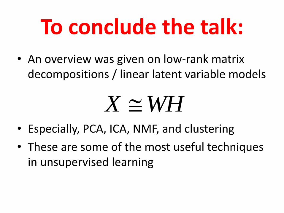
To conclude the talk: • An overview was given on low-rank matrix
decompositions / linear latent variable models
• Especially, PCA, ICA, NMF, and clustering
• These are some of the most useful techniques in unsupervised learning
WHX

• While such linear models seem deceivingly simple, they have some advantages:
– They are computationally simple
– Because of linearity, the results can be understood: the factors can be explained contrary to “black-box” nonlinear models such as neural networks
– With nonlinear cost functions and constraints, powerful criteria can be used.

THANK YOU FOR YOUR ATTENTION!

Additional material
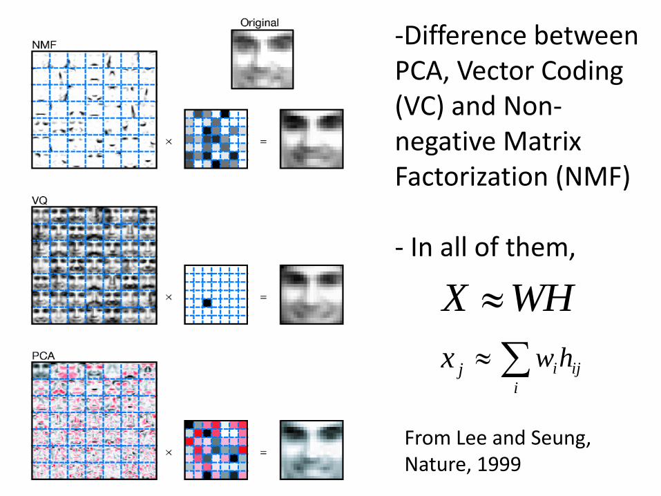
From Lee and Seung, Nature, 1999
-Difference between PCA, Vector Coding (VC) and Non-negative Matrix Factorization (NMF) - In all of them, WHX
jx ij
i
ihw


![Feature Learning with Matrix Factorization Applied to Acoustic … · 2016. 12. 4. · Victor Bisot, Romain Serizel, ... [21] by comparing popular unsupervised matrix factorization](https://static.fdocuments.us/doc/165x107/60d66ffc3229cb41555a25a3/feature-learning-with-matrix-factorization-applied-to-acoustic-2016-12-4-victor.jpg)