1/ Respectively, Professor, Research Assistant and Associate Professor of AgriculturalEconomics, University of Wisconsin-Madison. This research was supported in part by aHatch grant.

Copyright © 1994 by Jean-Paul Chavas, Michael Aliber, and Thomas L. Cox. All rights reserved. Readers may make verbatim copies of thisdocument for non-commercial purposes by any means, provided that this copyright notice appears on all such copies.

A NONPARAMETRIC ANALYSIS OF THE SOURCE

AND NATURE OF TECHNICAL CHANGE:

THE CASE OF U.S. AGRICULTURE

by

Jean-Paul Chavas

Michael Aliber

and

Thomas L. Cox1/

A NONPARAMETRIC ANALYSIS OF THE SOURCE AND NATURE OF TECHNICAL CHANGE:

THE CASE OF U.S. AGRICULTURE

I- Introduction:

Much research has been done on technical change and its economic significance. The

importance of technical change in economic growth is widely acknowledged (e.g., Solow,

1957). Yet, the process of technical change is quite complex and still poorly understood. It is

often described as a dynamic two-stage process: 1/ the creation of new knowledge and

technology; and 2/ the adoption of new technology by firms. For example, in his study of an

innovation cycle, Griliches (1957) identified significant lags between the creation of new

knowledge and the adoption of the associated new technology. The creation of new

knowledge is stimulated by expenditures on research and development (R&D). Because of

the cost of acquiring new knowledge and adapting it to local conditions, the adoption process

for a new technology can be slow. The lags between R&D investment and its payoff can vary

with each technology and each industry. However, as a rule, these lags are longer as the

research is more basic, and shorter as the research is more applied.

A distinction often made in the literature concerns the source of funding for R&D, i.e.,

public versus private. When new knowledge has the characteristics of a public good, then

public funding of research may be appropriate (e.g., Arrow, 1962). Alternatively, when

property rights to technology can be privately assigned and enforced (e.g., through patents),

then private institutions can have the proper incentive to invest in R&D. But because patent

rights expire at the end of the patent life, private incentives to invest in basic research with

longer term (and more uncertain) payoffs are weak. As a result, basic research tends to be

2

funded publicly, and private R&D tends to focus on applied research with shorter term

payoffs that can be appropriated during a patent life.

The linkage between technical change and resource scarcity has been the subject of

much scrutiny. By definition, technical progress allows the production of greater outputs with

the same amount of resources, or the use of fewer resources to produce the same outputs.

Thus, it can help reduce resource scarcity. The feedback effect of resource scarcity on

technical change is also of interest. It has been expressed in terms of "induced innovation".

As first suggested by Hicks, the induced innovation hypothesis states that relative resource

scarcity tends to guide the process of technical change:

A change in relative prices of the factors of production is itself a sign to invention, and

to invention of a particular kind -- directed to economising the use of a factor which

has become relatively expensive (Hicks, 1932).

The induced innovation hypothesis is typically formulated in terms of the bias in technical

change (e.g., see Binswanger and Ruttan, 1978). Roughly stated, technical change is said to

be biased toward a particular factor (or factor-using) if it stimulates the relative use of this

factor. Conversely, technical change is biased against a particular factor (or factor-saving) if

it reduces the use of this factor relative to other factors. In this context, the induced

innovation hypothesis predicts that technical change will be biased against a particular factor

(i.e., factor-saving) when this factor's relative scarcity (e.g., its relative price) increases.

Conversely, technical change will be biased in favor of a given factor (i.e., factor-using) when

its relative price declines.

The induced innovation hypothesis has been subject to empirical testing. Binswanger

3

(1974) and Hayami and Ruttan (1985) found empirical evidence in support of the hypothesis,

while Olmstead and Rhodes (1993) uncovered some historical evidence inconsistent with

induced innovation. This research has typically measured the bias in technical change and

compared its direction with changes in relative prices. The linkage between this bias and the

nature of invention has often not been made explicit. This is unfortunate, since Hicks's

original formulation of the induced innovation hypothesis explicitly mentions inventive

activities. This suggests a need to explore jointly the economics of R&D investments and

induced innovations. Given the dynamics of R&D effects, this indicates that induced

innovations should also be investigated in a dynamic setting.

The objective of this paper is to analyze the process of technical change with a joint

focus on the effects of R&D investments and on the induced innovation hypothesis. This is

done relying on nonparametric methods developed by Afriat (1972), Hanoch and Rothschild

(1972) and Varian (1984) (section II). The nonparametric approach to production analysis

consists in analyzing a finite body of data without ad hoc specification of functional forms for

production function, supply-demand functions, cost or profit function. In a multi-input multi-

output framework, we extend the Afriat-Varian methodology by introducing technical change

in the form of "netput augmentation", which transforms actual netputs into "effective netputs"

(section III). Given a nonparametric representation of the "effective technology", netput

augmentations then provide a complete characterization of technical change. By specifying a

dynamic relationship between netput augmentations and R&D investments, we develop a

formal model of the innovation process. We also allow relative prices to influence the nature

of innovations. This provides a dynamic framework for the joint investigation of R&D effects

4

and the induced innovation hypothesis for both inputs and outputs (section IV). This appears

to be novel in the literature. The methodology is illustrated in an application to U.S.

agriculture (section V). By distinguishing between private and public R&D investments, the

analysis provides useful insights in the source and dynamic nature of technical progress.

II- The Nonparametric Approach:

Consider a competitive firm choosing a (n×1) vector of netputs x = (x , ..., x )'. The1 n

vector x can be partitioned as x = (x , x ) where x 0 is the vector of outputs (defined to beO I O

positive), and x 0 is the vector of inputs (defined to be negative). Let N = {1, ..., n} denoteI

the set of netputs, where N = {N , N }, N = {i: x 0; i N} being the set of outputs, and NI O O i I

= {i: x 0; i N} being the set of inputs. The underlying technology is represented by thei

feasible set F , where feasible netput choices satisfy x F. This allows for a generaln

multi-factor multi-product joint technology. We will assume throughout the paper that the

feasible set F is non-empty, convex and negative monotonic . 1/ 2/

Assume that the firm behaves in a way consistent with the profit maximization

hypothesis. Let p = (p , ..., p )' > 0 denote the (n×1) vector of market prices for the netput1 n

vector x. Then, profit is denoted by (p' x) and the firm's production decisions are made as

follows:

(p) = max {p' x: x F}, (1)x

where (p) is the indirect profit function. The solution to (1) gives the profit maximizing

output supplies and input demand correspondences denoted by x (p). *

5

Suppose that the firm is observed making production decisions times. Let T be the

set of these observations: T = {1, 2, ..., }. The t-th observation on input-output decisions is

denoted by x = (x , ..., x )' with corresponding prices p = (p , ..., p )', t T. We definet 1t nt t 1t nt

economic rationality for production decisions in terms of profit maximizing behavior as stated

in equation (1). We will say that a technology F rationalizes the data {(x , p ): t T} if x =t t t

x (p ) for all t T. A key linkage between observable behavior and production theory (as*t

given by (1)) is presented in the following proposition.

Proposition 1: (Afriat, 1972; Varian, 1984)

The following conditions are equivalent:

a) The data satisfy the Weak Axiom of Profit Maximization (WAPM):

p ' x p ' x , (2)t t t s

for all s, t T.

b) There exists a negative monotonic, convex production possibility set that

rationalizes the data in T according to (1), and that can be represented by:

F = {x: p ' x p ' x , t T; x 0 for i N ; x 0 for i N } (3)T t t t i O i I

The Afriat-Varian results stated in Proposition 1 establish conditions for the existence

of a production possibility set that can rationalize observable production behavior. Equation

(2) states that the t-th profit (p ' x ) is at least as large as the profit that could have beent t

obtained using any other observed production decision (p ' x ), s T. It gives necessary andt s

sufficient conditions for the data {(x , p ): t T} to be consistent with profit maximization (1). t t

6

This is useful as a means of testing the relevance of production theory in particular situations.

Perhaps more importantly, equation (3) provides a basis for recovering a representation F ofT

the underlying technology that is consistent with the data in T. This is particularly useful

when all observations in T are associated with the same technology. This is the implicit

assumption made by Afriat (1972) or Varian (1984) in their nonparametric approach to the

analysis of production behavior.

III- Technical Change:

What if the underlying technology is not the same across all observations in T? This

could happen under technical change, with each observation being possibly associated with a

different technology. In this section, we consider the case of time series observations where

technical progress can shift the production possibility set across observations. We propose an

extension to the Afriat-Varian approach that allows for technical change.

In the presence of technical change, we distinguish between actual netputs x = (x , ...,t 1t

x )' and "effective netputs" denoted by X = (X , ..., X )'. This can be done through annt t 1t nt

"augmentation hypothesis". Following Chavas and Cox (1990), assume that actual netputs

and effective netputs are related through the functional relationship:

X = X(x , A ), i N; t T, (4)it it it

where X(x, .) is a one-to-one increasing function, and A is a technology index associatedit

with the i-th netput and the t-th observation. Intuitively, (4) states that the technology index

A can "augment" the actual quantities into effective quantities. Using (4), assume thatit

7

problem (1) takes the form:

(p , A ) = max [p ' x: X(x, A ) F ], (5)t t x t te

for t T, where A = (A , ..., A )' is a (n×1) parameter vector. The production technology Ft 1t nte

in (5) is an "effective technology" expressed in terms of the effective netputs: X F , Xn et t

= (X , ..., X )' being a (n×1) vector of effective netputs for the t-th observation with X 1t nt it

X(x , A ). In this context, technical change (as measured by changes in the A's) influence theit it

transformation of actual netputs into effective netputs. More specifically, technical progress

can be characterized by increasing the effectiveness of inputs in the production of outputs.

Note the generality of the representation of technology in (5). Although it implies that

the marginal rate of substitution between any x and A is independent of the values of all (x ,i i j

A ), i j, it imposes no a priori restriction on the effective technology F . Also, changes in theje

A's can be interpreted in terms of bias in technical change since the marginal rate of

substitution between netputs is in general affected by the technology indexes A (see below).

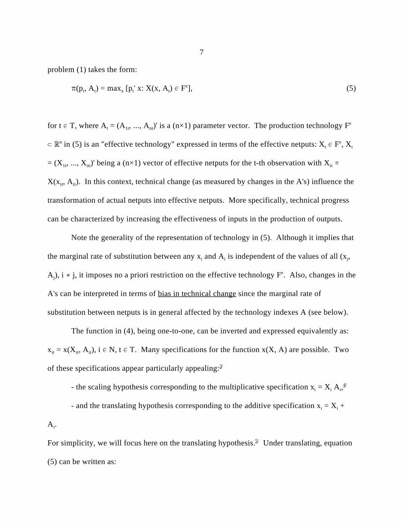
The function in (4), being one-to-one, can be inverted and expressed equivalently as:

x = x(X , A ), i N, t T. Many specifications for the function x(X, A) are possible. Twoit it it

of these specifications appear particularly appealing:3/

- the scaling hypothesis corresponding to the multiplicative specification x = X A , i i i4/

- and the translating hypothesis corresponding to the additive specification x = X +i i

A . i

For simplicity, we will focus here on the translating hypothesis. Under translating, equation5/

(5) can be written as:

8

(p , A ) = max [p ' (X+A ): X F ]t t X t te

= p 'A + max [p ' X: X F ], (6)t t X te

for t T. Equation (6) is a standard profit maximizing problem similar to (1), except that it

involves the effective netputs X. The associated Weak Axiom of Profit Maximization

(WAPM, corresponding to (2)) is:

p ' X p ' X , s, t T, (7)t t t s

or

p ' [x -A ] p ' [x -A ], s, t T. (7')t t t t s s

Next, consider some values for the A's that satisfy equation (7') for a given data set T. Using

these values, we can obtain the corresponding effective netputs: X = x - A . These effectivet t t

netputs necessarily satisfy the WAPM condition (7) for all s, t T. It is then clear from (6)

and (7) that all the results related to actual netputs x and presented in proposition 1 apply as

well to these effective netputs X. In particular, after substituting X for x, equation (3) gives a

representation of the underlying effective technology given by

F = {X: p ' X p ' X , t T; X 0 for i N ; X 0 for i N }. (8)T t t t i O i Ie

As we will see below, using equation (8) as a representation of the effective technology will

prove useful in the empirical evaluation of technical change.

Finally, under translating, note that any change in the technology parameters A across

observations has a simple interpretation in terms of the bias in technical change. First

9

consider the case of inputs, x 0 for i N . Given X = x - A , finding A A means thati I i i i it' it

technical change from t to t' is i -input using: ceteris paribus, a lower value of A implies thatthi

producing the same effective netputs X requires more of the i input (-x 0). Alternatively,thi

finding A A means that technical change from t to t' is i -input saving: ceteris paribus, ait' itth

higher value of A implies that producing the same effective netputs X can be produced withi

less of the i input (-x 0). Second, consider the case of outputs, x 0 for i N . Given Xthi i O i

= x - A , finding A A means that technical change from t to t' is i -output reducing:i i it' itth

ceteris paribus, a lower value of A implies that less of the i output can be produced with theith

same effective netputs X. Alternatively, finding A A means that technical change from tit' it

to t' is i -output augmenting: ceteris paribus, a higher value of A implies that more of the ith thi

output can be produced with the same effective netputs X. Finally, a technical change from

A to A that satisfies A = A can be interpreted as being neutral toward the i netput sincet t' it it'th

producing the effective netputs X can be done using the same quantity of the i netput x ,thi

ceteris paribus. This specification can thus provide a basis for analyzing technical change

bias (and the induced innovation hypothesis) on the input side as well as the output side. This

indicates that the nonparametric approach to production analysis can provide considerable

flexibility in the analysis of technology and technical change.

IV- Model Specification:

In this section, we develop a nonparametric method that can be used in the

investigation of the source and nature of technical change. While we have just argued that

technology indexes A that satisfy (7') can provide valuable information, it would be useful to

Ait it

m

j 0{[ ij (Pi,t j 1) ij]Rt j}, i N, t T,

10

(9)

obtain more specific insights as to the factors influencing technical progress. This can be

done by developing specific hypotheses about the determinants of the A's.

Much research has focused on the role of research in generating technical progress.

Investment in R&D is expected to stimulate the development of new technologies that can

improve productivity. However, the process of technical change takes time, suggesting the

existence of lag relationships between research and productivity. This indicates that the

technology indexes A can be modeled as a function of past R&D investments. Also, the

induced innovation hypothesis indicates that innovative activities tend to be guided by relative

resource scarcity. This suggests that the marginal impact of R&D depends on relative prices.

On that basis, we propose the following model specification for the A's:

where:

R is a (k×1) vector of R&D investments made at time t-j. In the analysis presentedt-j

below, we will distinguish between public and private R&D investments. This

corresponds to k = 2 and R = (Rpub, Rpri).

P is a relative price index for the i-th netput at time t-j.i,t-j

is an intercept reflecting the value taken by A in the absence of R&D investments.it it

m is the maximum number of lags between R&D investment and its impact on

productivity.

11

is a (1×k) parameter vector measuring the marginal effect of R on A whenij t-j it

relative prices are constant (corresponding to P = 1).i,t-j

is a (1×k) parameter vector measuring the interaction effect of P and R on A . ij i,t-j t-j it

Note that setting = 0 would imply that relative prices play no role in guiding the effects ofij

R&D. And assuming A / R > 0, the induced innovation hypothesis suggests that > 0. it t-j ij

To see that, note that an increase in the relative price P tends to increase the marginali,t-j

impact of R&D on A , thus increasing A . On the input side (x 0 for i N ), with X = x -it it i I i i

A , a higher A corresponds to biased technical change in the direction of decreasing the usei it

of the i input (-x 0). This is Hicks' induced innovation hypothesis: a rise (decline) in the ith thi

input cost tends to stimulate i input-saving (i input-using) technical change. On the outputth th

side (x 0 for i N ), with X = x - A , a rise in A corresponds to biased technical change ini O i i i it

the direction of increasing output x . This is the multi-output version of the inducedi

innovation hypothesis: a rise (decline) in the i output price increases (decreases) theth

profitability of the i output, which tends to stimulate innovations and generate i output-th th

augmenting (i output-reducing) technical change. Thus, throughout the rest of the paper, weth

will interpret > 0 in (9) as being consistent with the induced innovation hypothesis. ij

Alternatively, finding 0 would be inconsistent with this hypothesis. Note that this is aij

dynamic version of the induced innovation hypothesis since it considers the guiding role of

prices in the lagged effects of R&D investments. It is fairly general since it allows toij

change magnitude (and possibly sign) with the lags j. In other words, for each netput i, this

Ait

r

j 1Ai,t j

r, i NO.

12

(10a)

specification allows the presence and strength of the induced innovation hypothesis to vary

through an innovation cycle.

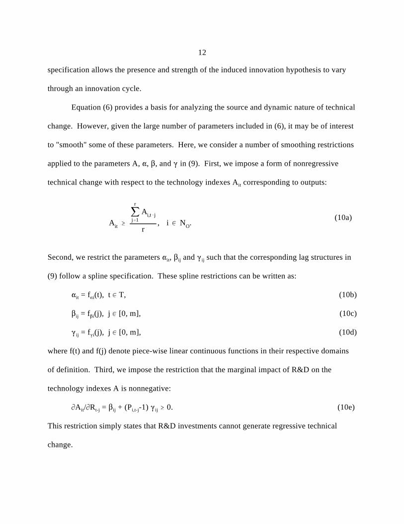
Equation (6) provides a basis for analyzing the source and dynamic nature of technical

change. However, given the large number of parameters included in (6), it may be of interest

to "smooth" some of these parameters. Here, we consider a number of smoothing restrictions

applied to the parameters A, , , and in (9). First, we impose a form of nonregressive

technical change with respect to the technology indexes A corresponding to outputs:it

Second, we restrict the parameters , and such that the corresponding lag structures init ij ij

(9) follow a spline specification. These spline restrictions can be written as:

= f (t), t T, (10b)it i

= f (j), j [0, m], (10c)ij i

= f (j), j [0, m], (10d)ij i

where f(t) and f(j) denote piece-wise linear continuous functions in their respective domains

of definition. Third, we impose the restriction that the marginal impact of R&D on the

technology indexes A is nonnegative:

A / R = + (P -1) 0. (10e) it t-j ij i,t-j ij

This restriction simply states that R&D investments cannot generate regressive technical

change.

13

Finally, while equation (9) can provide useful insights in the process of technical

change, it does not make explicit the relationship between R&D and productivity. To

examine this linkage, it is necessary to estimate a productivity index that is consistent with

equation (9). Assume that all observations are technically efficient, i.e., that each observation

is on the boundary of the feasible set representing the technology available when each

observation is made. Following Caves et al. (1982), consider the input-based productivity

index: Q(x) = min {k: (x , -k x ) F, k }. For a given x = (x , x ), Q is the smallestk O I O I+

rescaling of all inputs x that remains feasible in the production of outputs x underI O

technology F. An index Q > 1 (< 1) means that the netput vector x = (x , x ) uses a betterO I

technology (an inferior technology) compared to the technology represented by F. In this

context, if Q < 1 (Q > 1), then (1 - Q) can be interpreted as the percentage cost reduction (cost

increase) that is achieved by shifting from the current technology to technology F. Using the

effective technology F in (8), we can then define the following productivity index associatedTe

with the observation x:

Q(x, A) = min {k: p ' x + p ' (k x ) p X ; X = x - A ; t T; k }, (11)k Ot O It I t t t t t+

The productivity index Q(x, A) in (11) provides a simple radial measure of the distance

between observation x and the technology F . But F depends on the technology indexes A,T Te e

which in turn depend on R&D investments through equation (9). It follows that the index

Q(x,A) in (11), along with equation (9), can provide a basis for measuring the dynamic impact

of R&D investments on productivity. The usefulness of these results is illustrated next in the

context of an application to U.S. agriculture.

14

V- An Application to U.S. Agriculture:

We consider the analysis of technical change in U.S. agriculture between 1951 and

1983. The data used in the analysis consists of annual observations on quantity and price

indexes for six categories of outputs and ten categories of inputs from 1920 to 1983. The

price and quantity indexes from 1950 to 1983 are obtained from Capalbo and Vo. For the

period 1920-1950, the price and quantity indexes are calculated from U.S. Department of

Agriculture published data, following the Capalbo-Vo method as closely as possible. All6/

price indexes are implicit price indexes defined such that price times quantity equals

expenditure. The output categories are: 1/ small grains; 2/ coarse grains; 3/ other field crops;

4/ fruits; 5/ vegetables; and 6/ animal products. The input categories include: 1/ family labor;

2/ hired labor; 3/ land; 4/ structures; 5/ other capital; 6/ energy; 7/ fertilizer; 8/ pesticides; 9/

feed and seed; and 10/ other inputs. The data provide a basis for evaluating technical change

in U.S. agriculture over the last few decades. We also analyze the effects of both public and

private agricultural R&D on technical progress. The agricultural R&D data (both private and

public) are taken from Huffman and Evenson.

Based on the discussion presented in previous sections, we consider the following

optimization problem:

min [ { w + (w +w )}: equations (7'), (9) and (10); A, , , i N t T 1 it j 2 ij 3 ij2 2 2

x -A 0, i N ; x -A 0, i N ; t T], (12)it it O it it I

where (w , w , w ) are positive weights. Note that the solution to (12) for the A's is1 2 37/

necessarily consistent with the WAPM conditions (7) or (7'). Obtaining this solution is

15

straightforward since (12) can be formulated as a standard optimization problem. Using the

solution from (12) for the A's, we can obtain the corresponding effective netputs: X = x - A . t t t

These effective netputs necessarily satisfy the WAPM condition (7) for all s, t T. Equation

(8) gives a representation of the underlying effective technology F . Since equation (12)Te

searches for the smallest absolute values of the 's, 's and 's (and thus the A's) that are

consistent with profit maximization, F in (8) can be interpreted as the technology that is "asTe

close to the data as possible" while satisfying WAPM in (6) for all data points. Finally, the

solution to equation (12) provides estimates of the parameters , and which characterize

the dynamic effects of R&D and the associated innovation process.

In the empirical implementation of (12) in the context of U.S. agriculture, the

following assumptions are made. The maximum number of lags m in equation (9) is set equal

to 28 years. This is consistent with the empirical evidence presented by Pardey and Craig

(1989), who identify a maximum lag between agricultural R&D and productivity of about 30

years. Thus the values of , , and in (9) need to be estimated for i N and 0 j 28.it ij ij

The relative price P in (9) is calculated as the ratio of the price index for the i inputith

(output), divided by the Tornqvist aggregate price index for all inputs (all outputs). The8/

value of r in (10a) is set equal to 5 years, implying nonregressive technical change of the A 'sit

with respect to their previous five-year moving averages. The restrictions in (10b) are

imposed only for inputs, i.e., for i N . The spline restrictions for (10b) involve continuousI9/

linear segments for the periods 1951-61, 1961-72 and 1972-82. And the spline restrictions

(10c) and (10d) are imposed using four continuous linear segments: 0-7 years, 7-14 years, 14-

21 years, and 21-28 years. End-point restrictions (at 0 years and 28 years) are imposed,

16

forcing the functions to be equal to zero at these points. Finally, while the 's and the 'sij ij

are allowed to be non-zero for public R&D for 0 < j < 28, these parameters are further

restricted for private R&D. This is motivated by current U.S. patent laws, which grant private

inventors exclusive rights to their inventions for a period of 17 years. During this period,

patents are legally protected from infringement by competitors. However, there is little

incentive for private investment in research with payoffs much beyond the enforcement

period. Therefore, the 's and the 's for private R&D are restricted to be equal to zero forij ij

21 j 28.

The only issue left then is the choice of the weights (w , w , w ) in the objective1 2 3

function (12). In the empirical results presented below, we chose these weights such that, at

1967 values, the relative marginal impacts of , and in problem (12) are the same. This

can be interpreted to mean that, in our approach, we assume no a priori bias about the relative

importance of the three terms in equation (9).

Selected results on the estimates of the A's obtained from the solution to (12) are

presented in Figure 1. The A's associated with outputs tend to increase over time. This is

consistent with technical progress. Selected estimates of the 's and 's are presented in

Figures 2a, 2b and 2c for both public and private R&D.

On the input side (i N ), the results presented in Figures 2a and 2b are somewhatI

mixed concerning the induced innovation hypothesis. The results for labor are inconsistent

with the hypothesis (see Figure 2a). The estimates of the 's for land and structure are either

zero or close to zero, suggesting that relative prices do not play a major role in influencing the

bias of technical change for these inputs. In contrast, the estimates of the 's for energy,

17

fertilizer, and pesticides provide rather strong evidence in favor of the induced innovation

hypothesis ( > 0) (see Figure 2b). These findings are consistent with previous researchij

(e.g., Binswanger; Hayami and Ruttan). Thus, in general, our findings provide some support

for the induced innovation hypothesis with respect to inputs that are more actively traded

(e.g., energy, fertilizer, pesticides). However, we do not find any evidence in favor of

induced innovation for inputs that are less actively traded (e.g., land, farm labor). This

suggests that the lack of active markets may undermine the economic intuition that motivates

the induced innovation hypothesis. In such situations, it may well be that nonmarket forces

play a more significant role in determining the bias in technical change.

On the output side (i N ), the results in Figure 2c are consistent with the inducedO

innovation hypothesis ( > 0). This indicates that changes in relative output prices tend toij

guide the innovation process and generate biased technical change in favor (against) outputs

that are becoming more (less) profitable. However, some significant differences appear to

exist between private and public R&D effects. In general, the values of the 's and 's for

private R&D are positive for lags between 0 and 15 years, but zero for lags beyond 15 years.

In contrast, the values of the 's and 's for public R&D are either small or zero in the short

term, but tend to become positive and larger in the longer term (lags between 15 and 28

years). This suggests that public R&D (private R&D) has a more important effect on

productivity in the longer-term (shorter-term). This result will be further illustrated below.

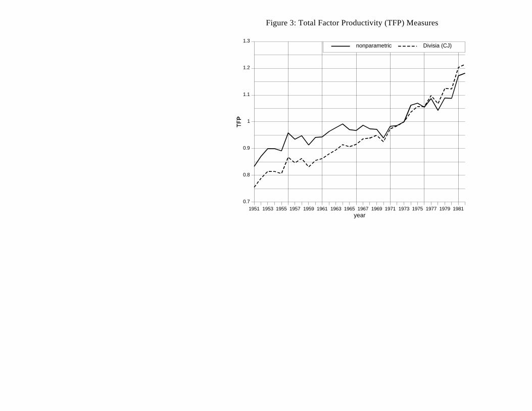
Given the solution obtained in (12), the importance of technical change and

productivity gains in U.S. agriculture was evaluated using equation (11). The nonparametric

productivity index Q obtained from (11) is presented in Figure 3, along with the Christensen-

18

Jorgenson Divisia productivity index commonly used in the literature (e.g., Ball, 1985).

These indexes indicate that the U.S. agricultural sector has been the subject of significant

technical progress over the last few decades. This is consistent with previous research done

on this topic (e.g., Jorgenson and Gollop, 1992; Chavas and Cox, 1992). In general, the

Christensen-Jorgenson Divisia productivity index tends to rise faster than our nonparametric

productivity index (see Figure 3). This difference suggests that our nonparametric

representation of the effective technology does not approximate the parametric restrictions

needed to justify the Christensen-Jorgenson productivity index.10/

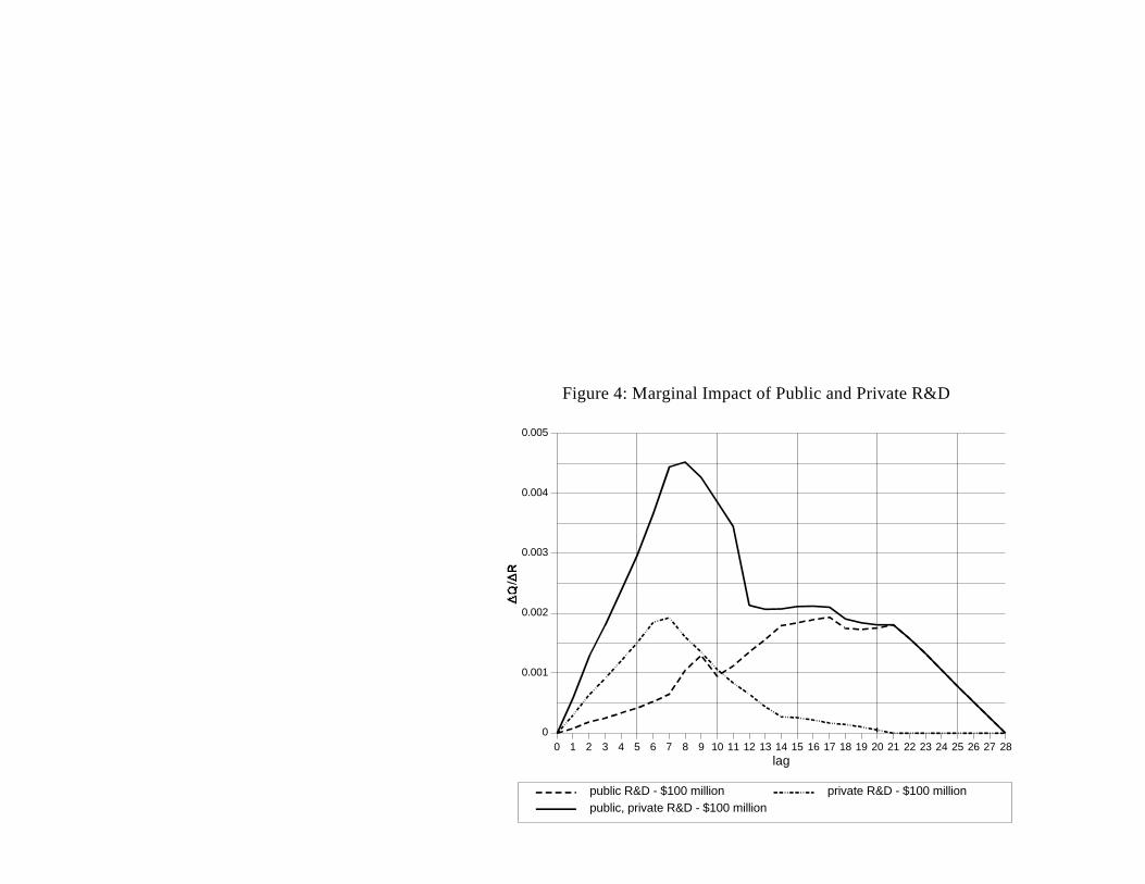
The marginal impact of R&D on productivity was also evaluated numerically by

solving equation (11) for different levels of both public and private R&D. The results are

presented in Figure 4. They indicate that both public and private R&D have a large and

positive effect on productivity. Figure 4 also shows important differences in the dynamic

impacts of private versus public R&D. Private R&D has a strong short-term effect on

productivity (after 5 to 10 years) and basically little longer-term effect. This is consistent with

current patent rights applicable to private institutions, which grant inventors exclusive rights

to their invention for a period of 17 years (thus providing little incentive for private

investment in research with longer-term payoffs). In contrast, public R&D has a small short-

term impact on productivity, but a larger positive impact in the longer-term (after 15 to 22

years).

Our results have interesting implications concerning the current shift in R&D funding

from public to private. Figure 4 shows that private R&D generates larger benefits in the

short-run compared to public R&D. It also shows that public research has a strong but

19

longer-term impact on productivity. This suggests that a substitution of current R&D funding

from public to private would increase productivity in the short-term (after 0-10 years), but

would tend to reduce the rate of technical progress in the longer-term (beyond 15 years).

Finally, the marginal impacts of R&D on productivity presented in Figure 4 can be

used to estimate the internal rate of return to public and private research. Interpreting the

productivity index as a measure of the cost savings generated by technical progress, we

calculate the benefits of an additional $100 million of R&D investment in terms of the

associated reduction in production costs. We then evaluate the associated internal rate of

return for public as well as private research. The estimated rates of return are 0.27 for public

R&D, and 0.46 for private R&D. These results are fairly similar to those found in previous

studies (e.g., Griliches, 1958; Evenson, 1967; Bredhal and Peterson, 1976; Knutson and

Tweeten, 1979; Chavas and Cox, 1992). Thus, these findings are consistent with previous

evidence: in general, the internal rates of return to private as well as public research are fairly

high.

VI- Conclusion:

This paper presents a nonparametric methodology to investigate the nature of technical

change, with a special focus on the effects of both private and public R&D on productivity.

The method is illustrated in an application to U.S. agriculture. The approach is fairly flexible:

it does not require explicit assumptions about the form of the underlying production

technology; it allows for biased technical change using disaggregate inputs and outputs (ten

inputs and six outputs in our case); and it allows for refined lag specifications between R&D,

20

relative prices, and technology indexes. The application to U.S. agriculture provides useful

information on the source and nature of technical change.

The dynamic effects of private and public R&D on technical change differ. The

effects of private research are larger in the short-term (5 to 15 years) but small in the longer-

term. In contrast, the returns from public research are small in the short-term, but larger in the

longer-term (15-25 years). However, the internal rates of return from both private and public

R&D are found to be fairly large. This provides additional evidence of the high productivity

of both private and public research in the U.S. agricultural sector. The results also give some

empirical support in favor of the induced innovation hypothesis for the netputs that are

actively traded: for these netputs, market signals tend to guide the direction of the bias in

technical change. However, our results do not support the induced innovation hypothesis for

the inputs that are less actively traded: land and farm labor. This suggests that, for these

inputs, non-market forces may play a more significant role in guiding the innovation process.

The empirical results presented here illustrate the usefulness of the nonparametric

approach in the analysis of production and technical change. The nonparametric method,

however, has its limitations. First, it remains subject to measurement problems typically

involved in the investigation of technical change. Second, its main limitation may be the

absence of hypothesis testing, as the method is not statistically based. Nevertheless, the

empirical results presented here appear reasonable and often comparable with those obtained

from previous research. As such, the proposed methodology appears to be a useful

complement to more traditional parametric methods in the economic analysis of production

issues and technical change.

Figure 1: Technology Indexes for Selected Netputs

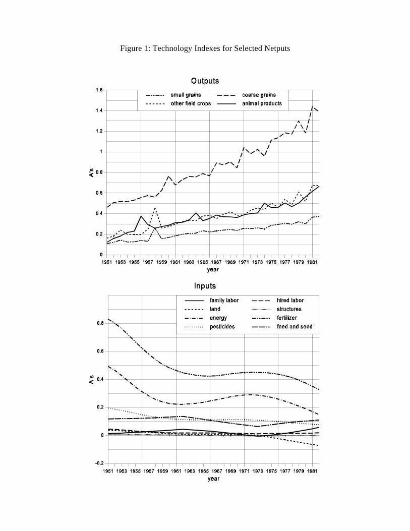
Figure 2a: Selected Estimates of the 's and 's

Figure 2b: Selected Estimates of the 's and 's (continued)

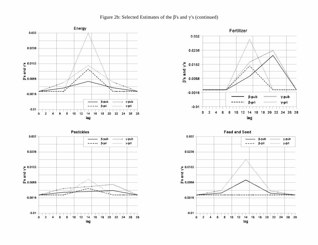
Figure 2c: Selected Estimates of the 's and 's (continued)

year1951 1953 1955 1957 1959 1961 1963 1965 1967 1969 1971 1973 1975 1977 1979 1981

0.7

0.8

0.9

1

1.1

1.2

1.3nonparametric Divisia (CJ)

Figure 3: Total Factor Productivity (TFP) Measures

public R&D - $100 million private R&D - $100 millionpublic, private R&D - $100 million

lag0 1 2 3 4 5 6 7 8 9 10 11 12 13 14 15 16 17 18 19 20 21 22 23 24 25 26 27 28

0

0.001

0.002

0.003

0.004

0.005

Figure 4: Marginal Impact of Public and Private R&D

REFERENCES

Afriat, S.N. "Efficiency Estimation of Production Functions." International Economic Review 13(October 1972):568-598.

Ball, V.E. "Output, Input, and Productivity Measurement in U.S. Agriculture, 1948-79" American Journal of Agricultural Economics

67(1985):475-486.

Binswanger, H.P. "The Measurement of Technical Change Biases with Many Factors of Production" American Economic Review

64(1974):964-976.

Binswanger, H.P. and V.W. Ruttan Induced Innovation: Technology, Institutions and Development Johns Hopkins University Press, Baltimore,

1978.

Banker, R.D. and A. Maindiratta "Nonparametric Analysis of Technical and Allocative Efficiencies in Production" Econometrica 56(November

1988):1315-1332.

Bredahl, M. and W. Peterson "The Productivity and Allocation of Research: U.S. Agricultural Experiment Stations" American Journal of

Agricultural Economics 58(1976):684-692.

Capalbo, S.M. and T.V. Vo "A Review of the Evidence on Agricultural Productivity and Aggregate Technology" in Agricultural Productivity:

Measurement and Explanation S.M. Capalbo and J.M. Antle, editors, Resources for the Future, Inc., Washington D.C., 1988.

Caves, D.W., L.R. Christensen, and W.E. Diewert "The Economic Theory of Index Number and the Measurement of Input, Output, and

Productivity" Econometrica 50(1982):1393-1414.

Chavas, J.P. and T.L. Cox "A Nonparametric Analysis of Productivity: The Case of U.S. and Japanese Manufacturing" American Economic

Review 80(June 1990):450-464.

Chavas, J.P. and T.L. Cox "A Nonparametric Analysis of the Influence of Research on Agricultural Productivity" American Journal of

Agricultural Economics 74(1992):583-591.

Christensen, L.A. and D. Jorgenson "U.S. Real Product and Real Factor Input, 1929-1967" Review of Income and Wealth 16(1970):19-50.

Evenson, R.E. "The Contribution of Agricultural Research to Production" Journal of Farm Economics 49(1967):1415-1425.

Griliches, Z. "Hybrid Corn: An Exploration of the Economics of Technical Change" Econometrica 25(1957):501-522.

Hanoch, G. and M. Rothschild "Testing the Assumptions of Production Theory: A Nonparametric Approach" Journal of Political Economy

80(1972):256-275.

Hayami, Y. and V.W. Ruttan Agricultural Development: An International Perspective Johns Hopkins University Press, Baltimore, 1985.

Hicks, J.R. The Theory of Wages Macmillan and Co. Ltd., London, 1932.

Huffman, W.E. and R.E. Evenson Science for Agriculture: A Long Term Perspective Iowa State University Press, Ames, 1993.

Jorgenson, D.W. and F.M. Gollop "Productivity Growth in U.S. Agriculture: A Postwar Perspective" American Journal of Agricultural

Economics 74(1992):745-750.

Knutson, M. and L.G. Tweeten "Toward an Optimal Rate of Growth in Agricultural Production Research and Extension" American Journal of

Agricultural Economics 61(1979):70-76.

Olmstead, A.L. and P. Rhodes "Induced Innovation in American Agriculture: A Reconsideration" Journal of Political Economy 101(1993):100-

118.

Pardey, P.G. and B. Craig "Causal Relationships between Public Sector Agricultural Research Expenditures and Output" American Journal of

Agricultural Economics 71(1989):9-19.

Pollak, R.A. and T.J. Wales "Demographic Variables in Demand Analysis" Econometrica 49(1981):1533-1551.

Solow, R.M. "Technical Change and the Aggregate Production Function" Review of Economics and Statistics 39(1957):312-320.

Solow, R.M. "Some Recent Developments in the Theory of Production" in The Theory and Empirical Analysis of Production Murray Brown,

ed., National Bureau of Economic Research, New York, 1967.

Varian, H. "The Nonparametric Approach to Production Analysis" Econometrica 52(May 1984):579-597.

1. The convexity of F means that, for any x F and x F, then [ x + (1- ) x ] F for any , 0 < < 1. This corresponds toa b a b

the standard assumption of "non-increasing marginal productivity" commonly made in economics.

2. Negative monotonicity of F means that for any x F and x x , then x F. This is sometimes called the "free disposal"a b a b

assumption.

3. For example, see Pollak and Wales for the use of scaling and translating hypotheses in the context of consumer demand.

4. Note that the use of scaling in the analysis of technical change has been proposed and discussed by Solow (1967).

5. In the context of scaling, equation (5) becomes(p , A ) = max [p ' (X A ): X F ]t t X t t

e

for t T. The associated Axiom of Profit Maximization is:p ' x p ' [y A /A ], s, t T.t t t s s t

Note that, in contrast with (7'), the above expression is nonlinear in A. This nonlinearity makes the scaling hypothesis moredifficult than the translating hypothesis to use empirically.

6. Quantity indexes calculated from disaggregate information are obtained using Tornqvist indexes. Service prices for all capitalassets are calculated according to the method outlined by Christensen and Jorgenson. Pre-1940 data for land and structures areestimated from Tostlebe. Note that, for some of the pre-1950 data, it was not possible to follow exactly the Capalbo-Vo method. For example, in the absence of a reliable source of information, we assumed the same unit price before 1950 for family labor andhired labor. Also, we did not quality-adjust the pre-1950 labor data.

7. The choice of these weights is discussed below.

8. The relative price indexes are all normalized to be equal to 1 in 1967. As a result, (P -1) in equation (9) can be interpreted asi

the percentage change in the relative price of the i netput compared to the 1967 situation.th

9. As a result, the are "unsmoothed" for outputs, i.e., for i N . This was done to account for possible weather shocks that canit O

affect outputs from one year to the next.

10. As shown by Caves et al. (1992), the Christensen-Jorgenson productivity index is appropriate if the frontier technology canbe represented by a linear homogenous translog function with constant second-order coefficients. The difference between the twoproductivity indexes reported in Figure 3 can thus be interpreted to mean that our nonparametric representation of the technologydoes not approximate these parametric restrictions.

Footnotes