University of Warwick institutional repository: · Tahani Mohammad Bawazeer A thesis submitted for...
179
University of Warwick institutional repository: http://go.warwick.ac.uk/wrap A Thesis Submitted for the Degree of PhD at the University of Warwick http://go.warwick.ac.uk/wrap/56925 This thesis is made available online and is protected by original copyright. Please scroll down to view the document itself. Please refer to the repository record for this item for information to help you to cite it. Our policy information is available from the repository home page.
Transcript of University of Warwick institutional repository: · Tahani Mohammad Bawazeer A thesis submitted for...

University of Warwick institutional repository: http://go.warwick.ac.uk/wrap
A Thesis Submitted for the Degree of PhD at the University of Warwick
http://go.warwick.ac.uk/wrap/56925
This thesis is made available online and is protected by original copyright.
Please scroll down to view the document itself.
Please refer to the repository record for this item for information to help you to cite it. Our policy information is available from the repository home page.

Developments of New Techniques
for Studies of Coupled Diffusional and Interfacial
Physicochemical Processes
By
Tahani Mohammad Bawazeer
A thesis submitted for the degree of
Doctor of Philosophy
Department of Chemistry
United Kingdom
December 2012

For
my parents…
my husband…
and my Children…
I would never have
reached this point without you,
and I will never be able to thank you enough
Table of Contents
ii
Table of Contents ii
List of Illustrations v
List of Tables xii
List of Abbreviations xiii
List of Symbols xv
Acknowledgment xvii
Declaration xviii
Abstract xix
Chapter 1 Introduction 1
1.1 Fluorescence Confocal Laser Scanning Microscopy (CLSM) 1
1.1.1 Literature Survey 1
1.1.2 CLSM Principle 4
1.1.3 Fluorescence 6
1.1.3.1 Fluorescein 8
1.2 Electrochemistry and Microelectrodes 11
1.2.1 Introduction to electrochemistry 11
1.2.2 Dynamic electrochemistry 12
1.2.3. Mass transport 15
1.2.3.1 Diffusion 16
1.2.3.2 Convection 18
1.2.3.3 Migration 18
1.2.4 Ultramicroelectrodes (UME) 19
1.2.5 Linear Sweep Voltammetry and Cyclic Voltammetry 22
1.2.6 Scanning electrochemical microscopy (SECM) 25
1.2.6.1 Negative Feedback 26
1.2.6.2 Positive Feedback 28
1.4 Finite Element Modelling (FEM) 28
1.5 Aims of the Thesis 31
1.6 References 33
Chapter 2 Experimental Methods 37
2.1 Sample Preparation 37
Table of Contents
iii
2.2 Device Microfabrication and Characterisation 39
2.2.1 Pt Ultramicroelectrode (UME) Fabrication and Characterisation 39
2.2.2 Optical Transparent Single-Walled Carbone Nanotubes
Ultramicroelectrodes (OT-SWNTs-UMEs) mat Fabrication
42
2.3 CLSM Experiments 47
2.3.1 Visualisation of Electrochemical Processes at OT-SWNTs-UMEs 48
2.3.2 Visualization of Proton Diffusion at active and Modified Surfaces 51
2.4 Additional Instrumentation 58
2.4.1 Inductively Coupled Plasma Mass Spectroscopy (ICP-MS) 58
2.4.2 Fluoride Ion Selective Electrode (FISE) Studies 59
2.5 Finite Element Modelling 59
2.6 Solution Preparation 59
2.7 References 61
Chapter 3 Visualisation of Electrochemical Processes at Optically
Transparent Single-Walled Carbon Nanotubes
Ultramicroelectrodes (OT-SWNTs-UMEs)
62
3.1 Overview 62
3.2 Introduction to Carbone Nanotube 69
3.2.1 Characterisation of SWNTs ultrathin films 73
3.2.2 Characterisation of SWNTs disc OT-UMEs 74
3.3 Visualisation of the ORR at SWNTs disc OT- UME 76
3.3.1 Dynamic Visualisation of Ru(bpy)32+
concentration during CV
measurements at SWNTs disc OT- UME.
79
3.3.2 Three dimensional concentration profiles of Ru(bpy)32+
at the
steady-state current.
81
3.4 Conclusion 85
3.5 References 87
Chapter 4 Transient Interfacial Kinetics, from Confocal Fluorescence
Visualisation: Application to Proton Attack the Treated
Enamel Substrate
90
4.1 Overview 90
Table of Contents
iv
4.1.1 Enamel Structure 92
4.1.2 Enamel Dissolution 93
4.1.3 Enamel Dissolution Inhibitors 94
4.2 Proton Distribution at Disc UME 95
4.3 CLSM Visualisation of Proton Flux during Enamel Dissolution 96
4.3.1 Experimental Results and Analysis 97
4.4 Finite Element Model 103
4.4.1 Diffusion Coefficients 107
4.4.2 Insights from Simulations 109
4.5 Amount of Zinc and Fluoride Uptake on Treated Enamel 113
4.6 Conclusions 114
4.7 References 116
Chapter 5 Combined Confocal Laser Scanning Microscopy -
Electrochemical Techniques for the Investigation of Lateral
Diffusion of Protons at Surfaces
119
5.1 Biological Membranes 119
5.2 Supported Lipid Bilayer (SLB) Synthesis and Characterisation 123
5.3 Modification of Surfaces by Ultrathin Films 126
5.4 Proton Lateral Diffusion 128
5.5 Result and Discussion 132
5.5.1 Characterisation of SLB-Modified Surfaces by AFM 132
5.5.2 Measurement of proton diffusion at modified surfaces 134
5.6 Conclusion 145
5.7 References 147
Chapter 6 Conclusion 151
Appendix 155

List of Illustrations
v
List of Illustrations
Chapter 1 Introduction 1
Figure 1.1 (a) Full-field illumination (b) Single point illumination 4
Figure 1.2 Schematic diagram of a confocal microscope 5
Figure 1.3 Schematic of 3D z-stack imaging in CLSM 6
Figure 1.4 A Jablonski diagram showing the origin of fluorescence, with the
photoexitation of an electron from (1) to (2) and emission light
when the electron moves from (3) to (1)
7
Figure 1.5 Definition of Stokes shift 8
Figure 1.6 Illustration of pH vs. intensity of fluorescence after fluorescein
excitation at 488 nm and detection at 530 nm
9
Figure 1.7 Molecular structures of neutral fluorescein and its anions 10
Figure 1.8 A diagrammatic representation of the electrical double layer
where the red cations are solvated with small blue circles
representing water molecules, and large green anions are
specifically adsorbed onto the electrode surface
12
Figure 1.9 The effect of the applied potential on the Fermi level 13
Figure 1.10 A schematic representation of a typical electrode reaction 14
Figure 1.11 Different geometries of electrodes and their diffusion fields: (a)
Disk electrode (b) Cylinder electrode and (c) Ring electrode
Reproduced from reference
20
Figure 1.12 (a) Schematic of planar diffusion profile exhibited by a
macroelectrode and (b) the hemispherical diffusion at disc UME
21
Figure 1.13 Showing the RG of an UME where rs is the radius of the whole
UME and a is the radius of the metal wire
22
Figure 1.14 Typical CV responses for (a) a macroelectrode and (b) an
ultramicroelectrode
23
Figure 1.15 (a) Schematic of negative feedback, for an UME near an
insulating substrate and (b) Theoretical approach curve for a 25
µm diameter UME with an RG of 10, depicting negative feedback
27
Figure 1.16 (a) Schematic of positive feedback near a conducting substrate (b)
Theoretical approach curve for a 25 µm diameter UME displaying
positive feedback
28

List of Illustrations
vi
Figure 1.17 (a) An example of a simple triangular mesh used for FEM and
(b)the same domain where the mesh is finer at two edges
30
Chapter 2 Experimental Methods 37
Figure 2.1 Conventional light microscope image of the tip of a 25 μm
diameter platinum disc UME (a) from the side (b) the electrode
surface
40
Figure 2.2 Cyclic voltammogram for the oxidation of 1 mM FcTMA at a 25-
μm diameter Pt UME. The scan rate was 10 mV s-1
41
Figure 2.3 SECM experimental approach curve (red line) and the theory
(blue line) towards inert glass substrate performed in 0.1 M KNO3
42
Figure 2.4 Schematic illustration the procedure for growing carbon nanotube
ultrathin mats using catalysed chemical vapour deposition
technique
43
Figure 2.5 (a) Schematic of the procedure used for fabricating SWNTs
network disk UMEs, (bi) Geometry of the shadow mask used for
microfabrication of Cr/Au bands for disk UME experiments, (bii)
Photographs of SWNTs devices used in electrochemical
experiments
45
Figure 2.6 Micro-Raman spectrum of SWNTs ultrathin mats grown on single
crystal quartz
47
Figure 2.7 Schematic representation of the experimental setup used for
visualising OT-SWNTs-UMEs
49
Figure 2.8 Schematic diagram of the clamp system developed for use with
the confocal microscope
51
Figure 2.9 (a) Rise time for a current of 20 nA using homemade galvanostat
and (b) corresponding change of the potectial applied to the UME
working electrode
52
Figure 2.10 Describes the CLSM-SECM set-up where: (a) is a schematic
detailing the components seen in (b); (b) is a photograph showing
the UME and enamel sample inserted in the cell and immersed in
solution
53
List of Illustrations
vii
Figure 2.11 Experimental set up for SECM tip positioning and CLSM
experiments
55
Figure 2.12 Schematic (not to scale) of experimental arrangement for studies
of proton diffusion at a SLB
57
Figure 2.13 Schematic of experimental arrangement for studies of proton
diffusion in a thin layer
58
Chapter 3 Visualisation of Electrochemical Processes at Optically
Transparent Single-Walled Carbon Nanotubes
Ultramicroelectrodes (OT-SWNTs-UMEs)
62
Figure 3.1 a) AFM (3 nm × 3 nm) AFM images (full height scale=5 nm) of a
SiO2 surface after cCVD growth of SWNTs. b) associated FE-
SEM image of a SWNT network. The scale bar represents 5 μm.
Taken from reference
71
Figure 3.2 (a) 1 µm × 1 µm tapping mode AFM height images of SWNT
networks and ultrathin mats grown on single crystal ST-cut quartz
substrate, using Co as the catalyst, sputter-deposited on the
substrate 20 s prior to growth. (b) Micro-Raman spectrum of
SWNT ultrathin mats grown on single crystal quartz
74
Figure 3.3 UV-Vis spectra of: blank ST-cut quartz; SWNT mat grown on ST-
cut quartz substrate; and ST-cut quartz coated with S1818 positive
photoresist
75
Figure 3.4 (a) Brightfield mode (b) and fluorescence mode images of an
optically transparent carbon nanotube ultramicroelectrode
(zoomed out and zoomed in). The images were recorded in the x-y
plane parallel to the electrode
76
Figure 3.5 CV of ORR and simultaneous change of solution light intensity as
a function of potential, at a SWNT disc OT-UME (scan rate 10
mVs-1
) for 0.1 M NaCl aqueous solution with 8 µM fluorescein
and an initial pH 5. The arrows indicate the initial scan direction.
The intensity values were collected from the middle of the UME
surface, from a 35 µm diameters region of interest (ROI). The
fluorescence mode insets illustrate the development of pH
77
List of Illustrations
viii
gradients as a function of potential. The scale bars are 250 µm
Figure 3.6 (a) Fluorescence intensity at a potential of -1.0 V in 0.1 M NaCl
solution with 8 µM fluorescein in the xy, xz and yz planes. The
scale bar in the xy image is 250 µm. The red and white lines in xz
and yz cross sections indicate the photoresist and OT UME
surface. (b) A graph of intensity below (B) and above (A) the OT-
UME plane in 35 µm diameter ROI. The dashed line indicates the
electrode surface
78
Figure 3.7 (a) CV (red) and simultaneous change of the fluorescence
intensity (black: scan rate 5 mV/s) for the oxidation of 10 mM
Ru(bpy)32+
in aqueous solution in 0.1 M NaCl. The arrows
indicate the forward scan direction. The intensity values were
collected from the 35 mm diameter region of interest at the centre
of the UME. Intensity values and current values were normalised
by the initial intensity value at time = 0 s (It=0) and the steady-
state limiting current value (ilim), respectively. The insets show
fluorescence profiles near the OT-CNT-UME surface during
Ru(bpy)32+
oxidation. The scale bars are 25 mm. (b) Relationship
between normalised current and fluorescence intensity change for
forward andreverse scan directions in the range of quartile
potentials of the voltammetric signature
80
Figure 3.8 The change of solution intensity over time during stepping up the
potential from 0 V to the potential of the mass transport limiting
current (1.2 V), determined from the CV for 10 mM Ru(bpy)32+
aqueous solution in 0.1 M NaCl. The inlets indicate the formation
of the diffusion zone at the UME surface. The scale bar is 25 µm
82
Figure 3.9 Cross sectional light intensity change below and above the UME
surface before (left) and after (right) the potential step for the 1
mM (a), 5 mM (c), and 10 mM (e) Ru(bpy)32+
in 0.1 M NaCl (e).
All images were collected with the z-volume 150 µm (vertical
white dashed line) and the z-step 2 µm. Z-stack before the
potential step and during the steady state for the 1 mM (b), 5 mM
(d), and 10 mM (f) Ru(bpy)32+
in 0.1 M NaCl. The scale bars in (a,
84
List of Illustrations
ix
c) and (e) are 25 µm. Dark blue arrows indicate the -position of
the electrode surface in both scans. The light intensity values were
normalised taking into account the intensity signal from the 35 µm
diameter region of interest only
Chapter 4 Transient Interfacial Kinetics, from Confocal Fluorescence
Visualisation: Application to Proton Attack the Treated
Enamel Substrate
90
Figure 4.1 A cross sectional schematic of the structure of a tooth; (a)
represents the dental hard tissue enamel, (b) represents the dental
soft tissue dentine, (c) is the pulp containing the nerves, (d) is the
gum surrounding the tooth and (e) is the bone from which teeth
grow
92
Figure 4.2 CLSM image of water oxidation in 8 μM fluorescein solution with
0.1 M potassium nitrate at a 25 μm diameter Pt disc electrode with
applied currents of 10 nA (a), 50 nA (b) and 100 nA (c) at a bulk
solution pH of 7.5. The images were recorded in the x-y plane
parallel to the electrode.
96
Figure 4.3 Overlay of a brightfield with fluorescence modes (a) and
fluorescence mode images (b) of a UME close to enamel with a
tip-substrate separation of 20 µm, in 8 μM fluorescein solution
with 0.1 M potassium nitrate
97
Figure 4.4 Shows a series of images captured from the CLSM at times of 0
sec, when no current has passed, 1.22 seconds, 1.64 seconds, 2.89
seconds and 4.57 seconds (a) The proton distribution next to glass
substrate, (b) The proton dispersion near to an enamel substrate.
The yellow scale bar represents 75 m
98
Figure 4.5 Typical sigmoid fit to the right hand side of the fluorescence
intensity for water oxidation in 8 µl fluorescein aqueous solution
in (0.1 M NaCl). The intensity values were collected from the area
between the electrode and the surface of interest after the
application of the current
99
Figure 4.6 The impact upon the shape of the pH profiles next to glass and 100

List of Illustrations
x
enamel surfaces
Figure 4.7 Radial distance-time profile of the distance dependence of the pH
6.1 front in a thin layer of aqueous solution following the
oxidation of water at a 25 μm diameter Pt UME, positioned 20 μm
away from untreated enamel (black squares, black line), fluoride-
treated enamel (red circles, red line) and zinc-treated enamel (blue
triangles, blue line). Current applied: Current applied: (a) 20 nA ,
(b) 15 nA and (c) 10 nA
100
Figure 4.8 Simulation domain for the axisymmetric cylindrical geometry
used to model the formation of etch pits in dental enamel
104
Figure 4.9 Radial distance-time profile of the distance dependence of the pH
6.1 front in a thin layer of aqueous solution following the
oxidation of water at a 25 μm diameter Pt UME, matched to their
respective rate constants were the experimental data is shown as
black squares and (a) is untreated enamel (b) is the fluoride treated
enamel (c) is the zinc treated enamel. Current applied: 20 nA
111
Chapter 5 Transient Interfacial Kinetics, from Confocal Fluorescence
Visualisation: Application to Proton Attack the Treated
Enamel Substrate
119
Figure 5.1 (a) A schematic representation of a phosphoglyceride (b) The
molecular structures of (b) phosphatidylcholine where R and R’
are fatty acid chains
121
Figure 5.2 A molecular view of the cell membrane, Different phospholipids
are indicated by different coloured head groups. Picture taken
from
122
Figure 5.3 Lipid aggregation: (a) monolayer formed at the air/water or
oil/water interface; (b) vesicle formed in aqueous solution
(spherical bilayer); (c) micelle formed by single-tailed lipids
123
Figure 5.4 General molecular formula of PLL (left) and PGA (right) 127
Figure 5.5 The movement of protons through aqueous solution via a
Grotthuss mechanism
129
Figure 5.6 AFM height images (image size 5 × 5 μm2) of small unilamellar 133
List of Illustrations
xi
vesicles (SUVs, filtered by 100 nm polycarbonate membrane) and
their corresponding section analyses after incubation of a silicon
wafer in a vesicle solution (1 mg/mL) for (a) 4 min, (b) 64 min,
(c) 94, and (d) 128 min respectively. The height data through the
cross-section shown
Figure 5.7 Schematic of the arrangement for SECM-CLSM studies of lateral
proton diffusion, using the electrolysis of water for proton
generation
135
Figure 5.8 Spatio-temporal fluorescence CLSM images of proton dispersion
at a PLL layer. Current applied: (a) 0.5 nA, (b) 1 nA and (c) 2 nA
136
Figure 5.9 Radial distance-time profile of the distance dependence of the pH
6.1 front in a thin layer of aqueous solution following the
oxidation of water at a 25 μm diameter Pt UME, positioned 20 μm
away from the PLL modified surfaces. Current applied: 2 nA, 1.5
nA , 1 nA and 0.5 nA
138
Figure 5.10 Radial distance-time profile dependence of the pH 6.1 front in a
thin layer of aqueous solution following the oxidation of water at
a 25 μm diameter Pt UME, positioned 20 μm above the PLL (red
line), PGA (black line). Current applied: 2 nA
139
Figure 5.11 Schematic of the arrangement for SECM-CLSM studies of lateral
proton diffusion at SLB, using the electrolysis of water for proton
generation
140
Figure 5.12 Spatio-temporal fluorescence CLSM images of proton dispersion
at (a) EPC, (b) EPC:20%DSPG and (c) EPC:40%DSPG bilayer.
Current applied 2 nA. The scale bar represents 50 m
141
Figure 5.13 Radial distance-time profiles of the distance dependence of the pH
6.1 front in a thin layer of aqueous solution following the
oxidation of water at a 25 μm diameter Pt UME, positioned 20 μm
above PLL (black line), PLG (pink line), EPC(blue line),
EPC:20%DSPG (red line) and EPC:40%DSPG (green line).
Current applied: (a) 2 nA , (b) 1.5 nA and (c) 1 nA
143
Figure 5.14 Structures of the head groups of (a) DSPG, (b) EPC and (c) PLG 145
List of Tables
xii
List of Tables
Chapter 2 Experimental Methods 37
Table 2.1 Conditions for spin coating samples with microprime primer and
S1818 positive photoresist.
44
Table 2.1 Resolution characteristics of HC PL FLUOTAR objective with
10x magnification, 0.3 NA and 11.0 mm free working distance.
The scan field size (xy) of this objective was 1500 µm × 1500 µm
50
Table 2.2 A detailed list of the chemicals used throughout this thesis, their
grade and supplier
60
Chapter 4 Transient Interfacial Kinetics, from Confocal Fluorescence
Visualisation: Application to Proton Attack the Treated
Enamel Substrate
88
Table 4.1 Diffusion coefficients of all species considered in the model in
units of cm-2
s-1
106
Table 4.2 Diffusion coefficients of all species considered in the model in
units of cm2 s
-1
108
Table 4.3 Proton distribution (50 % intensity; pH 6.1) and rate constant
match for each of the three currents, 10, 15 and 20 nA over the
three different surfaces
112

List of Abbreviations
xiii
List of Abbreviations
1D One Dimensional
2D Two Dimensional
3D Three Dimensional
AFM Atomic Force Microscopy
Ag/Agcl RE Silver/Silver Chloride Reference Electrode
ATP Biosphere Adenosine Triphophate
CA Chronoampermoetry
Ccvd Catalysed Chemical Vapour Deposition
CE Counter Electrode
CLSM Confocal Laser Scanning Microscopy
CNT Carbon Nanotube
CV Cyclic Voltammetry
DNQ Diazonaphthoquinone
DSPG Distearoyl phosphatidylglycerol 1,2-ditetradecanoyl-sn-glycero-3-
phospho-(1'-rac-glycerol)
EPC Egg Phosphatidylcholine
F2–
Fluorescein Monoanion
FEM Finite Element Model
FH– Fluorescein Dianion
FH2 Fully Protonated Form Of Fluorescein
FISE Fluoride Ion Selective Electrode
GC Glassy Carbon
HAP Hydroxyapatite
HOMO Highest Occupied Molecular Orbital
ICP-MS Inductively Coupled Plasma Mass Spectroscopy
IC-SECM Intemitting Contact Scanning Electrochemical Microscopy
LSV Linear Sweep Voltammetry
LUMO Lowest Unoccupied Molecular Orbital
MWNT Multi-walled carbon nanotube
ORR Oxygen Reduction Reaction
SWNTs Single-Walled Carbon Nanotubes
OTEs Optically Transparent Electrodes

List of Abbreviations
xiv
Ox Oxidised Form Of A Species
PLG Poly-l-Glutamic Acid
PLL Poly-l-Lysine
RE Reference Electrode
Red Reduced Form Of A Species
RG Ratio Of Glass To Wire
ROI Region of Interest
RBM Radial Breathing Mode
Ru(Bpy)32+
Tris(2,2’-Bipyridine)Retheniun
SA-AFM ScanAsyst-atomic force microscopy
SECM Scanning Electrochemical Microscopy
SEM Scanning Electron Microscopy
SLB Supported Lipid Bilayer
SUVs Small Vesicle Fusion
TCNQ Tetracyanoquinodimethane
UME Ultra Micro Electrode
UV Ultraviolet
Vis Visible
WE Working Electrode

List of Symbols
xv
List of Symbols
a disc electrode radius
A electrode area
Dj diffusion coefficient of species j
F Faraday's constant
i current
ilim limiting current
n number of electrons transferred during the electrode reaction
P pressure
RG radius of the insulating glass sheath surrounding an electrode
relative to
T temperature
t time
ρ density
λ wavelength
δ diffusion layer thickness
Jj diffusive flux of species j to/from the electrode
k rate constant
j current density
cj concentration of species j
V velocity vector
zj charge on species
φ electrostatic potential

List of Symbols
xvi
rglass radius of insulating glass
E1 initial applied potential in a CV or LSV
E2 final applied potential in an LSV or switching potential in a CV
c* bulk concentration
Ci concentration of species i
Di diffusion coefficient of species
Ri net production of species i
hsurf height of the surface
d UME-surface separation
hUME height of the UME
rUME radius of the active UME
rpit radius of the etch pit
rsurf radius of the surface

Acknowledgment
xvii
Acknowledgment
I would like to thank my supervisor, Professor Patrick Unwin, whose support, advice
and enthusiasm has been invaluable throughout my PhD. Thank you so much Pat, for
giving me the chance to be a PhD student in your group, for being such a great
supervisor, for miraculously coming up with time to read this thesis, also being so
patient with me during the period of my PhD and the last stage of it. Thanks also go to
Professor Julie Macpherson for useful discussions, for her help with the nanotube work,
for knowing how to motivate me, and for listening to my problems.
Huge thanks also go to Dr. Massimo Peruffo, your intuition, patience and kindness are
limitless. I would also like to thank Dr. Alex Colburn for manufacturing the galvanostat
which made the research in Chapters 4 and 5 possible. With special thanks to workshop
staffs Marcus Grant and Lee Butcher for making CLSM cells and other vital
equipments. I was fortunate to work in a very pleasant Electrochemistry and Interfaces
Group; I would like to thank all the members of them, past and present. Your friendship
has meant a lot to me and we have had lots of good times. I offer my thanks to my
friends outside who were always there when I needed them, who were always there to
keep my feet firmly on the ground.
I must also thank the Ministry of Higher Education and Umm Al-Qura University in
kingdom of Saudi Arabia for the full financial support of my study. Special thanks for
the recognition of this work as Distinguished Research Award from Royal Embassy of
Saudi Arabia, Cultural Bureau in London, based on achievements during my PhD
research.
I would like to express my heartfelt gratitude to my wonderful husband and best friend
Dr. Mohammad S. Alsoufi and my lovely children (Rahaf, Moutaz and Anas) for your
constant love, understanding and patience during my study and for your continual faith
in me, even when I am at my most difficult. Without your love and support this last year
would have been impossible and I am ever thankful to be blessed with you in my life.
Finally, I would like to thank my family especially to my Mom and Dad. Your love and
support has got me through this. I can only hope that I have made you proud.
Declaration
xviii
Declaration
The work contained within this thesis is my own, except where acknowledged as for
following collaborations: (i) finite element simulations in CHAPTER 4 were performed
with Dr. Martin Edwards; (ii) the growth procedure for producing single-walled carbon
nanotubes mats used in CHAPTERS 3 was developed by Dr. Agnieszka Rutkowska;
(iv)enamel studies were carried out in conjunction with Dr. Carrie-Anne McGeouch-
Flaherty; (v)Proton Lateral Diffusion studies were carried out in conjunction with Binoy
Paulose. I confirm that this thesis has not been submitted for a degree at another
university.
Parts of this thesis have been published as detailed below:
Visualisation of electrochemical processes at optically transparent carbon
Nanotube ultramicroelectrodes (OTCNT-UME) Agnieszka Rutkowska, Tahani
M. Bawazeer, Julie V. Macpherson and Patrick R. Unwin. PCCP, 2010, 82,
(22), 9233-8.
A Novel Approach to Study Proton Dispersion Kinetics: Application to Enamel
Dissolution and the Effect of Inhibitors using Confocal Laser Scanning
Microscopy Coupled with Scanning Electrochemical Microscopy. Tahani. M.
Bawazeer, C-A. McGeouch, M. Peruffo, M.A. Edwards, A. Colburn, P. R.
Unwin. In Preparation.
Combined Confocal Laser Scanning Microscopy - Electrochemical Techniques
for the Investigation of Proton Lateral Diffusion at Surfaces. Tahani. M.
Bawazeer, B. Paulose, M. Peruffo, A. Colburn, P. R. Unwin. In Preparation.
Tahani Mohammad Bawazeer
Department of Chemistry
Warwick University, UK
Abstract
xix
Abstract
This study is concerned with the development and application of electrochemical
techniques combined with confocal laser scanning microscopy (CLSM) as a probe of
the kinetics of electrochemical and surface reactions at different interfaces. A CLSM set
up has been designed which combines electrochemical and microscopic techniques to
extend the applications of CLSM in a new research fields. This methodology has been
applied to various electrochemical systems in this thesis. The electrochemical activity of
ultramicroelectrodes (UMEs) has been quantified using CLSM. A special optically
transparent electrode, comprising a thin film of carbon nanotube network has been
developed for these studies. The methodology comprises of tracking the dynamic,
reversible concentration profiles of electroactive and photoactive tris(2,2'-
bipyridine)ruthenium(II) species in aqueous solutions during cyclic voltammetry
experiments. A decrease of the solution intensity is recorded at and around the UME
surface during the oxidation of luminescent Ru(bpy)32+
to non-luminescent Ru(bpy)33+
,
followed by an increase of the intensity signal in the reverse scan direction as the
oxidized Ru(bpy)33+
is consumed at the electrode surface. A three dimensional map of
the concentration gradients of Ru(bpy)32+
is constructed by collecting sections of the
object across the normal to the electrode plane at the steady state current regime. The
first use of CLSM coupled with scanning electrochemical microscopy (SECM) has been
introduced as a means of time dependent visualisation and measurement of proton
dispersion at dental enamel surfaces and the effectiveness of inhibitors on substrates.
This new technique provides an analytical method with high spatial and temporal
resolution permitting sub-second analysis of treatment effects on enamel substrates. In
this case the UME tip of SECM is used to generate protons galvanostatically in a
controlled manner and the resulting proton fields were quantified by CLSM using a pH
sensitive fluorophore. Given the advantage of SECM to deliver high controllable, and
local acid challenges in a defined way, and the high temporal and spatial resolution in
the millisecond and micrometer range, respectively, in CLSM allows the surface
kinetics of dissolution and the effect of barriers on the enamel surfaces to be evaluated.
Finite element model has been used to describe the dissolution process, which allows
the kinetics to be evaluated quantitatively, simply by measuring the size of pH profiles
over time. Fluoride and zinc were used as treatments for enamel surfaces to investigate
the effect of inhibitors on proton distribution, since they are generally considered to
impede the dissolution process. Proton lateral diffusion at modified surfaces was also
investigated using CLSM and SECM to validate the use of these techniques. A disc
UME was brought close to the membrane and the oxidation of water was induced.
Proton lateral diffusion was observed as a change in pH along the membrane. Different
electrostatic interactions were investigated by functionalising the surface with different
phospholipid head group and polypeptide multilayer films, since they are thought to
have an effect on facilitate or retreat the process. Anionic lipids head groups share
protons as acid-anion dimmers and thus trap and conduct protons along the head group
domain of bilayers that contain such anionic lipids. The results also indicate the rate and
mobility of proton diffusion along membrane are largely determined by the local
structure of the bilayer interface.

Chapter ONE
1
Introduction 1
Introduction
The ultimate aim of this thesis is to obtain quantitative insights into concentration
gradients developed near active surfaces using a combination of experimental
techniques and numerical simulation methods. In this introduction the fundamentals of
dynamic electrochemistry and electrochemical processes are briefly considered, with a
focus on ultramicroelectrodes. This chapter also provides a discussion of the principle
and previous work on the experimental techniques used, including fluorescence
confocal laser scanning microscopy (CLSM), and scanning electrochemical microscopy
(SECM).
1.1. Fluorescence Confocal Laser Scanning Microscopy
1.1.1. Literature Survey
In the 1980s, there were rapid innovations and improvements in the images obtained
from common microscopes such as the fluorescence microscope. Although this type of
microscope had been invented in 1904, it did not become really effective until the end
of the 1970’s and beginning of the 1980’s 1,2
when the structure of the cytoskeleton was
revealed by attaching fluorescent labels to antibodies, that were applied to cells.1 This
approach provoked a great deal of interest and, as a result, applications increased in a
variety of fields which had been previously dominated by biochemistry and
electrophysiology methods.1-3
This epi-illumination fluorescence microscopy found its
main application in cell biology and a huge amount of work was reported using this
Chapter ONE
2
technique.2-4
However, a major problem is that conventional (widefield) microscopy of
any thick biological sample often yields blurred, low-contrast images in which the fine
details of cell structure are obscured.3,5
This results primarily from the scatter of light
from the specimen, and light coming from out-of-focus optical planes. To improve this,
there was an attempt by Naora to build a confocal optics system based upon a
theoretical concept from his supervisor Koana to perform high resolution micro-
spectrophotometry.2
In 1957, Minsky 4-6
developed the first confocal microscopy in order to resolve the fine
details of brain tissue to gain a fundamental understanding of the brain.7 This quest led
him to create a system that was able to obtain an optical section through a thick
specimen,3 that is, to systematically collect two dimensional (2D) images from different
levels of depth in the tissue with the same high contrast and clarity. Minsky’s
development was facilitated by the addition of a scanning stage which enabled his
invention to scan the sample and generate 2D images of specimens.1,4,6-7
A further
improvement resulted by using a (confocal) pinhole aperture to remove light that was
focused above and below the focal plane, since these beams were focused behind and
before the confocal pinhole and so did not reach the detector. This removes much of the
out-of-focus blur that is often visible with conventional optical microscopy.4,7
Minsky’s
approach initiated a series of confocal microscopy developments that by the mid 1980’s
became commercially available. Many of these developments have been summarised in
several reviews.1-4,6-7
CLSM is discussed further in section 1.1.2.
Nowadays, fluorescence microscopy of either the conventional widefield microscope or
the more recent confocal microscope is a widely used method in biophysical studies, the
Chapter ONE
3
main advantage being that the signal to noise ratio is high since, under ideal conditions,
the background dose not fluoresce.3,5
Both of these have relatively different applications
depending on the type of sample, with CLSM performing better on thick samples and
widefield microscopes on thin ones if no deconvolution is applied.7 The methodology is
specific, as fluorescent molecules absorb and emit light at characteristic wavelengths
with the signal being sensitive to small numbers of fluorescent molecules and to
changes in the chemical environment. The availability of hundreds of fluorescent labels
with known excitation and emission curves has accelerated and expanded the
application of these fluorescence microscopes in biological research as well as in the
physical sciences.8-9
In general, the confocal scanning optical microscope is undoubtedly the most significant
advance in optical microscopy within the last few decades and has become a powerful
tool for biologists, material scientists and microelectronics engineers.10
In conventional
epi-illumination fluorescence microscopy, the simultaneous illumination of the entire
field of view of a specimen will excite fluorescent emissions throughout a considerable
depth of the specimen, rather than just at the focal plane (Figure 1.1(a)). The image is
thus formed from a high proportion of light, which is out of focus, seriously degrading
the final image, by reducing contrast and sharpness (Figure 1.1(b)). A major advantage
of CLSM over conventional fluorescence microscopy3,5
is the removal of the out-of-
focus interference by introducing two pinhole apertures at the light source and detecting
apparatus of the microscope; this has the benefit of allowing the efficient filtering of
light from regions outside the focal plane which may otherwise contribute to the signal.

Chapter ONE
4
Figure 1.1: (a) Full-field illumination (b) Single point illumination
1.1.2. CLSM Principle
In CLSM, a beam of excitatory laser light from the illuminating aperture passes through
an excitation filter and is reflected by a dichroic mirror to be focused by the microscope
objective lens to a diffraction limited spot at the focal plane. 2-3,5,11
Fluorescence
emissions excited both within the illuminated in-focus region, and within the
illuminated cones above and below it, are collected by the objective and pass through
the dichroic mirror and emission filter. However, only emissions from the in- focus
region are able to pass through the confocal detector aperture, or pinhole, to be detected
by the photomultiplier. This process is demonstrated schematically in Figure 1.2.10-11
In particular, fluorescence CLSM is a powerful and non-invasive in-situ technique
which allows a 2D and 3D imaging of a sample.12-17
3D imaging of the sample may be
constructed using a technique known as a z-stack illustrated in Figure 1.3. A 3D
confocal image is created by collecting light from a single focal point of the sample at a
time tracking many slices through the sample in the z-direction. These slices are then
reconstituted into a three-dimensional picture by the software. A time series can be set
Specimen
Slide
a) b)

Chapter ONE
5
up so that an image or a z-stack can be taken at certain time intervals. This means that a
reaction can be monitored over a particular time scale of interest.10
Figure 1.2: Schematic diagram of a confocal microscope.
There are certain considerations that must be made when using CLSM. A potential
drawback of scanning microscopes, in general, is the time taken to obtain an image. In
full-field illumination, the entire image is taken at once and thus a time series of images
can be generated at video rates. In CLSM, the series of points required to generate an
entire image is dependent on how rapidly the laser beam can be scanned across the
surface. Normally, this is done using two oscillating mirrors that deflect the laser beams
to cover the whole sample.18
Thus, if time resolution is required, a one-dimensional line
scan can be used instead of a two-dimensional image and this reduces the acquisition
time considerably.

Chapter ONE
6
Figure 1.3: Schematic of 3D z-stack imaging in CLSM.
Another important factor is the size of the pinhole. The smaller the pinhole used, the
smaller the depth of focus. However, the use of very small pinholes may lead to
darkening of the images because insufficient light can reach the detector. Thus, there is
always a compromise between image clarity and pinhole size. Moreover, as discussed
above, both fluorescent and reflected light from the sample pass back to a detector
(photodiode system) through the objective in use. The objective lens parameters: (i)
magnification, (ii) numerical aperture (NA) and (iii) free working distance, determine
the resolution capacities of a given objective.3,5
The finest detail of the sample, that can
be visualised with a microscope, is proportional to λ=NA (λ is the wavelength of the
light).
1.1.3. Fluorescence
CLSM is particularly effective when fluorescent dyes are excited with the sharp band
width of a laser. The fluorophores subsequently emit light of a sufficiently different
wavelength to allow separation of the excitation and emission signals. The process
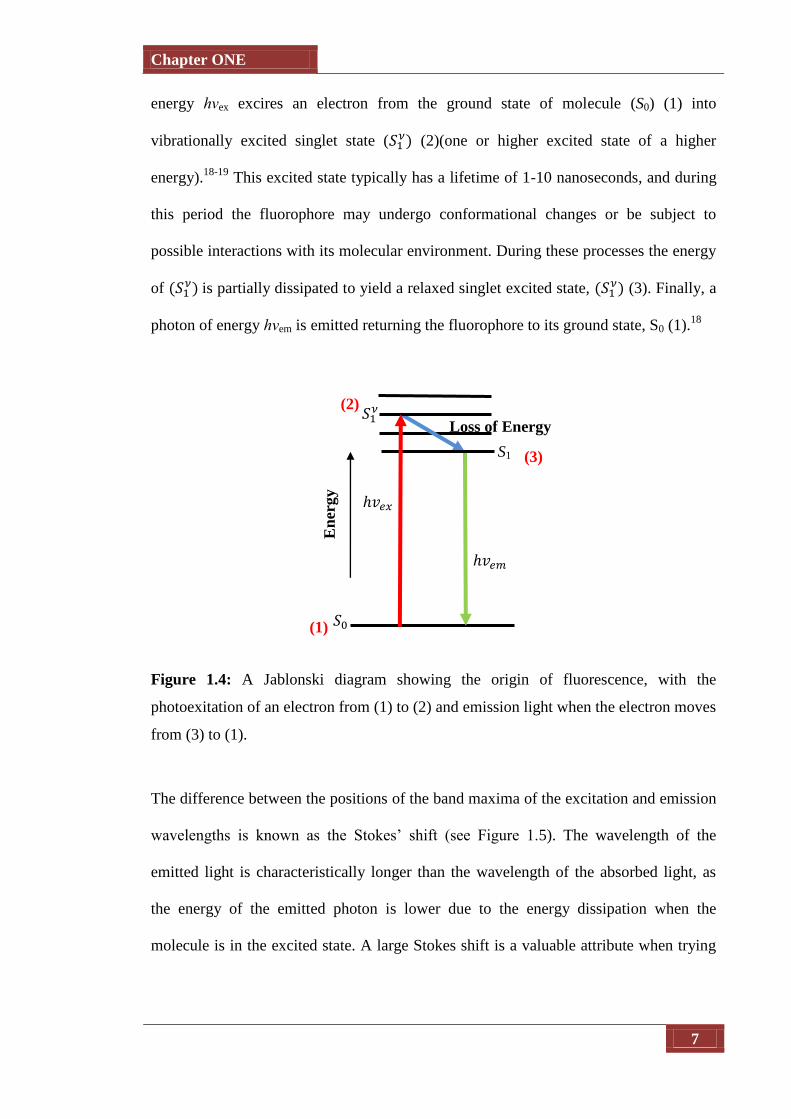
involved in fluorescence is shown in a Jablonski diagram in Figure 1.4. A photon of
Stack
Z-Stack
Chapter ONE
7
energy hνex excires an electron from the ground state of molecule (S0) (1) into
vibrationally excited singlet state ( (2)(one or higher excited state of a higher
energy).18-19
This excited state typically has a lifetime of 1-10 nanoseconds, and during
this period the fluorophore may undergo conformational changes or be subject to
possible interactions with its molecular environment. During these processes the energy
of is partially dissipated to yield a relaxed singlet excited state,
(3). Finally, a
photon of energy hνem is emitted returning the fluorophore to its ground state, S0 (1).18
Figure 1.4: A Jablonski diagram showing the origin of fluorescence, with the
photoexitation of an electron from (1) to (2) and emission light when the electron moves
from (3) to (1).
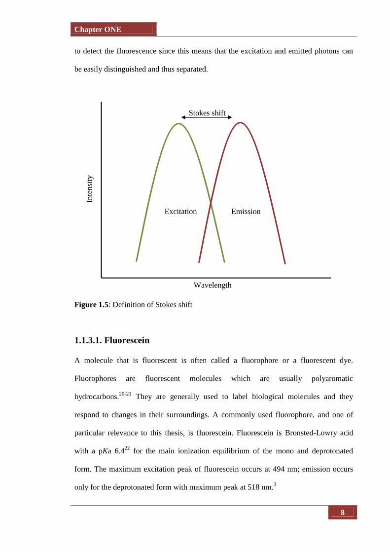
The difference between the positions of the band maxima of the excitation and emission
wavelengths is known as the Stokes’ shift (see Figure 1.5). The wavelength of the
emitted light is characteristically longer than the wavelength of the absorbed light, as
the energy of the emitted photon is lower due to the energy dissipation when the
molecule is in the excited state. A large Stokes shift is a valuable attribute when trying
En
ergy
S1
Loss of Energy
(2)
(3)
(1)
Chapter ONE
8
to detect the fluorescence since this means that the excitation and emitted photons can
be easily distinguished and thus separated.
Figure 1.5: Definition of Stokes shift
1.1.3.1. Fluorescein
A molecule that is fluorescent is often called a fluorophore or a fluorescent dye.
Fluorophores are fluorescent molecules which are usually polyaromatic
hydrocarbons.20-21
They are generally used to label biological molecules and they
respond to changes in their surroundings. A commonly used fluorophore, and one of
particular relevance to this thesis, is fluorescein. Fluorescein is Bronsted-Lowry acid
with a pKa 6.422
for the main ionization equilibrium of the mono and deprotonated
form. The maximum excitation peak of fluorescein occurs at 494 nm; emission occurs
only for the deprotonated form with maximum peak at 518 nm.3
Wavelength
Inte
nsi
ty
Excitation Emission
Stokes shift
Chapter ONE
9
(1.1)
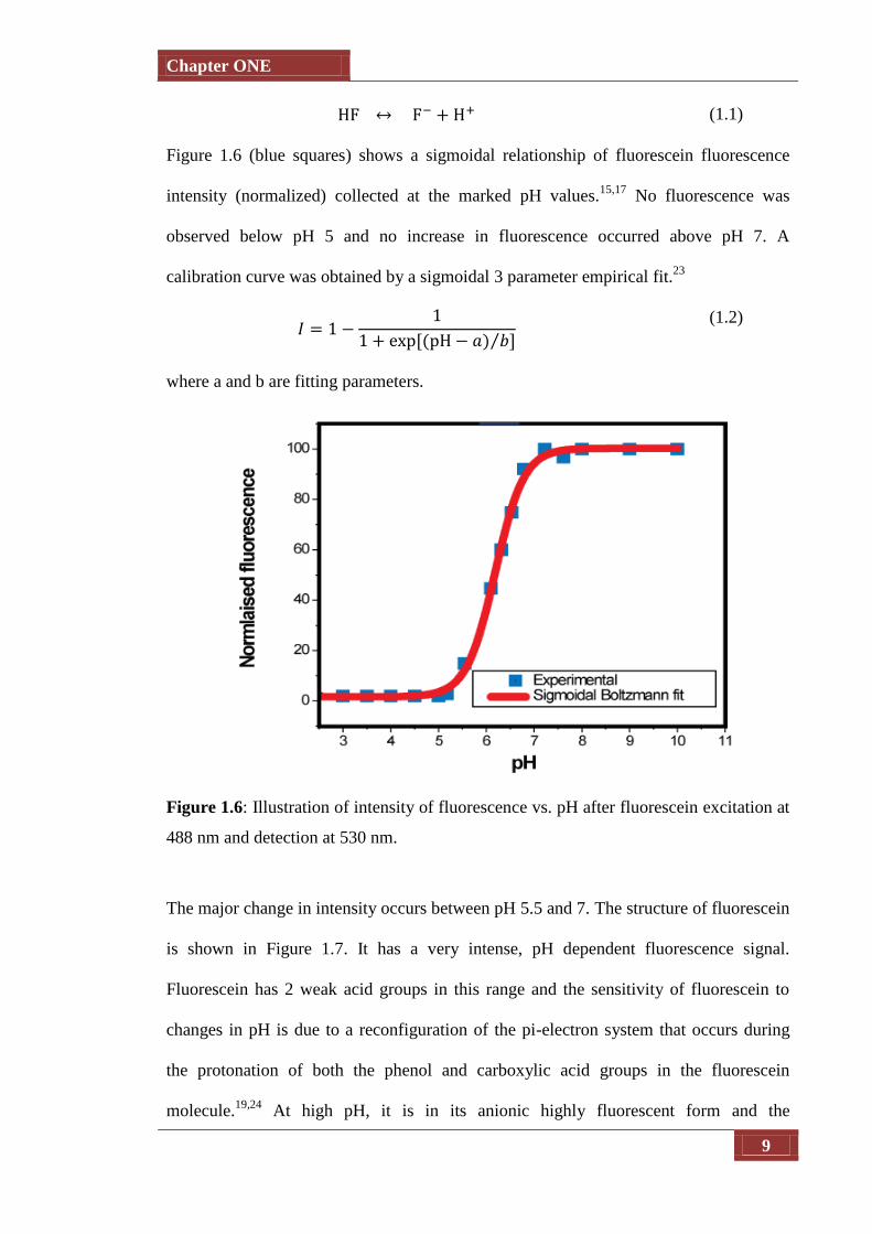
Figure 1.6 (blue squares) shows a sigmoidal relationship of fluorescein fluorescence
intensity (normalized) collected at the marked pH values.15,17
No fluorescence was
observed below pH 5 and no increase in fluorescence occurred above pH 7. A
calibration curve was obtained by a sigmoidal 3 parameter empirical fit.23
⁄
(1.2)
where a and b are fitting parameters.
Figure 1.6: Illustration of intensity of fluorescence vs. pH after fluorescein excitation at
488 nm and detection at 530 nm.
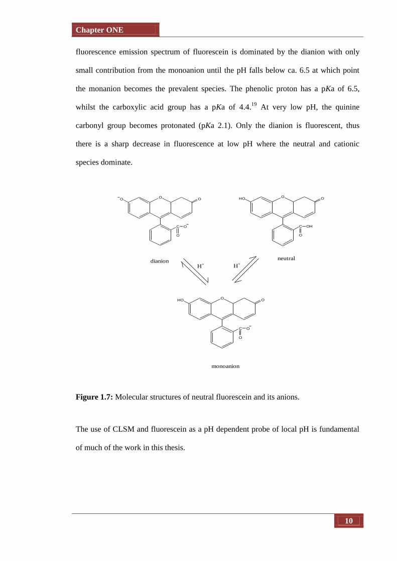
The major change in intensity occurs between pH 5.5 and 7. The structure of fluorescein
is shown in Figure 1.7. It has a very intense, pH dependent fluorescence signal.
Fluorescein has 2 weak acid groups in this range and the sensitivity of fluorescein to
changes in pH is due to a reconfiguration of the pi-electron system that occurs during
the protonation of both the phenol and carboxylic acid groups in the fluorescein
molecule.19,24
At high pH, it is in its anionic highly fluorescent form and the
Chapter ONE
10
fluorescence emission spectrum of fluorescein is dominated by the dianion with only
small contribution from the monoanion until the pH falls below ca. 6.5 at which point
the monanion becomes the prevalent species. The phenolic proton has a pKa of 6.5,
whilst the carboxylic acid group has a pKa of 4.4.19
At very low pH, the quinine
carbonyl group becomes protonated (pKa 2.1). Only the dianion is fluorescent, thus
there is a sharp decrease in fluorescence at low pH where the neutral and cationic
species dominate.
Figure 1.7: Molecular structures of neutral fluorescein and its anions.
The use of CLSM and fluorescein as a pH dependent probe of local pH is fundamental
of much of the work in this thesis.
O OHO
C
O
OH
O OHO
C
O
O
O OO
C
O
O
dianion neutral
monoanion
H+ H
+
Chapter ONE
11
1.2. Electrochemistry and Microelectrodes
1.2.1. Introduction to electrochemistry
The simplest electrode system is when a metal (or object) is placed in an electrolyte
solution. This results in charge transfer at the interface between the electrode and the
electrolyte, where gradients in electrical and chemical potentials constitute the driving
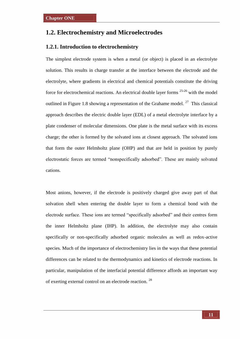
force for electrochemical reactions. An electrical double layer forms 25-26
with the model
outlined in Figure 1.8 showing a representation of the Grahame model. 27
This classical
approach describes the electric double layer (EDL) of a metal electrolyte interface by a
plate condenser of molecular dimensions. One plate is the metal surface with its excess
charge; the other is formed by the solvated ions at closest approach. The solvated ions
that form the outer Helmholtz plane (OHP) and that are held in position by purely
electrostatic forces are termed “nonspecifically adsorbed”. These are mainly solvated
cations.
Most anions, however, if the electrode is positively charged give away part of that
solvation shell when entering the double layer to form a chemical bond with the
electrode surface. These ions are termed “specifically adsorbed” and their centres form
the inner Helmholtz plane (IHP). In addition, the electrolyte may also contain
specifically or non-specifically adsorbed organic molecules as well as redox-active
species. Much of the importance of electrochemistry lies in the ways that these potential
differences can be related to the thermodynamics and kinetics of electrode reactions. In
particular, manipulation of the interfacial potential difference affords an important way
of exerting external control on an electrode reaction. 28
Chapter ONE
12
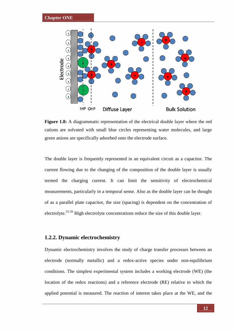
Figure 1.8: A diagrammatic representation of the electrical double layer where the red
cations are solvated with small blue circles representing water molecules, and large
green anions are specifically adsorbed onto the electrode surface.
The double layer is frequently represented in an equivalent circuit as a capacitor. The
current flowing due to the changing of the composition of the double layer is usually
termed the charging current. It can limit the sensitivity of electrochemical
measurements, particularly in a temporal sense. Also as the double layer can be thought
of as a parallel plate capacitor, the size (spacing) is dependent on the concentration of
electrolyte.25-26
High electrolyte concentrations reduce the size of this double layer.
1.2.2. Dynamic electrochemistry
Dynamic electrochemistry involves the study of charge transfer processes between an
electrode (normally metallic) and a redox-active species under non-equilibrium
conditions. The simplest experimental system includes a working electrode (WE) (the
location of the redox reactions) and a reference electrode (RE) relative to which the
applied potential is measured. The reaction of interest takes place at the WE, and the

Chapter ONE
13
reference electrode is chosen to have constant composition, and therefore a fixed
potential.28
Where the typical current is expected to be greater than about 100 nA, a 3-
electrode set-up is required. This introduction of a counter electrode is necessary as such
large currents would otherwise perturb the fixed potential of the reference electrode and
render it unstable (due to electrolysis of its components).28
Measurement of the current that flows provides information on the solution, the
electrodes and the interfacial reactions. The rate of the WE reaction is influenced by
several factors, including the rate of the electron transfer at the electrode surface, mass
transport of the redox-active species to the electrode, chemical reactions in the solution,
the nature of the electrode surface, and the structure of the interfacial region over which
the reaction occurs.
Figure 1.9: The effect of the applied potential on the Fermi level.27
Potential applied
Negative
Fermi level
Positive
Metal
Reactant
HOMO
LUMO
Energy

Chapter ONE
14
The maximum of the continuum is known as the Fermi level. Application of a potential
to the WE, with respect to the RE, can change the Fermi level of the metal used as the
electrode (see Figure 1.9). While the Fermi level is of an energy between that of the
lowest unoccupied molecular orbital (LUMO) and the highest occupied molecular
orbital (HOMO), no electron transfer will occur. If a sufficiently negative potential is
applied, the Fermi level increases in energy such that it is above the LUMO. In this
situation, electron transfer occurs from the metal to the reactant, causing reduction of
the reactant. Conversely, if a sufficiently positive potential is applied, the Fermi level
decreases in energy such that it is below the HOMO. Electron transfer proceeds from
the reactant to the metal electrode, leading to oxidation of the reactant.27
Figure 1.10: A schematic representation of a typical electrode reaction.28
The reaction rate of a typical electrode reaction involves several steps, which are
illustrated schematically in Figure 1.10. The overall reaction rate is limited by the
slowest step. It is often the case that the applied potential is increased to such an extent
that the electron transfer process occurs more rapidly than material can be transported to

Chapter ONE
15
or from the electrode. Under these conditions, the current response is limited by the rate
of mass transport,27
which is the subject of the next section. More complex reactions
may involve chemical reactions in solution, either before or after electron transfer, and
surface reactions such as adsorption or desorption. Protonation is a common chemical
reaction that is often coupled to electron transfer which leads to the production of pH
gradients between the interfacial region and bulk solution, if the solution is not buffered.
The aim of this thesis is to image and quantify the pH gradients that develop at active
surfaces. These can arise either through chemical reactions in solution or electrode
reactions that produce or consume protons or hydroxide ions, for example tris(2,2'-
bipyridine)ruthenium(II) oxidation (chapter 3) and water oxidation (chapter 4 and 5).
1.2.3. Mass transport
Mass transfer of dilute species in solution is governed by the Nernst-Planck equation28
and for one-dimensional mass transfer along the x-axis the expression is as follows:
(1.3)
where Jj is the flux (i.e. the number of moles passing through a given area per unit time)
of species j to/from the electrode, Dj is the diffusion coefficient of species j, cj is the
concentration of species j, V is the velocity vector, zj is the charge on species j, F is the
Faraday’s constant, R is the gas constant, T is temperature and φ is the electrostatic
potential. The three terms on the right hand side represents the contributions of
diffusion, convection, and migration, respectively, to the flux.25
Thus, the factors contributing to mass transport include diffusion (movement along a
concentration gradient), convection (the directed movement of the solution itself
Chapter ONE
16
carrying the species) and migration of the species (for example, the directed motion of
ions due to some applied electrostatic potential).28
An increase in any of these factors
can promote mass transport, alleviating them as a possible rate limiting factor in
reactions with fast electrode surface kinetics. Addition of a background electrolyte to a
cell minimises any effects from migration, and can aid eliminating the development of
liquid junction potential and prevent any contributions from ohmic drop by decreasing
the resistivity of the solution. The background electrolyte does not take part/ interfere in
the reaction occurring at the tip of WE but does decreases the size of the double layer at
the electrode/surface interface; where a small double layer results in a high electric
field, ensuring that the full potential applied at the electrode is available for the
electrochemical process.28-29
Experimental conditions can be chosen so that no significant contribution is made by
convection and migration so that diffusion is dominant (as discussed above). Thus, all
mass transport models of fluxes in this thesis make use of only the diffusive aspects of
the Nernst- Planck equation, significantly simplifying any numerical analysis of
experimental results. To precisely quantify electrode reactions, it is necessary to take
each aspect of mass transport into consideration.
1.2.3.1. Diffusion
Diffusion is always present in a dynamic electrode process and is defined as the
movement of a species down a concentration (formally, activity) gradient, due to the
difference in concentration (activity) of the species at the electrode surface and the bulk
solution. Diffusion is described mathematically by Fick’s laws28
, the first of which
Chapter ONE
17
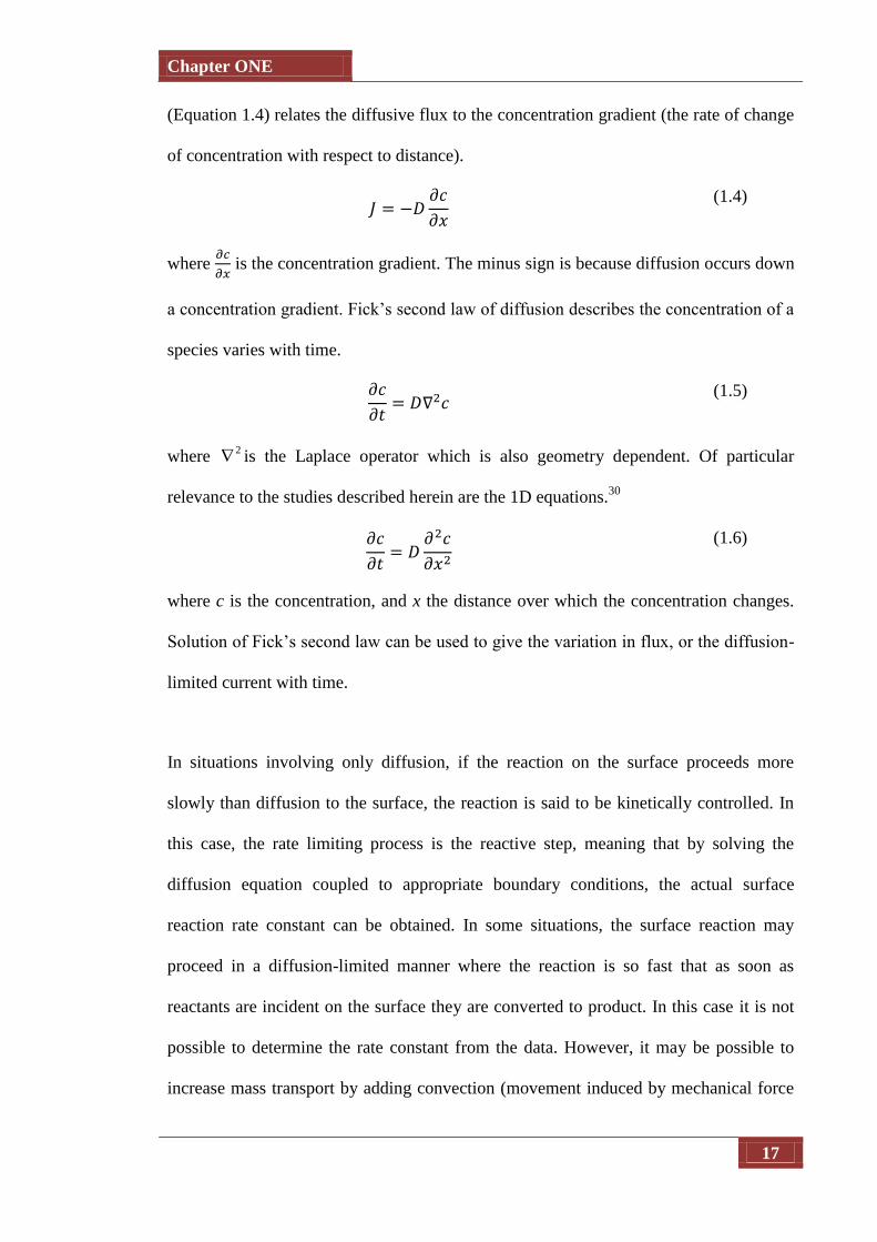
(Equation 1.4) relates the diffusive flux to the concentration gradient (the rate of change
of concentration with respect to distance).
(1.4)
where
is the concentration gradient. The minus sign is because diffusion occurs down
a concentration gradient. Fick’s second law of diffusion describes the concentration of a
species varies with time.
(1.5)
where 2 is the Laplace operator which is also geometry dependent. Of particular
relevance to the studies described herein are the 1D equations.30
(1.6)
where c is the concentration, and x the distance over which the concentration changes.
Solution of Fick’s second law can be used to give the variation in flux, or the diffusion-
limited current with time.
In situations involving only diffusion, if the reaction on the surface proceeds more
slowly than diffusion to the surface, the reaction is said to be kinetically controlled. In
this case, the rate limiting process is the reactive step, meaning that by solving the
diffusion equation coupled to appropriate boundary conditions, the actual surface
reaction rate constant can be obtained. In some situations, the surface reaction may
proceed in a diffusion-limited manner where the reaction is so fast that as soon as
reactants are incident on the surface they are converted to product. In this case it is not
possible to determine the rate constant from the data. However, it may be possible to
increase mass transport by adding convection (movement induced by mechanical force

Chapter ONE
18
e.g. stirring), causing the reaction to become kinetically controlled as discussed in the
next section.
1.2.3.2. Convection
Convection is the movement of species in a fluid due to an external mechanical force.
The convective component of flux is given by:
(1.7)
There are two types of convection. The first is natural convection, which can be present
in any solution and arises from thermal gradients and/or density differences within the
solution. Forced convection is normally orders of magnitude larger than natural
convection, and so obscures any effect that natural convection may have. It arises when
the solution is deliberately agitated which can be achieved in several different ways,
leading to a multitude of convective (or hydrodynamic) systems.31
In some
electrochemical experiments an element of forced convection is deliberately introduced
to swamp any contribution from natural convection, ensuring that reproducible
experiments can be made over extended time-scales. Forced convection is usually
achieved by external forces such as gas bubbling through solution, pumping, or
stirring.28
1.2.3.3. Migration
From equation 1.1 it is apparent that migration only affects species which are charged. It
is the movement of charged species under the influence of an external electric field
(∂φ/∂x). Migrative flux is described by:
(1.8)

Chapter ONE
19
Due to the difficulty in quantifying its effect, migration is often removed during
electrochemical experiments by the addition of an excess concentration of an inert
supporting electrolyte.28
As already mentioned, this also has the benefit of reducing the
effect of uncompensated (Ohmic) resistance and compressing the size of the electrical
double layer, such that the potential across the electrode/solution interface drops over a
distance commensurate with electron transfer.26,28
All studies in this thesis are carried
out under conditions where migration can be ignored.
1.2.4 Ultramicroelectrodes (UMEs)
There are various types of electrodes employed and the critical factor determining their
behaviour is the interplay between mass transport to the electrode and the electron
transfer kinetics. The former may be directly linked to their size. Macroelectrodes have
dimensions of the order of centimetres or millimetres; when one of the critical
dimensions of the electrode is in the micrometer range, the electrode behaves as an
ultramicroelectrode (UME).32-35
Ultramicroelectrodes, UMEs, have been widely used and characterised since the 1970’s
when it became apparent that electrodes of this type eliminated many of the unwanted
characteristics of larger macro-electrodes, discussed below.33,36-37
UME probes are
generally fabricated using platinum, palladium, gold, silver wires or carbon fused into
glass or embedded in plastic.38-40
An electrical contact is then made by polishing away
the extremity of the insulator to reveal the electrode material. Characterisation is often
achieved using two electrochemical techniques: cyclic voltammetry (CV), and scanning
electrochemical microscopy (SECM) in conjunction with optical microscopy.39-40
These

Chapter ONE
20
techniques and their application in the characterisation of UMEs are discussed in
sections 1.2.5.1and 1.2.6, respectively.
The exposed part of the metal can take different forms (Figure 1.14),37,41
depending on
the application42
and on the method of fabrication such as: disc electrodes,43
array, 44-45
band,46-47
hemisphere, cylinder, spherical mercury electrodes,48-49
ring electrodes,50-51
and carbon fibre electrodes52-53
ring,54-55
but by far the most widely used is the disc
electrode since its fabrication is relatively straight forward, the sensing area can be
polished mechanically and it is easily modellable. The diffusion fields, which promote
the movement of materials to and from the electrode, are dependent on the shape of the
electrode and the timescale of the measurement. Diffusion processes that take place are
shown schematically in Figure 1.11. All show substantial “edge effects” which lead to
the enhanced mass transport rates.41
Figure 1.11: Different geometries of electrodes and their diffusion fields: (a) Disk
electrode (b) Cylinder electrode and (c) Ring electrode. Reproduced from reference.41
The size of the working electrode is an important consideration in electrochemical
experiments. First, we should consider the traditional macroelectrode. Diffusion to this
type of electrode is predominately planar, as shown in Figure 1.12(a). In contrast, the
small size of UMEs results in extremely efficient diffusional mass transport due to the
Disc electrode Cylinder electrode Ring electrode
a) b) c)
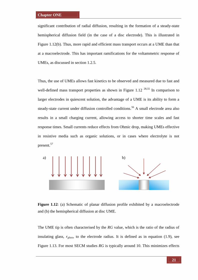
Chapter ONE
21
significant contribution of radial diffusion, resulting in the formation of a steady-state
hemispherical diffusion field (in the case of a disc electrode). This is illustrated in
Figure 1.12(b). Thus, more rapid and efficient mass transport occurs at a UME than that
at a macroelectrode. This has important ramifications for the voltammetric response of
UMEs, as discussed in section 1.2.5.
Thus, the use of UMEs allows fast kinetics to be observed and measured due to fast and
well-defined mass transport properties as shown in Figure 1.12 28,55
In comparison to
larger electrodes in quiescent solution, the advantage of a UME is its ability to form a
steady-state current under diffusion controlled conditions.56
A small electrode area also
results in a small charging current, allowing access to shorter time scales and fast
response times. Small currents reduce effects from Ohmic drop, making UMEs effective
in resistive media such as organic solutions, or in cases where electrolyte is not
present.57
Figure 1.12: (a) Schematic of planar diffusion profile exhibited by a macroelectrode
and (b) the hemispherical diffusion at disc UME.
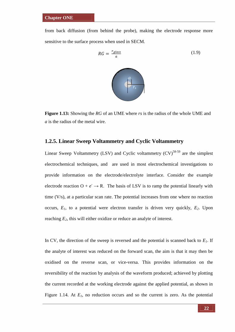
The UME tip is often characterised by the RG value, which is the ratio of the radius of
insulating glass, rglass, to the electrode radius. It is defined as in equation (1.9), see
Figure 1.13. For most SECM studies RG is typically around 10. This minimizes effects
a) b)
Chapter ONE
22
from back diffusion (from behind the probe), making the electrode response more
sensitive to the surface process when used in SECM.
(1.9)
Figure 1.13: Showing the RG of an UME where rs is the radius of the whole UME and
a is the radius of the metal wire.
1.2.5. Linear Sweep Voltammetry and Cyclic Voltammetry
Linear Sweep Voltammetry (LSV) and Cyclic voltammetry (CV)58-59
are the simplest
electrochemical techniques, and are used in most electrochemical investigations to
provide information on the electrode/electrolyte interface. Consider the example
electrode reaction O + e- → R. The basis of LSV is to ramp the potential linearly with
time (V/s), at a particular scan rate. The potential increases from one where no reaction
occurs, E1, to a potential were electron transfer is driven very quickly, E2. Upon
reaching E2, this will either oxidize or reduce an analyte of interest.
In CV, the direction of the sweep is reversed and the potential is scanned back to E1. If
the analyte of interest was reduced on the forward scan, the aim is that it may then be
oxidised on the reverse scan, or vice-versa. This provides information on the
reversibility of the reaction by analysis of the waveform produced; achieved by plotting
the current recorded at the working electrode against the applied potential, as shown in
Figure 1.14. At E1, no reduction occurs and so the current is zero. As the potential
a
rs

Chapter ONE
23
increases, the rate of reduction increases, and so the current increases approximately
exponentially with increasing potential (and thus time), as predicted by the Butler-
Volmer equation.29
The current reaches a maximum value and a peak is seen. This
occurs because the current depends not only on the rate constant for reduction, kred, but
also on the surface concentration of the redox species.
Figure 1.14: Typical CV responses for (a) a macroelectrode and (b) an
ultramicroelectrode.
Once this peak in the current is reached, the current is limited by the rate of mass
transport (i.e. diffusion) of reactant to the electrode surface. The fall in current that
occurs is due to an increase in the depth of the depleted region next to the electrode and
the inability of mass transfer to compete with the rate of electron transfer. Once the
sweep reaches the switching potential, E2, the potential reverses and the reaction
proceeds in the opposite direction. The voltammogram takes the form of a mirror image
of the forward sweep, but is shifted by 59/n mV, as dictated by the Nernst equation for
the case of a completely reversible.28
The scan rate plays an important role in the
magnitude of the current. A typical voltammogram obtained for a macroelectrode is
shown in Figure 1.14(a).
b)
a)
i i
E E
Chapter ONE
24
The cyclic voltammogram observed for a UME takes a different form to that described
above for a traditional macroelectrode (Figure 1.14) for relatively low scan rate. Instead
of the peaked reponse, the voltammogram takes a sigmoidal shape, as shown in Figure
1.14(b). A maximum value of the current is observed, and the voltammogram plateaus
at this value. This is termed the diffusion-limited current. This value of the current is
maintained due to efficient replenishment of reactant at the electrode surface, resulting
from rapid hemispherical diffusion to the UME. This bulk steady-state limiting current,
for a disc UME can be theoretically calculated from Equation 1.10.25,60
(1.10)
where n is the number of electrons transferred in the electrode reaction, a is the
electrode radius, c* is the bulk concentration of the electroactive species and K is a
geometrydependent constant (K is 4 for a disc UME or 2π for a hemispherical UME).
Comparison of theoretical and experimental currents gives a quick indication that the
system is working correctly. The shape of the sigmoidal waveform can be used to verify
the electrode properties, e.g. the diameter of the active metal, the shape of the UME and
how well the wire is sealed to the glass; and can be used to judge how good an electrode
is. Both potential and scan rate can be controlled through a potentiostat, which monitors
the potential applied to the tip and records the current response.
A galvanostat can also be employed to generate currents at the tip of the UME. This
operates by varying the potential to maintain and monitor a controlled current. In
principle, a galvanostat can act as a potentiostat and vice-versa, depending on how the
cell is connected, however some models of potentiostat already have this feature built-
in.25-26

Chapter ONE
25
1.2.6. Scanning electrochemical microscopy (SECM)
SECM is a powerful scanned probe technique for quantitative investigations of
interfacial physicochemical processes, in a wide variety of areas, as considered in
several recent reviews.61-62
In the simplest terms, SECM involves the use of a mobile
ultramicroelectrode (UME) probe, either amperometric or potentiometric, to investigate
the activity and/or topography of an interface on a localized scale; typically resolution is
on a micron length scale. It is capable of delivering a reagent to a surface with high rates
of mass transport,28,63
and is highly controlled64-69
allowing the characterization of fast
surface processes and the ability to study the chemical reactivity of analyte.70-79
A
comprehensive review of all these aspects can be found in Bard and Mirkin.38
SECM involves monitoring the current generated at a tip as it is scanned across or
towards a sample.80
The SECM tip is attached to a precise piezoelectric positioning
system which allows the tip to be moved in the x, y or z-direction with submicron-scale
precision.40
Undoubtedly, the most crucial component of the SECM is the tip. A
commonly used tip is based on an embedded disk-shaped geometry.63
The tip typically
consists of a disc UME surrounded by an insulating glass sheath. The quantity of glass
surrounding the electrode can affect the current response obtained in certain cases.
Because of this, the electrode is characterised by an RG value 8, as defined in section
1.2.4. At RG values below 10, back diffusion increasingly influences the currents seen.
Exceeding an RG of 10 tends to largely eliminate these effects. The UME is immersed
into a liquid phase and then placed close to another phase, which could be solid, liquid
or gas. A potential is applied to the UME as it is scanned across or moved towards the
interface of interest. The current response of the UME can give a great deal of
information about the topography and the chemical reactivity of the surface.27

Chapter ONE
26
The advantages of SECM are that it is typically a non-invasive, non-destructive
technique. It is well suited to small volumes where reactions can be detected directly
and it allows the study of interfacial kinetic processes due to the high rates of mass
transport achievable. It has high spatial resolution, versatility and selectivity. It is well
known for chemical mapping and is used to investigate surface topography.81-82
As
examples, the technique has been applied to air/water interfaces to study gas
permeation,83
liquid/liquid interfaces,61,84-90
liquid/solid interfaces,68,91
single crystal,65-
67,92-93 and porous membranes.
94-95
Chapter 4 and 5 outlines some further examples of SECM applications applicable to the
work herein, in the fields of dissolution processes, kinetics and proton dispersion at
many interfaces. Several modes of SECM have been developed to allow the local
chemical properties of interfaces to be investigated. The mode of SECM most relevant
to this work is the feedback mode.96
There are basically two forms: negative feedback
and positive feedback.63
In this work, SECM is employed in the feedback mode to
obtain approach curves to the surface of interest in order to determine UME-surface
separation distance (chapters 4 and 5).
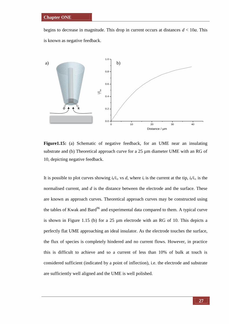
1.2.6.1 Negative Feedback
Negative feedback, where a UME approaches an insulating substrate, is shown in Figure
1.15(a). A potential is applied to the UME in order to reduce electroactive species O
(present in solution) to species R at a diffusion limited rate, which generate a current, i∞,
at the tip electrode. As the tip approaches an insulating (inert) substrate, the
hemispherical diffusion to the tip becomes hindered, and as such the current generated
Chapter ONE
27
begins to decrease in magnitude. This drop in current occurs at distances d < 10a. This
is known as negative feedback.
Figure1.15: (a) Schematic of negative feedback, for an UME near an insulating
substrate and (b) Theoretical approach curve for a 25 µm diameter UME with an RG of
10, depicting negative feedback.
It is possible to plot curves showing it/i∞ vs d, where it is the current at the tip, it/i∞ is the
normalised current, and d is the distance between the electrode and the surface. These
are known as approach curves. Theoretical approach curves may be constructed using
the tables of Kwak and Bard96
and experimental data compared to them. A typical curve
is shown in Figure 1.15 (b) for a 25 µm electrode with an RG of 10. This depicts a
perfectly flat UME approaching an ideal insulator. As the electrode touches the surface,
the flux of species is completely hindered and no current flows. However, in practice
this is difficult to achieve and so a current of less than 10% of bulk at touch is
considered sufficient (indicated by a point of inflection), i.e. the electrode and substrate
are sufficiently well aligned and the UME is well polished.
0 10 20 30 40
0.0
0.2
0.4
0.6
0.8
1.0
i t/i lim
Distance / µm
a) b)

Chapter ONE
28
1.2.6.2. Positive Feedback
Positive feedback63,96
occurs when the UME approaches a conducting substrate as
shown in Figure 1.16 (a). In this situation, when the UME reaches a certain tip-surface
separation, species R which has been generated at the tip is oxidised back to species O
at the surface. This leads to an increasing concentration of species O being provided for
reduction at the UME, and, as such, an increase in the current is seen. This is termed
positive feedback. Theoretical approach curves for conducting surfaces can be plotted in
a similar manner to those for insulating surfaces, discussed in section 2.2.1. The
theoretical approach curve for a conducting substrate is given in Figure 1.16 (b) using a
25 µm diameter electrode with an RG of 10.
Figure 1.16: (a) Schematic of positive feedback near a conducting substrate (b)
Theoretical approach curve for a 25 µm diameter UME displaying positive feedback.
1.4. Finite Element Modelling (FEM)
The simulation in this thesis was performed using the commercially available software
package, Comsol Multiphysics. This environment provides the user with all of the
0 1 2 3 4 5 6 7 8 9
0
1
2
3
4
5
6
7
8
9
i t/ilim
Distance / µm
a) b)

Chapter ONE
29
advantages of FEM, but a detailed knowledge of the complex mathematics behind this
method is not required. It combines these advantages with an extremely user-friendly
interface that enables simple construction of complex geometries (in one-, two- or three-
dimensions) and simple definition of governing equations and boundary conditions.
Many equations commonly used in the fields of engineering and physics are already
built into the program (including diffusion, diffusion-convection and the Navier-Stokes
equations for incompressible flow which are of relevance to this thesis) but a generic
module is also present so that user defined equations can also be solved.
Essentially, COMSOL Multiphysics provides approximate solutions to differential
equations using the finite element method. This technique uses a computer to solve a
defined set of equations (i.e. Fick’s second law of diffusion and Navier-Stokes
equations for the work within this thesis) within a user defined domain. In 2D
simulations applied herein the problem is broken down into a set of triangular elements,
known as a mesh, which is used to approximate the domain being simulated (Figure
1.17(a)).97-98
Generating a mesh the chosen equations are calculated at the corners of
each triangular element. For areas where the result is likely to change the most, for
example a concentration gradient near an electrode surface, the mesh density is
increased (Figure 1.17 (b)). This can be either defined by the user or using an algorithm
to focus on areas of greatest change in a property (e.g. fluid velocity and concentration).
Both mesh refinement approaches allow simulations to be run efficiently without
sacrificing accuracy.99-101

Chapter ONE
30
Figure 1.17: (a) An example of a simple triangular mesh used for FEM and (b) the
same domain where the mesh is finer at two edges.
Many systems have used finite element models as a means of aiding understanding of
reactions processes, mechanisms or kinetics.97,102-103
In electrochemistry, FEM has been
used both through self-written programs and commercially available software packages.
In fact, one of the seminal SECM theory paper by Kwak and Bard,63
describing the
positive and negative feedback response expected during an approach curve
measurement, relied on finite element simulations. With particular relevance to SECM,
models have been used to monitor transport through porous membranes, 104
to
understand catalytic processes,105
and to develop tip positioning.106
Other researchers
have used models to visualise the permeability of films107
and to define kinetics.108-109
For the work in this thesis and resulting publications, finite element models were
created by a colleague, Dr. Martin Edwards to produce the theoretical characteristics
and a fundamental understanding of the reaction processes occurring in solution. This
aspect is described in more detail in Chapter 4 where boundary conditions and
experimental parameters are also defined.
b) a)

Chapter ONE
31
1.5. Aims of this Thesis
The overarching aim of thesis is to develop a new understanding of physiochemical
processes and diffusion problems at interfaces by developing new techniques and
exploring wider applications, which can be summarised as follows:
The main goal is to demonstrate the use of fluorescence CLSM coupled with
electrochemical techniques and finite element modelling (through Comsol
Multiphysics) in the quantification of concentration and pH gradients produced upon
reaction at an electrode. The concentration gradient determined directly, while pH
gradients are visualised through the addition of trace amounts of fluorescein, a dye that
has a pH-dependent fluorescent signal. The fluorescence profile is predicted through
simulation of the underlying mass transport equations.
Following on from the introduction, the apparatus used, experimental details and set-up
are given in Chapter 2. This includes sample preparation, device microfabrication and
characterisation, CLSM imaging experiments and the additional techniques used.
Chapter 3 includes a discussion on combining electrochemical investigation with
fluorescence confocal laser scanning microscopy (CLSM) imaging to assess the
usability of CNTs mats as disc OT-UMEs. Simultaneous monitoring of redox reactions
is possible by using fluorophore the luminescent properties of which depend on either
solution pH or fluorophore redox state. In this study a ST-cut quartz substrate is
employed to grow ultrathin films of interconnected CNTs at optimised cCVD
conditions utilising ethanol and cobalt as carbon feedstock and catalyst, respectively.
Chapter ONE
32
Chapter 4 describes the use of confocal microscopy coupled with SECM as a powerful
technique for direct visualisation of acid-induced reaction processes and as a method for
assessing the effectiveness of protective barriers on the enamel surface. It details the
effect that fluoride and zinc treated enamel have on the prevention of acid attack. This
found that Zn2+
treatment provides a much better barrier to prevent acid attack on
enamel.
Chapter 5 investigates the lateral diffusion of protons through bilayer lipid membranes
by the CLSM-SECM technique. A UME is brought close to the bilayer and
galvanostatic water oxidation is induced, generating a proton gradient near the
membrane. The transport of protons is observed as a pH change alongside bilayer. The
effect of different ionisable head group, such as acidic distearoyl phosphatidylglycerol
1,2-ditetradecanoyl-sn-glycero-3-phospho-(1'-rac-glycerol) (DSPG) and zwitterionic
phosphatidyl choline (EPC), on this process is also studied since it is thought that such
negatively charged lipids facilitate proton lateral diffusion.
Finally, chapter 6 summarises the conclusions drawn and indicates potential directions
for future study.
Chapter ONE
33
1.6. References
(1) Amos, W. B.; White, J. G. Biology of the Cell 2003, 95, 335.
(2) Cox, G. Materials today 2002, 34.
(3) C.J.R.Sheppard; D.M.Shotton Confocal laser scanning microscopy; First ed.;
BIOS Scientific Publisher Limited: Untied States of America, 1997.
(4) Minsky, M. 1957, 7, 107
(5) Webb, R. H. Reports on Progress in Physics 1996, 59, 427.
(6) Halbhuber, K. J.; Konig, K. Annals of Anatomy-Anatomischer Anzeiger 2003,
185, 1.
(7) Nathan S. Claxton, T. J. F., and Michael W. Davidson.
(8) Rudd, N. C., The University of Warwick, 2007.
(9) Amatore, C.; Chovin, A.; Garrigue, P.; Servant, L.; Sojic, N.; Szunerits, S.;
Thouint, L. Analytical Chemistry 2004, 76, 7202.
(10) Foldes-Papp, Z.; Demel, U.; Tilz, G. P. International Immunopharmacology 2003,
3, 1715.
(11) Carlsson, K.; Danielsson, P. E.; Lenz, R.; Liljeborg, A.; Majlof, L.; Aslund, N.
Optics Letters 1985, 10, 53.
(12) Navratil, M.; Mabbott, G. A.; Arriaga, E. A. Analytical Chemistry 2006, 78, 4005.
(13) Fiedler, S.; Hagedom, R.; Schnelle, T.; Richter, E.; Wagner, B.; Fuhr, G.
Analytical Chemistry 1995, 67, 820.
(14) Amatore, C.; Bonhomme, F.; Bruneel, J. L.; Servant, L.; Thouin, L. Journal of
Electroanalytical Chemistry 2000, 484, 1.
(15) Rudd, N. C.; Cannan, S.; Bitziou, E.; Ciani, L.; Whitworth, A. L.; Unwin, P. R.
Analytical Chemistry 2005, 77, 6205.
(16) Grime, J. M. A.; Edwards, M. A.; Rudd, N. C.; Unwin, P. R. Proceedings of the
National Academy of Sciences of the United States of America 2008, 105, 14277.
(17) Cannan, S.; Macklam, I. D.; Unwin, P. R. Electrochemistry Communications
2002, 4, 886.
(18) Lichtman, J. W.; Conchello, J. A. Nature Methods 2005, 2, 910.
(19) Haugland, R. P. Molecular Probes Handbook of Fluorescent Probes and
Research Products,; 9 ed.; Molecular Probes: USA, 2002.
(20) Skoog, D. A. W., A. M.; Holler, F. J Fundamentals of Analytical Chemistry; 7th
ed.; Saunders College Publishing: USA, 1996.
(21) Davidson, R. S. Chemical Society Reviews 1996, 25, 241.
(22) Sjoback, R.; Nygren, J.; Kubista, M. Spectrochimica Acta Part A: Molecular and
Biomolecular Spectroscopy 1995, 51, L7.
(23) Marquardt, D. W. the Society for Industrial and Applied Mathematics 1936, 11,
431.
(24) Diehl, H.; Markuszewski, R. Talanta 1985, 32, 159.
(25) Bard, A. J.; Faulkner, L. R. Electrochemical Methods: Fundamentals and
Applications; 2nd Edition ed.; John Wiley & Sons, Inc.: U.S.A., 2001.
(26) Brett, C. M. A.; Brett, A. M. O. Electrochemistry: Principles, Methods, and
Applications; Oxford University Press: U.K., 2004.
(27) Fisher, A. C. Electrode Dynamics 4ed. Oxford UK, 2006.
(28) Bard, A. J.; Faulkner, L. R. Electrochemical Methods. Fundamentals and
Applications; 2ed ed.; Wiley: India, 2006.
(29) C.M.A. Brett, A.M.O. Brett Electrochemistry: Principles, Methods and
Applications; Oxford University Press: Oxford, 2000, p. 74.
Chapter ONE
34
(30) Donea, J.; Huerta, A.; Ponthot, J.-P.; Rodriguez-Ferran, A. Encyclopedia of
Computational Mechanics, Chapter 14 - Arbitrary Lagrangian-Eulerian Methods;
Wiley and Sons, Ltd, 2004; Vol. 1.
(31) Macpherson, J. V.; Simjee, N.; Unwin, P. R. Electrochimica Acta 2001, 47, 29.
(32) Zoski, C. G. Electroanalysis 2002, 14, 1041.
(33) Heinze, J. Angewandte Chemie-International Edition in English 1993, 32, 1268.
(34) Wightman, R. M. Science 1988, 240, 415.
(35) Fleischmann, M.; Pons, S. Journal of Electroanalytical Chemistry 1989, 261, 301.
(36) Penner, R. M.; Lewis, N. S. Chemistry & Industry 1991, 788.
(37) Forster, R. J. Chemical Society Reviews 1994, 23, 289.
(38) Bard, A. J.; Mirkin, M. V. Scanning Electrochemical Microscopy New York,
2001.
(39) Kwak, J.; Bard, A. J. Analytical Chemistry 1989, 61, 1794.
(40) Bard, A. J.; Fan, F. R. F.; Kwak, J.; Lev, O. Analytical Chemistry 1989, 61, 132.
(41) Unwin, P. R. B., A. J., Stratmann, M., Eds., In In Encyclopedia of
Electrochemistry; Wiley -VCH Weinheim: Germany, 2003; Vol. 3.
(42) R.M. Wightman Science 1988, 240, 415.
(43) R.M. Wightman, D.O. Wipf Electroanalytical Chemistry: A Series of Advances;
A.J. Bard (Ed.), Marcel Dekker: New York, 1989; Vol. 15.
(44) Belal, F.; Anderson, J. L. Analyst 1985, 110, 1493.
(45) Ciszkowska, M.; Stojek, Z. Journal of Electroanalytical Chemistry 1985, 191,
101.
(46) K.R. Wehmeyer, M.R. Deakin, R.M. Wightman Analytical Chemistry 1985, 57,
1913.
(47) T.V. Shea, A.J. Bard Analytical Chemistry 1987, 59, 524.
(48) K.R. Wehmeyer, M.R. Deakin, R.M. Wightman Analytical Chemistry 1985, 57,
1989.
(49) M. Antonietta Baldo, S. Daniele, M. Corbetta, G.A. Mazzocchin Electroanalysis
1995, 7, 980.
(50) D.R. MacFarlane, D.K.Y. Wong Journal of Electroanalytical Chemistry 1985,
185, 197.
(51) M. Fleischmann, S. Bandyopadyhay, S. Pons Journal of Physical Chemistry 1985,
89, 5537.
(52) J.L. Ponchon, R. Cespuglio, F. Gonon, M. Jouvet, J.F. Pujol Analytical Chemistry
1979, 51, 1483.
(53) M.A. Dayton, J.C. Brown, K.J. Stutts, R.M. Wightman Analytical Chemistry
1980, 52, 946.
(54) Wightman, R. M. Analytical Chemistry 1981, 53, 1125.
(55) Woolaston, W. H. Philos. Trans. R. Soc. London. 1801, 91, 427.
(56) Bindra, P.; Brown, A. P.; Fleischmann, M.; Pletcher, D. Journal of
Electroanalytical Chemistry 1975, 58, 31.
(57) Bond, A. M.; Fleischmann, M.; Robinson, J. Journal of Electroanalytical
Chemistry 1984, 180, 257.
(58) Linge, H. G.; Nancolla.Gh Calcified Tissue Research 1973, 12, 193.
(59) Pletcher, D.; Sotiropoulos, S. Journal of Electroanalytical Chemistry 1993, 356,
109.
(60) Saito, Y. Rev. Polarogr. 1968, 15, 177.
(61) Barker, A. L.; Gonsalves, M.; Macpherson, J. V.; Slevin, C. J.; Unwin, P. R.
Analytica Chimica Acta 1999, 385, 223.

Chapter ONE
35
(62) Wittstock, G.; Burchardt, M.; Pust, S. E.; Shen, Y.; Zhao, C. Angewandte Chemie-
International Edition 2007, 46, 1584.
(63) Kwak, J.; Bard, A. J. Analytical Chemistry 1989, 61, 1221.
(64) Macpherson, J., V; Unwin, P., R. Journal of the Chemical Society Faraday
Transactions 1993, 89, 1883.
(65) Macpherson, J. V.; Unwin, P. R. Journal of Physical Chemistry 1994, 98, 1704.
(66) Macpherson, J. V.; Unwin, P. R. Journal of Physical Chemistry 1995, 99, 3338.
(67) Unwin, P. R.; Macpherson, J. V. Chemical Society Reviews 1995, 24, 109.
(68) Macpherson, J. V.; Unwin, P. R. Journal of Physical Chemistry 1995, 99, 14824.
(69) Unwin, P. R.; Macpherson, J. V.; Martin, R. D.; McConville, C. F.
Electrochemical Society 2000, 99, 104.
(70) Amemiya, S.; Bard, A. J.; Fan, F.-R. F.; Mirkin, M.; Unwin, P. R. Analytical
Chemistry 2008, 1, 95.
(71) Barker, A. L.; Gonsalves, M.; Macpherson, J. V.; Slevin, C. J.; Unwin, P. R.
Analytica Chimica Acta 1999, 385, 223.
(72) Wittstock, G.; Burchardt, M.; Pust, S.; Shen, Y.; Zhao, C. Angewandte Chemie
International Edition 2007, 1584.
(73) Bard, A. J.; Fan, F. R. F.; Pierce, D. T.; Unwin, P. R.; Wipf, D. O.; Zhou, F. M.
Science 1991, 254, 68.
(74) Bard, A. J.; Unwin, P. R.; Wipf, D. O.; Zhou, F. M. Aip Conference Proceedings
1992, 241, 235.
(75) Unwin, P. R.; Bard, A. J. Journal of Physical Chemistry 1992, 5035.
(76) Mirkin, M. V. Mikrochim. Acta. 1999, 130, 127.
(77) Mirkin, M. V.; Horrocks, B. R. Analytical Chemistry Acta. 2000, 406, 119.
(78) Barker, A. L.; Unwin, P. R. Journal of Physical Chemistry 2001, 105, 12019.
(79) Barker, A. L.; Unwin, P. R.; Zhang, J. Electrochemistry Communications 2001, 3,
372.
(80) Schulte, A.; Schuhmann, W. Angewandte Chemie-International Edition 2007, 46,
8760.
(81) Wipf, D. O.; Michael, A. C.; Wightman, R. M. Journal of Electroanalytical
Chemistry 1989, 15.
(82) Kwak, J.; Bard, A. J. Anal. Chem. 1989, 61, 1221.
(83) Ciani, I.; Burt, D. P.; Daniele, S.; Unwin, P. R. Journal of Physical Chemistry B
2004, 108, 3801.
(84) Zhang, J.; Slevin, C. J.; Unwin, P. R. Chemical Communications 1999, 1501.
(85) Barker, A. L.; Unwin, P. R. J. Phys. Chem. 2001, 105, 12019.
(86) Barker, A. L.; Unwin, P. R.; Zhang, J. Electrochem. Comm. 2001, 3, 372.
(87) Barker, A. L.; Macpherson, J. V.; Slevin, C. J.; Unwin, P. R. Journal of Physical
Chemistry B 1998, 102, 1586.
(88) Barker, A. L.; Unwin, P. R.; Amemiya, S.; Zhou, J. F.; Bard, A. J. Journal of
Physical Chemistry B 1999, 103, 7260.
(89) Strutwolf, J.; Zhang, J.; Barker, A. L.; Unwin, P. R. Physical Chemistry Chemical
Physics 2001, 3, 5553.
(90) Cannan, S.; Zhang, J.; Grunfeld, F.; Unwin, P. R. Langmuir 2004, 20, 701.
(91) Slevin, C. J.; Macpherson, J. V.; Unwin, P. R. Journal of Physical Chemistry B
1997, 101, 10851.
(92) Macpherson, J. V.; Unwin, P. R. Progress in Reaction Kinetics and Mechanism
1995, 20, 185.
(93) Macpherson, J. V.; Unwin, P. R. Journal of Physical Chemistry 1996, 100, 19475.
(94) Scott, E. R.; White, H. S.; Phipps, J. B. Analytical Chemistry 1993, 65, 1537.

Chapter ONE
36
(95) Scott, E. R.; White, H. S.; Phipps, J. B. Journal of Membrane Science 1991, 58,
71.
(96) Kwak, J.; Bard, A. J. Anal. Chem. 1989, 61, 1221.
(97) Huebner, K. J.; Thornton, E. A. The Finite Element Method for Engineers; 2nd ed.
ed.; Wiley-Interscience: New York, 1982.
(98) Zimmerman, W. B. J. Process Modelling and Simulation with Finite Element
Methods; World Scientific: : London, 2005.
(99) Melville, J. L.; Coles, B. A.; Compton, R. G.; Simjee, N.; Macpherson, J. V.;
Unwin, P. R. Journal of Physical Chemistry B 2003, 107, 379.
(100) Melville, J. L.; Simjee, N.; Unwin, P. R.; Coles, B. A.; Compton, R. G. Journal of
Physical Chemistry B 2002, 106, 10424.
(101) Klymenko, O. V.; Gavaghan, D. J.; Harriman, K. E.; Compton, R. G. Journal of
Electroanalytical Chemistry 2002, 531, 25.
(102) Rao, S. S. The Finite Element Method in Engineering; Pergamagon Press: New
York, 1982.
(103) Feldberg, S. In Electrochemistry; Marcel Dekker: New York, 1972; Vol. Vol. 2.
(104) McKelvey, K.; Snowden, M. E.; Peruffo, M.; Unwin, P. R. Analytical Chemistry
2011, 83, 6447.
(105) Cannan, S.; Cervera, J.; Steliaros, R. J.; Bitziou, E.; Whitworth, A. L.; Unwin, P.
R. Physical Chemistry Chemical Physics 2011, 13, 5403.
(106) Edwards, M. A.; Whitworth, A. L.; Unwin, P. R. Analytical Chemistry 2011, 83,
1977.
(107) Cornut, R.; Lefrou, C. Journal of Electroanalytical Chemistry 2008, 623, 197.
(108) Burchardt, M.; Trauble, M.; Wittstock, G. Analytical Chemistry 2009, 81, 4857.
(109) McGeouch, C.-A.; Edwards, M. A.; Mbogoro, M. M.; Parkinson, C.; Unwin, P. R.
Analytical Chemistry 2010, 82, 9322.
Chapter TWO
37
Experimental Methods 2
2.1. Sample Preparation
Enamel Sample Preparation
Buccal cuts of bovine enamel were provided by GSK (originating from Biohuz, UK) as
discs of approximately 6.5 cm in diameter and 0.5 cm thick. The samples were halved
using an open Stanley knife blade (Stanley, USA, no. 1992) to reduce number of
samples needed and minimise the heterogeneity in samples. This also enabled studies of
untreated and treated enamel from the same source. The samples were polished on
microcloths (Struers,UK – grade MD-Dura) with 0.25 µm diamond paste (Struers A/S,
Denmark), rinsed in Milli-Q reagent water and mounted (after drying) onto glass
capillaries (1.6 mm external diameter) using Araldite (Huntsman International LLC,
UK). Samples to be treated were placed in their respective solutions (NaF or ZnCl2) at
the desired concentration typically 1000 ppm, for 2 minutes and rinsed with reagent
water ca. 5 seconds, and fitted in the purpose built confocal microscopy cell (vide infra)
filled with fluorescein solution as described later.
Polyelectrolyte Ultrathin Films Modification
For studies of a positively charged poly-L-Lysine (PLL) modified surface, the surface
of glass cover slip (glass bottom dishes, WillCo-dish®KIT, 0.15 or 0.17 mm thick) was
coated with PLL (Sigma-Aldrich) using the drop coating method. The surface was
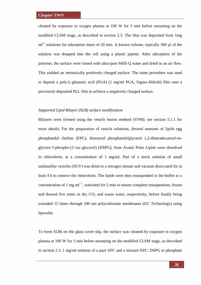
Chapter TWO
38
cleaned by exposure to oxygen plasma at 100 W for 3 min before mounting on the
modified CLSM stage, as described in section 2.3. The film was deposited from 1mg
ml-1
solutions for adsorption times of 20 min. A known volume, typically 500 µl of the
solution was dropped into the cell using a plastic pipette. After adsorption of the
polymer, the surface were rinsed with ultra-pure Milli-Q water and dried in an air flow.
This yielded an intrinsically positively charged surface. The same procedure was used
to deposit a poly-L-glutamic acid (PGA) (1 mg/ml PGA, Sigma-Aldrish) film onto a
previously deposited PLL film to achieve a negatively charged surface.
Supported Lipid Bilayer (SLB) surface modification
Bilayers were formed using the vesicle fusion method (VFM); see section 5.1.1 for
more details. For the preparation of vesicle solutions, desired amounts of lipids egg
phosphatidyl choline (EPC); distearoyl phosphatidylglycerol 1,2-ditetradecanoyl-sn-
glycero-3-phospho-(1'-rac-glycerol) (DSPG); from Avanti Polar Lipids were dissolved
in chloroform, at a concentration of 1 mg/ml. Part of a stock solution of small
unilamellar vesicles (SUV) was dried in a nitrogen stream and vacuum desiccated for at
least 4 h to remove the chloroform. The lipids were then resuspended in the buffer to a
concentration of 1 mg ml−1
, sonicated for 2 min to ensure complete resuspension, frozen
and thawed five times in dry CO2 and warm water, respectively, before finally being
extruded 15 times through 100 nm polycarbonate membranes (GC Technology) using
liposofat.
To form SLBs on the glass cover slip, the surface was cleaned by exposure to oxygen
plasma at 100 W for 3 min before mounting on the modified CLSM stage, as described
in section 2.3. 1 mg/ml solution of a pure EPC and a mixture EPC: DSPG in phosphate

Chapter TWO
39
buffer was prepared in two molar ratios 80:20 and 60:40. A known volume, typically
500 µl, of SUV solution was dropped into the cell using a plastic pipette containing
buffer solution. After allowing 128 minutes to elapse the resulting SLB was rinsed with
the buffer. The cell was filled gradually using a plastic pipette with 1 mL of the
solution to be used for imaging, typically consisting of 8 μM fluorescein and 0.1 M
potassium nitrate.
Monitoring SLB Formation
Bilayer formation was observed using ScanAsyst-atomic force microscopy (SA-AFM)
in real time, with assistance from Mr. Mike O'Connell and Mr. Binoy Nadappuram. The
glass cover slip (glass bottom dishes, WillCo-dish®KIT) were cleaned by exposure to
oxygen plasma at 100 W for 3 min. 500 μl of 1 mg ml−1
EPC-DSPG SUV solution was
pipetted into the buffer solution onto the glass microscope slides and kept under
solution for SA-AFM imaging. Topographical images of the surface were obtained
using a Veeco Bruker Bioscope Catalyst AFM typically at a resolution of 256 by 256
pixels at 2 Hz, using the different stiffness cantilevers of SNL-type silicon nitride
probes with nominal force constant, k, of 0.32 and 0.58 N m−1
, respectively, and a
resonant frequency, f 0, of 40−75 kHz.
2.2. Device Microfabrication and Characterisation
2.2.1. Pt Ultramicroelectrode (UME) Fabrication and Characterisation
The procedure used for UME fabrication was based on the method developed by
Wightman and Bard et al..1. A disk-shaped tip was made by heat sealing a 1.5 cm length
of 25 μm diameter metal microscopic wire (platinum) into a borosilicate glass capillary
tube (GC200-10, 2.0 mm inner diameter, 1.16 mm outer diameter, Harvard Apparatus

Chapter TWO
40
Ltd. Kent, U.K.). The end was then polished to expose an embedded disk. A coarse
carbimet paper disc (240 grit, Buehler, Coventry) was used to polish the tip of the glass
capillary to expose the end of the wire. A finer grade (600 grit, Buehler, Coventry) and
then waterproof silicon carbide paper (SIC Paper #4000, Struers) were used to smooth
the surface of the tip, to obtain a flat surface. Further polishing with impregnated
diamond polishing pads (Buehler, Coventry) of sequentially finer grades (from 9 μm to
0.1 μm) was carried out using a custom built polishing wheel.
Figure 2.1: Conventional light microscope image of the tip of a 25 μm diameter
platinum disc UME: (a) from the side; (b) the electrode surface.
An insulator radius of 10 times larger than the electrode radius (the RG ratio) is usually
desirable.2 The sides of the electrode were ‘coned’ (polished) using waterproof silicon
carbide paper to give the electrode the required RG value. Optical microscope images
of UMEs obtained in this way are given in Figure 2.1. Silver loaded epoxy adhesive
(RS) was used to coat the end of a piece of tinned copper wire (RS), which was then
inserted into the capillary, ensuring that it was in contact with the Pt wire. This was left
to dry before testing the connection.
a) b)
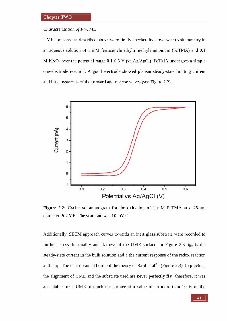
Chapter TWO
41
Characterisation of Pt-UME
UMEs prepared as described above were firstly checked by slow sweep voltammetry in
an aqueous solution of 1 mM ferrocenylmethyltrimethylammonium (FcTMA) and 0.1
M KNO3 over the potential range 0.1-0.5 V (vs Ag/AgCl). FcTMA undergoes a simple
one-electrode reaction. A good electrode showed plateau steady-state limiting current
and little hysteresis of the forward and reverse waves (see Figure 2.2).
Figure 2.2: Cyclic voltammogram for the oxidation of 1 mM FcTMA at a 25-μm
diameter Pt UME. The scan rate was 10 mV s-1
.
Additionally, SECM approach curves towards an inert glass substrate were recorded to
further assess the quality and flatness of the UME surface. In Figure 2.3, ilim is the
steady-state current in the bulk solution and it the current response of the redox reaction
at the tip. The data obtained bore out the theory of Bard et al2-3
(Figure 2.3). In practice,
the alignment of UME and the substrate used are never perfectly flat, therefore, it was
acceptable for a UME to touch the surface at a value of no more than 10 % of the

Chapter TWO
42
normalised current. Experimentally, when the UME touches a surface there was a point
of inflection, or plateau in the experimental curve as shown in Figure 2.3. Before each
set of measurements, the electrode was polished using slurry of alumina particles (0.05
μm gamma alumina Micropolish, Buehler, Coventry) in water on a polishing cloth to
ensure that the surface was clean and smooth.
Figure 2.3: SECM experimental approach curve (red line) and the theory (blue line)
towards inert glass substrate performed in 0.1 M KNO3.
2.2.2. Optically Transparent Single-Walled Carbon Nanotubes
Ultramicroelectrodes (OT-SWNTs- UMEs): Fabrication and
Characterisation
cCVD Growth of CNT networks
Carbon nanotube ultrathin mats were grown (by Dr. Agnieszka Rutkowska)4 directly on
single crystal quartz substrates (Hoffman Materials, Inc., 3 in. diameter, angle cut:
42°45′, 500 µm thick, double side polish) using catalysed chemical vapour deposition
technique (as illustrated in Figure 2.4). 1.2 cm x 1.2 cm quartz samples were cleaned
with acetone and isopropanol and blown dry with nitrogen, followed by sputter
Chapter TWO
43
depositing of a thin film of cobalt for 20 seconds (Quorum Technologies sputter coater).
The samples were placed on a quartz boat with a Si/SiO2 support on top (IDB
Technologies Ltd., 0.5 mm thick, n-type Si, 300 nm thermally grown SiO2) in the centre
of a 1 in. quartz tube of the cCVD oven (Lindberg Blue).5 The magnitude of the
hydrogen flow and the growth temperature were optimised by AFM examination of the
NP size. For the conditions stated above, a NP size of ~ 4-8 nm was found to be optimal
for SWNT growth. Methane was introduced at 875 °C for a period of time and the flow
rate adjusted so that the total flow rate of gases was kept at 2000 sccm.
Figure 2.4: Schematic illustration the procedure for growing single-walled carbon
nanotubes ultrathin mats using catalysed chemical vapour deposition technique.
The samples were heated from room temperature to 700 ºC within 10 min and up to 850
ºC within next 10 min in the presence of hydrogen flow (150 sccm). The system was
stabilized for 5 min and ethanol was supplied by introducing a flow of argon (850 sccm)
through an ethanol bubbler held at 0 ºC. The flow of argon was terminated after 10 min
and the system was allowed to cool down to room temperature under a hydrogen flow
(150 sccm).

Chapter TWO
44
Preparation of SWNTs-OT-UMEs
The gold contacts were evaporated onto SWNTs-functionalised quartz samples through
a shadow mask (Figure 2.5) using a Moorfield Minilab Conversion evaporator/sputterer
unit at a deposition rate of 0.05Å/s and 1.5 Å/s for chromium (Testbourne Ltd.) and
gold (Goodfellow), respectively. Chromium with a thickness of 10 nm was used as a
support layer to increase the adhesion of gold (thickness 120 nm) to the substrate. Disc
UMEs were prepared by UV photolithographical exposure using Suss mask aligner
(MJB4 mask aligner, Suss MicroTec, 4 seconds UV exposure time) and S1818 positive
photoresist (Rohm and Haas Electronic Materials) with an adhesive microprimer
support layer (Rohm and Haas Electronic Materials). The conditions for spin coating
substrates with primer and S1818 are listed in Table 2.1. Spin coating samples with
primer was followed by ca. 1.5 µm of primer + S1818 photoresist deposition. Samples
coated with S1818 were soft baked at 115 °C for 1 min to ensure good adhesion of the
layers to the substrate before the photolithographical step.
Table 2.1: Conditions for spin coating samples with microprime primer and S1818
positive photoresist.
Chemical
Rotation
Acceleration
time (s)
Spin
time (s)
speed
(rpm)
Deceleration
time (s)
Primer 0.1 40 3000 0.1
S1818 0.1 40 3000 0.1

Chapter TWO
45
Figure 2.5: (a) Schematic of the procedure used for fabricating SWNTs network disk
UMEs, (bi) Geometry of the shadow mask used for microfabrication of Cr/Au bands for
disk UME experiments, (bii) Photographs of CNT device used in electrochemical
experiments.
50µm disc electrodes were aligned to the geometry of the Au bands so that the edge of
the UME was at a sufficient distance away from the Cr/Au layer, ensuring it could not
compromise the pristine integrity. The pattern was developed by soaking in MF 319
developer solution (Rohm and Haas Electronic Materials) for 1 min, followed by rinsing
with Milli-Q water and blowing dry with nitrogen flow.
Characterisation of SWNTs network mat
Several techniques were employed throughout this thesis to investigate the results of
cCVD growth and to characterize the SWNTs networks and devices obtained. Details of
these techniques are given in this section. The transparency of SWNTs mats on ST-cut
quartz was measured using a standard UV-Vis spectrophotometer (Jasco V-660).
(a)
(bi) (bii)
Chapter TWO
46
Atomic Force Microscopy
Atomic force microscopy (AFM EnviroScopeTM, Veeco) was used to verify the
density of SWNTs films. AFM was conducted in tapping mode. The principle of
operation is based on a feedback loop, where the cantilever is brought to resonance and
is oscillated close to the sample so that the tip periodically touches the surface. This
imaging mode is used for soft samples, as lateral tip-surface forces are minimized. Most
importantly for the work herein is that it prevents dragging of SWNTs on the surface.
AFM tips employed (RFESP, Multi75 metrology probes, Veeco Probes, U.S.A.) had
resonant frequencies of 75-100 kHz and force constants of 1.5-6 N m-1
.
Micro-Raman Spectroscopy
Micro-Raman spectra of SWNTs networks were recorded using a Renishaw inVia
microscope incorporated with Leica microscope and CCD detector. SWNTs peaks were
calibrated against at 521 cm-1
. A 514.5 nm (2.41 eV energy) excitation wavelength of
an Ar laser, at 10 mW power, focused in a ~ 10 µm2 spot size, was used in the
experiments to determine the quality of the grown SWNTs and to confirm the presence
of uniform and defect-free SWNTs. Raman spectroscopy is a broadly used technique for
quantitative analysis of SWNTs structural and physical properties. The presence of
SWNTs was confirmed with micro-Raman spectroscopy (Figure 2.6) by characteristic
G+ (1594:5 cm
-1) and G
- (1576:6 cm
-1) peaks and the small distortion (D) peak at 1342:6
cm-1
.

Chapter TWO
47
Figure 2.6: Micro-Raman spectrum of SWNTs ultrathin mats grown on single crystal
quartz.
2.3. CLSM Experiments
Confocal fluorescence imaging was performed using a Leica TCS SP5X
Supercontinuum laser scanning confocal microscope mounted on a Leica DMI6000 CS
inverted microscope. Typically, the following parameters were used: 488 nm excitation
wavelength (Ar laser), detector window 480-570 nm, and 8000 Hz line scanning
frequency. Well-defined proton flux for high resolution time (ms) was achieved via a
built in-house galvanostat. A two electrode galvanosatic arrangement with Pt reference
electrode (Ag/AgCl RE), and an UME (25 μm diameter Pt disc, with a glass surround of
250 μm diameter, fabricated as described in section 2.1) as working electrode was used.
Anodic current was applied at the working electrode to produce a proton flux via water
oxidation and images of the resulting fluorescence profiles captured.
H2O 2H+ + ½ O2 + 2e
(2.1)

Chapter TWO
48
2.3.1. Visualisation of Electrochemical Processes at OT-SWNTs-UMEs
The experimental setup for simultaneous electrochemical (CompactStat, Ivium
Technologies) and fluorescence confocal imaging (Inverted Leica TCS SP5X
Supercontinuum Confocal) studies is shown schematically in Figure 2.7. The CNT
electrode device was placed on an aluminium sample holder (designed in house of size
of 7.5 cm x 2.5 cm x 0.5 cm) with 1 cm x 1 cm hole in the centre for CLSM imaging. A
drop of the solution of interest was cast on top of a 50 µm diameter OT-UME. Figure
2.5 illustrates the case for aqueous Ru(bpy)32+
of various concentrations: 1 mM, 5 mM
and 10 mM, in 0.1 M sodium chloride. The electrochemistry of redox reactions of
Ru(bpy)32+
and fluorescein were visualized using an inverted microscope (Leica
DMI6000 CS) in fluorescence mode, using 488 nm argon laser.
The gain and the offset of the channel were adjusted according to the experiment: (i)
low initial intensity below and at the electrode surface, (ii) high initial intensity at the
electrode surface and low below its plane, for fluorescein and Ru(bpy)32+
experiments,
respectively. The surface was defined prior to any electrochemical experiment by
scanning across the sample (in the z direction: xyz scan) in the bright field mode and
collecting z-stacks (z-volume = 150 μm, z-step = 2 μm) from below and above the
initially focused UME.

Chapter TWO
49
Figure 2.7: Schematic representation of the experimental setup used for visualising OT-
SWNTs-UMEs.
Cyclic voltammetry (CVs) of the redox couples was performed by cyclic sweep of the
potential in an appropriate range versus Ag/AgCl reference electrode at a scan rate of 10
mV/s and 5 mV/s for fluorescein and Ru(bpy)32+
, respectively. The process was
monitored (xyt scan, t = 180 s) with CLSM fluorescence and brightfield modes. To
synchronise the light intensity measured by CLSM and the potential applied, the CLSM
was triggered by the potentiostat (Leica Trigger Unit connected with the Ivium
CompactStat by DAQPad-6015, National Instruments). This enabled the CLSM light
intensity signal adjacent to the electrode plane to be related to the potential change
driving the redox reaction.
The choice of the microscope objectives was limited to 10x magnification and 0.3
aperture and 11.0 mm free working distance (HC PL FLUOTAR type for DRY
Aluminium
sample holder
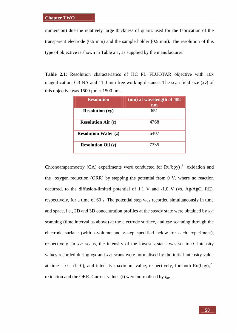
Chapter TWO
50
immersion) due the relatively large thickness of quartz used for the fabrication of the
transparent electrode (0.5 mm) and the sample holder (0.5 mm). The resolution of this
type of objective is shown in Table 2.1, as supplied by the manufacturer.
Table 2.1: Resolution characteristics of HC PL FLUOTAR objective with 10x
magnification, 0.3 NA and 11.0 mm free working distance. The scan field size (xy) of
this objective was 1500 µm × 1500 µm.
Resolution (nm) at wavelength of 488
nm
Resolution (xy) 651
Resolution Air (z) 4768
Resolution Water (z) 6407
Resolution Oil (z) 7335
Chronoampermoetry (CA) experiments were conducted for Ru(bpy)32+
oxidation and
the oxygen reduction (ORR) by stepping the potential from 0 V, where no reaction
occurred, to the diffusion-limited potential of 1.1 V and -1.0 V (vs. Ag/AgCl RE),
respectively, for a time of 60 s. The potential step was recorded simultaneously in time
and space, i.e., 2D and 3D concentration profiles at the steady state were obtained by xyt
scanning (time interval as above) at the electrode surface, and xyz scanning through the
electrode surface (with z-volume and z-step specified below for each experiment),
respectively. In xyz scans, the intensity of the lowest z-stack was set to 0. Intensity
values recorded during xyt and xyz scans were normalised by the initial intensity value
at time = 0 s (It=0), and intensity maximum value, respectively, for both Ru(bpy)32+
oxidation and the ORR. Current values (i) were normalised by ilim.
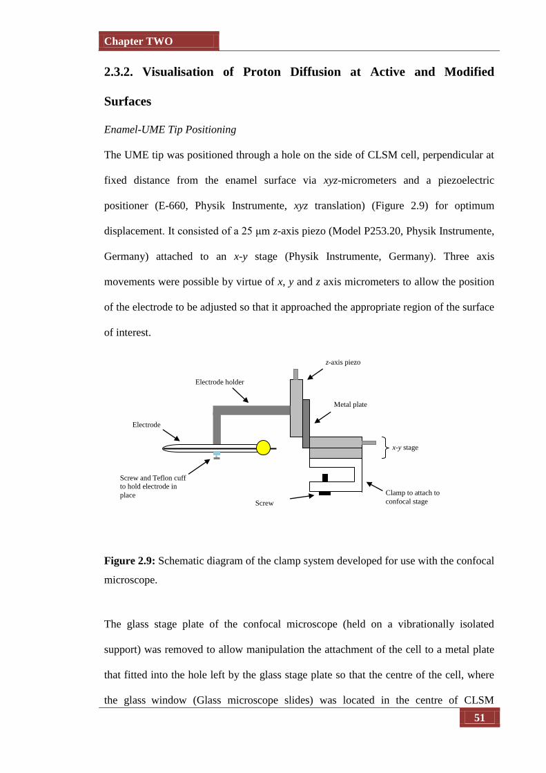
Chapter TWO
51
2.3.2. Visualisation of Proton Diffusion at Active and Modified
Surfaces
Enamel-UME Tip Positioning
The UME tip was positioned through a hole on the side of CLSM cell, perpendicular at
fixed distance from the enamel surface via xyz-micrometers and a piezoelectric
positioner (E-660, Physik Instrumente, xyz translation) (Figure 2.9) for optimum
displacement. It consisted of a 25 μm z-axis piezo (Model P253.20, Physik Instrumente,
Germany) attached to an x-y stage (Physik Instrumente, Germany). Three axis
movements were possible by virtue of x, y and z axis micrometers to allow the position
of the electrode to be adjusted so that it approached the appropriate region of the surface
of interest.
Figure 2.9: Schematic diagram of the clamp system developed for use with the confocal
microscope.
The glass stage plate of the confocal microscope (held on a vibrationally isolated
support) was removed to allow manipulation the attachment of the cell to a metal plate
that fitted into the hole left by the glass stage plate so that the centre of the cell, where
the glass window (Glass microscope slides) was located in the centre of CLSM
Screw
Screw and Teflon cuff to hold electrode in
place
Electrode
Electrode holder
z-axis piezo
Metal plate
x-y stage
Clamp to attach to
confocal stage
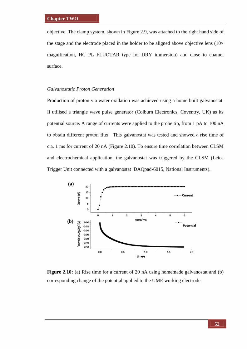
Chapter TWO
52
objective. The clamp system, shown in Figure 2.9, was attached to the right hand side of
the stage and the electrode placed in the holder to be aligned above objective lens (10×
magnification, HC PL FLUOTAR type for DRY immersion) and close to enamel
surface.
Galvanostatic Proton Generation
Production of proton via water oxidation was achieved using a home built galvanostat.
Ii utilised a triangle wave pulse generator (Colburn Electronics, Coventry, UK) as its
potential source. A range of currents were applied to the probe tip, from 1 pA to 100 nA
to obtain different proton flux. This galvanostat was tested and showed a rise time of
c.a. 1 ms for current of 20 nA (Figure 2.10). To ensure time correlation between CLSM
and electrochemical application, the galvanostat was triggered by the CLSM (Leica
Trigger Unit connected with a galvanostat DAQpad-6015, National Instruments).
Figure 2.10: (a) Rise time for a current of 20 nA using homemade galvanostat and (b)
corresponding change of the potential applied to the UME working electrode.
(a)
(b)
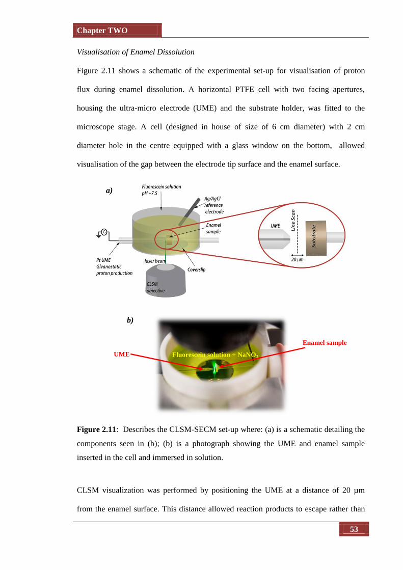
Chapter TWO
53
Visualisation of Enamel Dissolution
Figure 2.11 shows a schematic of the experimental set-up for visualisation of proton
flux during enamel dissolution. A horizontal PTFE cell with two facing apertures,
housing the ultra-micro electrode (UME) and the substrate holder, was fitted to the
microscope stage. A cell (designed in house of size of 6 cm diameter) with 2 cm
diameter hole in the centre equipped with a glass window on the bottom, allowed
visualisation of the gap between the electrode tip surface and the enamel surface.
Figure 2.11: Describes the CLSM-SECM set-up where: (a) is a schematic detailing the
components seen in (b); (b) is a photograph showing the UME and enamel sample
inserted in the cell and immersed in solution.
CLSM visualization was performed by positioning the UME at a distance of 20 µm
from the enamel surface. This distance allowed reaction products to escape rather than
Fluorescein solution + NaNO3
Enamel sample
UME
b)
a)
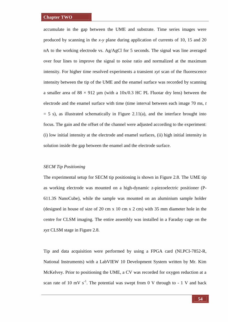
Chapter TWO
54
accumulate in the gap between the UME and substrate. Time series images were
produced by scanning in the x-y plane during application of currents of 10, 15 and 20
nA to the working electrode vs. Ag/AgCl for 5 seconds. The signal was line averaged
over four lines to improve the signal to noise ratio and normalized at the maximum
intensity. For higher time resolved experiments a transient xyt scan of the fluorescence
intensity between the tip of the UME and the enamel surface was recorded by scanning
a smaller area of 88 × 912 µm (with a 10x/0.3 HC PL Fluotar dry lens) between the
electrode and the enamel surface with time (time interval between each image 70 ms, t
= 5 s), as illustrated schematically in Figure 2.11(a), and the interface brought into
focus. The gain and the offset of the channel were adjusted according to the experiment:
(i) low initial intensity at the electrode and enamel surfaces, (ii) high initial intensity in
solution inside the gap between the enamel and the electrode surface.
SECM Tip Positioning
The experimental setup for SECM tip positioning is shown in Figure 2.8. The UME tip
as working electrode was mounted on a high-dynamic z-piezoelectric positioner (P-
611.3S NanoCube), while the sample was mounted on an aluminium sample holder
(designed in house of size of 20 cm x 10 cm x 2 cm) with 35 mm diameter hole in the
centre for CLSM imaging. The entire assembly was installed in a Faraday cage on the
xyz CLSM stage in Figure 2.8.
Tip and data acquisition were performed by using a FPGA card (NI.PCI-7852-R,
National Instruments) with a LabVIEW 10 Development System written by Mr. Kim
McKelvey. Prior to positioning the UME, a CV was recorded for oxygen reduction at a
scan rate of 10 mV s-1
. The potential was swept from 0 V through to - 1 V and back
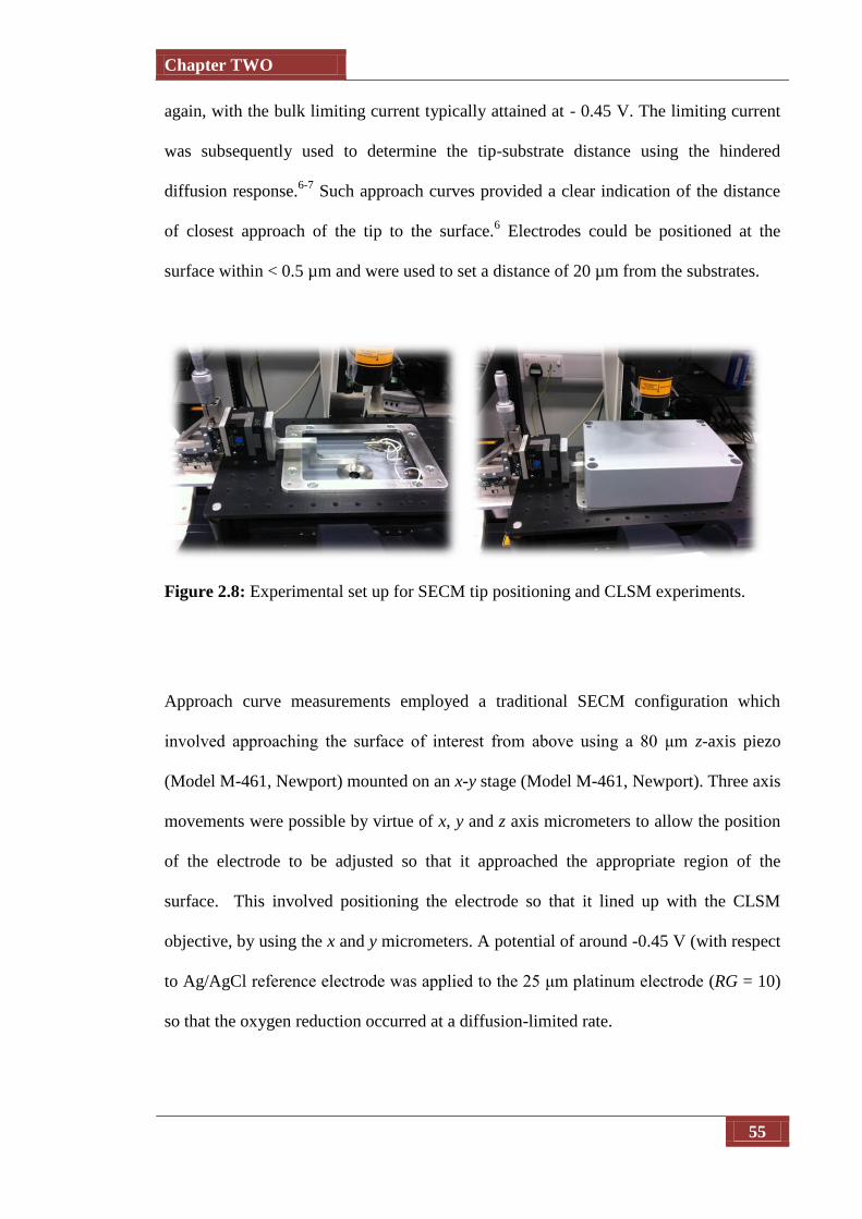
Chapter TWO
55
again, with the bulk limiting current typically attained at - 0.45 V. The limiting current
was subsequently used to determine the tip-substrate distance using the hindered
diffusion response.6-7
Such approach curves provided a clear indication of the distance
of closest approach of the tip to the surface.6 Electrodes could be positioned at the
surface within < 0.5 µm and were used to set a distance of 20 µm from the substrates.
Figure 2.8: Experimental set up for SECM tip positioning and CLSM experiments.
Approach curve measurements employed a traditional SECM configuration which
involved approaching the surface of interest from above using a 80 μm z-axis piezo
(Model M-461, Newport) mounted on an x-y stage (Model M-461, Newport). Three axis
movements were possible by virtue of x, y and z axis micrometers to allow the position
of the electrode to be adjusted so that it approached the appropriate region of the
surface. This involved positioning the electrode so that it lined up with the CLSM
objective, by using the x and y micrometers. A potential of around -0.45 V (with respect
to Ag/AgCl reference electrode was applied to the 25 μm platinum electrode (RG = 10)
so that the oxygen reduction occurred at a diffusion-limited rate.
Chapter TWO
56
The electrode was then brought closer to the surface using the z micrometer. The
current, monitored by a current follower system coupled to a triangular wave-pulse
generator with a voltmeter displaying the current output, began to change when the
electrode was within a distance of about 10 electrode radii from the substrate.3
Approach curves for oxygen reduction (while the electrode was held a -0.45 V with
respect to a silver/silver chloride reference electrode (Ag/AgCl RE) in fluorescein
solution were obtained. Once the current was seen to alter, the z-axis piezo was used so
that the distance moved by the electrode was accurately known. Once the tip-substrate
distance had been set, the working electrode was connected to the galvanostat.
Visualization of Lateral Proton Diffusion at Modified Surfaces
A small dish (50 x 9 mm, WillCo-dishes) was used as the experimental cell with glass
windows at the bottom of the dishes (0.15 or 0.17 mm thick). This was simply fixed to
the microscope stage. The major advantage of this glass bottom is that the microscope
light passes orthogonally through the glass bottom and there is no air-buffer between the
warming-stage and the glass, which could seriously disrupt efforts to regulate the
temperature of the cells in the dish.
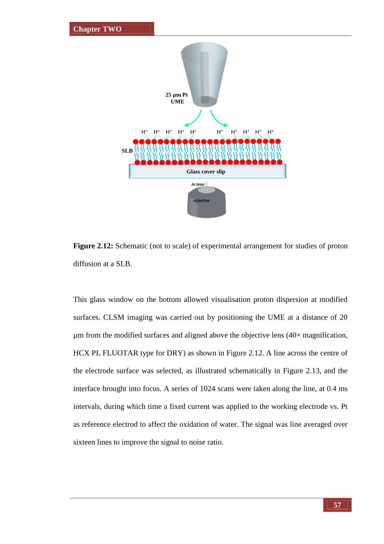
Chapter TWO
57
Figure 2.12: Schematic (not to scale) of experimental arrangement for studies of proton
diffusion at a SLB.
This glass window on the bottom allowed visualisation proton dispersion at modified
surfaces. CLSM imaging was carried out by positioning the UME at a distance of 20
µm from the modified surfaces and aligned above the objective lens (40× magnification,
HCX PL FLUOTAR type for DRY) as shown in Figure 2.12. A line across the centre of
the electrode surface was selected, as illustrated schematically in Figure 2.13, and the
interface brought into focus. A series of 1024 scans were taken along the line, at 0.4 ms
intervals, during which time a fixed current was applied to the working electrode vs. Pt
as reference electrod to affect the oxidation of water. The signal was line averaged over
sixteen lines to improve the signal to noise ratio.
H+ H+ H+ H+ H+H+H+H+H+H+
25 µm Pt
UME
Glass cover slip
SLB

Chapter TWO
58
Figure 2.13: Schematic of experimental arrangement for studies of proton diffusion in a
thin layer.
2.4 Additional Instrumentation
2.4.1. Inductively Coupled Plasma Mass Spectrometry (ICP-MS)
Experiments were performed by Dr. Lijiang Song, using ICP-MS (PerkinElmer
5300DV, equipped with S10 Autosampler) to determine the amount of zinc taken up by
enamel treatment discussed in section 2.1. ICP was calibrated with ZnCl2 solution 500
ppb, 200 ppb, 100ppb, 50 ppb, 20 ppb and 10 ppb. As the enamel discs have a diameter
of 6.76 mm (equivalent to an area of 0.457 cm2) a volume of 0.1 ml was chosen as this
droplet covered the entire area of the sample without running off. The droplet was then
pipetted off and diluted in 5ml for analysis.
25 µm Pt
UME
Line scanned across
the UME
Glass cover slip

Chapter TWO
59
2.4.2. Fluoride Ion Selective Electrode (FISE) Studies
To determine the amount of fluoride taken up by enamel, experiments were performed
by Dr. Carrie-Anne McGeouch, using a solid state FISE (model ELIT 001N AgCl
58997), the working electrode (model Elit F- 1230), and the reference electrode was
Ag/AgCl. Samples to be analysed were treated with either 500 or 1000 ppm of NaF
(0.026 and 0.053 molar equivalent) for two minutes then dissolved using 0.1 ml of 1
mM HNO3, also for two minutes. The droplet was then pipetted off for FISE analysis.
For calibration, a 0.1 M solution of NaF was prepared and subsequently diluted to give
concentrations of 10-2
, 10-3
and 10-4
M.
2.5. Finite Element Modelling
Modeling was carried out using a commercial finite element method modelling package
(COMSOL Multiphysics, version 3.2a), in conjunction with MATLABm (version 7.0,
release 14). This was run on a Dell PC under Windows XP with an Intel Pentium 4
processor (2.50 GHz) and 1.5 GB of RAM.
2.6. Solution Preparation
All solutions were prepared using Milli-Q water (Millipore Corp, resistivity ≥ 18 MΩ
cm), with the mass of material added determined with a four-figure analytical balance
(Sartorius A2008). pH measurements were made using a pH meter (UltraBasic pH
Meter, Denver Instruments), calibrated using buffer solutions at pH 4, 7 and 10
(“colourkey” buffer solutions, BDH).
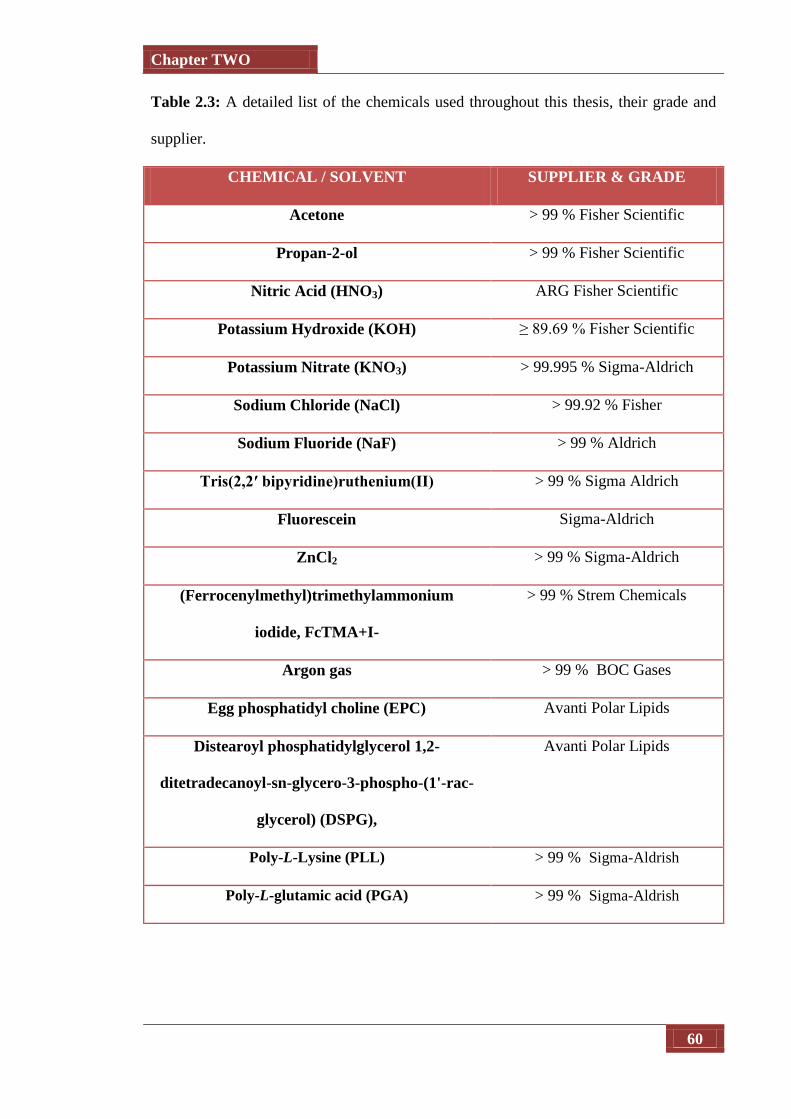
Chapter TWO
60
Table 2.3: A detailed list of the chemicals used throughout this thesis, their grade and
supplier.
CHEMICAL / SOLVENT SUPPLIER & GRADE
Acetone > 99 % Fisher Scientific
Propan-2-ol > 99 % Fisher Scientific
Nitric Acid (HNO3) ARG Fisher Scientific
Potassium Hydroxide (KOH) ≥ 89.69 % Fisher Scientific
Potassium Nitrate (KNO3) > 99.995 % Sigma-Aldrich
Sodium Chloride (NaCl) > 99.92 % Fisher
Sodium Fluoride (NaF) > 99 % Aldrich
Tris(2,2′ bipyridine)ruthenium(II) > 99 % Sigma Aldrich
Fluorescein Sigma-Aldrich
ZnCl2 > 99 % Sigma-Aldrich
(Ferrocenylmethyl)trimethylammonium
iodide, FcTMA+I-
> 99 % Strem Chemicals
Argon gas > 99 % BOC Gases
Egg phosphatidyl choline (EPC) Avanti Polar Lipids
Distearoyl phosphatidylglycerol 1,2-
ditetradecanoyl-sn-glycero-3-phospho-(1'-rac-
glycerol) (DSPG),
Avanti Polar Lipids
Poly-L-Lysine (PLL) > 99 % Sigma-Aldrish
Poly-L-glutamic acid (PGA) > 99 % Sigma-Aldrish

Chapter TWO
61
2.7. References
(1) Demaille, C.; Brust, M.; Tsionsky, M.; Bard, A. J. Analytical Chemistry 1997, 69,
2323.
(2) Bard, A. J.; Fan, F. R. F.; Kwak, J.; Lev, O. Analytical Chemistry 1989, 61, 132.
(3) Kwak, J.; Bard, A. J. Analytical Chemistry 1989, 61, 1221.
(4) Rutkowska, A.; Bawazeer, T. M.; Macpherson, J. V.; Unwin, P. R. Physical
Chemistry Chemical Physics 2011, 13, 5223.
(5) Rutkowska, A.; Walker, D.; Gorfman, S.; Thomas, P. A.; Macpherson, J. V.
Journal of Physical Chemistry C 2009, 113, 17087.
(6) Kwak, J.; Bard, A. J. Anal. Chem. 1989, 61, 1221.
(7) Gonsalves, M.; Barker, A. L.; Macpherson, J. V.; Unwin, P. R.; O'Hare, D.;
Winlove, C. Biophys. J. 2000, 1578.

Chapter THREE
62
Visualisation of Electrochemical Processes at Optically
Transparent Single-Walled Carbon Nanotube
Ultramicroelectrodes
(OT-SWNTs-UME)
3
Introduction
This chapter concerns the investigation of mass transport in microscale systems. A
major focus is on Confocal Laser Scanning Microscopy (CLSM) as a means of
visualising diffusion and reactions of fluorescently active species at optically
transparent ultramicroelectrodes (OP-UMEs) comprising Carbon Nanotube (CNT)
networks on quartz. The electrochemical activity of the UMEs is quantified with the
temporal and spatial resolution in the millisecond and micrometer range, respectively.
The methodology comprises of tracking the dynamic, reversible concentration profiles
of electroactive and photoactive tris(2,2'-bipyridine)ruthenium(II) species in aqueous
solutions during cyclic voltammetry experiments. Specifically a decrease of
fluorescence intensity is recorded at and around the UME surface during the oxidation
of luminescent Ru(bpy)32+
to non-luminescent Ru(bpy)33+
, followed by an increase of
the intensity signal in the reverse scan direction as the oxidized Ru(bpy)33+
is consumed
at the electrode surface. A three dimensional map of the concentration gradients of
Ru(bpy)32+
is constructed by collecting sections of the object across the normal to the
electrode plane in the steady state current regime. This configuration enables optical
measurements of the solution, close to the electrode surface, without significant
interference from absorption or scattering processes.
3.1. Overview
Probing concentration profiles at electrode surfaces and other interfaces finds
applications in many interfacial processes. A wide range of processes in biology
(cellular and bacterial chemotaxis and synaptic transmission)1-2
and chemistry (phase-
transfer reactions,3-4
corrosion,5 crystal growth/dissolution and faradic currents)
6 are
controlled by mass transport and thus by the concentration gradient7-8
Consequently, a
variety of analytical methods have been devised to monitor the development of such
concentration profiles near an active surface. Visualisation of concentration gradients
Chapter THREE
63
near electrode surfaces is of interest as it provides details on the reaction mechanism, as
well as the electrode activity and sensitivity to certain species involved in
electrochemical processes.9
The current response at the electrode gives information on the concentration gradient
directly adjacent to it, but complete concentration profiles over the whole diffusion
layer give much more information. Because of this, much research, involving many
different techniques, has been carried out into imaging various interfacial processes.
The majority of reported approaches are devoted to adapting scanning electrochemical
microscopy techniques10-11
and the use of optical methods such as laser beam
deflection,12
absorption spectroscopy 13-14
(UV-Vis, X ray, IR, EPR, Raman)15-17
,
fluorescence microscopy18-21
and scanning optical techniques (fluorescence confocal
laser scanning microscopy8,22
and confocal resonance Raman microspectroscopy16-17,23
)
to image concentration gradients at active surfaces.
Among the electrochemical techniques that have been used to investigate concentration
profiles, both potentiometric and amperometric probes have been used at various
interfaces.1,24-28
For example potentiometric probes have been used to map the variation
in the Nernst potential across diffusion layers.25
In this study a 250 μm diameter
platinum electrode was held at a fixed potential, chosen such that it induced the
electrode reaction at a diffusion-limited rate, and the potential variation at a 5 μm
diameter disc UME were measured as it approached the larger electrode. By applying
the Nernst Equation, the concentration of the reactant and product (related by mass
balance), assuming their diffusion coefficients are the same, were determined.
Potentiometric probes also have been used by Amatore et al.25
to determine the
Chapter THREE
64
concentration profile of ferrocyanide/ferricyanide and the tetracyanoquinodimethane
(TCNQ) reduction reaction. However, despite their accuracy, potentiometric
measurements usually can be performed only under equilibrium conditions preventing
transient measurements.
Engstrom et al.27-28
first demonstrated that an UME amperometry set up could be used
to map concentration profiles adjacent to a large active surface, with micrometer spatial
resolution, and millisecond time resolution. Using this method the concentration profile
for intermediates of coupled solution reactions were obtained by altering the tip
potential. Amperometric tips are generally preferred since absolute concentrations are
obtained, instead of ratios of one species to another which are obtained with
potentiometry. A similar concept has been used by Amatore et al.26
to obtain transient
concentration profiles of the same systems that had been studied potentiometrically
(ferrocyanide/ferricyanide and the TCNQ reduction reaction).
Various studies have been carried out using scanning electrochemical microscopy
(SECM) to determine many interfacial processes. Bard et al.29
were the first to
investigate sample surfaces with SECM. Unwin and co-workers used SECM
extensively to directly observe reactions occurring at liquid/liquid, solid/liquid and
liquid/gas interfaces.4,30-33
All these electrochemical methods are very powerful as they
provide spatial and temporal resolutions in the micrometer and millisecond range
respectively, depending on the size of probe and technique used. SECM was reviewed
in Chapter 1 section 1.3.6.

Chapter THREE
65
The combination of microscopic and spectroscopic techniques with electrochemical
methods would constitute a very useful tool to investigate in situ the composition of the
electrochemical diffusion layers. Various studies have been carried out using the
absorption of electrogenerated species, as absorbance is directly proportional to
concentration (Beer-Lambert law). Spectroelectrochemical techniques have been used
to monitor multiple species, particularly if they absorb at different wavelength. This
method provides better selectivity, sensitivity and resolution than those techniques
involving refractive index measurement, allowing much more precise measurement of
the concentration profile.34
Spatially resolved spectroelectrochemistry has been used by
McCreery and co-workers to investigate homogeneous electron transfer reactions with
spatial resolution of less than 5 μm.35
Raman spectroscopy has also been used in order to examine concentration profiles as it
allows precise chemical characterisation of the species present during an
electrochemical reaction.16-17
As the focal plane of the microscope is altered, the
concentration at different distances from the electrode can be obtained since the
intensity of the Raman signal is proportional to the concentration of the species.
Confocal Raman microscopy allows more precise optical sectioning through a sample
since only Raman spectra originating from the illuminated point in the sample plane of
interest are detected. Thus, the out-of-focus contribution to the spectrum is minimised.
Amatore et al. have used confocal resonance Raman microscopy to image the
composition of a diffusion layer, focussed on investigating the effect of
conproportionation reactions.16-17,23
Chapter THREE
66
Another method that has been used to map electrochemical activity is luminescence
imaging.36-37
With this technique the light emitted from a fluorescence reaction or
electrogenerated chemiluminescence (ECL) is imaged. Engstrom and co-worker have
extensively used this technique to visualize various interfacial processes. In ECL
imaging, electrochemistry is used to generate a species at the electrode which reacts to
produce light emitting species such as Ru(bpy)32+
in the presence of C2O2-. The ECL
technique has been used to provide an image of the current density, illustrating the edge
effect of highly oriented pyrolytic graphite (HOPG),36-37
which was thought to be
electrochemically active only on the edge12
, and locating sites of activity differences on
composite electrodes.36-37
However, there is a limited number of species that undergo
electrochemiluminescence. Furthermore, the widespread application of this method is
restricted by the complexity of some ECL reaction sequences.18,20
The use of fluorescence based methods as an alternative to ECL is most suitable as there
are a wide range of substances that are themselves fluorescent or can react with an
electrochemically-produced species to produce fluorescent molecules.20
In
electrochemistry,9,19-21
so various attempts have used this process to establish
concentration gradients (pH gradients). Besides, there are numerous reagents whose
fluorescence is pH-dependent, such as quinine or Oregon green,38
but the most common
fluorescent acid-base indicator is fluorescein. It strongly emits at a wavelength of
approximately 515 nm in basic solution, when it is excited at 470 nm. Engstrom et al.
have applied the fluorescence technique to study different systems, including cathodic
centers in Al/Cu corrosion cells,18
local differences in the kinetics of composite
electrodes,19
and electrode activity for oxygen O2 evolution.18
Later, it was shown by
Amatore2 and co-workers, that real-time remote fluorescence imaging of two-

Chapter THREE
67
dimensional concentration profiles of Ru(II) reagent could be achieved using a
multichannel fibre bundle. Recently, the fluorescence technique has been combined
with SECM in order to observe the activity of a single molecule of enzyme adenosine
triphosphate (ATP) synthase, which was labelled with a pH sensitive fluorophore,
activated by the pH gradient across a membrane.12
Nevertheless, compared to conventional fluorescence microscopy, CLSM is superior in
terms of image contrast, signal-to-noise ratio and spatial resolution. The use of
fluorescence CLSM to monitor the concentration profile at an electrode surface during
an electrochemical reaction was successfully introduced by Unwin7-8,22
and co-workers.
CLSM was used to image 3D pH gradients at and near to an electrode surface. The
reduction of benzoquinone in unbuffered solution produced a local pH increase that
caused fluorescein to become deprotonated and hence fluoresce. This technique has
been used to image the diffusion field at UMEs of various geometries, so providing
information on local mass transfer.7,22
In particular, the technique has been used to
visualise proton gradients at an electrode during water oxidation and reduction.7,22
In
order to obtain quantitative data from the fluorescence CLSM images, the finite element
method has been used to simulate mass transport. Fluorescence microscopy had been
used previously to identify active sites on a variety of electrode surfaces,9,19-20
but
without the advantage of z-axis scanning through the solution, normal to the electrode
surface.
More recent works have been reported by Unwin8 and co-workers for quantitative
measurements of permeation through model biological membranes by using a
combination of laser confocal microscopy (CLSM) and micro-electrochemistry. The

Chapter THREE
68
technique uses an ultramicroelectrode (UME) placed close to one side of the membrane
boundary (roughly 20 microns away) to generate protons in the presence of weak acids
anions and a trace amount of fluorescein (pH-sensitive fluorophore). The generation of
protons by galvanostatic water oxidation reduced the local solution pH and thus
produced a dark domain, which could be imaged using CLSM. This approach was
supported by finite element modelling (FEM) to report the trend of decreasing
permeation coefficient as the weak acid molecules increase in size.8
Fluorescein, a widely used fluorophore, exhibits a pH-sensitive fluorescence signal. In
acidic media the fluorescence is weak, but as the pH rises the intensity of the
fluorescence increases (Figure 1.3). By altering the pH electrochemically, the
corresponding changes in light intensity provide information on pH gradients and
diffusion close to the electrode surface. A simple way to locally change the pH in an
aqueous solution is by oxidising or reducing the water to produce protons or hydroxide
ions, respectively, as shown in Equations 3.1 and 3.2.
H2O 2H+ + ½ O2 + 2e
2H2O + 2e H2 + 2OH
(3.1)
(3.2)
or by reducing dissolved oxygen, Equation 3.3 summarises the reaction in acidic
medium.39
O2 + 2H+ + 2e
H2O2
H2O2 + 2H+ + 2e
2H2O
(3.3)
(3.4)
These redox reactions can be driven by applying the appropriate potential or current to
the working electrode with respect to a reference and/or counter electrode. This reaction
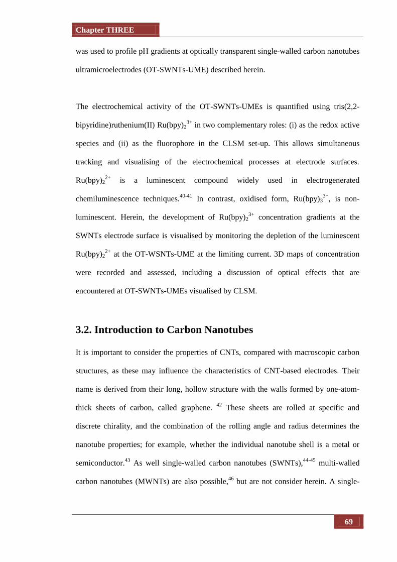
Chapter THREE
69
was used to profile pH gradients at optically transparent single-walled carbon nanotubes
ultramicroelectrodes (OT-SWNTs-UME) described herein.
The electrochemical activity of the OT-SWNTs-UMEs is quantified using tris(2,2-
bipyridine)ruthenium(II) Ru(bpy)23+
in two complementary roles: (i) as the redox active
species and (ii) as the fluorophore in the CLSM set-up. This allows simultaneous
tracking and visualising of the electrochemical processes at electrode surfaces.
Ru(bpy)22+
is a luminescent compound widely used in electrogenerated
chemiluminescence techniques.40-41
In contrast, oxidised form, Ru(bpy)33+
, is non-
luminescent. Herein, the development of Ru(bpy)23+
concentration gradients at the
SWNTs electrode surface is visualised by monitoring the depletion of the luminescent
Ru(bpy)22+
at the OT-WSNTs-UME at the limiting current. 3D maps of concentration
were recorded and assessed, including a discussion of optical effects that are
encountered at OT-SWNTs-UMEs visualised by CLSM.
3.2. Introduction to Carbon Nanotubes
It is important to consider the properties of CNTs, compared with macroscopic carbon
structures, as these may influence the characteristics of CNT-based electrodes. Their
name is derived from their long, hollow structure with the walls formed by one-atom-
thick sheets of carbon, called graphene. 42
These sheets are rolled at specific and
discrete chirality, and the combination of the rolling angle and radius determines the
nanotube properties; for example, whether the individual nanotube shell is a metal or
semiconductor.43
As well single-walled carbon nanotubes (SWNTs),44-45
multi-walled
carbon nanotubes (MWNTs) are also possible,46
but are not consider herein. A single-

Chapter THREE
70
walled carbon nanotube can be described as a one-atom-thick layer of graphite sheet
called graphene, rolled into a hollow seamless cylinder.45
Various techniques have been reported for nanotube growth, among which the most
developed and widely used are: arc discharge, laser ablation, chemical vapour
deposition (CVD) and high pressure carbon monoxide process based on the floating
CVD approach.47-49
This latter process is used for the bulk production of high-purity
SWNTs by Unidym Inc., U.S.A. Random networks of SWNTs can be grown by
catalysed chemical vapour deposition (cCVD) on silicon (Si) substrates50
and silicon
with an amorphous layer of silicon oxide (Si/SiO2)43,51-53
. An image of such a network,
as used in the work herein, is shown in Figure 3.1, obtained by field emission scanning
electron microscopy (FE-SEM).43
In cCVD synthesis, an iron, nickel or cobalt catalyst
(in the form of nanoparticles (NPs), whose size controls the diameter of the resulting
SWNT54
is placed on the substrate in an oven at 900 to 1000 °C. The carbon vapour
source absorbs into the catalyst NPs, causing it to form a liquid eutectic (metal carbide
55-56). Supersaturation of the catalyst results in solid precipitation forming SWNTs. If
synthesised in this way, the SWNTs require no further purification.
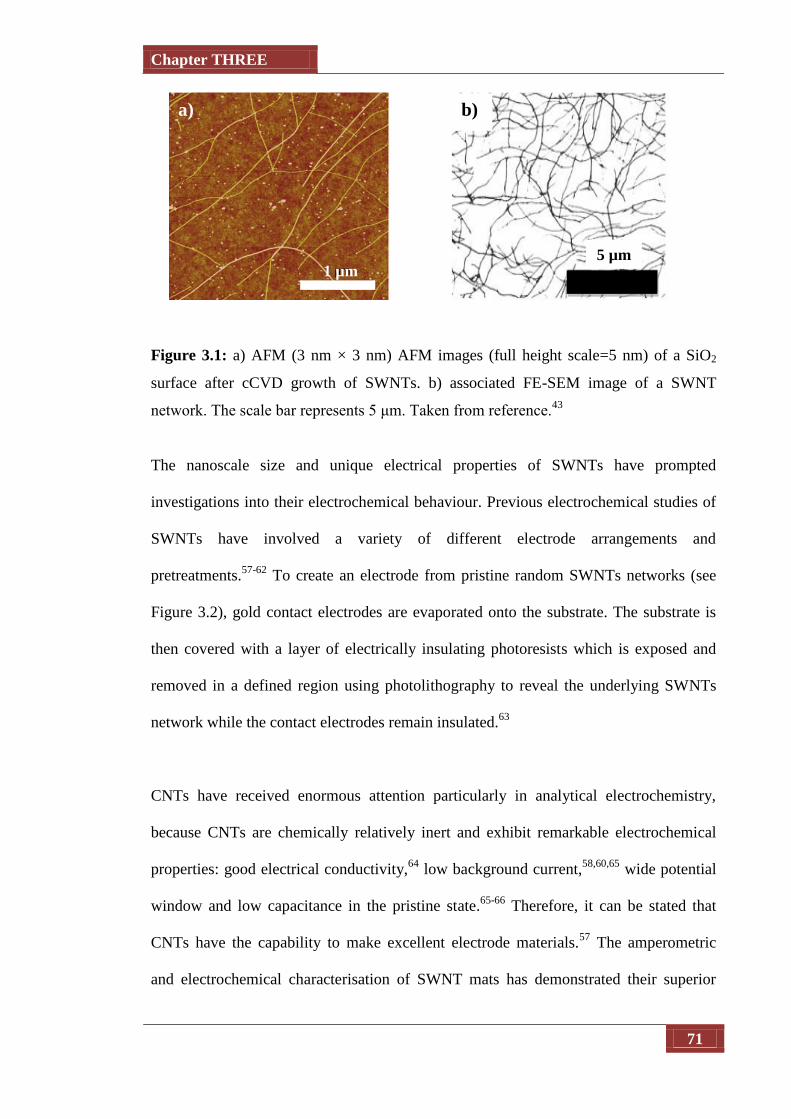
Chapter THREE
71
Figure 3.1: a) AFM (3 nm × 3 nm) AFM images (full height scale=5 nm) of a SiO2
surface after cCVD growth of SWNTs. b) associated FE-SEM image of a SWNT
network. The scale bar represents 5 μm. Taken from reference.43
The nanoscale size and unique electrical properties of SWNTs have prompted
investigations into their electrochemical behaviour. Previous electrochemical studies of
SWNTs have involved a variety of different electrode arrangements and
pretreatments.57-62
To create an electrode from pristine random SWNTs networks (see
Figure 3.2), gold contact electrodes are evaporated onto the substrate. The substrate is
then covered with a layer of electrically insulating photoresists which is exposed and
removed in a defined region using photolithography to reveal the underlying SWNTs
network while the contact electrodes remain insulated.63
CNTs have received enormous attention particularly in analytical electrochemistry,
because CNTs are chemically relatively inert and exhibit remarkable electrochemical
properties: good electrical conductivity,64
low background current,58,60,65
wide potential
window and low capacitance in the pristine state.65-66
Therefore, it can be stated that
CNTs have the capability to make excellent electrode materials.57
The amperometric
and electrochemical characterisation of SWNT mats has demonstrated their superior
1 µm 5 µm
b) a)
Chapter THREE
72
behaviour as disc UMEs, allowing applications in electroanalysis at concentrations well
below the capabilities of other carbon electrodes (e.g., GC). These features made them
very attractive electrode materials of high sensitivity. These SWNTs mats exhibit
absolute transparencies in the UV-Vis range.57
Optically transparent electrodes (OTEs) currently have widespread application in
modern electro-optical devices,67-68
such as solar cells69
, liquid crystal displays (LCDs),
thin film transistors (TFTs) or light-emitting diodes (LEDs), and are typically based on
thin layers of indium-tin-oxide (ITO).67
Although ITO exhibits high electrical
conductivity, it has some limitation as it is considered a brittle, rough and costly
material.69-70
Alternatively, a wide range of OTEs have been introduced based on the
deposition of other transparent conductive thin films. The most attractive among them
are films of carbon nanostructures, However, designing a film-based OTE requires a
thickness of typically tens of nanometers,71
to be optically transparent. At such
thickness, most electrode materials exhibit large internal resistances. So, there is a
tradeoff between optical transparency and electrical resistivity when designing OTEs.72
SWNTs exhibit superior flexibility in terms of conductivity and transparency, and have
been successfully used as optically transparent flexible TFTs, solar cells, and in
spectroelectrochemistry.73
Herein, the use of SWNTs mats are introduced as optically transparent UMEs by using
single crystal quartz as a substrate and visualizing the electrochemical processes at the
UME surface (from the back) with state-of-the-art fluorescence CLSM. The work
herein, as well as demonstrating attractive opto-electrochemical properties of SWNTs
electrodes, provides a platform for the extensive development and application of CLSM.

Chapter THREE
73
3.2.1. Characterisation of SWNTs ultrathin films
Networks of SWNTs on single crystal ST-cut quartz substrates were produced by
optimising the sputter parameters for cobalt deposition.57
A typical tapping mode AFM
height image in Figure 3.2 shows a network of randomly oriented, interconnected
SWNTs. Although each SWNT makes numerous contacts with neighbours, forming
overlapping layers of SWNTs, this architecture is still very open and does not have a
high surface area. As demonstrated with micro-Raman spectroscopy,57,74
the network
consists primarily of single-walled SWNTs with diameter 1–5 nm. Larger apparent
diameters (10–20 nm as shown in Figure 3.2) indicate single-walled SWNTs bundled
together or small diameter multi-walled SWNTs.74
Some catalyst nanoparticles (most
likely in unreacted cobalt and cobalt carbide form) are also visible in Figure 3.2, either
encapsulated inside the SWNTs or adsorbed on their outer walls. The effect of cobalt on
the electrochemistry of these electrodes, in particular with respect to the redox couple
employed herein and the background signal, can be considered negligible.
The presence of SWNTs was confirmed with micro-Raman spectroscopy (Figure 2.6)
by characteristic G+ (1594.5 cm
-1) and G
- (1576.6 cm
-1) peaks and the small D peak at
1342.6 cm-1
.57,59
The G-band is a characteristic peak for all graphite-like structures. It is
related to the graphite tangential mode of two atoms in the graphene sp2 unit cell
vibrating against each other. The position of the G-band depends on the symmetry of
the tangential vibration. The splitting of the band to G+ and G
- peaks is related to the
tangential vibration either along the Nanotube axis or its circumference, respectively
where the first is independent of SWNT diameter, whilst the latter decreases with
decreasing diameter. The disorder-induced D band is related to the presence of
structural defects which locally change hybridisation of carbon to sp3. The ratio between

Chapter THREE
74
the G and D bands provides insight into the purity of SWNTs grown. The Radial
Breathing Mode (RBM) band, characteristic of SWNTs only, originates from the totally
symmetric vibrations of carbon atoms in the SWNT structure, and can be used to
determine the SWNT diameter. However in the particular case of SWNTs on ST-cut
quartz the RBM signal was disturbed due to overlapping with the characteristic peaks of
blank quartz in the region below 500 cm-1
.
Figure 3.2: 1 µm x 1 µm tapping mode AFM height images of SWNTs networks and
ultrathin mats grown on single crystal ST-cut quartz substrate, using Co as the catalyst,
sputter-deposited on the substrate 20 s prior to growth.
3.2.2. Characterisation of SWNTs disc OT-UMEs
To validate the optical transparency of CNT networks, UV-visible absorption
measurements were carried out in the wavelength range 200–800 nm. Absorption
spectra were collected as shown in Figure 3.3 for: (i) blank ST-cut quartz substrate, and
ST-cut quartz covered with either (ii) SWNTs networks, or (iii) S1818 photoresist. Full
transparency of the blank ST-cut quartz, and ST-cut quartz covered with SWNTs was
revealed in the entire UVvisible range studied. The spectrum of S1818 photoresist
(a)
Chapter THREE
75
showed strong absorption at wavelengths below 365 nm and weaker absorption at ca.
405 nm and ca. 436 nm, attributed to the photoactive component of the photoresist,
diazonaphthoquinone (DNQ).75
As this is in the CLSM detection range, thus it would be
expected to have an effect on the light intensity signal from the area outside the UME
surface. By focusing near the centre of the electrode surface for all of the
electrochemical measurements, the influence of the photoresist was negated.
Figure 3.3: UV-Vis spectra of: blank ST-cut quartz; SWNTs mat grown on ST-cut
quartz substrate; and ST-cut quartz coated with S1818 positive photoresist.
The strong fluorescent properties of DNQ 75-76
allow readily locating of the UME in the
photoresist layer using CLSM fluorescence mode without the need of using any
additional fluorophore. The CLSM bright field and fluorescence modes (Figure 3.4(a)
and (b), respectively) reveal the shape of the 50 μm diameter disc OT-SWNTs-UME
surrounded by photoresist (1.5 μm thickness) and separated from the gold band by ca.
250 μm. Only those SWNTs in the disc area are exposed to the solution of interest; the
remaining portion is insulated with photoresist. The blurring at the UME/photoresist
Quartz
SWNT mat
Photoresist
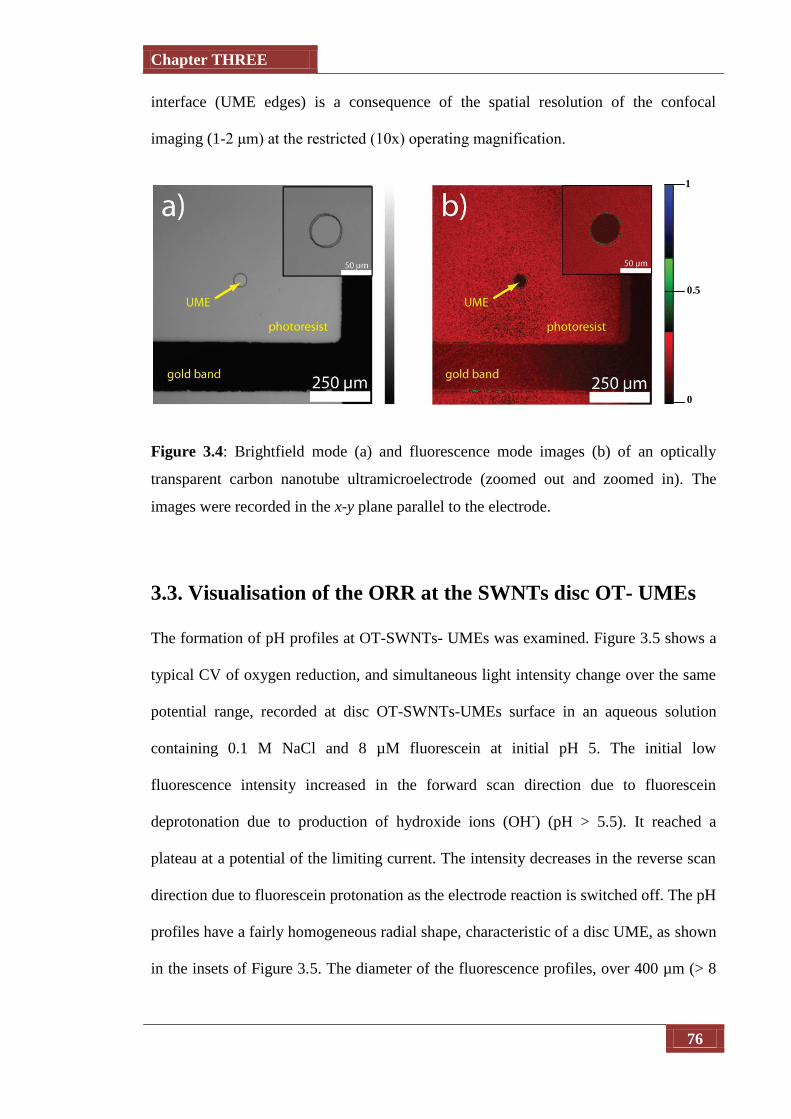
Chapter THREE
76
interface (UME edges) is a consequence of the spatial resolution of the confocal
imaging (1-2 μm) at the restricted (10x) operating magnification.
Figure 3.4: Brightfield mode (a) and fluorescence mode images (b) of an optically
transparent carbon nanotube ultramicroelectrode (zoomed out and zoomed in). The
images were recorded in the x-y plane parallel to the electrode.
3.3. Visualisation of the ORR at the SWNTs disc OT- UMEs
The formation of pH profiles at OT-SWNTs- UMEs was examined. Figure 3.5 shows a
typical CV of oxygen reduction, and simultaneous light intensity change over the same
potential range, recorded at disc OT-SWNTs-UMEs surface in an aqueous solution
containing 0.1 M NaCl and 8 µM fluorescein at initial pH 5. The initial low
fluorescence intensity increased in the forward scan direction due to fluorescein
deprotonation due to production of hydroxide ions (OH-) (pH > 5.5). It reached a
plateau at a potential of the limiting current. The intensity decreases in the reverse scan
direction due to fluorescein protonation as the electrode reaction is switched off. The pH
profiles have a fairly homogeneous radial shape, characteristic of a disc UME, as shown
in the insets of Figure 3.5. The diameter of the fluorescence profiles, over 400 µm (> 8
1
0.5
0
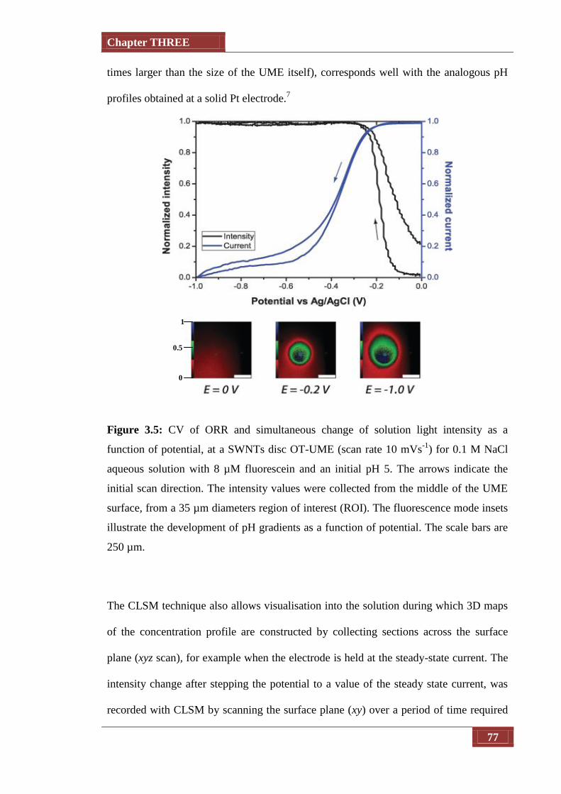
Chapter THREE
77
times larger than the size of the UME itself), corresponds well with the analogous pH
profiles obtained at a solid Pt electrode.7
Figure 3.5: CV of ORR and simultaneous change of solution light intensity as a
function of potential, at a SWNTs disc OT-UME (scan rate 10 mVs-1
) for 0.1 M NaCl
aqueous solution with 8 µM fluorescein and an initial pH 5. The arrows indicate the
initial scan direction. The intensity values were collected from the middle of the UME
surface, from a 35 µm diameters region of interest (ROI). The fluorescence mode insets
illustrate the development of pH gradients as a function of potential. The scale bars are
250 µm.
The CLSM technique also allows visualisation into the solution during which 3D maps
of the concentration profile are constructed by collecting sections across the surface
plane (xyz scan), for example when the electrode is held at the steady-state current. The
intensity change after stepping the potential to a value of the steady state current, was
recorded with CLSM by scanning the surface plane (xy) over a period of time required
1
0.5
0

Chapter THREE
78
for the redox couple to reach a steady-state. Figure 3.6(a) shows a typical 3D map of
fluorescent intensity from fluorescein at, and near to, the OT-SWNTs-UME surface
during the diffusion limited ORR.
Figure 3.6: (a) Fluorescence intensity at a potential of -1.0 V in 0.1 M NaCl solution
with 8 µM fluorescein in the xy, xz and yz planes. The scale bar in the xy image is 250
µm. The red and white lines in xz and yz cross sections indicate the photoresist and OT
UME surface. (b) A graph of intensity below (B) and above (A) the OT-UME plane in
35 µm diameter ROI. The dashed line indicates the electrode surface.
Figure 3.6(b) shows a corresponding cross section of the profile through a 35 µm
diameter ROI, located at the centre of the electrode. CLSM resolution and DNQ
fluorescence impose limitations on the shape of the pH profile in the z direction
(discussed in the following section), however the range of the solution maximum
intensity (pH above 7.5) is ca. 100 µm. Gradual decrease of the intensity further above
the electrode is distinguishable, indicating a decrease of solution pH away from the
electrode area down to a pH value of the bulk solution (pH ca. 5). A dip in the profile
directly above the electrode has been observed as result of excess DNQ fluorescence
around the electrode as can be seen in Figure 3.6 (a).
0.5
1
0
Chapter THREE
79
3.3.1. Dynamic Visualisation of Ru(bpy)32+
concentration during CV
measurements at SWNTs disc OT- UME
Figure 3.7 (a) shows a typical CV (red line) for the oxidation of 10 mM Ru(bpy)32+
in
0.1 M NaCl at a 50 µm diameter disc-shaped OT-SWNTs-UME and a corresponding
solution intensity change (black line) at the electrode surface. The intensity was
measured simultaneously from the centre of the electrode only (35 μm in diameter) to
avoid the contribution of the photoresist luminescent properties coming from the
photoactive component – diazonapthoquinone,76
and the blurring of the UME edges, as
discussed above. The shape of the curve corresponds to a reversible redox system (wave
slope of 59 mV).77
The process is electrochemically reversible; the difference between
the quartile potentials, E3/4 - E1/4, is 59 ± 1 mV and 58 ± 1 mV for forward and reverse
scan directions, respectively.77
The limiting steady-state current, ilim, is ca. 55 nA,
consistent with the value expected at an inlaid disc electrode,77
assuming the diffusion
coefficient, of Ru(bpy)32+
is 5.6 × 10⁻⁶
cm2 s
-1.78
The electrochemical reversibility is
clearly visible also in the intensity signal, which is changing in the opposite direction to
the current change. The initially high intensity of the solution at the electrode surface is
decreasing due to mass transfer of Ru(bpy)32+
species from the bulk to the electrode
surface and oxidation of highly luminescent Ru(bpy)32+
to non-luminescence Ru(III)
oxidation state.
It can clearly be seen that during the forward potential scan, the initial high intensity
(It = 0) of the solution at the electrode surface decreases due to conversion of
Ru(bpy)32+
to Ru(bpy)33+
. The intensity value reaches a minimum plateau at the
potential of the limiting current. In the reverse scan direction Ru(bpy)33+
is converted
back to Ru(bpy)32+
and the intensity increases to the initial, maximum value. The

Chapter THREE
80
reversibility of Ru(bpy)32+
oxidation is evidenced in Figure. 3.8(b) where a linear
relationship between normalised intensity and current values in the range of the quartile
potentials (E1/4 and E3/4) for the forward and reverse scan directions is seen. The nearly
parallel lines in Figure 3.8(b) highlight the reliability of combined CLSM and
electrochemical studies. Similar profiles to the ones shown in the insets of Figure. 3.7(a)
were recorded for lower (1 mM and 5 mM) concentrations of Ru(bpy)32+
. In all cases,
reversible CVs of Ru(bpy)32+
oxidation were obtained, with currents proportional to the
Ru(bpy)32+
concentration.
Figure 3.7: (a) CV (red) and simultaneous change of the fluorescence intensity (black:
scan rate 5 mV/s) for the oxidation of 10 mM Ru(bpy)32+
in aqueous solution in 0.1 M
NaCl. The arrows indicate the forward scan direction. The intensity values were
collected from the 35 µm diameter region of interest at the centre of the UME. Intensity
values and current values were normalised by the initial intensity value at time = 0 s
(It=0) and the steady-state limiting current value (ilim), respectively. The insets show
fluorescence profiles near the OT-SWNTs-UME surface during Ru(bpy)32+
oxidation.
The scale bars are 25 µm. (b) Relationship between normalised current and fluorescence
intensity change for forward andreverse scan directions in the range of quartile
potentials of the voltammetric signature.
b) a)
1
0.5
0

Chapter THREE
81
The insets in Figure 3.7(a) show formation of radial fluorescence profiles that develop
at the OT-SWNTs-UME surface at three potential values. The profiles are formed due
to local depletion of luminescent Ru(bpy)32+
at the electrode. The intensity decrease in
the centre of the OT-CNT-UME at the steady state potential (1.2 V) is due to the
conversion of Ru(bpy)32+
to Ru(bpy)33+
, discussed above.
3.3.2. Three dimensional concentration profiles of Ru(bpy)32+
at the
steady-state current.
The CLSM technique also allows visualisation into the solution. A three dimensional
map of the concentration profile is constructed by collecting sections across the surface
plane (xyz scan) when the electrode is held at the steady-state current. The intensity
change during stepping the potential to a potential of a steady state current, was
recorded with CLSM by scanning the surface plane (xy) over a period of time required
for the redox couple to reach a steady-state. Figure 3.8 illustrates the case for 10 mM
Ru(bpy)3+2
during the initial 5 s quiet time, required for potentiostat stabilisation, the
solution intensity is at its maximum, constant value. After this time, the potential is
stepped to a value of Ru(bpy)32+
oxidation at a diffusion-limited rate (see Figure 3.8). A
simultaneous decrease in the intensity profile to a minimum, value was recorded over
the next few seconds. This period corresponds to the time required for Ru(bpy)32+
oxidation to reach a steady state. The radial concentration profile in the inset in Figure
3.8 depicts a dark domain confined to the electrode area; it illustrates accumulation of
Ru(bpy)3+3
at the electrode surface.
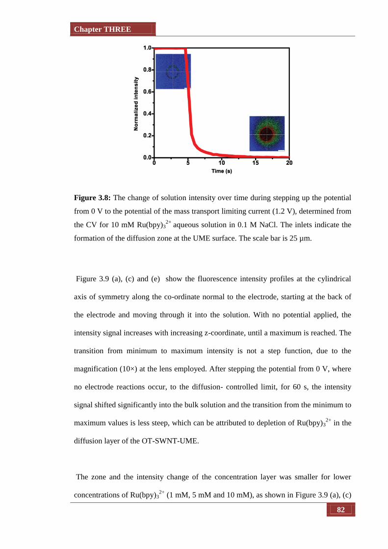
Chapter THREE
82
Figure 3.8: The change of solution intensity over time during stepping up the potential
from 0 V to the potential of the mass transport limiting current (1.2 V), determined from
the CV for 10 mM Ru(bpy)32+
aqueous solution in 0.1 M NaCl. The inlets indicate the
formation of the diffusion zone at the UME surface. The scale bar is 25 µm.
Figure 3.9 (a), (c) and (e) show the fluorescence intensity profiles at the cylindrical
axis of symmetry along the co-ordinate normal to the electrode, starting at the back of
the electrode and moving through it into the solution. With no potential applied, the
intensity signal increases with increasing z-coordinate, until a maximum is reached. The
transition from minimum to maximum intensity is not a step function, due to the
magnification (10×) at the lens employed. After stepping the potential from 0 V, where
no electrode reactions occur, to the diffusion- controlled limit, for 60 s, the intensity
signal shifted significantly into the bulk solution and the transition from the minimum to
maximum values is less steep, which can be attributed to depletion of Ru(bpy)32+
in the
diffusion layer of the OT-SWNT-UME.
The zone and the intensity change of the concentration layer was smaller for lower
concentrations of Ru(bpy)32+
(1 mM, 5 mM and 10 mM), as shown in Figure 3.9 (a), (c)
Chapter THREE
83
and (e), respectively . Figures 3.9 (b), (d) and (f) present a comparison of the intensity
change during the period of the steady state current as a function of the distance from
the electrode, together with the intensity change across the electrode before the potential
step for comparison. In both cases (reaction on or off) no signal is detected far below
the surface, as would obviously be expected. At the steady state current regime the low
intensity of the solution is clearly visible above and just below the UME plane. The
intensity increases less steeply than when no potential is applied (note the position of
the surface in both plots). The maximum intensity value, corresponding to the bulk
solution intensity, is followed by a sudden drop in intensity demonstrating the
absorption of light away from the electrode by Ru(II) species in the bulk solution which
depends on the concentration.
The fluorescence intensity profiles illustrated in Figure 3.9, after and before the
potential step, are indicative of the concentration boundary layer, δ, formed at the OT-
SWNTs-UME, which is of the expected thickness 9.8 µm based on δ=πa/4 (where a is
the electrode radius). Further into the solution, there is a decrease of intensity, in both
profiles, due to light absorption by Ru(bpy)32+
in the bulk solution.2 This convolution of
the response highlights the importance of measuring the concentration (fluorescence)
profiles from the rear of electrode, as demonstrated here.

Chapter THREE
84
Figure 3.9: Cross sectional light intensity change below and above the UME surface
before (left) and after (right) the potential step for the 1 mM (a), 5 mM (c), and 10 mM
(e) Ru(bpy)32+
in 0.1 M NaCl. All images were collected with the z-volume 150 µm
(vertical white dashed line) and the z-step 2 µm. Z-stack before the potential step and
during the steady state for the 1 mM (b), 5 mM (d), and 10 mM (f) Ru(bpy)32+
in 0.1 M
NaCl. The scale bars in (a, c) and (e) are 25 µm. Dark blue arrows indicate the position
b)
d)
f) Off
Off
Off
On
On
On
x z
x z
x
z
x
z
x
z x
z
x
y
x
y
x
y
x
y
x
y
x
y

Chapter THREE
85
of the electrode surface in both scans. The light intensity values were normalised taking
into account the intensity signal from the 35 µm diameter region of interest only.
Notably, studies on Ru(bpy)32+
oxidation (at 10 mM in 0.1 M NaCl) at 25 µm Pt disc
UME revealed strong absorption of the excitation light in the bulk solution, precluding
CLSM visualisation of the redox reaction. Ru(bpy)32+
absorption of the excitation light,
called the primary inner filter effect, was discussed by Amatore et al. in the studies on
dynamics of Ru(bpy)32+
concentration profiles imaged with coherent optical fibres 2.
The authors indicated the local absorbance of the excitation light by Ru(bpy)32+
as the
main factor limiting resolution of fluorescence imaging. Indeed, fluorescence efficiency
of Ru(bpy)32+
is much smaller than for example fluorescein 79
. In both examined cases,
Ru(bpy)32+
oxidation and ORR, a uniform activity of the OT-SWNTs-UMEs mat is
evident. The chronoamperometry (CA) experiments validate the capabilities of CLSM
in studying mass transfer of redox couples. The results thus demonstrate the unique
merit of SWNTs mats as OT-UMEs in monitoring redox reactions which appear
inaccessible with conventional electrochemical set-ups.
3.4. Conclusions
CLSM has proven very useful for quantifying the electrochemical activities of the
SWNTs-UMEs by tracking the dynamic, reversible concentration profiles of
electroactive and photoactive tris(2,2’-bipyridine)ruthenium(II) species during cyclic
voltammetry. Disc-shaped OT-CNT-UMEs have been introduced, through a series of
electrochemical and fluorescence experiments. The SWNTs networks showed both
complete transparency and disc shaped UME characteristics. Visualisation of the mass
transfer processes at the electrode has been achieved using state-of-the-art CLSM. Three
dimensional diffusion profiles of the electroactive and photoactive Ru(bpy)32+
at the

Chapter THREE
86
SWNTs-mat UME were recorded and the optical effects on the imaging resolution were
discussed.
These proof-of-concept experiments broaden the potential applications of the introduced
SWNTs disc UMEs as reliable and effective sensors for broad optical and
electrochemical applications. Further improvement in CLSM resolution and UME
fabrication, for example by using thinner quartz substrates could allow the faithful
measurement of the concentration profiles to be measured with even higher spatial
resolution.

Chapter THREE
87
3.5. References
(1) Amatore, C.; Szunerits, S.; Thouin, L.; Warkocz, J. S. Electroanalysis 2001, 13,
646.
(2) Amatore, C.; Chovin, A.; Garrigue, P.; Servant, L.; Sojic, N.; Szunerits, S.;
Thouint, L. Analytical Chemistry 2004, 76, 7202.
(3) Unwin, P. R.; Macpherson, J. V.; Beeston, M. A.; Evans, N. J.; Littlewood, D.;
Hughes, N. P. Adv Dent Res 1997, 11, 548.
(4) Zhang, J.; Slevin, C. J.; Unwin, P. R. Chemical Communications 1999, 1501.
(5) Fantini, J.; Fournier, D.; Boccara, A. C.; Plichon, V. Electrochimica Acta 1997,
42, 937.
(6) Unwin, P. R.; Macpherson, J. V. Chemical Society Reviews 1995, 24, 109.
(7) Rudd, N. C.; Cannan, S.; Bitziou, E.; Ciani, L.; Whitworth, A. L.; Unwin, P. R.
Analytical Chemistry 2005, 77, 6205.
(8) Grime, J. M. A.; Edwards, M. A.; Rudd, N. C.; Unwin, P. R. Proceedings of the
National Academy of Sciences of the United States of America 2008, 105, 14277.
(9) Engstrom, R. C.; Ghaffari, S.; Qu, H. W. Analytical Chemistry 1992, 64, 2525.
(10) Gabrielli, C.; Ostermann, E.; Perrot, H.; Vivier, V.; Beitone, L.; Mace, C.
Electrochemistry Communications 2005, 7, 962.
(11) Bastos, A. C.; Simoes, A. M.; Gonzalez, S.; Gonzalez-Garcia, Y.; Souto, R. M.
Electrochemistry Communications 2004, 6, 1212.
(12) Rudd, N. C., The University of Warwick, 2007.
(13) Pruiksma, R.; McCreery, R. L. Analytical Chemistry 1979, 51, 2253.
(14) Wu, H. P.; McCreery, R. L. Analytical Chemistry 1989, 61, 2347.
(15) Amatore, C.; Pebay, C.; Servant, L.; Sojic, N.; Szunerits, S.; Thouin, L.
Chemphyschem 2006, 7, 1322.
(16) Texier, F.; Servant, L.; Bruneel, J. L.; Argoul, F. Journal of Electroanalytical
Chemistry 1998, 446, 189.
(17) Amatore, C.; Bonhomme, F.; Bruneel, J. L.; Servant, L.; Thouin, L.
Electrochemistry Communications 2000, 2, 235.
(18) Engstrom, R. C.; Ghaffari, S.; Qu, H. W. Analytical Chemistry 1992, 64, 2525.
(19) Bowyer, W. J.; Xie, J.; Engstrom, R. C. Analytical Chemistry 1996, 68, 2005.
(20) Vitt, J. E.; Engstrom, R. C. Analytical Chemistry 1997, 69, 1070.
(21) Fiedler, S.; Hagedom, R.; Schnelle, T.; Richter, E.; Wagner, B.; Fuhr, G.
Analytical Chemistry 1995, 67, 820.
(22) Cannan, S.; Macklam, I. D.; Unwin, P. R. Electrochemistry Communications
2002, 4, 886.
(23) Amatore, C.; Bonhomme, F.; Bruneel, J. L.; Servant, L.; Thouin, L. Journal of
Electroanalytical Chemistry 2000, 484, 1.
(24) Amatore, C.; Szunerits, S.; Thouin, L.; Warkocz, J. S. Electrochemistry
Communications 2000, 2, 353.
(25) Amatore, C.; Szunerits, S.; Thouin, L. Electrochemistry Communications 2000, 2,
248.
(26) Baltes, N.; Thouin, L.; Amatore, C.; Heinze, J. Angewandte Chemie-International
Edition 2004, 43, 1431.
(27) Engstrom, R. C.; Weber, M.; Wunder, D. J.; Burgess, R.; Winquist, S. Analytical
Chemistry 1986, 58, 844.
(28) Engstrom, R. C.; Meaney, T.; Tople, R.; Wightman, R. M. Analytical Chemistry
1987, 59, 2005.
Chapter THREE
88
(29) Bard, A. J.; Fan, F. R. F.; Kwak, J.; Lev, O. Analytical Chemistry 1989, 61, 132.
(30) Barker, A. L.; Unwin, P. R.; Amemiya, S.; Zhou, J. F.; Bard, A. J. Journal of
Physical Chemistry B 1999, 103, 7260.
(31) Barker, A. L.; Gonsalves, M.; Macpherson, J. V.; Slevin, C. J.; Unwin, P. R.
Analytica Chimica Acta 1999, 385, 223.
(32) Slevin, C. J.; Macpherson, J. V.; Unwin, P. R. Journal of Physical Chemistry B
1997, 101, 10851.
(33) Slevin, C. J.; Unwin, P. R. Langmuir 1997, 13, 4799.
(34) Mayausky, J. S.; McCreery, R. L. J. Electroanal. Chem. 1983, 145, 117.
(35) Jan, C. C.; McCreery, R. L.; Gamble, F. T. Analytical Chemistry 1985, 57, 1763.
(36) Pharr, C. M.; Engstrom, R. C.; Tople, R. A.; Bee, T. K.; Unzelman, P. L. Journal
of Electroanalytical Chemistry 1990, 278, 119.
(37) Engstrom, R. C.; Pharr, C. M.; Koppang, M. D. Journal of Electroanalytical
Chemistry 1987, 221, 251.
(38) Haugland, R. P. Molecular Probes Handbook of Fluorescent Probes and
Research Products,; 9 ed.; Molecular Probes: USA, 2002.
(39) C.M.A. Brett, A. M. O. B. Electrochemistry Principles, Methods and
Applications; OUP: Oxford, 1993.
(40) Gerardi, R. D.; Barnett, N. W.; Lewis, S. W. Analytica Chimica Acta 1999, 378,
1.
(41) Forster, R. J.; Bertoncello, P.; Keyes, T. E. In Annual Review of Analytical
Chemistry 2009; Vol. 2, p 359.
(42) Hiura, H.; Ebbesen, T. W.; Tanigaki, K. Advanced Materials 1995, 7, 275.
(43) Edgeworth, J. P.; Wilson, N. R.; Macpherson, J. V. Small 2007, 3, 860.
(44) Iijima, S. Nature 1991, 354, 56.
(45) Iijima, S.; Ichihashi, T. Nature 1993, 363, 603.
(46) Bethune, D. S.; Kiang, C. H.; Devries, M. S.; Gorman, G.; Savoy, R.; Vazquez, J.;
Beyers, R. Nature 1993, 363, 605.
(47) Bronikowski, M. J.; Willis, P. A.; Colbert, D. T.; Smith, K. A.; Smalley, R. E.
Journal of Vacuum Science & Technology a-Vacuum Surfaces and Films 2001,
19, 1800.
(48) Nikolaev, P.; Bronikowski, M. J.; Bradley, R. K.; Rohmund, F.; Colbert, D. T.;
Smith, K. A.; Smalley, R. E. Chemical Physics Letters 1999, 313, 91.
(49) Scott, C. D.; Povitsky, A.; Dateo, C.; Gokcen, T.; Willis, P. A.; Smalley, R. E.
Journal of Nanoscience and Nanotechnology 2003, 3, 63.
(50) Murakami, Y.; Chiashi, S.; Miyauchi, Y.; Maruyama, S. Japanese Journal of
Applied Physics Part 1-Regular Papers Brief Communications & Review Papers
2004, 43, 1221.
(51) Kong, J.; Soh, H. T.; Cassell, A. M.; Quate, C. F.; Dai, H. J. Nature 1998, 395,
878.
(52) Christoffersen, J.; Christoffersen, M. R.; Arends, J.; Hook, M. Journal of Crystal
Growth 1994, 137, 545.
(53) Snow, E. S.; Novak, J. P.; Campbell, P. M.; Park, D. Applied Physics Letters
2003, 82, 2145.
(54) Shim, Y. B.; Park, S. M. Journal of Electroanalytical Chemistry 1997, 425, 201.
(55) Yoshida, H.; Takeda, S.; Uchiyama, T.; Kohno, H.; Homma, Y. Nano Letters
2008, 8, 2082.
(56) Yoshida, H.; Takeda, S.; Uchiyama, T.; Kohno, H.; Homma, Y. In Nanotubes,
Nanowires, Nanobelts and Nanocoils - Promise, Expectations and Status;
Bandaru, P. R. G. S. K. I., Ed. 2009; Vol. 1142, p 3.
Chapter THREE
89
(57) Dumitrescu, I.; Edgeworth, J. P.; Unwin, P. R.; Macpherson, J. V. Advanced
Materials 2009, 21, 3105.
(58) Dumitrescu, I.; Unwin, P. R.; Macpherson, J. V. Chemical Communications 2009,
6886.
(59) Dumitrescu, I.; Unwin, P. R.; Macpherson, J. V. Electrochemistry
Communications 2009, 11, 2081.
(60) Dumitrescu, I.; Unwin, P. R.; Wilson, N. R.; Macpherson, J. V. Analytical
Chemistry 2008, 80, 3598.
(61) Rutkowska, A.; Bawazeer, T. M.; Macpherson, J. V.; Unwin, P. R. Physical
Chemistry Chemical Physics 2011, 13, 5223.
(62) Rutkowska, A.; Walker, D.; Gorfman, S.; Thomas, P. A.; Macpherson, J. V.
Journal of Physical Chemistry C 2009, 113, 17087.
(63) Day, T. M.; Wilson, N. R.; Macpherson, J. V. Journal of the American Chemical
Society 2004, 126, 16724.
(64) Saito, R.; Fujita, M.; Dresselhaus, G.; Dresselhaus, M. S. Physical Review B 1992,
46, 1804.
(65) Bertoncello, P.; Edgeworth, J. P.; Macpherson, J. V.; Unwin, P. R. Journal of the
American Chemical Society 2007, 129, 10982.
(66) Rosenblatt, S.; Yaish, Y.; Park, J.; Gore, J.; Sazonova, V.; McEuen, P. L. Nano
Letters 2002, 2, 869.
(67) Harlev, E.; Gulakhmedova, T.; Rubinovich, I.; Aizenshtein, G. Advanced
Materials 1996, 8, 994.
(68) Minami, T.; Miyata, T. Thin Solid Films 2008, 517, 1474.
(69) Minami, T. Thin Solid Films 2008, 516, 1314.
(70) Minami, T. Thin Solid Films 2008, 516, 5822.
(71) Shipway, A. N.; Katz, E.; Willner, I. Chemphyschem 2000, 1, 18.
(72) Donner, S.; Li, H. W.; Yeung, E. S.; Porter, M. D. Analytical Chemistry 2006, 78,
2816.
(73) Heras, A.; Colina, A.; Lopez-Palacios, J.; Kaskela, A.; Nasibulin, A. G.; Ruiz, V.;
Kauppinen, E. I. Electrochemistry Communications 2009, 11, 442.
(74) Guell, A. G.; Meadows, K. E.; Unwin, P. R.; Macpherson, J. V. Physical
Chemistry Chemical Physics 2010, 12, 10108.
(75) Vleggaar, J. J. M.; Huizer, A. H.; Varma, C.; Kraakman, P. A.; Nijssen, W. P. N.;
Visser, R. J. Journal of Vacuum Science & Technology B 1993, 11, 688.
(76) Hui, E. E.; Bhatia, S. N. Langmuir 2007, 23, 4103.
(77) Bard, A. J.; Faulkner, L. R. Electrochemical Methods. Fundamentals and
Applications; 2ed ed.; Wiley: India, 2006.
(78) Yan, X.; Li, H.; Xu, Z.; Li, W. Bioelectrochemistry 2009, 74, 310.
(79) Guilbault, G. G. Practical fluorescence; Second ed.; CRC, 1990.

Chapter FOUR
90
Transient Interfacial Kinetics, from Confocal Fluorescence
Visualisation: Application to Proton Attack the Treated Enamel
Substrate 4
Introduction
In this chapter the first use of confocal laser scanning microscopy (CLSM) coupled with
scanning electrochemical microscopy (SECM) is introduced as means of time
dependant visualisation and measurement of proton dispersion on enamel surfaces and
the effectiveness of dissolution inhibitors on enamel substrates. This new technique
provides an analytical method with high spatial and temporal resolution allowing sub-
second analysis of treatment effects on enamel substrates. A decrease of the fluorescein
solution intensity was recorded using CLSM during the oxidation of water at an
ultramicroelectrode (UME). Studies involved measuring pH profiles close to untreated
and treated enamel surfaces. Fluoride and zinc were used as treatments for enamel
surfaces to investigate the effect of inhibitors on proton distribution, since they are
generally considered to impede the dissolution process.
4.1. Overview
Heterogeneous reactions at liquid/solid interfaces are probably one of the main topics in
science and a vast variety of techniques have been applied, mainly focusing on probing
the actual reactive sites.1-2
A reaction at a surface often involves a flux of
molecules/ions from a source (or bulk) towards the reactive sites where the reaction
takes place. The ability to visualize and analyse such processes is crucial for obtaining a
deeper insight into the reaction process. Understanding surface reaction rates is
paramount in a number of fields, such as corrosion,3-5
electrochemical sensors,
electrochemical reactors6 and fuel cells,
6-7 and minerals dissolution.
8-9

Chapter FOUR
91
Of particular interest in both medicinal and electrochemical fields is the mapping of
concentration profiles within the diffusion layer of an active site,10-11
as reviewed
extensively in the preceding chapter. In order to understand dissolution, well-defined
and quantifiable mass transport is the key.12-15
To this extent, the channel flow cell
(CFC) method has proven powerful for studying dissolution processes,12,14
although one
can only measure macroscopic rate over long time period.
Attempts to visualise dynamic proton fluxes have been performed using micro-electrode
ion flux estimators (MIFE) where it is possible to simultaneously measure the flux of
several different ion species,16
but it also requires other ex-situ visualisation techniques
such as SEM and interferometry or profilometry17
and the main drawback of these
methods is the relatively low temporal resolution of c.a. 5 seconds.18
This is particularly
slow in comparison to techniques such as confocal laser scanning microscopy (CLSM)
which has a temporal resolution in the order of milliseconds.19
As highlighted in the
previous chapter, fluorescence CLSM to monitor the concentration profile at an
electrode surface during an electrochemical reaction was successfully introduced by
Unwin and co-workers.20-22
SECM is extensively used as a scanning probe technique for studying dissolution
processes and kinetics 23-27
and visualization of concentration profiles has been probed
down to the micron level. Previous work performed by this group using SECM coupled
with finite element modelling on enamel dissolution, allow the rate of acid attack at
steady-state condition to be quantified.8,28
However, inhibitors can only provide a
temporary barrier layer and it would be very useful to be able to investigate transient
processes and access fast.

Chapter FOUR
92
Enamel proton-induced dissolution has received extensive attention due to its wide
implication in oral science, from caries to acid erosion.8 CLSM has been applied to
many aspects of oral health including dental erosion,29-30
monitoring the differences
between fluoridated and non-fluoridated permanent and deciduous enamel,31
visualizing
enamel rods32
and even to monitor fluid flow through dentine tubules and substances
which subsequently block the tubules.33
Herein, it is shown that by combining CLSM
with UMEs and SECM, greatly enhanced information can be obtained on proton-
induced dissolution and the effect of temporary dissolution barriers from well-known
treatements.
4.1.1. Enamel Structure
The structure of the tooth is shown in Figure 4.1. Enamel is the hardest and most highly
mineralized substance of the body. It is one of the three major tissues which make up
the tooth, along with dentin and dental pulp. It is normally visible and supported by
underlying dentin.
Figure 4.1: A cross sectional schematic of the structure of a tooth; (a) represents the
dental hard tissue enamel, (b) represents the dental soft tissue dentine, (c) is the pulp

Chapter FOUR
93
containing the nerves, (d) is the gum surrounding the tooth and (e) is the bone from
which teeth grow.
Enamel has a prismatic macrostructure arising from its production from ameloblast
cells. Enamel is essentially composed of 95 wt% impure calcium hydroxyapatite (HAP),
Ca10(PO4)6(OH)2 and an the remaining being organic material and water.
4.1.2. Enamel Dissolution
An acidic medium can dissolve hydroxyapatite crystals as per equation 4.1, which is
usually defined as surface demineralization.34
(4.1)
Enamel dissolution can be defined as the localized loss of dental hard tissue35
from the
tooth surface due to the chemical influence of extrinsic acids36
(including acidic
substances, beverages, foods, medication and environmental exposure to acidic agents)
and intrinsic acids36
(including recurrent vomiting as part of the eating disorder bulimia
nervosa or due to the regurgitation of the gastric contents) without the involvement of
microorganisms.36-37
Frequent consumption of acid-containing foods is an important
factor in enamel erosion, with many soft drinks are in the pH range between 2 and 338
being the most commonly consumed erosive acids.37
Dental erosion does not only affect
enamel but can also reach dentine, causing hypersensitivity, or in severe cases, pulp
exposure and even tooth fracture.
Understanding dental erosion would help in the clinical treatment of tooth wear and aid
in the development of new dental restorative materials.33
It would also aid in providing
Chapter FOUR
94
further insights into the chemical process of erosion, and ways in which erosion can be
modified, reduced or prevented. Many techniques have been applied to monitor the
dissolution and precipitation kinetics of enamel and hydroxyapatite and the closely
related fluorapatite, Ca10(PO4)6F2, including techniques of scanning electron
microscopy (SEM)39-41
of enamel surfaces atomic force microscopy (AFM)39-41
profilometry and more recently nanoindentation.39
There have been numerous and
varied studies39,42
quantifying and characterizing the rate, extent and chemical aspects of
enamel erosion.
Typically, the majority of published methods involved subjecting slices of enamel to a
collection of acid challenges,42
ranging in pH from 2.3 to 6.3, or the effect of varying
compositions of solution, and effectively changing the saturation level of the solution.43
Further to this, many studies have included the effect of inhibitory agents and
treatments upon the dissolution of enamel and HAP. However, there is still heated
debate about the quantitative analysis of enamel dissolution, as much of the past work
has involved acid challenges where mass transport is not particularly well-defined. On
the contrary, the work described herein is underpinned by using SECM which is capable
of delivering material to surfaces with well-defined mass transport and thus surface
kinetic effects can readily be distinguished, making quantitative analysis more accurate.
4.1.3. Enamel Dissolution Inhibitors
One of the main objectives of this work is to understand the effect of inhibitors on the
dissolution of enamel. An interesting property of HAP is the ability to exchange
calcium ions by sodium, magnesium, zinc, strontium zinc, or lead ions. Additionally,
hydroxyl and phosphate groups can be substituted by chloride, bicarbonate, and fluoride

Chapter FOUR
95
ions at the apatite surfaces and incorporate in the surface layer in the form of
(zincapatites, fluoroapatites, etc.).44-45
Since the resistance of enamel to acids depends
largely on its chemical composition, it is of interest to determine the composition that
supports or prevents the process of erosion. Fluoride ions are known to be a good
inhibitor of enamel dissolution as it is thought to incorporate into the enamel and
increase the hardness and resistance to acid erosion of the enamel. This incorporation
may involve loosely or firmly bound fluoride, and the extent to which the fluoride
penetrates the enamel is a subject of much debate.31,46-49
4.2. Proton Distribution at Disc UME
The work herein use oxidation of water at the surface of a platinum electrode to
produces protons as indicated in Equation 4.2. This decrease in pH can be monitored as
it causes the disodium fluorescein solution to fluoresce with much less intensity near the
electrode surface, as explained in Chapter 3.
H2O 2H+ + ½ O2 + 2e
(4.2)
Figure 4.2 shows the steady-state fluorescence profile obtained at a 25 μm diameter
platinum disc electrode upon application of anodic currents of 20 nA, 50 nA and 100
nA in an aqueous solution of 8 μM fluorescein with 0.1 M potassium nitrate, at an initial
bulk solution pH of 7.5. A hemispherical fluorescence profile can clearly be seen that
mirrors the diffusion profile at a disc UME.21-22
The fluorescence profile is due to the
generation of protons at the electrode surface and the transition from the light region to
the dark region marks the change in pH from ca pH 7.5 or higher to ca pH 5.5 or lower,
with the midpoint of the boundary at pH 6.1 (see the fluorescence-pH profile, Figure
1.6). The size of the fluorescence profile was found to increase as the applied current
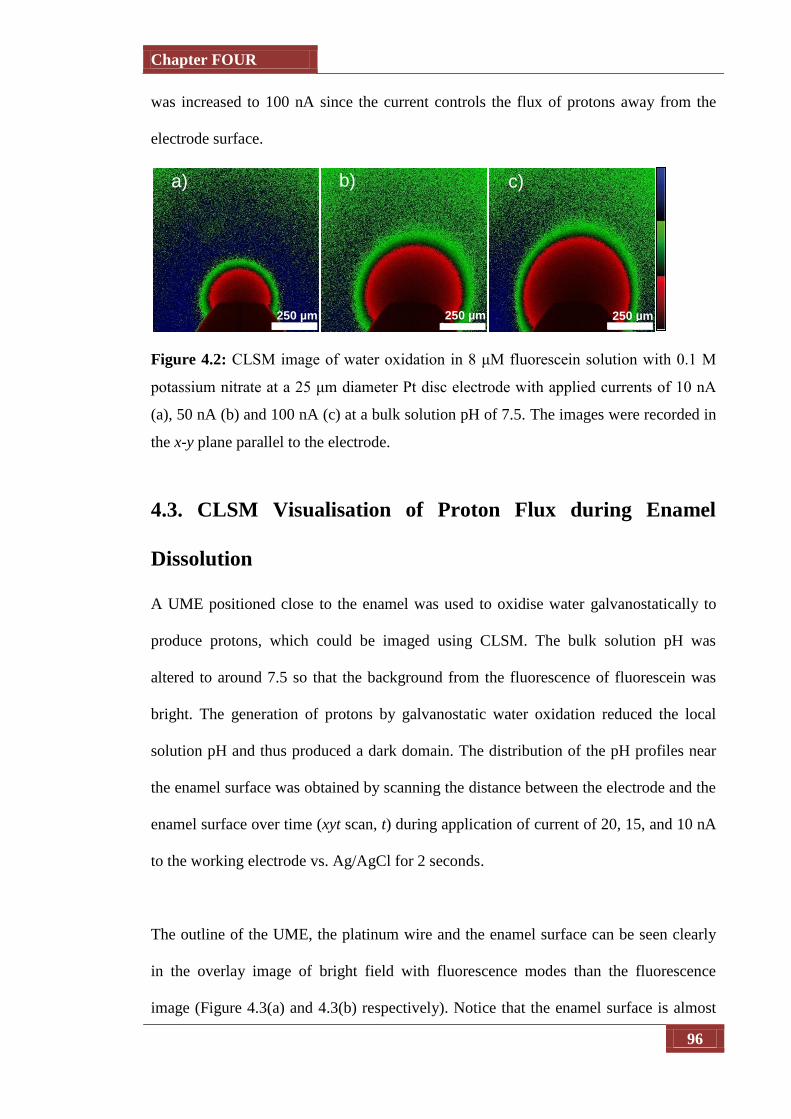
Chapter FOUR
96
was increased to 100 nA since the current controls the flux of protons away from the
electrode surface.
Figure 4.2: CLSM image of water oxidation in 8 μM fluorescein solution with 0.1 M
potassium nitrate at a 25 μm diameter Pt disc electrode with applied currents of 10 nA
(a), 50 nA (b) and 100 nA (c) at a bulk solution pH of 7.5. The images were recorded in
the x-y plane parallel to the electrode.
4.3. CLSM Visualisation of Proton Flux during Enamel
Dissolution
A UME positioned close to the enamel was used to oxidise water galvanostatically to
produce protons, which could be imaged using CLSM. The bulk solution pH was
altered to around 7.5 so that the background from the fluorescence of fluorescein was
bright. The generation of protons by galvanostatic water oxidation reduced the local
solution pH and thus produced a dark domain. The distribution of the pH profiles near
the enamel surface was obtained by scanning the distance between the electrode and the
enamel surface over time (xyt scan, t) during application of current of 20, 15, and 10 nA
to the working electrode vs. Ag/AgCl for 2 seconds.
The outline of the UME, the platinum wire and the enamel surface can be seen clearly
in the overlay image of bright field with fluorescence modes than the fluorescence
image (Figure 4.3(a) and 4.3(b) respectively). Notice that the enamel surface is almost
250 µm
b)
250 µm
a) c)
250 µm
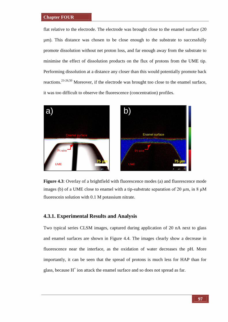
Chapter FOUR
97
flat relative to the electrode. The electrode was brought close to the enamel surface (20
µm). This distance was chosen to be close enough to the substrate to successfully
promote dissolution without net proton loss, and far enough away from the substrate to
minimise the effect of dissolution products on the flux of protons from the UME tip.
Performing dissolution at a distance any closer than this would potentially promote back
reactions.23-26,50
Moreover, if the electrode was brought too close to the enamel surface,
it was too difficult to observe the fluorescence (concentration) profiles.
Figure 4.3: Overlay of a brightfield with fluorescence modes (a) and fluorescence mode
images (b) of a UME close to enamel with a tip-substrate separation of 20 µm, in 8 μM
fluorescein solution with 0.1 M potassium nitrate.
4.3.1. Experimental Results and Analysis
Two typical series CLSM images, captured during application of 20 nA next to glass
and enamel surfaces are shown in Figure 4.4. The images clearly show a decrease in
fluorescence near the interface, as the oxidation of water decreases the pH. More
importantly, it can be seen that the spread of protons is much less for HAP than for
glass, because H+ ion attack the enamel surface and so does not spread as far.
75 µm 75 µm
Enamel surface
UME
Pt wire
a) b)
UME
Pt wire
Enamel surface

Chapter FOUR
98
Figure 4.4 illustrates how protons gradually spread along the glass surface, which forms
a largely impermeable barrier, filling the gap between the UME and the glass substrate
before diffusing into bulk solution. The second series of images, Figure 4.4 (b), in the
case of the enamel shows that the overall spread of protons is more confined as
consequence of the uptake of protons during the dissolution of an enamel sample.
Figure 4.4: Shows a series of images captured from the CLSM at times of 0 sec, when
no current has passed, 1.22 seconds, 1.64 seconds, 2.89 seconds and 4.57 seconds (a)
The proton distribution next to glass substrate, (b) The proton dispersion near to an
enamel substrate. The yellow scale bar represents 75 m.
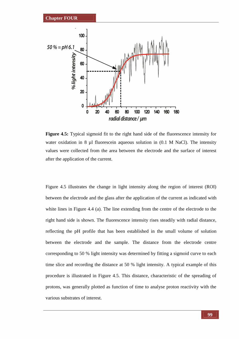
Chapter FOUR
99
Figure 4.5: Typical sigmoid fit to the right hand side of the fluorescence intensity for
water oxidation in 8 µl fluorescein aqueous solution in (0.1 M NaCl). The intensity
values were collected from the area between the electrode and the surface of interest
after the application of the current.
Figure 4.5 illustrates the change in light intensity along the region of interest (ROI)
between the electrode and the glass after the application of the current as indicated with
white lines in Figure 4.4 (a). The line extending from the centre of the electrode to the
right hand side is shown. The fluorescence intensity rises steadily with radial distance,
reflecting the pH profile that has been established in the small volume of solution
between the electrode and the sample. The distance from the electrode centre
corresponding to 50 % light intensity was determined by fitting a sigmoid curve to each
time slice and recording the distance at 50 % light intensity. A typical example of this
procedure is illustrated in Figure 4.5. This distance, characteristic of the spreading of
protons, was generally plotted as function of time to analyse proton reactivity with the
various substrates of interest.
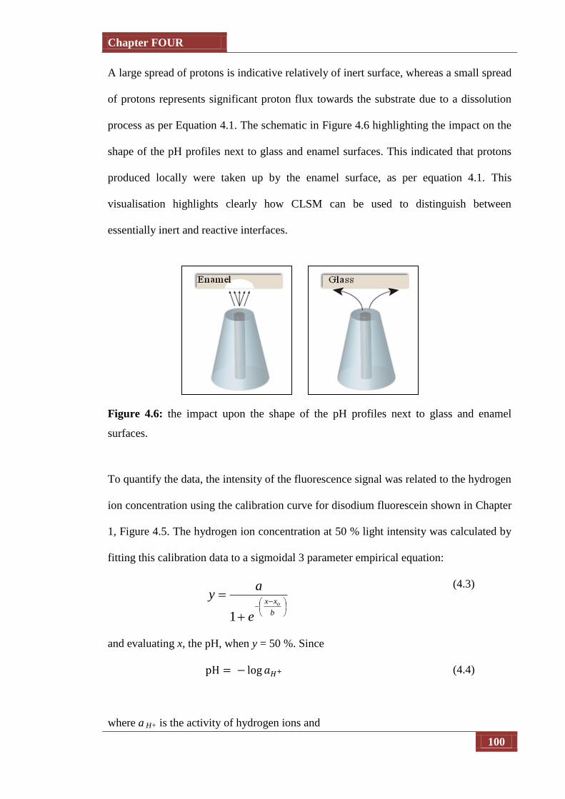
Chapter FOUR
100
A large spread of protons is indicative relatively of inert surface, whereas a small spread
of protons represents significant proton flux towards the substrate due to a dissolution
process as per Equation 4.1. The schematic in Figure 4.6 highlighting the impact on the
shape of the pH profiles next to glass and enamel surfaces. This indicated that protons
produced locally were taken up by the enamel surface, as per equation 4.1. This
visualisation highlights clearly how CLSM can be used to distinguish between
essentially inert and reactive interfaces.
Figure 4.6: the impact upon the shape of the pH profiles next to glass and enamel
surfaces.
To quantify the data, the intensity of the fluorescence signal was related to the hydrogen
ion concentration using the calibration curve for disodium fluorescein shown in Chapter
1, Figure 4.5. The hydrogen ion concentration at 50 % light intensity was calculated by
fitting this calibration data to a sigmoidal 3 parameter empirical equation:
b
xx o
e
ay
1
(4.3)
and evaluating x, the pH, when y = 50 %. Since
(4.4)
where a H+ is the activity of hydrogen ions and

Chapter FOUR
101
(4.5)
Taking the activity coefficient of hydrogen ions (H+) as 0.75 51
in 0.1 mol dm3
aqueous solutions, the hydrogen ion concentration corresponding to 50 % fluorescent
light intensity is 7.9 x 10⁷
mol dm3
for disodium fluorescein solution, equivalent to pH
6.1. The plots of the radial distances at 50 % light intensity, as a function of time from
the applied current, produced a spatio-temporal profile for a hydrogen ion concentration
of 7.9 x 10⁷
mol dm3
.
Shown in Figure 4.7 (a) are the variation of proton diffusion front (and hence pH) as a
function of time for a 20 nA current showing the inherent differences between an
untreated surface, a surface treated with 1000 ppm (0.053 M equivalent) NaF or 0.01 M
ZnCl2 (1363 ppm equivalent). In particular, it can be seen that the proton diffusion
expands more in case of the treated samples (at least initially) than untreated. This
indicates that fluoride and zinc treated enamel provides more resistance to acid attack
(less uptake of protons) than untreated enamel alone (more uptake of protons).
0.0 0.5 1.0 1.5 2.0 2.5
0
20
40
60
80
100
120
Ra
dia
l d
istn
ce
m
time/s
20 nA Treated Enamel with Zn
20 nA Treated Enamel with F
20 nA Untreated Enamel
(a)
][ Ha
HH

Chapter FOUR
102
Figure 4.7: Radial distance-time profile of the distance dependence of the pH 6.1 front
in a thin layer of aqueous solution following the oxidation of water at a 25 μm diameter
Pt UME, positioned 20 μm away from untreated enamel (black squares, black line),
fluoride-treated enamel (red circles, red line) and zinc-treated enamel (blue triangles,
blue line). Current applied: Current applied: (a) 20 nA , (b) 15 nA and (c) 10 nA.
The proton profile with fluoride is interesting because spreads initially to 85 which last
for only ca. 1 s then the profile is less extensive. This indicates the fluoride barrier is
only temporary and is eroded quickly with proton uptake becoming comparable to that
0.0 0.5 1.0 1.5 2.0 2.5
0
20
40
60
80
100
120
Ra
dia
l d
ista
ncem
time/s
15 Treated with Zn
15 nA Untreared
15 nA Treated with F
0.0 0.5 1.0 1.5 2.0 2.5
0
20
40
60
80
100
Ra
dia
l d
ista
ncem
time/s
15 Treated with Zn
15 nA Untreared
15 nA Treated with F
0.0 0.5 1.0 1.5 2.0 2.5
0
20
40
60
80
100
120
Ra
dia
l d
ista
nc
e m
m
time/s
10 nA Treated Enamel with Zn
10 nA Untreated Enamel
10 nA Treated Enamel with F
(b)
(c)

Chapter FOUR
103
of untreated enamel. Thus fluoride provides only a temporary protection toward acid
attack. Further evidence for this action of fluoride as protective is evident in Figure 4.7
(b) and (c) where lower proton fluxes are used. It can be seen that for decreasing current
(proton flux) the fluoride barrier lasts longer. Interestingly, one of the significant
outcomes of the studies reported here is that F- is able to provide only a very temporary
barrier, whereas in case of zinc the spread of proton traveled a larges radial distance and
lasts longer time, indicating the surface is considerably less active and less susceptible
to interaction with protons.
4.4. Finite Element Model
The geometry for the finite element model developed, which included a moving
boundary (etch pit, but this was not used) is shown in Figure 4.8. The model was run
under specific conditions corresponding to those used experimentally. The simulation
domain is shown in Figure 4.8. The boundary conditions are listed in Table 4.1 and the
numbers represent the boundaries referred to in Figure 4.8 when defining boundary
conditions. Edge 2 represents the shape of the substrate geometry at the initial time and
after simulation of acid etching for some time. The labels used to characterize the
geometry are: a, the radius of the metallic portion of the disk electrode; RG is the ratio
of the radius of the entire probe to that of the wire; and h is the distance between tip and
substrate prior to etching.
Numerical simulations were performed on a Dell Intel Core 2 Duo 2.53 GHz computer
equipped with 8 GB of RAM and running Windows XP Professional 64 Bit 2002
edition. Modeling was performed using the commercial finite element package Comsol
Multiphysics 3.5a (Comsol AB, Sweden), using the Matlab interface (Release 2009a)
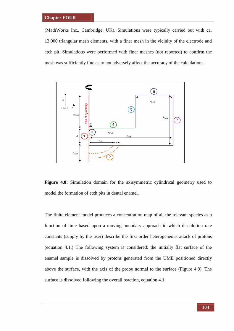
Chapter FOUR
104
(MathWorks Inc., Cambridge, UK). Simulations were typically carried out with ca.
13,000 triangular mesh elements, with a finer mesh in the vicinity of the electrode and
etch pit. Simulations were performed with finer meshes (not reported) to confirm the
mesh was sufficiently fine as to not adversely affect the accuracy of the calculations.
Figure 4.8: Simulation domain for the axisymmetric cylindrical geometry used to
model the formation of etch pits in dental enamel.
The finite element model produces a concentration map of all the relevant species as a
function of time based upon a moving boundary approach in which dissolution rate
constants (supply by the user) describe the first-order heterogeneous attack of protons
(equation 4.1.) The following system is considered: the initially flat surface of the
enamel sample is dissolved by protons generated from the UME positioned directly
above the surface, with the axis of the probe normal to the surface (Figure 4.8). The
surface is dissolved following the overall reaction, equation 4.1.
hUME
hsurf
d
rUME
rpit
rbulk
hbulk
rsurf
a
Chapter FOUR
105
The model assumes that there is a uniform flux, j, of protons at the electrode surface,
(4.6)
where I is the applied current, n the number of electrons transferred, F is Faraday’s
constant and A the area of the electrode. This has been shown to be reasonable in many
previous studies. 21
The equation solved on the interior of the domain illustrated in Figure 4.8 is the time-
dependent reaction diffusion equation cast in axisymmetric coordinates (equation 4.7):
(4.7)
where i is the species under consideration (H+, HnPO4
3-n), and Ci represents the
concentration of species i, Ca2+
, H+, OH
-, HPO4
2-, H2PO4
-, H3PO4, Ca
2+, or the ion pairs
and [Ca2+
H2PO4-]. Di represents the diffusion coefficient of species i, and Ri is the net
production of species i via equilibrium reactions (ie amount of i produced – amount of i
used up).
In Table 4.1, the geometric quantities hsurf, d, hUME, rUME, a, rpit, and rsurf represent the
height of the surface, the UME-surface separation, the height of the UME, the radius of
the active UME microwire, the radius of the etch pit and the radius of the surface
respectively. Boundaries 6 and 7 were set at a sufficient distance from the region of
interest so as to obtain a good solution.
nFA
Ij
iiii RCD
t
C
2

Chapter FOUR
106
Table 4.1: Boundary conditions for finite element modeling.
Boundary
Description
Number in
Figure 4.8
Coordinates Equation
Axis of
symmetry
(fixed in r but
free in z)
1 r=0
(hsurf+d+hUME)>z>0
Solution/enamel
interface
(moving)
2 r = rpit
z = hsurf
For H+:
For H2PO4-:
For HPO42-
and H3PO4:
Solution/active
electrode
interface
(fixed)
3 r=a
z = hsurf + d
For H+:
For HnPO43-n
:
Solution/insulato
r interface
(fixed)
4 & 5 r = rUME
For 4: z = hsurf + d
For 5:
z = hsurf + d + hUME
Bulk solution
(fixed)
6 r = rsurf
z = hsurf + d + hUME
For H+:
For HnPO43-n
:
Bulk solution
(fixed in r but
free in z)
7 r = rsurf
z = hsurf + d + hUME
For H+:
For HnPO43-n
:
nC 0
nCDkCHHH
nCDCkPOHPOHH
42428
6
nC 0
areaF
i
z
CD H
H
nCi 0
nCi 0
pHbulkHC 10
0iC
pHbulkHC 10
0iC

Chapter FOUR
107
4.4.1 Diffusion Coefficients
The following set of equations describes all possible equilibria for the numerical
model:52
HPO42-
PO43-
+ H+
pKa = 12.32
(4.8)
H2PO4- HPO4
2- + H
+ pKa = 7.21
(4.9)
H3PO4 H2PO4- + H
+ pKa = 2.16
(4.10)
[Ca2+
OH-] Ca
2+ + OH
- pKeq = 1.29
(4.11)
H2O OH- + H
+ pKw = 14
(4.12)
[Ca2+
PO43-
] Ca2+
+ PO43-
pKeq = 6.42
(4.13)
[Ca2+
HPO42-
] Ca2+
+ HPO42-
pKeq = 2.64
(4.14)
[Ca2+
HPO4-] Ca
2+ + H2PO4
- pKeq = 1.34 (4.15)
The pKa of equation 4.8 is so high that at the pH range we are working within (pH < 7)
there is no need to consider this reaction, thus the fully deprotonated PO43-
species was
not modelled. Similarly, the pH range of interest and pKeq value of equation 4.11
dictates that the equilibrium will be all the way to the right and thus the ion pair [Ca2+
OH-] is not considered. Equation 4.13 was also disregarded as PO4
3- need not be
considered (vide supra). The pKa values of all species were corrected for ionic activity
with the Davies equation 53-54
given the presence of 0.1 M NaNO3. The influence of the
protonation / deprotonation state of fluorescein was found to have no significant effect
on the results due to the very low concentration of that species (µm) and was therefore
ignored in the calculations. The diffusion coefficients used in the model are given in
Table 4.2.55

Chapter FOUR
108
Table 4.2: Diffusion coefficients of all species considered in the model in units of cm2
s-1
.
Species Diffusion Coefficeint / cm2 s
-1
HD 7.60 x 10
-5
OHD 5.00 x 10
-5
2CaD 7.92 x 10
-6
2+ 24{Ca HPO }
D 1.00 x 10⁻⁵
2+2 4
}{Ca H POD 1.00 x 10
-5
3 4H POD 8.24 x 10⁻⁶
2 4H POD 8.24 x 10
-6
24HPO
D 8.24 x 10⁻⁶
We set the diffusion coefficients of any ion pairs to 1.0 x 10⁻⁵
cm2 s
-1, which is a typical
value for entities of this size,55-56
because such species play a minor role the simulations
were relatively insensitive to the magnitude of these diffusion coefficients. The most
important diffusion coefficient is that for H+ which drives the dissolution process and
for which we have highly accurate values.

Chapter FOUR
109
4.4.2. Insights from Simulations
The finite element model produces pH profiles as a function of time for rate constants of
dissolution for untreated and treated enamel. The fluorescence intensity (I) map was
calculated from the model output (pH profile) via the calibration curve discussed above.
Time resolved dissolution kinetics rates were extracted by matching the experimental
intensity data to the numerical solutions. The model produces pH profiles as a function
of time for rate constants of dissolution for untreated and treated enamel. These
theoretical data were also used to plot radial distance from the electrode centre, against
time, for a specific proton concentration.
Figures 4.9 shows the displacements of 50% intensity profiles measured experimentally
at untreated, fluoride treated and zinc treated enamel respectively for a current of 20 nA,
fitted by the modelled displacement for the 50 % light intensity described earlier with
rate constant (in the range 0.001-1 cm s-1
). It can be seen that the 50% intensity expands
with time, as expected for a proton induced dissolution process, such that these profiles
travel less radial distance with increasing Kvert. This is because a larger rate constant
leads to greater consumption of protons at the substrate surface. Therefore, as can be
seen in cases of treated samples, the presence of the inhibitors significantly retards the
rate of enamel dissolution. This has slowed considerably from 0.2 cm s-1
for untreated
enamel, down to 0.03 cm s-1
for Zn treated enamel and between 0.02 cm s-1
cm s-1
and
0.05 cm s-1
for 1000 ppm NaF treated enamel at short time.
Figure 4.9 (a) shows indicative results from the matching of experimental and simulated
fluorescence profiles next to untreated enamel with a rate constant of dissolution
between 0.08 and 1 cm s-1
, averaging at 0.2 cm s-1
with an averaged proton spread of 66

Chapter FOUR
110
µm for untreated enamel. It can be seen that the experimental 50% intensity profiles and
the simulation are generally in good agreement. A minor discrepancy is that the profile
of the experimental is slightly lower than predicted by theory at short time, before 0.2 s.
The consistency of this behaviour across a number of profiles and for a range of
currents gives confidence that the factor that could influence this is the possible surface
processes which are not related to dissolution. This can be related due to polishing the
surface before performing the experiment, as this is consistent with all experiment
performed herein.
Figure 4.9 (b) shows the initial layer of fluoride protecting the surface by allowing the
protons to spread out to 84 µm, equivalent to the closest match for the vertical rate
constant kvert between 0.02 cm s-1
and 0.05 cm s-1
. Treating the surface with fluoride
increases the proton spread on the surface and considerably slows the rate of
dissolution, however this protection only lasts up to c.a. 1 second after which the proton
spread averages 67 µm and a rate constant match comparable to untreated enamel of 0.2
cm s-1
. Figure 4.9 (c) details the rate constant of dissolution for zinc treated enamel to
be 0.03 cm s-1
, interestingly this rate is in the range of the initial protection from
fluoride treatment however the overall proton spread for zinc treatment averages at 103
µm. That is the largest proton spread we have encountered and is suggestive of a surface
that is considerably less active.

Chapter FOUR
111
Figure 4.9: Radial distance-time profile of the distance dependence of the pH 6.1 front
in a thin layer of aqueous solution following the oxidation of water at a 25 μm diameter
Pt UME, matched to their respective rate constants were the experimental data is shown
0.0 0.5 1.0 1.5 2.0
0
40
80
120Experimental Data
kvert
= 0.05 cm s-1
kvert
= 0.08 cm s-1
kvert
= 0.2 cm s-1
kvert
= 1 cm s-1
Ra
dia
l d
ista
nce
/ µ
m
time / sec
0.0 0.5 1.0 1.5 2.0
0
40
80
120
160
Experimental Data
kvert
= 0.01 cm s-1
kvert
= 0.02 cm s-1
kvert
= 0.05 cm s-1
kvert
= 0.2 cm s-1
kvert
= 1 cm s-1
Radia
l d
ista
nceµ
m
time / sec
(a)
(b)
(c)
0.0 0.5 1.0 1.5 2.0
0
40
80
120
160
Ra
dia
l d
ista
nce
/ µ
m
time / sec
Experimental Dtat
kvert
= 0.01 cm s-1
kvert
= 0.03 cm s-1
kvert
= 0.05 cm s-1
kvert
= 0.2 cm s-1

Chapter FOUR
112
as black squares and (a) is untreated enamel (b) is the fluoride treated enamel (c) is the
zinc treated enamel. Current applied: 20 nA.
As mentioned previously, all experiments were carried out at three currents, 20 nA, 15
nA and 10 nA. For all currents applied, the rate of lateral diffusion was faster at an
untreated, than at fluoride treated and zinc treated enamel. The details of the averaged
rate constant and distance that the protons spread at 50 % intensity (pH 6.1) is given in
Table 4.3 for the three different surfaces at the three different rate constants. The rate
constant data for fluoride is expressed as the slowest rate at the peak to the average rate
after 1 second, this is also true of the distance of proton spread data. It is clear from the
table that the lower the current is, the higher the pH which leads to longer protection
time of fluoride.
Table 4.3: Proton distribution (50 % intensity; pH 6.1) and rate constant match for each
of the three currents, 10, 15 and 20 nA over the three different surfaces and after 4 s.
Current used nA Surface Treatment Proton Spread / µm Rate Constant / cm s-1
10 Untreated 57 0.3
10 Fluoride 75 - 60 0.02 - 0.08
10 Zinc 87 0.03
15 Untreated 61 0.3
15 Fluoride 83 - 65 0.03 - 1
15 Zinc 96 0.03
20 Untreated 66 0.2
20 Fluoride 84 - 67 0.02 - 0.2
20 Zinc 103 0.03
Chapter FOUR
113
4.5. Amount of Zinc and Fluoride Uptake on Treated Enamel
It was shown above that fluoride provided only a very temporary barrier, whereas Zn2+
treatment results in a more permanent barrier. It is thus important to elucidate why there
is this difference and elucidate how much Zn2+
and F- is taken up by enamel due to
these treatments. When treating the enamel sample with 5 ml of 10 mM ZnCl2, 0.183
ppm (2.798 × 10⁻⁶
mol L-1
) of Zn2+
was found absorbed (measured using inductively
coupled plasma mass spectrometry, ICP-MS). Thus, the total amount of Zn2+
absorbed
by the enamel sample in the area exposed to the solution of 4.57 × 10⁻⁴
m2 was
calculated to be 1.4 × 10⁻⁸
mol. In order to equate the amount of zinc take up to an
overall depth of penetration, the molar volume MV was calculated:
(4.14)
where MM is the molar mass of enamel (1004 g mol-1
) 57
and ρ is the density of enamel
(28000 g m-3
). This gave the molar volume as 3.58 × 10⁻⁴
m-3
mol-1
. Taking account of 10
Ca2+
in each HA can be exchanged with zinc, as per equation 1.1. The molar volume is
multiplied by the total amount absorbed on enamel sample 1.4 × 10⁻⁸
mol and divided
by the surface area 0.00457 m2 to give an overall depth of penetration of 1.1×10
-5 m for
pre-treatment with 10 mM.
Interestingly when treating an enamel sample with 26 mM NaF, only 92 ppm
(4.843×10⁻³
mol L-1
) is actually absorbed (measured using a fluoride ion selective
electrode (FISE)). The overall depth of penetration of 1.8 × 10⁻³
m was calculated for
pre-treatment with 26 mM for enamel disc sample of diameter of ca. 6.76 ×10⁻³
m as
detailed in previous work.56
Even though the overall depth of penetration of zinc is less
than fluoride, this suggests that the zinc substitution forms a more stable molecule
which is better at resisting acid attack, in comparison to untreated or fluoride treated

Chapter FOUR
114
enamel. Zinc is known to be readily taken up by HA and competes with calcium ion
(facilitated by the similarities in ionic size between zinc and calcium) for surface
positions on the crystals surface. Zinc can substitute in for calcium in the apatite lattice
and form zinc hydroxyapatite matrix and this formation of zinc apatite is proving to be
more resistant to acid attack than the fluoride substituted hydroxides in the enamel
matrix, commonly known as fluroapatite.57
4.6. Conclusions
SECM has been successfully combined with CLSM to image proton diffusion in a thin
layer of solution at the surface of enamel. This new technique provides an analytical
method with high spatial and temporal resolution permitting sub-second analysis of
treatment effects on enamel substrates. It permits direct visualisation of the surface
reaction and presents itself as a new technique for assessing the proton dispersion on
surfaces and indeed for assessing the effectiveness of inhibitors on substrates. The
method developed uses microelectrode generated pH challenges combined with CLSM
to image proton diffusion and dissolution at the surface of enamel. Specially, localised
dissolution of dental enamel has been achieved by the application of a proton flux to the
enamel surface from a UME positioned in close proximity to the enamel surface. It has
been shown that fluoride and zinc change the morphology of the fluorescent profile that
forms compared to untreated enamel, due to their barrier effect, in which they protect
enamel to same extent.
Modelling of the data using the theoretical finite element model Comsol has indicated
that acid erosion does occur at both untreated and treated enamel surfaces, but in the
treated cases this is slower than the rate of dissolution at untreated enamel. Rate

Chapter FOUR
115
constants of dissolution were assigned for each of the three different surface treatments
at the three different currents of 10, 15 and 20 nA. Zinc treated enamel proved itself to
provide a more resistant barrier to proton attack than the fluoride treatment, even though
the surface concentration and depth of penetration of fluoride in enamel was much more
extensive than that of Zn2+
. Fluoride showed itself to be an initial barrier to proton with
rate constant similar to zinc, however this barrier only lasted for approximately one
second for the range of quite high proton fluxes applied, before returning to a rate
comparable to that of untreated enamel. This suggests that zinc substitution into the HA
matrix creates a strong material, presumably zinc apatite, which is more resistive to
proton attack than fluoride treated enamel. These experiments broaden the potential
applications of CLSM in assessing the proton dispersion on surfaces and indeed for
assessing the effectiveness of inhibitors on substrates.

Chapter FOUR
116
4.7. References
(1) Hulsken, B.; Van Hameren, R.; Gerritsen, J. W.; Khoury, T.; Thordarson, P.;
Crossley, M. J.; Rowan, A. E.; Nolte, R. J. M.; Elemans, J. A. A. W.; Speller, S.
Nature Nanotechnology 2007, 2, 285.
(2) Elemans, J. A. A. W. Materials Today 2009, 12, 34.
(3) Pidaparti, R.; Neblett, E.; Miller, S.; Alvarez, J. Smart. Mater. Struct. 2008, 17.
(4) Lillard, R. S.; Willcutt, G. J.; Pile, D. L.; Butt, D. P. Journal of Nuclear Materials
2000, 277, 250.
(5) Lillard, S.; Gac, F.; Paciotti, M.; Ferguson, P.; Willcutt, G.; Chandler, G.;
Daemen, L. In Effects of Radiation on Materials: 20th International Symposium;
Rosinski, S. T. G. M. L. A. T. R. K. A. S., Ed. 2001; Vol. 1045, p 631.
(6) Kreuer, K. D. Chemistry of Materials 1996, 8, 610.
(7) Wu, H. P.; McCreery, R. L. Analytical Chemistry 1989, 61, 2347.
(8) McGeouch, C.-A.; Edwards, M. A.; Mbogoro, M. M.; Parkinson, C.; Unwin, P. R.
Analytical Chemistry 2010, 82, 9322.
(9) Bengtsson, A.; Sjoberg, S. Pure and Applied Chemistry 2009, 81, 1569.
(10) Abou-Hassan, A.; Dufreche, J. F.; Sandre, O.; Meriguet, G.; Bernard, O.; Cabuil,
V. Journal of Physical Chemistry C 2009, 113, 18097.
(11) Amatore, C.; Pebay, C.; Servant, L.; Sojic, N.; Szunerits, S.; Thouin, L.
Chemphyschem 2006, 7, 1322.
(12) Compton, R. G.; Unwin, P. R. Journal of Electroanalytical Chemistry 1986, 205,
1.
(13) Snowden, M. E.; Unwin, P. R.; Macpherson, J. V. Electrochemistry
Communications 2011, 13, 186.
(14) Mbogoro, M. M.; Snowden, M. E.; Edwards, M. A.; Peruffo, M.; Unwin, P. R.
Journal of Physical Chemistry C 2011, 115, 10147.
(15) Snowden, M. E.; King, P. H.; Covington, J. A.; Macpherson, J. V.; Unwin, P. R.
Analytical Chemistry 2010, 82, 3124.
(16) Newman, I. A. Plant. Cell. Environ. 2001, 24, 1.
(17) Shellis, R. P.; Finke, M.; Eisenburger, M.; Parker, D. M.; Addy, M. European
Journal of Oral Sciences 2005, 113, 232.
(18) Shabala, L.; Roos, T.; McMeekin, T. Microbiol. Aus. 2004.
(19) Pawley, J. Handbook of Biological Confocal Microscopy; 3rd ed.; Springer:
Winconsin, 2006.
(20) Grime, J. M. A.; Edwards, M. A.; Rudd, N. C.; Unwin, P. R. Proceedings of the
National Academy of Sciences of the United States of America 2008, 105, 14277.
(21) Rudd, N. C.; Cannan, S.; Bitziou, E.; Ciani, L.; Whitworth, A. L.; Unwin, P. R.
Analytical Chemistry 2005, 77, 6205.
(22) Cannan, S.; Macklam, I. D.; Unwin, P. R. Electrochemistry Communications
2002, 4, 886.
(23) Macpherson, J. V.; Unwin, P. R. Journal of Physical Chemistry 1994, 98, 11764.
(24) Macpherson, J. V.; Unwin, P. R. Journal of Physical Chemistry 1994, 98, 1704.
(25) Macpherson, J. V.; Unwin, P. R. Journal of Physical Chemistry 1995, 99, 14824.
(26) Macpherson, J. V.; Unwin, P. R. Progress in Reaction Kinetics and Mechanism
1995, 20, 185.
(27) Macpherson, J. V.; Unwin, P. R. Journal of Physical Chemistry 1996, 100, 19475.
(28) McKelvey, K.; Edwards, M. A.; Unwin, P. R. Analytical Chemistry 2010, 82,
6334.

Chapter FOUR
117
(29) Hjortsjo, C.; Jonski, G.; Thrane, P. S.; Saxegaard, E.; Young, A. Caries Research
2009, 43, 449.
(30) Heurich, E.; Beyer, M.; Jandt, K. D.; Reichert, J.; Herold, V.; Schnabelrauch, M.;
Sigusch, B. W. Dental Materials 2010, 26, 326.
(31) Sonju Clasen, A. B.; Ogaard, B.; Duschner, H.; Ruben, J.; Arends, J.; Sonju, T.
Advances in dental research 1997, 11, 442.
(32) Radlanski, R. J.; Renz, H.; Willersinn, U.; Cordis, C. A.; Duschner, H. European
Journal of Oral Sciences 2001, 109, 409.
(33) Williams, C. G.; Macpherson, J. V.; Unwin, P. R.; Parkinson, C. Analytical
Sciences 2008, 24, 437.
(34) Margolis, H. C.; Zhang, Y. P.; Lee, C. Y.; Kent, R. L.; Moreno, E. C. Journal of
Dental Research 1999, 78, 1326.
(35) Mahoney, E. K.; Kilpatrick, N. M. New Zealand Dental Journal 2003, 99, 33.
(36) Davis, R. E.; Marshall, T. A.; Qian, F.; Warren, J. J.; Wefel, J. S. Journal of the
American Dental Association 2007, 138, 1593.
(37) Wongkhantee, S.; Patanapiradej, V.; Maneenut, C.; Tantbirojn, D. Journal of
Dentistry 2006, 34, 214.
(38) Rubinstein, E.; Hauge, C.; Sommer, P.; Mortensen, T. Pharmacology &
Toxicology 1993, 72, 61.
(39) Cheng, Z. J.; Wang, X. M.; Cui, F. Z.; Ge, J.; Yan, J. X. Biomedical Materials
2009, 4.
(40) Attin, T.; Becker, K.; Hannig, C.; Buchalla, W.; Hilgers, R. Caries Research
2005, 39, 432.
(41) Wang, L. J.; Tang, R. K.; Bonstein, T.; Orme, C. A.; Bush, P. J.; Nancollas, G. H.
Journal of Physical Chemistry B 2005, 109, 999.
(42) Barbour, M. E.; Parker, D. M.; Allen, G. C.; Jandt, K. D. European Journal of
Oral Sciences 2003, 111, 428.
(43) Barbour, M. E.; Parker, D. M.; Jandt, K. D. Journal of Colloid and Interface
Science 2003, 265, 9.
(44) Amjad, Z.; Koutsoukos, P. G.; Nancollas, G. H. Journal of Dental Research 1981,
60, 450.
(45) LeGeros, R. Z. Journal of Dental Research 1990, 69 Spec No, 567.
(46) Hannig, C.; Hamkens, A.; Becker, K.; Attin, R.; Attin, T. Archives of Oral
Biology 2005, 50, 541.
(47) Duschner, H.; Gotz, H.; Ogaard, B. European Journal of Oral Sciences 1997, 105,
466.
(48) Tanaka, M.; Moreno, E. C.; Margolis, H. C. Archives of Oral Biology 1993, 38,
863.
(49) Ten Cate, J. M. Acta Odontologica Scandinavica 1999, 57, 325.
(50) Unwin, P. R.; Macpherson, J. V.; Martin, R. D.; McConville, C. F. Electrochem.
Soc. 2000, 99, 104.
(51) Harnad, H. S. O., W. The Physical Chemistry of Electrolytic Solutions; Reinhold
Publishing Corp: New York, 1950.
(52) Bjerrum, J.; Schwarzenbach, G.; Siller, L. G. In The Chemical Society London,
1957.
(53) Grime, J. M. A.; Edwards, M. A.; Rudd, N. C.; Unwin, P. R. P. Natl. Acad. Sci.
USA. 2008, 105, 14277.
(54) Davies, C. W. Ion Association; Butterworths, London.
(55) CRC Handbook of Chemistry and Physics, 89th ed.; CRC Press, 2008.

Chapter FOUR
118
(56) Medvedev, E. S.; Stuchebrukhov, A. A. Journal of Physics-Condensed Matter
2011, 23.
(57) Weidmann, S. M.; Weatherell, J. A.; Hamm, S. M. Arch. Oral. Biol. 1967, 12, 85.
Chapter FIVE
119
Combined Confocal Laser Scanning Microscopy -
Electrochemical Techniques for the Investigation of Lateral
Diffusion of Protons at Surfaces 5
Introduction
In this chapter a new method combining SECM and CLSM has been developed to study
the lateral diffusion of protons at modified surfaces. A Pt UME positioned close to an
interface, has been used to locally change the pH, via the oxidation of water, building
on the studies in Chapter 4. The interfacial proton diffusion has been imaged by CLSM
at interfaces different compositions of phospholipid bilayers. A comparison is made of
bilayers comprising either zwitterionic phosphatidyl choline (EPC) and mixtures with
different ratios of EPC and acidic distearoyl phosphatidylglycerol 1,2-ditetradecanoyl-
sn-glycero-3-phospho-(1'-rac-glycerol) (DSPG). A range of different currents have
been applied at the SECM tip to generate different local proton fluxes. The technique
proved very useful method for studying lateral proton diffusion at these model
biological membranes systems with high spatial and temporal resolution allowing sub-
second analysis of the effect of ionisable groups on the membrane.
5.1. Biological Membranes
The cell membrane plays a critical role in many biological processes like protein
folding,1 cell-cell communication and interaction,
2 cell signaling,
3-4 enzymatic reactions
occurring at the cell surface5 and energy transduction
6. Biological membranes form the
boundary between cells and their environment. They form a selectively permeable
barrier due to the presence of specific channels, gates and pumps and thus regulate the
contents of the cell.7-8
They also enclose cell organelles (such as mitochondria and
chloroplasts) and many important reactions, including respiration and photosynthesis,
take place on such membranes.9 It is an essential function of the membrane that it is not
just an encapsulating permeability barrier, but makes up a dynamic boundary through
which e.g. signals can be transmitted, nutrients imported and water/harmful product

Chapter FIVE
120
exported. It took nearly 100 years to uncover the structure of the cell membrane as it is
now understood. In 1972, the fluid mosaic model was proposed and it is now accepted
as the basis of our understanding of cell membranes.10
It suggests that the lipids form a
viscous, two-dimensional solvent into which proteins are inserted and integrated.10
The
phospholipid molecules constantly diffuse laterally within the membrane and membrane
proteins are free to diffuse laterally too, assuming that no specific interactions hold
them in place, such as attachment to the cell’s cytoskeleton. It is important to note that
the composition of a lipid bilayer is typically heterogeneous in biological systems;
many different lipids are present.11-13
Membrane lipids are amphipathic molecules with hydrophilic head groups and
hydrophobic acyl chains (Figure 5.1) that self-assemble in aqueous environments due to
the hydrophobic effect.10
In bilayers the hydrophilic parts make up an interface towards
the aqueous environment, shielding off the hydrophobic part. The thickness of the
hydrophobic part of the membrane is usually 25-30 Å. There is a considerable structural
variation in the hydrophobic part of bilayers, such as the acyl chain length, degree of
saturation, branching of chains and linkage between the chain and head group, features
that all affect the fluidity in the bilayer. The fatty chains in phospholipids and
glycolipids usually contain an even number of carbon atoms, typically between 16 and
20. Fatty acids may be saturated or unsaturated, with the configuration of the double
bonds nearly always cis. The length and the degree of unsaturation of fatty acid chains
have a profound effect on membranes fluidity.7-8
It is not only the acyl chain region that
influences the bilayer. Lipid head groups have different net charges at physiological pH
and different ability to form hydrogen bonds.
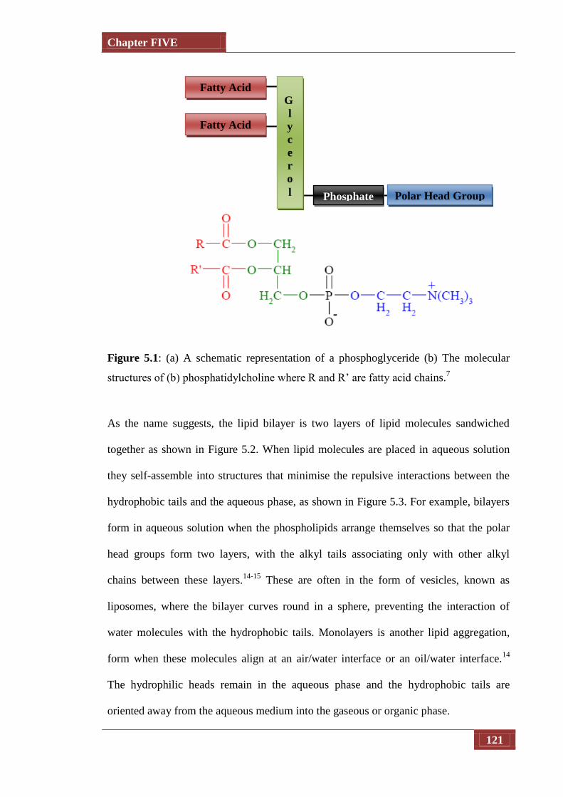
Chapter FIVE
121
Figure 5.1: (a) A schematic representation of a phosphoglyceride (b) The molecular
structures of (b) phosphatidylcholine where R and R’ are fatty acid chains.7
As the name suggests, the lipid bilayer is two layers of lipid molecules sandwiched
together as shown in Figure 5.2. When lipid molecules are placed in aqueous solution
they self-assemble into structures that minimise the repulsive interactions between the
hydrophobic tails and the aqueous phase, as shown in Figure 5.3. For example, bilayers
form in aqueous solution when the phospholipids arrange themselves so that the polar
head groups form two layers, with the alkyl tails associating only with other alkyl
chains between these layers.14-15
These are often in the form of vesicles, known as
liposomes, where the bilayer curves round in a sphere, preventing the interaction of
water molecules with the hydrophobic tails. Monolayers is another lipid aggregation,
form when these molecules align at an air/water interface or an oil/water interface.14
The hydrophilic heads remain in the aqueous phase and the hydrophobic tails are
oriented away from the aqueous medium into the gaseous or organic phase.
G
l
y
c
e
r
o
l
Fatty Acid
Phosphate Polar Head Group
Fatty Acid
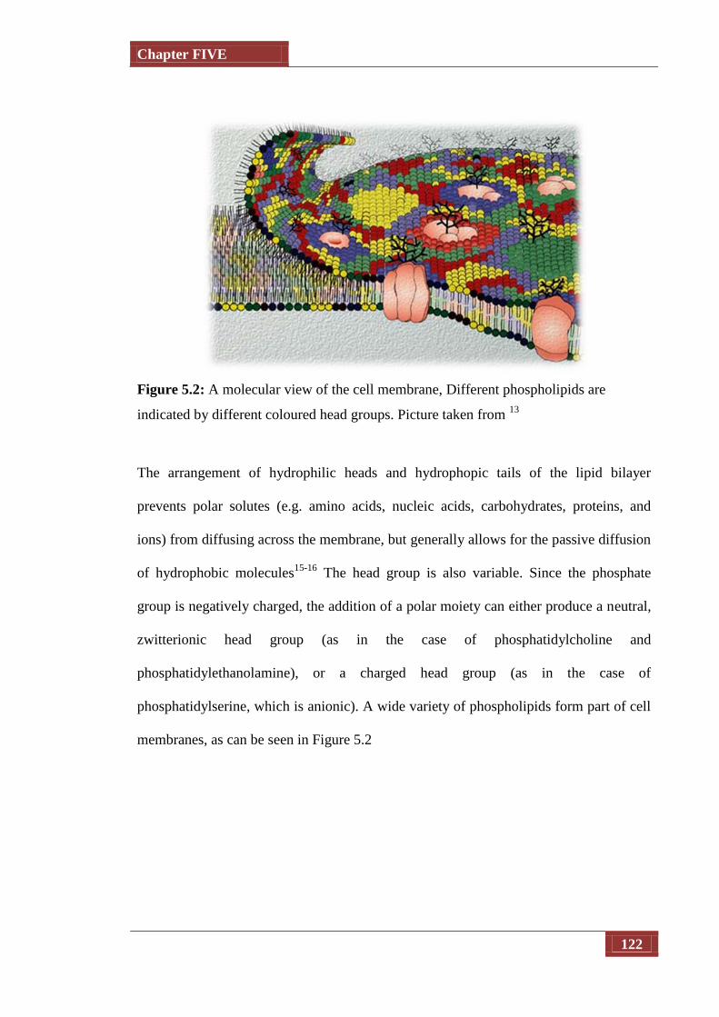
Chapter FIVE
122
Figure 5.2: A molecular view of the cell membrane, Different phospholipids are
indicated by different coloured head groups. Picture taken from 13
The arrangement of hydrophilic heads and hydrophopic tails of the lipid bilayer
prevents polar solutes (e.g. amino acids, nucleic acids, carbohydrates, proteins, and
ions) from diffusing across the membrane, but generally allows for the passive diffusion
of hydrophobic molecules15-16
The head group is also variable. Since the phosphate
group is negatively charged, the addition of a polar moiety can either produce a neutral,
zwitterionic head group (as in the case of phosphatidylcholine and
phosphatidylethanolamine), or a charged head group (as in the case of
phosphatidylserine, which is anionic). A wide variety of phospholipids form part of cell
membranes, as can be seen in Figure 5.2
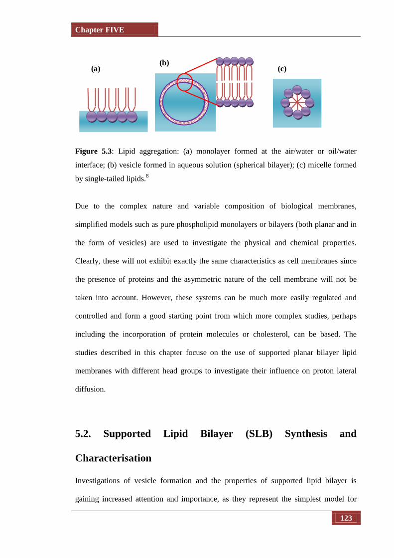
Chapter FIVE
123
Figure 5.3: Lipid aggregation: (a) monolayer formed at the air/water or oil/water
interface; (b) vesicle formed in aqueous solution (spherical bilayer); (c) micelle formed
by single-tailed lipids.8
Due to the complex nature and variable composition of biological membranes,
simplified models such as pure phospholipid monolayers or bilayers (both planar and in
the form of vesicles) are used to investigate the physical and chemical properties.
Clearly, these will not exhibit exactly the same characteristics as cell membranes since
the presence of proteins and the asymmetric nature of the cell membrane will not be
taken into account. However, these systems can be much more easily regulated and
controlled and form a good starting point from which more complex studies, perhaps
including the incorporation of protein molecules or cholesterol, can be based. The
studies described in this chapter focuse on the use of supported planar bilayer lipid
membranes with different head groups to investigate their influence on proton lateral
diffusion.
5.2. Supported Lipid Bilayer (SLB) Synthesis and
Characterisation
Investigations of vesicle formation and the properties of supported lipid bilayer is
gaining increased attention and importance, as they represent the simplest model for
(a) (b)
(c)

Chapter FIVE
124
studying biological processes and characteristics of cell membranes. Studies carried out
on planar bilayer formation have established many procedures to obtain either mono- or
bilayers assemblies. These procedures involve the “brush” technique, the “dipping”
technique17
and the “patch clamp” method18
for unsupported bilayer formation. The
most popular methods used for supported lipid bilayer formation are Langmuir-
Blodgett/Langmuir-Schaeffer19-20
and the vesicles fusion techniques. The fluidity of the
solid supported system is maintained by trapping a water layer (10-20 Å) between the
substrate and the SLB.5,21
The principal method forming SLBs is the vesicle fusion method (which this study
focuses on). Under certain conditions, small unilamellar vesicles (SUVs) of
phospholipids in solution may adsorb on the surface of a solid substrate and
subsequently rupture (either spontaneously or after reaching a critical surface coverage).
The interest in this method arises from its simplicity and because it is fairly
straightforward to integrate membrane proteins into the bilayers by preparing
proteoliposomes.3,6,22
However, the drawback of this method is its high delicacy, since
the size and charge of the vesicles, as well as the charge and morphology of the surface,
has great influence on this process due to the electrostatic interactions.23-24
The pH of
the buffer and the temperature also has a huge effect on the process.22
If the conditions
are not correct, the vesicles may adsorb but not rupture leaving a layer of intact
vesicles.25
Considering electrolyte effects, and the ionic strength of the solution, it has
been established that the presence of divalent cations in the buffer solution such as
calcium or magnesium in very low concentration (ca 2 mM) has an enormous
importance and can effectively induce bilayer formation. There are a number of ways to
form solutions of SUV including multilaminar extrusion through porous polycarbonate

Chapter FIVE
125
membrane at high pressure,26-27
as well as the sonication and ultracentrifugation of
aqueous lipids suspensions.28-29
Other commonly used methods of forming SLBs include the Langmuir-Blodgett (LB)
and Langmuir-Schaeffer (LS) techniques.30
In LB technique, a monolayer is formed at
the air/water interface of a Langmuir Trough, by spreading a lipid solution on it. The
deposition of the multilayer (or even bilayers) on the substrate is carried out by
successively pulling and immersing the substrate up and down vertically through the
monolayer.31
It is also possible to adsorb vesicles to a monolayer created using the
Langmuir-Blodgett technique.32
In the LS technique, the solid substrate is lowered
parallel to the liquid surface to touch the monolayer. These two techniques (LB and LS)
allow the formation of asymmetric bilayers and thus the investigation of the lipid
structure in the top and bottom leaflets; as well as examination of the complex
behaviour of the excess surface area as a function of the composition in two-component
bilayers. Less commonly used bilayer formation techniques include spin coating33-34
and
air bubble collapse.
Various techniques have been used to study and follow SLB formation, and a
combination of more than one method in the study gives better understanding of the
formation mechanism, such as surface plasmon resonance (SPR)35-36
, ellipsometry,37
fluorescence,23,25,38
attenuated total reflectance infrared spectroscopy,30
and quartz
crystal microbalance with dissipation (QCM-D).39-41
One method of forming a lipid
bilayer on a flat support, such as silica, is to apply lipid vesicles to the surface. When
the lipid vesicles come in contact with the SiO2-coated QCM-D or SPR quartz sensor
crystal surface or the silica prism, they first adsorb to the surface as intact vesicles.

Chapter FIVE
126
Once a sufficiently high surface coverage is reached they spontaneously transform into
a bilayer.42
Many techniques have been used to investigate bilayers after their
formation. Fluorescence recovery after photobleaching (FRAP) has been used
extensively to study the mobility and fluidity of the bilayers;32,36
spatially resolved mass
spectrometry to determine lipid distribution in the bilayers;33
AFM to investigate the
topology of the bilayers as well as identifying specific domains in the lipids patches;34,43
spectroscopic methods are also used such as neutron reflectivity,44
X-ray scattering45
and Raman spectroscopy.46
Herein, tapping mode AFM was used to visualize supported
bilayers formed on coverslips.47
5.3. Modification of Surfaces by Ultrathin Films
Ultrathin organic films have gained a lot of interest due to their use in many application
areas, such as composites, catalysis, microelectronics,48
integrated optics, sensors,
friction reducing coating and surface orientation layers.49
Three common methods are
used in the formation of supported thin films on a solid substrate: the Langmuir-
Blodgett technique (see section 5.2 above), chemisorption and self-assembly processes.
Chemisorption implements an adsorption method driven by a chemical reaction at the
surface of interest: the interaction between the surface, and the generated species creates
either ionic or covalent bonds between. While powerful, this shows various drawbacks,
such as the need of the reaction to achieve 100% yield to maintain full coverage in each
layer. Some species do not permit the assembly of high numbered multilayers and so
this method is restricted to limited numbers of organics.49-50
The self-assembly process which was firstly developed by Decher et al,49
this technique
has gained increasing attention and interest due to its simplicity and straightforward

Chapter FIVE
127
formation of the layer with no need for covalent bonds formation or monolayers
transfer, as it only involves adsorption from solution. Multilayers are fabricated by
sequential anionic-cationic polyelectrolyte addition to the substrate, the mechanism
depending on the electrostatic interaction between the species and the substrate surface,
which provides the driving force for the build-up of the multilayer, and guarantees full
coverage of the required compound as the repulsive force between similar charges
prevents any contamination in the layer;51
another advantage is the ability to insert
different materials in the assembled layers such as proteins, biopolymers, virus particles
or inorganic colloids.48
The two polymers studied in this work, poly-l-lysine (PLL) and poly-l-glutamic acids
(PGA) (Figure 5.4), have a lot of applications in various areas such as pharmaceutical
therapy, fuel cells, and biosensors. As well as finding applications in the
aforementioned technologies, polypeptide multilayer films have found a wealth of
applications in medicine for example as polypeptide microcapsules for drug delivery52
or for anti-microbial protection.53
Thus, many studies have been carried out to
understand their properties and characteristics, especially their immobilization and
interaction with protons in aqueous solutions54-55
.
Figure 5.4 General molecular formula of PLL (left) and PGA (right).
O
C
N
H
OH H n

Chapter FIVE
128
5.4. Proton Lateral Diffusion
The movement of protons from source to sink sites is receiving increasing interest due
to its crucial role in bioenergetic processes in the cell membrane, as well as
photosynthesis in green plants, production of electricity in a fuel cell, electrochemical
sensors, and electrochemical reactors56
. In biological systems, the processes of proton
transfer in membranes attract much attention, since hydrogen ions are involved directly
in the processes of energy transformation in membrane in mitochondria, chloroplasts
and bacteria. Proton translocation causes a pH-gradient that controls bioenergetic
processes which couples electron transfer and synthesis of most common free-energy
carrier in the biosphere adenosine triphosphate (ATP), as first suggested by Mitchell’s
chemiosmotic57-61
or other energy requiring processes.62
ATP, which provides the
energy for most chemical reactions in the cells, is generated when an electrochemical
proton gradient exists across the inner membrane. The gradient consists of two
components: a difference in hydrogen ion concentration, or pH, and a difference in
electric potential; the two together form ‘protonmotive force’. A membrane-bound
enzyme, ATP synthesis, provides a channel for protons to move down this gradient,
generating an electrical potential which drives the synthesis of ATP in another part of
the enzyme. This is carried out by trans-membrane proteins e.g. bacteriorhodopsin and
cytochrome oxidase, which function as highly efficient proton pumps.63
Since the proposal of the chemiosmotic theory,63-65
there has been a continuing debate
about how protons that have been pumped across membrane reach another membrane
protein that utilizes the established of pH gradient. Also, how do protons produced by
proton generators get to proton consumers, both located on the same side of the
membrane? Two competing modes for proton transfer have been proposed, one pathway
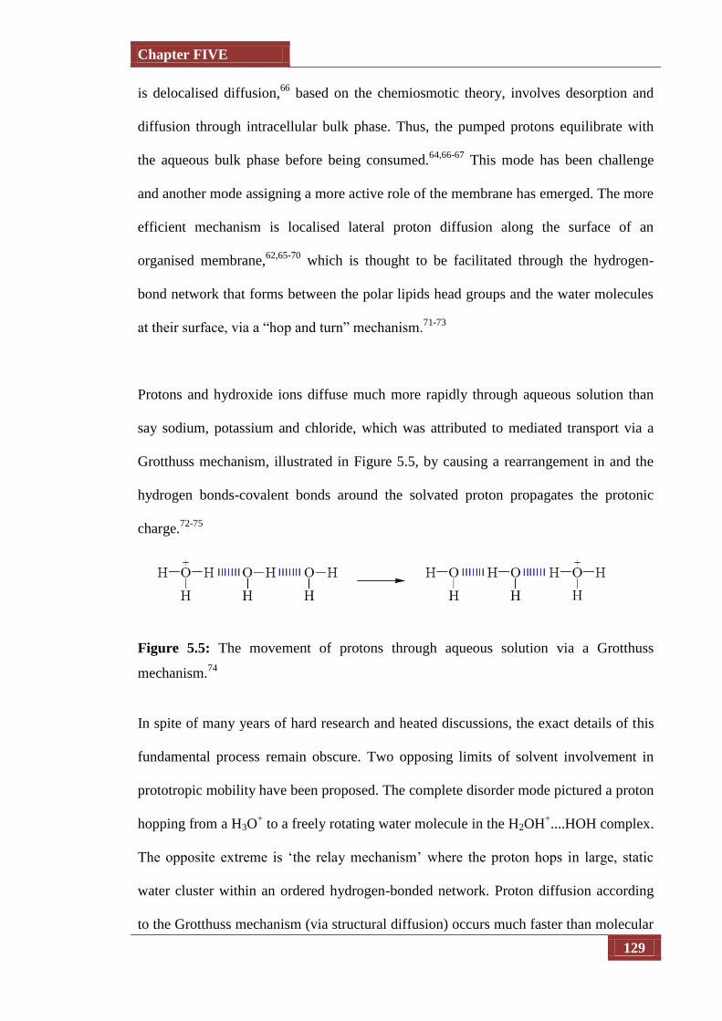
Chapter FIVE
129
is delocalised diffusion,66
based on the chemiosmotic theory, involves desorption and
diffusion through intracellular bulk phase. Thus, the pumped protons equilibrate with
the aqueous bulk phase before being consumed.64,66-67
This mode has been challenge
and another mode assigning a more active role of the membrane has emerged. The more
efficient mechanism is localised lateral proton diffusion along the surface of an
organised membrane,62,65-70
which is thought to be facilitated through the hydrogen-
bond network that forms between the polar lipids head groups and the water molecules
at their surface, via a “hop and turn” mechanism.71-73
Protons and hydroxide ions diffuse much more rapidly through aqueous solution than
say sodium, potassium and chloride, which was attributed to mediated transport via a
Grotthuss mechanism, illustrated in Figure 5.5, by causing a rearrangement in and the
hydrogen bonds-covalent bonds around the solvated proton propagates the protonic
charge.72-75
Figure 5.5: The movement of protons through aqueous solution via a Grotthuss
mechanism.74
In spite of many years of hard research and heated discussions, the exact details of this
fundamental process remain obscure. Two opposing limits of solvent involvement in
prototropic mobility have been proposed. The complete disorder mode pictured a proton
hopping from a H3O+ to a freely rotating water molecule in the H2OH
+....HOH complex.
The opposite extreme is ‘the relay mechanism’ where the proton hops in large, static
water cluster within an ordered hydrogen-bonded network. Proton diffusion according
to the Grotthuss mechanism (via structural diffusion) occurs much faster than molecular

Chapter FIVE
130
diffusion of an acidic carrier (e.g. H3O+) because it is uncoupled from the self-diffusion
of its mass.75
Measuring the rate of such process proved to be difficult with
conventional techniques,76
in addition different experimental techniques did not provide
consistent results. This variation has caused great debate about the insufficiencies of the
methods used77
with criticism being aimed mainly at deficiencies in the methods used to
obtain the data.
Several studies of lateral proton diffusion have been conducted at phospholipid
monolayers spread at the air/water interface, purple membrane, bilayer lipid membrane
and small unilaminar vesicles.72-73
Initial studies by Teissié have reported high values
for the lateral proton diffusion coefficient (at least 20 times that in aqueous
solution),67,78-79
by measuring fluorescence intensity changes of pH-sensitive
fluorophores within Langmuir monolayer at distances over centimetre length scales
from a mechanically stirred compartment where acid was injected. While further studies
reported that the diffusion was simply facilitated; arguments about these results claimed
that convection may contribute to the high rates obtained.75
Using this method, it was
suggested that protons are conducted predominantly by lateral diffusion in mixed
phospholipid, monolayers,80
and at protein films.81-82
The methodology was the subject
of strong criticism, not least because of the long distances and time over which
measurements were made, with arguments of using a magnetic stirrer, introducing
additional convective effects. Many theoretical and experimental investigations both
supported and refuted this result. Indeed, contradictory data were obtained in laser pulse
studies in vesicles and flash spectrophotometry on thylakoids, identify a retardation of
severalfold comparing to bulk aqueous solution.83-84

Chapter FIVE
131
Nevertheless, fast migration of protons along membranes has been observed in purple
membrane compared to transfer into the bulk.69,85
Long-range proton diffusion has also
been observed along lipids 86
and in more recent studies employing the SECM technique
in the induced desorption and feedback modes to study lateral proton diffusion in
monolayers (Langmuir monolayers at water/air interface).87
This approach allows
interfacial dynamics and diffusion to be examined on small distance (micrometers) and
time scale (milliseconds), and the well defined mass transport conditions in the SECM
configuration permits the use of models to interpret the UME response. By the
reduction of protons87
or weak acids88-89
(producing hydrogen) at an UME placed close
to a Langmuir monolayer, deprotonation of the monolayer occurs locally that induces a
proton diffusion gradient in the solution as well as the interface.87-89
. This method
illustrated that the in-plane lateral proton diffusion coefficient depends on the physical
state and acid/base nature of the monolayer and was at most 15% of the magnitude in
bulk solution at acidic monolayers (stearic acid),87
and an order of magnitude lower than
in aqueous bulk solution at (DPPS),88
while it was so small that it could not be detected
at zwitterionic monolayers (DPPC).88
Thus, the proton transfer pathway along the
membrane can be critically dependent on the distance between the source and the sink,
the composition of the solution and the composition of the membrane.
This chapter introduces a new technique directly monitoring lateral proton diffusion at
both surfaces modified with polyelectrolyte films and phospholipid bilayers with
different head group. The technique combines the successful aspects of SECM with the
use of fluorescence CLSM to measure pH changes at the bilayer surface in real time.
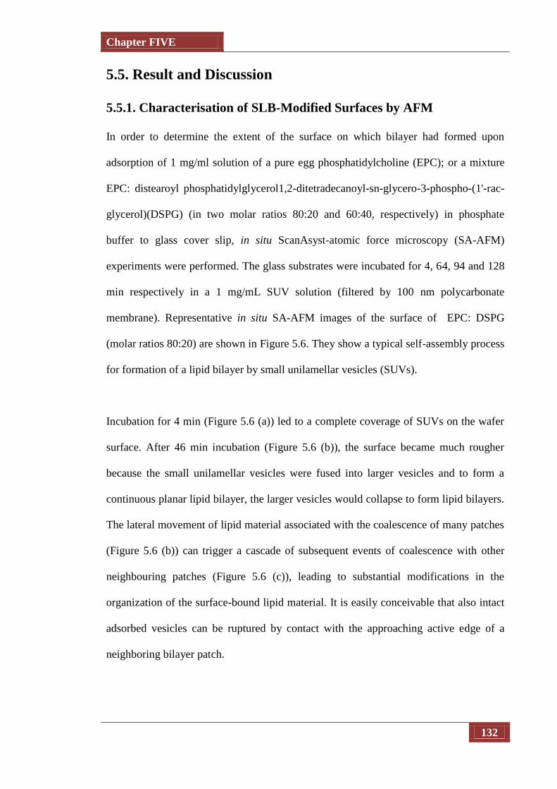
Chapter FIVE
132
5.5. Result and Discussion
5.5.1. Characterisation of SLB-Modified Surfaces by AFM
In order to determine the extent of the surface on which bilayer had formed upon
adsorption of 1 mg/ml solution of a pure egg phosphatidylcholine (EPC); or a mixture
EPC: distearoyl phosphatidylglycerol1,2-ditetradecanoyl-sn-glycero-3-phospho-(1'-rac-
glycerol)(DSPG) (in two molar ratios 80:20 and 60:40, respectively) in phosphate
buffer to glass cover slip, in situ ScanAsyst-atomic force microscopy (SA-AFM)
experiments were performed. The glass substrates were incubated for 4, 64, 94 and 128
min respectively in a 1 mg/mL SUV solution (filtered by 100 nm polycarbonate
membrane). Representative in situ SA-AFM images of the surface of EPC: DSPG
(molar ratios 80:20) are shown in Figure 5.6. They show a typical self-assembly process
for formation of a lipid bilayer by small unilamellar vesicles (SUVs).
Incubation for 4 min (Figure 5.6 (a)) led to a complete coverage of SUVs on the wafer
surface. After 46 min incubation (Figure 5.6 (b)), the surface became much rougher
because the small unilamellar vesicles were fused into larger vesicles and to form a
continuous planar lipid bilayer, the larger vesicles would collapse to form lipid bilayers.
The lateral movement of lipid material associated with the coalescence of many patches
(Figure 5.6 (b)) can trigger a cascade of subsequent events of coalescence with other
neighbouring patches (Figure 5.6 (c)), leading to substantial modifications in the
organization of the surface-bound lipid material. It is easily conceivable that also intact
adsorbed vesicles can be ruptured by contact with the approaching active edge of a
neighboring bilayer patch.
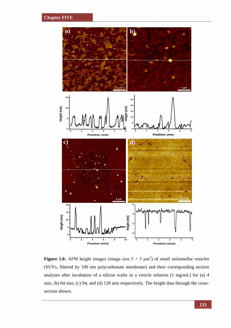
Chapter FIVE
133
Figure 5.6: AFM height images (image size 5 × 5 μm2) of small unilamellar vesicles
(SUVs, filtered by 100 nm polycarbonate membrane) and their corresponding section
analyses after incubation of a silicon wafer in a vesicle solution (1 mg/mL) for (a) 4
min, (b) 64 min, (c) 94, and (d) 128 min respectively. The height data through the cross-
section shown.
0 1 2 3 4 50
5
10
15
Hei
gh
t (n
m)
Position (mm)
0 1 2 3 4 50
5
10
15
20
25
Hei
gh
t (n
m)
Position (mm)
0 1 2 3 4 5
0
2
4
6
Hei
gh
t (n
m)
Position (mm) 0 2 4 6 8 10
0
5
10
15
20
Hei
gh
t (n
m)
Position (mm)
a) b)
c) d)
Chapter FIVE
134
The corresponding cross section profile presents a larger vesicle and also vesicles’
rupturing to form bilayer patches. Due to the fusion of adjacent vesicles or bilayer
patches, the bilayer area became bigger and the constant height of 5 nm90
indicated they
were extended flat bilayers. Bilayer patches coalesced with increasing vesicle exposure
time as shown in Figure 5.7 (b), (c) and (d). Finally, after 128 min a continuous planar
film was formed in Figure 5.7(d), and it entirely covered the substrate surface. From
these AFM images, a conclusion can be drawn for the formation of SLBs: first the small
unilamellar vesicles were adsorbed intact onto the substrate, and then they fused
together into bigger vesicles and finally the bigger vesicles ruptured to a planar
continuous bilayer.
5.5.2. Measurement of proton diffusion at modified surfaces
The studies herein on proton lateral diffusion used an extension of the method employed
in chapters 4. The experimental details are outlined in Chapter 2, section 2.3.2. A UME
was positioned close to the modified surfaces and used to alter the pH of the sub phase,
via galvanostatically oxidising water to produce protons (Chapter 4, Equation 4.2). The
resulting lateral flux of protons along the surface was monitored in real time, by
imaging the change in light intensity by CLSM. A spatio-temporal fluorescence map
showing interfacial proton dispersion was produced, allowing surface effect on
diffusion to be identified. A schematic representation of the method is shown in Figure
5.7.
To validate the method qualitatively, CLSM imaging of proton dispersion in an aqueous
solution of disodium fluorescein was carried out, close to PLL as inert surface and PLG
as proton sink surface. In effect the electrostatic properties of the surface were charged
Chapter FIVE
135
facilitating, the study of electrostatic interactions at positively and negatively charge
surfaces. In this situation, the flux of protons produced at PLL by the electrode reaction
could be used as controlled substrate, as described later, and compared to different
active surfaces.
Figure 5.7: Schematic of the arrangement for SECM-CLSM studies of lateral proton
diffusion, using the electrolysis of water for proton generation.
A range of small currents from 0.5 nA to 2 nA was applied to the UME and the
resulting spatio-temporal images collected. Three typical images, captured during
application of 0.5 nA, 1 nA and 2 nA next to PLL surfaces, are shown in Figure 5.8.
The images clearly show the time at which the current was applied and the decrease in
fluorescence at the interface, as the oxidation of water causes the proton concentration
to rise. Each CLSM image was constructed from the numerical data, light intensity in
arbitrary units (1 – 250) and distance (μm), collected from every line scanned. The time
for a single line scan of length 228 m (was selected across the centre of the electrode
surface, as illustrated schematically in Chapter 2 Figure 2.13), was 2 ms and 2048 lines
H+ H+ H+ H+ H+H+H+H+H+H+
H+ H+ H+ H+ H+H+H+H+H+H+
H+
H+ H
+
Glass cover slip
Modifications of the
surface with PLL,
PGA, or SLB
25 µm Pt UME
Line scanned across
the UME

Chapter FIVE
136
were recorded. Plots of light intensity as a function of distance along the interface could
be studied.
Figure 5.8: Spatio-temporal fluorescence CLSM images of proton dispersion at a PLL
layer. Current applied: (a) 0.5 nA, (b) 1 nA and (c) 2 nA.
The sharp drop in light intensity, following the applied current, occurs at the electrode
edge where the pH is suddenly decreased when protons are produced from the oxidation
of water. The fluorescence intensity then rises steadily with distance away from the
electrode, reflecting the pH profile that has been established in the small volume of
solution between the electrode and the PLL interface. At the longer times following the
applied current, the region of lower light intensity extends further away from the edge
of the electrode indicating the diffusion of protons through the solution. The radius of
the fluorescence profile was found to increase as the applied current was increased to 2
nA since the current controls the flux of protons away from the electrode surface. For
relatively small currents (for example, 0.5 nA in Figure 5.8(a)), the fluorescence did not
spread to the edge of the UME, rather it was localized around the centre. Clearly,
0
1
0.
5
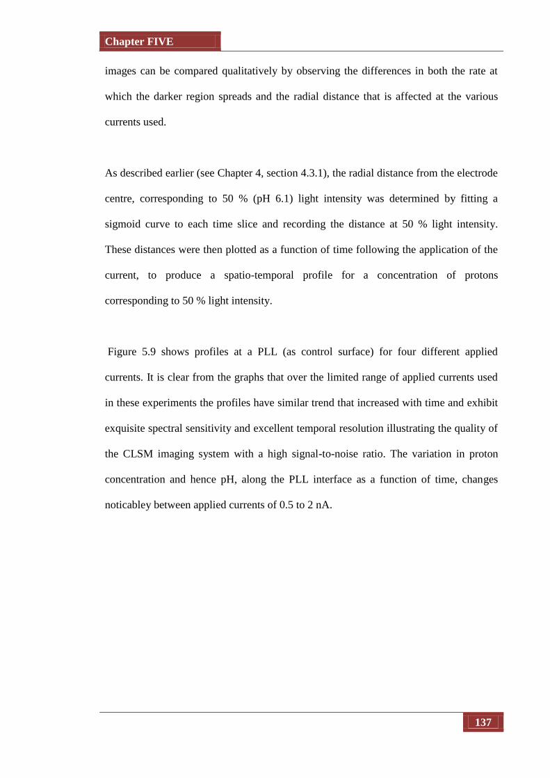
Chapter FIVE
137
images can be compared qualitatively by observing the differences in both the rate at
which the darker region spreads and the radial distance that is affected at the various
currents used.
As described earlier (see Chapter 4, section 4.3.1), the radial distance from the electrode
centre, corresponding to 50 % (pH 6.1) light intensity was determined by fitting a
sigmoid curve to each time slice and recording the distance at 50 % light intensity.
These distances were then plotted as a function of time following the application of the
current, to produce a spatio-temporal profile for a concentration of protons
corresponding to 50 % light intensity.
Figure 5.9 shows profiles at a PLL (as control surface) for four different applied
currents. It is clear from the graphs that over the limited range of applied currents used
in these experiments the profiles have similar trend that increased with time and exhibit
exquisite spectral sensitivity and excellent temporal resolution illustrating the quality of
the CLSM imaging system with a high signal-to-noise ratio. The variation in proton
concentration and hence pH, along the PLL interface as a function of time, changes
noticabley between applied currents of 0.5 to 2 nA.
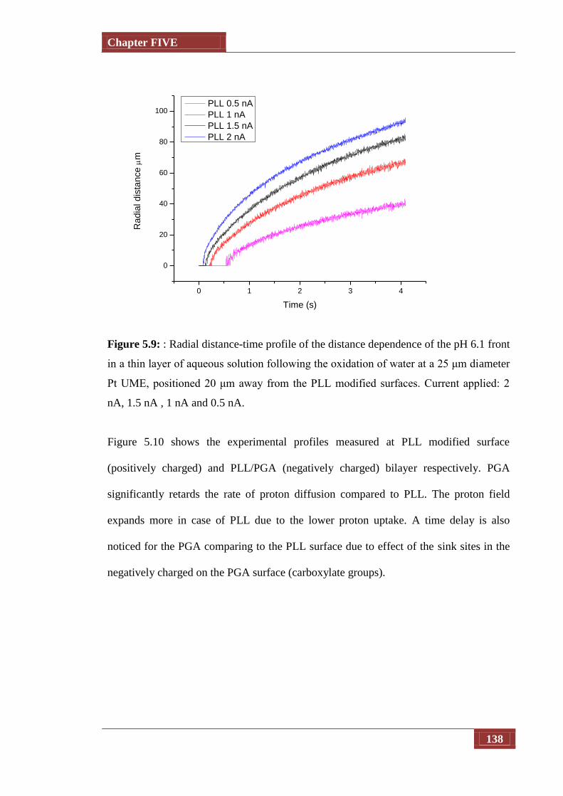
Chapter FIVE
138
0 1 2 3 4
0
20
40
60
80
100
Ra
dia
l d
ista
nce
m
Time (s)
PLL 0.5 nA
PLL 1 nA
PLL 1.5 nA
PLL 2 nA
Figure 5.9: : Radial distance-time profile of the distance dependence of the pH 6.1 front
in a thin layer of aqueous solution following the oxidation of water at a 25 μm diameter
Pt UME, positioned 20 μm away from the PLL modified surfaces. Current applied: 2
nA, 1.5 nA , 1 nA and 0.5 nA.
Figure 5.10 shows the experimental profiles measured at PLL modified surface
(positively charged) and PLL/PGA (negatively charged) bilayer respectively. PGA
significantly retards the rate of proton diffusion compared to PLL. The proton field
expands more in case of PLL due to the lower proton uptake. A time delay is also
noticed for the PGA comparing to the PLL surface due to effect of the sink sites in the
negatively charged on the PGA surface (carboxylate groups).

Chapter FIVE
139
0 1 2 3 4
0
20
40
60
80
100
Dis
tan
ce
(m
)
Time (s)
PGA 2 nA
PLL 2 nA
Figure 5.10: Radial distance-time profile dependence of the pH 6.1 front in a thin layer
of aqueous solution following the oxidation of water at a 25 μm diameter Pt UME,
positioned 20 μm above the PLL (red line), PGA (black line). Current applied: 2 nA.
Proton diffusion at Phospholipids bilayer
Lateral proton diffusion at phospholipid bilayers was explored by changing the lipid
composition. Three different phospholipid systems were investigated: the zwitterionic,
egg phosphatidylcholine (EPC); and a mixture of the acidic, distearoyl
phosphatidylglycerol1,2-ditetradecanoyl-sn-glycero-3-phospho-(1'-rac-glycerol)(DSPG)
with EPC in different molar ratios (20:80 and 40:60, respectively). The natural lipid
extract Egg EPC has a zwitterionic headgroup where a negative charge (from the O- in a
phosphate group) and a positive charge (from the N+ in an amino group) giving the head
an overall neutral charge.91
The lateral protons diffusion along planar bilayers
investigation was carried by applying a range of anodic currents from 0.5 nA to 2 nA to
the UME positioned close to the bilayer, and the resulting spatio-temporal images
collected. A schematic representation of the method is shown in Figure 5.11.
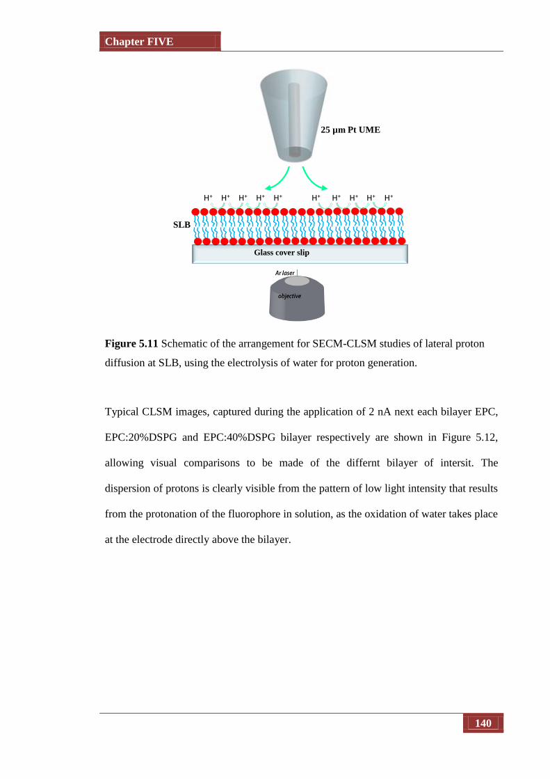
Chapter FIVE
140
Figure 5.11 Schematic of the arrangement for SECM-CLSM studies of lateral proton
diffusion at SLB, using the electrolysis of water for proton generation.
Typical CLSM images, captured during the application of 2 nA next each bilayer EPC,
EPC:20%DSPG and EPC:40%DSPG bilayer respectively are shown in Figure 5.12,
allowing visual comparisons to be made of the differnt bilayer of intersit. The
dispersion of protons is clearly visible from the pattern of low light intensity that results
from the protonation of the fluorophore in solution, as the oxidation of water takes place
at the electrode directly above the bilayer.
H+ H+ H+ H+ H+H+H+H+H+H+
Glass cover slip
25 µm Pt UME
SLB
Chapter FIVE
141
Figure 5.12: Spatio-temporal fluorescence CLSM images of proton dispersion at (a)
EPC, (b) EPC:20%DSPG and (c) EPC:40%DSPG bilayer. Current applied 2 nA. The
scale bar represents 50 m.
Figure 5.13 shows the experimental profiles measured at a EPC and EPC:20%DSPG
and EPC:40%DSPG bilayers respectively, at different currents, compared to the
controls PLL, which assumes that proton dispersion is simply by hindered diffusion
through solution and PGA as proton sink surface. Shown in Figure 5.13 (a) are the
variation of proton diffusion front at pH 6.1 (and hence pH) as a function of time for a 2
nA current showing the inherent differences between the different surfaces with
different chemical and electrostatic properties. The consistency of the data across these
modified surfaces and for a range of currents provides further evidence of the sensitivity
(in terms of both spatial and temporal resolution) of CLSM as a technique for probing
proton diffusion, which allowed the study of these exceptionally fast processes in situ
and in real time.
1
0
0.
5
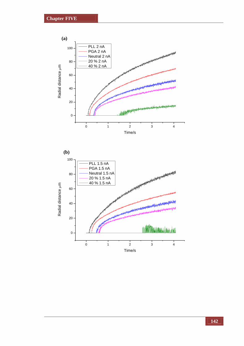
Chapter FIVE
142
0 1 2 3 4
0
20
40
60
80
100
Ra
dia
l d
ista
nce
m
Time/s
PLL 2 nA
PGA 2 nA
Neutral 2 nA
20 % 2 nA
40 % 2 nA
0 1 2 3 4
0
20
40
60
80
100
Ra
dia
l d
ista
nce
m
Time/s
PLL 1.5 nA
PGA 1.5 nA
Neutral 1.5 nA
20 % 1.5 nA
40 % 1.5 nA
(a)
(b)

Chapter FIVE
143
0 1 2 3 4
-10
0
10
20
30
40
50
60
70
Ra
dia
l d
ista
nce
m
Time/s
PLL 1 nA
PGA 1 nA
Neutral 1 nA
20 % 1 nA
40 % 1 nA
Figure 5.13: Radial distance-time profiles of the distance dependence of the pH 6.1
front in a thin layer of aqueous solution following the oxidation of water at a 25 μm
diameter Pt UME, positioned 20 μm above PLL (black line), PLG (pink line), EPC(blue
line), EPC:20%DSPG (red line) and EPC:40%DSPG (green line). Current applied: (a) 2
nA , (b) 1.5 nA and (c) 1 nA.
As can be seen, the nature of the surface strongly modulated the proton dispersion
profiles obtained. For the PLL modified surface the proton is the most rapid and
extensive: PLL thus behaves as an inert surface as discussed earlier. In all others cases,
the presence of active surfaces in the front of PLG and the phospholipid bilayers with
different head group significantly retards the rate and extent of proton diffusion. This is
most apparent for all of the lipid bilayers, where the final distance (at 4 s) is less than
half of that observed for the PLL surface.
Interestingly, at short times, within 2 s, for all applied current, there is a time delay that
increase with increasing concentration of the negatively charged sites in the surface.
This is diagnostic of these sites acting as sink sites towards the flux of proton generated.
(c)
Chapter FIVE
144
The concentration of these sites has similar influence on the rate and extent of the
proton dispersion. The rate of diffusion slows down and the distance that the
concentration profile reaches is dependent on the composition of the surface. The rate of
proton diffusion was slower at EPC:20%DSPG and EPC:40%DSPG respectively than at
EPC bilayer; however, when currents below 2 nA were applied to the UME above
EPC:40%DSPG bilayer, the light intensity dropped over a distance was not seen to
spread in a radial direction; thus no proton profile was observed.
It can be seen also from the graphs that the proton diffusion expands more in case of
lower proton uptake as in case of zwitterionic EPC than EPC:20%DSPG and
EPC:40%DSPG bilayer respectively, as expected for proton at more negative charge
surfaces. Interestingly, proton diffusion expands more in case of PLG more than both
bilayers, DSPG and EPC. The consistency of the data across different modified surfaces
and for a range of currents provides further evidence of the sensitivity (in terms of both
spatial and temporal resolution) of CLSM as a technique for probing proton diffusion,
which allowed the study of these exceptionally fast processes in situ and in real time.
The head groups of PGA, DSPG and EPC, indicating their charges (Figure 5.14); PGA
has 2 carboxyl groups with an apparent pKa = of 4.4, both lipid DSPG and EPC have a
phosphate group with a pKa of ca. 2.2 However, DSPG has a negative charge due to the
deprotonated phosphate group but EPC has no net charge due to the presence of an
amino group with a pKa of ca. 9.7. As protons are produced at the electrode close to the
bilayer surface, the phosphate group on the DSPG bilayer will protonate more rapidly
than the phosphate group on EPC because it is less acidic (larger pKa value). It is

Chapter FIVE
145
suggested that the greater availability of protonation sites at the membrane will retain
protons at the surface and prevent spreading in solution.
Figure 5.14: Structures of the head groups of (a) DSPG, (b) EPC and (c) PLG.
5.7. Conclusions
This chapter has described a new approach for studying proton diffusion at modified
surfaces. In the experiments described herein, electrochemical methods were used as a
means to induce surface processes which could then be followed in real-time and in situ
using CLSM. The ability to form a supported lipid bilayer on the glass surface was
demonstrated, and more importantly, the possibility of studying proton diffusion at
modified surfaces was investigated. SECM has been successfully combined with CLSM
to image proton diffusion at the surface of phospholipid bilayers using a Pt UME for
local water oxidation, at the surface of thin films (PLL, PLL/PGA, EPC and DSPG)
deposited on a solid substrate surface (glass). This powerful technique has established
(c)
(b)
(a)
O
OH O C
N
H
Chapter FIVE
146
well that proton diffusion near the PLL modified surface (positively charged) has a
higher rate compared to the PGA surface (negatively charged); this was explained by
the ability of the carboxylic groups to protonate at the beginning of this process, which
would cause a time delay for the progress of the 50% intensity front (pH 6.1). EPC was
also found to have a lower rate of proton diffusion than DSPG (negatively charged) that
can be explained by the acid-base character of the phospholipids.
There are a number of factors can control the rate of lateral proton diffusion, which
include the nature of the lipid, membrane fluidity and the buffering capacity and ionic
strength of the solution. The value of the anodic current applied to the UME is another
critical factor that controls the experimental observations. Due to the saturation of the
substrate surface (active sites), there is a delay in the time to reach the steady-state
current which increases as the current became lower. This has been well notified at
active surface in comparison to inert surface. The ability to form a SLB on glass
substrate and to monitor the proton diffusion on modified surfaces in situ and in real
time, expands the applicability of CLSM to the study lateral proton diffusion in a
biologically relevant environment. Thus, the well-defined delivery methods employed
in these experiments described now need to be quantitatively modelled to further
understand the reaction mechanisms and to resolve what is happening.

Chapter FIVE
147
5.7. Conclusions
This chapter has described a new approach for studying proton diffusion at modified
surfaces. In the experiments described herein, electrochemical methods were used as a
means to induce surface processes which could then be followed in real-time and in situ
using CLSM. The ability to form a supported lipid bilayer on the glass surface was
demonstrated, and more importantly, the possibility of studying proton diffusion at
modified surfaces was investigated. SECM has been successfully combined with CLSM
to image proton diffusion at the surface of phospholipid bilayers using a Pt UME for
local water oxidation, at the surface of thin films (PLL, PLL/PGA, EPC and DSPG)
deposited on a solid substrate surface (glass). This powerful technique has established
well that proton diffusion near the PLL modified surface (positively charged) has a
higher rate compared to the PGA surface (negatively charged); this was explained by
the ability of the carboxylic groups to protonate at the beginning of this process, which
would cause a time delay for the progress of the 50% intensity front (pH 6.1). EPC was
also found to have a lower rate of proton diffusion than DSPG (negatively charged) that
can be explained by the acid-base character of the phospholipids.
There are a number of factors that can control the rate of lateral proton diffusion, which
include the nature of the lipid, membrane fluidity and the buffering capacity and ionic
strength of the solution. The value of the anodic current applied to the UME is another
critical factor that controls the experimental observations. Due to the saturation of the
substrate surface (active sites), there is a delay in the time to reach the steady-state
current which increases as the current became lower. This has been well notified at
active surface in comparison to inert surface. The ability to form a SLB on glass
substrate and to monitor the proton diffusion on modified surfaces in situ and in real

Chapter FIVE
148
time, expands the applicability of CLSM to the study lateral proton diffusion in a
biologically relevant environment. Thus, the well-defined delivery methods employed
in these experiments described now need to be quantitatively modelled to further
understand the reaction mechanisms and to resolve what is happening.

Chapter FIVE
149
5.8. References
(1) Fiedler, S.; Broecker, J.; Keller, S. Cellular and Molecular Life Sciences 2010, 67,
1779.
(2) McConnell, H. M.; Watts, T. H.; Weis, R. M.; Brian, A. A. Biochimica Et
Biophysica Acta 1986, 864, 95.
(3) Perez, T. D.; Nelson, W. J.; Boxer, S. G.; Kam, L. Langmuir 2005, 21, 11963.
(4) Kam, L. C. Journal of Structural Biology 2009, 168, 3.
(5) Castellana, E. T.; Cremer, P. S. Surface Science Reports 2006, 61, 429.
(6) O'Rourke, B. In Annual Review of Physiology 2007; Vol. 69, p 19.
(7) Jain, M., K. Introduction to Biological Membranes; 1ed ed.; John Wiley & Sons:
USA, 1938.
(8) Jain, M., K., The Bimolecular Lipid Membranes; 1ed ed.; Van Nostrand Reinhold
Company,: USA, 1972.
(9) Stryer, L. Biochemistry; 4th ed.; W. H. Freeman and Company: New York, USA,
1995.
(10) Karnovsky, M. J.; Kleinfeld, A. M.; Hoover, R. L.; Klausner, R. D. Journal of
Cell Biology 1982, 94, 1.
(11) Cullis, P. R.; Dekruijff, B. Current Contents/Life Sciences 1992, 11.
(12) Cullis, P. R.; Dekruijff, B. Biochimica Et Biophysica Acta 1979, 559, 399.
(13) Edidin, M. Nature Reviews Molecular Cell Biology 2003, 4, 414.
(14) Gunstone, F. D. H., J. L.; Padley, F. B. The Lipid Handbook;; Chapman and
Hall:: London, 1986.
(15) Orbach, E.; Finkelstein, A. Journal of General Physiology 1980, 75, 427.
(16) Grime, J. M. A.; Edwards, M. A.; Rudd, N. C.; Unwin, P. R. Proceedings of the
National Academy of Sciences of the United States of America 2008, 105, 14277.
(17) Tien, H. T. Bilayer Lipid Membranes (BLM). Theory and Practice; Marcel
Dekker: New York, 1974.
(18) Suarezisla, B. A.; Wan, K.; Lindstrom, J.; Montal, M. Biochemistry 1983, 22,
2319.
(19) Dominska, M.; Krysinski, P.; Blanchard, G. J. Langmuir 2008, 24, 8785.
(20) Nikolov, V.; Lin, J.; Merzlyakov, M.; Hristova, K.; Searson, P. C. Langmuir
2007, 23, 13040.
(21) Cho, N.-J.; Frank, C. W.; Kasemo, B.; Hook, F. Nature Protocols 2010, 5, 1096.
(22) Seantier, B.; Breffa, C.; Felix, O.; Decher, G. Journal of Physical Chemistry B
2005, 109, 21755.
(23) Nollert, P.; Kiefer, H.; Jahnig, F. Biophysical Journal 1995, 69, 1447.
(24) Radler, J.; Strey, H.; Sackmann, E. Langmuir 1995, 11, 4539.
(25) Reuter, M.; Schwieger, C.; Meister, A.; Karlsson, G.; Blume, A. Biophysical
Chemistry 2009, 144, 27.
(26) Lapinski, M. M.; Castro-Forero, A.; Greiner, A. J.; Ofoli, R. Y.; Blanchard, G. J.
Langmuir 2007, 23, 11677.
(27) Frisken, B. J.; Asman, C.; Patty, P. J. Langmuir 2000, 16, 928.
(28) Maulucci, G.; De Spirito, M.; Arcovito, G.; Boffi, F.; Castellano, A. C.; Briganti,
G. Biophysical Journal 2005, 88, 3545.
(29) Barenholz, Y.; Gibbes, D.; Litman, B. J.; Goll, J.; Thompson, T. E.; Carlson, F. D.
Biochemistry 1977, 16, 2806.
(30) Olivieri, M. P.; Wollman, R. M.; Hurley, M. I.; Swartz, M. F. Journal of Adhesion
2010, 86, 111.
(31) Binks, B. P. Advances in Colloid and Interface Science 1991, 34, 343.

Chapter FIVE
150
(32) Ma, C.; Srinivasan, M. P.; Waring, A. J.; Lehrer, R. I.; Longo, M. L.; Stroeve, P.
Colloids and Surfaces B-Biointerfaces 2003, 28, 319.
(33) Kraft, M. L.; Weber, P. K.; Longo, M. L.; Hutcheon, I. D.; Boxer, S. G. Science
2006, 313, 1948.
(34) Zhang, L. F.; Spurlin, T. A.; Gewirth, A. A.; Granick, S. Journal of Physical
Chemistry B 2006, 110, 33.
(35) Papo, N.; Shai, Y. Biochemistry 2003, 42, 458.
(36) Munro, J. C.; Frank, C. W. Langmuir 2004, 20, 10567.
(37) Benes, M.; Billy, D.; Benda, A.; Speijer, H.; Hof, M.; Hermens, W. T. Langmuir
2004, 20, 10129.
(38) Barman, H.; Walch, M.; Latinovic-Golic, S.; Dumrese, C.; Dolder, M.; Groscurth,
P.; Ziegler, U. Journal of Membrane Biology 2006, 212, 29.
(39) Richter, R.; Mukhopadhyay, A.; Brisson, A. Biophysical Journal 2003, 85, 3035.
(40) Richter, R. P.; Brisson, A. R. Biophysical Journal 2005, 88, 3422.
(41) Roberts, G. G. Langmuir-Blodgett films; illustrated ed.; Plenum Press: New York,
1990.
(42) Keller, C. A.; Kasemo, B. Biophysical Journal 1998, 75, 1397.
(43) Burns, A. R. Langmuir 2003, 19, 8358.
(44) Kucerka, N.; Nagle, J. F.; Sachs, J. N.; Feller, S. E.; Pencer, J.; Jackson, A.;
Katsaras, J. Biophysical Journal 2008, 95, 2356.
(45) Generosi, J.; Margaritondo, G.; Sanghera, J. S.; Aggarwal, I. D.; Tolk, N. H.;
Piston, D. W.; Castellano, A. C.; Cricenti, A. Applied Physics Letters 2006, 89.
(46) Lee, C. S.; Bain, C. D. Biochimica Et Biophysica Acta-Biomembranes 2005,
1711, 59.
(47) Mager, M. D.; Almquist, B.; Melosh, N. A. Langmuir 2008, 24, 12734.
(48) Schmitt, J.; Decher, G.; Dressick, W. J.; Brandow, S. L.; Geer, R. E.; Shashidhar,
R.; Calvert, J. M. Advanced Materials 1997, 9, 61.
(49) Decher, G.; Hong, J. D.; Schmitt, J. Thin Solid Films 1992, 210, 831.
(50) Lee, H.; Kepley, L. J.; Hong, H. G.; Akhter, S.; Mallouk, T. E. Journal of
Physical Chemistry 1988, 92, 2597.
(51) Bertrand, P.; Jonas, A.; Laschewsky, A.; Legras, R. Macromolecular Rapid
Communications 2000, 21, 319.
(52) Leguen, E.; Chassepot, A.; Decher, G.; Schaaf, P.; Voegel, J.-C.; Jessel, N.
Biomolecular Engineering 2007, 24, 33.
(53) Boulmedais, F.; Frisch, B.; Etienne, O.; Lavalle, P.; Picart, C.; Ogier, J.; Voegel,
J. C.; Schaaf, P.; Egles, C. Biomaterials 2004, 25, 2003.
(54) Hamano, Y.; Nicchu, I.; Shimizu, T.; Onji, Y.; Hiraki, J.; Takagi, H. Applied
Microbiology and Biotechnology 2007, 76, 873.
(55) Pasut, G.; Veronese, F. M. Progress in Polymer Science 2007, 32, 933.
(56) Kreuer, K.-D. Chemistry of Materials 1996, 8, 610.
(57) Gennis, R. B. Biomembranes: Molecular Structure and Function New York,
1989.
(58) Medvedev, E. S.; Stuchebrukhov, A. A. Journal of Physics-Condensed Matter
2011, 23.
(59) Mulkidjanian, A. Y.; Heberle, J.; Cherepanov, D. A. Biochimica Et Biophysica
Acta-Bioenergetics 2006, 1757, 913.
(60) Agmon, N.; Gutman, M. Nat Chem 2011, 3, 840.
(61) Serowy, S.; Saparov, S. M.; Antonenko, Y. N.; Kozlovsky, W.; Hagen, V.; Pohl,
P. Biophysical Journal 2003, 84, 1031.
Chapter FIVE
151
(62) Georgievskii, Y.; Medvedev, E. S.; Stuchebrukhov, A. A. Biophysical Journal
2002, 82, 2833.
(63) Ferguson, S. J. Current Biology 1995, 5, 25.
(64) Mitchell, P. Nature 1961, 191, 144.
(65) Heberle, J.; Riesle, J.; Thiedemann, G.; Oesterhelt, D.; Dencher, N. A. Nature
1994, 370, 379.
(66) Antonenko, Y. N.; Kovbasnjuk, O. N.; Yaguzhinsky, L. S. Biochimica Et
Biophysica Acta 1993, 1150, 45.
(67) Prats, M.; Teissie, J.; Tocanne, J. F. Nature 1986, 322, 756.
(68) Kell, D. B. Biochimica Et Biophysica Acta 1979, 549, 55.
(69) Alexiev, U.; Scherrer, P.; Mollaaghababa, R.; Khorana, H. G.; Heyn, M. P.
Biophysical Journal 1995, 68, A321.
(70) Georgievskii, Y.; Medvedev, E. S.; Stuchebrukhov, A. A. Journal of Chemical
Physics 2002, 116, 1692.
(71) Agmon, N. Chem. Phys. Lett. 1995, 244, 456.
(72) Agmon, N. Chemical Physics Letters 1995, 244, 456.
(73) Agmon, N. Abstracts of Papers of the American Chemical Society 1995, 210, 328.
(74) Compton, R. G. S., G. H. W. Electrode Potentials; PressOxford University UK,
1998.
(75) Gutman, M.; Nachliel, E. Biochimica Et Biophysica Acta-Bioenergetics 1995,
1231, 123.
(76) Scherrer, P. Nature 1995, 374, 222.
(77) Sakurai, I.; Suzuki, T.; Sakurai, S. Biochimica Et Biophysica Acta 1989, 985, 101.
(78) Teissie, J.; Prats, M.; Soucaille, P.; Tocanne, J. F. Proceedings of the National
Academy of Sciences of the United States of America 1985, 82, 3217.
(79) Prats, M.; Tocanne, J. F.; Teissie, J. European Journal of Biochemistry 1985, 149,
663.
(80) Gabriel, B.; Prats, M.; Teissie, J. Biochemistry 1991, 30, 9359.
(81) Antonenko, Y. N.; Pohl, P. European Biophysics Journal with Biophysics Letters
2008, 37, 865.
(82) Gabriel, B.; Teissie, J. Proceedings of the National Academy of Sciences of the
United States of America 1996, 93, 14521.
(83) Nachliel, E.; Gutman, M. Journal of the American Chemical Society 1988, 110,
2629.
(84) Gutman, M.; Nachliel, E.; Moshiach, S. Biochemistry 1989, 28, 2936.
(85) Nachliel, E.; Gutman, M.; Kiryati, S.; Dencher, N. A. Proceedings of the National
Academy of Sciences of the United States of America 1996, 93, 10747.
(86) Gabriel, B.; Prats, M.; Teissie, J. Biochimica Et Biophysica Acta-Bioenergetics
1994, 1186, 172.
(87) Slevin, C. J.; Unwin, P. R. Journal of the American Chemical Society 2000, 122,
2597.
(88) Zhang, J.; Unwin, P. R. Journal of the American Chemical Society 2002, 124,
2379.
(89) Zhang, J.; Unwin, P. R. Phys. Chem. Chem. Phys. 2002, 4, 3814.
(90) Reviakine, I.; Brisson, A. Langmuir 2000, 16, 1806.
(91) Notter, R. H. Lung surfactants: basic science and clinical applications; 1st ed.;
CRC Press: New York, 2000; Vol. 149.
(92) Branden, M.; Sanden, T.; Brzezinski, P.; Widengren, J. Proceedings of the
National Academy of Sciences of the United States of America 2006, 103, 19766.

Chapter FIVE
152
(93) Medvedev, E. S.; Stuchebrukhov, A. A. Journal of Mathematical Biology 2006,
52, 209.
(94) Springer, A.; Hagen, V.; Cherepanov, D. A.; Antonenko, Y. N.; Pohl, P.
Proceedings of the National Academy of Sciences of the United States of America
2011, 108, 14461.
(95) Cherepanov, D. A.; Feniouk, B. A.; Junge, W.; Mulkidjanian, A. Y. Biophysical
Journal 2003, 85, 2069.
(96) Smondyrev, A. M.; Voth, G. A. Biophysical Journal 2002, 82, 1460.
(97) Cherepanov, D. A.; Junge, W.; Mulkidjanian, A. Y. Biophysical Journal 2004, 86,
665.
Chapter SIX
153
Conclusion 6
As highlighted in the introduction (chapter 1), this thesis has considered various
experimental techniques and simulation, for describing diffusion in electrochemical
systems and beyond. A key aspect of the thesis has been the quantification of
concentration gradients produced at active surfaces during an electrode reaction with a
wide range of materials. Progress has been made in each area investigated, providing a
foundation for the future. The combination of fluorescence confocal laser scanning
microscopy (CLSM) with electrochemical techniques has allowed such processes to be
visualised and the defining parameters to be determined. Many electrode and interface
processes are accompanied by local changes in pH, and the methodology described in
this thesis could find wider application in quantifying associated pH gradients and in
providing mechanistic information.
Chapter 3 considered the concentration profile of redox reactions adjacent to novel OT-
UMEs comprising ultrathin films of SWNTs. The SWNT films are grown by cCVD on
a single crystal ST-cut quartz substrate. They exhibited both complete transparency and
disc-shaped UME characteristics. In particular, the OT-SWNT-UMEs demonstrated the
attractive properties of small-scale electrodes, e.g., high diffusion rates and good signal-
to-noise, with the ability to probe electrochemical processes optically, from the rear of
the electrode. This enabled optical measurements of the solution, close to the electrode
Chapter SIX
154
surface, without significant interference from absorption or scattering processes. The
electrochemical activity of the UMEs was quantified using CLSM with the temporal
and spatial resolution in the millisecond and micrometer range, respectively. The
investigation involved use of fluorophores which were either redox active (Ru(bpy)32+
oxidation) or had the luminescent properties which were pH sensitive (fluorescein in
oxygen reduction reaction (ORR)). These proof-of-concept experiments broaden the
potential applications of the introduced SWNT disc UMEs as reliable and effective
sensors for broad optical and electrochemical applications. Further developments in OT-
UME fabrication will allow quantitative analysis of reaction dynamics at a greatly
enhanced level. Initial improvements in the OT-UME design by using thinner quartz
substrates, both fused quartz and single crystal, would enable use of higher
magnification objectives with increased resolution capabilities which should allow the
more faithful measurement of concentration profiles. With the suggested improvement,
several classes of experiments could be carried out such as electrogenerated
chemiluminescence studies of species providing intense luminescence. The technique
would be particularly useful in detecting defects in electrodes and active sites on
heterogeneous electrode surfaces.
An important outcome of the studies herein is the ability to assess the effectiveness of
inhibitors on enamel dissolution that could be expanded to include many types of
substrate. The use of CLSM combined scanning electrochemical microscopy (SECM)
provides a very powerful tool, which enables the visualisation of the proton gradient
established near the surface of an UME, thus permitting the tracking of proton
movement on various substrates located nearby. This provided an analytical method
with high spatial and temporal resolution permitting sub-second analysis of treatment
Chapter SIX
155
effects on enamel substrates. Localised dissolution of dental enamel has been achieved
by the application of a proton flux to the enamel surface from a UME positioned in
close proximity to the enamel, in aqueous solution. It has been shown that fluoride and
zinc as dissolution inhibitors cause changes in the morphology of pH profile that forms
on treated enamel compared to untreated enamel due to their barrier effect. Fluoride
treatment of enamel provides an initial barrier to proton attack with a rate constant
similar to that of zinc treated enamel, but this barrier only lasted for approximately one
second before returning to a rate comparable to that of untreated enamel. Experimental
observations were quantified by solving the diffusion equations numerically. The
experimental data were compared to the finite element model, which allowed rate
constants of dissolution to be assigned for different surface treatments at different
proton fluxes controlled by the applied current. Simulated pH profiles were found to be
in close agreement with the experimental CLSM pH profiles, including inhibitor effects
at short and long time scales. Based on these data, CLSM-SECM appears to be
particularly powerful and it would be possible to assess many complex inhibitors of acid
erosion with this method.
A new approach has been developed and tested to examining proton uptake and lateral
proton diffusion at thin films surfaces (polymers, lipid bilayers and related systems), to
further extend the capabilities of the method developed using CLSM combined with
SECM to directly visualise proton fluxes at modified surfaces. The methodology was
verified by application to galvanostatic water reduction as a well characterised system.
For studies of proton diffusion, silica surfaces were modified by multilayer assemblies
of poly-L-lysine (PLL) and poly-L-glutamic acid (PLG) thereby changing the
electrostatic properties of the surface and facilitating the study of different electrostatic

Chapter SIX
156
interactions. The resulting surface charge is positive in the case of PLL and negative in
the case of a PLL/PLG bilayer. Both PLL and PGA functionalised interfaces were
studied as controls for comparison to the lipid bilayers. The different surfaces had a
significant impact on the extent of proton uptake. In the future phospholipids with
hydrocarbon chains of different lengths or degrees of unsaturation, could be used to
examine the effects of packing and organisation of the bilayer on proton uptake. The
fluidity of the bilayer may also have an effect on proton diffusion and this could be
investigated by incorporating cholesterol into the phospholipid bilayer. The
incorporation of protein channels such as bacterial photosynthetic membrane proteins,
light-harvesting complex 2 (LH2), and light-harvesting core complex (LH1-RC) could
also be the subject of future work. This can be achieved by introducing spacers between
the membrane and the substrate using polymer cushions and pillars as the typical
supported lipid bilayer is separated from the surface of the substrate by a 1-2 nm of
water layer, which has been believed this water layer cannot provide enough space for
large protuberant domains of membrane proteins. The high resolution of the technique
would allow visualisation of the diffusion profile through labelling the bilayer itself
with a pH sensitive fluorophore in addition to the one that exists in the bulk solution.
Simulation model will now need to be developed to describe the proton gradient
established at the UME surface in the presence of an inert and active substrate in order
to obtain quantitative data and deduce uptake extent and lateral proton diffusion.

Appendix
157
Appendix A
Attached to the thesis there are a series of movies related to experiments described in
chapter 3, 4 and 5.
Movie 1: Oxidation of 10 mM Ru(bpy)32+
in 0.1 M NaCl at a 50 µm diameter disc-
shaped OT-SWNTs-UME
Movie 2: Proton gradient following the oxidation of water in 8 μM fluorescein solution
with 0.1 M potassium nitrate at a 25 μm diameter Pt UME. Current applied: 20 nA.
Movie 3: Proton gradient following the oxidation of water in 8 μM fluorescein solution
with 0.1 M potassium nitrate at a 25 μm diameter Pt UME, positioned 20 μm away from
glass surfaces. Current applied: 20 nA
Movie 4: Proton gradient following the oxidation of water in 8 μM fluorescein solution
with 0.1 M potassium nitrate at a 25 μm diameter Pt UME, positioned 20 μm away from
enamel surface. Current applied: 20 nA
Movie 5: Proton gradient following the oxidation of water in 8 μM fluorescein solution
with 0.1 M potassium nitrate at a 25 μm diameter Pt UME, positioned 20 μm away from
modified surface. Current applied: 20 nA

Appendix
158