University of Southampton Research Repository ePrints Soton20PhD%20thesis%20... · algoritmanin...
260
University of Southampton Research Repository ePrints Soton Copyright © and Moral Rights for this thesis are retained by the author and/or other copyright owners. A copy can be downloaded for personal non-commercial research or study, without prior permission or charge. This thesis cannot be reproduced or quoted extensively from without first obtaining permission in writing from the copyright holder/s. The content must not be changed in any way or sold commercially in any format or medium without the formal permission of the copyright holders. When referring to this work, full bibliographic details including the author, title, awarding institution and date of the thesis must be given e.g. AUTHOR (year of submission) "Full thesis title", University of Southampton, name of the University School or Department, PhD Thesis, pagination http://eprints.soton.ac.uk
Transcript of University of Southampton Research Repository ePrints Soton20PhD%20thesis%20... · algoritmanin...

University of Southampton Research Repository
ePrints Soton
Copyright © and Moral Rights for this thesis are retained by the author and/or other copyright owners. A copy can be downloaded for personal non-commercial research or study, without prior permission or charge. This thesis cannot be reproduced or quoted extensively from without first obtaining permission in writing from the copyright holder/s. The content must not be changed in any way or sold commercially in any format or medium without the formal permission of the copyright holders.
When referring to this work, full bibliographic details including the author, title, awarding institution and date of the thesis must be given e.g.
AUTHOR (year of submission) "Full thesis title", University of Southampton, name of the University School or Department, PhD Thesis, pagination
http://eprints.soton.ac.uk

UNIVERSITY of SOUTHAMPTON
FACULTY OF BUSINESS AND LAW
SOUTHAMPTON BUSINESS SCHOOL
Heterogeneous Location- and
Pollution-Routing Problems
by
Cagrı Koc
Thesis for the degree of Doctor of Philosophy
September 2015

UNIVERSITY of SOUTHAMPTON
FACULTY OF BUSINESS AND LAW
SOUTHAMPTON BUSINESS SCHOOL
Heterogeneous Location- and
Pollution-Routing Problems
by
Cagrı Koc
Main supervisor: Professor Tolga Bektas
Supervisor: Dr. Ola Jabali
Supervisor: Professor Gilbert Laporte
Internal Examiner: Professor Chris Potts
External Examiner: Professor Tom Van Woensel
Thesis for the degree of Doctor of Philosophy in Management Science
September 2015

UNIVERSITY of SOUTHAMPTON
Abstract
FACULTY OF BUSINESS AND LAW
SOUTHAMPTON BUSINESS SCHOOL
Doctor of Philosophy in Management Science
Heterogeneous Location- and Pollution-Routing Problems
by Cagrı Koc
This thesis introduces and studies new classes of heterogeneous vehicle routing problems
with or without location and pollution considerations. It develops powerful evolutionary
and adaptive large neighborhood search based metaheuristics capable of solving a wide
variety of such problems with suitable enhancements, and provides several important
managerial insights. It is structured into five main chapters. After the introduction
presented in Chapter 1, Chapter 2 classifies and reviews the relevant literature on het-
erogeneous vehicle routing problems, and presents a comparative analysis of the available
metaheuristic algorithms for these problems. Chapter 3 describes a hybrid evolutionary
algorithm for four variants of heterogeneous fleet vehicle routing problems with time
windows. The algorithm successfully combines several metaheuristics and introduces a
number of new advanced efficient procedures. Extensive computational experiments on
benchmark instances show that the algorithm is highly competitive with state-of-the art
methods for the three variants. New benchmark results on the fourth problem are also
presented. In Chapter 4, the thesis introduces the fleet size and mix location-routing
problem with time windows (FSMLRPTW) which extends the classical location-routing
problem by considering a heterogeneous fleet and time windows. The main objective of
the FSMLRPTW is to minimize the sum of depot cost, vehicle fixed cost and routing
cost. The thesis presents integer programming formulations for the FSMLRPTW, along
with a family of valid inequalities and an algorithm based on adaptation of the hybrid
evolutionary metaheuristic. The strengths of the formulations are evaluated with respect
to their ability to yield optimal solutions. Extensive computational experiments on new
benchmark instances show that the algorithm is highly effective. Chapter 5 introduces

ii
the fleet size and mix pollution-routing problem (FSMPRP) which extends the previ-
ously studied pollution-routing problem (PRP) by considering a heterogeneous vehicle
fleet. The main objective is to minimize the sum of vehicle fixed costs and routing cost,
where the latter can be defined with respect to the cost of fuel and CO2 emissions, and
driver cost. An adaptation of the hybrid evolutionary algorithm is successfully applied
to a large pool of realistic PRP and FSMPRP benchmark instances, where new best so-
lutions are obtained for the former. Several analyses are conducted to shed light on the
trade-offs between various performance indicators. The benefit of using a heterogeneous
fleet over a homogeneous one is demonstrated. In Chapter 6, the thesis investigates
the combined impact of depot location, fleet composition and routing decisions on vehi-
cle emissions in urban freight distribution characterized by several speed limits, where
goods need to be delivered from a depot to customers located in different speed zones.
To solve the problem, an adaptive large neighborhood search algorithm is successfully
applied to a large pool of new benchmark instances. Extensive analyses are conducted
to quantify the effect of various problem parameters, such as depot cost and location,
customer distribution and fleet composition on key performance indicators, including
fuel consumption, emissions and operational costs. The results illustrate the benefits of
locating depots located in suburban areas rather than in the city centre and of using a
heterogeneous fleet over a homogeneous one. The conclusions, presented in Chapter 7,
summarize the results of the thesis, provide limitations of this work, as well as future
research directions.
Keywords. Operational research; combinatorial optimisation; logistics; city logistics;
transportation; vehicle routing; location-routing; heterogeneous fleet; fleet size and mix;
fuel consumption; CO2 emissions; sustainability; evolutionary metaheuristic; adaptive
large neighborhood search.

UNIVERSITY of SOUTHAMPTON
Ozet
FACULTY OF BUSINESS AND LAW
SOUTHAMPTON BUSINESS SCHOOL
Doktora, Yoneylem Arastırması
Heterojen Yer Secimi- ve Cevre Kirliligi-Rotalama
Problemleri
by Cagrı Koc
Bu calısmada, heterojen arac rotalama problemlerinin yer secimi ve cevre kirliligi ozellikle-
rinin oldugu ve olmadıgı yeni cesitleri tanımlanmıs, oldukca guclu, etkili ve bircok prob-
lem cesidini basarıyla cozebilen evrime dayalı ve uyarlanabilir buyuk komsuluk arama
metasezgiselleri gelistirilmis, ve cesitli idari bakıs acıları saglanmıstır. Calısma bes
ana bolumden olusmaktadır. Birinci bolumde sunulan giris kısmının ardından, ikinci
bolumde heterojen arac rotalama problemleri ile ilgili literatur taranmıs ve sınıflandırılmıs,
devamında bu problemler icin literaturde onerilmis metasezgisel algoritmalar karsılastırıl-
mıstır. Ucuncu bolumde, heterojen filolu ve zaman pencereli arac rotalama problem-
lerinin dort farklı cesidi icin evrime dayalı karma bir algoritma gelistirilmistir. Onerilen
algoritma cesitli metasezgiselleri biraraya getirmekle birlikte yeni ve etkili yontemler
icermektedir. Test problemleri uzerinde gerceklestirilen genis kapsamlı deneysel calısmalar,
gelistirilen algoritmanin literaturde bu tur problemler icin gelistirilen en etkili yontemlerle
oldukca sıkı bir sekilde rekabet edebildigini gostermistir. Dorduncu bolumde, bilesik
yer secimi ve rotalama problemleminin genellestirilmis bir cesidi olan heterojen filolu
ve zaman pencereli yer secimi-rotalama problemi tanımlanmıs ve incelenmistir. Bu
problemin temel amacı depo, arac ve rotalama maliyetleri toplamını enkucuklemektir.
Problemin cozumu icin, gecerli esitsizliklerle kuvvetlendirilmis tamsayılı programlama
formulasyonları onerilmis, ayrıca karma evrime dayalı algoritmanın bir baska cesidi
gelistirilmistir. Onerilen formulasyonların etkinlikleri, eniyi cozume ulasma yetenek-
leri acısından deneyler ile degerlendirilmistir. Yeni uretilen test problemleri uzerinde
gerceklestirilen genis kapsamlı deneyler, gelistirilen metasezgisel algoritmanın oldukca

iv
basarılı oldugunu gostermistir. Besinci bolumde, bilesik cevre kirliligi ve rotalama prob-
leminin genellestirilmis bir cesidi olan heterojen filolu cevre kirliligi rotalama problemi
tanımlanmıstır. Bu problemin temel amacı, arac, rotalama, yakıt, CO2 salınımı ile
surucu maliyetleri toplamını enkucuklemektir. Problemin cozumu icin evrime dayalı
algoritmanin baska bir cesidi gelistirilmistir. Hem gozonune alınan problem, hem de
problemin homojen filolu cesidi icin, genis kapsamlı gercekci test problemleri uzerinde
deneyler gerceklestirilmistir. Deneyler sonucunda problemin homojen filolu cesidi icin
literaturde varolan test problemleri uzerinde yeni en iyi cozum degerleri elde edilmistir.
Ayrıca problem parametrelerinin cesitli performans gostergeleri uzerindeki etkilerine ısık
tutmak icin ek analizler gerceklestirilmis, bu analizler sonucunda homojen arac filosu
yerine heterojen arac filosu kullanımının faydaları acıkca ortaya konulmustur. Altıncı
bolumde, cesitli hız bolgelerine ayrılmıs olan sehirici yuk tasımacılıgındaki depo yerinin,
arac filosunun ve rotalama kararlarının, arac CO2 salınımı uzerindeki butunlesik etkisi
analiz edilmistir. Problemde, urunlerin sehir icinde bulunan depolardan, yine sehir icinde
yer alan musterilere ulastırılması amaclanmaktadır. Problemi cozmek icin, uyarlanabilir
bir buyuk komsuluk arama metasezgiseli gelistirilmis ve cesitli yeni test problemleri
uzerinde etkinligi incelenmistir. Depo yeri ve maliyeti, musteri dagılımı ve heterojen
arac filosu gibi problem parametrelerinin, yakıt tuketimi, CO2 salınımı ve operasyonel
maliyetler gibi performans gostergeleri uzerindeki degisimlerinin etkisini analiz etmek
icin, genis kapsamlı deneyler gerceklestirilmistir. Elde edilen sonuclarda, depoların sehir
ici yerine banliyolere yerlestirilmesinin ve homojen arac filosu yerine heterojen arac
filosu kullanımının faydaları numerik sonuclarla gosterilmistir. Yedinci bolumde, tez
calısmasında elde edilen sonuclar kısaca ozetlenmis, calısmanın sınırları ortaya konulmus
ve gelecek calısmalar icin cesitli oneriler sunulmustur.
Anahtar kelimeler. Yoneylem arastırması; kesikli eniyileme; lojistik; sehir lojistigi;
ulastırma; arac rotalama; yer secimi-rotalama; heterojen filo; yakıt tuketimi; CO2 salınımı;
surdurebilirlik; evrime dayalı metasezgisel; uyarlanabilir buyuk komsuluk arama metasez-
giseli.

Contents
Abstract i
Ozet iii
Contents v
List of Figures ix
List of Tables x
Declaration of Authorship xii
Acknowledgements xiii
List of Abbreviations xvi
1 Introduction 1
1.1 Context of the Research Problems . . . . . . . . . . . . . . . . . . . . . . 2
1.2 Illustration: The FedEx Global Distribution Network . . . . . . . . . . . . 4
1.3 Context of the Methodology . . . . . . . . . . . . . . . . . . . . . . . . . . 5
1.4 General Research Contributions . . . . . . . . . . . . . . . . . . . . . . . . 6
1.5 Specific Objectives . . . . . . . . . . . . . . . . . . . . . . . . . . . . . . . 7
2 Thirty Years of Heterogeneous Vehicle Routing 10
2.1 Introduction . . . . . . . . . . . . . . . . . . . . . . . . . . . . . . . . . . . 11
2.2 Classification of the Heterogeneous Vehicle Routing Problem . . . . . . . 12
2.2.1 Problem definition and classification . . . . . . . . . . . . . . . . . 12
2.2.1.1 Objectives . . . . . . . . . . . . . . . . . . . . . . . . . . 13
2.2.1.2 Time windows . . . . . . . . . . . . . . . . . . . . . . . . 13
2.2.1.3 Other variants . . . . . . . . . . . . . . . . . . . . . . . . 14
2.2.2 Mathematical formulations . . . . . . . . . . . . . . . . . . . . . . 14
2.2.2.1 Single-commodity flow formulation . . . . . . . . . . . . . 15
2.2.2.2 Two-commodity flow formulation . . . . . . . . . . . . . 16
2.2.2.3 Set partitioning formulation . . . . . . . . . . . . . . . . 17
2.3 The Fleet Size and Mix Vehicle Routing Problem . . . . . . . . . . . . . . 18
2.3.1 Lower bounds and exact algorithms . . . . . . . . . . . . . . . . . 18
2.3.2 Continuous approximation models . . . . . . . . . . . . . . . . . . 20
2.3.3 Heuristics . . . . . . . . . . . . . . . . . . . . . . . . . . . . . . . . 20
2.3.3.1 Population search heuristics . . . . . . . . . . . . . . . . 20
v

Contents vi
2.3.3.2 Tabu search heuristics . . . . . . . . . . . . . . . . . . . . 21
2.3.3.3 Other heuristics . . . . . . . . . . . . . . . . . . . . . . . 22
2.4 The Heterogeneous Fixed Fleet Vehicle Routing Problem . . . . . . . . . 24
2.4.1 Tabu search heuristics . . . . . . . . . . . . . . . . . . . . . . . . . 24
2.4.2 Other heuristics . . . . . . . . . . . . . . . . . . . . . . . . . . . . 24
2.5 The fleet size and mix vehicle routing problem with time windows . . . . 25
2.5.1 Tabu search heuristics . . . . . . . . . . . . . . . . . . . . . . . . . 26
2.5.2 Other heuristics . . . . . . . . . . . . . . . . . . . . . . . . . . . . 26
2.6 Variants and Extensions . . . . . . . . . . . . . . . . . . . . . . . . . . . . 28
2.6.1 The multi-depot HVRP . . . . . . . . . . . . . . . . . . . . . . . . 28
2.6.2 The green HVRP . . . . . . . . . . . . . . . . . . . . . . . . . . . . 31
2.6.3 The HVRP with backhauls . . . . . . . . . . . . . . . . . . . . . . 32
2.6.4 The HVRP with external carriers . . . . . . . . . . . . . . . . . . . 33
2.6.5 The HVRP with container loading . . . . . . . . . . . . . . . . . . 34
2.6.6 The HVRP with split deliveries . . . . . . . . . . . . . . . . . . . . 35
2.6.7 The HVRP with pickup and delivery . . . . . . . . . . . . . . . . . 35
2.6.8 The open HVRP . . . . . . . . . . . . . . . . . . . . . . . . . . . . 36
2.6.9 Other HVRP variants and extensions . . . . . . . . . . . . . . . . 36
2.7 Case Studies . . . . . . . . . . . . . . . . . . . . . . . . . . . . . . . . . . 40
2.8 Summary and Computational Comparisons . . . . . . . . . . . . . . . . . 42
2.8.1 Summary . . . . . . . . . . . . . . . . . . . . . . . . . . . . . . . . 43
2.8.2 Metaheuristics computational comparisons . . . . . . . . . . . . . 44
2.8.2.1 Comparison of recent metaheuristics on the FSM . . . . . 48
2.8.2.2 Comparison of recent metaheuristics on the HF . . . . . 48
2.8.2.3 Comparison of recent metaheuristics on the FSMTW . . 51
2.9 Conclusions and Future Research Directions . . . . . . . . . . . . . . . . . 51
3 A Hybrid Evolutionary Algorithm for Heterogeneous Fleet VehicleRouting Problems with Time Windows 55
3.1 Introduction . . . . . . . . . . . . . . . . . . . . . . . . . . . . . . . . . . . 56
3.2 Description of the Hybrid Evolutionary Algorithm . . . . . . . . . . . . . 59
3.2.1 Overview of the hybrid evolutionary algorithm . . . . . . . . . . . 60
3.2.2 Education . . . . . . . . . . . . . . . . . . . . . . . . . . . . . . . 61
3.2.2.1 Removal operators . . . . . . . . . . . . . . . . . . . . . . 64
3.2.2.2 Insertion operators . . . . . . . . . . . . . . . . . . . . . . 66
3.2.2.3 Adaptive weight adjustment procedure . . . . . . . . . . 66
3.2.3 Initialization . . . . . . . . . . . . . . . . . . . . . . . . . . . . . . 67
3.2.4 Parent selection . . . . . . . . . . . . . . . . . . . . . . . . . . . . . 67
3.2.5 Crossover . . . . . . . . . . . . . . . . . . . . . . . . . . . . . . . . 68
3.2.6 Split algorithm . . . . . . . . . . . . . . . . . . . . . . . . . . . . 69
3.2.7 Intensification . . . . . . . . . . . . . . . . . . . . . . . . . . . . 72
3.2.8 Survivor selection . . . . . . . . . . . . . . . . . . . . . . . . . . . . 72
3.2.9 Diversification . . . . . . . . . . . . . . . . . . . . . . . . . . . . . 73
3.3 Computational Experiments . . . . . . . . . . . . . . . . . . . . . . . . . . 74
3.3.1 Data sets and experimental settings . . . . . . . . . . . . . . . . . 75
3.3.2 Comparative analysis . . . . . . . . . . . . . . . . . . . . . . . . . 76
3.4 Conclusions . . . . . . . . . . . . . . . . . . . . . . . . . . . . . . . . . . . 82

Contents vii
4 The Fleet Size and Mix Location-Routing Problem with Time Win-dows: Formulations and a Heuristic Algorithm 83
4.1 Introduction . . . . . . . . . . . . . . . . . . . . . . . . . . . . . . . . . . . 84
4.2 Formulations for the Fleet Size and Mix Location-Routing Problem withTime Windows . . . . . . . . . . . . . . . . . . . . . . . . . . . . . . . . . 86
4.2.1 Notation and problem definition . . . . . . . . . . . . . . . . . . . 86
4.2.2 Integer programming formulations . . . . . . . . . . . . . . . . . . 87
4.2.3 Valid inequalities . . . . . . . . . . . . . . . . . . . . . . . . . . . . 91
4.3 Description of the Hybrid Evolutionary Search Algorithm . . . . . . . . . 92
4.3.1 Initialization . . . . . . . . . . . . . . . . . . . . . . . . . . . . . 93
4.3.2 Partition . . . . . . . . . . . . . . . . . . . . . . . . . . . . . . . 94
4.3.3 Education . . . . . . . . . . . . . . . . . . . . . . . . . . . . . . . 94
4.3.3.1 Diversification based removal operators . . . . . . . . . . 95
4.3.3.2 Intensification based removal operators . . . . . . . . . . 97
4.3.3.3 Insertion operators . . . . . . . . . . . . . . . . . . . . . . 98
4.3.4 Mutation . . . . . . . . . . . . . . . . . . . . . . . . . . . . . . . 98
4.4 Computational Experiments . . . . . . . . . . . . . . . . . . . . . . . . . . 98
4.4.1 Benchmark instances . . . . . . . . . . . . . . . . . . . . . . . . . . 99
4.4.2 Sensitivity analysis of method components . . . . . . . . . . . . . . 100
4.4.3 Performance of the formulations . . . . . . . . . . . . . . . . . . . 102
4.4.4 Comparative analysis . . . . . . . . . . . . . . . . . . . . . . . . . 105
4.5 Conclusions . . . . . . . . . . . . . . . . . . . . . . . . . . . . . . . . . . . 106
5 The Fleet Size and Mix Pollution-Routing Problem 110
5.1 Introduction . . . . . . . . . . . . . . . . . . . . . . . . . . . . . . . . . . . 111
5.2 Background on Vehicle Types and Characteristics . . . . . . . . . . . . . . 114
5.3 Mathematical Model for the Fleet Size and Mix Pollution-Routing Problem119
5.4 Description of the Hybrid Evolutionary Algorithm . . . . . . . . . . . . . 121
5.4.1 Speed optimization algorithm . . . . . . . . . . . . . . . . . . . . . 123
5.4.2 The Split algorithm with the speed optimization algorithm . . . . 125
5.4.3 Higher Education and Intensification . . . . . . . . . . . . . 125
5.5 Computational Experiments and Analyses . . . . . . . . . . . . . . . . . . 128
5.5.1 Sensitivity analysis on method components . . . . . . . . . . . . . 128
5.5.2 Results on the PRP and on the FSMPRP . . . . . . . . . . . . . . 129
5.5.3 The effect of cost components . . . . . . . . . . . . . . . . . . . . . 132
5.5.4 The effect of the heterogeneous fleet . . . . . . . . . . . . . . . . . 133
5.6 Conclusions . . . . . . . . . . . . . . . . . . . . . . . . . . . . . . . . . . . 137
6 The Impact of Location, Fleet Composition and Routing on Emissionsin Urban Freight Distribution 140
6.1 Introduction . . . . . . . . . . . . . . . . . . . . . . . . . . . . . . . . . . . 141
6.1.1 A brief review of the literature . . . . . . . . . . . . . . . . . . . . 142
6.1.2 Scientific contributions and structure of the paper . . . . . . . . . 145
6.2 General Description of the Problem Setting . . . . . . . . . . . . . . . . . 145
6.2.1 Fuel consumption and CO2 emissions . . . . . . . . . . . . . . . . 146
6.2.2 Vehicle types and characteristics . . . . . . . . . . . . . . . . . . . 147
6.2.3 Speed zones . . . . . . . . . . . . . . . . . . . . . . . . . . . . . . . 149
Contents viii
6.2.4 Network structure . . . . . . . . . . . . . . . . . . . . . . . . . . . 150
6.2.5 Depot costs . . . . . . . . . . . . . . . . . . . . . . . . . . . . . . . 152
6.3 Formal Problem Description and Mathematical Formulation . . . . . . . . 152
6.4 Description of the ALNS Metaheuristic . . . . . . . . . . . . . . . . . . . . 155
6.4.1 Cheapest path calculation . . . . . . . . . . . . . . . . . . . . . . . 156
6.4.2 Overview of the metaheuristic . . . . . . . . . . . . . . . . . . . . . 157
6.5 Computational Experiments and Analyses . . . . . . . . . . . . . . . . . . 160
6.5.1 Results obtained on the test instances . . . . . . . . . . . . . . . . 161
6.5.2 The effect of the various cost components of the objective function 163
6.5.3 The effect of variations in depot and customer locations . . . . . . 165
6.5.4 The effect of variations in depot costs . . . . . . . . . . . . . . . . 171
6.5.5 The effect of fleet composition . . . . . . . . . . . . . . . . . . . . 173
6.6 Conclusions and Managerial Insights . . . . . . . . . . . . . . . . . . . . . 176
7 Conclusions 179
7.1 Overview . . . . . . . . . . . . . . . . . . . . . . . . . . . . . . . . . . . . 180
7.2 Summary of the Main Scientific Contributions . . . . . . . . . . . . . . . . 180
7.3 Research Outputs . . . . . . . . . . . . . . . . . . . . . . . . . . . . . . . . 182
7.4 Limitations of the Research Results . . . . . . . . . . . . . . . . . . . . . . 184
7.5 Future Research Directions . . . . . . . . . . . . . . . . . . . . . . . . . . 185
7.6 Excitement! . . . . . . . . . . . . . . . . . . . . . . . . . . . . . . . . . . . 185
A Supplement to Chapter 2 187
B Supplement to Chapter 3 193
C Supplement to Chapter 4 201
D Supplement to Chapter 5 211
E Supplement to Chapter 6 216
Bibliography 221

List of Figures
1.1 The FedEx global distribution network (FedEx 2015) . . . . . . . . . . . . 5
1.2 A schematic representation of the thesis structure . . . . . . . . . . . . . . 7
2.1 A classification of HVRP variants . . . . . . . . . . . . . . . . . . . . . . . 29
3.1 Illustration of the Education procedure . . . . . . . . . . . . . . . . . . . 62
3.2 Illustration of Ordered Crossover . . . . . . . . . . . . . . . . . . . . 69
3.3 Illustration of procedure Split . . . . . . . . . . . . . . . . . . . . . . . . 71
3.4 Illustration of the diversification stage . . . . . . . . . . . . . . . . . . . . 74
4.1 Illustration of the L-HALNS procedure . . . . . . . . . . . . . . . . . . . 96
5.1 Three vehicle types (MAN 2014a) . . . . . . . . . . . . . . . . . . . . . . . 116
5.2 Illustration of the HALNS procedure . . . . . . . . . . . . . . . . . . . . 126
6.1 Fuel consumption as a function of speed . . . . . . . . . . . . . . . . . . . 149
6.2 Grid city examples (Google Maps 2015) . . . . . . . . . . . . . . . . . . . 151
6.3 Illustration of speed zones . . . . . . . . . . . . . . . . . . . . . . . . . . . 152
6.4 Illustration of the three speed zones . . . . . . . . . . . . . . . . . . . . . 158
6.5 Geographical customer distribution in the benchmark instances . . . . . . 162
ix

List of Tables
2.1 Literature on the FSM . . . . . . . . . . . . . . . . . . . . . . . . . . . . . 45
2.2 Literature on the HF . . . . . . . . . . . . . . . . . . . . . . . . . . . . . . 46
2.3 Literature on the FSM and the HF . . . . . . . . . . . . . . . . . . . . . . 47
2.4 Average comparison of recent metaheuristics on the FSM . . . . . . . . . 49
2.5 Average comparison of recent metaheuristics on the HF . . . . . . . . . . 50
2.6 Comparison of recent metaheuristics on the FSMTW(T) . . . . . . . . . . 52
2.7 Comparison of recent metaheuristics on the FSMTW(D) . . . . . . . . . . 53
3.1 Average percentage deviations of the solution values found by the HEAfrom best-known solution values with varying np and no . . . . . . . . . . 76
3.2 Average results for FT . . . . . . . . . . . . . . . . . . . . . . . . . . . . . 78
3.3 Average results for FD . . . . . . . . . . . . . . . . . . . . . . . . . . . . . 79
3.4 Results for HT . . . . . . . . . . . . . . . . . . . . . . . . . . . . . . . . . 80
3.5 Results for HD . . . . . . . . . . . . . . . . . . . . . . . . . . . . . . . . . 81
4.1 The intervals for depot capacities . . . . . . . . . . . . . . . . . . . . . . . 100
4.2 Sensitivity analysis experiment setup . . . . . . . . . . . . . . . . . . . . . 100
4.3 Sensitivity analysis of the HESA components . . . . . . . . . . . . . . . . 101
4.4 Average results of the formulations . . . . . . . . . . . . . . . . . . . . . . 103
4.5 Effect of the valid inequalities . . . . . . . . . . . . . . . . . . . . . . . . . 104
4.6 Average results on small-size instances . . . . . . . . . . . . . . . . . . . . 107
4.7 Average results on medium- and large-size instances . . . . . . . . . . . . 108
5.1 Vehicle common parameters . . . . . . . . . . . . . . . . . . . . . . . . . . 115
5.2 Vehicle specific parameters . . . . . . . . . . . . . . . . . . . . . . . . . . 117
5.3 Sensitivity analysis experiment setup . . . . . . . . . . . . . . . . . . . . . 129
5.4 Sensitivity analysis of the HEA++ components . . . . . . . . . . . . . . . 130
5.5 Computational results on the 100-node PRP instances . . . . . . . . . . . 131
5.6 Computational results on the 200-node PRP instances . . . . . . . . . . . 132
5.7 Average results on the FSMPRP instances . . . . . . . . . . . . . . . . . . 132
5.8 The effect of cost components: objective function values . . . . . . . . . . 134
5.9 The effect of cost components: percent deviation from the minimum value 135
5.10 The effect of the speed . . . . . . . . . . . . . . . . . . . . . . . . . . . . . 136
5.11 The effect of using a heterogeneous fleet . . . . . . . . . . . . . . . . . . . 138
5.12 Capacity utilization rates . . . . . . . . . . . . . . . . . . . . . . . . . . . 139
6.1 Vehicle common parameters . . . . . . . . . . . . . . . . . . . . . . . . . . 147
6.2 Vehicle specific parameters . . . . . . . . . . . . . . . . . . . . . . . . . . 148
6.3 Parameters used in the P-L-HALNS . . . . . . . . . . . . . . . . . . . . . 163
x

List of Tables xi
6.4 Average results on the instances . . . . . . . . . . . . . . . . . . . . . . . 164
6.5 The effect of cost components: objective function values. . . . . . . . . . . 166
6.6 The effect of cost components: percent deviation from the minimum value.167
6.7 The effect of variations in depot location. . . . . . . . . . . . . . . . . . . 168
6.8 The effect of variations in customer location. . . . . . . . . . . . . . . . . 170
6.9 The effect of same depot costs on opened depots. . . . . . . . . . . . . . . 172
6.10 The effect of decreasing the depot costs. . . . . . . . . . . . . . . . . . . . 174
6.11 The effect of using a heterogeneous fleet . . . . . . . . . . . . . . . . . . . 175
6.12 Capacity utilization rates . . . . . . . . . . . . . . . . . . . . . . . . . . . 177
A.1 Comparison of recent metaheuristics on the FSM(F,V) . . . . . . . . . . . 188
A.2 Comparison of recent metaheuristics on the FSM(F) . . . . . . . . . . . . 189
A.3 Comparison of recent metaheuristics on the FSM(V) . . . . . . . . . . . . 190
A.4 Comparison of recent metaheuristics on the HF(F,V) . . . . . . . . . . . . 191
A.5 Comparison of recent metaheuristics on the HF(V) . . . . . . . . . . . . . 192
B.1 Sensitivity analyis experiment setup . . . . . . . . . . . . . . . . . . . . . 194
B.2 Sensitivity analyis of the HEA components . . . . . . . . . . . . . . . . . 194
B.3 Number of iterations as a percentage by education operators . . . . . . . 194
B.4 Results for FT for cost structure A . . . . . . . . . . . . . . . . . . . . . . 195
B.5 Results for FT for cost structure B . . . . . . . . . . . . . . . . . . . . . . 196
B.6 Results for FT for cost structure C . . . . . . . . . . . . . . . . . . . . . . 197
B.7 Results for FD for cost structure A . . . . . . . . . . . . . . . . . . . . . . 198
B.8 Results for FD for cost structure B . . . . . . . . . . . . . . . . . . . . . . 199
B.9 Results for FD for cost structure C . . . . . . . . . . . . . . . . . . . . . . 200
C.1 The FSMLRPTW benchmark instances . . . . . . . . . . . . . . . . . . . 202
C.2 Results on the 10-customer instances . . . . . . . . . . . . . . . . . . . . . 203
C.3 Results on the 15-customer instances . . . . . . . . . . . . . . . . . . . . . 204
C.4 Results on the 20-customer instances . . . . . . . . . . . . . . . . . . . . . 205
C.5 Results on the 25-customer instances . . . . . . . . . . . . . . . . . . . . . 206
C.6 Results on the 30-customer instances . . . . . . . . . . . . . . . . . . . . . 207
C.7 Results on the 50-customer instances . . . . . . . . . . . . . . . . . . . . . 208
C.8 Results on the 75-customer instances . . . . . . . . . . . . . . . . . . . . . 209
C.9 Results on the 100-customer instances . . . . . . . . . . . . . . . . . . . . 210
D.1 Computational results on the 75-node FSMPRP instances . . . . . . . . . 212
D.2 Computational results on the 100-node FSMPRP instances . . . . . . . . 213
D.3 Computational results on the 150-node FSMPRP instances . . . . . . . . 214
D.4 Computational results on the 200-node FSMPRP instances . . . . . . . . 215
E.1 Computational results on the 25-customer instances. . . . . . . . . . . . . 217
E.2 Computational results on the 50-customer instances. . . . . . . . . . . . . 218
E.3 Computational results on the 75-customer instances. . . . . . . . . . . . . 219
E.4 Computational results on the 100-customer instances. . . . . . . . . . . . 220

Declaration of Authorship
I, Cagrı Koc, declare that this thesis titled, ’Heterogeneous Location- and Pollution-
Routing Problems’ and the work presented in it are my own. I confirm that:
This work was done wholly or mainly while in candidature for a research degree
at this University.
Where any part of this thesis has previously been submitted for a degree or any
other qualification at this University or any other institution, this has been clearly
stated.
Where I have consulted the published work of others, this is always clearly at-
tributed.
Where I have quoted from the work of others, the source is always given. With
the exception of such quotations, this thesis is entirely my own work.
I have acknowledged all main sources of help.
Where the thesis is based on work done by myself jointly with others, I have made
clear exactly what was done by others and what I have contributed myself.
Signed: Cagrı Koc
Date: September 2015
xii

Acknowledgements
I would like to express my sincere gratitude to a number of people. Without their
guidance, I would never have been able to finish this thesis. It is now a pleasure to
thank them here.
I will always feel fortunate and honored for having had the pleasure of working with my
three supervisors. First of all, I gratefully acknowledge my main supervisor Professor
Tolga Bektas. His support, availability, patience and guidance have pushed me to offer
my best, often more than I thought I was capable of doing. I sincerely thank him
for his unrestricted support and for allowing me the appropriate amount of freedom
in following my own research ideas during my doctoral studies. My sincere thanks go
to my supervisor Dr. Ola Jabali, who has been constantly supporting and guiding me
from day one to the day of the final submission. I am profoundly grateful to her for
generously sharing her experience and her research ideas with me, from which both
myself and this dissertation have indeed greatly benefited. I gratefully acknowledge my
other supervisor, Professor Gilbert Laporte. I greatly appreciate the advice he provided
during my doctoral years. Despite the very long distance, his unique expertise, support
and encouragement, as well as our useful meetings and discussions, have helped greatly
in completing the dissertation.
I am grateful to Professors Chris Potts and Tom van Woensel for their participation in
my thesis committee. I would also like to thank to Professor Julia Bennell for giving me
valuable feedback on several occasions, and to Dr. Gunes Erdogan for his support and
help on a variety of technical issues.
I would also like to acknowledge the University of Southampton for funding this thesis
and its staff for always providing help whenever I needed it. During my research stay in
Montreal, I benefited from the unique scientific environment available at the Interuniver-
sity Research Centre on Enterprise Networks, Logistics and Transportation (CIRRELT)
and I also acknowledge the financial support offered by the Canada Research Chair in
Distribution Management and by HEC Montreal.
My friends and colleagues at the University of Southampton also played an important
role in the development of my learning and my research. I would like to thank my friends
Murat Oguz, Muzaffer Alım, Jun Guan Neoh, Qazi Waheed Uz Zaman, Sarah Leidner,
xiii

List of Tables xiv
Xiaozhou (Joe) Zhao and Phuoc (Philip) Hoang Le. I also thank Dr. Saadettin Erhan
Kesen for his constant support and encouragement.
Finally, this list of acknowledgements would be incomplete without expressing my deep-
est sincere appreciation to my mother, my father, my sister and my fiancee. Only with
their support in hard times was I able to continue this journey. I would like to thank
everybody who was important to the successful realisation of thesis, as well as express
my apologies to those I could not thank personally.

Bu tez aileme, ulkeme ve Turk Milleti’ne ithaf edilmistir.
This thesis is dedicated to my family, my country and the Turkishpeople.
xv

List of Abbreviations
ACUTR Average Cost Per Unit Removal Operator
ALNS Adaptive Large Neighborhood Search
AWAP Adaptive Weight Adjustment Procedure
CO2 Carbon Dioxide
DBR Demand-Based Removal Operator
DCR Depot Closing Removal Operator
DDR Depot Distance Removal Operator
DOR Depot Opening Removal Operator
DR Depot Removal Operator
FLP Facility Location Problem
FD Fleet Size and Mix Vehicle Routing Problem with Time Windows
with Distance Objective
FT Fleet Size and Mix Vehicle Routing Problem with Time Windows
with En-route time Objective
FSMLRPTW Fleet Size and Mix Location-Routing Problem with Time Windows
FSMPRP Fleet Size and Mix Pollution-Routing Problem
FSMVRP Fleet Size and Mix Vehicle Routing Problem
FSMVRPTW Fleet Size and Mix Vehicle Routing Problem with Time Windows
GHG Green House Gas
GIET Greedy Insertion with En-route Time Operator
GINF Greedy Insertion with Noise Function Operator
GR Greedy Insertion Operator
GVWR Gross Vehicle Weight Rating
HALNS Heterogeneous Adaptive Large Neighborhood Search
HD Heterogeneous Fixed Fleet Vehicle Routing Problem with Time Windows
xvi

with Distance Objective
HEA Hybrid Evolutionary Algorithm
HESA Hybrid Evolutionary Search Algorithm
HFFVRP Heterogeneous Fixed Fleet Vehicle Routing Problem
HFFVRPTW Heterogeneous Fixed Fleet Vehicle Routing Problem with Time Windows
HT Heterogeneous Fixed Fleet Vehicle Routing Problem with Time Windows
with En-route time Objective
HVRP Heterogeneous Vehicle Routing Problem
L-HALNS Location-Heterogeneous Adaptive Large Neighborhood Search
LRP Location-Routing Problem
NP-hard Nod-deterministic Polynomial-time hard
NR Neighborhood Removal Operator
PBR Proximity-Based Removal Operator
PRP Pollution-Routing Problem
P-L-HALNS Pollution-and-Location-Heterogeneous Adaptive Large Neighborhood Search
RR Random Removal Operator
SOA Speed Optimization Algorithm
SR Shaw Removal Operator
SSOA Split Algorithm with Speed Optimization Algorithm
TBR Time-Based Removal Operator
TSP Traveling Salesman Routing Problem
VRP Vehicle Routing Problem
VRPTW Vehicle Routing Problem with Time Windows
WDR Worst Distance Removal Operator
WTR Worst Time Removal Operator

Chapter 1
Introduction
1

Chapter 1. Introduction 2
1.1 Context of the Research Problems
Logistics encompasses the flow of goods, information and funds between sources and
end users, as well as the planning and execution of their movements and of the related
support activities. The main objective of logistics is to coordinate these tasks so as to
that meet customer requirements at minimum cost (Ghiani et al. 2013, UPS 2015). The
design of distribution networks plays an important role for companies that vie to reduce
costs and improve service quality.
In the past, the traditional logistics costs were defined in purely monetary terms. In
recent years, however, concerns for the environment have emerged, as a result of which
companies have been challenged to increasingly consider the external costs of logistics
associated mainly with climate change, greenhouse gas (GHG) emissions and air pollu-
tion. GHG and in particular CO2 emissions are the most concerning because they have
direct consequences on human health, as well as indirect effects on the environment
(Green 2014). Recent works such as those of McKinnon (2007) and Sbihi and Eglese
(2007) suggest that there exist many opportunities for reducing CO2 emissions in logis-
tics and transportation, for example by extending the traditional objectives to account
for the pollution cost.
In the context of freight transportation, city logistics poses challenges to governments,
businesses, carriers, and citizens. It also requires collaboration mechanisms to build
innovative partnerships and an understanding of the public sector and private businesses.
Trade flows within cities exhibit a high variability, both in the size and shape of the
shipments. Cities often possess a transportation infrastructure that allows traffic flows
within their boundaries. However, for freight transportation this infrastructure is often
inadequate, which results in congestion and pollution. For relevant references and more
detailed information on city logistics, the reader is referred to the books of Taniguchi et
al. (2001) and of Gonzalez-Feliu et al. (2014).
In today’s business environment, public and private enterprises should optimize their
planning decisions in order to manage the distribution processes more efficiently. Plan-
ning decisions are usually classified into three main levels: strategic (long term), tactical
(medium term) and operational (short term) (see Crainic and Laporte 1997, Bektas and
Crainic 2008).

Chapter 1. Introduction 3
The design of the physical structure of the distribution networks lies at the strategic
level of decision making. The relevant problems include deciding on the number and
location of facilities, broadly referred to as the Facility Location Problem (FLP) (see
Laporte et al. 2015), and the type and quantity of equipments to install at each facility,
the capacity and type of lines, and so on (see Ghiani et al. 2013).
The operational level planning is mainly related to vehicle distribution and repositioning,
crew scheduling, allocation of resources such as loads to vehicles, routing of vehicles for
pickup and delivery activities. The classical Vehicle Routing Problem (VRP) is a central
part of road transportation planning which aims at routing a fleet of vehicles on a given
network to serve a set of customers under side constraints, where all tours start and end
at a single depot. Minimizing the total distance traveled by all vehicles or minimizing
the overall travel cost are some of the most commonly encountered VRP objectives.
They usually are a linear function of the distance traversed. More than fifty years have
passed since Dantzig and Ramser (1959) introduced the VRP. The literature on the
VRP and its variants is considerably rich, see, e.g., the surveys by Cordeau et al. (2007)
and Laporte (2009), as well as the books of Golden et al. (2008) and of Toth and Vigo
(2014).
The integration of location and routing decisions dates back to the 1960s (see Von Boven-
ter 1961, Webb 1961, Maranzana 1964). The classical FLP and the VRP are interrelated
in several contexts. Location-Routing Problems (LRP) are combinations of these two
major problems (see Laporte 1988, Min et al. 1998, Nagy and Salhi 2007, Prodhon and
Prins 2014, Albareda-Sambola 2015, Drexl and Schneider 2015, for surveys).
Green issues are now receiving increasing attention in the VRP literature. Thus Bektas
and Laporte (2011) recently introduced an extension of the classical Vehicle Routing
Problem with Time Windows, called the Pollution-Routing Problem (PRP). This prob-
lem consists of routing vehicles to serve a set of customers, and of determining their
speed on each route segment to minimize a function comprising fuel cost, emissions and
driver costs. The PRP assumes that in a vehicle trip all parameters will remain con-
stant on a given arc, but load and speed may change from one arc to another. The PRP
model approximates the total amount of energy consumed on a given road segment,
which directly translates into fuel consumption and further into GHG emissions. For
a further coverage of green issues at the operational level, the reader is referred to the
Chapter 1. Introduction 4
book chapter of Eglese and Bektas (2014) and to the surveys of Demir et al. (2014b)
and Lin et al. (2014).
Lying at the interface between the strategic and operational levels, fleet dimensioning
is a common tactical problem faced by industry. The trade-off between owning a fleet
and subcontracting transportation activities is a key concern for most companies. Fleet
dimensioning decisions are affected by several market variables such as transportation
rates, transportation costs and expected demand. In most real-life distribution prob-
lems, customer demands are met with heterogeneous vehicle fleets. Companies should
consider the structural characteristics of the vehicles in addition to the vehicle capac-
ity when making decisions regarding fleet dimensioning and composition (Hoff et al.
2010). Two major heterogeneous fleet vehicle routing problems are the Fleet Size and
Mix Vehicle Routing Problem introduced by Golden et al. (1984), which works with an
unlimited heterogeneous fleet, and the Heterogeneous Fixed Fleet Vehicle Routing Prob-
lem introduced by Taillard (1999), which works with a known fleet. These two major
problems are reviewed by Baldacci et al. (2008) and Baldacci et al. (2009). However,
not much research has been carried out to address green concerns within fleet size and
mix problems, apart from the work of Kopfer et al. (2014).
1.2 Illustration: The FedEx Global Distribution Network
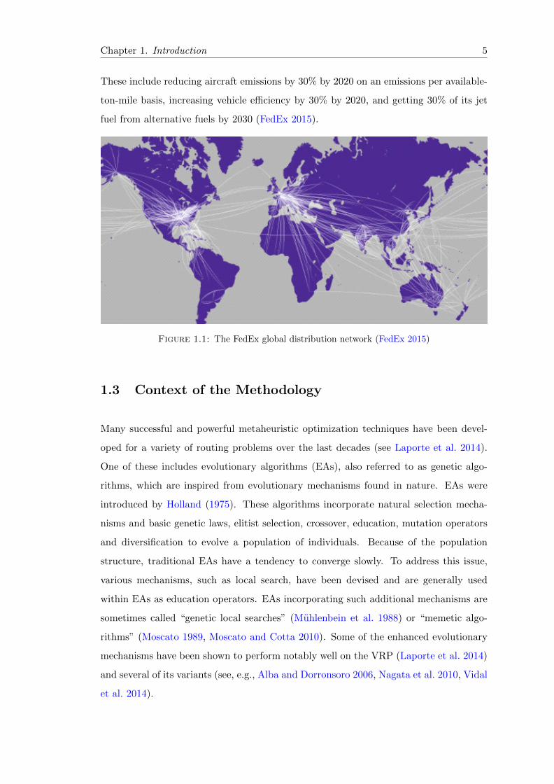
We now provide a practical example to show the relevance of the problems studied
in this thesis. FedEx is one of the world’s largest express transportation companies,
providing fast and reliable deliveries to more than 220 countries and territories in 2015
(see Figure 1.1). The company uses a global air-and-ground network to speed up the
delivery of time-sensitive shipments, usually within two business days with a guaranteed
delivery time. More than 160,000 employees work for the company worldwide. The
average daily volume is approximately four million packages and 11 million pounds of
freight. The company serves more than 375 airports with 650 heterogeneous aircraft, the
delivery fleet includes more than 48,000 heterogeneous vehicles, the company owns 1,250
operating facilities and 12 air express hubs. In the context of green issues, FedEx has
made significant gains in meeting its sustainability objectives. In 2012, the company
achieved a 22% fuel efficiency improvement in the vehicle fleet since 2005, by using
hybrid trucks, for example. FedEx has set several goals to reduce its carbon footprint.
Chapter 1. Introduction 5
These include reducing aircraft emissions by 30% by 2020 on an emissions per available-
ton-mile basis, increasing vehicle efficiency by 30% by 2020, and getting 30% of its jet
fuel from alternative fuels by 2030 (FedEx 2015).
Figure 1.1: The FedEx global distribution network (FedEx 2015)
1.3 Context of the Methodology
Many successful and powerful metaheuristic optimization techniques have been devel-
oped for a variety of routing problems over the last decades (see Laporte et al. 2014).
One of these includes evolutionary algorithms (EAs), also referred to as genetic algo-
rithms, which are inspired from evolutionary mechanisms found in nature. EAs were
introduced by Holland (1975). These algorithms incorporate natural selection mecha-
nisms and basic genetic laws, elitist selection, crossover, education, mutation operators
and diversification to evolve a population of individuals. Because of the population
structure, traditional EAs have a tendency to converge slowly. To address this issue,
various mechanisms, such as local search, have been devised and are generally used
within EAs as education operators. EAs incorporating such additional mechanisms are
sometimes called “genetic local searches” (Muhlenbein et al. 1988) or “memetic algo-
rithms” (Moscato 1989, Moscato and Cotta 2010). Some of the enhanced evolutionary
mechanisms have been shown to perform notably well on the VRP (Laporte et al. 2014)
and several of its variants (see, e.g., Alba and Dorronsoro 2006, Nagata et al. 2010, Vidal
et al. 2014).

Chapter 1. Introduction 6
Other successful optimization techniques proposed for routing problems are variations of
local search algorithms, one of which is the large neighborhood search (LNS) algorithm
introduced by Shaw (1998). LNS iteratively improves a solution by using both destroy
and repair operators. Ropke and Pisinger (2006a) developed an extended LNS heuristic
for a variant of the VRP, called adaptive large neighborhood search (ALNS), in which the
LNS operators are combined within the algorithm and used with a frequency determined
by their performance during the algorithm. The authors showed that such combined
use of different local search operators yields a highly efficient method for the VRP. In a
latter study, Ropke and Pisinger (2006b) developed an improved version of the ALNS
algorithm. Finally, Pisinger and Ropke (2007) presented an unified ALNS framework to
solve five different variants of the VRP. The authors indicate that this framework can
be applied to many variants of routing problems.
This brief review shows that EAs and ALNS are the state-of-the-art methods for the VRP
and its variants. With this motivation, our methodology is based on the combination of
these two successful search paradigms.
1.4 General Research Contributions
The general research contributions of this thesis are threefold:
1. To analyze and investigate heterogeneous routing problems, to introduce new vari-
ants involving location aspects and environmental externalities, in particular pol-
lution arising from fuel consumption.
2. To develop powerful metaheuristics capable of solving a wide variety of problems
with appropriate enhancements.
3. To derive several managerial insights into the interaction of location, fleet com-
position and routing decisions on key performance indicators, both for long-haul
transportation and city logistics.
The interactions between the three main themes of the thesis are depicted in Figure 1.2.

Chapter 1. Introduction 7
Heterogeneous
vehicle routing Facility
location
Vehicle emissions and
fuel consumption
Chapters 2 and 3Chapter 4
Chapter 6
Chapter 5
Figure 1.2: A schematic representation of the thesis structure
1.5 Specific Objectives
The remainder of this thesis is made up of five main chapters, followed by conclusions.
Here are the specific research objectives of Chapter 2 “Thirty Years of Heterogeneous
Vehicle Routing”:
• to classify heterogeneous vehicle routing problems,
• to present a comprehensive and up-to-date review of the existing studies by in-
cluding industrial applications and case studies,
• to comparatively analyze the performance of the state-of-the-art metaheuristic
algorithms.

Chapter 1. Introduction 8
Here are the specific research objectives of the Chapter 3 “A Hybrid Evolutionary Al-
gorithm for Heterogeneous Fleet Vehicle Routing Problems with Time Windows”:
• to review the latest developments on vehicle routing problems, and identify the
state-of-the-art in solution techniques,
• to introduce several algorithmic improvements to existing techniques,
• to devise a Hybrid Evolutionary Algorithm (HEA) capable of solving the het-
erogeneous fleet vehicle routing problems with time windows in which various
algorithmic components can be combined,
• to perform extensive computational experiments on benchmark instances.
Here are the specific research objectives of the Chapter 4 “The Fleet Size and Mix
Location-Routing Problem with Time Windows: Formulations and a Heuristic Algo-
rithm”:
• to identify the latest developments on location-routing problems,
• to formulate the Fleet Size and Mix Location-Routing Problem with Time Win-
dows (FSMLRPTW),
• to adapt the HEA for solving the FSMLRPTW,
• to perform extensive computational experiments.
Here are the specific research objectives of the Chapter 5 “The Fleet Size and Mix
Pollution-Routing Problem”:
• to identify functions for modelling fuel and CO2 emissions for heterogeneous vehicle
routing,
• to formulate the Fleet Size and Mix Pollution-Routing Problem (FSMPRP),
• to adapt the HEA for solving the FSMPRP,
• to perform analyses leading to managerial insights.

Chapter 1. Introduction 9
Here are the specific research objectives of the Chapter 6 “The impact of location, fleet
composition and routing on emissions in urban freight distribution”:
• to investigate the combined impact of depot location, fleet composition and routing
decisions on vehicle emissions in urban freight distribution characterized by several
speed limits,
• to devise a heuristic algorithm to solve the problem,
• to perform analyses in order to provide several insights.

Chapter 2
Thirty Years of Heterogeneous
Vehicle Routing
10

Chapter 2. Thirty Years of Heterogeneous Vehicle Routing 11
Abstract
It has been around thirty years since the heterogeneous vehicle routing problem was in-
troduced, and significant progress has since been made on this problem and its variants.
The aim of this survey paper is to classify and review the literature on heterogeneous
vehicle routing problems. The paper also presents a comparative analysis of the meta-
heuristic algorithms that have been proposed for these problems.
Keywords. vehicle routing; heterogeneous fleet; fleet size and mix; review
2.1 Introduction
In the classical Vehicle Routing Problem (VRP) introduced by Dantzig and Ramser
(1959), the aim is to determine an optimal routing plan for a fleet of homogeneous
vehicles to serve a set of customers, such that each vehicle route starts and ends at
the depot, each customer is visited once by one vehicle, and some side constraints are
satisfied. There exists a rich literature on the VRP and its variants, see, e.g., the surveys
by Cordeau et al. (2007) and Laporte (2009), and the books by Golden et al. (2008) and
Toth and Vigo (2014).
In most practical distribution problems, customer demands are served by means of a
heterogeneous fleet of vehicles (see, e.g., Hoff et al. 2010, FedEx 2015, TNT 2015).
Fleet dimensioning or composition is a common problem in industry and the trade-off
between owning and keeping a fleet and subcontracting transportation is a challenging
decision for companies. Fleet dimensioning decisions predominantly involve choosing the
number and types of vehicles to be used, where the latter choice is often characterized
by vehicle capacities. These decisions are affected by several market variables such as
transportation rates, transportation costs and expected demand.
The extension of the VRP in which one must additionally decide on the fleet composition
is known as the Heterogeneous Vehicle Routing Problem (HVRP). HVRPs are rooted
in the seminal paper of Golden et al. (1984) published some thirty years ago and have
recently evolved into a rich research area. There have also been several classifications
of the associated literature from different perspectives. Baldacci et al. (2008) provided
a general overview of papers with a particular focus on lower bounding techniques and

Chapter 2. Thirty Years of Heterogeneous Vehicle Routing 12
heuristics. The authors also compared the performance of existing heuristics described
until 2008 on benchmark instances. Baldacci et al. (2010a) presented a review of exact
algorithms and a comparison of their computational performance on the capacitated
VRP and HVRPs, while Hoff et al. (2010) reviewed several industrial aspects of combined
fleet composition and routing in maritime and road-based transportation. More recently,
Irnich et al. (2014) briefly reviewed papers on HVRPs published from 2008 to 2014.
This paper makes three main contributions. The first is to classify heterogeneous vehicle
routing problems. The second is to present a comprehensive and up-to-date review of
the existing studies. The third is to comparatively analyze the performance of the
state-of-the-art metaheuristic algorithms. Our review differs from the previous ones by
including references that have appeared since 2008, by comparing heuristic algorithms,
and by including industrial applications and case studies.
The remainder of this paper is structured as follows. The HVRPs and its variants
are described and classified in Section 2.2. Extended reviews of the three main problem
types, namely the Fleet Size and Mix Vehicle Routing Problem, the Heterogeneous Fixed
Fleet Vehicle Routing Problem and the Fleet Size and Mix Vehicle Routing Problem with
Time Windows are presented in Sections 2.3, 2.4 and 2.5, respectively. Reviews of the
other variants, extensions and case studies are presented in Sections 2.6 and 2.7. A
tabulated summary of the literature and comparisons of the state-of-the-art heuristic
algorithms are provided in Section 2.8. The paper closes with some concluding remarks
and future research directions in Section 2.9.
2.2 Classification of the Heterogeneous Vehicle Routing
Problem
We first define and classify the variants of HVRPs in Section 2.2.1, and then present
three mathematical formulations in Section 2.2.2.
2.2.1 Problem definition and classification
HVRPs generally consider a limited or an unlimited fleet of capacitated vehicles, where
each vehicle has a fixed cost, in order to serve a set of customers with known demands.

Chapter 2. Thirty Years of Heterogeneous Vehicle Routing 13
These problems consist of determining the fleet composition and vehicle routes, such
that the classical VRP constraints are satisfied. Two major HVRPs are the Fleet Size
and Mix Vehicle Routing Problem (FSM1) introduced by Golden et al. (1984) which
works with an unlimited heterogeneous fleet, and the Heterogeneous Fixed Fleet Vehicle
Routing Problem (HF) introduced by Taillard (1999) in which the fleet is predetermined.
Other variants of the FSM and the HF also exist. In what follows, we will classify the
main variants with respect to two criteria: (i) objectives and (ii) presence or absence of
time window constraints. We will also mention other HVRP variants and extensions.
2.2.1.1 Objectives
The objective of both the FSM and the HF is to minimize a total cost function which in-
cludes fixed (F) and variable (V) vehicle costs. We now differentiate between five impor-
tant variants: 1) the FSM with fixed and variable vehicle costs, denoted by FSM(F,V),
introduced by Ferland and Michelon (1988); 2) the FSM with fixed vehicle costs only,
denoted FSM(F), introduced by Golden et al. (1984); 3) the FSM with variable vehicle
costs only, denoted by FSM(V), introduced by Taillard (1999); 4) the HF with fixed and
variable vehicle costs, denoted by HF(F,V), introduced by Li et al. (2007); 5) the HF
with variable vehicle costs only, denoted by HF(V), introduced by Taillard (1999).
2.2.1.2 Time windows
Two natural extensions of the FSM and HF arise when time window constraints are
imposed on the start of service at each customer location. These problems are denoted
by FSMTW and HFTW, respectively. In these extensions, two measures are used to
compute the total cost to be minimized: 1) The first is based on the en-route time
(T) which is the sum of the fixed vehicle cost and the trip duration but excludes the
service time. In this case, service times are used only to check route feasibility and for
performing adjustments to the departure time from the depot in order to minimize pre-
service waiting times; 2) The second cost measure is based on distance (D) and consists
1Traditionally, the Fleet Size and Mix Vehicle Routing Problem has been abbreviated as FSMVRP,and its counterpart with time windows as FSMVRPTW. A similar convention has been adopted for theHeterogeneous Fixed Fleet Vehicle Routing Problem, by using HFFVRP and HFFVRPTW to denoteits versions without and with time windows, respectively. In our view, some of these abbreviations areexcessively long and defy the purpose of using shorthand notation. Hence we introduce shorter andsimpler abbreviations in this paper.

Chapter 2. Thirty Years of Heterogeneous Vehicle Routing 14
of the fixed vehicle cost and the distance traveled by the vehicle, as is the case in the
standard VRP with Time Windows (VRPTW) (Solomon 1987).
The FSM and HF, combined with the two objectives above, give rise to four problem
types: 1) the FSMTW with objective T, denoted by FSMTW(T), introduced by Liu and
Shen (1999b); 2) the FSMTW with objective D, denoted by FSMTW(D), introduced by
Braysy et al. (2008); 3) the HFTW with objective T, denoted by HFTW(T), introduced
by Paraskevopoulos et al. (2008); 4) the HFTW with objective D, denoted by HFTW(D),
recently introduced by Koc et al. (2015).
2.2.1.3 Other variants
More involved variants of the FSM or of the HF have been defined, including those
with multiple depots (see Dondo and Cerda 2007, Bettinelli et al. 2011, 2014). Other
extensions include stochastic demand (Teodorovic et al. 1995), pickups and deliveries
(Irnich 2000, Qu and Bard 2014), multi-trips (Prins 2002, Seixas and Mendes 2013),
the use of external carriers (Chu 2005, Potvin and Naud 2011), backhauls (Belmecheri
et al. 2013, Salhi et al. 2013), open routes (Li et al. 2012), overloads (Kritikos and
Ioannou 2013), site-dependencies (Nag et al. 1988, Chao et al. 1999), multi-vehicle task
assignment (Franceschelli et al. 2013), green routing (Juan et al. 2014, Koc et al. 2014),
single and double container loads (Lai et al. 2013), two-dimensional loading (Leung et
al. 2013, Dominguez et al. 2014), time-dependencies (Afshar-Nadjafi and Afshar-Nadjafi
2014), multi-compartments (Wang et al. 2014), multiple stacks (Iori and Riera-Ledesma
2015) and collection depot (Yao et al. 2015).
2.2.2 Mathematical formulations
We now present three formulations for the HVRP, two based on commodity flows and
one based on set partitioning. The common notations of all three formulations are as
follows. Each customer i has a non-negative demand qi. Let H = 1, . . . , k be the set
of available vehicle types. Let th and Qh denote the fixed vehicle cost and the capacity
of vehicle of type h ∈ H, respectively. Let mh be the available number of vehicles of
type h.

Chapter 2. Thirty Years of Heterogeneous Vehicle Routing 15
2.2.2.1 Single-commodity flow formulation
The HVRP is modeled on a complete graph G = (N ,A), where N = 0, . . . , n is the
set of nodes, node 0 corresponds to the depot, and A = (i, j) : 0 ≤ i, j ≤ n, i 6= j
denote the set of arcs. The customer set is Nc = N\0. Let chij be the travel cost on
arc (i, j) ∈ A by a vehicle of type h. Furthermore, let fhij be the amount of commodity
transported on arc (i, j) ∈ A by a vehicle of type h and let the binary variable xhij be
equal to 1 if and only if a vehicle of type h ∈ H travels on arc (i, j) ∈ A.
The single-commodity flow formulation of Baldacci et al. (2008) for the HVRP is as
follows:
Minimize∑h∈H
∑j∈Nc
thxh0j +∑h∈H
∑(i,j)∈A
chijxhij (2.1)
subject to∑j∈Nc
xh0j ≤ mh h ∈ H (2.2)
∑h∈H
∑j∈N
xhij = 1 i ∈ Nc (2.3)
∑h∈H
∑i∈N
xhij = 1 j ∈ Nc (2.4)∑h∈H
∑j∈N
fhji −∑h∈H
∑j∈N
fhij = qi i ∈ Nc (2.5)
qjxhij ≤ fhij ≤ (Qh − qi)xhij (i, j) ∈ A, h ∈ H (2.6)
xhij ∈ 0, 1 (i, j) ∈ A, h ∈ H (2.7)
fhij ≥ 0 (i, j) ∈ A, h ∈ H. (2.8)
In this formulation, the objective function (2.1) minimizes the sum of vehicle fixed costs
and the total travel cost. The maximum number of available vehicles of each type is
imposed by constraints (2.2). In the case of the FSM, an unlimited number of vehicles for
each vehicle type h (mh = |Nc|) are available, which effectively renders constraints (2.2)
redundant. Constraints (2.3) and (2.4) ensure that each customer is visited exactly once.
Constraints (2.5) and (2.6) define the commodity flows. Finally, constraints (2.7) and
(2.8) enforce the integrality and non-negativity restrictions on the variables.
Chapter 2. Thirty Years of Heterogeneous Vehicle Routing 16
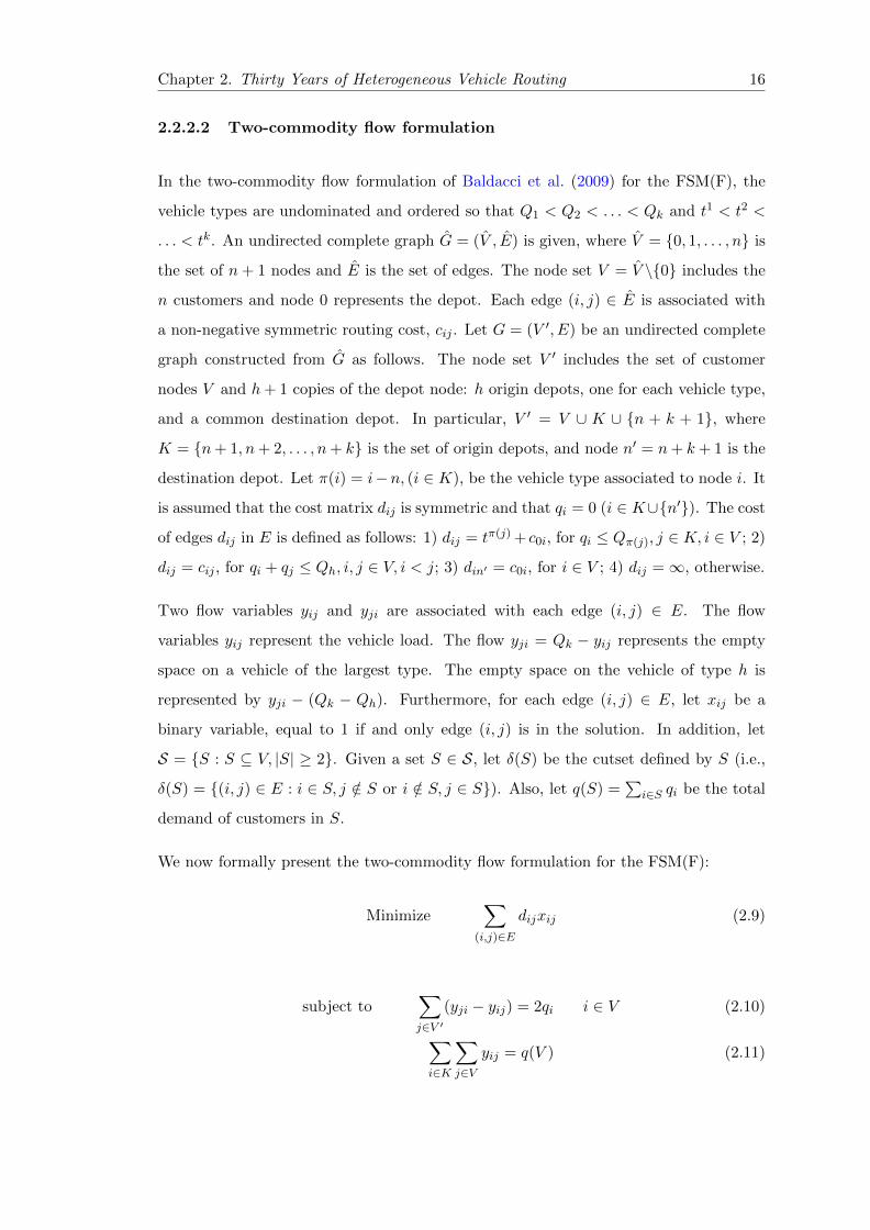
2.2.2.2 Two-commodity flow formulation
In the two-commodity flow formulation of Baldacci et al. (2009) for the FSM(F), the
vehicle types are undominated and ordered so that Q1 < Q2 < . . . < Qk and t1 < t2 <
. . . < tk. An undirected complete graph G = (V , E) is given, where V = 0, 1, . . . , n is
the set of n+ 1 nodes and E is the set of edges. The node set V = V \0 includes the
n customers and node 0 represents the depot. Each edge (i, j) ∈ E is associated with
a non-negative symmetric routing cost, cij . Let G = (V ′, E) be an undirected complete
graph constructed from G as follows. The node set V ′ includes the set of customer
nodes V and h+ 1 copies of the depot node: h origin depots, one for each vehicle type,
and a common destination depot. In particular, V ′ = V ∪ K ∪ n + k + 1, where
K = n+ 1, n+ 2, . . . , n+ k is the set of origin depots, and node n′ = n+ k + 1 is the
destination depot. Let π(i) = i−n, (i ∈ K), be the vehicle type associated to node i. It
is assumed that the cost matrix dij is symmetric and that qi = 0 (i ∈ K∪n′). The cost
of edges dij in E is defined as follows: 1) dij = tπ(j) + c0i, for qi ≤ Qπ(j), j ∈ K, i ∈ V ; 2)
dij = cij , for qi + qj ≤ Qh, i, j ∈ V, i < j; 3) din′ = c0i, for i ∈ V ; 4) dij =∞, otherwise.
Two flow variables yij and yji are associated with each edge (i, j) ∈ E. The flow
variables yij represent the vehicle load. The flow yji = Qk − yij represents the empty
space on a vehicle of the largest type. The empty space on the vehicle of type h is
represented by yji − (Qk − Qh). Furthermore, for each edge (i, j) ∈ E, let xij be a
binary variable, equal to 1 if and only edge (i, j) is in the solution. In addition, let
S = S : S ⊆ V, |S| ≥ 2. Given a set S ∈ S, let δ(S) be the cutset defined by S (i.e.,
δ(S) = (i, j) ∈ E : i ∈ S, j /∈ S or i /∈ S, j ∈ S). Also, let q(S) =∑
i∈S qi be the total
demand of customers in S.
We now formally present the two-commodity flow formulation for the FSM(F):
Minimize∑
(i,j)∈E
dijxij (2.9)
subject to∑j∈V ′
(yji − yij) = 2qi i ∈ V (2.10)
∑i∈K
∑j∈V
yij = q(V ) (2.11)

Chapter 2. Thirty Years of Heterogeneous Vehicle Routing 17
∑j∈V
yjn′ = 0 (2.12)
∑i,j∈δ(b)
xij = 2 ∀b ∈ V (2.13)
∑i∈K
∑j∈V
xij =∑j∈V
xjn′ (2.14)
yij + yji = Qkxij (i, j) ∈ E (2.15)∑i,j∈δ(S)
xij ≥∑i∈K
∑j∈V
xij K ⊂ S, S ⊆ K ∪ V (2.16)
yij ≤ Qπ(i) i ∈ K, j ∈ V (2.17)
yij ≥ 0, yji ≥ 0 (i, j) ∈ E (2.18)
xij ∈ 0, 1 (i, j) ∈ E. (2.19)
Constraints (2.10)–(2.12) and (2.18) define a feasible flow pattern. Constraints (2.12)
guarantee that the inflow at node n′ is equal to 0. Constraints (2.13) ensure that any
feasible solution must contain two edges incident to each customer. Constraints (2.14)
impose that if p =∑
i∈K∑
j∈V xij vehicles leave node set K, then exactly p vehicles
must enter node n′. Constraints (2.15) define the relation among variables in a feasible
solution. Constraints (2.16) forbid the presence of simple paths starting and ending
at nodes in K. The capacity requirements for each vehicle are imposed by constraints
(2.17). Finally, constraints (2.18) and (2.19) enforce the integrality and non-negativity
restrictions on the variables.
2.2.2.3 Set partitioning formulation
The set partitioning formulation of Baldacci and Mingozzi (2009) works with an undi-
rected graph G = (V ′, E), where V ′ = 0, . . . , n is the set of n+ 1 nodes and E is the
set of edges. Node 0 represents the depot and node set V = V ′\0 corresponds to n
customers. A route R = (0, i1, . . . , ir, 0) performed by a vehicle of type h, is a simple
cycle in G passing through the depot and customers i1, . . . , ir ⊆ V , with r ≥ 1. Let
<h be the index set of all feasible routes of vehicle type h ∈ H and let < =⋃h∈H<h.
For each route ` ∈ <h is associated a routing cost ch` . Let <hi ⊂ <h be the index subset
of the routes of a vehicle of type h covering customer i ∈ V . Let Rh` be the subset of
customers visited by route ` ∈ <h. Furthermore, let yh` be a binary variable that is equal
to 1 if and only if route ` ∈ <h is chosen in the solution.
Chapter 2. Thirty Years of Heterogeneous Vehicle Routing 18
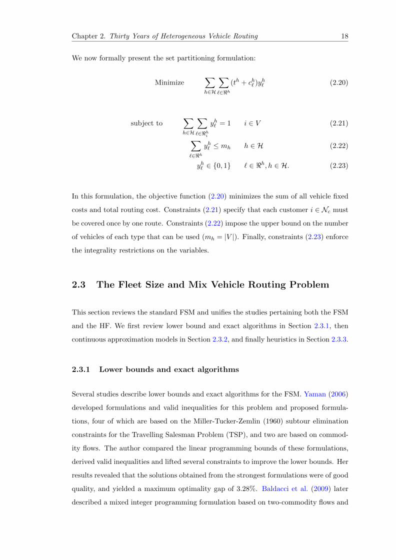
We now formally present the set partitioning formulation:
Minimize∑h∈H
∑`∈<h
(th + ch` )yh` (2.20)
subject to∑h∈H
∑`∈<h
i
yh` = 1 i ∈ V (2.21)
∑`∈<h
yh` ≤ mh h ∈ H (2.22)
yh` ∈ 0, 1 ` ∈ <h, h ∈ H. (2.23)
In this formulation, the objective function (2.20) minimizes the sum of all vehicle fixed
costs and total routing cost. Constraints (2.21) specify that each customer i ∈ Nc must
be covered once by one route. Constraints (2.22) impose the upper bound on the number
of vehicles of each type that can be used (mh = |V |). Finally, constraints (2.23) enforce
the integrality restrictions on the variables.
2.3 The Fleet Size and Mix Vehicle Routing Problem
This section reviews the standard FSM and unifies the studies pertaining both the FSM
and the HF. We first review lower bound and exact algorithms in Section 2.3.1, then
continuous approximation models in Section 2.3.2, and finally heuristics in Section 2.3.3.
2.3.1 Lower bounds and exact algorithms
Several studies describe lower bounds and exact algorithms for the FSM. Yaman (2006)
developed formulations and valid inequalities for this problem and proposed formula-
tions, four of which are based on the Miller-Tucker-Zemlin (1960) subtour elimination
constraints for the Travelling Salesman Problem (TSP), and two are based on commod-
ity flows. The author compared the linear programming bounds of these formulations,
derived valid inequalities and lifted several constraints to improve the lower bounds. Her
results revealed that the solutions obtained from the strongest formulations were of good
quality, and yielded a maximum optimality gap of 3.28%. Baldacci et al. (2009) later
described a mixed integer programming formulation based on two-commodity flows and
Chapter 2. Thirty Years of Heterogeneous Vehicle Routing 19
developed two new classes of valid inequalities for the FSM. These inequalities, which
were new covering-type and fleet-dependent capacity inequalities, aimed to increase the
lower bounds. The authors showed that their model was quite compact when compared
with previous formulations, and that its linear relaxation had a reasonable quality. Fleet-
dependent capacity inequalities were able to improve the lower bound by about 5% on
average, and the new covering inequalities improved it by about 2.5%. Pessoa et al.
(2009) presented a robust branch-cut-and-price algorithm for the FSM. Q-routes were
associated with the columns, which are relaxations of capacitated elementary routes that
make the pricing problem solvable in pseudo-polynomial time. These authors also pro-
posed new families of cuts which were expressed on a large set of variables and did not
increase the complexity of the pricing subproblem. The results showed that instances
up to 75 nodes can be solved to optimality, a significant improvement with respect to
previous exact algorithms.
Three unified exact algorithms are available to solve both the FSM and the HF. Choi
and Tcha (2007) developed a column generation algorithm and solved its linear pro-
gramming relaxation by column generation. They modified several dynamic program-
ming algorithms for the classical VRP to efficiently generate feasible columns and then
applied a branch-and-bound procedure to obtain an integer solution. Their results con-
firmed the superiority of this method over existing algorithms, both in terms of solution
quality and computation time. Baldacci and Mingozzi (2009) later introduced a unified
exact algorithm based on the set partitioning formulation. Three types of bounding
procedures were used, based on the LP-relaxation and on Lagrangean relaxation. The
new lower bounds were tighter than all previously known lower bounds. The last exact
algorithm for the FSM and the HF was, to our knowledge, presented by Baldacci et al.
(2010b). It combines several dual ascent procedures to generate a near-optimal dual so-
lution of the set partitioning model and it adds valid inequalities to the set partitioning
formulation within a column-and-cut generation algorithm to close the integrality gap
left by the dual ascent procedures. The final dual solution is then defined to generate a
reduced problem containing all optimal integer solutions. This algorithm outperformed
all other available exact algorithms.

Chapter 2. Thirty Years of Heterogeneous Vehicle Routing 20
2.3.2 Continuous approximation models
Jabali et al. (2012a) developed a continuous approximation model for the FSM. Their
model builds upon the work of Daganzo (1984a,b) and of Newell et al. (1986), where
the latter introduced a continuous approximation model for the VRP. This model can
be used at an aggregate level to analyze capacity scenarios and various cost scenarios.
The authors incorporated mixed fleet considerations to the model of Newell et al. (1986)
in which the vehicle routes are based on a partition of a ring-radial region into zones,
each of which is serviced by a single vehicle. They presented a mixed integer non-linear
formulation and developed several upper and lower bounding procedures for it. The
performance of the model was tested on several instances. Computational results showed
that the two proposed upper bounding procedures were more reliable than solving the
original model by an off-the-shelf software. They also demonstrated the sensitivity of
the models with respect to several parameters such as the vehicle variable and fixed
costs, the route duration limit and customer density.
2.3.3 Heuristics
This section presents a review of heuristic methods for the FSM. We first review popu-
lation search heuristics in Section 2.3.3.1, then tabu search heuristics in Section 2.3.3.2,
and finally other heuristics in Section 2.3.3.3.
2.3.3.1 Population search heuristics
In contrast to the VRP, only a few population search heuristics have been developed for
the FSM. Ochi et al. (1998a) described a hybrid metaheuristic which integrates genetic
algorithms and scatter search with a decomposition-into-petals procedure. Ochi et al.
(1998b) later used the same idea within parallel genetic algorithms. Several results of
Taillard (1999) were improved with this method. However, Ochi et al. (1998a,b) did
not report the exact solution values. Lima et al. (2004) proposed a memetic algorithm
which is a hybrid of a genetic algorithm and of the simulated annealing heuristic of
Osman (1993), and was able to find eight new best-known solutions for the Golden et
al. (1984) instances. Another genetic algorithm was developed by Liu et al. (2009) who
used several heuristics to generate the initial solution. Out of the 20 instances of Golden

Chapter 2. Thirty Years of Heterogeneous Vehicle Routing 21
et al. (1984), 14 solutions were matched and one was improved when compared with
existing algorithms such as those of Brandao et al. (2009) and Choi and Tcha (2007).
Several population heuristics for the FSM and the HF are based on variants of the split
procedure of Prins (2004). Prins (2009) developed two memetic algorithms hybridized
with a local search, based on chromosomes encoded as giant tours and without trip
delimiters. The methods optimally splits giant tours into feasible routes and assigns a
suitable vehicle type to them. The method creates new solutions from a single solution at
each iteration by performing mutations and local search operations. The results revealed
that the proposed method was able to efficiently handle the problems. The authors also
generated a set of HF instances based on real distances from French counties and ranging
from 50 to more than 250 customers. In a recent study, Vidal et al. (2014) introduced
a genetic algorithm using a unified component based solution framework for different
variants of the VRPs, including the FSM, the FSMTW(T) and the FSMTW(D). The
authors used problem-independent local search operators such as crossover, split and
a number of diversification mechanisms. A unified route-evaluation methodology was
developed to increase the effectiveness of the local search. This methodology is primarily
based on two procedures: move evaluations as a concatenation of known subsequences
and information preprocessing on subsequences, as well as other well-known procedures.
Excellent results were obtained on the FSM, the FSMTW(T) and the FSMTW(D),
which will be presented in more detail in Section 2.8.2.3.
2.3.3.2 Tabu search heuristics
The first tabu search heuristic for the FSM is probably that of Osman and Salhi (1996)
who modified the route perturbation procedure of Salhi and Rand (1993). The ex-
isting results for the benchmark instances were improved with the proposed method.
Gendreau et al. (1999) later developed a tabu search heuristic which embedded the gen-
eralized insertion heuristic of Gendreau et al. (1992) and the adaptive memory procedure
of Rochat and Taillard (1995). Their results were compared with those of Taillard (1999)
and confirmed the superiority of their algorithm. Wassan and Osman (2002) presented
a reactive tabu search heuristic in which several neighborhoods and special data struc-
tures were integrated and contained an intensification phase to trigger switches between
simple moves. Several deterministic moves were introduced to diversify the search. The

Chapter 2. Thirty Years of Heterogeneous Vehicle Routing 22
authors also proposed special data structures to explore various neighbourhoods. The
method was capable of generating a number of best-known solutions. Another tabu
search heuristic was developed by Lee et al. (2008) which applied a modified sweeping
method with set partitioning on a giant tour was used to create initial solutions. An
optimal vehicle assigment was performed for the set of routes, whenever the algorithm
identified a new solution. Competitive results were obtained on the Golden et al. (1984)
instances and several new best-known solutions were found. Finally, Brandao et al.
(2009) proposed a tabu search algorithm in which three procedures are used to generate
the initial solutions, and three moves are defined for the neighborhoods: single insertion,
double insertion and swap. The algorithm also used intensification and diversification
procedures during the search. The proposed method was able to obtain high quality
solutions, including five new best-known solutions.
2.3.3.3 Other heuristics
Several versions of constructive heuristics and many other heuristics have been pro-
posed for the FSM over the last thirty years. Golden et al. (1984) formally described
and formulated the FSM. They also developed some heuristics based on the Clarke and
Wright (1964) savings algorithm and on the partitioning of a giant tour into routes
suitable for various vehicle types, using the Or-opt (1976) improvement mechanism for
the TSP. They also described a procedure to calculate a lower bound. They applied
the Fisher and Jaikumar (1981) heuristic to solve the generalized assignment problem
for the assignment of customers to vehicles. Gheysens et al. (1984) used the Golden
et al. (1984) lower bounding procedure to create a new heuristic. Their method first
generated a fleet mix and then solved the resulting problem as a VRP. In a later study,
Gheysens et al. (1986) showed that the proposed lower bound based heuristic of Ghey-
sens et al. (1984), performed in general better than the heuristics of Golden et al. (1984).
However, computation times were much larger and finding a feasible solution was not
guaranteed. Desrochers and Verhoog (1991) developed an improved savings heuristic
which is a matching based savings algorithm using successive route merging procedures.
The method selects the best solution by solving a weighted matching problem at each
iteration. Competitive results were obtained with respect to previous studies. Salhi
et al. (1992) presented a mathematical formulation and described a perturbation based

Chapter 2. Thirty Years of Heterogeneous Vehicle Routing 23
heuristic which was tested on 20 benchmark instances and yielded several best-known so-
lutions. Salhi and Rand (1993) described a more advanced constructive heuristic which
starts from a solution obtained by solving a VRP with a single vehicle capacity, selected
among the available ones. Several procedures are then iteratively applied to improve
it which is achieved by changing the vehicle type assigned to each route, merging or
removing routes and moving customers from one route to another. On average, the pro-
posed method performed better than the earlier algorithms. Renaud and Boctor (2002)
proposed a sweep-based heuristic which extended the work of Renaud et al. (1996). The
algorithm first creates a large number of routes that can be served by one or two vehicles
and a set partitioning problem is then solved optimally, in polynomial time, to select
the routes and vehicles to use. The method outperformed the existing algorithms and
yielded competitive results with respect to tabu search. Han and Cho (2002) presented
another constructive heuristic algorithm which uses generic intensification and diversi-
fication procedures. The method incorporates several mechanisms from deterministic
variants of simulated annealing like threshold accepting and the great deluge algorithm
(Dueck 1993). The method performed well on the Golden et al. (1984) small-size in-
stances, but was dominated by the heuristics of Taillard (1999) and Gendreau et al.
(1999) on the large-size instances.
The FSM and the HF are simultaneously considered in several papers. The earliest such
work is by Taillard (1999) who developed a heuristic column generation algorithm. His
method solved a homogeneous VRP by means of the Rochat and Taillard (1995) adaptive
memory procedure for each of the vehicle type, where it was assumed that the number
of available vehicles is unlimited. This heuristic outperformed that of Osman and Salhi
(1996) on the eight largest FSM instances. The method was also tested for the HF on
new benchmark instances. Imran et al. (2009) later adapted a variable neighborhood
search algorithm for the FSM and the HF. Several additional features were added to
the method: an adaptation of local search procedures including Dijkstra’s algorithm, a
diversification procedure, and the use of a dummy empty route during the search. This
heuristic yielded competitive results on benchmark instances and was able to find several
new best-knowns solutions. A hybrid algorithm that considered both problems was later
proposed by Subramanian et al. (2012). It includes an iterated local search (ILS)-based
heuristic to generate columns in a set partitioning formulation. Competitive results and

Chapter 2. Thirty Years of Heterogeneous Vehicle Routing 24
new best-known solutions were obtained on benchmark instances which include large-
size instances involving up to 360 customers. The same authors presented improved
results by integrating the ILS with a variable neighborhood descent procedure and with
a random neighborhood ordering scheme in the local search phase (Penna et al. 2013).
The performance of the method was tested on 52 benchmark instances with up to 100
customers. Four new best-known solutions were obtained and 42 best-known results
were matched.
2.4 The Heterogeneous Fixed Fleet Vehicle Routing Prob-
lem
To our knowledge, no exact algorithm has specifically been designed for the standard HF.
However, several exact algorithms jointly consider the FSM and the HF. We therefore
focus exclusively on heuristics described for the HF. We first review tabu search heuristics
in Section 2.4.1, and then other heuristics in Section 2.4.2.
2.4.1 Tabu search heuristics
Euchi and Chabchoub (2010) designed a hybrid tabu search embedded within an adap-
tive memory heuristic for the HF. This algorithm generates three initial solutions, and
at each iteration the current solution is improved by several constructive methods. The
results obtained on benchmark instances were competitive in terms of solution quality
and computation time. Another tabu search algorithm was proposed by Brandao et al.
(2011). The algorithm is initiated with a giant tour over all customers which is then
partitioned into routes that are later improved using four types of moves. Four new
best-known solutions were obtained on benchmark instances.
2.4.2 Other heuristics
Tarantilis et al. (2003) proposed a list-based threshold accepting metaheuristic for the
HF which explores the solution space to identify promising regions. The method was
competitive on benchmark instances and could find several new best-known solutions. In
a later study, the same authors developed a backtracking adaptive threshold accepting

Chapter 2. Thirty Years of Heterogeneous Vehicle Routing 25
algorithm (Tarantilis et al. 2004), which generalizes that of Tarantilis and Kiranoudis
(2001). The main difference between this method and the standard threshold accepting
heuristic is that the value of the threshold does not always decrease but can also increase.
New best solutions and better results were obtained compared with Taillard (1999).
The heuristic of Gencer et al. (2006) is based on the principle of first clustering and
then routing and considers the possibility of leasing vehicles when the size of the fleet
is insufficient. On average, the algorithm provided lower quality solutions than that
Tarantilis et al. (2004) but found better solutions in terms of vehicle capacity utilization.
Li et al. (2007) adapted their previous record-to-record travel algorithm (Li et al. 2005) to
solve the HF. The algorithm is a deterministic variant of a simulated annealing heuristic
and produced new best-known solutions. Li et al. (2010) later developed a multistart
adaptive memory programming and path relinking heuristic. This algorithm constructs
multiple provisional solutions which are then improved through a modified tabu search at
each iteration. New best-known solutions were found on two benchmark instances, and
for the others the method found solutions of a quality comparable to that of previous
algorithms. Liu (2013) developed a hybrid population heuristic with embedded local
search mechanisms to diversify the population. Competitive results were obtained within
short computation times. Naji-Azimi and Salari (2013) solved the HF by developing a
mathematical formulation based heuristic algorithm. The method applies a mechanism
in which the initial solution is destroyed and repaired by solving a mathematical model
to optimality. Three new best-known solutions were obtained on bencmark instances.
2.5 The fleet size and mix vehicle routing problem with
time windows
We now review the existing literature on the FSMTW. This variant of the FSM has
received considerable attention, which is the reason why it is presented in a separate
section. To the best of our knowledge, apart from a simple branch-and-bound scheme
(Ferland and Michelon 1988), no exact algorithm has yet been proposed for the standard
FSMTW. We first review tabu search heuristics in Section 2.5.1, followed by other
heuristics in Section 2.5.2.

Chapter 2. Thirty Years of Heterogeneous Vehicle Routing 26
2.5.1 Tabu search heuristics
Paraskevopoulos et al. (2008) developed a two-phase heuristic based on a hybridized
tabu search algorithm for the FSMTW(T) and the HFTW(T). In the first phase, ini-
tial solutions are generated by a semi-parallel construction heuristic which is followed
by a sophisticated ejection chain procedure in the second phase. The quality of the
solutions is further improved using variable neighborhood tabu search. To diversify the
solutions, the authors describe a specialized shaking mechanism. Computational ex-
periments conducted on the FSMTW benchmark data sets allowed the identification
of better solutions than those reported by Dell’Amico et al. (2007), by about 3.4% on
average. New benchmark results for the HFTW(T) were also presented for the first
time.
2.5.2 Other heuristics
Ferland and Michelon (1988) showed that the VRPTW can be extended to the hetero-
geneous VRPTW. They presented three heuristic algorithms: discrete approximation,
assignment and matching, as well as two simple branch-and-bound procedures. Liu
and Shen (1999b) described a heuristic for the FSMTW(T) which starts by determin-
ing an initial solution through an adaptation of the Clarke and Wright (1964) savings
algorithm previously presented by Golden et al. (1984). The second stage improves
the initial solution by moving customers by means of parallel insertions. The algo-
rithm was tested on a set of 168 FSMTW benchmark instances derived from the set of
Solomon (1987) for the VRPTW and was also tested on the standard FSM. Dullaert
et al. (2002) described a sequential construction algorithm for the FSMTW(T). The
algorithm includes three insertion-based heuristics which are extensions of the I1 heuris-
tic of Solomon (1987) and of the Golden et al. (1984) vehicle insertion saving method.
Another paper on the FSMTW(T) is that of Dell’Amico et al. (2007) who developed
a multi-start parallel regret construction heuristic embedded within a ruin-and-recreate
metaheuristic. The proposed heuristic allows for the combination of routes into longer
routes requiring a larger vehicle, and the splitting of routes into smaller ones. It outper-
formed previously published heuristics. Repoussis and Tarantilis (2010) later developed
an adaptive memory programming algorithm for the FSMTW(T) which includes a prob-
abilistic construction heuristic, a diversification mechanism, a short-term memory tabu

Chapter 2. Thirty Years of Heterogeneous Vehicle Routing 27
search heuristic with edge-exchange neighbourhoods, speed-up procedures, and an it-
erated tabu search procedure working with a perturbation mechanism. Learning and
several frequency-based long term mechanisms are also embedded into the algorithm.
This method outperformed those presented in previous studies and improved upon 80
best-known solutions.
Braysy et al. (2008) presented a three-phase multi-restart deterministic annealing meta-
heuristic for the FSMTW(T) and the FSMTW(D). In this algorithm, solutions are
created by Clarke and Wright (1964) savings algorithm and by combining several diver-
sification strategies. The second stage aims to reduce the number of routes in the initial
solution by means of a greedy local search procedure. Four local search operators are
embedded within a deterministic annealing framework to guide the improvement process
in the final stage. The algorithm outperformed the earlier results on the FSMTW(T).
New benchmark results on the FSMTW(D) were also presented. In a later study, Braysy
et al. (2009) described a hybrid metaheuristic algorithm for large-scale FSMTW(D) in-
stances. They combined the well-known threshold acceptance heuristic with a guided
local search metaheuristic having several search limitation strategies. Computational
experiments yielded better results on the FSMTW(D) instances compared to those of
Braysy et al. (2008), and this algorithm was then used to solve a further 600 new
FSMTW(D) benchmark instances with up to 1000 customers.
Prieto et al. (2011) described an asynchronous situated coevolution algorithm for a het-
erogeneous vehicle routing problem with time windows which uses a situated coevolution
process inspired from the artificial life simulations. The authors showed that their open-
ended evolutionary simulation which includes an improvement procedure yields good
results. The performance was only tested on one instance with 20 nodes and 50 ships,
not part of the standard benchmark FSMTW(D) instances, and the solution consists of
a self-organized fleet of heterogeneous ships which satisfies the problem constraints and
the market requirements.
More recently, Chapter 3 presented a unified heuristic called a hybrid evolutionary algo-
rithm (HEA) for the FSMTW(T), the FSMTW(D), the HFTW(T) and the HFTW(D),
and were the ones who introduced the last variant. The HEA combines several meta-
heuristics principles such as heterogeneous adaptive large scale neighborhood search and
population search. The authors integrated within the HEA an innovative intensification

Chapter 2. Thirty Years of Heterogeneous Vehicle Routing 28
strategy on elite solutions, a new diversification scheme based on the regeneration and
the mutation procedures of solutions, and developed an advanced version of the split
algorithm of Prins (2009) to determine the best fleet mix for a set of routes. Exten-
sive computational experiments on benchmark instances showed that the HEA is highly
effective on all four problems.
2.6 Variants and Extensions
Both the FSM and the HF have given rise to a multitude of extensions which have
received particular attention in the last five years. In this section, we review such
variants and extensions, which are classified in Figure 2.1.
2.6.1 The multi-depot HVRP
The Multi-Depot FSM was introduced by Salhi and Sari (1997) who proposed a three-
level composite heuristic for it. An initial solution is first generated, a composite heuristic
is executed to improve the quality of the solution, and an extension of the composite
heuristic which considers all depots simultaneously is then applied. Several procedures of
the algorithm are taken from Salhi and Rand (1993). Salhi et al. (2014) later considered
the same problem by proposing a mixed integer linear programming formulation with
new valid inequalities and several variable settings. Furthermore, the authors developed
a variable neighborhood search heuristic equipped with a scheme for determining border-
line customers and combined with a local search method based on a multi-level heuristic.
The heuristic uses Dijkstra’s algorithm to optimally partition the routes. It includes a
diversification procedure and also contains a mechanism to aggregate the routes from
different depots and then to disaggregate them and assign them to different depots. In
total, 23 new best solutions out of the 26 benchmark instances were obtained, which
makes this heuristic highly competitive.
Several metaheuristics were developed for the Multi-Depot FSMTW. Thus Dondo and
Cerda (2007) proposed a mathematical model and a three-phase heuristic. The first
phase determines a set of cost effective clusters and the second phase assigns clusters to
vehicles and sequences them on each tour by using a cluster-based mathematical model.

Chapter 2. Thirty Years of Heterogeneous Vehicle Routing 29
Multiple depots
Pickup and delivery
Green
Backhauls
External carriers
Container loading
Split delivery
Open
HVRP variants
FSM: Salhi and Sari (1997), Salhi et al. (2014)
FSMTW: Dondo and Cerda (2007), Xu et al. (2012)
HFTW: Bettinelli et al. (2011)
Pickup and Delivery FSMTW: Irnich (2000)
Time Dependent HFTW: Afshar-Nadjafi and Afshar-Nadjafi (2014)
Multi Unmanned FSM: Levy et al. (2014)
HF: Kwon et al. (2013)
FSM: Kopfer and Kopfer (2013), Kopfer et al. (2014)
FSM with Multiple Driving Ranges: Juan et al. (2014)
FSMTW: Koç et al. (2014b)
HF: Tütüncü (2010)
HFTW: Belmecheri et al. (2013)
FSM: Salhi et al.(2013)
HF: Chu (2005), Bolduc et al. (2007), Bolduc et al. (2008), Potvin and Naud (2011)
FSMTW: Ceschia et al. (2011)
HF with Single and Double Contained Loads: Lai et al. (2013)
FSM with Two-Dimensional Loading: Leung et al. (2013), Dominguez et al. (2014)
HF: Tavakkoli et al. (2007)
FSMTW: Belfiore and Yoshizaki (2013)
HF with Configurable Vehicle Capacity: Qu and Bard (2013)
Pickup and Delivery FSMTW with Configurable Vehicle Capacity: Qu and Bard (2014)
HF: Li et al. (2012), Yousefikhoshbakht et al. (2014)
Others
Stochastic FSM: Teodorovi et al. (1995)
FSM with Fleet Dimensioning: Vis et al. (2005)
HF with a Synchronized Production and Distribution: Bolduc et al. (2006)
FSMTW with Independent Route Length: Tavakkoli et al. (2006)
HF with soft Time Windows: Yepes and Medina (2006)
FSMTW with Limited Transport Capacity: De la Cruz et al. (2013)
FSM with Multi-Vehicle Task Assignment: Franceschelli et al. (2013)
FSMTW with Overloads: Kritikos and Ioannou (2013)
Multi Trip FSMTW: Seixas and Mendes (2013)
HFTW with Hierarchical Objective: Jiang et al. (2014)
Multi-compartment HF: Wang et al. (2014)
Figure 2.1: A classification of HVRP variants

Chapter 2. Thirty Years of Heterogeneous Vehicle Routing 30
In the final phase, customer orders and scheduling of vehicle arrival times are opti-
mized by solving a mathematical model. Computational experiments were conducted
on adapted classical Solomon (1987) VRPTW instances with up to 100 nodes. In another
study, Xu et al. (2012) described a mathematical formulation and implemented a vari-
able neighborhood search algorithm. The authors designed a hybrid insert and exchange
operator for the shaking mechanism and implemented a best-improvement strategy to
increase solution quality and decrease the running time. No computational experiments
were conducted on the FSMTW since the authors only tested their algorithm on the
classical Golden et al. (1984) FSM instances.
Bettinelli et al. (2011) developed a branch-and-cut-and-price algorithm for the Multi-
Depot HFTW. They investigated several mixed strategies, such as initializing the re-
stricted master problem and repairing the columns in the restricted master problem by
removing cycles. Their results suggest that the number of different vehicle types, as op-
posed to the presence of multiple depots, makes the problem more difficult to solve. The
tightness of the time windows was also found to influence the difficulty of the problem.
Irnich (2000) introduced the Multi-Depot Pickup and Delivery FSMTW with a single
hub. In this problem, all routes have to visit the hub once, and are cycles that start from
and end at the same depot. The author developed a network model which computes
lower bounds and solves a set partitioning problem.
Afshar-Nadjafi and Afshar-Nadjafi (2014) studied a Time-Dependent Multi-Depot HFTW
and proposed a mathematical formulation along with a constructive heuristic with three
local search operators. Their results were compared on 180 test instances and indicate
that the proposed heuristic was able to identify solutions within 0.3% of optimality for
small size instances
Levy et al. (2014) introduced the Multi-Depot Multi-Unmanned FSM with Fuel Con-
straints where the different types of vehicles, between two and nine, are expected to refuel
at fuel stations or at depots as they run out of fuel. They used a variable neighbor-
hood descent (VND) and a variable neighborhood search (VNS). The authors presented
simulation results to test the efficiency of the method on a set of 23 instances on which
VND produced better solutions than VNS.

Chapter 2. Thirty Years of Heterogeneous Vehicle Routing 31
Dayarian et al. (2015) introduced the Multi-Depot FSMTW with deliveries to plants.
The problem is inspired by collection-redistribution activities in the raw-milk industry
of Quebec, where there is a need to satisfy the plant demands by delivering the supplies
collected earlier. The authors defined a new set covering model, a specialized cutting-
edge column generation procedure to solve its linear relaxation, and a new branching
strategy based on the special structure of the problem. Promising results were obtained
on instances with up to 50 producers.
2.6.2 The green HVRP
In recent years, green issues have received increased attention in the context of the VRP.
Thus, Kwon et al. (2013) studied a green extension of the HF in which the objective
is to minimize carbon emissions. The authors presented a mathematical formulation
and developed several tabu search algorithms. The authors performed a cost-benefit
assessment of the value of selling or purchasing of carbon emission rights. Their results
suggest that carbon emissions can be reduced without increasing costs due to the benefits
of carbon trading.
Juan et al. (2014) introduced the FSM with Multiple Driving Ranges in which the total
distance that each vehicle type can travel is limited. This problem arises in the routing
of electric and hybrid-electric vehicles which can only travel limited distances due to the
limited capacity of their batteries. The authors described a mathematical formulation
and developed a multi-round heuristic. The method is based on a biased randomized
algorithm which can be used alone to create alternative fleet choices whenever the fea-
sibility of the prespecified fleet configuration is not guaranteed. A set of benchmark
instances were created to analyze how distance-based costs increase when considering
“greener” fleet configurations. The method performed well on all benchmark instances
and many different alternative solutions offer competitive distance-based costs while
using fewer long- or medium-range vehicles than normally required.
Kopfer and Kopfer (2013) studied the emission minimizing variant of the FSM. These
authors described a mathematical formulation for the problem and computed the CO2
emissions based on the vehicle load and distance traveled. They presented computational
experiments on small size instances with up to 10 customers. Kopfer et al. (2014) later
studied an extension of the problem in which emission and fuel consumption are jointly

Chapter 2. Thirty Years of Heterogeneous Vehicle Routing 32
minimized. They presented a mathematical model and solved it by CPLEX on instances
with up to 14 nodes. The model was used to analyze the potential of reducing CO2
emissions by using a heterogeneous fleet. The tests confirmed that the quantity of fuel
needed to serve a given customer demand can indeed be reduced.
Koc et al. (2014) studied the Fleet Size and Mix Pollution-Routing Problem where the
objective is a linear combination of vehicle, fixed cost, fuel cost and CO2 emissions,
and driver cost. The authors formally defined the problem, presented a mathematical
model and developed a hybrid evolutionary metaheuristic. Several algorithmic features
were introduced, namely a heterogeneous adaptive large neighborhood search proce-
dure, a split algorithm with speed optimization algorithm and a new solution education
procedure. Computational experiments were conducted to shed light on the potential
trade-offs between various performance indicators, such as fuel and CO2 emissions, ve-
hicle fixed cost, distance, driver cost and total cost. The authors quantified the benefit
of using a heterogeneous fleet over a homogeneous one. An interesting finding was that
a heterogeneous fleet with fixed speeds achieved greater benefits in cost as opposed to a
homogeneous fleet using speed optimization.
2.6.3 The HVRP with backhauls
Tutuncu (2010) introduced the HF with Backhauls and proposed a new greedy ran-
domised adaptive memory programming search based on a visual interactive algorithm.
The method was embedded within a visual decision support system where users are al-
lowed to generate and assess alternative decisions by using their experience and knowl-
edge of the problem. The proposed algorithm was initially tested on classical HF in-
stances and competitive results were obtained within a reasonable computation time.
Several new benchmark instances with up to 100 nodes were also generated for the HF
with Backhauls.
Belmecheri et al. (2013) described the HFTW with Mixed Backhauls where linehaul
customer demands are delivered from the depot, while backhaul customers have goods
to be picked up and brought back to the same depot. The authors presented a mathe-
matical model and proposed a particle swarm optimization heuristic which was applied
to randomly generated instances with 25 to 100 nodes.
Chapter 2. Thirty Years of Heterogeneous Vehicle Routing 33
A new variant of the FSM with Backhauls was introduced by Salhi et al. (2013). In this
problem, there are two types of customers: delivery (linehaul) customers and pick-up
(backhaul) customers. All deliveries must be made to the linehaul customers before any
of the backhaul customers are serviced. Routes containing only backhaul customers are
not allowed. The authors formulated the problem, presented several valid inequalities
and developed a heuristic algorithm based on a set partitioning formulation. A total
of 36 instances were generated, ranging from 20 to 100 nodes. Optimal solutions were
obtained on small size instances, and upper and lower bounds could be computed on
larger ones. The method performed reasonably well on the FSM with Backhauls as well
as on the standard FSM.
2.6.4 The HVRP with external carriers
Several studies have considered the special case of the HF with the use of external
carriers. In this problem, customer demands are delivered by means of a heterogeneous
internal fleet or by an external carrier. The objective is minimizing a total cost function
of external carriers, transportation and fixed cost of the internal fleet.
One of the first papers on this problem is by Chu (2005) who proposed a three-level
heuristic. The customers served by the external carrier are first selected. Routes are
then constructed to serve the remaining customers by applying a modified version of
Clarke and Wright (1964) savings algorithm. Finally, a steepest descent heuristic is
applied to improve the quality of the solution. The author applied the method to five
generated instances with up to 29 customers. Another study on this problem was pre-
sented by Bolduc et al. (2007) who described a heuristic that first selects the customers
to be served by external carriers, and then generates an initial solution subsequently
improved by 4-opt moves. This heuristic yielded better results than that of Chu (2005).
In a later study, Bolduc et al. (2008) proposed a perturbation metaheuristic for the
same problem. The algorithm integrates a local descent on different neighbourhood
structures with a randomized construction procedure, a perturbation mechanism where
pairs of customers are swapped, and an improvement procedure. It also makes use of a
streamlined family of edge exchanges. The method provided better results than those of
Chu (2005) and Bolduc et al. (2007). Finally, Potvin and Naud (2011) developed a tabu
search heuristic for the same problem with a neighbourhood structure based on ejection

Chapter 2. Thirty Years of Heterogeneous Vehicle Routing 34
chains. This heuristic outperformed all previous ones and was particularly effective on
large-size instances due to the use of the ejection chain mechanism which allows multiple
displacements of customers served by heterogeneous vehicles.
Ceschia et al. (2011) studied another extension of the FSMTW with Carrier-Dependent
Costs. The problem works with a heterogeneous fleet, a multi-day planning horizon,
complex carrier-dependent vehicle costs, and the possibility of not serving some orders.
The authors developed a tabu search with a combination of three different neighborhood
relations. The effects of these neighborhoods were investigated on a set of real-world
instances. The method was also tested on the benchmarks instances of Bolduc et al.
(2007).The proposed method was able to obtain one new best-known solution.
2.6.5 The HVRP with container loading
A few studies have considered the joint HVRP and container loading problem, where the
latter feature adds a significant layer of complexity. One of the earlier papers by Lai et
al. (2013) considered the HF with Single and Double Container Loads where container
loads must be shipped from exporters to a port and from the port to importers by
trucks carrying either one or two containers. The problem was formulated as a mixed
integer linear program. The authors developed an algorithm in which an initial solution
is obtained through a modified version of Clarke and Wright (1964) savings heuristic,
and is then improved by a sequence of local search stages.
Leung et al. (2013) have studied the FSM with Two-Dimensional Loading. In this prob-
lem, vehicles have different capacities, fixed and variable operating costs, a length and a
width, and two-dimensional loading constraints. Customers demand rectangular items
with a given width, length and weight. The authors developed a simulated annealing
algorithm combined with a local search heuristic to improve the solution. Furthermore,
six packing algorithms, five of which were proposed by Zachariadis et al. (2009) and one
by Leung et al. (2010) were also used to solve the loading subproblem. The method
was tested on benchmark instances derived from the VRP with Two-Dimensional Load-
ing (Iori et al. 2007, Gendreau et al. 2008). Dominguez et al. (2014) later studied an
undirected version of the FSM with Two-Dimensional Loading which differs from that
of Leung et al. (2013) by allowing the items to be rotated by 90 during the truck-
loading process. The work was motivated by a real-world case in which a company

Chapter 2. Thirty Years of Heterogeneous Vehicle Routing 35
distributes industrial building construction equipment to customers. These items are
assumed to be rectangular and must be packed so as to efficiently use the vehicle capac-
ity. Thus, the equipments must be distributed considering not only their weight, but
also their specific dimensions. The authors developed a multi-start heuristic based on
biased randomization of routing and packing algorithm. Routing and packing costs are
considered simultaneously to better support the decision making process. The authors
used the benchmark instances of Leung et al. (2013) and were able to obtain some new
best-known solutions.
2.6.6 The HVRP with split deliveries
Split deliveries in vehicle routing occur when the demand of a customer may be fulfilled
by multiple vehicles. Tavakkoli et al. (2007) were among the first to allow split deliveries
in the context of the HF. The cost of the fleet depends on the total unused capacity
and on the number of vehicles used. The authors formulated the problem as mixed-
integer linear program and then developed a hybrid simulated annealing algorithm.
They generated new benchmark instances with six to 100 nodes. On the small size
instances, the heuristic was compared with a branch-and-bound method which yields
comptetive results. On the larger size instances the comparison was made with respect
to lower bounds obtained by solving a giant tour visiting all the customers.
Belfiore and Yoshizaki (2013) developed a scatter-search algorithm for the FSMTW with
Split Deliveries. Initial solutions were created by two constructive heuristics. Scatter
search was then used to diversify and intensify the solutions. The authors applied their
algorithm on the standard FSMTW instances of Liu and Shen (1999a) and on generated
instances from the VRP with Split Deliveries of Ho and Haugland (2004) with 100 nodes
for which several best-known solutions obtained.
2.6.7 The HVRP with pickup and delivery
Qu and Bard (2013) introduced the Pickup and Delivery HF with Configurable Vehicle
Capacity in which the vehicle capacity can be modified by reconfiguring its interior to
satisfy different types of customer demands. The authors presented a mixed-integer
formulation, and developed a two-phase heuristic based on greedy randomized adaptive
Chapter 2. Thirty Years of Heterogeneous Vehicle Routing 36
search procedures with multiple starts. In the first phase, several randomized procedures
are used to obtain a set of good feasible solutions and in the second phase an adaptive
large neighborhood search heuristic is applied to improve the solutions. Eight real
instances with up to 100 nodes and four vehicle types were solved. The solutions yielded
cost savings from 30% to 40%. The same authors (Qu and Bard 2014) later introduced
the Pickup and Delivery FSMTW with Configurable Vehicle Capacity. They presented
a mixed-integer programming model and a branch-and-price-and-cut algorithm. The
authors proposed a labeling algorithm for the pricing subproblem, which is an elementary
shortest path problem, developed efficient dominance conditions to speed up the method,
and used subset-row inequalities to strengthen the lower bound obtained by column
generation. Benchmark data sets with up to 50 nodes were generated to test the efficiency
of the method. Optimal solutions were obtained in the majority of cases.
2.6.8 The open HVRP
Li et al. (2012) seem to have been the first to study the Open HF, where a vehicle starts
its route at the depot but is not required to return back to it after servicing the last
customer. The authors proposed a multistart adaptive memory programming algorithm
with a modified tabu search heuristic which was applied to randomly generated instances
with between 50 and 200 nodes and with six vehicle types. The second paper on this
problem is by Yousefikhoshbakht et al. (2014), in which an adaptive memory algorithm
combined with tabu search is proposed. The algorithm generates initial diversified so-
lutions which are later intensified. The tests revealed that the algorithm is effective and
can find better solutions than those of Li et al. (2012).
2.6.9 Other HVRP variants and extensions
A number of the HVRP extensions have been studied, ranging from cases in which
customer demands are stochastic to cases containing realistic constraints relative to
synchronization, multiple products, loading, etc. We now provide a brief overview of
these studies.
Teodorovic et al. (1995) considered a stochastic FSM where customer demands are drawn
from a uniform distribution. The authors proposed a heuristic to construct a giant tour,

Chapter 2. Thirty Years of Heterogeneous Vehicle Routing 37
which is then split into smaller routes, each of which is assigned to a suitable vehicle
type. The probability of failure on a route is then computed as the probability that the
total demand served on the route exceeds the vehicle capacity.
Vis et al. (2005) considered a variant of the FSMTW with fleet dimensioning between
buffer areas and storage areas at a container terminal. This problem arises in maritime
transportation where products can be transported in containers between ports. The
containers are transferred from one transportation mode to another, and cranes remove
containers from a ship to put them in a capacitated buffer area. A vehicle lifts a container
from the buffer area before it is full and transports it to another buffer area before
it is eventually moved to a storage area. The problem minimizes the container fleet
size between buffer and storage areas within a prespecified time window. The authors
described a mathematical model for the problem and used simulation to validate the
results on instances with 50, 80, or 100 containers. Additional experiments were also
conducted to test the performance of the model under various conditions. The objective
was to minimize the vehicle fleet size.
Bolduc et al. (2006) consider the HF with Synchronized Production and Distribution
for a large-scale supply chain network. The problem involves the determination of a
production schedule, inventory levels and a schedule for delivering demand at the retail-
ers. The authors presented a mathematical model, proposed four heuristics for direct
deliveries and described several extensions to tackle with the multiple-retailer-routes.
Tavakkoli et al. (2006) introduced another variant of the FSMTW in which only the
depot has a time window, and the cost is independent of the route length but dependent
on the type and capacity of available vehicles. The authors developed a mathematical
model and a hybrid simulated annealing algorithm based on the nearest neighborhood
heuristic. Computational results show that 18 small scale instances of up to 10 customers
were solved to optimality with the proposed mathematical model and the heuristic could
find good solutions within reasonable computation time on 10 large instances with up
to 300 customers.
The HF with soft Time Windows was studied by Yepes and Medina (2006) who pro-
posed a three-step local search algorithm based on a probabilistic variable neighborhood
search. The method includes a generation procedure that makes use of a greedy random-
ized adaptive search, a diversification procedure uses an extinctive selection evolution

Chapter 2. Thirty Years of Heterogeneous Vehicle Routing 38
mechanism, and a postoptimization mechanism based on a threshold heuristic with
restarts. The authors note that practical VRPs need an economic objective function to
compute the solution cost under various economic scenarios whose specific conditions
may change every day. Three instances with 100 nodes and three vehicle types were
solved.
De la Cruz et al. (2013) studied the FSMTW with multiple products and limited
transport capacity. The authors developed a hybrid ant colony heuristic with a two-
pheromone trail strategy to accelerate the ants, combined with a simple tabu search
heuristic. A colony of cooperative agents is used to obtain feasible solutions for the
problem where the implementation is two-level iterative process (see Barbarosoglu and
Ozgur 1999, Homberger and Gehring 1999). After the ant colony search, a tabu search
algorithm is applied to obtain better solutions without significantly affecting the com-
putation time. The heuristic uses recent event and frequent event memories, as well as
diversification procedures. The authors generated benchmark instances with up to 200
nodes based on those of Solomon (1987) and Homberger and Gehring (1999) on which
competitive results were obtained.
Franceschelli et al. (2013) developed two heuristic to solve several variants of the FSM
with multi-vehicle task assignment. To improve the local task assignments, the first
algorithm builds on local, asynchronous and pairwise optimizations, while the second
one is linear with respect to the number of tasks. The authors proposed upper and lower
bounds which consider vehicles with different movement and task execution speeds, and
also tasks with several service costs. The algorithms was validated through simulations.
Another extension of the FSMTW, which considers overloads on vehicles, was investi-
gated by Kritikos and Ioannou (2013). Overloads are allowed up to a prespecified bound,
the penalty function of Gheysens et al. (1984) is embedded within the objective function
to effectively control overloaded solutions. The authors developed a sequential insertion
heuristic which extends the traditional insertion criteria of Solomon (1987), and adapts
several algorithmic procedures introduced by Golden et al. (1984), Dullaert et al. (2002)
and Liu and Shen (1999a). Competitive results were obtained on the adapted FSMTW
instances of Liu and Shen (1999b).
Seixas and Mendes (2013) studied the Multi-Trip FSMTW with accessibility restrictions
on customers, in which the work hours of the drivers are limited. They developed a
Chapter 2. Thirty Years of Heterogeneous Vehicle Routing 39
column generation algorithm, a constructive heuristic and a tabu search heuristic. Valid
inequalities were also introduced to strengthen the formulation. Instances with up to 50
customers and 25 vehicles were solved to optimality.
Jiang et al. (2014) considered the HFTW with a hierarchical objective function that
minimizes the total number of vehicles and total travelled distance. Each component is
multiplied by a hierarchical weight in the objective function. The authors developed a
two-phase tabu-search algorithm. In the first phase the algorithm of Lau et al. (2003)
is used to handle the heterogeneous fleet dimension and a post-processing procedure is
applied in the second phase. The method was tested on randomly generated instances
with up to 100 nodes.
Wang et al. (2014) studied the Multi-compartment HF. The problem arises in many
practical application, such as the transportation of apparel products with different ve-
hicle types. These products have different styles and packages, and are usually jointly
delivered in one vehicle. Some products are hung on flexible swing rods while others
are packed in boxes. In this case, the vehicle is reorganized to form multiple separated
compartments, one for each product type. The authors proposed a reactive guided tabu
search algorithm in which the search history is used to guide the process, and they solved
instances with two different vehicle types and up to 100 nodes.
Iori and Riera-Ledesma (2015) introduced a variant of the FSM, called the Double
VRP with Multiple Stacks, which is the one-to-one pickup-and-delivery VRP with back-
haul deliveries. Heterogeneous vehicles carry containers divided into stacks of fixed
height, the operation of the vehicles follows a last-in-first-out policy. The aim is to min-
imize the total routing cost by performing pickups and deliveries while ensuring feasible
loading and unloading of the vehicles. The authors have developed three models: a
three-index formulation, and two set partitioning formulations using different families of
columns. These models were solved by branch-and-cut, branch-and-price and branch-
and-price-and-cut, respectively. The branch-and-price and the branch-and-price-and-cut
algorithms performed well when the number of vehicles increased. On the other hand,
the branch-and-cut algorithm yielded better quality solutions on instances with a small
number of vehicles. Instance with up to 50 nodes were solved to optimality by the
branch-and-price-and-cut algorithm.
Chapter 2. Thirty Years of Heterogeneous Vehicle Routing 40
2.7 Case Studies
Because heterogeneous fleets are common in practice, several studies were conducted to
investigate and solve real-life distribution problems, which we now review.
Tarantilis and Kiranoudis (2001) described a real-life application concerning the schedul-
ing of distribution of fresh milk for a dairy company in the Athens area. The authors
aimed to minimize the total cost of delivering fresh milk from a dairy company to super-
markets and small stores by means of a heterogeneous fleet of vehicles. There are 299
delivery points in that study, and three vehicle types are available. The authors pro-
posed a heuristic that was able to yield considerable improvements in the operational
performance of the company. In another paper, the same authors studied two real-life
HF problems arising in the dairy sector and in the construction industry (Tarantilis
and Kiranoudis 2007). The first case study considers the central warehouse of a dairy
company that hosts 27 vehicles of 12 different types and stores bottles of fresh milk that
must be delivered daily to a set of customers, the number of which varies from 240 to
320. In the second case study, a construction company has a distribution center where
ready-made concrete is loaded onto a heterogeneous fixed fleet of concrete-mixer trucks.
The concrete is then delivered to 100 construction sites, and each load can be blended
by a specific type of concrete-mixer truck of specific capacity which can carry different
blends of concrete. In total, 13 trucks of six different types are available. The authors
developed a flexible adaptive memory-based algorithm which is a two-phase construction
heuristic, incorporating various operational constraints. The method outperformed that
of Tarantilis et al. (2003) and significantly reduced the fleet size and distribution costs
when compared with the current practice.
Prins (2002) studied a multi-trip variant of the HF in which each vehicle can perform
several trips. Several heuristics, namely sequential heuristics, a new merge heuristic,
steepest descent local search and tabu search. Both the single trip and multi-trip versions
of the HF were solved with the proposed methods. Furthermore, the merge heuristic is
applied to the case of a furniture manufacturer located near Nantes on the Atlantic coast
of France, with 775 destination stores and 71 trucks. In the problem, the orders must be
received at the latest on Friday for a delivery the week after. The author indicated that
this situation creates sufficient time on Friday night to run the algorithm. The method

Chapter 2. Thirty Years of Heterogeneous Vehicle Routing 41
achieved significant savings on the average route duration and on the total cost of the
weekly scheduling.
Calvete et al. (2007) described a two-phase goal programming model for the FSM with
multiple objectives and hard or soft time windows to solve a real-life problem arising
in the medium-size delivery company. In a first phase feasible routes are enumerated
and the total penalty incurred by each route regarding to deviations from targets is
computed. The second phase solves a set partitioning problem to select the best set of
feasible routes. Medium-sized real-life problems containing 60 instances were grouped
into six different configurations with 30, 50 and 70 nodes. Customers are clustered into
four groups with respect to time windows: soft time windows reflecting town council
regulations or customer requirements for delivery early in the morning, early in the
afternoon or in the evening. Hard time windows allow a maximum deviation from the
soft time windows of one hour on each side. Competitive results were obtained on
medium-sized problems.
Belfiore and Yoshizaki (2009) proposed a scatter search algorithm for a real-life FSMTW
with Split Deliveries arising in the retail industry in Sao Paulo. The sequential insertion
heuristics of Dullaert et al. (2002) and of Ho and Haugland (2004) were adapted to
generate initial solutions. Several intensification and diversification procedures were also
combined. The algorithm was applied to a major Brazilian retail group which serves 519
delivery points in 11 states. Customers are served from one depot located in Sao Paulo
with four different types of trucks. The results showed that proposed method is capable
of finding better solutions than current practice and decreased the total distribution cost
by 7.5% on average.
Bettinelli et al. (2014) considered the Pickup and Delivery Multi-Depot HF with Soft
Time Windows to find efficient solutions for small transportation companies operating in
the urban area of Milan. To this end, they proposed an exact branch-and-price algorithm
based on advanced dynamic programming techniques. The method could optimally solve
the instances with up to 75 customers. Furthermore, the authors analyzed the effect of
managing customer preferences by soft time windows which increases routing costs from
5 to 15%.
Xu and Jiang (2014) studied the Multi-Depot FSM and proposed a variable neigh-
borhood search algorithm based on hybrid operators to solve a problem arising in a

Chapter 2. Thirty Years of Heterogeneous Vehicle Routing 42
large-scale water project in China. Simulated annealing was embedded within the al-
gorithm to manage the acceptance process of the solutions. The project contained two
distribution centers, 16 customers and two vehicle types. It aimed to achieve a material
flow equilibrium including excavation sites, filling sites, transfer yards, excavation waste
dump sites, material yards, a distribution center, and equipment parking. Overall, the
algorithm was able to decrease the average traveled distance by 3.49% and to reduce the
total costs by 7.35%.
Moutaoukil et al. (2014) performed a case study arising in a “green” context and aimed
at minimizing CO2 emissions in the FSM. The authors defined a mathematical formu-
lation to investigate the effect of homogeneous and heterogeneous fleets on CO2 emis-
sions. They presented a small illustrative example, and solved a real-life problem. In
this example, a collection center located in Saint-Etienne, France, serves 10 nodes with
three vehicle types, compromising one light-duty and two heavy-duty vehicle, to collect
parcels every day. The results show that the use of a heterogeneous fleet yields better
results than a homogeneous fleet. However, the model was able to solve only small-scale
instances.
Yao et al. (2015) studied a variant of the HF in which the vehicles start and end their
tours at a third-party logistics company, pick up cartons from factories and then deliver
them to customers. The authors proposed a particle swarm optimization heuristic in-
tegrated within a self-adaptive scheme and a local search improvement strategy. They
applied the method to a case study in Dalian City where there are eight carton factories
and 85 customers in the region. The total cost was reduced by 28% when compared
with the current situation.
2.8 Summary and Computational Comparisons
In this section, we first provide a tabulated summary of the existing literature on the
HVRPs, and then present a comparative analysis of the computational results reported
in the literature for the FSM, HF and FSMTW.

Chapter 2. Thirty Years of Heterogeneous Vehicle Routing 43
2.8.1 Summary
Tables 2.1, 2.2 and 2.3 contain a summary of all publications reviewed in this paper.
These tables contain, for each reference, the side problem to the main problem (if
any), whether a mathematical programming formulation was described (“•” for yes),
the solution method and whether a case study was included. The abbreviations of
side problems used in Tables 2.1, 2.2 and 2.3 are as follows: backhauls (BC), carton
with a collection depot (CCD), deliveries to plants (DTP), green (GR), multi-depot
(MD), multi-compartment (MC), multi-vehicle task assignment (MV), multi-trip (MT),
multiple stacks (MS), open (OP), overloads (OV), pickup and delivery (PD), single
and double container loads (SDC), stochasticity (ST), time-dependencies (TD), two-
dimensional loading (TDL), time windows (TW), use of external carriers (UEC). The
abbreviations of solution methods are as follows: continuous approximation models
(CA), branch-and-bound algorithm (BB), branch-and-cut algorithm (BCA), branch-
cut-and-price algorithm (BCP), branch-and-price algorithm (BP), column generation
(CG), decomposition (DE), heuristic column generation (HCG), integer programming
(IP), mixed integer programming (MIP), lower bound formulations (LB), set partition-
ing (SP), valid inequalities (VI), adaptive memory programming (AMP), ant colony
optimization (ACO), constructive heuristics (CH), iterated local search (ILS), particle
swarm optimization (PSO), population search (PS), scatter search (SS), simulated an-
nealing (SA), simulation (SIM), tabu search (TS), threshold accepting (TA), variable
neighborhood search (VNS).
The following conclusions can be drawn from the tables: 1) For the HVRP, the most
widely studied version is the FSM and its variants, with 60 references, comprising 58.25%
of all references reviewed in this paper. This is followed by the HF and its variants
studied in 32 references (31.07% of all references). In 11 references both the FSM and
the HF (10.68% of all references) were studied. 2) For the FSM (Table 2.1), the most
widely studied versions are the standard one and the FSMTW, each with 22 references
and each comprising 36.67% of the list. 3) For the HF (Table 2.2), the most widely
studied version is the standard one, with 14 references, comprising 43.75% of the list.
This is followed by the HFTW, studied in five references (15.63% of the list), by the
Multi-depot HF studied in three references (9% of the list), and the Pickup and Delivery
HF studied in three references (9% of the list). 4) Two papers considered both the
Chapter 2. Thirty Years of Heterogeneous Vehicle Routing 44
FSMTW and the HFTW, comprising 18% of the list given in Table 2.3. 5) Of the
FSM solution methods (Table 2.1), the most common are constructive heuristics with
26 references (43.34% of the list), followed by tabu search with seven references (11.67%
of the list), and population search with six references (10% of the list). 6) Of the HF
solution methods (Table 2.2), the most common occurence was constructive heuristics
with 14 references (43.75% of the list), followed by tabu search heuristics with nine
references (28.13% of the list), and threshold accepting heuristics with four references
(12.5% of the list). 7) Concerning both the FSM and the HF solution methods (Table
2.3), the most common are population search with three references (27% of the list),
followed by iterated local search with two references (18% of the list).
2.8.2 Metaheuristics computational comparisons
Baldacci et al. (2010a) provided a comparison of the exact algorithms produced until
2010. To the best of our knowledge, no exact algorithm has been developed for the
standard FSM or the HF since 2010. For this reason, we provide a comparative analysis
of the heuristic results for the HVRP in this section.
Most studies describing new algorithms for the HVRP were tested on the benchmark
instances: 1) Golden et al. (1984) proposed a set of 20 instances for the FSM with 12 to
100 nodes. 2) Liu and Shen (1999b) described several data sets for the FSMTW, derived
from the classical Solomon (1987) VRPTW instances with 100 nodes. These sets include
56 instances split into a random data set R, a clustered data set C and a semi-clustered
data set RC. Sets denoted by R1, C1 and RC1 have a short scheduling horizon and small
vehicle capacities, in contrast to the sets denoted R2, C2 and RC2 which have a long
scheduling horizon and large vehicle capacities. Liu and Shen (1999b) also introduced
three cost structures and several vehicle types with different capacities and fixed vehicle
costs for each of the 56 instances. This results in a total of 168 benchmark instances for
the FSMTW. 3) Taillard (1999) developed a benchmark data set for the HF by adapting
eight of the Golden et al. (1984) benchmark instances. This set includes eight instances
containing 50, 70 and 100 nodes. 4) The benchmark of Paraskevopoulos et al. (2008)
for the HFTW is a subset of the FSMTW instances, in which the fleet size is set equal
to that found in the best known solutions of Liu and Shen (1999a). In total, there are
24 benchmark instances derived from Liu and Shen (1999a) for the HFTW.

Chapter 2. Thirty Years of Heterogeneous Vehicle Routing 45
Table 2.1: Literature on the FSM
Reference Side problem Mathematical model Solution method Case study
1 Golden et al. (1984) • IP, CT2 Gheysens et al. (1984) • IP, CT3 Gheysens et al. (1986) • LB, CT4 Ferland and Michelon (1988) TW • BB, CG, CT5 Desrochers and Verhoog (1991) CT6 Salhi et al. (1992) • IP, CT7 Salhi and Rand (1993) • MIP, CT8 Teodorovic et al. (1995) ST CT9 Osman and Salhi (1996) • MIP, CT, TS10 Salhi and Sari (1997) MD CT11 Ochi et al. (1998a) DE, PS12 Ochi et al. (1998b) DE, PS13 Gendreau et al. (1999) TS14 Liu and Shen (1999a) TW CT15 Liu and Shen (1999b) TW CT16 Irnich (2000) PD • LB, SP17 Dullaert et al. (2002) TW CT18 Han and Cho (2002) CT19 Renaud and Boctor (2002) • SP, CT20 Wassan and Osman (2002) TS21 Lima et al. (2004) PS22 Vis et al. (2005) TW • IP, SIM23 Tavakkoli et al. (2006) TW • SA24 Yaman (2006) • LB25 Calvete et al. (2007) TW • MIP, SP •26 Dell’Amico et al. (2007) TW • CT27 Dondo and Cerda (2007) TW, MD • CT28 Braysy et al. (2008) TW • CT29 Lee et al. (2008) • SP, TS30 Baldacci et al. (2009) • MIP, VI31 Belfiore and Yoshizaki (2009) TW, PD • SS •32 Brandao et al. (2009) TS33 Braysy et al. (2009) TW CT34 Liu et al. (2009) PS35 Pessoa et al. (2009) • BCP36 Repoussis and Tarantilis (2010) TW • AMP37 Ceschia et al. (2011) TW • TS38 Prieto et al. (2011) TW CT, SIM39 Jabali et al. (2012a) • AP40 Xu et al. (2012) TW, MD • VNS41 Belfiore and Yoshizaki (2013) TW, PD • SS42 De la Cruz et al. (2013) TW, OV • ACO43 Franceschelli et al. (2013) MV • CT44 Kopfer and Kopfer (2013) • MIP45 Kritikos and Ioannou (2013) TW, OV • CT46 Leung et al. (2013) TDL SA47 Salhi et al. (2013) BC • SP, CT48 Seixas and Mendes (2013) TW, MT • CG, CT, TS49 Dominguez et al. (2014) TDL CT50 Juan et al. (2014) GR • CT51 Koc et al. (2014) GR • PS52 Kopfer et al. (2014) GR • MIP53 Levy et al. (2014) MD VNS, SIM54 Moutaoukil et al. (2014) GR MIP •55 Qu and Bard (2014) TW, PD • BCP56 Salhi et al. (2014) MD • MIP, VNS57 Vidal et al. (2014) TW PS58 Xu and Jiang (2014) MD • SA •59 Iori and Riera-Ledesma (2015) MS, PD, BC • BCA, BP, BCP, SP60 Dayarian et al. (2015) TW, MD, DTP • CG, BP

Chapter 2. Thirty Years of Heterogeneous Vehicle Routing 46
Table2.2:
Lit
eratu
reon
the
HF
Ref
eren
ceS
ide
pro
ble
mM
ath
emat
ical
mod
elS
olu
tion
met
hod
Cas
est
ud
y
1T
ara
nti
lis
an
dK
iran
oud
is(2
001)
TA
•2
Pri
ns
(2002
)M
TC
H•
3T
ara
nti
lis
etal.
(200
3)T
A4
Tara
nti
lis
etal.
(200
4)T
A5
Chu
(200
5)U
EC
•IP
,C
H6
Bold
uc
etal.
(200
6)•
MIP
,C
H7
Gen
cer
etal.
(200
6)C
H8
Yep
esan
dM
edin
a(2
006)
TW
•C
H,
TA
9B
old
uc
etal.
(200
7)C
H10
Li
etal.
(200
7)C
H11
Tara
nti
lis
an
dK
iran
oud
is(2
007)
CH
,T
S•
12
Tav
akkol
iet
al.
(200
7)P
D•
SA
13
Bold
uc
etal.
(200
8)U
EC
•C
H14
Eu
chi
an
dC
hab
chou
b(2
010)
•T
S15
Li
etal.
(201
0)A
MP
16
Tu
tun
cu(2
010)
BC
CH
17
Bet
tin
elli
etal
.(2
011
)T
W,
MD
•B
CP
18
Bra
nd
ao
etal
.(2
011
)T
S19
Pot
vin
an
dN
au
d(2
011)
•T
S20
Li
etal.
(201
2)O
PA
MP
,T
S21
Na
ji-A
zim
ian
dS
alar
i(2
013)
•C
H22
Bel
mec
her
iet
al.
(201
3)T
W,
BC
•P
SO
23
Kw
onet
al.
(2013
)G
R•
MIP
,T
S24
Lai
etal
.(2
013
)S
DC
•C
H25
Liu
(201
3)•
PS
26
Qu
and
Bar
d(2
013)
PD
•C
H27
Afs
har
-Nad
jafi
an
dA
fsh
ar-N
adja
fi(2
014)
TW
,M
D,
TD
•M
IP,
CH
28
Bet
tin
elli
etal
.(2
014
)T
W,
MD
,P
D•
BP
•29
Jia
ng
etal.
(201
4)T
W•
TS
30
Wan
get
al.
(201
4)M
C•
TS
31
You
sefi
kh
osh
bakht
etal
.(2
014)
OP
AM
P,
TS
32
Yao
etal
.(2
015
)C
CD
,P
Db
ull
etP
SO
•
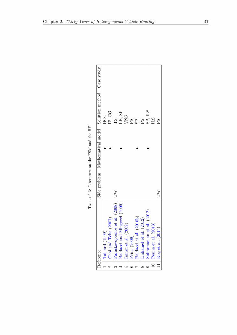
Chapter 2. Thirty Years of Heterogeneous Vehicle Routing 47
Table2.3:
Lit
eratu
reon
the
FS
Man
dth
eH
F
Ref
eren
ceS
ide
pro
ble
mM
ath
emat
ical
mod
elS
olu
tion
met
hod
Cas
est
ud
y
1T
aill
ard
(199
9)•
HC
G2
Ch
oian
dT
cha
(200
7)•
IP,
CG
3P
ara
skev
opou
los
etal
.(2
008)
TW
TS
4B
ald
acci
an
dM
ingo
zzi
(200
9)•
LB
,S
P5
Imra
net
al.
(2009
)V
NS
6P
rin
s(2
009)
PS
7B
ald
acci
etal.
(201
0b)
•S
P8
Du
ham
elet
al.
(201
2)P
S9
Su
bra
man
ian
etal
.(2
012)
•S
P,
ILS
10
Pen
na
etal.
(201
3)IL
S11
Koc
etal
.(2
015
)T
WP
S

Chapter 2. Thirty Years of Heterogeneous Vehicle Routing 48
We now present a comparison of the recent results for the FSM, HF and FSMTW in
Sections 2.8.2.1, 2.8.2.2 and 2.8.2.3, respectively.
2.8.2.1 Comparison of recent metaheuristics on the FSM
Table 2.4 presents a summary of the comparison results of recent metaheuristics for
the FSM with three costs variants, i.e., FSM(F,V), FSM(F) and FSM(V). For detailed
comparison results, the reader is referred to Tables A.1, A.2 and A.3 in the Appendix.
In these tables, the first column provides the references, and for each reference two
performance indicators are shown: the average percentage deviation (Dev) from the
value of the best-known solution (BKS) for each instance retrieved from the articles
surveyed, and the average computation time in seconds (Time). The reported running
times are the best solution running time over all runs. The computers and programming
languages used are not comparable, hence scaled times for one reference computer would
not be valid. We simply indicate the features of each computer such as processor and
CPU speed in GHz in the last column of the table.
Table 2.4 indicates an effective progress since 2007. All metaheuristics for the three cost
versions of the FSM achieve average deviations 0.2% or less. In terms solution quality,
the top performers are Penna et al. (2013) and Vidal et al. (2014) for the FSM(F,V),
Vidal et al. (2014) for the FSM(F), and Choi and Tcha (2007), Penna et al. (2013) and
Vidal et al. (2014) for the FSM(V).
2.8.2.2 Comparison of recent metaheuristics on the HF
Table 2.5 provides a summary of the average results of recent metaheuristics applied
to two costs variants of HF: HF(F,V) and HF(V). For detailed comparison results, the
reader is referred to Tables A.4 and A.5 in the Appendix.
Table 2.5 shows a continuous progress since 1999. Recent metaheuristics for all two cost
versions of the HF achieve average deviations 0.5% or less. In terms of solution quality,
the top performers are Subramanian et al. (2012) for the HF(F,V), and Li et al. (2007),
Subramanian et al. (2012), Liu (2013) and Penna et al. (2013) for the HF(V).

Chapter 2. Thirty Years of Heterogeneous Vehicle Routing 49
Table2.4:
Ave
rage
com
pari
son
of
rece
nt
met
ah
euri
stic
son
the
FS
M
Ref
eren
ceF
SM
(F,V
)F
SM
(F)
FS
M(V
)P
roce
ssor
CP
UD
ev(%
)T
ime
(s)
Dev
(%)
Tim
e(s
)D
ev(%
)T
ime
(s)
Ch
oi
and
Tch
a(2
007
)0.0
892
.70
0.08
150.
330.
0036
.06
Pen
tiu
mIV
2.6G
Hz
Bra
nd
ao
etal
.(2
009
)−
−0.
1019
1.83
0.02
294.
63P
enti
um
M1.
4GH
zIm
ran
etal.
(200
9)0.0
446
6.17
0.07
500.
500.
0253
1.00
Pen
tiu
mM
1.7G
Hz
Liu
etal.
(200
9)−
−0.
0319
8.17
0.04
260.
75P
enti
um
IV3G
Hz
Pri
ns
(2009
)0.0
223
.06
0.12
42.5
2−
−P
enti
um
IVM
1.8G
Hz
Pen
na
etal.
(201
3)0.0
024
.50
0.03
30.3
50.
0029
.77
Inte
li7
2.93
GH
zV
idal
etal.
(201
4)0.0
059
.30
0.01
68.1
00.
0051
.15
Op
t2.
4GH
z

Chapter 2. Thirty Years of Heterogeneous Vehicle Routing 50
Table2.5:
Ave
rage
com
pari
son
of
rece
nt
met
ah
euri
stic
son
the
HF
Ref
eren
ceH
F(F
,V)
HF
(V)
Pro
cess
orC
PU
Dev
(%)
Tim
e(s
)D
ev(%
)T
ime
(s)
Tail
lard
(1999
)−
−1.
2520
11.1
3S
un
Sp
arc
50M
Hz
Tara
nti
lis
etal.
(2004
)−
−0.
5160
7.13
Pen
tiu
mII
400M
Hz
Gen
cer
etal
.(2
006
)4.
63−
−−
−−
Li
etal.
(200
7)−
−0.
0328
5.75
AM
DA
thlo
n1.
0GH
zP
rin
s(2
009
)−
−0.
0694
.76
Pen
tiu
mIV
M1.
8GH
zL
iet
al.
(201
0)0.
2113
1.75
−−
Inte
l2.
2GH
zS
ub
ram
ania
net
al.
(201
2)0.
007.
730.
034.
03In
tel
i72.
93G
Hz
Liu
(201
3)0.
1912
7.05
0.03
71.1
7In
tel
Pen
tiu
mIV
3GH
zP
enn
aet
al.
(2013
)0.
0731
.97
0.03
31.8
9In
tel
i72.
93G
Hz

Chapter 2. Thirty Years of Heterogeneous Vehicle Routing 51
2.8.2.3 Comparison of recent metaheuristics on the FSMTW
Tables 2.6 and 2.7 present summaries of the results of recent metaheuristics for the
FSM on two costs variants: FSMTW(T) and FSMTW(D). The first column shows the
instance sets containing several instances. The second column shows the average BKS.
The remaining columns show, for each reference, the average percentage deviations of
each set, and the average solution time. The computer specifications are provided in the
last two rows.
In the case of the FSMTW(T), a continuous progress can be observed since 2007. Recent
metaheuristics, Vidal et al. (2014) and Koc et al. (2015), achieve average deviations
0.2% or less. In the case of the FSMTW(D), there has also been a significant progress
in terms of average deviations. Recent metaheuristics, Vidal et al. (2014) and Koc et
al. (2015), achieve average deviations of at most 0.1%. These two papers developed
powerful population search based metaheuristics, and obtained very effective results on
both cost variants of the FSMTW.
2.9 Conclusions and Future Research Directions
The Heterogeneous Vehicle Routing Problem (HVRP) was introduced some 30 years ago
by Golden et al. (1984) and has since evolved into a rich research area. Several versions
of the problem have been studied, and applications are encountered in many settings.
Our survey provides a classification of the HVRP literature under two main dimensions:
unlimited fleet and limited fleet. We have identified the following conclusions and future
research directions: 1) All five standard versions of the HVRP (FSM(F,V), FSM(F),
FSM(V), HF(F,V), HF(V)) have now been solved to near optimality by heuristics, and
it is our belief that this algorithmic research on the standard problems has now reached
maturity. 2) Over the years, most of the research effort has shifted towards the study of
rich extensions of the standard HVRP, such as time windows, multiple depots, external
carriers, pickup and delivery operations, container loading and bachauls. There still exist
numerous research opportunities on these rich extensions. 3) The “green” extension
of the problem has also received increasing attention in recent years. It would seem
interesting to study some extensions of the standard HVRP in a green context. 4)
Almost all studies, except one, have so far focused on time-independent versions of
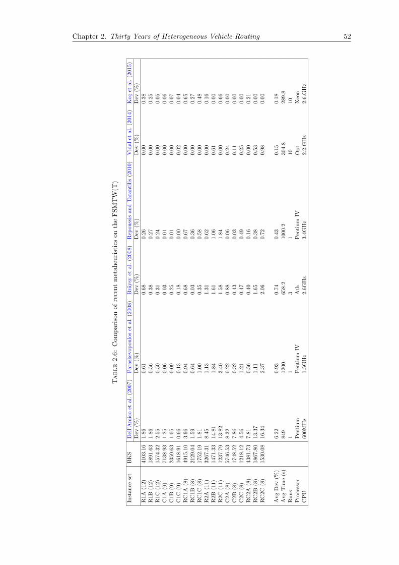
Chapter 2. Thirty Years of Heterogeneous Vehicle Routing 52
Table2.6:
Com
pari
son
of
rece
nt
met
ah
euri
stic
son
the
FS
MT
W(T
)
Inst
ance
set
BK
SD
ell’
Am
ico
etal
.(2
007)
Par
aske
vop
oulo
set
al.
(200
8)B
raysy
etal
.(2
008)
Rep
ouss
isan
dT
aran
tilis
(201
0)V
idal
etal.
(2014)
Koc
etal.
(2015)
Dev
(%)
Dev
(%)
Dev
(%)
Dev
(%)
Dev
(%)
Dev
(%)
R1A
(12)
4103
.16
1.86
0.61
0.68
0.26
0.00
0.3
8R
1B(1
2)18
91.6
31.
860.
560.
380.
270.
00
0.2
5R
1C(1
2)15
74.3
22.
550.
500.
310.
240.
00
0.0
5C
1A(9
)71
38.9
31.
250.
060.
030.
010.
00
0.0
6C
1B(9
)23
59.6
31.
050.
090.
250.
010.
00
0.0
7C
1C(9
)16
18.9
10.
660.
130.
180.
000.
02
0.0
4R
C1A
(8)
4915
.10
3.96
0.94
0.68
0.67
0.00
0.6
5R
C1B
(8)
2129
.04
1.59
0.64
0.03
0.36
0.00
0.2
7R
C1C
(8)
1752
.19
1.81
1.00
0.35
0.58
0.00
0.4
8R
2A(1
1)32
67.3
18.
451.
131.
310.
620.
00
0.1
6R
2B(1
1)14
71.3
314
.81
1.84
1.61
1.06
0.6
10.0
0R
2C(1
1)12
37.7
913
.82
3.40
1.58
1.84
0.0
00.6
6C
2A(8
)57
46.5
38.
320.
220.
880.
060.
24
0.0
0C
2B(8
)17
48.5
27.
860.
320.
430.
030.
11
0.0
0C
2C(8
)12
18.1
24.
561.
210.
470.
490.
25
0.0
0R
C2A
(8)
4381
.73
7.81
0.56
0.40
0.16
0.00
0.2
1R
C2B
(8)
1867
.80
13.3
71.
111.
650.
380.5
30.0
0R
C2C
(8)
1530
.08
16.3
42.
372.
060.
720.9
80.0
0
Avg
Dev
(%)
6.22
0.93
0.74
0.43
0.15
0.1
8A
vg
Tim
e(s
)84
912
0065
8.2
1000
.230
4.8
289.8
Ru
ns
11
31
10
10
Pro
cess
orP
enti
um
Pen
tiu
mIV
Ath
Pen
tiu
mIV
Op
tX
eon
CP
U60
0MH
z1.
5GH
z2.
6GH
z3.
4GH
z2.
2.G
Hz
2.6
.GH
z
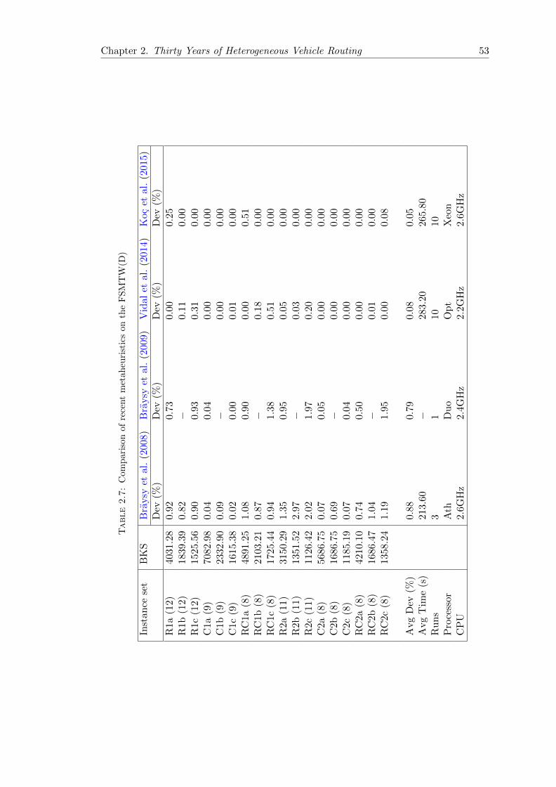
Chapter 2. Thirty Years of Heterogeneous Vehicle Routing 53
Table2.7:
Com
pari
son
of
rece
nt
met
ah
euri
stic
son
the
FS
MT
W(D
)
Inst
an
cese
tB
KS
Bra
ysy
etal
.(2
008)
Bra
ysy
etal
.(2
009)
Vid
alet
al.
(201
4)K
ocet
al.
(201
5)D
ev(%
)D
ev(%
)D
ev(%
)D
ev(%
)
R1a
(12)
4031
.28
0.92
0.73
0.00
0.25
R1b
(12)
1839
.39
0.82
−0.
110.
00R
1c(1
2)15
25.5
60.
900.
930.
310.
00C
1a
(9)
7082
.98
0.04
0.04
0.00
0.00
C1b
(9)
2332
.90
0.09
−0.
000.
00C
1c
(9)
1615
.38
0.02
0.00
0.01
0.00
RC
1a
(8)
4891
.25
1.08
0.90
0.00
0.51
RC
1b
(8)
2103
.21
0.87
−0.
180.
00R
C1c
(8)
1725
.44
0.94
1.38
0.51
0.00
R2a
(11)
3150
.29
1.35
0.95
0.05
0.00
R2b
(11)
1351
.52
2.97
−0.
030.
00R
2c(1
1)11
26.4
22.
021.
970.
200.
00C
2a
(8)
5686
.75
0.07
0.05
0.00
0.00
C2b
(8)
1686
.75
0.69
−0.
000.
00C
2c
(8)
1185
.19
0.07
0.04
0.00
0.00
RC
2a
(8)
4210
.10
0.74
0.50
0.00
0.00
RC
2b
(8)
1686
.47
1.04
−0.
010.
00R
C2c
(8)
1358
.24
1.19
1.95
0.00
0.08
Avg
Dev
(%)
0.88
0.79
0.08
0.05
Avg
Tim
e(s
)21
3.60
−28
3.20
265.
80R
un
s3
110
10P
roce
ssor
Ath
Du
oO
pt
Xeo
nC
PU
2.6G
Hz
2.4G
Hz
2.2G
Hz
2.6G
Hz

Chapter 2. Thirty Years of Heterogeneous Vehicle Routing 54
the HVRP. A more realistic version of the standard HVRP and its variants would be
to consider time-dependencies, particularly in urban settings and in city logistics. 5)
To our knowledge, no exact algorithm has yet been proposed for the FSMTW (except
for a simple branch-and-bound scheme) or the HFTW. Further studies should focus
on developing effective exact methods for those different problems. 6) HVRPs tend to
be very hard to solve, which explains why most algorithms are heuristics. These have
gradually evolved from simple interchange schemes to more sophisticated metaheuristics,
sometimes combining exact methods. In general, constructive heuristics complemented
with local search heuristics are the main methods of these studies, but researchers should
consider hybrid schemes combining population search and local search (like ALNS or
iterated local search), such as those applied to the standard VRP (Laporte et al. 2014).
Such metaheuristics should also be effective on special cases of FSM/HF and on problems
that contain FSM/HF as special cases. The recent tendency in the field of the VRP
heuristics has been to develop algorithms that are highly accurate but often require large
computing times and lack simplicity in the sense that they contain too many parameters
and are difficult to reproduce. This observation applies to most of the metaheuristics we
have just surveyed. While computing times have become more modest in some of the
best recent implementations, the lack of simplicity of these methods remains problematic
in many cases (Laporte et al. 2014). On a more positive note, we have witnessed in recent
years the emergence of flexible metaheuristics, based on genetic algorithm framework,
capable of solving a host of problem variants with the same parameter settings (Vidal
et al. 2014, Koc et al. 2015). 7) To our knowledge, only one study has developed a
continuous approximation model which is highly effective on the standard FSM. This
type of modelling should be applied to the HF and to rich extensions of the HVRP.
We believe this paper has helped unify the rapidly expanding body of knowledge on the
HVRP and will encourage other researchers to pursue the study of this fascinating field
of research.

Chapter 3
A Hybrid Evolutionary
Algorithm for Heterogeneous
Fleet Vehicle Routing Problems
with Time Windows
55
Chapter 3. A Hybrid Evolutionary Algorithm for Heterogeneous Fleet Vehicle RoutingProblems with Time Windows 56
Abstract
This paper presents a hybrid evolutionary algorithm (HEA) to solve heterogeneous fleet
vehicle routing problems with time windows. There are two main types of such problems,
namely the Fleet Size and Mix Vehicle Routing Problem with Time Windows (F) and
the Heterogeneous Fixed Fleet Vehicle Routing Problem with Time Windows (H), where
the latter, in contrast to the former, assumes a limited availability of vehicles. The main
objective is to minimize the fixed vehicle cost and the distribution cost, where the latter
can be defined with respect to en-route time (T) or distance (D). The proposed unified
algorithm is able to solve the four variants of heterogeneous fleet routing problem, called
FT, FD, HT and HD, where the last variant is new. The HEA successfully combines
several metaheuristics and offers a number of new advanced efficient procedures tailored
to handle the heterogeneous fleet dimension. Extensive computational experiments on
benchmark instances have shown that the HEA is highly effective on FT, FD and HT.
In particular, out of the 360 instances we obtained 75 new best solutions and matched
102 within reasonable computational times. New benchmark results on HD are also
presented.
Keywords. vehicle routing; time windows; heterogeneous fleet; genetic algorithm; neigh-
borhood search
3.1 Introduction
In heterogeneous fleet vehicle routing problems with time windows, one considers a fleet
of vehicles with various capacities and vehicle-related costs, as well as a set of customers
with known demands and time windows. These problems consist of determining a set
of vehicle routes such that each customer is visited exactly once by a vehicle within a
prespecified time window, all vehicles start and end their routes at a depot, and the load
of each vehicle does not exceed its capacity. As is normally the case in vehicle routing
problem with time windows (VRPTW), customer service must start within the time
window, but the vehicle may wait at a customer location if it arrives before the beginning
of the time window. There are two main categories of such problems, namely the Fleet
Size and Mix Vehicle Routing Problem with Time Windows (F) and the Heterogeneous
Fixed Fleet Vehicle Routing Problem with Time Windows (H). In category F, there is

Chapter 3. A Hybrid Evolutionary Algorithm for Heterogeneous Fleet Vehicle RoutingProblems with Time Windows 57
no limit in the number of available vehicles of each type, whereas such a limit exists in
category H. Note that it is easy to find feasible solutions to the instances of category F
since there always exists a feasible assignment of vehicles to routes. However, this is not
always the case for the instances of category H.
Two measures are used to compute the total cost to be minimized. The first is the sum
of the fixed vehicle cost and of the en-route time (T), which includes traveling time and
possible waiting time at the customer locations before the opening of their time windows
(we assume that travel time and cost are equivalent). In this case, service times are only
used to check feasibility and for performing adjustments to the departure time from the
depot in order to minimize pre-service waiting times. The second cost measure is based
on distance (D) and consists of the fixed vehicle cost and the distance traveled by the
vehicle, as is the case in the standard VRPTW (Solomon 1987).
We differentiate between four variants defined with respect to the problem category
and to the way in which the objective function is defined, namely FT, FD, HT and
HD. The first variant is FT, described by Liu and Shen (1999b) and the second is FD,
introduced by Braysy et al. (2008). The third variant HT was defined and solved by
Paraskevopoulos et al. (2008). Finally, HD is a new variant which we introduce in this
paper. HD differs from HT by considering the objective function D instead of T. This
variant has never been studied before.
Hoff et al. (2010) and Belfiore and Yoshizaki (2009) describe several industrial aspects
and practical applications of heterogeneous vehicle routing problems. The most studied
versions are the fleet size and mix vehicle routing problem, described by Golden et al.
(1984), which considers an unlimited heterogeneous fleet, and the heterogeneous fixed
fleet vehicle routing problem, proposed by Taillard (1999). For further details, the reader
is referred to the surveys of Baldacci et al. (2008) and of Baldacci et al. (2009).
The FT variant has several extensions, e.g., multiple depots (Dondo and Cerda 2007, Bet-
tinelli et al. 2011), overloads (Kritikos and Ioannou 2013), and split deliveries (Belfiore
and Yoshizaki 2009, 2013). There exist several exact algorithms for the capacitated
vehicle routing problem (VRP) (Toth and Vigo 2002, Baldacci et al. 2010a), and for the
heterogeneous VRP (Baldacci et al. 2009). However, to the best of our knowledge, no
exact algorithm has been proposed for the heterogeneous VRP with time windows, i.e.,

Chapter 3. A Hybrid Evolutionary Algorithm for Heterogeneous Fleet Vehicle RoutingProblems with Time Windows 58
FT, FD and HT. The existing heuristic algorithms for these three variants are briefly
described below.
Liu and Shen (1999b) proposed a heuristic for FT which starts by determining an ini-
tial solution through an adaptation of the Clarke and Wright (1964) savings algorithm,
previously presented by Golden et al. (1984). The second stage improves the initial
solution by moving customers by means of parallel insertions. The algorithm was tested
on a set of 168 benchmark instances derived from the set of Solomon (1987) for the
VRPTW. Dullaert et al. (2002) described a sequential construction algorithm for FT,
which is an extension of the insertion heuristic of Golden et al. (1984). Dell’Amico et
al. (2007) described a multi-start parallel regret construction heuristic for FT, which
is embedded into a ruin and recreate metaheuristic. Braysy et al. (2008) presented a
deterministic annealing metaheuristic for FT and FD. In a later study, Braysy et al.
(2009) described a hybrid metaheuristic algorithm for large scale FD instances. Their
algorithm combines the well-known threshold acceptance heuristic with a guided local
search metaheuristic having several search limitation strategies. An adaptive memory
programming algorithm was proposed by Repoussis and Tarantilis (2010) for FT, which
combines a probabilistic semi-parallel construction heuristic, a reconstruction mecha-
nism and a tabu search algorithm. Computational results indicate that their method
is highly successful and improves many best known solutions. In a recent study, Vidal
et al. (2014) introduced a genetic algorithm based on a unified solution framework for
different variants of the VRPs, including FT and FD. To our knowledge, Paraskevopou-
los et al. (2008) are the only authors who have studied HT. Their two-phase solution
methodology is based on a hybridized tabu search algorithm capable of solving both FT
and HT.
This brief review shows that the two problem categories F and H have already been
solved independently through different methodologies. We believe there exists merit for
the development of a unified algorithm capable of efficiently solving the two problem
categories. This is the main motivation behind this paper.
This paper makes three main scientific contributions. First, we develop a unified hybrid
evolutionary algorithm (HEA) capable of handling the four variants of the problem. The
HEA combines two state-of-the-art metaheuristic concepts which have proved highly suc-
cessful on a variety of VRPs: Adaptive Large Neighborhood Search (ALNS) (see Ropke

Chapter 3. A Hybrid Evolutionary Algorithm for Heterogeneous Fleet Vehicle RoutingProblems with Time Windows 59
and Pisinger 2006a, Pisinger and Ropke 2007, Demir et al. 2012) and population based
search (see Prins 2004, Vidal et al. 2014). The second contribution is the introduction
of several algorithmic improvements to the procedures developed by Prins (2009) and
Vidal et al. (2012). We use a ALNS equipped with a range of operators as the main
Education procedure within the search. We also propose an advanced version of the
Split algorithm of Prins (2009) capable of handling infeasibilities. Finally, we introduce
an innovative aggressive Intensification procedure on elite solutions, as well as a new
diversification scheme through the Regeneration and the Mutation procedures of
solutions. The third contribution is to introduce HD as a new problem variant.
The remainder of this paper is structured as follows. Section 3.2 presents a detailed
description of the HEA. Computational experiments are presented in Section 3.3, and
conclusions are provided in Section 3.4.
3.2 Description of the Hybrid Evolutionary Algorithm
We start by introducing the notation related to FT, FD, HT and HD. All problems are
defined on a complete graph G = (N ,A), where N = 0, . . . , n is the set of nodes, and
node 0 corresponds to the depot. Let A = (i, j) : 0 ≤ i, j ≤ n, i 6= j denote the set
of arcs. The distance from i to j is denoted by dij . The customer set is Nc in which
each customer i has a demand qi and a service time si, which must start within time
window [ai, bi]. If a vehicle arrives at customer i before ai, it then waits until ai. Let
K = 1, . . . , k be the set of available vehicle types. Let ek and Qk denote the fixed
vehicle cost and the capacity of vehicle type k, respectively. The travel time from i to
j is denoted by tij and is independent of the vehicle type. The distribution cost from i
to j associated with a vehicle of type k is ckij for all problem types. In HT and HD, the
available number of vehicles of type k ∈ K is nk, whereas the constant can be set to an
arbitrary large value for problems FT and FD. The objectives are as discussed in the
Introduction.
The remainder of this section introduces the main components of the HEA. A gen-
eral overview of the HEA is given in Section 3.2.1. More specifically, Section 3.2.2
presents the offspring Education procedure. Section 3.2.3 presents the initialization of
the population. The selection of parent solutions, the ordered crossover operator and

Chapter 3. A Hybrid Evolutionary Algorithm for Heterogeneous Fleet Vehicle RoutingProblems with Time Windows 60
the advanced algorithm Split are described in Sections 3.2.4, 3.2.5 and 3.2.6, respec-
tively. Section 3.2.7 presents the Intensification procedure. The survivor selection
mechanism is detailed in Section 3.2.8. Finally, the diversification stage, including the
Regeneration and Mutation procedures, is described in Section 3.2.9.
3.2.1 Overview of the hybrid evolutionary algorithm
The HEA brings together the well-known components of evolutionary algorithms, such
as parent selection and crossover, some advanced operators to educate, intensify and
diversify the population. The Split procedure is applied on a giant tour obtained from
combining two parents in the population, the quality which is further improved by a
quality of ALNS. Further details on the components are explained below.
The general structure of the HEA is presented in Algorithm 1. The modified version of
the classical Clarke and Wright savings algorithm and the ALNS operators are combined
to generate the initial population (Line 1). Two parents are selected (Line 3) through
a binary tournament, following which the crossover operation (Line 4) generates a new
offspring C.
The advanced Split algorithm is applied to the offspring C (Line 5), which optimally
segments the giant tour by choosing the vehicle type for each route. This algorithm
is a tour splitting procedure which optimally partitions a solution into feasible routes.
Each solution is a permutation of customers without trip delimiters and can therefore
be viewed as a giant TSP tour for a vehicle with a large enough capacity.
The Education procedure (Line 6) uses the ALNS operators to educate offspring C
and inserts it back into the population. If C is infeasible, the Education procedure is
iteratively applied until a modified version of C is feasible, which is then inserted into
the population. The probabilities associated with the operators used in the Education
procedure and the penalty parameters are updated by means of an adaptive weight
adjustment procedure (AWAP) (Line 7).
At each iteration of the algorithm, all individuals in the population are ranked in de-
creasing order solution cost. The first ne individuals of this ranking are called elite
solutions which are carried over to the next iteration. Elite solutions are put through an

Chapter 3. A Hybrid Evolutionary Algorithm for Heterogeneous Fleet Vehicle RoutingProblems with Time Windows 61
aggressive Intensification procedure, based on the ALNS algorithm (Line 8) in order
to improve their quality.
If, at any iteration, the population size na reaches np + no, then a survivor selection
mechanism is applied (Line 9). The population size, shown by na, changes during the
algorithm as new offsprings are added, but is limited by np +no, where np is a constant
denoting the size of the population initialized at the beginning of the algorithm and no
is a constant showing the maximum allowable number of offsprings that can be inserted
into the population. At each iteration of the algorithm, Mutation is applied to a
randomly selected individual from the population with probability pm. If there are no
improvements in the best known solution for a number of consecutive iterations itr, the
entire population undergoes a Regeneration (Line 10). The HEA terminates when
the number of iterations without improvement itt is reached (Line 11).
Algorithm 1 The general framework of the HEA
1: Initialization: initialize a population with size np2: while number of iterations without improvement < itt do3: Parent selection: select parent solutions P1 and P2
4: Crossover : generate offspring C from P1 and P2
5: Split: partition C into routes6: Education: educate C with ALNS and insert into population7: AWAP : update probabilities of the ALNS operators8: Intensification: intensify elite solution with ALNS9: Survivor selection: if the population size na reaches np+no, then select survivors
10: Diversification: diversify the population with Mutation or Regeneration pro-cedures
11: end while12: Return best feasible solution
3.2.2 Education
The Education procedure is systematically applied to each offspring in order to improve
its quality. The ALNS algorithm is used as a way of educating the solutions in the
HEA. This is achieved by applying both the destroy and repair operators, and a number
of removable nodes are modified in each iteration. An example of the removal and
insertion phases is illustrated in Figure 3.1. The operators used within the HEA are
either adapted or inspired from those employed by various authors (Ropke and Pisinger
2006a,b, Pisinger and Ropke 2007, Demir et al. 2012, Paraskevopoulos et al. 2008).

Chapter 3. A Hybrid Evolutionary Algorithm for Heterogeneous Fleet Vehicle RoutingProblems with Time Windows 62
Dep
ot
8
2
10
3
4
11
5
71
96
Dep
ot
8
2
10
3
4
11
5
71
96
Dep
ot
8
2
10
3
4
11
5
71
96
a:
A f
easi
ble
so
luti
on
b:
A d
estr
oy
ed s
olu
tio
n
c:A
rep
aire
d s
olu
tio
n
Lr
=
Lr
=
7,2
,3
L
r=
Figure3.1:
Illu
stra
tion
of
theEducation
pro
ced
ure

Chapter 3. A Hybrid Evolutionary Algorithm for Heterogeneous Fleet Vehicle RoutingProblems with Time Windows 63
The Education procedure is detailed in Algorithm 2. All operators are repeated O(n)
times and the complexity given are the overall repeats. The removal procedure (line 4 of
Algorithm 2) runs for n′ iterations, removes n′ customers from the solution and add to
the removal list Lr, where n′ is in the interval of removable nodes [bel , beu]. An insertion
operator is then selected to iteratively insert the nodes, starting from the first customer
of Lr, into the partially destroyed solution until Lr is empty (line 5). The feasibility
conditions in terms of capacity and time windows for FT, FD, HT and HD, and in terms
of fleet size for HT and HD, are always respected during the insertion process. We do
not allow overcapacity of the vehicle and service start outside the time windows for all
problem types, and we also do not allow the use of additional vehicles beyond the fixed
fleet size for HT and HD. The removal and insertion operators are randomly selected
according to their past performance and a certain probability as explained further in
Section 3.2.2.3. The cost of an individual C before the removal is denoted by ω(C), and
its cost after the insertion is denoted by ω(C∗).
Algorithm 2 Education
1: Initialize: An individual C, ω(C)← cost of C, ω(C∗)← 0, iteration ← 02: while there is no improvement and C is feasible do3: Lr = ∅ and select a removal operator4: Apply a removal operator to the individual C to remove a set of nodes and add
them to Lr5: Select an insertion operator and apply it to the partially destroyed individual C
to insert the nodes of Lr6: Let C∗ be the new solution obtained by applying insertion operator7: if ω(C∗) < ω(C) and C∗ is feasible then8: ω(C)← ω(C∗)
9: iteration ← iteration + 110: end while11: Return educated feasible solution
The heterogeneous fleet version of the ALNS that we use here was recently introduced
in Chapter 5. It educates solutions by considering the heterogeneous fleet aspect. The
ALNS integrates fleet sizing within the destroy and repair operators. In particular, if
a node is removed, we check whether the resulting route can be served by a smaller
vehicle. We then update the solution accordingly. If inserting a node requires additional
vehicle capacity we then consider the option of using larger vehicles. For each node
i ∈ Nc\Lr, let fh(i) be the current vehicle fixed cost associated with the vehicle serving
i. Let ∆(i) be the saving obtained as a result of using a removal operator on node
i without considering the vehicle fixed cost. Let fh∗1 (i) be the vehicle fixed cost after

Chapter 3. A Hybrid Evolutionary Algorithm for Heterogeneous Fleet Vehicle RoutingProblems with Time Windows 64
removal of node i. Consequently, fh∗1 (i) < fh(i) only if the route containing node i can
be served by a smaller vehicle when removing node i. The savings in vehicle fixed cost
can be expressed as fh(i) − fh∗1 (i), respectively. Thus, for each removal operator, the
total savings of removing node i ∈ Nc\Lr, denoted RC(i), is calculated as follows:
RC(i) = ∆(i) + (fh(i)− fh∗1 (i)). (3.1)
In a destroyed solution, the insertion cost of node j ∈ Lr after node i is defined as Ω(i, j)
for a given node i ∈ Nc\Lr. Let fh∗2 (i) be the vehicle fixed cost after the insertion of
node i, i.e., fh∗2 > fh only if the route containing node i necessitates the use of a larger
capacity vehicle after inserting node i. The cost differences in vehicle fixed cost can be
expressed as fh∗2 (i) − fh(i). Thus, the total insertion cost of node i ∈ Nc\Lr, for each
insertion operator is
IC(i) = Ω(i, j) + (fh∗2 (i)− fh(i)). (3.2)
3.2.2.1 Removal operators
Nine removal operators are used in the destroy phase of the Education procedure and
are described in detail below. The first eight were used in several papers (Ropke and
Pisinger 2006a,b, Demir et al. 2012, Koc et al. 2015), whereas the last one is new. We
introduce the ninth one as a new removal operator specific to FT, FD HT and HD.
1.Random removal (RR): The RR operator randomly selects a node j ∈ N\0\Lr,
removes it from the solution.
2.Worst distance removal (WDR): The purpose of the WDR operator is to choose a
number of expensive nodes according to their distance based cost. The cost of a node
j ∈ N\0\Lr is the distance from its predecessor i and its distance to its successor
k. The WDR operator iteratively removes nodes j∗ from the solution where j∗ =
arg maxj∈N\0\Lrdij + djk + fh(i)− fh∗1 (i).
3.Worst time removal (WTR): The WTR operator is a variant of the WDR operator. For
each node j ∈ N\0\Lr costs are calculated, depending on the deviation between the
arrival time zj and the beginning of the time window aj . The WTR operator iteratively
removes customers from the solution, where j∗ = arg maxj∈N\0\Lr|zj − aj |+ fh(i)−
fh∗1 (i). The ALNS iteratively applies this process to the solution after each removal.

Chapter 3. A Hybrid Evolutionary Algorithm for Heterogeneous Fleet Vehicle RoutingProblems with Time Windows 65
4.Neighborhood removal (NR): In a given solution with a set < of routes, the NR operator
calculates an average distance d(R) =∑
(i,j)∈R dij/|R| for each route R ∈ <, and selects
a node j∗ = arg max(R∈<;j∈R)d(R)− dR\j+ fh(i)− fh∗1 (i), where dR\j denotes the
average distance of route R excluding node j.
5. Shaw removal (SR): The general idea behind the SR operator, which was introduced
by Shaw (1998), is to remove a set of customers that are related in a predefined way and
are therefore easy to change. The SR operator removes a set of n′ similar customers.
The similarity between two customers i and j is defined by the relatedness measure
δ(i, j). This includes four terms: a distance term dij , a time term |ai − aj |, a relation
term lij , which is equal to −1 if i and j are in the same route, and 1 otherwise, and a
demand term |qi − qj |. The relatedness measure is given by
δ(i, j) = ϕ1dij + ϕ2|ai − aj |+ ϕ3lij + ϕ4|qi − qj |, (3.3)
where ϕ1 to ϕ4 are weights that are normalized to find the best candidate solution.
The operator starts by randomly selecting a node i ∈ N\0\Lr, and selects the node
j∗ to remove where j∗ = arg minj∈N\0\Lrδ(i, j) + fh(i) − fh∗1 (i). The operator is
iteratively applied to select a node which is most similar to the one last added to Lr.
6. Proximity-based removal (PBR): This operator is a second variant of the classical
Shaw removal operator. The selection criterion of a set of routes is solely based on the
distance. Therefore, the weights are ϕ1 = 1 and ϕ2 = ϕ3 = ϕ4 = 0.
7. Time-based removal (TBR): The TBR operator removes a set of nodes that are
related in terms of time. It is a special case of the Shaw removal operator where ϕ2 = 1
and ϕ1 = ϕ3 = ϕ4 = 0.
8. Demand-based removal (DBR): The DBR operator is yet another variant of the Shaw
removal operator with ϕ4 = 1 and ϕ1 = ϕ2 = ϕ3 = 0.
9. Average cost per unit removal (ACUTR): The average cost per unit (ACUT) is
described by Paraskevopoulos et al. (2008) to measure the utilization efficiency of a
vehicle Π(R) on a given route R. Π(R) is expressed as the ratio of the total travel cost
and fixed vehicle cost over the total demand carried by a vehicle k traversing route R:
Π(R) =
∑(i,j)∈A cijx
kij + ek∑
i∈N\0 qixkij
. (3.4)

Chapter 3. A Hybrid Evolutionary Algorithm for Heterogeneous Fleet Vehicle RoutingProblems with Time Windows 66
The aim of the ACUTR operator is to calculate the cost of each route and remove the
one with the least Π(R) value from the solution.
3.2.2.2 Insertion operators
Three insertion operators are used in the repair phase of the Education procedure.
The first two were used in several papers (Ropke and Pisinger 2006a,b, Demir et al.
2012, Koc et al. 2015), whereas the last one is new. We introduce the third one as a
new insertion operator specific to FT and HT.
1. Greedy insertion (GI): The aim of this operator is to find the best possible insertion
position for all nodes in Lr. For node i ∈ N\Lr succeeded in the destroyed solution
by k ∈ N\0\Lr, and node j ∈ Lr we define γ(i, j) = dij + djk − dik. We find the
least-cost insertion position for j ∈ Lr by i∗ = arg mini∈N\Lrγ(i, j) + fh∗2 (i)− fh(i).
This process is iteratively applied to all nodes in Lr.
2. Greedy insertion with noise function (GINF): The GINF operator is based on the GI
operator but extends it by allowing a degree of freedom in selecting the best place for a
node. This is done by calculating the noise cost υ(i, j) = γ(i, j)+fh∗2 (i)−fh(i)+dmaxpnεij
where dmax is the maximum distance between all nodes, pn is a noise parameter used
for diversification and is set equal to 0.1, and εij is a random number in [−1, 1] for
i ∈ N\Lr, j ∈ Lr.
3. Greedy insertion with en-route time (GIET): This operator calculates the en-route
time difference η(i, j) between before and after inserting the customer j ∈ Lr. For node
i ∈ N\Lr succeeded in the destroyed solution by k ∈ N\0\Lr, and node j ∈ Lr, we
define η(i, j) = τij+τjk−τik where τij is the en-route time from node i to node j. We find
the least-cost insertion position for j ∈ Lr by i∗ = arg mini∈N\Lrη(i, j) + fh∗2 (i)− fh(i).
3.2.2.3 Adaptive weight adjustment procedure
Each removal and insertion operator has a certain probability of being chosen in every
iteration. The selection criterion is based on the historical performance of every operator
and is calibrated by a roulette-wheel mechanism (Ropke and Pisinger 2006a, Demir et
al. 2012). After itw iterations of the roulette wheel segmentation, the probability of each

Chapter 3. A Hybrid Evolutionary Algorithm for Heterogeneous Fleet Vehicle RoutingProblems with Time Windows 67
operator is recalculated according to its total score. Initially, the probabilities of each
removal and insertion operator are equal. Let pti be the probability of operator i in the
last itw iterations, pt+1i = pti(1− rp)+rpπi/τi, where rp is the roulette wheel probability,
for operator i ; πi is its score and τi is the number of times it was used during the last
segment. At the start of each segment, the scores of all operators are set to zero. The
scores are changed by σ1 if a new best solution is found, by σ2 if the new solution is
better than the current solution and by σ3 if the new solution is worse than the current
solution.
3.2.3 Initialization
The procedure used to generate the initial population is based on a modified version of
the Clarke and Wright and ALNS algorithms. An initial individual solution is obtained
by applying Clarke and Wright algorithm and by selecting the largest vehicle type for
each route. Then, until the initial population size reaches np, new individuals are created
by applying to the initial solution operators based on random removals and greedy
insertions with a noise function (see Section 3.2.2). We have selected these two operators
in order to diversify the initial population. The number of nodes removed is randomly
chosen from the initialization interval [bil, biu], which is defined by a lower and an upper
bound calculated as a percentage of the total number of nodes in an instance.
3.2.4 Parent selection
In evolutionary algorithms, the evaluation function of individuals is often based on
the solution cost. However, this kind of evaluation, does not take into account other
important factors such as the diversity of the population which plays a critical role. Vidal
et al. (2012) proposed a new method, named biased fitness bf(C), to tackle this issue.
This method considers the cost of an individual C, as well as its diversity contribution
dc(C) to the population. This function is continuously updated and is used to measure
the quality of individuals during selection phases. The dc(C) is defined as
dc(C) =1
nc
∑C′∈Nc
β(C,C ′), (3.5)

Chapter 3. A Hybrid Evolutionary Algorithm for Heterogeneous Fleet Vehicle RoutingProblems with Time Windows 68
where Nc is the set of the nc closest neighbours of C in the population. Thus, dc(C)
calculates the average distance between C and its neighbours in Nc. The distance
between two parents β(C,C ′) is the number of pairs of adjacent requests in C which
are no longer adjacent, (called broken), in C ′. For example, let C = 4, 5, 6, 7, 8, 9, 10
and C ′ = 10, 7, 8, 9, 5, 6, 4, in C ′ the pairs 4, 5, 6, 7 and 9, 10 are broken and
β(C,C ′) = 3. The algorithm selects the broken pairs distance (see Prins 2009) to
compute the distance β. The main idea behind dc(C) is to assess the differences between
individuals.
The evaluation function of an individual C in a population is
bf(C) = rc(C) + (1− nena
)rdc(C), (3.6)
which is based on the rank rc(C) of solution cost, and on the rank rdc(C) of the diver-
sity contribution. The rank rdc(C) is based on the diversity contribution calculated in
equation (3.5), according to which the solutions are ranked in decreasing order of their
dc(C) value. In (3.6), ne is the number of elite individuals and na is the current number
of individuals.
The HEA selects two parents through a binary tournament to yield an offspring. The
selection process randomly chooses two individuals from the population and keeps the
one having the best biased fitness.
3.2.5 Crossover
Two parents undergo the classical Ordered Crossover or OX without trip delim-
iters, following the parent selection phase. The OX operator is well suited for cyclic
permutations, and the giant tour encoding allows recycling crossovers designed for the
traveling salesman problem (TSP) (see Prins 2004, 2009). Initially, two positions i and
j are randomly selected in the first parent P1. Subsequently, the substring (i, ..., j) is
copied into the first offspring O1, at the same positions. The second parent P2 is then
swept cyclically from position j + 1 until the last node of P2, and continues from the
first node of P2 and continue until position i − 1, such that empty positions in O1 are
filled. The second offspring O2 is generated likewise by exchanging the roles of P1 and
P2. In the original version of OX, two offsprings are obtained. However in the HEA,

Chapter 3. A Hybrid Evolutionary Algorithm for Heterogeneous Fleet Vehicle RoutingProblems with Time Windows 69
we only randomly select one offspring. Figure 3.2 shows an illustration of Ordered
Crossover.
P1
P2
1 2 3 4 5 6 7 98
3 16 5 4 27 8 9
1 2 3 4 5 6 7 98
6 98 2 1 43 5 7
i j
O1
O2
1 2 3 4 5 6 7 98
2 61 5 4 97 8 3
1 2 3 4 5 6 7 98
8 64 2 1 93 5 7
Figure 3.2: Illustration of Ordered Crossover
3.2.6 Split algorithm
This algorithm was successfully applied in evolutionary based algorithms for several
routing problems (Prins 2004, 2009, Vidal et al. 2012, 2013). We propose an advanced
tour splitting procedure, denoted by Split, which is embedded in the HEA to segment
a giant tour and to determine the fleet mix composition. This is achieved through a
controlled exploration of infeasible solutions (see Cordeau et al. 2001 and Nagata et al.
2010), by relaxing the limits on time windows and vehicle capacities. Violations of these
limits are penalized through an objective function containing extra terms to acccount for
infeasibilities. This is in contrast to Prins (2009) who does not allow infeasibilities, and
in turn solves a resource-constrained shortest path problem using dynamic programming
to determine the best fleet mix on a given solution. Our implementation also differs from
those of Vidal et al. (2013) since it allows for infeasibilities that are not just related to
time windows or load, but also to the fleet size in the case of HT and HD.
We now describe the Split algorithm. Let < be the set of all routes in individual C, and
let R be a route. While formally R is a vector, for convenience we denote the number of
its components by |R|. Therefore, R = (i0 = 0, i1, i2, . . . , i|R|−1, i|R| = 0), we also write

Chapter 3. A Hybrid Evolutionary Algorithm for Heterogeneous Fleet Vehicle RoutingProblems with Time Windows 70
i ∈ R if i is a component of R, and (i, j) ∈ R if i and j appear in succession in R. Let
zt be the arrival time at the tth customer in R, thus the time window violation of route
R is∑|R|−1
t=1 maxzt − bit , 0. The total load for route R is∑|R|−1
t=1 qit , and we consider
solutions with a total load not exceeding twice the capacity of the largest vehicle given
by Qmax (Vidal et al. 2013). Furthermore, for route R and for each vehicle type k we
compute y(k), which is the number of vehicles of type k used in the solution.
Let λt, λl and λf represent the penalty values for any violations of the time windows,
the vehicle capacity and the fleet size, respectively. The variable xkij is equal to 1 if
customer i immediately precedes customer j visited by vehicle of type k. The fixed cost
associated with using a vehicle of type k ∈ K is denoted by ek. For each route R ∈ <
traversed by vehicle k ∈ K, the cost including penalties is
ν(R, k) =∑
(i,j)∈R
ckijxkij +ek+λt
|R|−1∑t=1
maxzt− bit , 0+λlmax|R|−1∑t=1
qit−Qmax, 0, (3.7)
which brings various objectives together to be able to guide to the search towards infea-
sible solutions. Thus, the total cost of individual C is
∆(C) =∑R∈<
∑k∈K
ν(R, k) + λf∑k∈K
max0, y(k)− nk, (3.8)
where nk is set equal to a sufficiently large number (e.g., n) for FT and FD, in order for
the last term in Equation (3.8) to be zero.
The Split operator works on a graph G′ = (N ,A′) where N = v0, v1, v2, . . . , vn
is an ordered set of nodes in which v0 = 0 and v1, v2, . . . , vn is the order of cus-
tomer nodes visited in the giant tour. The set of arcs in G′ is defined by A′ =
(vi, vj)|vi ∈ N , vj ∈ N , vj > vi, where each arc (vi, vj) ∈ A′ corresponds to a route
R = 0, vi+1, vi+2, . . . , vj , 0 in <. The cost of route R is calculated as explained above.
The Split procedure solves a shortest path problem on graph G′ from source node 0 to
destination node vn, where the arcs that appear on the shortest path correspond to the
partitioning of the new routes in individual C.
Figure 3.3 shows the steps of this advanced procedure applied to an FD instance. The arc
costs, demands and time windows are given in Figure 3.3.a. In particular, the number in
bold within the parentheses associated with each node is the demand for that customer;

Chapter 3. A Hybrid Evolutionary Algorithm for Heterogeneous Fleet Vehicle RoutingProblems with Time Windows 71
Depot1
2
45
3Depot
1
2
45
3
0 1 2 3 4 5
6 6
6
5
15 25
30
10
10
20
2025
15
97
56
10
15
30 40
71
40 65 60
74
173
a: The giant tour c: The optimal partition into
routes and vehicles
b: The arcs of the shortest path solution and Graph H
Type 2
Type 1
Type 3
Type 1
Type 1
Type 2
Type 2
Type 3
Type 2
Type 1
(12) [4,15]
(15) [30,50]
(7) [13,50]
(8) [2,20]
(11) [45,65]
(9) [2,7]
10
Figure 3.3: Illustration of procedure Split
the two numbers within brackets define the time window. Service times are identical
and equal to 4 for each customer, and three different types of vehicles are available. The
capacity qk and fixed cost ek of vehicles of type 1,2,3 are q1 = 10, q2 = 20, q3 = 30
and e1 = 6, e2 = 8, e3 = 10, respectively. The algorithm starts with a giant TSP tour
which includes six customers and uses one vehicle with unlimited capacity. The Split
algorithm computes an optimal compound segmentation in three routes corresponding
to three sequences of customers 1,2, 3,4,5 and 6 with three vehicle choices, Type
2, Type 3 and Type 1, respectively, as shown in Figure 3.3.b. The resulting solution is
shown in Figure 3.3.c. An optimal partitioning of the giant tour into routes for offspring
C corresponds to a minimum-cost path.
The penalty parameters of the Split algorithm are initially set to an initial value and are
dynamically adjusted during the algorithm. If an individual is still infeasible after the

Chapter 3. A Hybrid Evolutionary Algorithm for Heterogeneous Fleet Vehicle RoutingProblems with Time Windows 72
first Education procedure, then the penalty parameters are multiplied by λm and the
Education procedure restarts. When this solution becomes feasible, the parameters
are reset to their initial values. These values are λt = λl = λf = 3, λm = 10.
3.2.7 Intensification
We introduce a two-phase aggressive Intensification procedure to improve the quality
of elite individuals. This procedure intensifies the search within promising regions of the
solution space. The detailed pseude-code of this method is shown in Algorithm 3. The
algorithm starts with an elite list of solutions Le, which takes the best ne individuals
from the main population as measured by equation (3.6). Step 1 is similar to the main
Education procedure (Section 3.2.2). Step 2 attempts to explore different regions of
the search space with the RR operator, intensifies this area by applying the GI operator
for FD and HD, and GIET for FT and HT, to a partially destroyed solution. Steps 1 and
2 terminate when there is no improvement to the solution and the main loop terminates
when ne successive iterations have been performed.
Due to the difficulty of the problems considered in this paper, we have developed a two-
phase aggressive Intensification procedure after having tried several variants such as
one-phase with only Step 1 or Step 2, three-phase with Step 1, Step 2 and Step 1 and
various other combinations.
3.2.8 Survivor selection
In population-based metaheuristics, avoiding premature convergence is a key challenge.
Ensuring the diversity of the population, in other words to search a different location in
the solution space during the algorithm, in the hope of being closer to the best known
or optimal solutions constitutes a major trade-off between solutions in a population.
The method of Vidal et al. (2012), aims to ensure the diversity of the population and
preserve the elite solutions. The second part of this method is the survivor selection
process (the first part was discussed in Section 3.2.4). In this way, elite individuals are
protected.

Chapter 3. A Hybrid Evolutionary Algorithm for Heterogeneous Fleet Vehicle RoutingProblems with Time Windows 73
Algorithm 3 Intensification
1: Initialize Le = χ1, . . . , χn, i← 12: while all elite solutions are intensified do3: χ← χi4: Step 15: while there is improvement and elite solution χ is feasible do6: Lr = ∅ and select a removal operator7: Apply to the elite solution χ to remove nodes and add them to Lr8: Select an insertion operator and apply it to the destroyed elite solution χ by
inserting the node of Lr9: Let χ∗ be the new solution obtained by applying insertion operator
10: if ω(χ∗) < ω(χ) then11: ω(χ)← ω(χ∗)
12: end while13: Step 214: while there is improvement and χ∗ is feasible do15: Lr = ∅ and apply RR operator to the elite solution χ to remove nodes and
add them to Lr16: Apply GI or GIET operator to the partially destroyed elite solution χ by
inserting the node of Lr17: Let χ∗ be the new elite solution obtained by applying insertion operator18: if ω(χ∗) < ω(χ) then19: ω(χ)← ω(χ∗)
20: end while21: i← i+ 122: end while23: Return elite solutions
3.2.9 Diversification
The efficient management of feasible solutions plays a significant role in population
diversity. The performance of the HEA is improved by applying a Mutation after the
Education procedure. Over the iterations, individuals tend to become more similar,
making it difficult to avoid premature convergence. To overcome this difficulty, we
introduce a new scheme in order to increase the population diversity. The diversification
stage includes two procedures, namely Regeneration and Mutation, representations
of which are shown in Figure 3.4.
A Regeneration procedure (Figure 3.4.a) takes place when the maximum allowable
iterations for Regeneration itr is reached without an improvement in the best solution
value. In this procedure, the ne elite individuals are preserved and are transferred to the
next generation. The remaining np−ne individuals, which are ranked according to their
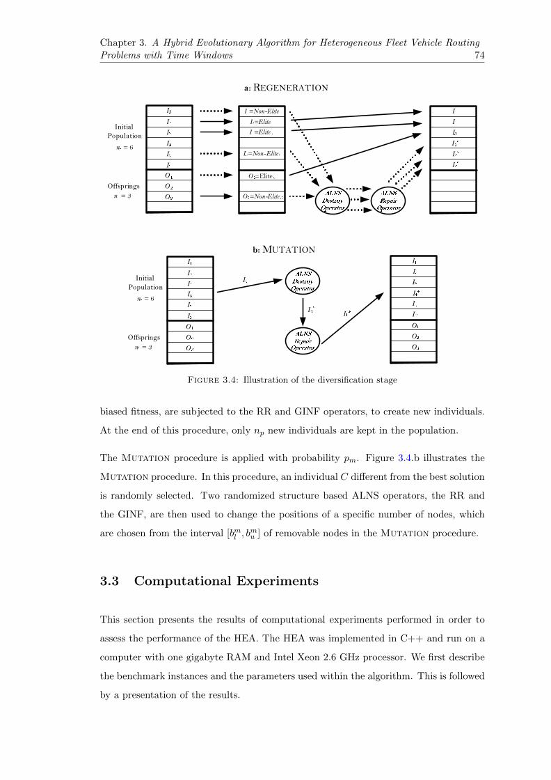
Chapter 3. A Hybrid Evolutionary Algorithm for Heterogeneous Fleet Vehicle RoutingProblems with Time Windows 74
Initial
Population
I1
Offsprings
I2
I3
I4
I5
I6
O1
O2
O3
np = 6
no = 3
I2=Elite1
I3
=Elite2
O1
=Elite3
I1
=Non-Elite1
I5
=Non-Elite2
O3
=Non-Elite3
I1
I2
I3
Initial
Population
I1
Offsprings
I2
I3
I4
I5
I6
O1
O2
O3
np = 6
no = 3
I1
I2
I3
I5
I6
a: REGENERATION
b:MUTATION
I4
I4
*
ALNS
Destroy
Operator
ALNS
Repair
Operator
ALNS
Destroy
Operator
ALNS
Repair
Operator
O1
O2
O3
I4
*
I4
*
I4
*
I5
*
I6
*
Figure 3.4: Illustration of the diversification stage
biased fitness, are subjected to the RR and GINF operators, to create new individuals.
At the end of this procedure, only np new individuals are kept in the population.
The Mutation procedure is applied with probability pm. Figure 3.4.b illustrates the
Mutation procedure. In this procedure, an individual C different from the best solution
is randomly selected. Two randomized structure based ALNS operators, the RR and
the GINF, are then used to change the positions of a specific number of nodes, which
are chosen from the interval [bml , bmu ] of removable nodes in the Mutation procedure.
3.3 Computational Experiments
This section presents the results of computational experiments performed in order to
assess the performance of the HEA. The HEA was implemented in C++ and run on a
computer with one gigabyte RAM and Intel Xeon 2.6 GHz processor. We first describe
the benchmark instances and the parameters used within the algorithm. This is followed
by a presentation of the results.

Chapter 3. A Hybrid Evolutionary Algorithm for Heterogeneous Fleet Vehicle RoutingProblems with Time Windows 75
3.3.1 Data sets and experimental settings
The benchmark data sets of Liu and Shen (1999b), derived from the classical Solomon
(1987) VRPTW instances with 100 nodes, are used as the test-bed. These sets include
56 instances, split into a random data set R, a clustered data set C and a semi-clustered
data set RC. Sets shown by R1, C1 and RC1 have a short scheduling horizon and small
vehicle capacities, in contrast to sets denoted R2, C2 and RC2 with a long scheduling
horizon and large vehicle capacities. Liu and Shen (1999b) introduced three types of
cost structures, namely large, medium and small, and have denoted them by A, B
and C, respectively. The authors also introduced several vehicle types with different
capacities and fixed vehicle costs for each of the 56 instances. This results in a total of
168 benchmark instances for FT or FD.
The benchmark set used by Paraskevopoulos et al. (2008) for HT is a subset of the FT
instances, in which the fleet size is set equal to that found in the best known solutions
of Liu and Shen (1999a). In total, there are 24 benchmark instances derived from Liu
and Shen (1999a) for HT. We use the same set for HD, with the new objective.
Evolutionary algorithms use a set of correlated parameters and configuration decisions.
In our implementation, we initially used the parameters suggested by Vidal et al. (2012,
2013) for the genetic algorithm, but we have conducted several experiments to further
fine-tune these parameters on instances C101A, C203A, R101A, R211A, RC105A and
RC207A. Following these tests, the following parameter values were used in our exper-
iments: itt = 5000, itr = 2000, itw = 500, np = 25, no = 25, ne = 10, nc = 3, pm ∈
[0.4, 0.6], [bil, biu] = [0.3, 0.8], [bel , b
eu] = [0.1, 0.16], [bml , b
mu ] = [0.1, 0.16], σ1 = 3, σ2 =
1, σ3 = 0. For the Adaptive Large Neighborhood Search (ALNS), we have used the
same parameter values as in Demir et al. (2012), namely rp = 0.1, ϕ1 = 0.5, ϕ2 =
0.25, ϕ3 = 0.15, ϕ4 = 0.25. All of these settings are identical for all four considered
problems.
Table 3.1 presents the results of a fine-tuning experiment on parameters np and no, and
to test the effect of these parameters on the solution quality.
The table shows the percent gap between the solution value obtained by the HEA and the
best-known solution (BKS) value, averaged over the six chosen instances. The maximum

Chapter 3. A Hybrid Evolutionary Algorithm for Heterogeneous Fleet Vehicle RoutingProblems with Time Windows 76
Table 3.1: Average percentage deviations of the solution values found by the HEAfrom best-known solution values with varying np and no
nonp 10 25 50 75 100
10 0.42 0.26 0.38 0.56 0.6925 0.19 0.11 0.26 0.37 0.4950 0.39 0.29 0.30 0.45 0.5775 0.56 0.42 0.51 0.61 0.68100 0.67 0.53 0.61 0.72 0.78
population size is dependent on np and no, both of which have a significant impact on
the solution quality, where the best setting is obtained with np = no = 25.
Table B.3 in Appendix B presents the number of iterations as a percentage operators
by education operator. Table B.3 shows that over nine removal operators ACUTR
operator is used by 15.48% on average, which is the highest one. This results indicated
that ACUTR operator is able to improve solution quality, this is probably due to its
heterogeneous based structure.
3.3.2 Comparative analysis
We now present a comparative analysis of the results of the HEA with those reported in
the literature. In particular, we compare ourselves against LSa (Liu and Shen 1999a),
LSb (Liu and Shen 1999b), T-RR-TW (Dell’Amico et al. 2007), ReVNTS (Paraskevopou-
los et al. 2008), MDA (Braysy et al. 2008), BPDRT (Braysy et al. 2009), AMP (Repoussis
and Tarantilis 2010) and UHGS (Vidal et al. 2014). The comparisons are presented in
tables, where the columns show the total cost (TC), and percent deviations (Dev) of the
values of solutions found by each method with respect to the HEA. The first column
displays the instance sets and the number of instances in each set in parentheses. The
rows named Avg (%), Min (%) and Max (%) show the average, minimum and maximum
deviations across all benchmark instances, respectively. A negative deviation shows that
the solution found by the HEA is of better quality. In the column labeled BKS, “=”
shows the total number of matches and “<” shows the number of new BKS found for
each instance set.
Ten separate runs are performed for each instance, the best one of which is reported. For
each instance, a boldface refers to match with current BKS, where as a boldface with a

Chapter 3. A Hybrid Evolutionary Algorithm for Heterogeneous Fleet Vehicle RoutingProblems with Time Windows 77
“*” indicates new BKS. For detailed results, the reader is referred to Appendix B. Tables
B.1–B.9 present the fixed vehicle cost (VC), the distribution cost (transportation cost)
(DC), the computational time in minutes (Time) and the actual number of vehicles used
(Mix), where the letters A–E correspond to the vehicle types and the upper numbers
denote the number of each type of vehicle used. For example, (A2B1) indicates that two
vehicles of type A and one vehicle of type B are used in the solution.
Tables 3.2 and 3.3 summarize the average comparison results of the current state-of-the-
art solution methods for FT and FD, compared with the HEA. According to Tables 3.2
and 3.3, the HEA is highly competitive, with average deviations ranging from −6.78%
to 0.03% and a worst-case performance of 0.66% for FT. The average performance of our
HEA is better than that of all the competitors for FT, except for the algorithm of Vidal
et al. (2014) which is slightly better on average. However, the HEA found 17 new best
solution and outperforms this algorithm on to the second type of FT instances, which
are less tight in terms of vehicle capacity. As for FD, average cost reductions range from
−0.90% to −0.02% and the worst- case performance is 0.94%. The HEA outperforms
all other algorithms in the literature for FD, including the UHGS of Vidal et al. (2014).
Table 3.4 presents the comparison results for each HT instance against LSa and ReVNTS.
We note that LSa only solved FT and not HT, which was the basis for setting the
number of available vehicles in ReVNTS. The results show that the HEA outperforms
both methods and yields higher quality solutions within short computation times. On
average, the total cost reductions obtained were −12.68% and −0.34% compared to
LSa and ReVNTS, with minimum deviations of −29.47% and −2.01% and maximum
deviations of −1.26% and 0.35%, respectively. Finally, Table 3.5 shows the results
obtained on the newly introduced HD.
Looking at the results obtained on the HT instances, on average the HEA yields 1.23%
and 0.13% lower vehicle fixed costs than the LSa and ReVNTS, respectively. The HEA
decreases the distribution cost (en-route time based cost) by 42.19% and 1.03%, com-
pared with LSa and ReVNTS, respectively. These results indicate that the HEA is able
find better fleet mix composition and lower distribution costs than the other methods.
The results also show that when ReVNTS and HEA find the same fleet mix composition
on a given instance, the distribution costs are lower in the solution found by the HEA,
indicating that our algorithm is more effective in finding better routes.

Chapter 3. A Hybrid Evolutionary Algorithm for Heterogeneous Fleet Vehicle RoutingProblems with Time Windows 78
Table3.2:
Ave
rage
resu
lts
for
FT
Inst
ance
set
T-R
R-T
WR
eVN
TS
MD
AA
MP
UH
GS
HE
AB
KS
TC
Dev
TC
Dev
TC
Dev
TC
Dev
TC
Dev
TC
=<
R1A
(12)
4180.8
3−
1.51
412
8.48
−0.
2441
31.3
1−
0.31
4113
.89
0.12
4103.1
60.
3841
18.7
00
0R
1B
(12)
1927.5
7−
1.65
190
2.19
−0.
3118
98.8
8−
0.13
1896
.83
−0.
031891.6
30.
2518
96.3
50
1*
R1C
(12)
1615.4
4−
2.56
158
2.18
−0.
4515
79.1
7−
0.26
1578
.12
−0.
191574.3
20.
0515
75.0
91
0C
1A
(9)
7229.0
2−
1.20
714
3.35
0.00
7141
.15
0.03
7139
.96
0.05
7138.9
30.
0671
43.3
52
0C
1B
(9)
2384.7
7−
0.99
236
1.78
−0.
0223
65.4
9−
0.18
2359
.82
0.06
2359.6
30.
0723
61.2
92
1*
C1C
(9)
1629.7
0−
0.62
162
1.09
−0.
0916
21.8
3−
0.14
1618.9
10.
0416
19.1
80.
0016
19.1
86
0R
C1A
(8)
5117.9
6−
3.49
496
1.69
−0.
3349
48.5
3−
0.07
4948
.02
−0.
064915.1
00.
6149
45.1
40
0R
C1B
(8)
2163.5
1−
1.35
214
2.65
−0.
3721
29.6
00.
2421
36.7
3−
0.09
2129.0
40.
2721
34.7
40
2*
RC
1C
(8)
1784.5
1−
1.36
176
9.93
−0.
5317
58.2
90.
1317
62.3
4−
0.10
1752.1
90.
4817
60.5
90
0R
2A
(11)
3568.9
7−
9.06
330
4.57
−0.
9833
10.7
0−
1.17
3287
.80
−0.
473267.3
10.
1632
72.4
82
1*
R2B
(11)
1727.0
4−
17.4
0149
8.97
−1.
8814
95.3
7−
1.64
1487
.09
−1.
0814
80.3
0−
0.61
1471.2
7*
17*
R2C
(11)
1436.2
2−
15.3
0128
1.31
−2.
8412
57.6
5−
0.94
1260
.97
−1.
201237.7
90.
6612
45.9
70
0C
2A
(8)
6267.7
5−
9.07
575
9.02
−0.
2257
97.3
8−
0.89
5749
.98
−0.
0657
60.2
9−
0.24
5746.4
4*
40
C2B
(8)
1897.6
2−
8.53
175
4.07
−0.
3217
56.0
8−
0.43
1748
.99
−0.
0317
50.3
7−
0.11
1748.5
2*
21*
C2C
(8)
1276.2
9−
4.78
123
2.98
−1.
2212
23.8
6−
0.47
1224
.08
−0.
4912
21.1
7−
0.25
1218.1
2*
42*
RC
2A
(8)
4752.9
5−
8.24
440
6.28
−0.
3443
99.1
2−
0.18
4388
.88
0.05
4381.7
30.
2143
91.1
60
0R
C2B
(8)
2156.1
1−
15.4
0188
8.83
−1.
1318
99.2
0−
1.68
1874
.86
−0.
3818
77.8
4−
0.54
1867.8
0*
02*
RC
2C
(8)
1828.9
5−
19.5
0156
7.22
−2.
4315
62.1
9−
2.10
1541
.13
−0.
7215
45.2
9−
0.99
1530.0
8*
00
Min
(%)
−19
.50
−2.
84−
2.10
−1.
20−
0.99
Avg
(%)
−6.
78−
0.76
−0.
57−
0.25
0.03
Max
(%)
−0.
620.
000.
240.
120.
66A
ll24
17*
Ru
ns
11
31
1010
Pro
cess
or
P60
0M
PIV
1.5G
Hz
Ath
2.6G
Hz
PIV
3.4G
Hz
Op
t2.
2GH
zX
e2.
6GH
zA
vg
Tim
e14
.15
20.
0010
.97
16.6
75.
084.
83

Chapter 3. A Hybrid Evolutionary Algorithm for Heterogeneous Fleet Vehicle RoutingProblems with Time Windows 79
Table3.3:
Ave
rage
resu
lts
for
FD
Inst
an
cese
tM
DA
BP
DR
TU
HG
SH
EA
BK
ST
CD
evT
CD
evT
CD
evT
C=
<
R1A
(12)
4068
.59−
0.67
4060
.96−
0.48
4031.2
80.
2540
41.4
60
0R
1B
(12)
1854
.60−
0.82
−−
1841
.43
−0.
111839.3
9*
04*
R1C
(12)
1539
.48−
0.91
1539
.90−
0.93
1530
.25
−0.
301525.5
6*
08*
C1A
(9)
7085
.56−
0.03
7085
.91−
0.04
7082.9
80.
007082.9
89
0C
1B(9
)23
35.1
1−
0.09
−−
2332.8
90.
0023
32.9
09
0C
1C(9
)16
15.7
5−
0.02
1615
.40−
0.01
1615
.49
−0.
011615.3
8*
90
RC
1A(8
)49
44.4
8−
0.57
4935
.52−
0.38
4891.2
50.
5149
16.4
10
0R
C1B
(8)
2121
.62−
0.87
−−
2107
.08
−0.
182103.2
1*
07*
RC
1C(8
)17
41.7
8−
0.94
1749
.66−
1.40
1734
.36
−0.
511725.4
4*
26*
R2A
(11)
3193
.41−
1.36
3180
.59−
0.96
3151
.96
−0.
053150.2
9*
74*
R2B
(11)
1392
.92−
3.06
−−
1351
.905
−0.
021351.5
2*
42*
R2C
(11)
1149
.65−
2.06
1149
.11−
2.01
1128
.708
−0.
201126.4
2*
54*
C2A
(8)
5690
.87−
0.07
5689
.40−
0.04
5686.7
50.
005686.7
58
0C
2B(8
)16
98.5
1−
0.69
−−
1686.7
50.
001686.7
58
0C
2C(8
)11
86.0
3−
0.07
1185
.70−
0.04
1185.1
90.
001185.1
98
0R
C2A
(8)
4241
.33−
0.73
4231
.25−
0.49
4210.1
00.
004210.1
05
1*
RC
2B(8
)17
04.1
3−
1.04
−−
1686
.63
−0.
011686.4
7*
05*
RC
2C(8
)13
74.5
5−
1.11
1385
.32−
1.91
1358
.24
0.08
1359
.33
13*
Min
(%)
−4.
30−
7.74
−1.
49A
vg
(%)
−0.
90−
0.74
−0.
02M
ax(%
)0.
070.
100.
94A
ll75
44*
Ru
ns
31
1010
Pro
cess
or
Ath
2.6G
Du
o2.
4GO
pt
2.2G
Xe
2.6G
Avg
Tim
e3.
56−
4.72
4.56

Chapter 3. A Hybrid Evolutionary Algorithm for Heterogeneous Fleet Vehicle RoutingProblems with Time Windows 80
Table3.4:
Res
ult
sfo
rH
T
Inst
ance
set
LSa
ReV
NT
SH
EA
BK
SM
ixT
CD
evM
ixT
CD
evD
CV
CM
ixT
CT
ime
=<
R10
1AA
1B
11C
11D
150
61−
10.2
9B
10C
11D
14583.9
90.
1019
98.7
625
90
B10C
11D
145
88.7
65.4
90
0R
102A
A1B
4C
14D
250
13−
13.2
5B
3C
14D
244
20.
680.
1317
36.5
426
40
A1B
4C
13D
24376.5
4*
6.78
01*
R10
3AB
7C
15
4772
−13
.57
B6C
15
4195.0
50.
1616
21.7
125
80
B6C
15
4201
.71
7.4
50
0R
104A
B9C
14
4455
−10
.61
B8C
14
4065
.52
−0.
9414
87.6
925
40
B9C
13
4027.6
9*
6.14
01*
C10
1AA
1B
10
9272
−5.
02B
10
8828.9
30.
0082
8.93
8000
B10
8828.9
33.
671
0C
102A
A19
8433
−17
.89
A19
7137.7
90.
2114
53.1
357
00
A19
7153
.13
4.1
20
0C
103A
A19
8033
−12
.78
A19
7143.
88−
0.30
1422
.57
5700
A19
7122.5
7*
3.45
01*
C10
4AA
19
7384
−4.
25A
19
7104.
96−
0.30
1383
.74
5700
A19
7083.7
4*
3.13
01*
RC
101A
A7B
7C
756
87−
7.99
A4B
7C
752
79.
92−
0.26
1876
.36
3390
A4B
7C
75266.3
6*
5.73
01*
RC
102A
A5B
6C
856
49−
10.7
7A
4B
5C
851
49.
95−
0.99
1709
.55
3390
A4B
5C
85099.5
5*
5.14
01*
RC
103A
A11B
2C
854
19−
8.58
A10B
2C
850
02.
41−
0.22
1691
.29
3300
A10B
2C
84991.2
9*
4.90
01*
RC
104A
A2B
13C
3D
151
89−
3.43
A2B
13C
3D
150
24.
25−
0.15
1596
.97
3420
A2B
13C
3D
15016.9
7*
5.21
01*
R20
1AA
545
93−
21.4
3A
53779.1
20.
0915
32.4
922
50
A5
3782
.49
7.4
50
0R
202A
A5
4331
−20
.85
A5
3578.9
10.
1413
33.9
222
50
A5
3583
.92
8.4
50
0R
203A
A4B
142
20−
18.7
4A
4B
135
82.
54−
0.8
110
53.9
225
00
A4B
13553.9
2*
7.12
01*
R20
4AA
538
49−
24.8
9A
531
43.
68−
2.01
831.
8022
50
A5
3081.8
0*
6.99
01*
C20
1AA
4B
167
11−
9.29
A4B
16140.6
40.
0074
0.64
5400
A4B
16140.6
44.
891
0C
202A
A1C
377
20−
1.26
A1C
377
52.
88−
1.69
623.
9670
00
A1C
37623.9
6*
4.26
01*
C20
3AC
2D
174
66−
2.23
C2D
17303.3
70.
0060
3.37
6700
C2D
17303.3
74.
371
0C
204A
A5
6744
−18
.72
A5
5721.
09−
0.72
680.
4650
00
A5
5680.4
6*
5.29
01*
RC
201A
C1E
358
71−
6.08
C1E
35523.1
50.
2116
84.5
938
50
C1E
355
34.5
96.4
70
0R
C20
2AA
1C
1D
1E
259
45−
15.4
3A
1C
1D
1E
25132.0
80.
3514
50.2
337
00
A1C
1D
1E
251
50.2
36.3
50
0R
C20
3AA
1B
1C
557
90−
29.4
7A
1B
1C
545
08.
27−
0.81
1221
.92
3250
A1B
1C
54471.9
2*
6.01
01*
RC
204A
A14B
249
83−
17.4
7A
14B
242
52.
87−
0.26
1441
.83
2800
A14B
24241.8
3*
5.87
01*
Min
(%)
−29
.47
−2.
01
Avg
(%)
−12
.68
−0.
34
Max
(%)
−1.
260.
35T
otal
314*
Runs
31
10P
roce
ssor
P23
3MP
IV1.
5GH
zX
e2.
6GH
zA
vg
Tim
e−
20.0
05.
61

Chapter 3. A Hybrid Evolutionary Algorithm for Heterogeneous Fleet Vehicle RoutingProblems with Time Windows 81
Table 3.5: Results for HD
Instance set HEADC VC Mix TC Time
R101A 1765.41 2590 B10C11D1 4355.41 5.19R102A 1716.44 2640 B4C13D2 4356.44 6.24R103A 1500.16 2580 B6C15 4080.16 6.57R104A 1434.72 2520 B7C14 3954.72 5.89C101A 828.94 8000 B10 8828.94 4.25C102A 1380.17 5700 A19 7080.17 3.97C103A 1379.21 5700 A19 7079.21 3.99C104A 1375.06 5700 A19 7075.06 2.98RC101A 1772.28 3390 A4B7C7 5162.28 6.41RC102A 1598.05 3420 A2B6C8 5018.05 5.24RC103A 1626.55 3300 A10B2C8 4926.55 4.39RC104A 1575.91 3420 A2B13C3D1 4995.91 4.88R201A 1198.76 2250 A5 3448.76 6.74R202A 1058.16 2250 A5 3308.16 8.13R203A 882.39 2500 A4B1 3382.39 7.49R204A 768.14 2250 A5 3018.14 5.47C201A 682.38 5400 A4B1 6082.38 4.21C202A 618.62 7000 A1C3 7618.62 3.69C203A 603.37 6700 C2D1 7303.37 3.67C204A 677.66 5000 A5 5677.66 5.11RC201A 1494.47 3850 C1E3 5344.47 6.72RC202A 1156.02 3700 A1C1D1E2 4856.02 6.48RC203A 996.25 3250 A1B1C5 4246.25 6.93RC204A 1395.32 2800 A14B2 4195.32 6.17Average 5224.77 5.45
Runs 10Processor Xe 2.6GHzAvg Time 5.45
In summary, the HEA was able to find 41 BKS for 168 FT instances, where 17 are
strictly better than those obtained by competing heuristics. As for FD, the algorithm
has identified 119 BKS out of the 168 instances, 44 of which are strictly better than those
obtained by previous heuristics. The results are even more striking for HT, with 17 BKS
on the 24 instances, 14 of which are strictly better than those reported earlier. Overall,
the HEA improves 75 BKS and matches 102 BKS out of 360 benchmark instances.

Chapter 3. A Hybrid Evolutionary Algorithm for Heterogeneous Fleet Vehicle RoutingProblems with Time Windows 82
3.4 Conclusions
We have proposed a unified heuristic for four types of heterogeneous fleet vehicle routing
problems with time windows. The first two are the Fleet Size and Mix Vehicle Routing
Problem with Time Windows (F) and the Heterogeneous Fixed Fleet Vehicle Routing
Problem with Time Windows (H). Each of these two problems was solved under a time
and a distance objective, yielding the four variants FT, FD, HT and HD. We have de-
veloped a unified hybrid evolutionary algorithm (HEA) capable of solving all variants
without any modification. This heuristic combines state-of-the-art metaheuristic prin-
ciples such as heterogeneous adaptive large scale neighborhood search and population
search. We have integrated within our HEA an innovative Intensification strategy on
elite solutions and we have developed a new diversification scheme based on the Regen-
eration and the Mutation of solutions. We have also developed an advanced version
of the Split algorithm of Prins (2009) to determine the best fleet mix for a set of routes.
Finally, we have introduced the new variant HD. Extensive computational experiments
were carried out on benchmark instances. In the case of FT, our HEA clearly outper-
forms all previous algorithms except that of Vidal et al. (2014). It performs slightly
worse on average, but is superior on instances which are less tight in terms of vehicle
capacity. On the FD instances, our HEA outperforms the three existing algorithms.
Overall, the HEA has identified 160 new best solutions out of 336 on the F instances,
61 of which are strictly better than previously known solutions. On the HT instances,
our HEA outperforms the two existing algorithms and has identified 17 best known so-
lutions out of 24, 14 of which are strictly better than previously found solutions. The
HD instances are solved here for the first time. Overall, we have improved 75 solutions
out of 360 instances, and we have matched 102 others. All instances were solved within
a modest computational effort. Our algorithm is not only highly competitive, but it is
also flexible in that it can solve four problem classes with the same parameter settings.

Chapter 4
The Fleet Size and Mix
Location-Routing Problem with
Time Windows: Formulations and
a Heuristic Algorithm
83

Chapter 4. The Fleet Size and Mix Location-Routing Problem with Time Windows:Formulations and a Heuristic Algorithm 84
Abstract
This paper introduces the fleet size and mix location-routing problem with time windows
(FSMLRPTW) which extends the location-routing problem by considering a heteroge-
neous fleet and time windows. The main objective is to minimize the sum of vehicle
fixed cost, depot cost and routing cost. We present mixed integer programming formula-
tions, a family of valid inequalities and we develop a powerful hybrid evolutionary search
algorithm (HESA) to solve the problem. The HESA successfully combines several meta-
heuristics and offers a number of new advanced efficient procedures tailored to handle
heterogeneous fleet dimensioning and location decisions. We evaluate the strengths of
the proposed formulations with respect to their ability to find optimal solutions. We also
investigate the performance of the HESA. Extensive computational experiments on new
benchmark instances have shown that the HESA is highly effective on the FSMLRPTW.
Keywords. location-routing; heterogeneous fleet; time windows; mixed integer program-
ming; genetic algorithm
4.1 Introduction
The design of distribution networks is critical for most companies because it usually
requires a major capital outlay. Two major types of decisions intervene in this process,
namely determining the locations of depots, and designing vehicle routes supplying cus-
tomers from these depots. In the classical Facility Location Problem (FLP) (Balinski
1965), it is assumed that each customer is served individually through a direct shipment,
which makes sense when customer demands are close to the vehicle capacity. However,
there exist several situations where customer demands can be consolidated. In such con-
texts, the FLP and Vehicle Routing Problem (VRP) should be solved jointly. The idea
of combining location and routing decisions was put forward more than fifty years ago
(Von Boventer 1961) and has given rise to a rich research known as the Location-Routing
Problem (LRP) (see Laporte 1988, Min et al. 1998, Nagy and Salhi 2007, Prodhon and
Prins 2014, Albareda-Sambola 2015, Drexl and Schneider 2015, for reviews). Applica-
tions of the LRP arise in areas as diverse as food and drink distribution, parcel delivery
and telecommunication network design. Many algorithms, mostly heuristics, have been

Chapter 4. The Fleet Size and Mix Location-Routing Problem with Time Windows:Formulations and a Heuristic Algorithm 85
developed for the LRP and its variations over the past fifty years, including some pop-
ulation metaheuristics (Prins et al. 2006b, Duhamel et al. 2010), neighborhood-based
metaheuristics (Prins et al. 2006a, Duhamel et al. 2011), simulated annealing (Karaoglan
et al. 2012) and adaptive large neighborhood search (ALNS) algorithms (Hemmelmayr
et al. 2012).
According to Hoff et al. (2010), heterogeneous fleets are more common in real-world
distribution problems than homogeneous ones. The Fleet Size and Mix VRP with Time
Windows (FSMVRPTW), introduced by Liu and Shen (1999b), is an LRP with a sin-
gle depot, a heterogeneous fleet and time windows. Many heuristics have also been
developed for the FSMVRPTW (see Irnich et al. 2014), including a two-stage construc-
tion heuristic (Liu and Shen 1999b), a sequential construction heuristic (Dullaert et
al. 2002), a multi-start parallel regret construction heuristic (Dell’Amico et al. 2007),
a three-phase multi-restart deterministic annealing metaheuristic (Braysy et al. 2008),
a hybrid metaheuristic combining a threshold acceptance heuristic with a guided local
search (Braysy et al. 2009), an adaptive memory programming algorithm (Repoussis
and Tarantilis 2010), and a genetic algorithm using a unified component based solution
framework (Vidal et al. 2014). This problem and a number of its variations are reviewed
by Baldacci et al. (2008) and Baldacci et al. (2009).
To our knowledge, a number of studies indirectly consider heterogeneous fleets in an
LRP context but without taking time windows into account (Ambrosino et al. 2009,
Wu et al. 2010). Berger et al. (2007) only consider a distance constraint. Therefore,
combining heterogeneous fleets and time windows in the LRP is done here for the first
time. We believe there is methodological interest in solving the Fleet Size and Mix
Location-Routing Problem with Time Windows (FSMLRPTW).
In the FSMLRPTW, one considers a fleet of vehicles with various capacities and vehicle-
related costs, as well as a set of potential depots with opening costs and capacities, and a
set of customers with known demands and time windows. The FSMLRPTW consists of
opening a subset of depots, assigning customers to them and determining a set of routes
for heterogeneous vehicles such that all vehicles start and end their routes at their depot,
each customer is visited exactly once by a vehicle within a prespecified time window,
and the load of each vehicle does not exceed its capacity. The objective is to minimize
the total cost which is made up of three components: the depot operating cost, the fixed

Chapter 4. The Fleet Size and Mix Location-Routing Problem with Time Windows:Formulations and a Heuristic Algorithm 86
cost of the vehicles, and the total travel costs of the vehicles. It is assumed that these
costs are scaled over the same time horizon.
The contributions of this paper are as follows. We introduce the FSMLPRTW as a
new LRP variant. We develop a hybrid evolutionary search algorithm (HESA) with the
introduction of several algorithmic procedures specific to the FSMLRPTW. Namely, we
introduce the location-heterogeneous adaptive large neighborhood search (L-HALNS)
procedure equipped with a range of several new operators as the main Education
procedure within the search. We also propose an Initialization procedure to create
initial solutions, and a Partition procedure for offspring solutions. Finally, we develop
a new diversification scheme through the Mutation procedure of solutions.
The remainder of this paper is structured as follows. Section 4.2 formally defines the
problem and provides integer programming formulations together with valid inequalities.
Section 4.3 presents a detailed description of the HESA. Computational experiments are
provided in Section 4.4, and conclusions follow in Section 4.5.
4.2 Formulations for the Fleet Size and Mix Location-
Routing Problem with Time Windows
In this section, we first define the FSMLRPTW, and then present several integer pro-
gramming formulations and valid inequalities to strengthen them.
4.2.1 Notation and problem definition
The FSMLRPTW is defined on a complete directed graph G = (N ,A), where N =
N0∪Nc is a set of nodes in which N0 and Nc represent the potential depot and customer
nodes, respectively, and A = (i, j) : i ∈ N , j ∈ N\(i, j) : i ∈ N0, j ∈ N0, i 6= j is the
set of arcs. Each arc (i, j) ∈ A has a nonnegative distance cij . Here, the terms distance,
travel time and travel cost are used in interchangeably. Each customer i ∈ Nc has a
positive demand qi. A storage capacity Dk and a fixed opening cost gk are associated
with each potential depot k ∈ N0. The index set of vehicle types is denoted by H.
Let Qh and fh denote the capacity and fixed dispatch cost of a vehicle of type h ∈ H.
Furthermore, si corresponds to the service time of node i ∈ Nc, which must start within

Chapter 4. The Fleet Size and Mix Location-Routing Problem with Time Windows:Formulations and a Heuristic Algorithm 87
the hard time window [ai, bi]. If a vehicle arrives at customer i ∈ Nc before time ai, it
waits until ai to start servicing the customer.
To formulate the FSMLRPTW, we define the following decision variables. Let xhij be
equal to 1 if vehicle of type h travels directly from node i to node j and to 0 otherwise.
Let yk be equal to 1 if depot k is opened and to 0 otherwise. Let zik be equal to 1 if
customer i is assigned to depot k and to 0 otherwise. Let uhij be the total load of vehicle
of type h immediately after visiting node i and traveling directly to node j. Let fij be
the total load of the vehicle while traversing arc (i, j) ∈ A, which is the aggregation of
the uhij variables over H. Let thi be the time at which a vehicle of type h starts serving at
node i. Let ti be the time at which service starts at node i ∈ N , which is the aggregation
of the thi variables.
4.2.2 Integer programming formulations
The integer linear programming formulation of the problem, denoted by E1, is then:
(E1) Minimize∑k∈N0
gkyk +∑h∈H
∑k∈N0
∑i∈Nc
fhxhki +∑h∈H
∑(i,j)∈A
cijxhij (4.1)
subject to
∑h∈H
∑j∈N
xhij = 1 i ∈ Nc (4.2)
∑h∈H
∑j∈N
xhji =∑h∈H
∑j∈N
xhij i ∈ N (4.3)
∑h∈H
∑j∈N
uhji −∑h∈H
∑j∈N
uhij = qi i ∈ Nc (4.4)
uhij ≤ Qhxhij i ∈ N0, j ∈ N , i 6= j, h ∈ H (4.5)∑h∈H
∑j∈Nc
uhkj =∑j∈Nc
zjkqj k ∈ N0 (4.6)
∑h∈H
∑j∈Nc
uhjk = 0 k ∈ N0 (4.7)
uhij ≤ (Qh − qi)xhij i ∈ Nc, j ∈ N , h ∈ H (4.8)
uhij ≥ qjxhij i ∈ N , j ∈ Nc, h ∈ H (4.9)∑i∈Nc
qizik ≤ Dkyk k ∈ N0 (4.10)
∑k∈N0
zik = 1 i ∈ Nc (4.11)
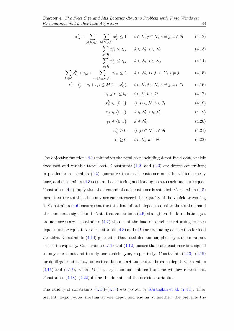
Chapter 4. The Fleet Size and Mix Location-Routing Problem with Time Windows:Formulations and a Heuristic Algorithm 88
xhij +∑
q∈H,q 6=h
∑l∈N ,j 6=l
xqjl ≤ 1 i ∈ N , j ∈ Nc, i 6= j, h ∈ H (4.12)
∑h∈H
xhik ≤ zik k ∈ N0, i ∈ Nc (4.13)∑h∈H
xhki ≤ zik k ∈ N0, i ∈ Nc (4.14)∑h∈H
xhij + zik +∑
m∈N0,m 6=kzjm ≤ 2 k ∈ N0, (i, j) ∈ Nc, i 6= j (4.15)
thi − thj + si + cij ≤M(1− xhij) i ∈ N , j ∈ Nc, i 6= j, h ∈ H (4.16)
ai ≤ thi ≤ bi i ∈ N , h ∈ H (4.17)
xhij ∈ 0, 1 (i, j) ∈ N , h ∈ H (4.18)
zik ∈ 0, 1 k ∈ N0, i ∈ Nc (4.19)
yk ∈ 0, 1 k ∈ N0 (4.20)
uhij ≥ 0 (i, j) ∈ N , h ∈ H (4.21)
thi ≥ 0 i ∈ Nc, h ∈ H. (4.22)
The objective function (4.1) minimizes the total cost including depot fixed cost, vehicle
fixed cost and variable travel cost. Constraints (4.2) and (4.3) are degree constraints;
in particular constraints (4.2) guarantee that each customer must be visited exactly
once, and constraints (4.3) ensure that entering and leaving arcs to each node are equal.
Constraints (4.4) imply that the demand of each customer is satisfied. Constraints (4.5)
mean that the total load on any arc cannot exceed the capacity of the vehicle traversing
it. Constraints (4.6) ensure that the total load of each depot is equal to the total demand
of customers assigned to it. Note that constraints (4.6) strengthen the formulation, yet
are not necessary. Constraints (4.7) state that the load on a vehicle returning to each
depot must be equal to zero. Contraints (4.8) and (4.9) are bounding constraints for load
variables. Constraints (4.10) guarantee that total demand supplied by a depot cannot
exceed its capacity. Constraints (4.11) and (4.12) ensure that each customer is assigned
to only one depot and to only one vehicle type, respectively. Constraints (4.13)–(4.15)
forbid illegal routes, i.e., routes that do not start and end at the same depot. Constraints
(4.16) and (4.17), where M is a large number, enforce the time window restrictions.
Constraints (4.18)–(4.22) define the domains of the decision variables.
The validity of constraints (4.13)–(4.15) was proven by Karaoglan et al. (2011). They
prevent illegal routes starting at one depot and ending at another, the prevents the

Chapter 4. The Fleet Size and Mix Location-Routing Problem with Time Windows:Formulations and a Heuristic Algorithm 89
creation of infeasible routes P = (vk1 , v1, v2, . . . , vs−1, vs, vl2) with s customers (k, l ∈
N0, k 6= l). Constraints (4.13) imply that zv1,k1 = 1. Since xv1,v2 = 1 and zv1,k1 = 1,
constraints (4.15) ensure that zv2,k1 = 1 and zv2,k2 cannot be equal to one.
Formulation E1 shown by (4.1)–(4.22) is valid for the FSMLRPTW. Other valid formu-
lations can be derived from E1. Before defining these formulations, we provide several
variations of E1 by aggregating some of the variables or disaggregating some of the
constraints. The reason is to either reduce the size of the formulation through aggre-
gation of variables or to tighten the linear relaxation bound by disaggregating some of
the constraints. First, fij which is the aggregation of the uhij variables, is obtained as
follows:
∑j∈N
fji −∑j∈N
fij = qi i ∈ Nc (4.23)
fij ≤∑h∈H
Qhxhij i ∈ N0, j ∈ N , i 6= j (4.24)∑j∈Nc
fkj =∑j∈Nc
zjkqj k ∈ N0 (4.25)
∑j∈Nc
fjk = 0 k ∈ N0 (4.26)
fij ≤∑h∈H
(Qh − qi)xhij i ∈ Nc, j ∈ N (4.27)
fij ≥ qj∑h∈H
xhij i ∈ N , j ∈ Nc. (4.28)
Let (f, x) be a solution satisfying constraints (4.23)–(4.28) and let (u, x) be a solution
satisfying constraints (4.2) and (4.4)–(4.9), where f, u and x are the respective vectors
for variables fij , uhij and xhij . Then, for each feasible (u, x), there exists a feasible (f, x)
and vice versa. Due to (4.2), there exists an h∗ ∈ H for which xh∗ij = 1 and due to (4.8),
there exists a uh∗ij ≥ 0, implying xhij = uhij = 0 for all other h ∈ H \ h∗. Using these
arguments, we have linked fij to the original variables in the following way:
fij =∑h∈H
uhij i, j ∈ N . (4.29)
We can now derive constraints (4.23)–(4.28) from (4.4)–(4.9) by using definition (4.29).
Constraints (4.23)–(4.28) are satisfied, since they are the same as (4.4)–(4.9), respec-
tively.
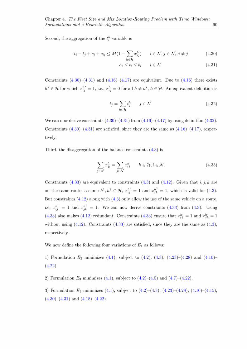
Chapter 4. The Fleet Size and Mix Location-Routing Problem with Time Windows:Formulations and a Heuristic Algorithm 90
Second, the aggregation of the thi variable is
ti − tj + si + cij ≤M(1−∑h∈H
xhij) i ∈ N , j ∈ Nc, i 6= j (4.30)
ai ≤ ti ≤ bi i ∈ N . (4.31)
Constraints (4.30)–(4.31) and (4.16)–(4.17) are equivalent. Due to (4.16) there exists
h∗ ∈ H for which xh∗ij = 1, i.e., xhij = 0 for all h 6= h∗, h ∈ H. An equivalent definition is
tj =∑h∈H
thj j ∈ N . (4.32)
We can now derive constraints (4.30)–(4.31) from (4.16)–(4.17) by using definition (4.32).
Constraints (4.30)–(4.31) are satisfied, since they are the same as (4.16)–(4.17), respec-
tively.
Third, the disaggregation of the balance constraints (4.3) is
∑j∈N
xhji =∑j∈N
xhij h ∈ H, i ∈ N . (4.33)
Constraints (4.33) are equivalent to constraints (4.3) and (4.12). Given that i, j, k are
on the same route, assume h1, h2 ∈ H, xh1
ij = 1 and xh2
jk = 1, which is valid for (4.3).
But constraints (4.12) along with (4.3) only allow the use of the same vehicle on a route,
i.e, xh1
ij = 1 and xh1
jk = 1. We can now derive constraints (4.33) from (4.3). Using
(4.33) also makes (4.12) redundant. Constraints (4.33) ensure that xh1
ij = 1 and xh1
jk = 1
without using (4.12). Constraints (4.33) are satisfied, since they are the same as (4.3),
respectively.
We now define the following four variations of E1 as follows:
1) Formulation E2 minimizes (4.1), subject to (4.2), (4.3), (4.23)–(4.28) and (4.10)–
(4.22).
2) Formulation E3 minimizes (4.1), subject to (4.2)–(4.5) and (4.7)–(4.22).
3) Formulation E4 minimizes (4.1), subject to (4.2)–(4.3), (4.23)–(4.28), (4.10)–(4.15),
(4.30)–(4.31) and (4.18)–(4.22).

Chapter 4. The Fleet Size and Mix Location-Routing Problem with Time Windows:Formulations and a Heuristic Algorithm 91
4) Formulation E5 minimizes (4.1), subject to constraints (4.2), (4.33), (4.23)–(4.28),
(4.10), (4.11), (4.13)–(4.15), (4.30)–(4.31) and (4.18)–(4.22).
4.2.3 Valid inequalities
We make use of four polynomial size valid inequalities which are proposed in the litera-
ture by several authors (Dantzig et al. 1954, Achuthan 2003, Labbe et al. 2004). These
were used by several authors for variants of LRPs (see Karaoglan et al. 2011, 2012). It
can be shown that these inequalities are also valid for the FSMLRPTW.
The first inequalities are special case of classical subtour elimination constraints for the
Traveling Salesman Problem (Dantzig et al. 1954) for two nodes as follows:
xhij + xhji ≤ 1 i, j ∈ Nc, h ∈ H. (4.34)
Constraints (4.34) break subtours involving two customers only. The second valid in-
equality, which was used by Labbe et al. (2004) for plant-cycle location problem is as
follows:
zik ≤ yk i ∈ Nc, k ∈ N0. (4.35)
Constraints (4.35) impose that customer i cannot be assigned to depot k if the latter
is not open. We now adapt the next valid inequality described by Achuthan (2003) for
the FSMLRPTW as follows:
∑h∈H
∑k∈N0
∑i∈Nc
xhki ≥ rα(Nc). (4.36)
Constraints (4.36) provide a lower bound on the number of routes originating from
depots where rα(Nc) =⌈∑
i∈Ncqi/max
h∈HQh⌉
and d•e is the smallest integer greater than
or equal to •. The fourth and final valid inequality is
∑k∈N0
yk ≥ ymin. (4.37)

Chapter 4. The Fleet Size and Mix Location-Routing Problem with Time Windows:Formulations and a Heuristic Algorithm 92
Constraints (4.37) bound the number of opened depots from below, where ymin is taken
as the minimum number of k opened depots satisfying∑
k∈N0Dk ≥
∑i∈Nc
qi after the
depots have been sorted in non-decreasing order of their capacity.
4.3 Description of the Hybrid Evolutionary Search Algo-
rithm
This section describes the proposed Hybrid Evolutionary Search Algorithm, called HESA,
that has been developed to solve the FSMLRPTW. This algorithm builds on several pow-
erful evolutionary based metaheuristic algorithms (see Koc et al. 2014, 2015, Vidal et
al. 2014). In this paper, we additionaly introduce the location-heterogeneous adaptive
large neighborhood search (L-HALNS) procedure which is used as a main Education
component in the HESA. Furthermore, we develope an Initialization to create initial
solutions and a Partition procedure to split offspring solutions into routes. Finally, we
propose a new Mutation procedure to diversify the solutions.
The general structure of the HESA is sketched in Algorithm 1. The initial population
is generated by using the Initialization procedure (line 1). Two parents are selected
(line 3) through a binary tournament process, where a crossover operation creates a
new offspring C (line 4), which then undergoes the Partition procedure (line 5). The
Education procedure uses the L-HALNS operators to educate offspring C and inserts
it back into the population (line 6). The probabilities associated with the L-HALNS
operators used in the Education procedure are updated by an Adaptive Weight Ad-
justment Procedure (AWAP) (line 7). The Intensification procedure which is based
on the L-HALNS is run on elite solutions (line 8). As new offsprings are added, the
population size na which is limited by np+no, changes over the iterations. The constant
np denotes the size of the population initialized at the beginning of the algorithm and
the constant no is the maximum allowable number of offspring that can be inserted into
the population. If the population size na reaches np+no at any iteration, then a survivor
selection mechanism is applied (line 9). The Mutation procedure is applied to a ran-
domly selected individual from the population with probability pm (line 10). When the
number $ of iterations without improvement in the incumbent solution is reached, the

Chapter 4. The Fleet Size and Mix Location-Routing Problem with Time Windows:Formulations and a Heuristic Algorithm 93
HESA terminates (line 11). For further implementation details on the ALNS based edu-
cation, parent selection, crossover, AWAP, intensification and survivor selection sections
the reader is referred to Chapter 3.
Algorithm 1 The general framework of the HESA
1: Initialization: initialize a population with size np2: while number of iterations without improvement < $ do3: Parent selection: select parent solutions P1 and P2
4: Crossover : generate offspring C from P1 and P2
5: Partition: partition offspring C into routes6: Education: educate C with L-HALNS and insert into population7: AWAP: update probabilities of the L-HALNS operators8: Intensification: intensify on elite solutions with L-HALNS9: Survivor selection: if the population size na reaches np+no, then select survivors
10: Mutation: diversify a random solution with probability pm11: end while12: Return best feasible solution
In what follows, we detail the algorithmic features specifically designed for the FSML-
RPTW. Section 4.3.1 presents the Initialization procedure of the population. The
Partition procedure is described in Section 4.3.2. Section 4.3.3 presents the offspring
Education procedure. Finally, the Mutation procedure is desribed in Section 4.3.4.
4.3.1 Initialization
We use a three-phase Initialization procedure to generate an initial population. The
first and second phases generate the initial solution while the third phase creates other
solutions. In the first phase, customers are assigned to the depots. Initially, the closest
depot according to its distance is calculated for each customer, and the customers are
listed in non-increasing order of distance. Each customer is then assigned to its closest
depot starting from the top of the list, without violating the depot capacities. These
steps are applied repeatedly to the residual customers who could not be assigned to
their closest depots due to depot capacity constraints. In this case they are assigned
to their closest feasible depot. In the second phase, routes are constructed for each
depot by applying the Clarke and Wright (1964) algorithm and by selecting the largest
vehicle type for each route. In the third phase, new individuals are created by applying
the L-HALNS operators to the initial solution until the initial population size reaches
np. A removal operator is randomly selected from a list of diversification based removal
operators and a greedy insertion with a noise function operator is used as an insertion

Chapter 4. The Fleet Size and Mix Location-Routing Problem with Time Windows:Formulations and a Heuristic Algorithm 94
operator (see Section 4.3.3). Both of these operators are used in order to diversify
the initial population. The number of nodes removed is randomly chosen from the
initialization interval [bil, biu] in the destroy phase. The interval is defined by a lower
and an upper bound calculated as a percentage of the total number of nodes in a given
instance.
4.3.2 Partition
We introduce a Partition procedure to be used in the L-HALNS (see Section 4.3.3).
The objective of this procedure is to split a given solution into routes after the parent
selection and the crossover phases during the algorithm. The given solution is repre-
sented as a permutation of customers. This procedure includes two phases. In the
first phase, the customer sequence is put into a list Lr. In the second phase, we use
an intensification-based insertion operator (greedy insertion operator) to insert the cus-
tomers of Lr to their best possible position. The Partition procedure yields a feasible
solution for the FSMLRPTW which is inserted into the population.
4.3.3 Education
At every iteration, the Education procedure is applied to the newly generated offspring
to improve its quality. The ALNS used as a way of educating the solutions, as in
Chapter 3, is basically an improvement heuristic. It consists of two procedures: removal,
followed by insertion. In the removal procedure, n′ nodes are iteratively removed by the
intensification based removal operators and placed in the removal list Lr, where n′ is in
the interval [bel , beu] for the destroy operators. In the insertion procedure, the nodes of
Lr are iteratively inserted into a least-cost position in the incomplete solution.
Here, we introduce the Location-HALNS (L-HALNS) which integrates fleet sizing and
the location decisions within the removal and insertion operators. This procedure dif-
fers from the Heterogeneous ALNS (HALNS) developed by Chapter 5 to educate the
solutions in the context of a heterogeneous fleet because the latter did not account for
the location decisions. When a node is removed, we check whether the resulting route
can be served by a smaller vehicle, and we also check whether the related depot has any
customer already assigned to it. We then update the solution accordingly. If inserting

Chapter 4. The Fleet Size and Mix Location-Routing Problem with Time Windows:Formulations and a Heuristic Algorithm 95
a node requires additional vehicle capacity or requires opening a new depot, we then
consider the option of using larger vehicles or the option of opening the least cost de-
pot not yet open. More formally, for each node i ∈ N0\Lr, let fh be the vehicle fixed
cost and let gk be the depot cost associated with this node. Let ∆(i) be the distance
saving obtained as a result of using a removal operator on node i. Let gk∗r be the depot
fixed cost and let fh∗r be the vehicle fixed cost after the removal of node i, i.e., gk∗r is
modified only if node i is the only node of depot k and fh∗r is modified only if the route
containing node i can be served by a smaller vehicle when removing node i. The savings
in depot fixed cost and vehicle fixed cost can be expressed as gk − gk∗r and fh − fh∗r ,
respectively. Thus, for each removal operator, the total savings resulting from removing
node i ∈ N0\Lr, denoted RC(i), is calculated as follows:
RC(i) = ∆(i) + (gk − gk∗r ) + (fh − fh∗r ). (4.38)
In the destroyed solution, the insertion cost of node j ∈ Lr after node i is defined as
Ω(i, j) on a given node i ∈ N0\Lr. Let gk∗a be the depot fixed cost and let fh∗a be the
vehicle fixed cost after the insertion of node i, i.e., gk∗r is modified only if node i requires
to open a new depot, or fh∗r is modified only if the route containing node i necessitates
the use of a larger capacity vehicle after inserting node i. The cost differences in depot
fixed cost and vehicle fixed cost can be expressed as gk∗r − gk and fh∗a − fh, respectively.
Thus, the total insertion cost of node i ∈ N0\Lr is IC(i), for each insertion operator is
IC(i) = Ω(i, j) + (gk∗r − gk) + (fh∗a − fh). (4.39)
Figure 4.1 provides an example of the removal and insertion phases of the L-HALNS
procedure.
4.3.3.1 Diversification based removal operators
The first and second diversification based removal operators were applied by Hemmel-
mayr et al. (2012), and the third one was used by Ropke and Pisinger (2006a). We
introduce the fourth one as a new operator specific to the FSMLRPTW.

Chapter 4. The Fleet Size and Mix Location-Routing Problem with Time Windows:Formulations and a Heuristic Algorithm 96
a) Feasible solution
Depot 1
Depot 2
Depot 3
1
2
3
45
6
7
8
9
10
Light
Medium
MediumHeavy
Lr =
b) Destroyed solution
Depot 1
Depot 2
Depot 3
1
2
3
45
6
7
8
9
10Medium
Heavy
Lr = 2,5,7,8,9
c) Repaired solution
Depot 1
Depot 2
Depot 3
1
2
3
45
6
7
8
9
10
Lr =
Heavy
Light
Medium
Medium
Figure 4.1: Illustration of the L-HALNS procedure
1. Depot closing removal (DR): This operator randomly selects an open depot and closes
it. The operator removes all customers of this depot. The DR operator also randomly
selects a closed depot and opens it.
2. Depot opening removal (DOR): The DOR operator randomly opens a closed depot.
The n′ customers removed from the solution are those which are closest to this depot
according to travel cost.
3. Random removal (RR): This operator randomly selects n′ customers and puts them
into the removal list.
4. Depot distance removal (DDR): The DSR operator is based on the DR operator but
differs from it by the criterion employed to open a closed depot. To open a depot, this
operator selects a closest depot with respect to a removed one.

Chapter 4. The Fleet Size and Mix Location-Routing Problem with Time Windows:Formulations and a Heuristic Algorithm 97
4.3.3.2 Intensification based removal operators
We now present the eight intensification based removal operators used in our algorithm.
The first seven were used in several papers (Ropke and Pisinger 2006a,b, Demir et al.
2012, Koc et al. 2015), whereas the last one is new.
1. Neighborhood removal (NR): The general idea behind the NR operator is to remove
n′ customers from routes that are extreme with respect to the average distance of a
route.
2. Worst distance removal (WDR): The WDR operator iteratively removes n′ high cost
customers, where the cost is based on the distance.
3. Worst time removal (WTR): This operator is a variant of the WDR operator. For
each node, costs are calculated, depending on the deviation between the arrival time and
the beginning of the time window. The WTR operator iteratively removes n′ customer
from the solution which has the largest deviation.
4. Shaw removal (SR): The SR operator aims to remove a set of n′ similar customers.
The similarity between two customers is based on distance, time, proximity and de-
mands.
5. Proximity-based removal (PBR): This operator is a special case of SR which is solely
based on distance.
6. Time-based removal (TBR): The TBR operator is another variant of SR. The selection
criterion of a set of customers is solely based on time.
7. Demand based-removal (DBR): The DBR operator is yet another variant of SR which
is solely based on demand.
8. Depot closing removal (DCR): The aim of the DCR operator is to calculate the
utilization efficiency of each depot Φ(k) (k ∈ N0) and remove from solution the one with
the least Φ(k) value. Φ(k) is expressed as the ratio of the total demand of depot k over
the capacity of depot k:
Φ(k) =
∑i∈Nc
qizik
Dk. (4.40)
Chapter 4. The Fleet Size and Mix Location-Routing Problem with Time Windows:Formulations and a Heuristic Algorithm 98
4.3.3.3 Insertion operators
Two insertion operators (Ropke and Pisinger 2006a,b, Demir et al. 2012, Koc et al. 2015)
are used in the repair phase of the Education procedure.
1. Greedy insertion operator (GIO): This operator finds the best possible insertion
position for all nodes in Lr while the cost calculation is based on distance. The insertion
process is iteratively applied to all nodes in Lr.
2. Greedy insertion with noise function operator (GINFO): The GINFO operator is a
variant of the GIO operator that extends it by allowing a degree of freedom in selecting
the best possible insertion position for a node.
4.3.4 Mutation
We introduce a Mutation procedure to increase the population diversity over the it-
erations (e.g., Nagata et al. 2010). This procedure is applied with probability pm. An
individual C different from the elite individuals is randomly selected. A randomly se-
lected diversification based removal operator and the GINFO operator are then used in
order to diversify the selected individual C. These two operators are applied to change
the positions of a specific number of nodes, which are chosen from the interval [bml , bmu ]
of removable nodes.
4.4 Computational Experiments
In this section, we present the results of computational experiments performed in order
to assess the performance of the formulations and the HESA. All experiments were con-
ducted on a server with one gigabyte RAM and Intel Xeon 2.6 GHz processor. We used
CPLEX 12.5 with its default settings as the optimizer to solve the integer programming
formulations. The HESA was implemented in C++.
Section 4.4.1 describes the benchmark instances and the experimental settings. The aim
of the computational experiments is threefold: (i) to analyze the effect of the metaheuris-
tic components (Section 4.4.2), (ii) to evaluate the formulation in terms of solving the
FSMLRPTW to optimality on small-size instances (Section 4.4.3), and (iii) to compare

Chapter 4. The Fleet Size and Mix Location-Routing Problem with Time Windows:Formulations and a Heuristic Algorithm 99
and test the integer programming formulation which is integrated with valid inequalities
and the HESA on small-medium-and large-size instances (Section 4.4.4).
4.4.1 Benchmark instances
Benchmark data sets for the FSMLRPTW were generated by considering the data set
described by Liu and Shen (1999b) for the Fleet Size and Mix VRP with Time Windows
(FSMVRPTW) and derived from the classical Solomon (1987) VRP with Time Windows
instances with 100 nodes. These sets include 56 instances, split into a random data set
R, a clustered data set C and a semi-clustered data set RC. The sets R1, C1 and RC1
have a short scheduling horizon and small vehicle capacities, in contrast to the sets R2,
C2 and RC2 which have a longer scheduling horizon and larger vehicle capacities. Liu
and Shen (1999b) also introduced three cost structures, namely A, B and C, and several
vehicle types with different capacities and fixed vehicle costs for each of the 56 instances.
In our data sets, we have used the cost structure A and generated small-size (10-15-20-
25-30-customer) as well as medium and large-size (50-75-100-customer) instances. We
have selected the first customers of each data sets to generate the instances, i.e., the
first 10 customers, 15 customers, and so on, of each Liu and Shen instance.
We followed a procedure similar to that used for the LRP benchmark instances (see
Barreto 2004, Albareda-Sambola et al. 2005, Prodhon 2006, Karaoglan et al. 2012) to
generate our depot characteristics. To this end, new depots features were added to
each instance of Liu and Shen, as shown in Appendix A.1. The depot characteristics
were generated using discrete uniform distributions. The depot coordinates are in the
range [0, 100]2. For the sets C1, C2, R1, R2, RC1 and RC2, the depot costs are in the
range [38000, 50000], [90000, 120000], [17000, 25000], [85000, 100000], [17000, 26000] and
[85000, 100000], respectively. The intervals for depot capacities for each data set and
for small-, medium- and large-size instances are given in Table 4.1. However, these data
ensure the opening of at least two depots for each instance. The main idea behind this
decision is to prevent to open only one depot in the solutions. In the original Solomon
instances there is only one depot; we have used this depot’s time windows for other
depots as well, i.e., in each data set, time windows are same for all depots.
Evolutionary algorithms use a set of correlated parameters. All algorithmic parametric
values were set as in Chapter 3, where an extensive meta-calibration procedure was used
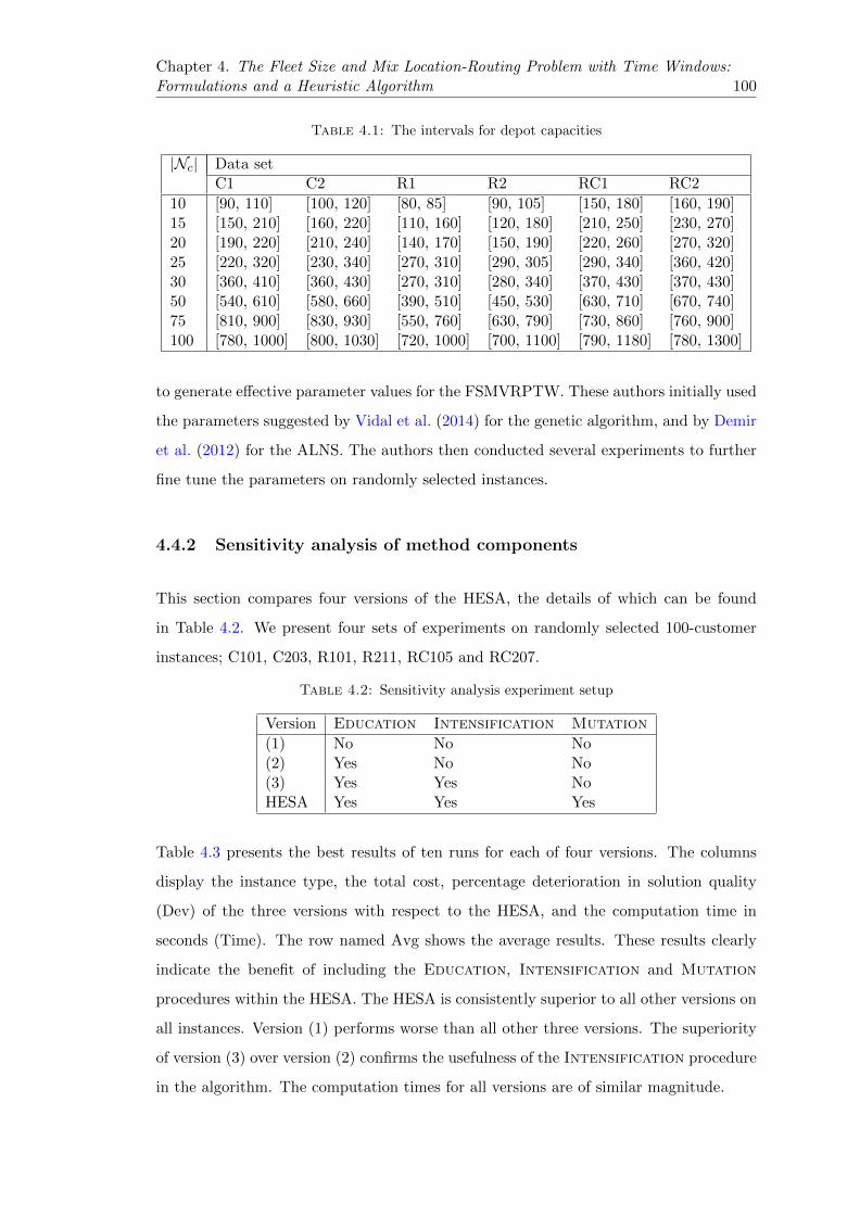
Chapter 4. The Fleet Size and Mix Location-Routing Problem with Time Windows:Formulations and a Heuristic Algorithm 100
Table 4.1: The intervals for depot capacities
|Nc| Data setC1 C2 R1 R2 RC1 RC2
10 [90, 110] [100, 120] [80, 85] [90, 105] [150, 180] [160, 190]15 [150, 210] [160, 220] [110, 160] [120, 180] [210, 250] [230, 270]20 [190, 220] [210, 240] [140, 170] [150, 190] [220, 260] [270, 320]25 [220, 320] [230, 340] [270, 310] [290, 305] [290, 340] [360, 420]30 [360, 410] [360, 430] [270, 310] [280, 340] [370, 430] [370, 430]50 [540, 610] [580, 660] [390, 510] [450, 530] [630, 710] [670, 740]75 [810, 900] [830, 930] [550, 760] [630, 790] [730, 860] [760, 900]100 [780, 1000] [800, 1030] [720, 1000] [700, 1100] [790, 1180] [780, 1300]
to generate effective parameter values for the FSMVRPTW. These authors initially used
the parameters suggested by Vidal et al. (2014) for the genetic algorithm, and by Demir
et al. (2012) for the ALNS. The authors then conducted several experiments to further
fine tune the parameters on randomly selected instances.
4.4.2 Sensitivity analysis of method components
This section compares four versions of the HESA, the details of which can be found
in Table 4.2. We present four sets of experiments on randomly selected 100-customer
instances; C101, C203, R101, R211, RC105 and RC207.
Table 4.2: Sensitivity analysis experiment setup
Version Education Intensification Mutation
(1) No No No(2) Yes No No(3) Yes Yes NoHESA Yes Yes Yes
Table 4.3 presents the best results of ten runs for each of four versions. The columns
display the instance type, the total cost, percentage deterioration in solution quality
(Dev) of the three versions with respect to the HESA, and the computation time in
seconds (Time). The row named Avg shows the average results. These results clearly
indicate the benefit of including the Education, Intensification and Mutation
procedures within the HESA. The HESA is consistently superior to all other versions on
all instances. Version (1) performs worse than all other three versions. The superiority
of version (3) over version (2) confirms the usefulness of the Intensification procedure
in the algorithm. The computation times for all versions are of similar magnitude.

Chapter 4. The Fleet Size and Mix Location-Routing Problem with Time Windows:Formulations and a Heuristic Algorithm 101
Table4.3:
Sen
siti
vit
yan
aly
sis
of
the
HE
SA
com
pon
ents
Inst
ance
Ver
sion
(1)
Ver
sion
(2)
Ver
sion
(3)
HE
SA
Tota
lco
stD
evT
ime
Tot
alco
stD
evT
ime
Tot
alco
stD
evT
ime
Tot
alco
stT
ime
C101
89091
.74
4.3
727
4.19
8709
1.74
2.17
279.
3486
590.
811.
6128
6.38
8519
9.09
297.
32C
203
19950
1.1
94.3
328
6.24
1968
01.7
13.
0229
4.13
1928
41.3
61.
0330
1.14
1908
64.0
030
8.09
R101
43941
.23
4.9
127
1.39
4284
1.17
2.47
276.
4142
640.
262.
0128
2.51
4178
2.20
292.
25R
211
18511
2.4
15.4
423
5.29
1801
19.7
32.
8124
0.13
1781
52.3
71.
7424
4.09
1750
51.0
024
7.03
RC
105
41640
.21
3.9
624
9.13
4134
0.21
3.27
271.
3140
840.
172.
0827
6.91
3999
0.10
281.
31R
C207
18307
1.9
14.2
628
0.17
1792
70.1
32.
2329
0.43
1782
74.3
61.
6829
4.37
1752
80.0
030
0.42
Avg
4.5
426
6.07
2.66
275.
291.
6928
0.90
287.
74

Chapter 4. The Fleet Size and Mix Location-Routing Problem with Time Windows:Formulations and a Heuristic Algorithm 102
4.4.3 Performance of the formulations
The formulations E1, E2, E3, E4 and E5 are examined in terms of their ability to solve
the FSMLRPTW to optimality on small-size (20-, 25-, and 30-customer) instances. To
analyze the computational results, we used the following performance measures: the
deviation (Dev) and computation time in seconds (Time) averaged over all instances for
each instance set (over a total of 840 experiments), and the number of optimal solutions
(#Op) obtained within one hour of computation time. Dev is the percentage deviation
between the Upper Bound (UB) and the best-known Lower Bound (LB), i.e., 100 (UB
− LB)/ UB. The upper bound is the optimal or best known solution obtained by solving
the formulations.
Table 4.4 presents comparative average results over the five formulations. The first
column displays the instance sets, and the following two columns show the number of
customers |Nc| and the number of depots |N0|, respectively. The overall results of E1 are
better than those of E3, thus we infer that constraints (4.6) strengthen formulation E1.
The results shown in Table 4.4 indicate that formulation E4 performs better than the
other models in terms of reaching optimal solutions within one hour of computation time.
These results imply that instead of constraints (4.4)–(4.9), using constraints (4.23)–
(4.28) which include the aggregated variables fij , and instead of constraints (4.16)–(4.17)
using constraints (4.30)–(4.31), which include the aggregated variables fij , yields better
formulations for the FSMLRPTW. Formulation E4 yields 27 optimal solutions out of 56
instances for the 20-customer instances, 13 out of 56 instances for 25-customer instances,
and nine out of 56 instances for 30-customer instances within the given time limit of one
hour. In terms of computation time, E4 provides on average lower computation time
than the other formulations.
We now investigate the effect of the valid inequalities on formulation E4. To this end,
we have conducted experiments on instances of the same size and we have used the same
performance measures as shown in Table 4.4. We used four variations of E4 denoted
as V1, V2, V3 and V4. Variation V1 is formulation E4 with valid inequalities (4.34), V2
is formulation E4 with valid inequalities (4.34) and (4.35), V3 is formulation E4 with
valid inequalities (4.34)–(4.36), and V4 is formulation E4 with valid inequalities (4.34)–
(4.37). Table 4.5 summarizes the average results of the effect of the valid inequalities
on formulation E4. These results show that V4, which includes all valid inequalities,

Chapter 4. The Fleet Size and Mix Location-Routing Problem with Time Windows:Formulations and a Heuristic Algorithm 103
Table4.4:
Ave
rage
resu
lts
of
the
form
ula
tion
s
Inst
ance
set|N
c||N
0|
E1
E2
E3
E4
E5
Dev
Tim
e#
Op
Dev
Tim
e#
Op
Dev
Tim
e#
Op
Dev
Tim
e#
Op
Dev
Tim
e#
Op
C1
(9)
205
0.07
2245
.17
40.
0719
78.4
25
0.08
2417
.07
50.
0825
05.7
44
0.08
2467
.02
3C
2(8
)20
50.
0722
45.1
77
0.00
844.
867
0.42
2782
.58
20.
0057
3.49
80.
0035
9.59
8R
1(1
2)20
50.
2929
47.2
63
0.28
2936
.22
30.
3230
19.0
32
0.21
3066
.77
30.
2030
19.3
12
R2
(11)
205
0.01
2059
.15
70.
0119
75.4
97
0.27
3291
.85
10.
0075
1.98
110.
0089
4.84
10R
C1
(8)
205
0.17
3228
.86
10.
1832
51.1
81
0.25
3208
.96
10.
1732
22.5
51
0.17
3192
.03
1R
C2
(8)
205
0.07
3600
.00
00.
0636
00.0
00
0.07
3600
.00
00.
0736
00.0
00
0.06
3600
.00
0A
vg
(Tot
al)
0.11
2720
.94
(22)
0.10
2431
.03
(23)
0.23
3053
.25
(11)
0.09
2286
.76
(27)
0.09
2255
.46
(24)
C1
(9)
255
0.12
2669
.77
30.
1124
80.2
33
0.16
3600
.00
00.
1432
07.5
71
0.14
3432
.45
1C
2(8
)25
50.
0216
07.9
15
0.05
1932
.03
50.
3131
51.2
81
0.00
1215
.17
60.
0011
20.6
26
R1
(12)
255
0.44
3302
.73
10.
4333
02.3
11
0.32
3151
.80
20.
3533
00.7
71
0.37
3301
.73
1R
2(1
1)25
50.
1733
25.5
11
0.11
3057
.42
20.
2433
08.4
81
0.03
2597
.39
40.
0629
57.5
92
RC
1(8
)25
50.
2236
00.0
00
0.22
3289
.92
10.
2333
05.7
41
0.20
3204
.17
10.
2133
67.1
11
RC
2(8
)25
50.
1036
00.0
00
0.07
3600
.00
00.
1036
00.0
00
0.09
3600
.00
00.
0736
00.0
00
Avg
(Tot
al)
0.18
3017
.65
(10)
0.16
2943
.65
(12)
0.23
3352
.88
(5)
0.14
2854
.18
(13)
0.14
2963
.25
(11)
C1
(9)
305
0.32
3600
.00
00.
2632
64.6
01
0.32
3600
.00
00.
3236
00.0
00
0.33
3600
.00
0C
2(8
)30
50.
0222
76.5
05
0.00
1478
.03
60.
2529
75.6
72
0.10
1545
.67
60.
1220
83.9
85
R1
(12)
305
0.48
3305
.80
10.
5033
17.9
61
0.72
3310
.17
10.
4933
03.8
11
0.47
3303
.81
1R
2(1
1)30
50.
2136
00.0
00
0.14
3434
.65
10.
3336
00.0
00
0.08
3159
.86
20.
0730
87.2
02
RC
1(8
)30
50.
3236
00.0
00
0.28
3600
.00
00.
3436
00.0
00
0.38
3600
.00
00.
3236
00.0
00
RC
2(8
)30
51.
2636
00.0
00
0.75
3600
.00
01.
0136
00.0
00
0.8
3600
.00
00.
6736
00.0
00
Avg
(Tot
al)
0.43
3330
.38
(6)
0.32
3115
.87
(9)
0.49
3447
.64
(3)
0.36
3134
.89
(9)
0.33
3212
.50
(8)

Chapter 4. The Fleet Size and Mix Location-Routing Problem with Time Windows:Formulations and a Heuristic Algorithm 104
Table4.5:
Eff
ect
of
the
vali
din
equ
ali
ties
Inst
ance
set|N
c||N
0|
V1
V2
V3
V4
Dev
Tim
e#
Op
Dev
Tim
e#
Op
Dev
Tim
e#
Op
Dev
Tim
e#
Op
C1
(9)
20
50.
0717
28.7
35
0.08
1694
.42
50.
0617
05.4
75
0.07
1881
.50
5C
2(8
)20
50.
0722
45.1
77
0.01
714.
347
0.01
628.
127
0.00
615.
458
R1
(12)
20
50.
2130
07.9
22
0.24
2757
.75
30.
2427
55.5
13
0.20
2613
.15
3R
2(1
1)
20
50.
0111
09.6
49
0.01
1141
.27
90.
0110
59.4
210
0.01
1029
.43
10R
C1
(8)
20
50.
1732
24.5
41
0.17
3208
.28
10.
1732
36.8
01
0.16
3199
.37
1R
C2
(8)
20
50.
0736
00.0
00
0.08
3600
.00
00.
0836
00.0
00
0.07
3600
.00
0A
vg
(Tota
l)0.
1024
86.0
024
0.10
2186
.01
250.
1021
64.2
226
0.09
2156
.48
27
C1
(9)
25
50.
1328
10.0
12
0.13
2795
.28
20.
1227
95.3
02
0.10
3193
.31
1C
2(8
)25
50.
0112
83.9
06
0.01
1369
.76
60.
0113
08.4
96
0.01
1126
.88
6R
1(1
2)
25
50.
3130
58.6
32
0.20
3143
.78
20.
2030
74.9
62
0.20
3075
.17
2R
2(2
2)
25
50.
0627
15.9
52
0.10
3561
.73
20.
2535
71.7
12
0.04
2839
.60
3R
C1
(8)
25
50.
2232
83.2
71
0.20
3289
.40
10.
1033
01.0
21
0.30
3258
.57
1R
C2
(8)
25
50.
1036
00.0
00
0.14
3600
.00
00.
1036
00.0
00
0.07
3600
.00
0A
vg
(Tota
l)0.
1427
91.9
613
0.13
2959
.99
130.
1329
41.9
113
0.12
2848
.92
13
C1
(9)
30
50.
2831
97.4
51
0.30
3591
.70
00.
3235
91.6
11
0.28
3249
.88
1C
2(8
)30
50.
1420
81.0
34
0.14
1822
.59
50.
1721
80.7
04
0.19
1930
.52
5R
1(1
2)
30
50.
4332
96.0
51
0.50
3295
.51
10.
4132
95.5
71
0.40
3295
.65
1R
2(2
2)
30
50.
1033
56.1
11
0.11
3434
.18
10.
0633
99.8
81
0.06
3321
.14
2R
C1
(8)
30
50.
2836
00.0
00
0.35
3600
.00
00.
3436
00.0
00
0.31
3600
.00
0R
C2
(8)
30
50.
8936
00.0
00
0.65
3600
.00
00.
7036
00.0
00
0.67
3600
.00
0A
vg
(Tota
l)0.
3531
88.4
47
0.34
3224
.00
70.
3332
77.9
67
0.32
3066
.20
9

Chapter 4. The Fleet Size and Mix Location-Routing Problem with Time Windows:Formulations and a Heuristic Algorithm 105
performs better than all other variations in terms of reaching optimal solutions within
one hour of computation time. For the 20-, 25-, and 30-customer instances, the solution
times are 2286.76, 2854.18 and 3134.89 seconds for E4, but these times are 2156.48,
2848.92, 3066.20 seconds for V4. Our results indicate that V4 yields same number of
optimal solutions as E4, but within smaller computation times.
4.4.4 Comparative analysis
We now present a comparative analysis of the results of the HESA and of the formulation
E4 integrated with valid inequalities, denoted by Ev4 . Each instance was solved once with
the HESA, and once with Ev4 . For Ev4 , a common time limit of three hours was imposed
on the solution time for all instances. For the HESA, ten separate runs are performed
for each instance, the best one of which is reported.
Tables 4.6 and 4.7 summarize the average results of the HESA compared with Ev4 . For
detailed results, the reader is referred to Appendix A. In Tables 4.6 and 4.7, the first
column displays the LP relaxation value of Ev4 , obtained by relaxing the integrality
constraints (4.18) on the Xhij variables only. Such a partial LP relaxation provides
better quality lower bounds compared to a full relaxation where the integer restrictions
(4.18)–(4.20) on all binary variables are relaxed, and in comparable solution times. The
remaining columns show the total time of all 10 runs of the HESA (Total time (s.)),
the time of the best solution (Time (s.)), the percent deviation values of the total cost
(DevTC) and of the vehicle cost (DevV C) found by Ev4 with respect to the HESA. In the
Time column, “*” denotes that the instance was not solved to optimality within three
hours.
Table 4.6 shows that the HESA finds almost the same solutions as those of Ev4 but in
a substantially smaller amount of time on the small-size FSMLPRTW instances. The
average time required by Ev4 to solve 10-, 15-, 20-, 25- and 30-customer instances to
optimality are 26.26, 3234.61, 6012.79, 8056.69 and 9359.53 seconds, respectively. For
the HESA, the respective statistics are 3.18, 3.95, 6.58, 8.93 and 13.05 seconds.
As can be observed from Table 4.7, the results clearly indicate that the HESA runs
quickly, also for medium and large-size instances. In particular, the algorithm requires
90.08, 167.82 and 299.98 seconds of average computation time to solve 50-, 75- and

Chapter 4. The Fleet Size and Mix Location-Routing Problem with Time Windows:Formulations and a Heuristic Algorithm 106
100-customer instances, respectively. The HESA is able to produce considerably better
results than Ev4 does in three hours. The improvements in solution values can be as
high as 6.42%, with an average of 1.41% for the 50-customer instances. Similarly, the
average improvement is 5.11% for the 75-customer instances, the highest value sitting
at 23.09%. The results are even more striking for the 100-customer instances where the
average total cost reduction obtained was 19.93% compared to Ev4 . In case of 50-, 75-
and 100-customer instances Ev4 was not able to find optimal solutions for 166 instances
out of 168 within three hours.
We now investigate the effect of the fleet mix composition on the FSMLRPTW instances
using the vehicle costs and DevV C values in Table 4.7. The results show that when opti-
mality is guaranteed by Ev4 , the HESA is able to find the optimal fleet mix composition.
For the 50- and 75-customer instances, the HESA decreased the vehicle costs by 8.08%
and 32.10% on average compared to Ev4 . This decrease ranges from 0.00 to 18.68% and
from 4.20% to 60.60% for the 50- and 75-customer instances, respectively. As for the
total costs, the results are even more striking for the 100-customer instances where the
average vehicle costs reduction obtained was 53.82% compared to Ev4 . These results im-
ply that for medium- and large-size instances, the HESA is able to produce substantially
lower vehicle costs than Ev4 .
4.5 Conclusions
This paper has introduced the FSMLRPTW, a complex integrated logistics problem
which, to our knowledge, was studied here for the first time, and has described a hybrid
evolutionary search algorithm tailored to the problem. We have introduced several al-
gorithmic procedures specific to the FSMLRPTW, namely, the location-heterogeneous
adaptive large neighborhood search procedure equipped with a range of new operators
as the main Education procedure within the search. We have also developed an Ini-
tialization procedure to create initial solutions, a Partition procedure for offspring
solutions, and a new diversification scheme through the Mutation procedure of solu-
tions. Computational results on a new set of benchmark instances of up to 100 nodes
and 10 potential depots were presented, which indicate that the proposed algorithm is
able to identify solutions within 0.05% of optimality for small size instances and yields

Chapter 4. The Fleet Size and Mix Location-Routing Problem with Time Windows:Formulations and a Heuristic Algorithm 107
Table4.6:
Ave
rage
resu
lts
on
small
-siz
ein
stan
ces
Inst
ance
set|N
c||N
0|
Ev 4
HE
SA
LP
rela
xat
ion
Veh
icle
cost
Tot
alco
stT
ime
(s.)
Veh
icle
cost
Tot
alco
stT
otal
tim
e(s
.)T
ime
(s.)
DevTC
DevVC
C1
(9)
103
8250
4.85
600.
0082
674.
640.
3860
0.00
8267
4.64
37.8
33.
570.0
00.0
0C
2(8
)10
319
1118
.19
755.
5619
2201
.84
2.07
755.
5619
2201
.84
34.4
53.
310.0
00.0
0R
1(1
2)10
339
382.
0491
1.11
3946
6.34
128.
6491
1.11
3946
6.34
31.0
23.
010.0
00.0
0R
2(1
1)10
317
5618
.55
1066
.67
1761
57.9
50.
9610
66.6
717
6157
.95
34.0
43.
180.0
00.0
0R
C1
(8)
103
3561
4.85
1222
.22
3571
6.90
10.7
712
22.2
235
716.
9034
.41
3.19
0.0
00.0
0R
C2
(8)
103
1734
34.9
813
77.7
817
3622
.24
14.7
613
77.7
817
3622
.24
30.7
52.
820.0
00.0
0A
vg
26.2
633
.75
3.18
0.00
0.0
0
C1
(9)
154
8188
9.59
900.
0082
059.
925.
5190
0.00
8205
9.92
45.8
34.
510.0
00.0
0C
2(8
)15
418
6126
.81
2000
.00
1871
93.6
39.
5220
00.0
018
7193
.63
37.8
83.
720.0
00.0
0R
1(1
2)15
439
590.
6436
0.00
3970
2.34
6328
.34
360.
0039
702.
4139
.27
3.86
0.0
00.0
0R
2(1
1)15
417
4662
.67
900.
0017
5190
.12
98.7
290
0.00
1751
90.1
239
.53
3.88
0.0
00.0
0R
C1
(8)
154
3584
3.17
660.
0035
961.
0534
69.0
766
0.00
3596
1.05
36.7
03.
600.0
00.0
0R
C2
(8)
154
1736
26.0
665
0.00
1738
26.2
194
96.5
165
0.00
1738
26.2
142
.24
4.15
0.0
00.0
0A
vg
3234
.61
40.2
43.
950.
000.0
0
C1
(9)
205
8223
6.26
1200
.00
8243
5.86
5263
.90
1200
.00
8245
0.45
63.5
26.
250.0
20.0
0C
2(8
)20
518
6141
.23
2000
.00
1872
24.0
660
1.82
2000
.00
1872
24.0
666
.28
6.46
0.0
00.0
0R
1(1
2)20
537
782.
9047
9.17
3813
9.76
8220
.94
479.
1738
139.
3763
.51
6.18
0.0
00.0
0R
2(1
1)20
517
4699
.40
900.
0017
5239
.55
1682
.87
900.
0017
5238
.39
64.9
26.
340.0
00.0
0R
C1
(8)
205
3607
5.96
870.
0036
242.
4595
07.2
087
0.00
3624
6.40
71.5
07.
040.0
10.0
0R
C2
(8)
205
1738
64.4
380
0.00
1740
79.4
510
800.
00*
800.
0017
4078
.67
74.0
17.
200.0
00.0
0A
vg
6012
.79
67.2
96.
580.
000.0
0
C1
(9)
255
8255
6.95
1500
.00
8276
7.35
8404
.21
1500
.00
8278
2.57
95.3
19.
330.0
20.0
0C
2(8
)25
518
6314
.82
2000
.00
1872
34.7
529
19.0
920
00.0
018
7234
.75
87.5
48.
450.0
00.0
0R
1(1
2)25
537
930.
6661
3.33
3830
6.32
9081
.98
613.
3338
287.
2294
.04
9.00
−0.
050.
00R
2(1
1)25
517
4795
.80
900.
0017
5313
.88
7563
.09
900.
0017
5311
.64
90.6
08.
960.0
00.0
0R
C1
(8)
255
3625
2.02
990.
0036
414.
3495
71.7
999
0.00
3643
0.18
95.2
69.
030.0
40.0
0R
C2
(8)
255
1740
75.9
610
00.0
017
4301
.53
1080
0.00
*10
00.0
017
4300
.67
91.1
88.
820.0
00.0
0A
vg
8056
.69
92.3
28.
930.
000.0
0
C1
(9)
305
8275
8.85
1800
.00
8309
6.43
9656
.17
1800
.00
8311
5.24
143.
4113
.84
0.0
20.0
0C
2(8
)30
518
6488
.20
2000
.00
1872
53.9
555
19.7
120
00.0
018
7252
.10
128.
6412
.56
0.0
00.0
0R
1(1
2)30
538
126.
3376
4.17
3854
3.11
9902
.81
764.
1738
495.
6711
9.46
11.7
5−
0.12
0.00
R2
(11)
305
1749
30.9
690
0.00
1753
71.6
094
78.5
090
0.00
1753
56.4
314
7.07
14.3
1−
0.01
0.00
RC
1(8
)30
536
474.
9611
32.5
036
715.
8010
800.
00*
1132
.50
3671
7.50
129.
8912
.69
0.0
00.0
0R
C2
(8)
305
3619
9.06
1131
.25
3655
5.58
1080
0.00
*11
31.2
536
572.
2313
2.83
13.1
80.0
50.0
0A
vg
9359
.53
133.
5513
.05
−0.
010.
00

Chapter 4. The Fleet Size and Mix Location-Routing Problem with Time Windows:Formulations and a Heuristic Algorithm 108
Table4.7:
Ave
rage
resu
lts
on
med
ium
-an
dla
rge-
size
inst
an
ces
Inst
ance
set|N
c||N
0|
Ev 4
HE
SA
LP
rela
xat
ion
Veh
icle
cost
Tot
al
cost
Tim
e(s
.)V
ehic
leco
stT
otal
cost
Tota
lti
me
(s.)
Tim
e(s
.)D
evTC
DevVC
C1
(9)
507
4138
6.56
2722
.22
4187
5.93
9644.
33272
2.22
4191
0.7
993
4.92
93.
090.
080.0
0C
2(8
)50
792
446.
1029
75.0
093
394.
7194
50.
78240
0.00
9282
2.4
599
6.13
99.
21−
0.6
1−
18.6
8R
1(1
2)50
738
870.
2213
50.0
039
722.
8710
800
.00*
130
1.67
3948
8.6
393
7.20
93.
32−
0.5
8−
3.4
2R
2(1
1)50
717
5518
.42
1540
.91
176
329
.57
1080
0.00
*135
0.00
1759
91.
7893
1.02
92.
70−
0.1
9−
9.9
0R
C1
(8)
507
1957
4.34
2081
.25
2280
7.06
10800
.00*
193
8.75
2048
5.7
476
9.46
76.
55−
6.4
2−
6.6
1R
C2
(8)
507
8706
5.42
2181
.25
8818
3.79
10800
.00*
186
8.75
8753
6.0
486
0.16
85.
62−
0.7
3−
9.8
7A
vg
10382
.52
904.8
290
.08
−1.4
1−
8.0
8
C1
(9)
758
8285
7.15
4511
.11
8366
2.53
10800
.00*
428
8.89
8347
9.5
017
39.4
9173
.35
−0.2
2−
4.2
0C
2(8
)75
818
8792
.53
7075
.00
192
980
.52
1080
0.00
*380
0.00
1893
74.
7516
62.9
1165
.39
−1.8
4−
37.4
6R
1(1
2)75
838
056.
2940
41.6
764
165.
0610
800
.00*
196
9.17
3993
9.2
617
26.1
4172
.11
−23.
09−
41.7
9R
2(1
1)75
817
4160
.82
5245
.45
178
597
.02
1080
0.00
*180
0.00
1746
01.
2716
21.9
8161
.90
−2.2
3−
60.6
0R
C1
(8)
758
3823
3.86
3086
.25
3952
3.52
10800
.00*
259
5.00
3876
8.8
917
41.3
9174
.04
−1.9
0−
14.6
4R
C2
(8)
758
1736
77.2
441
75.0
0176
872
.38
1080
0.00
*245
0.00
1743
67.
8816
08.3
9160
.14
−1.4
1−
33.8
9A
vg
10800
.00*
1683.
3816
7.82
−5.1
1−
32.1
0
C1
(9)
100
1084
345.
4570
44.4
486
863.
2910
800
.00*
578
8.89
8523
4.4
830
82.2
4307
.82
−1.8
3−
13.6
1C
2(8
)10
010
1900
77.5
422
887.
5033
0436
.31
10800
.00*
520
0.00
1908
62.
3830
83.7
9308
.28
−17.
58−
56.7
7R
1(1
2)10
010
3915
1.72
9831
.67
1662
96.2
610
800
.00*
264
8.33
4097
2.4
329
02.5
1289
.95
−65.
67−
66.6
9R
2(1
1)10
010
1747
94.1
112
068.
1818
5688
.94
10800
.00*
225
0.00
1751
71.
8229
34.8
0292
.88
−5.6
4−
80.0
1R
C1
(8)
100
1039
186.
4261
23.7
549
304.
2310
800
.00*
340
5.00
3988
9.1
830
62.5
4306
.05
−15.
53−
40.4
9R
C2
(8)
100
1017
4430
.65
1256
8.75
2687
49.9
210
800
.00*
296
2.50
1750
57.
7529
56.8
1294
.88
−13.
35−
65.3
5A
vg
10800
.00*
3003.
7829
9.98
−19.
93−
53.8
2

Chapter 4. The Fleet Size and Mix Location-Routing Problem with Time Windows:Formulations and a Heuristic Algorithm 109
better solutions for larger instances as compared to an off-the-shelf solver. The running
times of the algorithm are so that it can be used in practical applications.

Chapter 5
The Fleet Size and Mix
Pollution-Routing Problem
110

Chapter 5. The Fleet Size and Mix Pollution-Routing Problem 111
Abstract
This paper introduces the fleet size and mix pollution-routing problem which extends
the pollution-routing problem by considering a heterogeneous vehicle fleet. The main
objective is to minimize the sum of vehicle fixed costs and routing cost, where the latter
can be defined with respect to the cost of fuel and CO2 emissions, and driver cost.
Solving this problem poses several methodological challenges. To this end, we have
developed a powerful metaheuristic which was successfully applied to a large pool of
realistic benchmark instances. Several analyses were conducted to shed light on the
trade-offs between various performance indicators, including capacity utilization, fuel
and emissions and costs pertaining to vehicle acquisition, fuel consumption and drivers.
The analyses also quantify the benefits of using a heterogeneous fleet over a homogeneous
one.
Keywords. vehicle routing; fuel consumption; CO2 emissions; heterogeneous fleet; evo-
lutionary metaheuristic
5.1 Introduction
Road freight transport is a primary source of greenhouse gases (GHGs) emissions such
as carbon dioxide (CO2), the amount of which is directly proportional to fuel consump-
tion (Kirby et al. 2000). In the United Kingdom and in the United States, around a
quarter of GHGs comes from freight transportation (DfT 2012, EPA 2012). Greenhouse
gases mainly result from burning fossil fuel, and over 90% of the fuel used for freight
transportation is petroleum-based, which includes gasoline and diesel. These sources
account for over half of the emissions from the transportation sector (Kahn Ribeiro et
al. 2007).
Demir et al. (2011) have analyzed several models for fuel consumption and greenhouse
gas emissions in road freight transportation. Specifically, the authors have compared
six models and have assessed their respective strengths and weaknesses. These models
indicate that fuel consumption depends on a number of factors that can be grouped into
four categories: vehicle, driver, environment and traffic. The pollution-routing problem
(PRP), introduced by Bektas and Laporte (2011), is an extension of the classical vehicle

Chapter 5. The Fleet Size and Mix Pollution-Routing Problem 112
routing problem with time windows (VRPTW). It consists of routing vehicles to serve
a set of customers, and of determining their speed on each route segment to minimize
a function comprising fuel cost, emissions and driver costs. To estimate pollution, the
authors apply a simplified version of the emission and fuel consumption model proposed
by Barth et al. (2005), Scora and Barth (2006) and Barth and Boriboonsomsin (2009).
The simplified model assumes that in a vehicle trip all parameters will remain constant
on a given arc, but load and speed may change from one arc to another. As such, the
PRP model approximates the total amount of energy consumed on a given road segment,
which directly translates into fuel consumption and further into GHG emissions. Demir
et al. (2012) have developed an extended adaptive large neighbourhood search (ALNS)
heuristic for the PRP. This heuristic operates in two stages: the first stage is an extension
of the classical ALNS scheme to construct vehicle routes (Pisinger and Ropke 2007,
Ropke and Pisinger 2006a,b) and the second stage applies a speed optimization algorithm
(SOA) (Norstad et al. 2010, Hvattum et al. 2013) to compute the speed on each arc.
In a later study, Demir et al. (2014a) have introduced the bi-objective PRP which
jointly minimizes fuel consumption and driving time. The authors have developed a
bi-objective adaptation of their ALNS-SOA heuristic and compared four a posteriori
methods, namely the weighting method, the weighting method with normalization, the
epsilon-constraint method and a new hybrid method, using a scalarization of the two
objective functions.
The trade-off between minimizing CO2 emissions and minimizing total travel times was
studied by Jabali et al. (2012b) in the context of the time-dependent vehicle routing prob-
lem. The planning horizon was partitioned into two phases: free flow traffic and conges-
tion. The authors solved the problem via a tabu search and proposed efficient bound-
ing procedures. Franceschetti et al. (2013) have later introduced the time-dependent
pollution-routing problem where a two-stage planning horizon was used, as in Jabali
et al. (2012b). Such a treatment has allowed for an explicit modeling of congestion in
addition to the PRP objectives. The authors developed an integer linear programming
formulation in which vehicle speeds are optimally selected from a set of discrete values.
Kopfer and Kopfer (2013) studied the emission minimization vehicle routing problem
while considering a heterogeneous fleet. These authors described a mathematical formu-
lation for the problem and computed the CO2 emissions based on the payload and on
the traveled distance. They presented results of computational experiments performed

Chapter 5. The Fleet Size and Mix Pollution-Routing Problem 113
on small size instances with up to 10 customers. Kopfer et al. (2014) have analyzed the
potential of reducing CO2 emissions achievable by using an unlimited heterogeneous fleet
of vehicles of different sizes. Kwon et al. (2013) have considered the heterogeneous fixed
fleet vehicle routing problem with the objective of minimizing carbon emissions. They
presented a mathematical model enabling them to perform a cost-benefit assessment of
the value of purchasing or selling carbon emission rights. CO2 emissions are calculated
by fuel consumption which is based on the traveled distance of the vehicles. An upper
limit for the amount of CO2 was considered in order to introduce more flexibility into
an environmentally constrained network. The authors developed tabu search algorithms
and suggested that the amount of carbon emission can be reduced without sacrificing
the cost because of the benefit obtained from carbon trading. For other relevant refer-
ences and a state-of-the-art coverage on green road freight transportation, the reader is
referred to the survey of Demir et al. (2014b).
In most real-world distribution problems, customer demands are met with heterogeneous
vehicle fleets (Hoff et al. 2010). Two major problems belonging to this category are the
fleet size and mix vehicle routing problem introduced by Golden et al. (1984), which
works with an unlimited heterogeneous fleet, and the heterogeneous fixed fleet vehicle
routing problem proposed by Taillard (1999), which works with a known fleet. These
two main problems are reviewed by Baldacci et al. (2008) and Baldacci et al. (2009). To
our knowledge, the fleet size and mix vehicle routing problem combining time windows
with the PRP objectives, has not yet been investigated. We believe there is merit in
analyzing and solving the fleet size and mix pollution-routing problem (FSMPRP), not
only to quantify the benefits of using a flexible fleet with respect to fuel, emissions and
the relevant costs, but also to overcome the necessary methodological challenges to solve
the problem.
The contributions of this paper are threefold. First, we introduce the FSMPRP as a
new PRP variant. The second contribution is to develop a new metaheuristic for the
FSMPRP. Our third contribution is to perform analyses in order to provide managerial
insights, using the FSMPRP model and several variants. These analyses shed light on
the trade-offs between various method components and performance measures, such as
distance, fuel and emissions, enroute time and vehicle types. They also highlight and
quantify the benefits of using a heterogeneous fleet of vehicles over a homogeneous fleet.

Chapter 5. The Fleet Size and Mix Pollution-Routing Problem 114
The remainder of this paper is structured as follows. Section 5.2 presents a background
on vehicle types and characteristics. Section 5.3 provides a formal description of the
FSMPRP and the mathematical formulation. Section 5.4 contains a detailed description
of the metaheuristic. Computational experiments and analyses are presented in Section
5.5, followed by conclusions in Section 5.6.
5.2 Background on Vehicle Types and Characteristics
Available studies on emission models (e.g., Demir et al. 2011, 2014b) show the significant
impact that the vehicle type has on fuel consumption. In a goods distribution context,
using smaller capacity vehicles is likely to increase the total distance travelled and may
also increase CO2 emissions. According to Campbell (1995a,b), if large vehicles are
replaced by a larger number of small vehicles, emissions are likely to increase, even
though a heavy duty vehicle which has a larger engine consumes more fuel per km than
a light duty vehicle. According to Kopfer et al. (2014), replacing a large vehicle by several
vehicles of different types may sometimes result in a reduction of CO2 emissions. Vehicle
type effects the engine friction factor, engine speed, engine displacement, aerodynamics
drag, frontal surface area and vehicle drive train efficiency; vehicle curb-weight and
payload, i.e., capacity, also play an important role in routing decisions.
In the United Kingdom, the Department of Environment, Food and Rural Affairs (DE-
FRA 2007) considers that higher-power engines do not necessarily result in fuel savings,
and although these types of engines usually have a larger residual value, they may not be
financially advantageous. The effects of curb weight and payload on fuel consumption
have been studied by some authors (Bektas and Laporte 2011, Demir et al. 2011). The
payload of the vehicle has an impact on inertia force, rolling resistance and road slope
force. Demir et al. (2011) point out that when compared with light and medium duty,
heavy duty vehicles consume significantly more fuel, primarily due to their weight. From
the perspective of payload reduction, a study by Caterpillar (2006) has shown that a
4.4% improvement in fuel savings can be reached through a 4500 kg reduction in payload
and in gross weight with respect to an initial weight of 36 tonnes. The corresponding
improvement is 8.8% for an initial weight of 27 tonnes. DEFRA (2012) states that a
17-tonne heavy duty vehicle emits 18% more CO2 per km when fully loaded, and 18%
less CO2 per km when empty, relative to emissions at half-load.

Chapter 5. The Fleet Size and Mix Pollution-Routing Problem 115
The curb weight and payload constitute the Gross Vehicle Weight Rating (GVWR)
of a vehicle. The United States Federal Highway Administration FHWA (2011) has
categorized vehicles into three main types according to the GVWR: light duty, medium
duty, and heavy duty. In practice, the prominent truck companies produce mainly three
vehicle types for distribution (MAN 2014a, Mercedes-Benz 2014, Renault 2014, Volvo
2014). In our study, we consider the three main vehicle types of MAN (2014a), shown in
Figure 5.1, particularly as the market share of the trucks of MAN (2014a) was around
16.3% in Western Europe in 2013 (Statista 2013). These three vehicle types, i.e., light
duty, medium duty and heavy duty, are called TGL, TGM and TGX by MAN (2014a).
TGL and TGM are Single-Unit Trucks and TGX is a Single-Trailer Truck (FHWA 2011).
A list of and values for the common parameters (Demir et al. 2012, 2014a, Franceschetti
et al. 2013) for all vehicle types and specific parameters (MAN 2014a,b,c) for each vehicle
type are given in Tables 5.1 and 5.2, respectively. For further details on TGL, TGM
and TGX vehicles and their engines the reader is referred to MAN (2014a,b,c).
Table 5.1: Vehicle common parameters
Notation Description Typical values
ξ fuel-to-air mass ratio 1g gravitational constant (m/s2) 9.81ρ air density (kg/m3) 1.2041Cr coefficient of rolling resistance 0.01η efficiency parameter for diesel engines 0.45fc fuel and CO2 emissions cost (£/liter) 1.4fd driver wage (£/s) 0.0022κ heating value of a typical diesel fuel (kj/g) 44ψ conversion factor (g/s to L/s) 737ntf vehicle drive train efficiency 0.45vl lower speed limit (m/s) 5.5 (or 20 km/h)vu upper speed limit (m/s) 27.8 (or 100 km/h)θ road angle 0τ acceleration (m/s2) 0
Daily vehicle fixed costs fh are determined according to the United Kingdom Depart-
ment for Transport (DfT 2010). These costs combine the capital cost and the annual
fixed cost, which itself includes depreciation, repairs and maintenance, tires, insurance
and vehicle excise duty. In this paper, we assume that each vehicle route can be com-
pleted in one day, so that we can transform the capital and annual cost values into daily
costs.

Chapter 5. The Fleet Size and Mix Pollution-Routing Problem 116
a)
Lig
ht
duty
veh
icle
: TG
Lb
) M
ediu
m d
uty
veh
icle
: TG
Mc)
Hea
vy d
uty
veh
icle
: TG
X
Figure5.1:
Th
ree
veh
icle
typ
es(M
AN
2014a)
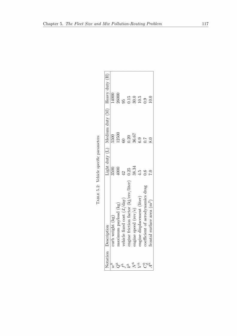
Chapter 5. The Fleet Size and Mix Pollution-Routing Problem 117
Table5.2:
Veh
icle
spec
ific
para
met
ers
Not
ati
on
Des
crip
tion
Lig
ht
du
ty(L
)M
ediu
md
uty
(M)
Hea
vy
du
ty(H
)
wh
curb
wei
ght
(kg)
3500
5500
1400
0Qh
maxim
um
pay
load
(kg)
4000
1250
026
000
fh
veh
icle
fixed
cost
(£/d
ay)
4260
95kh
engin
efr
icti
onfa
ctor
(kj/
rev/l
iter
)0.
250.
200.
15Nh
engin
esp
eed
(rev
/s)
38.3
436
.67
30.0
Vh
engi
ne
dis
pla
cem
ent
(lit
er)
4.5
6.9
10.5
Ch d
coeffi
cien
tof
aero
dynam
ics
dra
g0.
60.
70.
9Ah
fron
tal
surf
ace
area
(m2)
7.0
8.0
10.0

Chapter 5. The Fleet Size and Mix Pollution-Routing Problem 118
We use the comprehensive emissions model of Barth et al. (2005), Scora and Barth
(2006), and Barth and Boriboonsomsin (2008) to estimate fuel consumption and emis-
sions for a given time instant. This model has already been succesfully applied to the
PRP by Bektas and Laporte (2011), Demir et al. (2012, 2014a) and Franceschetti et al.
(2013). In what follows, we adapt the comprehensive emissions model to account for the
heterogeneous fleet case. The fuel consumption rate FRh (liter/s) of a vehicle of type h
is given by
FRh = ξ(khNhV h + P h/η)/κ, (5.1)
where the variable P h is the second-by-second engine power output (in kW) of vehicle
type h. It can be calculated as
P h = P htract/ntf + Pacc, (5.2)
where the engine power demand Pacc is associated with the running losses of the engine
and the operation of vehicle accessories such as air conditioning and electrical loads. We
assume that Pacc = 0. The total tractive power requirement P htract (in kW) for a vehicle
of type h is
P htract = (Mhτ +Mhg sin θ + 0.5Chd ρAv2 +MhgCr cos θ)v/1000, (5.3)
where Mh is the total vehicle weight (in kg) and v is the vehicle speed (m/s). The fuel
consumption F h (in liters) of vehicle type h over a distance d, is calculated as
F h = khNhV hλd/v + P hλγhd/v, (5.4)
where λ = ξ/κψ, γh = 1/1000ntfη and α = τ + g sin θ + gCr cos θ are constants. Let
βh = 0.5Chd ρAh be a vehicle-specific constant. Therefore, F h can be rewritten as
F h = λ(khNhV hd/v +Mhγhαd+ βhγhdv2). (5.5)
In this expression the first term khNhV hd/v is called the engine module, which is linear
in the travel time. The second term Mhγhαijd is referred to as the weight module,
and the third term βhγhdv2 is the speed module, which is quadratic in speed. These
functions will be used in the objective function of our model.
Chapter 5. The Fleet Size and Mix Pollution-Routing Problem 119
5.3 Mathematical Model for the Fleet Size and Mix Pollution-
Routing Problem
The FSMPRP is defined on a complete directed graph G = (N ,A) where N = 0, . . . , n
is the set of nodes, A = (i, j) : i, j ∈ N , i 6= j is the set of arcs, and node 0 corresponds
to the depot. The distance from i to j is denoted by dij . The customer set is Nc =
N\0, and each customer i has a positive demand qi. The index set of vehicle types
is denoted by H. If a vehicle arrives at customer i before ai, it waits until ai before
servicing the node. Furthermore, ti corresponds to the service time of node i ∈ N0,
which must start within time window [ai, bi].
The objective of the FSMPRP is to minimize a total cost function encompassing ve-
hicle, driver, fuel and emissions costs. A feasible solution contains a set of routes for
a heterogeneous fleet of vehicles that meet the demands of all customers within their
respective predefined time windows. Each customer is visited once by a single vehicle,
each vehicle must depart from and return to the depot, to serve a quantity of demand
that does not exceed its capacity. Furthermore, the speed of each vehicle on each arc
must be determined.
The binary variable xhij is equal to 1 if and only if a vehicle of type h ∈ H travels on
arc (i, j) ∈ A. The formulation works with a discretized speed function, proposed by
Bektas and Laporte (2011), defined by R non-decreasing speed levels vr (r = 1, . . . , R).
The binary variable zrhij is equal to 1 if and only if a vehicle of type h ∈ H travels on
arc (i, j) ∈ A at speed level r = 1, . . . , R, yj is the service start time at j ∈ Nc. The
total time spent on a route in which j ∈ Nc is the last visited node before returning to
the depot is defined by sj . Furthermore, let fhij be the amount of commodity flowing on
arc (i, j) ∈ A by a vehicle of type h. Therefore, the total load of vehicle of type h on
arc (i, j) is wh + fhij . We now present an integer linear programming formulation for the
FSMPRP:

Chapter 5. The Fleet Size and Mix Pollution-Routing Problem 120
(FSMPRP) Minimize∑h∈H
∑(i,j)∈A
λfckhNhV hdij
R∑r=1
zrhij /vr (5.6)
+∑h∈H
∑(i,j)∈A
λfcγhαijdij(w
hxhij + fhij) (5.7)
+∑h∈H
∑(i,j)∈A
λfcβhγhdij
R∑r=1
(vr)2zrhij (5.8)
+∑j∈Nc
fdsj +∑h∈H
∑j∈Nc
fhxh0j (5.9)
subject to
∑j∈Nc
xh0j ≤ mh ∀h ∈ H (5.10)
∑h∈H
∑j∈N
xhij = 1 ∀i ∈ Nc (5.11)
∑h∈H
∑i∈N
xhij = 1 ∀j ∈ Nc (5.12)∑h∈H
∑j∈N
fhji −∑h∈H
∑j∈N
fhij = qi ∀i ∈ Nc (5.13)
qjxhij ≤ fhij ≤ (Qh − qi)xhij ∀(i, j) ∈ A,∀h ∈ H (5.14)
yi − yj + ti +R∑r=1
dijzrhij /v
r ≤Mij(1− xhij) ∀i ∈ N , j ∈ Nc, i 6= j,∀h ∈ H (5.15)
ai ≤ yi ≤ bi ∀i ∈ Nc (5.16)
yj + tj − sj +
R∑r=1
dj0zrhj0 /v
r ≤ Lij(1− xhj0) ∀j ∈ Nc, ∀h ∈ H (5.17)
R∑r=1
zrhij = xhij ∀(i, j) ∈ A,∀h ∈ H (5.18)
xhij ∈ 0, 1 ∀(i, j) ∈ A,∀h ∈ H (5.19)
zrhij ∈ 0, 1 ∀(i, j) ∈ A, r = 1, . . . , R,∀h ∈ H(5.20)
fhij ≥ 0 ∀(i, j) ∈ A,∀h ∈ H (5.21)
yi ≥ 0 ∀i ∈ Nc. (5.22)
The first three terms of the objective function represent the cost of fuel consumption
and of CO2 emissions. In particular, term (5.6) computes the cost induced by the
engine module, term (5.7) reflects the cost induced by the weight module and term (5.8)

Chapter 5. The Fleet Size and Mix Pollution-Routing Problem 121
measures the cost induced by the speed module. Finally, term (5.9) computes the total
driver wage and the sum of all vehicle fixed costs.
The maximum number of vehicles available for each type is imposed by constraints (5.10).
We consider an unlimited number of vehicles for each vehicle type h (mh = |Nc|).
Constraints (5.11) and (5.12) ensure that each customer is visited exactly once. Con-
straints (5.13) and (5.14) define the flows. Constraints (5.15)–(5.17) are time window
constraints, where Mij = max0, bi + si + dij/vr − aj and Lij = max0, bj + tj +
maxidij/vr. Constraints (5.18) impose that only one speed level is selected for each
arc. Finally, constraints (5.19)–(5.22) enforce the integrality and nonnegativity restric-
tions on the variables.
5.4 Description of the Hybrid Evolutionary Algorithm
This section describes the proposed hybrid evolutionary algorithm, called HEA++, for
the FSMPRP. This algorithm builds on the HEA of Chapter 3, which is itself based on
the principles put forward by Vidal et al. (2014). In this paper, we have additionaly
developed the Heterogeneous Adaptive Large Neighborhood Search (HALNS) which is
used as a main Higher Education component in the HEA++. An adapted version of
the Speed Optimization Algorithm (SOA) (Norstad et al. 2010, Hvattum et al. 2013),
which works with a continuous speed variable, is applied on a solution within the al-
gorithm to optimize speeds between nodes. The combination of ALNS and SOA has
provided good results for the PRP (Demir et al. 2012, 2014a).
The general framework of the HEA++ is sketched in Algorithm 1. We now explain the
steps of the algorithm in reference to each line of Algorithm 1. The initial population is
generated by using a modified version of the classical Clarke and Wright (1964) savings
algorithm and the HALNS (line 1). A binary tournament process selects two parents
from the population (line 3) and combines them into a new offspring C via crossover (line
4), which then undergoes an improvement step through an advanced Split algorithm
with Speed Optimization Algorithm (Ssoa)(line 5). The Ssoa considers offspring C as
an input, in the form of a giant tour and then optimally splits it into vehicle routes. In
the Higher Education procedure, the HALNS with the SOA (line 6) are applied to
offspring C. If C is infeasible, this procedure is iteratively applied until a modified version

Chapter 5. The Fleet Size and Mix Pollution-Routing Problem 122
of C is feasible, which is then inserted into the population. The probabilities associated
with the Higher Education procedure operators are updated by the adaptive weight
adjustment procedure (AWAP) (line 7). The Intensification procedure is based on the
HALNS and SOA (line 8), and is run on elite solutions. The population size na is limited
by np +no, where np is a constant denoting the size of the initial population and no is a
constant showing the maximum allowable number of offsprings that can be inserted into
the population. A survivor selection mechanism is applied (line 9) if the populations size
na reaches np+no at any iteration. Mutation (line 10) is applied to a randomly selected
individual from the population with probability pm at each iteration of the algorithm.
The entire population undergoes a Regeneration (line 11) procedure if there are no
improvements in the best known solution for a given number of consecutive iterations
υ. When the number $ of iterations without improvement in the incumbent solution
is reached, the HEA++ terminates (line 13). For further implementation details on the
initialization, parent selection, crossover, AWAP, survivor selection and diversification
sections the reader is referred to Chapter 3.
Algorithm 1 General framework of the HEA
1: Initialization: initialize a population with size np2: while number of iterations without improvement < $ do3: Parent selection: select parent solutions P1 and P2
4: Crossover : generate offspring C from P1 and P2
5: Ssoa: partition C into routes6: Higher Education: educate C with HALNS and SOA and insert into popu-
lation7: AWAP: update probabilities of the HALNS operators8: Intensification: intensify elite solution with HALNS and SOA9: Survivor selection: if the population size na reaches np+no, then select survivors
10: Mutation: diversify a random solution with probability pm11: if number of iterations without improvement = υ then12: Regeneration: diversify the population with Regeneration procedures
13: end while14: Return best feasible solution
In what follows we detail the algorithmic features specifically developed for the FSMPRP.
The expanded version of the SOA is presented in Section 5.4.1, Ssoa is desribed in
Section 5.4.2, and finally, the Higher Education and Intensification procedures
are detailed in Section 5.4.3.

Chapter 5. The Fleet Size and Mix Pollution-Routing Problem 123
5.4.1 Speed optimization algorithm
The SOA is a heuristic procedure which optimizes the speed on each segment of a given
route in order to minimize an objective function comprising fuel consumption costs and
driver wages. Demir et al. (2012) adapted the arguments of Norstad et al. (2010) and
Hvattum et al. (2013) to the PRP, which we describe here for the sake of completeness.
The SOA is defined on a feasible path (0, ..., n+1) of nodes all served by a single vehicle,
where 0 and n+ 1 are two copies of the depot. The speed vi−1, represents the variable
speed between nodes i− 1 and i, ei is the arrival time at node i and ei is the departure
time from node i. The detailed pseude-code of the SOA is shown in Algorithm 2. The
SOA starts with a feasible route with initial fixed speeds, it takes input parameters
start node s and end node e, D and T which are respectively the total distance and
total service time, and returns speed-optimized routes. Initially, the speed vi−1, for
each link is calculated by considering the total distance of the route and the total trip
duration without the total service time (lines 4–7 of Algorithm 2). The SOA runs in
two stages where the main difference between these stages is the optimal speed v∗i−1
calculation (line 8 of Algorithm 2). In the first stage, optimal speeds are calculated as
v∗ =
(khNhV h
2βhγh+
fd2βhλγhfc
)1/3
, (5.23)
which minimizes fuel consumption and driver wage. The first stage fixes the arrival time
to the depot and uses this value as an input to the second stage where optimal speeds
are calculated using
v∗ =
(khNhV h
2βhγh
)1/3
, (5.24)
which minimizes fuel consumption in the second stage. The speeds are updated (lines
9–12 of Algorithm 2) if the vehicle arrives before ai and departs before bi or if the vehicle
arrives before bi and departs after bi+ ti. If node i is the last customer before the depot,
the speeds are recalculated to arrive at node i at ai (lines 13–14 of Algorithm 2). If vi−1
is lower than vl, then it is increased to vl, or if it is greater than vu, then it is decreased
to vu (lines 15–18 of Algorithm 2). The optimal speed is then compared with vi−1, if
the optimal speed is greater, vi−1 is then increased to the optimal speed (lines 19–20 of
Algorithm 2). The new arrival and departure times at node i are then calculated (lines
21–23 of Algorithm 2). If the departure time is less than ai + ti or if the arrival time

Chapter 5. The Fleet Size and Mix Pollution-Routing Problem 124
is greater than bi, the violation is calculated; otherwise, it is set to zero (lines 24–27
of Algorithm 2). At each iteration, the SOA selects the arc with largest time window
violation and eliminates the violation.
Algorithm 2 Speed Optimization Algorithm (s, e)
1: Input: violation← 0, p← 0, D ←∑e−1
i=s di, T ←∑e
i=s ti2: Output: Speed optimized routes3: for i = s+ 1 to e do4: if es ≤ as then5: vi−1 ← D/(ee − as − T )6: else7: vi−1 ← D/(ee − es − T )
8: v∗i−1 ← Optimal speed by equation (5.23) or (5.24)9: if ei−1 + di−1/vi−1 < ai and ei ≥ ai + ti and i 6= n then
10: vi−1 ← di−1/(ai − ei−1)11: else if ei−1 + di−1/vi−1 < bi and ei ≥ bi + ti and i 6= n then12: vi−1 ← di−1/(bi − ei−1)13: if i = n and ei 6= ei then14: vi−1 ← di−1/(ai − ei−1)15: if vi−1 < vl then16: vi−1 ← vl
17: else if vi−1 > vu then18: vi−1 ← vu
19: if v∗i−1 > vi−1 then20: vi−1 ← v∗i−1
21: ei ← ei−1 + di−1/vi−122: if i 6= n+ 1 then23: ei = ei + ti
24: gi ← max 0, ei − bi, ai + ti − ei25: if gi > violation then26: violation← gi27: p← i
28: end for29: if violation > 0 and ep > bp then30: ep ← bp + tp31: Speed Optimization Algorithm (s, p)32: Speed Optimization Algorithm (p, e)
33: if violation > 0 and ep < ap + tp then34: ep ← ap + tp35: Speed Optimization Algorithm (s, p)36: Speed Optimization Algorithm (p, e)
Chapter 5. The Fleet Size and Mix Pollution-Routing Problem 125
5.4.2 The Split algorithm with the speed optimization algorithm
The Split algorithm for heterogeneous vehicle routing problems Prins (2009), takes a
giant tour as an input and optimally splits it into vehicle routes. The splitting proce-
dure is based on solving the corresponding shortest path problem. Many extensions of
the Split algorithm have been successfully applied in evolutionary based heuristics for
several routing problems (Prins 2009, Vidal et al. 2014, Koc et al. 2015). Chapter 3 have
developed an advanced Split algorithm for a heterogeneous fleet. This algorithm was
embedded in the HEA to segment a giant tour and to determine the optimal fleet mix
through a controlled exploration of infeasible solutions (Cordeau et al. 2001, Nagata et
al. 2010). Time windows and capacity violations are penalized through a term in the
objective function. Here we introduce a new algorithmic feature, the Split algorithm
with the speed optimization algorithm (Ssoa) in which we incorporate the SOA within
the procedure for computing the cost of each arc in the shortest path problem.
5.4.3 Higher Education and Intensification
The classical ALNS scheme is based on the idea of gradually improving a starting solution
by using both destroy and repair operators on a given fleet mix composition. The ALNS
in Koc et al. (2015) uses nine removal and three insertion operators, selected from those
employed by various authors (Ropke and Pisinger 2006a,b, Pisinger and Ropke 2007,
Demir et al. 2012, Paraskevopoulos et al. 2008).
The ALNS is essentially a node improvement procedure and therefore does not explicitly
account for the heterogenous fleet dimension. In this paper, we propose the HALNS
which integrates fleet sizing within the removal and the insertion operators. For the
destroy phase of the HALNS, if a node is removed, we check whether the total demand
of the resulting route whether can be served by a smaller vehicle and we update the
solution accordingly. For the repair phase of the HALNS, if inserting a node requires
additional vehicle capacity, i.e., if the current vehicle cannot satisfy the total customer
demand, then we consider the option of using larger vehicle. Figure 5.2 provides an
example of the removal and insertion phases of the HALNS procedure.

Chapter 5. The Fleet Size and Mix Pollution-Routing Problem 126
Depot
8
2
10
3
4
11
5
71
96
Depot
8
2
10
3
4
11
5
71
96
Depot
8
2
10
3
4
11
5
71
96
a)Feasible solution
b)Destroyed solution
c)Repaired solution
Lr=
Lr= 7,2,3
Lr=
Heavy
Heavy
Medium
Medium
Medium
Light
Medium
Heavy
Mix: M
1
H2
Mix: L
1
M2
Mix: M
2
H1
Medium
Figure5.2:
Illu
stra
tion
of
theHALNS
pro
ced
ure

Chapter 5. The Fleet Size and Mix Pollution-Routing Problem 127
We redefine seven removal operators for the destroy phase of the HALNS procedure:
worst distance, worst time, neighborhood, Shaw, proximity-based, time-based and demand-
based. Furthermore, we redefine three insertion operators for the repair phase: greedy
insertion, greedy insertion with noise function and greedy insertion with en-route time.
Each operator has its own specific cost calculation mechanism. Aside from the distance
calculations, we account for the difference in the fixed vehicle cost within each operator.
The removal operators iteratively remove nodes, add them to the removal list Lr, and
update the fleet mix composition. The latter operation checks whether a vehicle with
a smaller capacity can serve the route after the node removal. The insertion operators
iteratively find the least-cost insertion position for node in Lr, where the cost compu-
tation includes the potential use of larger vehicles due to increasing the total demand
of the route. Therefore, the insertion operators insert the nodes in their best position
while updating the fleet mix composition.
For each node i ∈ Nc\Lr, let fh be the current vehicle fixed cost associated with the
vehicle serving i. Let ∆(i) be the saving obtained as a result of using a removal operator
on node i, as defined in the ALNS. Let fh∗r be the vehicle fixed cost after removal of
node i, i.e., fh∗r is modified only if the route containing node i can be served by a
smaller vehicle when removing node i. The saving in vehicle fixed cost can be expressed
as fh − fh∗r . Thus, the total savings of removing node i ∈ Nc\Lr, denoted RC(i), is
calculated as follows for each removal operator:
RC(i) = ∆(i) + (fh − fh∗r ). (5.25)
Given a node i ∈ Nc\Lr in the destroyed solution, we define the insertion cost of node
j ∈ Lr after node i as Ω(i, j). Let fh∗a be the vehicle fixed cost after the insertion of
node i, i.e., fh∗a is modified only if the route containing node i necessitates the use of
a larger capacity vehicle after inserting node i. The cost difference in vehicle fixed cost
can be expressed as fh∗a − fh. Thus, the total insertion cost of node i ∈ Nc\Lr is IC(i),
for each insertion operator is
IC(i) = Ω(i, j) + (fh∗a − fh). (5.26)

Chapter 5. The Fleet Size and Mix Pollution-Routing Problem 128
Chapter 3 developed a two-phase Intensification procedure whose main idea is to
improve the quality of elite individuals through intensifying the search within promising
regions of the solutions space. Here we introduce an extended version of this procedure.
We apply the HALNS by applying well-performing operators on the elite solutions.
Furthermore, we apply the SOA on the intensified elite solutions.
5.5 Computational Experiments and Analyses
We now summarize the computational experiments performed in order to assess the
performance of the HEA++. This algorithm was implemented in C++ and run on a
computer with one gigabyte of RAM and an Intel Xeon 2.6 GHz processor.
We have used the PRP library of Demir et al. (2012) as the test bed. These instances
were derived from real geographical distances of United Kingdom cities and are available
at http://www.apollo.management.soton.ac.uk/prplib.htm. From this library, we
have selected the four largest sets containing 75, 100, 150 and 200 nodes. Each set
includes 20 instances, resulting in a total of 80 instances. These PRP instances are cou-
pled with the parameters listed in Tables 5.1 and 5.2 for the FSMPRP. All algorithmic
parametric values were set as in Chapter 3, where an extensive meta-calibration proce-
dure was applied to generate effective parameter values for the standard heterogeneous
fleet vehicle routing problem with time windows.
The aim of the computational experiments is fourfold: (i) to analyse the effect of the
metaheuristic components (Section 5.5.1), (ii) to test the efficiency of the algorithm for
the solution of the PRP and the FSMPRP (Section 5.5.2), (iii) to empirically calculate
the savings that could be achieved by using a comprehensive objective function instead
of separate objective functions (Section 5.5.3), and (iv) to quantify the benefits of using
a heterogeneous fleet over a homogeneous one (Section 5.5.4).
5.5.1 Sensitivity analysis on method components
This section compares four versions of the HEA++ the details of which can be found
in Table 5.3. A “No” for HALNS implies using the ALNS of Chapter 3. Similarly, a

Chapter 5. The Fleet Size and Mix Pollution-Routing Problem 129
“No” for Ssoa corresponds to using the Split algorithm without SOA. Using the four
versions, we present four sets of experiments on the 100-node instances.
Table 5.3: Sensitivity analysis experiment setup
Version HALNS Ssoa
(1) No No(2) No Yes(3) Yes NoHEA++ Yes Yes
Table 5.4 presents the best results of ten runs on the instances for each of the four
versions. The first column displays the instances. The other columns show for each
version of the algorithm, the total cost (TC) in £, percentage deterioration in solution
quality (Dev) with respect to the HEA++, and the total computational time in minutes
(Time). The rows named Avg, Min (%) and Max (%) show the average results, as
well as minimum and maximum percentage deviations across all benchmark instances,
respectively.
The results clearly indicate the benefits of including the Ssoa and HALNS within the
HEA++. The HEA++ algorithm is consistently superior to all other three versions on
all 20 instances. Version (1) which uses the classical ALNS and Split corresponds to
the HEA of Chapter 3, performs worse than all other three versions. The superiority of
version (3) over version (2) confirms the importance of the HALNS component in the
algorithm. The computation times for all versions are of similar magnitude.
5.5.2 Results on the PRP and on the FSMPRP
To assess the quality of the HEA++, we have compared our algorithm with that of Demir
et al. (2012), referred to as DBL12, by using a homogenous fleet of vehicles with the
corresponding vehicle parameters used in the PRP. In Tables 5.5 and 5.6, we present the
computational results on the PRP instances with 100 and 200 nodes, respectively. The
columns show the number of vehicles used in the solution (NV) and the total distance
(TD). Ten separate runs were performed for each instance as done by DBL12, the best
of which is reported. For each instance, a boldface entry with a “*” indicates a new
best-known solution.

Chapter 5. The Fleet Size and Mix Pollution-Routing Problem 130
Table5.4:
Sen
siti
vit
yan
aly
sis
of
the
HE
A+
+co
mp
on
ents
Inst
an
ceV
ersi
on
(1)
Ver
sion
(2)
Ver
sion
(3)
HE
A+
+T
CD
evT
ime
TC
Dev
Tim
eT
CD
evT
ime
TC
Tim
e
UK
100
01
1041
.82
1.41
5.96
1036
.13
0.87
5.28
1035
.10
0.77
5.47
1027
.10
5.47
UK
100
02
1013
.75
1.07
4.41
1012
.71
0.97
4.27
1007
.86
0.50
4.21
1002
.87
4.38
UK
100
03
948.
482.
994.
0294
2.04
2.33
4.21
925.
670.
604.
9192
0.11
4.65
UK
100
04
1001
.54
0.92
4.16
1002
.47
1.01
4.35
994.
980.
274.
4999
2.32
4.74
UK
100
05
955.
122.
473.
4794
4.74
1.40
3.64
939.
830.
883.
9593
1.56
4.21
UK
100
06
1053
.98
1.49
4.63
1046
.18
0.76
4.55
1041
.51
0.31
5.19
1038
.25
5.63
UK
100
07
923.
601.
105.
3992
1.22
0.85
5.41
915.
880.
275.
4791
3.39
5.19
UK
100
08
982.
333.
853.
7896
7.55
2.38
4.09
953.
080.
904.
1194
4.51
4.52
UK
100
09
933.
294.
534.
5990
9.09
1.99
4.19
898.
450.
834.
4989
1.02
4.69
UK
100
10
1008
.24
1.87
3.87
992.
980.
362.
7399
1.59
0.22
3.29
989.
384.
19U
K100
11
1054
.71
1.87
4.87
1047
.71
1.21
3.91
1046
.18
1.07
4.19
1034
.98
5.13
UK
100
12
910.
793.
384.
2690
6.53
2.93
4.27
906.
952.
984.
5287
9.96
4.62
UK
100
13
1023
.71
2.23
4.46
1021
.32
2.00
4.53
1014
.79
1.37
4.79
1000
.86
4.78
UK
100
14
1069
.87
1.63
4.69
1063
.78
1.06
4.61
1058
.20
0.54
4.83
1052
.47
5.02
UK
100
15
1106
.50
2.04
4.57
1091
.11
0.66
4.59
1087
.32
0.31
4.81
1083
.95
5.27
UK
100
16
933.
250.
954.
3592
8.36
0.42
4.34
929.
980.
604.
5592
4.42
4.73
UK
100
17
1076
.11
1.75
3.79
1072
.18
1.38
4.29
1066
.71
0.88
4.29
1057
.33
4.36
UK
100
18
956.
433.
524.
5693
5.66
1.37
4.19
924.
920.
234.
4992
2.81
5.01
UK
100
19
941.
581.
803.
6793
9.75
1.61
3.81
930.
600.
644.
9992
4.60
4.99
UK
100
20
1093
.54
3.27
3.43
1070
.82
1.22
3.84
1066
.49
0.82
4.27
1057
.78
4.18
Avg
1001
.43
2.21
4.38
992.
621.
344.
2698
6.81
0.75
4.57
979.
484.
79M
in(%
)0.
920.
360.
22M
ax(%
)4.
532.
932.
98

Chapter 5. The Fleet Size and Mix Pollution-Routing Problem 131
The results clearly show that HEA++ outperforms DBL12 on all PRP instances in
terms of solution quality. The average cost reduction is 1.60% for 100-node instances,
for which the minimum and maximum improvements are 0.32% and 2.33%, respectively.
For 200-node instances, the corresponding values are 1.72% (average), 0.04% (minimum)
and 3.88% (maximum). On average, the Demir et al. (2012) is faster on the 100-node
instances, however, this difference is less substantial on the 200-node instances.
Table 5.5: Computational results on the 100-node PRP instances
Instance DBL12 HEA++NV TD TC Time NV TD TC Dev Time
UK100 01 14 2914.40 1240.79 1.54 14 2795.08 1212.72* −2.31 4.37UK100 02 13 2690.40 1168.17 1.64 13 2660.65 1149.16* −1.65 4.67UK100 03 13 2531.80 1092.73 3.47 13 2487.25 1080.87* −1.10 5.29UK100 04 14 2438.50 1106.48 2.49 14 2374.23 1085.66* −1.92 5.13UK100 05 14 2328.50 1043.41 2.65 14 2256.48 1033.19* −0.99 4.93UK100 06 14 2782.40 1213.61 2.23 14 2733.05 1192.67* −1.76 4.83UK100 07 12 2463.90 1060.08 1.71 12 2412.54 1044.58* −1.48 4.51UK100 08 13 2597.40 1106.78 3.49 12 2524.80 1092.67* −1.29 5.67UK100 09 13 2219.20 1015.46 2.57 13 2204.89 992.36* −2.33 4.97UK100 10 12 2510.10 1076.56 3.32 12 2432.26 1063.05* −1.27 5.64UK100 11 15 2792.10 1210.25 1.79 14 2722.22 1200.53* −0.81 4.11UK100 12 12 2427.30 1053.02 3.44 12 2336.10 1030.17* −2.22 5.64UK100 13 13 2693.10 1154.83 1.47 13 2589.17 1132.02* −2.01 3.49UK100 14 14 2975.30 1264.50 1.53 14 2892.45 1241.31* −1.87 4.29UK100 15 15 3072.10 1315.50 1.85 15 3038.40 1311.36* −0.32 3.87UK100 16 12 2219.70 1005.03 4.25 12 2203.99 986.57* −1.87 5.97UK100 17 15 2960.40 1284.81 2.55 15 2860.97 1257.44* −2.18 4.19UK100 18 13 2525.20 1106.00 1.54 13 2506.71 1088.89* −1.57 4.21UK100 19 13 2332.60 1044.71 1.52 13 2288.50 1024.17* −2.01 4.19UK100 20 14 2957.80 1263.06 3.41 14 2915.17 1249.84* −1.06 5.17
Avg 13.4 2621.61 1141.29 2.42 13.3 2561.75 1123.46 −1.60 4.76Min (%) −2.33Max (%) −0.32Processor Xe 3.0 GHz Xe 2.6 GHzRuns 10 10
Table 5.7 presents the average results obtained by HEA++ on the 75, 100, 150 and
200-node FSMPRP instances. For each instance set, the columns display the average
fuel and CO2 emissions cost (FEC), driver cost (DC) and vehicle cost (VC). To evaluate
the environmental impact of the solutions, we also report the average amount of CO2
emissions (in kg) based on the assumption that one liter of gasoline contains 2.32 kg
of CO2 (Coe 2005). For detailed results, the reader is referred to Tables D.1–D.4 in
the Appendix C, where ten runs were performed for each instance and the best one is
reported. We observe that on average, over all benchmark instances, the vehicle fixed

Chapter 5. The Fleet Size and Mix Pollution-Routing Problem 132
Table 5.6: Computational results on the 200-node PRP instances
Instance DBL12 HEA++NV TD TC Time NV TD TC Dev Time
UK200 01 28 4609.60 2111.70 12.10 28 4545.77 2067.00* −2.16 14.20UK200 02 24 4444.40 1988.64 17.00 25 4332.62 1953.35* −1.81 15.80UK200 03 27 4439.90 2017.63 6.74 28 4365.82 1996.13* −1.08 10.40UK200 04 26 4191.90 1934.13 6.86 26 4151.74 1905.88* −1.48 9.47UK200 05 27 4861.90 2182.91 15.40 27 4848.28 2151.99* −1.44 16.80UK200 06 27 3980.40 1883.22 7.51 27 3980.03 1859.40* −1.28 11.50UK200 07 27 4415.30 2021.95 15.70 27 4276.06 1974.32* −2.41 17.90UK200 08 27 4664.40 2116.76 7.17 27 4592.54 2088.12* −1.37 9.17UK200 09 25 4031.10 1894.18 9.22 25 3932.44 1823.50* −3.88 11.70UK200 10 28 4921.80 2199.95 8.33 27 4847.08 2166.59* −1.54 9.78UK200 11 27 4099.50 1941.19 14.10 27 4126.44 1908.83* −1.70 16.30UK200 12 25 4808.50 2105.14 11.90 26 4786.39 2104.40* −0.04 12.80UK200 13 25 4760.30 2141.26 7.41 25 4734.21 2094.48* −2.23 9.37UK200 14 27 4369.90 2011.35 7.51 27 4369.86 1994.49* −0.85 10.30UK200 15 25 4723.90 2110.86 9.04 26 4642.58 2067.48* −2.10 11.40UK200 16 27 4545.90 2075.83 7.59 27 4497.75 2023.55* −2.58 9.71UK200 17 26 4972.80 2218.28 6.82 26 4915.18 2165.34* −2.44 8.97UK200 18 27 4370.30 2004.68 13.20 27 4406.10 2003.75* −0.05 14.00UK200 19 25 3995.40 1844.90 16.20 25 3946.49 1803.56* −2.29 17.50UK200 20 27 4805.40 2150.57 8.85 26 4727.98 2114.31* −1.71 11.30
Avg 26.35 4500.60 2047.76 10.40 26.45 4451.27 2013.32 −1.72 12.40Min (%) −3.88Max (%) −0.04Processor Xe 3.0 GHz Xe 2.6 GHzRuns 10 10
cost accounts for 38.8% of the total cost, whereas the driver cost represents 36.7% of
the total, and the fuel and emissions cost accounts for 24.5%.
Table 5.7: Average results on the FSMPRP instances
Instance TD CO2 FEC DC VC TC Time
75-node 1534.38 345.74 208.63 280.15 296.40 785.185 3.27100-node 1841.48 414.17 249.93 354.56 375.00 979.484 4.79150-node 2398.78 550.48 332.18 509.66 536.40 1378.24 7.03200-node 2857.08 659.39 397.91 642.11 678.30 1720.42 10.4
5.5.3 The effect of cost components
This section analyzes the implications of using different cost components on the per-
formance measures. To this end, we have conducted experiments using four different
objective functions, which are presented in the rows of Table 5.8. The experiments were
conducted on a 100-node FSMPRP instance, and the best results collected over ten runs
are reported for each of four performance measures which we will now define. In min

Chapter 5. The Fleet Size and Mix Pollution-Routing Problem 133
TD, we consider the objective of minimizing the total distance. In min FEC, we only
consider fuel and emissions cost. This setting also implies minimizing CO2 since this
is proportional to fuel consumption. In min DC, we account only for the driver cost.
The min TD+VC objective corresponds to the standard heterogeneous vehicle routing
problems, which consists of minimizing distance and vehicle fixed costs. Finally we
present the FSMPRP objective. Aside from the objective function values, we provide
the main cost components in Table 5.8. In Table 5.9, we report the deviations from
the smallest cost components shown in Table 5.8. For example, the minimum value for
the total distance objective (min TD) is 1921.66 km, but the FEC objective yields a
solution with a total distance of 2119.87 km, corresponding to an increase of 10.31%.
It is clear that considering only distance in the objective results in a poor total cost
performance, yielding a 4.11% increase. This increase is more substantial when looking
only at the vehicle fixed cost where min TD is 8.65% higher in terms of VC. With respect
to CO2 emissions, the closest objective value is min TD+VC. This result implies that
a substantial gain in CO2 emissions can be achieved by using the TD+VC objective.
However, minimizing CO2 emissions yields an average increase of 1.09% in TC. Similar
to the TD objective, the DC objective performs poorly on all cost components, yielding
an average increase of 20.67% in the CO2 emissions.
In order to quantify the added value of changing speeds, we have experimented with
three other versions of the FSMPRP in which the speed on all arcs is fixed at 70, 85
or 100 km/h. Table 5.10 presents the results of these experiments. The results suggest
that while optimizing speeds with HEA++ yields the best results, using a fixed speed of
100 km/h deteriorates the solution quality by only 1.16% on average. This makes sense
since high driver costs will make it economical to drive fast. On the other hand, using
a fixed speed of 70 km/h deteriorates the solution value by an average value of 15.19%.
5.5.4 The effect of the heterogeneous fleet
We now analyze the benefit of using a heterogeneous fleet of vehicles as opposed to
using a homogenous fleet, coupled with using fixed versus variable speeds. To do so,
we have conducted three sets of experiments on the 100-node FSMPRP instances, each
corresponding to using a unique vehicle type, i.e., only light duty, only medium duty and
only heavy duty vehicles. This results in three sets of PRP instances which are solved

Chapter 5. The Fleet Size and Mix Pollution-Routing Problem 134
Table5.8:
Th
eeff
ect
of
cost
com
pon
ents
:ob
ject
ive
fun
ctio
nva
lues
Ob
ject
ive
TD
CO
2F
EC
DC
VC
TC
Min
TD
(tota
ld
ista
nce
)1921.6
647
6.64
287.
6337
9.70
402
1069
.31
Min
FE
C(f
uel
and
emis
sion
sco
st)
2119
.87
371.1
0223.9
144
4.40
370
1038
.28
Min
DC
(dri
ver
cost
)20
78.1
444
7.74
270.
19368.9
040
210
41.1
3M
inT
Dan
dV
C(t
otal
dis
tan
cean
dve
hic
lefi
xed
cost
)19
94.2
340
7.14
245.
6941
0.40
384
1040
.06
Min
TC
(tota
lco
st)
2031
.46
444.
1226
8.00
375.
1038
41027.1
0

Chapter 5. The Fleet Size and Mix Pollution-Routing Problem 135
Table5.9:
Th
eeff
ect
of
cost
com
pon
ents
:p
erce
nt
dev
iati
on
from
the
min
imu
mva
lue
Ob
ject
ive
TD
CO
2F
EC
DC
VC
TC
Min
TD
(tota
ld
ista
nce
)0.0
028
.46
28.4
62.
918.
654.
11M
inF
EC
(fuel
an
dem
issi
ons
cost
)10
.31
0.0
00.0
020
.40
0.0
01.
09M
inD
C(d
rive
rco
st)
8.14
20.6
720
.67
0.0
08.
651.
37M
inT
Dan
dV
C(t
otal
dis
tan
cean
dveh
icle
fixed
cost
)3.
789.
739.
7311
.23.
781.
26M
inT
C(t
ota
lco
st)
5.71
19.6
919
.69
1.67
3.78
0.0
0

Chapter 5. The Fleet Size and Mix Pollution-Routing Problem 136
Table 5.10: The effect of the speed
Instance 70 km/h 85 km/h 100 km/h HEA++TC Dev TC Dev TC Dev TC
UK100 01 1218.01 18.01 1106.60 7.22 1032.10 0.49 1027.1UK100 02 1154.54 13.31 1044.14 2.47 1018.94 1.60 1002.87UK100 03 1066.70 13.88 982.49 4.89 936.69 1.80 920.11UK100 04 1127.40 13.24 1028.27 3.28 995.57 0.33 992.31UK100 05 1088.10 15.76 1007.40 7.18 939.93 0.90 931.56UK100 06 1199.17 15.23 1099.62 5.66 1040.71 0.24 1038.25UK100 07 1078.23 15.33 993.63 6.28 934.92 2.36 913.39UK100 08 1128.36 14.26 1021.77 3.47 987.51 4.55 944.51UK100 09 1059.50 17.76 963.49 7.09 899.68 0.97 891.02UK100 10 1139.41 13.90 1055.82 5.55 1000.32 1.11 989.38UK100 11 1197.71 14.92 1090.94 4.67 1042.25 0.70 1034.98UK100 12 1023.51 16.19 942.27 6.97 880.87 0.10 879.96UK100 13 1154.79 13.52 1054.11 3.63 1017.22 1.63 1000.86UK100 14 1223.60 14.44 1112.03 4.01 1069.17 1.59 1052.47UK100 15 1251.53 14.53 1156.86 5.86 1092.8 0.82 1083.95UK100 16 1066.83 15.08 979.75 5.69 927.05 0.28 924.42UK100 17 1254.68 17.99 1133.08 6.55 1063.41 0.58 1057.33UK100 18 1091.80 15.77 991.94 5.18 943.05 2.19 922.81UK100 19 1073.05 15.07 984.79 5.60 932.53 0.86 924.60UK100 20 1223.29 15.56 1121.38 5.94 1058.54 0.07 1057.78
Average 1141.01 15.19 1043.52 5.36 990.66 1.16 979.48Min (%) 13.24 2.47 0.07Max (%) 18.01 7.22 4.55
with the HEA++. We have compared these results with those of the four experiments
shown in Table 5.10. Table 5.11 provides a summary of this comparison. The columns
Dev70, Dev85 and Dev100 respectively report the percentage increase in total cost as
a result of using homogeneous vehicles as in Table 5.11 over the fixed-speed results
shown in Table 5.10 for 70, 85 and 100 km/h. Similarly, the colums entitled DevV show
the deviation in total cost between the various homogeneous cases and the FSMPRP,
i.e., with HEA++. Table 5.11 suggests that the total cost increases when using a heavy
duty homogeneous fleet. Compared to the FSMPRP this increase ranges from 22.46% to
28.58%. For the medium duty case, the total cost increase is on average 2.49% compared
to the FSMPRP. With light duty vehicles, the average increase in total cost is 19.88%
compared to the FSMPRP. These results imply that for the homogeneous case, it is
preferable to use medium duty vehicles. It is clear that using a heterogeneous fleet of
vehicles and optimizing their speeds is superior to using a homogeneous fleet of vehicles
and optimizing their speeds. Table 5.11 also indicates that using a heterogeneous fleet
Chapter 5. The Fleet Size and Mix Pollution-Routing Problem 137
of vehicles with a fixed speed of 100 km/h is better than using a homogeneous fleet of
vehicles and optimizing their speeds with respect to the total cost. This implies that for
our experimental setting heterogeneous fleet dimension is more important than speed
optimization on each arc.
The final set of experiments we now present aim at providing some insight into the
capacity utilization of the vehicle fleet, for both homogenous and heterogeneous cases. In
Table 5.12, we present the capacity utilizations for the three PRP settings of Table 5.11 as
well as for the FSMPRP. The column CU displays the percentage of capacity utilization
for the vehicle fleet, which is calculated as 100 (total demand of route/ capacity of the
vehicle). In contrast to the total cost, the capacity utilization reaches its maximum
level (95.44%) and worse level (55.61%) when using only light duty or medium duty
vehicles, respectively. Heavy duty vehicles have approximately six and two times more
capacity than light duty and medium duty vehicles, respectively. The average capacity
utilization for a heavy-duty only vehicle fleet is 26.74%, but this is probably due to
the limitations imposed by the time window constraints, total customer demands or
vehicle capacity constraints, and interactions thereof. Using a heterogeneous fleet yields
an average utilization of 62.53%, which is a compromise between light and heavy duty
vehicles.
5.6 Conclusions
We have presented a hybrid evolutionary metaheuristic for the fleet size and mix pollution-
routing problem (FSMPRP), which extends the pollution-routing problem (PRP) intro-
duced by Bektas and Laporte (2011) and further studied by Demir et al. (2012), to
allow for the use of a heterogeneous vehicle fleet. The effectiveness of the algorithm
was demonstrated through extensive computational experiments on realistic PRP and
FSMPRP instances. These tests have enabled us to assess the effects of several algo-
rithmic components and to measure the trade-offs between various cost indicators such
as vehicle fixed cost, distance, fuel and emissions, driver cost and total cost. We have
demonstrated the benefit of using a heterogeneous fleet over a homogeneous one. An
interesting insight derived from this study is that using a heterogeneous fleet without
speed optimization allows for a further reduction in total cost than using a homogeneous
fleet with speed optimization. Furthermore, we have shown that using an adequate fixed

Chapter 5. The Fleet Size and Mix Pollution-Routing Problem 138
Table5.11:
Th
eeff
ect
of
usi
ng
ah
eter
ogen
eou
sfl
eet
Inst
an
ceO
nly
light
du
tyO
nly
med
ium
duty
On
lyh
eavy
du
tyT
CD
ev70
Dev
85
Dev
100
DevV
TC
Dev
70
Dev
85
Dev
100
DevV
TC
Dev
70
Dev
85
Dev
100
DevV
UK
100
0112
72.
204.
2613
.02
18.8
719
.27
1066
.34−
14.2
0−
3.78
3.21
3.68
1385
.72
12.1
020
.10
25.5
025
.88
UK
100
0212
36.
886.
6715
.58
17.6
218
.92
1051
.26−
9.82
0.68
3.07
4.60
1369
.21
15.7
023
.70
25.6
026
.76
UK
100
0312
08.
8011
.76
18.7
222
.51
23.8
892
8.30
−14
.90−
5.84
−0.
900.
8812
09.9
711
.80
18.8
022
.60
23.9
6U
K100
0412
61.
1210
.60
18.4
621
.06
21.3
110
13.9
7−
11.2
0−
1.41
1.81
2.14
1324
.33
14.9
022
.40
24.8
025
.07
UK
100
0512
42.
9212
.46
18.9
524
.38
25.0
510
00.4
0−
8.77
−0.
706.
046.
8813
04.3
116
.60
22.8
027
.90
28.5
8U
K100
0613
13.
988.
7416
.31
20.8
020
.98
1058
.53−
13.3
0−
3.88
1.68
1.92
1374
.78
12.8
020
.00
24.3
024
.48
UK
100
0711
30.
954.
6612
.14
17.3
319
.24
930.
84−
15.8
0−
6.75
−0.
441.
8712
04.8
210
.50
17.5
022
.40
24.1
9U
K100
0811
65.
373.
1812
.32
15.2
618
.95
963.
72−
17.1
0−
6.02
−2.
471.
9912
47.7
89.
5718
.10
20.9
024
.30
UK
100
0911
21.
135.
4914
.06
19.7
520
.52
918.
53−
15.3
0−
4.90
2.05
2.99
1182
.58
10.4
018
.50
23.9
024
.65
UK
100
1011
37.
93−
0.1
37.2
212
.09
13.0
510
34.7
3−
10.1
0−
2.04
3.33
4.38
1353
.15
15.8
022
.00
26.1
026
.88
UK
100
1113
05.
808.
2816
.45
20.1
820
.74
1057
.66−
13.2
0−
3.15
1.46
2.14
1376
.04
13.0
020
.70
24.3
024
.79
UK
100
1211
25.
919.
0916
.31
21.7
621
.84
895.
65−
14.3
0−
5.21
1.65
1.75
1170
.16
12.5
019
.50
24.7
024
.80
UK
100
1312
22.
935.
5713
.80
16.8
218
.16
1042
.52−
10.8
0−
1.11
2.43
4.00
1354
.65
14.8
022
.20
24.9
026
.12
UK
100
1413
23.
307.
5315
.97
19.2
020
.47
1075
.34−
13.8
0−
3.41
0.57
2.13
1400
.69
12.6
020
.60
23.7
024
.86
UK
100
1513
60.
558.
0114
.97
19.6
820
.33
1087
.52−
15.1
0−
6.38
−0.
490.
3314
17.9
011
.70
18.4
022
.90
23.5
5U
K100
1611
03.
043.
2811
.18
15.9
616
.19
938.
90−
13.6
0−
4.35
1.26
1.54
1202
.76
11.3
018
.50
22.9
023
.14
UK
100
1713
50.
897.
1216
.12
21.2
821
.73
1078
.64−
16.3
0−
5.05
1.41
1.98
1412
.73
11.2
019
.80
24.7
025
.16
UK
100
1811
41.
934.
3913
.13
17.4
219
.19
939.
68−
16.2
0−
5.56
−0.
361.
8012
16.8
710
.30
18.5
022
.50
24.1
7U
K100
1911
58.
837.
4015
.02
19.5
320
.21
930.
64−
15.3
0−
5.82
−0.
200.
6511
92.3
710
.00
17.4
021
.80
22.4
6U
K100
2012
83.
814.
7112
.65
17.5
517
.61
1081
.08−
13.2
0−
3.73
2.09
2.16
1396
.63
12.4
019
.70
24.2
024
.26
Avg
1223.
416.
6514
.62
18.9
519
.88
1004
.71−
13.6
−3.
921.
362.
4913
04.8
712
.50
20.0
024
.00
24.9
0M
in(%
)−
0.1
37.2
212
.09
13.0
5−
17.1
−6.
75−
2.47
0.33
9.57
17.4
020
.90
22.4
6M
ax(%
)12.4
618.
9524
.38
25.0
5−
8.77
0.68
6.04
6.88
16.6
023
.70
27.9
028
.58

Chapter 5. The Fleet Size and Mix Pollution-Routing Problem 139
Table 5.12: Capacity utilization rates
Instance Only light duty Only medium duty Only heavy duty HEA++CU CU CU CU
UK100 01 97.81 53.66 25.80 66.59UK100 02 91.30 50.08 24.08 62.16UK100 03 92.10 58.95 28.34 66.48UK100 04 94.65 56.25 27.04 62.30UK100 05 95.53 56.77 27.30 66.24UK100 06 94.59 56.21 27.03 62.26UK100 07 94.69 55.55 26.71 62.65UK100 08 96.94 56.87 27.34 64.14UK100 09 98.29 57.66 27.72 65.03UK100 10 94.81 47.67 22.92 59.17UK100 11 94.65 56.25 27.04 62.30UK100 12 96.79 56.78 27.30 64.04UK100 13 94.39 51.78 24.90 64.27UK100 14 91.37 54.30 26.11 60.14UK100 15 96.92 57.60 27.69 57.60UK100 16 95.76 56.18 27.01 56.18UK100 17 97.09 57.70 27.74 63.91UK100 18 97.93 57.45 27.62 64.80UK100 19 94.07 60.20 28.94 60.20UK100 20 99.03 54.32 26.12 60.17
Avg 95.44 55.61 26.74 62.53Min (%) 91.30 47.67 22.92 56.18Max (%) 99.03 60.20 28.94 66.59
speed yields results that are only slightly worse than optimizing the speed on each arc.
This has a practical implication since it is easier to instruct drivers to hold a constant
speed for their entire trip rather than change their speed on each segment. f
Chapter 6
The Impact of Location, Fleet
Composition and Routing on
Emissions in Urban Freight
Distribution
140
Chapter 6. The Impact of Location, Fleet Composition and Routing on Emissions inUrban Freight Distribution 141
Abstract
This paper investigates the combined impact of depot location, fleet composition and
routing decisions on vehicle emissions in urban freight distribution. We consider a city
in which goods need to be delivered from a depot to customers located in nested zones
characterized by different speed limits. The objective is to minimize the total depot,
vehicle and routing cost, where the latter can be defined with respect to the cost of fuel
consumption and CO2 emissions. A new powerful adaptive large neighborhood search
metaheuristic is developed and successfully applied to a large pool of new benchmark
instances. Extensive analyses are performed to empirically assess the effect of various
problem parameters, such as depot cost and location, customer distribution and hetero-
geneous vehicles on key performance indicators, including fuel consumption, emissions
and operational costs. Several managerial insights are presented.
Keywords. location-routing; fuel consumption; CO2 emissions; sustainability; heteroge-
neous fleet; city logistics; supply chains; adaptive large neighborhood search metaheuris-
tic.
6.1 Introduction
City logistics poses challenges to governments, businesses, carriers, and citizens, par-
ticularly in the context of freight transportation, and calls for new business operating
models. It also requires an understanding of the public sector and private businesses,
and collaboration mechanisms to build innovative partnerships. Trade flows within cities
exhibit a high variability, both in the size and shape of the shipments. Cities often pos-
sess a transportation infrastructure that allows traffic flows within their boundaries,
but this infrastructure is often inadequate for freight transportation, which translates
into congestion and pollution. For relevant references and more detailed information
on city logistics, the reader is referred to the books of Taniguchi et al. (2001) and of
Gonzalez-Feliu et al. (2014).
Depot location, fleet composition and routing all bear on emissions in urban freight
transportation. Some of their interactions are well documented. However, whereas
there exists an extensive body of knowledge on the integration of location and routing,

Chapter 6. The Impact of Location, Fleet Composition and Routing on Emissions inUrban Freight Distribution 142
on the effect of route choice on pollution and on the impact of fleet composition on
emissions, the combined effect of depot location, fleet composition and routing decisions
on emissions has not yet been investigated. Yet, these decisions are clearly intertwined,
especially in a city logistics context. Our purpose is to analyze these three interrelated
components of urban freight distribution within a unified framework. Before we proceed
with our study, we briefly review the relevant literature on some of the interactions just
mentioned.
6.1.1 A brief review of the literature
Depot location and vehicle routing are two interdependent decisions. The joint study of
these two problems was first suggested by Von Boventer (1961) and has since evolved
into what is now commonly known as the Location-Routing Problem (LRP) (see Laporte
1988, Min et al. 1998, Nagy and Salhi 2007, Prodhon and Prins 2014, Albareda-Sambola
2015, Drexl and Schneider 2015, for reviews). Applications of the LRP arise namely in
city logistics (Boudoin et al. 2014, Mancini et al. 2014).
The LRP can also be considered as a single-echelon variant of the Two-Echelon LRP,
arising in city logistics where there are problems related to congestion, emissions and
noise caused by heavy duty vehicles, which are generally used for long haul transporta-
tion. To circumvent such problems, the two-echelon setting assumes that freight first
arrives at a central depot, from where it is transported to satellite facilities and is fi-
nally delivered to the customers by smaller vehicles. For detailed information on the
Two-Echelon LRP the reader is referred to Hemmelmayr et al. (2012).
Fleet composition is yet another critical issue in city logistics. Heterogeneous vehicle
fleets are commonly used in most distribution problems (Hoff et al. 2010). Heteroge-
neous VRPs include two major classes: the Fleet Size and Mix Vehicle Routing Problem
proposed by Golden et al. (1984), which works with an unlimited fleet, and the Hetero-
geneous Vehicle Routing Problem (HVRP) introduced by Taillard (1999), which works
with a known fleet. For further details on these problems and their variants, we refer
the reader to Baldacci et al. (2008), Baldacci et al. (2009) and Jabali et al. (2012a).
In recent years, green issues have received increased attention in the context of the
HVRP (see Kopfer and Kopfer 2013, Kopfer et al. 2014, Kwon et al. 2013). Chapter 5

Chapter 6. The Impact of Location, Fleet Composition and Routing on Emissions inUrban Freight Distribution 143
introduced the Fleet Size and Mix PRP which extends the PRP by considering a het-
erogeneous vehicle fleet and developed a hybrid evolutionary metaheuristic to solve it.
They conducted computational experiments to shed light on the trade-offs between vari-
ous performance indicators, such as fuel and CO2 emissions, vehicle fixed cost, distance,
driver cost and total cost. They demonstrated the benefit of using a heterogeneous fleet
over a homogeneous one.
Greenhouse gases (GHGs) are a noxious by-product of road freight transportation (Kirby
et al. 2000) which accounts for around a quarter of the total GHG emissions in the United
Kingdom and the United States (DfT 2012, EPA 2012). The relationship between road
freight transportation and emissions has been the object of several studies in recent
years. Thus Demir et al. (2011) have surveyed several estimation models for fuel con-
sumption and greenhouse gas emissions. More specifically, the authors have compared
six models and have assessed their respective strengths and weaknesses. These models
indicate that fuel consumption depends on a number of factors that can be grouped into
four categories: vehicle, driver, environment and traffic. Figliozzi (2011) simultaneously
considered the effects of GHG costs, new engine technologies, market conditions and
fiscal policies in fleet management models. The author proposed an integer program-
ming vehicle replacement model in order to compute some environmental and political
indicators. Four factors were analysed in scenarios arising from a case study in Portland,
Oregon, namely annual vehicle utilization, gasoline prices, electric vehicle tax credits,
and GHG emissions costs. Bigazzi and Figliozzi (2012) examined several factors affect-
ing GHGs emissions. The authors focused on the effects of travel demand flexibility
and on the characteristics of two types of vehicles, namely light and heavy duty, across
different types of pollutants. They stated that fleet composition and vehicle type are key
factors driving CO2 emissions. Furthermore, the authors indicated that several demand
or vehicle based emissions strategies could have an impact on the reduction of CO2 emis-
sions. Jabali et al. (2012b) later studied the trade-off between the minimization of CO2
emissions and that of total travel times in the context of the time-dependent Vehicle
Routing Problem (VRP) in which the planning horizon was partitioned into two phases:
free flow traffic and congestion. The authors solved the problem using tabu search and
proposed efficient bounding procedures.
Van Woensel et al. (2001) noted that vehicles must often travel at traffic speed in ur-
ban areas, and changes in speed have a significant impact on CO2 emissions. Since the

Chapter 6. The Impact of Location, Fleet Composition and Routing on Emissions inUrban Freight Distribution 144
label-setting algorithm was proposed by Dijkstra (1959) more than 50 years ago, several
deterministic shortest path computation algorithms have been put forward by a number
of researchers (see Geisberger et al. 2012). In the context of green transportation, Fager-
holt et al. (2010) developed an alternative solution methodology for the minimization
of fuel and emissions in ship routing and solved the problem as a shortest path problem
on a directed acyclic graph. Their results showed that the shortest path method yields
significant fuel and emissions savings on shipping routes. More recently, Ehmke et al.
(2014) studied stochastic shortest paths with an emissions minimization objective. The
authors concluded that in order to minimize emissions, vehicles may have to travel via
a circuitous path rather than along a more direct shortest path.
The Pollution-Routing Problem (PRP), introduced by Bektas and Laporte (2011), is
an extension of the classical VRP with time windows. It consists of routing vehicles
to serve a set of customers, and of determining their speed on each route segment to
minimize a function comprising fuel cost, emissions and driver costs. To estimate fuel
consumption, the authors applied a simplified version of the emission and fuel consump-
tion model proposed by Barth et al. (2005), Scora and Barth (2006) and Barth and
Boriboonsomsin (2009). This simplified model assumes that all parameters will remain
constant on a given arc, but load and speed may change from one arc to another. As
such, the PRP objective approximates the total amount of energy consumed on a given
road segment, which directly translates into fuel consumption and further into GHG
emissions. Demir et al. (2012) developed an extended adaptive large neighbourhood
search (ALNS) heuristic for the PRP. This heuristic operates in two stages: the first
stage is an extension of the classical ALNS scheme to construct vehicle routes (Ropke
and Pisinger 2006a,b, Pisinger and Ropke 2007), and the second stage applies a speed
optimization algorithm (SOA) (Norstad et al. 2010, Hvattum et al. 2013) to compute
the speed on each arc. In a later study, Demir et al. (2014a) introduced the bi-objective
PRP which jointly minimizes fuel consumption and driving time. The authors have
developed a bi-objective adaptation of their ALNS-SOA heuristic and compared four a
posteriori methods, namely the weighting method, the weighting method with normal-
ization, the epsilon-constraint method and a new hybrid method, using a scalarization
of the two objective functions. Franceschetti et al. (2013) studied the time-dependent
PRP under a two-stage planning horizon, as in Jabali et al. (2012b), and developed an
explicit congestion model in addition to the PRP objectives. The authors presented a

Chapter 6. The Impact of Location, Fleet Composition and Routing on Emissions inUrban Freight Distribution 145
mathematical formulation in which vehicle speeds are optimally selected from a set of
discrete values. More recently, Kramer et al. (2015) proposed a matheuristic for the
PRP, as well as for the the Fuel Consumption VRP and the Energy Minimizing VRP,
which integrates iterated local search with a set partitioning procedure and an SOA.
Their method outperformed those presented in previous studies and yielded new best-
known solutions. For a state-of-the-art coverage on green road freight transportation,
the reader is referred to the book chapter of Eglese and Bektas (2014), and to the surveys
of Demir et al. (2014b) and Lin et al. (2014).
6.1.2 Scientific contributions and structure of the paper
This paper studies for the first time the joint impact of location, fleet composition
and routing in an urban freight distribution context. It makes three main scientific
contributions. Our first contribution is to formally model this new problem and solve
it by means of a powerful ALNS metaheuristic. Our second contribution is to carry out
extensive computational experiments and analyses in order to gain a deep understanding
into the interactions between the components of the problem. Our third contribution is
to provide managerial insights.
The remainder of this paper is structured as follows. Section 6.2 presents a general
framework for our analysis. Section 6.3 provides a formal description of the problem
and the mathematical formulation. Section 6.4 contains a brief description of the pro-
posed metaheuristic. Extensive computational experiments and analyses are presented
in Section 6.5, followed by conclusions and managerial insights in Section 6.6.
6.2 General Description of the Problem Setting
We will first briefly provide our fuel consumption and CO2 emissions model in Section
6.2.1. We will then describe the vehicle types and their characteristics in Section 6.2.2,
followed by the specification of speed zones in Section 6.2.3, by the network structure in
Section 6.2.4, and by the depot costs in Section 6.2.5.
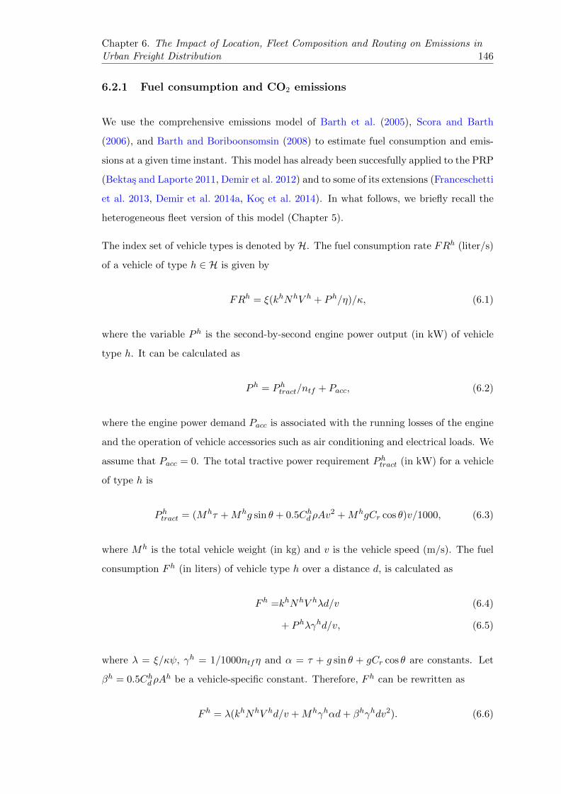
Chapter 6. The Impact of Location, Fleet Composition and Routing on Emissions inUrban Freight Distribution 146
6.2.1 Fuel consumption and CO2 emissions
We use the comprehensive emissions model of Barth et al. (2005), Scora and Barth
(2006), and Barth and Boriboonsomsin (2008) to estimate fuel consumption and emis-
sions at a given time instant. This model has already been succesfully applied to the PRP
(Bektas and Laporte 2011, Demir et al. 2012) and to some of its extensions (Franceschetti
et al. 2013, Demir et al. 2014a, Koc et al. 2014). In what follows, we briefly recall the
heterogeneous fleet version of this model (Chapter 5).
The index set of vehicle types is denoted by H. The fuel consumption rate FRh (liter/s)
of a vehicle of type h ∈ H is given by
FRh = ξ(khNhV h + P h/η)/κ, (6.1)
where the variable P h is the second-by-second engine power output (in kW) of vehicle
type h. It can be calculated as
P h = P htract/ntf + Pacc, (6.2)
where the engine power demand Pacc is associated with the running losses of the engine
and the operation of vehicle accessories such as air conditioning and electrical loads. We
assume that Pacc = 0. The total tractive power requirement P htract (in kW) for a vehicle
of type h is
P htract = (Mhτ +Mhg sin θ + 0.5Chd ρAv2 +MhgCr cos θ)v/1000, (6.3)
where Mh is the total vehicle weight (in kg) and v is the vehicle speed (m/s). The fuel
consumption F h (in liters) of vehicle type h over a distance d, is calculated as
F h =khNhV hλd/v (6.4)
+ P hλγhd/v, (6.5)
where λ = ξ/κψ, γh = 1/1000ntfη and α = τ + g sin θ + gCr cos θ are constants. Let
βh = 0.5Chd ρAh be a vehicle-specific constant. Therefore, F h can be rewritten as
F h = λ(khNhV hd/v +Mhγhαd+ βhγhdv2). (6.6)

Chapter 6. The Impact of Location, Fleet Composition and Routing on Emissions inUrban Freight Distribution 147
In this expression the first term khNhV hd/v is called the engine module, which is linear
in travel time. The second term Mhγhαijd is referred to as the weight module, and the
third term βhγhdv2 is the speed module, which is quadratic in speed. These functions
will be used in the objective function of the mathematical formulation in Section 6.3.
6.2.2 Vehicle types and characteristics
We consider three vehicle types of MAN (2015a), a major truck manufacturer whose
market share in Western Europe was around 16.3% in 2013 (Statista 2013). These
three vehicle types include two light duty (TGL) vehicles and one medium duty (TGM)
vehicle, classified as single-unit trucks by FHWA (2011). Table 6.1 lists the values of
the parameters (Demir et al. 2012, 2014a, Franceschetti et al. 2013, Koc et al. 2014)
common to all vehicle types, while Table 6.2 lists specific parameters (MAN 2015a,b,c)
for each vehicle type. We refer the reader to MAN (2015a,b,c) for further details on
TGL and TGM vehicles and their engines.
Table 6.1: Vehicle common parameters
Notation Description Typical values
ξ fuel-to-air mass ratio 1g gravitational constant (m/s2) 9.81ρ air density (kg/m3) 1.2041Cr coefficient of rolling resistance 0.01η efficiency parameter for diesel engines 0.45fc fuel and CO2 emissions cost (£/liter) 1.4κ heating value of a typical diesel fuel (kj/g) 44ψ conversion factor (g/s to L/s) 737ntf vehicle drive train efficiency 0.45θ road angle 0τ acceleration (m/s2) 0
The fuel consumption function (6.6) per unit distance travelled as a function of speed is
typically U-shaped (Figure 6.1) and results in an optimal speed that minimizes the fuel
consumption. This function, plotted in Figure 6.1 is the sum of two components, one
induced by (6.4) and the other by (6.5), for the three vehicle types considered in this
paper.

Chapter 6. The Impact of Location, Fleet Composition and Routing on Emissions inUrban Freight Distribution 148
Table6.2:
Veh
icle
spec
ific
para
met
ers
Not
ati
on
Des
crip
tion
Lig
ht
du
ty1
(L1)
Lig
ht
du
ty2
(L2)
Med
ium
du
ty(M
)
wh
curb
wei
ght
(kg)
3500
4500
5500
Qh
max
imu
mpay
load
(kg)
4000
7500
1250
0µh
veh
icle
fixed
cost
(£/d
ay)
4249
60kh
engin
efr
icti
onfa
ctor
(kj/
rev/l
iter
)0.
250.
230.
20Nh
engin
esp
eed
(rev
/s)
38.3
437
.45
36.6
7Vh
engin
ed
isp
lace
men
t(l
iter
)4.
54.
56.
9Ch d
coeffi
cien
tof
aero
dyn
amic
sd
rag
0.6
0.64
0.7
Ah
fron
tal
surf
ace
area
(m2)
7.0
7.4
8.0

Chapter 6. The Impact of Location, Fleet Composition and Routing on Emissions inUrban Freight Distribution 149
0.00
5.00
10.00
15.00
20.00
25.00
30.00
35.00
20 30 40 50 60 70 80 90 100 110Fu
el c
on
sum
pti
on (
L/
10
0 k
m)
Speed (km/h)
L1 L2 M
Figure 6.1: Fuel consumption as a function of speed
6.2.3 Speed zones
Road speed limits are commonly set by national or local governments (Wikipedia 2015).
They play a key role in ensuring the safety of road users and of the public at large (UK
Government 2014). In general, cities are divided into several speed zones which help
traffic flow more safely and efficiently. They also provide a reasonable balance between
the needs of drivers, pedestrians and cyclists who use public roads for travel, and the
concerns of residents who live along these roads (Oregon 2015b). Studies have been
performed in the United Kingdom by the Department for Transport (2013), in Canada
by the City of Ottawa Transportation Committee (2009) and in the United States by
the Oregon Department of Transportation (2015) on the best way to establish speed
zones. These studies indicate that setting reasonable vehicle speeds for a variety of
weather conditions results in fewer accidents. When reasonable speeds are imposed, less
overtaking occurs, and one also observes smaller delays and fewer rear-end collisions.
According to the above studies, speed zones in cities are generally classified under three
categories:
• 15 mph (25 km/h): alleys, narrow residential roadways,
• 20 mph (32 km/h): business districts, school zones,
• 25 mph (40 km/h): residential districts, public parks, ocean shores.

Chapter 6. The Impact of Location, Fleet Composition and Routing on Emissions inUrban Freight Distribution 150
Speed zones also yield environmental benefits. For example Kirkby (2002) states that
20 mph (32 km/h) speed zones, significantly improve the quality of life of the concerned
community, and encourage healthier and more sustainable transportation. This speed
limit favours slower driving, saves fuel and reduces pollution, unless an unnecessarily
low gear is used (DfT 2013).
6.2.4 Network structure
We consider cities in which distances are measured using the Taxicab geometry (see
Krause 2012). The Taxicab geometry is also known as the rectilinear distance, the L1
distance, the city block distance or the Manhattan distance. It implies that the shortest
path between two nodes is the sum of horizontal and vertical distances between them.
This metric is appropriate in several grid cities, such as Glasgow, Ottawa and Portland,
shown in Figure 6.2.
In the setting considered in this study, we assume that the city centre is divided into
several zones, each belonging to one of the three categories described in Section 6.2.3.
We also assume that speeds are deterministic and time-independent. Zone 1 corresponds
to the city centre, zone 2 is an outer urban area, and zone 3 corresponds to a suburb.
The index set of speed zones is denoted by Z. Let the zones be z1, z2, z3 ∈ Z and let
V1, V2, V3 be the fixed speeds in zones, where V1 < V2 < V3. Figure 6.3 illustrates a city
divided into three fixed speed zones. When a vehicle travels within the same zone z1, z2
or z3, its speed is equal to the speed of that zone. When it travels on the boundary of
two speed zones, it uses the faster speed of the two zones.
In a city, a shortest path between i and j is not necessarily a cheapest or a least polluting
path. In urban areas where a maximum speed limit of 40 km/h is imposed, a fastest
path is also a least-polluting path according to Figure 6.1. However, as in Ehmke et
al. (2014), this path is not always a shortest path. For example, consider the corners
(A,B,C,D) of zone 2 in Figure 6.3, and nodes i and j located in zone 3. When travelling
from i to j, a vehicle of type h may choose not to travel on a straight line from i to
j with speed V2 between points K and L, but may instead travel on the boundaries of
zone 2 with speed V3 ≤ 40 km/h to avoid driving at a slower speed through congested
traffic. A fastest path from customer i to j could well be (i,K,A,C, L, j) instead of
(i,K,L, j), particularly in urban settings.

Chapter 6. The Impact of Location, Fleet Composition and Routing on Emissions inUrban Freight Distribution 151
(a)
Gla
sgow
(b)
Ott
awa
(c)
Port
lan
d
Figure6.2:
Gri
dci
tyex
am
ple
s(G
oogle
Map
s2015)

Chapter 6. The Impact of Location, Fleet Composition and Routing on Emissions inUrban Freight Distribution 152
Zone 1
Zone 2
Zone 3
i j
A
B D
C
K L
Figure 6.3: Illustration of speed zones
Using equation (6.6), we now illustrate how the load on a vehicle can affect the calcu-
lation of the cheapest path between a node pair. In Figure 6.3, let us assume that the
total length of path (i,K,L, j) is 8 km, and for (i,K,A,C, L, j) is 9 km. When a vehicle
of type M going from i to j carries a load equal to 1000 kg, then the cost of (i,K,L, j) is
£1.85 and the cost of (i,K,A,C, L, j) is £1.95 with the former path being the cheaper
one. However, when the vehicle load is equal to 12500 kg, then the cost of (i,K,L, j)
is £2.20 and the cost of (i,K,A,C, L, j) is £2.05, where the cheapest path now is the
latter.
6.2.5 Depot costs
There are four main categories of depot or warehouse costs: handling, storage, operations
administration and general administrative expenses (see Ghiani et al. 2013). Storage
expenses are the cost of occupying a facility (Speh 2009). Depot location affects the
storage cost, e.g., locating a depot in the city centre (zone 1) is much more expensive
than locating it in an outer zone (zone 2 or 3).
6.3 Formal Problem Description and Mathematical For-
mulation
Our problem is defined on a complete directed graph G = (N ,A), where N = N0∪Nc is
a set of nodes in which N0 and Nc represent the potential depots and customer nodes,

Chapter 6. The Impact of Location, Fleet Composition and Routing on Emissions inUrban Freight Distribution 153
respectively. A storage capacity Dk and a fixed opening cost gk are associated with each
potential depot k ∈ N0. Each customer i ∈ Nc has a positive demand qi. The arc set
A is defined as A = (i, j) : i ∈ N , j ∈ N \ (i, j) : i ∈ N0, j ∈ N0, i 6= j. We assume
that an unlimited heterogeneous fleet of vehicles operates with various capacities and
vehicle-related costs. The index set of vehicle types is denoted by H. Let Qh and th
denote the capacity and fixed dispatch cost of a vehicle of type h ∈ H, respectively. Fuel
and CO2 emissions cost c(i, j, whi ) of traveling from node i to node j with a vehicle of
type h having a load equal to whi upon leaving i. This cost is calculated using equation
(6.6).
The problem consists of locating depots in a subset of N0, of assigning each customer
to a depot and of determining a set of vehicle routes such that all vehicles start and end
their routes at their depot, and the load of each vehicle does not exceed its capacity. The
objective is to minimize the total cost which is made up of three components: the depot
operating cost, the vehicle fixed cost, and the fuel and CO2 emissions cost. Furthermore,
the speed of a vehicle depends on the speeds of the zones it traverses while driving.
To formulate the problem, we define the following additional decision variables. Let xhij
be equal to 1 if a vehicle of type h ∈ H travels from node i to node j and to 0 otherwise.
Let uk be equal to 1 if depot k ∈ N0 is opened and to 0 otherwise. Let zik be equal
to 1 if customer i ∈ Nc is assigned to depot k ∈ N0 and to 0 otherwise. Let fhij be the
amount of commodity carried by a vehicle of type h from node i to node j.
The integer linear programming formulation of the problem is then:
Minimize∑k∈N0
gkuk +∑h∈H
∑k∈N0
∑j∈Nc
thxhkj +∑h∈H
∑(i,j)∈A
c(i, j, whi )xhij (6.7)
subject to
∑h∈H
∑j∈N
xhij = 1 i ∈ Nc (6.8)
∑h∈H
∑i∈N
xhij = 1 j ∈ Nc (6.9)∑h∈H
∑j∈N
fhji −∑h∈H
∑j∈N
fhij = qi i ∈ Nc (6.10)
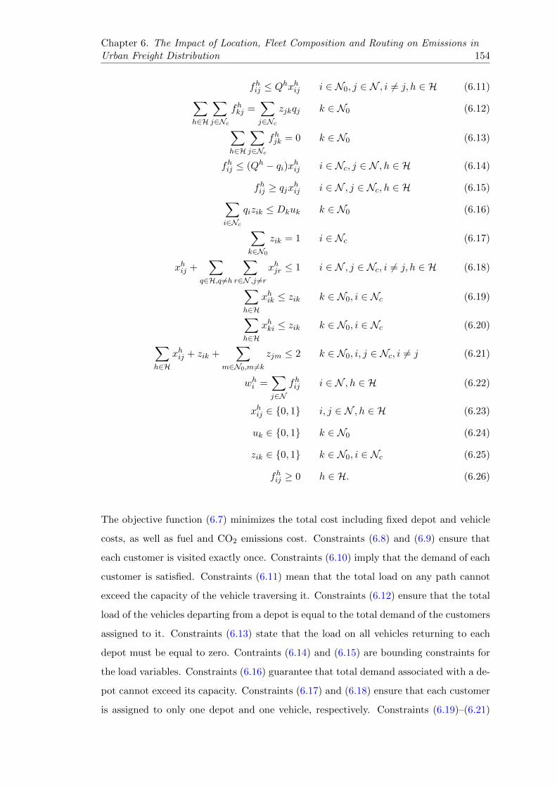
Chapter 6. The Impact of Location, Fleet Composition and Routing on Emissions inUrban Freight Distribution 154
fhij ≤ Qhxhij i ∈ N0, j ∈ N , i 6= j, h ∈ H (6.11)∑h∈H
∑j∈Nc
fhkj =∑j∈Nc
zjkqj k ∈ N0 (6.12)
∑h∈H
∑j∈Nc
fhjk = 0 k ∈ N0 (6.13)
fhij ≤ (Qh − qi)xhij i ∈ Nc, j ∈ N , h ∈ H (6.14)
fhij ≥ qjxhij i ∈ N , j ∈ Nc, h ∈ H (6.15)∑i∈Nc
qizik ≤ Dkuk k ∈ N0 (6.16)
∑k∈N0
zik = 1 i ∈ Nc (6.17)
xhij +∑
q∈H,q 6=h
∑r∈N ,j 6=r
xhjr ≤ 1 i ∈ N , j ∈ Nc, i 6= j, h ∈ H (6.18)
∑h∈H
xhik ≤ zik k ∈ N0, i ∈ Nc (6.19)∑h∈H
xhki ≤ zik k ∈ N0, i ∈ Nc (6.20)∑h∈H
xhij + zik +∑
m∈N0,m 6=kzjm ≤ 2 k ∈ N0, i, j ∈ Nc, i 6= j (6.21)
whi =∑j∈N
fhij i ∈ N , h ∈ H (6.22)
xhij ∈ 0, 1 i, j ∈ N , h ∈ H (6.23)
uk ∈ 0, 1 k ∈ N0 (6.24)
zik ∈ 0, 1 k ∈ N0, i ∈ Nc (6.25)
fhij ≥ 0 h ∈ H. (6.26)
The objective function (6.7) minimizes the total cost including fixed depot and vehicle
costs, as well as fuel and CO2 emissions cost. Constraints (6.8) and (6.9) ensure that
each customer is visited exactly once. Constraints (6.10) imply that the demand of each
customer is satisfied. Constraints (6.11) mean that the total load on any path cannot
exceed the capacity of the vehicle traversing it. Constraints (6.12) ensure that the total
load of the vehicles departing from a depot is equal to the total demand of the customers
assigned to it. Constraints (6.13) state that the load on all vehicles returning to each
depot must be equal to zero. Contraints (6.14) and (6.15) are bounding constraints for
the load variables. Constraints (6.16) guarantee that total demand associated with a de-
pot cannot exceed its capacity. Constraints (6.17) and (6.18) ensure that each customer
is assigned to only one depot and one vehicle, respectively. Constraints (6.19)–(6.21)

Chapter 6. The Impact of Location, Fleet Composition and Routing on Emissions inUrban Freight Distribution 155
forbid the creation of routes that do not start and end at the same depot. Constraints
(6.22) define the load of a vehicle of type h upon leaving node i as the total amount of
commodity on the arc (i, j) it uses to leave i. Finally, constraints (6.23)–(6.25) enforce
the integrality and non-negativity restrictions on the variables.
6.4 Description of the ALNS Metaheuristic
The mathematical formulation just presented is of large scale and cannot be solved
for practical instances. We have therefore devised a metaheuristic algorithm, called
pollution-and-location-heterogeneous adaptive large neighborhood search (P-L-HALNS),
to solve the problem. This algorithm is partly based on the ALNS framework of Demir
et al. (2012) which is initially put forward by Ropke and Pisinger (2006a,b) to solve
several variants of the VRP (see Laporte et al. 2014). This metaheuristic has since pro-
vided very good results on several complicated variants of the VRP (see Pisinger and
Ropke 2007, Koc et al. 2015), of the LRP (see Koc et al. 2016), and of the PRP (see
Demir et al. 2012, 2014a, Koc et al. 2014).
The P-L-HALNS consists of two basic procedures: removal or destroy, followed by in-
sertion or repair. In the removal procedure, n′ nodes are iteratively removed by destroy
operators and placed in the removal list, where n′ lies in the interval [bl, bu] for the de-
stroy operators. In the insertion procedure, the nodes of the removal list, are iteratively
inserted into a least-cost position of the incomplete solution by means of an insertion
operator. The removal and insertion operators are selected dynamically according to
their past performance. To this end, each operator is assigned a score which is increased
whenever it improves the current solution and is periodically reset to one. Simulated an-
nealing is used as an outer local search framework for the P-L-HALNS in order to define
the acceptance rules of candidate solutions. Simulated annealing acceptance criterion
has been recently shown to perform well for various routing problems (e.g., Pisinger and
Ropke 2007, Demir et al. 2012), which is the motivation to use the same approach in
our work.
In order to perform least-cost insertions, it is necessary to make use of cheapest path
values frequently during the course of the algorithm. We explain in Section 6.4.1 how

Chapter 6. The Impact of Location, Fleet Composition and Routing on Emissions inUrban Freight Distribution 156
these computations are handled in the ALNS metaheuristic. This is followed in Section
6.4.2 by an overview of the metaheuristic itself.
6.4.1 Cheapest path calculation
The number of undominated paths between any two nodes is finite, but the identification
of such paths is not trivial since the cost of a path depends (see equation (6.6)) on the
type of vehicle traveling a path from i to j, on its load upon leaving i, and on the speed
of each arc of the path. To overcome the complexity of this task, we introduce a heuristic
Cheapest Path Calculation procedure which computes only three paths between i
and j and selects the cheapest one. This procedure does not guarantee the calculation
of the minimum cost path over all possible paths, but is suitable for iterative use within
an algorithm like the P-L-HALNS described here.
Algorithm 1 presents this procedure for a node pair (i, j) which follows three steps.
In step 1 (lines 2–4), we find two shortest path between (i, j). According to Taxicab
geometry (see Section 6.2.4), if node i and j are not located at same horizontal or vertical
coordinate, there exist two shortest paths with the same length, but not necessarily with
the same cost for a vehicle with a fixed load, because of the possibility of cutting through
different zones. In this case, we identify the cheapest path p0 of the two paths and discard
the other one. In steps 2 and 3, we contort p0 to generate two alternative paths p1 and
p2. In step 2 (lines 5–7), path p1 follows the boundary of zone 1 on which it travels at
a speed V2 based on the assumption made in Section 6.2.3. Similarly, in step 3 (lines
8–10) path p2 follows the boundary of zone 2. We do not consider travel on or outside
the boundary of zone 3 as this is not defined. The algorithm then compares the costs
of p0, p1 and p2, and returns the cheapest path (line 11). In the P-L-HALNS, it should
be noted that we calculate the shortest paths (Step 1) between each pair of nodes as a
priori as in the VRP.
Figure 6.4 illustrates the Cheapest Path Calculation procedure for a given node
pair (i, j) and a vehicle with a fixed load traveling between these nodes. Figure 6.4.a
(Step 1) shows two paths, (i, A, j) and (i, B, j) that are the shortest with respect to
the Taxicab geometry and distance, but the cheapest path would always be (i, B, j)
since V2 < V3 ≤ 40 km/h. We then calculate the cost χ0 of p0 = (i, B, j). In Figure
6.4.b (Step 2), we first find the shortest path from node i to nearest point (A1) of zone

Chapter 6. The Impact of Location, Fleet Composition and Routing on Emissions inUrban Freight Distribution 157
Algorithm 1 Cheapest Path Calculation
1: Node i and node j(i, j ∈ N ). Let χ0, χ1, χ2 be the costs of paths p0, p1 and p22: Step 13: Find two shortest paths between (i, j) and choose the least cost path p0.4: Calculate the cost χ0 of path p0.5: Step 26: Find path p1 by contorting path p0 part of which lies on the border of zone 1 between
(i, j).7: Calculate the cost χ1 of path p1.8: Step 39: Find the path p2 by contorting path p0 part of which lies on the border of zone 2
between (i, j).10: Calculate the cost χ2 of path p2.11: Return Least cost path pk where k = arg min χ0, χ1, χ2.
1. We then find the shortest path, on the border of zone 1, from point A1 to nearest
point (B1) of zone 1 to node j. We finally find the shortest path from point B1 to node
j. As in Step 1, if there are two same length shortest paths between points, such as
(B1, B1a, j) and (B1, B1b, j), we select the cheapest one, in this case (B1, B1a, j). We
calculate the cost χ1 of p1 = (i, A1, B1, B1a, j). In Figure 6.4.c (Step 3), we first find
the shortest path from node i to nearest point (A2) of zone 2. We then find the shortest
path, on the border of zone 2, from point A2 to nearest point (B2) of zone 2 to node j.
We finally find the shortest path from point B2 to node j. We calculate the cost χ2 of
p2 = (i, A2, B2, j).
6.4.2 Overview of the metaheuristic
The general framework of the P-L-HALNS metaheuristic is sketched in Algorithm 2.
We now briefly explain its steps. Given the complexity of implementing the Cheapest
Path Calculation procedure at every step of the P-L-HALNS, we work with average
route demand lengths. At the beginning of the algorithm, we first define a set B of
average route demand levels. We know the total demand of customers as a priori. For
example, let |B| = 4 and total demand of customers is 2000 kg, which results in the
following intervals: level 1 ranges from zero to 500 kg, level 2 ranges from 501 to 1000
kg, level 3 ranges from 1001 to 1500 kg, and level 4 ranges from 1501 to 2000 kg. Let
υβhij be the fixed cost associated with the path for each average route demand level
β ∈ B and for each vehicle of type h ∈ H. The fixed costs υβhij are calculated at the
beginning of the algorithm (line 1). These fixed costs are used to compute the route

Chapter 6. The Impact of Location, Fleet Composition and Routing on Emissions inUrban Freight Distribution 158
Zon
e 1
Zon
e 2
Zon
e 3
i
jA
B
(a)
Sho
rtes
t p
ath
(b)
Sho
rtes
t p
ath
bas
ed o
n b
ord
er
of zon
e 1
(c)
Sho
rtes
t p
ath
bas
ed o
n b
ord
er
of zon
e 2
Ste
p 1
Ste
p 2
Ste
p 3
Zon
e 1
Zon
e 2
Zon
e 3
i
j
Zon
e 1
Zon
e 2
Zon
e 3
i
j
A1
B1a
A2
B2
B1b
B1
Figure6.4:
Illu
stra
tion
of
the
thre
esp
eed
zon
es

Chapter 6. The Impact of Location, Fleet Composition and Routing on Emissions inUrban Freight Distribution 159
costs quickly. During the algorithm, for each solution, average route demand calculated
as (total demand of customers)/(total number of vehicle routes). For example, let the
total demand of customers be 2000, |B| = 4 and the number of vehicle routes be three.
The average route demand is then 2000/3 and level β ∈ B is equal to 2.
An initial solution ω0 is generated by using a modified version of the classical Clarke
and Wright (1964) savings algorithm for the VRP (line 2). The selection probabilities
are initialized for each destroy and repair operator (line 3). In line 4, ωb is the best
solution found during the search, ωc is the current solution obtained at the beginning
of an iteration, and ωt is a temporary solution found at the end of the iteration which
can be discarded or become the current solution. The temperature is denoted by T , the
iteration counter is denoted by j, and the current and the best solutions are initially
set equal to the initial solution (line 4). The temperature T is initially set at c(ω0)P0,
where c(ω0) is the cost of initial solution and P0 is the initial temperature.
Every σ iterations, a diversification based removal operator is selected (lines 6–8) and
applied to ωc; otherwise an intensification based removal operator is selected (lines 9–
11). An insertion operator is then selected and applied to the destroyed solution, and a
feasible solution ωt is obtained (line 12).
The operators are applied using the average costs up until the counter p reaches ς,
following which the actual costs for ωc, ωt and ωb are calculated using the Cheapest
Path Calculation procedure (lines 13–15). Otherwise, the fixed costs are used to
compute c(ωt) (lines 16–18). If the cost of a repaired solution c(ωt) is less than that of the
current solution c(ωc), then ωc is replaced by ωt (lines 19–20). Otherwise, the probability
ϑ of accepting a non-improving solution is computed (line 21–22) as a function of the
current temperature. A random number ε is then generated in the interval [0, 1] (line 23).
If ε is less than ϑ, ωc is then replaced by ωt (lines 24–25). If the cost of ωc is less than that
of ωb, ωb is replaced by ωc (lines 26–27). The current temperature is gradually decreased
during the algorithm as δT (line 28), where 0 < δ < 1 is a fixed cooling parameter. The
probabilities are updated by means of an adaptive weight adjustment procedure (AWAP)
(line 29). When the maximal number $ iterations is reached, the algorithm terminates
(line 31) and returns the best found solution. For further information on the operators
and on other algorithmic details the reader is referred to Demir et al. (2012) and Koc
et al. (2015, 2016) and Chapters 3 and 4.
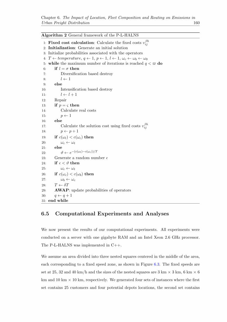
Chapter 6. The Impact of Location, Fleet Composition and Routing on Emissions inUrban Freight Distribution 160
Algorithm 2 General framework of the P-L-HALNS
1: Fixed cost calculation: Calculate the fixed costs υβhij2: Initialization: Generate an initial solution3: Initialize probabilities associated with the operators4: T ← temperature, q ← 1, p← 1, l← 1, ωc ← ωb ← ω0
5: while the maximum number of iterations is reached q < $ do6: if l = σ then7: Diversification based destroy8: l← 19: else
10: Intensification based destroy11: l← l + 1
12: Repair13: if p = ς then14: Calculate real costs15: p← 116: else17: Calculate the solution cost using fixed costs υβhij18: p← p+ 1
19: if c(ωt) < c(ωc) then20: ωc ← ωt21: else22: ϑ← e−(c(ωt)−c(ωc))/T
23: Generate a random number ε24: if ε < ϑ then25: ωc ← ωt26: if c(ωc) < c(ωb) then27: ωb ← ωc
28: T ← δT29: AWAP: update probabilities of operators30: q ← q + 131: end while
6.5 Computational Experiments and Analyses
We now present the results of our computational experiments. All experiments were
conducted on a server with one gigabyte RAM and an Intel Xeon 2.6 GHz processor.
The P-L-HALNS was implemented in C++.
We assume an area divided into three nested squares centered in the middle of the area,
each corresponding to a fixed speed zone, as shown in Figure 6.3. The fixed speeds are
set at 25, 32 and 40 km/h and the sizes of the nested squares are 3 km × 3 km, 6 km × 6
km and 10 km × 10 km, respectively. We generated four sets of instances where the first
set contains 25 customers and four potential depots locations, the second set contains
Chapter 6. The Impact of Location, Fleet Composition and Routing on Emissions inUrban Freight Distribution 161
50 customers and six potential depots locations, the third set contains 75 customers
and eight potential depots locations, and the fourth set contains 100 customers and 10
potential depots depots. Each set includes three subsets: 1) customers concentrated in
the city centre, denoted by CC, 2) customers concentrated in the outer city area and in
the suburb, denoted by SU, and 3) customers located randomly, denoted by R. These
three subsets of benchmark instances are illustrated in Figure 6.5. These configurations
cover a wide variety of realistic urban settings.
Each subset includes five instances, resulting in a total of 60 instances. To generate the
depot characteristics, we used a procedure similar to that used for the standard LRP
benchmark instances (see Barreto 2004, Albareda-Sambola et al. 2005, Prodhon 2006).
We also further explore the effect of variations in depot costs in Section 6.5.4. The
customer demands and the depot capacities (in kg) were randomly generated using a
uniform distribution in the range [100, 1100] and [10000, 15000], respectively. The fixed
depot costs are dependent on their location, i.e., zone 1 has the highest fixed cost (per
depot £5000/day), followed by zone 2 (per depot £3500/day) and finally zone 3 (per
depot £2000/day). All costs relate to the same planning horizon.
The parameters used in the P-L-HALNS are provided in Table 6.3. All algorithmic
parametric values, except ς and σ, are as described in Demir et al. (2012), who applied
an extensive meta-calibration procedure to generate effective parameter values for their
ALNS heuristic for the PRP. During the experiments, ten runs were performed for each
instance and the result of the best one was retained.
The aim of the computational experiments is fivefold: 1) to solve the problem described
in Section 6.3, 2) to empirically calculate the savings that could be achieved by using a
comprehensive objective function instead of using individual functions for each perfor-
mance indicator, 3) to analyze the effect of variations in potential depot locations and
customer distribution, 4) to investigate the effect of variations in depot costs, and 5) to
quantify the benefits of using a heterogeneous fleet over a homogeneous one.
6.5.1 Results obtained on the test instances
This section presents the results obtained by P-L-HALNS on the 25-, 50-, 75- and 100-
customer instances. Table 6.4 presents the average results for each instance set where the

Chapter 6. The Impact of Location, Fleet Composition and Routing on Emissions inUrban Freight Distribution 162
(a)
CC
(b)
SU
(c)
R
Depot
Depot
Depot
Depot
Depot
Depot
Depot
Depot
Depot
Figure6.5:
Geo
grap
hic
al
cust
om
erd
istr
ibu
tion
inth
eb
ench
mark
inst
an
ces

Chapter 6. The Impact of Location, Fleet Composition and Routing on Emissions inUrban Freight Distribution 163
Table 6.3: Parameters used in the P-L-HALNS
Description Typical values
Total number of iterations ($) 25000Number of iterations for roulette wheel 450Roulette wheel parameter 0.1New global solution 1Better solution 0Worse solution 5Startup temperature parameter (P0) 100Cooling parameter (δ) 0.999Lower limit of removable nodes 5-20% of |Nc|Upper limit of removable nodes 12-30% of |Nc|First shaw parameter 0.5Second shaw parameter 0.15Third shaw parameter 0.25Noise parameter 0.1Route cost calculation parameter (ς) 100Diversification parameter (σ) 50
columns display the average distance (km), CO2 emissions (kg), fuel and CO2 emissions
cost (£), depot cost (£), vehicle cost (£), total cost (£) and time (s). We also report the
average number of opened depots for each subset. In this column, the first, second and
third elements within the parentheses represent the number of opened depots in zone
1, 2 and 3, respectively. To evaluate the environmental impact of the solutions, we also
report the average amount of CO2 emissions (in kg) based on the assumption that one
liter of gasoline contains 2.32 kg of CO2 (Coe 2005). For detailed results, the reader is
referred to Tables A.1–A.4 in the Appendix.
From Table 6.4, it is clear that the total cost is dominated by the large depot costs
which force the P-L-HALNS to first minimize the number of depots, then minimize the
vehicle fixed costs, and lastly fuel and CO2 emission costs.
6.5.2 The effect of the various cost components of the objective func-
tion
In this section, we analyze the implications of using different objectives on a number of
performance measures. To this end, we have conducted experiments using four special
cases of the objective function, which are presented in the first column of Table 6.5. The
experiments were conducted on all 100-customer R, SU and CC instances. In the first
version, we only consider minimizing the fuel and CO2 emissions costs (F). This setting

Chapter 6. The Impact of Location, Fleet Composition and Routing on Emissions inUrban Freight Distribution 164
Table6.4:
Ave
rage
resu
lts
on
the
inst
an
ces
Inst
ance|N
c||N
0|
Op
ened
Tot
ald
ista
nce
CO
2em
issi
ons
Fu
elan
dC
O2
Dep
otco
stV
ehic
leco
stT
otal
cost
Tim
ed
epots
(km
)(k
g)em
issi
ons
cost
s(£
)(£
)(£
)(£
)(s
)
CC
25
25
4(1
.2,
0.2,
0.5)
37.4
021
.56
13.0
179
00.0
010
6.20
8019
.21
5.46
SU
25
25
4(0
.4,0
.8,0
.6)
56.0
120
.63
12.4
554
00.0
010
2.60
5515
.05
5.44
R25
254
(0.4
,0.8
,0.4
)64
.78
19.4
811
.76
5600
.00
104.
0057
15.7
65.
41C
C50
50
6(1
.6,0
.6,0
.8)
80.6
623
.68
14.2
911
700.
0017
5.60
1188
9.88
32.1
1S
U50
50
6(0
.4,0
.6,2
.0)
125.
1521
.44
12.9
481
00.0
017
5.60
8288
.53
31.0
0R
5050
6(0
.2,1
.0,1
.8)
128.
6023
.40
14.1
281
00.0
016
9.00
8283
.12
31.5
3C
C75
75
8(2
.2,1
.0,0
.8)
106.
1428
.43
17.1
616
100.
0025
6.80
1637
3.96
68.2
1S
U75
75
8(0
.0,2
.0,2
.0)
200.
3932
.73
19.7
511
300.
0028
8.80
1160
8.54
64.2
9R
7575
8(0
.0,2
.2,1
.8)
197.
8938
.22
23.0
611
000.
0030
0.00
1132
3.04
64.0
2C
C100
100
10(2
.6,1
.4,1
.4)
140
.24
43.6
126
.31
2070
0.00
358.
2021
084.
5216
9.51
SU
100
100
10(0
.0,2
.2,3
.0)
244
.44
42.0
225
.35
1490
0.00
397.
4015
322.
7615
1.15
R10
010
010
(0.0
,3.0
,2.2
)259
.42
54.6
632
.98
1360
0.00
395.
8014
028.
7815
8.13

Chapter 6. The Impact of Location, Fleet Composition and Routing on Emissions inUrban Freight Distribution 165
also implies minimizing CO2 since emissions are proportional to fuel consumption. We
then consider the objective of minimizing only the depot cost (D) and the vehicle fixed
cost (V) in the second and third versions, respectively. The next objective corresponds
to that of the HVRP which jointly minimizes distance and vehicle fixed costs (DV).
Finally, we present the comprehensive objective of minimizing the total cost function
(T) as defined by (6.7).
Table 6.6 presents the average deviations of each component from the smallest value of
each column. For example, in the case of the R100 instances, the minimum average value
for objective D is £13,600 across the five objective functions, but objective V yields a
solution in which the average depot cost is £18,289.66, corresponding to an increase of
34.48% over the former. For the R100, SU100 and CC100 instances, it is clear that
objective F results in a poor total cost performance, yielding a 20.39%, 33.66% and
6.69% average increases over the value found through objective T, respectively. In the
case of the R100 instances, this increase is more substantial for objective V, which is
on average 33.06% higher. For the R100, SU100 and CC100 instances, as for emissions,
objective F yields an increase of 20.91%, 18.18% and 6.67% in depot cost over the
value provided by objective D, respectively. For the R100, SU100 and CC100 instances,
objective DV performs very poorly on all cost components, yielding average increases of
151.36%, 151.67% and 64.00%, respectively. These results indicate that traveling on a
shortest path does not always result in a cheapest solution. In urban settings, due to the
effect of speed zones on the objective function, longer paths outside the city centre have
the potential to decrease the solution cost, a situation that was explained in Section 6.2.
Maden et al. (2010) reached a similar conclusion relative to long-haul transportation.
6.5.3 The effect of variations in depot and customer locations
In this section, we investigate the effect of the variations in potential depot locations
and customer distribution. To this end, we have selected five R type instances with 100
customers and 10 potential depots. We consider three variations, namely all depots are
potentially located in zone 1, in zone 2, and in zone 3, respectively. Customer locations
are kept the same across all variations. In the tables, the columns DevCO2 and DevT
show the deviations in CO2 emissions (in kg) and in total cost (£) between the various
depot or customer location cases and the base case.

Chapter 6. The Impact of Location, Fleet Composition and Routing on Emissions inUrban Freight Distribution 166
Table6.5:
Th
eeff
ect
of
cost
com
pon
ents
:ob
ject
ive
fun
ctio
nva
lues
.
Ob
ject
ive
Op
ened
Tota
ldis
tan
ceC
O2
emis
sion
sF
uel
and
CO
2D
epot
cost
Veh
icle
cost
Tota
lco
stdep
ots
(km
)(k
g)
emis
sion
sco
sts
(£)
(£)
(£)
(£)
R10
0in
stan
ces
Fuel
and
CO
2em
issi
ons
cost
(F)
(1.0
,3.1
,1.0
)257
.66
30.
5018
.40
16443
.79
363
.51
168
89.1
0D
epot
cost
(D)
(0.0
,3.1
,2.2
)238
.34
52.
4131
.63
13600
.00
399
.97
140
30.0
0V
ehic
lefixed
cost
(V)
(1.1
,3.2
,2.1
)248
.40
36.
3421
.93
18289
.66
356
.22
186
66.4
6D
ista
nce
and
vehic
lefixed
cost
(DV
)(4
.0,3
.1,3
.2)
333
.19
119
.59
72.1
734
234
.48
962
.42
352
63.3
1T
otal
cost
(T)
(0.0
,3.0
,2.2
)259
.42
54.
6632
.98
13600
.00
395
.80
140
28.7
8
SU
100
inst
ance
sF
uel
and
CO
2em
issi
ons
cost
(F)
(1.1
,3.0
,2.0
)244
.44
42.
0225
.35
20037
.93
416
.03
204
80.9
5D
epot
cost
(D)
(0.0
,3.2
,3.0
)304
.11
43.
6226
.32
16955
.17
498
.82
174
80.0
1V
ehic
lefixed
cost
(V)
(1.0
,3.1
,2.0
)250
.09
62.
9137
.96
20037
.93
361
.18
204
38.2
9D
ista
nce
and
vehic
lefixed
cost
(DV
)(4
.0,3
.2,3
.1)
340
.56
92.
4855
.81
37506
.90
999
.71
385
62.3
0T
otal
cost
(T)
(0.0
,2.2
,3.0
)248
.49
43.
5226
.26
14900
.00
397
.40
153
22.7
6
CC
100
inst
ance
sF
uel
and
CO
2em
issi
ons
cost
(F)
(3.0
,2.0
,1.1
)117
.68
36.
1521
.82
22080
.00
369
.49
224
94.3
5D
epot
cost
(D)
(3.1
,1.2
,2.1
)161
.18
69.
3641
.85
20700
.00
408
.49
211
40.9
4V
ehic
lefixed
cost
(V)
(3.0
,2.2
,1.1
)124
.22
43.
9726
.53
22080
.00
358
.20
224
67.6
2D
ista
nce
and
vehic
lefixed
cost
(DV
)(4
.3,3
.1,3
.0)
256
.51
86.
3052
.08
33580
.00
991
.46
345
79.2
2T
otal
cost
(T)
(2.6
,1.4
,1.4
)140
.24
43.
6126
.31
20700
.00
358
.20
210
84.5
2

Chapter 6. The Impact of Location, Fleet Composition and Routing on Emissions inUrban Freight Distribution 167
Table6.6:
Th
eeff
ect
of
cost
com
pon
ents
:p
erce
nt
dev
iati
on
from
the
min
imu
mva
lue.
Ob
ject
ive
Tot
ald
ista
nce
CO
2em
issi
ons
Fu
elan
dC
O2
Dep
otco
stV
ehic
leco
stT
otal
cost
(km
)(k
g)em
issi
ons
cost
s(£
)(£
)(£
)(£
)
R100
inst
an
ces
Fu
elan
dC
O2
emis
sion
sco
st(F
)8.
110.
000.
0020
.91
2.05
20.3
9D
epot
cost
(D)
0.00
71.8
671
.86
0.00
12.2
80.
01V
ehic
lefi
xed
cost
(V)
4.22
19.1
519
.15
34.4
80.
0033
.06
Dis
tan
cean
dve
hic
lefi
xed
cost
(DV
)39
.79
292.
1329
2.13
151.
7217
0.18
151.
36T
otal
cost
(T)
8.84
79.2
279
.21
0.00
11.1
10.
00
SU
100
inst
ance
sF
uel
an
dC
O2
emis
sion
sco
st(F
)0.
000.
000.
0018
.18
15.1
933
.66
Dep
ot
cost
(D)
24.4
13.
823.
820.
0038
.11
14.0
8V
ehic
lefi
xed
cost
(V)
2.31
49.7
349
.73
18.1
80.
0033
.39
Dis
tan
cean
dve
hic
lefi
xed
cost
(DV
)39
.32
120.
1212
0.12
121.
2117
6.79
151.
67T
otal
cost
(T)
1.66
3.57
3.57
0.00
10.0
30.
00
CC
100
inst
ance
sF
uel
an
dC
O2
emis
sion
sco
st(F
)0.
000.
000.
006.
673.
156.
69D
epot
cost
(D)
36.9
791
.85
91.8
50.
0014
.04
0.27
Veh
icle
fixed
cost
(V)
5.56
21.6
321
.63
6.67
0.00
6.56
Dis
tan
cean
dve
hic
lefi
xed
cost
(DV
)11
7.97
138.
7313
8.73
62.2
217
6.79
64.0
0T
otal
cost
(T)
19.1
820
.62
20.6
20.
000.
000.
00

Chapter 6. The Impact of Location, Fleet Composition and Routing on Emissions inUrban Freight Distribution 168
Table6.7:
Th
eeff
ect
of
vari
ati
on
sin
dep
ot
loca
tion
.
Inst
ance
All
dep
ots
inzo
ne
1A
lldep
ots
inzo
ne
2A
lldep
ots
inzo
ne
3M
ixC
O2
(kg)
Tot
alco
st(£
)D
evCO
2D
evT
CO
2(k
g)T
otal
cost
(£)
DevCO
2D
evT
CO
2(k
g)T
otal
cost
(£)
DevCO
2D
evT
CO
2(k
g)
Tota
lco
st(£
)
R10
01
110.
6825
390.
303.
4541
.14
90.1
017
866.
20−
18.6
016
.35
77.3
610
367.
00−
38.1
2−
44.1
510
6.86
14944.5
0R
100
252
.29
2546
4.60
16.5
047
.34
43.2
617
917.
10−
0.93
25.1
540
.40
1046
1.00
−8.
06−
28.1
943
.66
13410.3
0R
100
350
.77
2542
1.60
14.2
347
.19
38.6
217
907.
30−
12.7
525
.03
40.7
710
422.
60−
6.82
−28
.80
43.5
513
424.3
0R
100
454
.14
2546
5.70
21.4
447
.34
40.9
217
946.
70−
3.94
25.2
838
.28
1048
8.10
−11
.12−
27.8
642
.53
13409.7
0R
100
577
.70
2538
8.90
52.8
041
.10
35.6
617
866.
50−
2.86
16.3
035
.20
1036
6.30
−4.
20−
44.2
736
.68
14955.1
0
Avg
(%)
21.6
844
.82
−7.
8221
.62
−13
.66−
34.6
5

Chapter 6. The Impact of Location, Fleet Composition and Routing on Emissions inUrban Freight Distribution 169
We first report in Table 6.7 the effect of varying the depot locations. Table 6.7 shows that
when all depots are located in zone 1, CO2 emissions increase by 21.68%. When they
are located in zones 2 and 3, CO2 emissions decrease by 7.82% and 13.66%, respectively.
Table 6.7 suggests that the average increase in the total cost is 44.82% and 21.62% on
average when all depots are located in zone 1 and 2, respectively over the base case.
When all the depots are located in zone 3, the total cost decreases by about 34.65%
on average. This analysis indicates that in terms of cost, it is preferable to locate the
depots in suburban areas rather than in the city centre when the customers are uniformly
distributed, i.e., for R instances. This also helps reduce congestion in city centres. A
similar observation was made by Dablanc (2014) who conducted an empirical study
on depot location in the Los Angeles area and concluded that warehouses moved out
an average of six miles from the area barycentre between 1998 and 2009. Dablanc’s
findings are mainly a consequence of the fact that land is cheaper in the suburbs than in
inner-cities, which translates into lower depot costs. Our study goes one step further in
that it shows that locating depots in peripheral zones also helps reduce pollution since
more travel can be made at an optimal speed. Locating depots outside the city centre
translates into larger driving distances to the inner city customers but yields overall
economic and environmental benefits.
We now analyze the effect of variations in customer locations. Table 6.8 provides a
comparison of three variations, namely all customers located in zone 1, all customers
located in zone 2, and all customers located in zone 3. The depot locations are kept the
same across all variations. Table 6.8 shows that when all customers are located in zone
3, CO2 emissions increase by 11.42%. On the other hand, when all customers are located
in zone 1 and 2, CO2 emissions decrease by 38.97% and 50.14%, respectively. Table 6.8
suggests that the average total cost increase over the base case is 38.16%, 6.04% and
8.12% on average when all customers are located in zone 1, 2 and 3, respectively. For
the case where all customers are located in zone 1, 2 and 3, the increase in the total cost
ranges from 33.25% to 41.50%, from −0.33% to 10.36%, and from −0.29% to 20.57%,
respectively. Our results suggest that when all customers are located only in the city
centre this is always more expensive than for the other settings.

Chapter 6. The Impact of Location, Fleet Composition and Routing on Emissions inUrban Freight Distribution 170
Table6.8:
Th
eeff
ect
of
vari
ati
on
sin
cust
om
erlo
cati
on
.
Inst
ance
All
cust
omer
sin
zone
1A
llcu
stom
ers
inzo
ne
2A
llcu
stom
ers
inzo
ne
3M
ixC
O2
(kg)
Tot
alco
st(£
)D
evCO
2D
evT
CO
2(k
g)T
otal
cost
(£)
DevCO
2D
evT
CO
2(k
g)T
otal
cost
(£)
DevCO
2D
evT
CO
2(k
g)T
otal
cost
(£)
R10
01
63.6
614
2241
1.30
−67
.86
33.3
265
.15
1490
6.20
−64
.02−
0.26
107.
5514
912.
700.
64−
0.21
106
.86
14944.5
0R
100
229
.630
822
877.
90−
47.3
541
.38
27.1
814
938.
40−
60.6
110
.23
46.5
514
950.
106.
2210
.30
43.
6613
410.3
0R
100
330
.663
2287
8.50
−42
.02
41.3
225
.80
1494
8.60
−68
.83
10.2
047
.04
1495
4.40
7.42
10.2
343.
5513
424.3
0R
100
433
.763
122
922.
40−
25.9
841
.50
40.1
614
959.
30−
5.92
10.3
654
.87
1688
2.10
22.4
820
.57
42.
5313
409.7
0R
100
532
.847
722
406.
20−
11.6
633
.25
24.2
414
905.
60−
51.3
4−
0.33
46.0
514
911.
8020
.35
−0.
2936.
6814
955.1
0
Avg
(%)
−38
.97
38.1
6−
50.1
46.
0411
.42
8.12

Chapter 6. The Impact of Location, Fleet Composition and Routing on Emissions inUrban Freight Distribution 171
6.5.4 The effect of variations in depot costs
In practice, it is very difficult to estimate depot costs because these depend on factors
such as land and building cost, staffing and technology. In general, these factors are
highly variable and hard to quantify. In our benchmark instances, the depot costs are
high with respect to other costs and dependent on their location, i.e., every zone has its
own fixed depot cost. We now investigate the effect of variations in depot costs.
Our first experiments analyze the effect of same depot costs on opened depots. To this
end, we have selected five R type instances with 100 customers and 10 depots. We
consider five versions in which all depot costs are fixed at £5000, £3500, £2000, £1000
and £500 per day in all zones. Table 6.9 shows that when the variable depot cost (Mix)
is used for each zone, 5.5 depots are opened in zones 2 and 3 on average. For the £5000,
£3500, £2000, £1000 and £500 fixed costs, 3.4, 3.8, 3.8, 4.0 and 4.0 depots are opened
in zones 2 and 3 on average. On the other hand, for these three fixed costs variants,
1.6, 1.2, 1.4, 1.2 and 0.0 depots are opened in zone 1 on average. The average number
of opened depots in the city centre is always lower than the total of number of opened
depots in the outer urban area and in the suburb. Our results clearly show that even if
depot costs are the same in everywhere, it is still preferable to locate depots outside the
city centre because of the pollution aspect (see Section 6.5.3).
Our next experiments investigate the effect of decreasing the variable depot costs. To
this end, we have conducted four series of tests on all 100-customer CC, SU and R
instances using our original variable depot costs structure. In these tests, we decrease
the depot costs by 90%, 70%, 50% and 30%, respectively. For example, decreasing the
depot cost by 90% means that the depot costs in zone 1, 2 and 3 are £500, £350 and
£200, respectively. Looking at the results presented in Table 6.10, we observe no change
in the locations of opened depots for all instances and for all variations. For example,
for the CC100 instances, when we decrease depot costs by 90%, 70%, 50% and 30%, it
is still preferable to open three depots in zone 1, one depot in zone 2 and two depots in
zone 3. Even though customers are concentrated in the city centre, half of the depots are
still located in the suburb. When we look at the SU100 instances, no depot is located
in city centre, but six depots are located in outer city area and in the suburb. The
R100 instances follows the same pattern with no depot located in the city centre, but
five depots located in the outer city area and in the suburb. Again, these results clearly
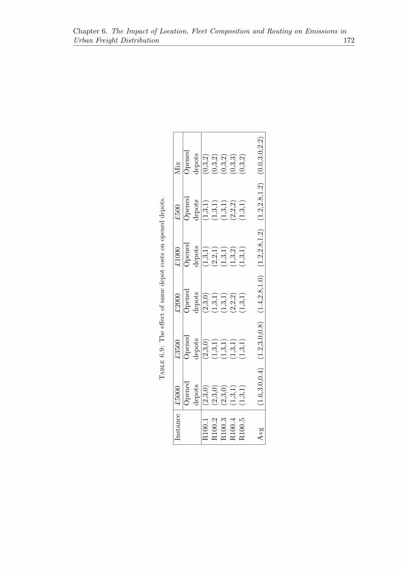
Chapter 6. The Impact of Location, Fleet Composition and Routing on Emissions inUrban Freight Distribution 172
Table6.9:
Th
eeff
ect
of
sam
ed
epot
cost
son
op
ened
dep
ots
.
Inst
ance
£5000
£35
00£
2000
£10
00£
500
Mix
Op
ened
Op
ened
Op
ened
Op
ened
Op
ened
Op
ened
dep
ots
dep
ots
dep
ots
dep
ots
dep
ots
dep
ots
R100
1(2
,3,0
)(2
,3,0
)(2
,3,0
)(1
,3,1
)(1
,3,1
)(0
,3,2
)R
100
2(2
,3,0
)(1
,3,1
)(1
,3,1
)(2
,2,1
)(1
,3,1
)(0
,3,2
)R
100
3(2
,3,0
)(1
,3,1
)(1
,3,1
)(1
,3,1
)(1
,3,1
)(0
,3,2
)R
100
4(1
,3,1
)(1
,3,1
)(2
,2,2
)(1
,3,2
)(2
,2,2
)(0
,3,3
)R
100
5(1
,3,1
)(1
,3,1
)(1
,3,1
)(1
,3,1
)(1
,3,1
)(0
,3,2
)
Avg
(1.6
,3.0
,0.4
)(1
.2,3
.0,0
.8)
(1.4
,2.8
,1.0
)(1
.2,2
.8,1
.2)
(1.2
,2.8
,1.2
)(0
.0,3
.0,2
.2)
Chapter 6. The Impact of Location, Fleet Composition and Routing on Emissions inUrban Freight Distribution 173
show that no matter what the depot cost is, it is still preferable to locate the depots
outside the city centre due to the impact of their location on CO2 emissions.
6.5.5 The effect of fleet composition
This section analyzes the benefit of using a heterogeneous fleet of vehicles over a ho-
mogenous one. To this end, we have conducted three sets of experiments on three
100-customer instances, each using a unique vehicle type, i.e., only light duty 1 (L1),
only light duty 2 (L2) and only medium duty (M). This results in three instances of
the homogeneous version of the problem which are solved with the P-L-HALNS. Table
6.11 provides the results of this comparison. The columns DevCO2 and DevT show the
deviations in CO2 emissions (in kg) and in total cost between the various homogeneous
cases and the heterogeneous case.
Table 6.11 shows that for the CC instances, CO2 emissions increase by 29.16% when
L1 vehicles are used, and decrease by 10.54% and 12.45% when L2 and M vehicles are
used, respectively. The results of the SU and R instances yield similar values for CO2
emissions, which decrease by L1 and L2 vehicles and increase by M type vehicles. Table
6.11 indicates that the average increase in total cost for the CC instances is 17.00%,
7.06% and 1.87%, for the SU instances 5.53%, 4.45% and 4.67%, for the R instances
12.09%, 10.21% and 10.44% when using L1, L2 and M homogeneous fleet over the
heterogeneous case, respectively. These results imply that if one is to use a homogeneous
fleet, it is preferable to use vehicles of type M in city centres (CC). For the suburban
(SU) and randomly distributed customer (R) location scenarios, homogeneous vehicles
of types L2 and M yield almost the same average total cost increase. This result shows
that both the L2 and M vehicles are suitable for the SU and R instances. Our results
also show that using a heterogeneous vehicle fleet is preferable to using a homogeneous
one since the total cost decreases by about 17% at most. For urban settings or short-
haul transportation, using a heterogeneous fleet does not seem to have same impact on
the total cost as in long-haul transportation. Chapter 5 have indeed shown that using
a heterogeneous fleet can decrease the total cost by up to 25% in inter-city travel.
Our final experiments aim at providing some insight into the capacity utilization of the
vehicle fleet, both for the homogenous and the heterogeneous cases, and also into the
capacity utilization of the depots. In Table 6.12, we present the capacity utilizations for

Chapter 6. The Impact of Location, Fleet Composition and Routing on Emissions inUrban Freight Distribution 174
Table6.10:
Th
eeff
ect
of
dec
reasi
ng
the
dep
ot
cost
s.
Inst
ance
Ch
an
gein
Op
ened
Tot
ald
ista
nce
CO
2em
issi
ons
Fu
elan
dC
O2
Dep
otco
stV
ehic
leco
stT
otal
cost
dep
ot
cost
(%)
dep
ots
(km
)(k
g)em
issi
ons
cost
s(£
)(£
)(£
)(£
)
CC
100
−90%
(3,1
,2)
106.
7463
.93
38.5
820
70.0
035
8.20
2424
.02
SU
100
−90%
(0,3
,3)
255.
7124
.29
14.6
616
95.5
237
2.56
2080
.63
R100
−90%
(0,3
,2)
250.
7034
.63
20.9
013
60.0
039
5.80
1756
.22
CC
100
−70%
(3,1
,2)
155.
1171
.33
43.0
562
10.0
035
8.20
6576
.01
SU
100
−70%
(0,3
,3)
268.
6745
.66
27.5
650
86.5
537
2.56
5485
.30
R100
−70%
(0,3
,2)
279.
4825
.98
15.6
840
80.0
040
7.26
4479
.27
CC
100
−50%
(3,1
,2)
129.
8266
.44
40.0
910
350.
0035
8.20
1072
2.59
SU
100
−50%
(0,3
,3)
239.
5944
.95
27.1
284
77.5
937
2.56
8876
.44
R100
−50%
(0,3
,2)
258.
5554
.19
32.7
068
00.0
039
5.80
7222
.50
CC
100
−30%
(3,1
,2)
115.
7960
.75
36.6
614
490.
0035
8.20
1486
8.95
SU
100
−30%
(0,3
,3)
247.
6213
.93
8.41
1186
8.62
372.
5612
249.
06R
100
−30%
(0,3
,2)
253.
9952
.10
31.4
495
20.0
039
9.97
9946
.26
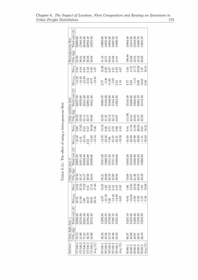
Chapter 6. The Impact of Location, Fleet Composition and Routing on Emissions inUrban Freight Distribution 175
Table6.11:
Th
eeff
ect
of
usi
ng
ah
eter
ogen
eou
sfl
eet
Inst
ance
Only
ligh
tduty
1O
nly
ligh
tduty
2O
nly
med
ium
duty
Het
erog
eneo
us
flee
tC
O2
(kg)
Tot
alco
st(£
)D
evCO
2D
evT
CO
2(k
g)T
otal
cost
(£)
DevCO
2D
evT
CO
2(k
g)T
otal
cost
(£)
DevCO
2D
evT
CO
2(k
g)
Tota
lco
st(£
)
CC
100
150
.12
2628
6.20
46.5
514
.94
28.5
623
007.
20−
16.4
80.
6029
.33
2287
7.70
−14
.22
0.04
34.
20228
69.6
0C
C10
02
51.8
022
745.
3041
.40
27.3
235
.47
2101
1.40
−3.
1917
.62
32.8
219
379.
80−
10.4
38.
4836.
64178
64.1
0C
C10
03
71.2
426
251.
501.
6917
.02
55.1
722
508.
80−
21.2
50.
3455
.14
2244
1.20
−21
.29
0.04
70.
06224
33.3
0C
C10
04
46.7
824
784.
2022
.27
8.31
39.5
023
013.
803.
240.
5735
.77
2298
1.60
−6.
520.
4338.
26228
83.1
0C
C10
05
52.0
622
745.
4033
.91
17.4
133
.04
2250
9.90
−15
.02
16.2
035
.08
1944
1.20
−9.
770.
3538.
88193
72.5
0A
vg
(%)
29.1
617
.00
−10
.54
7.06
−12
.45
1.87
SU
100
140
.33
1728
0.30
−2.
6715
.91
35.3
117
011.
30−
14.7
814
.10
42.5
916
885.
702.
7713
.26
41.
44149
09.0
0SU
100
234
.32
1523
4.70
−21
.48
1.89
32.6
614
960.
70−
25.2
80.
0641
.37
1544
5.00
−5.
363.
2943.
71149
52.4
0SU
100
341
.72
1573
9.20
7.96
5.23
35.5
915
511.
50−
7.90
3.71
43.1
215
446.
0011
.60
3.27
38.
64149
56.3
0SU
100
438
.36
1729
5.10
−14
.16
2.42
35.0
017
511.
10−
21.6
73.
7042
.15
1744
5.40
−5.
673.
3144.
68168
87.0
0SU
100
535
.40
1523
5.40
−14
.92
2.19
29.8
315
008.
00−
28.3
10.
6642
.67
1494
3.30
2.55
0.23
41.
61149
09.1
0A
vg
(%)
−9.
055.
53−
19.5
94.
451.
184.
67
R10
01
98.2
715
237.
10−
8.04
1.96
73.6
815
010.
30−
31.0
50.
4411
1.96
1514
5.30
4.77
1.34
106
.86
149
44.5
0R
100
238
.89
1527
9.50
−10
.92
13.9
434
.67
1501
0.90
−20
.59
11.9
444
.55
1500
6.90
2.03
11.9
143.
66134
10.3
0R
100
340
.07
1528
0.20
−8.
0013
.82
31.3
615
008.
90−
27.9
911
.80
43.0
515
004.
20−
1.15
11.7
743.
55134
24.3
0R
100
438
.81
1727
9.40
−8.
7628
.86
33.7
417
010.
40−
20.6
826
.85
42.5
716
885.
700.
0925
.92
42.
53134
09.7
0R
100
536
.10
1523
5.80
−1.
571.
8832
.49
1496
0.60
−11
.41
0.04
40.5
915
144.
5010
.65
1.27
36.
68149
55.1
0A
vg
(%)
−7.
4612
.09
−22
.34
10.2
13.
2810
.44

Chapter 6. The Impact of Location, Fleet Composition and Routing on Emissions inUrban Freight Distribution 176
the three homogeneous settings of Table 6.11 as well as for the heterogeneous version.
The column VCU displays the average percentage capacity utilization of the vehicle
fleet, which is calculated as 100 (total demand of route)/(capacity of the vehicle) for
each vehicle, and DCU displays the average percentage of capacity utilization for de-
pots, which is calculated as 100 (total demand of customers assigned to corresponding
depot)/(capacity of the depot) for each depot.
As can be seen from Table 9, for the CC, SU and R instances the VCU reaches its
maximum average level of 91.85%, 93.11% and 92.13% and its minimum average level of
80.42%, 74.94% and 72.91% when using only L1 and M duty vehicles, respectively. Using
L1 vehicles yields the maximum average VCU level over all types of instances. Using a
heterogeneous fleet yields an average VCU of 90.00%, 85.33% and 88.45% for the CC,
SU and R instances, respectively. These results indicate that for a heterogeneous fleet,
the best VCU is obtained with L1 vehicles for the CC instances, and with L2 vehicles
for the SU or the R instances.
For all instance types and all homogeneous vehicle combinations, the DCU level reaches
at least 92.00%, which is very similar to the heterogeneous vehicle fleet level. Our results
shows that because of the very high effect of the depot costs in the objective function
(see Section 6.5.1), increasing the DCU has more effect than increasing the VCU in
urban settings.
6.6 Conclusions and Managerial Insights
We have studied and analyzed the combined impact of depot location, fleet composition
and routing on vehicle emissions in urban freight distribution. We have formulated a
new problem arising in urban settings and designed a powerful ALNS metaheuristic
to solve it. We have derived managerial insights by investigating the effect of various
problem components on cost and CO2 emissions. In what follows we summarize our
main conclusions.
Our first observation relates to shortest paths. Because of the effect of speed zones, a
shortest path is not always a fastest, cheapest or least polluting path in city logistics
since it may be advantageous to follow circuitous routes to achieve faster speeds and
hence lower costs and CO2 emissions. The explanation lies in the fact that emissions are

Chapter 6. The Impact of Location, Fleet Composition and Routing on Emissions inUrban Freight Distribution 177
Table6.12:
Cap
aci
tyuti
liza
tion
rate
s
Inst
ance
On
lyli
ght
du
ty1
On
lyli
ght
du
ty2
On
lym
ediu
md
uty
Het
erog
eneo
us
flee
tD
CU
VC
UD
CU
VC
UD
CU
VC
UD
CU
VC
U
CC
100
191
.67
90.4
089
.16
86.7
992
.98
86.7
989
.16
92.9
8C
C100
296
.39
90.7
299
.50
82.2
693
.47
82.2
697
.92
92.7
7C
C100
387
.92
93.0
997
.39
84.4
097
.39
72.3
597
.39
85.5
4C
C100
488
.76
92.4
699
.36
88.7
691
.19
88.7
691
.19
88.7
6C
C100
596
.86
92.5
998
.38
83.9
596
.86
71.9
693
.97
89.9
4A
vg
(%)
92.3
291
.85
96.7
685
.23
94.3
880
.42
93.9
390
.00
SU
100
188
.22
94.3
588
.22
90.5
788
.22
90.5
788
.22
90.5
7S
U100
293
.28
91.9
094
.69
92.5
999
.20
71.4
299
.20
88.6
5S
U100
397
.13
89.9
997
.13
81.5
997
.13
69.9
497
.13
78.9
6S
U100
492
.07
94.9
598
.01
81.0
296
.45
69.4
598
.01
86.1
9S
U100
595
.78
94.3
795
.78
85.5
695
.78
73.3
497
.23
82.2
7A
vg
(%)
93.3
093
.11
94.7
786
.27
95.3
674
.94
95.9
685
.33
R100
194
.37
92.9
997
.28
84.3
194
.37
72.2
694
.37
91.6
4R
100
298
.18
91.3
698
.18
87.7
198
.18
65.7
898
.18
88.3
0R
100
398
.92
90.6
897
.44
87.0
597
.44
65.2
997
.44
83.7
0R
100
486
.76
92.7
986
.76
89.0
886
.76
89.0
886
.76
89.0
8R
100
594
.20
92.8
294
.20
93.5
194
.20
72.1
394
.20
89.5
3A
vg
(%)
94.4
992
.13
94.7
788
.33
94.1
972
.91
94.1
988
.45

Chapter 6. The Impact of Location, Fleet Composition and Routing on Emissions inUrban Freight Distribution 178
a U-shaped function of speed (Figure 6.1) whose optimal value is reached at 40 km/h
since this is the fastest speed used in this study. It is often the maximal allowed speed
in city centres. Hence faster driving is clearly cheaper and less polluting in this context.
This is consistent with what was observed by Ehmke et al. (2014) for urban areas but
different from what occurs in inter-city travel where faster driving entails more pollution
which must be weighted against reduced driver wages (Bektas and Laporte 2011, Demir
et al. 2014a).
We have also shown that the highest costs are attained when all customers are located
only in the city centre. Our experimental results indicate that even for same depot costs
or lower variable depot costs, it is preferable to locate the depots outside the city centre.
This decreases the total cost by about 34.65% on average, a finding in line with that
of Dablanc (2014) on the Los Angeles data. Furthermore, we have demonstrated that
locating depots in the outer areas is also highly beneficial in terms of reducing pollution.
Indeed, an average decrease of 13.66% can be achieved by locating depots in the suburbs.
These results are remarkably stable over a wide range of fixed depot costs.
We have demonstrated that in an urban setting, using a heterogenous fleet instead of
a homogeneous one can decrease average costs by up to 17%, but this is not as much
as what was observed by Chapter 5 for long-haul transportation. Furthermore, we
have shown that the depot capacity utilization levels tend to be higher than the vehicle
capacity utilization levels. This has an important implication since in practice depot
costs are often considerably larger than vehicle costs and significantly affect the total
distribution cost.
Our results depend of course on the parameter values used in the experimental design
but the extensive sensitivity analyses we have carried out convince us that our conclu-
sions are highly robust. Beyond the computational comparisons we have just made,
we stress the importance of the availability of a decision support tool, such as the one
we have developed, capable of analyzing the trade-offs that can be established between
depot location, fleet composition, routing and polluting emissions reductions in urban
freight distribution networks. In particular, given the nature of the objective function
encompassing different criteria, it would also be possible to treat the problem in a multi-
objective optimization framework.

Chapter 7
Conclusions
179
Chapter 7. Conclusions 180
7.1 Overview
This thesis has studied a number of the heterogeneous location- and pollution-routing
problems. Section 7.2 summarizes the overall content and the scientific contributions
of each of the five main chapters. Section 7.3 presents an overview of research outputs
of the thesis. Sections 7.4 and 7.5 present the limitations of the selected techniques
and methodologies, and identify future research directions. The thesis closes with some
words of excitement in Section 7.6.
7.2 Summary of the Main Scientific Contributions
This thesis has introduced new classes of heterogeneous vehicle routing problems with or
without location and pollution components. It has developed powerful evolutionary and
adaptive large neighborhood search based metaheuristics, capable of effectively and effi-
ciently solving a wide variety of complex logistics problems with suitable enhancements.
It has also provided several managerial insights.
In Chapter 2, we have classified and reviewed the literature on heterogeneous vehicle
routing problems. We have also presented a comparative analysis of the performance of
the metaheuristic algorithms proposed for these problems.
In Chapter 3, we have developed a unified heuristic, namely a hybrid evolutionary al-
gorithm (HEA), capable of solving four types of heterogeneous fleet vehicle routing
problems with time windows, without any modification and with the same parameter
settings. The HEA combines state-of-the-art metaheuristic principles such as popula-
tion search and heterogeneous adaptive large scale neighborhood search. An innovative
Intensification strategy on elite solutions was integrated within the HEA, and a new
diversification scheme was developed, based on the Regeneration and the Mutation
of solutions. An advanced version of the Split algorithm was also created to determine
the best fleet mix for a set of routes. Overall, we have improved 75 solutions out of 360
benchmark instances, and we have matched 102 others in solution quality within modest
computational effort.

Chapter 7. Conclusions 181
In Chapter 4, we have introduced the fleet size and mix location-routing problem with
time windows. We have proposed several formulations strengthened with valid inequal-
ities, as well as a hybrid evolutionary search algorithm (HESA). This algorithm is a
version of the HEA enhanced by several new algorithmic features, such as a location-
heterogeneous adaptive large neighborhood search procedure equipped with a range of
several new operators as the main Education procedure within the search. We have
also developed an Initialization procedure to create initial solutions, a Partition
procedure for offspring solutions, and a new diversification scheme through the Muta-
tion procedure of solutions. Extensive computational experiments conducted on a new
set of benchmark instances of up to 100 customers and 10 potential depots, have indi-
cated that the HESA is able to generate solutions within 0.05% of optimality for small
size instances and yields better solutions than an off-the-shelf solver on larger instances,
within the same amount of computation time.
In Chapter 5, we have introduced the fleet size and mix pollution-routing problem (FSM-
PRP), which extends the pollution-routing problem (PRP), to allow for the use of a
heterogeneous vehicle fleet. The objective of the FSMPRP is to minimize the sum of
vehicle fixed costs and routing cost, where the latter can be defined with respect to the
cost of fuel and CO2 emissions, and driver cost. Using a non-trivial adaptation of the
HEA, extensive computational experiments were conducted on realistic PRP and FSM-
PRP instances. The effects of several algorithmic components and trade-offs between
various cost indicators were analysed. Our results demonstrate the benefit of using a
heterogeneous fleet over a homogeneous one and indicate that using a heterogeneous
fleet without speed optimization allows for a further reduction in total cost than using
a homogeneous fleet with speed optimization. Furthermore, applying an adequate fixed
speed yields results that are only slightly worse than optimizing the speed on each arc
in terms of the objective function.
In Chapter 6, we have studied and analysed the combined impact of depot location, fleet
acquisition and routing decisions on vehicle emissions in an urban freight distribution
setting featuring multiple nested speed zones. We have formulated a new problem arising
in urban settings and we have solved it using a version of the HESA. Our results have led
to several interesting managerial insights into the effect of various problem components
measures, including fuel and CO2 emissions, fixed costs of vehicles and depots, fleet
composition, depot locations and customer distribution. We have shown that the highest

Chapter 7. Conclusions 182
costs are incurred when all customers are located in the city centre. Our experiments
suggest that even for depot costs remaining uniform across the multiple zones, it is
preferable to locate the depots in the outermost zones, which yields benefits not only in
terms of operating cost, but also in terms of pollution. Our results also indicate that
using a heterogenous fleet over a homogeneous one in an urban setting can decrease
the average costs. Finally, we have shown that depot capacity utilization levels are
higher than vehicle capacity utilization levels. This has an important implication since
in practice depot costs are considerably larger than vehicle costs and affect the total
cost more significantly than the latter.
7.3 Research Outputs
An overview of the research outputs of the thesis is given below.
Five publications:
• Koc, C., Bektas, T., Jabali, O., Laporte, G., 2015. “Thirty Years of Heterogeneous
Vehicle Routing”, European Journal of Operational Research, in press. [Chapter
2].
• Koc, C., Bektas, T., Jabali, O., Laporte, G., 2015. “A Hybrid Evolutionary Al-
gorithm for Heterogeneous Fleet Vehicle Routing Problems with Time Windows”,
Computers & Operations Research 64, 11–27. [Chapter 3].
• Koc, C., Bektas, T., Jabali, O., Laporte, G., 2016. “The Fleet Size and Mix
Location-Routing Problem with Time Windows: Formulations and a Heuristic
Algorithm”, European Journal of Operational Research 248, 33–51. [Chapter 4].
• Koc, C., Bektas, T., Jabali, O., Laporte, G., 2014. “The Fleet Size and Mix
Pollution-Routing Problem”, Transportation Research Part B 70, 239–254. [Chap-
ter 5].
• Koc, C., Bektas, T., Jabali, O., Laporte, G., 2015. “The impact of location, fleet
composition and routing on emissions in urban freight distribution”, under eval-
uation after a first revision Transportation Research Part B. CIRRELT Technical
Report 2015–33. [Chapter 6].

Chapter 7. Conclusions 183
Nine conference presentations and seminars:
• Koc, C., Bektas, T., Jabali, O., Laporte, G., “The Fleet Size and Mix Pollution-
Routing Problem”, 27th European Conference on Operational Research (EURO
2015), 2015, Glasgow.
• Koc, C., Bektas, T., Jabali, O., Laporte, G., “The Fleet Size and Mix Pollution-
Routing Problem”, 4th INFORMS Transportation Science and Logistics Society
Workshop. 2015, Berlin.
• Koc, C., Bektas, T., Jabali, O., Laporte, G., “The Fleet Size and Mix Pollution-
Routing Problem”, Fourth Annual Conference of the EURO Working Group on
Vehicle Routing and Logistics Optimization (VeRoLog 2015), 2015, Vienna.
• Koc, C., Bektas, T., Jabali, O., Laporte, G., “A Hybrid Evolutionary Algorithm
for Heterogeneous Fleet Vehicle Routing Problems with Time Windows”, Third
Annual Conference of the EURO Working Group on Vehicle Routing and Logistics
Optimization (VeRoLog 2014), 2014, Oslo.
• Koc, C., Bektas, T., Jabali, O., Laporte, G., “A Hybrid Evolutionary Algorithm
for Heterogeneous Fleet Vehicle Routing Problems with Time Windows”, Opti-
mization Days, HEC Montreal, 2014. Montreal.
• Koc, C., Bektas, T., Jabali, O., Laporte, G., “A Hybrid Evolutionary Algorithm for
Heterogeneous Fleet Vehicle Routing Problems with Time Windows”, CIRRELT
Seminar, Invited talk, April 22, 2014, Montreal.
• Koc, C., Bektas, T., Jabali, O., Laporte, G., “An Evolutionary Algorithm for
the Heterogeneous Fleet Pollution-Routing Problem”, Second Annual Conference
of the EURO Working Group on Vehicle Routing and Logistics Optimization
(VeRoLog 2013), 2013, Southampton.
• Koc, C., Bektas, T., Jabali, O., Laporte, G., “An Evolutionary Algorithm for the
Heterogeneous Fleet Pollution-Routing Problem”, 26th European Conference on
Operational Research (EURO 2013), 2013, Rome.
• Koc, C., Bektas, T., Jabali, O., Laporte, G., “An Evolutionary Algorithm for
the Heterogeneous Fleet Pollution-Routing Problem”, University of Southampton
First Young CORMSIS Conference, 2013, Southampton.
Chapter 7. Conclusions 184
7.4 Limitations of the Research Results
We acknowledge some limitations and shortcomings of this research.
• In the Location-Routing Problem, it is assumed that location and routing decisions
made simultaneously and this has been the basis of the models and algorithms
developed to solve the problem. However, in practical situations, managers may
wish to make such decisions in a hierarchial fashion overal several periods, even
though such solutions are likely to be suboptimal.
• Due to the difficulty of the problems considered here, metaheuristic techniques
were performed. These powerful metaheuristics are capable of finding effective and
robust feasible solutions within relatively short computation times, but optimality
is not necessarily guaranteed.
• We have assumed that all parameters are deterministic. This is likely to be the
case for location costs and facility capacities, but not for other parameters such
as speed limits. This study has not ventured into the exploration of stochastic or
dynamic environments.
• We have assumed that time windows are not flexible, and all customers must be
served within their respective time windows. We have not investigated situations
in which the time windows are flexible. For example, customer service could be
allowed to start earlier or later than what the time windows prescribe by using
penalties.
• We have assumed that the goods are ready for delivery in depot at the beginning
of travel for all the routing decisions. However, in situations where the depot is
also a manufacturing facility, not all goods are likely to be ready for delivery when
vehicles are dispatched.
• We have assumed that all problems considered here are time-independent, as is the
case for the majority of routing problems studied in the vehicle routing literature.
However, particularly in city logistics, the departure time of the vehicles from the
depot or from the customers may have a significant impact on travel time because
of congestion.
Chapter 7. Conclusions 185
7.5 Future Research Directions
In order to address the above limitations, we have identified the following four research
of areas as promising:
• Data: Instead of using deterministic parameters, stochasticity and dynamism can
be taken account in the problem definition, although this would require new models
and solution algorithms, such as stochastic optimization (Birge and Louveaux
2011), and dynamic or real-time optimization (Bektas et al. 2014).
• Applications: To validate the effectiveness of the algorithms, a larger and a more
varied data set including case studies, should be considered. In particular, very
large instances could be solved, at least heuristically.
• Techniques: Further studies are needed in order to develop new effective exact
methods, such as Lagrangean relaxation to obtain lower bounds, or decomposition
techniques to solve large scale instances to optimality. In addition, continuous
approximation models could probably be applied in the spirit of Daganzo (1984a,b)
and Jabali et al. (2012a).
• Extensions: A more realistic version of the considered problems and their vari-
ants would be to consider time-dependencies. There also exist numerous research
opportunities on the study of rich extensions of heterogeneous vehicle routing
problems, such as problems with pickups and deliveries, two-echelon, open routes,
periodicities and backhauls, particularly with pollution objectives as was done in
this thesis. These extensions are interesting not only because of the methodological
challenge they pose, but also from a managerial perspective.
7.6 Excitement!
I am very glad to have conducted my PhD research on this topic. I believe this thesis has
greatly contributed to my knowledge and understanding of Heterogeneous Location- and
Pollution-Routing Problems. The field is still rich, with many open research questions
waiting to be addressed and with benefits to reap. I hope my contributions will help

Chapter 7. Conclusions 186
advance knowledge on this important topic and will encourage other researchers to
pursue the study of this rich and fascinating field of research.

Appendix A
Supplement to Chapter 2
Tables A.1, A.2 and A.3 provide a computational results on three costs variants of the
FSM: the FSM(F,V), the FSM(F) and the FSM(V), respectively. Tables A.4 and A.5
provide statistics relative to recent metaheuristics for two cost variants of the HF: the
HF(F,V) and the HF(V). The first column of each table is the instance number. The
second column shows the number of customers, and the third column shows the value
of the best-known solution (BKS) for each instance, where a boldface entry indicates
that the value is optimal. The remaining columns show, for each reference, two perfor-
mance indicators: the percentage deviation (Dev) from BKS obtained from the articles
surveyed, and the computation time in seconds (Time).
187

Appendix A. Supplement to Chapter 2 188
TableA.1:
Com
pari
son
of
rece
nt
met
ah
euri
stic
son
the
FS
M(F
,V)
Pro
ble
ms|N
0|
BK
SC
hoi
and
Tch
a(2
007)
Pri
ns
(200
9)
Imra
net
al.
(200
9)P
enna
etal
.(2
013)
Vid
alet
al.
(201
4)
Dev
(%)
Tim
e(s
ec.)
Dev
(%)
Tim
e(s
ec.)
Dev
(%)
Tim
e(s
ec.)
Dev
(%)
Tim
e(s
ec.)
Dev
(%)
Tim
e(s
ec.)
320
1144.2
20.
000.
250.
000.0
10.0
019.
000.0
03.
870.
0010
.20
420
6437.3
30.
000.
450.
000.0
70.0
017.
000.0
02.
770.
0013
.80
520
1322.2
60.
000.
190.
000.0
20.0
024.
000.0
04.
570.
0010
.20
620
6516.4
70.
000.
410.
000.0
70.0
021.
000.0
02.
800.
0013
.80
1350
2964.6
50.
003.
950.
000.3
20.0
0328
.00
0.0
027
.67
0.00
30.6
014
509126.9
00.
0051
.70
0.00
8.9
00.0
0250
.00
0.0
011
.27
0.00
47.4
015
502634.9
60.
004.
360.
011.0
40.0
0275
.00
0.0
013
.47
0.00
42.6
016
503168.9
20.
005.
980.
0113.
050.0
0313
.00
0.0
017
.55
0.00
48.0
017
752004.4
80.
9568
.11
0.00
23.
920.0
0641
.00
0.0
043
.33
0.00
79.8
018
753147.9
90.
0018
.78
0.16
24.
850.1
8835
.00
0.0
547
.39
0.03
76.8
019
100
8661.8
10.
0390
5.20
0.03
163
.25
0.0
5141
1.0
00.0
060
.33
0.00
234.
6020
100
4153
.02
0.04
53.0
20.
0441.
250.2
8146
0.0
00.0
058
.97
0.00
103.
80
Ave
rage
0.08
92.7
00.
0223.
060.0
4466
.17
0.0
024
.50
0.00
59.3
0R
uns
51
10
30
10P
roce
ssor
Pen
tium
IVP
enti
um
IVM
Pen
tium
MIn
tel
i7O
pt
CP
U2.
6GH
z1.
8GH
z1.7
GH
z2.9
3GH
z2.
4GH
z

Appendix A. Supplement to Chapter 2 189
TableA.2:
Com
pari
son
of
rece
nt
met
ah
euri
stic
son
the
FS
M(F
)
Pro
ble
ms|N
0|
BK
SC
hoi
and
Tch
a(2
007)
Bra
ndao
etal
.(2
009)
Pri
ns
(200
9)Im
ran
etal
.(2
009)
Liu
etal
.(2
009)
Pen
na
etal
.(2
013)
Vid
al
etal.
(2014
)D
ev(%
)T
ime
(sec
.)D
ev(%
)T
ime
(sec
.)D
ev(%
)T
ime
(sec
.)D
ev(%
)T
ime
(sec
.)D
ev(%
)T
ime
(sec
.)D
ev(%
)T
ime
(sec
.)D
ev(%
)T
ime
(sec
.)
320
961.0
30.
000.
000.0
021
.00
0.00
0.04
0.00
21.0
00.
000.
000.0
04.6
00.
0012.
004
206437.3
30.
001.
000.0
022
.00
0.00
0.03
0.00
18.0
00.
000.
000.0
03.0
00.
0013.
805
201007.0
50.
001.
000.0
020
.00
0.00
0.09
0.00
13.0
00.
002.
000.0
05.5
30.
0013.
806
206516.4
70.
000.
000.0
025
.00
0.00
0.08
0.00
22.0
00.
000.
000.0
02.9
10.
0013.
8013
502406.3
60.
0010
.00
0.0
014
5.00
0.00
17.1
20.
0025
2.00
0.00
91.0
00.0
930.3
70.
0061.
2014
509119.0
30.
0051
.00
0.0
022
0.00
0.00
19.6
60.
0027
4.00
0.00
42.0
00.0
011.4
50.
0052.
8015
502586.3
70.
0010
.00
0.0
211
0.00
0.00
25.1
00.
0030
3.00
0.00
48.0
00.0
019.2
90.
0043.
8016
502720.4
30.
0011
.00
0.2
811
1.00
0.32
16.3
70.
0025
3.00
0.14
107.
000.0
019.9
80.
0039.
6017
751734.5
30.
5920
7.0
00.0
932
2.00
0.66
52.2
20.
4374
5.00
0.00
109.
000.0
053.7
00.
05105
.00
1875
2369.6
50.
0870
.00
0.3
026
7.00
0.00
36.9
20.
0089
7.00
0.00
197.
000.0
854.2
20.
00103
.80
1910
08661.8
10.
0311
79.
000.0
643
8.00
0.04
169.
930.
0416
13.0
00.
0177
8.00
0.0
164.9
00.
01222
.00
2010
040
29.
740.
2426
4.0
00.4
560
1.00
0.37
172.
730.
3715
95.0
00.
2210
04.0
00.2
094.2
20.
12135
.60
Ave
rage
0.08
150.3
30.1
019
1.83
0.12
42.5
20.
0750
0.50
0.03
198.
170.0
330.3
50.
0168.
10R
uns
510
110
1030
10P
roce
ssor
Pen
tium
IVP
enti
um
MP
enti
um
IVM
Pen
tium
MP
enti
um
IVIn
tel
i7O
pt
CP
U2.
6GH
z1.4
GH
z1.
8GH
z1.
7GH
z3G
Hz
2.9
3GH
z2.
4GH
z
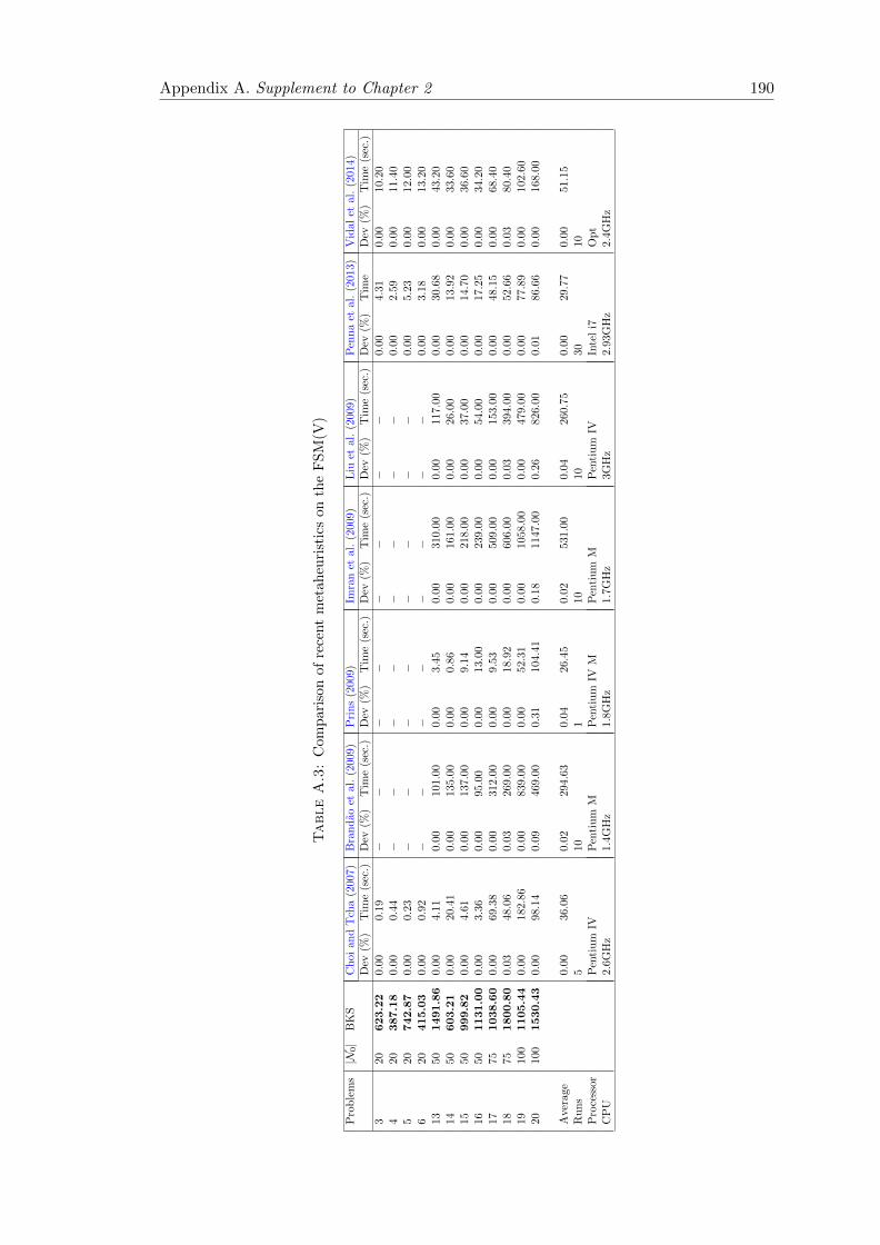
Appendix A. Supplement to Chapter 2 190
TableA.3:
Com
pari
son
of
rece
nt
met
ah
euri
stic
son
the
FS
M(V
)
Pro
ble
ms|N
0|
BK
SC
hoi
and
Tch
a(2
007)
Bra
nd
aoet
al.
(200
9)P
rin
s(2
009)
Imra
net
al.
(200
9)L
iuet
al.
(200
9)P
enn
aet
al.
(2013)
Vid
al
etal.
(2014)
Dev
(%)
Tim
e(s
ec.)
Dev
(%)
Tim
e(s
ec.)
Dev
(%)
Tim
e(s
ec.)
Dev
(%)
Tim
e(s
ec.)
Dev
(%)
Tim
e(s
ec.)
Dev
(%)
Tim
eD
ev(%
)T
ime
(sec
.)
320
623.2
20.
000.
19−
−−
−−
−−
−0.0
04.3
10.0
010.2
04
20387.1
80.
000.
44−
−−
−−
−−
−0.0
02.5
90.0
011.4
05
20742.8
70.
000.
23−
−−
−−
−−
−0.0
05.2
30.0
012.0
06
20415.0
30.
000.
92−
−−
−−
−−
−0.0
03.1
80.0
013.2
013
501491.8
60.
004.
110.
0010
1.00
0.00
3.45
0.00
310.
000.
0011
7.00
0.0
030.6
80.0
043.2
014
50603.2
10.
0020
.41
0.00
135.
000.
000.
860.
0016
1.00
0.00
26.0
00.0
013.9
20.0
033.6
015
50999.8
20.
004.
610.
0013
7.00
0.00
9.14
0.00
218.
000.
0037
.00
0.0
014.7
00.0
036.6
016
501131.0
00.
003.
360.
0095
.00
0.00
13.0
00.
0023
9.00
0.00
54.0
00.0
017.2
50.0
034.2
017
751038.6
00.
0069
.38
0.00
312.
000.
009.
530.
0050
9.00
0.00
153.
000.0
048.1
50.0
068.4
018
751800.8
00.
0348
.06
0.03
269.
000.
0018
.92
0.00
606.
000.
0339
4.00
0.0
052.6
60.0
380.4
019
100
1105.4
40.
0018
2.86
0.00
839.
000.
0052
.31
0.00
1058
.00
0.00
479.
000.0
077.8
90.0
0102.6
020
100
1530.4
30.
0098
.14
0.09
469.
000.
3110
4.41
0.18
1147
.00
0.26
826.
000.0
186.6
60.0
0168.0
0
Ave
rage
0.00
36.0
60.
0229
4.63
0.04
26.4
50.
0253
1.00
0.04
260.
750.0
029.7
70.0
051.1
5R
un
s5
101
1010
30
10
Pro
cess
orP
enti
um
IVP
enti
um
MP
enti
um
IVM
Pen
tiu
mM
Pen
tiu
mIV
Inte
li7
Op
tC
PU
2.6G
Hz
1.4G
Hz
1.8G
Hz
1.7G
Hz
3GH
z2.9
3G
Hz
2.4
GH
z
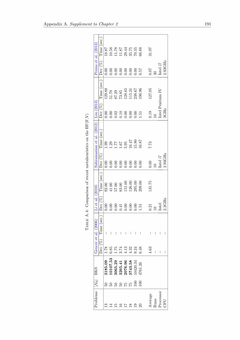
Appendix A. Supplement to Chapter 2 191
TableA.4:
Com
pari
son
of
rece
nt
met
ah
euri
stic
son
the
HF
(F,V
)
Pro
ble
ms|N
0|
BK
SG
ence
ret
al.
(200
6)L
iet
al.
(201
0)
Sub
ram
ania
net
al.
(201
2)L
iu(2
013)
Pen
na
etal
.(2
013)
Dev
(%)
Tim
e(s
ec.)
Dev
(%)
Tim
e(s
ec.)
Dev
(%)
Tim
e(s
ec.)
Dev
(%)
Tim
e(s
ec.)
Dev
(%)
Tim
e(s
ec.)
1350
3185.0
91.
78−
0.00
92.
000.0
01.
990.
0012
9.8
80.
0018
.87
1450
10107.5
30.
85−
0.00
41.
000.0
01.
290.
0051
.78
0.00
10.5
815
503065.2
91.
75−
0.00
57.
000.0
01.
770.
0287
.29
0.00
11.7
816
503265.4
13.
74−
0.41
83.
000.0
01.
670.
1073
.85
0.00
11.8
717
752076.9
64.
13−
0.00
151
.00
0.0
05.
950.
0012
8.6
50.
0029
.44
1875
3743.5
84.
32−
0.00
126
.00
0.0
016
.47
0.00
115.3
10.
0035
.75
1910
0104
20.3
49.
24−
0.00
295
.00
0.0
015
.80
0.00
238.6
70.
0070
.55
2010
0476
1.26
6.48
−1.
51
209
.00
0.0
016
.87
1.51
190.9
60.
5766
.88
Ave
rage
4.63
−0.
21
131
.75
0.0
07.
730.
1912
7.0
50.
0731
.97
Runs
−−
1010
1030
Pro
cess
or−
−In
tel
Inte
li7
Inte
lP
enti
um
IVIn
tel
i7C
PU
−−
2.2G
Hz
2.9
3GH
z3G
Hz
2.93
GH
z

Appendix A. Supplement to Chapter 2 192
TableA.5:
Com
pari
son
of
rece
nt
met
ah
euri
stic
son
the
HF
(V)
Pro
ble
ms|N
0|
BK
ST
ailla
rd(1
999)
Tar
anti
lis
etal
.(2
004
)L
iet
al.
(200
7)P
rins
(200
9)Subra
man
ian
etal
.(2
012
)L
iu(2
013)
Pen
na
etal
.(2
013
)D
ev(%
)T
ime
(sec
.)D
ev(%
)T
ime
(sec
.)D
ev(%
)T
ime
(sec
.)D
ev(%
)T
ime
(sec
.)D
ev(%
)T
ime
(sec
.)D
ev(%
)T
ime
(sec
.)D
ev(%
)T
ime
(sec
.)
13
50
1517.8
40.
0147
3.00
0.14
843.
000.
0035
8.00
0.00
33.2
00.
001.
330.0
057
.42
0.00
19.
2914
50
607.5
31.
3357
5.00
0.64
387.
000.
0014
1.00
0.00
37.6
00.
001.
090.0
086
.98
0.00
11.
2015
50
1015.2
90.
1533
5.00
0.00
368.
000.
0016
6.00
0.00
6.60
0.00
2.13
0.0
04.
850.
0012.
5616
50
1144.9
40.
8035
0.00
0.05
341.
000.
0018
8.00
0.00
7.50
0.00
1.41
0.0
013
.51
0.00
12.
2917
75
1061.9
60.
9322
45.0
00.
85
363.
000.
0021
6.00
0.20
81.5
00.
004.
220.0
011
5.88
0.00
29.
9218
75
1823.5
82.
5528
76.0
01.
25
971.
000.
0036
6.00
0.00
190.
600.
004.
060.0
097
.98
0.00
38.
3419
100
1117
.51
2.55
5833
.00
0.57
428.
000.
2540
4.00
0.25
177.
800.
259.
120.2
577
.21
0.25
67.
7220
100
1534.1
71.
6734
02.0
00.
57
1156
.00
0.00
447.
000.
0022
3.30
0.00
8.89
0.0
011
5.49
0.00
63.
77
Ave
rage
1.25
2011
.13
0.51
607.
130.
0328
5.75
0.06
94.7
60.
034.
030.0
371
.17
0.03
31.
89R
uns
51
11
1010
30P
roce
ssor
Sun
Sparc
Pen
tium
IIA
MD
Ath
lon
Pen
tium
IVM
Inte
li7
Inte
lP
enti
um
IVIn
tel
i7C
PU
50M
Hz
400M
Hz
1.0G
Hz
1.8G
Hz
2.93
GH
z3G
Hz
2.93
GH
z

Appendix B
Supplement to Chapter 3
Table B.1 shows the four versions of the HEA. Table B.2 presents the best results of ten
runs for each of four versions. Table B.3 shows the number of times for each removal and
insertion operators was called within the HEA. Tables B.4 to B.9 present the detailed
results on all benchmark instances for FT and FD.
193

Appendix B. Supplement to Chapter 3 194
Table B.1: Sensitivity analyis experiment setup
Version Education Intensification Diversification
1 No No No2 Yes No No3 Yes Yes NoHEA Yes Yes Yes
Table B.2: Sensitivity analyis of the HEA components
Instance Version (1) Version (2) Version (3) HEATC Dev Time TC Dev Time TC Dev Time TC Time
C101A 7271.60 0.62 2.79 7259.60 0.46 2.85 7246.51 0.28 2.91 7226.51 2.97C203A 5795.12 0.93 4.53 5781.12 0.69 4.61 5761.12 0.35 4.69 5741.12 4.76R101A 4591.80 1.09 4.49 4580.80 0.85 4.58 4571.70 0.66 5.09 4541.70 5.26R211A 3061.11 1.32 7.72 3050.11 0.97 7.81 3040.56 0.66 7.87 3020.56 7.99RC105A 5146.19 0.55 5.14 5136.19 0.35 5.21 5128.19 0.20 5.27 5118.10 5.32RC207A 4362.19 1.08 5.59 4351.19 0.83 6.11 4335.19 0.46 6.21 4315.19 6.27Avg 0.93 5.04 0.69 5.20 0.43 5.34 5.43
Table B.3: Number of iterations as a percentage by education operators
Instance Removal operators Insertion operatorsRR WDR WTR NR SR PBR TBR DR ACUTR GI GINF
C101A 6.30 13.70 12.80 14.30 14.20 7.20 8.60 7.20 15.70 65.20 34.80C203A 6.10 13.90 12.40 14.50 14.00 7.90 9.00 7.00 15.20 60.80 39.20R101A 6.90 12.50 13.60 14.80 13.90 7.90 8.00 7.00 15.40 71.20 28.80R211A 6.30 13.50 12.80 14.50 14.20 6.70 8.60 7.90 15.50 67.80 32.20RC105A 5.30 14.70 11.80 13.50 15.20 8.90 7.70 7.60 15.30 69.10 30.90RC207A 7.40 12.60 14.50 13.60 12.90 8.20 7.10 7.90 15.80 66.40 33.60Avg 6.38 13.48 12.98 14.20 14.07 7.80 8.17 7.43 15.48 66.75 33.25
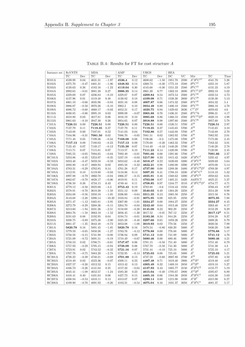
Appendix B. Supplement to Chapter 3 195
Table B.4: Results for FT for cost structure A
Instance set ReVNTS MDA AMP UHGS HEATC Dev TC Dev TC Dev TC Dev DC VC Mix TC Time
R101A 4539.99 0.04 4631.31 −1.97 4536.4 0.12 4608.62 −1.50 1951.70 2590 A1B2C17 4541.70 5.26R102A 4375.70 −0.47 4401.31 −1.06 4348.92 0.14 4369.74 −0.30 1775.10 2580 B6C15 4355.10 5.87R103A 4120.63 0.26 4182.16 −1.23 4119.04 0.30 4145.68 −0.30 1551.23 2580 B6C15 4131.23 4.19R104A 3992.65 −0.01 3981.28 0.27 3986.35 0.14 3961.39 0.77 1302.10 2690 B5C11D3 3992.10 5.02R105A 4229.69 0.07 4236.84 −0.10 4229.67 0.07 4209.84 0.54 1672.54 2560 B4C16 4232.54 4.73R106A 4137.96 0.01 4118.48 0.48 4130.82 0.18 4109.08 0.71 1538.30 2600 B1C18 4138.30 5.13R107A 4061.10 −0.66 4035.96 −0.04 4031.16 0.08 4007.87 0.66 1474.32 2560 B4C16 4034.32 5.4R108A 3986.07 −0.50 3970.26 −0.10 3962.2 0.10 3934.48 0.80 1406.10 2560 B4C16 3966.10 4.78R109A 4086.72 −0.68 4060.17 −0.03 4052.21 0.17 4020.75 0.94 1429.02 2630 C17D1 4059.02 4.6R110A 4030.85 −0.86 3995.18 0.03 3999.09 −0.07 3965.88 0.76 1436.31 2560 B4C16 3996.31 4.17R111A 4018.80 0.03 4017.81 0.06 4016.19 0.10 3985.68 0.86 1460.10 2560 B4C13D2 4020.10 4.98R112A 3961.63 −0.10 3947.30 0.26 3954.65 0.07 3918.88 0.98 1397.60 2560 B4C16 3957.60 5.78C101A 7226.51 0.00 7226.51 0.00 7226.51 0.00 7226.51 0.00 1526.51 5700 A19 7226.51 2.97C102A 7137.79 0.11 7119.35 0.37 7137.79 0.11 7119.35 0.37 1445.65 5700 A19 7145.65 3.10C103A 7143.88 0.00 7107.01 0.52 7141.03 0.04 7102.86 0.57 1443.88 5700 A19 7143.88 2.70C104A 7104.96 −0.31 7081.50 0.02 7086.70 −0.05 7081.51 0.02 1382.92 5700 A19 7082.92 2.01C105A 7171.48 0.05 7199.36 −0.34 7169.08 0.08 7196.06 −0.3 1475.00 5700 A19 7175.00 2.45C106A 7157.13 0.09 7180.03 −0.23 7157.13 0.09 7176.68 −0.20 1463.32 5700 A19 7163.32 3.01C107A 7135.43 0.07 7149.17 −0.13 7135.38 0.07 7144.49 −0.10 1440.20 5700 A19 7140.20 2.78C108A 7115.71 0.07 7115.81 0.07 7113.57 0.10 7111.23 0.14 1420.98 5700 A19 7120.98 2.45C109A 7095.55 −0.05 7094.65 −0.04 7092.49 −0.01 7091.66 0.00 1391.66 5700 A19 7091.66 2.37RC101A 5253.86 −0.35 5253.97 −0.35 5237.19 −0.03 5217.90 0.33 1815.42 3420 A2B8C7 5235.42 4.97RC102A 5053.48 −0.47 5059.58 −0.59 5053.62 −0.48 5018.47 0.22 1639.69 3390 A4B3C9 5029.69 5.64RC103A 4892.80 −0.47 4868.94 0.02 4885.58 −0.32 4822.21 0.98 1480.00 3390 A4B3C9 4870.00 5.14RC104A 4783.31 −0.29 4762.85 0.14 4761.28 0.17 4737.00 0.68 1289.30 3480 A3B1C9D1 4769.30 4.97RC105A 5112.91 0.10 5119.80 −0.03 5110.86 0.14 5097.35 0.41 1788.10 3330 A3B11C5 5118.10 5.32RC106A 4997.98 −0.79 4960.78 −0.04 4966.27 −0.15 4935.91 0.46 1568.62 3390 A4B9C6 4958.62 6.01RC107A 4862.67 −0.78 4828.17 −0.06 4819.91 0.11 4783.08 0.87 1405.21 3420 A4B7C7 4825.21 5.37RC108A 4736.50 0.38 4734.15 0.43 4749.44 0.11 4708.85 0.97 1244.77 3510 A1B2C9D1 4754.77 4.71R201A 3779.12 −0.50 3922.00 −4.3 3753.42 0.19 3782.88 −0.6 1510.43 2250 A5 3760.43 8.97R202A 3578.91 −0.70 3610.38 −1.58 3551.12 0.09 3540.03 0.40 1304.20 2250 A5 3554.20 9.98R203A 3334.08 −0.56 3350.18 −1.05 3336.60 −0.64 3311.35 0.13 1065.50 2250 A5 3315.50 8.76R204A 3143.68 −2.20 3390.14 −10.20 3103.84 −0.91 3075.95 0.00 825.95 2250 A5 3075.95 7.98R205A 3371.47 −1.12 3465.81 −3.95 3367.90 −1.01 3334.27 0.00 1084.27 2250 A5 3334.27 8.45R206A 3272.79 −0.29 3268.36 −0.15 3264.70 −0.04 3242.40 0.64 1013.40 2250 A5 3263.40 8.17R207A 3213.60 −1.94 3231.26 −2.51 3158.69 −0.20 3145.08 0.23 902.29 2250 A5 3152.29 9.29R208A 3064.76 −1.58 3063.10 −1.52 3056.45 −1.30 3017.52 −0.01 767.12 2250 A5 3017.12* 8.51R209A 3191.63 0.08 3192.95 0.04 3194.74 −0.01 3183.36 0.34 944.28 2250 A5 3194.28 9.37R210A 3338.75 −0.89 3375.38 −2.00 3325.28 −0.48 3287.66 0.65 1059.26 2250 A5 3309.26 8.79R211A 3061.47 −1.35 3042.48 −0.73 3053.08 −1.08 3019.93 0.02 770.56 2250 A5 3020.56 7.99C201A 5820.78 0.16 5891.45 −1.05 5820.78 0.16 5878.54 −0.80 830.20 5000 A5 5830.20 5.00C202A 5779.59 −0.05 5850.26 −1.27 5783.76 −0.12 5776.88 0.00 776.88 5000 A5 5776.88 5.17C203A 5750.58 −0.15 5741.90 −0.00 5736.94 0.09 5741.12 0.00 741.89 5000 A5 5741.12 4.76C204A 5721.09 −0.72 5691.51 −0.19 5718.49 −0.67 5680.46 0.00 680.46 5000 A5 5680.46 4.21C205A 5750.53 0.02 5786.71 −0.61 5747.67 0.06 5781.15 −0.50 751.40 5000 A5 5751.40 6.79C206A 5757.93 −0.29 5795.15 −0.94 5738.09 0.06 5767.70 −0.50 741.30 5000 A5 5741.30 4.3C207A 5723.91 0.02 5743.52 −0.32 5721.16 0.07 5731.44 −0.10 725.10 5000 A5 5725.10 4.17C208A 5767.78 −0.75 5884.20 −2.78 5732.95 −0.14 5725.03 0.00 725.03 5000 A5 5725.03 5.21RC201A 4726.22 −0.39 4740.21 −0.69 4701.88 0.13 4737.59 −0.60 2007.80 2700 A18 4707.80 4.50RC202A 4518.49 0.02 4522.36 −0.07 4509.11 0.23 4487.48 0.71 1619.40 2900 A10B4 4519.40 4.67RC203A 4327.57 −0.20 4312.52 0.15 4313.42 0.13 4305.49 0.32 1469.10 2850 A12B3 4319.10 5.27RC204A 4166.73 −0.26 4141.04 0.35 4157.32 −0.04 4137.93 0.43 1005.77 3150 A2B5C2 4155.77 5.19RC205A 4645.41 −1.08 4652.57 −1.24 4585.20 0.23 4615.04 −0.40 1795.67 2800 A14B2 4595.67 6.89RC206A 4416.41 0.40 4431.64 0.06 4427.73 0.15 4405.16 0.66 1584.30 2850 A9B3C1 4434.30 5.03RC207A 4338.94 −0.53 4310.11 0.13 4313.07 0.07 4290.14 0.60 1215.90 3100 A4B7 4315.90 6.27RC208A 4109.90 −0.70 4091.92 −0.26 4103.31 −0.54 4075.04 0.16 1031.37 3050 A5B5C1 4081.37 5.17
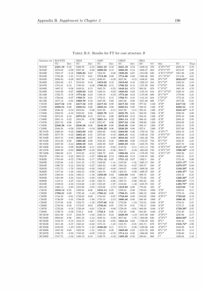
Appendix B. Supplement to Chapter 3 196
Table B.5: Results for FT for cost structure B
Instance set ReVNTS MDA AMP UHGS HEATC Dev TC Dev TC Dev TC Dev DC VC Mix TC Time
R101B 2421.19 0.16 2486.76 −2.54 2421.19 0.16 2421.19 0.16 1849.10 576 A1B4C9D5 2425.10 3.78R102B 2219.03 −0.30 2227.48 −0.68 2209.50 0.13 2209.50 0.13 1608.37 604 A2B1C6D8 2212.37 3.97R103B 1955.57 −0.18 1938.93 0.67 1953.50 −0.08 1938.93 0.67 1313.99 638 A1B1C4D6E2 1951.99 4.28R104B 1732.26 −1.01 1714.73 0.01 1713.36 0.09 1713.36 0.09 1026.86 688 A1C1D5E4 1714.86 4.01R105B 2030.83 −0.29 2027.98 −0.15 2030.83 −0.29 2027.98 −0.15 1436.91 588 B3C5D8 2024.91* 3.68R106B 1924.03 −0.1 1919.03 0.16 1919.02 0.16 1919.02 0.16 1338.10 584 B1C6D8 1922.10 4.19R107B 1781.01 0.12 1789.58 −0.36 1780.52 0.15 1780.52 0.15 1127.20 656 C2D8E2 1783.20 5.30R108B 1667.51 −0.36 1649.24 0.74 1665.78 −0.25 1649.24 0.74 983.58 678 C1D5E4 1661.58 4.78R109B 1844.99 −0.87 1828.63 0.03 1840.54 −0.63 1828.63 0.03 1185.10 644 B1C1D10E1 1829.10 4.91R110B 1792.75 −0.78 1774.46 0.24 1788.18 −0.53 1774.46 0.24 1178.80 600 B1C3D10 1778.80 5.21R111B 1780.03 −0.27 1769.71 0.31 1772.51 0.15 1769.71 0.31 1141.24 634 C3D7E2 1775.24 4.78R112B 1677.13 −0.01 1669.78 0.43 1667.00 0.60 1667.00 0.60 1071.00 606 C2D11 1677.00 6.21C101B 2417.52 0.00 2417.52 0.00 2417.52 0.00 2417.52 0.00 977.52 1440 A8B6 2417.52 1.99C102B 2350.54 0.00 2350.54 0.00 2350.54 0.00 2350.54 0.00 930.54 1420 A5B7 2350.54 2.45C103B 2349.42 −0.18 2353.64 −0.36 2347.99 −0.11 2347.99 −0.11 925.31 1420 A5B7 2345.31* 3.47C104B 2332.94 −0.10 2328.62 0.08 2325.78 0.21 2325.78 0.21 950.59 1380 A7B6 2330.59 3.09C105B 2374.01 0.10 2373.53 0.12 2375.04 0.06 2373.53 0.12 956.45 1420 A5B7 2376.45 3.06C106B 2381.14 0.22 2404.56 −0.76 2381.14 0.22 2381.14 0.22 966.43 1420 A5B7 2386.43 2.95C107B 2357.52 0.06 2370 −0.47 2357.67 0.06 2357.52 0.06 939.00 1420 A5B7 2359.00 2.45C108B 2346.38 0.08 2346.38 0.08 2346.38 0.08 2346.38 0.08 968.15 1380 A7B6 2348.15 2.79C109B 2346.58 −0.38 2339.89 −0.10 2336.29 0.06 2336.29 0.06 957.6 1380 A7B6 2337.60 2.56RC101B 2469.50 −0.22 2462.60 0.06 2464.66 −0.02 2462.60 0.06 1732.19 732 A1B4C10 2464.19 4.47RC102B 2277.79 −0.32 2263.45 0.31 2272.68 −0.10 2263.45 0.31 1538.43 732 A1B3C9D1 2270.43 4.12RC103B 2057.55 −0.80 2035.62 0.27 2041.24 −0.00 2035.62 0.27 1291.20 750 B1C9D2 2041.20 3.98RC104B 1914.93 0.38 1905.06 0.90 1916.85 0.28 1905.06 0.90 1172.27 750 B1C6D4 1922.27 4.21RC105B 2337.93 −0.44 2308.59 0.82 2325.99 0.07 2308.59 0.82 1625.70 702 A1B7C8 2327.70 4.56RC106B 2168.44 −0.99 2149.56 −0.11 2160.45 −0.62 2149.56 −0.11 1415.14 732 A1B2C8D2 2147.14* 4.21RC107B 2008.39 −0.62 2000.77 −0.23 2003.26 −0.36 2000.77 −0.23 1264.09 732 A1B2C5D4 1996.09* 4.19RC108B 1906.69 0.12 1910.83 −0.10 1908.72 0.01 1906.69 0.12 1176.89 732 A1B1C7D3 1908.89 3.11R201B 1965.10 −0.45 2002.53 −2.37 1953.42 0.14 1953.42 0.14 1456.21 500 A4B1 1956.21 6.21R202B 1765.09 −0.72 1790.38 −2.17 1751.12 0.07 1751.12 0.07 1302.4 450 A5 1752.40 8.00R203B 1535.08 −1.31 1541.19 −1.72 1536.60 −1.41 1535.08 −1.31 1065.17 450 A5 1515.17* 5.78R204B 1306.72 −2.12 1284.33 −0.37 1303.84 −1.90 1284.33 −0.37 829.57 450 A5 1279.57* 6.89R205B 1575.75 −1.70 1563.62 −0.92 1560.07 −0.69 1560.07 −0.69 1099.39 450 A5 1549.39* 6.49R206B 1477.34 −1.86 1464.53 −0.98 1464.70 −0.99 1464.53 −0.98 1000.37 450 A5 1450.37* 5.21R207B 1386.84 −2.04 1380.41 −1.56 1358.69 0.04 1358.69 0.04 909.18 450 A5 1359.18 6.31R208B 1261.09 −3.34 1244.74 −2.00 1256.45 −2.96 1244.74 −2.00 770.36 450 A5 1220.36* 5.47R209B 1418.51 −2.37 1431.37 −3.30 1394.74 −0.66 1394.74 −0.66 935.65 450 A5 1385.65* 7.14R210B 1529.04 −2.23 1516.66 −1.40 1525.28 −1.97 1516.66 −1.40 1045.75 450 A5 1495.75* 6.93R211B 1268.14 −3.95 1255.06 −2.88 1253.08 −2.72 1219.93 0.00 770.56 450 A5 1219.93 7.45C201B 1816.14 0.25 1820.64 0.00 1816.14 0.25 1820.64 0.00 740.64 1080 A4B1 1820.64 3.11C202B 1768.51 0.09 1795.40 −1.43 1768.51 0.09 1768.51 0.09 690.10 1080 A2B1C1 1770.10 4.58C203B 1744.28 −0.61 1733.63 0.00 1734.82 −0.07 1733.63 0.00 653.63 1080 A2B1C1 1733.63 3.19C204B 1736.09 −3.31 1708.69 −1.68 1716.18 −2.13 1680.46 0.00 680.46 1000 A5 1680.46 3.17C205B 1747.68 0.50 1782.74 −1.49 1747.68 0.50 1778.30 −1.24 716.54 1040 A1B3 1756.54 5.21C206B 1756.93 0.92 1772.87 0.02 1756.01 0.97 1767.70 0.31 733.17 1040 A1B3 1773.17 3.46C207B 1732.20 −0.16 1729.49 −0.01 1729.39 −0.00 1729.49 −0.01 689.39 1040 A1B3 1729.39* 2.97C208B 1730.72 −0.38 1724.2 0.00 1723.2 0.06 1724.20 0.00 684.20 1040 A1B3 1724.20 3.13RC201B 2231.69 0.19 2343.79 −4.83 2230.54 0.24 2329.59 −4.19 1615.90 620 A4B4C2 2235.90 4.17RC202B 2002.62 0.96 2091.53 −3.44 2022.54 −0.03 2057.66 −1.76 1392.00 630 A3B3C3 2022.00* 5.47RC203B 1843.72 −0.18 1852.74 −0.67 1841.26 −0.05 1824.54 0.86 1190.40 650 B3C4 1840.40 5.12RC204B 1611.28 −3.57 1565.31 −0.62 1575.18 −1.25 1555.75 −0.01 885.74 670 B1C4D1 1555.74* 4.98RC205B 2195.62 −1.23 2195.75 −1.23 2166.62 0.11 2174.74 −0.26 1529.00 640 A2B2C4 2169.00 6.47RC206B 1887.23 0.60 1923.56 −1.31 1893.13 0.29 1883.08 0.82 1218.70 680 B5C1D1 1898.70 4.14RC207B 1780.72 −2.93 1745.85 −0.92 1743.23 −0.76 1714.14 0.92 1080.00 650 B3C4 1730.00 5.14RC208B 1557.74 −4.50 1488.19 0.16 1526.78 −2.42 1483.20 0.50 830.64 660 C6 1490.64 4.43

Appendix B. Supplement to Chapter 3 197
Table B.6: Results for FT for cost structure C
Instance set ReVNTS MDA AMP UHGS HEATC Dev TC Dev TC Dev TC Dev DC VC Mix TC Time
R101C 2134.90 0.11 2199.78 −2.93 2134.90 0.11 2199.79 −2.93 1840.20 297 A1B2C9D6 2137.20 3.14R102C 1913.37 0.08 1925.55 −0.56 1913.37 0.08 1925.56 −0.56 1599.87 315 A2B3C4D7E1 1914.87 6.21R103C 1633.62 −0.77 1609.94 0.69 1631.47 −0.63 1615.38 0.36 1310.20 311 A1C4D8E1 1621.20 3.24R104C 1382.82 −0.52 1370.84 0.35 1377.81 −0.16 1363.26 0.90 1025.60 350 D8E3 1375.60 4.47R105C 1729.57 −0.44 1722.05 0.00 1729.57 −0.44 1722.05 0.00 1403.05 319 B2C2D11 1722.05 3.17R106C 1607.96 0.15 1602.87 0.47 1607.96 0.15 1599.04 0.71 1285.40 325 A1C5D6E2 1610.40 4.08R107C 1455.09 −0.05 1456.02 −0.12 1452.52 0.12 1442.97 0.78 1126.30 328 C2D8E2 1454.30 3.51R108C 1331.54 −0.12 1336.28 −0.48 1330.28 −0.03 1321.68 0.62 979.92 350 D6E4 1329.92 5.33R109C 1525.65 −1.23 1507.77 −0.04 1519.37 −0.81 1505.59 0.10 1185.10 322 B1C1D10E1 1507.10 4.73R110C 1463.91 −0.89 1446.41 0.32 1457.43 −0.44 1443.92 0.49 1109.06 342 C3D4E4 1451.06 5.46R111C 1451.92 −1.09 1447.88 −0.80 1443.34 −0.49 1423.47 0.89 1098.32 338 B1D9E2 1436.32 6.14R112C 1355.78 −1.09 1335.41 0.42 1339.44 0.12 1329.07 0.90 988.10 353 C2D5E4 1341.10 4.17C101C 1628.94 0.00 1628.31 0.04 1628.94 0.00 1628.94 0.00 828.94 800 B10 1628.94 1.97C102C 1610.96 0.00 1610.96 0.00 1610.96 0.00 1610.96 0.00 860.96 750 A1B9 1610.96 2.53C103C 1611.14 −0.25 1619.68 −0.78 1607.14 0.00 1607.14 0.00 857.14 750 A1B9 1607.14 3.79C104C 1610.07 −0.68 1613.96 −0.92 1598.50 0.04 1599.90 −0.04 869.21 730 A3B8 1599.21 2.89C105C 1628.94 0.00 1628.38 0.03 1628.94 0.00 1628.94 0.00 828.94 800 B10 1628.94 1.97C106C 1628.94 0.00 1628.94 0.00 1628.94 0.00 1628.94 0.00 828.94 800 B10 1628.94 2.01C107C 1628.94 0.00 1628.38 0.03 1628.94 0.00 1628.94 0.00 828.94 800 B10 1628.94 1.99C108C 1622.89 0.13 1622.89 0.13 1622.89 0.13 1622.89 0.13 825 800 B10 1625.00 2.45C109C 1619.02 −0.03 1614.99 0.22 1614.99 0.22 1615.93 0.17 888.61 730 A3B8 1618.61 3.54RC101C 2089.37 0.13 2084.48 0.36 2089.37 0.13 2082.95 0.44 1702.10 390 B7C5D3 2092.10 4.54RC102C 1918.96 −0.90 1895.92 0.31 1906.68 −0.25 1895.05 0.36 1529.89 372 A2B2C8D2 1901.89 4.19RC103C 1674.50 −0.83 1660.62 0.00 1666.24 −0.33 1650.30 0.63 1300.7 360 C12 1660.70 3.56RC104C 1543.55 −0.19 1537.09 0.23 1540.13 0.03 1526.04 0.95 1159.60 381 A1C5D5 1540.60 3.47RC105C 1972.57 −0.84 1957.52 −0.07 1953.99 0.11 1957.14 −0.05 1584.09 372 A2B2C8D2 1956.09 4.16RC106C 1793.12 −0.71 1776.08 0.25 1787.69 −0.41 1774.94 0.31 1393.45 387 A2B1C6D4 1780.45 3.49RC107C 1635.65 −0.95 1614.04 0.39 1622.90 −0.16 1607.11 0.81 1245.30 375 B3C5D4 1620.30 3.07RC108C 1531.69 0.06 1535.14 −0.17 1531.69 0.06 1523.96 0.56 1157.60 375 B2C6D4 1532.60 3.56R201C 1745.39 −0.82 1729.92 0.07 1728.42 0.16 1716.02 0.88 1461.20 270 A6 1731.20 6.78R202C 1537.33 −0.50 1537.35 −0.50 1527.92 0.12 1515.96 0.90 1304.70 225 A5 1529.70 8.14R203C 1338.42 −3.22 1308.70 −0.92 1311.60 −1.15 1286.35 0.80 1071.72 225 A5 1296.72 6.50R204C 1080.66 −2.64 1062.46 −0.91 1085.71 −3.12 1050.95 0.19 802.90 250 A5 1052.90 7.89R205C 1350.12 −2.66 1311.84 0.26 1335.07 −1.51 1309.27 0.45 1090.20 225 A5 1315.20 6.71R206C 1254.67 −2.26 1251.51 −2.00 1239.70 −1.04 1216.35 0.86 1001.93 225 A5 1226.93 6.59R207C 1186.05 −5.38 1149.23 −2.11 1139.61 −1.25 1120.08 0.48 900.50 225 A5 1125.50 6.98R208C 1022.31 −2.44 1009.26 −1.13 1022.11 −2.42 992.12 0.59 772.97 225 A5 997.97 5.87R209C 1233.07 −5.91 1178.45 −1.21 1171.41 −0.61 1155.79 0.73 939.31 225 A4B1 1164.31 7.14R210C 1284.72 −1.18 1289.35 −1.55 1281.08 −0.90 1257.89 0.93 1019.70 250 A4B1 1269.70 6.14R211C 1061.70 −6.64 1013.84 −1.83 1028.08 −3.26 994.93 0.07 770.58 225 A5 995.58 6.17C201C 1269.41 −1.47 1269.41 −1.47 1269.41 −1.47 1269.41 −1.47 650.97 600 A2C2 1250.97* 2.97C202C 1252.24 −0.92 1242.66 −0.15 1244.54 −0.30 1239.54 0.11 700.86 540 A2B1C1 1240.86 3.54C203C 1228.13 −2.89 1193.63 0.00 1203.42 −0.82 1193.63 0.00 653.63 540 A2B1C1 1193.63 3.14C204C 1207.03 −2.59 1176.52 0.00 1188.18 −0.99 1176.52 0.00 636.52 540 A2B1C1 1176.52 3.67C205C 1245.51 −0.44 1245.62 −0.45 1239.60 0.04 1238.30 0.15 640.1 600 A2B2 1240.10 4.29C206C 1229.63 −0.03 1245.05 −1.29 1229.23 0.00 1238.30 −0.74 629.23 600 A2C2 1229.23 4.38C207C 1221.16 −0.97 1215.42 −0.49 1213.07 −0.30 1209.49 −0.01 689.48 520 A2B1C1 1209.48* 3.56C208C 1210.72 −0.54 1204.20 0.00 1205.18 −0.08 1204.20 0.00 684.2 520 A1B3 1204.20 3.01RC201C 1957.60 −2.07 2004.53 −4.52 1915.42 0.13 1996.79 −4.11 1577.90 340 A3B3C2D1 1917.90 4.65RC202C 1699.48 −1.16 1766.52 −5.15 1677.62 0.14 1732.66 −3.13 1355.00 325 A1B5C1D1 1680.00 6.10RC203C 1510.13 −0.66 1517.98 −1.19 1504.35 −0.28 1496.11 0.27 1160.20 340 A2B1C3E1 1500.20 6.27RC204C 1256.91 −2.84 1238.66 −1.35 1241.45 −1.58 1220.75 0.12 887.16 335 B1C4E1 1222.16 5.47RC205C 1901.71 −4.32 1854.22 −1.71 1822.07 0.05 1844.74 −1.19 1453 370 B2C4D1 1823.00 5.29RC206C 1598.84 −2.21 1590.22 −1.66 1586.61 −1.43 1553.65 0.68 1224.3 340 B5C1E1 1564.30 4.70RC207C 1431.65 −3.61 1396.16 −1.05 1406.26 −1.78 1377.52 0.30 1026.71 355 C3D1E1 1381.71 5.67RC208C 1181.47 −2.61 1145.84 0.48 1175.23 −2.07 1140.10 0.98 821.40 330 C6 1151.40 5.17

Appendix B. Supplement to Chapter 3 198
Table B.7: Results for FD for cost structure A
Instance set MDA BPDRT UHGS HEATC Dev TC Dev TC Dev DC VC Mix TC Time
R101A 4349.80 −0.75 4342.72 −0.58 4314.36 0.07 1787.52 2530 A1B10C12 4317.52 4.14R102A 4196.46 −0.54 4189.21 −0.37 4166.28 0.18 1623.84 2550 A1B5C15 4173.84 5.98R103A 4052.85 −0.53 4051.62 −0.50 4027.36 0.10 1401.40 2630 B1C18 4031.40 5.21R104A 3978.48 −0.81 3972.65 −0.66 3936.40 0.25 1276.44 2670 B3C15D1 3946.44 4.12R105A 4161.72 −0.67 4152.50 −0.45 4122.50 0.28 1574.06 2560 A1B5C15 4134.06 6.01R106A 4095.20 −0.87 4085.30 −0.62 4048.59 0.28 1500.05 2560 B4C16 4060.05 5.12R107A 4006.61 −0.54 3996.74 −0.29 3970.51 0.37 1395.12 2590 B3C15D1 3985.12 4.78R108A 3961.38 −0.73 3949.50 −0.43 3928.12 0.11 1342.60 2590 B3C15D1 3932.60 6.54R109A 4048.29 −0.58 4035.89 −0.27 4015.71 0.23 1464.83 2560 B4C16 4024.83 6.12R110A 3997.88 −0.61 3991.63 −0.46 3961.68 0.30 1373.51 2600 B1C18 3973.51 5.21R111A 4011.63 −0.59 4009.61 −0.54 3964.99 0.58 1368.00 2620 B3C15D1 3988.00 5.12R112A 3962.73 −0.83 3954.19 −0.61 3918.88 0.29 1300.19 2630 C17D1 3930.19 4.71C101A 7098.04 −0.06 7097.93 −0.06 7093.45 0.00 1393.45 5700 A19 7093.45 2.47C102A 7086.11 −0.08 7085.47 −0.07 7080.17 0.00 1380.17 5700 A19 7080.17 2.65C103A 7080.35 −0.02 7080.41 −0.02 7079.21 0.00 1379.21 5700 A19 7079.21 2.01C104A 7076.90 −0.03 7075.06 0.00 7075.06 0.00 1375.06 5700 A19 7075.06 1.97C105A 7096.19 −0.04 7096.22 −0.04 7093.45 0.00 1393.45 5700 A19 7093.45 2.65C106A 7086.91 −0.04 7088.35 −0.06 7083.87 0.00 1383.87 5700 A19 7083.87 2.17C107A 7084.92 −0.00 7090.91 −0.09 7084.61 0.00 1384.61 5700 A19 7084.61 2.39C108A 7082.49 −0.04 7081.18 −0.02 7079.66 0.00 1379.66 5700 A19 7079.66 1.97C109A 7078.13 −0.01 7077.68 −0.01 7077.30 0.00 1377.30 5700 A19 7077.30 2.19RC101A 5180.74 −0.14 5168.23 0.10 5150.86 0.44 1843.47 3330 A3B13C4 5173.47 5.14RC102A 5029.59 −0.21 5025.22 −0.13 4987.24 0.63 1658.83 3360 A6B6C7 5018.83 4.26RC103A 4895.57 −0.94 4888.53 −0.79 4804.61 0.94 1430.20 3420 A2B6C8 4850.20 6.47RC104A 4760.56 −0.74 4747.38 −0.47 4717.63 0.16 1395.40 3330 A3B2C8D1 4725.40 5.29RC105A 5060.37 −0.23 5068.54 −0.39 5035.35 0.27 1748.86 3300 A5B8C6 5048.86 4.78RC106A 4997.86 −0.68 4972.11 −0.16 4936.74 0.55 1514.13 3450 B7C8 4964.13 5.29RC107A 4865.76 −0.83 4861.04 −0.73 4788.69 0.76 1435.60 3390 A4B5C8 4825.60 4.17RC108A 4765.37 −0.86 4753.12 −0.60 4708.85 0.34 1334.79 3390 A4B2C8D1 4724.79 4.63R201A 3484.95 −1.11 3530.24 −2.42 3446.78 0.00 1196.78 2250 A5 3446.78 6.13R202A 3335.95 −1.17 3335.61 −1.16 3308.16 −0.33 1047.42 2250 A5 3297.42* 7.46R203A 3173.95 −1.05 3164.03 −0.73 3141.09 0.00 891.09 2250 A5 3141.09 6.14R204A 3065.15 −1.56 3029.83 −0.39 3018.14 0.00 768.14 2250 A5 3018.14 6.28R205A 3277.69 −1.82 3261.19 −1.31 3218.97 0.00 968.97 2250 A5 3218.97 6.38R206A 3173.30 −0.86 3165.85 −0.62 3146.34 0.00 896.34 2250 A5 3146.34 8.14R207A 3136.47 −1.92 3102.79 −0.83 3077.58 −0.01 827.36 2250 A5 3077.36* 6.47R208A 3050.00 −1.76 3009.13 −0.40 2997.24 0.00 747.25 2250 A5 2997.25 6.34R209A 3155.73 −1.16 3155.60 −1.16 3122.42 −0.09 869.56 2250 A5 3119.56* 4.99R210A 3219.23 −1.54 3206.23 −1.13 3174.85 −0.14 920.41 2250 A5 3170.41* 5.47R211A 3055.04 −1.16 3026.02 −0.20 3019.93 0.00 769.93 2250 A5 3019.93 7.93C201A 5701.45 −0.11 5700.87 −0.10 5695.02 0.00 695.02 5000 A5 5695.02 3.46C202A 5689.70 −0.08 5689.70 −0.08 5685.24 0.00 685.24 5000 A5 5685.24 3.17C203A 5685.82 −0.08 5681.55 0.00 5681.55 0.00 681.55 5000 A5 5681.55 4.29C204A 5690.30 −0.22 5677.69 0.00 5677.66 0.00 677.67 5000 A5 5677.66 3.97C205A 5691.70 −0.01 5691.70 −0.01 5691.36 0.00 691.36 5000 A5 5691.36 3.46C206A 5691.70 −0.04 5691.70 −0.04 5689.32 0.00 689.32 5000 A5 5689.32 2.97C207A 5689.82 −0.04 5692.36 −0.09 5687.35 0.00 687.35 5000 A5 5687.35 4.10C208A 5686.50 0.00 5689.59 −0.05 5686.50 0.00 686.50 5000 A5 5686.50 3.56RC201A 4407.68 −0.71 4404.07 −0.62 4374.09 0.06 1476.82 2900 A10B4 4376.82 5.14RC202A 4277.67 −0.78 4266.96 −0.53 4244.63 0.00 1294.63 2950 A8B5 4244.63 4.26RC203A 4204.85 −0.83 4189.94 −0.47 4170.17 0.00 1120.17 3050 A6B3C2 4170.17 6.14RC204A 4109.86 −0.56 4098.34 −0.27 4087.11 0.00 937.112 3150 A5B2C3 4087.11 5.47RC205A 4329.96 −0.84 4304.52 −0.25 4291.93 0.04 1343.73 2950 A8B5 4293.73 4.19RC206A 4272.08 −0.48 4272.82 −0.49 4251.88 0.00 1251.88 3000 A6B6 4251.88 4.27RC207A 4232.81 −1.20 4219.52 −0.89 4185.98 −0.08 1182.44 3000 A6B6 4182.44* 5.64RC208A 4095.71 −0.51 4093.83 −0.46 4075.04 0.00 975.04 3100 A4B4C2 4075.04 5.31
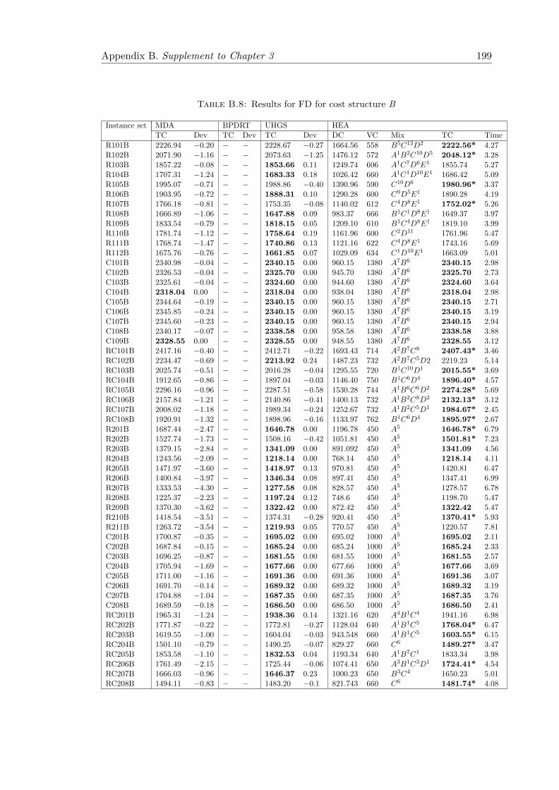
Appendix B. Supplement to Chapter 3 199
Table B.8: Results for FD for cost structure B
Instance set MDA BPDRT UHGS HEATC Dev TC Dev TC Dev DC VC Mix TC Time
R101B 2226.94 −0.20 − − 2228.67 −0.27 1664.56 558 B5C13D2 2222.56* 4.27R102B 2071.90 −1.16 − − 2073.63 −1.25 1476.12 572 A1B2C10D5 2048.12* 3.28R103B 1857.22 −0.08 − − 1853.66 0.11 1249.74 606 A1C7D6E1 1855.74 5.27R104B 1707.31 −1.24 − − 1683.33 0.18 1026.42 660 A1C1D10E1 1686.42 5.09R105B 1995.07 −0.71 − − 1988.86 −0.40 1390.96 590 C10D6 1980.96* 3.37R106B 1903.95 −0.72 − − 1888.31 0.10 1290.28 600 C9D5E1 1890.28 4.19R107B 1766.18 −0.81 − − 1753.35 −0.08 1140.02 612 C4D8E1 1752.02* 5.26R108B 1666.89 −1.06 − − 1647.88 0.09 983.37 666 B1C1D8E1 1649.37 3.97R109B 1833.54 −0.79 − − 1818.15 0.05 1209.10 610 B1C4D8E1 1819.10 3.99R110B 1781.74 −1.12 − − 1758.64 0.19 1161.96 600 C2D11 1761.96 5.47R111B 1768.74 −1.47 − − 1740.86 0.13 1121.16 622 C4D8E1 1743.16 5.69R112B 1675.76 −0.76 − − 1661.85 0.07 1029.09 634 C1D10E1 1663.09 5.01C101B 2340.98 −0.04 − − 2340.15 0.00 960.15 1380 A7B6 2340.15 2.98C102B 2326.53 −0.04 − − 2325.70 0.00 945.70 1380 A7B6 2325.70 2.73C103B 2325.61 −0.04 − − 2324.60 0.00 944.60 1380 A7B6 2324.60 3.64C104B 2318.04 0.00 − − 2318.04 0.00 938.04 1380 A7B6 2318.04 2.98C105B 2344.64 −0.19 − − 2340.15 0.00 960.15 1380 A7B6 2340.15 2.71C106B 2345.85 −0.24 − − 2340.15 0.00 960.15 1380 A7B6 2340.15 3.19C107B 2345.60 −0.23 − − 2340.15 0.00 960.15 1380 A7B6 2340.15 2.94C108B 2340.17 −0.07 − − 2338.58 0.00 958.58 1380 A7B6 2338.58 3.88C109B 2328.55 0.00 − − 2328.55 0.00 948.55 1380 A7B6 2328.55 3.12RC101B 2417.16 −0.40 − − 2412.71 −0.22 1693.43 714 A2B7C8 2407.43* 3.46RC102B 2234.47 −0.69 − − 2213.92 0.24 1487.23 732 A2B7C5D2 2219.23 5.14RC103B 2025.74 −0.51 − − 2016.28 −0.04 1295.55 720 B1C10D1 2015.55* 3.69RC104B 1912.65 −0.86 − − 1897.04 −0.03 1146.40 750 B1C6D4 1896.40* 4.57RC105B 2296.16 −0.96 − − 2287.51 −0.58 1530.28 744 A1B6C6D2 2274.28* 5.69RC106B 2157.84 −1.21 − − 2140.86 −0.41 1400.13 732 A1B2C8D2 2132.13* 3.12RC107B 2008.02 −1.18 − − 1989.34 −0.24 1252.67 732 A1B2C5D1 1984.67* 2.45RC108B 1920.91 −1.32 − − 1898.96 −0.16 1133.97 762 B1C6D4 1895.97* 2.67R201B 1687.44 −2.47 − − 1646.78 0.00 1196.78 450 A5 1646.78* 6.79R202B 1527.74 −1.73 − − 1508.16 −0.42 1051.81 450 A5 1501.81* 7.23R203B 1379.15 −2.84 − − 1341.09 0.00 891.092 450 A5 1341.09 4.56R204B 1243.56 −2.09 − − 1218.14 0.00 768.14 450 A5 1218.14 4.11R205B 1471.97 −3.60 − − 1418.97 0.13 970.81 450 A5 1420.81 6.47R206B 1400.84 −3.97 − − 1346.34 0.08 897.41 450 A5 1347.41 6.99R207B 1333.53 −4.30 − − 1277.58 0.08 828.57 450 A5 1278.57 6.78R208B 1225.37 −2.23 − − 1197.24 0.12 748.6 450 A5 1198.70 5.47R209B 1370.30 −3.62 − − 1322.42 0.00 872.42 450 A5 1322.42 5.47R210B 1418.54 −3.51 − − 1374.31 −0.28 920.41 450 A5 1370.41* 5.93R211B 1263.72 −3.54 − − 1219.93 0.05 770.57 450 A5 1220.57 7.81C201B 1700.87 −0.35 − − 1695.02 0.00 695.02 1000 A5 1695.02 2.11C202B 1687.84 −0.15 − − 1685.24 0.00 685.24 1000 A5 1685.24 2.33C203B 1696.25 −0.87 − − 1681.55 0.00 681.55 1000 A5 1681.55 2.57C204B 1705.94 −1.69 − − 1677.66 0.00 677.66 1000 A5 1677.66 3.69C205B 1711.00 −1.16 − − 1691.36 0.00 691.36 1000 A5 1691.36 3.07C206B 1691.70 −0.14 − − 1689.32 0.00 689.32 1000 A5 1689.32 3.19C207B 1704.88 −1.04 − − 1687.35 0.00 687.35 1000 A5 1687.35 3.76C208B 1689.59 −0.18 − − 1686.50 0.00 686.50 1000 A5 1686.50 2.41RC201B 1965.31 −1.24 − − 1938.36 0.14 1321.16 620 A4B1C4 1941.16 6.98RC202B 1771.87 −0.22 − − 1772.81 −0.27 1128.04 640 A1B1C5 1768.04* 6.47RC203B 1619.55 −1.00 − − 1604.04 −0.03 943.548 660 A1B1C5 1603.55* 6.15RC204B 1501.10 −0.79 − − 1490.25 −0.07 829.27 660 C6 1489.27* 3.47RC205B 1853.58 −1.10 − − 1832.53 0.04 1193.34 640 A1B7C1 1833.34 3.98RC206B 1761.49 −2.15 − − 1725.44 −0.06 1074.41 650 A3B1C3D1 1724.41* 4.54RC207B 1666.03 −0.96 − − 1646.37 0.23 1000.23 650 B3C4 1650.23 5.01RC208B 1494.11 −0.83 − − 1483.20 −0.1 821.743 660 C6 1481.74* 4.08

Appendix B. Supplement to Chapter 3 200
Table B.9: Results for FD for cost structure C
Instance set MDA BPDRT UHGS HEATC Dev TC Dev TC Dev DC VC Mix TC Time
R101C 1951.20 −0.71 1951.89 −0.75 1951.20 −0.71 1629.38 308 A1B8C5D6 1937.38* 4.17R102C 1770.40 −0.46 1778.29 −0.91 1785.35 −1.31 1465.22 297 A2C11D5 1762.22* 3.23R103C 1558.17 −0.72 1555.26 −0.54 1552.34 −0.35 1224.98 322 A1C6D7E1 1546.98* 3.69R104C 1367.82 −1.14 1372.08 −1.46 1355.15 −0.21 1013.37 339 A1C1D5E4 1352.37* 5.17R105C 1696.67 −0.91 1698.26 −1.00 1694.56 −0.78 1381.44 300 B3C4D9 1681.44* 4.13R106C 1589.25 −0.23 1590.11 −0.28 1583.17 0.16 1274.65 311 B2C5D7E1 1585.65 3.67R107C 1435.21 −0.76 1439.81 −1.08 1428.08 −0.26 1080.37 344 A1C1D7E3 1424.37* 5.98R108C 1334.75 −1.24 1334.68 −1.23 1314.88 0.27 968.444 350 A1C1D5E4 1318.44 4.78R109C 1515.22 −0.54 1514.13 −0.47 1506.59 0.03 1185.1 322 B1C1D10E1 1507.10 4.11R110C 1457.42 −0.97 1461.85 −1.28 1443.92 −0.04 1101.37 342 B1C1D10E1 1443.37* 4.78R111C 1439.43 −1.41 1439.14 −1.39 1420.15 −0.05 1089.43 330 A1B1D7E3 1419.43* 5.14R112C 1358.17 −2.27 1343.26 −1.15 1327.58 0.03 989.01 339 C1D7E3 1328.01 4.67C101C 1628.94 0.00 1628.94 0.00 1628.94 0.00 828.94 800 B10 1628.94 1.99C102C 1597.66 0.00 1597.66 0.00 1597.66 0.00 847.66 750 A1B9 1597.66 2.14C103C 1596.56 0.00 1596.56 0.00 1596.56 0.00 846.56 750 A1B9 1596.56 2.65C104C 1594.06 −0.21 1590.86 −0.01 1590.76 0.00 840.76 750 A1B9 1590.76 2.11C105C 1628.94 0.00 1628.94 0.00 1628.94 0.00 828.94 800 B10 1628.94 2.41C106C 1628.94 0.00 1628.94 0.00 1628.94 0.00 828.94 800 B10 1628.94 1.74C107C 1628.94 0.00 1628.94 0.00 1628.94 0.00 828.94 800 B10 1628.94 2.03C108C 1622.75 0.00 1622.75 0.00 1622.75 0.00 892.75 730 A3B8 1622.75 2.56C109C 1614.99 0.00 1614.99 0.00 1615.93 0.06 864.99 750 A1B9 1614.99 2.97RC101C 2048.44 −0.72 2053.55 −0.97 2043.48 −0.47 1637.89 396 A1B6C8D1 2033.89* 4.16RC102C 1860.48 −0.68 1872.49 −1.33 1847.92 0.00 1481.92 366 A1B5C5D3 1847.92 4.03RC103C 1660.81 −0.88 1663.08 −1.02 1646.35 0.00 1271.35 375 C8D3 1646.35 4.17RC104C 1536.24 −1.14 1540.61 −1.43 1522.04 −0.20 1143.96 375 C4D6 1518.96* 5.14RC105C 1913.09 −1.49 1929.89 −2.39 1913.06 −1.49 1497.92 387 A2B3C8D2 1884.92* 4.57RC106C 1772.05 −1.03 1776.52 −1.28 1770.95 −0.97 1372.99 381 A1B2C8D2 1753.99* 3.44RC107C 1615.74 −0.91 1633.29 −2.01 1607.11 −0.37 1211.12 390 B1C6D4 1601.12* 3.47RC108C 1527.35 −0.72 1527.87 −0.76 1523.96 −0.50 1126.36 390 A1C4D6 1516.36* 3.64R201C 1441.46 −0.84 1466.13 −2.56 1443.41 −0.97 1204.50 225 A5 1429.50* 4.54R202C 1298.10 −1.96 1296.78 −1.86 1283.16 −0.79 1048.11 225 A5 1273.11* 7.12R203C 1145.38 −2.62 1127.28 −1.00 1116.09 0.00 891.09 225 A5 1116.09 4.58R204C 1019.77 −2.68 1000.89 −0.78 993.14 0.00 768.14 225 A5 993.14 6.81R205C 1222.03 −2.19 1240.74 −3.76 1193.97 0.15 970.81 225 A5 1195.81 6.21R206C 1138.26 −1.51 1141.13 −1.76 1121.34 0.00 896.34 225 A5 1121.34 5.14R207C 1086.42 −3.21 1067.97 −1.46 1052.58 0.00 827.58 225 A5 1052.58 5.23R208C 976.11 −0.25 979.50 −0.60 969.90 0.39 748.70 225 A5 973.70 5.47R209C 1140.96 −4.20 1140.96 −4.20 1097.42 −0.22 869.97 225 A5 1094.97* 5.64R210C 1161.87 −1.43 1170.29 −2.17 1149.85 −0.38 920.48 225 A5 1145.48* 6.17R211C 1015.84 −2.10 1008.54 −1.37 994.93 0.00 769.93 225 A5 994.93 6.17C201C 1194.33 0.00 1194.33 0.00 1194.33 0.00 694.33 500 A5 1194.33 4.50C202C 1189.35 −0.35 1185.24 0.00 1185.24 0.00 685.24 500 A5 1185.24 2.36C203C 1176.25 0.00 1176.25 0.00 1176.25 0.00 656.25 520 A1B3 1176.25 3.07C204C 1176.55 −0.10 1176.55 −0.10 1175.37 0.00 675.37 500 A5 1175.37 3.09C205C 1190.36 0.00 1190.36 0.00 1190.36 0.00 690.36 500 A5 1190.36 4.50C206C 1188.62 0.00 1188.62 0.00 1188.62 0.00 668.62 520 A1B3 1188.62 3.99C207C 1184.88 0.00 1187.71 −0.24 1184.88 0.00 684.88 500 A5 1184.88 3.17C208C 1187.86 −0.11 1186.50 0.00 1186.50 0.00 686.50 500 A5 1186.50 2.87RC201C 1632.41 −0.41 1630.53 −0.30 1623.36 0.14 1285.71 340 A1B7C1 1625.71 6.01RC202C 1459.84 −1.02 1461.44 −1.13 1447.27 −0.15 1095.12 350 A1B3C4 1445.12* 4.12RC203C 1295.07 −1.69 1292.92 −1.52 1274.04 −0.04 943.55 330 B3C4 1273.55* 3.67RC204C 1171.26 −1.15 1162.91 −0.43 1159.00 −0.09 807.94 350 C2D3 1157.94* 5.14RC205C 1525.28 −0.66 1632.67 −7.74 1512.53 0.19 1180.34 335 A1B4C3 1515.34 5.01RC206C 1425.15 −1.84 1420.89 −1.53 1395.18 0.30 1074.41 325 A1B1C5 1399.41 3.27RC207C 1332.40 −1.13 1328.29 −0.82 1314.44 0.23 987.50 330 C6 1317.50 5.47RC208C 1155.02 −1.31 1152.92 −1.12 1140.10 0.00 790.09 350 C2D3 1140.10 5.99

Appendix C
Supplement to Chapter 4
Table C.1 presents the characteristics of the FSMLRPTW instances. Tables C.2 to C.9
present the detailed results on all benchmark instances for the FSMLRPTW instances.
201

Appendix C. Supplement to Chapter 4 202
Table C.1: The FSMLRPTW benchmark instances
Data set Depot Cost Cap10 Cap15 Cap20 Cap25 Cap30 Cap50 Cap75 Cap100 X Y
C1 1 40000 100 200 210 320 400 610 850 990 40 502 45000 90 170 205 280 410 580 810 800 64 133 42000 110 210 220 300 370 620 820 900 35 794 41000 − 150 190 220 360 540 860 850 44 575 48000 − − 215 290 390 550 880 840 29 406 50000 − − − − − 600 900 970 18 827 38000 − − − − − 590 830 1000 63 938 49000 − − − − − − 870 910 85 89 47000 − − − − − − − 930 11 6310 46000 − − − − − − − 780 37 17
C2 1 90000 110 220 240 340 430 640 880 950 40 502 100000 100 180 230 290 410 610 840 800 8 953 120000 120 210 240 310 380 630 830 1010 91 464 95000 − 160 210 230 360 660 880 970 35 435 105000 − − 230 320 420 580 900 920 20 696 97000 − − − − − 620 930 990 51 1007 115000 − − − − − 640 870 1030 29 288 112000 − − − − − − 890 930 60 439 99000 − − − − − − − 870 98 9710 117000 − − − − − − − 890 96 42
R1 1 20000 80 150 160 300 330 490 750 960 35 352 19000 95 110 140 280 280 440 690 750 10 543 22000 85 130 140 270 300 420 610 910 52 564 21000 − 160 150 290 310 510 650 820 46 605 18000 − − 170 310 270 500 760 720 81 246 23000 − − − − − 390 740 790 11 597 24000 − − − − − 460 590 1000 94 408 17000 − − − − − − 550 800 78 779 25000 − − − − − − − 790 88 6610 20000 − − − − − − − 890 72 49
R2 1 85000 100 170 190 305 340 530 780 1020 35 352 90000 105 120 160 290 300 480 730 810 92 773 94000 90 140 150 300 310 470 650 720 82 174 89000 − 180 160 315 330 530 670 790 25 825 100000 − − 190 310 280 520 790 890 64 176 92000 − − − − − 450 750 1070 100 877 97000 − − − − − 480 640 740 10 728 87000 − − − − − − 630 700 3 519 99000 − − − − − − − 1100 8 9910 96000 − − − − − − − 760 64 60
RC1 1 18000 160 240 250 310 420 700 860 1050 40 502 19000 180 250 260 270 370 680 790 900 15 523 17000 150 230 220 320 390 710 780 1090 40 34 21000 − 210 240 290 430 640 870 850 24 935 26000 − − 230 340 400 630 840 790 50 766 24000 − − − − − 640 730 940 62 607 23000 − − − − − 670 800 970 79 1008 19000 − − − − − − 850 1180 10 959 20000 − − − − − − − 900 80 1110 25000 − − − − − − − 1020 87 75
RC2 1 86000 180 270 320 420 420 720 900 1300 40 502 91000 190 260 300 360 370 710 830 1200 86 373 87000 160 240 270 380 390 740 800 900 23 944 99000 − 230 290 370 430 690 890 800 55 1005 96000 − − 310 410 400 680 860 1080 28 926 100000 − − − − − 670 760 780 68 527 85000 − − − − − 710 830 1090 72 198 94000 − − − − − − 870 1240 34 619 93000 − − − − − − − 900 26 8810 97000 − − − − − − − 1100 61 44

Appendix C. Supplement to Chapter 4 203
Table C.2: Results on the 10-customer instances
Instance set |Nc| |N0| Ev4 HESALP relaxation Vehicle cost Total cost Time (s.) Vehicle cost Total cost Time (s.) DevTC DevV C
C101 10 3 82504.85 600.00 82675.76 0.04 600.00 82675.76 4.59 0.00 0.00C102 10 3 82504.85 600.00 82673.74 0.68 600.00 82673.74 4.91 0.00 0.00C103 10 3 82504.85 600.00 82673.74 0.68 600.00 82673.74 2.83 0.00 0.00C104 10 3 82504.85 600.00 82673.74 1.46 600.00 82673.74 2.60 0.00 0.00C105 10 3 82504.85 600.00 82675.76 0.04 600.00 82675.76 3.82 0.00 0.00C106 10 3 82504.85 600.00 82675.76 0.03 600.00 82675.76 3.96 0.00 0.00C107 10 3 82504.85 600.00 82675.76 0.03 600.00 82675.76 4.32 0.00 0.00C108 10 3 82504.85 600.00 82673.74 0.17 600.00 82673.74 2.03 0.00 0.00C109 10 3 82504.85 600.00 82673.74 0.25 600.00 82673.74 3.06 0.00 0.00C201 10 3 191118.19 2000.00 192212.53 0.06 2000.00 192212.53 4.87 0.00 0.00C202 10 3 191118.19 2000.00 192205.36 5.04 2000.00 192205.36 1.57 0.00 0.00C203 10 3 191118.19 2000.00 192205.36 5.03 2000.00 192205.36 1.94 0.00 0.00C204 10 3 191118.19 2000.00 192195.93 4.97 2000.00 192195.93 3.57 0.00 0.00C205 10 3 191118.19 2000.00 192207.74 0.19 2000.00 192207.74 4.51 0.00 0.00C206 10 3 191118.19 2000.00 192195.93 0.07 2000.00 192195.93 3.22 0.00 0.00C207 10 3 191118.19 2000.00 192195.93 0.16 2000.00 192195.93 3.13 0.00 0.00C208 10 3 191118.19 2000.00 192195.93 1.00 2000.00 192195.93 3.69 0.00 0.00R101 10 3 39382.04 260.00 39523.07 0.11 260.00 39523.07 1.18 0.00 0.00R102 10 3 39382.04 210.00 39459.59 100.29 210.00 39459.59 4.53 0.00 0.00R103 10 3 39382.04 210.00 39459.59 100.31 210.00 39459.59 3.80 0.00 0.00R104 10 3 39382.04 220.00 39446.25 195.61 220.00 39446.25 4.18 0.00 0.00R105 10 3 39382.04 210.00 39498.13 0.20 210.00 39498.13 1.99 0.00 0.00R106 10 3 39382.04 210.00 39459.59 204.49 210.00 39459.59 4.18 0.00 0.00R107 10 3 39382.04 210.00 39459.59 204.84 210.00 39459.59 1.99 0.00 0.00R108 10 3 39382.04 220.00 39446.25 202.89 220.00 39446.25 2.33 0.00 0.00R109 10 3 39382.04 210.00 39483.11 3.78 210.00 39483.11 1.97 0.00 0.00R110 10 3 39382.04 210.00 39452.56 33.73 210.00 39452.56 4.48 0.00 0.00R111 10 3 39382.04 210.00 39462.11 205.15 210.00 39462.11 1.40 0.00 0.00R112 10 3 39382.04 220.00 39446.25 292.26 220.00 39446.25 4.11 0.00 0.00R201 10 3 175618.55 900.00 176202.33 0.17 900.00 176202.33 4.04 0.00 0.00R202 10 3 175618.55 900.00 176152.08 0.76 900.00 176152.08 2.65 0.00 0.00R203 10 3 175618.55 900.00 176152.08 0.76 900.00 176152.08 3.54 0.00 0.00R204 10 3 175618.55 900.00 176147.33 1.40 900.00 176147.33 4.91 0.00 0.00R205 10 3 175618.55 900.00 176175.45 0.67 900.00 176175.45 3.17 0.00 0.00R206 10 3 175618.55 900.00 176147.33 1.45 900.00 176147.33 2.20 0.00 0.00R207 10 3 175618.55 900.00 176147.33 1.44 900.00 176147.33 1.12 0.00 0.00R208 10 3 175618.55 900.00 176147.33 0.95 900.00 176147.33 2.77 0.00 0.00R209 10 3 175618.55 900.00 176162.07 0.41 900.00 176162.07 3.81 0.00 0.00R210 10 3 175618.55 900.00 176152.08 1.84 900.00 176152.08 4.99 0.00 0.00R211 10 3 175618.55 900.00 176152.08 0.75 900.00 176152.08 1.79 0.00 0.00RC101 10 3 35614.85 450.00 35766.20 1.47 450.00 35766.20 4.55 0.00 0.00RC102 10 3 35614.85 450.00 35704.15 12.61 450.00 35704.15 1.98 0.00 0.00RC103 10 3 35614.85 450.00 35704.15 12.60 450.00 35704.15 3.71 0.00 0.00RC104 10 3 35614.85 450.00 35704.15 6.50 450.00 35704.15 1.83 0.00 0.00RC105 10 3 35614.85 450.00 35731.49 36.21 450.00 35731.49 2.28 0.00 0.00RC106 10 3 35614.85 450.00 35716.72 6.38 450.00 35716.72 4.94 0.00 0.00RC107 10 3 35614.85 450.00 35704.15 3.39 450.00 35704.15 4.12 0.00 0.00RC108 10 3 35614.85 450.00 35704.15 7.02 450.00 35704.15 2.08 0.00 0.00RC201 10 3 173434.98 450.00 173626.44 2.62 450.00 173626.44 2.28 0.00 0.00RC202 10 3 173434.98 450.00 173622.36 8.67 450.00 173622.36 2.04 0.00 0.00RC203 10 3 173434.98 450.00 173622.36 8.67 450.00 173622.36 4.61 0.00 0.00RC204 10 3 173434.98 450.00 173620.76 15.82 450.00 173620.76 1.62 0.00 0.00RC205 10 3 173434.98 450.00 173623.73 8.32 450.00 173623.73 1.89 0.00 0.00RC206 10 3 173434.98 450.00 173620.76 5.30 450.00 173620.76 3.34 0.00 0.00RC207 10 3 173434.98 450.00 173620.76 56.11 450.00 173620.76 3.72 0.00 0.00RC208 10 3 173434.98 450.00 173620.76 12.57 450.00 173620.76 3.07 0.00 0.00

Appendix C. Supplement to Chapter 4 204
Table C.3: Results on the 15-customer instances
Instance set |Nc| |N0| Ev4 HESALP relaxation Vehicle cost Total cost Time (s.) Vehicle cost Total cost Time (s.) DevTC DevV C
C101 15 4 81889.59 900.00 82060.38 0.36 900.00 82060.38 5.56 0.00 0.00C102 15 4 81889.59 900.00 82059.67 5.10 900.00 82059.67 4.09 0.00 0.00C103 15 4 81889.59 900.00 82059.67 14.04 900.00 82059.67 5.66 0.00 0.00C104 15 4 81889.59 900.00 82058.48 14.50 900.00 82058.48 3.34 0.00 0.00C105 15 4 81889.59 900.00 82060.38 0.66 900.00 82060.38 5.35 0.00 0.00C106 15 4 81889.59 900.00 82060.38 0.25 900.00 82060.38 3.76 0.00 0.00C107 15 4 81889.59 900.00 82060.38 0.63 900.00 82060.38 2.15 0.00 0.00C108 15 4 81889.59 900.00 82060.38 3.71 900.00 82060.38 5.98 0.00 0.00C109 15 4 81889.59 900.00 82059.54 10.38 900.00 82059.54 4.73 0.00 0.00C201 15 4 186126.81 2000.00 187199.20 0.24 2000.00 187199.20 2.64 0.00 0.00C202 15 4 186126.81 2000.00 187190.12 11.17 2000.00 187190.12 4.56 0.00 0.00C203 15 4 186126.81 2000.00 187190.12 12.93 2000.00 187190.12 4.26 0.00 0.00C204 15 4 186126.81 2000.00 187190.12 26.52 2000.00 187190.12 3.58 0.00 0.00C205 15 4 186126.81 2000.00 187194.86 2.38 2000.00 187194.86 3.31 0.00 0.00C206 15 4 186126.81 2000.00 187194.86 3.17 2000.00 187194.86 2.84 0.00 0.00C207 15 4 186126.81 2000.00 187194.86 9.43 2000.00 187194.86 5.18 0.00 0.00C208 15 4 186126.81 2000.00 187194.86 10.29 2000.00 187194.86 3.37 0.00 0.00R101 15 4 39590.64 340.00 39753.66 0.32 340.00 39753.66 3.61 0.00 0.00R102 15 4 39590.64 400.00 39714.93 3465.17 400.00 39714.93 2.24 0.00 0.00R103 15 4 39590.64 400.00 39714.93 9902.70 400.00 39714.93 2.17 0.00 0.00R104 15 4 39590.64 340.00 39691.17 10800.00* 340.00 39692.00 4.28 0.00 0.00R105 15 4 39590.64 370.00 39748.26 14.69 370.00 39748.26 3.56 0.00 0.00R106 15 4 39590.64 350.00 39692.47 3703.37 350.00 39692.47 4.92 0.00 0.00R107 15 4 39590.64 350.00 39692.47 8024.12 350.00 39692.47 2.40 0.00 0.00R108 15 4 39590.64 350.00 39678.30 10800.00* 350.00 39678.30 4.91 0.00 0.00R109 15 4 39590.64 350.00 39699.94 239.23 350.00 39699.94 4.38 0.00 0.00R110 15 4 39590.64 360.00 39683.72 10800.00* 360.00 39683.72 5.37 0.00 0.00R111 15 4 39590.64 350.00 39692.47 9580.68 350.00 39692.47 2.49 0.00 0.00R112 15 4 39590.64 360.00 39665.72 8609.80 360.00 39665.72 5.95 0.00 0.00R201 15 4 174662.67 900.00 175234.54 0.30 900.00 175234.54 4.97 0.00 0.00R202 15 4 174662.67 900.00 175188.92 131.56 900.00 175188.92 4.12 0.00 0.00R203 15 4 174662.67 900.00 175188.92 82.87 900.00 175188.92 3.80 0.00 0.00R204 15 4 174662.67 900.00 175188.16 300.89 900.00 175188.16 2.03 0.00 0.00R205 15 4 174662.67 900.00 175198.70 0.48 900.00 175198.70 2.94 0.00 0.00R206 15 4 174662.67 900.00 175188.16 60.86 900.00 175188.16 2.43 0.00 0.00R207 15 4 174662.67 900.00 175188.16 125.80 900.00 175188.16 4.40 0.00 0.00R208 15 4 174662.67 900.00 175186.29 146.41 900.00 175186.29 5.54 0.00 0.00R209 15 4 174662.67 900.00 175185.29 88.86 900.00 175185.29 3.01 0.00 0.00R210 15 4 174662.67 900.00 175188.92 138.54 900.00 175188.92 5.39 0.00 0.00R211 15 4 174662.67 900.00 175155.24 9.32 900.00 175155.24 4.08 0.00 0.00RC101 15 4 35843.17 660.00 36000.10 68.82 660.00 36000.10 3.28 0.00 0.00RC102 15 4 35843.17 660.00 35959.01 403.37 660.00 35959.01 2.44 0.00 0.00RC103 15 4 35843.17 660.00 35954.04 1735.09 660.00 35954.04 4.44 0.00 0.00RC104 15 4 35843.17 660.00 35951.15 7053.61 660.00 35951.15 2.61 0.00 0.00RC105 15 4 35843.17 660.00 36003.22 6482.74 660.00 36003.22 3.35 0.00 0.00RC106 15 4 35843.17 660.00 35950.90 842.69 660.00 35950.90 4.96 0.00 0.00RC107 15 4 35843.17 660.00 35936.06 8415.18 660.00 35936.06 5.27 0.00 0.00RC108 15 4 35843.17 660.00 35933.94 2751.09 660.00 35933.94 2.45 0.00 0.00RC201 15 4 173626.06 650.00 173836.24 372.04 650.00 173836.24 3.63 0.00 0.00RC202 15 4 173626.06 650.00 173829.47 10800.00* 650.00 173829.47 5.14 0.00 0.00RC203 15 4 173626.06 650.00 173829.47 10800.00* 650.00 173829.47 2.48 0.00 0.00RC204 15 4 173626.06 650.00 173823.01 10800.00* 650.00 173823.01 2.17 0.00 0.00RC205 15 4 173626.06 650.00 173829.47 10800.00* 650.00 173829.47 5.64 0.00 0.00RC206 15 4 173626.06 650.00 173824.84 10800.00* 650.00 173824.84 4.36 0.00 0.00RC207 15 4 173626.06 650.00 173819.37 10800.00* 650.00 173819.37 4.90 0.00 0.00RC208 15 4 173626.06 650.00 173817.77 10800.00* 650.00 173817.77 4.91 0.00 0.00

Appendix C. Supplement to Chapter 4 205
Table C.4: Results on the 20-customer instances
Instance set |Nc| |N0| Ev4 HESALP relaxation Vehicle cost Total cost Time (s.) Vehicle cost Total cost Time (s.) DevTC DevV C
C101 20 5 82236.26 1200.00 82436.10 1.87 1200.00 82436.10 5.91 0.00 0.00C102 20 5 82236.26 1200.00 82436.10 1382.38 1200.00 82436.10 8.04 0.00 0.00C103 20 5 82236.26 1200.00 82436.10 10800.00* 1200.00 82436.10 4.30 0.00 0.00C104 20 5 82236.26 1200.00 82435.04 10800.00* 1200.00 82566.30 7.41 0.16 0.00C105 20 5 82236.26 1200.00 82436.10 2766.31 1200.00 82436.10 5.36 0.00 0.00C106 20 5 82236.26 1200.00 82436.10 3.39 1200.00 82436.10 4.58 0.00 0.00C107 20 5 82236.26 1200.00 82436.10 21.17 1200.00 82436.10 6.91 0.00 0.00C108 20 5 82236.26 1200.00 82436.10 10800.00* 1200.00 82436.10 6.89 0.00 0.00C109 20 5 82236.26 1200.00 82435.04 10800.00* 1200.00 82435.04 6.87 0.00 0.00C201 20 5 186141.23 2000.00 187227.98 0.68 2000.00 187227.98 5.00 0.00 0.00C202 20 5 186141.23 2000.00 187221.32 143.12 2000.00 187221.32 8.58 0.00 0.00C203 20 5 186141.23 2000.00 187219.23 1655.04 2000.00 187219.23 5.03 0.00 0.00C204 20 5 186141.23 2000.00 187218.28 2657.51 2000.00 187218.28 7.23 0.00 0.00C205 20 5 186141.23 2000.00 187227.98 21.85 2000.00 187227.98 4.27 0.00 0.00C206 20 5 186141.23 2000.00 187227.98 112.96 2000.00 187227.98 4.50 0.00 0.00C207 20 5 186141.23 2000.00 187227.03 87.66 2000.00 187227.03 8.10 0.00 0.00C208 20 5 186141.23 2000.00 187222.64 135.71 2000.00 187222.64 8.95 0.00 0.00R101 20 5 37782.90 510.00 39130.26 3.58 510.00 39130.26 6.47 0.00 0.00R102 20 5 37782.90 480.00 39055.61 10800.00* 480.00 39055.61 4.47 0.00 0.00R103 20 5 37782.90 490.00 37973.97 10800.00* 490.00 37965.50 5.91 −0.02 0.00R104 20 5 37782.90 460.00 37931.84 10800.00* 460.00 37918.90 6.96 −0.03 0.00R105 20 5 37782.90 510.00 38054.09 221.14 510.00 38054.09 6.75 0.00 0.00R106 20 5 37782.90 460.00 37965.26 10800.00* 460.00 37993.40 4.00 0.07 0.00R107 20 5 37782.90 460.00 37940.97 10800.00* 460.00 37947.90 4.50 0.02 0.00R108 20 5 37782.90 500.00 37927.36 10800.00* 500.00 37915.90 8.88 −0.03 0.00R109 20 5 37782.90 460.00 37931.63 1226.56 460.00 37931.63 7.41 0.00 0.00R110 20 5 37782.90 460.00 37931.63 10800.00* 460.00 37931.63 8.51 0.00 0.00R111 20 5 37782.90 460.00 37920.97 10800.00* 460.00 37920.97 4.44 0.00 0.00R112 20 5 37782.90 500.00 37913.51 10800.00* 500.00 37906.70 5.87 −0.02 0.00R201 20 5 174699.42 900.00 175334.77 13.84 900.00 175335.00 6.83 0.00 0.00R202 20 5 174699.40 900.00 175253.40 895.21 900.00 175253.40 6.29 0.00 0.00R203 20 5 174699.40 900.00 175265.96 10800.00* 900.00 175253.00 6.12 −0.01 0.00R204 20 5 174699.40 900.00 175210.76 1169.83 900.00 175210.76 5.76 0.00 0.00R205 20 5 174699.41 900.00 175242.43 2.47 900.00 175242.43 5.50 0.00 0.00R206 20 5 174699.40 900.00 175225.04 170.27 900.00 175225.04 8.00 0.00 0.00R207 20 5 174699.40 900.00 175225.04 3394.52 900.00 175225.04 5.81 0.00 0.00R208 20 5 174699.40 900.00 175207.73 228.61 900.00 175207.73 6.40 0.00 0.00R209 20 5 174699.41 900.00 175224.09 25.81 900.00 175224.09 4.39 0.00 0.00R210 20 5 174699.40 900.00 175237.25 1028.92 900.00 175237.25 8.88 0.00 0.00R211 20 5 174699.40 900.00 175208.53 782.13 900.00 175208.53 5.78 0.00 0.00RC101 20 5 36075.96 870.00 36274.22 457.60 870.00 36288.50 5.30 0.04 0.00RC102 20 5 36075.96 870.00 36241.99 10800.00* 870.00 36241.99 8.59 0.00 0.00RC103 20 5 36075.96 870.00 36229.55 10800.00* 870.00 36236.60 7.17 0.02 0.00RC104 20 5 36075.96 870.00 36229.32 10800.00* 870.00 36229.32 7.02 0.00 0.00RC105 20 5 36075.96 870.00 36271.24 10800.00* 870.00 36281.50 6.87 0.03 0.00RC106 20 5 36075.96 870.00 36248.47 10800.00* 870.00 36248.47 8.25 0.00 0.00RC107 20 5 36075.96 870.00 36229.15 10800.00* 870.00 36229.15 7.59 0.00 0.00RC108 20 5 36075.96 870.00 36215.68 10800.00* 870.00 36215.68 5.53 0.00 0.00RC201 20 5 173864.43 800.00 174093.90 10800.00* 800.00 174093.90 6.05 0.00 0.00RC202 20 5 173864.43 800.00 174086.74 10800.00* 800.00 174086.74 8.81 0.00 0.00RC203 20 5 173864.43 800.00 174087.25 10800.00* 800.00 174081.00 8.14 0.00 0.00RC204 20 5 173864.43 800.00 174069.80 10800.00* 800.00 174069.80 7.86 0.00 0.00RC205 20 5 173864.43 800.00 174086.74 10800.00* 800.00 174086.74 6.56 0.00 0.00RC206 20 5 173864.43 800.00 174082.07 10800.00* 800.00 174082.07 5.03 0.00 0.00RC207 20 5 173864.43 800.00 174064.56 10800.00* 800.00 174064.56 7.90 0.00 0.00RC208 20 5 173864.43 800.00 174064.56 10800.00* 800.00 174064.56 7.26 0.00 0.00
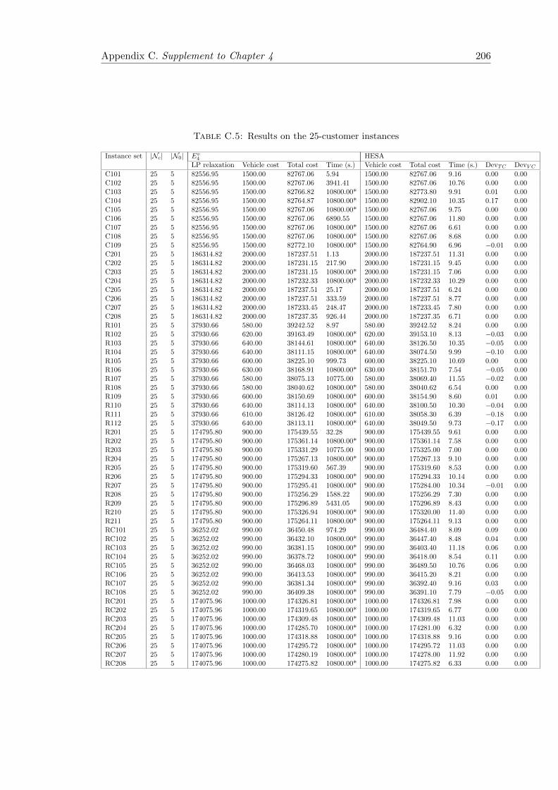
Appendix C. Supplement to Chapter 4 206
Table C.5: Results on the 25-customer instances
Instance set |Nc| |N0| Ev4 HESALP relaxation Vehicle cost Total cost Time (s.) Vehicle cost Total cost Time (s.) DevTC DevV C
C101 25 5 82556.95 1500.00 82767.06 5.94 1500.00 82767.06 9.16 0.00 0.00C102 25 5 82556.95 1500.00 82767.06 3941.41 1500.00 82767.06 10.76 0.00 0.00C103 25 5 82556.95 1500.00 82766.82 10800.00* 1500.00 82773.80 9.91 0.01 0.00C104 25 5 82556.95 1500.00 82764.87 10800.00* 1500.00 82902.10 10.35 0.17 0.00C105 25 5 82556.95 1500.00 82767.06 10800.00* 1500.00 82767.06 9.75 0.00 0.00C106 25 5 82556.95 1500.00 82767.06 6890.55 1500.00 82767.06 11.80 0.00 0.00C107 25 5 82556.95 1500.00 82767.06 10800.00* 1500.00 82767.06 6.61 0.00 0.00C108 25 5 82556.95 1500.00 82767.06 10800.00* 1500.00 82767.06 8.68 0.00 0.00C109 25 5 82556.95 1500.00 82772.10 10800.00* 1500.00 82764.90 6.96 −0.01 0.00C201 25 5 186314.82 2000.00 187237.51 1.13 2000.00 187237.51 11.31 0.00 0.00C202 25 5 186314.82 2000.00 187231.15 217.90 2000.00 187231.15 9.45 0.00 0.00C203 25 5 186314.82 2000.00 187231.15 10800.00* 2000.00 187231.15 7.06 0.00 0.00C204 25 5 186314.82 2000.00 187232.33 10800.00* 2000.00 187232.33 10.29 0.00 0.00C205 25 5 186314.82 2000.00 187237.51 25.17 2000.00 187237.51 6.24 0.00 0.00C206 25 5 186314.82 2000.00 187237.51 333.59 2000.00 187237.51 8.77 0.00 0.00C207 25 5 186314.82 2000.00 187233.45 248.47 2000.00 187233.45 7.80 0.00 0.00C208 25 5 186314.82 2000.00 187237.35 926.44 2000.00 187237.35 6.71 0.00 0.00R101 25 5 37930.66 580.00 39242.52 8.97 580.00 39242.52 8.24 0.00 0.00R102 25 5 37930.66 620.00 39163.49 10800.00* 620.00 39153.10 8.13 −0.03 0.00R103 25 5 37930.66 640.00 38144.61 10800.00* 640.00 38126.50 10.35 −0.05 0.00R104 25 5 37930.66 640.00 38111.15 10800.00* 640.00 38074.50 9.99 −0.10 0.00R105 25 5 37930.66 600.00 38225.10 999.73 600.00 38225.10 10.69 0.00 0.00R106 25 5 37930.66 630.00 38168.91 10800.00* 630.00 38151.70 7.54 −0.05 0.00R107 25 5 37930.66 580.00 38075.13 10775.00 580.00 38069.40 11.55 −0.02 0.00R108 25 5 37930.66 580.00 38040.62 10800.00* 580.00 38040.62 6.54 0.00 0.00R109 25 5 37930.66 600.00 38150.69 10800.00* 600.00 38154.90 8.60 0.01 0.00R110 25 5 37930.66 640.00 38114.13 10800.00* 640.00 38100.50 10.30 −0.04 0.00R111 25 5 37930.66 610.00 38126.42 10800.00* 610.00 38058.30 6.39 −0.18 0.00R112 25 5 37930.66 640.00 38113.11 10800.00* 640.00 38049.50 9.73 −0.17 0.00R201 25 5 174795.80 900.00 175439.55 32.28 900.00 175439.55 9.61 0.00 0.00R202 25 5 174795.80 900.00 175361.14 10800.00* 900.00 175361.14 7.58 0.00 0.00R203 25 5 174795.80 900.00 175331.29 10775.00 900.00 175325.00 7.00 0.00 0.00R204 25 5 174795.80 900.00 175267.13 10800.00* 900.00 175267.13 9.10 0.00 0.00R205 25 5 174795.80 900.00 175319.60 567.39 900.00 175319.60 8.53 0.00 0.00R206 25 5 174795.80 900.00 175294.33 10800.00* 900.00 175294.33 10.14 0.00 0.00R207 25 5 174795.80 900.00 175295.41 10800.00* 900.00 175284.00 10.34 −0.01 0.00R208 25 5 174795.80 900.00 175256.29 1588.22 900.00 175256.29 7.30 0.00 0.00R209 25 5 174795.80 900.00 175296.89 5431.05 900.00 175296.89 8.43 0.00 0.00R210 25 5 174795.80 900.00 175326.94 10800.00* 900.00 175320.00 11.40 0.00 0.00R211 25 5 174795.80 900.00 175264.11 10800.00* 900.00 175264.11 9.13 0.00 0.00RC101 25 5 36252.02 990.00 36450.48 974.29 990.00 36484.40 8.09 0.09 0.00RC102 25 5 36252.02 990.00 36432.10 10800.00* 990.00 36447.40 8.48 0.04 0.00RC103 25 5 36252.02 990.00 36381.15 10800.00* 990.00 36403.40 11.18 0.06 0.00RC104 25 5 36252.02 990.00 36378.72 10800.00* 990.00 36418.00 8.54 0.11 0.00RC105 25 5 36252.02 990.00 36468.03 10800.00* 990.00 36489.50 10.76 0.06 0.00RC106 25 5 36252.02 990.00 36413.53 10800.00* 990.00 36415.20 8.21 0.00 0.00RC107 25 5 36252.02 990.00 36381.34 10800.00* 990.00 36392.40 9.16 0.03 0.00RC108 25 5 36252.02 990.00 36409.38 10800.00* 990.00 36391.10 7.79 −0.05 0.00RC201 25 5 174075.96 1000.00 174326.81 10800.00* 1000.00 174326.81 7.98 0.00 0.00RC202 25 5 174075.96 1000.00 174319.65 10800.00* 1000.00 174319.65 6.77 0.00 0.00RC203 25 5 174075.96 1000.00 174309.48 10800.00* 1000.00 174309.48 11.03 0.00 0.00RC204 25 5 174075.96 1000.00 174285.70 10800.00* 1000.00 174281.00 6.32 0.00 0.00RC205 25 5 174075.96 1000.00 174318.88 10800.00* 1000.00 174318.88 9.16 0.00 0.00RC206 25 5 174075.96 1000.00 174295.72 10800.00* 1000.00 174295.72 11.03 0.00 0.00RC207 25 5 174075.96 1000.00 174280.19 10800.00* 1000.00 174278.00 11.92 0.00 0.00RC208 25 5 174075.96 1000.00 174275.82 10800.00* 1000.00 174275.82 6.33 0.00 0.00
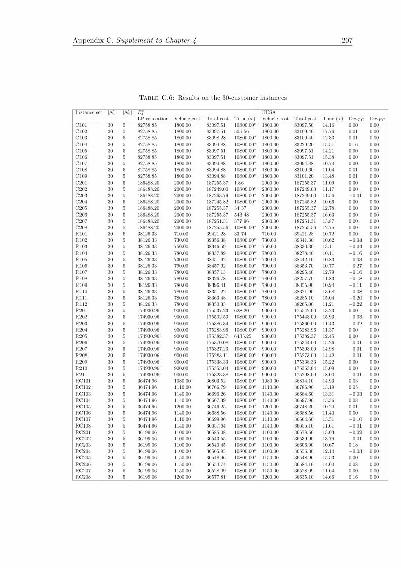
Appendix C. Supplement to Chapter 4 207
Table C.6: Results on the 30-customer instances
Instance set |Nc| |N0| Ev4 HESALP relaxation Vehicle cost Total cost Time (s.) Vehicle cost Total cost Time (s.) DevTC DevV C
C101 30 5 82758.85 1800.00 83097.51 10800.00* 1800.00 83097.50 14.16 0.00 0.00C102 30 5 82758.85 1800.00 83097.51 505.56 1800.00 83109.40 17.76 0.01 0.00C103 30 5 82758.85 1800.00 83098.28 10800.00* 1800.00 83109.40 12.33 0.01 0.00C104 30 5 82758.85 1800.00 83094.88 10800.00* 1800.00 83229.20 15.51 0.16 0.00C105 30 5 82758.85 1800.00 83097.51 10800.00* 1800.00 83097.51 14.21 0.00 0.00C106 30 5 82758.85 1800.00 83097.51 10800.00* 1800.00 83097.51 15.38 0.00 0.00C107 30 5 82758.85 1800.00 83094.88 10800.00* 1800.00 83094.88 10.70 0.00 0.00C108 30 5 82758.85 1800.00 83094.88 10800.00* 1800.00 83100.60 11.04 0.01 0.00C109 30 5 82758.85 1800.00 83094.88 10800.00* 1800.00 83101.20 13.48 0.01 0.00C201 30 5 186488.20 2000.00 187255.37 1.86 2000.00 187255.37 11.09 0.00 0.00C202 30 5 186488.20 2000.00 187249.00 10800.00* 2000.00 187249.00 11.17 0.00 0.00C203 30 5 186488.20 2000.00 187263.79 10800.00* 2000.00 187249.00 11.56 −0.01 0.00C204 30 5 186488.20 2000.00 187245.82 10800.00* 2000.00 187245.82 10.66 0.00 0.00C205 30 5 186488.20 2000.00 187255.37 34.37 2000.00 187255.37 12.78 0.00 0.00C206 30 5 186488.20 2000.00 187255.37 543.48 2000.00 187255.37 16.63 0.00 0.00C207 30 5 186488.20 2000.00 187251.31 377.96 2000.00 187251.31 13.87 0.00 0.00C208 30 5 186488.20 2000.00 187255.56 10800.00* 2000.00 187255.56 12.75 0.00 0.00R101 30 5 38126.33 710.00 39421.28 33.74 710.00 39421.28 10.72 0.00 0.00R102 30 5 38126.33 730.00 39356.38 10800.00* 730.00 39341.30 10.62 −0.04 0.00R103 30 5 38126.33 750.00 38346.59 10800.00* 750.00 38330.30 13.11 −0.04 0.00R104 30 5 38126.33 780.00 38337.89 10800.00* 780.00 38278.40 10.11 −0.16 0.00R105 30 5 38126.33 730.00 38451.92 10800.00* 730.00 38442.10 10.83 −0.03 0.00R106 30 5 38126.33 790.00 38457.92 10800.00* 790.00 38353.70 10.77 −0.27 0.00R107 30 5 38126.33 780.00 38357.13 10800.00* 780.00 38295.40 12.79 −0.16 0.00R108 30 5 38126.33 780.00 38326.78 10800.00* 780.00 38257.70 11.83 −0.18 0.00R109 30 5 38126.33 780.00 38396.41 10800.00* 780.00 38355.90 10.24 −0.11 0.00R110 30 5 38126.33 780.00 38351.22 10800.00* 780.00 38321.90 13.68 −0.08 0.00R111 30 5 38126.33 780.00 38363.48 10800.00* 780.00 38285.10 15.04 −0.20 0.00R112 30 5 38126.33 780.00 38350.33 10800.00* 780.00 38265.00 11.21 −0.22 0.00R201 30 5 174930.96 900.00 175537.23 628.20 900.00 175542.00 13.23 0.00 0.00R202 30 5 174930.96 900.00 175502.53 10800.00* 900.00 175443.00 15.93 −0.03 0.00R203 30 5 174930.96 900.00 175386.34 10800.00* 900.00 175360.00 11.43 −0.02 0.00R204 30 5 174930.96 900.00 175283.96 10800.00* 900.00 175283.96 11.37 0.00 0.00R205 30 5 174930.96 900.00 175382.37 6435.25 900.00 175382.37 12.45 0.00 0.00R206 30 5 174930.96 900.00 175370.08 10800.00* 900.00 175344.00 15.26 −0.01 0.00R207 30 5 174930.96 900.00 175327.23 10800.00* 900.00 175303.00 14.98 −0.01 0.00R208 30 5 174930.96 900.00 175283.11 10800.00* 900.00 175273.00 14.42 −0.01 0.00R209 30 5 174930.96 900.00 175338.33 10800.00* 900.00 175338.33 15.22 0.00 0.00R210 30 5 174930.96 900.00 175353.04 10800.00* 900.00 175353.04 15.09 0.00 0.00R211 30 5 174930.96 900.00 175323.38 10800.00* 900.00 175298.00 18.00 −0.01 0.00RC101 30 5 36474.96 1080.00 36803.52 10800.00* 1080.00 36814.10 14.93 0.03 0.00RC102 30 5 36474.96 1110.00 36766.79 10800.00* 1110.00 36786.90 13.19 0.05 0.00RC103 30 5 36474.96 1140.00 36696.26 10800.00* 1140.00 36684.60 13.31 −0.03 0.00RC104 30 5 36474.96 1140.00 36667.39 10800.00* 1140.00 36697.90 13.36 0.08 0.00RC105 30 5 36474.96 1200.00 36746.25 10800.00* 1200.00 36748.20 10.20 0.01 0.00RC106 30 5 36474.96 1140.00 36688.56 10800.00* 1140.00 36688.56 11.40 0.00 0.00RC107 30 5 36474.96 1110.00 36699.96 10800.00* 1110.00 36664.60 13.51 −0.10 0.00RC108 30 5 36474.96 1140.00 36657.64 10800.00* 1140.00 36655.10 11.61 −0.01 0.00RC201 30 5 36199.06 1100.00 36585.08 10800.00* 1100.00 36578.50 13.03 −0.02 0.00RC202 30 5 36199.06 1100.00 36543.55 10800.00* 1100.00 36539.90 13.79 −0.01 0.00RC203 30 5 36199.06 1100.00 36540.45 10800.00* 1100.00 36606.90 10.67 0.18 0.00RC204 30 5 36199.06 1100.00 36565.95 10800.00* 1100.00 36556.30 12.14 −0.03 0.00RC205 30 5 36199.06 1150.00 36548.96 10800.00* 1150.00 36548.96 15.53 0.00 0.00RC206 30 5 36199.06 1150.00 36554.74 10800.00* 1150.00 36584.10 14.00 0.08 0.00RC207 30 5 36199.06 1150.00 36528.09 10800.00* 1150.00 36528.09 11.64 0.00 0.00RC208 30 5 36199.06 1200.00 36577.81 10800.00* 1200.00 36635.10 14.66 0.16 0.00

Appendix C. Supplement to Chapter 4 208
Table C.7: Results on the 50-customer instances
Instance set |Nc| |N0| Ev4 HESALP relaxation Vehicle cost Total cost Time (s.) Vehicle cost Total cost Time (s.) DevTC DevV C
C101 50 7 41386.56 2700.00 41865.26 398.97 2700.00 41892.30 70.96 0.06 0.00C102 50 7 41386.56 2700.00 41859.80 10800.00* 2700.00 41859.80 103.47 0.00 0.00C103 50 7 41386.56 2900.00 41968.98 10800.00* 2900.00 41922.80 61.00 −0.11 0.00C104 50 7 41386.56 2700.00 41890.98 10800.00* 2700.00 42000.50 114.55 0.26 0.00C105 50 7 41386.56 2700.00 41852.69 10800.00* 2700.00 41852.69 81.52 0.00 0.00C106 50 7 41386.56 2700.00 41853.79 10800.00* 2700.00 41853.79 95.53 0.00 0.00C107 50 7 41386.56 2700.00 41851.28 10800.00* 2700.00 41903.50 106.71 0.12 0.00C108 50 7 41386.56 2700.00 41850.25 10800.00* 2700.00 41895.50 105.26 0.11 0.00C109 50 7 41386.56 2700.00 41890.31 10800.00* 2700.00 42016.20 98.83 0.30 0.00C201 50 7 92446.10 2400.00 92880.93 6.21 2400.00 92880.93 109.43 0.00 0.00C202 50 7 92446.10 3000.00 93384.81 10800.00* 2400.00 92825.00 62.39 −0.60 −20.00C203 50 7 92446.10 3400.00 93869.63 10800.00* 2400.00 92818.60 118.84 −1.12 −29.41C204 50 7 92446.10 3000.00 93470.84 10800.00* 2400.00 92770.40 115.62 −0.75 −20.00C205 50 7 92446.10 3000.00 93391.05 10800.00* 2400.00 92876.60 115.28 −0.55 −20.00C206 50 7 92446.10 3000.00 93391.05 10800.00* 2400.00 92811.40 66.99 −0.62 −20.00C207 50 7 92446.10 3000.00 93378.45 10800.00* 2400.00 92798.30 117.47 −0.62 −20.00C208 50 7 92446.10 3000.00 93390.88 10800.00* 2400.00 92798.40 87.68 −0.63 −20.00R101 50 7 38870.22 1280.00 40443.15 10800.00* 1250.00 40443.15 83.30 0.00 −2.34R102 50 7 38870.22 1380.00 40440.99 10800.00* 1350.00 40328.30 95.11 −0.28 −2.17R103 50 7 38870.22 1430.00 41424.71 10800.00* 1280.00 40195.20 83.30 −2.97 −10.49R104 50 7 38870.22 1360.00 39368.54 10800.00* 1370.00 39155.50 112.85 −0.54 0.74R105 50 7 38870.22 1280.00 39380.48 10800.00* 1260.00 39356.20 113.54 −0.06 −1.56R106 50 7 38870.22 1320.00 39459.31 10800.00* 1280.00 39263.10 119.24 −0.50 −3.03R107 50 7 38870.22 1430.00 39443.09 10800.00* 1310.00 39152.30 92.82 −0.74 −8.39R108 50 7 38870.22 1300.00 39322.58 10800.00* 1370.00 39157.10 104.15 −0.42 5.38R109 50 7 38870.22 1350.00 39322.03 10800.00* 1280.00 39250.70 72.21 −0.18 −5.19R110 50 7 38870.22 1320.00 39411.26 10800.00* 1310.00 39211.80 61.42 −0.51 −0.76R111 50 7 38870.22 1300.00 39255.20 10800.00* 1280.00 39179.70 84.72 −0.19 −1.54R112 50 7 38870.22 1450.00 39403.04 10800.00* 1280.00 39170.50 97.18 −0.59 −11.72R201 50 7 175518.42 1350.00 176218.56 10800.00* 1350.00 176218.56 86.87 0.00 0.00R202 50 7 175518.42 2050.00 177013.02 10800.00* 1350.00 176088.00 91.59 −0.52 −34.15R203 50 7 175518.42 1350.00 176249.23 10800.00* 1350.00 175995.00 93.72 −0.14 0.00R204 50 7 175518.42 1350.00 175917.21 10800.00* 1350.00 175866.00 118.70 −0.03 0.00R205 50 7 175518.42 1350.00 176200.21 10800.00* 1350.00 176061.00 90.21 −0.08 0.00R206 50 7 175518.42 1350.00 176081.07 10800.00* 1350.00 176000.00 117.02 −0.05 0.00R207 50 7 175518.42 2050.00 176815.10 10800.00* 1350.00 175932.00 119.13 −0.50 −34.15R208 50 7 175518.42 1350.00 175962.50 10800.00* 1350.00 175855.00 63.31 −0.06 0.00R209 50 7 175518.42 1350.00 176089.81 10800.00* 1350.00 175995.00 69.61 −0.05 0.00R210 50 7 175518.42 1600.00 176374.18 10800.00* 1350.00 175994.00 82.15 −0.22 −15.63R211 50 7 175518.42 1800.00 176704.38 10800.00* 1350.00 175905.00 87.41 −0.45 −25.00RC101 50 7 19574.34 1950.00 21031.12 10800.00* 1860.00 20978.50 83.08 −0.25 −4.62RC102 50 7 19574.34 2280.00 21334.83 10800.00* 1950.00 20892.30 63.81 −2.07 −14.47RC103 50 7 19574.34 2130.00 38142.81 10800.00* 1950.00 20778.80 74.35 −45.52 −8.45RC104 50 7 19574.34 2250.00 20274.62 10800.00* 2010.00 20020.00 105.47 −1.26 −10.67RC105 50 7 19574.34 2010.00 20991.89 10800.00* 1950.00 20889.10 72.03 −0.49 −2.99RC106 50 7 19574.34 2040.00 20325.56 10800.00* 1950.00 20223.20 76.47 −0.50 −4.41RC107 50 7 19574.34 2040.00 20291.25 10800.00* 1860.00 20085.60 61.74 −1.01 −8.82RC108 50 7 19574.34 1950.00 20064.39 10800.00* 1980.00 20018.40 75.42 −0.23 1.54RC201 50 7 87065.42 1700.00 87586.41 10800.00* 1800.00 87641.90 94.32 0.06 5.88RC202 50 7 87065.42 1900.00 87992.95 10800.00* 1800.00 87546.10 65.43 −0.51 −5.26RC203 50 7 87065.42 2250.00 88339.08 10800.00* 1900.00 87558.60 114.14 −0.88 −15.56RC204 50 7 87065.42 3550.00 89274.98 10800.00* 1900.00 87456.90 61.20 −2.04 −46.48RC205 50 7 87065.42 1900.00 87784.60 10800.00* 1800.00 87530.90 76.40 −0.29 −5.26RC206 50 7 87065.42 1750.00 87989.08 10800.00* 1900.00 87619.80 69.17 −0.42 8.57RC207 50 7 87065.42 1850.00 88092.32 10800.00* 1900.00 87469.30 104.49 −0.71 2.70RC208 50 7 87065.42 2550.00 88410.89 10800.00* 1950.00 87464.80 99.78 −1.07 −23.53

Appendix C. Supplement to Chapter 4 209
Table C.8: Results on the 75-customer instances
Instance set |Nc| |N0| Ev4 HESALP relaxation Vehicle cost Total cost Time (s.) Vehicle cost Total cost Time (s.) DevTC DevV C
C101 75 8 82857.15 4200.00 83309.83 10800.00* 4200.00 83376.60 187.36 0.08 0.00C102 75 8 82857.15 4200.00 83343.28 10800.00* 4200.00 83389.00 185.65 0.05 0.00C103 75 8 82857.15 5350.00 84468.47 10800.00* 4200.00 83321.10 157.32 −1.36 −21.50C104 75 8 82857.15 5450.00 84670.05 10800.00* 4800.00 83766.60 159.44 −1.07 −11.93C105 75 8 82857.15 4200.00 83311.92 10800.00* 4200.00 83489.80 164.07 0.21 0.00C106 75 8 82857.15 4200.00 83307.33 10800.00* 4200.00 83372.90 184.56 0.08 0.00C107 75 8 82857.15 4200.00 83308.44 10800.00* 4200.00 83632.90 179.85 0.39 0.00C108 75 8 82857.15 4200.00 83450.51 10800.00* 4200.00 83411.10 176.41 −0.05 0.00C109 75 8 82857.15 4600.00 83792.90 10800.00* 4400.00 83555.50 165.48 −0.28 −4.35C201 75 8 188792.53 4000.00 189585.40 10800.00* 3800.00 189401.00 163.23 −0.10 −5.00C202 75 8 188792.53 6400.00 192152.42 10800.00* 3800.00 189371.00 161.08 −1.45 −40.63C203 75 8 188792.53 7500.00 193453.62 10800.00* 3800.00 189360.00 174.90 −2.12 −49.33C204 75 8 188792.53 13800.00 200531.39 10800.00* 3800.00 189328.00 141.79 −5.59 −72.46C205 75 8 188792.53 4000.00 189582.69 10800.00* 3800.00 189400.00 144.57 −0.10 −5.00C206 75 8 188792.53 5000.00 190731.82 10800.00* 3800.00 189376.00 180.62 −0.71 −24.00C207 75 8 188792.53 7100.00 193275.65 10800.00* 3800.00 189390.00 170.03 −2.01 −46.48C208 75 8 188792.53 8800.00 194531.18 10800.00* 3800.00 189372.00 186.91 −2.65 −56.82R101 75 8 38056.29 1970.00 40600.20 10800.00* 1880.00 40609.90 189.28 0.02 −4.57R102 75 8 38056.29 2040.00 40913.94 10800.00* 1900.00 40437.50 162.13 −1.16 −6.86R103 75 8 38056.29 8370.00 176468.82 10800.00* 1960.00 40252.60 147.57 −77.19 −76.58R104 75 8 38056.29 3290.00 40584.42 10800.00* 2010.00 40256.90 188.58 −0.81 −38.91R105 75 8 38056.29 2060.00 40643.62 10800.00* 1920.00 40368.50 172.37 −0.68 −6.80R106 75 8 38056.29 4140.00 103148.58 10800.00* 1920.00 40295.60 157.16 −60.93 −53.62R107 75 8 38056.29 4860.00 81617.99 10800.00* 2010.00 40332.90 173.12 −50.58 −58.64R108 75 8 38056.29 5390.00 61602.75 10800.00* 2120.00 40234.80 156.94 −34.69 −60.67R109 75 8 38056.29 2760.00 39933.80 10800.00* 1980.00 38825.00 171.10 −2.78 −28.26R110 75 8 38056.29 4660.00 42288.53 10800.00* 1960.00 38715.10 182.79 −8.45 −57.94R111 75 8 38056.29 5290.00 61206.47 10800.00* 2010.00 40281.90 186.65 −34.19 −62.00R112 75 8 38056.29 3670.00 40971.58 10800.00* 1960.00 38660.40 177.68 −5.64 −46.59R201 75 8 174160.82 2250.00 175775.01 10800.00* 1800.00 174859.00 152.31 −0.52 −20.00R202 75 8 174160.82 5900.00 179505.22 10800.00* 1800.00 174767.00 145.66 −2.64 −69.49R203 75 8 174160.82 8700.00 182253.80 10800.00* 1800.00 174601.00 171.49 −4.20 −79.31R204 75 8 174160.82 5000.00 177907.86 10800.00* 1800.00 174472.00 173.79 −1.93 −64.00R205 75 8 174160.82 2950.00 176368.20 10800.00* 1800.00 174659.00 141.53 −0.97 −38.98R206 75 8 174160.82 3700.00 176973.52 10800.00* 1800.00 174597.00 178.87 −1.34 −51.35R207 75 8 174160.82 4650.00 178021.12 10800.00* 1800.00 174524.00 173.78 −1.96 −61.29R208 75 8 174160.82 5750.00 178926.32 10800.00* 1800.00 174445.00 150.08 −2.50 −68.70R209 75 8 174160.82 6550.00 179798.66 10800.00* 1800.00 174563.00 176.27 −2.91 −72.52R210 75 8 174160.82 5700.00 179194.44 10800.00* 1800.00 174605.00 150.63 −2.56 −68.42R211 75 8 174160.82 6550.00 179843.07 10800.00* 1800.00 174522.00 166.47 −2.96 −72.52RC101 75 8 38233.86 2520.00 39061.10 10800.00* 2520.00 38940.60 172.15 −0.31 0.00RC102 75 8 38233.86 2640.00 39221.20 10800.00* 2550.00 38832.50 174.34 −0.99 −3.41RC103 75 8 38233.86 3510.00 39820.43 10800.00* 2580.00 38717.80 183.92 −2.77 −26.50RC104 75 8 38233.86 3480.00 39830.82 10800.00* 2700.00 38677.30 158.68 −2.90 −22.41RC105 75 8 38233.86 2760.00 39258.60 10800.00* 2580.00 38866.70 167.90 −1.00 −6.52RC106 75 8 38233.86 2910.00 39318.93 10800.00* 2610.00 38795.00 183.80 −1.33 −10.31RC107 75 8 38233.86 3390.00 39692.26 10800.00* 2670.00 38676.20 165.33 −2.56 −21.24RC108 75 8 38233.86 3480.00 39984.80 10800.00* 2550.00 38645.00 186.19 −3.35 −26.72RC201 75 8 173677.24 2250.00 174872.25 10800.00* 2350.00 174546.00 159.46 −0.19 4.44RC202 75 8 173677.24 4700.00 177692.77 10800.00* 2350.00 174332.00 162.91 −1.89 −50.00RC203 75 8 173677.24 5550.00 178208.59 10800.00* 2400.00 174373.00 173.16 −2.15 −56.76RC204 75 8 173677.24 6250.00 179071.17 10800.00* 2550.00 174241.00 185.53 −2.70 −59.20RC205 75 8 173677.24 2900.00 175681.10 10800.00* 2400.00 174444.00 152.35 −0.70 −17.24RC206 75 8 173677.24 2650.00 175218.43 10800.00* 2450.00 174419.00 147.26 −0.46 −7.55RC207 75 8 173677.24 5300.00 178097.38 10800.00* 2550.00 174346.00 144.99 −2.11 −51.89RC208 75 8 173677.24 3800.00 176137.37 10800.00* 2550.00 174242.00 155.45 −1.08 −32.89

Appendix C. Supplement to Chapter 4 210
Table C.9: Results on the 100-customer instances
Instance set |Nc| |N0| Ev4 HESALP relaxation Vehicle cost Total cost Time (s.) Vehicle cost Total cost Time (s.) DevTC DevV C
C101 100 10 84345.45 5700.00 85199.09 10800.00* 5700.00 85199.09 297.32 0.00 0.00C102 100 10 84345.45 6300.00 86605.08 10800.00* 5700.00 85209.00 304.48 −1.61 −9.52C103 100 10 84345.45 8300.00 88128.63 10800.00* 5700.00 85190.80 305.06 −3.33 −31.33C104 100 10 84345.45 11000.00 90622.34 10800.00* 6500.00 85509.90 319.80 −5.64 −40.91C105 100 10 84345.45 5700.00 85258.60 10800.00* 5700.00 85208.50 319.99 −0.06 0.00C106 100 10 84345.45 5700.00 85461.36 10800.00* 5700.00 85204.90 309.38 −0.30 0.00C107 100 10 84345.45 5700.00 85306.67 10800.00* 5700.00 85167.30 307.85 −0.16 0.00C108 100 10 84345.45 5900.00 85570.18 10800.00* 5700.00 85222.80 294.20 −0.41 −3.39C109 100 10 84345.45 9100.00 89617.66 10800.00* 5700.00 85198.00 312.34 −4.93 −37.36C201 100 10 190083.07 6000.00 191687.14 10800.00* 5200.00 190876.00 271.94 −0.42 −13.33C202 100 10 190074.71 9900.00 195858.81 10800.00* 5200.00 190865.00 259.04 −2.55 −47.47C203 100 10 190075.95 17900.00 304096.37 10800.00* 5200.00 190864.00 308.09 −37.24 −70.95C204 100 10 190074.71 98300.00 1154483.31 10800.00* 5200.00 190848.00 337.23 −83.47 −94.71C205 100 10 190077.15 8400.00 194711.89 10800.00* 5200.00 190863.00 304.44 −1.98 −38.10C206 100 10 190084.61 15600.00 202111.00 10800.00* 5200.00 190861.00 321.63 −5.57 −66.67C207 100 10 190075.31 13200.00 199617.46 10800.00* 5200.00 190856.00 330.40 −4.39 −60.61C208 100 10 190074.82 13800.00 200924.51 10800.00* 5200.00 190866.00 333.46 −5.01 −62.32R101 100 10 39159.76 2770.00 42095.43 10800.00* 2560.00 41782.20 292.25 −0.74 −7.58R102 100 10 39146.09 7090.00 105133.04 10800.00* 2600.00 41577.10 324.69 −60.45 −63.33R103 100 10 39149.89 10860.00 225357.73 10800.00* 2620.00 41398.40 293.22 −81.63 −75.87R104 100 10 39151.07 12740.00 227609.71 10800.00* 2680.00 41269.90 289.51 −81.87 −78.96R105 100 10 39154.42 4790.00 81860.12 10800.00* 2670.00 41522.20 250.56 −49.28 −44.26R106 100 10 39145.82 12070.00 226936.85 10800.00* 2650.00 41397.50 291.75 −81.76 −78.04R107 100 10 39145.98 14680.00 230534.40 10800.00* 2680.00 41329.90 339.02 −82.07 −81.74R108 100 10 39148.67 12390.00 227135.02 10800.00* 2680.00 40574.50 336.96 −82.14 −78.37R109 100 10 39161.60 8300.00 106140.17 10800.00* 2710.00 40135.40 247.20 −62.19 −67.35R110 100 10 39146.09 8800.00 68339.42 10800.00* 2600.00 40052.30 267.95 −41.39 −70.45R111 100 10 39145.98 12590.00 228378.35 10800.00* 2600.00 40614.10 296.14 −82.22 −79.35R112 100 10 39165.22 10900.00 226034.92 10800.00* 2730.00 40015.60 250.16 −82.30 −74.95R201 100 10 174794.14 6400.00 180128.14 10800.00* 2250.00 175457.00 329.90 −2.59 −64.84R202 100 10 174794.09 14450.00 188288.16 10800.00* 2250.00 175303.00 256.58 −6.90 −84.43R203 100 10 174794.09 12850.00 186985.40 10800.00* 2250.00 175186.00 289.80 −6.31 −82.49R204 100 10 174794.09 11250.00 184455.99 10800.00* 2250.00 175037.00 297.46 −5.11 −80.00R205 100 10 174794.09 12450.00 186185.59 10800.00* 2250.00 175237.00 339.93 −5.88 −81.93R206 100 10 174794.14 14150.00 187873.20 10800.00* 2250.00 175168.00 268.04 −6.76 −84.10R207 100 10 174794.09 11950.00 185389.11 10800.00* 2250.00 175096.00 270.70 −5.55 −81.17R208 100 10 174794.09 7500.00 180572.09 10800.00* 2250.00 175010.00 322.05 −3.08 −70.00R209 100 10 174794.09 14700.00 188632.91 10800.00* 2250.00 175156.00 288.98 −7.14 −84.69R210 100 10 174794.14 14850.00 188607.92 10800.00* 2250.00 175189.00 311.21 −7.11 −84.85R211 100 10 174794.14 12200.00 185459.83 10800.00* 2250.00 175051.00 247.03 −5.61 −81.56RC101 100 10 39180.69 3510.00 40800.29 10800.00* 3300.00 40111.60 323.52 −1.69 −5.98RC102 100 10 39186.00 7530.00 44712.85 10800.00* 3330.00 39940.70 328.25 −10.67 −55.78RC103 100 10 39199.13 7890.00 70169.17 10800.00* 3510.00 39828.90 316.82 −43.24 −55.51RC104 100 10 39181.17 7530.00 67342.83 10800.00* 3420.00 39727.00 317.03 −41.01 −54.58RC105 100 10 39203.16 4710.00 42222.87 10800.00* 3390.00 39990.10 281.31 −5.29 −28.03RC106 100 10 39176.91 5100.00 42502.09 10800.00* 3420.00 39912.40 323.17 −6.09 −32.94RC107 100 10 39176.91 6930.00 44066.07 10800.00* 3420.00 39827.50 275.89 −9.62 −50.65RC108 100 10 39187.37 5790.00 42617.67 10800.00* 3450.00 39775.20 282.44 −6.67 −40.41RC201 100 10 174428.16 4700.00 177634.48 10800.00* 3150.00 175461.00 282.26 −1.22 −32.98RC202 100 10 174429.52 8500.00 181651.48 10800.00* 3100.00 175284.00 278.25 −3.51 −63.53RC203 100 10 174428.48 11700.00 185169.73 10800.00* 3250.00 175271.00 313.55 −5.35 −72.22RC204 100 10 174435.83 37550.00 873972.63 10800.00* 1350.00 173214.00 260.57 −80.18 −96.40RC205 100 10 174432.47 9850.00 183169.93 10800.00* 3100.00 175409.00 317.51 −4.24 −68.53RC206 100 10 174427.49 11600.00 184800.00 10800.00* 3150.00 175333.00 318.89 −5.12 −72.84RC207 100 10 174426.83 6350.00 179681.12 10800.00* 3250.00 175280.00 300.42 −2.45 −48.82RC208 100 10 174436.39 10300.00 183920.02 10800.00* 3350.00 175210.00 287.60 −4.74 −67.48

Appendix D
Supplement to Chapter 5
Tables D.1 to D.4 present the detailed computational results on the 75, 100, 150, and
200-node FSMPRP instances. In all tables, columns TD, CO2, FEC, DC, VC, TC and
Time are as explained in the main body of text. Column Mix shows the resulting fleet
composition where L, M and H refer to light, medium and heavy vehicles and the
subscripts denote the number of such vehicles used in the fleet.
211

Appendix D. Supplement to Chapter 5 212
TableD.1:
Com
pu
tati
on
al
resu
lts
on
the
75-n
od
eF
SM
PR
Pin
stan
ces
Inst
ance
HE
A+
+T
DC
O2
FE
CD
CV
CM
ixT
CT
ime
UK
7501
1615
.33
373.
6522
5.48
295.
0530
0M
582
0.52
2.37
UK
7502
1295
.66
289.
3217
4.59
268.
0828
2L1M
472
4.67
3.39
UK
7503
1565
.67
349.
9421
1.17
274.
5828
2L1M
476
7.75
3.56
UK
7504
1322
.99
298.
2617
9.99
274.
1728
2L1M
473
6.16
3.74
UK
7505
1559
.89
358.
8921
6.57
274.
9830
0M
579
1.56
3.27
UK
7506
1588
.73
366.
9022
1.41
287.
8830
0M
580
9.29
3.34
UK
7507
1586
.55
367.
3822
1.70
294.
2530
0M
581
5.94
2.81
UK
7508
1721
.67
361.
2821
8.01
299.
2230
6L3M
382
3.23
3.35
UK
7509
1609
.60
354.
0121
3.62
278.
5728
2L1M
477
4.19
3.49
UK
7510
1575
.76
365.
4622
0.54
285.
2330
0M
580
5.77
3.71
UK
7511
1161
.03
255.
7215
4.31
247.
3928
2L1M
468
3.70
3.47
UK
7512
1445
.46
334.
1020
1.61
260.
3830
0M
576
1.99
3.19
UK
7513
1786
.96
383.
6323
1.50
297.
8932
4L2M
485
3.39
2.59
UK
7514
1585
.74
367.
0022
1.47
279.
0630
0M
580
0.52
3.38
UK
7515
1707
.01
366.
1322
0.94
296.
4132
4L2M
484
1.35
3.32
UK
7516
1536
.76
356.
4421
5.09
277.
4530
0M
579
2.54
3.93
UK
7517
1552
.07
359.
0221
6.65
287.
9430
0M
580
4.59
2.41
UK
7518
1483
.53
327.
6019
7.69
274.
3028
2L1M
475
3.99
3.33
UK
7519
1467
.55
328.
3519
8.14
269.
8428
2L1M
474
9.99
3.49
UK
7520
1519
.60
351.
6421
2.20
280.
3830
0M
579
2.57
3.19

Appendix D. Supplement to Chapter 5 213
TableD.2:
Com
pu
tati
on
al
resu
lts
on
the
100-n
od
eF
SM
PR
Pin
stan
ces
Inst
ance
HE
A+
+T
DC
O2
FE
CD
CV
CM
ixT
CT
ime
UK
100
0120
31.4
644
4.12
268.
0037
5.10
384
L2M
510
27.1
05.
47U
K10
002
1970
.65
428.
6825
8.69
360.
1938
4L2M
510
02.8
74.
38U
K10
003
1756
.29
392.
3823
6.78
341.
3434
2L1M
592
0.11
4.65
UK
100
0416
74.2
938
4.01
231.
7335
8.58
402
L1M
699
2.32
4.74
UK
100
0515
83.7
636
8.75
222.
5234
9.04
360
M6
931.
564.
21U
K10
006
1898
.02
430.
7625
9.94
376.
3140
2L1M
610
38.2
55.
63U
K10
007
1790
.55
400.
8924
1.91
329.
4834
2L1M
591
3.39
5.19
UK
100
0819
19.8
442
4.64
256.
2534
6.27
342
L1M
594
4.51
4.52
UK
100
0916
33.2
336
4.06
219.
6932
9.33
342
L1M
589
1.02
4.69
UK
100
1019
55.7
742
9.26
259.
0434
6.34
384
L2M
598
9.38
4.19
UK
100
1119
04.8
842
9.65
259.
2737
3.71
402
L1M
610
34.9
85.
13U
K10
012
1603
.76
361.
6021
8.21
319.
7534
2L1M
587
9.96
4.62
UK
100
1319
44.8
342
4.91
256.
4136
0.45
384
L2M
510
00.8
64.
78U
K10
014
2025
.79
454.
5527
4.30
376.
1740
2L1M
610
52.4
75.
02U
K10
015
1983
.24
459.
4227
7.24
386.
7142
0M
710
83.9
55.
27U
K10
016
1695
.44
392.
0023
6.55
327.
8736
0M
692
4.42
4.73
UK
100
1719
80.2
044
7.53
270.
0638
5.27
402
L1M
610
57.3
34.
36U
K10
018
1788
.57
401.
3924
2.22
338.
5934
2L1M
592
2.81
5.01
UK
100
1916
45.8
938
2.38
230.
7533
3.86
360
M6
924.
604.
99U
K10
020
2043
.21
462.
3627
9.01
376.
7740
2L1M
610
57.7
84.
18
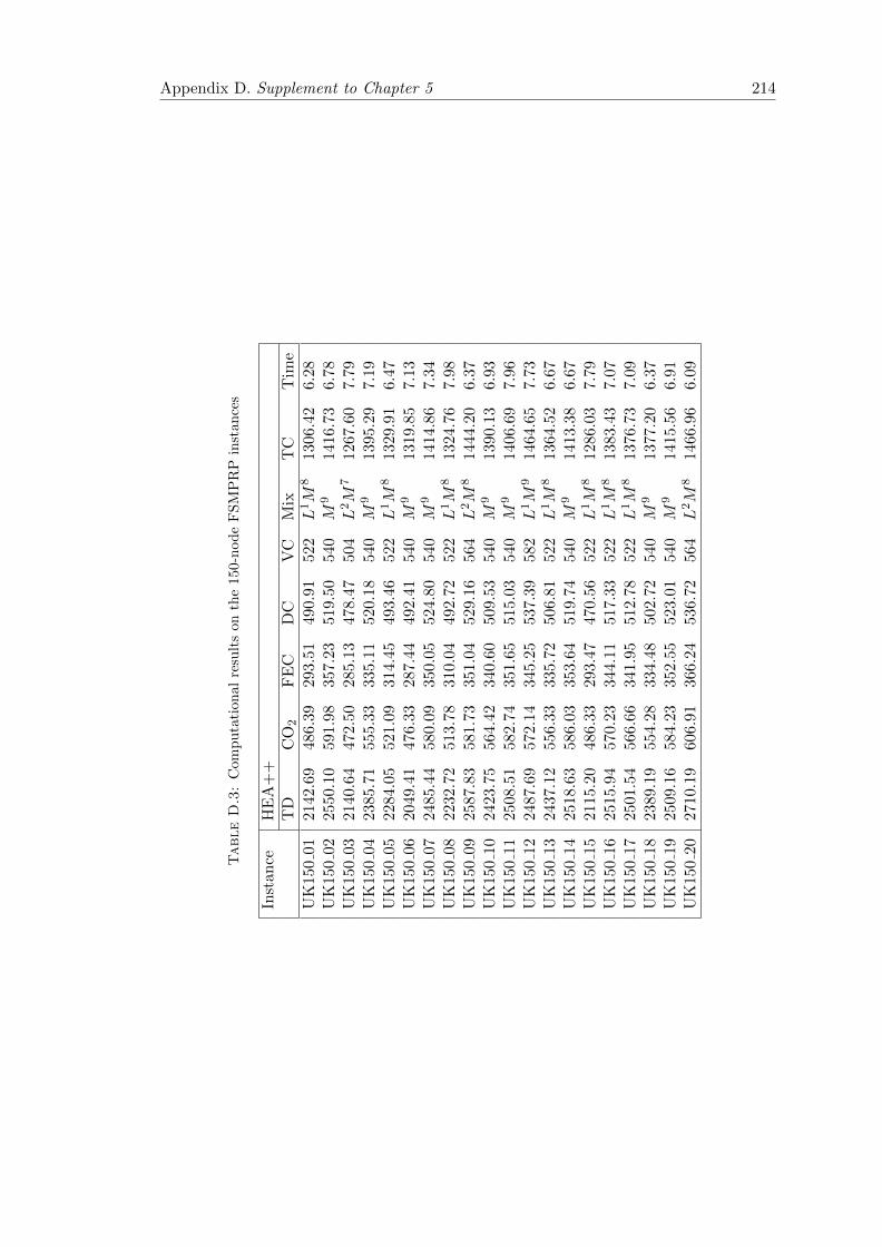
Appendix D. Supplement to Chapter 5 214
TableD.3:
Com
pu
tati
on
al
resu
lts
on
the
150-n
od
eF
SM
PR
Pin
stan
ces
Inst
ance
HE
A+
+T
DC
O2
FE
CD
CV
CM
ixT
CT
ime
UK
150
0121
42.6
948
6.39
293.
5149
0.91
522
L1M
813
06.4
26.
28U
K15
002
2550
.10
591.
9835
7.23
519.
5054
0M
914
16.7
36.
78U
K15
003
2140
.64
472.
5028
5.13
478.
4750
4L2M
712
67.6
07.
79U
K15
004
2385
.71
555.
3333
5.11
520.
1854
0M
913
95.2
97.
19U
K15
005
2284
.05
521.
0931
4.45
493.
4652
2L1M
813
29.9
16.
47U
K15
006
2049
.41
476.
3328
7.44
492.
4154
0M
913
19.8
57.
13U
K15
007
2485
.44
580.
0935
0.05
524.
8054
0M
914
14.8
67.
34U
K15
008
2232
.72
513.
7831
0.04
492.
7252
2L1M
813
24.7
67.
98U
K15
009
2587
.83
581.
7335
1.04
529.
1656
4L2M
814
44.2
06.
37U
K15
010
2423
.75
564.
4234
0.60
509.
5354
0M
913
90.1
36.
93U
K15
011
2508
.51
582.
7435
1.65
515.
0354
0M
914
06.6
97.
96U
K15
012
2487
.69
572.
1434
5.25
537.
3958
2L1M
914
64.6
57.
73U
K15
013
2437
.12
556.
3333
5.72
506.
8152
2L1M
813
64.5
26.
67U
K15
014
2518
.63
586.
0335
3.64
519.
7454
0M
914
13.3
86.
67U
K15
015
2115
.20
486.
3329
3.47
470.
5652
2L1M
812
86.0
37.
79U
K15
016
2515
.94
570.
2334
4.11
517.
3352
2L1M
813
83.4
37.
07U
K15
017
2501
.54
566.
6634
1.95
512.
7852
2L1M
813
76.7
37.
09U
K15
018
2389
.19
554.
2833
4.48
502.
7254
0M
913
77.2
06.
37U
K15
019
2509
.16
584.
2335
2.55
523.
0154
0M
914
15.5
66.
91U
K15
020
2710
.19
606.
9136
6.24
536.
7256
4L2M
814
66.9
66.
09
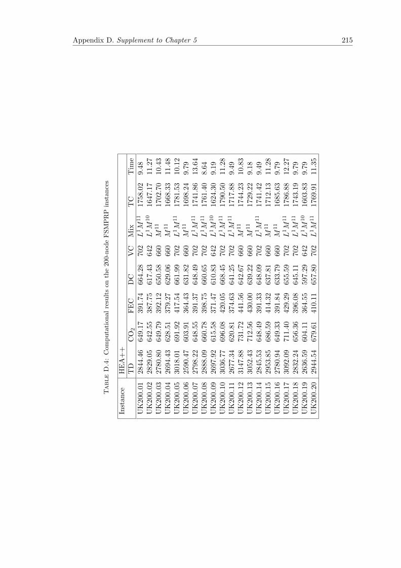
Appendix D. Supplement to Chapter 5 215
TableD.4:
Com
pu
tati
on
al
resu
lts
on
the
200-n
od
eF
SM
PR
Pin
stan
ces
Inst
an
ceH
EA
++
TD
CO
2F
EC
DC
VC
Mix
TC
Tim
e
UK
200
0128
44.4
664
9.17
391.
7466
4.28
702
L1M
11
1758
.02
9.48
UK
200
0228
29.0
564
2.55
387.
7561
7.43
642
L1M
10
1647
.17
11.2
7U
K200
0327
80.8
064
9.79
392.
1265
0.58
660
M11
1702
.70
10.4
3U
K200
0426
94.4
362
8.51
379.
2762
9.06
660
M11
1668
.33
11.4
8U
K200
0530
18.0
169
1.92
417.
5466
1.99
702
L1M
11
1781
.53
10.1
2U
K200
0625
90.4
760
3.91
364.
4363
1.82
660
M11
1698
.24
9.79
UK
200
0727
98.2
264
8.55
391.
3764
8.49
702
L1M
11
1741
.86
13.6
4U
K200
0828
88.0
966
0.78
398.
7566
0.65
702
L1M
11
1761
.40
8.64
UK
200
0926
97.9
261
5.58
371.
4761
0.83
642
L1M
10
1624
.30
9.19
UK
200
1030
36.7
769
6.08
420.
0566
8.45
702
L1M
11
1790
.50
11.2
8U
K200
1126
77.3
462
0.81
374.
6364
1.25
702
L1M
11
1717
.88
9.49
UK
200
1231
47.8
873
1.72
441.
5664
2.67
660
M11
1744
.23
10.8
3U
K200
1330
52.4
371
2.56
430.
0063
9.22
660
M11
1729
.22
9.18
UK
200
1428
45.5
364
8.49
391.
3364
8.09
702
L1M
11
1741
.42
9.49
UK
200
1529
53.8
568
6.59
414.
3263
7.81
660
M11
1712
.13
11.2
8U
K200
1627
80.9
464
9.33
391.
8463
3.79
660
M11
1685
.63
9.79
UK
200
1730
92.0
971
1.40
429.
2965
5.59
702
L1M
11
1786
.88
12.2
7U
K200
1828
32.2
465
6.36
396.
0864
5.11
702
L1M
11
1743
.19
9.79
UK
200
1926
36.5
960
4.11
364.
5559
7.29
642
L1M
10
1603
.83
9.79
UK
200
2029
44.5
467
9.61
410.
1165
7.80
702
L1M
11
1769
.91
11.3
5

Appendix E
Supplement to Chapter 6
Tables E.1–E.4 present the detailed computational results on the 25-, 50-, 75- and 100-
customer instances.
216

Appendix E. Supplement to Chapter 6 217
TableE.1:
Com
pu
tati
on
al
resu
lts
on
the
25-c
ust
om
erin
stan
ces.
Inst
an
ce|N
c||N
0|
P-L
-HA
LN
SO
pen
edT
ota
ld
ista
nce
CO
2em
issi
ons
Fu
elan
dC
O2
Dep
otco
stV
ehic
leco
stT
otal
cost
Tim
ed
epots
(km
)(k
g)em
issi
ons
cost
s(£
)(£
)(£
)(£
)(s
)
CC
251
254
(1,1
,0)
36.1
026
.12
15.7
685
00.0
010
9.00
8624
.76
5.16
CC
252
254
(2,0
,0)
45.5
910
.09
6.09
1000
0.00
109.
0010
115.
105.
20C
C25
325
4(1
,0,1
)37
.60
2.63
1.59
7000
.00
102.
0071
03.5
95.
50C
C25
425
4(1
,0,1
)40
.24
29.3
517
.71
7000
.00
109.
0071
26.7
16.
02C
C25
525
4(1
,0,1
)27
.47
39.6
223
.91
7000
.00
102.
0071
25.9
15.
42S
U25
125
4(0
,1,1
)54
.65
9.68
5.84
5500
.00
102.
0056
07.8
45.
48S
U25
225
4(1
,0,1
)63
.99
8.93
5.39
7000
.00
109.
0071
14.3
95.
48S
U25
325
4(0
,1,0
)52
.97
45.6
027
.52
3500
.00
98.0
036
25.5
25.
42S
U25
425
4(1
,1,0
)46
.88
0.15
0.09
5500
.00
102.
0056
02.0
95.
38S
U25
525
4(0
,1,1
)61
.55
38.7
823
.40
5500
.00
102.
0056
25.4
05.
44R
25
125
4(0
,1,0
)73
.07
28.6
317
.28
3500
.00
98.0
036
15.2
85.
36R
25
225
4(0
,1,1
)63
.54
21.6
613
.07
5500
.00
102.
0056
15.0
75.
38R
25
325
4(0
,1,0
)68
.13
10.1
76.
1435
00.0
010
2.00
3608
.14
5.36
R25
425
4(1
,1,0
)58
.57
26.0
015
.69
8500
.00
109.
0086
24.6
95.
32R
25
525
4(1
,0,1
)60
.58
10.9
56.
6170
00.0
010
9.00
7115
.61
5.62

Appendix E. Supplement to Chapter 6 218
TableE.2:
Com
pu
tati
on
al
resu
lts
on
the
50-c
ust
om
erin
stan
ces.
Inst
an
ce|N
c||N
0|
P-L
-HA
LN
SO
pen
edT
ota
ld
ista
nce
CO
2em
issi
ons
Fu
elan
dC
O2
Dep
otco
stV
ehic
leco
stT
otal
cost
Tim
ed
epots
(km
)(k
g)em
issi
ons
cost
s(£
)(£
)(£
)(£
)(s
)
CC
501
506
(1,0
,2)
92.8
620
.74
12.5
290
00.0
018
0.00
9192
.52
33.5
6C
C50
250
6(2
,1,0
)70
.76
19.8
311
.97
1350
0.00
180.
0013
692.
0033
.80
CC
503
506
(1,1
,1)
75.4
736
.37
21.9
410
500.
0016
9.00
1069
0.90
31.0
8C
C50
450
6(2
,0,1
)77
.13
21.1
012
.73
1200
0.00
169.
0012
181.
7031
.14
CC
505
506
(2,1
,0)
87.0
720
.34
12.2
713
500.
0018
0.00
1369
2.30
30.9
7S
U50
150
6(1
,0,2
)14
4.13
24.3
714
.71
1050
0.00
180.
0010
694.
7030
.92
SU
502
506
(0,1
,2)
134.
8741
.57
25.0
875
00.0
016
9.00
7694
.08
30.9
3S
U50
350
6(0
,1,2
)12
3.49
1.76
1.06
7500
.00
169.
0076
70.0
631
.30
SU
504
506
(0,1
,2)
123.
1720
.70
12.4
975
00.0
018
0.00
7692
.49
30.8
5S
U50
550
6(1
,0,2
)10
0.09
18.7
911
.34
7500
.00
180.
0076
91.3
431
.00
R50
150
6(1
,1,1
)11
6.06
15.3
89.
2890
00.0
016
9.00
9178
.28
30.7
4R
50
250
6(0
,1,2
)13
3.68
21.9
713
.26
7500
.00
169.
0076
82.2
631
.62
R50
350
6(0
,1,2
)13
6.19
39.9
924
.13
7500
.00
169.
0076
93.1
332
.03
R50
450
6(0
,1,2
)13
1.86
19.1
711
.57
7500
.00
169.
0076
80.5
731
.16
R50
550
6(0
,1,2
)12
5.23
20.4
912
.36
9000
.00
169.
0091
81.3
632
.07
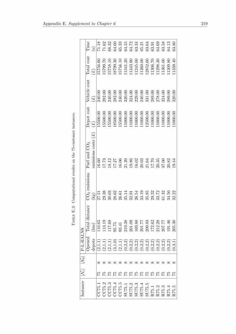
Appendix E. Supplement to Chapter 6 219
TableE.3:
Com
pu
tati
on
al
resu
lts
on
the
75-c
ust
om
erin
stan
ces.
Inst
an
ce|N
c||N
0|
P-L
-HA
LN
SO
pen
edT
ota
ld
ista
nce
CO
2em
issi
ons
Fu
elan
dC
O2
Dep
otco
stV
ehic
leco
stT
otal
cost
Tim
ed
epots
(km
)(k
g)em
issi
ons
cost
s(£
)(£
)(£
)(£
)(s
)
CC
751
758
(2,1
,1)
110.
6527
.51
16.6
015
500.
0024
0.00
1575
6.60
71.1
8C
C75
275
8(2
,1,1
)11
3.19
29.3
817
.73
1550
0.00
282.
0015
799.
7071
.62
CC
753
758
(2,1
,1)
117.
6830
.03
18.1
215
500.
0024
0.00
1575
8.10
68.3
2C
C75
475
8(3
,1,0
)95
.75
28.6
217
.27
1850
0.00
282.
0018
799.
3064
.60
CC
755
758
(2,1
,1)
93.4
126
.61
16.0
615
500.
0024
0.00
1575
6.10
65.3
3S
U75
175
8(0
,2,2
)21
9.38
35.1
421
.20
1100
0.00
320.
0011
341.
2064
.55
SU
752
758
(0,2
,2)
201.
0932
.91
19.8
611
000.
0032
4.00
1134
3.90
64.7
2S
U75
375
8(0
,2,2
)16
9.80
26.5
416
.02
1100
0.00
229.
0011
245.
0063
.34
SU
754
758
(0,2
,2)
201.
7733
.19
20.0
311
000.
0024
0.00
1126
0.00
65.2
1S
U75
575
8(0
,2,2
)20
9.93
35.8
521
.64
1250
0.00
331.
0012
852.
6063
.64
R75
175
8(0
,2,2
)17
2.62
29.3
217
.70
1100
0.00
289.
0011
306.
7063
.91
R75
275
8(0
,2,2
)21
2.28
33.7
220
.35
1100
0.00
278.
0011
298.
3064
.69
R75
375
8(0
,2,2
)20
7.77
61.3
237
.00
1100
0.00
324.
0011
361.
0063
.58
R75
475
8(0
,2,2
)19
1.46
34.5
020
.82
1100
0.00
289.
0011
309.
8064
.13
R75
575
8(0
,3,1
)20
5.30
32.2
219
.44
1100
0.00
320.
0011
339.
4063
.80

Appendix E. Supplement to Chapter 6 220
TableE.4:
Com
pu
tati
on
al
resu
lts
on
the
100-c
ust
om
erin
stan
ces.
Inst
an
ce|N
c||N
0|
P-L
-HA
LN
SO
pen
edT
ota
ld
ista
nce
CO
2em
issi
ons
Fu
elan
dC
O2
Dep
otco
stV
ehic
leco
stT
otal
cost
Tim
ed
epots
(km
)(k
g)em
issi
ons
cost
s(£
)(£
)(£
)(£
)(s
)
CC
100
110
010
(3,1
,2)
145.
5934
.20
20.6
422
500.
0034
9.00
2286
9.60
159.
53C
C10
02
100
10
(2,1
,2)
125.
5736
.64
22.1
117
500.
0034
2.00
1786
4.10
176.
07C
C10
03
100
10
(3,2
,0)
143.
7070
.06
42.2
722
000.
0039
1.00
2243
3.30
176.
89C
C10
04
100
10
(3,1
,2)
143.
1538
.26
23.0
922
500.
0036
0.00
2288
3.10
178.
28C
C10
05
100
10
(2,2
,1)
143.
2138
.88
23.4
619
000.
0034
9.00
1937
2.50
156.
76S
U10
01
100
10
(0,3
,3)
236.
5041
.44
25.0
114
500.
0038
4.00
1490
9.00
167.
88S
U10
02
100
10
(0,2
,3)
242.
5243
.71
26.3
814
500.
0042
6.00
1495
2.40
146.
06S
U10
03
100
10
(0,2
,3)
246.
5238
.64
23.3
214
500.
0043
3.00
1495
6.30
147.
51S
U10
04
100
10
(0,2
,3)
255.
2044
.68
26.9
616
500.
0036
0.00
1688
7.00
147.
15S
U10
05
100
10
(0,2
,3)
241.
4941
.61
25.1
114
500.
0038
4.00
1490
9.10
147.
17R
100
110
010
(0,3
,2)
250.
4710
6.86
64.4
814
500.
0038
0.00
1494
4.50
148.
83R
100
210
010
(0,3
,2)
262.
3343
.66
26.3
513
000.
0038
4.00
1341
0.30
147.
92R
100
310
010
(0,3
,2)
263.
7243
.55
26.2
813
000.
0039
8.00
1342
4.30
159.
90R
100
410
010
(0,3
,3)
257.
9042
.53
25.6
713
000.
0038
4.00
1340
9.70
157.
72R
100
510
010
(0,3
,2)
262.
7036
.68
22.1
314
500.
0043
3.00
1495
5.10
176.
27

Bibliography
Achuthan, N., Caccetta, L. and Hill, S. (2003), ‘An improved branch-and-cut algorithm for the
capacitated vehicle routing problem’, Transportation Science 37, 153–169.
Afshar-Nadjafi, B. and Afshar-Nadjafi, A. (2014), ‘A constructive heuristic for time-dependent
multi-depot vehicle routing problem with time-windows and heterogeneous fleet’, Journal
of King Saud University-Engineering Sciences, in press.
Ambrosino, D., Sciomachen, A. and Scutella, M. G. (2009), ‘A heuristic based on multiexchange
techniques for a regional fleet assignment location-routing problem’, Computers & Opera-
tions Research 36, 442–460.
Alba, E. and Dorronsoro, B. (2006), ‘Computing nine new best-so-far solutions for capacitated
VRP with a cellular genetic algorithm’, Information Processing Letters 98, 225–230.
Albareda-Sambola, M., Dıaz, J. A. and Fernandez, E. (2005), ‘A compact model and tight
bounds for a combined location-routing problem’, Computers & Operations Research 32,
407–428.
Albareda-Sambola, M. (2015), Location-routing and location-arc routing problems. In Laporte,
G., Nickel, S., Saldanha da Gama, F. (Eds.), Location Science. (pp. 399–418). Springer,
Berlin-Heidelberg.
Baldacci, R., Battarra, M. and Vigo, D. (2008), Routing a heterogeneous fleet of vehicles. In
Golden, B.L., Raghavan, S., Wasil, E.A. (Eds), The Vehicle Routing Problem: Latest
Advances and New Challenges. Springer, New York.
Baldacci, R. and Mingozzi, A. (2009), ‘A unified exact method for solving different classes of
vehicle routing problems’, Mathematical Programming 120, 347–380.
Baldacci, R., Battarra, M. and Vigo, D. (2009), ‘Valid inequalities for the fleet size and mix
vehicle routing problem with fixed costs’, Networks 54, 178–189.
Baldacci, R., Toth, P. and Vigo, D. (2010a), ‘Exact algorithms for routing problems under vehicle
capacity constraints’, Annals of Operations Research 175, 213–245.
Baldacci, R., Bartolini, E., Mingozzi, A. and Roberti, R. (2010b), ‘An exact solution framework
for a broad class of vehicle routing problems’, Computational Management Science 7, 229–
268.
221

Bibliography 222
Balinski, M. L. (1965), ‘Integer programming: Methods, uses, computation’, Management Sci-
ence 12, 253–313.
Barbarosoglu, G. and Ozgur, D. (1999), ‘A tabu search algorithm for the vehicle routing problem’,
Computers & Operations Research 26, 255–270.
Barreto, S. (2004), Analise e modelizacao de problemas de localizacao-distribuicao (Analysis
and modelling of location-routing problems). Ph.D. thesis, University of Aveiro, Aveiro,
Portugal.
Barth, M. and Boriboonsomsin, K. (2008), ‘Real-world CO2 impacts of traffic congestion’.
Technical report, Paper for the 87th Annual Meeting of Transportation Research Board.
<http://www.uctc.net/papers/846.pdf> (accessed 21.01.2014).
Barth, M. and Boriboonsomsin, K. (2009), ‘Energy and emissions impacts of a freeway-based
dynamic eco-driving system’, Transportation Research Part D: Transport and Environment
14, 400–410.
Barth, M., Younglove, T. and Scora, G. (2005), Development of a heavy-duty diesel modal
emissions and fuel consumption model. Technical report UCB-ITS-PRR-2005-1, California
PATH Program, Institute of transportation Studies, University of California at Berkeley.
Beasley, J. E. (1983), ‘Route first-cluster second methods for vehicle routing’, Omega 11, 403–
408.
Bektas, T. and Crainic, T. G. (2008), ‘Brief overview of intermodal transportation’,. In Taylor,
G. D. (Eds), Logistics Engineering Handbook. Boca Raton, CRC Press, New York.
Bektas, T. and Laporte, G. (2011), ‘The pollution-routing problem’, Transportation Research
Part B: Methodological 45, 1232–1250.
Bektas, T., Repoussis, P. P. and Tarantilis, C. D. (2014), Dynamic Vehicle Routing Problems.
In Toth, P., Vigo, D., (Eds.), Vehicle Routing: Problems, Methods, and Applications. (pp.
299–347). MOS-SIAM Series on Optimization, Philadelphia.
Belfiore, P. and Yoshizaki, H. T. Y. (2009), ‘Scatter search for a real-life heterogeneous fleet
vehicle routing problem with time windows and split deliveries in Brazil’, European Journal
of Operational Research 199, 750–758.
Belfiore, P. and Yoshizaki, H. T. Y. (2013), ‘Heuristic methods for the fleet size and mix ve-
hicle routing problem with time windows and split deliveries’, Computers & Industrial
Engineering 64, 589–601.
Belmecheri, F., Prins, C., Yalaoui, F. and Amodeo, L. (2013), ‘Particle swarm optimization
algorithm for a vehicle routing problem with heterogeneous fleet, mixed backhauls, and
time windows’, Journal of Intelligent Manufacturing 24, 775–789.
Berger, R. T., Coullard, C. R. and Daskin, M. S. (2007), ‘Location-routing problems with dis-
tance constraints’, Transportation Science 41, 29–43.

Bibliography 223
Bettinelli, A., Ceselli, A. and Righini, G. (2011), ‘A branch-and-cut-and-price algorithm for the
multi-depot heterogeneous vehicle routing problem with time windows’, Transportation
Research Part C: Emerging Technologies 19, 723–740.
Bettinelli, A., Ceselli, A. and Righini, G. (2014), ‘A branch-and-price algorithm for the multi-
depot heterogeneous-fleet pickup and delivery problem with soft time windows’, Mathe-
matical Programming Computation 6, 171–197.
Bigazzi, A. Y. and Figliozzi, M. A. (2012), Congestion and emissions mitigation: A comparison of
capacity, demand, and vehicle based strategies. Transportation Research Part D: Transport
and Environment 17, 538–547.
Birge, J. R. and Louveaux, F. (2011), Introduction to Stochastic Programming. Springer, New
York.
Bolduc, M.-C., Renaud, J. and Montreuil, B. (2006), ‘Synchronized routing of seasonal prod-
ucts through a production/distribution network’, Central European Journal of Operations
Research 14, 209–228.
Bolduc, M.-C., Renaud, J. and Boctor, F. (2007), ‘A heuristic for the routing and carrier selection
problem’, European Journal of Operational Research 183, 926–932.
Bolduc, M.-C., Renaud, J., Boctor, F. and Laporte, G. (2008), ‘A perturbation metaheuristic
for the vehicle routing problem with private fleet and common carriers’, Journal of the
Operational Research Society 59, 776–787.
Boudoin, D., Morel, C. and Gardat, M. (2014), Supply chains and urban logistics platforms. In
Gonzalez-Feliu, J., Semet, F., Routhier, J.-L., (Eds.). Sustainable Urban Logistics: Con-
cepts, Methods and Information Systems. (pp. 1–20). Springer, Berlin-Heidelberg.
Brandao, J. (2009), ‘A deterministic tabu search algorithm for the fleet size and mix vehicle
routing problem’, European Journal of Operational Research 195, 716–728.
Brandao, J. (2011), ‘A tabu search algorithm for the heterogeneous fixed fleet vehicle routing
problem’, Computers & Operations Research 38, 140–151.
Braysy, O., Dullaert, W., Hasle, G., Mester, D. and Gendreau, M. (2008), ‘An effective mul-
tirestart deterministic annealing metaheuristic for the fleet size and mix vehicle routing
problem with time windows’, Transportation Science 42, 371–386.
Braysy, O., Porkka, P. P., Dullaert, W., Repoussis, P. P. and Tarantilis, C. D. (2009), ‘A well
scalable metaheuristic for the fleet size and mix vehicle-routing problem with time windows’,
Expert System with Applications 36, 8460–8475.
Calvete, H. I., Gale, C, Oliveros, M-J. and Sanchez-Valverde, B. (2007), ‘A goal programming
approach to vehicle routing problems with soft time windows’, European Journal of Oper-
ational Research 177, 1720–1733.

Bibliography 224
Campbell, J.F. (1995a), ‘Peak period large truck restrictions and a shift to off-peak operations:
Impact on truck emissions and performance’, Journal of Business Logistics 16, 227–248.
Campbell, J.F. (1995b), ‘Using small trucks to circumvent large truck restrictions: impacts on
truck emissions and performance measures’, Transportation Research Part A: Policy and
Practice 29, 445–458.
Caterpillar. (2006), Tractor-trailer performance guide, Technical report <http://www.cat.com/
cda/files/2222280/> (accessed 01.02.2014).
Ceschia, S., Luca Di, G. and Andrea, S. (2011), ‘Tabu search techniques for the heteroge-
neous vehicle routing problem with time windows and carrier-dependent costs’, Journal of
Scheduling 14, 601–615.
Chao, I-M., Golden, B. L and Wasil, E. A. (1999), ‘A computational study of a new heuristic
for the site-dependent vehicle routing problem’, INFOR 37, 319–336.
Choi, E. and Tcha, D. W. (2007), ‘A column generation approach to the heterogeneous fleet
vehicle routing problem’, Computers & Operations Research 34, 2080–2095.
Christofides, N. and Eilon, S. (1969), ‘An algorithm for the vehicle dispatching problem’, Oper-
ational Research Quarterly 20, 309–318.
Chu, C. W. (2005), ‘A heuristic algorithm for the truckload and less-than-truckload problem’,
European Journal of Operational Research 165, 657–667.
Clarke, G. and Wright, J. W. (1964), ‘Scheduling of vehicles from a central depot to a number
of delivery points’, Operations Research 12, 568–581.
Coe, E. (2005), Average carbon dioxide emissions resulting from gasoline and diesel fuel. United
States Environmental Protection Agency, Technical report <http://www.epa.gov/otaq/
climate/420f05001.pdf> (accessed 11.02.2014).
Cordeau, J-F., Laporte, G. and Mercier, A. (2001), ‘A unified tabu search heuristic for vehicle
routing problems with time windows’, Journal of the Operational Research Society 52,
928–936.
Cordeau, J.-F., Laporte, G., Savelsbergh, M. W. P. and Vigo, D. (2007), Vehicle routing. In:
Barnhart, C. and Laporte, G. (Eds.), Transportation, Handbooks in Operations Research
and Management Science. Elsevier, Amsterdam.
Cormen, T. H., Stein, C., Rivest, R. L. and Leiserson, C. E. (2001). Introduction to Algorithms.
McGraw-Hill Higher Education.
Crainic, T. G. and Laporte, G. (1997). Planning models for freight transportation. European
Journal of Operational Research 97, 409–438.
Dablanc, L. (2014), Logistics sprawl and urban freight planning issues in a major gateway city.
In Gonzalez-Feliu, J., Semet, F., Routhier, J.-L., (Eds.). Sustainable Urban Logistics: Con-
cepts, Methods and Information Systems. (pp. 49–69). Springer, Berlin-Heidelberg.

Bibliography 225
Daganzo, C.F., (1984a), ‘The distance traveled to visit N points with a maximum of C stops per
vehicle’, Transportation Science 18, 135–146.
Daganzo, C.F., (1984b), ‘The length of tours in zones of different shapes’, Transportation Re-
search Part B: Methodological 18, 135–146.
Dantzig, G. B. and Ramser, J. H. (1959), ‘The truck dispatching problem’, Management Science
6, 80–91.
Dantzig, G. B., Fulkerson, D. R. and Johnson, S. M. (1954), ‘Solution of a large-scale traveling
salesman problem’, Operations Research 2, 393–410.
Dayarian, I., Crainic, T. G., Gendreau, M. and Rei, W. (2015). ‘A column generation approach
for a multi-attribute vehicle routing problem’. European Journal of Operational Research
241, 888–906.
DEFRA. (2007), Effects on payload on the fuel consumption of
trucks, Technical report, <http://www.freightbestpractice.org.uk/
effects-of-payload-on-fuel-consumption-of-trucks> (accessed 15.02.2014).
DEFRA. (2012), Guidelines to DEFRA/ DECC’s GHG conversion factors for company
reporting: Methodology paper for emission factors, Technical report London, United King-
dom. <https://www.gov.uk/government/uploads/system/uploads/attachment_data/
file/69568/pb13792-emission-factor-methodology-paper-120706.pdf> (accessed
17.02.2014).
De la Cruz, J. J., Paternina-Arboleda, C. D., Cantillo, V. and Montoya-Torres, J. R. (2013),
‘A two-pheromone trail ant colony system—tabu search approach for the heterogeneous
vehicle routing problem with time windows and multiple products’, Journal of Heuristics
19, 233–252.
Dell’Amico, M., Monaci, M., Pagani, C. and Vigo. D. (2007), ‘Heuristic approaches for the
fleet size and mix vehicle routing problem with time windows’, Transportation Science 41,
516–526.
Demir, E., Bektas, T. and Laporte, G. (2011), ‘A comparative analysis of several vehicle emission
models for road freight transportation’, Transportation Research Part D: Transport and
Environment 6, 347–357.
Demir, E., Bektas, T. and Laporte, G. (2012), ‘An adaptive large neighborhood search heuristic
for the pollution-routing problem’, European Journal of Operational Research 223, 346–
359.
Demir, E., Bektas, T. and Laporte, G. (2014a), ‘The bi-objective pollution-routing problem’,
European Journal of Operational Research 232, 464–478.
Demir, E., Bektas, T. and Laporte, G. (2014b), ‘A review of recent research on green road freight
transportation’, European Journal of Operational Research 237, 775–793.

Bibliography 226
Desrochers, M. and Verhoog, T. W. (1991), ‘A new heuristic for the fleet size and mix vehicle
routing problem’, Computers & Operations Research 18, 263–274.
DfT. (2010), Truck specification for best operational efficiency, United Kingdom Department
for Transport, United Kingdom. <http://www.freightbestpractice.org.uk/download.
aspx?pid=124> (accessed 10.02.2014).
DfT. (2012), Reducing greenhouse gases and other emissions from transport. United King-
dom Department for Transport, United Kingdom. <http://www.gov.uk/government/
policies/reducing-greenhouse-gases-and-other-emissions-from-transport> (ac-
cessed 15.02.2014).
DfT. (2013), Setting local speed limits. United Kingdom Department for Trans-
port. <https://www.gov.uk/government/uploads/system/uploads/attachment_data/
file/63975/circular-01-2013.pdf> (accessed 10.12.2014).
Dijkstra, E., (1959), A note on two problems in connexion with graphs. Numerische Mathematik
1, 269–271.
Dominguez, O., Juan, A. A., Barrios, B., Faulin, J. and Agustin, A. (2014). Using biased random-
ization for solving the two-dimensional loading vehicle routing problem with heterogeneous
fleet. Annals of Operations Research, 1–22.
Dondo, R. and Cerda, J. (2007), ‘A cluster-based optimization approach for the multi-depot
heterogeneous fleet vehicle routing problem with time windows’, European Journal of Op-
erational Research 176, 1478–1507.
Drexl, M. and Schneider, M., (2015). ‘A survey of variants and extensions of the location-routing
problem’, European Journal of Operational Research 241, 283–308.
Dueck, G. (1993), ‘New optimization heuristics: The great deluge algorithm and the record-to-
record travel’, Journal of Computational Physics 104, 86–92.
Duhamel, C., Lacomme, P., Prins, C. and Prodhon, C. (2010), ‘A GRASPXELS approach for the
capacitated location-routing problem’, Computers & Operations Research 37, 1912–1923.
Duhamel, C., Lacomme, P. and Prodhon, C. (2011), ‘Efficient frameworks for greedy split and
new depth first search split procedures for routing problems’, Computers & Operations
Research 38, 723–739.
Duhamel, C., Lacomme, P. and Prodhon, C. (2012), ‘A hybrid evolutionary local search with
depth first search split procedure for the heterogeneous vehicle routing problems’, Engi-
neering Applications of Artificial Intelligence 25, 345–358.
Dullaert, W., Janssens, G. K., Sorensen, K. and Vernimmen, B. (2002), ‘New heuristics for the
fleet size and mix vehicle routing problem with time windows’, Journal of the Operational
Research Society 53, 1232–1238.
<http://www.gov.uk/government/policies/reducing-greenhouse-gases-and-other-emissions-from-transport>

Bibliography 227
Eglese, R. and Bektas, T. (2014). Green vehicle routing. In Toth, P., Vigo, D., (Eds.), Vehi-
cle Routing: Problems, Methods, and Applications. (pp. 437–458). MOS-SIAM Series on
Optimization, Philadelphia.
Ehmke, J. F., Campbell, A. M. and Thomas, B. W., (2014), Solution approaches for stochastic
emissions-minimized paths in urban areas. Technical report, University of Iowa, Iowa City.
EPA. (2010), Greenhouse Gas Emissions Model (GEM) User Guide. United States Environ-
mental Protection Agency, USA. <http://www.epa.gov/otaq/climate/regulations/
420b10039.pdf> (accessed 18.02.2014).
EPA. (2012), DRAFT inventory of United States greenhouse gas emissions and sinks: 1990-
2012. United States Environmental Protection Agency, USA. <http://www.epa.gov/
climatechange/Downloads/ghgemissions/US-GHG-Inventory-2014-Main-Text.pdf>
(accessed 15.02.2014).
Euchi, J. and Chabchoub, H. (2010), ‘A hybrid tabu search to solve the heterogeneous fixed fleet
vehicle routing problem’, Logistics Research 2, 3–11.
Fagerholt, K., Laporte, G. and Norstad, I. (2010), Reducing fuel emissions by optimizing speed
on shipping routes. Journal of the Operational Research Society 61, 523–529.
FedEx. (2015), <http://www.fedex.com/gb/about/index.html> (accessed 10.01.2015).
Ferland, J. A. and Michelon, P. (1988), ‘The vehicle scheduling problem with multiple vehicle
types’, Journal of the Operational Research Society 39, 577–583.
FHWA. (2011), Vehicle Types. United States Department of Transport, FederaL Highway Ad-
ministration, USA. <http://www.fhwa.dot.gov/policy/ohpi/vehclass.htm> (accessed
25.02.2014).
Figliozzi, M. A. (2011), The impact of congestion on time-definitive urban freight distribution
networks CO2 emission levels: Results from a case study in Portland, Oregon. Transporta-
tion Research Part C: Emerging Technologies 19, 766–778.
Fisher, M. L. and Jaikumar, R. (1981), ‘A generalized assignment heuristic for vehicle routing’,
Networks 11, 109–124.
Franceschelli, M., Rosa, D., Seatzu, C. and Bullo, F. (2013), ‘Gossip algorithms for heterogeneous
multi-vehicle routing problems’, Nonlinear Analysis: Hybrid Systems 10, 156–174.
Franceschetti, A., Honhon, D., Van Woensel, T., Bektas, T. and Laporte, G. (2013), ‘The time-
dependent pollution-routing problem’, Transportation Research Part B: Methodological 56,
265–293.
Geisberger, R., Sanders, P., Schultes, D. and Vetter, C. (2012), Exact routing in large road
networks using contraction hierarchies. Transportation Science 46, 388–404.

Bibliography 228
Gencer, C., Top, I. and Aydogan, E. K. (2006), ‘A new intuitional algorithm for solving hetero-
geneous fixed fleet routing problems: Passenger pickup algorithm’, Applied Mathematics
and Computation 181, 1552–1567.
Gendreau, M., Hertz, A. and Laporte, G. (1992), ‘New insertion and postoptimization procedures
for the travelling salesman problem’, Operations Research 40, 1086–1094.
Gendreau, M., Laporte, G., Musaraganyi, C. and Taillard, E. D. (1999), ‘A tabu search heuristic
for the heterogeneous fleet vehicle routing problem’, Computers & Operations Research 26,
1153–1173.
Gendreau, M., Iori, M., Laporte, G. and Martello, S. (2008), ‘A tabu search heuristic for the
vehicle routing problem with two-dimensional loading constraints’, Networks 51, 4–18.
Gheysens, F., Golden, B. L. and Assad, A. A. (1984), ‘A comparison of techniques for solving
the fleet size and mix vehicle routing problem’, OR Spektrum 6, 207–216.
Gheysens, F., Golden, B. L. and Assad, A. A. (1986), ‘A new heuristic for determining fleet size
and composition’, Mathematical Programming Study 26, 233–236.
Ghiani, G., Laporte, G. and Musmanno, R. (2013). Introduction to Logistics Systems Manage-
ment. Wiley, Chichester.
Golden, B. L., Assad, A.A., Levy, L. and Gheysens, F. (1984), ‘The fleet size and mix vehicle
routing problem’, Computers & Operations Research 11, 49–66.
Golden, B. L., Raghavan S. and Wasil E. A. (2008), The vehicle routing problem: Latest advances
and new challenges. Springer, New York.
Gonzalez-Feliu, J., Semet, F. and Routhier, J.-L. (Eds.) (2014), Sustainable Urban Logistics:
Concepts, Methods and Information Systems. Springer, Berlin-Heidelberg.
Google Maps. (2015), <https://maps.google.com> (accessed 15.01.2015).
Green Logistics. (2014), What is green logistics?, Cardiff, UK. <http://www.greenlogistics.
org/>.
Han, A. F.-W. and Cho, Y.-J. (2002), A GIDS metaheuristic approach to the fleet size and
mix vehicle routing problem. In: Ribeiro, C.C., Hansen, P., editors. Essays and surveys in
metaheuristics. (pp. 399–413). Kluwer Academic Publishers, Boston.
Hemmelmayr, V. C., Cordeau, J-F. and Crainic, T. G. (2012), ‘An adaptive large neighborhood
search heuristic for two-echelon vehicle routing problems arising in city logistics’, Computers
& Operations Research 39, 3215–3228.
Ho, S. C. and Haugland, D. (2004), ‘A tabu search heuristic for the vehicle routing problem with
time windows and split deliveries’, Computers & Operations Research 31, 1947–1964.
Hoff, A. and Andersson, H., Christiansen, M., Hasle, G. and Løkketangen, A. (2010), ‘Industrial
aspects and literature survey: Fleet composition and routing’, Computers & Operations
Research 37, 2041–2061.

Bibliography 229
Holland, J. H. (1975), ‘Adaptation in natural and artificial systems. an introductory analysis
with applications to biology, control and artificial intelligence’, Ann Arbor: The University
of Michigan Press, Michigan.
Homberger, J. and Gehring, H. (1999), ‘Two evolutionary metaheuristics for the vehicle routing
problem with time windows’, INFOR, Information Systems and Operational Research 3,
297–318.
Hvattum, L. M., Norstad, I., Fagerholt, K. and Laporte, G. (2013), ‘Analysis of an exact algo-
rithm for the vessel speed optimization problem’, Networks 62, 132–135.
Imran, A., Salhi, S. and Wassan, N. A. (2009), ‘A variable neighborhood-based heuristic for the
heterogeneous fleet vehicle routing problem’, European Journal of Operational Research
197, 509–518.
Imran, A., Salhi, S. and Wassan, N. A. (2009), ‘A variable neighborhood-based heuristic for the
heterogeneous fleet vehicle routing problem’, European Journal of Operational Research
197, 509–518.
Iori, M., Salazar, J. J. and Vigo, D. (2007), ‘An exact approach for the vehicle routing problem
with two dimensional loading constraints’, Transportation Science 41, 253–264.
Iori, M. and Riera-Ledesma, J. 2015. ‘Exact algorithms for the double vehicle routing problem
with multiple stacks’. Computers & Operations Research 63, 83–101.
Irnich, S. (2000), ‘A multi-depot pick up and delivery problem with a single hub and heteroge-
neous vehicles’, European Journal of Operational Research 122, 310–328.
Irnich, S., Schneider, M. and Vigo, D. (2014), Four variants of the vehicle routing problem, in
P. Toth and D. Vigo, (Eds.), Vehicle Routing: Problems, Methods and Applications. (pp.
241–271). MOS-SIAM Series in Optimization, Philadelphia.
Jabali, O., Gendreau, M. and Laporte, G. (2012a), ‘A continuous approximation model for the
fleet composition problem’, Transportation Research Part B: Methodological 46, 1591–1606.
Jabali, O., Van Woensel, T. and de Kok, A.G. (2012b), ‘Analysis of travel times and CO2
emissions in time-dependent vehicle routing’, Production and Operations Management 21,
1060–1074.
Jiang, J., Ng, K. M., Poh, K. L. and Teo, K. M. (2014), ‘Vehicle routing problem with a
heterogeneous fleet and time windows’, Expert Systems with Applications 41, 3748–3760.
Juan, A. A., Goentzel, J. and Bektas, T. (2014), ‘Routing fleets with multiple driving ranges: Is
it possible to use greener fleet configurations?’, Applied Soft Computing 21, 84–94.
Kahn Ribeiro, S., Kobayashi, S., Beuthe, M., Gasca, J., Greene, D., Lee, D.S., Muromachi,
Y., Newton, P. J., Plotkin, S., Sperling, D., Wit, R. and Zhou, P.J. (2007), Transport
and its infrastructure. In Climate Change 2007: Mitigation. <http://www.ipcc.ch/pdf/
assessment-report/ar4/wg3/ar4-wg3-chapter5.pdf> (accessed 27.02.2014).

Bibliography 230
Karaoglan, I., Altiparmak, F., Kara, I. and Dengiz, B. (2011), A branch and cut algorithm for
the location-routing problem with simultaneous pickup and delivery, European Journal of
Operational Research 211, 318–332.
Karaoglan, I., Altiparmak, F., Kara, I. and Dengiz, B. (2012), ‘The location-routing problem
with simultaneous pickup and delivery: Formulations and a heuristic approach’, Omega
40, 465–477.
Kirby, H. R., Hutton, B., McQuaid, R. W., Raeside, R. and Zhang, X. (2000), ‘Modelling
the effects of transport policy levers on fuel efficiency and national fuel consumption’,
Transportation Research Part D: Transport and Environment 5, 265–282.
Kirkby, T. (2002), Memorandum by Kingston upon Hull City Council (RTS 152)- 20 mph
zones in Kingston upon Hull, Select Committee on Transport, Local Government and the
Regions, <http://www.publications.parliament.uk/pa/cm200102/cmselect/cmtlgr/
557/557ap80.htm> (accessed 9.12.2014).
Knorr, W. (2008), EcoTransIT: ecological transport information tool – environmental method-
ology and data, Technical Report. Institut fur Energie und Umweldforschung Heidelberg.
Koc, C., Bektas, T., Jabali, O. and Laporte, G. (2014), ‘The fleet size and mix pollution-routing
problem’, Transportation Research Part B: Methodological 70, 239–254.
Koc, C., Bektas, T., Jabali, O. and Laporte, G. (2015), ‘A hybrid evolutionary algorithm for
heterogeneous fleet vehicle routing problems’, Computers & Operations Research 64, 11–27.
Koc, C., Bektas, T., Jabali, O. and Laporte, G. (2016), ‘The fleet size and mix location-routing
problem with time windows: Formulations and a heuristic algorithm’, European Journal of
Operational Research 248, 33–51.
Kopfer, H. W. and Kopfer, H. (2013), Emissions minimization vehicle routing problem in de-
pendence of different vehicle classes. Kreowski, H-J., Reiter, B. S., Thoben, K-D. (Eds).
Dynamics in Logistics, Lecture Notes in Logistics. (pp. 49–58). Springer, Berlin.
Kopfer, H. W., Schonberger, J and Kopfer, H. (2014), ‘Reducing greenhouse gas emissions of a
heterogeneous vehicle fleet’, Flexible Services and Manufacturing Journal 26, 221–248.
Kramer, R., Subramanian, A., Vidal, T. and Lucıdio dos Anjos, F. C. (2015), A matheuristic
approach for the pollution-routing problem. European Journal of Operational Research
243, 523–539.
Krause, E. F. (2012), Taxicab geometry: An adventure in non-Euclidean geometry. Dover Pub-
lications, New York.
Kritikos, M. N. and Ioannou, G. (2013), ‘The heterogeneous fleet vehicle routing problem with
overloads and time windows’, International Journal of Production Economics 144, 68–75.

Bibliography 231
Kwon, Y. J., Choi, Y. J. and Lee, D. H. (2013), ‘Heterogeneous fixed fleet vehicle routing
considering carbon emission’, Transportation Research Part D: Transport and Environment
23, 81–89.
Lai, M., Crainic, T. G., Di Francesco, M. and Zuddas, P. (2013), ‘An heuristic search for the
routing of heterogeneous trucks with single and double container loads’, Transportation
Research Part E: Logistics and Transportation Review 56, 108–118.
Labbe, M., Rodrıguez-Martin, I. and Salazar-Gonzalez, J. J. (2004), ‘A branch-and-cut algorithm
for the plant-cycle location problem’, Journal of the Operational Research Society 55, 513–
520.
Laporte, G. (1988), Location-routing problems. In: Golden, B. L., Assad, A. A. (Eds.), Vehicle
Routing: Methods and Studies. North-Holland, Amsterdam.
Laporte, G. (2009), ‘Fifty years of vehicle routing’, Transportation Science 43, 408–416.
Laporte, G., Ropke, S. and Vidal, T. (2014), Heuristics for the vehicle routing problem, in
P. Toth and D. Vigo, eds., Vehicle Routing: Problems, Methods and Applications. (pp.
87–116). MOS-SIAM Series in Optimization, Philadelphia.
Laporte, G., Nickel, S. and Saldanha da Gama, F. (Eds.) (2015), Location Science. Springer,
Berlin-Heidelberg.
Lau, H. C., Sim, M. and Teo, K. M. (2003), ‘Vehicle routing problem with time windows and a
limited number of vehicles’, European Journal of Operational Research 148, 559–569.
Lee, Y. H., Kim, J. I., Kang, K. H. and Kim, K. H. (2008), ‘A heuristic for vehicle fleet mix
problem using tabu search and set partitioning’, Journal of the Operational Research Society
59, 833–841.
Leung, S. C. H., Zheng, J. M., Zhang, D. F. and Zhou, X. Y. (2010), ‘Metaheuristics for the
vehicle routing problem with two-dimensional loading constraints’, Flexible Services and
Manufacturing Journal 22, 61–82.
Leung, S. C., Zhang, Z., Zhang, D., Hua, X. and Lim, M. K. (2013), ‘A meta-heuristic algorithm
for heterogeneous fleet vehicle routing problems with two-dimensional loading constraints’,
European Journal of Operational Research 225, 199–210.
Levy, D., Sundar, K. and Rathinam, S. (2014), ‘Heuristics for routing heterogeneous unmanned
vehicles with fuel constraints’, Mathematical Problems in Engineering 2014, 1–12.
Li. F, Golden, B. L. and Wasil, E. A. (2005), ‘Very large-scale vehicle routing: new test problems,
algorithms and results’, Computers & Operations Research 32, 1165–1179.
Li, F., Golden, B. L. and Wasil, E. A. (2007), ‘A record-to-record travel algorithm for solving
the heterogeneous fleet vehicle routing problem’, Computers & Operations Research 34,
2734–2742.

Bibliography 232
Li, X., Tian, P. and Aneja, Y. P. (2010), ‘An adaptive memory programming metaheuristic for
the heterogeneous fixed fleet vehicle routing problem’, Transportation Research Part E:
Logistics and Transportation Review 46, 1111–1127.
Li, X., Leung, S. C. and Tian, P. (2012), ‘A multistart adaptive memory-based tabu search
algorithm for the heterogeneous fixed fleet open vehicle routing problem’, Expert Systems
with Applications 39, 365–374.
Lima, C. D. R., Goldbarg, M. C. and Goldbarg, E. F. G. (2004), ‘A memetic algorithm for the
heterogeneous fleet vehicle routing problem’, Electronic Notes in Discrete Mathematics 18,
171–176.
Lin, C., Choy, K. L., Ho, G. T. S., Chung, S. H. and Lam, H. Y. (2014), ‘Survey of Green
Vehicle Routing Problem: Past and future trends’, Expert Systems with Applications 41,
1118–1138.
Liu, S. (2013), ‘A hybrid population heuristic for the heterogeneous vehicle routing problems’,
Transportation Research Part E: Logistics and Transportation Review 54, 67–78.
Liu, S., Huang, W. and Ma, H. (2009), ‘An effective genetic algorithm for the fleet size and mix
vehicle routing problems’, Transportation Research Part E: Logistics and Transportation
Review 45, 434–445.
Liu, F. H. and Shen, S. Y. (1999a), ‘A method for vehicle routing problem with multiple vehicle
types and times windows’, Proceedings of the National Science Council, Republic of China,
Part A: Physical Science and Engineering 23 526–536.
Liu, F. H., and Shen, S. Y. (1999b), ‘The fleet size and mix vehicle routing problem with time
windows’, Journal of the Operational Research Society 50, 721–732.
Maden, W., Eglese, R. and Black, D. (2010), Vehicle routing and scheduling with time-varying
data: A case study. Journal of the Operational Research Society 61, 515–522.
MAN. (2014a), Trucks in distribution transport. <http://www.mantruckandbus.co.uk/en/
trucks/start_trucks.html> (accessed 26.02.2014).
MAN Engines. (2014b), <http://www.engines.man.eu/global/en/index.html#7906576>
(accessed 05.08.2014).
MAN Spec Sheets. (2014c), <http://www.man-bodybuilder.co.uk/specs/euro6/> (accessed
05.08.2014).
MAN, 2015a. Trucks in distribution transport. <http://www.mantruckandbus.co.uk/en/
trucks/start_trucks.html> (accessed 19.01.2015).
MAN Engines, 2015b. <http://www.engines.man.eu/global/en/index.html#7906576> (ac-
cessed 19.01.2015).
MAN Spec Sheets. 2015c. <http://www.man-bodybuilder.co.uk/specs/euro6/> (accessed
19.01.2015).
Bibliography 233
Mancini, S., Gonzalez-Feliu, J. and Crainic, T. G. (2014), Planning and optimization methods
for advanced urban logistics systems at tactical level. In Gonzalez-Feliu, J., Semet, F. and
Routhier, J.-L., (Eds.). Sustainable Urban Logistics: Concepts, Methods and Information
Systems. (pp. 145–164). Springer, Berlin-Heidelberg.
Maranzana, F. (1964), ‘On the location of supply points to minimize transport costs’, Operational
Research Quarterly 15, 261–270.
McKinnon, A. (2007), ‘CO2 Emissions from freight transport in the UK’. Technical Re-
port. Prepared for the Climate Change Working Group of the Commission for
Integrated Transport, London, UK. <www.isotrak.com/news/press/CO2_emissions_
freight_transport.pdf> (accessed on October 25, 2012).
Mercedes-Benz. (2014), Distribution. <http://www2.mercedes-benz.co.uk/content/
unitedkingdom/mpc/mpc_unitedkingdom_website/en/home_mpc/truck/home/new_
trucks/showroom.flash.html> (accessed 24.03.2014).
Miller, C. E., Tucker, A. W. and Zemlin, R. A. (1960), ‘Integer programming formulations
and traveling salesman problems’, Journal of the Association for Computing Machinery 7,
326–329.
Min, H., Jayaraman, V. and Srivastava, R. (1998), ‘Combined location-routing problems: A
synthesis and future research directions’, European Journal of Operational Research 108,
1–15.
Moscato, P. (1989), ‘On Evolution, Search, Optimization, Genetic Algorithms and Martial
Arts: Towards Memetic Algorithms’, Techical report, California Institute of Technology,
Pasadena CA, USA.
Moscato, P. and Cotta, C. (2010), ‘A Modern Introduction to Memetic Algorithms’. M. Gen-
dreau, J.-Y. Potvin, eds., Handbook of Metaheuristics (pp. 141–183). Springer, Boston.
Moutaoukil, A., Neubert, G. and Derrouiche, R. (2014), A comparison of homogeneous and
heterogeneous vehicle fleet size in green vehicle routing problem. In Advances in Produc-
tion Management Systems. Innovative and Knowledge-Based Production Management in
a Global-Local World (pp. 450–457). Springer, Berlin Heidelberg.
Muhlenbein, H., Gorges-Schleuter, M. and O. Kramer. (1988), ‘Evolution algorithms in combi-
natorial optimization’, Parallel Computing 7, 65–85.
Nag, B., Golden, B. L. and Assad, A. A. (1988), Vehicle routing with site dependencies. In B.L.
Golden and A. Assad, eds, Vehicle Routing: Methods and Studies. (pp 149–159). Elsevier,
Amsterdam.
Nagata, Y., Braysy, O. and Dullaert, W. (2010), ‘A penalty-based edge assembly memetic al-
gorithm for the vehicle routing problem with time windows’, Computers & Operations
Research 37, 724–737.

Bibliography 234
Nagy, G. and Salhi, S. (2007), ‘Location-routing: Issues, models and methods’, European Journal
of Operational Research 177, 649–672.
Naji-Azimi, Z. and Salari, M. (2013), ‘A complementary tool to enhance the effectiveness of ex-
isting methods for heterogeneous fixed fleet vehicle routing problem’, Applied Mathematical
Modelling 37, 4316–4324.
Newell, G.F. and Daganzo, C.F., (1986), ‘Design of multiple-vehicle delivery tours – I: A ring-
radial network’, Transportation Research Part B: Methodological 20, 345–363.
Norstad, I., Fagerholt, K. and Laporte, G. (2010), ‘Tramp ship routing and scheduling with
speed optimization’, Transportation Research Part C: Emerging Technologies 19, 853–865.
Ochi, L. S., Vianna, D. S., Drummond, L. M. and Victor, A. O. (1998a), A parallel evolution-
ary algorithm for the vehicle routing problem with heterogeneous fleet. In Parallel and
Distributed Processing. (pp. 216–224). Springer, Berlin Heidelberg.
Ochi, L. S., Vianna, D. S., Drummond, L. M. and Victor, A. O. (1998b), An evolutionary hybrid
metaheuristic for solving the vehicle routing problem with heterogeneous fleet. In Genetic
Programming (pp. 187–195). Springer, Berlin Heidelberg.
Or, I. (1976), Traveling salesman-type combinatorial problems and their relation to the logistics
of regional blood banking. PhD thesis, Department of Industrial Engineering and Manage-
ment Sciences, Northwestern University, Evanston, IL.
Oregon Department of Transportation. (2015a), Speed zoning program. <http://www.
oregon.gov/ODOT/HWY/TRAFFIC-ROADWAY/pages/speed_zone_program.aspx> (accessed
23.01.2015).
Oregon Department of Transportation. (2015b), Setting speeds. <http://www.oregon.gov/
ODOT/HWY/TRAFFIC-ROADWAY/docs/pdf/speed_final.pdf> (accessed 23.01.2015).
Osman, I. H. (1993), ‘Metastrategy simulated annealing and tabu search algorithms for the
vehicle routing problem’, Annals of Operations Research 41, 421–451.
Osman, I. H. and Salhi, S. (1996), Local search strategies for the vehicle fleet mix problem. In:
Rayward-Smith, V. J. , Osman I. H., Reeves, C. R., Smith, G.D., editors. Modern heuristic
search methods. (pp. 131–154). John Wiley, Chichester.
Ottawa Transportation Committee. (2009), Speed zoning policy. <http://ottawa.ca/
calendar/ottawa/citycouncil/trc/2009/10-07/ACS2009-COS-PWS-0021.htm> (ac-
cessed 25.01.2015).
Paraskevopoulos, D. C., Repoussis, P. P., Tarantilis, C. D., Ioannou, G. and Prastacos, G. P.
(2008), ‘A reactive variable neighbourhood tabu search for the heterogeneous fleet vehicle
routing problem with time windows’, Journal of Heuristics 14, 425–455.
Penna, P. H. V., Subramanian, A. and Ochi, L. S. (2013), ‘An iterated local search heuristic for
the heterogeneous fleet vehicle routing problem’, Journal of Heuristics 19, 201–232.

Bibliography 235
Pessoa, A., Uchoa, E. and Poggi de Aragao, M. (2009), ‘A robust branch-cut-and-price algorithm
for the heterogeneous fleet vehicle routing problem’, Networks 54, 167–177.
Pisinger, D. and Ropke, S. (2007), ‘A general heuristic for vehicle routing problems’, Computers
& Operations Research 34, 2403–2435.
Potvin, J.-Y. and Naud, M. A. (2011), ‘Tabu search with ejection chains for the vehicle routing
problem with private fleet and common carrier’, Journal of the Operational Research Society
62, 326–336.
Prieto, A., Bellas, F., Caamano, P. and Duro, R. J. (2011), ‘Solving a heterogeneous fleet
vehicle routing problem with time windows through the asynchronous situated Coevolution
algorithm’. In Advances in Artificial Life. Darwin Meets von Neumann (pp. 200–207).
Springer, Berlin Heidelberg.
Prins, C. (2002), ‘Efficient heuristics for the heterogeneous fleet multitrip VRP with application
to a large-scale real case’, Journal of Mathematical Modelling and Algorithms 1, 135–150.
Prins, C. (2004), ‘A simple and effective evolutionary algorithm for the vehicle routing problem’,
Computers & Operations Research 31, 1985–2002.
Prins, C. (2009), ‘Two memetic algorithms for heterogeneous fleet vehicle routing problems’,
Engineering Applications of Artificial Intelligence 22, 916–928.
Prins, C., Prodhon, C. and Wolfler-Calvo, R. (2006a), ‘Solving the capacitated locationrouting
problem by a GRASP complemented by a learning process and a path relinking’, 4OR: A
Quarterly Journal of Operations Research 4, 221–238.
Prins, C., Prodhon, C. and Wolfler-Calvo, R. (2006b), ‘A memetic algorithm with population
management (MAj,PM) for the capacitated location-routing problem’. In J. Gottlieb & G.
R. Raidl (Eds.), Evolutionary computation in combinatorial optimization. Lecture notes in
computer science. (pp. 183–194). Berlin Heidelberg: Springer.
Prins, C. (2009), ‘Two memetic algorithms for heterogeneous fleet vehicle routing problems’,
Engineering Applications of Artificial Intelligence 22, 916–928.
Prodhon, C. (2006), Le Probleme de Localisation-Routage (The location-routing problem). Ph.D.
thesis, Troyes University of Technology, Troyes, France.
Prodhon, C. and Prins, C. (2014), ‘A survey of recent research on location-routing problems’,
European Journal of Operational Research 238, 1–17.
Qu, Y. and Bard, J. F. (2013), ‘The heterogeneous pickup and delivery problem with configurable
vehicle capacity’, Transportation Research Part C: Emerging Technologies 32, 1–20.
Qu, Y. and Bard, J. F. (2014), ‘A branch-and-price-and-cut algorithm for heterogeneous pickup
and delivery problems with configurable vehicle capacity’, Transportation Science 49, 254–
270.

Bibliography 236
Renaud, J., Boctor, F. F. and Laporte, G. (1996), ‘An improved petal heuristic for the vehicle
routing problem’, Journal of the Operational Research Society 47, 329–336.
Renaud, J. and Boctor, F. F. (2002), ‘A sweep-based algorithm for the fleet size and mix vehicle
routing problem’, European Journal of Operational Research 140, 618–628.
Repoussis, P. P. and Tarantilis, C. D. (2010), ‘Solving the fleet size and mix vehicle routing
problem with time windows via adaptive memory programming’, Transportation Research
Part C: Emerging Technologies 18, 695–712.
Rochat, Y. and Taillard, E. D. (1995), ‘Probabilistic diversification and intensification in local
search for vehicle routing’, Journal of Heuristics 1, 147–167.
Ropke, S. and Pisinger, D. (2006a), ‘An adaptive large neighborhood search heuristic for the
pickup and delivery problem with time windows’, Transportation Science 40, 455–472.
Ropke, S. and Pisinger, D. (2006b), ‘A unified heuristic for a large class of vehicle routing
problems with backhauls’, European Journal of Operational Research 171, 750–775.
Renault. (2014), Distribution. <http://www.renault-trucks.co.uk/> (accessed 21.02.2014).
Salhi, S. and Rand, G. K. (1993), ‘Incorporating vehicle routing into the vehicle fleet composition
problem’, European Journal of Operational Research 66, 313–330.
Salhi, S., Sari, M., Saidi, D. and Touati, N. (1992), ‘Adaption of some vehicle fleet mix heuristics’,
Omega 20, 653–660.
Salhi, S. and Sari, M. (1997), ‘A multi-level composite heuristic for the multi-depot vehicle fleet
mix problem’, European Journal of Operational Research 103, 95–112.
Salhi, S., Wassan, N. and Hajarat, M. (2013), ‘The fleet size and mix vehicle routing problem with
backhauls: Formulation and Set partitioning-based heuristics’, Transportation Research
Part E: Logistics and Transportation Review 56, 22–35.
Salhi, S., Imran, A. and Wassan, N. A. (2014), ‘The multi-depot vehicle routing problem with
heterogeneous vehicle fleet: Formulation and a variable neighborhood search implementa-
tion’, Computers & Operations Research 52, 315–325.
Seixas, M. P. and Mendes, A. B. (2013), ‘Column generation for a multitrip vehicle routing
problem with time windows, driver work hours, and heterogeneous fleet’, Mathematical
Problems in Engineering 2013, 1–13.
Sbihi, A. and Eglese, R. W. (2007), ‘Combinatorial optimization and green logistics’, 4OR: A
Quarterly Journal of Operations Research 5, 99–116.
Scora, M. and Barth, G. (2006), Comprehensive Modal Emission Model (CMEM), Version 3.01,
User’s Guide. Tech. rep. <http://www.cert.ucr.edu/cmem/docs/CMEM_User_Guide_v3.
01d.pdf> (accessed 17.02.2014).

Bibliography 237
Shaw P. (1998), Using constraint programming and local search methods to solve vehicle rout-
ing problems. In: CP-98, Fourth international conference on principles and practice of
constraint programming, Lecture notes in computer science, vol. 1520, 417-31.
Solomon, M. M. (1987), ‘Algorithms for the vehicle routing and scheduling problems with time
window constraints’, Operations Research 35, 254–265.
Speh, T. W. (2009), Understanding warehouse costs and risks. Warehousing Forum 24, 1–6.
Statista. (2013), Market share of truck manufacturers in europe. <http://www.statista.com/
statistics/265008/market-share-of-truck-manufacturers-in-europe/> (accessed
29.07.2014).
Subramanian, A., Penna, P. H. V., Uchoa, E. and Ochi, L. S. (2012), ‘A hybrid algorithm for
the heterogeneous fleet vehicle routing problem’, European Journal of Operational Research
221, 285–295.
Taillard, E.D. (1999), ‘A heuristic column generation method for the heterogeneous fleet vehicle
routing problem’, RAIRO (Recherche Operationnelle / Operations Research) 33, 1–14.
Taniguchi, E., Thompson, R. G., Yamada, T. and van Duin, J. H. R., (2001). City Logistics:
Network Modelling and Intelligent Transport Systems. Pergamon, Amsterdam.
Tarantilis, C. D. and Kiranoudis, C. T. (2001), ‘A meta-heuristic algorithm for the efficient
distribution of perishable foods’, Journal of Food Engineering 50, 1–9.
Tarantilis, C. D. and Kiranoudis, C. T. (2007), ‘A flexible adaptive memory-based algorithm for
real-life transportation operations: Two case studies from dairy and construction sector’,
European Journal of Operational Research 179, 806–822.
Tarantilis, C. D., Kiranoudis, C. T. and Vassiliadis, V. S. (2003), ‘A list based threshold accepting
metaheuristic for the heterogeneous fixed fleet vehicle routing problem’, Journal of the
Operational Research Society 54, 65–71.
Tarantilis, C. D., Kiranoudis, C. T. and Vassiliadis, V. S. (2004), ‘A threshold accepting meta-
heuristic for the heterogeneous fixed fleet vehicle routing problem’, European Journal of
Operational Research 152, 148–158.
Tavakkoli-Moghaddam, R., Safaei, N. and Gholipour, Y. (2006), ‘A hybrid simulated anneal-
ing for capacitated vehicle routing problems with the independent route length’, Applied
Mathematics and Computation 176, 445–454.
Tavakkoli-Moghaddam, R., Safaei, N., Kah, M. M. O. and Rabbani, M. (2007), ‘A new capac-
itated vehicle routing problem with split service for minimizing fleet cost by simulated
annealing’, Journal of the Franklin Institute 344, 406–425.
Teodorovic, D., Krcmar-Nozic, E. and Pavkovic, G. (1995), ‘The mixed fleet stochastic vehicle
routing problem’, Transportation Planning and Technology 19, 31–43.

Bibliography 238
TNT Express. (2015), About TNT UK. <http://www.tnt.com/express/en_gb/site/home/
about_us/about_tnt_express.html> (accessed 10.01.2015).
Toth, P. and Vigo, D. (2002), ‘Models, relaxations and exact approaches for the capacitated
vehicle routing problem’ Discrete Applied Mathematics 123, 487–512.
Toth, P. and Vigo, D., eds. (2014), Vehicle Routing: Problems, Methods, and Applications.
MOS-SIAM Series on Optimization, Philadelphia.
Tutuncu, G. Y. (2010), ‘An interactive GRAMPS algorithm for the heterogeneous fixed fleet
vehicle routing problem with and without backhauls’, European Journal of Operational
Research 201, 593–600.
UK Government. (2014), Speed Limits, <https://www.gov.uk/speed-limits> (accessed
03.12.2014).
UPS. (2015), Defining Logistics, How It Relates to Your Supply Chain–and Why It’s Crucial
for Your Company. <http://www.ups.com/content/us/en/bussol/browse/article/
what-is-logistics.html> (accessed 01.02.2015).
Van Woensel, T., Creten, R. C. and Vandaele, N. (2001), Managing the environmental external-
ities of traffic logistics: The issue of emissions. Production and Operations Management
10, 207–223.
Vidal, T., Crainic, T. G., Gendreau, M., Lahrichi, N. and Rei, W. (2012), ‘A hybrid genetic
algorithm for multidepot and periodic vehicle routing problems’, Operations Research 60,
611–624.
Vidal, T., Crainic, T. G., Gendreau, M. and Prins, C. (2013), ‘A hybrid genetic algorithm with
adaptive diversity management for a large class of vehicle routing problems with time-
windows’, Computers & Operations Research 40, 475–489.
Vidal, T., Crainic, T. G., Gendreau, M. and Prins, C. (2014), ‘A unified solution framework for
multi-attribute vehicle routing problems’, European Journal of Operational Research 234,
658–673.
Vis, I. F. A., de Koster, R. B. M. and Savelsbergh, M. W. P. (2005), ‘Minimum vehicle fleet
size under time-window constraints at a container terminal’, Transportation Science 39,
249–260.
Volvo. (2014), City and urban transports. <http://www.volvotrucks.com/trucks/uk-market/
en-gb/trucks/Pages/trucks.aspx> (accessed 22.02.2014).
Von Boventer, E. (1961), ‘The relationship between transportation costs and location rent in
transportation problems’, Journal of Regional Science 3, 27–40.
Wang, Q., Ji, Q. and Chiu, C. H. (2014), ‘Optimal routing for heterogeneous fixed fleets of
multicompartment vehicles’, Mathematical Problems in Engineering 2014, 1–11.

Bibliography 239
Wassan, N. A. and Osman, I. H. (2002), ‘Tabu search variants for the mix fleet vehicle routing
problem’, Journal of the Operational Research Society 53, 768–782.
Watson-Gandy, C. and Dohrn, P. (1973), ‘Depot location with van salesmen – A practical ap-
proach’, Omega 1, 321–329.
Webb, M. (1968), ‘Cost functions in the location of depots for multi-delivery journeys’, Opera-
tional Research Quarterly 19, 311–320.
Wikipedia. (2015). Speed limits by country. <http://en.wikipedia.org/wiki/Speed_limits_
by_country> (accessed 02.12.2014).
Wu, T.H., Low, C. and Bai J. W. (2002), Heuristic solutions to multi-depot location-routing
problems, Computers & Operations Research 29 1393–415.
Xu, Y. and Jiang, W. (2014), ‘An improved variable neighborhood search algorithm for multi
depot heterogeneous vehicle routing problem based on hybrid operators’, International
Journal of Control & Automation 7, 299–2316.
Xu, Y., Wang, L. and Yang, Y. (2012), ‘A new variable neighborhood search algorithm for the
multi depot heterogeneous vehicle routing problem with time windows’, Electronic Notes
in Discrete Mathematics 39, 289–296.
Yaman, H. (2006), ‘Formulations and valid inequalities for the heterogeneous vehicle routing
problem’, Mathematical Programming 106, 365–390.
Yao, B., Yu, B., Hu, P., Gao, J. and Zhang, M. 2015. ‘An improved particle swarm optimiza-
tion for carton heterogeneous vehicle routing problem with a collection depot’. Annals of
Operations Research, in press.
Yepes, V. and Medina, J. (2006), ‘Economic heuristic optimization for heterogeneous fleet VR-
PHESTW’, Journal of Transportation Engineering 132, 303–311.
Yousefikhoshbakht, M., Didehvar, F. and Rahmati, F. (2014), ‘Solving the heterogeneous fixed
fleet open vehicle routing problem by a combined metaheuristic algorithm’, International
Journal of Production Research 52, 2565–2575.
Zachariadis, E. E., Tarantilis, C. D. and Kiranousdis, C. T., (2009), ‘A guided tabu search for
the vehicle routing problem with two-dimensional loading constraints’, European Journal
of Operational Research 195, 729–743.