University of Northern British Columbia Physics Program

University of Northern British Columbia

Physics Program

��

��

��

��

��

��

��

��

Physics 110

Laboratory Manual

Fall 2013

Contents

1 Newton’s Second Law of Motion 5

2 Atwood’s Machine 11

3 Measurement of the Acceleration of Gravity 17

4 Kinematics: Constant Acceleration 25

5 Hooke’s Law and Simple Harmonic Motion 35

6 The Simple Pendulum 43

7 Rotation and Moment of Inertia 49

8 Standing Waves on a String 57

A Dimensional Analysis 63

B Error Analysis 65B.1 Measurements and Experimental Errors . . . . . . . . . . . . . . . . . . . . . . . 65

B.1.1 Systematic Errors: . . . . . . . . . . . . . . . . . . . . . . . . . . . . . . 65B.1.2 Instrumental Uncertainties: . . . . . . . . . . . . . . . . . . . . . . . . . 66B.1.3 Statistical Errors: . . . . . . . . . . . . . . . . . . . . . . . . . . . . . . . 67

B.2 Combining Statistical and Instrumental Errors . . . . . . . . . . . . . . . . . . . 68B.3 Propagation of Errors . . . . . . . . . . . . . . . . . . . . . . . . . . . . . . . . . 69

B.3.1 Linear functions: . . . . . . . . . . . . . . . . . . . . . . . . . . . . . . . 70B.3.2 Addition and subtraction: . . . . . . . . . . . . . . . . . . . . . . . . . . 70B.3.3 Multiplication and division: . . . . . . . . . . . . . . . . . . . . . . . . . 70B.3.4 Exponents: . . . . . . . . . . . . . . . . . . . . . . . . . . . . . . . . . . 70B.3.5 Other frequently used functions: . . . . . . . . . . . . . . . . . . . . . . . 71

B.4 Percent Difference: . . . . . . . . . . . . . . . . . . . . . . . . . . . . . . . . . . 71

iii

Introduction to Physics Labs

Lab Report Outline:

Physics 1?? Your Namesection L? Student #date Lab Partner’s Name

Lab #, Lab Title

The best laboratory report is the shortest intelligible report containing ALL the necessaryinformation while maintaining university level spelling and grammar. Use full sentences anddivide the lab into the sections described below.

Object - One or two sentences describing the aim of the experiment. Be specific in regards towhat you hope to prove. (In ink)

Theory - The theory on which the experiment is based. This usually includes an equationwhich is to be verified. Be sure to clearly define the variables used and explain the significanceof the equation. (In ink)

Apparatus - A brief description of the important parts and how they are related. In all but afew cases, a diagram is essential, artistic talent is not necessary but it should be neat (usea ruler) and clearly labeled. (All writing in ink, the diagram itself may be in pencil.)

Procedure - Describes the steps of the experiment so that it can be replicated. This sectionis not required.

Data - Show all your measured values and calculated results in tables. Show a detailed samplecalculation for each different calculation required in the lab. Graphs, which must be plottedby hand on metric graph paper and should be on the page following the related data table.(If experimental errors or uncertainties are to be taken into account, the calculations shouldalso be shown in this section.) Include a comparison of experimental and theoretical results.(Except graphs, this section must be in ink.)

Discussion and Conclusion - What have you proven in this lab? Support all statementswith the relevant data. Was your objective achieved? Did your experiment agree with thetheory? With the equation? To what accuracy? Explain why or why not. Identify and discusspossible sources of error. (In ink)

2 Introduction to Physics Labs

Lab Rules:

Please read the following rules carefully as each student is expected to be aware of and toabide by them. They have been implemented to ensure fair treatment of all the students.

Missed Labs:

A student may miss a lab without penalty if due to illness(a doctor’s note is required) or emer-gency. As well, if an absence is expected due to a UNBC related time conflict (academic orvarsity), arrangements to make up the lab can be made with the Senior Laboratory Instructorin advance. Students will not be allowed to attend sections, other than the one they areregistered in, without the express permission of the Senior Laboratory Instructor. Failure toattend a lab for any other reason will result in a zero (0) being given for that lab.

Late Labs:

Labs will be due 24 hours from the beginning of the lab period, after which labs will be consid-ered late. Late labs will be accepted up until 1 week from the beginning of the lab. Studentswill be allowed 1 late lab without penalty after which all subsequent late labs will be given amark of zero (0). Any labs not received within one week will no longer be accepted for gradingand given a mark of zero (0).

Completing Labs:

To complete the lab report in the lab time students are strongly advised to read and under-stand the lab (the text can be used as a reference) and write-up as much of it as possible beforecoming to the lab. We urge you to stay the entire lab time - it is provided for your benefit, ifyou run into problems writing up the lab, the instructor is there to help you.

Conduct:

Students are expected to treat each other and the instructor with proper respect at all timesand horseplay will not be tolerated. This is for your comfort and safety, as well as your fellowstudents’. Part of your lab mark will be dependent on your lab conduct.

Plagiarism:

Plagiarism is strictly forbidden! Copying sections from the lab manual or another person’sreport will result in severe penalties. Some students find it helpful to read a section, close thelab manual and then think about what they have read before beginning to write out what theyunderstand in their own words.

Use Ink:

The lab report, except for diagrams and graphs, must be written in ink, this includes fill-ing out tables. If your make a mistake simply cross it out with a single, straight line and writethe correction below. Professional scientists use this method to ensure that they have an accuraterecord of their work and so that they do not discard data which could prove to be useful after all.For this reason also, you should not have "rough" and "good" copies of your work. Neatly recordeverything as you go and hand it all in. If extensive mistakes are made when filling out a table,mark a line through it and rewrite the entire table.

Lab Presentation:

Labs must be presented in a paper duotang. Marks will be given for presentation, there-fore neatness and spelling and grammar are important. It makes your lab easier to understandand your report will be evaluated accordingly. It is very likely that, if the person marking yourreport has to search for information or results, or is unable to read what you have written, yourmark will be less than it could be!

Contact Information:

If your lab instructor is unavailable and you require extra help, or if you need to speakabout the labs for any reason, contact the Senior Laboratory Instructor.

Dr. George Jones [email protected]

Supplies needed:

Clear plastic 30 cm rulerMetric graph paper (1mm divisions)Paper duotangLined paperCalculatorPen, pencil and eraser

4

Experiment 1

Newton’s Second Law of Motion

Introduction

Newton’s second law of motion describes how the net force acting on an object and its massaffect its acceleration. This experiment will be performed with the aid of a computer interfacesystem which will allow you to use the computer to collect, display and analyze the data.

Theory

Newton’s second law of motion states that the acceleration of an object or system is directlyproportional to the net force acting on it and inversely proportional to its total mass. For amotion in one dimension, Newton’s second law takes the form:

F = ma (1.1)

This motion is an example of a uniformly accelerated motion for which the following kinematicrelations should hold true: The instantaneous velocity v of the system is given by

v = at+ v0 (1.2)

where t denotes time and v0 the initial velocity, and its displacement x is given by

x =1

2at2 + v0t+ x0 (1.3)

where x0 is the initial position.

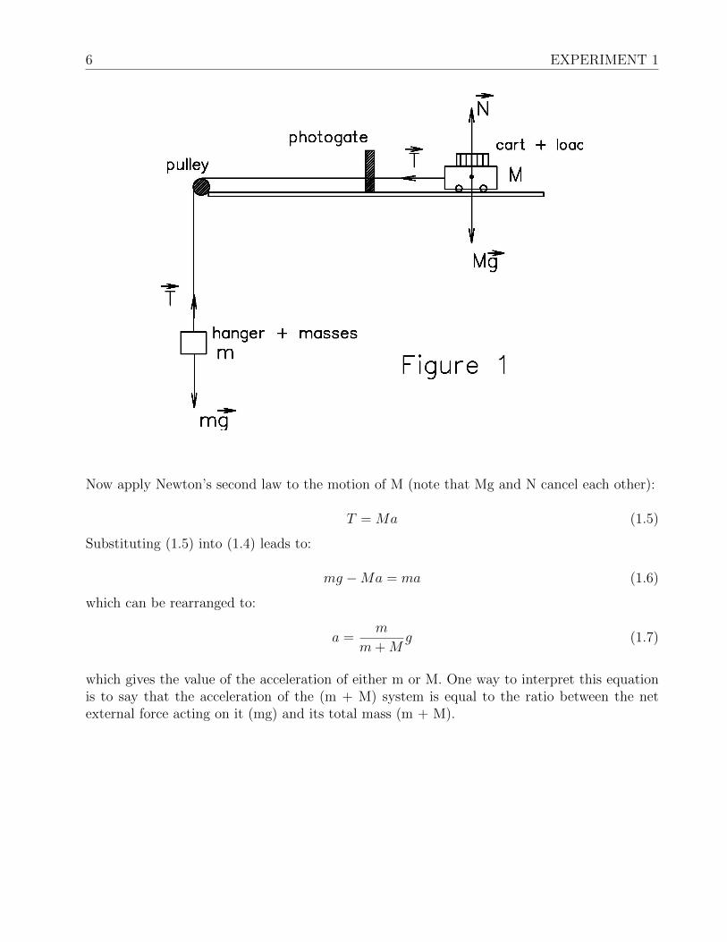
Consider the system shown in Figure 1. We shall neglect for now the rotational motion of thepulley, the frictional force acting on the system, and the mass of the string connecting the twomasses m and M . Let us apply Newton’s second law to the motion of m:

mg − T = ma (1.4)

6 EXPERIMENT 1

Now apply Newton’s second law to the motion of M (note that Mg and N cancel each other):

T = Ma (1.5)

Substituting (1.5) into (1.4) leads to:

mg −Ma = ma (1.6)

which can be rearranged to:

a =m

m+Mg (1.7)

which gives the value of the acceleration of either m or M. One way to interpret this equationis to say that the acceleration of the (m + M) system is equal to the ratio between the netexternal force acting on it (mg) and its total mass (m + M).

NEWTON’S SECOND LAW OF MOTION 7

Apparatus

• Computer

• Science Workshop Interface

• Dynamics Cart and Track System

• Mass Hanger and Mass Set (4x100g, 1x50g)

Procedure

1. At the start of your lab session, the Linear Dynamics System, Science Workshop interfacebox, and Dell computer will all be connected and ready to go. Familiarize yourself withthe system and the various components of the apparatus.

2. A linear motion timing experiment uses a photogate to measure the motion of an objectwith uniformly spaced flags. These are normally provided by the black stripes of a picketfence mounted on the object whose motion is being studied. Set up the apparatus asshown in Figure 1. Make sure the picket fence and track are free of dust and dirt. Ifneeded, ask for assistance from your laboratory instructor.

3. Follow the directions below to set up the DataStudio software:

• Double click on the Data Studio icon on the desktop.

• Choose No when the program asks whether DataStudio should choose an optionsset to load.

• Choose Create Experiment

The Experiment Setup window displaying the Science Workshop 750 Interface willappear.

8 EXPERIMENT 1

• Click on the first digital channel on the left.

• Choose Photogate & Picket Fence on the menu that appears.

• Deselect Acceleration, but make sure Position and Velocity are checked in theMeasurements tab.

• In the Constants tab, set the Band Spacing to 0.010m.

• Select Sampling Options at the top of the Experiment Setup window.

• In the Delayed Start tab, select Data Measurement and make sure that it says:

Position, Ch 1 (m)

Is Above 0 m.

• Click OK.

• You can now close the Experiment Setup window.

4. To set up how the data will be displayed, follow these steps:

• In the Displays column (at the left of the window) double click Graph.

• In the Choose a Data Source window, select Velocity, Ch1 (m/s).

• Maximize the graphical display.

5. Run 1: Place 150g (one 100 and one 50) on the cart and make sure there are no slottedmasses on the hanger. (The mass of the hanger, m, is 50g.) The mass of the cart (in-cluding the picket fence) is 510g. Therefore M = 0.510 kg + added masses. Record mand M in the data table.

6. Start data collection by clicking Start and immediately release the cart starting at oneend of the track. Make sure to halt the cart after it passes through the photogate. Stopdata collection by clicking Stop.

7. Look at the graph of Velocity vs Time on the screen. Use Scale to Fit to adjust theranges so the points take up most of the screen. If the line is uneven, delete the datafrom the run and repeat data collection until the plot is a relativity smooth line.

8. Once a smooth line is recorded, choose Linear Fit from the drop-down Fit menu toanalyze the velocity-vs-time plot. Compare the equation of the line (Y=mX+b) withequation (1.2) (velocity is on the y-axis, time is on the x-axis, etc.) and then extract andrecord the value of the acceleration aex and the initial velocity v0ex .

NEWTON’S SECOND LAW OF MOTION 9

9. Calculate and record the total mass, M +m, in the data table.

10. Using equation (1.1), calculate and record the force acting on the system, F = mg.

11. Then using Equation (1.7) calculate and record value of acceleration, ath = mm+M

g.

12. Consult section B.4 and then calculate and record the % difference between the theoreticaland experimental values for acceleration, |ath − aex|

|ath|· 100%.

13. RUN 2: Move 50 g from the cart load to the mass hanger. (M = 0.610kg and m =0.100kg.) Repeat steps 6 to 12.

14. RUN 3: Move an additional 50g from the cart load to the mass hanger. (M = 0.560kgand m = 0.150kg.) Repeat steps 6 to 12.

15. RUN 4: Add 150g to the cart load. (M = 0.710kg and m = 0.150kg.) Repeat steps 6 to12.

16. RUN 5: Add another 150g to the cart load. (M = 0.860 kg and m = 0.150 kg.) Repeatsteps 6to 12.

17. On one piece of graph paper, sketch each of the five lines generated in the above trialsand label each of them with the run # and corresponding equation. Be sure to title thegraph, and use regular increments on the axis and label them.

Discussion and Conclusion

Comment on whether your results agree with Newton’s Second Law. Explain. Outline anddiscuss at least two possible sources of error which may have occurred during the collection ofthe data and how they could have been avoided.

10 EXPERIMENT 1

Data Table: Newton’s Second Law

Run # 1 2 3 4 5

M(kg)m

(kg)aex

(m/s2)v0ex

(m/s)(m + M)

(kg)Fnet(N)ath

(m/s2)% difference

(%)

Date:

Instructor’s Name:

Instructor’s Signature:

Experiment 2

Atwood’s Machine

Introduction

Lab 2 continues with the study of Newton’s second law of motion. In this study an Atwood’smachine will be used which allows us to evaluate the situation where gravity is acting on bothmasses in the system rather than just one as in Lab 1.

Theory

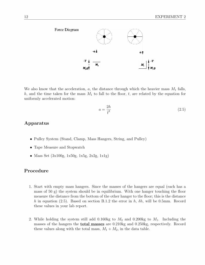
Atwood’s machine consists of two masses connected by a cord and suspended by a pulley asshown in the Force Diagram. Suppose for now that the pulley and cord have negligible massand that there is no friction acting on the system. In response to the downward force of gravity,the heavier mass M1 will fall, with an acceleration of magnitude a. If the cord is of fixed length,the lighter mass M2 must rise with an acceleration of magnitude a as well. Applying Newton’ssecond law to each mass gives:

M1g − T = M1a (2.1)

M2g − T = −M2a (2.2)

where we have chosen the positive direction to be downwards in each case. Notice also that themagnitude of the tension T is uniform throughout the cord.

We can solve for a by subtracting equation (2.2) from equation (2.1):

(M1 −M2)g = (M1 +M2)a (2.3)

If we include the effects of the frictional force, f , then equation (2.3) should be modified to:

(M1 −M2)g − f = (M1 +M2)a (2.4)

12 EXPERIMENT 2

We also know that the acceleration, a, the distance through which the heavier mass M1 falls,h, and the time taken for the mass M1 to fall to the floor, t, are related by the equation foruniformly accelerated motion:

a =2h

t2 (2.5)

Apparatus

• Pulley System (Stand, Clamp, Mass Hangers, String, and Pulley)

• Tape Measure and Stopwatch

• Mass Set (3x100g, 1x50g, 1x5g, 2x2g, 1x1g)

Procedure

1. Start with empty mass hangers. Since the masses of the hangers are equal (each has amass of 50 g) the system should be in equilibrium. With one hanger touching the floormeasure the distance from the bottom of the other hanger to the floor; this is the distanceh in equation (2.5). Based on section B.1.2 the error in h, δh, will be 0.5mm. Recordthese values in your lab report.

2. While holding the system still add 0.160kg to M2 and 0.200kg to M1. Including themasses of the hangers the total masses are 0.210kg and 0.250kg, respectively. Recordthese values along with the total mass, M1 +M2, in the data table.

ATWOOD’S MACHINE 13

3. Gently release the system from rest. With a stopwatch measure the time it takes M1 totravel the distance h from rest. Make three independent measurements of this time andrecord them as t1, t2 and t3 in the data table .

4. By consulting section B.1.3 and knowing that since you made three trials N=3, calculateand record the average time of fall, t = t1+t2+t3

3, the standard deviation of your time

measurements, σs.d. =√

(t1−t)2+(t2−t)2+(t3−t)23

, and the error in t, δt = σs.d.√3

.

5. Using equation (2.5), determine and record the acceleration, a = 2h

t2 , of the system.

6. Consult section B.3.4 to calculate the error in a, δa = a√

(1·δhh

)2 + (−2·δtt

)2 and record it.

7. Calculate the force acting on the system, F = (M1−M2)g, and assume the correspondingerror, δF , is zero since the error in the masses is negligible.

8. Repeat steps 3 through 7 five more times, each time moving 2g from M2 to M1 (thuskeeping the total mass of the system, M1 +M2, constant).

9. Use the data collected to plot a graph of Force versus Acceleration. Use the calculatedvalues of δa to draw horizontal error bars to scale. Determine the best line through yourpoints (It must intersect at least two points and have an equal number of points belowand above the line) and use the error bars to find the maximum (steepest) and minumum(shallowest) slopes.

10. Determine the value of the best slope, mbest, using two points you DID NOT plot, (x1, y1)and (x2, y2) and the formula: m = rise

run= y2−y1

x2−x1 . Similarly find the values of mmax andmmin.

11. Find the error in the slope, δm, by calculating mmax-mbest and mbest-mmin and choosingthe larger value .

12. Compare the equation of the line (Y=mX+b) with equation (2.4) (net force is on they-axis, acceleration is on the x-axis, etc.).

13. Based on the comparison in the previous step extract the value of the effective frictionalforce, f , acting on your system as well as it’s error, δf (see section B.3.1).

14 EXPERIMENT 2


Comment on whether your results agree with Newton’s Second Law. Explain. Outline anddiscuss at least two possible sources of error which may have occurred during the collection ofthe data and how they could have been avoided.

ATWOOD’S MACHINE 15

Data Table: Atwood’s Machine

M1

(kg)

M2

(kg)

(M1 +M2)(kg)

t1(s)

t2(s)

t3(s)

t(s)

σs.d.(s)

δt(s)

a(m/s2)

δa(m/s2)

F(N)

Date:



16 EXPERIMENT 2

Experiment 3

Measurement of the Acceleration ofGravity

Introduction

In this lab you will study free fall motion using the free fall adapter which plugs into photogatetimers and computer interfaces, allowing for a precise measurement of acceleration.

Theory

Free fall is the motion of any object subjected to the gravitational force exerted by the earth.The magnitude of this gravitational force is given by Newton’s formula:

F = GMEM

d2= G

MEM

(R + r)2(3.1)

where G is the gravitational constant, ME the mass of the earth, M the mass of the fallingobject, R the radius of the earth, and r the elevation of the object above the surface of theearth. If we defined the quantity g as:

g = GME

(R + r)2(3.2)

On the surface of the earth r is negligible in comparison to the much larger value of R; conse-quently, and to a high degree of accuracy, g can be considered constant.Combining equations (3.1) and (3.2) we get:

F = Mg (3.3)

Applying Newton’s second law of motion:

F = Ma (3.4)

18 EXPERIMENT 3

it becomes clear that the quantity g is nothing but the acceleration of a free fall motion, which,since it is independent of the mass of the falling object, is a constant regardless of how heavyor light the object is. We call g the acceleration of gravity.

As you already know, the equation of motion for a body starting from rest and undergoingconstant acceleration can be expressed as:

x =1

2at2 (3.5)

where x is the distance travelled, a the acceleration, and t the time elapsed. So the motion forfree fall with no initial velocity is simply given by:

d =1

2gt2 (3.6)

Apparatus

• Free Fall Adaptor (automatic ball release mechanism, receptor pad, controller box)

MEASUREMENT OF THE ACCELERATION OF GRAVITY 19

• Computer

• Science Workshop Interface

• Tape Measure

• 2 Steel Balls (13 and 16 mm)

Procedure

1. At the start of your lab session, the Free Fall Adaptor, Science Workshop interface box,and Dell computer will all be connected and ready to go.item Follow the directions below to set up the DataStudio software:

• Double click on the Data Studio icon on the desktop.

• Choose No when the program asks whether DataStudio should choose an optionsset to load.

• Choose Create Experiment

The Experiment Setup window displaying the Science Workshop 750 Interface willappear.

• Click on the first digital channel on the left.

• Choose Free Fall Adapter on the menu that appears.

• Deselect Acceleration, but make sure time is checked in the Measurements tab.

• Select Sampling Options at the top of the Experiment Setup window.

• In the Delayed Start tab, select time and set it to 0.

• Deselect the start signal generation before start condition option.

• In the Automatic Stop tab, select data measurement but don’t change theoptions.

• Click OK.

• You can now close the Experiment Setup window.

2. To set up the timing window, look in the Displays column (at the left of the window)and double click 3.14 DIGITS.

3. The Free Fall Adapter consists of an automatic ball release mechanism, a receptor pad,and a controller box (see Figure 1). The controller box plugs into a computer interfacewhich is basically a digital clock started when the ball is released and stopped when the

20 EXPERIMENT 3

ball hits the pad. The digital reading of the timer is then simply the time taken by theball to fall a distance d (see Figure 2). Set up the apparatus as shown in Figure 2. Ifneeded, ask for assistance from your laboratory instructor.

4. Mount the 16mm diameter steel ball tightly in the Ball Release Mechanism and beingas accurate as possible (so that δd can be assumed to be zero) set the distance from thebottom of the ball to the top of the pad d to 1.00m and record it in Data Table 1. Makeseveral trials to be sure the ball will hit the center of the Receptor Pad when released.

5. Take a first measurement of t and record it in the table as t1. Repeat the measurementtwice more and record these values as t2 and t3.

6. By consulting section B.1.3 and knowing that since you made three trials N=3, calculateand record the average time of fall, t = t1+t2+t3



(t1−t)2+(t2−t)2+(t3−t)23


.

7. Square the value of t and consult section B.3.4 to find the corresponding error, δt2

= t2·2·δtt

.Remember to record all values in the tables.

8. Repeat steps 4 through 7 for the 13 mm steel ball and record the values in Data Table 2.

9. Repeat steps 4 through 8 for the following values of d: 1.05, 1.10, 1.15, 1.20, 1.25, 1.30,and 1.35. Record all your measurements in the Data Tables.

10. Plot a graph of Distance versus Time2, for the 16mm ball bearing. Use the calculatedvalues of δt

2to draw horizontal error bars to scale. Determine the best line through your

points (It must intersect at least two points and have an equal number of points belowand above the line) and use the error bars to find the maximum (steepest) and minumum(shallowest) slopes.


run= y2−y1




13. Compare the equation of the line (Y=mX+b) with equation (3.6) (distance is on they-axis, time squared is on the x-axis, etc.).

14. Based on the comparison in the previous step extract the value of the gravitational ac-celeration, g16, acting on your system as well as it’s error, δg16 (see section B.3.1).

15. Repeat steps 10 through 14 for the 13 mm steel ball


Comment on whether your results support that the acceleration of gravity is independent ofmass. Explain. Outline and discuss at least two possible sources of error which may haveoccurred during the collection of the data and how they could have been avoided.

22 EXPERIMENT 3

Data Table 1: Free Fall of a 16mm Steel Ball

d(m)

t1(s)

t2(s)

t3(s)

t(s)

σsd(s)

δt(s)

t2

(s2)

δt2

(s2)

Date:




Data Table 2: Free Fall of a 13mm Steel Ball

d(m)

t1(s)

t2(s)

t3(s)

t(s)

σsd(s)

δt(s)

t2

(s2)

δt2

(s2)

Date:



24 EXPERIMENT 3

Experiment 4

Kinematics: Constant Acceleration

Introduction

In this experiment a ‘dynamics cart’ will be launched across the floor, and its change in velocity

(acceleration) measured. The results will then be analyzed using two different methods of error

analysis. Theory

If the acceleration of the cart does remain constant throughout its journey, the calculated valuesof tth, the time required to travel the distance d, should be equal to the directly measured value,tex. To calculate tth the distance equation is used,

d = votth +1

2at2th (4.1)

Now if both the acceleration a and the initial velocity vo are known, then the time requiredto travel an intermediate distance tth can be calculated. We do this by applying the quadraticformula,

if ax2 + bx+ c = 0 then x = −b±√b2−4ac

2a, to the distance equation (4.1).

The dynamics cart will be launched across the floor using the built in spring plunger. The cartwill then accelerate (in everyday language we often use the word ‘decelerate’ for an object thatslows down. In Physics we normally use the word ‘accelerate’ for objects that speed up or slowdown as they are just two aspects of the same effect) due to various effects of friction (frictionin the wheel bearings, ‘rolling’ friction) and the slope of the floor.

26 EXPERIMENT 4

Eventually the cart will roll to a stop. The total distance covered is denoted D and the totalelapsed time from the launch to the stop is denoted T .

Then the average velocity of the cart on its journey is given by:

vav =D

T(4.2)

If the acceleration of the cart remains constant throughout its journey across the floor, thenthe initial instantaneous velocity of the cart at the moment it is launched is given by:

vo = 2vav =2D

T(4.3)

The value of this constant acceleration is then given by:

a =change in v

change in t=vfinal − vinitialtfinal − tinitial

=0− voT − 0

= −voT

= −2D

T 2(4.4)

Note: the acceleration is negative, ie. the cart is slowing down.

Apparatus

• Dynamics Cart (PASCO ME-9430)

• Stopwatch with lap timer

• Tape Measure and Electrical Tape

KINEMATICS: CONSTANT ACCELERATION 27

Procedure

1. Mark a fixed launch point for the cart. To launch the cart with reasonable repeatability,you need to cock the spring plunger. To cock the plunger, push the plunger in, and thenpush the plunger upward slightly to allow one of the notches in the plunger bar to catchon the edge of the small metal bar at the top of the hole.

2. Launch the cart a couple of times to roughly determine its range. Now mark a distance dthat is a bit more than halfway between the start and finish. Measure the distance fromthe launch point to d and record it above the data table in your lab report (Data Table 1).

3. Using the stopwatch (make sure it is in ‘cumulative mode’) and the meter stick, it ispossible to measure t, T and D for each launch. You will probably want to practice thisa few times before you start recording data. The stopwatch is started when the cart islaunched, the t is recorded using the ‘lap time’ feature, and the total time for the journeyis recorded by stopping the stopwatch. The total distance the cart travels, D, is deter-mined using the tape measure.

Note: To reduce errors due to reaction times it is important that the person who launchesthe cart also do the timing. You should take turns. Also, trials in which the launcher/timerthinks that there was some distraction or other unusual error that interfered with the mea-surement should not be recorded, as this will decrease the accuracy of data.

4. Launch the cart and record t, T and D for six trials in a table similar to the one shownData Table 1.

Note: We will be switching back and forth between absolute and relative (%) errors tosimplify the error calculation (yes, this is the easy way). This allows us to simply add theerrors in quadrature, which is done by combining the errors using the following formula:

Error =√

(Error1)2 + (Error2)2

• For addition/subtraction add the absolute errors in quadrature.

• For multiplication/division add the relative (%) errors in quadrature.

• For powers multiply the relative (%) errors by the exponent.

• For coefficients the relative (%) errors are unaffected.

28 EXPERIMENT 4

Although some of the following looks intimidating, if you follow the steps givenin the manual carefully by substituting in your values, it is time consumingbut not difficult.

5. Calculate the relative errors of d, D, T and tex and fill them into your table. A reason-able error estimate for hand timed intervals (due to human reaction time) is ±0.09 s anddistances should be measured to within ±0.0005 m. Show your calculations as in thefollowing example:

Sample calculation of relative errors:

In a case where,

d = (1.1000± 0.0005)m

D = (1.8000± 0.0005)m

T = (7.84± 0.09)s

tex = (3.12± 0.09)s

the absolute errors are converted to relative (%) errors by:

relative error =absolute error

value of variable∗ 100 %

For example:

d = 1.1000m± (0.0005m

1.1000m∗ 100%) = 1.1000m± 0.05%

D = 1.8000m± (0.0005m

1.8000m∗ 100%) = 1.8000m± 0.03%

T = 7.84s± (0.09s

7.84s∗ 100%) = 7.84s± 1.14%

tex = 3.12s± (0.09s

3.12s∗ 100%) = 3.12s± 2.88%


6. Work out vo, a and their absolute errors. Show your calculations in the following way:

Sample calculation of vo:

vo =2D

T=

2(1.8000m± 0.03%)

(7.84s± 1.14%)

since this is division the relative errors must be added in quadrature:

vo = 0.459m/s±√

(0.03%)2 + (1.14%)2 = 0.459m/s± 1.14%

The relative (%) errors are converted to absolute errors by:

absolute error =relative error

100 %∗ value of variable

For example:

vo = 0.459m/s± (1.14%

100%∗ 0.459m/s) = (0.459± 0.005)m/s

Sample calculation of a:

a = −2D

T 2= −2(1.8000m± 0.03%)

(7.84s± 1.14%)2= −3.6000m± 0.03%

61.5s2 ± 2.28%

Note: When adding in quadrature the relative error of T is multiplied by 2 because T issquared in the equation for a.

a = −0.0585m/s2 ±√

(0.03%)2 + (2.28%)2 = −0.0585m/s2 ±%

a = −0.0585m/s2 ± (2.28%

100%∗ .0585m/s2) = (−0.059± 0.001)m/s2

30 EXPERIMENT 4

7. For trial 1 only, calculate the expected (theoretical) value for t. Follow the sample calcu-lation exactly and show all the steps in your lab.

Sample calculation of tth:

In an equation of the form:

1/2at2th + votth − d = 0

the quadratic equation can be used to solve for tth:

tth =−vo ±

√v2o − 4(1

2a)(−d)

2(12a)

which can be simplified to give:

tth =−vo ±

√v2o + 2ad

a

(a) plug in the values:

tth =−(0.459m/s± 1.14%)±

√(0.459m/s± 1.14%)2 + 2(−0.059m/s2 ± 2.28%)(1.100m± 0.05%)

(−0.059m/s2 ± 2.28%)

(b) do the exponent and multiplication:

tth =−(0.459m/s± 1.14%)±

√(0.211m2/s2 ± 2.28%)− (0.130m2/s2 ± 2.28%)

(−0.059m/s2 ± 2.28%)

(c) convert the errors inside the square root to absolute errors:

tth =−(0.459m/s± 1.14%)±

√(0.211m2/s2 ± 0.005m2/s2)− (0.130m2/s2 ± 0.003m2/s2)

(−0.059m/s2 ± 2.28%)

(d) do the subtraction inside the square root:

tth =−(0.459m/s± 1.14%)±

√0.081m2/s2 ± 0.006m2/s2

(−0.059m/s2 ± 2.28%)


(e) convert the errors back to relative errors:

tth =−(0.459m/s± 1.14%)±

√0.081m2/s2 ± 7.4%

(−0.059m/s2 ± 2.28%)

(f) do the square root:

tth =−(0.459m/s± 1.14%)± (0.285m/s± 3.7%)

(−0.059m/s2 ± 2.28%)

(g) convert the errors in the numerator to absolute errors:

tth =−(0.459m/s± 0.005m/s)± (0.28m/s± 0.01m/s)

(−0.059m/s2 ± 2.28%)

(h) do the addition/subtraction (note: you will have two possible values):

tth =−(0.18m/s± 0.01m/s)

(−0.059m/s2 ± 2.28%)OR tth =

−(0.74m/s± 0.01m/s)

(−0.059m/s2 ± 2.28%)

(i) convert the error in the numerator back to relative error:

tth =−(0.18m/s± 5.56%)

(−0.059m/s2 ± 2.28%)OR tth =

−(0.74m/s± 1.35%)

(−0.059m/s2 ± 2.28%)

(j) do the division:

tth = 3.05s± 6.01% OR tth = 12.5s± 2.65%

Whew! We’re finished! Clearly the first t value is the one to choose since the secondone is a time after the cart has stopped. Note that the resultant error is rather large(±6.01% or ± .2s). This is because of the subtraction that yielded a relatively smallresult although the error grew in each step.

8. Find the difference (and corresponding error) between the theoretical and measured tvalues. Call these values x and δx respectively. In this sample our measured value istex = (3.1± 0.2)s so the difference is:

x = tex − tth = (3.12± 0.09)s− (3.1s± 0.2)s = (0.02± 0.2)s

In this case, although there is a difference between the two t values, our error analysisshows that this difference is small compared to the error. For this trial, the hypothesisthat the acceleration is constant is supported.

32 EXPERIMENT 4

9. Now calculate and record the values of vo, a, tth and x for the rest of the trials.

10. Compute the average time difference from your six trials. Also calculate the standarddeviation of the time difference from your set of six trials.

Sample calculation of x and σx:

If the x values are: (0.2 ± 0.4)s, (0.8 ± 0.3)s, (−0.3 ± 0.4)s, (0.1 ± 0.4)s, (0.7 ± 0.3)s,(−0.6± 0.3)s. Consider these values as x1, x2, x3, x4, x5 and x6 respectively.

Calculate the mean value of x. We will call it x.

x =1

N

N∑i=1

xi =1

6(0.2s+ 0.8s+ (−0.3s) + 0.1s+ 0.7s+ (−0.6s)) = 0.15s

where N is the number of trials.

Estimate the standard deviation, σx, in the set of trial values. In this calculation we don’tuse the calculated error values, instead we look at how much each xi value varies from xand combine this information to give us σx. This is done using the following equation:

σx =

√√√√ 1

N

N∑i=1

(xi − x)2

Plug in the values and solve:

σx =

√1

6[(0.2− 0.15)2 + (0.8− 0.15)2 + (−0.3− 0.15)2 + (0.1− 0.15)2 + (0.7− 0.15)2 + (−0.6− 0.15)2]

=

√1

6(1.5s2) =

√0.25s2 = 0.50s

So the value determined from our multiple trials is tex−tth = (0.15±0.50)s. From this weconclude that although the mean value is not zero, it differs from zero less than the stan-dard deviation. Which means that zero is in the defined range (ie. 0.15s−0.50s = −0.35s,crosses zero). This supports the hypothesis that the acceleration of the cart remains con-stant. Note also that the standard deviation is roughly the same size as the errors in theindividual trials.



Comment on whether your results support the hypothesis of constant acceleration. Explain.Outline and discuss at least two possible sources of error which may have occurred during thecollection of the data and how they could have been avoided.

34 EXPERIMENT 4

Data Table: Kinematics

tex(s)

δtex(%)

T

(s)

δT(%)

D(m)

δD

(%)

vo(m/s)

δvo n/a n/a n/a n/a n/a(m/s)

a

(m/s2)

δa n/a n/a n/a n/a n/a(m/s2)

tth(s)

δtth n/a n/a n/a n/a n/a(s)

x(s)

δx n/a n/a n/a n/a n/a(s)

Date:



Experiment 5

Hooke’s Law and Simple HarmonicMotion

Introduction

Hooke’s law describes the motion of a spring. This law is exactly valid only in the case of anideal (i.e., perfectly elastic) spring. However, we can do experiments with real springs whichexhibit ideal behavior over a limited range of extension. We will also study one of the mostinteresting types of motion in nature, the so-called simple harmonic motion. Such a motiontakes place whenever the force acting on a system takes the form of a restoring force of theform given below. Examples include the oscillatory motion of a mass-spring system and theperiodic motion of a pendulum.

Theory

Consider the mass-spring system in the following Force Diagram. The spring elastic force actingon the mass is a restoring force having the form:

F = −kx (5.1)

where x = (xf − x0) is the amount of stretching undergone by the spring away from its un-stretched position x0. k is a constant characteristic of the spring called the force constant. Theminus sign indicates that the tendency of the spring force is to oppose this stretching and pushthe system back toward the unstretched position (hence the term restoring force). Equation(5.1) is called Hooke’s law, which we will apply to two cases.

Static case: When the system is in equilibrium, equation (5.1) is simply a statement that theamount of extension x is proportional to the force applied to the spring which in our case isequal in magnitude to the weight of the suspended mass:

36 EXPERIMENT 5

|F | = Mg = k(xf − x0) = kx (5.2)

Note: We have neglected the small mass of the spring compared to the suspended mass.

Dynamic case: If the mass is pulled down from its equilibrium position by a small distanceand released gently, then what follows is an oscillatory, periodic motion (or simple harmonicmotion) wherein the block moves up and down around the equilibrium position. Such a motionis characterized by its period of oscillation T which is given by:

T = 2π

√M

k(5.3)

Apparatus

• Hooke’s Law Apparatus (Stand, Ruler, Mass Hanger)

• Stopwatch

• 2 Springs (small and large)

• Mass Set (1x100g, 5x20g, 1x10g)

HOOKE’S LAW AND SIMPLE HARMONIC MOTION 37

Procedure

Static Case:

1. Using the larger spring and with no mass on the hanger, measure the position of thepointer attached to the spring, x0. Based on section B.1.2 the error in x0, δx0, will be 0.5mm. Record these measurements the appropriate data table.

2. Add 10g to the mass holder whose mass is 10 g. Record the total mass acting on thespring, M = 0.020kg, in the appropriate data table. Calculate and record the force beingexerted on the spring due to gravity, F = Mg. Assume the corresponding error, δF , iszero since the error in the masses is negligible.

3. Measure the pointer’s new positon, xf . Since the measuring device being used is the sameas that used to measure x0, the error in xf , δxf , will be the same as δx0, 0.5mm.

4. Calculate and record the total displacement, x = (xf − x0). By consulting section B.3.2,

find the error in displacement, δx =√

(δx0)2 + (δxf )2.

5. Repeat steps 2 through 4 nine times, each time adding 10 g to the hanger and recordyour results in the appropriate data table.

6. Use the data collected to plot a graph of Force versus Displacement and test for linearity.Determine the best line through your points (It must intersect at least two points andhave an equal number of points below and above the line)


run= y2−y1

x2−x1 .

8. Compare the equation of the line (Y=mX+b) with equation (5.2) (force is on the y-axis,displacement is on the x-axis, etc.).

9. Based on the comparison in the previous step deduce the value of the spring constant andcall it kLarge.

10. Repeat steps 1 through 9 for the smaller spring and call the spring constant you deducein this case, kSmall.

38 EXPERIMENT 5

Dynamic Case:

11. Now you are to measure the period of oscillation of the simple harmonic motion of themass-spring system and compare it to equation (5.3). First measure and record the massof the larger spring, Mspring.

12. You will begin by adding 100g to the 10g hanger. Record the total mass, M = 0.110kg inData Table 2. Assume the corresponding error, δM , is zero since the error in the massesis negligible.

13. Gently set the system in motion by slightly lifting the mass and then releasing it. Tryyour best to obtain up-and-down oscillations with no twisting or swaying of the spring(this would complicate the motion and affect the measured values). Also, make sure thatthe oscillations occur inside the region where Hooke’s law is applies (otherwise equation(5.3) would cease to be valid). Wait a few moments to ensure the stability of the oscil-lation then measure the time t for 10 complete oscillations (cycles). Assume an error int of δt = 0.09 s. (0.09 s should be a reasonable error reflecting how accurately and howfast you are timing the start and end of the 10 cycles.)

14. Deduce the value of the period, T = t10

. Consult section B.3.1 to calculate the error inT , δT = δt

10. Continue to record your data and results in Data Table 2.

15. Calculate and record T 2. By consulting section B.3.4 you can find its corresponding error,δT 2 = T 2 · 2·δT

T.

16. Repeat steps 11 through 15 five times, each time adding 20g and record your results inData Table 2.

17. Equation (5.3) can be rearranged algebraically to give:

M =k

4π2T 2 (5.4)

Use the data collected to plot a graph of Mass vs. Period2 and test for linearity. Use thecalculated values of δT 2 to draw horizontal error bars to scale. Determine the best linethrough your points (It must intersect at least two points and have an equal number ofpoints below and above the line) and use the error bars to find the maximum (steepest)and minumum (shallowest) slopes.



run= y2−y1



20. Compare the equation of the line (Y=mX+b) with equation (5.4) (mass is on the y-axis,period squared is on the x-axis, etc.).

21. Based on the comparison in the previous step extract the value of the spring constant,k = 4π2 ·m. Also consult section B.3.1 to find its error, δk = 4π2 · δm.

22. In addition find and record the value of the best y-intercept, b, the maximum y-intercept,bmax, and the minimum y-intercept, bmin. Find δb by calculating bmax-bbest and bbest-bminand choosing the larger value .

23. If the spring mass, Mspring, is included, it can be shown that equation (5.4) should bereplaced by the more accurate expression:

M +Ms =k

4π2T 2 (5.5)

Which can be rearranged to give:

M =k

4π2T 2 −Ms (5.6)

Compare this equation (5.6) to the straight line equation and determine the experimentalvalue of the mass of the spring, Mspringex = −b, and its error, δMspringex = δb.


Comment on whether your results agree with Hooke’s Law. Explain. Outline and discuss atleast two possible sources of error which may have occurred during the collection of the dataand how they could have been avoided.

40 EXPERIMENT 5

Data Table 1: Hooke’s Law for the Larger Spring

xo ± δxo =

M F xf ± δxf x± δx(kg) (N) (m) (m)

Date:




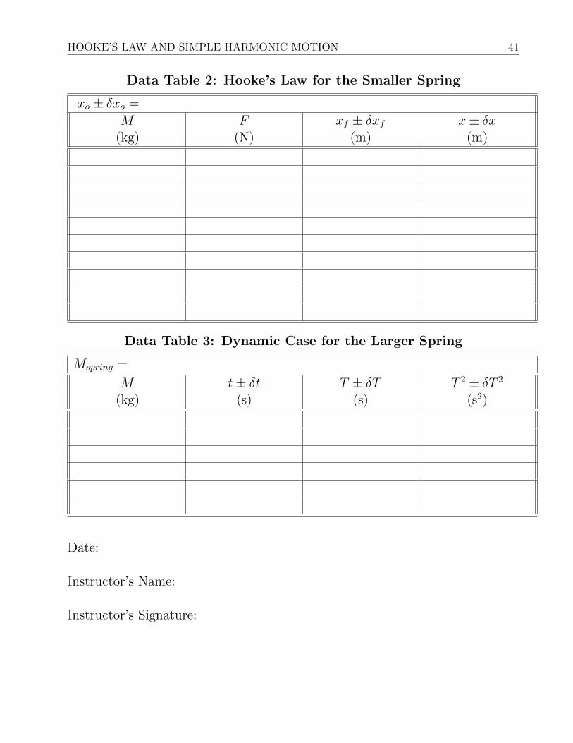
Data Table 2: Hooke’s Law for the Smaller Spring

xo ± δxo =

M F xf ± δxf x± δx(kg) (N) (m) (m)

Data Table 3: Dynamic Case for the Larger Spring

Mspring =

M t± δt T ± δT T 2 ± δT 2

(kg) (s) (s) (s2)

Date:



42 EXPERIMENT 5

Experiment 6

The Simple Pendulum

Introduction

Lab 5 looked at simple harmonic motion of a mass-spring system whereas in Lab 6 you willstudy the periodic, simple harmonic motion of a pendulum. We will use the method of dimen-sional analysis to construct a relationship between the period T of the pendulum and the lengthl of the string and experimentally test the constructed relationship using graphical analysis.

Theory

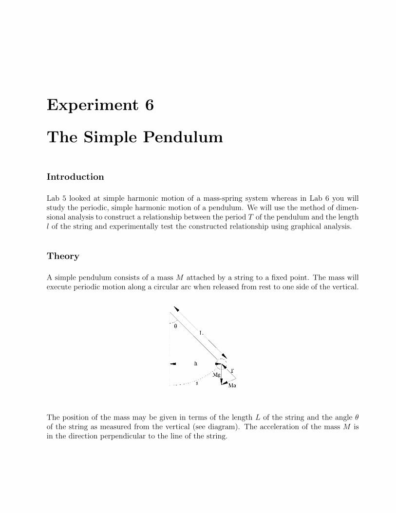
A simple pendulum consists of a mass M attached by a string to a fixed point. The mass willexecute periodic motion along a circular arc when released from rest to one side of the vertical.

The position of the mass may be given in terms of the length L of the string and the angle θof the string as measured from the vertical (see diagram). The acceleration of the mass M isin the direction perpendicular to the line of the string.

44 EXPERIMENT 6

Using Newton’s second law gives:

F = Mg sin θ = Ma (6.1)

for the magnitude of the acceleration a.

Notice that we have taken the component of the weight along the direction perpendicular to theline of the string. For large angles, further analysis of the motion of the mass using equation(6.1) is complicated. However, if we restrict our investigation to small angles, we may makeapproximations which simplify matters. For small angles we have:

sin θ = h/L ≈ s/L (6.2)

where θ is in radians.

Putting equation (6.2) into equation (6.1) gives us an expression for the magnitude of a:

a ≈ (g/L)s (6.3)

Notice that the acceleration is in the direction back towards the vertical. Whenever the accel-eration is proportional and opposite to the displacement, the motion is called simple harmonicmotion. This type of motion occurs for the simple pendulum when the displacement, s, is small.

We can construct a relationship between the period T and the length L of the pendulum byusing the method of dimensional analysis. In this method we ensure that the dimensions (units)are the same on both sides of the equation. We expect the period to depend on the accelerationdue to gravity, g, because we know that no oscillations would occur if g was zero. We thereforeexpect a relationship of the form:

T = cLαgβ, (6.4)

where c is a numerical constant having no dimensions, and the exponents α and β are to befound using dimensional analysis.

It can be shown that, in order that equation (6.4) provide a good estimate for the period T ofthe simple pendulum, the magnitude of s/L should typically be no bigger than about 0.1.

Apparatus

• Pendulum System (Stand, string and bob)

• Meter stick and Stopwatch

THE SIMPLE PENDULUM 45

Advance Preparation: It is essential that you read the Appendix on DimensionalAnalysis and do steps 1. and 2. in the data section of your lab report before coming to thelab.

1. Using the method of dimensional analysis (see the Appendix), determine the values ofthe exponents α and β in equation (6.4). Record your equation (6.4) with these values ofα and β.

2. Explain how you can test your equation using graphical analysis. What should be plottedon the “y–axis”? What should be plotted on the “x–axis”? Write your expression in thestandard form y = mx+ b. What is your expression for the slope m?

Procedure

3. Spend a few moments familiarizing yourself with the apparatus and the method of ad-justing the length of the string.

4. Start by adjusting the string to have a length of 20cm from the fixed point to the bottomof the mass and record this length, L, in the data table. Also record the error in thelength, δL, which based on section B.1.2 will be 0.5mm.

5. Pull the mass to one side of the vertical. Make sure that the ratio s/L (see Diagram) is nobigger than 0.1. Release the mass from rest and start the stopwatch at the same instant.Allow the bob to oscillate through 10 cycles and stop the stopwatch at the instant thatthe mass reaches its greatest deflection from the vertical. Record your value for the totaltime, t1, of the 10 cycles.

6. Repeat step 5 four times with the same length of string. Record the times for 10 cyclesas t2, t3, t4, and t5.

7. By consulting section B.1.3 and knowing that since you made five trials N=5, calculateand record the average time of fall, t = t1+t2+t3+t4+t5



(t1−t)2+(t2−t)2+(t3−t)2+(t4−t)2+(t5−t)25


.

8. By dividing t by the number of oscillations in each trial it is possible to find the averageperiod, T = t

10. Consult section B.3.1 to calculate the error in T , δT = δt

10.

46 EXPERIMENT 6

9. Repeat steps 4 through 8 for lengths of 25, 30, 35, 40, 45, and 50 cm. Record all yourvalues in the data table.

10. Calculate and tabulate your values for what you determined y, δy, x and δx to be in step 2.

11. Plot a graph of y versus x. Use the calculated values of δx and δy to draw horizontaland vertical error bars respectively. Determine the best line through your points (It mustintersect at least two points and have an equal number of points below and above theline) and use the error bars to find the maximum (steepest) and minimum (shallowest)slopes.


run= y2−y1



14. Using the expression for slope you found in step 2 and your values for the slope andits error, determine the numerical value of c and its error. Find the percent differencebetween this value and the expected value of 2π.

15. Examine your graph, if you have been careful enough in collecting your data, you maywell find that x−intercept 6= 0. After thinking about it, you will agree that the distanceto the center of the mass is the correct length to use in equation (6.4). Therefore youshould indeed expect that the x− intercept will be nonzero. So equation (6.4) should bemodified to read:

T = c(L− r)αgβ, (6.5)

where L is the length of the string and r is the radius of the weight. Measure and recordthe radius of the weight r, at the end of the string.

16. Find and record the value of the best x − intercept, Xintercept, the maximum x −intercept, Xmax, and the minimum x− intercept, Xmin. Find δXintercept by calculatingXmax-Xbest and Xbest-Xmin and choosing the larger value . Find the percent differencebetween the radius of the ball and the x-intercept.

THE SIMPLE PENDULUM 47


Comment on whether your results support the constructed relationship between period andlength. Explain. Outline and discuss at least two possible sources of error which may haveoccurred during the collection of the data and how they could have been avoided.

48 EXPERIMENT 6

Data Table: Simple Pendulum

L(m)

δL

(m)

t1(s)

t2(s)

t3(s)(s)

t4(s)(s)

t5(s)(s)

t

(s)

σs.d.(s)

δt(s)

T

(s)

δT(s)

Date:



Experiment 7

Rotation and Moment of Inertia

Introduction

This experiment examines rotational motion and the moment of inertia. We will experimentallytest the theoretical relationship between the torque applied to a wheel, the acceleration of thewheel, and the moment of inertia of the wheel using the method of graphical analysis.

Theory

Consider a wheel and an axle attached by radial spokes. A thin cord is wound around the wheeland the hanging end is used to suspend a mass, M , as shown in the diagram. To investigatethe motion of the system, we need to specify the forces acting on the mass and the torquesacting on the wheel.

The mass experiences a downward force, Mg, due to gravity, and an upward force, T , fromthe tension in the cord. The mass will accelerate downward with magnitude a according toNewton’s second law:

Mg − T = Ma (7.1)

Notice that the tension, T , must be less than the force, Mg, if the mass is to accelerate down-ward.

Given that the mass accelerates downward, the wheel will rotate with angular acceleration, α.The tension in the cord acts downward at the edge of the wheel and thus produces a torque ofmagnitude, τ = RT , on the wheel, where R is the radius of the wheel.

Assuming that the torque due to friction, τf , also has constant magnitude, the magnitude ofthe angular acceleration, α, is given by

50 EXPERIMENT 7

RT − τf = Iα (7.2)

where I is the moment of inertia of the wheel.

The angular and linear accelerations are related by

a = Rα (7.3)

because the acceleration of the hanging mass and the acceleration of the edge of the wheel havethe same magnitude.

Substituting equation (7.3) into equation (7.2) we get:

RT − τf =Ia

R(7.4)

To clearly show how tension, T , and acceleration, a, are related, we rearrange equation (7.4):

T =I

R2a+

τfR

(7.5)

ROTATION AND MOMENT OF INERTIA 51

The tension, T , can be obtained from equation (7.1) but first we need to find the acceleration,a. We know the acceleration of the mass at the end of the cord is given in terms of the distance,h, through which it falls in a time, t, by:

a =2h

t2 (7.6)

Then we rearrange equation (7.1) to calculate T :

T = M(g − a) (7.7)

Apparatus

• Rotodyne Wheel and Wheel Mounting Masses (4x225g)

• Stand and Clamp

• String and Stopwatch

• Mass Hanger (6g) and Mass Set (2x20g, 1x10g, 1x5g)

Procedure

Determining the Moment of Inertia of the Wheel:

1. Spend a few moments familiarizing yourself with the apparatus and thinking about thebest way to collect the data. Note that the radius of the wheel is R = 0.20m.

2. Start by selecting the position from which you will release the hanging mass. Measureand record the height h through which the hanging mass will descend after it is released.Also record the error in the height, δh, which based on section B.1.2 will be 0.5mm.

3. For your first trial, let the hanging mass, M , consist of the hanger (5g), with a 5g slottedmass added, for a total of 11g. Record this value in Data Table 1.

4. Release the mass from rest and start the stopwatch at the same instant. Wait for themass to reach the floor and stop the stopwatch at the instant that the mass comes intocontact with the floor. Record your value for the total time, t1 in Data Table 1.

52 EXPERIMENT 7

5. Repeat four more trials for the same mass. Record the times of descent as t2, t3, t4, and t5.

6. By consulting section B.1.3 and knowing that since you made five trials N=5, calculateand record the average time of fall, t = t1+t2+t3+t4+t5



(t1−t)2+(t2−t)2+(t3−t)2+(t4−t)2+(t5−t)25


.

7. Use equation (7.6) to calculate the acceleration: a = 2h

t2 . Consult section B.3.4 to calcu-

late the error in a, δa = a√

(1·δhh

)2 + (−2·δtt

)2.

8. Also use equation (7.7) to calculate the tension: T = M(g− a). Consult section B.3.2 to

calculate the error: δT =√

(Mδg)2 + (Mδa)2. Assume that the error in acceleration dueto gravity is zero.

9. Repeat steps 4 through 8 for masses of 20, 30, 40, 50 and 60 g (These values include the5g of the hanger.) Record your values in Data Table 1.

10. Use the data collected to plot a graph of Tension versus Acceleration. Use the calculatedvalues of δa and δT to draw horizontal and vertical error bars respectively. Determinethe best line through your points (It must intersect at least two points and have an equalnumber of points below and above the line) and use the error bars to find the maximum(steepest) and minumum (shallowest) slopes.


run= y2−y1



13. In addition find and record the value of the best y-intercept, b, the maximum y-intercept,bmax, and the minimum y-intercept, bmin. Find δb by calculating bmax-bbest and bbest-bminand choosing the larger value .

14. Compare the equation of the line (Y=mX+b) with equation (7.5) (tension is on the y-axis, acceleration is on the x-axis, etc.).


15. Based on the comparison in the previous step obtain the values of the experimental mo-ment of inertia, I0 = R2 ·m and the frictional torque, τf = R · b. Consult section B.3.1to find their errors, δI0 and δτf .

Changing the Moment of Inertia of the Wheel:

16. Adding mass to the wheel should change its moment of inertia. Attach two additionalmasses to the wheel by screwing them into the 4th hole from the axle (each added mass is225g); select holes which are diametrically opposite from the axle.

17. Calculate the new theoretical value of inertia using:

Itheory = I0 +Mwr2 (7.8)

where I0 is the value you found in step 15, Mw is the total mass added to the wheel, and ris the distance from the axle to the points at which the masses were added (r = 0.15 m).See section B.3.2 for how to calculate δItheory.

18. Now repeat steps 4 through 8 excluding error analysis with a hanging mass, M=60g.Record your values in Data Table 2. Rearrange either equation (7.4) or (7.5) and use itto calculate an experimental value for Iexp.

19. Repeat steps 17 through 18 with 4 masses screwed into the 4th holes from the axle.


Comment on whether your experimental results agree with the theoretical predictions. Explain.Outline and discuss at least two possible sources of error which may have occurred during thecollection of the data and how they could have been avoided.

54 EXPERIMENT 7

Data Table 1: Determining the Original Moment of Inertia

M(kg)

t1(s)

t2(s)

t3(s)

t4(s)

t5(s)

t

(s)

σs.d.(s)

δt(s)

a(m/s2)

δa

(m/s2)

T(N)

δT

(N)

Date:




Data Table 2: Changing the Moment of Inertia

Mw

(kg)

M(kg)

t1(s)

t2(s)

t3(s)

t4(s)

t5(s)

t

(s)

a

(m/s2)

T(N)

Iexp(kg m2)

Itheory(kg m2)

δItheory(kg m2)

Date:



56 EXPERIMENT 7

Experiment 8

Standing Waves on a String

Introduction

This experiment will be your first introduction to waves. You will generate standing waves in ataut string and use the method of dimensional analysis to construct a theoretical relationshipbetween the wavelength λ of the standing waves and the tension T in the string.

Theory

Standing waves can be generated on a string by holding one end fixed and moving the otherend up and down with simple harmonic motion of frequency f . A “transverse” wave travelsdown the string, is reflected at the fixed end, then travels back toward its starting point. Wecan think of the overall wave motion of the string as being due to the combination of twowavetrains having the same frequency but traveling in opposite directions. If the string has“just the right length”, the result will be a standing wave as shown in the diagram. A standingwave has a stable pattern with oscillating loops of length λ/2. The stationary points betweenthe loops are called nodes, and the points midway between the nodes, where the amplitudes ofoscillation are greatest, are called antinodes.

We can construct a relationship between the wavelength λ, frequency f , and tension T by usingthe method of dimensional analysis. In this method we relate physical quantities using empir-ical knowledge or intuitive insight, and we ensure that the dimensions (units) are the same onboth sides of the equation. For example, we know from our experience with musical instrumentsthat a heavier string vibrates at a different frequency than a lighter string. We therefore expectour relationship to involve the mass per unit length, ρ. (Note, this is LINEAR density.)

58 EXPERIMENT 8

It is reasonable to try the following expression as a relationship between λ, ρ, f , and T :

λ = cραfβT γ (8.1)

where c is a numerical constant having no dimensions, and the exponents α, β, and γ are tobe found using dimensional analysis. An example of this method is given in the Appendix.

Apparatus

• String Oscillator

• Pulley and String

• Tape Measure

• Mass Hanger and Mass Set (5x100g, 1x50g, 6x20g, 1x10g, 1x5g)

Advance Preparation: It is essential that you do steps 1 and 2 in the data sectionbefore coming to the lab.

1. Using the method of dimensional analysis, determine the values of the exponents α, β,and γ in (8.1) Record your equation (8.1) with these values of α, β, and γ.

2. Explain how you can test your equation using graphical analysis. What should be plottedon the “y–axis”? What should be plotted on the “x–axis”? [Think carefully about this!]Write your expression in the standard form y = mx+ b. What is your expression for theslope m?

STANDING WAVES ON A STRING 59

Procedure

3. Spend a few moments familiarizing yourself with the various components of the apparatusshown in the diagram. A mechanical oscillator is used to generate the standing waves.The tension in the string is adjusted by varying the mass hanging over the pulley.

4. Start by hanging the 50g mass hanger from the pulley. Turn on the oscillator and gentlyadd mass until a standing wave formed on the string.

5. ”Fine–tune” the standing wave by further adjusting the mass until the ”cleanest” possiblestanding wave results. The mass on the string is the value for the number of loops youhave, record this value under M .

6. Measure the wavelength, λ, of this ”cleanest” standing wave. (Note that the distancebetween nodes is λ/2.) Measure the width of one of the nodes, this is the error, δλ inλ. (Notice that the nodes appear broadened instead of appearing at a sharp position.)Record your values of λ and δλ.

7. Resume adding mass until the number of loops changes.

8. Repeat steps 5 through ?? for smaller number of antinodes. For each trial, form and”fine–tune” a standing wave with a different wavelength (i.e. different number of oscil-lating loops). You can use your equation obtained in steps 1 and 2 to guide you. Collectdata for as many different numbers of oscillating loops as you possibly can.

9. Measure the mass, Mstring, and the length, Lstring of the string provided by the lab instruc-tor (DO NOT disassemble your apparatus!). Determine the density of the string,

ρ = Mstring

Lstringand consult section B.3.3 to find its error: δρ = ρ ·

√( δMstring

Mstring)2 + ( δLstring

Lstring)2.

10. Calculate and tabulate your values for what you determined y, δy, x and δx to be in step 2.

11. Plot a graph of y versus x. Use the calculated values of δx to draw horizontal error bars.Determine the best line through your points (It must intersect at least two points andhave an equal number of points below and above the line) and use the error bars to findthe maximum (steepest) and minimum (shallowest) slopes.

60 EXPERIMENT 8


run= y2−y1



14. Using the expression for slope you found in step 2 and your results for the slope and itserror, and given that the numerical value of c in equation (8.1) is c = 1, calculate thevalue of the frequency, f and its error, δf .

15. Knowing that the wave velocity v is given by v = fλ, and taking the equation you foundin step 1 into account, find an expression for v in terms of T and ρ .

Hint: Look at the units in your formula for f and keep in mind that you are not pursuinga numerical answer.


Comment on whether your experimental results agree with the theoretical predictions. Explain.Outline and discuss at least two possible sources of error which may have occurred during thecollection of the data and how they could have been avoided.

STANDING WAVES ON A STRING 61

Data Table: Standing Waves

Number M λ δλof Antinodes (kg) (m) (m)

Date:



62 APPENDIX

Appendix A

Dimensional Analysis

The method of dimensional analysis simply consists of making sure that the dimensions (units)on one side of an equation are the same as on the other side. For example, the force F requiredto keep an object moving in a circle is known to depend on the mass, m, of the object, itsspeed, v, and its radius, r, so we expect a relation of the form

F = cmαvβrγ (A.1)

where c is a numerical constant having no dimensions, and the exponents α, β, and γ will befound using dimensional analysis.

Writing the units for the quantities in equation (A.1), we have:

(kg) x (m) x (s)−2 = (kg)α x (m/s)β x (m)γ

Note: Force is measured in Newtons and a Newton is equal to ((kg)(m))/s2

Making sure that (mass) is consistent on both sides of the equation tells us that α = 1. Inorder that (time) has the power −2 on both sides we must have β = +2 since the unit for timeon the right is already in the denominator. Finally, to get (length) to come out to the powerof one we require that:

1 = β + γ

64 APPENDIX A

since β and γ must combine to give 1:

1 = 2 + γ,

from which we see that γ = −1, and equation (A.1) becomes

F = cmv2r−1 = cmv2

r(A.2)

Dimensional analysis does not tell us the value of c, but the description of circular motionshows that c = 1.

Appendix B

Error Analysis

B.1 Measurements and Experimental Errors

The word “error” normally means “mistake”. In physical measurements, however, error means“uncertainty”. We measure quantities like temperature, electric current, distance, time, speed,etc ... using measuring devices like thermometers, ammeters, tape measures, watches etc.When a measurement of a certain quantity is performed, it is important to know how accurateor precise this measurement is. That is, a quantitative evaluation of how close we think thismeasurement is to the “true” value of the quantity must be established. An experimenter mustlearn how to assess the uncertainties or errors associated with a physical measurement so thathe/she can convey a true picture of just how accurately a certain quantity has been measured.In general there are three possible sources or types of experimental errors: systematic, instru-mental, and statistical. The following are guidelines which are commonly followed in definingand estimating these different forms of experimental errors.

B.1.1 Systematic Errors:

These errors occur repeatedly (systematically) every time a measurement is made and in generalwould be present to the same extent in each measurement. They arise because of miscalibrationof a measuring device, ignoring some physical assumptions that should be taken into accountwhen using an instrument, or simply misreading a measuring device. An example of a sys-tematic error due to miscalibration is the recording of time at which an event occurs with awatch that is running late; every event will then be recorded late. Another example is readingan electric current with a meter that is not zeroed properly. If the needle of the meter pointsbelow zero when there is no current, then the reading of any current will be systematically lessthan the true current.

As an example of a systematic error due to ignoring some physical assumptions in a measure-ment, consider an experiment to measure the speed of sound in air by measuring the time ittakes sound (from a gun shot, for example) to travel a known distance. If there is a wind

66 APPENDIX B

blowing in the same direction as the direction of travel of the sound then the measured speedof sound would be larger than the speed of sound in still air, no matter how many times werepeated the measurement. Clearly this systematic error is not due to any miscalibration ormisreading of the measuring devices, but due to ignoring some physical factors that could in-fluence the measurement.

An example of a systematic error due to misreading an instrument is parallax error. Parallaxerror is an optical error that occurs when a laboratory meter or similar instrument is read fromone side rather than straight on. The needle of the meter would then appear to point to areading on the side opposite to the side the meter is being looked at.

There is no general rule for the estimation of systematic errors. Each experimental situationhas to be investigated individually for the possible sources and magnitudes of systematic errors.Care should be taken to reduce as much as possible the occurrence of systematic errors in ameasurement. This could be done by making sure that all instruments are calibrated andread properly. The experimenter should be aware of all physical factors that could influencehis/her measurement and attempt to compensate for or at least estimate the magnitude of suchinfluences. A widely used technique for the elimination of systematic errors is to repeat themeasurement in such a way that the systematic error adds to the measured quantity in onecase and subtracts from it in another. In the example about measuring the speed of soundgiven above, if the measurement was repeated with the position of the source and detector ofthe sound interchanged, the wind speed would diminish the sound speed in this case, insteadof adding to it. The effect of the wind speed will thus cancel when the average of the twomeasurements is taken.

B.1.2 Instrumental Uncertainties:

There is a limit to the precision with which a physical quantity can be measured with a giveninstrument. The precision of the instrument (which we call here the instrumental uncertainty)will depend on the physical principles on which the instrument works and how well the instru-ment is designed and built. Unless there is reason to believe otherwise, the precision of aninstrument is taken to be the smallest readable scale division of the instrument. In this coursewe will report the instrumental uncertainty as one half of the smallest readable scale division.Thus if the smallest division on a meter stick is 1 mm, we report the length of an object whoseedge falls between the 250 mm and 251 mm marks as 250.5±0.5 mm. If the edge of the objectfalls much closer to the 250 mm mark than to the 251 mm mark we may report its length as250.0±0.5 mm. Even though we might be able to estimate the reading of a meter to, let’s say,110

of the smallest division we will still use one half of the smallest division as our instrumentaluncertainty. Our assumption will be that had the manufacturer of the instrument thought thathis/her device had a precision of 1

10of the smallest division, then he/she would have told us so

explicitly or else would have subdivided the reading into more divisions. For meters that giveout a digital reading, we will take the instrumental uncertainty again to be one half of the least

ERROR ANALYSIS 67

significant digit that the instrument reads. Thus if a digital meter reads 2.54 mA, we will takethe instrumental error to be ±0.005 mA, unless the specification sheet of the instrument saysotherwise.

B.1.3 Statistical Errors:

Several measurements of the same physical quantity may give rise to a number of differentresults. This random or statistical difference between results arises from the many small andunpredictable disturbances that can influence a measurement. For example, suppose we per-form an experiment to measure the time it takes a coin to fall from a height of two metersto the floor. If the instrumental uncertainty in the stop watch we use to measure the time isvery small, say 1

100second, repetitive measurement of the fall time will reveal different results.

There are many unpredictable factors that influence the time measurement. For example,the reaction time of the person starting and stopping the watch might be slightly differenton different trials; depending on how the coin is released, it might undergo a different num-ber of flips as it falls each different time; the movement of air in the room could be differentfor the different tries, leading to a different air resistance. There could be many more suchsmall influences on the measured fall time. These influences are random and hard to predict;sometimes they increase the measured fall time and sometimes they decrease it. Clearly thebest estimate of the “true” fall time is obtained by taking a large number of measurements ofthe time, say t1, t2, t3, ...tN , and then calculating the average or arithmetic mean of these values.

The arithmetic mean, t is defined as:

t =(t1 + t2 + t3 + ...+ tN)

N=

1

N

N∑i=0

ti (B.1)

where N is the total number of measurements.

To indicate the uncertainty or the spread in these measured values about the mean, a quan-tity called the standard deviation is generally computed. The standard deviation of a set ofmeasurements is defined as:

σsd =

√1

N[(t1 − t)2 + (t2 − t)2 + (t3 − t)2 + ...+ (tN − t)2]

or

σsd =

√√√√ 1

N

N∑i=1

∆t2i (B.2)

where ∆ti = (ti − t)) is the deviation and N is the number of measurements. The standarddeviation is a measure of the spread in the measurements ti. It is a good estimate of the erroror uncertainty in each measurement ti. The mean, however, is expected to have a smaller

68 APPENDIX B

uncertainty than each individual measurement. We will show in the next section that theuncertainty in the mean is given by:

δt =σsd√N

(B.3)

According to the above equation, if four measurements are made, the uncertainty in the meanwill be two times smaller than that of each individual measurement; if sixteen measurements aremade the uncertainty in the mean will be four times smaller than that of an individual measure-ment and so on; the large the number of measurements, the smaller the uncertainty in the mean.

Most scientific calculators nowadays have functions that calculate averages and standard devi-ations. Please take the time to learn how to use these statistical functions on your calculator.

Significance of the standard deviation: If a large number of measurements of an observ-able are made, and the average and standard deviation calculated, then 68% of the measure-ments will fall between the average minus the standard deviation and the average plus thestandard deviation. For example, suppose the time it takes a coin to fall from a height oftwo meters was measured one hundred times and the average found to be 0.6389 s and thestandard deviation 0.10 s. Then approximately 68% of those measurements will be between0.5389 s (0.6389-0.10) and 0.7389 s (0.6389+0.10), and of the remaining 32 measurements ap-proximately 16 will be larger than 0.7389 s and 16 will be less than 0.5389 s. In this examplethe statistical uncertainty in the mean will be 0.010 s ( 0.10√

100).

A comment about significant figures: The least significant figure used in reporting a resultshould be at the same decimal place as the uncertainty. Also, it is sufficient in most cases toreport the uncertainty itself to one significant figure. Hence in the example given above, themean should be reported as 0.64±0.01 s.

B.2 Combining Statistical and Instrumental Errors

In the following discussion we will assume that care has been taken to eliminate all gross sys-tematic errors and that the remaining systematic errors are much smaller than the instrumentalor statistical ones. Let IE stand for the instrumental error in a measurement and SE for thestatistical error, then the total error, TE, is given by:

TE =√

(IE)2 + (SE)2 (B.4)

In a good number of cases, either the IE or the SE will be dominant and hence the total errorwill be approximately equal to the dominant error. If either error is less than one half of theother then it can be ignored. For example, if, in a length measurement, SE = 1 mm and IE =0.5 mm, then we can ignore the IE and say TE = SE = 1 mm. If we had done the exact calcu-lation (i.e. calculated TE from the above expression) we would have obtained TE = 1.1 mm.

ERROR ANALYSIS 69

Since it is sufficient to report the error to one significant figure, we see that the approximationwe made in ignoring the IE is good enough.

Equation (3) suggests that the uncertainty in the mean gets smaller as the number of mea-surements is made larger. Can we make the uncertainty in the mean as small as we want bysimply repeating the measurement the requisite number of times? The answer is no; repeatinga measurement reduces the statistical error, not the total error. Once the statistical error isless than the instrumental error, repeating the measurement does not buy us anything, sinceat that stage the total error becomes dominated by the IE. In fact, you will encounter manysituations in the lab where it will not be necessary to repeat the measurement at all becausethe IE error is the dominant one. These cases will usually be obvious. If you are not sure thenrepeat the measurement three or four times. If you get the same result every time then the IEis the dominant error and there is no need to repeat the measurement further.

B.3 Propagation of Errors

Very often in experimental physics a quantity gets “measured” indirectly by computing itsvalue from other directly measured quantities. For example, the density of a given materialmight be determined by measuring the mass m and volume V of a specimen of the materialand then calculating the density as ρ = m

V. If the uncertainty in m is δm and the uncertainty

is V is δV , what is the uncertainty in the density δρ? We will not give a proof here, but theanswer is given by:

δρ = ρ

√δmm

2

+δVV

2

More generally, if N independent quantities x1, x2, x3, ... are measured and their errors δx1, δx2, δx3,... determined, and if we wish to compute a function of these quantities

y = f(x1, x2, x3, ..., xN)

then the error on y is:

σy =

√[∂y

∂x1δx1]2 + [

∂y

∂x2δx2]2 + [

∂y

∂x3δx3]2 + ... =

√√√√ N∑i=1

[∂y

∂xiδxi]2 (B.5)

Here ∂y∂xi

is the partial derivative of f with respect to xi. Note that the x′is do not have to bemeasurements of the same observable; x1 could be a length, x2 a time, x3 a mass and so forth.It makes the notation easier to call them x′is rather than L,t, m and so forth.

Applying the above formula to the most common functions encountered in the lab, the followingequations can be used in error analysis.

70 APPENDIX B

B.3.1 Linear functions:

y = Ax (B.6)

where A is a constant (i.e. has no error associated with it), then

δy = Aδx (B.7)

B.3.2 Addition and subtraction:

z = x± y (B.8)

then

δz =√δx2 + δy2 (B.9)

Clearly if

z = Ax±By (B.10)

where A and B are constants, then

δz =√

(Aδx)2 + (Bδy)2 (B.11)

B.3.3 Multiplication and division:

z = xy or z =x

y(B.12)

then we can show that:

δz

z=

√√√√δxx

2

+δyy

2

(B.13)

Note: This method should not be used in cases including exponents.

B.3.4 Exponents:

z = xn (B.14)

where n is a constant, then we can similarly show that:

δz

z=nδx

x(B.15)

ERROR ANALYSIS 71

For the more general case wherez = Axnym (B.16)

where A, n, m are constants, the error would be given by:

δz

z=

√√√√nδxx

2

+mδy

y

2

(B.17)

Examples on the application of the above formula follow:

z = Axy δzz

=

√ δxx

2+

δyy

2

z = Ax2 δzz

= 2 δx

x

z = A

√x δz

z= 1

2

δxx

z = A

xδzz

= δxx

B.3.5 Other frequently used functions:

y = Asin(Bx) δy = ABcos(Bx)δx

y = ex δy = exδx

y = lnx δy = 1xδx

Often, the uncertainty in a quantity y is not reported as the absolute uncertainty δy but ratheras a percentage uncertainty, 100%× δy

y. For example, if the length of an object is measured to be

25.6 mm, with an uncertainty of 0.3 mm, then the percentage uncertainty is 1% (100%× 0.325.6

).

B.4 Percent Difference:

Calculating percent difference when comparing results is often useful. The appropriate formulais:

Percent Difference =|Theoretical V alue − Experimental Result|

|Theoretical V alue|· 100% (B.18)

University of Northern British Columbia Physics Program

Documents

Transcript of University of Northern British Columbia Physics Program