UNIVERSITY OF NAIROBI SCHOOL OF PHYSICAL SCIENCES ...
122
UNIVERSITY OF NAIROBI SCHOOL OF PHYSICAL SCIENCES DEPARTMENT OF CHEMISTRY PREDICTION OF WOOD DENSITY AND CARBON-NITROGEN CONTENT IN TROPICAL AGROFORESTRY TREE SPECIES IN WESTERN KENYA USING INFRARED SPECTROSCOPY BY OLALE OWUOR KENNEDY 156/79094/2009 A THESIS SUBMITTED IN PARTIAL FULFILLMENT FOR THE DEGREE OF MASTER OF SCIENCE IN CHEMISTRY OF THE UNIVERSITY OF NAIROBI 2012
Transcript of UNIVERSITY OF NAIROBI SCHOOL OF PHYSICAL SCIENCES ...
UNIVERSITY OF NAIROBI
SCHOOL OF PHYSICAL SCIENCES
DEPARTMENT OF CHEMISTRY
PREDICTION OF WOOD DENSITY AND CARBON-NITROGEN CONTENT IN TROPICAL AGROFORESTRY TREE SPECIES IN
WESTERN KENYA USING INFRARED SPECTROSCOPY
BY
OLALE OWUOR KENNEDY
156/79094/2009
A THESIS SUBMITTED IN PARTIAL FULFILLMENT FOR THE DEGREE OF MASTER OF SCIENCE IN CHEMISTRY OF THE
UNIVERSITY OF NAIROBI
2012

DECLARATION
This research thesis is my original work and has not been presented for a degree in any
other university.
Kennedy Owuor Olale
Reg no.156/79094/2009
Signature............ .Date. t t.
SUPERVISORS
Prof. Abiy Yenesew
Department of Chemistry
University of Nairobi
P.O Box 30197, Nairobi
Signature... .... ..Date. )A I'dDr. Keith Shepherd
World Agroforestry Centre (ICRAF)
P.O. Box 30677, Nairobi ̂ j
Signature......... /Q.V7CT.....A......................Date \ l o ' \ I - 7~ ^ i >
Dr. Ramni Jamnadass
World Agroforestry Centre (ICRAF)
P.O. Box 30677, Nairobi _
Signature-X^'K^F1̂ - .Date. . . X o . 'X

DEDICATION
To my late Father Mr. Alloys Olale who made it possible for me to go to school.
iii

ACKNOWLEDGMENT
This thesis work was made possible through the support from the World Agroforestry
Centre (ICRAF)-GRPl and GRP4 under the Carbon Benefits Project (CBP), an initiative
of United Nations Environment Programme (UNEP) and funded by the Global
Environment Facility (GEF). I earnestly appreciate the support given to me by ICRAF
for the entire course of my research. I would like to express my appreciation to my
supervisors Dr. Keith Shepherd, Prof. Abiy Yenesew, and Dr. Ramni Jamnadass who
guided me through the entire research period. Their invaluable suggestions and
constructive criticism contributed significantly to this work.
I extend my acknowledgment to Andrew Sila for the assistance in multivariate data
analysis, Elvis Weullow, ICRAF Kisumu team, Dr. Alice Muchugi, Dickens Ateku, and
Valentine Karari for C/N analysis, Shem Kuyah for guidance in data collection, Jane
Ndirangu, Caroline Mbogo and Keah for their much needed assistance. I extend my
gratitude to GRP1 staffs especially, Agnes were, Nelly Mutio, Noel Onyango, Nkatha
Muriira for their unrelenting efforts.
To Millicent and Olale Jnr., thanks for the encouragement, continuous love and support!
I further extend my deepest appreciation to my friends/colleagues and the entire family
of the late Alloys Olale.
IV

TABLE OF CONTENTS
DECLARATION..............................................................................................................................iiDEDICATION.................................................................................................................................iiiACKNOWLEDGMENT................................................................................................................ ivTABLE OF CONTENTS................................................................................................................ vLIST OF TABLES........................................................................................................................viiiLIST OF FIGURES........................................................................................................................ ixACRONYMES................................................................................................................................. xABSTRACT......................................................................................................................................xiCHAPTER O NE............................................................................................................................... 1INTRODUCTION............................................................................................................................ 1
1.1 General..................................................................................................................................11.2 Problem Statement and Justification...................................................................... 41.3 Hypotheses............................................................................................................................51.4 Objectives.............................................................................................................................5
CHAPTER TW O..............................................................................................................................6LITERATURE REVIEW............................................................................................................... 6
2.1 Carbon sequestration in tropical forests...............................................................62.2 Climate change: the role of carbon and nitrogen...............................................72.3 Agricultural landscape mosaics: the case of western Ke n y a ....................... 82.4 Wood chemistry................................................................................................................. 9
2.4.1 Lignin............................................................................................................................. 102.4.2 Carbohydrates...............................................................................................................112.4.3 Cellulose........................................................................................................................122.4.4 Hemicelluloses............................................................................................................. 122.4.5 Extraneous components............................................................................................. 13
2.5 Infrared spectral region............................................................................................. 132.6 Multivariate calibration............................................................................................ 17
2.6.1 Partial Least Square (PLS).........................................................................................182.6.2 Principal Component Analysis (PCA).....................................................................18
2.7 The IR Mo d el ..................................................................................................................... 192.7.1 Model development.................................................................................................... 192.7.2 Model validation......................................................................................................... 20
2.8 Spectral pre-processing............................................................................................... 212.9 NIR and Multivariate analysis on w ood...............................................................232.10 Application of multivariate analysis on MIR spectra.................................. 242.11 Methods of estimating wood density.................................................................... 252.12 Predicting tree carbon and nitrogen................................................................... 272.13 NIR and mineral content of plants........................................................................29
CHAPTER THREE.......................................................................................................................31MATERIALS AND METHODS................................................................................................ 31
3.1 Study Site........................................................................................................................... 313.2 Sample collection...........................................................................................................32
3.2.1 Samples preparation.................................................................................................. 333.3 Wood density calculations-coring method.........................................................33
v

3.4 Carbon and nitrogen analysis.................................................................................. 343.5 NIR Spectroscopy measurements.............................................................................. 343.6 MIR-Spectroscopy measurements............................................................................. 353.7 Pre-processing of spectra............................................................................................363.8 Infrared Calibration.....................................................................................................36
3.8.1 Calibration samples selection from IR spectra......................................................363.8.2 IR prediction m odel....................................................................................................37
3.9 Data analysis................................................................................................................... 383.9.1 Field data.......................................................................................................................383.9.2 Multivariate analysis...................................................................................................383.9.3 Partial Least Square (PLS) analysis.........................................................................39
CHAPTER FOUR.......................................................................................................................... 40RESULTS AND DISCUSSION................................................................................................. 40
4.1 Wood cores............................................ 404.1.1 Lower Yala................................................................................................................... 414.1.2 Middle Y ala................................................................................................................. 434.1.3 Upper Yala................................................................................................................... 44
4.2 Wood densities................................................................................................................. 454.3 Whole tree density ........................................................................................................ 474.4 Interactions between densities with species and tree parts.......................... 494.5 Calculated and reported densities.........................................................................494.6 Carbon and nitrogen analyses..................................................................................524.7 Correlation between wood density, carbon and nitrogen contents........564.8 Species variation with wood density, carbon and nitrogen.......................... 584.9 Indigenous and exotic trees carbon storage.......................................................604.10 Spectral measurements.............................................................................................. 63
4.10.1 Spectral signatures....................................................................................................634.10.2 Spectral pre-processing............................................................................................664.10.3 Selected samples.......................................................................................................68
4.11 PLS Calibration.............................................................................................................694.11.1 Developing a calibrations using all samples s e t .................................................694.11.2 Prediction of species properties from whole samples model...........................744.11.3 Calibration and validation using 50/50 split........................................................764. 11.4 Prediction of species properties using 50/50 split model................................. 784.11.5 Varying percentages of Calibration set.................................................................804.11.6 Eucalyptus camaldulensis as a calibration set (n=l 16)......................................854.11.7 Prediction of mixed Species properties using E. camaldulensis model.........88
CHAPTER FIVE........................................................................................................................... 91CONCLUSIONS AND RECOMMENDATIONS..................................................................91
5.1 Conclusions.......................................................................................................................915.2 Recommendations............................................................................................................92
REFERENCES...............................................................................................................................94APPENDICES.............................................................................................................................. 108
Appendix 1: NIR PLS Calibration models for nitrogen and Carbon (all SAMPLES SET)............................................................................................................................. 108
VI

Appendix 2: NIR PLS Calibration models for nitrogen and Carbon andnitrogen (90% Calibration set).......................................................................................108Appendix 3: Samples selection based on spectral diversity. Red dotsINDICATES SELECTED CALIBRATION SAMPLES SET............................................................... 109Appendix 4: Plot of factor loading values for the PCs for carbon from MIRSPECTRA...................................................................................................................................... 109Appendix 5: Plot of factor loading values for the PCs for nitrogen fromMIR spectra.............................................................................................................................110Appendix 6: Plot of factor loading values for the PCs for wood density fromNIR spectra..............................................................................................................................110Appendix 7: Plot of factor loading values for the PCs for carbon from NIR SPECTRA...................................................................................................................................... 110
vii

LIST OF TABLES
Table 1: Primary land use among the three blocks of Ya l a ..................................... 9Table 2: Average elemental composition of wood...................................................... 10Table 3: A summary of the Infrared region of the electromagnetic spectrum 14Table 4: The electromagnetic radiation characteristics....................................... 15Table 5: Spectral data pre-processing techniques..................................................... 22Table 6: Total Species collected from Yala Basin .....................................................40Table 7: Total number of individual species collected from Lower Yala ........41Table 8: Total number of individual Species collected from Middle Yala......43Table 9: Total number of individual cores collected from U pper Ya l a ........... 44Table 10: Tukey’s mean separation of tree parts......................................................... 47Table 11: Whole tree densities of species from the Yala Basin ............................. 48Table 12: Interactions between densities with tree species and tree parts.......49Table 13: Calculated densities and reported densities.............................................51Table 14: Measured carbon (%) and Carbon contents (gcm 3) ................................53Table 15: Measured Nitrogen (%) and N itrogen contents (gcm‘3).........................54Table 16: Pearson correlation between density, carbon and nitrogen............. 56Table 17: D istances between four clusters among 20 species from Yala basin.
.................................................................................................................................................. 61Table 18: Classification of species types and corresponding cluster number. 62 Table 19: Specific absorption bands in near Infrared spectra of wood cores. .64Table 20: Characteristic stretching frequencies in MIR region........................... 66Table 21: Statistical summary of cross-validated calibration results using
ALL SAMPLES AS THE CALIBRATION SET.............................................................................72Table 22: Chemical and physical properties of wood cores determined using
THE THREE DIFFERENT METHODS..........................................................................................74Table 23: Cross-validated calibration and Independent validation results
FOR NIR AND MIR REGION OF SPECTRA BASED ON 50/50 SPLIT.................................... 78Table 24: Summary statistics of predicted values using 50/50 split mode.........80Table 25: NIR Cross-validated calibration results.................................................. 81Table 26: NIR Independent validation results.............................................................. 82Table 27: MIR Cross-validated calibration results...................................................83Table 28: MIR Independent validation results..............................................................84Table 29: Cross-validated calibration and Independent validation results
FOR NIR AND MIR REGIOROF SPECTRA BASED ON E. CAMALDULENSIS........................ 88
viii

LIST OF FIGURES
F igure 1: Precursors of lignin biosynthesis............................................................... 11Figure 2: Yala river basin with the three blocks..................................................... 31Figure 3: Tree core sampling using carpenter’s auger............................................32Figure 4: Bruker Transform Infrared multi-purpose Analyzer..........................35Figure 5: Aluminium micro plate used to scan cored samples...............................35Figure 6: Summary model in the calibration model-construction..................... 37Figure 7: Frequency of tree parts cored in Lower Yala.........................................41Figure 8: Frequency of tree parts cored in Middle Ya l a .......................................44Figure 9: Frequency of cores from Upper Ya l a ........................................................ 45Figure 10: Box plot of wood density by species based on Trunk cores............... 46Figure 11: Box plot of wood density by species based on Branch cores............. 46Figure 12: Box plot of wood density by species based on Root cores................. 47Figure 13: Correlation between 20 species for density and nitrogen.................57Figure 14: Correlation between nitrogen and carbon for 20 species.................57Figure 15: Species-specific density values with (a) carbon (b) nitrogen............ 59Figure 16: Dendogram based on Euclidean distance for 20 tree species............ 61Figure 17: Spectral signatures for Near Infrared spectra region......................63Figure 18: Full range spectral signatures for mid-Infrared spectra region...65F igure 19: Reduced raw and first derivative NIR spectra..................................... 67F igure 20: Raw and first derivative Mid-Infrared spectra................................... 68F igure 21: Selection based on 10% with red indicating selected samples....... 69Figure 22: NIR PLS Calibration models for density and carbon.......................... 70Figure 23: MIR PLS Calibration models for density and carbon.........................71Figure 24: Plot of factor loading values for the PCs for MIR spectra ............73Figure 25: A model between IR predicted and measured values (all samples) 75Figure 26: MIR PLS models for carbon (A) Calibration and (B) validation.... 77Figure 27: NIR PLS models for carbon (A) Calibration and (B) validation..... 77Figure 28: A 50/50 split model between IR predicted and measured values...... 79Figure 29: MIR PLS models for carbon (A) Calibration and (B) validation.... 86Figure 30: NIR PLS models for density (A) Calibration and (B) validation..... 87Figure 31: A model (E. camaldulensis) of IR predictions and measured values .89
IX

ACRONYMES
FTIR Fourier Transform Infrared
GEF Global Environmental Fund
GWD Global Wood density Database
IR Infrared Spectroscopy
MIR Mid Infrared Spectroscopy
MLR Multiple Linear Regressions
MSC Multiplicative Scatter Correction
NIR Near Infrared Spectroscopy
PCA Principle Component Analysis
PCs Principle Components
PLS Partial Least Squares
PLSR Partial Least Squares Regression
RMSEP Root Mean Square Error of Prediction
RPD Ratio performance deviation
SEC Standard Error of Calibration
SECV Standard Error of Cross Validation
SEP Standard Error of Prediction
SNV Standard Normal Variate
SSR Sum Squares of Regression
TSS Total Sum of Squares
UNEP United Nations Environmental Program
WKIEMP Western Kenyan Integrated Management Project
x

ABSTRACT
The global debate on climate change needs to be furnished with accurate and precise
measurement of biomass in agricultural landscapes. Wood density is a supporting
parameter for biomass estimation; however, empirical methods for wood density
determination are destructive and complex, as are conventional wet chemistry analyses
of carbon and nitrogen. Thus a low cost and non-destructive method of estimation is
required. Infrared Spectroscopy coupled with chemometrics multivariate techniques
offers a fast and non-destructive alternative for obtaining reliable results without
complex sample pre-treatments. This study sought to develop a prediction model for
estimation of wood density, carbon and nitrogen across species using Infrared
Spectroscopy.
Empirical data for determination of these parameters were obtained from coring 77 trees
sampled from three benchmark sites (Lower, Middle and Upper Yala blocks) along Yala
basin in Western Kenya. Samples from cored holes in the tree (branch, stem and roots)
were used to estimate wood biovolume and density. Models for estimation of these
parameters were derived from scanning 404 cores using diffuse reflectance Infrared
Spectroscopy and reference values for carbon and nitrogen obtained using a Carbon-
Nitrogen analyzer. Partial least squares regression, using first derivative spectra pre
treatment, was used to develop a model based on different calibrations sets. Models were
compared on the basis of the accuracy of prediction using the coefficient of
determination (R2), Standard Error of Calibration (SEC) and Standard Error of Prediction
(SEP).
xi

Calculated wood density range was 0.20-0.95gcm 3 with the mean being 0.59 gem"3,
while IR predicted 0.25-0.95 gem 3 (mean 0.53 gem"3) in the Near Infrared Region (NIR)
and 0.32-0.86 gem 3 (mean 0.53 gem"3) in the Mid Infrared Region (MIR). Measured
carbon range was 40%-52% (mean 48%), while IR predicted 44%-51% (mean 48%) in
NIR region and 46%-51% (mean 48%) in MIR region. Measured nitrogen range was
0.09-0.48% (mean 0.28%), while IR predicted 0.18%-0.47% (mean 0.24%) in NIR
region and 0.18%-0.38% (mean 0.24%) in MIR region. Values of SEC were low relative
to laboratory analytical errors. Interactions between densities with tree species and tree
parts showed significant effect (p<0.001), while the interactions between tree parts and
species showed no significant effect. Values averaged to the species level predicted
much better than the individual core models with R2>0.57 for all the parameters. This
suggests large variations within species that cannot be predicted using IR.
The data generated here on densities were comparable with those given in a global wood
density database. On the other hand, carbon content varied among species but not
between the sites, an indication that the often assumed default value of 50% carbon in
wood is over estimation of tree carbon and would lead to over estimation of the total
carbon stocks. NIR region gave better predictions than MIR, although the prediction
performance was insufficient to recommend Infrared Spectroscopy as a practical method•V
for direct determination of wood density and carbon content across species when***'
different percentages were used.
xii

CHAPTER ONE
INTRODUCTION
1.1 General
Landscape monitoring approaches that deals with complex tropical agroforestry systems
can provide opportunities for smallholders to benefit from carbon trading (Shepherd and
Walsh, 2007). Rapid measurements of tree biovolume has been done from field surveys
but information on density (specific gravity) and carbon content of tropical tree species is
sparse. Research to acquire this information by developing rapid and low cost method
and a model that can be applied across species is needed. In addition, there is need for a
better understanding in assessing the variation in wood density and carbon
concentrations among different species as density is related to wood quality traits (Pliura
et al., 2007).
Infrared (IR) Reflectance Spectroscopy is a promising tool for rapid assessment of
physical and chemical parameters such as density, carbon and nitrogen contents for trees
(Shepherd and Walsh, 2007). The spectroscopic technique utilizes the specificity of
absorption frequencies of the molecules owing to the fact that molecules rotate or vibrate
by absorbing discrete energies (Hoffmeyer and Pedersen, 1995). The frequencies of these
vibrations are determined by the shape of the molecular potential energy surfaces, the
masses of the atoms, the bond strength and associated vibronic coupling (Sherman,

This method has been extended to assess non-chemical characteristics of solid wood and
showed capability for determination of mechanical, anatomical and physical properties,
including basic densities (Hein and Chaix, 2009), determination of constituents in dried
and ground wood (Mroczyket al„ 1992; Hoffmeyer and Pedersen, 1995), and moisture
content (Pedersen et al., 1993).
The technique is non-destructive for evaluation of organic materials where particularly
C-H, O-H, and N-H groups influence the properties to be assessed (Hoffmeyer and
Pedersen, 1995). The technique is based on the principle of Lamberts-Beer law and its
ability to measure C-H, O-H, and N-H bonds and extends its application to all
biological materials including plant materials (Shepherd and Walsh, 2007).
IR Spectroscopy has been applied to both developed and developing countries
particularly in agriculture for soil carbon and plant analysis but with limited use in
poorer developing countries (Shepherd and Walsh, 2007). However, the high potential of
IR Spectroscopy in accelerating agricultural development, at the same time safe-guarding
the environment in these poorer countries in achieving millennium development goals
has been recognised (Shepherd and Walsh, 2007).
Apart from the potential contribution of agricultural landscapes as carbon sinks, forests•v
are the greatest essential source of oxygen in the world and acts as carbon dioxide store
(Lindzen, 1997). Carbon dioxide, among other greenhouse gases is an influential gas
leading to climate change (Lindzen, 1997). Therefore, estimation of carbon and wood
density in trees across species using a single calibration model is necessary for
assessment of above ground biomass in forest ecosystems.
2

Acquiring information on wood density is vital in gathering information on how much
carbon is stored by a plant, as the density of wood depends on specific gravity and
moisture content (Costa et al., 2009). However, trees do vary in their phenotypic traits,
resulting from both genetic responses to selection pressures and phenotypic responses to
the environment (Costa et al., 2009). Prediction of tree properties (physical and
chemical) using IR Spectroscopy have not been extensively explored, unlike in soils
where constituent soil properties have been predicted using both the Mid-Infrared and
Near-Infrared region of the spectra (Ludwig et al., 2008).
In a study by Ludwig et al. (2008) on soil constituent prediction using IR Spectroscopy,
Mid-Infrared Spectroscopy (MIR) gave superior performance to Near-Infrared
Spectroscopy (NIR). However, the use of MIR region is still not sufficiently explored in
tree property assessment. The superiority of MIR method is based on the assumption that
the Mid-IR region is dominated by intense fundamental vibrational bands, whereas the
Near-IR region is dominated by much weaker and broader signals from vibration
overtones and combination bands (Janik et al., 1998; Ludwig et al., 2008; McCarty et
al., 2002).
Studies in the diffuse-reflectance mode by Madari et al. (2006) and Ludwig et al. (2008)
have challenged the assumed superiority and usefulness of MIR region in comparison
with NIR in predicting soil constituents. Therefore, there is need to evaluate the
usefulness of both MIR and NIR and analyze their spectra across tree species to derive a
meaningful conclusion.
3

1.2 Problem Statement and Justification
The currently available method of estimating carbon stored in live trees involves cutting
down the trees, taking sample discs from different parts and then drying these discs
(Kirby and Potvin, 2007). The dry weight (biomass) is then converted to carbon content,
this method is accurate for a particular location, but has major short comings: It is
destructive, time consuming, expensive, and therefore impractical for large scale
analysis. This study proposes a reliable method for estimation of the physical and
chemical parameters of trees using Infrared Spectroscopy coupled with multivariate
analysis techniques. The main benefit of this method is the replacement of the more
expensive and time-consuming analytical methods with less destructive method
involving tree coring using carpenters auger for samples collection.
The assessment of the contribution of agricultural landscapes to global carbon budgets
depends on the accuracy in estimation of agricultural landscapes carbon. Currently an
estimate of 50% carbon for woody tissues and 45% for foliage and fine roots is widely
accepted as a constant factor for conversion of biomass to carbon stock (Houghton,
1996; Quanzhi et ai, 2009). This estimation using 50% default conversion factor for
carbon introduces 10% bias in biomass estimation (Quanzhi et a l, 2009). The value is•v.
bound to change depending upon the tree species and biomass tissue sampled, thus the
need for accuracy in carbon and density estimation to reduce the uncertainties in biomass
carbon estimation.
4

1.3 Hypotheses
1. IR calibration models can be constructed to predict wood density and carbon
concentration both within and across species in a single calibration.
2. There is variation in wood density and carbon concentration within and among
species.
1.4 Objectives
The main objective was to develop Infrared prediction model for estimation of wood
density, carbon and nitrogen concentrations across species in western Kenya landscapes.
Specific objectives are:
1. To develop a protocol for core sampling and infrared prediction of wood density
and carbon concentration.
2. To develop a model for predicting wood density, carbon and nitrogen
concentration for selected tree species in Western Kenya landscapes.
3. To establish the difference and/or similarities of MIR and NIR regions of spectra•v
in the prediction of wood density, carbon and nitrogen concentrations across
species.
5
CHAPTER TWO
LITERATURE REVIEW
2.1 Carbon sequestration in tropical forests
Tropical forests are considered as global source of biological diversity, carbon dioxide
sink as well as source of livelihood, food and economic security for millions of people
(Dewar, 1990). Clearance of tropical forests has resulted in increased amounts of carbon
dioxide accumulation in the atmosphere, consequently leading to the interference with
the role played by forests as carbon pools in the global carbon cycle (Dewar, 1990).
Carbon dioxide is usually taken up by forest ecosystems and stored as carbon in biomass
(trunks, branches, foliage, and roots) and soils (Quanzhi et al., 2009); these contribute to
the reduction of greenhouse gas effect and stabilized climatic system (Quanzhi et al.,
2009). FAO (1999) estimated 13 million hectares of tropical forest loss each year to
deforestation, emitting between 5.6 and 8.6 Giga tonnes of carbon dioxide (Houghton et
al., 1995).
Forests and forest soils may store as much as 2000 billion tonnes (Bt) of carbon (C), or-N,
1500 Bt of carbon for soils alone (Gribbin, 1990). However, less attention has been laid
to the carbon stored in various tropical agroforestry landscapes. Thompson and
Matthews (1989) studied the amounts of carbon stored in different timber tree species by
comparing carbon storage with tree different end uses, within the context of the United
Kingdom. The model Matthews (1989) developed combined tree production curve with
6

estimates from the retention curves for carbon after felling. This kind of study however,
was destructive resulting in deforestation. The development of less destructive method to
estimate carbon content in timber is important for biodiversity preservation and may
mitigate global climate change by reducing the release of carbon stored in trees and soils
(Gribbin, 1990).
2.2 Climate change: the role of carbon and nitrogen
The global nitrogen (N) cycle is more severely altered by human activity than the global
carbon (C) cycle, and reactive N dynamics affect all aspects of climate change
considerations, including mitigation, adaptation, and impacts (Suddick et al., 2012).
Magnani et al. (2007) found that carbon (C) sequestration of temperate and boreal forests
is clearly driven by nitrogen (N) deposition.
Nitrogen saturation implies a change in nitrogen cycling pattern from a closed internal
cycle to an open cycle where excess nitrogen is leached and/or emitted from the forest
ecosystem (Magnani et al., 2007). The pattern of forest ecosystem and nitrogen circle
can vary enormously depending on vegetation and previous activities at the site (Norby
et al., 2010). Carbon allocation in tree species is dependent on species composition and
ecosystem age structure; the temperature changes and disturbances like forest fire affect
the net carbon exchange (Juday et al., 2010).
Tropical forest fire has been a challenge in carbon estimation in forests by affecting the
carbon cycle in the following ways: It releases carbon to the atmosphere, converts
relatively decomposable plant material into stable charcoal, re-initiates succession and
7

changes the ratio of forest-stand age classes and age distribution, alters the thermal and
moisture regime of the mineral soil and remaining organic matter which strongly affects
rates of decomposition and increases the availability of soil nutrients through conversion
of plant biomass in to ash each at different timescales (Juday et a l, 2010).
2.3 Agricultural landscape mosaics: the case of western Kenya
In 2009, Carbon Benefits Project (CBP) - an initiative of United Nations Environment
Programme (UNEP), the World Agroforestry Centre, along with a range of other key
partners funded by the Global Environment Facility (GEF)-was launched to assess levels
of carbon stored in trees via sustainable and climate-friendly land management. In this
regard, Yala basin a catchments in and around Lake Victoria region was chosen as a test
bed for calculating how much carbon can be stored in trees when the land is managed in
a sustainable and climate-friendly ways (UNEP, 2009).
This initiative is key to unlock the multi-billion dollar carbon market for millions of
farmers, foresters and conservationists across developing world. The Yala basin,
previously identified by the Western Kenyan Integrated Management Project (WKIEMP)
covers an area of 3,351 km2 (Boye et a l, 2008) consisting of three Blocks: Middle Yala,“V,
Upper Yala and Lower Yala with elevation ranges between 1200 and 1450 m.The three
Block have vairied land use patterns as shown in Table 1 with the majority (75%) of the
farmers practicing agroforestry.
Lower Yala block is located in Kisumu and Siaya counties and characterized by low to
medium gradient hills, shallow depressions and small permanent streams (Boye et al,
8

2008); the area is largely agricultural with some rangeland and thickets, few remnant
forests are also present in Tiriki east area of the block.
Middle Yala block is located in Vihiga and Kakamega counties with Kaimosi forest
found in this area. It is characterized by numerous small streams and wetlands of about
22% with elevation ranging from 1430 to 1720 m, common soil types are clay (46%) and
silty clay soils (32%) (Boye et al., 2008).
Upper Yala block is in Uasin Gishu county and generally characterized by level terrain at
a relatively higher altitude between 2100 m to 2400 m above sea level (a.s.l). In general
there are few trees in these landscapes.
Table 1: Primary land use among the three blocks of Yala.
Land use Lower Yala Middle Yala Upper Yala
Food / beverage 43% 69% 48%Forage 55% 28% 56%Timber / fuel wood 12% 19% 8%Other 4% 8% 3%Source: Boye et al., (2008).
2.4 Wood chemistry
Wood is a porous material, consisting of a matrix of fibre walls and air spaces (voids“V,
within fibre walls); with fibre walls (solid-wood substance) considered to be constant for
all wood species (Jozsa and Middleton, 1994). In relation, wood density provides a
simple measure of the total amount of solid-wood substance in a piece of wood. For this
reason, wood density provides an excellent means of predicting end-use characteristics of
9

wood such as strength, stiffness, hardness, heating value, machinability, pulp yield and
paper making quality (Jozsa and Middleton, 1994).
Wood has two major chemical components: lignin (18-35%) and carbohydrate (65-
75%) (Pettersen, 1984). There are other minor amounts of extraneous materials which
occur in the form of organic extractives and inorganic minerals (ash) at a composition of
about 4-10% (Pettersen, 1984). Table 2 shows elemental composition of wood according
to Pettersen ( 1984).
Table 2: Average elemental composition of wood.
Elements Share, % of dry matter weightCarbon 45-50%Hydrogen 6.0-6.5%Oxygen 38-42%Nitrogen 0.1-0.5%Sulphur Max 0.05Source: Pettersen (1984).
The carbohydrate and lignin are the building blocks of a tree's cellular structure
(Pettersen, 1984). Carbohydrate portion of wood comprises cellulose and the
hemicelluloses, and these are primarily the composition of cell walls. The cell walls are
held together by lignin giving the tree wood strength and rigidity.
2.4.1 Lignin
Lignin is a phenolic substance consisting of an irregular array of variously bonded
hydroxy- and methoxy-substituted phenylpropane units responsible for the strength and
rigidity of wood and binds together cellulose fibers (Pettersen, 1984). The precursor
10

molecules of lignin biosynthesis are hydroxy-cinnamylalcohols (monolignols)
(Christophe and Gregoire, 2001): p-coumaryl alcohol, coniferyl alcohol, and sinapyl
alcohol (Figure 1).
These alcohols are linked in lignin by carbon-oxygen and carbon-carbon bonds.
However, the major difference among the precursor molecules of lignin biosynthesis is
their degree of methoxylation (Christophe and Gregoire, 2001).
p-eoumarvl alcohol Conifarvl alcohol Sinapyl alcohol
Figure 1: Precursors of lignin biosynthesis.
Lignin embeds the polysaccharide matrix giving rigidity and cohesiveness to the wood
tissue (Christophe and Gregoire, 2001). Lignin being more hydrophilic provides
hydrophilic surface needed for the transport of water, the lignin content and monomeric
composition vary widely among different taxa, individuals, tissues, cell types, and cell
wall layers (Christophe and Gregoire, 2001).
2.4.2 Carbohydrates
The carbohydrate portions of wood comprise cellulose and hemicelluloses. Between 40%
and 50% of the dry wood weight consists of cellulose (Christophe and Gregoire, 2001)
11
and 25% to 35% hemicelluloses (Pettersen, 1984). The fundamental structural units are
the microfibrils (MFs), which result through strong inter and intra molecular hydrogen
bonds.
2.4.3 Cellulose
The microfibrils which are water-insoluble cellulose are associated with mixtures of
soluble noncellulosic polysaccharides, the hemicelluloses. Cellulose occurs as
heteropolymer such as glucomannan, galactoglucomannan, arabinogalactan, and
glucuronoxylan, or as a homopolymer like galactan, arabinan, and 1,3-glucan
(Christophe and Gregoire, 2001). Glucan polymer consists of linear chains of 1,4-bonded
anhydroglucose units.
The number of sugar units in one molecular chain is referred to as the degree of
polymerization (DP). Cellulose is insoluble in most solvents including strong alkali and
becomes difficult to isolate from wood in pure form because of it’s intimately association
with the lignin and hemicelluloses (Pettersen, 1984). Cellulose consists of 6-carbon sugar
units, glucose, while hemicellulose contains a mixture of 5 and 6-carbon sugars.
2.4.4 Hemicelluloses
Unlike cellulose, hemicelluloses are soluble in alkali and easily hydrolyzed by acids
(Pettersen, 1984). They are synthesized in wood almost entirely from glucose, mannose,
galactose, xylose, arabinose, 4-0- methyl-glucuronic acid, and galacturonic acid residues
(Pettersen, 1984). Hemicelluloses are of much lower molecular weight than cellulose and
12

are present in abnormally large amounts when the plant is under stress; for example,
compressed wood has higher lignin content (Pettersen, 1984). In hemicelluloses the C-6
sugars are the glucoses, galactoses and mannoses that make up galactoglucomannansin
hardwoods. Xyloses and arabinose constitute the C-5 sugars in hemicelluloses.
2.4.5 Extraneous components
Extraneous components are extractives and ash in wood mostly soluble in neutral
solvents (Pettersen, 1984). Extractives are a variety of organic compounds including fats,
waxes, alkaloids, proteins, simple and complex phenolics, simple sugars, pectins,
mucilages, gums, resins, terpenes, starches, glycosides, saponins, and essential oils
(Pettersen, 1984); while ash is the inorganic residue remaining after ignition at high
temperature (Pettersen, 1984). The extraneous components do not contribute to the cell
wall structure and consist of 4 - 10% of the dry weight of normal wood in temperate
climates and as much as 20% of the dry weight of tropical species (Pettersen, 1984).
2.5 Infrared spectral region
Infrared Reflectance (IR) deals with the electromagnetic spectrum ranging from 700 to*N,
106 nanometres (10 to 14300 c m 1) as shown in table 3. The atoms in a chemical bond in»**'
this region continuously vibrate at discrete energy levels with respect to each other
(Banwell, 1972).
IR works on the principle that when the target material is illuminated with Infrared light,
IR energy is absorbed by functional groups made up of atoms and molecule; the
13

absorbed energy causes bending, stretching, and twisting of bonds which leads to the
characteristic absorbance and reflectance patterns (Chalmers and Griffiths, 2002; Ichami,
2005).
The IR portion of the electromagnetic radiation (Table 3) is sub-divided into near
infrared (NIR) 12500-4000 cm'1, Mid Infrared (MIR) 4000-400 cm'1 and Far infrared
400 cm 1 (Osborne et a i, 1993). The NIR region (12500-4000 c m 1) spectral features
arise from combinations and overtones of the fundamental vibrations associated with C-
H, O-H, and N-H bonds (Small, 2006) and is further divided into three sub-regions
(combination, first overtone, and short wavelength) on the basis of spectral
characteristics associated with each (Small, 2006).
Table 3: A summary of the Infrared region of the electromagnetic spectrum.
Region CharacteristicTransition
Wavelength range (nm)
Wave number range (cm 1)
Near-Infrared (NIR) Overtones 700-2500 12500-4000
Middle-InfraredcombinationFundamental 2500-5x10⁴ 4000-400
(MIR)Far-Infrared
VibrationsRotations 5x10⁴-106 400-10
Source: Banwell (1972).
Typical principal characteristics of spectral bands found in the NIR region; first-overtone■n.
O-H stretch vibration near 6930 cm 1 and an O-H combination band near 5190 cnr'also
visible near 4000 cm 1 is the tail of the large O-H stretching fundamental vibration near
3400 cm 1 (Small, 2006), the transition type for all radiation types are shown in table 4.
After irradiating the compound of interest, bonds of the molecule absorb the radiation
resulting in a transition between two vibrational energy levels (vl and v2). This
14

absorption occurs when the radiation energy equals the vibration energy. Not all
vibrations are Infrared active; only those that exhibits a change in dipole moment are
Infrared active (Banwell, 1972).
Table 4: The electromagnetic radiation characteristics.
RadiationType
Radiation Source Type of Transitions
Gamma rays Gamma emitting radionuclides
Change in internal energy state of nuclei
X-rays Synchrotron radiation Inner electronUltraviolet Deuterium lamp Outer electron. Electronic transitions,Visible Tungsten lamp Vibrational fine structureNear-Infrared Tungsten, dye laser Outer electron molecular vibrations.
Vibrational transitions, rotational fine structure
Infrared Nerst glower, Globar, Xe, Ar, Discharge lamp
Outer electron, molecular vibrations. Vibrational transitions, rotational fine structure
Microwaves Thermal Molecular rotations, electron spin flips*, Rotational transitions
Radio waves Oscillating conducting electrons
Nuclear spin flips*
Key: *Energy levels split by a magnetic field. IR region is of interest for this study.
At room temperature nearly all molecules exist in the vibrational ground state according
to the Maxwell-Boltzmann law. Therefore, the three most important transitions in
Infrared Spectroscopy are: v = 0 —> v = 1 (Av = 1), v = 0—► v = 2 (Av = 2), and v = 0 —»
v = 3 (Av = 3). The first transition is called the fundamental absorption, the second and
third are called first and second overtone respectively (Banwell, 1972; Swierenga, 2000).
The vibration of molecules can be described using the harmonic oscillator model, by
which the energy of different and equally spaced levels can be calculated from Equations

Evib=(v+~)2 2U Eql
Where v is the vibrational quantum number, h the Planck constant, k the force constant
and p the reduced mass of the bonding atoms, only those transitions between consecutive
energy levels (Av ± 1) that cause a change in dipole moment are possible,
Where u is the fundamental vibrational frequency of the bond that yields an absorption
band in the middle IR region (Blanco and Villarroya, 2002), the harmonic oscillator
model cannot explain the behaviour of actual molecules, as it does not take account of
coulombic repulsion between atoms or dissociation of bonds (Blanco and Villarroya,
2002). As a result, the behaviour of molecules more closely resembles the model of a
harmonic oscillator, the anharmonicity can result in transitions between vibrational
energy states where Av ± 2, Av ± 3 ...these kind of transitions between non-continuous
vibrational states yield absorption bands known as overtones (Blanco and Villarroya,
2002).
Spectra are characterized quantitatively by observing positive and negative peaks, which
occur at specific wavelengths and quantified statistically to determine constituents of
target materials such as soil and plant (Viscarra et al., 2006).
Shepherd and Walsh (2007) suggests that Infrared (IR) Spectroscopy can play a pivotal
role in making the surveillance framework operational, by providing a rapid, low cost
and highly reproducible diagnostic screening tool and noted the already usage of IR
Eq2
16

Spectroscopy in the design of soil surveillance systems, hence proposed the same for
plants.
IR has a short coming in that a single atomic entity with no chemical bonds makes it
difficult to make spectral measurements; also if compounds of interest are present at very
low concentrations they may have small influence on the spectral signature (Ichami,
2005).
On the other hand, the advantages of IR spectrometers for spectral signatures collection
override this disadvantage and include: (1) spectrometers for collection of spectral
signatures are standard thus there is minimal variation between spectral measurements of
same analyte taken from different laboratories; (2) the technique is rapid, low cost (No
chemical required), straightforward and accurate (Reeves et a l, 1994; Shepherd and
Walsh, 2002; Viscarra et a l, 2006; Ichami, 2005); (3) large numbers of samples can be
analyzed in a short period of time (Janik et a l, 1998; Ichami, 2005); (4) samples in any
state (solution, paste, powder and fibers) can be analyzed; (5) the method is
environmental friendly since no chemical disposal complications; (6) spectral results
have a higher degree of reproducibility compares with results obtained from
conventional laboratory methods (Shepherd and Walsh, 2007).
-V2.6 Multivariate calibration
v '
The American Society for Testing and Materials (ASTM, 1998) defines multivariate
calibration in Spectroscopy as “a process for creating a model that relates sample
properties to the intensities or absorbance’s at more than one wavelength or frequency of
a set of known reference samples,” the practice has also been made available for
17

multivariate calibration in near Infrared (NIR) and mid Infrared (MIR) Spectroscopy
(Swierenga, 2000).
The digitalization of the NIR and MIR spectra at different wavelengths results in many
and highly correlated variables (Small, 2006), but generally there is no well-defined
physical law (model) available to predict the product properties from the corresponding
spectrum (Swierenga, 2000). To extract chemical and physical information from such
spectra, statistical modelling techniques or multivariate calibration models, such as
Multiple Linear Regression (MLR), Partial Least Squares (PLS) and Principal
Component Regression (PCR) are often used (Swierenga, 2000; Small, 2006).
2.6.1 Partial Least Square (PLS)
Partial Least Squares (PLS) predicts a set of dependent variables from a (very) large set
of independent variables (Swierenga, 2000) by relating and extracting useful information
from spectroscopic data to quantitative information of the measured samples. To obtain a
PLS calibration model, various samples covering the future sampling space are measured
along with the quantitative parameter(s) of the corresponding samples (Small, 2006).
These quantitative parameters are laboratory determined or calculated then a calibration
model is developed ta make predictions of the quantitative parameters when only the
spectrum of a particular sample is measured (Small, 2006).
2.6.2 Principal Component Analysis (PCA)
Principal component analysis (PCA) is a mathematical procedure for resolving sets of
data into orthogonal components whose linear combinations approximate the original
18

data to any desired degree of accuracy (Cozzolino et al.,2009). PCA procedure
transforms a set of correlated variables into a smaller number of uncorrelated variables
called principal components (or latent variables), orthogonal to each other (So et al.,
2004; Acuna, 2006). However, components are chosen to explain X (explanatory
variables) rather than Y (response variables), and so, nothing guarantees that the
principal components, which “explain” X, are relevant for Y (Abdi, 2003; Acuna, 2006).
2.7 The IR Model
2.7.1 Model development
The American Society for Testing and Materials (ASTM, 1998) describes standard steps
for constructing, implementing, and maintaining a multivariate calibration model; these
includes: 1) selecting calibration samples: 2) measuring properties and spectra of
calibration samples: 3) calculating a calibration model: 4) validating the model: 5)
applying the model for the analysis of unknowns: 6) monitoring the calibration model:
and 7) updating the calibration model.
Although the process looks straight forward, this is not always the case as many
sequential steps are usually involved in the building a calibration model, the steps
include; rejection of outliers (both from the spectral and samples outliers) and spectral
pre-processing.
The spectral pre-processing is usually necessary since: (1) some spectral regions may
show a large variation not due to the parameter of interest (spectral region of interferent
or spectral effect introduced by replacement of spectrophotometer or parts) (Swierenga,
19

2000): (2) spectral noise: (3) there may be wavelengths containing absorbance’s that are
not linearly related to the parameter of interest (Swierenga, 2000): (4) there may be
wavelengths containing absorbance’s that are not directly related to the parameter of
interest but have an indirect correlation (apparent causalities) (Swierenga, 2000).
2.7.2 Model validation
The quality of the models in the calibration and prediction sets in IR- can be assessed
using different criteria; the most common criteria are coefficient of determination (R2),
standard error of prediction (SEP) or cross validation (SECV), number of latent variables
(LV) and ratio performance deviation (RPD), root mean square error of prediction
(RMSEP) and the Bias.
The R2 value is a measure of the variation of the response variable (wood density, carbon
and nitrogen) explained by the regression model, while the SEC is a measure of the
prediction error expressed in the units of the original measurement or SECV measures
the efficiency of the calibration model in predicting the property of interest in a set of
unknown samples differing from the samples that form the calibration set (Schimleck et
al., 2001). These parameters are given by;
Eq3TSS
Eq4

SECY = Eq5( b - y jN p - l
Bias =v . - i .................................................................................
Equations (3-6) are from Schimleck et al. (2001).
Where SSR is the sum square of regression, TSS is the total sum of squares, y\ are the
predicted values, y, measured reference values and Np the number of samples to be
tested.
2.8 Spectral pre-processing
Spectral pre-processing is applied to extract the descriptive information from the spectral
data and to remove the non-descriptive information, examples are baseline drifts (linear
or polynomial) and wavelength shifts, multiplicative signals and noise (Defo et al., 2007;
Swierenga, 2000).
The spectra pre-processing helps in the development of more simple and robust models,
pre-treatment techniques used for spectra includes; normalization, derivatives (usually
first or second), the multiplicative scatter correction (MSC), the standard normal variate
(SNV), de-trending or a combination of all (Defo et al., 2007). Table 5 outlines the effect
of each pre-processing techniques, the techniques have proven to reduce the influence of
effects such as baseline drifts (first and second derivative), multiplicative and additive
effects caused by different particle sizes (multiplicative signal correction; MSC), non
21

relevant information (wavelength selection), wavelength shifts and slope variation in a
spectrum (standard normal variate transformation; SNV) (Swierenga, 2000).
Every data pre-processing technique has its own specific properties and should,
therefore, be used to remove the spectral effect for which it has been designed for. An
example is a first derivative which is not capable to correct for wavenumber shifts
(Swierenga, 2000).
Table 5: Spectral data pre-processing techniques.
Pre-processing technique______________Mean Centering NormalizationStandard normal variate (SNV)transform
Multiplicative signal correction(MSC)
First derivative second derivative Variable selectionSavitzky Golay smoothing in combination with derivatives Variance scaling
Auto scalingLogarithmic transformation Finite impulse response(FIR)
Kubelka-Munck transformation Fourier transform (FT)Wavelet transform (WT)Shift correction
»**'Principal component analysis(PCA)_______________________________Source: Swierenga (2000).
Spectral effect________________________Reduction of model complexity Removal of multiplicative effects Removal of additive and multiplicative spectral effectsCorrection of additive and multiplicativespectral effectsRemoval of additive baselineCorrection of sloped baselineRemoval of unimportant variablesNoise reduction, additive and slopedbaseline correctionEqual contribution of all variables to modelMean centering and variance scaling Normalization of variable distribution Correction of local additive and local multiplicative spectral effects Linearization of spectral variables Noise reduction and variable reduction Noise reduction and variable reduction Correction of wavelength shifts in spectral dataVariable reduction, removal of noise, and visualization of data
22

2.9 NIR and Multivariate analysis on wood
Quantitative analysis in IR Spectroscopy is based on multi-component form of the Beer-
Lambert law, NIR Spectroscopy on wood involves measuring the reflectance of IR
radiation between 12000 to 4000 cm 1 (Osborne et al., 1993) and employing statistical
methods such as principal components regression (PCR) or partial least squares
regression (PLS) to find a few linear combinations of the original X-variables and to use
only these components in regression equations (Small, 2006).
Principal components are created in a way that the first PC accounts for the maximum
variation in the original data, the second PC accounts for as much of the remaining
variance as possible, and so on. Only the most relevant part of the X-variation is used for
regression as explained by highest percentages explained by the PCs (Naes et al., 2002;
Small, 2006).
Models are first calibrated using samples with known/measured parameters. Once the
calibration models have been developed, prediction of these parameters is possible with
new samples using only the NIR spectra and the calibration models. Successes have been
shown in predicting wood density of softwoods. Hoffmeyer and Pedersen (1995)
produced a density prediction model with a coefficient of determination of prediction R2
greater than 0.90 while working with Norway spruce (Picea abies)\ on the same species,s*'
Thygesen (1994) used shavings to estimate the basic wood density.
Air-dry density of Pinus taeda was used by Schimleck et al., (2003) to develop
calibration equations using NIR spectra. A good prediction equation between NIR
spectra and density of European larch wood (Larix decidua) was developed by Gindl et
23
al. (2001). Many studies applying NIR Spectroscopy to estimate wood properties have
generally been based on solid wood samples of single species such as Picea abies
(Thygesen, 1994; Hoffmeyer and Pedersen, 1995), Eucalyptus delegatensis (Schimleck
et a l, 2001), Pinus radiata (Schimleck et al., 2001) and Eucalyptus globulus (Schimleck
et al., 1999; Schimleck and French, 2001).
Recently Schimleck et al. (2001) developed a calibration for diverse range of species
demonstrating wide densities and found out that some species, such as Chlorophora
excelsa and Daniellia ogea, did not fit the calibration as well as the other species and this
was attributed to the high extractives contents of these samples.
2.10 Application of multivariate analysis on MIR spectra
MIR seems to be valuable in following the molecular conformational changes, since the
band shape reflects the degree of order in the system; it is easy to interpret the spectra
and has been preferred to characterise the composition of agricultural products (Shepherd
and Walsh, 2007).
The combination of MIR and multivariate data analysis techniques such as principal
component (PCA) or discriminant analysis opens the possibility to unravel and interpret
the spectral properties of the sample and allow qualitative analysis of the samples, such
as discrimination or classification (Cozzolino et al., 2009). This enhances the ability to
build a characteristic spectrum that represents the finger print of the sample.
24

The ability of the MIR model to discriminate or identify wood core samples is based on
the vibrational responses of chemical bonds to the electromagnetic radiation of MIR
region (Cozzolino et al., 2009). Therefore, it follows that the higher the variability
between sample-types in those chemical entities corresponding to MIR regions of the
spectrum, the better the accuracy of the model. The holistic compositional characteristic
of the wood matrix provides the required information. However, the application of MIR
in wood analysis is not fully exploited.
2.11 Methods of estimating wood density
Wood density is an important variable needed to obtain accurate estimates of biomass,
carbon flux and greenhouse-gas emissions from land-use change (Nogueira, 2008). It is
defined as the mass of oven-dry wood per unit of volume of green wood and expressed
in grams per cubic centimetre or kilograms per cubic meter.
Wood density has a correlation with a number of plant functional traits and acts as an
important indicator of the mechanical properties of woods (Chave et al., 2009; Nock et
al., 2009). The density varies within the plant, during the plant life, and between and
within individuals of the same species, among and within individual trees of a given•V
provenance (Zobel and Van Buijtenen, 1989). The branches and the outer part of the
trunk tend to have a lighter wood than the pith (Chave et al., 2009). With each tree
having its own characteristic wood density (O’Sullivan, 1976), the variation among
different species is expected due to differences in anatomical structures.
25

Other factors that influences the variation of wood density includes: heritability whose
expression is site specific as well as population specific, density being a highly heritable
characteristic (Cown et al., 1992). Because of anisotropic effect of wood’s strength, it
has different properties in longitudinal and tangential directions due to its cellular
structure and physical organisation of the cellulose chain within the cell walls (Treacy et
al., 2000).
Linear relationship exists between strength and specific gravity (Treacy et al, 2000).
Wood moisture content among others affects wood density, thus it is usually expressed
in one of the following ways: green (with the same moisture content as in the living tree),
oven-dry (after heating in an oven at 105 C until constant mass is achieved), or air-dry (at
equilibrium with ambient conditions or other specified conditions) (Williamson and
Wiemann (2010). Thus density values for a given sample may vary depending on how it
was analysed (Desch and Dinwoodie, 1996). Wood density is considered to be one of the
most important wood properties which impacts on the freight costs, chipping properties,
and pulp yield per unit mass of wood and paper quality (Schimleck et a l, 1999; Pliura et
al., 2007; WU Shi-jun et al., 2010).
Measuring wood density from live trees can be expensive and time consuming, Several
methods exist on wood density determination but quite a number are influenced by the
method used in extracting samples from the trunk and how the volume of the sample is
determined (Francis, 1994).
Indirect methods including penetrometer and SilviScan which uses a combination of X-
ray densitometry, X-ray diffractometry and image analysis have been used (Shimleck,
26

2005). Extracting samples for wood density, carbon and nitrogen determination comes
with challenges; the increment borer which has wide application in samples collection
from living trees has a drawback of being expensive and borers with smaller diameters
compresses the samples. Francis (1994) introduced a non-destructive method using a
carpenters auger involving coring of tree trunk to collect cores at tree breast height and
then safely estimate whole-tree density. However, to date the potential of this method is
not exploited.
2.12 Predicting tree carbon and nitrogen
Determination of the role forests play in mitigating atmospheric carbon dioxide content
globally is an important aspect; it is essential to have accurate inventory data of carbon
content in forest organic matter (Lamlom and Savidge, 2003). The basic starting point is
the tree wood; it represents the dominant pool of carbon. Carbon occurs in innumerable
forms within forest ecosystems (Lamlom and Savidge, 2003).
Future policies for carbon sequestration in agriculture, forestry and landscape monitoring
would require the measurement of carbon across species over time and at different
geographical locations in order to determine whether, and if so, how much, carbon is
being sequestered or lost from landscapes. Recent emphasis has been placed upon the
ability to more accurately and precisely measure the carbon that is stored and sequestered
in forests (Brown, 2002).
Near-Infrared reflectance Spectroscopy has become dominant method for analysis of
agricultural products where large numbers of samples are used. In addition the technique
27

has been applied previously in soil carbon analysis (Madari et a l, 2005; Shepherd and
Walsh, 2007). The limitation of Near-Infrared Spectroscopy is that it measures only
organic carbon and is also known to be prone to biases (Madari et a l, 2005): Other
standard methods for carbon analysis are: (1) the combustion or chromate oxidation
(Madari et a l, 2005). (2) loss-on-ignition which is relatively cheap and rapid but suffers
from accuracy problems, because mineral fractions can also be decomposed by heating
(Madari et a l, 2005).
Both these methods require more than one determination in order to acquire information
on both organic carbon and inorganic carbon (carbonates) and are not capable of
determining other forms of carbon, such as soluble carbon, lignified carbon, charcoal and
black carbon (Madari et a l, 2005). On the other hand, NIR requires only the
development of calibrations then from a single spectrum all these parameters can be
analysed.
Among other factors, two correlating variation in wood carbon content have been
identified by Lamlom and Savidge (2003). First, the lignin content, species with high
lignin content tend to display high carbon content. The second factor is the volatile
carbon fraction in wood; this may contribute substantially to variation in total wood
carbon content.
Thomas and Malczewskia (2007) reported data on the mass density and carbon content
of tree organs, and in particular stem wood, are essential for accurate assessments of
forest carbon sequestration. Dominant carbon pool within forest ecosystems is
represented by wood (Lamlom and Savidge, 2003).
28

With few research data sets available on carbon content in woods, a default concentration
of 50% (w/w) has been assumed and widely adopted, however, the value varies over a
range of 47-59% depending on the species and soil type (Lamlom and Savidge, 2003).
This could be due to uniqueness of wood chemistry as well as anatomy. Several studies
have documented the potential of MIR to successfully predict carbon and nitrogen and
other constituents of soils and different kinds of organic matter (Chang and Laird, 2002;
Ludwig et al., 2002; McCarty et al., 2002; Michel et al., 2006; Rossel et al., 2006;
Shepherd and Walsh,2007).
Although MIR is not as well established as NIR for the predictions, it may be more
useful since intense fundamental vibration dominate the mid-IR region (Ludwig et al,
2008). The MIR region is considered energetic enough to excite molecular vibrations to
higher energy levels (Chalmers and Griffiths, 2002); the high selectivity of the MIR
method makes the estimation of an analyte in a complex matrix possible. Interacting
vibrations in these region gives rise to unique fingerprints for each compound (Banwell,
1972).
2.13 NIR and mineral content of plants
NIR can accurately estimate the content of several organic components in plants, crude
protein, neutral detergent fibre, acid detergent fibre, cellulose, as well as other related
parameters (Petisco et al., 2005). There has been a controversy on the use of IR
technique to determine the mineral content of plants; since most elements would not be
expected to produce absorption in this region, except for rare earth elements such as
holmium and didymium (Petisco et al., 2005). Givens and Deaville (1999) reported the
29

usage of NIR in the determination of the concentration of certain cations owing to their
association with organic or hydrated inorganic molecules.
Calibration model was also developed by Batten and Blakeney (1992) to estimate N, S,
P, K and Mg contents in dry ground rice shoot samples by examining the influence of
inter-correlations between constituents on the true ability of NIR to determine mineral
nutrients (Petisco et a i, 2005).
30

CHAPTER THREE
MATERIALS AND METHODS
3.1 Study Site
The study was conducted in Yala basin which had three blocks: Middle Yala, Lower
Yala and Upper Yala (Figure 2). The study sites were previously identified by the
Western Kenya Integrated Ecosystem Management Project (WKIEMP) and covers Siaya
district in Nyanza and Western province (Boye et a l, 2008).
The three blocks measured approximately 100 km2 and were characterized by low crop
productivity together with land degradation. The annual rainfall ranges from 1200 mm to
1800 mm in western and between 800 to 1900 mm in Siaya; annual mean temperature is
28°C.
31

3.2 Sample collection
Coring through the bark to the start of the heartwood (as noted by a colour change) was
done at constant height of 1.3 m above the ground, diameter at the breast height (DBH)
(Figure 3), 10 cm above DBH (Rl) and 10 cm below DBH (R2) the first chips produced
in coring the preparatory hole was discarded. This cored hole through the bark was
brushed out and its depth measured with a ruler. This became the starting depth of the
sample; three cores were taken per tree trunk; root and branch cores were also taken in
addition.
Short cylindrical cores, approximately 30-100 mm long (depending on tree diameter)
from the periphery into the inner portion of the trunk were obtained using a 2.5-mm-wide
carpenters auger bit, upon withdrawal of the auger, chips remaining in the hole were
collected using a flattened stick or thin spatula and added to the sample collection plastic
bag.
Figure 3: Tree core sampling using carpenter’s auger.
32

Tree cores were selected to include a broad range of species from middle Yala, lower
Yala and upper Yala, although, the number was limited. Selection was random
representing full range of diameters classes of the present trees on farm.
3.2.1 Samples preparation
Fresh weight of each core sample was taken in the field and then placed in a zip lock bag
for transportation to the laboratory where they were dried at 105°C in oven until no
further weight loss. Weights were taken after oven drying and recorded. Cores were
ground and sieved using a sieve size of 0.5 mm into a fine powder and placed in zip lock
bags.
3.3 Wood density calculations-coring method
Cored volume (v) was determined by assuming the core is cylindrical and hence using
Eq7
Where, d is the bit diameter (2.5 cm) and h, is the core depth in cm.•v
• 3 « * •Relative wood density (w^) or specific gravity in g cm" was then calculated as the ratio
of wood dry mass (dm) to core volume (v).
w.v
Eq8
33

Where, dm is wood dry mass (gms) and v is core volume.
3.4 Carbon and nitrogen analysis
2 mg of fine ground samples were placed in tin capsule (Analytical Technologies Inc.,
Valencia, CA, USA) then analyzed for carbon and nitrogen using a CN analyzer
Thermo-Quest Flash EA1112 according to manufacturer’s protocol.
3.5 NIR Spectroscopy measurements
A 5 g portion of fine ground cored sample was put in clean labelled glass vial then mixed
for homogeneity. Two scans for near Infrared were generated then averaged. Cored
samples were scanned through the bottom of the glass vial placed on an integrating
sphere window.
Spectral data was collected in reflectance mode using a high intensity contact probe
attached to Fourier Transform Infrared Multi-purpose Analyzer (FTIR MPA) (Figure 4)
between 350 to 2500 nm (12000-4000 cm-1). FTIR was found in ICRAF spectral
laboratory in Nairobi. For each spectrum, 30 scans were collected by the spectrometer
and averaged to product a single spectrum.
34

(Source: ICRAF-NAIROBI Spectral Laboratory) Figure 4: Bruker Transform Infrared multi-purpose Analyzer
3.6 MIR-Spectroscopy measurements
Another set of fine ground samples (approximately one gram) were loaded into 96 well
aluminium micro titre plates (Figure 5) with an empty cell used as background reference.
The plant samples were then analyzed in the Mid-Infrared (4000 - 600 cm '1) diffuse
reflectance region using a Bruker High-Throughput-Screening (HTS-XT) accessory
attached to a Bruker Tensor 27 FT-IR spectrometer.
Figure 5: Aluminium micro plate used to scan cored samples.
35
3.7 Pre-processing of spectra
IR spectra of wood samples are generally influenced by the physical properties of the
samples (Defo et al„ 2007). To minimize these contributions that incorporate irrelevant
information into spectra, first derivative spectral pre-treatment method was used.
3.8 Infrared Calibration
3.8.1 Calibration samples selection from IR spectra
The selection of representative calibration samples IR analysis were selected based on
recorded NIR and MIR spectral diversity using the Kennard-Stone algorithm and
calculated principal component scores. Kennard-Stone algorithm procedure consists of
selecting as the next sample (candidate object) the one that is most distant from those
already selected objects (calibration objects). The distance is usually the Euclidean
distance although it is possible, and probably better, to use the Mahalanobis distance.
From the spectra of all 404 core samples, the approach involved selection of calibrations
sets based on variety of sample set designs; these include: (1) Calibrations based on all
samples with no independent validation/test set. (2) Calibrations based on a 50/50 split of
samples. (3) Calibrations usings 10%, 20%, 30%, 40%, 60%, 70%, 80%, 90% in
calibration set in which every remaining sample was used as the validation set
respectively. (4) Using only E. camaldulensis as calibration set given that it was most
abundant in the blocks. Calibrations were then developed using each spectral range of
NIR and mid-IR.
36

3.8.2 IR prediction model
The construction of the prediction model followed the following key processes: 1)
Scanning and recording IR spectra of samples. 2) Choosing the calibration samples using
PCA analysis of spectra. 3) Determining the target parameter on selected samples by
using the reference method. 4) Subjecting spectra to appropriate pre-treatments. 5)
Predict the know samples constituents with the developed model. 6) Validating the
model and predicting unknown samples as illustrated in summary model diagram in
Figure 6.
Component sample spectra
Figure 6: Summary model in the calibration model-construction.
37
3.9 Data analysis
3.9.1 Field data
Exploratory data analysis was done using GenStat statistical software (Payne et al,
2009) and XLSTAT version 2008.6 to understand the interactions between densities with
tree parts and species Tukey's test was carried out on mean separation for the different
tree parts. Pearson correlation coefficient was used estimate strength and direction of association
between wood density and carbon.
3.9.2 Multivariate analysis
Calibration development was done using PLS regression statistical analysis using R
software version 2.12.1 (R Development Core Team, 2008) available from www.r-
project.org. Validation of the calibration model was carried out using “leave-one-out”
cross-validation technique.
The Predicted Residual Error Sum of Squares (PRESS) was computed from the error in
prediction from the standards by cross-validation and plotted as a function of the number
of factors employed in 'the calibration; Spectral information was within the range of
8000-4000 cm '1 for NIR and 600-4000 cm'1 (-18,000-2500 nm) for MIR. The spectra
were merged into a single data matrix (X-matrix) while wood density, carbon and
nitrogen data were combined into a response matrix (Y-matrix).
38

3.9.3 Partial Least Square (PLS) analysis
The data set was divided into calibration sets for developing discriminant models and
prediction sets for evaluating the classification performance of the computed models.
Multivariate analysis of the spectroscopic data was made through the use of the R
statistical software.
PLS regression was used to develop the calibrations with a cross validation method,
factors that produced the highest coefficient of determination (R2) in the prediction set
was used, very high coefficient of determination in a model can result to over fitting with
a high number of latent variables resulting to poor performance of prediction when the
model is used with the prediction set. Thus the quality of the models in the calibration
and prediction sets was measured with R2 and error evaluation done using root mean
square error of prediction (RMSEP) (Martens and Naes, 1991; Acuna, 2006). The
RMSEP shows how far typical points are above or below the regression line.
39

CHAPTER FOUR
RESULTS AND DISCUSSION
4.1 Wood cores
A total of twenty different species found on-farm were selected. Middle Yala had the
highest number of species both indigenous and exotic while in Upper Yala no indigenous
tree was found (Table 6).
Table 6: Total Species collected from Yala Basin.
Site Indigenous species Exotic species
Middle Yala Bridelia micrantha Croton macrostachyus Harungana madagascalensis Markhamia lutea Prunus africana Syzygium cordatum Trilepisium madagascariensis
Cuppresus lusitanica Eucalyptus camaldulensis Eucalyptus grandis Eucalyptus saligna Mangifera indica Persia americana Syzygium cuminii
Upper Yala No Indigenous species Acacia mearnsii Cupressus lusitanica * Eucalyptus grandis* Grevillea robusta Jacaranda mimosifolia
Lower Yala Combretum molle Ficus- spp Markhamia lutea* Spathodea campanulata
Grevillea robusta* Mangifera indica* Syzygium cuminii*
Key*=Repeated species in other sites
40
4.1.1 Lower Yala
Lower Yala had 4 indigenous and 3 exotic species as shown in table 7 from which 69
cores were taken at different tree positions, this included DBH, R1 and R2, Branches and
Roots. The frequency of each tree part sampled varied are shown (Figure 7,Figure 8 and
Figure 9). Mangifera indica had the highest number of cores since it was the most
common in the area (46.38%) followed by Markhamia lutea at 20.29% and Spathodea
campanulata at 4.35%.
Table 7: Total number of individual species collected from Lower Yala.
Species Number of cores Number of individual speciesCombretum molle 5 1Ficus spp 5 1Grevillea robusta 5 1Mangifera indica 32 6Markhamia lutea 14 5Spathodeacampanulata 3 1Syzygium cuminii 5 1
Branch core Root core Trunk R1 Trunk R2 Trunk at DBH
Tree parts
Figure 7: Frequency of tree parts cored in Lower Yala.

Among the most sampled tree parts across the species in this region, branch cores had
the highest frequency of 15 equivalents to 21.74% followed by Trunk R1 and Trunk at
DBH both having 14 (20.29%). Root core and trunk replicate (R2) were both at 18.84%.
42
4.1.2 Middle Yala
A total of 252 cores from 14 different species found in this area were collected (Table 8).
Eucalyptus camaldulensis had the highest number of cores representing its abundance in
the area with 119 cores recorded representing 47.22% of entire samples collected. This
was followed by another Eucalyptus species, Eucalyptus grandis at 11.51%, with Croton
macrostachyus at 1.19% being least sampled.
Table 8: Total number of individual Species collected from Middle Yala.
Species Number of cores Number of individual speciesBridelia micrantha 7 2Croton macrostachyus 3 2Cupressus lusitanica 15 4Eucalyptus grandis 29 7Eucalyptus camaldulensis 119 28Eucalyptus saligna 6 6Harungana madagascariensis 5 1Mangifera indica 5 1Markhamia lutea 16 4Persea americana 7 2Prunus africana 20 16Syzygium cordatum 10 2Syzygium cuminii 5 1Trilepisium madagascariensis 5 1
The distribution frequency on tree parts sampled (Figure 8) was high for Trunk at DBH
(74%) while branch core was at 35%.
43
MWou
oC«3tr«
80604020 ■ ill
Branch core Root core Trunk R1 Trunk R2 Trunk at DBH
Tree parts
Figure 8: Frequency of tree parts cored in Middle Yala.
4.1.3 Upper Yala
Acacia mearnsii had the highest number of cores and most common species in the area
with 36 cores representing 43.37% of the total 83 cores from this block. Grevillea
robusta at 27.71% and Cupressus lusitanica at 3.61% (Table 9). The frequency
distribution of tree part cores across this block is shown in Figure 9.
Table 9: Total number of individual cores collected from Upper Yala.
Species Number of cores Number of speciesAcacia mearnsii 36 7Cupressus lusitanica 3 1Eucalyptus grandis 10 3Grevillea robusta 23 4Jacaranda mimosifolia 11 2
The distribution frequency of Trunk at DBH, Trunk R1, Trunk R2 and branch cores were
equal (18%), while Root core had the lowest frequency 11%.
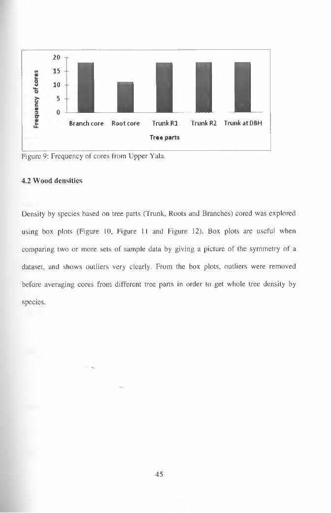
20
ou
c<u3cr
15
10 Li l l iBranch core Root core Trunk R1 Trunk R2 Trunk at DBH
Tree parts
Figure 9: Frequency of cores from Upper Yala.
4.2 Wood densities
Density by species based on tree parts (Trunk, Roots and Branches) cored was explored
using box plots (Figure 10, Figure 11 and Figure 12). Box plots are useful when
comparing two or more sets of sample data by giving a picture of the symmetry of a
dataset, and shows outliers very clearly. From the box plots, outliers were removed
before averaging cores from different tree parts in order to get whole tree density by
species.
45

Figure 10: Box plot of wood density by species based on trunk cores.
SpeclnAcacia meaman
Bndelia micranthaC w breium mpllp
Cupressus lusitanicaEucalyptus camalduiaosia
Eucalyptus grands Eucalyptus sahgna
Ficus sooQravtllee njbvsla Hanjngana madagascanensu
Jacaranda mimostfolia Mangifara indica Mark ham i a lutea Pmnus atncana
Syiygtum cordatum Svzvgium cvmtmt
Tnlapisium madogascanensis -
Note: Numbers besides boxes show outliers0« 97
Density (g/cmA3)
Figure 11: Box plot of wood density by species based on branch cores.

SptciesAcacia maamsn
Combratum mo/ta Cuprassus lusitamca
Eucalyptus camaldulansis Eucalyptus grants Eucalyptus saligna
Ficus spp Gravillea robosta
Harungana madagascanansis Jacaranda mimosifolia
Mangifara rn tca Markhamia lutes
Parsaa am an can a Prunus afncana
Syrygium cordatum Syzygium cumtnn
Tnlapisium madagascanansis
Note: Numbers besides boxes show
Figure 12: Box plot of wood density by species based on Root cores.
-cm
ID
cm
JD-
c m- n — f
(— r
TT“ oJ o' ■7 ;------- ?!------- ?■outliers Densit>- (g/cmA3)
4.3 Whole tree density
Before averaging the densities, means of tree parts were separated using Tukey's mean
separation (Table 10) using GenStat Statistical software (12th edition); The means were
not significantly different at p=0.05. Whole tree densities of species from the three
blocks calculated from carpenter’s auger method are summarized in table 11.
Table 10: Tukey's mean separation of tree parts
Tree part MeanRoot core V .' r 0.4877Trunk R2 0.5295Trunk at DBH 0.5359Trunk R1 0.5430Branch core 0.5445Note: Means are not significantly different at p=0.05
47

Table 11: Whole tree densities of species from the Yala Basin
Species TS Tc Mean Min Max Variance S.d(gem'3) (gem'3) (gem'3)
Acacia mearnsii 7 31 0.66 0.47 0.81 0.01 0.08Bridelia micrantha 2 7 0.38 0.22 0.55 0.02 0.13Combretum molle 1 5 0.66 0.58 0.70 0.00 0.05Croton macrostachyus 2 3 0.44 0.38 0.56 0.01 0.11Cupressus lusitanica 5 18 0.48 0.36 0.66 0.01 0.09Eucalyptus camaldulensis 28 108 0.51 0.30 0.79 0.01 0.11Eucalyptus grandis 10 37 0.47 0.22 0.75 0.01 0.12Eucalyptus saligna 2 5 0.34 0.17 0.45 0.01 0.11Ficus spp 2 5 0.44 0.28 0.53 0.01 0.10Grevillea robusta 19 27 0.62 0.52 0.72 0.00 0.05Harungana 2 4 0.47 0.45 0.49 0.00 0.02madagascariensis Jacaranda mimosifolia 6 10 0.47 0.35 0.63 0.01 0.09Mangifera indica 24 35 0.57 0.40 0.71 0.01 0.08Markhamia lutea 13 29 0.41 0.20 0.69 0.02 0.13Persea americana 3 5 0.44 0.42 0.48 0.00 0.02Prunus africana 14 16 0.74 0.67 0.79 0.00 0.04Spathodea campanulata 1 3 0.43 0.28 0.52 0.02 0.13Syzygium cordatum 7 10 0.76 0.68 0.79 0.00 0.04Syzygium cuminii 6 10 0.56 0.40 0.77 0.02 0.13Trilepisiummadagascariensis
3 5 0.52 0.45 0.68 0.01 0.09
Key: SD= standard deviation, TC= number of cores from each species, TS= Totalnumber of species
A total of 373 cores from three blocks were used for wood density estimation after
removing all the outliers; out of 404 core samples 31 outliers were removed from which
root cores contained the. highest number of outliers followed by branch core, indicating a
possibility of a problem with branch and root coring during samples collection. Trunk
had the least number of outliers.
3The densities were in the range of 0.34-0.75 gem" with an average mean value of 0.55
gem . Eucalyptus saligna was found with the lowest density value of 0.34 gem while
48

Syzygium cordatum had the highest density value of 0.75 gem'3. Within the same genus
of Eucalyptus, density values ranged from 0.51-0.34 gem' with Eucalyptus
camaldulensis having the highest density value followed by Eucalyptus grandis at 0.47 g
cm'3.
A study by Rueda and Williamson, (1992) showed that pioneer trees grow quickly at
first, producing low-density wood, and later add structural support by adding a shell of
harder wood. The controlling factor for adding the harder wood is the age of the tree,
rather than the diameter (De Castro et al., 1993).
4.4 Interactions between densities with species and tree parts
The Interactions between densities with species and tree parts showed significant effect
with F<0.001 for species as shown in table 12. However, there was no significance
difference in density between tree parts and species.
Table 12: Interactions between densities with tree species and tree parts.
Change DF SS MS Fpr+ Species 20 3.308752 0.165438 <0.001+ Tree parts 7 0.112910 0.016130 0.128+ Species. Tree parts 69 0.504632 0.007314 0.934Residual 276 2.735716 0.009912Total -312 6.662010 0.017909Key: ms= means standard error, ss=sum of squares, DF= degrees of freedom
4.5 Calculated and reported densities
The reference Global Wood Density database (GWD), which has wood densities for
8412 species from around the world (Flores and Coomes, 2010), and the African wood
49

density database (Carsan et al., 2012) provided data for comparison with the calculated
density values using different methods. Wood densities of similar species reported from
tropical Africa encountered in these databases were averaged, but since these densities
are reported in units of mass of wood at 12% moisture content per unit of volume at 12%
moisture content, a correction to equivalent oven dry densities was done using a
calibration equation developed by Reyes et al. (1992) by multiplying reported values by
0.88. The databases provided an opportunity for comparison between the calculated
density values and the reported densities (Table 13).
50

Table 13: Calculated densities and reported densities.
Species C.dReported densities (gem'3) by regionsT. Africa Asti S-E Asia China SA India
Acacia mearnsii 0.66 - 0.66 - - - -Bridelia micrantha 0.38 0.44-0.58 0.50 - -Combretum molle 0.66 0.79 - - - - -Croton macrostachyus 0.44 0.45-0.52 - - - - -Cupressus lusitanica 0.48 0.39 - - - - -Eucalyptus camaldulensis 0.51 - 0.48-0.97 - 0.59 - -Eucalyptus grandis 0.47 - 0.63-0.66 - - - -Eucalyptus saligna 0.34 - 0.68-0.86 - - - -Ficus spp 0.44 - - - - -Grevillea robusta 0.62 0.51-0.516 - 0.5 - 0.64Harungana madagascariensis 0.47 0.47 - 0.47 - - -Jacaranda mimosifolia - - - - -
0.47Mangifera indica 0.57 0.54 - 0.52 - - 0.68Markhamia lutea 0.41 0.47 - - -Persea americana 0.44 0.52 - - - 0.6Prunus africana 0.74 0.77 - - - - -Spathodea campanulata 0.43 - - - - - -Syzygium cordatum 0.76 0.62 - - - - -Syzygium cuminii 0.56 - - - 0.63 0.76Trilepisium madagascariensis 0.52 0.50 - - - - -Key: Cd= calculated density, T. Africa=Tropical Africa, Asti = Australia, SA=South America,-no reported value
51

From these two databases not all species were reported and the density of Ficus spp was
not reported in the global data base; however most of the values reported were within the
range of those calculated using the carpenter’s auger method.
4.6 Carbon and nitrogen analyses
Total carbon and nitrogen concentrations determined using thermal oxidation are
summarized in tables 14 and 15. Measured carbon and nitrogen values in percentage
were converted to contents (gem3) by dividing by 100 then multiplying by the
corresponding species density.
52

Table 14: Measured carbon (%) and Carbon contents (gem 3).
Species TS Nc Mean Min Max Variance S.d C(gcm'J)Acacia mearnsii 27 24 48.08 47.36 48.61 0.14 0.37 0.32
Bridelia micrantha 3 7 45.02 43.95 45.99 0.40 0.63 0.17Combretum molle 3 5 46.80 45.49 48.05 0.86 0.93 0.31Croton macrostachyus 1 3 44.13 43.95 44.44 0.07 0.27 0.20Cupressus lusitanica , 9 15 47.21 46.19 48.67 0.44 0.67 0.23Eucalyptus camaldulensis 63 116 46.50 44.61 48.54 0.74 0.86 0.24Eucalyptus grandis 10 37 48.37 46.90 50.31 0.64 0.80 0.23Eucalyptus saligna 6 6 47.97 45.13 49.41 2.72 1.65 0.17Ficus spp 1 5 47.80 46.92 48.51 0.33 0.57 0.21Grevillea robusta 5 22 49.17 47.31 50.68 0.78 0.88 0.30Harungana madagascariensis 1 5 48.51 47.53 49.27 0.46 0.68 0.23Jacaranda mimosifolia 2 11 48.60 46.04 50.02 1.61 1.27 0.23Mangifera indica 7 36 47.19 45.60 48.60 0.45 0.67 0.27Markhamia lutea 9 30 48.77 47.11 50.72 0.78 0.88 0.20Persea americana 2 6 47.52 46.88 48.03 0.18 0.43 0.21Prunus africana 16 20 47.93 46.50 49.14 0.50 0.71 0.35Spathodea campanulata 1 3 47.43 46.25 48.46 1.24 1.11 0.20Syzygium cordatum 2 9 48.23 47.31 49.08 0.35 0.59 0.37Syzygium cuminii 2 10 48.56 45.61 51.26 2.06 1.43 0.27Trilepisium madagascariensis 1 5 47.41 46.64 47.84 0.25 0.50 0.25
-- -̂--------------Key: SD= standard deviation, Nc=number of cores from each species, TS= Total number of trees, C=carbon content in gem 3.
53

Table 15: Measured Nitrogen (%) and Nitrogen contents (gem" ).■5
Species TS Nc Mean Min Max Variance S.d. N(gcm‘J)
Acacia mearnsii 27 35 0.27 0.14 0.38 0.0049 0.07 0.0018Bridelia micrantha 3 7 0.23 0.21 0.25 0.0001 0.01 0.0009Combretum molle 3 3 0.29 0.28 0.31 0.0004 0.02 0.0019Croton macrostachyus 1 3 0.27 0.26 0.28 0.0001 0.01 0.0012Cupressus lusitanica 9 18 0.22 0.13 0.28 0.0016 0.04 0.0011
Eucalyptus camaldulensis 63 118 0.22 0.11 0.34 0.0016 0.04 0.0011
Eucalyptus grandis 19 31 0.20 0.11 0.42 0.0036 0.06 0.0009Eucalyptus saligna 2 6 0.21 0.18 0.26 0.0009 0.03 0.0007Ficus spp 2 5 0.30 0.29 0.31 0.0001 0.01 0.0013Grevillea robusta 19 28 0.23 0.09 0.35 0.0025 0.05 0.0014Harungana madagascariensis 2 5 0.25 0.23 0.28 0.0004 0.02 0.0012Jacaranda mimosifolia 6 11 0.30 0.25 0.36 0.0009 0.03 0.0014Mangifera indica 24 37 0.24 0.11 0.37 0.0016 0.04 0.0014Markhamia lutea 13 28 0.34 0.24 0.43 0.0016 0.04 0.0014Persea americana 3 7 0.25 0.21 0.31 0.0016 0.04 0.0011
Prunus africana 16 20 0.21 0.14 0.29 0.0009 0.03 0.0016Spathodea campanulata 1 3 0.24 0.23 0.26 0.0004 0.02 0.0010Syzygium cordatum 7 10 0.28 0.24 0.31 0.0004 0.02 0.0021Syzygium cuminii 6 9 0.24 0.16 0.36 0.0036 0.06 0.0014Trilepisium madagascariensis 3 5 0.29 0.21 0.32 0.0025 0.05 0.0015Key: SD= standard deviation, Nc=-number of cores from each species, TS-= Total number of trees, N=Nitrogen content in gem"’
54
Species mean carbon values ranged from 44 to 49% and 0.17 to 0.36 g cm 1 for carbon
content. The carbon and nitrogen values were in agreement with previously reported
range, species variation in total C was statistically significant (P<0.001), with values
ranging from 44.13% in Croton macrostachyus to 49.17% in Grevillea robusta (Table
14).
Carbon variation and measurement error was relatively low, with an average standard
deviation of 0.79%. All the twenty species examined had an average percentage C of
47.56%, significantly lower than 50% default carbon value. Thus, this variation with thee
often assumed default value of 50% C in wood could lead to an over estimation of tree C
stocks but still provides a rough estimate of carbon biomass.
Most species deviated from this estimate by between 1-4% using 50% as reference value.
Croton macrostachyus an indigenous species in the area showed high deviation of 4%.
However, similar deviations of 2-3% among conifers were reported by Thomas and
Malczewski (2007). For conifers, 2-3% deviation resulted in 4-6% bias in carbon stock
assessments (Thomas and Malczewsk,i 2007).
The reported deviation of 1-4% in this study could result in about 2-8% bias in carbon
stock assessments in tropical agricultural landscape. A 1% difference in carbon content
conceivably could have a significant impact on wood and pulp industries in relation to
allocation of carbon credits within the context of Kyoto Protocol (Lamlom and Savidge,
2003).
The total nitrogen concentration among different species ranged from 0.34% in
Markhamia lutea to 0.2% in Eucalyptus grandis. Elemental nitrogen in plants has been
55

reported by Pettersen (1984) to be in the range of 0.1-0.5%. The twenty species had a
mean value of 0.25% and range of 0.17 to 0.36 gem '3 for nitrogen content.
4.7 Correlation between wood density, carbon and nitrogen contents
Wood density values were positively correlated with carbon content (r = 0.995) and
nitrogen content (r = 0.849), these were supported by Pearson correlation matrix (Table
16 and Figure 13).
Table 16: Pearson correlation between density, carbon and nitrogen.
Variables ------------------------ 3----Density(gcm’ ) Carbon(gcm 3)
Carbon (gem' ) 0.995
Nitrogen(gcm 3) 0.849 0.844
Key: Values in bold are significantly different with a significance level alpha p < 0.05.
In general, there was a very strong positive correlation between wood density, carbon
and nitrogen, all at p<0.0001. These correlations are important in carbon pool assessment
and are in agreement with Dietz (2007) that a better understanding of wood density
values can reduce the error of carbon pool estimation.
The higher the density values the higher the C and N contents (Figures 13 and 14).
Hacke et al. (2001) showed that wood density correlates positively with carbon and■V
concluded that high wood density is advantageous for survival in dry climates and may
aid in the transport of liquids in dry conditions. However, this may suggest the
adaptation of these species to the Yala basin given that wood tends to be chemically as
well as anatomically unique for individual species. Therefore, it would be reasonable to
56
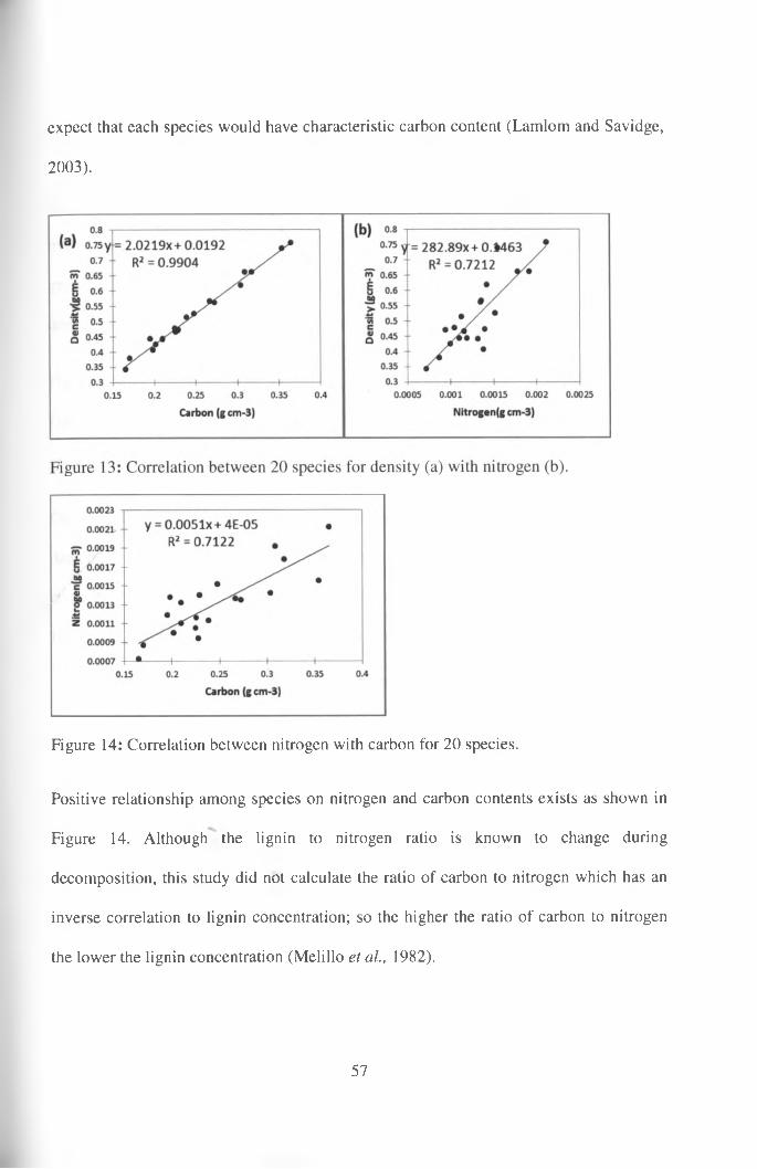
expect that each species would have characteristic carbon content (Lamlom and Savidge,
2003).
Figure 14: Correlation between nitrogen with carbon for 20 species.
Positive relationship among species on nitrogen and carbon contents exists as shown in
Figure 14. Although the lignin to nitrogen ratio is known to change during
decomposition, this study did not calculate the ratio of carbon to nitrogen which has an
inverse correlation to lignin concentration; so the higher the ratio of carbon to nitrogen
the lower the lignin concentration (Melillo et al., 1982).
57

4.8 Species variation with wood density, carbon and nitrogen
High wood density is a characteristic of slowly growing species, found in dry soils or in
nutrient-poor soils (Preston et a i, 2006; Muller-Landau, 2004) than similar shrub-like
growth (Preston et al., 2006). Syzygium cordatum and Prunus africana had highest
densities (Note: Size of points indicates increasing densities.
Figure 15). S. cordatum is described in ICRAF database as one of southern Africa's
fastest growing trees (up to lm/year) while Prunus africana is described as a slow
growing species.
Growing the same species in different geographical locations can result in readily
detectable differences in wood properties. Some softwood species showed higher carbon
content; which was attributed to the fact that softwoods have approximately 10% more
lignin than hardwoods (Lamlom and Savidge, 2003).
58

0.4
0.35(a)
< 0
m 0.3
i| «j 0.2
0.15
• • 9
0.10.3 0.35 0.4 0.45 0.5 0.55 0.6
D«nsity(gcm-3)
—I-------- 1-------- 1-------- 10.65 0.7 0.75 0.8
0.0025
0.002
3C 0.0015
§u±fz0.001
0.0005
(b)
9
0.35 0.4 0.45
Acacia mearnsii Combretum molle Cupressus lusitanica Eucalyptus grandis Ficus sppHarungana madagascariensis Mangifera indica Persea americana
0.5 0.55 0.6
Density (gcm-3)
0.65 0.7 0.75
Bridelia micrantha Croton macrostachyus Eucalyptus camaldulensis Eucalyptus saligna Grevillea robusta Jacaranda mimosifolia Markhamia lutea Prunus africana
0.8
Note: Size of points indicates increasing densities.
Figure 15: Species-specific density values with (a) carbon (b) nitrogen
The kind of positive relationship (R2=0.99) between wood density and carbon content
(Note: Size of points indicates increasing densities.
Figure 15) are practically useful for C stock estimation since determination of carbon is
relatively difficult and expensive (Elias and Potvin, 2003).

Wood density has been proposed as a good proxy to C estimation in tropical trees.
Findings by Elias and Potvin, (2003) showed strong relationships between C and wood
density (R2 = 0.86). Similar relationship was reported by Thomas, (1996) and Muller-
Landau, (2004) in diverse forest ecosystems. Theoretically slow-growing species often
contain high C compounds (e.g., lignins, polyphenolic compounds), whereas fast
growing species contain low C compounds (e.g., alkaloids, phenolic glycosides,
cyanogenic glycosides).
Schlesinger (1991) reported that C content of biomass is almost always found to be
between 45% and 50% (by oven-dry mass) and thus, the carbon content of vegetation
may be estimated by simply taking a fraction of the biomass by:
C = 0 .4 7 5 x 5 ..................................................................................................................Eq 10
Where, C is carbon content by mass, and B is oven-dry biomass.
4.9 Indigenous and exotic trees carbon storage
Relationship among the twenty tree species collected from Yala basin was explored by
cluster analysis based on Euclidean distance under taken using an un-weighted pair
group method with arithmetic averaging. The species were divided into indigenous and
exotic (Table 18), proximity matrix showed four major clusters (Figure 16); the
clustering was based on species carbon and their distances shown in Table 18.

0 1 2 3 4 0 1 2 3 4
Dissimilarity Dissimilarity
Figure 16: Dendogram based on Euclidean distance for 20 tree species.
The cluster numbers in the dendogram corresponds to species as given in the key of table
18 and their corresponding types. However, the cluster distances are given in Table 17.
Table 17: Distances between four clusters among 20 species from Yala basin.
Cl(Indigenous) C2 (Indigenous) C3 (Exotic)Cl (Indigenous)C2 (Indigenous) 3.210C3 (Exotic) 1.040 2.170C4 (Exotic) 0.940 4.150 1.980
The mean carbon values for indigenous cluster 1 and 2 were 48.23% and 45.02%
respectively. While the exotic clusters 3 and 4 had carbon values of 49.17% and 47.19%
respectively.
61
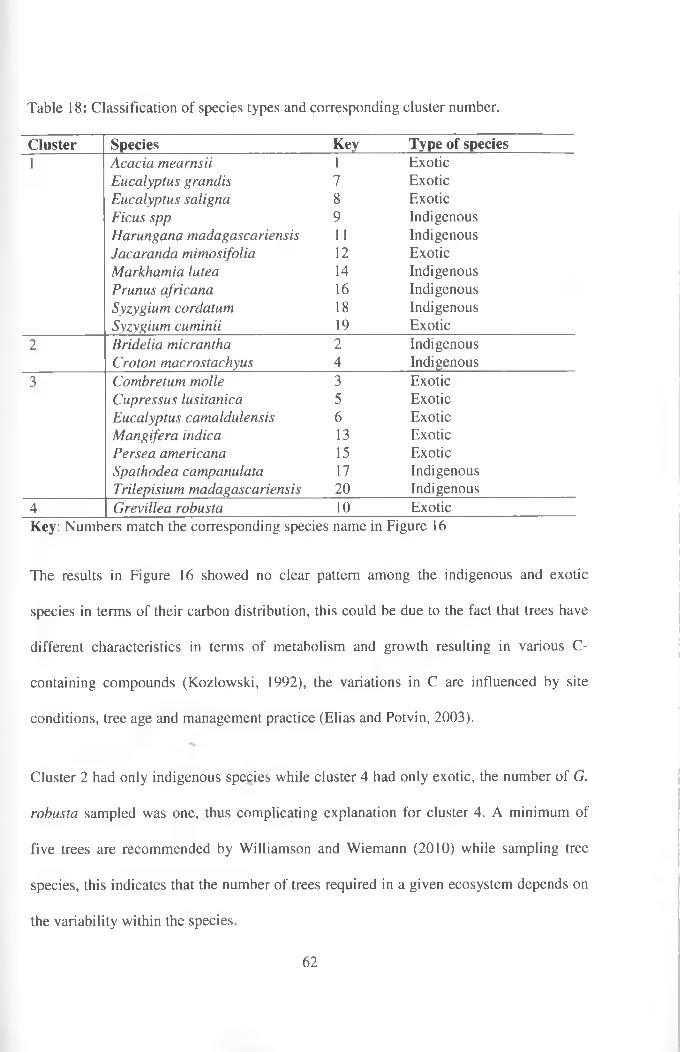
Table 18: Classification of species types and corresponding cluster number.
Cluster Species Key Type of species1 A ca c ia m earn sii 1 Exotic
E u ca lyp tu s g ra n d is 7 ExoticE u ca lyp tu s sa lig n a 8 ExoticF icu s sp p 9 IndigenousH aru n gan a m a d a g a sca rien sis 11 IndigenousJ a ca ra n d a m im osifo lia 12 ExoticM arkh am ia lu tea 14 IndigenousPrunus a frican a 16 IndigenousS yzyg iu m corda tu m 18 IndigenousS yzyg iu m cum inii 19 Exotic
2 B rid e lia m icran th a 2 IndigenousC ro ton m acro sta ch yu s 4 Indigenous
3 C om bretu m m olle 3 ExoticC u p ressu s lu sitan ica 5 ExoticE u ca lyp tu s ca m a ld u len sis 6 ExoticM an gifera indica 13 ExoticP erse a am erica n a 15 ExoticS p a th o d ea cam pan u la ta 17 IndigenousT rilep isiu m m a d a g a sca rien sis 20 Indigenous
4 G rev ille a robu sta 10 ExoticKey: Numbers match the corresponding species name in Figure 16
The results in Figure 16 showed no clear pattern among the indigenous and exotic
species in terms of their carbon distribution, this could be due to the fact that trees have
different characteristics in terms of metabolism and growth resulting in various C-
containing compounds (Kozlowski, 1992), the variations in C are influenced by site
conditions, tree age and management practice (Elias and Potvin, 2003).
Cluster 2 had only indigenous species while cluster 4 had only exotic, the number of G.
rob u sta sampled was one, thus complicating explanation for cluster 4. A minimum of
five trees are recommended by Williamson and Wiemann (2010) while sampling tree
species, this indicates that the number of trees required in a given ecosystem depends on
the variability within the species.
62
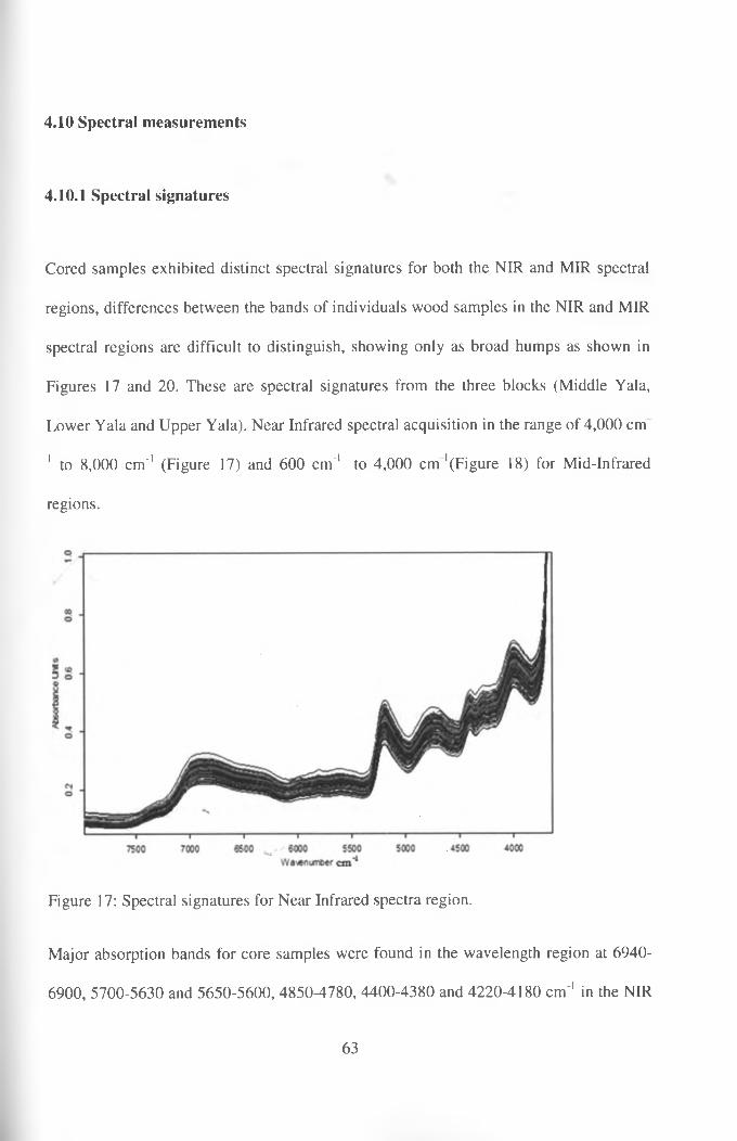
4.10 Spectral measurements
4.10.1 Spectral signatures
Cored samples exhibited distinct spectral signatures for both the NIR and MIR spectral
regions, differences between the bands of individuals wood samples in the NIR and MIR
spectral regions are difficult to distinguish, showing only as broad humps as shown in
Figures 17 and 20. These are spectral signatures from the three blocks (Middle Yala,
Lower Yala and Upper Yala). Near Infrared spectral acquisition in the range of 4,000 cm
1 to 8,000 cm'1 (Figure 17) and 600 cm '1 to 4,000 cm '(Figure 18) for Mid-Infrared
regions.
Figure 17: Spectral signatures for Near Infrared spectra region.
Major absorption bands for core samples were found in the wavelength region at 6940-
6900, 5700-5630 and 5650-5600, 4850-4780, 4400-4380 and 4220-4180 cm '1 in the NIR
63

spectral region. Bonds with more s character absorb at high frequency, Sp1 (C-H) just
below 3000 cm '1 to the right, SP2 (C-H) just above 3000 cm '1 to the left and SP (C-H) at
3300 cm 1. O-H stretch of carboxylic acid (COOH) absorbs broadly due to strong
hydrogen bonding at 2500cm'1. Also notable peak around 5650-5600 cm '1 could be as a
possible result of -CH3 stretch in first harmonic region and various functional groups
present in different tree species of wood samples, specific absorption bands are as shown
in table 19.
Table 19: Specific absorption bands in near Infrared spectra of wood cores.
Wavenumber (cm 1) ChemicalGroup
Characteristicvibration
Spectral region
12000-9000 Noisy region 3rd harmonic9350-9220 -CH andC-C Stretch Combination8850-8770 Aromatic 2nd harmonic
8700-8580;8840-8370 and 8400-8330
-CH3 Stretch 2nd harmonic
7170-7020 -OH Bend 1st harmonic7090-7040 and 6940-6900 -CH and CH Stretch and bend Combination5950-5920 Aromatic Inharmonic5850-5870;5700-5630 and 5650-5600
-CH3 Stretch 1st harmonic
4850-4780 -OH Stretch and bend Combination4400-4380 CH- Stretch and bend Combination4220-4180 -OH Stretch 2nd harmonicSource: Banwell (1983)
In the spectral signatures in MIR region (Figure 18), dominant absorption features were
observed in the following region: 3400, 1750-1600, 2970, 2250, 2220, 1750-1600 and
1200-1000 cm '1 suggesting the following functional groups; -NH2, -CH3, -C=N, -C=C,
>C=Q and from 1200-1000 cm'1; -C-C-, -C-N and -C-0-.
64

3500 3000 2500 2000 1500 1000W avenum ber cm -1
Figure 18: Full range spectral signatures for mid-infrared spectra region.
The distinct fingerprint region of Mid-Infrared from 1200-600 cm '1 is hard to resolve but
is useful since different species have different compounds with distinct fingerprint
signatures. Table 20 has characteristic stretching frequencies for some of molecular
groups around MIR region. The finger print region shows both the skeletal vibrations-
involving all atoms and the characteristic group vibrations which only involves small
portion of the molecule, with the remainder being more or less stationary. Skeletal■*>
frequencies are in the range of 1400-700 cm '1 and arise from linear or branched chain
structures (Banwell, 1983). The high peak around 1350 cm 1 is due to C-H and O-H
bending vibrations (Banwell, 1983).
65
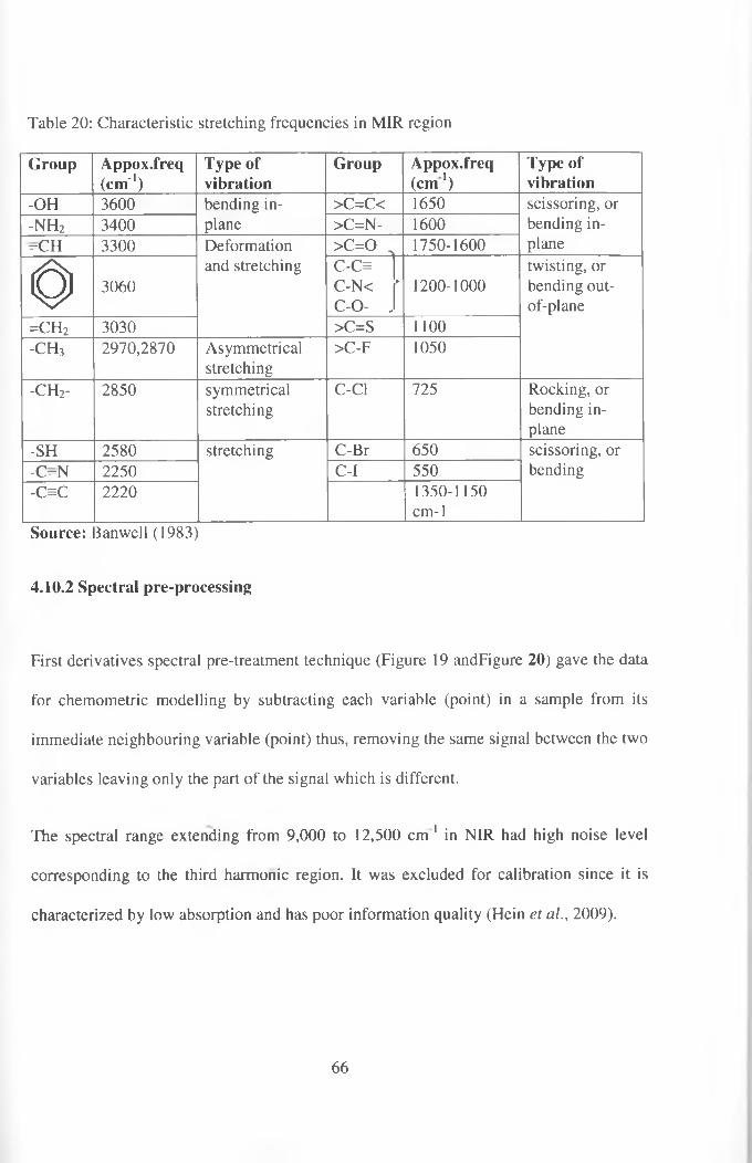
Table 20: Characteristic stretching frequencies in MIR region
Group Appox.freq(cm'1)
Type of vibration
Group Appox.freq(cm 1)
Type of vibration
-OH 3600 bending in- plane
>C=C< 1650 scissoring, or bending inplane
-n h 2 3400 >C=N- 1600=CH 3300 Deformation
and stretching> c= o „ 1750-1600
03060
C O C-N< ' C-O- .
1200-1000twisting, or bending out- of-plane
=c h 2 3030 >C=S 1100-c h 3 2970,2870 Asymmetrical
stretching>C-F 1050
-c h 2- 2850 symmetricalstretching
C-Cl 725 Rocking, or bending inplane
-SH 2580 stretching C-Br 650 scissoring, or bending-C=N 2250 C-I 550
-C=C 2220 1350-1150cm-1
Source: 3anwell (1983)
4.10.2 Spectral pre-processing
First derivatives spectral pre-treatment technique (Figure 19 andFigure 20) gave the data
for chemometric modelling by subtracting each variable (point) in a sample from its
immediate neighbouring variable (point) thus, removing the same signal between the two
variables leaving only the part of the signal which is different.
The spectral range extending from 9,000 to 12,500 cm 1 in NIR had high noise level
corresponding to the third harmonic region. It was excluded for calibration since it is
characterized by low absorption and has poor information quality (Hein et al., 2009).
66

c Raw spectrao
< 4000 5000 6000 7000 8000
Wavebands
c Derivative spectrao
< ' 4000 5000 6000 7000 8000
Wavebands
Figure 19: Reduced raw and first derivative of NIR spectra.
Hein et al., (2009) reported the application of spectral filter, exclusion of outliers and
selection of variables wavelengths as a way of improving statistics associated with
models. Similarly Jones et al., (2006) also reported improvement while studying basic
density of 120 samples of Pinus taeda. These findings demonstrated that application of
spectral data pre-treatment of the first derivative reduced the standard error of prediction
(SEP) but increased ratio performance deviation (RPD).
67

Raw spectra
? - p jO T -
Q. lf> _--------- 1---------- 1---------- 1---------- 1---------- 1---------- 1---------- rT
1000 1500
T
2000 2500
Wavebands
3000 3500 4000
Derivative spectra
Wavebands
Figure 20: Raw and first derivative of Mid-Infrared spectra.
4.10.3 Selected samples
The selected representative samples (Figure 21) were based on recorded NIR and MIR
spectral diversity using the Kennard-Stone algorithm and calculated from principal
component scores (PCs). The PCs approximates the original data to desired degree of
accuracy (Cozzolino el al., 2009), transforming a set of correlated variables into a** '
smaller number of uncorrelated variables called latent variables. Other different
calibration sets followed the same principle. The pictorial representation (Figure 21)
helps to visualise whether the selected samples are really representative.
68

6 0 -2 0 0 2 0 4 0 6 0 8 0PC1 explains 37 8 %
6 0 -2 0 0 2 0 4 0 6 0 8 0PC1 explains 37 8 %
6 0 -2 0 0 2 0 4 0 6 0 8 0PC1 explains 37 8 %
-4 0 -2 0 O 2 0 4 0PC3 explains 10 6 %
Figure 21: Selection based on 10% with red indicating selected samples
4.11 PLS Calibration
4.11.1 Developing a calibrations using all samples set
In this approach all the samples are used as the calibration set, expecting best calibration
thus, giving the best indication of the potential of mid-IR or NIR as useful tool for■v
determining physical and chemical composition (Bellon-Maurel and McBratney, 2011).w'
The calibration performance was low (Table 21, Figures 22 and 23) with low R2 values
both for MIR and NIR, making it virtually impossible for the calibration to determine
accurately the composition of new samples from their spectra alone.
69
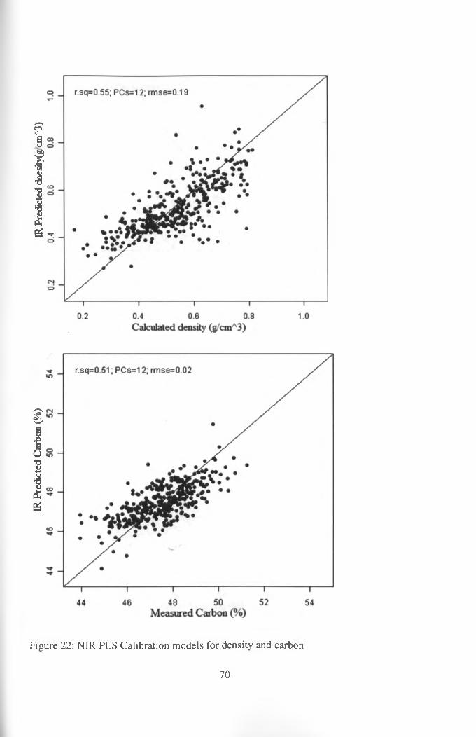
IR P
redi
cted
Car
bon
(%)
IR P
redi
cted
dne
sity(
g cin
A3)
Figure 22: NIR PLS Calibration models for density and carbon
70

IR P
redi
cted
Car
bon
(%)
DR P
redi
cted
den
sity
(g'c
mA3
)
Figure 23: MIR PLS Calibration models for density and carbon
71

The data presented in table 21 show that the Nir-IR calibrations in terms of R for WD
was fairer at (R2=0.55), while the rest were poor with R <0.50. Mid-IR calibrations were
not good either with nitrogen (R2=0.51) and the other properties having R2<0.50. With
only a few exceptions, calibrations based on Nir-IR spectra were better (larger R2 and
smaller RMSECV) than their MIR counterparts even after removing wavelengths
associated with CO2 region.
Table 21: Statistical summary of cross-validated calibration results using all samples as the calibration set
IR range n Property PCs R2 Bias RMSECVNIR 373 WD 12 0.55 -0.03 0.17
375 C 12 0.51 -3.48 12.59389 N 9 0.48 -0.04 0.09381 Cg 6 0.49 0.02 0.11380 Ng 9 0.38 -6E-05 6E-04
MIR 373 WD 6 0.42 -0.03 0.18375 C 8 0.49 -3.37 12.92389 N 9 0.51 -0.04 0.09381 Cg 6 0.43 0.02 0.11380 Ng 9 0.42 -4E-05 6E-04
Key: WD = wood density (gem'3), C =carbon (%), N = Nitrogen, Cg =carbon (gem'3), n=total number of samples after removal of outliers
The calculated principle components (PCs) were affected by various wave-lengths
attributable to various chemical structures and compounds (Chodak et al., 2007); PCs
reduced the data points describing the manipulated NIR /MIR spectra.
For wood density prediction using MIR spectra (90% Calibset), PCI was dominated by
absorption at 1890 and 700 cm '1, which may be attributed to COOH groups (Figure 24).
PC2 was affected mainly by absorption between 3,500 and 2,500 cm 1 (attributable to
CH3 groups) and PC3 by absorption at 3,670, 3,300, and 2,350 nm (attribued to CH2 and
CH3 groups).
72

Figure 24: Plot of factor loading values for the PCs for MIR spectra
From the means of these three methods (Table 22), predicted mean wood density values
from NIR and MIR was 0.527 gem'3 and 0.528 gem 3 while the calculated density was
0.59 gem'3. Mean carbon predicted was 47.58% (NIR), 47.59% (MIR) and laboratory
measured mean carbon value was 47.61%. Mean IR predicted nitrogen was 0.24% (NIR)
and 0.24% for MIR, while laboratory determined value was 0.28%. Predicted Carbon
(gem'3) from NIR and MIR spectra had the same mean values of 0.28 gem'3, but low
mean laboratory values of 0.24 gem'3. Mean nitrogen in (gem'3) was the same for both
the IR and laboratory measured values (0.0014 gem' ). The standard deviation of these
properties were small given that the predictions were from different ranges of
wavelengths (NIR and MIR) compared to the values obtained by laboratory
measurement.
73
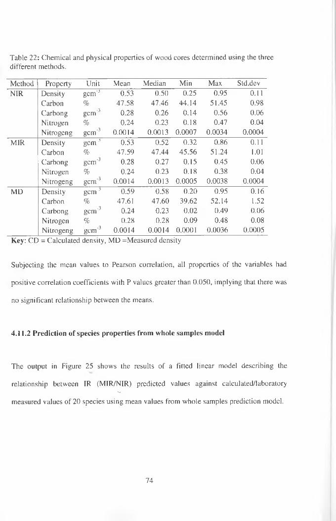
Table 22: Chemical and physical properties of wood cores determined using the three different methods.
Method Property Unit Mean Median Min Max Std.devNIR Density gem'3 0.53 0.50 0.25 0.95 0.11
Carbon % 47.58 47.46 44.14 51.45 0.98Carbong gem 3 0.28 0.26 0.14 0.56 0.06Nitrogen % 0.24 0.23 0.18 0.47 0.04Nitrogen g gem-3 0.0014 0.0013 0.0007 0.0034 0.0004
MIR Density gem"3 0.53 0.52 0.32 0.86 0.11Carbon % 47.59 47.44 45.56 51.24 1.01Carbong gem'3 0.28 0.27 0.15 0.45 0.06Nitrogen % 0.24 0.23 0.18 0.38 0.04Nitrogeng gem"3 0.0014 0.0013 0.0005 0.0038 0.0004
MD Density gem'3 0.59 0.58 0.20 0.95 0.16Carbon % 47.61 47.60 39.62 52.14 1.52Carbong gem"3 0.24 0.23 0.02 0.49 0.06Nitrogen % 0.28 0.28 0.09 0.48 0.08Nitrogeng gem"3 0.0014 0.0014 0.0001 0.0036 0.0005
Key: CD = Calculated density, MD =Measured density
Subjecting the mean values to Pearson correlation, all properties of the variables had
positive correlation coefficients with P values greater than 0.050, implying that there was
no significant relationship between the means.
4.11.2 Prediction of species properties from whole samples model
The output in Figure 25 shows the results of a fitted linear model describing the
relationship between IR (MIR/NIR) predicted values against calculated/laboratoryv '
measured values of 20 species using mean values from whole samples prediction model.
74

Calculated carbon (g/cm,'3)
• NIR * MIR
Calculated Nitrogen (g/cm/'3 )
• NIR * M IR
44.00 46.00 48.00 50.00Measured carbon (% )
• NIR * M IR
Measured Nitrogen (%)
• NIR K MIR
K E YA=Density (g/cmA3) B=Carbon (%) C=Nitrogen (%) D=Carbon (g/cmA3) E=Nitrogen (g/cmA3)
Figure 25: A model between IR predicted and measured values (all samples)
These linear models shows that when the values averaged to the species level the
prediction is much better than the individual core models, an indication that large within
species variations exist that cannot be predicted using IR. But in general all other
properties were well predicted using NIR with both models showing statistically
75

significant relationship. The nitrogen content both calculated (gem'3) and measured (%)
had good correlation with NIR predicted values with R2 of 0.83. While MIR gave R2 of
0.62 and 0.80 respectively. For NIR, carbon both calculated (gem-3) and measured (%)
gave R2 value of 0.66 and 0.82 respectively, and 0.57 and 0.72 respectively for MIR. In
NIR the predicted values gave a correlation coefficient greater than 0.080, indicating
strong relationship.
4.11.3 Calibration and validation using 50/50 split
Table 23 lists performance details of the analysis of PLS models for wood properties. For
carbon, the calibration model performed better than the initial model developed using the
entire samples, with the R2 value improving from 0.51 to 0.75 for calibration, and 0.31
for validation in NIR region (Figure 27).
The R-Square validation set explains 30.68% of the variability in predicted values, while
the correlation coefficient equals 0.55, indicating a moderately strong relationship
between the variables. While for MIR R2 value improved from 0.45 to 0.53 for
calibration, and 0.40 for validation (Figure 26). The validation model explains 40.43% of
the variability in predicted set.
The correlation coefficient equals 0.64 indicates a moderately strong relationship
between the variables, other properties were poorer with R2<50 in calibration sets. For
density, nitrogen model had similar performance, while the SECV showed a small
increase in the 50/50 model.
76

44 46 48 SO SJ M
Measured Carbon (%)Figure 26: MIR PLS models for carbon
Measured Carbon (%)Calibration and (B) validation.
Figure 27: NIR PLS models for carbon (A) Calibration and (B) validation.
77

Table 23: Cross-validated calibration and Independent validation results for NIR and MIR region of spectra based on 50/50 split.
Calibration ValidationIR n Prop R2 RM PCs n Prop R2 Bias RMSEPrange erty SECV ertyNIR 187 WD 0.24 0.21 2 186 WD 0.19 -0.03 0.18
186 C 0.75 0.02 12 187 C 0.31 -3.07 12.71195 N 0.07 0.22 2 194 N 9E-06 -0.04 0.08191 Cg 0.33 0.23 3 190 Cg 0.18 0.01 0.10190 Ng 0.11 0.33 2 190 Ng 0.05 0.000 0.001
MIR 187 WD 0.39 0.19 3 186 WD 0.31 -0.04 0.19186 C 0.53 0.02 7 187 C 0.40 -3.50 12.95195 N 0.32 0.2 3 194 N 0.03 -0.04 0.08191 Cg 0.39 0.23 3 190 Cg 0.01 0.01 0.11190 Ng 0.31 0.3 3 190 Ng 0.28 0.000 0.001
Key: WD = wood density (gem'3), C =carbon (%), N = Nitrogen, Cg =carbon (gem'3), n=total number of samples
4. 11.4 Prediction of species properties using 50/50 split model
Statistical summary of predictions developed using 50/50 split is shown in table 24; the
mean values were regressed against measured values (Figure 28). At 95.0% confidence
level, the predictions developed using MIR was generally better than NIR; density
R2=0.51(MIR) and R2=0.46 (NIR), carbon (%) R2=0.60 (MIR) and R2=0.48 (NIR),
nitrogen (%) R2=0.66 (MIR) and R2=0.02 (NIR), carbon (gem'3) and nitrogen (gem'3)
R2<0.50 for both MIR and NIR.
78
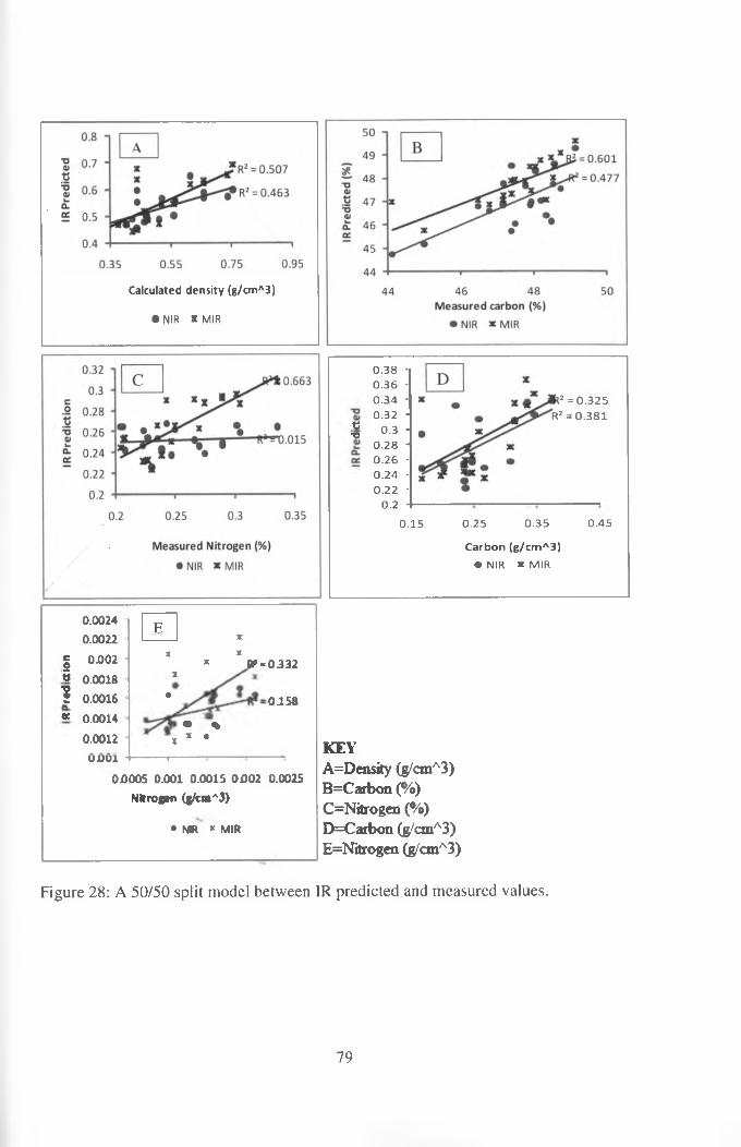
Calculated density (g/cmA3)
• N IR X M IR
t!T3
0 .3 8 ■ 0 .3 6 ■ 0 .3 4 ■ 0 .3 2 ■
0 .3 ■ 0 .2 8 ■ 0 .2 6 ■ 0 .2 4 -
0.22 ■
0.2 ■
2 = 0 .3 2 5
R2 = 0 .3 8 1
0 .1 5 0.2 5 0 .3 5 0 .45
C arbon (g/cm A 3)
• NIR * M IR
0 .0024F
0 .0022 X
£ 0 0 0 2 ■ 2
X X
* £P = 0 3 3 2« 0 .0018 X
I 0 .0 0 1 6 •0 .1 5 8
“ 0 .0014• %
0 .0012 X* •
U jU U I *
0 0 0 0 5 0 .0 0 1 0 .0 0 1 5 0 0 0 2 0 .0025
N itrogen (g /c m A3 )
• NIR * MIR
K E YA=Density (g/cmA3) B=Carbon (%) C=Nitrogen (%) D=Carbon (g/cmA3) E=Nitrogen (g/cmA3)
Figure 28: A 50/50 split model between IR predicted and measured values.
79

Table 24: Summary statistics of predicted values using 50/50 split mode
Property Mean Min Max S.D C.V(% )Density (gem'-5) 0.52 0.34 0.76 0.12 0.23MIR Predicted 0.55 0.44 0.69 0.08 0.15NIR Predicted 0.53 0.45 0.65 0.05 0.10Carbon (%) 47.56 44.13 49.17 1.24 0.03MIR Predicted 47.80 45.74 49.58 0.93 0.02NIR Predicted 47.02 44.71 49.26 1.17 0.02Nitrogen (%) 0.25 0.20 0.34 0.04 0.15MIR Predicted 0.26 0.22 0.31 0.03 0.10NIR Predicted 0.25 0.23 0.27 0.01 0.05Carbon (gem'3) 0.26 0.17 0.38 0.06 0.23MIR Predicted 0.29 0.23 0.37 0.05 0.16NIR Predicted 0.28 0.22 0.34 0.04 0.14Nitrogen (gcm'J) 0.001 0.001 0.002 0.000 0.27MIR Predicted 0.002 0.001 0.002 0.000 0.20NIR Predicted 0.001 0.001 0.002 0.000 0.11Key: Min=Minimum, Max=maximum, S.D=Standard deviation, C.V=Coefficient of variation
The properties of the variables had positive correlation coefficients with P > 0.05, except
in the density estimation where P < 0.05.
4.11.5 Varying percentages of Calibration set
Table 25 and 27 shows results for calibration sets of 10%, 20%, 30%, 50%, 60%, 70%,
80% and 90% for the properties in both NIR and MIR region. While tables 26 and 28
shows the independent validations sets. Coefficient of determination (R ), bias and root
mean square error of prediction (RMSEP) shows the predictive performance for cross-
validated calibrations results and independent validations.
80

Table 25: NIR Cross-validated calibration results.
Calibset
Property R" PCs RMSECV
Calibset
Property ~R2 PCs RMSECV
Calibset
Property R2 PCs RMSECV
10% WD 0.27 1 0.19 40% WD 0.24 2 0.21 70% WD 0.33 4 0.210% C 0.42 2 0.02 40% C 0.75 12 0.02 70% C 0.76 15 0.0110% N 0.35 2 0.19 40% N 0.13 2 0.21 70% N 0.03 1 0.2210% Cg 0.13 h 0.19 40% Cg 0.21 2 0.24 70% Cg 0.48 10 0.210% Ng 0.03 1 0.3 40% Ng 0.03 1 0.33 70% Ng 0.39 10 0.2820% WD 0.5 3 0.17 50% WD 0.24 2 0.21 80% WD 0.52 12 0.1720% C 0.53 2 0.02 50% C 0.75 12 0.02 80% C 0.37 4 0.0220% N 0.45 3 0.18 50% N 0.07 2 0.22 80% N 0.31 7 0.2120% Cg 0.36 3 0.2 50% Cg 0.33 3 0.23 80% Cg 0.5 11 0.220% Ng 0.02 1 0.31 50% Ng 0.11 2 0.33 80% Ng 0.42 10 0.3230% WD 0.33 3 0.17 60% WD 0.53 11 0.16 90% WD 0.53 12 0.1930% C 0.64 6 0.01 60% C 0.76 14 0.02 90% C 0.5 11 0.0230% N 0.04 1 0.22 60% N 0.03 1 0.22 90% N 0.5 11 0.1930% Cg 0.32 3 0.19 60% Cg 0.27 2 0.25 90% Cg 0.49 11 0.2130% Ng 0.03 1 0.32 60% Ng 0.09 2 0.35 90% Ng 0.42 12 0.31
Key: WD = wood density (gem"*), C =carbon (%), N = Nitrogen, Cg =carbon (gem 1), Ng = Nitrogen (gem ')
81

Table 26: NIR Independent validation results.
Calibset
Property
R2 Bias RMSEP
Calibset
Property
R2 Bias RMSEP
Calibset
Property
R2 Bias RMSEP
10% WD 0.46 -0.02 0.18 40% WD 0.43 -0.02 0.18 70% WD 0.30 -0.07 0.1810% C 0.48 -3.47 12.63 40% C 0.30 -2.94 12.71 70% C 0.10 -4.29 12.4710% N 0.01 -0.04 0.09 40% N 0.00 -0.03 0.08 70% N 0.01 -0.07 0.0810% Cg 2E-05 o .o l 0.11 40% Cg 0.03 0.02 0.10 70% Cg 0.10 0.01 0.1010% Ng 0.36 -6E-05 6E-04 40% Ng 0.10 -0.02 0.18 70% Ng 0.001 0.000 0.00120% WD 0.48 -0.04 0.18 50% WD 0.19 -0.03 0.18 80% WD 0.14 -0.09 0.2020% C 0.34 -3.32 12.58 50% C 0.31 -3.07 12.71 80% C 4E-05 -4.29 12.3420% N 0.001 -0.05 0.09 50% N 9E-06 -0.04 0.08 80% N 0.01 -0.07 0.0820% Cg 0.01 0.03 0.10 50% Cg 0.18 0.01 0.10 80% Cg 0.22 0.01 0.1120% Ng 0.34 -8E-05 0.001 50% Ng 0.05 0.000 0.001 80% Ng 0.00 0.000 0.00130% WD 0.36 -0.04 0.18 60% WD 0.18 -0.05 0.19 90% WD 0.014 -0.08 0.1930% C 0.31 -2.89 12.74 60% C 0.23 -3.61 12.59 90% C 0.10 -3.67 12.4730% N 0.00 -0.05 0.09 60% N 0.00 -0.05 0.08 90% N 0.01 -0.07 0.0830% Cg 0.004 0.03 0.10 60% Cg 0.20 0.00 0.10 90% Cg 0.01 0.04 0.1030% Ng 0.34 0.000 0.001 60% Ng IE-05 0.000 0.001 90% Ng 0.01 0.000 0.001Key: WD = wood density (gem 1), C =carbon (%), N = Nitrogen, Cg =carbon (gem"1), Ng = Nitrogen (gem 1)
82

Table 27: MIR Cross-validated calibration results.
Calibset
Property Rz PCs RMSECV
Calibset
Property R z PCs RMSECV
Calibset
Property Rz PCs RMSECV
10% WD 0.50 2 0.14 40% WD 0.49 6 0.16 70% WD 0.5 8 0.1610% C 0.76 5 0.01 40% C 0.62 7 0.02 70% C 0.57 8 0.0210% N 0.65 4 0.15 40% N 0.35 3 0.2 70% N 0.36 5 0.1910% Cg 0.41 2 0.15 40% Cg 0.42 7 0.19 70% Cg 0.47 8 0.210% Ng 0.40 2 / 0.26 40% Ng 0.26 3 0.29 70% Ng 0.44 8 0.2620% WD 0.50 1 0.22 50% WD 0.39 3 0.19 80% WD 0.47 7 0.1720% C 0.71 6 0.01 50% C 0.53 7 0.02 80% C 0.53 9 0.0220% N 0.70. 5 0.13 50% N 0.32 3 0.2 80% N 0.4 7 0.220% Cg 0.39 3 0.19 50% Cg 0.39 3 0.23 80% Cg 0.47 6 0.2120% Ng 0.14 1 0.22 50% Ng 0.31 3 0.3 80% Ng 0.48 10 0.2930% WD 0.49 3 0.15 60% WD 0.41 2 0.2 90% WD 0.5 8 0.230% C 0.58 3 0.02 60% C 0.57 8 0.02 90% C 0.46 7 0.0230% N 0.35 3 0.19 60% N 0.35 5 0.19 90% N 0.47 7 0.1930% Cg 0.36 3 0.18 60% Cg 0.50 7 0.2 90% Cg 0.37 3 0.2430% Ng 0.32 3 0.28 60% Ng 0.45 8 0.27 90% Ng 0.41 8 0.31Key: WD = wood density (gem"'), C =carbon (%), N = Nitrogen, Cg =carbon (gcnT3), Ng = Nitrogen (gem 1)
83

Table 28: MIR Independent validation results.
Calibset
Property
R2 Bias RMSEP
Calibset
Property
R" Bias RMSEP
Calibset
Property
R2 Bias RMSEP
10% WD 0.47 -0.03 0.015 40% WD 0.39 -0.05 0.19 70% WD 0.33 -0.09 0.1810% C 0.45 -3.37 12.99 40% C 0.41 -3.32 13.03 70% C 0.00 -4.42 12.7010% N 4E-05 -0.05 0.09 40% N 0.02 -0.05 0.09 70% N 0.03 -0.08 0.0810% Cg 0.001 0.02 0.11 40% Cg 0.00 0.01 0.11 70% Cg 0.1 0.02 0.1110% Ng 0.33 0.000 0.001 40% Ng 0.28 0.000 0.001 70% Ng 0.15 0.000 0.00120% WD 0.50 -0.05 0.18 50% WD 0.31 -0.04 0.19 80% WD 0.21 -0.12 0.1920% C 0.38 , -3.29 12.80 50% C 0.40 -3.50 12.95 80% C 0.01 -4.47 12.8820% N 0.006 -0.06 0.10 50% N 0.03 -0.04 0.08 80% N 0.10 -0.09 0.0920% Cg 0.13 0.02 0.11 50% Cg 0.01 0.01 0.11 80% Cg 0.00 0.04 0.1220% Ng 0.31 0.000 0.001 50% Ng 0.28 0.000 0.001 80% Ng 0.16 -0.12 0.1930% WD 0.50 -0.05 0.18 60% WD 0.27 -0.08 0.20 90% WD 0.26 -0.07 0.1830% C 0.42 -3.26 12.99 60% C 0.08 -4.07 12.68 90% C 0.00 -4.14 12.8630% N 0.01 -0.33 0.09 60% N 0.00 -0.07 0.09 90% N 0.04 -0.08 0.0930% Cg 0.004 0.02 0.11 60% Cg 0.03 0.01 0.11 90% Cg 0.02 0.04 0.1230% Ng 0.31 0.000 0.001 60% Ng 0.17 0.000 0.001 90% Ng 0.05 -7E-05 7E-04
Key: WD = wood density (gcrrr1), C =carbon (%), N = Nitrogen, Cg =carbon (gcm ;<), Ng = Nitrogen (gcm‘J)
84

Although the spectra has some information, prediction performance was insufficient to
be above the recommended Infrared Spectroscopy to be a practical method for direct
determination of wood density and carbon content across species when different
percentages were used.
4.11.6 E u c a lyp tu s c a m a ld u le n s is as a calibration set (n=116)
The genus Eucalyptus has over 800 species; among which E. camaldulensis, E. saligna
and E. grandis are some of the most important commercial timber species which are
exotic and widely planted in Yala basin. E. camaldulensis had the highest number of
cores recorded from the field data. This was done in answering the question whether a
single tree species could be used to predict the properties of other nineteen different
species.
For the carbon and wood density NIR model, the calibration model performed poorly as
the model developed using the MIR, with the R2 value calibration of 0.54 and 0.56 for
wood density and carbon respectively; while the other wood properties had R <0.50
(Table 29, Figure 30) with lowest root mean square error of validation reported for
carbon (0.01). Calibration set for MIR shows slight improvement for carbon with
R2=0.61 low standard error of prediction of 0.01 was found for MIR (Figure 29).
85

IR P
redi
cted
Car
ton
(%)
^
IR P
redi
cted
Car
bon
(%)
m -r.sq=0.61; PCs=4; rmse=0.01
45 46 47 48 49 50 51Measured Carbon (%)
Figure 29: MIR PLS models for carbon (A) Calibration and (B) validation.
86

IR P
redi
cted
den
sity
(g'cm
A3)
v IR
Pre
dict
ed d
ensit
y (g/
cmA3
)
Figure 30: NIR PLS models for density (A) Calibration and (B) validation
87

Table 29: Cross-validated calibration and Independent validation results for NIR and
MIR region of spectra based on E. camaldulensis.
Calibration ValidationIR range Property R2 RMSECV PCs Property R2 Bias RMSEPNIR WD 0.54 0.14 6 WD 0.29 -0.02 0.18
C 0.56 0.01 3 C 0.21 -4.05 12.48N 0.03 0.19 1 N IE-04 -0.04 0.09Cg 0.55 0.19 6 Cg 0.00 0.03 0.11Ng 0.19 0.28 2 Ng 0.35 5E-05 6E-04
MIR WD 0.54 0.15 3 WD 0.48 -0.03 0.18C 0.61 0.01 4 C 0.17 -3.93 12.80N 0.2 0.18 3 N 4E-05 -0.04 0.09Cg 0.57 0.18 3 Cg 0.002 0.04 0.11Ng 0.37 0.25 3 Ng 0.38 3E-05 6E-04
Key: WD - wood density (gem 1), C =carbon (%), N = Nitrogen, Cg =carbon (gem'3), n=total number of samples
4.11.7 Prediction of mixed Species properties using E. ca m a ld u le n s is model
Statistical summary of predictions developed using E. camaldulensis model is shown in
table 29. The models were poor with R2<0.50 both for NIR and MIR, making it
impossible to predict mixed species properties using cores from only one species (Figure
31).
88

Calculated density (g/cmA3)
• MIR * NIR
Carbon (g/cmA3)• M IR * NIR
0.0005 0.0015 0.0025
Nitrogen (g/cmA3)• M IR * NIR
Measured Carbon (% )• MIR X NIR
Measured Nitrogen (% )♦ MIR * NIR
K E YA=Density (g/cmA3) B=Carbon (%) C=Carbon (g/cmA3) D=Nitrogen (%) E=Nitrogen (g/cmA3)
Figure 31: A model (E. camaldulensis) of IR predictions and measured values.
Nonetheless, as a result of overlapping bands, interpretation of IR spectra directly cannot
be useful; the reflectance spectroscopy is based on the use of calibrations, coupled with
chemometrics techniques, which utilize absorbance at many wavelengths to predict
particular properties of a sample, these chemical and mechanical properties are correlated
with the spectra using projection to latent structures (PLS) models.
89

Since the species exhibit extreme variation in wood chemistry, anatomy and physical
properties the results in figure 31 supports the fact that E. camaldulensis species alone
could not predict the properties of other species.
90

CHAPTER FIVE
CONCLUSIONS AND RECOMMENDATIONS
5.1 Conclusions
1. The protocol developed in this study using auger method when used correctly,
appears to accurately measure wood density, carbon and nitrogen of tree species.
The auger method is rapid and the field sample collection time is about 10
minutes per sample and it is capable of extracting samples from hard hardwoods.
Coupled with Infrared spectroscopy, the protocol is simple to use, faster, portable
and easy to handle in the field hence it can be used to acquire wood density,
carbon and nitrogen data for unknown species without cutting down the trees.
2. This study provides evidence that IR techniques coupled with multivariate
statistical techniques can be used to predict both physical and chemical properties
of wood and it may be possible to predict properties of unknown species. This is
important for field measurements where there are diverse species; however,
satisfactory results were for large data sets. The result from the study shows that
even though the spectra have some information, prediction performance was
insufficient even with different calibration and validation percentages.
3. In developing a predictive model for wood density, carbon and nitrogen
concentration for selected tree species in Yala landscapes, a strong positive
relationship (R2=0.99) between wood density and carbon content and also
between wood density and nitrogen (R2=0.78) was observed. But there was no
91

clear distinction observed between carbon content stored in indigenous versus
exotic species. The generic 50% carbon was found to be higher compared to
47.56% reported in this study. This difference of about 2% could result in bias in
carbon stock estimation. Thomas and Malczewski (2007) reported a carbon
difference of 2-3% among conifers from the generic value and noted a bias of 4 -
6% in carbon stock assessments. Carbon content variation among species reflects
differences in chemical make up’s and because wood density is easier and
cheaper to measure than C concentration, developing calibrations with only one
species was not possible.
4. While predicting physical and chemical properties of tree species using NIR/MIR
spectral regions, NIR predictive model gave better predictions for all the
properties (R2>0.80) except for wood density estimation where MIR performed
better with R2=0.81. A prediction performance with R" values of 0.75 and above
are considered good (Kelly et al., 2004) for heterogeneous material such as wood.
5. Finally, the study further demonstrated that Fourier transform Spectroscopy in the
infrared domain continues to be an attractive technique in predicting physical and
chemical characteristic of tree species due to its fast analysis time (seconds),
moderate cost, shorter sample preparation time and reproducible results.■v,
5.2 Recommendations
1. Applications of Fourier transform Infrared Spectroscopy is a robust approach to
tree physical and chemical properties analysis.
92

2. This research work was limited to few tree species suggesting further work on
improving the prediction accuracy by increasing sample size and incorporating
more diverse species to draw meaningful inferences about predicting properties.
3. The observed strong relationship between wood density and carbon-nitrogen
content should be explored to develop a carbon-nitrogen database. The database
will be useful for C stock estimation and supplement the existing wood density
databases for species specific values in biomass estimation.
4. The estimation of carbon-nitrogen in trees gave an illustrative assessment of
carbon-nitrogen storage within the habitats sampled. Other carbon pools are
likely to follow a similar pattern with agricultural intensification.
5. Pre-processing transformations of spectral data constituted an important step in
multivariate calibration and improved the accuracy of prediction models.
However, other methods of spectral pre-processing techniques need to be tried
when dealing with diverse set of tree species.
93

REFERENCES
Abdi, H. (2003) PLS-regression: Multivariate analysis. In: M. Lewis-Beck, A. Bryman
and T. Futing, Editors, Encyclopaedia for Research Methods for the Social Sciences,
Sage, Thousand Oaks, CA.
Acuna, M.A. and Murphy, G.E. (2006) Use of near Infrared Spectroscopy and
multivariate analysis to predict wood density of Douglas-fir from chain saw chips. Forest
Products Journal 56 (12):67-72.
ASTM Annual Book of Standards. (1998) Standard Practices for Infrared, multivariate,
quantitative analysis (E 1655-97), 3(06), West Conshohocken.
Ayala, F.J. and Kiger, J.A. (1984) Modern Genetics. Benjamin/Cummings press, Menlo
Park, London
Baker,T. R., Phillips, O. L., Malhi, Y., Almeida, S., Arroyo, L., Difiore, A., Erwin, T.,
Killeen, T. J., Laurance, S. G., Laurance, W. F., Lewis, S. L., Lloyd, J., Monteagudo, A.,
Neill, D.A., Patino, S., Pitman, N.C.A., Silva, J.N.M. and Vasquez Martinez, R. (2004)
Variation in wood density determines spatial patterns in Amazonian forest biomass.
Global Change Biology 10:545-562.
Banwell, C.N. (1983) Fundamentals of Molecular Spectroscopy, (3rd Edn) McGraw-
Hill, London.
Batten, G.D., Blakeney, A.B., (1992) In: Hildrum, K.I., Isaksson, T., Naes, T., and Berg,*s. ' '
A., (eds) Near infra-red Spectroscopy—bridging the gap between data analysis and NIR
applications. Ellis Horwood, Chichester, pp 185-190.
94

Bellon-Maurel, V., and McBratney, A. (2011) Near-Infrared (NIR) and mid-infrared
(MIR) spectroscopic techniques for assessing the amount of carbon stock in soils-
Critical review and research perspectives, Soil Biology and Biochemistry.
Blanco, M., and Villarroya, I. (2002) NIR Spectroscopy: a rapid-response analytical tool.
Trends in Analytical Chemistry, 21(4):240-250.
Boye, A., Verchot, L., and Zomer, R. (2008) Baseline Report-Yala and Nzoia River
Basins: Western Kenya Integrated Ecosystem Management Project Findings from the
baseline surveys, World Agroforestry Centre, Nairobi.
Brown, S. (2002) Measuring carbon in forests: Current status and future challenges.
Environmental Pollution 116:363-372.
Carsan, S., Stroebel, A., Harwood, C., Kindt, R., Kinga, P., Orwa, C., Nzisa, A.,
Neufeldt, H. and Jamnadass, R. (2012) The African wood density database. The World/
Agroforestry Centre, Nairobi.
Chalmers, J. M. and Griffiths, P. R. (eds) (2002) Handbook of Vibrational Spectroscopy,
Volume 1: Theory and Instrumentation. John Wiley and Sons, Ltd, ISBN-13: 978-
0471988472.
Chang, C.W. and Laird, D.A. (2002) Near-Infrared reflectance Spectroscopy analysis of
soil C and N. Soil Science, 167(2): 110-116.
Chave, J., Andalo, C., Brown, S., Cairns, M. A., Chambers, J.Q. and Eamus, D. (2005)
Tree allometry and improved estimation of carbon stocks and balance in tropical forests.
Oecologia, 145, 87-99.
Chave, J., Coomes, D„ Jansen, S., Lewis, S.L., Swenson, N.G., and Zanne, A.E. (2009)
Towards a worldwide wood economics spectrum. Ecology Letters 12:351-366.
95

Chodak, M., Maria N., and Friedrich B. (2007) Near-Infrared Spectroscopy for analysis
of chemical and microbiological properties of forest soil organic horizons in a heavy-
metal-polluted area. Biology and Fertility of Soils 44(1): 171-180.
Christophe, P., and Gregoire, L. A. (2001) Wood formation in trees. Plant Physiology
127:1513-1523.
Costa e Silva, J., Borralho, N.M.G., Araujo, J.A., Vaillancourt, R.E. and Potts, B.M.
(2009) Genetic parameters for growth, wood density and pulp yield in Eucalyptus
globulus. Tree Genet Genom 5:291-305.
Cown, D.J., Young, G.D and Burdon, R.D. (1992) Variation in wood characteristics of
20 year old half - sib families of Pinus radiata. New Zealand Journal of Forestry Science
22(1): 63-76.
Cozzolino, D., and Moron, A. (2006) Potential of near-infrared reflectance Spectroscopy
and chemometrics to predict soil organic carbon fractions. Soil and Tillage Research 85:
78-85.
Cozzolino, D., Holdstock, M., Dambergs, R.G., Cynkar, W.U. and Smith, P.A. (2009)
Mid Infrared Spectroscopy and multivariate analysis: A tool to discriminate between
organic and non-organic wines grown in Australia. Food Chemistry, 116 (3):761-765.
De Castro, F., Williamson, G.B. and de Jesus, R.M. (1993) Radial variation in wood
specific gravity of Joannesia princeps: the roles of age and diameter. Biotropica, 25(2):
176-182.
Defo, M., Taylor, A. M., and Bond, B. (2007) Determination of moisture content and
density of fresh-sawn red oak lumber by near Infrared Spectroscopy, Forest Prod. J.
57(5):68-72.
96

Desch, H.E. and Dinwoodie, J.M. (1996) Timber: structure, properties, conversion and
use. 7th edition. MacMillan Press Ltd., London, p.306.
Dewar, R.C. (1990) A model of carbon storage in forests and forest products. Tree
Physiology 6:417-428.
Elias, M. and Potvin, C. (2003) Assessing inter and intra-specific variation in trunk
carbon concentration. Canadian Journal of forestry Research 33:1039-1045.
Flores, O. and Coomes, D. A. (2011) Estimating the wood density of species for carbon
stock assessments. Methods in Ecology and Evolution, 2: 214-220.
Francis, J.K. (1994) Simple and inexpensive method for extracting wood density samples
from tropical hardwoods. Tree Plant. Not. 45(1): 10-12.
Gindl, W., Teischinger, A., Schwanninger, M. and Hinterstoisser, B. (2001) The
relationship between near Infrared spectra of radial wood surfaces and wood mechanical
properties, Journal of Near Infrared Spectroscopy.9:255-261.
Givens, D.I., and Deaville, E.R. (1999) The current and future role of near Infrared
reflectance Spectroscopy in animal nutrition: a review. Aust. J. Agric. Res.50:1131-
1145.
Glenday, J. (2006) Carbon storage and emissions offset potential in an East African
tropical rainforest. Forest Ecology Management, 235, 72-83.
Gribbin, J., (1990) Hothouse Earth, the Greenhouse Effect and Gaia, London.
Hacke, U. G., Sperry, J S., Pockman, W. T., Davis, S. D. and Mcculloh, K. A. (2001)
Trends in wood density and structure are linked to prevention of xylem implosion by
negative pressure. Oecologia 126:457^161.
97

Hein, P. R. G., Lima, J. T., and Chaix, G. (2009) Robustness of models based on near
Infrared spectra to predict the basic density in Eucalyptus urophylla wood. Journal of
Near Infrared Spectroscopy 17(3): 141—150.
Henry, M., Besnard, A., Asante, W., Eshun, J., Adu-Bredu, S., Valentini, R., Bernoux,
M. and Saint-Andre, L. (2010) Wood density, phytomass variations within and among
trees, and allometric equations in a tropical rainforest of Africa. Forest Ecology and
Management 260(8): 1375-1388.
Hillis, W.E. (1978) Wood quality and utilization. In: Eucalypts for Wood Production
Hillis, W.E. and Brown, A.G. (eds). CSIRO, Melbourne, Australia, pp. 259-289.
Hoffmeyer, P. and Pedersen, J.G. (1995) Evaluation of density and strength of Norway
spruce wood by near Infrared reflectance Spectroscopy. Holz als Roll- und Werkstoff
53:165-170.
Houghton, R.A., (1996) Converting terrestrial ecosystems from sources to sinks of
carbon. AMBIO 267-272.
Ichami, S.M (2008) Diagnosis of Soil and Plant Nutrient Constraints in Small-scale
Groundnut Production Systems using Infared Spectroscopy in Western Kenya.
Department of Land Resource Management and Agricultural Technology. Msc thesis,
University of Nairobi.
Iida, Y., Poorter, L., Sterck, F.J., Kassim, A.R., Kubo, T. and Potts, M.D. (2011) Wood
density explains architectural differentiation across 145 co-occurring tropical tree
species. Functional Ecology, 26, 274-282.
98

Ilic, J., Boland, D., Mcdonald, M., Downes, G. and Blakemore, P. (2000) Wood Density
Phase 1-State of Knowledge, National Carbon Accounting System. Australian
Greenhouse Office, Commonwealth of Australia. Technical Report, No. 18, pp 218.
Janik, L. J., Merry, R. H., and Skjemstad, J. O. (1998) Can mid-infrared diffuse
reflectance analysis replace soil extractions? Australian Journal of Experimental
Agriculture 38:681-696.
Jones, P.D., Schimleck, L.R., Peter, G.F., Daniels, R.F., and Clark III, A. (2006) Non
destructive estimation of wood chemical composition of sections of radial strips by
diffuse reflectance near Infrared Spectroscopy. Wood Science and Technology 40:709-
720.
Jozsa, L.A. and Middleton, G.R. (1994) A discussion of wood quality attributes and their
practical implications. Forintek Canada Corp., Vancouver, B C. Special Publ. No. SP-34.
Juday, G. P. (2010) Climate change in relation to carbon uptake and carbon storage in
the Arctic. International Arctic Science Committee. Section 14.10 of the Arctic Climate
Impact Assessment.
Kelley, S.S., Rials, T.G., Snell, R., Groom, L.H. and Sluiter, A. (2004) Use of near
Infrared Spectroscopy to measure the chemical and mechanical properties of solid wood.
Wood Science Technology 38:257-276.
Kirby, K.R, and Potvin. C. (2007) Variation in carbon storage among tree species:
• • ^implications for the management of a small scale carbon sink project. Forest Ecology
Management 246:208-221.
99

Koch, L. and Fins, L. (2000) Genetic variation in wood specific gravity from progeny
tests of ponderosa pine (Pinus ponderosa L.) in northern Idaho and western Montana.
Silvae Genetica, 49, 174-181.
Kooistra, L., Wanders, J., Epema, G.F., Leuven, R.S., Wehrens, R., and Buydens,
L.M.C. (2003) The potential of field Spectroscopy for the assessment of sediment
properties in river floodplains. Analitica Chimica Acta 484:189-200.
Kozlowski, T.T. (1992) Carbohydrate sources and sinks in woody-plants, Bot.
Rev.58:107-222.
Lamlom, S.H., and Savidge, R.A. (2003) A reassessment of carbon content in wood:
variation within and between 41 North American species. Biomass and Bioenergy 25:
381-388.
Lindzen, R.S. (1997) Can increasing atmospheric C02 affect global climate? Proc.
Natl..Acad. Sci. USA, 94:8335-8342.
Ludwig, B., Khanna, P. K., Bauhus, J., Hopmans, P. (2002) Near Infrared Spectroscopy
of forest soils to determine chemical and biological properties related to soil
sustainability. Forest Ecology and Management 171:121-132.
Ludwig, B., Nitschke, R., Michel, K., Terhoeven-Urselmans, T., and Flessa, H. (2008)
Use of mid-infrared Spectroscopy for the prediction of the composition of organic matter• v
in soil and litter. Journal of Plant Nutrition and Soil Science 171: 384-391.
Madari, B.E., Reeves, J.B., Coelho, M.R., Machado, P.L.O.A., De-Polli, H., Coelho,
R.M., Benites, V.M., Souza, L.F. and McCarty, G.W. (2005) Mid- and near-infrared
spectroscopic determination of carbon in a diverse set of soils from the Brazilian
National Soil Collection. Spectroscopy Letters 38(6):721-740.
100

Magnani, F., Mencuccini, M., Borghetti, M., Berbigier, P., Beminger, F., Delzon, S.,
Grelle, A., Hari, P.( Jarvis, P.G., and Kolari, P. (2007) The human footprint in the carbon
cycle of temperate and boreal forests. Nature 447:849-851.
Martens, H. and Naes, T. (1991) Multivariate Calibration. Wiley, Chichester, 438 pp.
McCarty, G.W., Reeves III, J.B., Reeves, V.B., Follett, R.F., and Kimble, J.M. (2002)
Mid-Infrared and near-infrared diffuse reflectance Spectroscopy for soil carbon
measurement. Soil Sci. Soc. Am. J. 66: 640-646.
Melillo, J.M., Aber, J.D and Muratore, J.F. (1982) Nitrogen and Lignin Control of
Hardwood Leaf Litter Decomposition Dynamics. Ecological Society of America.
Ecology 63(3):621-626.
Michel, K., Bruns, C., Terhoeven-Urselmans, T., Kleikamp, B. and Ludwig, B. (2006)
Determination of chemical and biological properties of composts using near Infrared
Spectroscopy. J. Near Infrared Spectrosc. 14:251-259.
Mroczyk, W.B., Kasprzyk, H. and Gawecki, T. (1992) In Making Light Work: Advances
in Near Infrared Spectroscopy, Ed by Murray, I. and Cowe, LA. Verlagsgesellschaft,
Weinheim, p. 566.
Muller-Landau, H. C. (2004) Interspecific and inter-site variation in wood specific
gravity of tropical trees. Biotropica. 36: 20 - 32.
Naes, T., Isaksson, T., Feam, T. and Davies, T. A. (2002) User Friendly Guide to
Multivariate Calibration and Classification; NIR Publications: Chichester, West Sussex,
UK.
101

Nock, C.A., Geihofer, D., Grabner, M., Baker, P.J., Bunyavejchewin, S. and Hietz, P.
(2009) Wood density and its radial variation in six canopy tree species differing in
shade-tolerance in western Thailand. Annals of botany 104: 297-306.
Nogueira, E.M., Feamside, P.M. and Nelson, B.W. (2008) Normalization of wood
density in biomass estimates of Amazon forests. Forest Ecology and Management 256:
990-996.
Norby, R.J., Warren, J.M., Iversen, C.M., Medlyn, B.E. and McMurtrie, R.E. (2010)
C02 enhancement of forest productivity constrained by limited nitrogen availability.
Proceedings of the National Academy of Sciences USA 107( 19):368-373
O’sullivan, P. (1976) The influence of initial espacement and thinning regime upon
wood density in Sitka spruce (Picea sitchensis). M.Agr.Sc. Thesis, University College
Dublin.
Osborne, B.G., Fearn, T. and Hindle, P.H. (1993) Practical NIR Spectroscopy with
applications in food and beverage analysis. Second Edition. Longman Scientific and
Technical, Harlow, Essex, UK. pp. 227.
Payne, R.W., Murray, D.A., Harding, S.A., Baird, D.B. and Soutar, D.M. (2009) GenStat
for Windows (12th Edition) Introduction.VSN International, Hemel Hempstead.
Pedersen, J.G., Hoffmeyer, P., Jacobsen, U.G. and Reffstrup, T. (1993) Non-Destructive
Evaluation of Wood by Near Infrared Reflectance Spectroscopy. Report no. 93-1-1,
Biotechnological Institute, Kolding, Denmark.
Petisco, C., Garcfa-Criado, B., Vazquez de Aldana, B .R., Zabalgogeazcoa, I.,
Mediavilla, S., and Garcia-Ciudad. (2005) Use of near-infrared reflectance Spectroscopy
102

in predicting nitrogen, phosphorus and calcium contents in heterogeneous woody plant
species. Analytical and bioanalytical chemistry 382(2):458-65.
Pettersen, R.C. (1984) The Chemical Composition of Wood. In The Chemistry of Solid
Wood, by Roger Rowell, 57-126. American Chemical Society.
Pliura, A., Zhang, S.Y., Mackay, J. and Bouequet, J. (2007) Genotypic variation in wood
density and growth traits of poplar hybrids at four clonal trials. Forest Ecology and
Management 238: 92-106.
Preston, C.M. and Schmidt, M.W.I. (2006) Black (pyrogenic) carbon: a synthesis of 189
current knowledge and uncertainties with special considerations of boreal regions. 190
Biogeosciences 3: 397-420.
Quanzhi, C., Wang, Xingchang, W. and Xiankui, Q. (2009) Carbon concentration
variability of 10 Chinese temperate tree species. Forest Ecology and Management
258:722-727
R Development Core Team (2005) R: A language and environment for statistical
computing, reference index version 2.12.1. R Foundation for Statistical Computing,
Vienna, Austria. ISBN 3-900051-07-0, URL http://www.R-proiect.org.
Reeves III, J.B., (1994) Near-versus mid-infrared diffuse reflectance Spectroscopy for
the quantitative determination of the composition of forages and by-products. J. Near
Infrared Spectrosc. 2: 49-57.
Reyes, G., Brown, S., Chapman, J. and Lugo, A.E. (1992) Wood densities of Tropical
tree species, http://www.srs.fs.usda.gov/pubs/gtr/gtr_so088.pdf [accessed on 2nd
November 2011].
103

Rossel, V., McGlynn, A. and McBratney, A. B. (2006) Determining the composition of
mineral-organic mixes using UV-Vis-NIR diffuse reflectance Spectroscopy. Geoderma
137: 70-82.
Rueda, R., Williamson, G.B. (1992) Radial and vertical wood specific gravity in
Ochroma pyramidale (Cay. ex Lam.) Urb. (Bombacaceae), Biotropica, 24:512-518.
Schimleck, L.R. and French, J. (2001) Application of NIR Spectroscopy to clonal
Eucalyptus globulus samples covering a narrow range of pulp yield. Appita 55(2): 149-
154.
Schimleck, L.R., Evans, R. and Ilic, J. (2001) Estimation of Eucalyptus delegatensis
wood properties by near Infrared Spectroscopy. Can. J. For. Res., 31: 1671-1675.
Schimleck, L.R., Michell, A.J., Raymond, C.A. and Muneri, A. (1999) Estimation of
basic density of Eucalyptus globulus using near-infrared Spectroscopy. Can. J. For. Res.,
29: 194-201.
Schlesinger, W.H. (1991) Biogeochemistry: An Analysis of Global Change. Academic
Press, San Diego.
Shepherd, K.D. and Walsh, M.G. (2002) Development of reflectance spectral libraries
for characterization of soil properties. Soil Science Society of America Journal, 66(3):
988-998.■ v
Shepherd, K.D. and Walsh, M.G. (2007) Infrared Spectroscopy-enabling an-evidenceV j ̂ i
based diagnostic surveillance approach to agricultural and environmental management in
developing countries. Journal of near Infrared Spectroscopy 15: 1-19.
104

Sherman, C.P. (1997) Infrared Spectroscopy in Handbook of Instrumental Techniques
for Analytical Chemistry, edited by Settle F, Prentice Hall PTR, New Jersey, USA,
pp.247-282.
Skaar, C. (1972) Water in Wood, Syracuse University Press, Syracuse, NY, 218 pp.
Small, Gary W. (2006) Chemometrics and near-infrared Spectroscopy: Avoiding the
pitfalls. Trends in Analytical Chemistry 25(11): 1057-1066.
So, C.L., Lebow, S.T., Groom, L.H. and Rials, T.G. (2004) The application of near
Infrared (NIR) Spectroscopy to inorganic preservative treated wood. Wood and Fiber
Science. 36(3):329-336.
Stark, E.W. (1988) Calibration methods for NIR analysis. In: Creaser, C.S., Davies,
A.M.C. (Eds.), Analytical applications of Spectroscopy, Royal Society of Chemistry,
London, United Kingdom, pp. 21-34.
Suddick, E.C., Whitney, P., Townsend, A.R and Davidson, E. A. (2012) The role of
nitrogen in climate change and the impacts of nitrogen-climate interactions in the United
States: foreword to thematic issue. Biogeochemistry 110:1-3
Swierenga, H. (2000) Robust multivariate calibration models in vibrational spectroscopic
applications, PhD Thesis. Catholic University of Nijmegen, Netherlands.
Thomas and Malczewskia (2007) Wood carbon content of tree species in Eastern China:
Interspecific variability and the importance of the volatile fraction. Journal of
Environmental Management 85:659-662.
Thomas, S.C., (1996) Asymptotic height as a predictor of growth and allometric
characteristics in Malaysian rain forest trees. American Journal of Botany 83:556-566.
105

Thompson, D.A., and Matthews, R.W. (1989) The Storage of Carbon in Trees and
Timber, Forestry Commission Research Information Note 160. Transworld Publishers
Ltd.
Thygesen, L.G. (1994) Determination of dry matter content and basic density of Norway
spruce by near Infrared reflectance Spectroscopy. Journal of near-infrared Spectroscopy
2:127-135.
Treacy, M., Evertsen, J. and Dhubhain, A.N. (2000) A comparison of mechanical and
physical wood properties of a range of Sitka spruce provenances. National council of
forest research and development (COFORD).University College Dublin.
UNEP. (2009) Carbon Benefits Project (CBP): Modelling, Measurement and Monitoring
(PG 41)..
Vasques, G.M., Grunwald, S. and Sickman, J.O. (2008) Comparison of multivariate
methods for inferential modelling of soil carbon using visible/near-Infrared spectra.
Geoderma 146:14-25.
Viscarra, R.A., Walvoort, D.J., McBrateny., A, Janik, L.J. and Skjemstad, J.O. (2006)
Visible near Infrared, mid Infrared or combined diffuse reflectance Spectroscopy for
simultaneous assessment of various soil properties. Geoderma 131:59-75.
Williamson, G.B., and Wiemann, M.C. (2010) Measuring wood specific
gravity...Correctly. American Journal of Botany 97(3): 519-524.
Wu, Shi-jun, Jian-min Xu, G-you Li, VuokkoRisto, Zhao-hua Lu, B-qi Li. and Wei
Wang. (2010) Use of the Pilodyn for assessing wood properties in standing trees of
Eucalyptus clones. Journal of Forestry Research 21(1): 68-72.
106

Zobel, B.J. and Van Buijtenen, J.P. (1989) Wood variation: its causes and control.
Berlin, Springer-Verlag 418p.
107

APPENDICES
Appendix 1: NIR PLS Calibration models for nitrogen and Carbon (all samples set).
Appendix 2: NIR PLS Calibration models for nitrogen and Carbon and nitrogen (90%
Calibration set).
108

Appendix 3: Samples selection based on spectral diversity. Red dots indicates selected
calibration samples set.
-4 0 -2 0 O 2 0 4 0 6 0PC1 explains 29 .9 %
-4 0 -2 0 O 2 0 4 0PC3 explains 1 1 . 4 %
Appendix 4: Plot of factor loading values for the PCs for carbon from MIR spectra.
109

Appendix 5: Plot of factor loading values for the PCs for nitrogen from MIR spectra.
Appendix 6: Plot of factor loading values for the PCs for wood density from NIR
spectra.
S
Appendix 7: Plot of factor loading values for the PCs for carbon from NIR spectra.
110