UNIVERSITY OF KHARTOUM FACULTY OF ENGINEERING AND ARCHITECTURE ELECTRICAL AND ELECTRONICS DEPT STUDY OF TURBINE GOVERNOR CONTROLLER (PID) OF ROSEIRES HYDROPOWER STATION

A Thesis Submitted For Partial Fulfillment of the Requirements for the Degree of Master in Power Engineering

By Mahgoub Eisa Khaliel B.Sc. of Electrical Engineering Alexandria University of Egypt Supervisor Dr. Abdelrahman Ali Karrar

List of Contents

3 .......………………………………………………………………… آية قرآنيةDedication…………………………………………………………………...4 Acknowledgment……………………………………………………………5 Abstract……………………………………………………………………...6 7 .…………………………………………………………………ملخص البحث Chapter 1 : Introduction……………………………………………………..9

1.1 Objective of the study……………………………………………….9 1.2 Method used………………………………………………………..10

Chapter 2: Hydraulic turbine & governing systems………………………..11 Fig. 2.1………………………………………………………………….12 2.1 Hydraulic turbines basic types……………………………………..13

2.2 Hydraulic turbine model…………………………………………...13 2.3 Hydraulic turbine transfer function………………………………...13 Fig. 2.2…………………………………………………………………14 2.4 Governors for hydraulic turbines…………………………………..18 Fig. 2.3…………………………………………………………………19 2.5 Requirement for a transient droop…………………………………20 2.6 Electro hydraulic governor…………………………………………21 2.7 Tuning of speed governor systems…………………………………21 2.8 PID governor……………………………………………………….22 2.9 Guidelines for modeling hydraulic turbines………………………..22

2.9.1 Governor tuning studies…………………………………...22 2.9.2 Transient stability studies………………………………….23 2.9.3 Small-signal stability studies………………………………23 2.9.4 Long term dynamic studies………………………………..23

2.10 Excitation systems………………………………………………..23 2.10.1 Generator considerations………………………………..23 2.10.2 Power system considerations……………………………24 2.10.3 Power system stabilizer PSS…………………………….24 Chapter 3: Simulation of dynamic models………………………………..25 3.0 Introduction………………………………………………………..25 3.1 Governor model……………………………………………………25 Fig. 3.1…………………………………………………………………26 3.2 Generator model…………………………………………………...27 3.3 Automatic voltage regulator model………………………………..27 Fig. 3.2…………………………………………………………………28 Fig. 3.3…………………………………………………………………29

3.4 Automatic voltage regulator and the generator……………………30 Fig. 3.4…………………………………………………………………31 3.5 Matlab……………………………………………………………...32 3.6 SIMULINK………………………………………………………..32 3.6.1 SIMULINK……………………………………………...32 3.6.2 Simulation parameters …………………………………..32 3.6.3 Workspace 1/0 page …………………………………….33 3.6.4 Block diagram construction …………………………….33 3.6.5 Modeling equation ………………………………………33 Chapter 4: Optimum PID parameters for machines at Roseires…………..35

4.0 Introduction………………………………………………………...35 No load operation mode………………………………………………..35 Fig. 4.i.1------Fig. 4.i.9…………………………………………37------45 4.ii Operation in isolated mode- island operation……………………...46 Fig. 4.ii.1-------Fig. 4.ii.9……………………………………....47------55 4.iii Optimum PID parameters for machine at Roseires……………….56 Fig. 4.iii.1--------Fig. 4.iii.8…………………………………….58------65

Chapter 5: Comparison between findings and existing PID controller Settings…………………………………………………………………67 Fig. 5.1………………………………………………………………….69 Chapter 6 Conclusions and recommendations…………………………….70 References…………………………………………………………………71 Appendix…………………………………………………………………..73

بسم اهللا الرحمن الرحيم

و األرض مثل نوره كمشكاة فيها مصباح المصباح في زجاجة تاهللا نور السماوا

الزجاجة كأنها كوكب دري يوقد من شجرة مباركة زيتونة ال شرقية و ال غربية يكاد زيتها يضئ ولو لم تمسسه نار نور على نور يهدي اهللا لنوره من

)اس واهللا بكل شيء عليميشاء ويضرب اهللا األمثال للن

)35 (اآلية سورة النور

Dedication:

To those who are fighting world wide for liberty To my Family To N.E.C colleagues To those who participate the first session of power Engineering master degree

Acknowledgment

I would like to express my hearted thanks to our Supervisor: Dr. Abdurrahman Ali Karrar for the devoted time during our course study and the research of the thesis. And regards to our professors and doctors who bring to reality the course of power engineering. I would like to extend thanks to N.E.C General Manger Makkawi Mohammed Awad Thanks are extended to include my friends Engineer…Mohammed Elameen Elbasheer Engineer …Adil Ali Ibraheem Engineer …Mustafa Mohammed Ahammed Engineer …Mohammed Ibraheem Mohammedain Engineer…Rehab Ahamed Nour Mr…Malok Wieu Youg Finally thanks and regards to every hand help I met during the research, and my life. MAHGOUB EISA

Abstract ROSEIRES hydro power station plays the main role in frequency control of the grid. It is based on the approach that one machine is used for frequency control, although the preferred situation is to have all machines under joint frequency control. Because of the importance of ROSEIRES hydro power station as a grid frequency regulator, the basic control loops comprised mainly of the PID controller are studied here. This thesis is carried out using MATLAB as a simulation tool language, and SIMULINK block diagrams as an interactive environment for modeling, and simulating a wide variety of dynamic system. The study draws attention to the electro hydraulic governor, describing the PID controller and the components influencing stability like PSS, the dynamic modeling of the Gov, Gen, AVR and AVR plus Gen. Optimization of PID parameters for machines at ROSEIRES focusing on Island operation mode and interconnected operation mode. A comparison was made between findings and existing PID settings, resulted in a huge differences.

ملخص البحث اء بكة آهرب ي ش صلي ف صر مف اء الروصيرص عن د آهرب ة تولي ر محط تعتب

.بيد أنها المتحكم األوحد في عامل تردد الشبكة. السودان وذات دور أساسي

ضلية أن تأسيسًا على التحكم في الذبذبة بم رغم من أن األف ى ال اآينة واحدة عل .تشترك آل الماآينات في إدارة التحكم في ذبذبة الشبكة

تدعى - ذآر اس سبب آنف ال امال ات االهتم ا آين اآم م ة ح بموضوع دراس

.الروصيرص .SIMULINK وتمثيل MATLAB لغةهذا البحث يعتمد -

:يحتوي البحث في طياته

: الجزء األول تحكم يرآز البح • ث على دراسة الحاآم للمولدات المائية ، دراسة نظم ال

. )PID(بـ ).PSS(والتأثيرات الخارجية على االستقرار في الشبكة أي دراسة •

-:الجزء الثاني ).Gov, Gen, AVR & AVR + Gen( التمثيل الديناميكي للـ

-:الجزء الثالث ات يم لمكون سب ق ى أن ول إل يرص ال) PID(الوص ات الروص اص بماآين خ

:بالترآيز على .عمل الماآينة في دائرة مغلقة صغيرة)1( . عمل الماآينة في نظام شبكي لعدة محطات)2(

:الجزء الرابع ـ رأج اآم من ضبط ل ائج المتحصل ) PID(اء مقارنة ما بين ما عليه الح والنت

عليها من البحث

Chapter (1)

1.1 Introduction: Rosaries hydropower station is located five hundred Km south east of Khartoum the capital of Sudan, where the main industrial areas with peak loads are located, Khartoum is a township of four million inhabitants. The double circuit line with single conductor of four hundred mm square cross section is subjected to convoy load of two hundred eighty mega watts to Sudan. All loading centers fed by the line affect the supply by causing increased voltage drops. It is worthy of notice that the transmitting voltage is 220 Kv. The long distance and the remote areas to the eastern boarders of Sudan, in addition to the old and poor distribution networks, leave their signs on the grid stability. National electricity corporation N.E.C. records showed that the highest risk towards hazards and blackouts, within the grid is at month October of the year, at a time when Rosaries, the major power station in Sudan is feeding the maximum power to the national grid. Under these conditions where every parameter on the grid is at its limits, load current is at it’s maximum, accompanied with a voltage approaching the critical minimum value, accordingly the guarding relays are about to act. While the system is operating under these conditions, if the grid is subject to swings, as a result of switching or tripping a significant feeder, or tripping of sizable generator, the grid will tend to oscillate. In this case no one can predict the result. But for sure the governor-turbine system fights within the network, to restore the oscillating grid, this is observed for all disturbances. And that leaves every operator with crossed fingers, waiting for the unknown, power system restoration 1.2 Objective of the study: This study is to investigate the behavior of the turbine governor system at Roseires. In particular proportional, integral, derivative controller PID is manipulated to achieve the best transient response. The investigation considers: 1\ Generator feeding an isolated load, island operation. 2\ Generator when connected to the network, grid operation. The results are then compared to the actual settings on the PID controller.

1.3 Method used: Studies are carried out using a powerful program for dynamic system simulation SIMULINK that is working within MATLAB environment. The turbine governor system is modeled in SIMULINK. AVR and the external system are modeled as well to give an accurate system response. Stability cases studied are judged graphically by plotting the time response of parameters of interest e.g. power and frequency.

Chapter (2) Hydraulic turbines and governing systems 2.1 Hydraulic turbine basic types: 1\ Impulse turbines 2\ Reaction turbines Impulse – type turbine also known as Pelton wheel is used for high heads 300 meters or more, runner is at atmospheric pressure, pressure drop takes place in stationary nozzles that convert potential energy to kinetic energy. In reaction turbine the pressure within the turbine is above atmospheric; the energy is supplied by the water in both kinetic and potential. There are two subcategories of reaction turbines: A\ Francis B\ Propeller The Francis turbine is used for heads up to 360 meters, in this type water flows through guide vanes impacting on the runner tangentially and exiting axially. The propeller turbine uses propeller- type wheels. It is for use on low heads-up to 45 meters commonly known as the Kaplan wheel, has high efficiency at all loads. There are some head ranges where the use of turbine types is possible. In these cases a cost comparison of the complete power plant including the civil part of the possible solutions gives final turbine type. For turbine type selection the usual head ranges are according to the following table Pelton turbines head range 30m---max heads Usual head range 150m---1800m Francis turbines Possible head range 10m---600m Usual head range 30m---500m Kaplan turbine Possible head range 7m---70m Usual head range 20m---50m Bulb turbine

Fig. 2.1 for turbine type selection

Possible head range 2m---30m Usual head range 8m---25m 2.2 Hydraulic turbine model: A precise modeling hydraulic turbine requires inclusion of transmission-line-like reflections which occur in the elastic-walled pipe carrying compressible fluid. Typically, the speed of propagation of such traveling waves is about 1200 meters per second. Therefore, traveling waves models may be required if penstocks are long. In what follows, we will first develop models of the hydraulic turbine and penstock system without traveling wave effects and assuming that there is no surge tank. We will then identify special governing requirements of hydraulic turbines. Finally, we will extend to include the effects of water hammer and surge tank. 2.3 Hydraulic turbine transfer function: The representation of the hydraulic turbine and water column in stability studies is usually based on the following: The hydraulic resistance is negligible. The penstock pipe is inelastic and the water is incompressible. The velocity of the water varies directly with the gate opening and with the square root of the net head. The turbine output power is proportional to the product of head and volume of flow. The essential elements of the hydraulic plant are depicted in figure 2.1 The turbine and penstock characteristics are determined by the basic equations relating to the following:

(a) Velocity of the water in the penstock. (b) Turbine mechanical power. (c) Acceleration of water column. The velocity of the water in the penstock is given by

HGKU u ..= ( )1.2

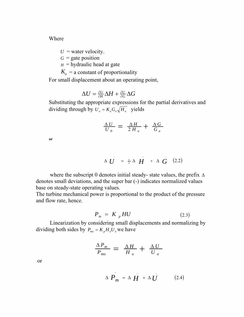
Where U = water velocity. G = gate position H = hydraulic head at gate uK = a constant of proportionality For small displacement about an operating point, GHU G

UHU ∆+∆=∆ ∂

∂∂∂

Substituting the appropriate expressions for the partial derivatives and dividing through by oouo HGKU = yields

oo GG

HH

UU ∆∆∆ += 20

or

GHU−−−

∆+∆=∆ 21 ( )2.2

where the subscript 0 denotes initial steady- state values, the prefix ∆ denotes small deviations, and the super bar (-) indicates normalized values base on steady-state operating values. The turbine mechanical power is proportional to the product of the pressure and flow rate, hence. HUKP pm = ( )3.2 Linearization by considering small displacements and normalizing by dividing both sides by oopmo UHKP = we have

oomo

mU

UH

HP

P ∆∆∆ += or

UHPm−−−

∆+∆=∆ ( )4.2

Substituting for U−

∆ from equation (2.2) yields

GHPm−−−

∆+∆∆ = 5.1 ( )a5.2 Alternatively, by substituting for H∆ from equation (2.2) we may write GUmP

−−

∆∆=∆ − 23 ( )b5.2

The acceleration of water column due to the change in the head at the turbine, characterized by Newton’s second low of motion, may be expressed

as ( ) HaALA gdt

Ud ∆−=∆ ρρ )( ( )6.2 where lengthL = of conduit =A pipe area mass=ρ density onacceleratiag = due to gravity massLA =ρ of water in the conduit lincrimentaHag =∆ρ change in pressure at turbine gate timet = in seconds By dividing both sides by oog UHaAρ the acceleration equation in normalized form becomes

( )ooog

oH

HU

Udtd

HaLU ∆∆ −=

or

−−

∆−=∆ Hdt

UdT w ( )7.2

Where by definition,

0

0

HaLUT

gw = ( )8.2

Here wT is referred to as the water starting time. It represents the time required for the head oH to accelerate the water in the penstock from standstill to velocity oU . It should be noted that wT varies with load. Typically wT at full load lies between 0.5 s and 4.0 s. Equation ( )7.2 represents an important characteristic of the hydraulic plant. A descriptive explanation of the equation is that if the back pressure is applied at the end of the penstock by closing the gate, then the water in the penstock will decelerate. That is if there is positive pressure change, there will be negative acceleration change. From equation ( )2.2 and ( )7.2 we can express the relationship between change in velocity and change in gate position as

⎟⎠⎞

⎜⎝⎛ ∆−∆=

−−∆

−

UGdtd

wUT 2 ( )9.2

Replacing dtd with the Laplace operator s, we may write

⎟⎠⎞

⎜⎝⎛ ∆−∆=

−−−∆ UGUsT w 2

Or

−

+

−

∆=∆ GU sT w)(11

21 ( )10.2

Substituting for U−

∆ from equation ( )B5.2 and rearranging, we obtain

sT

sTm

w

w

G

P

211

1

+

−−

−

=∆

∆ ( )11.2

2.4 Governors for hydraulic turbines: The function of a governor is to control speed and/or load. The primary speed/load control function involves feeding back speed error to control the position. In order to ensure satisfactory and stable parallel operation of multiple units, the speed governor is provided with a droop characteristic. The steady state droop is set at about 5% such that a speed deviation of 5% causes 100% change in gate position or power out put, this corresponds to a gain of 20.For hydro turbine, such a governor with a simple Steady state characteristic would be unsatisfactory. This can explained by the following simple calculation using a simplified block diagram representation of speed control of hydraulic generating unit feeding an isolated load is shown in figure E2.2 the turbine is represented by the classical model and speed governor by pure gain.

RKg

1= . The generator is represented in terms of combined inertia of the

generator and turbine rotors. If sTw 0.2= , sTm 0.10= , and 0.0=DK ,determine (i) the value for the droop R for which the speed governing is stable, and (ii) the value of R for which the speed control action is critically damped. Solution The characteristic equation (of the form 1+GH=0) of the closed -loop system is 01 1

101

121 =+ +

−Rss

s Or ( ) 0121010 2 =+−+ sRRs

Fig 2.2 block diagram of speed control of hydraulic generating unit

(i) For stability, the roots of the characteristic equation have to be in the left side of complex s-plane. In case of a quadratic, a sufficient and necessary condition is that all quadratic coefficients are positive. Hence,

010 ⟩R , i.e., 0⟩R And 0210 ⟩−R , i.e., 2.0⟩R The smallest value of R resulting in stable response is thus 0.2 or

20%. In other words, the speed governor gain Gk has to be less than 5. With the standard 5% droop (or gain of 20) the speed control would be unstable.

(ii) For critical damping

( ) ( ) 0104210 2 =−− RR Solving yields

746.01 =R 0536.02 =R With 746.01 =R corresponding to the critical damping (damping ratio 1=ζ ) represents stable response. And 0536.02 =R is less than the limiting value of 0.2; it corresponds to 0.1−=ζ and represents unstable operation. Therefore, 746.0=R or gain 34.1=GK is required for critical damping.

2.5 Requirement for a transient droop A change in gate position produces an initial turbine power change which is opposite to that sought. For stable control performance, a large transient (temporary) droop with along resetting time is required. This accomplished by the provision of a rate feed back or transient gain reduction. The rate feedback retards or limits the gate movement until the

water flow and power output has time to catch up. The result is a governor, which exhibits a high droop (low gain) for fast speed deviations, and the normal low droop (high gain) in the steady state

2.6 Electro hydraulic governor Modern speed governors for hydraulic turbines use electro hydraulic systems. Functionally, their operation is very similar to that of mechanical-hydraulic governors. Speed sensing, permanent droop, temporary droop, and other measuring and computing functions are performed electrically. The components provide greater flexibility and improved performance with regard to deal with bands and time lags. The dynamic characteristics of electric governors are usually adjusted to be essentially similar to those of mechanical-hydraulic governors 2.7 Tuning of speed governing systems 1- Stable operation during system-islanding conditions or isolate operation 2- Acceptable speed of response for loading and unloading under normal synchronous operation. For stable operation under isolating conditions, the optimum choice of the temporary droop TR and reset time RT is related to the water starting time WT and mechanical starting time HTM 2= (see chapter 3, section 3.9.3 of Power System Stability And Control) as follows [14]:

( )[ ]M

WTT

WT TR 15.00.13.2 −−= ( )[ ] WWR TTT 5.00.10.5 −−= In addition the servo system gain SK should be set as high as is practically possible. The above setting ensures good stable performance when the unit is at full load supplying an isolated load. This represents the most severe requirement and ensures stable operation for all situations involving system islanding. For loading and unloading during normal interconnected system operation, the above settings results in too slow response. For satisfactory loading rates, the reset time RT should be less than 1.0 s preferably close to 0.5 s.

The above conflicting requirements may be met by using the dashpot bypass arrangement as follows: With the dashpot not bypassed, the settings satisfy the requirements for system-islanding conditions or isolated operation. With the dashpot bypassed, the reset time RT has a reduced value, resulting in acceptable loading rates. The dashpot is normally not bypassed, so that in the event of a disturbance leading to an islanding operation, speed control would be stable. The dashpot is bypassed for brief periods during loading and unloading. 2.8 PID governor Some electro hydraulic governors are provided with three-term controllers with proportional-integral-derivative PID action. These allow the possibility of higher response speeds by providing both transient gain reduction and transient gain increase. The derivative action is beneficial for isolated operation, particularly for plants with water starting time sTW 3= or more. Typical values are 0.3=PK 7.0=IK , and 5.0=DK . However the use of high derivative gain or transient gain increase will result in excessive oscillations and possibly instability when the generating unit is strongly connected to an interconnected system. Therefore the derivative gain is usually set to zero; without the derivative action, the transfer function of a PID now PI governor is equivalent to that mechanical-hydraulic governor. The proportional and integral gains may be selected to result in the desired temporary droop and reset time. 2.9 Guidelines for Modeling Hydraulic Turbines The modeling detail required for any given study depends on the scope of study and system characteristics. The following are the guidelines: 2.9.1 Governor tuning studies Significant differences exist between frequency response characteristics of the exact elastic model and simplified inelastic model of the water column, beyond 0.1 Hz. These differences have negligible effect on conventional governor with transient droop compensation or equivalent PI controller. The larger band width of PID controllers requires a more accurate representation of the penstock water column. Usually a lumped parameter approximation would be acceptable. The surge tank natural period is on the order of several minutes. Its representation in governor tuning studies is usually not necessary.

2.9.2 Transient Stability Studies The hydraulic turbine governors have a very slow response from the viewpoint of transient stability. Their effects are likely to be more significant in studies of small isolated systems. A nonlinear turbine model assuming inelastic water column would adequate for such studies. The speed governor model should account gate position and rate limits. 2.9.3 Small-signal Stability Studies The speed governors have negligible effect on local plant mode oscillations of frequencies of the order of 1.0 Hz. However, the effect on low frequency interarea oscillations of frequency below 0.5 Hz may be significant. These effects can be modeled adequately by linearizing the nonlinear turbine-penstock. For plants with long penstocks; it may be prudent to consider the water hammer effects. Small signal studies are also ideally suited for investigating interactions between the hydraulic system dynamics and the network power oscillations. 2.9.4 Long Term Dynamic Studies Depending on the nature of the problem, a very detailed nonlinear representation of the turbine and water column dynamics may be required. This includes traveling wave effects and tank dynamics. Such studies are invaluable for studying problems associated with special plant layouts and establishing appropriate operating procedures. 2.10 Excitation systems: The basic function of an excitation system is to provide direct current to the synchronous machine field winding. In addition the excitation system performs control and protective functions essential to the satisfactory performance of the power system by controlling the field voltage and thereby field current. The control includes: 1\ Control of voltage 2\ Control of reactive power flow 3\ Enhancement of system stability The protective functions ensure that the capability limits of synchronous machine, excitation system, and other equipment are not exceeded. 2.10.1 Generator considerations The basic requirement is that the excitation system supplies and automatically adjusts the field current of synchronous generator to maintain the terminal voltage as the output varies within the continuous capability of the generator. Normally the exciter rating varies from 2.0 to 3.5 MVA

KW of generator rating.

In addition the excitation system must be able to respond to transient disturbances with field forcing consistent with the generator instantaneous and short- term capabilities. The generator capabilities are limited by: 1\ Rotor insulation failure due to high field voltage. 2\ Rotor heating due to high field current. 3\ Stator heating due to high armature current loading 4\ Core end heating (during under excited operation) 5\ Heating due to excess flux volt/Hz. The thermal limits have time dependent characteristics; the short term over load capability of the generator may extend from 15 to 60 seconds. 2.10.2 Power System Considerations The excitation system should contribute to effective control of voltage and enhancement of system stability. It should be capable of responding rapidly to a disturbance so as to enhance transient stability, and of modulating the generator field so as to enhance small signal stability. Using auxiliary stabilizing signal, in addition to terminal voltage error signal, to control the field voltage to damp system oscillations, expanded the role of the excitation system. This of excitation control is referred to as power system stabilizer. 2.10.3 Power System Stabilizer PSS The power system stabilizer uses auxiliary stabilizing signals to control the excitation system so as to improve power system dynamics performance. Input signals to PSS are shaft speed, terminal frequency and power. Power system dynamic performance is improved by the damping of system oscillations. This is a very effective method of enhancing small-signal stability performance. The basic function of power system stabilizer PSS is to add damping to the generator rotor oscillations by controlling its excitation using auxiliary stabilizing signals. To provide damping, the stabilizer must produce a component of electrical torque in phase with the rotor speed deviations.

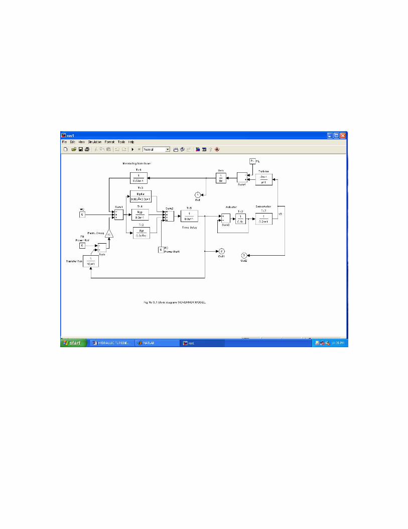
Chapter (3) Simulation of dynamic models 3.0 Introduction: The dynamic model used to simulate the power unit of the hydro power station at ROSEEIRES is built using SIMULINK control blocks. The machine blocks describing the complete unit are Governor model. Generator model A.V.R. model A.V.R. and generator model. SIMULINK 3.1 Governor model: Fig No 3.1Governor block diagram

The hydro generator of ROSEIRES hydropower station is depending strongly on turbine governor system to be stable, and stabilizes the grid. The governor turbine model is shown in Fig 3.1. The main controller used for transient gain control is PID controller which has proportional, integral and derivative control components. The permanent droop is represented by the gain K. Servomotor and Actuator time lags are set by ( )7Tr and ( )6Tr . The turbine is modeled using the classical turbine model with water starting time of 2 seconds.

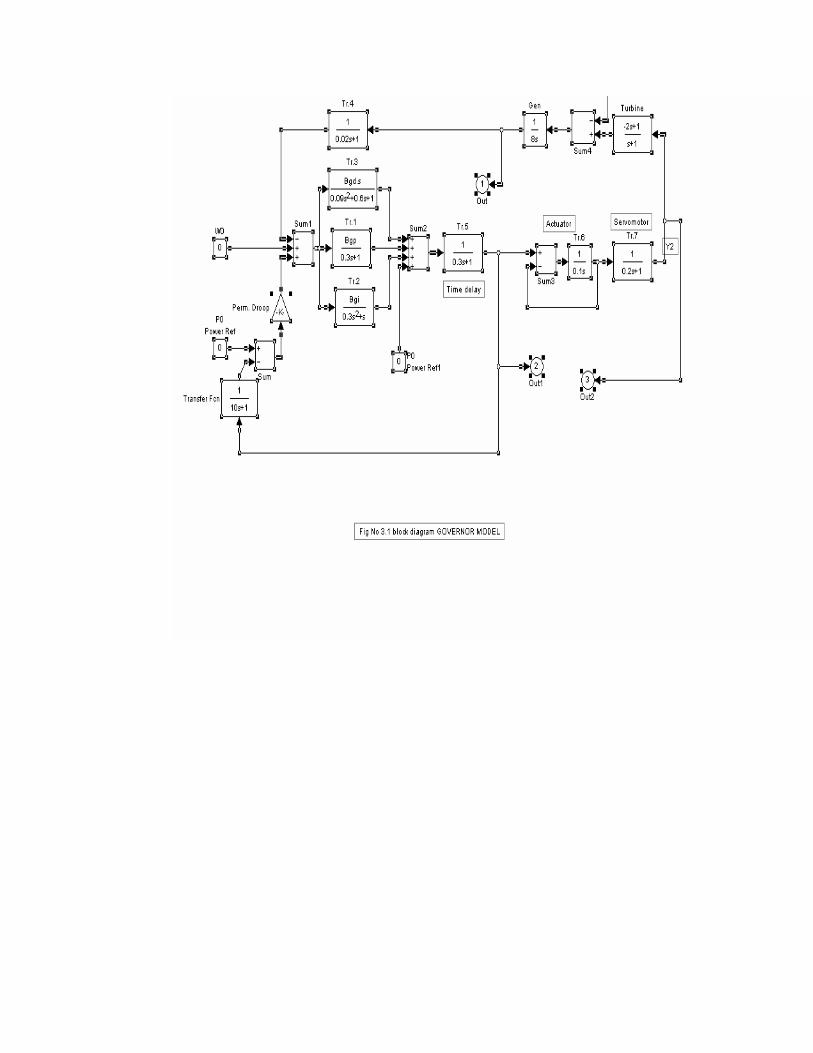
Other components are measuring transducer equivalent circuit ( )4Tr and time delay ( )5Tr . ( )0w and ( )0P are the speed and power references. Various outputs describing the speed and gate signals are taken from nodes 1, 2 and 3.

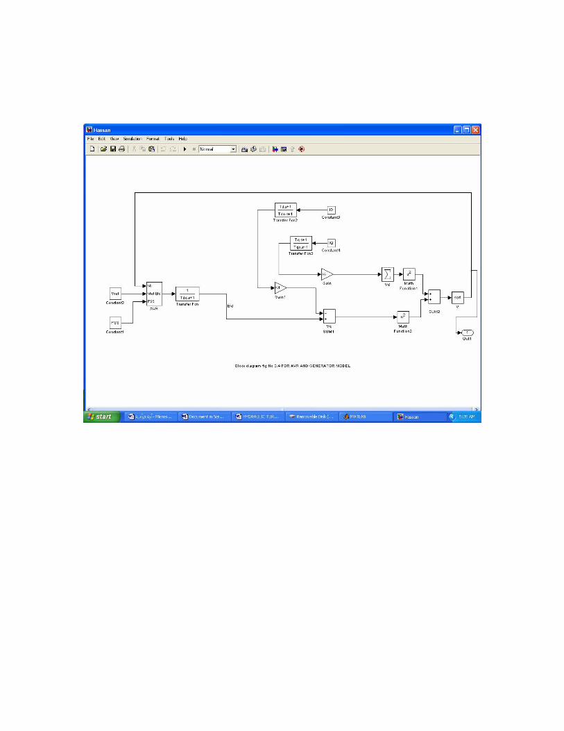
3.2 Generator model: Fig No 3.2 Generator block diagram The generator model used provides change in flux linkages on both the d-axis and the q-axis, the flux delay components on both axes are presented by time constants ( )0Td , ( )Td , ( )Tq and ( )0Tq . Inputs to the model are provided by ID and IQ which are MATLAB functions coded for computation of d-axis and q-axis currents. The field voltage ( )Efd is obtained from the output of the exciter model. The flux linkage voltage ( )Vd and ( )Vq are vectorially summed using ( )2U and square root function to yield terminal voltage ( )V . Note Leakage flux is neglected 3.3 Automatic voltage regulator model: Fig No 3.3 A.V.R. block diagram The basic control functions of the A.V.R. are the following

• Voltage regulator with PID filter • Reactive and active current compensation • Power factor / reactive current regulation • Smooth distribution of reactive power between parallel

machines • Limiters for

1- Maximum and minimum field current 2- Maximum stator current lead/lag 3- Under excitation 4- Volts-per-Hertz

• Power system stabilizer ( )cV from machine terminal component controlled by ( )refV , all together with the component of active and reactive power P,Q, are influenced by time constant ( )ai TT , , and different limiters are to produce ( )fdE . 3.4 Automatic voltage regulator and the generator:

Fig No 3.4 A.V.R. plus generator block diagram The A.V.R and the generator models are combined into one equivalent model shown in Fig 3.3 The A.V.R is set up of ( )fdE component, processed through the time constant ( )0dT and the generator components. Within the other part of the model, the flux linkage of ( )qd , axes are

presented by time constants dT , doT and qT , qoT .

The flux linkage voltages dV and qV are summed using 2U and root squared to get ( )V which is the machine terminal voltage

3.5 Matlab: MATLAB, developed by math works Inc., is software package for high performance numerical computation visualization. The combination of analysis capabilities, flexibility, and powerful graphics makes MATLAB the premier software package for electrical engineers. MATLAB provides an interactive environment with hundreds of reliable and accurate build-in mathematical functions. These functions provide solutions to a broad range of mathematical problems including matrix algebra, complex arithmetic, linear system, differential equations, signal processing, optimization, nonlinear systems, and many other types of scientific computations. The most important feature of MATLAB is its programming capability, which is very easy to learn and to use, which allows the user developed functions. It also allows access to FORTRAN algorithms and C codes by means of external interfaces. There are several toolboxes written for special applications such as signal processing, control system design, system identification, statistics, neutral networks fussy logic, symbolic computations, and others. MATLAB has been enhanced by the very powerful SIMULINK program. SIMULINK is a graphical mouse-driven program for the simulation of dynamic systems. SIMULINK enable the students to simulate linear, as well as nonlinear, systems easily and efficiently. 3.6 Simulink: 3.6.1 Simulink is an interactive environment for modeling, and simulating a wide variety of dynamic system. SIMULINK provides user interface for constructing block diagram models using “drag-and-drop” operations. A system is configured in terms of block diagram representation from a library of standard components. SIMULINK is very easy to learn. A system in block diagram representation is built easily and the simulation results are displayed quickly. Simulation algorithms and parameters can be changed in the middle of a simulation with intuitive results, thus providing the user with access learning tool for simulating many of the operational problems found in the real world. SIMULINK is particularly useful for studying the effects of nonlinearities on the behavior of the system, and as such, it is an ideal research tool. 3.6.2 Simulation parameters and solver

You set the simulation parameters and select the solver by choosing parameters from the simulation menu. SIMULINK displays the parameters dialog box, which uses three “pages” to manage simulation parameters. Solver, Workspace I/O, and Diagnostics. 3.6.3 Workspace Input-Output page The Workspace I/O page manages the input from and the output to the MATLAB workspace, and allows:

• Loading input from the workspace – Input can be specified either as MATLAB command or as a matrix for the import blocks.

• Saving the output to the workspace –You can specify return variables by selecting the time, State, and/or output check boxes in the Save to workspace area.

3.6.4 Block diagram construction At the MATLAB prompt, type SIMULINK. The SIMULINK BLOCK LIBRARY, containing seven icons, and five pull-down menu heads, appears. Each icon contains various components in the title category. To see the content of each category, double click on its icon. The easy-to-use pull-down menus allow you to create a SIMULINK block diagram, or open an existing file, perform the simulation, and make any modifications. Basically, one has to specify the model of the system (state space, discrete, transfer function, nonlinear ode’s, etc), the input (source) to the system, and where the output (sink) of the simulation of the system will go. Generally when building a model, design it first on the paper, then build it using the computer. When you start putting the blocks together into a model, add the blocks to the model window before adding the lines that connect them. This way you can reduce how often you need to open block libraries. An introduction to SIMULINK is presented by constructing the SIMULIK diagram for the following examples. 3.6.5 Modeling equation Here are some examples may improve understanding: Model the equation that converts Celsius temperature to Fahrenheit. TF = 9/5TC + 32 Consider the blocks needed to build the model. These are:

• A ramp block to input the temperature signal, from the source library.

• A constant block, to define the constant of 32, also from the source library.

• A gain block, to multiply the input signal by 9/5, from the linear library.

• A sum block, to add the two quantities, also from linear library.

• A scope block to display the output, from the sink library. To create a SIMULINK block diagram presentation select new… from the File menu. This provides an untitled blank window for dressing and simulating a dynamic system. Copy the above block from the block libraries into the new window by depressing the mouse button and dragging. Assign the parameter values to the Gain and Constant blocks by opening (double click) on each block and entering the appropriate value. Then click on the close button to apply the value and close the dialog box. The next step is to connect these icons using the left mouse button (hold the button down and drag the mouse to draw a line). Now you have the SIMULINK block diagram.

Chapter (4) Optimization of (PID) controller parameters for machine at ROSEIRES Introduction: Through this chapter, one shall investigate optimum settings for the PID controller for machines at ROSEIRES hydropower station. The machine operating mode has three distinct differences 4. i Machine operating at no load PL=0

4. ii Machine operating in an isolated mode (Island Operation) 4. iii Machine operating in an interconnected mode.

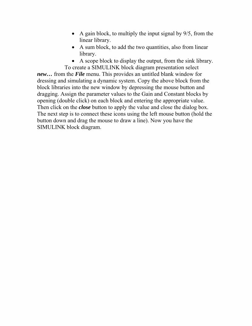
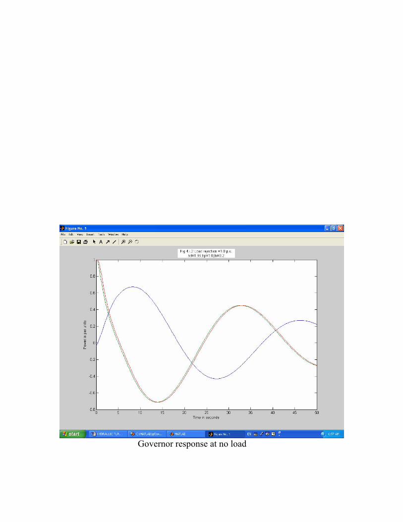
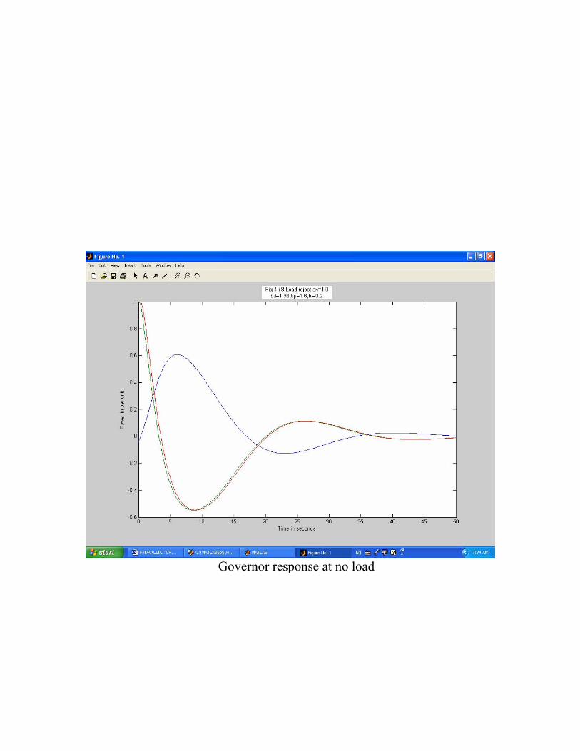
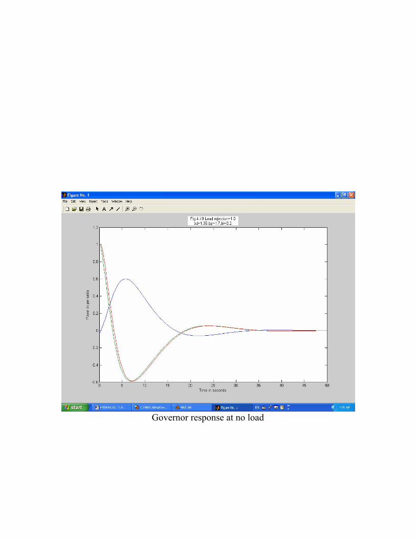
It is generally reported in the literature that the normal mode, when the station is in an interconnected mode requires only proportional and integral control bi and bp, while derivative control (bd) is added under conditions of islanding, Island operation. The determination of correct settings from the design point of view is an entirely complicated task and additionally does not cater for non linearity. Thus, one of the reliable methods is to resort to straightforward SIMULATION of the system operation. 4. i No load operation mode: In this mode of operation, the units at ROSEIRES were tested for a complete load rejection of 1 per unit i.e. 40 MW per machine. The program implementing this test is shown in Appendix 1.0 The proportional, integral and derivative components appear to have a certain behavior towards no load operation mode. A MATLAB program for simulating the governor is set to run different settings and adjustments of the PID components, with results of unstable operation. Finally steady state condition reached out at settings of PID as 96.1=db

8.1=pb

2.0=ib On the following pages are plotting for every setting of the PID controller within the no load operation.

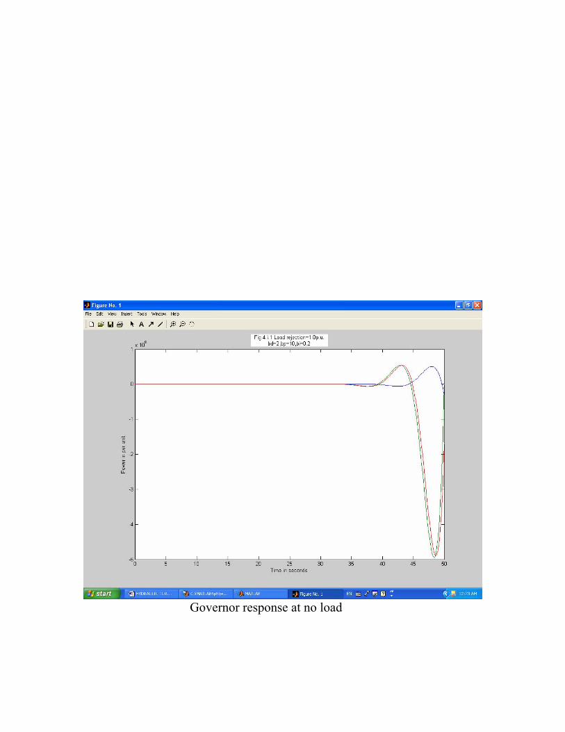
Governor response at no load

Governor response at no load

Governor response at no load

Governor response at no load

Governor response at no load

Governor response at no load

Governor response at no load

Governor response at no load

Governor response at no load

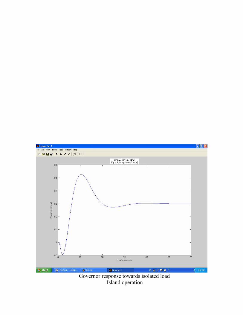
4. ii Operation in isolated mode (Island operation): In this case the machines are not connected to the external network. One machine is simulated and a 30% equivalent to about 12MW step load is applied to the terminals of the machines. The SIMULATION starts with derivative control off 0=db and oscillations are improved by gradually adding the derivative components A group of plots showing the convergence to optimum performance with the fastest setting time and maximum damping are presented below. The program studying this case is configured in Appendix 2.0

Governor response towards isolated load Island operation

Governor response towards isolated load Island operation

Governor response towards isolated load Island operation

Governor response towards isolated load Island operation

Governor response towards isolated load Island operation

Governor response towards isolated load Island operation

Governor response towards isolated load Island operation

Governor response towards isolated load Island operation

Governor response towards isolated load Island operation

As one may observe from plots, oscillations damping improves when adding a derivative component. If one starts with 0=db , then continue on increasing the parameter up, the best response is obtained with 2.0=ib and 8.1=pb The oscillations have a period of about 0.07 Hz and damping is poor see Figure 4.ii.1. Adding db in steps of 0.5 shows improved damping up to

5.2=db see Figure 4.ii.2 ……up to Figure 4.ii.5

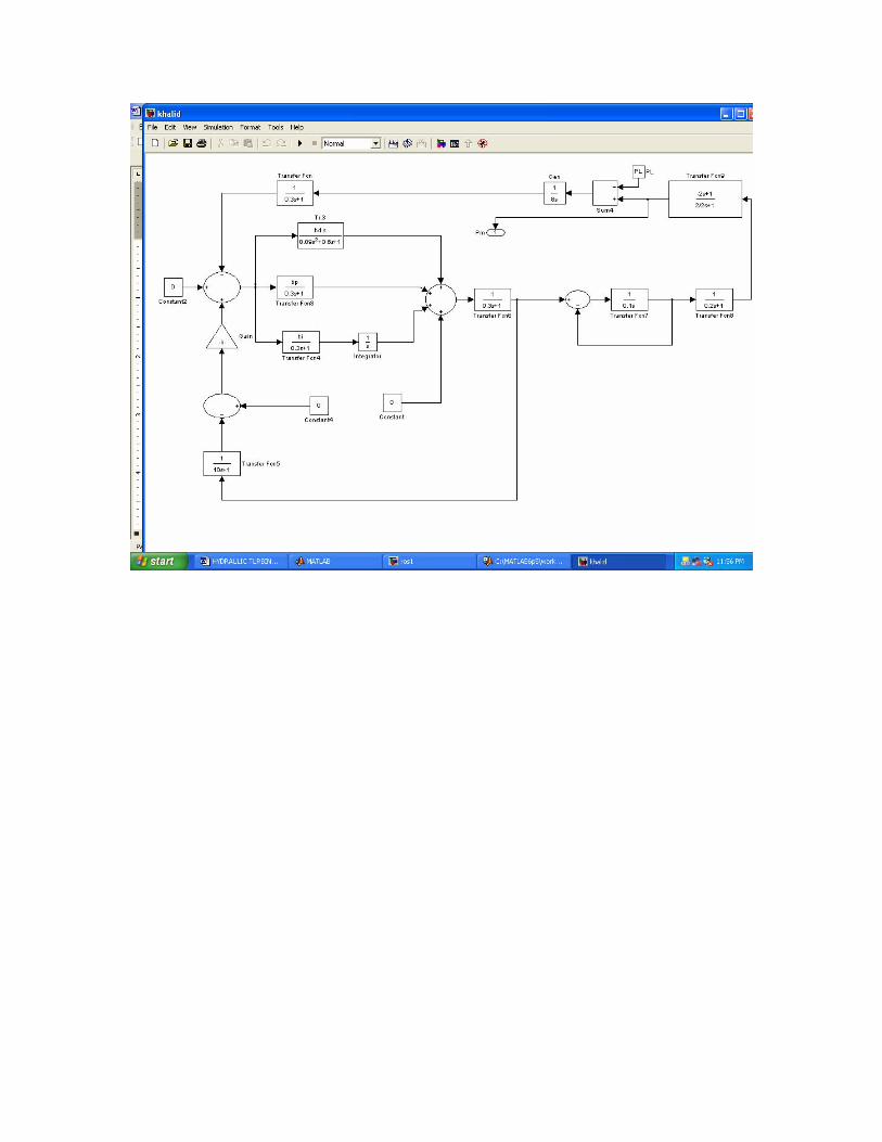
Increasing db further drives the system into amplified initial oscillations, although the system settles down subsequently see Figure 4.ii.7 ……up to Figure 4.ii.9. We may conclude thus that the best response is achieved by setting 2.0=ib , 8.1=pb and 5.2=db 4. iii Optimum(PID)parameters for machines at ROSEIRES for interconnected operation: In the optimization of PID parameters we started with machine operating in isolated island mode, but now the study changes to suit machine operating in interconnected mode. As mentioned before, the literature describes the operation of machines in an interconnected mode as relaying only on an integral and proportional control ( )ip bandb , , while db is usually set to zero. For this mode of operation, a new model was developed and programmed using SIMULINK and MATLAB, which simulates the operation of the machines at ROSEIRES hydro power station. The machines are interconnected to the rest of the system, modeled by an infinite bus bar of °∠01 voltage, over along transmission line. See appendix 3.0 for program code.

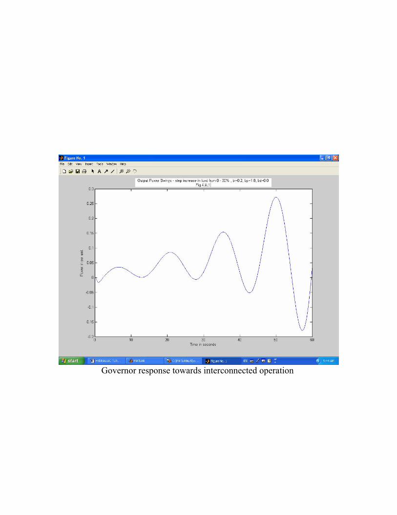
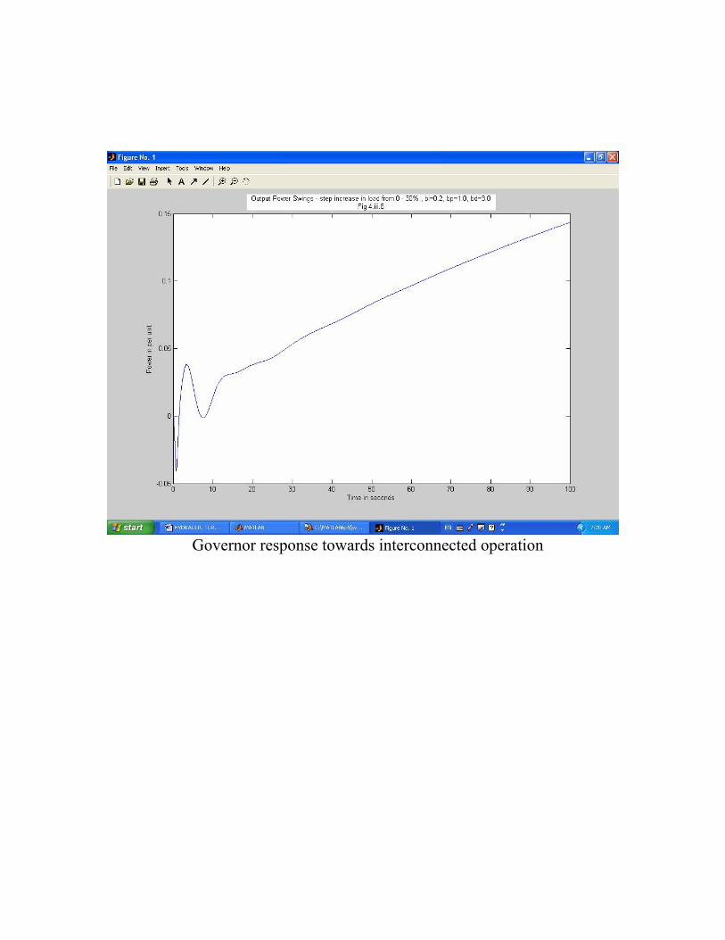
4. iii Operation in interconnected mode: The machine at this stage is connected to the network; and a 30% step increase in the machine power is applied to the machine terminals. The SIMULATION starts with

0=db

8.1=pb

2.0=ib The unstable and oscillating condition is clearly observed, which improved by gentle varying ( )ip bb , until stable operating condition is reached. Various plotting are presented below so that the optimum performance will be shown.

Governor response towards interconnected operation

Governor response towards interconnection operation

Governor response towards interconnected operation

Governor response towards interconnected operation

Governor response towards interconnected operation

Governor response towards interconnected operation

Governor response towards interconnected operation

Governor response towards interconnected operation

As the plots show it was found necessary to reduce both values of ib and pb from 0.2 and 1.8, respectively to 0.1 and 1.0

It was found also necessary to add a derivative term 0.3=db At these settings the oscillations die out quickly and the machines output travels very slowly towards the set point of 30% 0.3 per unit. The difference from the expected output is that a derivative term was found necessary in this case, while most sources and texts mentioned that it is usually set to zero for interconnected operations. This may be explained by noting that ROSEIRES hydro power station is weakly coupled to the remainder of the system, over 500 Km 220 Kv transmission line a single conductor connection.

Chapter (5) Comparison between findings and existing PID controller settings The machines at ROSEIRES at present are undergoing extensive overhauling for governing system under station automation project. All settings are expected to be retuned. However the existing setting on the governors may serve as an indication to proper operation of the station, even though these settings may not be optimum. For example, the settings found on unit number 6 were as follows

(i) Island operation mode 2.4=pb

5.0=ib 0.3=db

(ii) Interconnected operation mode 2.6=pb

7.3=ib 9.2=db

We note that the settings differs from what was found by simulation and presented in Chapter (4) which are as follows

(i) Island operation mode

8.1=pb

2.0=ib

5.2=db (ii) Interconnected operation mode

0.1=pb

1.0=ib

0.3=db It was well known that the old settings caused problems in the operation, hunting of the machines, resulting in an undesirable frequency oscillations within the system, mechanical wear out for the wicket gates and servo motors which is one of the main causes for life time reduction, in particular during black start operation when the hydro station is required to start energizing the grid following a black out occurrence. It was observed that when any of the machines was synchronized and the loading increased, oscillations start to build up and become sustained. The frequency may go up to values that causes the over frequency protection to trip the unit 52 Hz or may go down to values which operate the low frequency load shedding schemes on some of the feeders. As an example, Figure 5.1 shows an attempt to start machine number 7, following the system black out at 9Hrs23 am on 19 october2003. The plots were obtained from the fault recorder, slow records, at ROSEIRES substation. The plots shows quite clearly that the machine starts and continue stable on bars with minimum hunting at first, but as the load increases it suddenly bursts into severe oscillations until it trips over. It is a clear indication that the setup of the PID controller on that machines is very far from optimum.

Chapter (6) Conclusion and Recommendations The PID controllers of the hydro machines, in ROSEIRES play a major role in the system oscillations and stabilize the network. The study shows clearly that the key to a successful implementation of the PID controller is the correct tuning of the parameters. Furthermore it proves that the set of parameters for no load operation is different from those for island and interconnected operations. When comparing the study results with the old settings the values

were found to differ, especially for the integral component ( )ib . Thus that may explain some of the observed instability of the system in reality.

It was generally observed that a reduction in both ( )ib and ( )pb was necessary to enhance stability. The study also shows that the nature and period of oscillations 0.07-----0.08Hz is similar to the observed oscillations on the hydro machines, from the fault recorder data. These modes of operation are typical of the hydro machines and in the absence of a powerful controller such as PID control or transient gain reduction control would make the operation of the hydro units possible only at extremely reduced gains. It is recommended to put the new settings into practice whenever possible and whenever applicable for the hydro machine at ROSEIRES. It is further recommended to execute the already planned third circuit, would be expected to strengthen the coupling between the hydro station and the remainder of the grid, resulting in better performance. It is also necessary carry out similar studies to this work whenever a new governor is installed in any of the hydro generators. The basic fact to emphasis here is that the governor of the hydro station need special attention, and must contain a properly tuned PID controller. They cannot and must not be treated as ordinary control devices which contain only conventional PI controllers.

REFERENCES

REFERENCES

• Power System Stability And Control P. KUNDUR • Mastering MATLAB

DUANE HANSELMAN • ASEA Manuals • ABB Manuals • VA TECH VOEST MCE Basic Hydraulic Layout of Turbines

APPENDICES

APPENDIX (1)

• MATLAB program to study units at ROSEIRES under no load operation. • ROSEIRES hydro power station original Governor diagram.

APPENDIX (2)

• MATLAB program to test the units at ROSEIRES under island operation mode.

• Governor system case (1) diagram • A.V.R. and Generator diagram • MATLAB user functions to compute direct axis (Id) and

quadrate axis (Iq) currents.

APPENDIX (3)

• MATLAB program to study units at ROSEIRES under interconnected system conditions

• A.V.R. and Generator diagram • Governor system case (1) diagram • Governor system case (2) diagram • MATLAB program for computing direct axis (Id2) and quadrate axis (Iq2)