UNIVERSITY OF KHARTOUM - COREUNIVERSITY OF KHARTOUM FACULTY OF ENGINEERING & ARCHITECTURE DEPARTMENT...

1

بسم اهللا الرمحن الرحيم

UNIVERSITY OF KHARTOUM

FACULTY OF ENGINEERING & ARCHITECTURE

DEPARTMENT OF CHEMICAL ENGINEERING

STUDY OF HYDRODYNAMICS AND MASS TRANSFER OF OIL EMULSION IN A PILOT SCALE SIEVE TRAY COLUMN

A Thesis Submitted in Fulfillment Of the Requirements

For the Degree Of Ph.D in Chemical Engineering

Presented By Osman Tageldin Osman Supervised By Dr. Gurashi Abdalla Gasmelseed

Late : Dr. Osama Abdelhameed Abdalla

August 2005

2

Dedication

To the soul of great father

To my mother, wife and sons

With love

3

Acknowledgements

I would like to express my thanks to my late supervisor

,Dr.Osama.Adbdelhameed Abdalla for his unlimited help,

guidance, constant indispensable encouragement and invaluable

comments during the preparation of this thesis.

Also I would like to express my gratitude to Dr.Gurashi

Abdalla Gasmelseed for supervision and help in this thesis.

My thanks are also due to the staff of the chemical engineering

department and the Unit Operation Laboratory staff in the

University of Khartoum.

4

Abstract

A study of primary and secondary treated liquid petroleum wastes in a

pilot sieve tray column has been undertaken. The literature related to this

type of extractor and the relevant phenomena of droplet break-up and

coalescence, drop size and drop mass transfer have been reviewed.

The method of treatment in local refineries has been investigated and

it is observed that the primary and secondary processes are quite efficient,

but the tertiary process leaves some of the oil in he effluent and this is why

the treated water is not recycled and reused. The treated waste/oil water is

pumped into ponds for evaporation leaving the oil and other less volatile

components as a residue which have a negative impact on the environment.

The system of oil in water is not a normal solute-solvent system, and

to make it so the mixture has been emulsified with a surfactant producing a

partially water miscible emulsion. Experiments were carried out with non-

mass transfer to determine the operating column hydrodynamics such as

flooding. At 85% of flooding, mass transfer experiments were performed

and the effects of drop size, drop size distribution and dispersed phase

holdup volume at variable agitation speeds on the column performance

have been investigated.

The concentration profile has been measured and the overall

experimental mass transfer coefficients were calculated from the mean

driving force using Simpson's rule. It is observed that drop size, drop size

distribution and mass transfer coefficients were strongly dependent on the

speed of agitation. As the oil droplets were composed of emulsified oil in

water and the oil itself is completely immiscible in water, the direction of

mass transfer was from the emulsified droplets to the dispersed phase. This

condition coupled with high solubility of oil in n-hexane made the

extraction process very efficient and an almost oil-free water could be

obtained and recycled.

5

This work is also mainly intended to compare the experimental mass

transfer coefficients with those predicted by the models formulated by

Angelo et al and Rose et al. It is found that the data fitted very well when

correlated by the model formulated by Angelo et al, therefore it is

recommended for mass transfer prediction in agitated columns such as

sieve trays.

6

ملخص البحث

أجريت هذه الدراسة على مخلفات البترول الخام السائلة بعد معالجتها األولية والثانوية في

الخاصة بهذا النوع من المستخلص ، والظاهرة عالجة الم دراسة تتموقد . المناخلبرج صواني

.القطرات تكسر واندماج ون تكوالمتناسبة من

األولية والثانوية تتمـان ينالعمليتأن مصافي المحلية في ال الجةعم طريقة ال من لوحظوقد

لذا فأن المياه المعالجة ال يعـاد . بكفاءة عالية ، لكن العملية الثالثة تترك بعض الزيت في الدفق

وتضخ إلى البرك لكي تتبخر تاركـة الزيـت والمكونـات الغيـر . دورانها وإعادة استخدامها

كأنظمـة لـيس إن نظام الزيت فـي المـاء . على البيئة سالباً متطايرة كبقايا ، مما يترك أثراً

ولجعله كذلك فقد استحلب الخليط بعامل سطحي ينتج مستحلب مـائي قابـل ص العادية االستخال

وعنـد لطفحامثل لالمتزاج جزئياً ، وقد أجريت تجارب لتحديد التشغيل الهايدروديناميكي للبرج

القطرة ومرحلة مقاسانت أثار حجم القطرة وتوزيع ، أجريت تجارب وك لطفحمن ا % 85نسبة

.التشتت كلها تحرز سرعات هيجان متباينة على أداء البرج الذي تمت دراسته

التجريبية من متوسـط القـوة انتقال المادة وقد تم قياس التركيز كما تم حساب معامالت

حجـم القطـرة ومعامـل وقد لوحظ إن حجم القطرة وتوزيع . الدافعة باستخدام قاعدة سيمسون

قطرات الزيت قد تكونـت مـن زيـت نوبما إ . كانت تعتمد على سرعة الهيجان المادةتحول

مستحلب في الماء وكان الزيت نفسه غير مذاب كامالً في الماء فأن اتجاه نقل الكتلة كان كبيـراً

للزيت في العالية جداً من القطرات المستحلبة في مرحلة التشتت ، وهذه الحالة مصحوبة باإلذابة

مادة الهكسين جعلت عملية االستخالص ذات كفاءة عالية وبذا يمكن الحصول على ماء خالي من

. دورانهإعادةالزيت و

معامالت انتقال المادة بحيث أن النموذج الذي صممه أنجلو لحساب ج ذتم استخدام نما وقد

ذج الذي صممه أنجلو وآخرون وآخرون طبق وقورن مع نموذج روز وآخرون ، وتأكد أن النمو

وبناءاً على . نموذج روز وآخرون يعطي أقل انحراف من معامالت االنتقال التجريبية مقارنة مع

هذه النتيجة يوصي أن يستخدم نموذج أنجلو وآخرين في تحديد معامالت إنتقـال المـادة عنـد

. واألجهزة المماثلةالمناخل سائل في برج صواني -إستخالص سائل

7

List of Contents Content ………………………………………………..… PageDedication………………………...………………………………. i Acknowledgement………………………...……………………… ii Abstract………………………...…………………………………. iii Arabic Abstract………………...…………………………………. v List of Contents………………………...………………………… vi List of Tables …………...……………..………………………… viii List of Figures…………...………………………………………... x Nomenclatures…………………………………………………….. xi Chapter One……………………...……………………... 1.1 Introduction……………...…………………………………… 1 1.2 Stable Drop size……………...……………………………… 3 1.3 Drop Size Distribution in Agitated Systems……………........ 3 1.5 General objectives……………………………………….. 5 1.6 Specific objectives……...…………………………………….. 5 Chapter Two………………………...………………….. 6 2.1 Droplet Phenomena ……...………………… 6 2.2 Drop Formation:…………...……… 6 2.3 Droplet Break-up …………………………. 9 2.4 Droplet Coalescence...………. 10 2.4.1 Coalescence Fundamentals...…………………………... 11 2.4.2 Drop-Interface Mechanism ………………………. 11 2.4.3 Drop-drop coalescence Mechanism ……………………… 13 2.5 Drop Size Distribution ……………...…….... 15 2.6 Mass Transfer Fundamentals ….. 18 2.7 Mass Transfer During Drop Formation ………………… 19 2.8Mass Transfer During Drop Travel through the Continuous Phase ……………………………………….

21

2.9 Mass Transfer in the Dispersed Phase …… 22 2.9.1 Stagnant Droplets … 23 2.9.2 Circulating Droplets:………………….. 23 2.9.3 Oscillating Droplets:…….. 25 2.10 Mass Transfer in the Continuous Phase …………... 27 2.10.1 Mass transfer From and to Stagnant Droplets ……….. 28 2.10.2 Mass transfer From and to Circulating Droplets ……. 28 2.10.3 Mass transfer From and to Oscillating Droplets …… 31 2.11 Mass Transfer During Coalescence ……………. 31 2.12 Overall Mass Transfer Coefficients ……………… 33 2.13 Application of Single Drop Mass Transfer Models to Agitated Extraction Columns …………………………

33

8

2.14 Mass Transfer and Interfacial Instability ……………… 34 2.15 Effect of Surface Active Agent ……………...……… 36 2.16.1 Mass Transfer Models ………...………………………. 37 2.16.2 Stage Model……… 39 2.17. behaviour of drops in oil-water Emulsion ……………….. 41 2.17.1 Analysis of drop ……………...……………………. 42 2.17.2 Drop size measurement ………...…………………… 42 2.18 Equipment Classification……………...……………………. 42 2.19 Selection of Equipment……………...……………………… 43 2.20.1 Phase Equilibrium……………...………………………… 48 2.20.2 Tie-line Correlations……………...……………………… 49 2.20.3 Othmer and Tobias' Correlation……………...………… 50 2.20.4 Hand's Correlation……………...……………………….. 50 2.20.5 Ishida's correlation……………...……………………… 51 Chapter Three………………………...………………… 3.1 Selection of Liquid-Liquid Chemical Systems…………….... 52 3.2 Sampling Procedures ……………...…………………….. 52 3.3 Description of Equipment ………………….. 53 3.3.1 Determination of flooding points:……………...……… 54 3.4 Experimentation ……………...………………… 56 3.5 Determination of Equilibrium ……………………. 56 3.6Calculation Method …………...…………………………… 56 3.6.1 Experimental mass transfer coefficient ………...…….. 57 3.6.2 Theoretical mass Transfer Coefficient ……… 59 Chapter Four………………………...………………….. 4.1 Result ……………...…………………………………….. 62 4.2 Discussions ……………...………………………. 88 4.2.1 Column Hydrodynamics …………………………….. 89 4.2.2 Analysis of Results: 90 4.2.3 Experimental mass transfer coefficient 91 4.2.4 Theoretical mass transfer coefficient …….. 91 Chapter Five………………………...…………….. 100 CONCLUSION AND RECOMMENDATIONS 94 5.2 Recommendations.………………………… 95 References………………………...…………………….. 96 Appendixes………………………...…………………….. 100

9

List of Tables

Tables …………………………………………..……..… PageTable (2.1) Factors Affecting Coalescence Time 12 Table (2.2) Comparison between Normal and Log-Normal Distribution Dispersion……………………………………………

17

Table (2.3) : Correlation for Mass Transfer During Drop Formation ………………….

20

Table (2.4) Correlation for Continuous Phase Mass Transfer Coefficient ……………………………………………

30

Table (2.5) 5 Continuous Differential Contactors …………. 45 Table (2.6) Advantages and Disadvantages of Various Contractors 47 Table (4.1).Determination of flooding points at different speeds. 62 Table (4.2) Drop Sizes, number of drops and cumulative volume at 200 rpm. Without mass transfer………... ………………………

64

Table (4.3)Determination of Sauter mean diameter (d32),Agitator Speed 200 rpm. Without mass transfer………... ………………

65

Table (4.4) Drop Sizes, number of drops and cumulative volume at 300 rpm. Without mass transfer………... ………………………

66


67


68


69


70


71

Table (4.10) Drop Sizes, number of drops and cumulative volume at 200 rpm. With mass transfer. ………...……………………..

72

Table (4.11)Determination of Sauter mean diameter (d32),Agitator Speed 200 rpm. With mass transfer. ………...…………………

73


74

Table (4.13)Determination of Sauter mean diameter (d32),Agitator 300 Speed rpm. With mass transfer ……………………..

75


76

10

Table (4.15)Determination of Sauter mean diameter (d32),Agitator Speed 500 rpm. With mass transfer. ………...………………

77


78

Table (4.17)Determination of Sauter mean diameter (d32),Agitator Speed 600 rpm. With mass transfer. ………...…………………

79

Table (4.18) Mass Transfer Results……………………….… 80

Table (4.19)Result of Calculation of V0 and ds and d0………….. 81 Table (4.20)Circulating drop mass transfer coefficient……... 82 Table (4.21)Comparison between mass transfer coefficient With calculated for different models…………………………..

83

Table (4.22) Comparison between mass transfer coefficient with different operating conditions…………………………………..

84

Table (4.23)Experimental and theoretical overall mass transfer coefficients…………………………………………………...

85

Table (4.24)Comparison between experimental and theoretical mass Transfer coefficients ratio…………………………………

86

Table (4.25)Comparison between experimental and theoretical mass Transfer coefficients as percentage…………………….

87

11

List of Figures

Figures ………………………..………………..……..… Page Fig. (2.1): The relation between drop volume and time of formation ……………………………………

8

Fig. (2.2): : Piston flow model.…………………………………… 38 Fig.(2.3) ): Stage flow model………………………………….. 40 Fig. (3.1) Photo pilot plant sieve tray column…………………… 55 Fig. (3.2) Continuous and Dispersed Phase……………………. 58 Fig. (4.1) Determinations of flooding points at different speeds of agitation …………………………………………………………..

63

12

Nomenclatures

The symbols have the following meaning unless otherwise stated in

the text:

A Total interfacial area, cm2

A Surface area of an oscillating drop. cm2

a Interfacial area per unit column volume cm2/cm3

a Horizontal radius of spheroid

a Distribution parameter (Skewness parameter)

ad Surface area of drop

∆C Concentration driving force, gm/ cm3

∆Cm Actual mean concentration driving force, g/ cm3

C Solute concentration, gm/ cm3

C* Equilibrium solute concentration, g/ cm3

d Diameter of drop, cm.

do Mean drop size, cm.

d32 Sauter mean drop diameter, cm.

E Axial mixing coefficient, cm2/s

e Eddy diffusivity, cm2/s.

F Constant, Harkins and Brown correlation factor.

g, gc Acceleration due to gravity, cm/ s2

H.T.U. Height of transfer unit, cm.

K Overall mass transfer coefficient, cm/s.

Kcal Overall theoretical mass transfer coefficient, cm/s.

Kdf Mass transfer coefficient during drop formation, cm/s.

Kexp Overall experimental mass transfer coefficient, cm/s.

Ko.c Overall mass transfer coefficient of circulating drop, cm/s.

13

Ko.o Overall mass transfer coefficient of oscillating drop, cm/s.

Ka Overall volumetric mass transfer coefficient, l/s.

K1,K2 K3K4 Constants

KC Continuous phase mass transfer coefficient, cm/s.

Kc.c Continuous mass transfer coefficient of circulating drop, cm/s.

Kc.o Continuous phase mass transfer coefficient of oscillating drop, cm/s.

Kd Dispersed phase mass transfer coefficient, cm/sec.

Kd.o Dispersed phased mass transfer coefficient of circulating drop, cm/s.

Kd.o Dispersed phase mass transfer coefficient of oscillating drop, cm/s.

KHB Mass transfer coefficient calculated by means of Handlos and Baron, cm/s.

L Characteristic dimension of turbulence, cm.

m Equilibrium distribution coefficient.

N Rate of mass transfer, gm/s.

N.T.U. Number of transfer unit.

Q Volumetric flow rate, cm3/s.

Qd Volumetric flow rate of dispersed phase through nozzle

Rr Phase flow ratio at inversion.

t Time, s.

tf Time of drop formation, s.

VO Vertical relative velocity of drops, cm/s.

Vo Characteristic velocity of turbulence pulsation

W Function of oscillating drop characteristics

X Solute concentration in the raffinate phase, g/100 g.

Y,y Solute concentration in the extract phase, g/100 g.

∆ym Actual mean concentration driving force, g/100 g.

14

dimensionless groups

Fr Froude number cc

2c

DgV

Fr Modified Froude number 2cc

2d

XDgV

(Pe)c Peclet number c

c

EHV for continuous phase.

(Pe)d Peclet number d

d

E

HV for dispersed phase.

Re Droplet Reynolds number µρodV

Sc Schmidt number σ

ρcrDN 32

Sh. Sherwood number σρcodV 2

We Weber number d

P/σ

Greek letters

α Back flow coefficient.

α Constant

γ Surface tension, dyne/cm.

ε Amplitude of oscillation.

εo Function of amplitude of oscillation defined

µ Viscosity, g/cm.s

ν Kinematics viscosity, cm2/s.

ν Cumulative volume of drops, cm3

ρ Density, g/ cm3

15

∆ρ Density difference, g/ cm3

σ Interfacial tension, dyne/cm.

τ Dimensionless time.

ϕ Coalescence frequency

ω Frequency of oscillation, l/s.

π Constant = 3.1416.

16

CHAPTER ONE

INTRODUCTION 1.1 General

The main polluting materials from petroleum processing are

hydrocarbons, which due to their properties affect the environment. The

removal of oil from water oil/ emulsion must include both oil recovery and

treatment of liquid wastes to ensure clean environment. The pollution

sources related to petroleum industry are mainly at the production fields,

during transportation and during refining. During off shore production the

formation water pumped with the oil contains a considerable amount of oil

when settled and separated. Oils spliges from sea accidences during

transportation, tankers cleaning waters and during refining from desolaters,

condensers and cracking units all contribute considerably to pollution.

Mechanical processes which do not use any reagent, such as

demulsifiers, coagulants or flocculants are applied to collect the

hydrocarbons. Oil separation by settling is based on the existence of an

upward velocity of the ascending oil droplets through the water due to

specific gravity of oil being lower than that of water. This velocity is

governed by Stokes's law which correlates the diameter of the droplet, the

densities and viscosity of the liquid at the prevailing temperature. Oil

collectors are used to collect oil already gathered on the surface of water,

they are either statically or dynamically operated. However, all these

methods of separation and oil collection are designed to collect oil slicks at

the surface of the water and they cannot, whatsoever, perform a deep oil

removal in the water. Hence, a method that can recover or extract the oil at

all vicinities in oil/water waste needs to be developed.

Usually primary treatment processes are used to screen out most

solids, to reduce the size of the solids and to separate floating oils. The

secondary treatment follows the primary treatment to remove organic

17

matter through biochemical oxidation, Hanson (1975) A particular

biological process selection depends on the quantity of waste water,

biodegradability of waste, and land area. Activated sludge reactors, and

tricking fitters are commonly used.

A tertiary treatment is proposed in this study to recover the oil after

the primary and secondary processes. The proposed process depends on

the ability of a highly selective solvent to extract the hydrocarbon oil from

oil/water emulsion. This process is capable to allow both the solvent and

emulsion to get into intimate contact and as the hydrocarbon is completely

miscible with the solvent, it will be separated and recovered. The crude oil in oil fields when pumped out from a well contains a lot of water,

and therefore it is introduced into settling tanks to separate the oil from water by gravity settlement. Nevertheless, the water separated still contains an appreciable amount of oil

and needs to be treated to separate this oil. The process of separation of the oil in this waste water is difficult due to its smaller quantity. If such waste of oil/water is drained

in open areas, it will affect the environment and the ecology of all premices where it may be disposed thereto. So the aim of this study is to develop an efficient method of

separation of waste oil/water dispersion.

It is known that crude oil is completely immiscible with water and therefore it can not be considered as a solute as the case in solvent extraction unless it is emulsified. It

may be separated through a highly selective solvent which must also be completely immiscible with water. The small amount of oil and big quantity of water must first be

dispersed into small droplets counter-currently with the solvent. These droplets when get into contact with the solvent, they will coalesce, mix with the solvent and thus

separated and transferred with the solvent up through the column.

The process of dispersion of oil in water is governed by the speed of agitation, the higher the speed the smaller the drop size and the better is the dispersion. Thus when

two immiscible liquids are agitated, a dispersion is formed in which continuous break-up and coalescence of droplets occur until a dynamic equilibrium is established between the break-up and coalescence process. But, when a high selective solvent is present, the

droplets that have been coalesced would mix with that solvent and thereby separated. For this reason a solvent of high selectivity towards the crude oil such as n-hexane is

selected and used. The separation depends upon the type and the extent of agitation and the physical properties of the liquids. If the extent of agitation is sufficient to maintain a

uniform level of turbulence throughout the column, the mean drop size and drop size distribution will be the same throughout. The factors that affect the break-up and

coalescence of drops will be investigated in this study as well as the column hydrodynamics such as flooding. However, for every physical system and set of

conditions, there must be a stable drop size. Drops larger than this size will tend to break-up whereas smaller drops will tend to coalesce.

18

1.2 Stable Drop Size In any physical system, the stable drop size depends on the extent of

the turbulence. Thus, when a drop existing in a field of homogenous

isotropic turbulence, the forces acting on the drop will be the dynamic

forces due to the turbulence eddies attempting to break-up the drop and

these will be opposed by the surface forces attempting to resist break-up,

and when the two forces are equal the drop will be stable.

1.3 Drop Size Distribution in Agitated Systems In most situations involving the agitation of immiscible liquids the

dispersed phase hold-up is such that the mean drop size and drop size

distribution is affected by droplet coalescence. A high turbulence increases

the frequency with which drops collide, thereby increasing the probability

of coalescence. The inter-droplet coalescence is of fundamental

importance, not only in relation to drop size in agitated columns, but also

believed that repeated break-up and coalescence enhance extraction

The oil in waste oil/water may be found at the surface in very small

quantity, some of it may be in between the molecules of water, therefore it

is very important to be emulsified. The emulsification makes the oil

partially soluble in water and makes it well distributed and easily

extracted. A dispersant is a detergent which is oil soluble surface active

material, capable of maintaining the oil in stable emulsion and partially

soluble in water, Hanson(1975)

The process entails the dispersion of the oil as droplets into a

continuous phase followed by the oil transfer from the droplets to the

solvent phase when the drops coalesce and mixed with it. Liquid-liquid

extraction is selected because it is impractical to make the separation

through distillation for such a very diluted oil/water emulsion. Following

extraction it is necessary to recover the oil and the solvent and this process

19

may entail fractional distillation. Any extraction process may involve the

following:

a) The solvent and the solute in the mixture must be brought into

intimate contact.

b) The two phases must be separated.

c) Recovery of the solute and solvent.

A wide variety of equipments can be used for such separation in either

a continuous manner using packed, RDC, spray Scheibel columns, or in

stage-wise manner such as sieve tray or mixer – settler.

A wide distribution of droplet size exists in separation contactors,

dependent upon the degree of turbulence which leads to break-up and re-

coalescence effects. The mass transfer rate from and to the drops is

different and depends on the type of a drop and whether it is stagnant,

circulating or oscillating. Recently agitated columns involving pulsing or

agitation have much been applied. These type of equipments offer the

advantage of flexibility, high efficiency and reasonable volumetric capacity

AL-Saadi (1979)

1.4 Statement of the problem The Sudan is now an oil producing country. The production of both

crude oil and refined products produce a lot of liquid wastes such liquid

wastes are contaminated with oil and need to be purified. The method of

purification in application are not efficient and this is why the treated

water is not recycled , instead, it is left to be evaporated in pools causing a

serious environment problem.

The aim of this study is to purify the treated water in order to remove

every traces of oil by solvent extraction. A sieve tray agitated column and

n-hexane solvent are suggested for the extraction process.

1.5 General objectives

20

1. Treatment of liquid petroleum for reused and recycling .

2. Selection of a suitable solvent for extraction of oil droplets.

3. Study of columns performance with regard to column

hydrodynamics.

1.6 Specific objectives

1. To study the column hydrodynamics and it is effectiveness

on separation of oil droplets.

2. To investigate and compare the mass transfer coefficients

against those calculated by various models.

21

CHAPTER TWO

LITERATURE REVIEW

2.1 Droplet Phenomena

The phenomena of ‘coalescence-redispersion’ is highly prounced in

the agitated columns. It significantly controls the hydrodynamics and mass

transfer characteristics of the column. Thus a fundamental understanding

of drop interaction. i.e., drop break-up and coalescence phenomena is

important in the context of the present work.

In a continuous counter-current extractor the dispersed phase may be

introduced into the continuous phase via a distributor in an attempt to

obtain a uniform initial drop size distribution. However, despite careful

design of the distributor, with equi-sized sharp-edged perforations, a wide

range of drop sizes are observed in all agitated counter-current contractors.

This drop size distribution in the agitated column results from the

coalescence-redispersion mechanism arising from the application of the

external energy.

In studies with a variety of organic liquid dispersed in water in a pilot

scale agitated columns it was found that, in the absence of mass transfer,

inter drop coalescence was negligible until flow rates approach the

flooding. Hence in the absence of any special interfacial effects associated

with mass transfer the column appears to function as a discrete drop

contacting device. However, both the break-up and formation mechanisms,

and interdroplet phenomena merit consideration since they are fundamental

to the understanding of how columns operation. 2.2 Drop Formation:

The rate of mass transfer in any liquid-liquid system is affected by the

rate of the formation of the droplets, their rate of passage through the

continuous phase and finally their rate of coalescence. The regime of drop

22

formation in the agitated columns is independent on agitator speed and

hold-up, but only on the linear velocity of the dispersed phase through the

distributor.

The volume Vf of drop released from a nozzle may be presented as a

function of the time of formation tf, in the form shown in figure 2.6

(Heertjes 1971). In region (I) the drop volume, Vmin, is independent of the

time of formation, and can be estimated with fair accuracy by a method by

Harkins and Brown (1991). Region (II) has been the subject of extensive

studies and many correlations have been proposed, e.g., those of Treybal

and Howrth (1950) an Null and Johnson (1958). However, both

correlations have been found to be unsatisfactory over a wide range of

liquids properties and nozzle geometries Meister (1966). Probably the

most satisfactory correlation for predicting drop size is that proposed by

Scheels and Meister, ( 1966). This has the form:

( )⎥⎥⎥

⎦

⎤

⎢⎢⎢

⎣

⎡

⎥⎦

⎤⎢⎣

⎡

∆+⎟⎟

⎠

⎞⎜⎜⎝

⎛∆

−⎟⎟⎠

⎞⎜⎜⎝

⎛∆

+⎟⎟⎠

⎞⎜⎜⎝

⎛∆

=31

2

22

2 5.43

420ρ

σρρ

ρρ

µρ

πσg

dDQgQU

gdcQD

gDFV NND

F

NNF (2.1)

where F is the Harkins-Brown (1991) correction factor, which can be

estimated from a plot of F VS. Little work has been published regarding

region (III) in which jetting from the nozzle, becomes apparent in region

(IV) jetting is fully developed and drop formation takes place at the end of

a Rayleigh jet( 1971).

23

Fig (2.1):The relation betw

een drop volume and tim

e of formation

24

2.3 Droplet Break-up

In turbulent systems deformation of drops is caused by various

interacting forces e.g. energy transmitted by the impeller or impact against

the contrainer walls and internals, or impact between drops.

In an agitated liquid-liquid system, droplets break-up occurs when:

(a) the magnitude of the dynamic pressure acting upon a drop,

surpasses the magnitude of the cohesive surface forces, and

(b) the droplet stays in the high shear zone for sufficient period of time.

Kolmogoroff (1941) first studied turbulent flow in a stirred tank and

developed a theory of local isotropy. This postulated that in turbulent flow

instabilities in the main flow amplifies existing disturbances and produces

primary eddies which have a wavelength, or scale, similar to that of the

main flow. The large primary eddies are also unstable and disintegrate into

smaller and smaller eddies until all their energy is dissipated by viscous

flow, Hinze (1955) considered the fundamentals of the break-up process

and characterized them by two dimensionless groups.

(1) Weber number d

PNwe /σ= (2.2)

(2) Viscosity group ( )ivi dpd

ddN//

σµ

= (2.3)

Deformation increases with increasing New until, at a critical New,

break-up to result from viscous stresses the drop must be small compared

to the region of viscous flow Minz( 1955). Break-up due to dynamic

pressure fluctuation have been considered by Hinze( 1959). In this

regime, changes in velocity over a distance equal to the drop diameter

cause a dynamic pressure to develop; this pressure determines the

magnitude of the largest drop pressure, Hinze (1955) extended

Kolmogroff’s (1941) energy distribution to predict the size of the

maximum stable drop in a turbulent field as

25

5/253

max , −⎟⎟⎠

⎞⎜⎜⎝

⎛= cgCd

c

c

ρρ (2.4)

where C is a constant. The value of C was calculated as 0.725 based on an

analysis of the rotating cylinder data of Clay (1940). Strand et al (1962)

suggested that the coefficient C can be adjusted to match specific

conditions accompanying mass transfer and the tendency of drops to

coalesce and break-up.

2.4 Droplet Coalescence

Coalescence phenomena is important to the hydrodynamics of any

extraction column, since interdrop coalescence in the agitated zone is one

factor determining the equilibrium drop size generated in the column and

coalescence is required at the interface near the dispersed phase outlet to

achieve phase separation. Within the agitated zone the drop size is

determined by a balance between break-up and coalescence. This size

determines the interfacial area and drop rise velocity. The height of the

dispersed phase separation zone depends on the case with which phase

coalescence occurs at the interface. This is also a function of the drop size

generated.

The coalescence rate depends on the system properties, drop size and

coalescence mechanism. There are three separate mechanisms of

coalescence in any column.

(i) Drop interface coalescence

(ii) Drop-drop coalescence.

(iii) Drop-solid surface coalescence.

Mechanism (I) always occurs in the setting section where phase

separation takes place. Mechanism (ii) usually occurs in the mixing

section, as well as in the settling section when a layer of uncoalesced drops

accumulates. Mechanism (iii) is a special case of drop coalescence on the

26

column internals and/or the column wall, if it is wettable by the dispersed

phase.

2.4.1 Coalescence Fundamentals

In general, coalescence is a simple fusion of two or more macroscopic

quantities of the same substance. Coalescence took place because the free

energy associated with the large interfacial area between the phases can be

decreased by aggregation or coalescence of the dispersed phase droplets.

From energy balance considerations coalescence of a liquid dispersion

would be expected until ultimately two layers are formed. Coalescence

generally occurs in three steps.

(i) Flocculation of drops.

(ii) Collision and drainage of the continuous phase filom until it

reaches a critical thickness.

(iii) Rupture of the film.

The coalescence time depends on the drainage and rupture of the

continuous phase film, factors affecting these steps control the coalescence

process. These factors have been well documented by Lawson( 1967),

some of these factors are summarised in table 2.1.

2.4.2 Drop-Interface Mechanism

Coalescence of single drops at a plane interface consists of five

distinct steps: Lawson et al(1967)

1. Approach of the drop to the interface and the subsequent

deformation of the drop and interface profiles;

2. The damping of oscillations caused by the impact of the drop at the

interface;

3. Formation and drainage of a continuous phase film between the

drop and its bulk interface;

4. Bupture of the film; and

27

5. Drop contents desposition into the interface

Table 2.1 Factors Affecting Coalescence Time

Variable (increasing)

Effect on coalescence time

Explanation in terms of effect on continuous film drainage rate

1. Drop size Increase More of the continous phase film 2. Distance of fall Increase Drop ‘bounces’ and film is replaced 3. Interfacial tension Decrease More rigid drop, less continuous

phase in films 4. Phase Increase More drop deformation, more

continuous phase in film 5. Phase viscousity ratio Decrease Either less continuous phase in film

or higher drainage rate 6. Temperature Decrease Increase phase viscosity ratio 7.Temperature gradients

Decrease Film distorts

8.Curvature of interface towards drop:

a) concave Increase More continuous phase in film b) convex Decrease Less continuous phase in film 9. Presence of a third component

a) suffactants Increase Forms ‘skin’ around drop, film drainage inhibited

b) mass transfer into drop

Increase Sets-up interfacial tension gradients which oppose film flow

c) mass transfer out of drop

Decrease Sets-up interfacial tension gradients which assist flow of film

28

The sum of steps 1 and 2 is refered to as the pre-drainage time. This

is generally of the order of 0.1 seconds and step 5 as post-drainage step

which takes about 0.05 seconds. Thus coalescence time may be considered

as the sum of the times taken by steps 3 and 4 and can be of order of

several seconds.

A distribution in the coalescence time for identical drop sizes has

been reported in many investigations Gillesple et al (1956). This

distribution has been found to be approximately Gaussian.

Although a number of correlations for coalescence time have been

proposed by various workers in terms of the ratio of number of drops not

coalescing in time t to the total number of drops examined, controversy has

arisen over their validity and reproducibility Jeffreys( 1971). This is

probably because studies have been carried out under varying conditions

Cockbain et al( 1953). Presence of electrolytes or surfactants is expected to

affect the interfacial tension which in turn may reduce or increase the film

drainage process.

2.4.3 Drop-drop coalescence Mechanism

Inter droplet coalescence occurs frequently in mixing section of the

agitated contactors like the plate column and Oldshue Rushton column

though the effect is more pronounced in the latter.

The analysis of drop-drop coalescence which represents a more

dynamic situation in agitated systems is rather difficult on two counts.

Firstly, it is difficult to reproduce a controlled collision between two drops

which have not been restrained in some way. Secondly there is an inherent

randomness in the manner in which the drops rebound or coalesce. Thus

drop-drop coalescence studies necessitate consideration of both collision

theory and the coalescence process. It follows that the prediction of

29

coalescence frequency requires a knowledge of both collision frequency

and coalescence probability.

From the above consideration and using a purely theoretical approach,

Howarth( 1966) developed an equation to relate the frequency of

coalescence with dispersed phase hold-up in a homogeneous isotropic

turbulent flow.

⎥⎦

⎤⎢⎣

⎡−⎥

⎦

⎤⎢⎣

⎡= 2

2

3

2

4*3exp24

VV

dVXSφ (2.5)

where φ is coalescence frequency, V2 is the mean square Lagragian

turbulent velocity fluctuation, V* is the critical approach velocity.

Although this equation showed good agreement with Madden and

Damerell’s (1962) observation for water drops dispersed in toluene in an

agitated tank, doubt has been expressed as to the applicability of Howarth’s

model to real situations due to the restrictive assumptions made in the

derivation.

In a later study, Misck (1964) characterised the dispersion by hydraulic

mean drop diameter and assumed that these drops exactly followed the

tubulent fluctuations in the continuous phase. Every collision of droplets

was assumed to result in coalescence. Since drop-drop coalescence can

take place, either in the ublk of liquid or at the wall of the column, Misek

(1964) proposed a different correlation for each case. For coalescence in

the bulk of the fluid.

( )5.05.0

02

5.05.0

03

010

(ln ⎟⎟⎠

⎞⎜⎜⎝

⎛⎟⎟⎠

⎞⎜⎜⎝

⎛=⎟⎟

⎠

⎞⎜⎜⎝

⎛=

µρ

ρσ

µυ cc D

dXKDVdnK

dd

XZ1= (2.6)

and for coalescence at the column wall.

( ) XZDd

XKDVdnKdd cC

2

5.0

403

030

ln =⎟⎟⎠

⎞⎜⎜⎝

⎛⎟⎟⎠

⎞⎜⎜⎝

⎛=⎟⎟

⎠

⎞⎜⎜⎝

⎛=

µρ

ρσ

µρ

σ

(2.7)

30

The values of Z1 and Z2 were determined indirectly based on phase

flow-rate measurements using Misek’s equation. Only a fair agreement

was obtained with the above equations when they tested experimentally for

a number of binary systems in various agitated columns like the R. D. C.,

Oldshue-Rushton column and Scheibel column. A value of 1.59 ×10-2 for

the constant K2 in Equation 2.6 was claimed to be independent of the type

of mixer. However, it is doubtful whether coalescence characteristics in

columns as different in Operation as the R.D.C. and Oldshue-Rushton can

properly be represented by a single operation Mumford( 1970).

Furthermore, the equations make no allowance or the known variation in

the case of coalescence with drop size.

Drop coalescence with solid surfaces is strictly a case of “wetting

properties”.

2.5 Drop Size Distribution

In all practical liquid-liquid contacting devices, the dispersed phase

exists predominantly as discrete drops. In order to analyse extraction data

the assumption commonly made is that these drops are spherical and of

uniform size. This permits the use of a discrete drop size in the mass

transfer calculations. Olney( 1964) and Stainthorp et al (1964) reported

that such assumption may lead to serious errors due to the fact that there is

a distribution of mean drop size along the column length. If there is a large

range of drop sizes in a column the drop size distribution f(d) must be

included in the analysis.

In most agitated contractors drop size distribution is a result of the

competing effects, viz., the generation of new drops by break-up due to

shear or local turbulence in the bulk flow, and of droplet coalescence due to

the interaction effects madden et al (1962). This size distribution is

bounded by an upper limit or maximum stable drop size Hinze (1955)

which in the absence of coalescence will be determined by the size of the

31

nozzles, and a lower limit or minimum size, dependent upon the prevailing

break-up processes. This minimum size, may be dictated by the size that is

just entrained by the continuous phase Onley (1964).

There is a considerable disagreement over the shape of the drop size

distribution curve in an agitated system some investigations report a normal

distribution Bouyatiotis et al (1967), while others found the distribution to

be log-normal. This is of practical significance in the analysis of the

performance of an extraction column. Thus for a fixed volumetric

throughout, a comparison cf the two types of dispersion is given in Table

2.2 shows that a normal distribution, where the mode is equal to the mean,

results in more drops being nearer to the mean size would be preferable to a

log-normal distribution for predicting the characteristics of an extraction

column. However, Chartes and Korchinsky( 1975) confirmed Olney’s

(1964) conclusion that the drop size distribution in a plate column obeys

the upper limit distribution proposed by Mugele and Evans (1951)

( )22exp rdrdv δ

πε

−= (2.8)

where ⎟⎟⎠

⎞⎜⎜⎝

⎛−

=dd

darm

'ln (2.9)

The upper limit distribution is modified log-normal distribution which

may be compared with the standard form of the log-normal distribution

( )22exp rrdr

dv δε−= (2.10)

where ρvd

dr ln= (2.11)

where dvg is the geometric mean drop diameter.

Table 2.2 Comparison between Normal and Log-Normal Distribution

Dispersion

32

Property of Dispersions

Normal Distribution Log-normal distribution

Proportion of smaller droplets

Mean mass transfer coefficient

Interfacial area Tendency to flood

column

Lower

Higher because more drops are circulating

Lower Higher Lower

Higher

Lower-more stagnant drops

Higher Lower Higher

Chartres and Korchinsky( 1975) have shown that Olney’s (1964) data

are accurately represented by the upper limit distribution rather than the

log-normal distribution. In addition Korchinsky and Azimzadeh-

Khateylo (1976) found that the upper limit distribution accurately

represented the drop size data in an Oldshue-Rushton column. They

emphasised the importance of applying drop size distribution in the mass

transfer calculation instead of using the Sauter mean diameter (d32).

Olney (1964) has also shown that d32 may not be the proper mean drop

size to represent the transfer rate for the total drop population and

concluded that the upper limit distribution will represent the drop size

distribution in a plate column. In another study Chartres and

Korchinsky( 1978) stated that the size of sample drops used to represent

a dispersion is also extremely important. They also point out the marked

effect of inlet drop size on column drop size and measured extraction

efficiency. Finally study, Jeffreys, and Mumford also confirmed the

accurate representation of the upper limit density distributions of Mugele

and Evans (1951) for the drop samples in large plate column. They

compared the Sauter mean diameter d32 calculated by the volume-surface

diameter equation.

33

∑∑= 2

3

32 nidinidi

d (2.12)

and d32 calculated by the following equation

225.032 '1'

σeadd m

+−= (2.13)

Both d32 and d'32 were in a very good agreement.

2.6 Mass Transfer Fundamentals

The rate of mass transfer in all extraction equipment depends on the

overall mass transfer coefficient, the interfacial area, and the driving force.

The overall mass transfer coefficient depends on the rate of diffusion

inside, across the interface and outside the droplet. Therefore the

mechanism of solute transfer from or to a single drop is fundamental to the

overall transfer process in practical equipment.

In considering mass transfer, the life span of a droplet inside a contractor may be divided into three stages

(i) formation time at the distributor,

(ii) travel time through the continuous phase,

(iii) coalescence time at the bulk interface in the

separation zone,

mass transfer occurring, to some degree, at each stage, in agitated

columns the magnitude of contributions from (i), (ii) and (iii) will be

dependent on the rate and frequency of droplet coalescence and re-

dispersion.

2.7 Mass Transfer During Drop Formation

34

Various workers have measured the extent of mass transfer during drop

formation, Sherwood (1939) observed that 40% of the overall transfer

occurred during the formation period, but investigations by Jeffry's et al,

(1962) has shown that the amount is to be around 10%. However,

Sawistowski, (1963) has shown that the prediction of precise extraction

rates during drop formation is difficult because of the rapid changes in

interfacial tension, and the interfacial area of the droplet, which occur

during this period. Nevertheless, many mathematical expressions have

been proposed to predict dispersed phase mass transfer coefficient during

drop formation. These are summarized in Table (2.3) . Gurashi (1985).

Skelland and Minhas, (1971) concluded that the these models are

unrealistic because they fail to allow for the effects of internal circulation,

interfacial turbulence and disturbances caused by detachment. A modified

expression was proposed for the mass transfer coefficient, which is: 601.0334.0

2089.02

0432.0−−

⎟⎟⎠

⎞⎜⎜⎝

⎛⎟⎟⎠

⎞⎜⎜⎝

⎛⎟⎟⎠

⎞⎜⎜⎝

⎛⎟⎟⎠

⎞⎜⎜⎝

⎛=

σdDL

Dtd

dgV

tdK

d

d

Nf

n

fdf (2.14)

Where:

dfK : mass transfer coefficient during drop formation.

d : diameter of drop.

ft : time of drop formation.

Vn : characteristic drop of velocity.

dL : characteristic dimension of turbulence.

ND : nozzle inside diameter.

Table 2.3: Correlation for Mass Transfer During Drop Formation

Authors and References Correlation

35

Licht and Penshing (1953) 5.0

76

⎟⎟⎠

⎞⎜⎜⎝

⎛=

f

Ndf t

DK

π

Heertjes et al (1954) 5.0

724

⎟⎟⎠

⎞⎜⎜⎝

⎛=

f

Ndf t

DK

π

Groothuis et al (1955) 5.0

34

⎟⎟⎠

⎞⎜⎜⎝

⎛=

f

Ndf t

DKπ

Coulson and Skinner (1951) 5.0

532 ⎟

⎟⎠

⎞⎜⎜⎝

⎛=

f

Ndf t

DKπ

Heertjes and de Nie (1966) 5.0

0

312 ⎟

⎟⎠

⎞⎜⎜⎝

⎛⎥⎦

⎤⎢⎣

⎡+=

f

N

ddf t

DarK

π

Heertjes and de Nie (1991) 5.0

0

31

314

⎟⎟⎠

⎞⎜⎜⎝

⎛⎥⎦

⎤⎢⎣

⎡+=

f

N

ddf t

DarK

π

I Ikovic (1939) 5.0

31.1 ⎟⎟⎠

⎞⎜⎜⎝

⎛=

f

Ndf t

DKπ

Angelo et all (1971) 5.02

⎟⎟⎠

⎞⎜⎜⎝

⎛=

f

Ndf t

DKπτ

There correlations represent the overall mass transfer occurring during

formation, which includes mass transfer during drop growth, during the

detachment of the drop and the influence of the rest drop. Around 25%

Rod (1971) deviation was observed from the experimental values. This

model did not however consider the rate of formation as one of the

variables affecting mass transfer, whereas Heertjes etal (1966) and Coulson

and Skinner, (1951) observed higher frequencies of drop formation.

The following expression for mass transfer prediction .

( ) ( ) ( )∫⎥⎥⎦

⎤

⎢⎢⎣

⎡⎟⎠⎞

⎜⎝⎛−−

+= +

1

0

2/125.0

0*2 .1

124 n

pn

dF tBn

DCCdyyn

nVE (2.15)

36

where n and Bp are defined by the surface area A = Bptn and y = (l-t/tl)2, t is

the time at which a fresh surface element is formed and t1 that when mass

transfer is considered. The above model is applicable to drops with a

moderate rate of formation given by.

42

4 1031.12,,1028.1 ×⎟⎟⎠

⎞⎜⎜⎝

⎛×

Nf Dtd

In case of formation at high speed, i.e., Re > 40, large contributions to

mass transfer are caused by strong circulation in the drop. For low rates of

formation mass transfer in these circumstances is comparable to that with

drops formed at moderate speed on which is superimposed the contribution

of free convection Heertjes, ( 1971). 2.8 Mass Transfer During Drop Travel through the Continuous Phase

Mass transfer during drop travel through the continuous phase is

significantly influenced by the hydrodynamic state of the drop, i.e. whether

it is stagnant, circulating or oscillating. The mechanism of transfer differs

in each case. Circulation or oscillation induces intense mixing inside the

Conversely, a rigid or stagnant drop, in which internal mixing is completely

inhibited, has a lower mass transfer rate. Oscillations commence in

regimes of flow for which droplet Reynolds number is > 200. Below this

circulation predominates Rose et al, (1966). Good agreement, however,

has often been found between the rates of mass transfer for oscillating

drops and those with rapid internal circulation, but in several instances

Angelo et al (1966), the rates were considered to be much higher for

oscillating drops. Although mass transfer is dependent on the

hydrodynamic state of the drops, the presence of a wake behind the moving

drop may considerably affect the overall transfer rate Forsyth et al, (1974).

Few attempts have been made to quantify this effect which may be

pronounced in quiescent flow. Kinard et al, and Garner et al (1960)

developed an equation to modify the driving force due to entertainment of a

37

wake behind the drop. while Forsyth et al (1974) proposed a theoretical

analysis of the effect in spray columns. Wake phenomena have little

significance in turbulent flow systems, because the continuous phase is

continually renewed and the wake is not allowed to develop.

2.9 Mass Transfer in the Dispersed Phase

In agitated columns the proportion of mass transfer which occurs

during droplet travel would be expected to be very much greater than

during release or detachment from the inlet distributor. The coefficient of

mass transfer inside the droplet depends on the degree of internal

circulation. Circulation rate is known to increase with the droplet diameter

and with the ratio of the viscosity of the continuous phase to that of the

dispersed phase. Hadamard(1911) showed that the liquid inside the

dorplet would circulate at droplet’s Reynold number greater than 1.0, and

Levich et al ( 1949) postulated that circulation would occur between

Reynolds number of 1.0 and 1500. Garner et al (1955), considered that the

surface tension of the dispersed phase would affect the circulation rate.

Later Al-Hassan, ( 1974) showed that Reynolds number alone is

insufficient to explain the hydrodynamic state of the drop. And that all

properties have to be considered in addition to Reynold number. Droplet

Reynold number, however, may be used as a rough guide to determine the

hydrodynamic state of the drops as following:

(i) stagnant droplets or rigid droplets when Re < 1.0,

(ii) circulating droplets when 1.0 < Re < 200.0

(iii) oscillating droplets when Re > 200.

Pure liquid systems with different properties produce drops with

widely different mass transfer characteristics. The range of behaviour from

stagnant drops to oscillating drops are therefore considered in details

below.

38

2.9.1 Stagnant Droplets

These are generally very small droplets, usually less than 1.0 mm in

diameter, with no internal circulation and molecular diffusion is considered

to be the dominant mechanism. For the case of no resistance to mass

transfer in the continuous phase, this situation is adequately represented by

the (Newman’s 1931) relation:

⎟⎟⎠

⎞⎜⎜⎝

⎛ −−=

−

−= ∑

∞

=2

22

122*

0

0 exp161r

DdtnnCC

CCE

n

fm

ππ

(2.15)

Vermulen ( 1953) found that Newman’s model could be closely

approximated by the empirical expression: 5.0

2

2

exp1−

⎥⎦

⎤⎢⎣

⎡⎟⎟⎠

⎞⎜⎜⎝

⎛ −−=

rDE dt

mπ (2.17)

which for values of Em less than 0.5 reduces by a series expansion

neglecting higher order terms to : 2

2 ⎟⎠⎞

⎜⎝⎛=

rDE dt

m π (2.18)

correlation for the mass transfer coefficient based on a linear

concentration-difference driving force is proposed by (Treybal ( 1963) as:

rDK d

d 34 2π

= (2.19)

2.9.2 Circulating Droplets:

The circulating droplets are those in which the fluid inside the drop is

in a state of rapid circulation. This circulation is laminar at droplet

Reynolds numbers less than 1.0 and turbulent at Reynolds number greater

than 1.0. as a result of these phenomena, the fluid inside the drop is

completely mixed and this results in a higher mass transfer coefficient.

A theoretical analysis of mass transfer inside a circulating droplet with

laminar circulation has been made by Kroning and Brink( 1960). They

assumed that circulation rate was sufficiently rapid to maintain the

39

streamlines at constant, but different concentrations. Hence mass transfer

occurs by molecular diffusion in a direction perpendicular to the

streamlines. The rate of mass transfer inside circulating drops was shown

to be far greater than in stagnant drops. They proposed a correlation for a

droplet in this situation neglecting the resistance to mass transfer in the

continuous phase

⎭⎬⎫

⎩⎨⎧−−= ∑

∞

=2

1

2 16exp

831

rD

AE dtn

nnm λ (2.20)

where An and λn are eigenvalues Heertjes et al (1954) presented values for

An and λn values of n from one to seven Calderbank et al( 1956) proposed

an empirical approximate to equation 2.6 as:

⎟⎠⎞

⎜⎝⎛−= 2

25.2exp1r

DE dtm (2.21)

An approximate expression for the mass transfer coefficient was also

proposed by Kronig and Brink (1960) for circulating droplets under

laminnr circulation as:

dDK d

d9.17

= (2.22)

Alternatively, Handlos and Baron (1957) considered the case of a

fully turbulent drop, with circulation pattern simplified to concentric

circles. It was assumed that the liquid between two streamlines became

really mixed after one circuit. They proposed a correlation for mass

transfer coefficient for droplets under turbulent circulation as:

cd

td

VKµµ /1

00375.0+

= (2.23)

Equation 2.23 has been verified experimentally, by Skelland and

Wellek (1964) and Johnson and Hamilec ( 1960) However Olander ( 1966)

observed some deviation when applying the Handlos and Baron model to

cases involving short time of contract. This is due to the fact that, in the

derivation of equation 2.23, only the first term of the series which appeared

40

in the mathematical evaluation has been used Olander (1961). This is

permissible only when the contact times are large. Thus Olander( 1966)

proposed a correlation for the actual mass transfer coefficient k as

tdkK HBd 075.0972.0 += (2.24)

where KHB is the mass transfer coefficient calculated by means of Handlos

and Baron’s model. Equation 2.24 is applicable for cases where there is

no resistance in the continuous phase. 2.9.3 Oscillating Droplets:

When a droplet reaches a certain size it begins to oscillate about an

ellipsoidal shape. This usually happens when the drop Reynolds number

exceeds 200 in a continuous phase of low viscosity. The cause of the onset

of this oscillation is subject to many invstigations. However, Gunn (1949)

suggested that oscillations would occur when the periodic force produced

by the detachment of wake eddies had the right frequency to self exite

vibrations. As droplet size increases beyond the point where oscillations

begin, the droplet oscillation tends towards a more random fluctuation in

shape Rose et al. ( 1966).

Garner and Tayeban, ( 1960) found that for a given droplet size

oscillation was greater for systems with a low continuous phase viscosity, a

low interfacial tension and a low dispersed phase viscosity. Garner and

Haycock (1959) found that the period of oscillation was dependent on the

physical peoperties of the liquid-liquid system, particularly the densities.

Johnson and Hamielec( 1960) reported that once oscillations were set up in

drops, the effective diffusivities are as high as 52 times the molecular

value. Garner and Skelland (1955) reported that the rate of mass transfer of

an oscillating nitrobenzene drop in water was 100% greater than that for an

equivalent stragnant drop. Rose and Kinter( 1966) proposed a model for

41

mass transfer from vigorously oscillating, single liquid drops moving in a

liquid field based upon the concept of interfacial stretch and internal

droplet mixing. Their model takes into account both an amplitude factor

and the frequency of drop oscillations. They stated that oscillations break-

up internal circulation streamlines and turbulent internal mixing is

achieved. The proposed model gives

⎥⎥⎦

⎤

⎢⎢⎣

⎡

⎪⎭

⎪⎬⎫

⎪⎩

⎪⎨⎧

+−+

+⎟⎠⎞

⎜⎝⎛−

−= ∫ft

t

Em dtW

aWV

tfVDE

011ln

21

43

)(12exp1

2

1 αα

ππ (2.25)

where ( )W

WVW 24/3 πα −= (2.26)

( )20 5.0sin/ WtlaaW p+= (2.27)

( ) ( )( ) Xxaxa

bxabxxbxabatfoo

=+−

+−−−−22

20000

200

1 222)( (2.28)

wtaaa p 5.0sin0 += (2.29)

and

243

aVbπ

= (2.30)

A correlation to estimate the frequency of oscillation was proposed by

Schroeder and Kintner( 1956) gives

[ ]cd nnnnnn

rbw

ρρα

+++−+

=)1(

)2)(1)(1(312 (2.31)

where 242.1

225.03

1edb = (2.32)

and n is the mode of oscillation, when n 0,1 correspond to rigid body

motion. The fundamental mode correspond to n = 2:

( ) 5.045.0 wDK dd = (2.33)

Anglo et al (1966) also based their model on surface stretch and

internal mixing of the drop. They expressed the periodic change of the

surface area for an oscillating droplet as:

42

( )wtAA 20 sin1 ε+= (2.34)

where

10

max −=A

Aε (2.35)

Equation 2.20 allows an analytical integration of the resulting mass

transfer relations and yields the following relation for the mass transfer

coefficient

( ) 21

014⎥⎦⎤

⎢⎣⎡ +

=π

εdwd

DK (2.36)

where 20 8

3εεε += (2.37)

Another model for oscillating droplets was proposed by Ellis( 1966)

which is based on the assumption that oscillating droplets could be divided

into different regions of mass transfer. This division of the droplet is not in

agreement with the physical phenomena of drop oscillation and also the

shape of the drop is not a sphere during oscillation Alhassan (1979).

2.10 Mass Transfer in the Continuous Phase

The overall mass transfer process between dispersed and continuous

phase, includes the contribution of mass transfer in the continuous phase.

This is very difficult to estimate due to the wake of the drop. Thus the

process usually described as an overall process for the whole drop, using

the continuous mass transfer coefficient. This coefficient may be evaluated

in terms of the resistance in the film surrounding the drop through which

the transfer takes place by molecular diffusion and mass transfer coefficient

becomes

c

cc X

DK = (2.38)

where Xc is a continuous phase fictitious film thickness. A great number of

investigations have been done to derive a theoretical or empirical

43

correlation for the continuous phase mass transfer coefficient. Summaries

of these investigations can be found in the work of Linton et al (1960),

Sideman et al( 1964) and Griffith( 1960).

The internal droplet circulation has an important effects on the outside

mass transfer coefficient Kc. The different mechanisms of mass transfer in

the continuous phase from or to a droplet, dependent on the hydrodynamics

state of the droplets are therefore considered below.

2.10.1 Mass transfer From and to Stagnant Droplets For the case of a rigid drop theoretical analysis by Garner and

Suckling (1958) based on the boundary layer theory, have shown that the rate of mass transfer from or to a solid sphere can be correlated by a general equation of the form

nm ScCASh Re+= (2.39) where A, C, m and n are constants.

Examples from the literature are compiled in Table (2.2) Equation (2.25) has been proposed by Linton et al (1960) and recommended by Griffiths (1960). However, in a study by Rose et al( 1965) Equation 2.24 was proposed which included a term accounting for the diffusion process.

2.10.2 Mass transfer From and to Circulating Droplets Many studies Garner et al (1960) have indicated that the continuous

phase mass transfer coefficient is increased when circulation occurs inside a droplet and this is explained by the reduction in the boundary layer thickness. The correlations proposed to describe the mass transfer coefficient of the continuous phase surrounding a circulating droplet are similar to those given for stagnant drops, i.e., Kc found via a Sherwood number relation. These correlations are given in Table (2.4).

In a previous study by Mekasut et al( 1978) on the transfer of iodine

from aqueous continuous phase to carbon tetrachloride drops the resistance

to mass transfer was assumed to be solely in the continuous phase. The

44

Sherwood number was correlated with the Galileo number ( 223 / cc gDGa µρ= )

in Equation 7 for drops of less than 0.26 cm in diameter.

45

Table 2.4 Correlation for Continuous Phase Mass Transfer Coefficient

Authors and References

Correlation Equation No.

State of Drops

Comment

Linton and Sutherland

33.05.0 )((Re)0583.0 ScShc = 1 Stagnant Ignore diffusion and wake effect

Rowe et al 33.05.0 )((Re)076.02 ScShc += 2 Stagnant Account for diffusion Process

Kinard et al 33.05.0 )((Re)45.0)(2 ScShSh cc ++= 3 Stagnant Include diffusion process and wake effect

Boussinesq 5.05.0 )((Re)13.1 ScShc = 4 Circulating Claimed to be valid for many systems

Garner and Tayeban 5.05.0 )((Re)6.0 ScShc = 5 Circulating Inapplicable to Re>450

Garner et al 42.05.0 )((Re)8.1126 ScShc += 6 Circulating For partially miscible binary system of low

interfacial tensions Mekaut et al 49.0)(04.1 GaShc = 7 Circulating Ga is Galileo number

Garner and Tayeban 7.0)(Re)(085.050 ScShc += 8 Oscillating Successfully used by Thorsen et al (156)

Yamaguchi et al 5.05.0 )((Re)4.1 ScShc = 9 Oscillating

Mekasut et al 34.0)(74.6 GaShc = 10 Oscillating Ignore the effect of infrequency of oscillation

46

2.10.3 Mass transfer From and to Oscillating Droplets

Many workers Skelland, et al (1971) have used correlations to

estimate mass transfer rates for oscillating drops with turbulent internal

circulation, but the effect of oscillation causes higher rates of mass

transfer than circulation Rose et al( 1966). Garner and Tayeban (1960)

proposed the most acceptable correlation to predict the mass transfer

coefficient of continuous phase surrounding an oscillating droplet. They

reported a Schmidt number exponent more than 0.5 because, for

oscillating drops, there is less dependence on diffusivity Alhassan

(1971),Yamaguchi et al (1975) proposed Equation 9 in table 2.2 with a

modilied Reynolds number ( )cdcc µρ /Re 2= for oscillating drops, which

neglects the drop velocity. They reported that the maximum deviation of

the data from that predicted is approximately ±20%. Finally another

approach was used by Mekasut et al( 1978) who correlated the sherwood

number with the Galileo number in Equation 10 to predict the mass

transfer coefficient of the continuous phase for oscillating drops. They

ignored the effect of the frequency of the oscillating drop.

2.11 Mass Transfer During Coalescence

Mass transfer in a coalescing environment is a rather complex

process, numerous studies have been made of coalescence mechanisms,

but there is little information as to the effects of mass transfer on

coalescence and vice versa. Many investigators have found that

coalescence rates are greatly affected by the presence of mass transfer.

The rates were also dependent on the direction of transfer. Groothuis and

Zwiderweg (1960) observed that this was only applicable if the solute

decreases the interfacial tension. McFerrin and Davidson( 1971) using

the system water-di-isopropylamine-salt, in which the solute salt

increased the interfacial tension, found that the transfer into the drop

47

aided coalescence and out of the drop hindered it. Heertjes and de Nie

(1971) concluded that the effect of mass transfer on the rate of

coalescence of drops in binary systems could not be entirely explained by

interfacial phenomena alone as suggested by previous workers.

Little information is available on the effect of coalescence on mass

transfer. Johnson and Hamielec (1960) proposed a highly simplified

expression for Kdc for a drop coalescing immediately upon reaching the

phase boundary. Mass transfer was regarded as occurring according to

the penetration theory and the time of exposure of the layer was taken to

be the same as the time of drop formation thus:

5.0

⎟⎟⎠

⎞⎜⎜⎝

⎛=

f

ddc t

DKπ

(2.40)

Similar results were reported by Licht and Conway (1950) and

Coulson and Skinner (1951) but, Skelland and Minhas( 1971) subsequently

criticised the above models and concluded logically that the amount of

mass transfer during coalescence is insignificant compared to that during

drop formation. Therefore for all practical purposes transfer during

coalescence might be ignored, though they correlated their experimental

results for mass transfer coefficient during drop coalescence as 146.02302.12115.1

1727.0 ⎟⎟⎠

⎞⎜⎜⎝

⎛⎟⎟⎠

⎞⎜⎜⎝

⎛ ∆⎟⎟⎠

⎞⎜⎜⎝

⎛=

−

d

ft

dd

dfdc

DtV

cgd

DdtK ρ

ρµ (241)

The average absolute deviation from the data was around 25%. The

insignificant mass transfer during drop coalescence has been confirmed

by Heertjes and de Nie (1971) who argued that drainage of drop-contents

in a homophase. Further, since coalescence on impact with an interface is

almost instantaneous (of the order of 3 × 10-2 sec), very little mass

transfer is expected. This is particularly true in the case of agitated

columns where efficient mass transfer occurs in the column. Reference

48

here is only made to the coalescence of drops at an interface and

substantial work has been performed with regard to mass transfer during

interdroplet coalescence. However, generally the coalescence of drops in

swarms causes an increase in drop size, and thus oscillation, and a

decrease in surface area. These factors counteract each other with respect

to mass transfer rate.

2.12 Overall Mass Transfer Coefficients

The overall mass transfer coefficient is the sum of the individual

phases mass transfer coefficient. The resistance to mass transfer in one of

the phases is often predominant, and design can then be based on that

phase. The determination of which phase is controlling the mass transfer

requires the knowledge of the time for a droplet to attain 60% or 90%

solute concentration. The phase requiring the larger time is controlling

the mass transfer. The time t, may be estimated from the following

equations Mumford ( 1970). For the dispersed phase

⎥⎦

⎤⎢⎣

⎡⎟⎟⎠

⎞⎜⎜⎝

⎛−−= 2

2

0

425.2exp1d

tDQQ dt π (2.42)

and for the continuous phase

⎥⎥⎦

⎤

⎢⎢⎣

⎡−=

tDXerf

QQ

c

t

41

0

(2.43)

erf : error function.

2.13 Application of Single Drop Mass Transfer Models to Agitated

Extraction Columns

Although studies of mass transfer in agitated contractors are an

extension of single drop behaviour to swarms, the direct application of

single drop data is of limited value, because of the complex interaction

49

between drops of different sizes in a swarm. The basic differences may

be summarised as:

In the case of single drop mass transfer, the driving force may be

evaluated to a reasonable degree of accuracy. Difficulties arise in

the estimation for an agitated column owing to axial mixing.

Mass transfer coefficient predicted from a single drop model are

usually considerably lower than values obtained in agitated

systems. This is due to the phenomena of coalescence-

redispersion and associated surface renewal effects which

predominate in an agitated contractors.

Drop break-up may lead to a higher surface area but a lower mean

mass transfer coefficient due to the change in mode of mass

transfer.

A wide range of drop sizes exists in the column giving rise to

different modes of mass transfer and also a residence time

distribution.

Application of single drop mass transfer models become doubtful to

design an industrial agitated contractor, due to different in hydrodynamic

of single and swarm of droplet.

Most of mass transfer correlations presented in table (2.3) and (2.4)

apply to pure systems with the minimum of impurities under ideal

conditions, and these seldom exist in practice.

2.14 Mass Transfer and Interfacial Instability

Various types of ancillary flows generated at the interface and in the

layers immediately adjacent to it are usually classified as interfacial

turbulence. Such turbulence induces a substantial increase in the rate of

mass transfer between the two phases. Thus transfer rates may be much

50

higher than predicted from a proper combination of single-phase rate

coefficients on the assumption of a quiescent interface.

Sterling and Seriven (1959) in their analysis of this phenomena,

suggested that interfacial turbulence is usually promoted by:

1. Solute transfer out of the phase of higher velocity;

2. Solute transfer out of the phase in which its diffusivity is lower;

3. Large differences in kinematics viscosity and solute diffusivities

between the two phases;

4. Steep concentration gradients near the interfaces;

5. Interracial tension that is highly sensitive to solute concentration;

6. Absence of surface active agents.

Sterling and Scriven (1959) showed that some systems may be

stable with solute transfer in one direction yet unstable with transfer in

the opposite direction. Orell and Westwater (1962) have confirmed some

of the above conditions. Maroudas and Sawistowski (1965) in their study

on the simultaneous transfer of two solutes across liquid-liquid interface

found that both solutes produced spontaneous interfacial disturbances,

termed ‘eruptions’, during mass transfer in either direction. This is

contrary to the stability criteria of Sternling and Scriven (1959). Mass

transfer in the eruptive regime, howeve,r cannot be explained by

penetrationand surface recnewal theories Sarkar (1976).

Sehrt and Lande (1967) observed that the presence of spontaneous

interfacial convection in rising and falling drops will affect the drag

coefficient in addition to the rate of mass transfer. This is due to

reduction the extent of internal circulation in the drop and thus increases

the form drag.

Haydon’s (1958) developed a theory implying that spontaneous

interfacial turbulence should occur with transfer of solute in either

direction. Maroudas and Sawistowski (1965) found their experimental

51

results agreed with Haydon’s theory. And hence concluded that Sterling

and Scriven theory is too simple to give a reliable criterion of interfacial

instability. Finally Davies (1972) reported an interesting quantitative

result for the extraction of acetic acid from benzene drops rising through

water, that the rate of mass transfer of acetic acid is higher by a factor of

5.9, if 5% butanol is initially present in the benzene. Butanol causes

spontaneous interfacial turbulence which accelerates the transfer of acetic

acid. With 10% of butanol in benzene, the acetic acid transfer is 8.8

times higher than without the butanol West et al( 1952).

2.15 Effect of Surface Active Agent

A trace amount of surface-active substances, unknown in structure

and concentration, are frequently present in commercial equipment. This

leads to difficulties in interpreting the performance of plant in terms of

experimental and theoretical studies of mass transfer. These surface-

active materials can be surfactant, impurities or metallic colloids from

pipe fittings. The presence of a surface layer of a surface-active material,

has a significant effect on the rate of mass transfer and interfacial tension.

This is due to the introduction of a surface resistance to diffusion across

the interface. The reduction in mass transfer rate can be large and this

will introduce an additional resistance into the “resistance-additivity”

equation. Thus reduction in interfacial tension will become less

dependent on solute concentration and the interface compressibility will

also decrease, thus adversely affecting surface renewal Sawisktewsiki

(1971). In addition surface viscosity will increase and tends to slow

down any movements in the surface. It has been demonstrated that

surface active materials make droplets more rigid and cause the mass

transfer rates to approach that of stagnant droplet Garner et al (1965).

This is because the droplet internal circulation is reduced due to the

52

presence of the surface active materials which will sweep back towards

the rear of the moving drop. Garner and Hale (1965) showed that the

addition of small quantitie of teepol (0.015% by volume) to water reduce

the rate of extraction of diethylamine from toluene drops to 45% of its

original value. An even greater reduction (68%) has been reported by

Lindland and Terjesen (1956) and about 70% by Holm and Terjesen

(1955) using a stirred liquid-liquid extractor. Hung and Kintner( 1976) in

their study of mass transfer characteristics, showed that the surface film

reduces both the extent of internal circulation and also the area of the

interface being renewed. The mass transfer rate to or from oscillating

drops is also affected by traces of surface-active materials. This may be

due to surface tension gradients and the rigidity of the surface inhibiting

the surface movement of the drop as it oscillates Davies et al( 1972).

Never the less, in this work surfactants are used to make stable emulsion

of oil in water, which makes solute (oil) partially miscible with the water.

2.16.1 Mass Transfer Models

The simplest mass transfer model is that which neglects axial mixing

and assumes piston flow of the phases through the column. This situation

is shown diagrammatically in figure 2.2

Hc XR and QR are the solute concentration and the flowrate of the raffinate phase

( ) ( )( )

RO

CX

X

R

Rr

RO UTHH

XXX

dXRUTNR

R .. .)..(

11ln1

.)..(1

2

=

−−

−= ∫ (2.44)

( ) avRmoRR

RRO CXaK

QUTN..

. 1.)..(

−= (2.45)

where

( ) ( ) ( )

R

R

RRmoR

XX

XXX

−−

−−−=−

11ln

111 . (2.46)

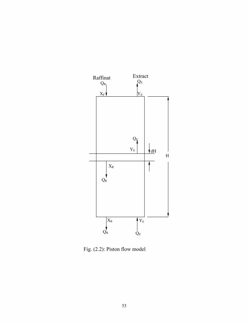
53

H

QE QR

QE QR

QE

QR

YE

YE

YE XR

XR

XF

dH

Raffinat Extract

Fig. (2.2): Piston flow model

54

and

221

.RMRM

avRCCC +

= (2.47)

where C refers to total concentration of all substances present in the

raffinate phase.

Better prediction of mass transfer efficiency has been shown to be

possible by including the effect of the axial mixing in the process of the

mass transfer modelling. Four such models are discussed below.

2.16.2 Stage Model

This is the simplest model to describe mass transfer with

longitudinal mixing in counter-current extraction columns Young (1957).

A diagrammatic representation of the model is shown in figure 2.3

In this model each stage is assumed to be perfectly mixed so that the

solute concentrations in streams leaving any stage are identical with those

in the same phase throughout the stage. Axial mixing is only

recommended for cases where the extent of the axial mixing in both

phases is similar and where its influence on the mass transfer is not high.

Miyauchi et al( 1963) considered that the model could only be used

when:

a) Interdroplet coalescence is frequent, or

b) The drop size distribution would narrow the distribution

coefficient m, hold-up, x and mass transfer coefficient k.

A material balance on ith stage is described by

( ) ( )iiEiR YYQXXQ −=− +− 111 (2.48)

and the mass transfer in the ith stage by

( )*1 ii

R

xii XX

QallKXX −=− − (2.49)

55

1

i-1

i

i+1

n

QEYE QRXF

QEYi

QEYi+1

QEYs

QRXi-1

QRXR

QRXi

Fig. (2.3): Stage flow model.

56

The boundary conditions are

snRn

EF

YYXX

YYXX

==

==

+1

0

Analytical solution is required for Equations (2.46) and (2.48) for the

linear case, and graphical solution required for the non-linear case

Sicicher(1959).

2.17 behaviour of drops in oil-water Emulsion

The behaviour of drops of oil as dispersed phase and water as a

continuous phase was investigated by Sajjadi (2000).Sajjadi observed

that. The size of internal oil droplets continuously decreased with time

until it reached a steady-state value., the size of multiple water drops

either reached a steady-state value or continued enlarging until

equilibrium He observed that by reducing the surfactant concentration,

the ability of the dispersed phase to entrain the continuous phase

decreased so that no minimum was achieved for the size of multiple drops

with time, similar to conventional systems with simple drops. The size

distribution of the multiple water drops initially narrowed and then

widened again, whereas the size distribution of internal oil droplets

continuously narrowed with time until it reached a constant value. The

possible mechanisms for complex drop formation were discussed and

drop deformation was suggested as the main cause for inclusion of a low

dispersed phase ratio Sajjadi (2000).

It was observed that the drop breakage rate dominates the drop

coalescence rate in the initial stage of stirring, which causes the drop

sizes to decrease with time , Arishman, et al (1980) .As stirring proceeds,

the drop breakage rate decreases while drop coalescence rate increases.

hence, a steady state is reached where the rate of both processes become

57

equal, and a steady-state drop size distribution is established. Hong and

Lee( 1983) indicated that the average drop size during the initial period of

mixing decreases exponentially while the size distribution changes less

drastically from wide to narrow. The effects of dispersed phase volume

fraction and surfactant concentration need to be studied and analyzed.

2.17.1 Analysis of drop The drop diameter, the Sauter diameter and polydispersity index

(PDI), were calculated by the following equations:

dn = ∑ni di / ∑ni (2.50)

ds= d32 = ∑ni di3 / ∑ni di

2 (2.51)

d32 = ∑ni di4 / ∑ni di

3 (2.52)

PDI = dw / dn (2.53)

Where ni is the number of drops with diameter di,. ds is equivalent

Sauter mean diameter, d32, generally used to analyze liquid-liquid

dispersion systems.

2.17.2 Drop size measurement The side of drops were measured by normal method of video camera by

sizing the drops from enlarge photos.

The procedure stated in details by sajjadi (2000).

2.18 Equipment Classification

There are two major categories of equipments for liquid extraction.

(A) Stagewise Contactors, in which liquids are mixed, extracted and

separated in discrete stages. This class includes the mixer

settler range of equipment.

(B) Differential Contactors, in which continuous counter-current

contact is established between the immiscible phase to give the

58

equivalent of any desired number of stages. These may be

categorised as

(1) Gravity Operated Extractors

(a) Non-mechanical dispersion

( I ) Baffle Plate Columns

(II ) Spray columns

(III) Packed columns

(IV) Perforated-plate columns

(b) Mechanically Agitated columns

( I ) Pulsed columns

(II ) Rotary Agitated Columns

( i ) The Rotating Disc Contactor

(ii ) The Schiebel Column

(iii) The Oldshue-Rushton Column

(iv ) The Assymetric Rotating Disc Contactor

A summary of the agitated column design is given in Table (2.5)

2.19 Selection of Equipment

Continuous contactors are generally preferable to mixer settlers

when large throughputs are to be handled since they offer economies in

agitation and power cost, floor space and solvent inventory. They

operate with relatively small amounts of hold-up of raffinate and extract.

This is important when processing radioactive flammable, expensive or

low stability materials. In extraction processes it is necessary as a final

step, or in multi-contact stagewise equipment, at intermediate steps, to

separate the two phases. Rapid coalescence is desirable otherwise an

excessive residence time is required or some of the continuous phase will

be removed with the ‘bulk’ dispersed phase, resulting in reduced

efficiencies, capacity and loss of solvent. Hence the contractor which

gives the most rapid solute transfer is not necessarily the most economic.

59

Continuous columns without mechanical agitation are unsuitable for

use with systems of high interfacial tension since adequate dispersions

cannot be achieved throughout continuous phase. Centrifugal extractors

have relatively high capital and operating costs and the number of stages

which can be accomodated in a single unit is limited. Nevertheless they

are superior to all other contactors for processes requiring a low hold-up

or low contact time, or if there is a low density difference between the

phases Khandel wal( 1978).

61

Table 2.5 Continuous Differential Contactors. Gurashi (1985)

Contactor Type Comment 1. RDC Contrally located dises driven in compariments

separated by stator rings by a central shaft. Operation reasonably flexible: efficiency notmuch affected by phase flow ratio: H.E.T.S. is remarkably low, around 20 per cent of that for a simple packed tower. Hydrodynamics and mass transfer characteristics are partially known.

2. A. R. D. C. Similar to the R. D. C. except that the rotor is off-set from the column axis; separations of phases take place in a shielded transfer section.

Fixing and separation zones claimed to reduce backmixing; but phase entrainment does occur in settling zone reducing overall efficiency. No special advantages over R.D.C.

3. Oldshue Rushton Vertical column divided into compartments by horizontal stator rings with vertical baffles in each compartment. Turbine in each compartment drive n by a central shaft.

Coalescence-redispersion is predominant. Stage efficiencies obtained by Oldshue and Rushton varied from 40 to 90%. H.E.T.S. was nearly half that of a simple packed tower of same diameter.

4. Ziel Extractor Vertical column terminating at top and bottom inlarge vessel to assist settling. The stirring mechanism consists of a shaft fitted with a number of star-shaped impellers. Vertical, reciprocal, as well as rotary motion is imposed on the impellers for effective mixing.

Theoretical efficiencies claimed to have been attained in the manufacture of phenol formaldehyde resin . No mass transfer data is available.

62

Table (Continued)

Contactor Type Comment 5. Scheibel Column Consists of alternate fully-baffled mixing

sections and packed sections. Agitation is provided by centrally located impellers.

Coalescence-redispersion is predominant. Mass transfer coefficient is related by

5.1

⎟⎟⎠

⎞⎜⎜⎝

⎛ ∇=

γecKa

Capacity is limited by permissible flow rate through the packing.

6. Khuni Extractor Incorporates the principles of R.D.C. Oldshue-Rushton and sieve plate columns. Divided into compartments by places perforated only at the centre so that flow from one compartment to the next is directed towards the agitator. Each compartment has four vertical baffles. Impeller agitatage for effective settling.

Published mass transfer data are limited. Capacity and scale-up are expressed by

05.06.061.0 ..Re. FrweCDd=

The design allows for only low through-puts. Modified designs have found limited application.

7. Pulsed Columns Phases are interdispersed by inducing a pulsating motion either by means of diaphragm pump or a valveless piston. A variety of internal packing or baffles may he used. In one design the plates are pulsed

Commercial application is limited. Empolyed in the extraction of metals from radioactive solutions. Power requirements are high. No published information is available for scale-up. Mass transfer data have been reported by various authors.

63

Table (2.6) Advantages and Disadvantages of Various Contractors. Logsadil (1971)

Space

Type

Capital

Cost

Operating and

Maintenance

Costs

Efficiency Total

Capacity

Flexibility Volumetric

Efficiency Vertical Floor

Ability to

Handle

Systems that

Emulsify

Spray Tower 5 5 1 2 2 1 0 5 3

Baffle Plate Tower 4 5 2 1 2 3 1 5 3

Packed Tower 4 5 2 2 2 2 1 5 3

R.D.C. 3 4 4 3 5 4 3 5 3

Pulsed Plate Column 3 3 4 3 4 4 3 5 1

Mixer settler 2 2 3 4 3 3 5 1 0

Centrifugal 1 2 5 3 5 5 5 5 5

0 = Unsuitable, 1 = poor, 2 = Fair, 3 = Adequate, 4 = Good, 5 = Outstanding (preferred

64

Table (2.6) is a useful ‘rule of thumb’ method for a preliminary

narrowing of the choice between the various types of extractor (Todd

1957). Special process factors often govern extractor selection .

Equipment installation and operating costs are of primary importance.

On this basis, and dependent on the number of stages for a given

application and the case of phase dispersion/separation, an extractor

selection chart can be drawn for any given feed rate range.

In general the choice of equipment for a given separation should be

based on the minimum annual cost for the complete plant, i.e., extractor

and ancillary equipment, as well as an operating and solvent loss costs.

Previously Logsdail (1971) has described the various design

considerations and process parameters to be considered in arriving at a

decision on solvent extraction equipment. The various factors and choice

of extractors are outlined in table (2.6).

2.20.1 Phase Equilibrium

In liquid extraction, the phase equilibrium of interest are those

showing the distribution of the solute( c ) between the two immiscible or

partially miscible liquids (A) and (S). in the case where the natural

solubility of liquids (A) and (S), even in the presence of the solute (C), is

negligible [immiscible liquids], the equilibrium becomes a simple relation

between the concentrations of the solute (C) in the two phases. The

equilibrium condition, is conveniently considered in terms of the

distribution law. Thus, at equilibrium:

The ratio of the concentrations of the solute in the two phases is

given by: ca

cs

xxK = (2.54)

Where K - distribution coefficient.

65

The equilibrium relation is easily shown by a plot of the

concentration of the solute in one phase against the concentration in the

other phase.

But, when the mutual solubility of the carrier (A) and solvent (S)

cannot be neglected; [partially miscible liquids]; the solubility and

equilibrium diagram, the limits of mutual solubility are marked by the

bimodal curve and the compositions the of phases in equilibrium by tie

lines. The region within the dome is two phase and that outside is one

phase. The miscibility boundary (saturation curve) can be obtained

experimentally by a cloud point titration. To obtain data to construct tie

lines, it is necessary to make a mixture (A, C, S), equilibrate it, and then

chemically analyze the resulting extract and raffinate phases. At the plait

point, the two liquid phases have identical composition. Each corner of

the triangular diagram represents a pure component.

This case is the most commonly encountered, and a number of phase

diagrams and computational techniques have been devised to determine the

equilibrium compositions. The graphical methods are still used to

represent equilibrium data and perform extraction calculations for ternary

systems. However, these methods are tedious and can't be used directly in

cases requiring computer analysis. Hence, methods for prediction of phase

equilibrium and correlation of tie line data have been developed.

2.20.2 Tie-line Correlations

In the case of many systems described in the literature, only a few

tie lines have been experimentally determined. Direct interpolation of

such data may lead to highly inaccurate results. Several tie line

correlations in equation four have been proposed (identified with these

subscripts):

CA = solute C in carrier phase A.

66

AA = carrier A in carrier phase A.

SA = solvent S in carrier phase A.

CS = solute C in solvent phase S.

AS = carrier A in solvent phase S.

SS = solvent S in solvent phase S.

2.20.3 Othmer and Tobias' Correlation

Othmer and Tobias have found that a plot of conjugate values of

AA

AA

xx1− against

SS

SS

xx1− on logarithmic coordinates produced straight lines

useful for interpolation and extrapolation Othmer, etal (1942):

n

AA

AA

SS

SS

xx1K

xx1

⎟⎟⎠

⎞⎜⎜⎝

⎛ −=

− (2.55)

These methods suffer from the fact that the concentration of the

distributed component (C) is not indicated in the coordinates.

2.20.4 Hand's Correlation

Hand showed that a logarithmic plot of AA

CA

XX against

SS

CS

XX (which

includes the concentration of the distributed component (C) in the

coordinates), gives generally a rectilinear plot. Hand's equation for the

correlation of tie-line data is ,Hand (1930),:

n

AA

CA

SS

CS

xxK

xx

⎟⎟⎠

⎞⎜⎜⎝

⎛= (2.56)

Furthermore, a simple method for estimating the entire equilibrium

diagram and locating the plait point based on this method has been

devised. If on the same graph as the tie-line data the bimodal curve is

plotted as S

C

XX against

A

C

XX , where XA, XC, and XS are concentrations of

the components at any point on the bimodal curve, a single curve of two

67

branches is obtained, one branch representing the A-rich layer and the

other the S-rich layer.

A the plait point, the distinction between the A-rich and the S-rich

phases disappears:

⎥⎥⎦

⎤

⎢⎢⎣

⎡⎟⎟⎠

⎞⎜⎜⎝

⎛=⎟⎟

⎠

⎞⎜⎜⎝

⎛=⎟⎟

⎠

⎞⎜⎜⎝

⎛

PS

C

PSA

CA

PSS

CS

XX

XX

XX and

⎥⎥⎦

⎤

⎢⎢⎣

⎡⎟⎟⎠

⎞⎜⎜⎝

⎛=⎟⎟

⎠

⎞⎜⎜⎝

⎛=⎟⎟

⎠

⎞⎜⎜⎝

⎛

PA

C

PAS

CS

PAA

CA

XX

XX

XX (2.57)

When subscript P represents the plait point. Since the plait point

represents a limiting line, the coordinates PAA

CA

XX

⎟⎟⎠

⎞⎜⎜⎝

⎛ and PSS

CS

XX

⎟⎟⎠

⎞⎜⎜⎝

⎛ must fall

simultaneously on the tie line correlation and on the bimodal curve.

Extrapolating the straight line tie-line correlation to intersect with the

solubility curve will locate the plait point.

2.20.5 Ishida's correlation:

Ishida's equation for the correlation of tie-line data is:

n

SSAA

SAAS

SSCA

CSSA

xxxxK

xxxx

⎟⎟⎠

⎞⎜⎜⎝

⎛= (2.58)

Where K ands n are constants. This equation should plot linearly

on logarithmic coordinates, Rod,(1966).

68

CHAPTER THREE

MATERIALS AND METHODS

3.1 Selection of Liquid-Liquid Chemical Systems

The system used in this work was oil –water-n.hexane which was

selected due to the following reasons:

1. Oil in water makes a serious pollution problem in the premices of

oil fields and refineries in Sudan.

2. the two solvents i.e., water and n-hexane are almost completely

immiscible.

3. the physical properties of the two systems such as density surface

tension, specific gravity, and viscosity are different.

4. the system is industrially and environmentally important.

5. the analysis of the liquid mixtures can be performed on various

devices such as liquid chromatographs, refractometers, and

electro-photometers.

6. the solute has a high selectivity in normal hexane.

7. equilibrium data could be obtained through experiments with

Smith-Bonner cell.

3.2 Sampling Procedures

Waste water samples were taken from main discharge channel which

leads the final waste water from Abugabra filed to the open area .The

sample of waste water were collected in 36 liters capacity plastic

containers .

The physical and chemical properties of n. hexane and waste water

were shown in appendix 2

69

3.3 Description of Equipment

The unit is a sieve tray column of 110cms in lengths ,30cms in

diameter and has 10 trays it was situated in the unit operation pilot

plant in Gezera University.

The body is provided with 9 stages. Each of which has a tray space.

An agitator shaft with blades is vertically arranged in the center of

column.

Heavy liquid and light liquid are supplied into the column interior

from the column top and bottom respectively by means of piston

pumps. These liquids make contact with each other inside the

column .mean while, the oil –water emulsion are mixed to small

drops in each stage with the solvent through agitation. Thus

permitting perfect mixing and better contact of the phases.

Volume of each feed liquid was controlled by adjusting the dial of

each pump. And The number of revolutions of the agitator shaft can

be controlled by manual adjustment

For the function of each section of the unit and the overall

assembled condition, see Figure.(3.1). This would Provide about 10

litters of fresh water in each tank to start test operation. Each pump

shall be Operated each pump to feed the fresh water into the system,

check if no leak of water takes place.

In case a leakage is observed, necessary countermeasures should be

taken. In most cases this problem can be solved by further fastening

of the piping and joints.

Operate the D.C. motor, increase the dial readings of revolving

controller gradually, starting from (0). In this case, take good care

not to operate the motor at a high rotating speed.

The fresh water thus fed into the system should be drained out. It

takes approximately an hour for complete drainage.

70

The capacity of each tank is 25 liters.

3.3. 1 Determination of flooding points:

Flooding is brought by excessive flow, causing liquid to be entrained

in vapour.

This is carried out without mass transfer

Procedure: The column was filled with the continuous phase and flow rate was

adjusted, and agitation was started at low speed of agitation (200

rpm).then, this is followed by:

Introducing the dispersed phase at low flow rate and continuouslly

increasing until flooding. Repeat 2 through 3 at different agitator

speed (200,300,500,and 600 rpm).

Increase the flow rate of the continuous phase, and repeat 2 through 4

The result is shown in figure (4.1) and table (4.1)

71

Fig. 3.1 Photo pilot plant sieve tray column

72

3.4 Experimentation Experiments to determine the transfer of oil from the aqueous

emulsion phase to n-hexane phase were performed, and phase's flow rates

were kept below 85% of flooding flow rates under non-mass transfer

conditions.

The procedure followed during these operations was:

Before starting experiments n-hexane was mutually saturated by

circulating it in closed loop for approximately 6 hours afterwards it was

left overnight to settle and separate, the column was then filled with the

continuous phase (oil-water emulsion), the agitator adjusted to the

required speed.

The dispersed phase n-hexane was introduced into the column and

its flow rate adjusted. The continuous phase was introduced into the

column and its flow rate adjusted to the required level.

After steady-state condition has been reached, about 20mintes

samples and photographs were taken for analysis. The same was repeated

at different flow rates at various solvent to liquid ratio, with and without

mass transfer, the speed of agitation was also varied.

3.5Determination of Equilibrium

Equilibrium concentrations were determined by making up mixtures

on weight basis to represent points below the solubility curve.

Each mixture was contained in Smith-Bonner cell and brought to

equilibrium through agitation and standing for several hours. The layers

were then separated using separating funnel and sample were analyzed

using the electro photometer.

Determination of Sauter mean diameter: Digital camera was

employed for this photography. Three photographs were taken for each

events and then used a hand lens (x4) and venire caliper to count the

73

number of drops and the diameter of each drop was determined. Result

shown in tables (4.2) up to (4.17)

3.6 Calculation Method

3.6.1 Experimental mass transfer coefficient

The over all experimental dispersed phase mass transfer coefficient

under each set of operating conditions was calculated using

( )mCKAN ∆= (3.1)

where N is the mass transfer rate

VaA ∗= (3.2)

32

6d

xa = (3.3)

where a is specific interfacial area in cm2 per cm3 of the column

volume, and v is the column volume. Simpson rule was applied to

determine the actual mean driving force ( )mC∆ by using the oil

concentration profile a long the column. Oil concentration was

determined in samples of continuous phase taken from trays number 1,2,3

up to 7, the driving force in these trays can be determine as 1y∆ , 2y∆ , 3y∆

and 7y∆ respectively, where

yyy −=∆ * (3.4)

and y is the oil concentration of aqueous phase so Simpson's rule is:

{ })(2)(4181

53642 yyyyyyyy bottopm ∆+∆+∆+∆+∆+∆+∆=∆

(3.5)

my∆ was then converted to mC∆ by dividing it by the extract phase density,

so the over all experimental mass transfer coefficient can be calculated as

mCA

NK∆

=exp (3.6)

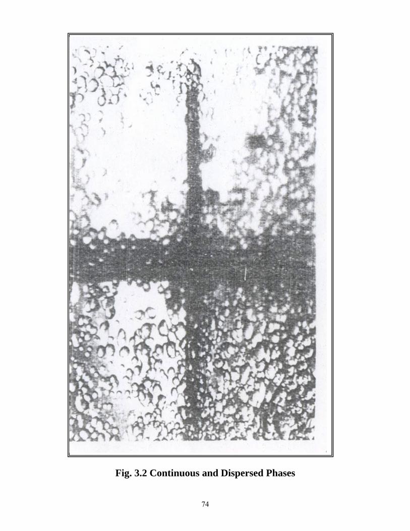
74

Fig. 3.2 Continuous and Dispersed Phases

75

3.6.2 Theoretical mass Transfer Coefficient

The method of calculation of dispersed phase transfer coefficient

Kcal was used, these calculations involve the use of the drop distribution

diagram to determine the volume percentage of stagnant, circulating and

oscillating drops, in drop swarms. Sample population, and Droplet

Reynolds number have been used as a measure of the state of drops, as

follows :

Stagnant drops Re < 10

Circulating drops 10 < Re < 200

Oscillating drops Re > 200

Where droplet Reynolds number is:

c

cVdµρ.Re = (3.7)

where d is the drop diameter and Vc is vertical relative velocity of

drops determined by applying Misek equation:

⎥⎦⎤

⎢⎣⎡

−+=

xV

xVV Cd

C 1 (3.8)

To find the maximum diameter of stagnant drops in the whole drop population:

set Re = 10

10=ccVds c

µρ (3.9)

where ds is maximum diameter of the stagnant drops regime, to find the minimum diameter of oscillating drops in the oscillating drop regime:

set Re = 200

2000

=µρ ccVdo (3.10)

where do is the minimum diameter of the oscillating drops regime. The circulating drops regime is determined some what between ds and do, the stagnant drops are too small to be analyzed by the technique used in this study, so the drop population was considered to contain circulating

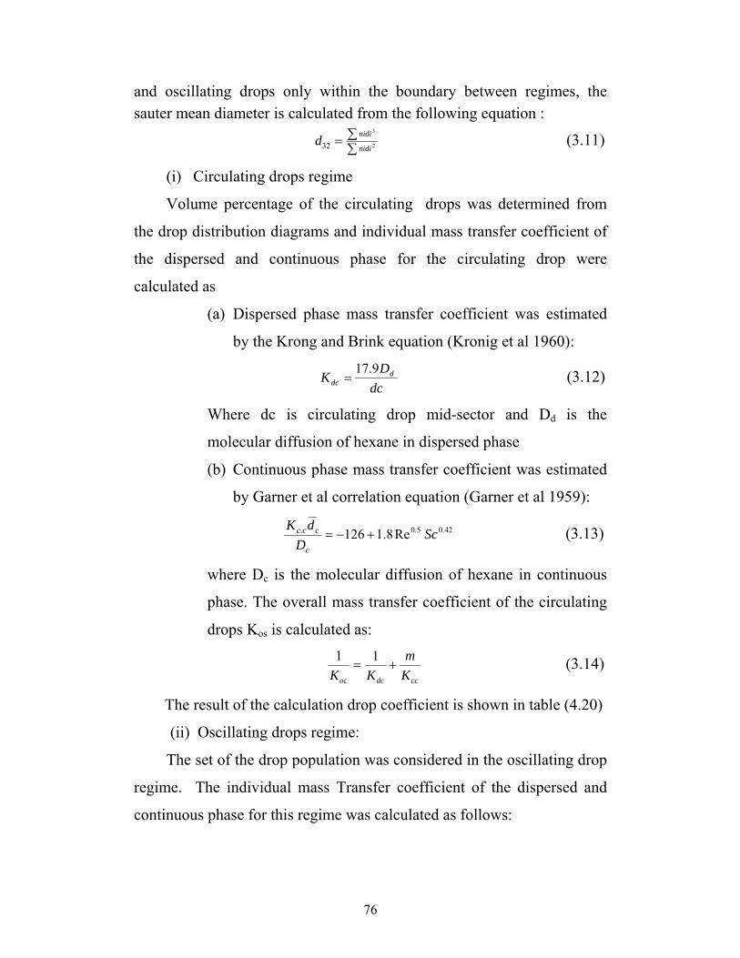
76

and oscillating drops only within the boundary between regimes, the sauter mean diameter is calculated from the following equation :

∑∑= 2

3

32 nidi

nidid (3.11)

(i) Circulating drops regime

Volume percentage of the circulating drops was determined from

the drop distribution diagrams and individual mass transfer coefficient of

the dispersed and continuous phase for the circulating drop were

calculated as

(a) Dispersed phase mass transfer coefficient was estimated

by the Krong and Brink equation (Kronig et al 1960):

dc

DK d

dc9.17

= (3.12)

Where dc is circulating drop mid-sector and Dd is the

molecular diffusion of hexane in dispersed phase

(b) Continuous phase mass transfer coefficient was estimated

by Garner et al correlation equation (Garner et al 1959):

42.05.0. Re8.1126 ScD

dK

c

ccc +−= (3.13)

where Dc is the molecular diffusion of hexane in continuous

phase. The overall mass transfer coefficient of the circulating

drops Kos is calculated as:

ccdcoc K

mKK

+=11 (3.14)

The result of the calculation drop coefficient is shown in table (4.20)

(ii) Oscillating drops regime:

The set of the drop population was considered in the oscillating drop

regime. The individual mass Transfer coefficient of the dispersed and

continuous phase for this regime was calculated as follows:

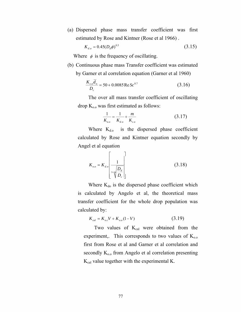
77

(a) Dispersed phase mass transfer coefficient was first estimated by Rose and Kintner (Rose et al 1966) .

5.0. )(45.0 φdod DK = (3.15)

Where φ is the frequency of oscillating.

(b) Continuous phase mass Transfer coefficient was estimated by Garner et al correlation equation (Garner et al 1960)

7.0. Re0085.050 ScD

dK

c

ooc += (3.16)

The over all mass transfer coefficient of oscillating drop Ko.o was first estimated as follows:

ocodoo K

mKK ...

11+= (3.17)

Where Kd.o is the dispersed phase coefficient calculated by Rose and Kintner equation secondly by Angel et al equation

⎥⎥⎥⎥⎥

⎦

⎤

⎢⎢⎢⎢⎢

⎣

⎡

=+m

c

dodoo

DD

KK1

..1 (3.18)

Where Kdo is the dispersed phase coefficient which is calculated by Angelo et al, the theoretical mass transfer coefficient for the whole drop population was calculated by:

)1(.. VKVKK oococal −+= (3.19)

Two values of Kcal were obtained from the experiment,. This corresponds to two values of Ko.o first from Rose et al and Garner et al correlation and secondly Ko.o from Angelo et al correlation presenting Kcal value together with the experimental K.

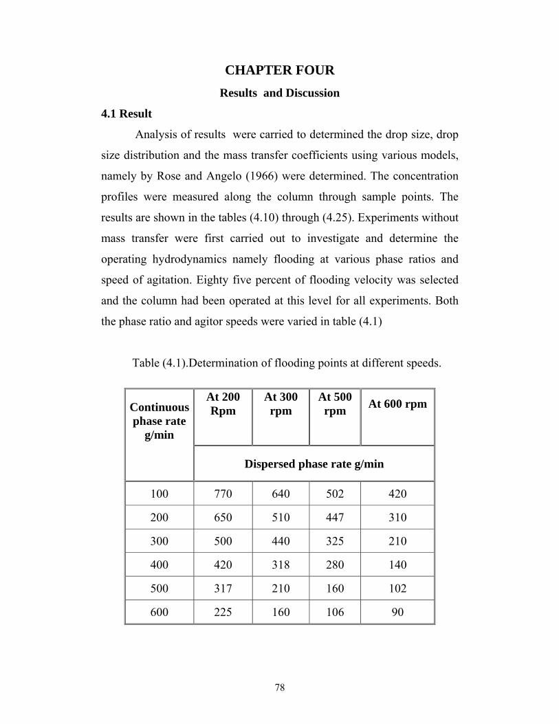
78

CHAPTER FOUR Results and Discussion

4.1 Result

Analysis of results were carried to determined the drop size, drop

size distribution and the mass transfer coefficients using various models,

namely by Rose and Angelo (1966) were determined. The concentration

profiles were measured along the column through sample points. The

results are shown in the tables (4.10) through (4.25). Experiments without

mass transfer were first carried out to investigate and determine the

operating hydrodynamics namely flooding at various phase ratios and

speed of agitation. Eighty five percent of flooding velocity was selected

and the column had been operated at this level for all experiments. Both

the phase ratio and agitor speeds were varied in table (4.1)

Table (4.1).Determination of flooding points at different speeds.

At 200 Rpm

At 300 rpm

At 500 rpm

At 600 rpm

Continuous phase rate

g/min Dispersed phase rate g/min

100 770 640 502 420

200 650 510 447 310

300 500 440 325 210

400 420 318 280 140

500 317 210 160 102

600 225 160 106 90

79

Fig.(4.1) Flooding points at different phase ratio and various agitator

speeds(without mass transfer)

0

100

200

300

400

500

600

700

800

900

100 200 300 400 500 600

continuos phase rate (g/min)

disp

erse

d ph

ase

rate

(g/m

in)

at 200 rpmat 300 rpmat 500 rpmat 600 rpm

80

Table (4.2) Drop size, number of drops and Cumulative volume at

200 rpm(without mass transfer)

dm mm

d mm n V

mm3 1.400 1.0570 2 1.2367

2.5900 1.2950 4 4.5462 3.1400 1.5700 3 6.0757 3.700 1.8500 6 19.8813

5.3500 2.6750 7 70.1210 7.0100 3.5050 10 225.3422 6.1800 3.0900 9 466.4100 7.5600 3.7800 8 692.6472 7.8400 3.9200 10 1008.0437 8.1100 4.0550 7 1252.4257 8.1900 4.0950 8 1540.0664

Where:

dm: Measured Diameter

d: Actual Diameter

n: Number of Drops

V: Cumulative Volume

Cumulative drop volume 36

dnV ×= π

Phase ratio = 1: 0.8

Magnification= 2

81

Table (4.3) Determination of Sauter mean diameter (d32)Agitator

Speed 200 rpm(without mass transfer)

dmm d2

mm2

d3

mm3

n nd2

mm2

nd3

mm3

1.0570 1.1172 1.1809 2 2.2344 2.3618

1.2950 1.6770 1.1717 4 6.7080 4.6868

1.5700 2.4645 3.8699 3 7.3935 11.9097

1.8500 3.4225 6.3316 6 20.5350 37.9896

2.6750 7.1556 19.1413 7 50.0892 133.9891

3.5050 12.2850 43.0590 10 122.8500 430.5900

3.0900 9.5481 29.5036 9 85.9325 265.5324

3.7800 14.2884 54.0102 8 114.3072 432.0816

3.9200 15.3664 60.2363 10 153.6640 602.3630

4.0550 16.4430 66.6765 7 115.1010 466.7355

4.0150 16.1202 64.7272 8 128.9618 517.7816

807.7766 2906.021

d32 =3.5975

82


300 rpm (without mass transfer)

dm mm

d mm n

V

mm3

2.0400 1.0200 4 2.2226

3.1400 1.5700 5 12.3540

3.700 1.8500 5 28.9302

4.8000 2.4000 3 50.6449

5.3200 2.6750 9 140.8461

3.9000 2.9500 10 275.2663

6.1800 3.0900 6 367.9547

6.4600 3.2300 8 509.1097

7.0100 3.505 5 621.8379

7.5600 3.780 5 763.2361

8.1100 4.0550 6 972.7064

8.1900 4.0950 5 1152.4818

83

Table (4.5)Determination of Sauter mean diameter (d32)Agitator


dmm d2

mm2

d3

mm3

n nd2

mm2

nd3

mm3

1.0200 1.0404 1.0612 4 4.1616 4.2448

1.5700 2.4649 3.8699 5 12.32415 19.3495

1.8500 3.4225 6.3316 5 1.1125 31.6580

2.4000 5.7600 13.8240 3 17.28 41.4720

2.6750 7.1556 19.1413 9 64.4004 172.2717

2.9500 8.7025 25.6724 10 87.025 256.724

2.0900 4.3681 9.1293 6 26.2086 54.7758

3.23 10.4329 33.6982 8 83.4632 269.5856

3.5050 12.8503 43.0590 5 64.2515 215.295

3.7800 14.2884 54.0102 5 71.442 270.051

4.0550 16.4430 66.6765 6 98.658 400.059

4.0950 16.7690 68.6692 5 83.8450 343.346

614.172 2078.8324

d32 = 3.384773 mm

84


500 rpm (without mass transfer)

dm mm

d mm

n V

mm3

2.0400 1.0200 13 7.2234

3.1400 1.5700 9 25.4598

3.7000 1.8500 10 58.6121

4.2900 2.1450 8 99.9521

4.8000 2.400 7 150.6196

5.3500 2.6750 4 190.7090

6.1800 3.0900 8 314.2935

7.0100 3.5050 4 404.4761

7.5604 3.7805 3 431.4919

8.1100 4.055 2 501.3153

8.3900 4.1950 2 578.6233

8.66 4.3300 3 706.14484

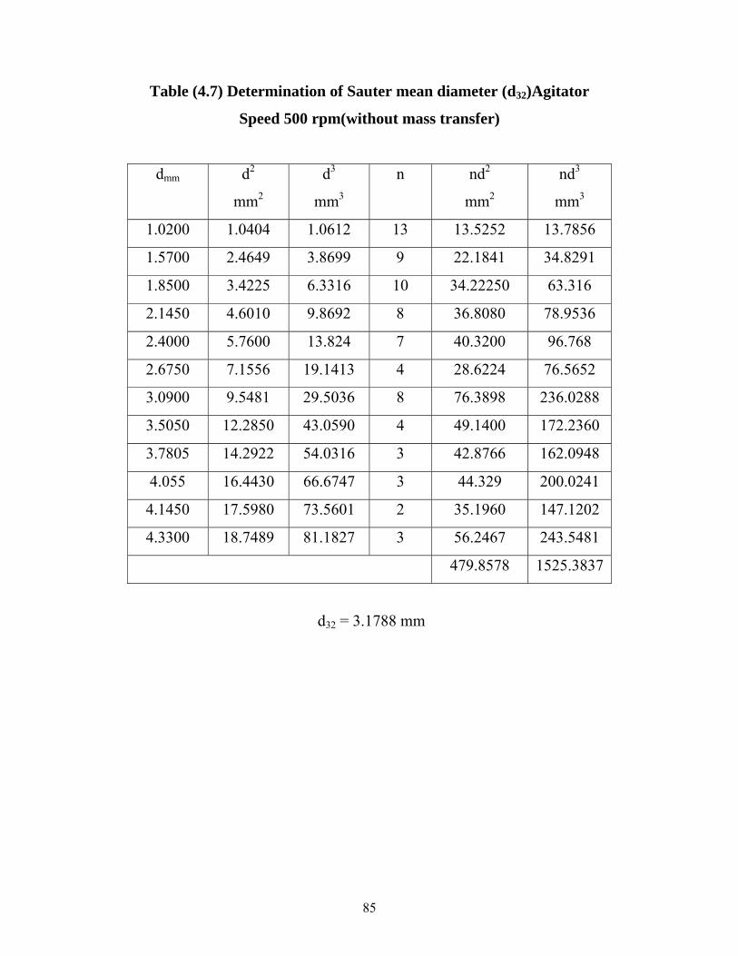
85



dmm d2

mm2

d3

mm3

n nd2

mm2

nd3

mm3

1.0200 1.0404 1.0612 13 13.5252 13.7856

1.5700 2.4649 3.8699 9 22.1841 34.8291

1.8500 3.4225 6.3316 10 34.22250 63.316

2.1450 4.6010 9.8692 8 36.8080 78.9536

2.4000 5.7600 13.824 7 40.3200 96.768

2.6750 7.1556 19.1413 4 28.6224 76.5652

3.0900 9.5481 29.5036 8 76.3898 236.0288

3.5050 12.2850 43.0590 4 49.1400 172.2360

3.7805 14.2922 54.0316 3 42.8766 162.0948

4.055 16.4430 66.6747 3 44.329 200.0241

4.1450 17.5980 73.5601 2 35.1960 147.1202

4.3300 18.7489 81.1827 3 56.2467 243.5481

479.8578 1525.3837

d32 = 3.1788 mm

86


600 rpm(without mass transfer)

dm mm

d mm

n V

mm3

1.4900 0.7450 20 4.3301

2.0400 1.0200 15 12.6648

2.5900 1.2950 20 35.4073

3.1400 1.7500 8 51.6175

3.7000 1.8500 12 91.4003

2.2500 2.1250 3 106.4732

4.8000 2.400 2 120.9497

5.3500 2.6750 3 151.0167

5.9000 2.950 2 177.9007

6.1800 3.0900 3 224.2448

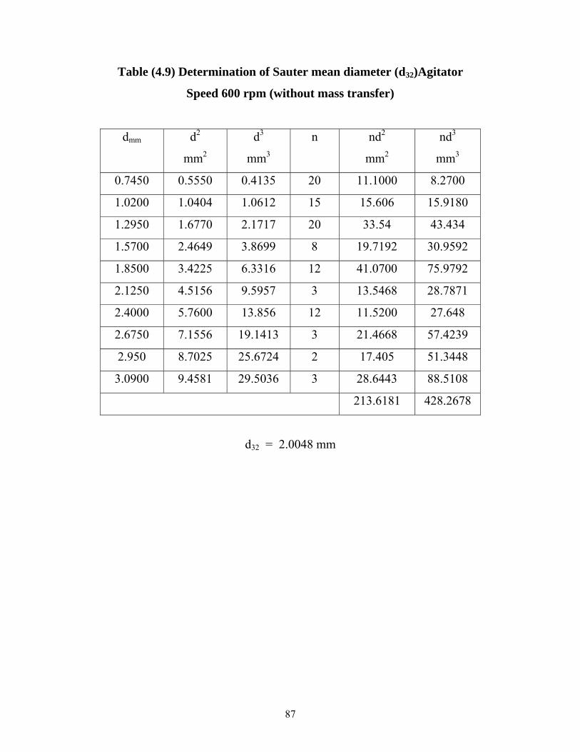
87


Speed 600 rpm (without mass transfer)

dmm d2

mm2

d3

mm3

n nd2

mm2

nd3

mm3

0.7450 0.5550 0.4135 20 11.1000 8.2700

1.0200 1.0404 1.0612 15 15.606 15.9180

1.2950 1.6770 2.1717 20 33.54 43.434

1.5700 2.4649 3.8699 8 19.7192 30.9592

1.8500 3.4225 6.3316 12 41.0700 75.9792

2.1250 4.5156 9.5957 3 13.5468 28.7871

2.4000 5.7600 13.856 12 11.5200 27.648

2.6750 7.1556 19.1413 3 21.4668 57.4239

2.950 8.7025 25.6724 2 17.405 51.3448

3.0900 9.4581 29.5036 3 28.6443 88.5108

213.6181 428.2678

d32 = 2.0048 mm

88

Table (4.10) Drop size, number of drops and Cumulative volume at 200

rpm(with mass transfer)

dm mm

d mm n

V

mm3

1.49 0.745 3 0.6495

2.0400 1.0200 3 2.3164

2.5900 1.2950 4 6.849

3.4200 1.7100 5 19.9554

3.7000 1.850 5 36.5316

6.18 3.0900 6 129.2200

7.1000 3.5500 11 386.8974

7.2800 3.6400 8 5880.9167

7.5600 3.7800 10 871.7132

7.8400 3.9200 7 1092.4907

8.1100 4.055 8 1371.7844

8.3900 4.1950 7 1642.36244

8.66 4.3300 12 2152.4486

8.94 4.4700 16 2390.6209

89

Table (4.11) Determination of Sauter mean diameter (d32) Agitator

Speed 200 rpm(with mass transfer)

dmm d2

mm2

d3

mm3 n

nd2

mm2

nd3

mm3

0.745 0.5550 0.4135 3 1.6650 1.2405

1.0200 1.0404 1.0612 3 3.1212 3.1836

1.2950 1.6770 2.1717 4 6.708 8.6868

1.7100 2.9241 5.0002 5 14.6205 25.0010

1.850 3.4225 6.3316 5 17.1125 31.658

3.0900 9.5481 29.5036 6 57.2886 177.0216

3.5500 12.6025 44.7389 11 138.6275 492.1279

3.6400 13.2496 48.2285 8 105.9968 38.828

3.78 14.2884 54.0102 10 142.8840 540.102

3.92 15.3664 60.2363 7 107.5648 421.6541

4.055 16.4430 66.6765 8 131.5940 533.412

4.1950 17.5980 73.8237 7 123.1860 516.7659

4.33 18.7489 81.1827 12 224.9868 974.1424

4.47 19.9809 89.3146 16 319.6944 1429.0336

1451.208 5539.4074

d32 = 3.817101 mm

90

Table (4.12)Drop size, number of drops and Cumulative volume at 300

rpm (with mass transfer)

dm mm

d mm n

V

mm3

2.5900 1.2950 1 1.1240

3.1400 1.5700 7 15.3079

3.700 1.8500 8 41.8297

4.2500 2.1250 10 92.0727

4.8000 2.4000 8 149.9785

5.1900 2.5950 7 214.0270

3.3500 1.6750 24 273.0817

6.4600 3.2300 15 537.7473

7.0100 3.505 9 740.6581

7.5600 3.7800 3 825.4970

8.1100 4.0550 2 895.3204

8.6600 4.3300 3 1022.8414

91

Table (4.13) Determination of Sauter mean diameter (d32) Agitator

Speed 300 rpm (with mass transfer)

dmm d2

mm2

d3

mm3

n nd2

mm2

nd3

mm3

1.2950 1.6770 2.1717 2 1.6770 2.1717

1.5700 2.4649 3.8699 7 17.2543 27.0893

1.8500 3.4225 6.3316 8 27.3800 50.6528

2.1250 4.5156 9.5957 10 45.1560 95.9570

2.4000 5.7600 13.824 8 46.08 110.592

2.5950 6.7340 17.4748 7 47.1380 122.3236

1.6750 2.8056 4.6994 24 67.3344 112.7856

3.2300 10.4329 33.6982 15 156.4935 505.473

3.505 12.2850 43.590 9 110.5650 387.531

3.7800 14.2889 54.0402 3 42.8652 162.0306

4.0550 16.4430 66.6747 2 32.8860 133.3494

4.33 18.7489 81.1827 3 56.2467 243.5481

651.2964 1953.5046

d32 = 2.9994 mm

92



dm mm

d mm

n V

mm3

2.59 1.2950 14 15.91973

3.1400 1.5700 10 36.1824

3.1700 1.5850 17 71.6280

3.70000 1.8500 10 104.7803

4.2300 2.1150 12 164.2247

5.350 2.6750 3 194.2917

5.9000 2.9500 5 261.5018

6.4600 3.2300 4 305.0781

7.0100 3.5050 3 327.6237

93

Table (4.15)Determination of Sauter mean diameter (d32)Agitator Speed

500 rpm(with mass transfer)

dmm d2

mm2

d3

mm3

n nd2

mm2

nd3

mm3

1.2950 1.6770 2.1717 14 23.478 30.4038

1.5700 2.4649 3.8899 10 24.349 38.6990

1.5850 2.5122 3.9819 17 42.7074 67.6923

1.8500 3.4225 6.3316 10 34.2250 63.31600

2.1150 4.4732 9.4609 12 53.6784 113.5308

2.6750 7.1556 19.1413 3 21.4668 57.4239

2.950 8.7025 25.6724 5 43.5125 128.362

3.23 10.4329 33.6982 4 41.7316 134.7928

3.5050 12.2850 43.0590 3 37.755 129.177

323.2037 763.3976

d32 = 2.3619 mm

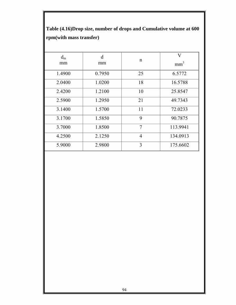
94



dm mm

d mm n

V

mm3

1.4900 0.7950 25 6.5772

2.0400 1.0200 18 16.5788

2.4200 1.2100 10 25.8547

2.5900 1.2950 21 49.7343

3.1400 1.5700 11 72.0233

3.1700 1.5850 9 90.7875

3.7000 1.8500 7 113.9941

4.2500 2.1250 4 134.0913

5.9000 2.9800 3 175.6602

95


Speed 600 rpm (with mass transfer)

dmm d2

mm2

d3

mm3

n nd2

mm2

nd3

mm3

0.7950 0.6320 0.5025 25 15.8000 12.5625

1.0200 1.0404 1.0612 8 18.7272 19.1016

1.2100 1.4641 1.7716 10 14.641 17.716

1.2950 1.6770 2.1717 21 35.217 451.057

1.7500 2.4649 3.8699 11 27.1139 42.5689

1.5850 2.5122 3.9819 9 22.6098 35.8371

1.8500 3.4225 6.3316 7 23.9575 44.3212

2.1250 4.5156 9.5957 4 18.0624 38.3828

2.9800 8.8804 26.4836 3 26.6412 79.4508

202.765 335.5538

d32 = 1.6548 mm

96

Table . (4.18)Experimental Mass Transfer Results

Run

No.

N

gm/s

d32

cm

Interfacial

Area cm2

Cm

gm/cm3

KEXP

cm/s

1 3.67 0.38171 73334.7 0.0206 3.59 × 10 -3

2 1.87 0.29994 9469.07 0.008 3.01 × 10 -3

3 1.62 0.23619 63245.88 0.0129 3.10 × 10 –3

4 1.35 0.16548 230601.6 0.0119 3.34 × 10 –3

5 1.60 0.3575 49765.86 0.0109 3.32 × 10 –3

6 3.80 0.33847 82660.5 0.0109 3.42 × 10 –3

7 5.38 0.31788 71978.22 0.0139 2.92 × 10 -3

Where :

N = Rate of mass transfer.

∆Cm = The mean driving force.

KEXP = Mass transfer coefficient.

Specific interfacial area 32

6d

xa =

Total interfacial area A = a .v

mCAN∆×

=EXPK

97

Table . (4.19)Theoretical Mass Transfer Results ,Result of Calculation

of V0 and ds and d0

Run

No.

Dispersed

phase

Vo

cm/sec

ds

cm

do

cm

1 n-hexane 9.143 0.015 0.303

2 “ 8.51 0.012 0.240

3 “ 9.62 0.0106 0.212

4 “ 9.44 0.0103 0.205

5 “ 10.14 0.00100 0.200

6 “ 10.36 0.0098 0.197

7 “ 10.45 0.0097 0.195

Where:

ds = Diameter of stagnant drop.

do = Diameter of oscillating drop.

The vertical relative velocity of drops ⎥⎥⎦

⎤

⎢⎢⎣

⎡

−+=

Xcv

Xdv

oV1

98

Table . (4.20) Mass Transfer Results

Circulating drop mass transfer coefficient

Run

No.

Dispersed

phase

Kdc

Cm/sec

Kcc

cm/sec

Koc

cm/sec

1 n-hexane 9.6×10 –6 1.26×10 –3 9.53×10 –6

2 “ 1.26×10 –5 1.56×10 -3 1.25×10 -5

3 “ 1.37×10 –5 1.73×10 -3 1.36×10 -5

4 “ 1.47×10 –5 1.85×10 -3 1.46×10 -5

5 “ 1.8×10 –5 2.54×10 –3 1.79×10 –3

6 “ 2.27×10 –5 2.24×10 -3 2.25×10 -5

7 “ 2.23×10 -5 2.28×10 –3 2.21×10 -5

Where:

Kdc = Dispersed phase mass transfer coefficient of circulating drop.

Kcc = Continuous phase mass transfer coefficient of circulating drop.

Koc = Overall mass transfer coefficient of circulating drop.

99

Table . (4.21) Mass Transfer Results

Comparison between mass transfer coefficient

With different models

Rose et al Angelo et al Run

No. Dispersed

phase Kd0 K0.0 K0.0 Kd.0

1 n-hexane 2.78×10 -3 4.03×10 –5 3.31×10 –3 2.8×10 –3

2 - 3.93×10 –3 3.93×10 -6 3.53×10 -3 7.14×10 –3

3 - 2.87×10 –3 2.87×10 -3 3.82×10 -3 7.72×10 –3

4 - 2.94×10 –3 2.94×10 -3 3.90×10 -3 7.88×10 -3

5 - 1.92×10 –3 1.91×10 –3 2.62×10 –3 5.30×10 –3

6 - 3.02×10 –3 3.21×10 -3 3.99×10 -3 8.07×10 –3

7 - 2.67×10 –3 2.23×10 –3 4.02×10 -3 8.14×10 -3

Where:

Kdo = Dispersed phase mass transfer coefficient of oscillating drop.

Koo = Overall mass transfer coefficient of oscillating drop.

100

Table . (4.22) Mass Transfer Results, Comparison between mass

transfer coefficient with various conditions

Kexp

Cm/sec

Kdc

cm/sec

Kcc

cm/sec

Koc

cm/sec

Kdo

Rose et al

Kdo

Angelo et al

×3.59 10 -3 9.6×10 -6 1.26×10 -3 9.53×10 -6 2.78×10 -3 2.8×10 -3

3.01×10 -3 1.2×10 –5 1.56×10 -3 1.25×10 -5 3.93×10 -3 7.14×10 -3

3.10×10 -3 1.37×10 –5 1.73×10 -3 1.36×10 -5 2.87×10 -3 7.72×10 -3

3.34×10 -3 1.47×10 –5 1.80×10 -3 1.46×10 -3 2.94×10 -3 7.88×10 -3

3.32×10 -3 2.27×10 –5 2.04×10 -3 1.79×10 -3 1.42×10 -3 5.30×10 -3

3.42×10 -3 1.8×10 –5 2.29×10 -3 2.25×10 -3 3.02×10 -3 8.07×10 -3

2.92×10 -3 2.23×10 –5 2.28×10 -3 2.21×10 -3 2.67×10 -3 8.14×10 -3

101

Table No. (4.23) Experimental and theoretical over mass transfer

coefficient

Run

No.

Kexp

cm/sec

Kcal

Rose and Garner

Kcal

Angelo et al

1 3.59×10 -3 3.11×10 -5 2.32×10 -3

2 3.01×10 -3 8.74×10 -6 2.97×10 -3

3 3.10×10 -3 1.48×10 -3 2.68×10 -3

4 3.34×10 -3 1.49×10 -3 3.17×10 -3

5 3.32×10 -3 1.87×10 -3 2.27×10 -3

6 3.42×10 -3 1.55×10 -3 2.79×10 -3

7 2.92×10 -3 1.57×10 -3 2.82×10 -3

Where:

Kcal = Calculated mass transfer coefficient.

102

Table. (4.24) Comparison between experimental and theoretical

mass Transfer coefficients

Dispersed

phase

Kexp

KCal

Rose

Kexp

KCal

Angelo

Kexp

K0.0

Angelo

Kexp

K0.0

Rose

n-hexane 115.43 1.54 1.08 89.08

“ 344.39 1.01 0.85 421.56

“ 2.09 1.15 0.81 1.49

“ 2.24 1.05 0.85 1.57

“ 1.77 1.46 1.26 1.73

“ 2.20 1.22 0.85 1.54

“ 1.85 1.03 0.72 0.76

103

Table .(4.25) Mass Transfer Results

Comparison between experimental and theoretical mass

Transfer coefficients

Run No.

Kexp Cm/sec

Kcal by Rose cm/sec

Kcal by Angelo

cm/sec

Kexp-kcal ×100 Kexp Rose

Kexp-kcal ×100Kexp

Angelo 1 3.59×10 -3 3.11×10 -5 2.32×10 -3 99.13 % 35.37 %

2 3.01×10 -3 8.73×10 -6 2.97×10 -3 99.75 1.32

3 3.10×10 -3 1.45×10 -3 2.68×10 -3 53.22 13.54

4 3.34×10 -3 1.44×10 -3 3.17×10 -3 55.38 5.08

5 3.32×10 -3 1.87×10 -3 3.27×10 -3 43.67 1.50

6 3.42×10 -3 1.55×10 -3 2.29×10 -3 54.67 18.42

7 2.92×10 -3 1.57×10 -3 2.82×10 -3 46.23 3.42

4.2 Discussions In general the waste water from oil fields and refineries has

considerable amount of crude oil fields in an emulsified and tiny floating

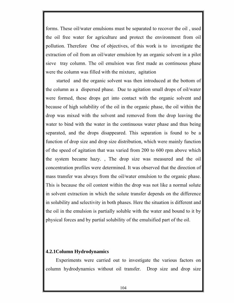
104

forms. These oil/water emulsions must be separated to recover the oil , used

the oil free water for agriculture and protect the environment from oil

pollution. Therefore One of objectives, of this work is to investigate the

extraction of oil from an oil/water emulsion by an organic solvent in a pilot

sieve tray column. The oil emulsion was first made as continuous phase

were the column was filled with the mixture, agitation

started and the organic solvent was then introduced at the bottom of

the column as a dispersed phase. Due to agitation small drops of oil/water

were formed, these drops get into contact with the organic solvent and

because of high solubility of the oil in the organic phase, the oil within the

drop was mixed with the solvent and removed from the drop leaving the

water to bind with the water in the continuous water phase and thus being

separated, and the drops disappeared. This separation is found to be a

function of drop size and drop size distribution, which were mainly function

of the speed of agitation that was varied from 200 to 600 rpm above which

the system became hazy. , The drop size was measured and the oil

concentration profiles were determined. It was observed that the direction of

mass transfer was always from the oil/water emulsion to the organic phase.

This is because the oil content within the drop was not like a normal solute

in solvent extraction in which the solute transfer depends on the difference

in solubility and selectivity in both phases. Here the situation is different and

the oil in the emulsion is partially soluble with the water and bound to it by

physical forces and by partial solubility of the emulsified part of the oil.

4.2.1Column Hydrodynamics

Experiments were carried out to investigate the various factors on

column hydrodynamics without oil transfer. Drop size and drop size

105

distribution were studied at different agitator speed (200 – 600 rpm) at

specified feed rates and phase ratios. The results indicated that drop size

decreased with agitator speed which is in agreement with all previous works.

Initially large drop size were dominant at low speeds, but still drop size

appeared, such drops might be due to the fact that these were the smallest

drop, which did not undergo any change as their size were already

established and could not be further subdivided into smaller drops.

However, upon increasing the agitator speed, the smaller size droplets

become dominant and i creased in population, this decrease in drop size

continued to decrease with speed of agitation, until a maximum speed was

reached (600 rpm) when the drop size could no longer be reduced. Any

further increase in the agitator speed will make the system milky and hazy

and at further speeds flooding occur, flooding was defined by phase ratio

n.hexane/emulsion in all cases i.e. at all feed rates, phase ratios with either

phase dispersed, the agitator speed played a controlling point with regard to

the flooding determination and as the phase ratio increased, flooding

occurred at a comparatively lower speed, the same effect was realized with

the feed rate i.e. as the feed rate increased.

A difference was clearly seen, when comparing the agitator speed at

which flooding occurred with respect to each dispersion, and when emulsion

was dispersed, flooding occurred at higher speed than that producing

flooding when n.hexane was dispersed at same conditions. This is because

the agitator speed needs more energy to disperse the heavy phase than that

required to disperse the light phase, hence flooding occurred at higher

speed.

The centrifugal action of the agitator tended to make the light phase

flow to the centre of the column and when the heavy phase was dispersed it

was necessary to overcome, the centrifugal action by setting up a high

velocity flow pattern to bring the heavy phase into the area in which the

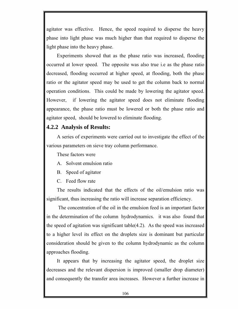
106

agitator was effective. Hence, the speed required to disperse the heavy

phase into light phase was much higher than that required to disperse the

light phase into the heavy phase.

Experiments showed that as the phase ratio was increased, flooding

occurred at lower speed. The opposite was also true i.e as the phase ratio

decreased, flooding occurred at higher speed, at flooding, both the phase

ratio or the agitator speed may be used to get the column back to normal

operation conditions. This could be made by lowering the agitator speed.

However, if lowering the agitator speed does not eliminate flooding

appearance, the phase ratio must be lowered or both the phase ratio and

agitator speed, should be lowered to eliminate flooding.

4.2.2 Analysis of Results: A series of experiments were carried out to investigate the effect of the

various parameters on sieve tray column performance.

These factors were

A. Solvent emulsion ratio

B. Speed of agitator

C. Feed flow rate

The results indicated that the effects of the oil/emulsion ratio was

significant, thus increasing the ratio will increase separation efficiency.

The concentration of the oil in the emulsion feed is an important factor

in the determination of the column hydrodynamics. it was also found that

the speed of agitation was significant table(4.2). As the speed was increased

to a higher level its effect on the droplets size is dominant but particular

consideration should be given to the column hydrodynamic as the column

approaches flooding.

It appears that by increasing the agitator speed, the droplet size

decreases and the relevant dispersion is improved (smaller drop diameter)

and consequently the transfer area increases. However a further increase in

107

the agitator speed did not increase the interfacial area as a uniform drop size

had been already established.

4.2.3 Experimental mass transfer coefficient

The overall experimental dispersed phase mass transfer coefficients

recorded in this study were evaluated by Simpson's rule. Simpson's rule has

a great advantage over the log-mean driving force in the agitated colum.The

agitator speed causes more the drop to break-up and the proportion of the

small droplets will be greater while the mass transfer coefficient become

smaller, with the result that stagnant or circulating droplets replace some

oscillating drops. The real gain in the higher energy is in the interfacial area

which increases more rapidly than the decrease in mass transfer coefficients.

4.2.4 Theoretical mass transfer coefficient

Since fairly wide range of drop size exists in the dispersion in agitated

extractor, it is likely that more than one transfer mechanism would take

place over the wide spectrum of drop sizes. Therefore the assumption of

uniform drop size could lead to serious errors when interpreting mass

transfer and related processes.

The mass transfer coefficient calculation by Rose an Kintner and Garner

equations as shown in table (4.22) The value of Kcal were compared in

table (4.24) as Kexp/Kcal, it is found that the ratio vary from 1.54to 115.43 for

the runs in which n-hexane dispersed and from 1.08 to 89.08 when the

emulsion was dispersed. This wide range of difference may be due to the

large proportion of circulating drops.

The experimental mass transfer coefficients were generally lower for

lower phase flow rates than those at higher flow rates at identical agitator

speed. The flow rate effect is shown by the following equations: 42.05.0

c )Sc((Re)8.1126Sh +−= (4.1) 7.0

c )Sc(Re)(0065.050Sh += (4.2)

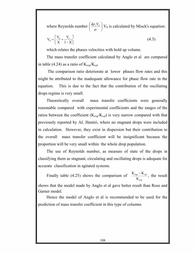
108

where Reynolds number ⎟⎟⎠

⎞⎜⎜⎝

⎛µρ 0Vd c V0 is calculated by Misck's equation:

⎥⎦⎤

⎢⎣⎡

−+=

X1V

XVV cd

0 (4.3)

which relates the phases velocities with hold up volume.

The mass transfer coefficient calculated by Anglo et al are compared

in table (4.24) as a ratio of Kexp/Kcal

The comparison ratio deteriorate at lower phases flow rates and this

might be attributed to the inadequate allowance for phase flow rate in the

equation. This is due to the fact that the contribution of the oscillating

drops regime is very small.

Theoretically overall mass transfer coefficients were generally

reasonable compared with experimental coefficients and the ranges of the

ratios between the coefficient (Kexp/Kcal) is very narrow compared with that

previously reported by AL Hamiri, where no stagnant drops were included

in calculation. However, they exist in dispersion but their contribution to

the overall mass transfer coefficient will be insignificant because the

proportion will be very small within the whole drop population.

The use of Reynolds number, as measure of state of the drops in

classifying them as stagnant, circulating and oscillating drops is adequate for

accurate classification in agitated systems.

Finally table (4.25) shows the comparison of exp

calexp

KKK − , the result

shows that the model made by Anglo et al gave better result than Rose and Garner model.

Hence the model of Anglo et al is recommended to be used for the

prediction of mass transfer coefficient in this type of columns

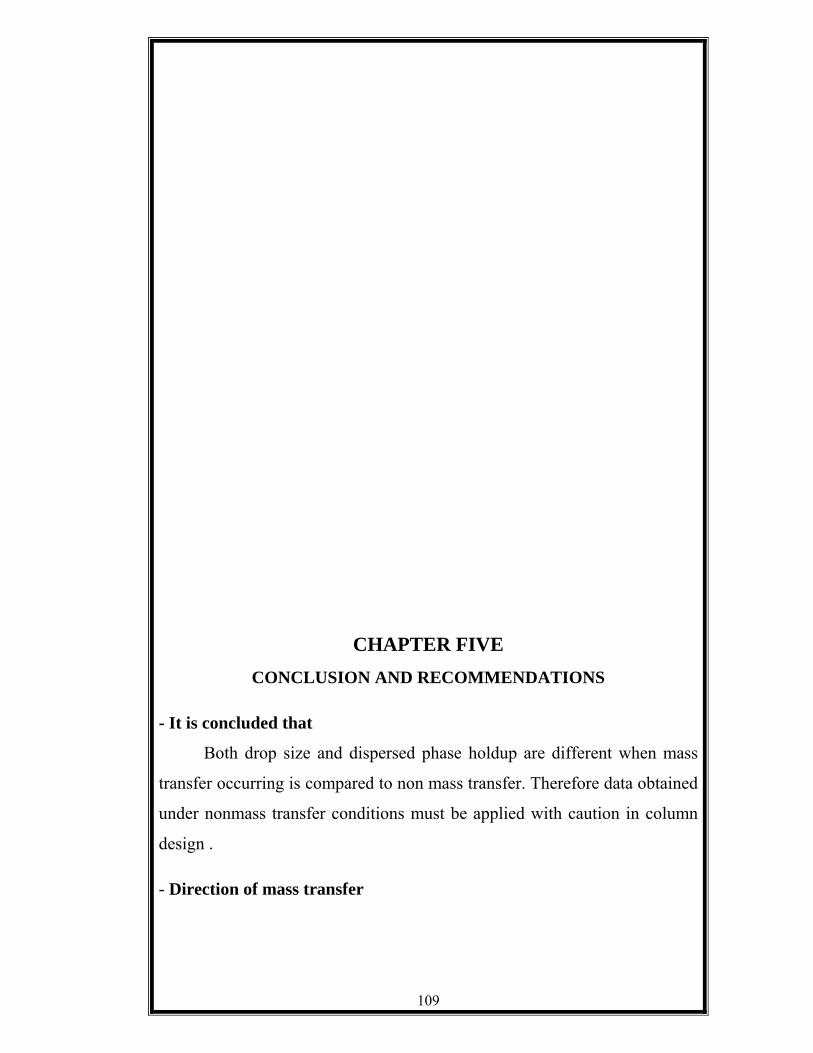
109

CHAPTER FIVE CONCLUSION AND RECOMMENDATIONS

- It is concluded that

Both drop size and dispersed phase holdup are different when mass

transfer occurring is compared to non mass transfer. Therefore data obtained

under nonmass transfer conditions must be applied with caution in column

design .

- Direction of mass transfer

110

With the system studies oil transfer from dispersed to continuous

phase enhanced coalescence with larger drop size and less holdup and vice

versa.

- Experimental overall mass transfer coefficient

The use of the driving force profile along the column to calculate the

mean driving force through Simpson's rule results in a more precise

experimental overall mass transfer coefficient.

- Theoretical over all mass transfer coefficient with drop size

distribution

The use of drop size distribution in the calculation of theoretical

overall mass transfer coefficient gives results that are in agreement with the

experimental coefficients and methods of calculations stated in section 3.7

represent a first step in making such calculations more rigorous without drop

distribution.

The wide diversion in the calculated mass transfer coefficient from

that of the experimental coefficient KEXP confirms that different mass

transfer mechanisms occur simultaneously and that drop size distribution

must be included in calculation process.

-Mass transfer coefficient models

The oscillating drop mass transfer coefficient models of Rose et al

and Garner et al generally give closer results to the experimental coefficient.

5.2 recommendation - The prediction of drop size and dispersed phase under mass transfer

condition are less reliable using the correlation developed for nonmass

transfer conditions.

- To improve the calculation of theoretical overall mass coefficients with

involvement of drop size distribution, more work is needed to find a new

111

basis for classifying the state of drop viz stagnant, circulating, or

oscillating in agitated contactor.

- The effect of the axial, mixing in either phase or both, on the column

performance has long been one of major problem encountered in agitated

extractor operation. Therefore quantitative assessment of this

phenomenon would be very useful.

- The factors that affect mass transfer rate and mass transfer coefficients

were investigated in a sieve tray column, these are the drop size , drop

size distribution, and agitator speed. It was found that the rate of mass

transfer is affected by all these factors. Different models have been used

to predict mass transfer coefficients and model formulated by Angelo et

al was applied and compared with that modeled by Rose and Garner. It is

confirmed that the model formulated by Angelo et al gave less diversion

form the experimental mass transfer coefficient in comparison with that

of Rose and Garner. The result predicted by the above mentioned models

confirmed the superiority of Angelo et al based on this result, Angelo et

al model is recommended to be used for prediction of mass transfer

coefficient in liquid-liquid extraction equipment such as sieve tray

column and other similar equipments.

112

REFERENCES

1. Sherwood, T. K. et al, Ind, Eng. Chem (1939)

2. Jeffreys, G. V. and Ellis, E. M. R (1962).

3. Sawistowski H. and Gotz, G. E. Trans. Ind Chem. Eng (1963).

4. Skelland A. H. P. and Minhas, S. S. A. I971.

5. Heertjes, P. A. and de Wie, L. H. Chem. Eng. (1966).

6. Coulson, J. H. and Skinner, S. J. Chem. Eng, 1951

7. Poporich, A. T. Jervis, R. E. and Trass, O. Chem. Eng. (1969).

8. Heertjes, P. M. and De Wie, L. H. Mass Transfer to Drop, Recent,

Advances, in liquid-liquid Ettraction. Edited by Hanson, C.

Pergamon Press (1971).

9. Rose, P. M. and Kintner, R. C., A. I. Ch, E. Inc. (1966).

10. Angelo, J. b. Lightfoot E. W. and Howard, O. W. A. T. chem. Eng.

Ind. (1966).

11. Forsyth, J. S. et al, Ind Solvent Conf (1974).

12. Garner, F. H. and Tayeban, H. Soc. 1962.

13. Hadamard, C. R. and Rybezynski, A. Acad Sci Paris (1911).

14. Levich. V. Shur. Obstch. Khim. (1949).

15. Garner F. H. and Skelland, A. M. P. Chem. Eng. Sc. (1955).

16. Al-Hassan, T. S. Ph. D. Thesis, University of Aston in Birmingham

U. K (1979).

17. Newman, A. B. Trans. Am. Inst. Chem. Eng (1931).

18. Vermulen, T. Ind. Eng. Chem. (1953).

19. Treybal, R. E. Liquid Extraction, McGraw-Hill new York 2nd

Edition (1963).

20. Kranig, R. and Brink, T. C. App. Sci. Res. (1960).

21. Calderbank P. H. and Korchinski, I. T. O. Chem. Eng. Sci (1956).

22. Handlas, A. E. and Baron, T. A. (1957).

113

23. Skelland, A. H. P. and Wellek, R. H (1964).

24. Johnson, A. I. And Hamleec. A. E. (1960).

25. Olander, D. R. A. I. Ch. E. Ind. (1966).

26. Gunn. R. Jni. Geophys. Res. (1949).

27. Garner, F. H. and Haycock, P. J.. (1959).

28. Johnson, AI and Hamleec, A. E.,. Chem. Eng.Jnl 1960

29. Schroeder, R. R. and Kintner, A. R. C. A. K. chem Ind. (1956).

30. Ellis, W. B., Ph. D. Thesis, University of Maryland U. S. A. (1966).

31. Linton, M. and Sutherland, Chem. Eng. Sci. (1960).

32. Sideman, S. and Shafrai, H. Chem. Eng. (1964).

33. Griffith, R. M. Chem. Eng. Sci. (1960).

34. Garner, F. H. and Suckling, R. D.,. (1968).

35. Rowe, P. N. et al, Trans. Ind. Chem. Engres (1965).

36. Kinard, G. E. Manning, F. S., and, Manning W. P. Chem. Eng.

(1963).

37. Garner, F. H. Foord, A. and Tayeban, M. Appl. Chem., (1959).

38. Mekasut, Molinier. J. and Angelino, 14 Chem. Eng. Sci. (1978).

39. Yamaguchi, M. Watanabe. S and Katayama, T. Ind. Chem. Eng.

Japan (1975).

40. Thorsen, G. et al Chem. Eng. Sci. (1968).

41. Groothuis, H. and Zwiderweg, F. J. Chem. Eng. Sci. (1960).

42. Sawistowski, H. Recent Advances in liquid-liquid extraction edited

by Hanson, C. Pergamon Press W. T. (1971).

43. Al-Hemiri, A. A. A. Ph. D. Thesis University of Aston in

Birmingham U. K. (1976).

44. Arnold, D. R. Ph. D. Thesis University of Aston in Birmingham U.

K. (1974).

45. Mcferrin, A. R. and Davidson, R. R. (1971).

46. Johnson, A. I. And Haieles, A. E. Chem. Jns (1960).

114

47. Licht, W. and Con way, J. B. Int Eng. Chem. (1950).

48. Coulson, J. H. and Skinner, R. E. and Trass, O. Chem., Eng. (1969).

49. Mumford, C. J. Ph. D. Thesis University of Aston in Birmingham

U. K. (1970).

50. Sternling, C. V. and Schriven, L. E. Chem. (1959).

51. Orell, A. and West water, J. W. A. J. Chem. Eng. Sc. (1962).

52. Maroudas, N. G. and Sawistowski, H. Chem. Eng. (1965).

53. Sarkar, S. Ph. D. Thesis University of Aston in Birmingham, U. K.

(1976).

54. Sehrt, B. and Linde, H. P. 3red Berlin (1967).

55. Haydon, D. A. Proc. Soc. (1958).

56. Davies, J. T. “Turbulence Phenomena”. Academic Press New York

(1972).

57. Hoim, A. and Terjesen, S. G. Chem, Eng. (1955).

58. Sieicher, C. A. A. I. (19959).

59. Hartiand, S. and Mechlenburgh, J. C. Chem. Eng. (1966).

60. Harkins, W. D. and Brown, F. E., Ind. (1919).

61. Treybal, R. E. and Howarth, C. B., Ind. Eng. Chem. (1950).

62. Kolmogoroff, A. N. Acad. (1991).

63. Hinze, J. O. I. A. (1955).

64. Ciay, P. H. Proc. Acad. (Amesterdam) (1990).

65. Strand, C. P. Oiney, R. B. and Akermam, G. H.

66. Lawson, G. B. Ph. D. Thesis University (1954), of Manchester

1967.

67. Howarth, W. J. Chem. Eng. (1966).

68. Khandelwal, A. N. Ph . D. Thesis, University of Aston in

Birmingham, U. K. (1978).

69. Todd, D. B. Chem. Eng, (1969).

115

70. Logsdail, D. H. et al. “Recent advancesin Liquid Extraction London

(1971).

71. S.Sajjadi, M. Zerfa, B. W. Brooks, Dynamic behaviour of drops in

oil/water oil dispersions. (2000)

72. Bently, B.J & Leal, L. G. An experimental investigation of drop

deformation and breakup is steady, two- dimensional liner

flows.(1986).

73. Cutter, L. A. flow and turbulence in a stirred tank. (1966).

74. Gopal, E. R. Emulsion science London Academic pree. (1968).

75. Hong, P. O. & Lee, J. M. Unsteady- liquid-liquid dispersions in

agitated vessels. (1983).

76. Al-saadi, A.N.and Jeffreys, G.V. chem..Eng. (1981)

77. Gurashi, A. G. Ph. D.Thesis , University of of Aston in

Birmingham, U. K. (1985).

78. Othmer, D.F. and Tobias, P. E . ind .chem. Eng. (1942)

79. Hand, D. B. Phys.chem .(1930)

80. Rod, V. chem.. Eng. (1966)

116

Appendices

1. Calculation of over all mass transfer coefficients

1.1 The over all experimental mass transfer coefficient

X Y Y* yYY *:∆

4.44 3.23 4.22 0.99

4.04 2.07 3.81 1.82

4.02 2.32 3.82 1.5

3.98 1.41 3.78 2.37

3.88 1.00 3.69 2.61

3.03 0.55 2.88 2.33

1.04 0.05 1.37 1.32

Equilibrium relationship y* = 0.95x

X = Mass fraction of oil in emulsion.

Y = Mass fraction of oil in organic phase.

From table (4.17) d32 = 0.38171

Holdup volume x= 5.5% = 0.055

Effective length of column = 120 cm

Density of emulsion = 0.977 g/cm3

Agitation speed = 200 rpm

Cross sectional area of the column 222

5.706 4

3014.3 4

cmDA =×

==π

The specific interfacial areas 32

6:d

xa

865.03871.0

055.06=

×=a

117

Total interfacial area. vaA .=

27.733345.706120868.0: cmA =××

cmy∆ The mean driving force was estimated by applying Simpson’s rules

as

{ })(2)(4181

53642 yyyyyyyy bottopm ∆+∆+∆+∆+∆+∆+∆=∆

( ) ( ) ( )[ ]063.2

61.25.1233.237.282.1432.199.0181

=

++++++=∆ mY

0211.0100977.0

063.2=

×=∆ mC

Rate of mass transfer

( )57.525.00323.05.706977.0 =×××=

−= outin xxddQN ρ

sec/1059.3 7.733340211.0

57.5 3exp cm

CANK

m−×=

×=

∆⋅=

Theoretical Overall mass Transfer Coefficient

The vertical relative velocity of drop Vo in the column determined by

applying misek’s equation

⎥⎦⎤

⎢⎣⎡

−+=

xV

xVV cd

o 1

02.7035.01

25.0035.0

3.0=

−+=oV cm/sec

The maximum diameter of stagnant drops in the whole drop population

where droplet Reynolds number Re: 10 was found from

10=c

ocs Vdµρ

cmdc 015.0193.9977.0

0104.010=

××

=

The minimum diameter of the Oscillating drop when Re: 200

118

cmdo 303.02.7977.0

0104.0200=

××

=

circulating drops regime

A) Disperesed phase mass transfer coefficient was estimated by

knoning and Brink equation

dcDdKdc

9.17=

dc = from drop size dc :

from diffusion of hexane Dd = 1.1298x10-7 cm2/sec.

sec/106.9242.0

10298.19.17 67

cmKdc−

−

×=××

=

continuous phase mass transfer coefficient was estimated by Garner

42.05.0Re8.1126 ScDc

dcKcc +=

⎟⎠⎞

⎜⎝⎛

××⎟⎠⎞

⎜⎝⎛ ××

+−=×

×−− 77 10119997.0

0102.00102.0

193.9997.02.08.112610119.1242.0ccK

2162645.215. Kcc = -126 + 1.8 (13.41 × 118.15)

seecmKcc /1026.1 3−×=

over all mass transfer coefficient of circulating drops

97.75367.1041661026.1

95.0106.9

1136

0

+=×

+×

= −−cK

61053.964.1049201 −×==ocK

.sec/1053.9 6 cmKoc−×=

24.121)36.10(0102.0

497.0122.08.112610119.1102.0 5.0

7 ×⎟⎠⎞

⎜⎝⎛ ×

+−=×

×=

ccK

)24.12116.10(10812615.911528 ×+−=ccK

Kcc = 2.29 × 10-3 cm/sec

24.1210102.0

45.10947.0104.08.112610119.1109.0 5.0

7 ×⎟⎠⎞

⎜⎝⎛ ××

+−=×

×−

ccK

929901.25 -126+1.8 (10.31 × 121.24) = 2123.97

119

Kcc = 2.28 10-3 cm/sec 42.0

7

5.0

7 10119.1997.00102.0

0102.051.8947.0185.08.1126

10119.1185.0

⎟⎠⎞

⎜⎝⎛

××⎟⎠⎞

⎜⎝⎛ ××

+−=×

×−−

ccK

( )24.12140.128.112689.1653261 ×+−=ccK

= 1.26 + 240.56 = 114.56

Kcc = 1.56 × 10-3

Oscillating drop regime

Dispersed phase mass transfer was firstly estimated by Rose and

Kintner equation 5.0)(45.0 WDK ddo =

⎥⎦

⎤⎢⎣

⎡++

++−=

cd nnnnnn

rbW

ρρ)1()2)(1)(1(6

32

n = 2

( ) 574.0242.1

222.0242.1

225.0225.0

=== odb

cmr 111.02222.0

==

cmdyne /35=δ

⎥⎦

⎤⎢⎣

⎡×+×+++×

=947.02685.0)12()22)(12)(1.2(2

)111.0(5574.035

32W

⎟⎠⎞

⎜⎝⎛

×+××××

947.02685.03431263.14689

42.5

045.434

994.1055.23063.14689 ⎟

⎠⎞

⎜⎝⎛ =

+

W = 295.14

sec/1078.2)14.29510298.1(45.0 35.07 cmKdo−− ×=××=

By ly Angelo

n

EDK

dw

do

⎥⎦⎤

⎢⎣⎡ ++

= 8314

120

11.053.03096.0

434.0−−−

⎥⎦⎤

⎢⎣⎡+⎥

⎦

⎤⎢⎣

⎡⎥⎦

⎤⎢⎣

⎡=

δδρ ocoo

o

do MVVdV

WE

( ) 53.0346.0

35997.0193.9222.0

193.9222.014.295434.0 ⎟⎟

⎠

⎞⎜⎜⎝

⎛ ×⎥⎦⎤

⎢⎣⎡ ×

=−

E

⎟⎠⎞

⎢⎣⎡ ×

−35

193.90102.053.0

⎟⎟⎠

⎞⎜⎜⎝

⎛ ×35

947.0)193.9(222.0)405.0(434.03

017.1)91.4)(406.0(434.0 +

912.143.0406.0434.0 ×××

0.145

E = 0.145

π

⎟⎠⎞

⎜⎝⎛ ++

=

2

8314 EiwD

Ko

do

π

27 )145.0(8345)01(14.29510298.14 ++×××

=

−

AngleocmKdo .sec/1049.7 3−×=

The over all mass transfer coefficient

ooVK11 = Oscillating drops

0.

1

cdooo K

mK

K +=

Continuos phase mass transfer coefficient

ocK . = was estimate by Garner correlation

7.00. Re0085.050 scD

dK

c

oc +=

7.0

770.

10119.1977.00102.0

0102.0977.0193.9222.00085.050

10119.1222.0

⎟⎠⎞

⎜⎝⎛

×××⎟

⎠⎞

⎜⎝⎛ ××

+=×

×−−

cK

1983914.21 Kco

121

( )97.296948.1990085.050 ×+=

21.1983914 Kco 76.94

Kco = 2.56 × 10-3 cm/sec

codo KKK95.011

0.0

+=

350.0 1078.2

11088.3

95.01−− ×

+×

=K

71.35954.244841

.

+=ooK

Ko.o = 4.03 × 10-5 cm/sec by Rose and Kitner by Anglo

⎥⎥⎥⎥

⎦

⎤

⎢⎢⎢⎢

⎣

⎡

+=

DcDdm

KK odoo

1

1..

⎥⎥⎥⎥

⎦

⎤

⎢⎢⎢⎢

⎣

⎡

××

+

×=−

−

7

7

3.

10119.110298.195.01

11044.7ooK

33 1031.3954.111049.7 −− ×=⎥⎦

⎤⎢⎣⎡× cm/sec.

Oscillating drop regime Dis phase Kdo by Rose and Kintner

( ) 5.045.0 WDK odo =

⎥⎦

⎤⎢⎣

⎡++

++−=

cd nnnnnn

rbW

ρρδ

)1()2)(1)(1(

32

n = 2

( ) 589.0242.1

240.0242.1

225.0225.00 ===

db

12.02240.0

2=== odr

35=δ

122

⎥⎦

⎤⎢⎣

⎡++

++−×=

cn nW

ρρ)12()22)(12)(1.2(2

)12.0(589.035

32

( )497.02685.03

431270.11828×+××××

93.549.4

24994.1055.2

24==

+

W = 264.85

Run N2 sec/1093.3)85.26910298.1(45.0 35.07 cmKdo−− ×=××=

Run N3 r = 0.212 b. ( ) 568.0242.1

21.0 225.0

=

2)93.5(3

2 odwrbW ===δ

61.31493.5212.0(1568.935

=×−×

( ) ( ) 5.07 )61.31410298.1(48.045.0 ×××= −dwdo DK

2.87 × 10-3 cm/sec. 5.0)(45.0 WDK ddo =

5.07 )10298.1(45.0 WKdo ××= −

93.532 ×=

rbW δ

( ) 564.0242.1205.0

292.10 ===

db

70.32993.5)1085.0(

564.0352 =×

×=W

sec/1094.2)7.32910298.1(45.0 35.07 cmKdo−− ×=××=

5.07 )10298.1(45.0 WKdo−×=

93.532 ×=

rbW δ

561.0242.1

)200.0(242.1

225.0225.00 ===

db

1.022.0

22 === odW

123

1963593.5)1.0(561.0353

2 =××

=W

12.14019635 ==W

.sec/1092.1)12.190298.1(45.0 35.0 cmKdo−×=×=

Kdo by Angelo

π

⎥⎦⎤

⎢⎣⎡ ++

=Ee

WDK ddo831

4

5353.0046

434.0−−−

⎥⎦⎤

⎢⎣⎡

⎥⎦⎤

⎢⎣⎡

⎥⎦

⎤⎢⎣

⎡=

δδρ ocoo

o

o MVVdV

WdE

⎥⎦⎤

⎢⎣⎡ ××

⎥⎦⎤

⎢⎣⎡ ×

=−

35997.0512.829.0

51.824.089.264934.0

46.0

E

11.0

3551.80102.0 −

⎟⎠⎞

⎜⎝⎛ ×

384.1935.1515.4935.1434.0 =×××=

155.093.1467.0397.0434.0 =×××

π

27 )155.0(

83155.0184.26410298.14 ⎟

⎠⎞

⎜⎝⎛ ++×××

=

−

doK

7.1410-3 cm/sec.

⎟⎟⎟⎟

⎠

⎞

⎜⎜⎜⎜

⎝

⎛ ++=

π

EEWDK odo

831

.4

11.053.0346.0

434.0−−−

⎥⎦⎤

⎢⎣⎡×⎥

⎦

⎤⎢⎣

⎡×⎥

⎦

⎤⎢⎣

⎡=

δδρ ocoo

o

o MVVdV

WdE

53.0346.0

35997.0)62.9(212.0

62.9212.061.314434.0

−−

⎥⎦

⎤⎢⎣

⎡ ×××⎥⎦

⎤⎢⎣⎡ ×

=E

4.0

3562.90102.0 −

⎟⎠⎞

⎜⎝⎛ ×

( ) 140.0908.141.00413434.0 =××=E

124

( )

π

⎟⎠⎞

⎜⎝⎛ ++×××

=

− 27 14.08314.0161.31410298.14

doK

.sec/1072.7 3cmKdo−×=

199.0897.1386.0628.0(434.0 =××=doK

( )

π

⎟⎠⎞

⎜⎝⎛ ++×××

=

− 27 199.083199.0112.14010298.14

doK

5.30×10-8 cm/sec. 53.0346.0

35997.0)36.10(197.0

36.10197.099.347434.0

−−

⎥⎦

⎤⎢⎣

⎡ ×××⎥⎦

⎤⎢⎣⎡ ×

=doK

4.0

3536.100102.0 −

⎟⎠⎞

⎜⎝⎛ ×

Kdo = 0.434 (0.4191037 × 1.893) = 0.130

( )

π

⎟⎠⎞

⎜⎝⎛ ++×××

=

− 27 13.083199.0112.34710298.14

doK

.sec/1007.8 3cmKdo−×=

b) Continuous phase mass transfer coefficient was estimated

by Garner et al correlation

7.0Re0085.050 scD

dK

c

oco +=

⎟⎠⎞

⎜⎝⎛ ××

+=××

− 0102.0997.051.824.00085.050

10119.124.0

7coK

7.0

710119.1977.00102.0

⎟⎠⎞

⎜⎝⎛

×× −

)97.296963.199(85.5011.2149772 ×+= oooKco

.sec/1037.2 3cmKco−×

7.0

710119.1997.00102.0

0102.0797.06.9212.08085.050

119.1⎟⎠⎞

⎜⎝⎛

××⎟⎠⎞

⎜⎝⎛ ××

+=cooKK

)97.296914.199(0085.0507.1894598 ×+=coK

125

.sec/1068.2 3cmKco−×=

⎟⎠⎞

⎜⎝⎛

××⎟⎠⎞

⎜⎝⎛ ××

+=× −− 77 10119.1977.0

0102.00102.0

997.094.9205.00088.05010119.1

205.0coK

)97.296418.199(0085.05085.1831992 ×+=

.sec/1077.2 3 cmKco−×=

710119.1197.0

−×=coK

97.29640102.0

997.036.10197.00085.05045.1760500 ×⎟⎠⎞

⎜⎝⎛ ××

+=coK

97.296949.99.10085.050 ××+

.sec/1089.2 3 cmKco−×=

c) The over all mass transfer coefficient oscillating drops

codooo Km

KK+=

11

337 104927.222.1900560

1037.295.0

1071411 −

−− ×+=×

+×

=ooK

.sec/1014.7 7. cmK oo

−×=

.sec/1007.2536.1291065.2

95.01072.7

11 333 cm

Koo

−−− ×+=

×+

×=

Ko.o by Angelo

⎥⎥⎥⎥

⎦

⎤

⎢⎢⎢⎢

⎣

⎡

+=

DcDdm

KK dooo

1

1.

3

7

7

3.. 1053.3

10119.110298.1

195.01

11014.7 −

−

−

− ×=

⎥⎥⎥⎥

⎦

⎤

⎢⎢⎢⎢

⎣

⎡

××+

×=ooK

126

The theoretical over mass transfer coefficient for the whole drop

population by Rose and Kintner and Garner

)1(. VKVKK oooccal −+=

.sec/1011.37.01003.43.01053.9 556 cmKcal−−− ×=××+××=

127

Chemical and physical properties of n.hexane

density 0.658 g/cm3 Molecular weight 86 Boiling point 68o c Freezing point – 95o c Flash point -22o c Viscosity 0.294 cps Surface tension 18.48 dyn/cm

Chemical and physical properties of Emulsion

1. Density 0.977g\ cm3 2. Viscosity 0.324 cps

128

equilibrium relationship

0

0.01

0.02

0.03

0.04

0.05

0.06

0.07

0 0.01 0.02 0.03 0.04 0.05 0.06

mass fraction of oil in imulsion

mas

s fr

ctio

n of

oil

in o

rgan

ic p

hase

equilibrium relationship

0

0.01

0.02

0.03

0.04

0.05

0.06

0.07

0 0.01 0.02 0.03 0.04 0.05 0.06

mass fraction of oil in imulsion

mas

s fr

ctio

n of

oil

in o

rgan

ic p

hase

UNIVERSITY OF KHARTOUM - COREUNIVERSITY OF KHARTOUM FACULTY OF ENGINEERING & ARCHITECTURE DEPARTMENT...

Documents

Transcript of UNIVERSITY OF KHARTOUM - COREUNIVERSITY OF KHARTOUM FACULTY OF ENGINEERING & ARCHITECTURE DEPARTMENT...