UNIVERSITY OF HAWAl'1 LIBRARY

EFFECT OF PARTICLE SHAPE ON GRAIN SIZE, HYDRAULIC, ANDTRANSPORTCHARACTEmSTICS OF CALCAREOUS SAND

A DISSERTATION SUBMITTED TO THE GRADUATE DIVISION OF THEUNIVERSITY OF HAWAI'I IN PARTIAL FULFILLMENT OF THE

REQUIREMENTS FOR THE DEGREE OF

DOCTOR OF PHILOSOPHY

IN

OCEAN ENGINEEmNG

AUGUST 2003

By

David A. Smith

Dissertation Committee:

Kwok Fai Cheung, ChairpersonHorst G. Brandes

Charles H. FletcherHans-Jiirgen KrockEugene R. Pawlak

© Copyright 2003

by

David A. Smith

iii

ACKNOWLEDGEMENTS

The following people are acknowledged for their assistance with this project:

• Dr. Kwok Fai Cheung, advisor and principal investigator on this project, who

provided excellent guidance throughout the research, and without whom this project

never would have materialized;

• My parents, Stewart and Vyta Smith, for their years of support;

• Dr. Hans Krock and Mr. Roland Kanno, for assistance in the work performed at

Look Laboratory;

• Dr. A.N. Papanicolaou and the staff and students of the Albrook Hydraulic

Laboratory at Washington State University, for their guidance and assistance in

performing the flume experiments;

• Mr. Ray Rojas, Dr. Nick Dodd, Dr. Amal Phadke, Dr. Ron Bozak, Mr. Jeff

McKeown, and the lifeguards at Ehukai Beach Park for their help collecting sand;

• Dr. Charles Fletcher, Dr. Ralph Moberly, Mr. Marc Ericksen, and Mr. Jim Barry, for

critical reviews ofjoumal article manuscripts based on this dissertation;

• Drs. Horst Brandes and Eugene Pawlak and the other committee members for their

comments on this dissertation;

• Ms. Edith Katada, for many aspects, including always knowing which forms go

where;

• Miss Winnie Law, for her assistance with the presentation;

• and the many others with whom I have crossed paths, for enriching my life and

expanding my knowledge of ocean engineering and the world.

This project was funded by the University of Hawaii Sea Grant College Program under

Institutional Grant No. NA36RG0507.

IV

ABSTRACT

This study examines the grain size, fall velocity, initiation of motion, and sediment

transport rates of calcareous sand collected on Oahu, Hawaii. These characteristics are

unique to calcareous sand owing to the irregular shape of the particles and are distinct

from those of siliceous sand, which have been studied extensively with well-documented

results. Through a series of laboratory experiments and data analyses, this study provides

a comprehensive data set of calcareous sand characteristics and quantifies their

dependence on particle shape.

Sand samples were selected from the swash zones of Oahu beaches. Sieve and

settling techniques separate the samples into groups by sieve size and fall velocity,

respectively. Individual grain properties such as shape factor, intermediate dimension,

fall velocity, and nominal and equivalent diameters for 998 grains within those groups are

presented. Evaluation of the grain size data by sieve and settling groups provides

empirical relationships between the median sieve size of the sand samples and the

corresponding nominal and equivalent diameters. The fall velocity and drag coefficient

expressed respectively as functions of nominal diameter and Reynolds number show

strong correlation over a wide range of shape factors. Analysis of the data by flow regime

shows that particle shape has stronger influence on the settling characteristics when

unstable wakes develop behind the grains.

These findings are used to interpret the initiation of motion of four natural and five

sieved calcareous sand samples in unidirectional flow. Flume experiments provide the

sediment transport rate as a function of bed shear stress up to bed-form development.

Reference-based criteria are supplemented by visual observations to determine the critical

shear stress. The results are compared with published data for rounded and irregular

particles in terms of the median sieve size and median nominal and equivalent diameters

over Reynolds number. The critical shear stresses of the irregular particles, in comparison

v

with data for rounded particles, are higher in the hydraulically smooth regime and lower

in the rough turbulent regime.

Finally, the transport of calcareous sand in unidirectional flow and its prediction

through existing sediment transport models are examined. Flume experiments provide 70

sets of sediment transport data and the results are compared with direct predictions from

five published sediment transport models developed for siliceous particles. Corrections

for the grain size and hydraulic characteristics of calcareous sand developed in this study

are applied and the results are compared with the direct calculations. The comparisons

show that one of the models gives good results before calcareous sand corrections are

considered and another responds well when the corrections are applied. This analysis

provides guidelines to the application of existing sediment transport models to calcareous

beaches and the gathered data lays a foundation for future model development.

VI

TABLE OF CONTENTS

Acknowledgements iv

Abstract v

List of Tables ix

List of Figures ." x

1. INTRODUCTION 1

1.1 Calcareous Sand 1

1.2 Grain Size and Hydraulic Characteristics 2

1.3 Objectives and Approach " 5

2. PHYSICAL GRAIN SIZE CHARACTERISTICS 7

2.1 Sand Samples 7

2.2 Measurements of Grain Properties 8

2.3 Sand Density 9

2.4 Particle Shape and Characteristic Dimensions 11

3. HYDRAULIC GRAIN CHARACTERISTICS 14

3.1 Settling Tube Analysis 14

3.2 Settling Mode and Sensitivity 14

3.3 Fall Velocity and Equivalent Diameter 16

3.4 Drag Coefficient 17

3.5 Shape Effect versus Flow Regime 19

4. MEDIAN GRAIN SIZE 21

4.1 Settling Techniques 21

4.2 Sieving versus Settling Techniques 22

4.3 Median Grain Size Parameters 23

5. INITIATION OF MOTION 27

5.1 Sand Samples 27

vii

5.2 Test Setup and Preparation 28

5.3 Test Procedure 29

5.4 Characteristic Grain Diameters 30

5.5 Bed-load Transport 32

5.6 Definitions of Initiation of Motion 33

5.7 Initiation of Motion 35

6. TRANSPORT RATES 38

6.1 Test Setup and Procedure 38

6.2 Transport Models 40

6.2.1 Engelund-Hansen (1967) 40

6.2.2 Ackers and White (1973) .41

6.2.3 Yang (1973, 1979) 43

6.2.4 van Rijn (1984c) 44

6.3 Model Implementation 45

6.4 Corrections for Calcareous Sand 46

6.5 Comparison of Transport Rates 48

7. CONCLUSIONS AND RECOMMENDATIONS 52

Appendix A. Plane-bed Transport Data 91

Appendix B. Bed-load and Suspended-load Transport Data 93

Literature Cited 94

VIll

LIST OF TABLES

Table Page

2-1. Sand Densities for Natural Samples 56

2-2. Sand Densities for Sieved Samples 57

3-1. Results from Fall Velocity Sensitivity Test. 58

4-1. Median Diameters Determined from Sieve and Settling Analyses 59

5-1. Grain Size Characteristics of Sand Samples 60

6-1. Hydraulic Characteristics of Sand Samples 60

6-2. Model Error and Scatter for Uncorrected Results at Various Transport Stages 61

6-3. Model Error and Scatter for Corrected Results at Various Transport Stages 61

IX

LIST OF FIGURES

Figure

I-I. Photographs of natural calcareous sand samples. (a) Kailua Beach sand: D so =0.20 mm. (b) Waimanalo Beach sand: Dso = 0.29 mm. (c) Puuiki Beach sand:Dso =0.67 mm. (d) Ehukai Beach sand: Dso=0.76 mm 62

2-1. Location map of sand sampling 63

2-2. Calcareous sand density as a function of median nominal diameter. 0: naturalsand; e: sorted sand 64

2-3. Particle shape classification by D/D, and D,IDi 65

2-4. Relationships between characteristic grain sizes. (a) Intermediate dimension andsieve size. --, linear size relationships. (b) Nominal diameter andintermediate dimension. --, linear trendline 66

2-5. Distributions of shape factor. (a) Shape factor versus nominal diameter. --,linear trendline. (b) Probability density. --, normal distribution fitted to data... 67

3-1. Fall velocity of calcareous sand as a function of nominal diameter and shapefactor. Present data: 0, 0.15 < Fs < 0.25; C, 0.25 < Fs < 0.35; 0, 0.45 < Fs <0.55; 6, 0.65 < F s < 0.75. --, regressed curves. - -, Baba and Komar(1981) 68

3-2. Relationship between nominal diameter and equivalent diameter. Present data:0, 0.15 < Fs < 0.25; 0, 0.25 < Fs < 0.35; 0, 0.45 < Fs < 0.55; 6, 0.65 < Fs <0.75. --, regressed curves 69

3-3. Drag coefficient of calcareous sand as a function of Reynolds number and shapefactor. Present data: 0,0.15 < Fs < 0.25; 0,0.25 < Fs < 0.35; 0, 0.45 < Fs <0.55; 6, 0.65 < Fs < 0.75. --, regressed curves. - -, Baba and Komar(1981) 70

3-4. Ratio of measured fall velocity to fall velocity of a sphere as a function of shapefactor. 0, stable regime; 6, transitional regime; 0, unstable regime. --,regressed curves. - -, Baba and Komar (1981) 71

3-5. Ratio of measured drag coefficient to drag coefficient of a sphere as a functionof shape factor. 0, stable regime; 6, transitional regime; c, unstable regime.--, regressed curves 72

4-1. Schematic of long settling tube experiment. 73

x

4-2. Cumulative grains size distribution for Ehukai Beach in terms of sieve size 74

4-3. Cumulative grains size distribution for Ehukai Beach in terms of nominaldiameter. (a) Sieve analysis. (b) Settling analysis. --, median curve 75

4-4. Cumulative grain size distribution for Ehukai Beach in terms of equivalentdiameter. (a) Sieve analysis. (b) Settling analysis. --, median curve 76

4-5. Median nominal diameter versus median sieve size. (a) Sieve analysis. (b)Settling analysis. --, linear trend1ine 77

4-6. Median equivalent diameter versus median sieve size. (a) Sieve analysis. (b)Settling analysis. --, linear trend1ine 78

4-7. Empirical relationships of median grain sizes. (a) Median nominal diameter andmedian sieve size. (b) Median equivalent diameter and median sieve size. --,linear trendline; - - - -, power curve 79

5-1. Schematic of flume experiment for initiation of motion tests 80

5-2. Shear stress versus bed-load transport rate of calcareous sand. (a) Natural sandsamples. x, scuffed bed; +, packed bed for Dn '" 0.90 mm. (b) Sorted sandsamples. --, regressed curves; *, point of maximum curvature 81

5-3. Initiation of motion diagram in terms of median equivalent diameter. Presentstudy: ., natural calcareous sand; ., sieved calcareous sand. Paphitis et al.(2002): 0, mussel particles; +, cockle particles. Prager et al. (J 996): x,calcareous sand. Brownlie (J 981): --, Shields curve 82

5-4. Initiation of motion diagram in terms of median nominal diameter. Presentstudy: ., natural calcareous sand; ., sieved calcareous sand. Prager et al.(1996): x, calcareous sand. Magalhaes and Chau (1983): c, shale particles.Brownlie (1981): --, Shields curve 83

5-5. Initiation of motion diagram in terms of median sieve diameter. Present study:., natural calcareous sand; ., sieved calcareous sand. Paphitis et al. (2002): 0,

mussel particles; +, cockle particles. Prager et al. (1996): x, calcareous sand.Magalhaes and Chau (1983): c, shale particles. Brownlie (1981): --, Shieldscurve 84

6-1. Schematic of flume experiment for bed-form and suspended transport tests 85

6-2. Calculated versus measured sediment transport rates using Engelund-Hansen(1967) model. 0, ., plane-bed transport stage; 0, ., bed-form transport stage; t:>,

&, suspended transport stage (0, 0, t:>: uncorrected; ., ., &: corrected). --,perfect agreement; - - -, factor of 2 difference; ......., factor of 10 difference........ 86

xi

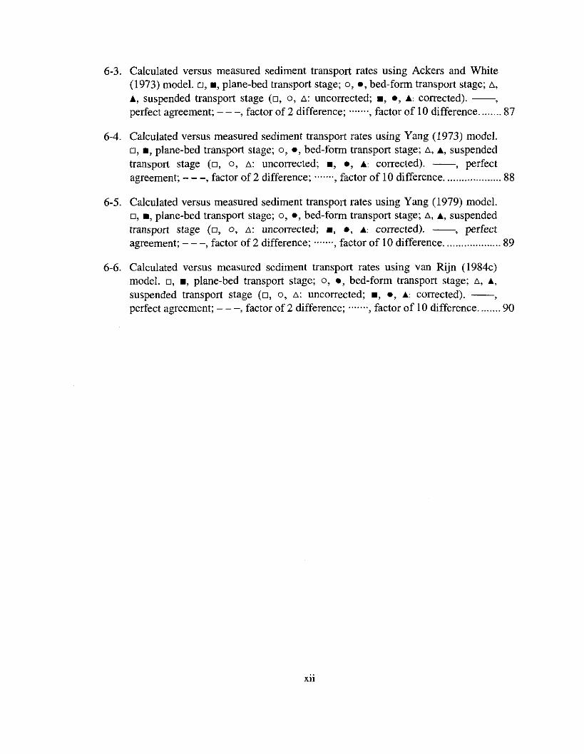
6-3. Calculated versus measured sediment transport rates using Ackers and White(1973) model. 0, ., plane-bed transport stage; 0, ., bed-form transport stage; 6.,

A, suspended transport stage (0, 0, 6.: uncorrected; ., ., A: corrected). --,perfect agreement; - - -, factor of 2 difference; , factor of 10 difference 87

6-4. Calculated versus measured sediment transport rates using Yang (1973) model.0, ., plane-bed transport stage; 0, ., bed-form transport stage; 6., A, suspendedtransport stage (0, 0, 6.: uncorrected; ., ., A: corrected). --, perfectagreement; - - -, factor of 2 difference; , factor of 10 difference 88

6-5. Calculated versus measured sediment transport rates using Yang (1979) model.0, ., plane-bed transport stage; 0, ., bed-form transport stage; 6., A, suspendedtransport stage (0, 0, 6.: uncorrected; ., ., A: corrected). --, perfectagreement; - - -, factor of 2 difference; , factor of 10 difference 89

6-6. Calculated versus measured sediment transport rates using van Rijn (I984c)model. 0, ., plane-bed transport stage; 0, ., bed-form transport stage; 6., A,

suspended transport stage (0, 0, 6.: uncorrected; ., ., A: corrected). --,perfect agreement; - - -, factor of 2 difference; , factor of 10 difference 90

Xli

1. INTRODUCTION

1.1 Calcareous Sand

Tropical island beaches are composed of calcareous sand of marine ongm,

specifically fragments of such reef-dwelling organisms as coral, coralline algae,

foraminifera, and molluscs. The grains of these species have a wide variety of shapes

associated with their biological origins in contrast to the rounded, uniform siliceous sand.

Moberly and Chamberlain (1964) and Zapka (1984) reported the physical properties

related to the chemical composition, hardness, density, and shape of calcareous sand. Dai

(1997) showed that the particle shape plays an important role in the engineering

properties of calcareous sand.

Figure 1-1 shows photos of calcareous sand particles from four Oahu beaches. The

coarsest two sand samples were obtained from Ehukai Beach and Puuiki Beach, both on

Oahu's North Shore, while the finer two sand samples are from Waimanalo Beach and

Kailua Beach on the windward shore of Oahu. The particles in the figure have a variety

of shapes, including rounded, rod-shaped, and flat. Smooth and sharp-edged particles are

also seen, as well as non-symmetric particles. Moberly (1963) reported on the coastal

geology of Hawaiian beaches and found that the distribution of components within the

beach sand is site specific.

The various components of calcareous sand produce particle shapes that are

significantly different from siliceous sand. Particle shape affects grain size measurements

as well as the hydraulic properties. Sieve analysis produces biased size distributions as

the particle shape deviates from spherical, causing an error in the measurement of the

mass of the particle. The drag on an irregular particle is increased relative to a sphere, as

particle shape modifies the boundary layer around the grain, and affects the motion

characteristics and transport mechanisms.

1

The hydraulic properties such as fall velocity, critical shear stress, and transport rates

of siliceous sand have been studied extensively, and yet similar information for

calcareous sand is limited. Previous studies have suggested the importance of particle

shape on the physical and hydraulic properties of sediment, but its impact on the transport

rate is not well understood.

1.2 Grain Size and Hydraulic Characteristics

The choice of a characteristic sand size becomes important when the particle shape

deviates from spherical. The nominal and equivalent diameters, which are the diameters

of a sphere having respectively the same volume and settling velocity as the irregular

particle, are commonly used. Sieve analysis, however, becomes biased at determining

these properties as particle shape deviates from spherical. Despite this limitation, sieve

analysis remains the most common technique to determine grain size properties for

calcareous sand (e.g., Frith, 1983; Sagga, 1992; Lipp, 1995; and Harney et aI., 2000). A

consistent description of the grain size characteristics is necessary to compare the results

with other data sets. Relationships that can be applied directly to sieve analysis results to

infer the nominal and equivalent diameters of calcareous sand are highly desirable.

Maiklem (1968) and Braithwaite (1973) were among the first to determine the size

distributions of calcareous sand in terms of equivalent diameter by settling analysis. This

approach sorts sediment hydraulically in a settling tube and the results encompass the

effects of size, shape, and density of the particles. Sanford and Swift (1971), Komar and

Cui (1984), and Lund-Hansen and Oehmig (1992) showed that sieve and settling

techniques yield similar grain size distributions for silicate sand with uniform density and

shape. However, Kench and McLean (1996, 1997) compared sieve and settling

techniques for calcareous sediment and showed that the grain size distribution in terms of

equivalent diameter obtained from settling analysis is significantly different from the size

2

distribution fowld directly by sieve analysis. De Lange et al. (1997) showed that sieve

and settling analyses do not produce the same textural parameters for sand samples

composed of mixtures of quartz, feldspar, and volcanic glass. The discrepancy of the two

techniques is expected because sieve size and equivalent diameter deviate from each

other as particle shape deviates from spherical.

Particle shape also affects fall velocity. Studies have been undertaken to quantify the

fall velocity of non-spherical particles in terms of shape factor. Shultz et al. (1954)

investigated the influence of particle shape on the fall velocity of river gravel and the

results were re-analyzed by Swamee and Ojha (1991). Alger and Simons (1968) obtained

fall velocities and drag coefficients for ten ellipsoidal pebbles settling through eight

different fluids. Komar and Reimers (1978) investigated the settling characteristics of 51

smooth, symmetric pebbles in glycerine and presented relationships for the fall velocity

and drag coefficient by interpolation with Alger and Simons' data. Baba and Komar

(1981) later examined the settling characteristics of70 natural quartz grains and obtained

lower fall velocities in comparison to those of smooth, symmetric pebbles.

The effect of shape on grain size and settling properties provides insight into the

initiation of motion ofcalcareous sand. Shields (1936) pioneered the study of initiation of

motion and his dimensional analysis results in a relationship of dimensionless shear stress

in terms of Reynolds number. Many subsequent studies with rounded, uniform particles

confirmed Shields' data and the results were compiled in Miller et al. (1977) and

Buffington and Montgomery (1997). There is, however, only scattered data pertaining to

irregular particles. Magalhaes and Chau (1983) undertook flume studies on initiation of

motion for shale particles, while Prager et al. (1996) and Paphitis et al. (2002) examined

calcareous sand and shell fragments, respectively. Each of these studies covers a limited

range of Reynolds numbers and produces results noticeably different from Shields'

findings. The discrepancy is primarily due to particle shape, but other factors such as

3

surface texture and sharp edges may also playa role. Motion initiation characteristics for

calcareous sand are necessary for estimating sediment transport rates.

Grain size, fall velocity, and critical shear stress are typical input parameters for

sediment transport models. Chang (1988), van Rijn (1993), Yang (1996), and Yang and

Huang (2001) provide comprehensive reviews of numerous sediment transport models

and discuss their applications in coastal and river environments. The applicability of

these equations for use with calcareous sand is unclear. The initiation of motion of

irregularly shaped and calcareous particles has been studied (e.g., Mantz, 1977; and

Magalhaes and Chau, 1983) and specifically for calcareous particles (e.g., Prager et al.,

1996), and Kench and McLean (1996) used settling fractions to interpret calcareous

depositions, but there are few published studies on the transport rates of calcareous sand.

Based on the premise that the grain size distribution and properties determined from

settling analysis correctly reflect the hydraulic characteristics of the sand sample, Kench

and McLean (1997) examined the interpretative use of the results for sediment transport

models developed for silicate sand. While the equivalent diameter determined from

settling analysis better represents calcareous sediment in suspension, motion initiation

and bed-load transport are more appropriately described by the nominal diameter, which

relates to the weight of the particles only. Dai (1997) and Miller (1998) examined the use

of these sediment size parameters to predict the response of tropical island beaches to

waves and currents.

The interpretive use of existing transport models depends on accurate input of the

grain size characteristics, fall velocity, and motion initiation, which are still not well

defined for calcareous sand. Such an approach provides convenient predictions of

calcareous sand transport rates, but its validity is unproven. There is a consensus within

the coastal engineering communities in Hawaii and other tropical regions that existing

sediment transport models need to be re-examined for calcareous sand conditions.

4

1.3 Objectives and Approach

The present study compiles and evaluates the umque physical and hydraulic

characteristics of calcareous sand on Oahu, Hawaii. The specific objectives of the study

are to:

1. Examine grain shape and size characteristics;

2. Develop relationships for fall velocity and drag coefficient as a function of grain size

and shape;

3. Produce relationships to compare median sand properties found by sieve and settling

analyses;

4. Determine the critical shear stress for initiation of motion; and

5. Measure sediment transport rates and compare with published models for calcareous

sand collected on Oahu.

This study is directed toward the coastal erosion problem faced by Hawaii and other

tropical environments. Though a series of measurements and analyses, a better

understanding of the unique physical and hydraulic characteristics of calcareous sand is

provided and the interpretive use of existing sediment transport models with the

calcareous sand properties as input is investigated.

The applicability of sieve analysis for determining grain size characteristics of

calcareous sand is first studied. Relationships amongst sieve size, nominal diameter,

intermediate dimension, and shape factor are developed. The settling characteristics of

calcareous grains are then investigated to provide a more comprehensive description of

the particle shape effect on fall velocity and drag coefficient over the applicable size

range. The data is analyzed by flow regime to show the effect of particle shape on the

settling characteristics as a function of the wake that develops behind the grains. Empirical

relationships between the various grain size definitions and between the sieve and settling

results are determined using the calcareous sand samples. These relationships allow

5

continued use of sieve analysis as the standard method for characterizing sediment and

provide correction factors so that data from sieve analysis can be properly interpreted and

used in sediment transport models.

A series of flume experiments provides measurements of transport rates at various

transport stages. The experiments utilize natural sand samples and sieved fractions to

show the effects of classifying non-uniform sediment according to a single characteristic

diameter. Initiation of motion of calcareous sand is investigated with special attention to

the various particle size characterizations. The study culminates with an independent

assessment of five commonly used sediment transport models for calcareous sand

conditions. The results are used to provide guidelines for the selection and interpretative

use of existing transport models for calcareous sand conditions.

6

2. PHYSICAL GRAIN SIZE CHARACTERISTICS

2.1 Sand Samples

Oahu beaches are composed mainly of calcareous sand. Samples of beach sand were

obtained from the swash zone at numerous Oahu beaches, the locations of which are

shown in Figure 2-1. The selected sites provide a balanced representation of the sediment

sizes commonly found on tropical island beaches. Most of these sites were selected

because of their potential to supply large quantities of good quality samples for the

subsequent transport tests.

The north and west shores of Oahu have seasonally high-energy beaches. Swell from

North Pacific storms reach these shores in the winter, when surf regularly exceeds 3 ffi.

These beaches can experience rapid sediment loss during periods of high surf, but recover

during the gentler sununer season, when the waves are longer and less steep. The east and

south shore beaches are generally low to medium-energy beaches exposed to the trade­

wind waves, with some reaction to north or south swell. High-energy beach sediment

tends to be coarser and the beach slope steeper than lower energy beaches (Gerritsen,

1978).

While the exact composition of the sand is site specific, the main constituents of

beach sand around Oahu are foraminifera, coralline algae, and mollusc shells, with lesser

amounts of coral, echinoids, and Halimeda (Moberly, 1963). A limited amount of

volcanic rock fragments is also found in the sand. The species that constitute the sand

have unique particle shapes. Foraminifera are the most spherical, while sand grains

derived from coralline algae have a variety of shapes. Fragments of mollusc shells are

generally blade and disk-shaped. The spines of echinoids tend to be rod-shaped and

Halimeda are disk-shaped. Kench and McLean (1997) reported that sand grains of the

coral genus Pocillopora are also rod-shaped.

7

The mixture of different species in natural beach sand gives rise to a wide range of

particle shapes. Classification of calcareous sand by biological composition can provide a

qualitative description of the particle shape, but falls short of providing quantitative data

that can characterize the sediment as a whole.

2.2 Measurements of Grain Properties

The sand samples were carefully cleansed and prepared prior to the analyses. Each

sample was rinsed with fresh water, dried in a 95°C oven, and divided into sub-samples.

Dry sieve analysis was performed using a series of 15 eight-inch sieves ranging in mesh

size from 0.063 mrn to 4.76 mrn. Each sample of approximately 600 to 1000 grams was

shaken for 15 minutes and each sieve fraction was weighed and saved in a separate bag.

Grain size distributions by weight were determined graphically. The median diameter,

D50, and sorting parameter, cr, of each sample are determined. Sorting is defined as

(2-1)

where Dl6 and D84 are the 16th and 84th percentiles of the grain size according to sieve

analysis. Twelve grains were chosen at random from each sieve fraction for subsequent

analyses to determine their dimensions and fall velocities.

The individual grains obtained from the sieve analysis were analyzed for shape factor,

nominal diameter, and intermediate dimension. Grain dimensions in the three principal

orthogonal directions were measured using a dissecting microscope with 10.4 to 72 times

magnification and readability of 0.017 mrn. The range of dimensions measurable is 0.017

mrn to 13.3 mrn, which covers the particle sizes considered in this study. The particle

shape is described using the Corey shape factor defined as

(2-2)

8

where D" Di, and D{ are the respective short, intermediate, and long mutually orthogonal

dimensions of the grain (Dyer, 1986). This shape factor measures the sphericity of the

particle and has a maximum value of one for spheres and decreases toward zero as the

particle shape deviates from being spherical. The particle shape can be described more

precisely by the morphometry index of Sneed and Folk (1958), differentiating spheres,

rods, and disks in a triangular diagram (e.g., Verrecchia et aI., 1997), or the classification

of Zingg (1935) based on the relative thickness, DJDi, and the slenderness, D;lD1, of the

particle.

Observations of the particles under the microscope confirm that natural sand particles

can be roughly described as tri-axial ellipsoids. The particle volume is approximated as

an ellipsoid as suggested by Wadell (1932, 1933) and later adopted by Komar and

Reimers (1978),

(2-3)

Although this is not valid for all the grains, the assumption of an ellipsoidal shape

produces a better measure of volume, and therefore nominal diameter, than assuming a

box-shaped particle. The nominal diameter of each grain is calculated from its volume as

_(6V);';Dn - -7C

(2-4)

and is the diameter of a sphere having the same material and volume as the measured

gram.

2.3 Sand Density

A large range for calcareous sand density has been reported in the literature. Hardisty

(1990) suggested an upper limit of 2.72 g/cm3 for calcareous sand density corresponding

to the material density of calcite. Natural calcareous sand density depends on the

9

biological and chemical compositions and is usually lower due to tiny voids inside the

particles. Kench and McLean (1997) used a particle density of 1.85 g/cm3 for sand

samples collected from an Indian Ocean atoll. That is the mid-range value of the densities

for bioclastic sediment reported in Jell et al. (1965) and Scoffin (1987).

An accurate estimate of the particle density is needed to calculate the equivalent

diameter. Dai (1997) determined the particle density for Oahu and Kauai beach sand by

measuring the dry weight of a sand sample and the amount of water the sand displaces.

He analyzed 11 natural and 13 sorted sand samples and provided density ranges of 2.22

to 2.56 g/cm3 and 2.35 to 2.50 g/cm3, respectively. In the present study, the weights of

137 individual grains collected from Ehukai Beach were measured for the calculation of

particle density. An electronic balance with a range of 0 to 100 grams and readability of

0.1 mg was used to weigh the individual grains. The particle density is calculated based

on the volume of an ellipsoidal grain as computed from Equation (2-3). After removing

the high and low 10% of the calculated particle densities, the results show a range of 2.04

to 3.03 g/cm3 with an average of 2.53 g/cm3• The densities correspond to the individual

grains and because of shape approximation, have a larger range.

A more precise estimate of the particle density is obtained by measuring the

volumetric displacement of a known mass of sand. The density of 10 natural and 14

sorted sand samples is measured from the volumetric displacement of 75.0 g of dry sand

in a graduated cylinder containing 50 ml of water at 20° C for each sample. The measured

densities are shown Tables 2-1 and 2-2 to have a range of 2.59 to 2.78 g/cm3 and

correspond to the material density if all the tiny voids inside the particles are saturated

during the test. There is no apparent relationship between size and density as shown in

Figure 2-2. Because of the water content in the particles, a lower-bound estimate of 2.6

g/cm3 is adopted for the particle density. The choice of this density is supported by the

findings ofDai (1997) and the measured densities of the individual particles.

10

2.4 Particle Shape and Characteristic Dimensions

Milan et al. (1999) recently used the approach of Zingg (1935) to classify the shape of

coarse-grained particles from an upland stream and obtained good results. Figure 2-3

shows the plot of DID{ versus DID, for all the grains analyzed in this study. According to

Zingg's definition, 43% of the particles are disk-shaped and 34% are close to

equidimensional (equant). The sand also contains minor quantities of rods and blades at

14% and 9% respectively. Platy particles, which include disk and blade shapes, account

for more than one-half of the grains. The results reflect the main constituents of beach

sand around Oahu as reported by Moberly (1963). Although a wide range of particle

shapes is found in the samples, most of the particles are either in or clustered around the

equant sector, showing that they have fairly compact shapes.

Sengupta and Veenstra (1968) and Komar and Cui (1984) suggested that the

intermediate dimension is the characteristic size of a sand grain controlling its passage

through a sieve opening. Figure 2-4a illustrates the relationship between intermediate

dimension and sieve size for the calcareous sand from Ehukai Beach. The figure shows

the intermediate dimensions of 24 particles selected randomly from each of the sieves

between 0.25 to 2.00 mm. Only 8 particles are available on the 4.76 mm sieve; they are

shown in the figure but are not used in the analysis. As sieving technique sorts particles

by intermediate dimension, almost all of the particles analyzed have intermediate

dimensions greater than the retaining sieve size. The data, however, shows a wide range

of particle sizes retained on each sieve. Only 38% of the particles, mostly

equidimensional and disk-shaped, have intermediate dimensions bounded by the retaining

and next larger sieve size. The effective sieve size increases for the platy particles as they

might pass through the openings diagonally. The upper bound of the intermediate

dimensions of the particles on a given sieve is approximately 1.4 times, or the diagonal

of, the next larger sieve size. The majority of the intermediate dimensions, about 76%, is

11

between 1.2 times the retaining sieve size and 1.2 times the next larger sieve size,

indicating a bias in the sieve analysis results. Because of the diverse mix of particle

shapes in calcareous sand, sieve analysis tends to produce more scattered data and

underestimate the particle size in terms of intermediate dimension.

The nominal diameter is a characteristic size representing the volume of a particle.

Figure 2-4b shows its relationship with the intermediate dimension for calcareous sand.

The majority of the sand grains analyzed in this study corresponds to medium to very

coarse sand according to Wentworth (1922). The results show that the nominal diameters

are typically smaller than the intermediate dimensions of the measured grains, confirming

the results shown in Figure 2-3 that there are more disk-shaped than rod-shaped particles

in the samples. Since both the intermediate dimension and nominal diameter are

characteristic sizes of a particle, good correlation between the two parameters is obtained

regardless of the shape of the particle. The results suggest that if sieve analysis sorts

particles by their intermediate dimensions, it also sorts the sediment by nominal diameter.

This is generally valid with the exception of highly slender particles, which are more

likely to be sorted by the long dimension (Kench and McLean, 1997).

Figure 2-5a shows the shape factor as a function of the nominal diameter for the sand

grains. Consistent with the results of Zapka (1984) and Dai (1997), there is a slight

decrease in shape factor with increasing nominal diameter. This is primarily due to the

presence of large shell and coral fragments in the samples. There is a large spread in the

data over most of the nominal diameter range considered, where the shape factor varies

from 0.07 to 0.94. This implies that, unlike the intermediate dimension, the short and

long dimensions of calcareous sand particles do not have any significant correlation to

the nominal diameter. Although the selection of the grains is not entirely random, Figure

2-5b shows that the shape factor follows a normal distribution with a mean around 0.56.

Silicate sand, on the other hand, has a shape factor of 0.7 or higher with less variation

12

between the short and long dimensions (Shore Protection Manual, 1984). The variation in

shape factors modifies the engineering properties of the sand as a structure as well as the

transport mechanisms of the individual particles.

13

3. HYDRAULIC GRAIN CHARACTERISTICS

3.1 Settling Tube Analysis

The fall velocity of an individual grain is measured in a six-foot long (1.83 m), 3.25­

inch (8.26 cm) diameter, clear acrylic cylinder containing 20°C fresh water. The grain is

released slightly below the water surface and allowed to fall for 10 cm to achieve terminal

velocity. Settling times are recorded over a distance of 1.63 m for the calculation of the fall

velocity. The Reynolds number is given by

Re. = wDn

v(3-1)

where w is the fall velocity of the particle and v is the kinematic viscosity of water equal

to 10-{) m2/s at 20° C. At terminal velocity, the drag force on the particle is equal to the

particle's submerged weight, giving rise to the expression for the drag coefficient

CD = 4(ps -p)gDn

3pw2 (3-2)

where g is gravitational acceleration, p is water density at 20° C, and Ps is particle

density.

The equivalent diameter De, which is defined as the diameter of a sphere having the

same fall velocity, can be determined from an established relationship between the fall

velocity and diameter of spheres. The fall velocity curve for Fs = 1 as reported by Komar

and Reimers (1978) provides such a relationship to determine the equivalent diameter

from the measured fall velocity.

3.2 Settling Mode and Sensitivity

Calcareous grains have a variety of shapes that can be described as rod, blade, disk,

and equant according to the classification of Zingg (1935). The Corey shape factor

provides a quantitative measure of the deviation of these primary shapes from14

being spherical. Observations under the microscope reveal that most of the calcareous

particles are not symmetric about their principal axes and the large particles tend to have

rough surface textures and irregular edges. These secondary shape characteristics affect

the settling motion and give rise to multiple settling modes. Prior to the production runs,

22 grains covering the size range considered in this study were settled 10 times each to

examine the effects of settling mode on fall velocity.

As observed by McNown and Malaika (1950), Komar and Reimers (1978), and Song

and Yang (1982), the particles settle with their largest projected areas normal to the

settling direction, regardless of the orientation when they are released. Thus, there are

two possible stable settling orientations, 1800 different. Since the calcareous grains are

rarely symmetric, one orientation usually dominates the settling motion. Very few grains

settle directly to the bottom without some degree of horizontal motion. Mehta et al.

(1980), Baba and Komar (1981), and Gogi.i~ et al. (2001) also observed non-vertical

settling motions that vary based on the particle shape and Reynolds number. Nearly all of

the grains settle in a spiral with diameter and frequency varying from grain to grain. In

some cases, a grain would settle in two modes with, for example, a large spiral for one

run and a small spiral for the next, but produce very close fall velocities. Grains settling

with high Reynolds numbers exhibit a tendency to tumble, flutter, or settle erratically.

The settling mode, however, does not cause significant variation of the fall velocity

between successive tests of the same grain.

Table 3-1 provides the mean and standard deviation of the measured fall velocities,

denoted by w and O"w respectively. The results are arranged in ascending order of

nominal diameter with Reynolds numbers between the laminar and turbulent flow

regimes. The standard deviations in the fall velocities are very small for all 22 grains and

do not show distinct correlation with the shape factor. The more erratic settling mode of

the larger particles results in slightly higher standard deviations in the turbulent regime,

15

but does not significantly affect the quality of the measured fall velocities. It was deemed

sufficient to settle each of the remaining grains in this study twice and average the fall

velocities, which show minimal differences in all cases and provide a quality control of

the data.

3.3 Fall Velocity and Equivalent Diameter

The dependence of fall velocity on shape can be attributed to the drag force on the

settling particle. The Corey shape factor, however, does not fully describe particle shape.

For example, particles with shape factor 0.5 may be classified according to Zingg (1935)

as belonging to the blade, rod, or disk category and, in principle, will be subject to

different drag forces. Janke (1966) and Alger and Simons (1968) argued that the Corey

shape factor is inadequate and suggested that a relationship based on particle surface area

better describes the shape. Komar and Reimers (1978) regressed particle surface area and

projected area against the fall velocity, but found that the Corey shape factor accounts for

most of the shape effect on fall velocity. In the early part of this study, the particle fall

velocity was examined based on the two-parameter Zingg classification. No improvement

on the correlation was found and, therefore, the Corey shape factor is used in the present

paper to describe particle shape.

Figure 3-1 shows the measured and regressed fall velocities for the calcareous sand

grains. The fall velocity curves for spheres from Komar and Reimers (1978) and quartz

sand particles from Baba and Komar (1981) are also shown in the figure to provide a

reference for comparison. The scatter of the data is considerable and might be attributed

to the density of the individual grains and the approximation of the grain volume based

on an ellipsoid. For a given nominal diameter, the fall velocity approaches that of a

sphere as the shape factor increases toward unity and decreases as the shape factor

decreases. The data in the four shape factor ranges is used in the regression of the fall

16

velocity curves. Due to limited data, the fall velocity curves for Dn < 0.3 mm are based on

the results of Komar and Reimers. The small calcareous particles have smoother textures

and the measured fall velocities are comparable to those of the smooth, symmetric

pebbles of Komar and Reimers. The quartz grains examined by Baba and Komar span the

shape factor range of 0.5 to 0.9 with an average value of 0.69. The corresponding fall

velocity curve agrees well with the curve for Fs = 0.7, thereby validating the present

relationships.

Equivalent diameter, which is related to the fall velocity of a particle, is most

conveniently used to indicate the size distribution determined from settling analysis.

Figure 3-2 shows the measured equivalent diameter as a function of the nominal diameter

for various shape factors. The corresponding relationships computed from the fall

velocity curves in Figure 3-1 are also shown for comparison. The results indicate that the

equivalent diameter is close to the nominal diameter when the shape factor is close to

one. In theory, these two size parameters are identical when the particle is spherical. The

equivalent diameter significantly deviates from the nominal diameter for small shape

factors, indicating the increasing influence of the particle shape on the fall velocity.

Because of the good correlation shown in Figure 2-4b, similar relationships also exist

between the equivalent diameter and the intermediate dimension and shape factor. The

definitive relationships between the nominal diameter, equivalent diameter, intermediate

dimension, and sieve size suggest that possible relationships exist between characteristic

size parameters derived from sieve and settling analyses.

3.4 Drag Coefficient

The measured fall velocities and regressed curves are converted to drag coefficients

to provide insight to the hydraulic characteristics of the settling motion. Figure 3-3 shows

the drag coefficient as a function of the Reynolds number and shape factor. The flow

17

regime in 10 < Re. < 1000 is most relevant to sediment transport studies, as it represents

natural sand grains settling through water. The drag coefficient data shows strong

correlation with the shape factor. The curves are tightly grouped at low Reynolds

numbers and generally follow the equation for drag in the laminar region, CD = BIRe•.

Cheng (1997) suggested values of B between 24 and 32 based on particle shape.

As the Reynolds number approaches 100, the wake moves from the stable regime into

the transitional regime. The particle shape increasingly influences the development of the

wake and the spacing between the curves widens. The shift from the stable regime to the

transitional regime is indicated by the departure from the equation CD = BIRe. and is

shown by the first dashed line in Figure 3-3. The transition for particles with smaller

shape factors occurs at lower Reynolds numbers as the wake becomes less stable behind a

non-spherical particle settling broadside up. Komar and Reimers' (1978) results for

smooth particles do not show the significant influence of particle shape at the onset of the

transitional regime that is evident in the present relationships. Swamee and Ojha (1991)

showed some dependence of the transition on shape factor, but it occurs at lower

Reynolds numbers.

Komar and Reimers (1978) and Swamee and Ojha (1991) showed that the drag

coefficients at various shape factors approach constant values at high Reynolds numbers,

indicating fully developed unstable wakes behind the grains. The present drag coefficients

continue to increase over the same Reynolds number range and do not seem to attain the

fully developed unstable wake. Baba and Komar's (1981) curve for natural quartz grains,

reproduced in the figure based on the reported fall velocity curve, agrees with the present

data for Fa = 0.7, but does not extend to high enough Reynolds numbers to show this

effect. The secondary shape features such as non-symmetry and irregular edges give rise to

settling modes with significant rotation and spiral motions. These settling motions

apparently impede the formation of fully developed unstable wakes and extend the

18

transitional regnne into higher Reynolds numbers. This also explains the increasing

deviation between the fall velocities of calcareous sand particles and spheres at large

nominal diameters.

3.5 Shape Effect versus Flow Regime

The results of the fall velocity and drag coefficient show that the effect of particle shape

varies with wake development. The data is roughly divided into stable, transitional, and

unstable by the dashed lines as shown in Figure 3-3 and each group is re-analyzed in terms

of the shape factor following the approach of Baba and Komar (1981).

Figure 3-4 shows the ratio of the measured fall velocity to that for a sphere having the

same nominal diameter as the natural grain. Logarithmic trendlines are fit to the three data

groups. The one passing through the stable data lies above the transitional trendline and

shows that the effect of shape is less significant at low Reynolds numbers. The trendline for

the unstable data falls below the others, illustrating the increased effect of particle shape in

the turbulent flow regime. The linear trendline obtained by Baba and Komar (1981) for

quartz grains is close to the trendline for the transitional flow regime. None of the

trendlines, however, passes through the upper right-hand corner of the diagram where the

fall velocity ratio is equal to one for spherical particles. This indicates a dramatic decrease

in the fall velocity as particle shape deviates slightly from being spherical and highlights

the effect of the secondary shape features, which modifY the development of the wake.

A similar comparison is made using the drag coefficients, divided into the same three

groups as in the fall velocity comparison. Figure 3-5 shows the ratio of the measured drag

coefficient to the drag coefficient for a sphere of the same nominal diameter. Logarithmic

trendlines are fit to the data and show that the measured drag coefficient deviates from that

of a sphere as the shape factor decreases from unity. As in Figure 3-4, none of the

trendlines passes through the point where the ratio equals one for a sphere, although the

19

trendlines for the stable and the transitional data approach this point. The greatest effect of

shape on the drag coefficient is seen in the unstable regime and the effect is magnified at

low shape factors where the secondary shape features become more important. Such an

increase in drag coefficient has significant implications on the motion initiation and

transport of calcareous particles in flowing water.

20

4. MEDIAN GRAIN SIZE

4.1 Settling Techniques

Settling techniques can be used as an alternative to sieving in obtaining median or

characteristic grain sizes (e.g., Kench and McLean, 1997; and De Lange et al. 1997).

Figure 4-1 shows a schematic of the experimental setup for a long settling tube, which

includes a l2.2-m (40-ft) long, lS-cm (6-in) diameter tube sealed at the bottom with a

clear 3.8-cm (6-in) diameter acrylic cylinder. The long settling tube was designed to

separate the sediment in each sample according to fall velocity. The length of the tube

was maximized, under the constraints of the laboratory facility, to provide the most

differentiation of the grains during settling. During the experiment, the system was filled

with fresh water and temperature readings at the top and bottom were noted prior to the

tests. The sediment poured into the tube was differentiated by fall velocity and collected

in the acrylic cylinder. The acrylic cylinder was disconnected at the end of the test and

plugged to preserve the sediment column. Holes were drilled at pre-specified levels along

the cylinder and 12 grains of sediment were randomly collected at each level for

subsequent analyses to determine their dimensions and fall velocities.

Initial tests using the long settling tube were performed with approximately 375

grams of sand. Subsequent analysis of the fall velocities of individual grains from the

same level showed a remarkably high standard deviation. Since the experiment sorted the

sediment by fall velocity, a small standard deviation was expected. A large enough

volume of sand was necessary for vertical resolution in the sediment column, but too

much sand in the initial tests caused significant turbulence and grain-to-grain interactions

throughout the water column that affected the settling characteristics of the particles. The

standard deviation decreased as the amount of sand was decreased to 200 grams, and then

a satisfactory combination of standard deviation and vertical resolution was found for a

21

sample size of 125 grams. Subsequent tests for the results presented in this dissertation

were performed using a sample size of 125 grams.

4.2 Sieving versus Settling Techniques

A comparative study of sieve and settling analyses is performed using the sand

sample collected from Ehukai Beach Park on the North Shore of Oahu. This is a high­

energy beach and the sand can be classified as very coarse sand. Figure 4-2 shows the

cumulative grain size distribution obtained from a standard sieve analysis. The median

sieve size and sorting of the sample are found to be 1.05 mm and 0.42 mm respectively. It

should be noted that the size parameters obtained from Figure 4-2 are based on sieve size,

which might not truly represent the intermediate dimension when the shape factor is

small and the nominal and equivalent diameters deviate from the sieve size.

Kench and McLean (1997) and De Lange et al. (1997) obtained grain SIze

distributions from settling analysis in terms of equivalent diameter and compared the

results with those obtained from sieve analysis in terms of sieve size. In the present study,

the comparison between sieve and settling arralyses is made more consistent based on the

nominal and equivalent diameters determined directly from the sorted particles. From the

settling analysis, 12 grains were randomly obtained from each of five levels representing

the 10, 30, 50, 70, and 90 percentiles measured from the top of the sediment column.

After the sieve analysis, 12 grains were chosen randomly from each sieve and the

corresponding percentile is interpolated between the retaining and the next larger sieve.

The median nominal and equivalent diameters by weight are determined for the 12-grain

groups, from which the grain size distributions for the whole sediment sample can be

determined.

There is a lack of data in the literature on the distribution of nominal diameter for

calcareous sand. Figure 4-3 shows the distributions of the nominal diameter at the

22

computed and selected percentiles respectively for the sieved and settled sand samples. A

curve fitted to the median of the data at each percentile provides the overall grain size

distribution of the sample in terms of the nominal diameter. Although the data shows

considerable scatter at each percentile, the sieve and settling analyses are capable of

sorting particles by nominal diameter and produce similar grain size distributions. The

scatter of data in Figure 4-3a is due to an increase of the effective sieve size for the platy

particles coupled with the large range of particle shapes in the sample. Since settling

analysis does not sort particles by nominal diameter or weight alone, the scatter of the

data is approximately even throughout the settled sample as shown in Figure 4-3b.

Figure 4-4 shows the equivalent diameter distributions of the sand sample based on

settling and sieve analyses. Despite the scatter of the sieved data, both approaches

produce similar overall distributions of the grain size in terms ofequivalent diameter. The

scatter of the sieve results is expected, because sieve analysis does not sort particles by

shape factor, which has a significant effect on the fall velocity and subsequently the

equivalent diameter. The equivalent diameters determined from settling analysis have

much less scatter compared to the sieved fractions, because settling analysis sorts

particles by fall velocity. The equivalent diameter determined from settling analysis

encompasses both the size and shape of the particles and therefore is the most appropriate

parameter to describe the hydraulic characteristics of calcareous sediment. Settling

analysis also provides a continuous distribution of sediment according to fall velocity.

The grains that make up the median or any other percentile can be found directly from the

sediment column.

4.3 Median Grain Size Parameters

For sediment transport calculations, sediment samples are described according to

some median parameters, which include the commonly used median sieve size and the

23

median nominal and equivalent diameters. The grain size distribution curves in Figures 4­

2, 4-3, and 4-4 provide these median size parameters for the Ehukai Beach sample. Table

4-1 gives a summary of the grain sizes estimated from sieve and settling analyses for all

11 samples using the different size definitions. Based on the results in Table 4-1,

relationships between the various median size parameters are examined in this section.

Figure 4-5 shows the relationships between the median sieve size and the median

nominal diameters determined from sieve and settling analyses. The results indicate

highly correlated linear relations among the three size parameters. The data produced by

sieve analysis shows less scatter indicating that this approach is more effective than

settling analysis in sorting particles by nominal diameter. The median nominal diameter

produced by each approach is consistently greater than the median sieve size, which is

commonly used for describing a sediment sample. This difference is expected, even

though Figure 2-4b shows that the nominal diameter of most particles is less than the

intermediate dimension, which is closely related to the sieve size. The results in Figure 2­

4a indicate that the effective sieve size increases by a factor of up to 1.4 for platy

particles and sieve analysis tends to underestimate the intermediate dimension.

Considering the percentage of platy particles in the samples and the relationship between

the nominal diameter and intermediate dimension, the relationships in Figure 4-5 are

consistent with those of the individual grains.

Figure 4-6 shows the relationships between the median sieve size and the median

equivalent diameters determined from sieve and settling analyses. One might expect that

settling analysis is more appropriate in determining the median equivalent diameter, but

sieve analysis gives very similar results. The median equivalent diameter based on each

analysis is less than the median sieve size, because the platy shape of calcareous sand

reduces the fall velocity and subsequently the equivalent diameter of particles of a given

volume. The results can be deduced from the relationships between the particle

24

equivalent and nominal diameters in Figure 3-3 for the mean shape factor of 0.56 and

between the median normal diameter and sieve size presented in Figure 4-5. The

interrelationships between the size parameters of the individual grains and the median

size parameters of the sand samples validate the experimental and analytical approaches

as well as the results presented in this study.

The results in Figures 4-5 and 4-6 show that sieve and settling analyses are

comparable in providing the median nominal and equivalent diameters for the calcareous

sand samples. The median nominal and equivalent diameters also show distinct

relationships with the median sieve size. Such a good correlation is possible because most

of the particles have rather compact shapes and as a result each approach sorts particles

primarily by volume or weight. The shape factor follows a normal distribution with a

well-defined mean value and its effect on the sorting appears to be secondary and

contributes to the scatter of the data. Sieve and settling analyses, however, respond to

particle shape differently and introduce different skewness to the grain size distribution

curves. The two analyses are expected to give similar measures of central tendency, but

the agreement might deteriorate or the results become more scattered for the higher

moments, which are more sensitive to the shape of the distribution curves. Since the

beach sand on Oahu is typically well-sorted (Gerritsen, 1978; and Dai, 1997), the results

presented here in terms of the median nominal and equivalent diameters are expected to

be applicable to the corresponding mean diameters.

Figure 4-7 combines the sieve and settling results to provide empirical relationships

between the median sieve size and the median nominal and equivalent diameters. The

nominal diameter data in Figure 4-7a follows a linear trendline and is on average 18%

greater than the median sieve size. The nominal diameter is more appropriately used in

the calculations of the threshold velocity and bed-load transport, which are dominated by

particle weight. Particle shape certainly plays a role in these near-bed mechanisms, but

25

not in the same way it affects the fall velocity. The use of median sieve size to describe

calcareous sand underestimates the nominal diameter by 18% and the volume or weight

of the sand grains by 39%. The equivalent diameter in Figure 4-7b is on average 12%

smaller than the median sieve size. The results, however, are best described by a power

curve, as the effect of particle shape on the equivalent diameter becomes more significant

for larger particles as indicated in Figure 3-3. Furthermore, larger particles tend to have

lower shape factors, which in turn lower the fall velocities.

26

5. INITIATION OF MOTION

5.1 Sand Samples

The results presented so far confum that the choice of a characteristic sand size

becomes important when the particle shape deviates from spherical. Most studies use the

median sieve diameter to characterize the particle size, while the nominal and equivalent

diameters are more appropriate for non-spherical particles. The present chapter thus

investigates the initiation of motion of calcareous sand with special attention to the

various particle size characterizations.

Sand samples from the four Oahu beaches shown in Figure I-I were further

examined for initiation of motion. These sites were chosen to represent the size range of

calcareous beach sand based on the fmdings in Chapter 4. The coarsest two sand samples

were obtained from Ehukai Beach and Puuiki Beach, both on Oahu's North Shore, while

the finer two sand samples are from Waimanalo Beach and Kailua Beach on the

windward shore of Oahu. Moberly (1963) showed that the nearly spherical foraminifera

and blocky coralline algae dominate Oahu's North Shore beaches. Lesser amounts of rod,

blade, and plate shaped corals and mollusc fragments are also present. Kailua Beach is

dominated by the platy Halimeda and the blade and plate-shaped mollusc shell

fragments, with a reduced amount of foraminifera relative to the North Shore beaches.

Waimanalo Beach has a more uniform distribution ofcomponents.

Additional sand obtained from Ehukai and Waimanalo beaches was sieved to provide

five size fractions representing the natural size range. A large-volume sieving system was

constructed using a 3600 v.p.m. vibrating motor and a series of sieves consisting of 5­

gallon buckets and steel mesh. The sand was vibrated for 15 minutes and collected in

separate containers. Ehukai Beach sand was passed through meshes with openings 1.30,

0.99,0.71, and 0.51 mm and the sand particles retained on the 0.99, 0.71, and 0.51 mm

27

sieves produce three of the sieved samples. Waimanalo Beach sand was passed through

meshes with openings 0.51, 0.36, and 0.20 mm and the sand on the 0.36 and 0.20 mm

sieves produce the finer two sieve fractions. The median diameters and sorting

parameters of the sieved fractions are determined based on a logarithmic distribution of

sand diameters between the adjacent sieves.

Twenty-five gallons each of the natural and sieved samples were collected for the

flume experiments. The grain size characteristics of the sand samples are compiled in

Table 5-1. The median sieve diameters range from 0.20 to 1.13 mm and cover the fine to

very coarse sand range under the Wentworth classification. The natural sand samples

have sorting parameters ranging from 0.43 to 0.90, which correspond to moderately

sorted to well sorted, according to the classification of Folk and Ward (1957). The sieved

samples have sorting between 0.13 and 0.27 and are considered to be uniform.

5.2 Test Setup and Preparation

A flume study was performed at the R.L. Albrook Hydraulic Laboratory at

Washington State University. The tilting flume is 21 m long, 0.9 m wide, and 0.6 m deep

and the test setup is shown in Figure 5-1. A 0.038-m thick gravel bed was laid along the

first 17.7 m of the flume to assist in development of the turbulent boundary layer for the

test section downstream. The gravel at the upstream end of the flume was the coarsest

and poorest sorted, with particle size becoming smaller and more uniform downstream to

approach the roughness of the test section. The gravel bed was manually leveled and

packed to assure uniform bed thickness.

Each sample was placed in a 3 m long by 0.6 m wide by 0.038 m thick test bed at the

downstream end of the flume. The sidewall effects on the sediment transport were

reduced by a 0.I5-m buffer of fme gravel between the test bed and the adjacent flume

walls. A O.3-m end section spanning the width of the flume was constructed at the same

28

height as the test bed to provide a downstream boundary for the sand. This section was

constructed from 0.64-cm PVC sheet, layered with artificial roughness, and mounted on

four legs. Gravel was packed under the sheet so that the flow of water through the sand

would not be disrupted at the end section. The sand bed was separated from the gravel by

perforated aluminum sheet lined with nylon mesh.

Preparation of the sand bed is critical to producing reliable and repeatable results.

Defects in the bed can cause premature bed-form development, disturbing the desired

uniform plane-bed transport. The sand was placed in the bed, soaked with water, and

smoothed with a cement trowel to achieve plane-bed conditions. Uniform, gentle, and

consistent pressure was used in leveling the sand. Additional tests were performed for

one sand sample with the bed surface scuffed and with a packed bed. The scuffed bed

was prepared with the trowel held perpendicular to the bed and lightly dragged across the

surface. The packed bed was achieved by tamping the bed to the required thickness with

27.3 kg (60 Ibs) of lead in a 20 cm x 30 cm pan. Seams left by the pan were manually

smoothed.

The flow rate in the flume is up to 0.057 m3/s (2 ft3/S), measured using a manometer

and Venturi meter. The tilting flume is set for all tests with a slope of 0.00155, measured

using a theodolite. Small rod-shaped baffles are inserted horizontally at the downstream

end of the flume to counteract the drawdown effect as the water spills into the tail tank

and are adjusted to maintain a uniform water depth over the test section. Water depth was

monitored at four locations along the test section. Fine nylon mesh bags were constructed

to fit into the tail tank of the flume to trap the transported sediment.

5.3 Test Procedure

Following the approach of Shields (1936), initiation of motion is determined from

measured pairs of shear stresses and transport rates at a range of flows that produces

29

measurable transport. Each sample was prepared as outlined in the previous section and a

trial run was performed to find the approximate range of motion up to bed-form

development. Four to seven runs spanning this range were performed for each sand

sample.

For each run, the pump was started at a very low flow rate to minimize the effects of

the initial surge. When the predetermined bed shear stress was achieved and the flow

stabilized, the collection bag was connected and timing began. Water depth and

manometer readings were recorded and monitored throughout the test. Following each

run, the water temperature was measured and the sediment in the bag was collected and

dried in an oven for the calculation of the bed-load transport rate qb. The corresponding

bed shear stress is determined from

Tb = ydSe (5-1)

where y is the unit weight of water, d is water depth, and Se is the slope of the energy

grade line or the flume slope that produces constant water depth over the test section.

Test runs had durations of up to 13 hours, limited by the development of bed forms,

which produced non-uniform sediment transport, or when a sufficient amount of

sediment had accumulated in the collection bag. Selective sorting of the sediment was a

concern, so the upper layer of sand was cleared away and replaced with fresh, wet sand

prior to each run. Upon completion of a full set of tests for a given sample, the sand was

removed from the flume and the test section was prepared for the next sand sample. A

total of 56 runs were performed with the nine sand samples. Suspended transport was not

observed in any ofthe runs.

5.4 Characteristic Grain Diameters

The median sieve diameter Dso deviates from the corresponding nominal diameter Dn

and equivalent diameter De as particle shape departs from spherical. Median sample

30

results found in Chapter 4 for calcareous sand on Oahu show that

Dn,so = 1.18Dso

De so = 0.88Dso

(5-2)

(5-3)

The nominal diameter of calcareous sand is greater than the sieve diameter, because

plate-shaped particles pass through the sieve openings diagonally. The equivalent

diameter is lower because of the increased drag on non-spherical particles of the same

weight. Relationships (5-2) and (5-3) are valid for the calcareous sand found on Oahu

with an average shape factor of 0.56.

The empirical relations (5-2) and (5-3) convert the median sieve diameters of the sand

samples in Table 5-1 to nominal and equivalent diameters to include effects of particle

shape in the characterization of initiation of motion. The same relations also convert the

median sieve diameters reported by Prager et al. (1996), whose sand samples collected in

the Caribbean contain similar biological components as Oahu sand. Such conversions are

necessary for consistent comparisons between the data sets. Paphitis et al. (2002)

provided threshold data of shell fragments in terms of both the median sieve and

equivalent diameters. The large difference between the two reported sets of diameters

indicates much lower shape factors of the particles than those considered in Chapter 2.

No attempt is therefore made to express Paphitis et al.'s data in terms of nominal

diameter.

Magalhaes and Chau (1983) used the median sieve diameter as the characteristic

particle size for shale and reported a shape factor of 0.2. The data is beyond the

applicable range of(5-2) and (5-3). It was shown in Chapter 2, however, that the effective

sieve opening approaches 1.4 times the reported sieve opening as D, approaches zero,

with a lower bound of 1.2 times for most of the calcareous sand particles. Since D i

controls the passage of particles across a sieve, an average value of Di = 1.3Dso is

assumed. Based on the reported DjD/ = 0.68 and D,IDi = 0.26, Dn= 0.94Dso is obtained

31

for the flat shale particles. The relation is expected because the nominal diameter is much

smaller than the intermediate dimension for flat platy particles, even though the sieve size

underestimates the intermediate dimension. There is, however, insufficient information to

express their data in terms of equivalent diameter.

5.5 Bed-load Transport

Plane-bed transport rates were measured over a range of shear stresses to provide a

basis for determining initiation of motion. The bed-load transport rate and bed shear

stress are respectively expressed in dimensionless form as

e= 'tb

pg(s-l)D

(5-4)

(5-5)

where ps is the density of sand, p is the density of water, g is gravitational acceleration, s

is the specific gravity of sand, and D is the characteristic particle diameter. The

dimensionless bed shear stress e is also known as the Shields parameter.

Figure 5-2 contains the plots of dimensionless shear stress e versus dimensionless

transport rate q* for the four natural and five sieved sand samples. For illustration, only

the set of results expressed in terms of nominal diameter is presented here. The data

points follow power trendlines, which have been shown by Paintal (1971) to be

representative of the bed-load transport process. Additional tests were performed for the

Ehukai sample with the bed surface scuffed and with the bed packed by weight. The

corresponding data, which is also shown in Figure 5-2a, falls along the trendline for the

regular tests. With the onset of particle motion, the surface of the bed quickly evolves,

regardless of the preparation method. This also corroborates the findings of White (1970),

who prepared the sand bed under gently moving water in one set of experiments and with

32

manual leveling in another set, concluding that the bed preparation method had no effect

on the results.

The point of maximum curvature of each trendline is identified in Figure 5-2 by an

asterisk. This point represents the greatest rate of change in sediment transport per

incremental change in shear stress and can be interpreted as an upper bound for initiation

of motion. This occurs at 1.7xlO-3 < q* < 4.5xI0-3 for the present data. Paintal (1971) fit

power curves to his data and found that q* is proportional to 816 at low transport rates and

02.5 at high transport rates. The two curves intersect at q* = 10"2, which he suggested

corresponds to general motion. Re-analysis of his results shows the maximum curvature

of the trendline occurring at q* = 4.2xlO-3. The intersection of Paintal's curves at q* =

10-2 can thus be interpreted as the onset of general motion.

5.6 Definitions of Initiation of Motion

Initiation of motion has been investigated to a great extent, yet its definition is still

ambiguous. A common misconception is that the critical shear stress for initiation of

motion occurs at the lowest shear stress that produces sediment transport. Paintal (1971)

and Lavelle and Mofjeld (1987), however, suggested from stochastic points of view that,

due to the fluctuating nature of the instantaneous velocity, there is no mean shear stress

below which there will be zero transport. With this consideration, the critical condition

has to be defined as the shear stress that produces a certain minimal amount of transport.

Visual and reference techniques are the most common methods of determining initiation

of motion (Buffington, 1999).

Kramer (1935) listed visual observation criteria for describing sediment transport and

suggested how the threshold might be related, while White (1970) referred to the

threshold of motion as the condition where a few grains move over a unit area. The Task

Committee on Preparation of Sedimentation Manual (1966) accepts Kramer's definition

33

of weak transport as most closely representing initiation of motion. More recent studies

use video imaging techniques. Paphitis et al. (2002) performed initiation of motion

studies on shell particles and used image analysis techniques to determine the number of

particles in motion per unit area. Papanicolaou et al. (2002) used a video imaging

technique to develop a stochastic incipient motion criterion for spheres under various

bed-packing conditions.

Other researchers employ the reference technique, interpolating or extrapolating the

shear stress at a small transport rate for the critical value. Waterways Experiment Station

(1935) defined a minimum flux for motion initiation as 4.0x lO-3 N/mls, corresponding to

q* = 8.2x lO-4 to 1.1 xlO-2 for the present range of nominal diameters. Magalhaes and

Chau (1983) extrapolated the trendlines Of"tb versus qb to near zero transport, defined in

their study as qb = lO-3 N/mls. For the grain sizes in the present study, this gives q*

between 2.0x10-4 and 2.8xlO-3 for motion initiation. Prager et al. (1996) averaged the

measured shear stresses that produced small amounts of sediment transport for the critical

shear stress. The corresponding range of q*, re-computed in terms of Dn based on

Equation (5-2), is 3.2xlO-3to 1.4xlO-2.

The results from the previous studies show a wide range of q* from 2.0x lO-4 to

lAx I0-2 for the initiation of motion criterion. The present results in Figure 5-2 show an

upper bound of q* on the order of lO-3 as indicated by the point of maximum curvature.

Significant transport, however, was observed for the flume tests well below this value.

Observations made during the flume tests suggest the threshold occurs around q* = lO-4.

Although the flume tests measured quantifiable transport below this value, this transport

can best be described as a small number of grains from the finer part of the distribution

moving sporadically at isolated locations on the bed. At q* slightly above 10-4, the

particle motion is more continuous across the bed and encompasses a greater portion of

the sand distribution. This condition is also consistent with Kramer's (1935) definition of

34

weak transport. Though not stated in his report, it is believed that Shields (1936) also

used a combined visual and reference technique to determine initiation of motion

(Buffington, 1999).

5.7 Initiation of Motion

The critical shear stresses for initiation of motion of the four natural and five sieved

calcareous sand samples are determined from the dimensionless transport trendlines in

Figure 5-2 at q* = 10-4. The data is presented as a function of the grain Reynolds number

(Brownlie, 1981)

R p =~(s_1)gD3/v2 (5-6)

in terms of sieve, nominal, and equivalent diameters. The quantities q* and e of

Magalhaes and Chau (1983), Prager et al. (1996), and Paphitis et al. (2002) are

recalculated with the appropriate grain size definitions, but the authors' definitions of

motion initiation are not changed. Their intuition and judgment in determining the critical

shear stresses are most important. Since the intent is to compare the initiation of motion

of irregular grains with the widely used Shields curve, no adjustment with regard to size

characterization is made to Shields' (1936) data.

Figures 5-3 and 5-4 present the critical shear stresses from the various studies in

terms of the median equivalent and nominal diameters respectively. The Shields curve in

the form presented by Brownlie (1981) provides a comparison for rounded particles. The

data spans the hydraulically smooth flow regime and extends into the rough turbulent

flow regime in both particle size definitions. The natural calcareous sand data has the

same trend as the sieved sand, but with a slightly lower critical shear stress, due to

selective transport of the finer fractions within the natural samples. A distinct coarsening

of the test bed was observed for the four natural sand samples during the flume

experiments. The data in Table 5-1 shows natural calcareous sand found on Oahu is

35

already sorted to a certain extent. The small difference in the results between the natural

and sieved samples is expected and suggests that the effect of size distribution in these

cases is small.

The present data for both particle size definitions exhibits the same relation with the

Shields curve. In Figure 5-3, the critical shear stress in the lower transitional regime plots

above the Shields curve and is substantiated by the data of Paphitis et al. (2002). Since

the critical shear stress is evaluated from the transport rate, the results indicate less

transport for irregular grains of the same equivalent diameter under the same flow

conditions. The bed-load transport modes of sliding, rolling, and saltation were observed

to be less efficient for irregular particles in the hydraulically smooth regime. These

particles have more sporadic motions than the rounded particles, which could freely roll

across the bed. The present data crosses the Shields curve in the transitional regime and is

complemented by the Prager et al. (1996) data. In the rough turbulent regime, the present

data extends into the Magalhaes and Chau (1983) data below the Shields curve as shown

in Figure 5-4. The transport is greater for irregular particles of the same nominal

diameter, because of the significant increase in particle drag and rotation at high

Reynolds numbers as shown in Chapter 3.

Figure 5-5 shows the critical shear stress data in terms of the median sieve diameter

reported in the various studies. The data from the present study, Prager et al. (1996), and

Magalhaes and Chau (1983), shows a minor shift from the other two size definitions, but

retains the same general relation with the Shields curve. Paphitis et al.'s (2002) data,

however, exhibits a strong dependence on the particle size definition. As concluded in

their study, this is due to the inadequacy of sieve analysis in defining the size for shell

particles. The present study shows that the continued use of the original Shields diagram

for initiation of motion can lead to inaccurate estimates for the transport of calcareous

sand. Sediment transport models, which use the critical shear stress as the definitive

36

boundary between transport and no transport, might produce better estimates of transport

rates of calcareous sand by using the present results.

37

6. TRANSPORT RATES

6.1 Test Setup and Procedure

Additional sediment transport experiments on the four natural sand samples described

III Chapter 5 were also performed at the R.L. Albrook Hydraulic Laboratory at

Washington State University. The data collected in this set of tests covers the bed-form

and suspended transport stages and is supplemented by plane-bed transport data of the

sieved and natural sand samples from Chapter 5 for a comparison of published sediment

transport models. Approximately one cubic meter of each natural sample was collected

for these tests. The grain size properties of the natural and sieved sand samples are

compiled in Table 5-1.

This series of tests provides measurements of the bed and suspended-load transport

rates of the four natural samples with fully developed bed forms. The tests utilize an 11­

m long and O.l-m thick sand bed in the test section to allow for bed-form propagation and

to provide sufficient sand for the higher transport rates. The flume configuration is shown

in Figure 6-1. Preparation of the sand bed for the higher transport stages is not as critical

as in the plane-bed transport tests, since bed-form development is encouraged. The sand

was placed in the bed, wet, raked, and smoothed with a cement trowel to achieve plane­

bed conditions. Uniform and consistent pressure was used in leveling the sand. The 0.10­

m bed thickness was referenced to elevation marks on the sidewalls. Perforated metal

sheet is inserted perpendicular to the flow at the downstream end of the flume to vary the

water depth and counteract the drawdown of the water surface as the water spills into the

tail tank.

A series of qualitative trial runs were preformed for each natural sample with various

combinations of flow rate and water depth to determine the range of sediment transport

from bed-form development up to the maximum flow rate of the pumps, from which the

38

final test conditions were determined. Eight to nine runs covering this range of transport

were performed for each sand sample. The pump was started and gradually increased to a

predetermined setting. The flume slope was adjusted to maintain uniform flow over the

sand bed as bed forms developed. Development was closely monitored and the bed was

deemed fully developed when the water depth and bed-form height and length stabilized.

This process took up to 2.5 hours and sediment transport measurements were performed

only after the bed was fully developed. Non-uniform flow was identified by a change in

water depth over the bed, in which case the test was restarted and the bed was allowed to

redevelop.

Following each run, the water temperature was measured and the sediment in the

collection bag was removed, dried in an oven, and weighed to calculate the transport rate.

Crest and trough heights and locations along the flume centerline were measured in the

tests where the bed was developed. Upon completion of a full set of tests for a given

sample, the sand was removed from the flume and the test area was prepared for the next

sand sample. The duration of each test was dependent on the rate at which sand collected

in the bag. A high rate of transport or a large amount of collected sediment caused the

bag to plug and the flow to back up into the flume, in which case the run was aborted.

Test runs with suspended sediment had durations of up to 17 minutes. Tests that showed

only bed-load transport with bed forms were run for up to 91 minutes, while plane-bed

transport runs were performed for as long as 13 hours.

A total of 29 runs with bed forms were performed with the four natural sand samples.

Suspended sediment transport occurred in 17 of those tests and only with the finer 2 sand

samples. The data is supplemented by the 60 plane-bed transport tests performed with the

four natural and five sorted sand samples, with 41 producing transport above initiation of

motion as defined in Chapter 5.

39

6.2 Transport Models

The sediment transport rates found in the flume studies are compared with predictions

from published sediment transport models. The models are evaluated using input

parameters as suggested by the respective authors and also with corrections for the

calcareous sand properties described in Chapters 2 through 5. Yang and Huang (2001)

compared the applicability of 13 sediment transport models with 3,391 sets of measured

data and found that the formulas based on energy dissipation rate, such as Engelund and

Hansen (1967), Ackers and White (1973), and Yang (1973, 1979), show superior results

versus models developed based on other principles. Van Rijn's (l984c) semi-empirical

model, although not evaluated by Yang and Huang, makes a distinction between

suspended and bed-load transport, while the other energy-based models provide estimates

of the total-load transport only. These five sediment transport models are selected for this

comparative study and are sununarized in the following sections.

6.2.1 Engelund-Hansen (1967)

Engelund and Hansen (1967) used dimensional analysis to formulate their sediment

transport model in terms of Bagnold's (1966) stream power, which is defmed as the

product of the depth-averaged velocity, ii, and the energy slope, Se. The total sediment

transport rate in kg/m/s can be stated as either

0.05(Sed)3/2(~)2 psq, = (s _1)2IiDSO

(6-2)

or

(6-3)- s

0.05(u) p,q, = 2 r:: 3

(s -I) "V g DSOC

in which C is the Chezy coefficient given by

40

c=_U_

~dSe(6-4)

where g denotes gravitational acceleration, d is water depth, and s and p, are respectively

the specific gravity and density ofthe sand.

Particle fall velocity is not considered in this model and no specific relationship for

critical motion is included. This approach relates the stream power and the resulting

transport rate regardless of the sediment hydraulic characteristics. Van Rijn (1984c)

suggests this model should be used under flume conditions, for which it was calibrated,

and not used for field conditions.

6.2.2 Ackers and White (1973)

Ackers and White (1973) also used Bagnold's (1966) stream-power concept and

dimensional analysis to formulate their sediment transport model. Their formulation

makes use of the grain size parameter and shear stress velocity defined respectively as

( )

1/3D. = D (s~;)g (6-5)

(6-6)

where D is a characteristic grain size, v is the kinematic viscosity equal to 10-6 m2/s, 1: is

bed shear stress, and p is water density. The bed-load and suspended-load transport

equations were developed separately through dimensional analysis and combined through

a transition parameter that weights the transport based on the grain size from 0.06 mm to

2 mm. Flow depth, flow velocity, energy gradient, and sediment size are the input

parameters and the model was calibrated with 925 sets ofdata.

The general form of the sediment transport function is expressed in terms of empirical

coefficients F, A, B, and m as

41

The sediment mobility F is given by

n (-)I-nF= U. U

~gD(s -I)[m10g(lOd/D)]l-n

in which n is the transition parameter given by

n = 1- 0.56log(D.)

(6-7)

(6-8)

(6-9)

Unlike the stream-power approach of Engelund and Hansen (1967), this model uses the

empirical relation A

A = O~ +0.14vD•

(6-10)

to account for initiation of motion. Ackers (1990) used additional data to update the

expressions for m and B respectively as

m = 6.83 + 1.67D.

10g(B) =-3.46 + 2.79logD. - 0.98(logD.)2

(6-11)

(6-12)

The sediment transport rate in kg/m/s is given in terms of the sediment transport function

Gas

(6-13)

The model was developed for uniform particles and the authors state that it can be

applied to non-uniform sizes by calculating the transport rate for each size fraction. Dyer

(1986) and van Rijn (1993), however, recommend applying the model using D35 as the

characteristic grain size, and that approach is followed here.

42

6.2.3 Yang (1973. 1979)

Yang (1973) developed a sediment transport model based on 463 sets of lab and river

data and correlated the total sediment concentration with the stream power. This model is

most useful for low concentrations near critical conditions and is best applied to flumes

and small rivers (van Rijn, 1993). The total sediment concentration, C" is found from

w

wDso u.10gC, =5.435 -0.28610g-- -0.45710g- +

v w

(- - JwDso u. uSe UerSe(1.799-0.40910g-v--0.31410g~}Og ---;------;-

where w is the fall velocity and the critical depth-averaged velocity fier is given by

U cr = 2.5 + 0.66

10g(u.Dso ) _ 0.06v

(6-14)

(6-15)

In contrast to Ackers and White (1973), Yang's model uses both the fall velocity and

critical velocity to represent the transport characteristics of the sediment.

Yang (1979) simplified his 1973 equation to remove the dependence of the model on

fier. The new equation, which is also based on the stream-power concept, was developed

using 1093 sets of flume data and 166 sets of field data and is applicable for flow over all

types of bed forms. The regressed line shows a 3% difference from the trendline of

perfect agreement between the measured and computed results and 90% of the data used

to calibrate the model falls within a factor of 2 of the predicted concentration. The total

sediment concentration is found by

wDso u.10gC, =5.165-0.153log---0.297log-+

v w

(wDso u.) uS1.780 - 0.360 log-- - 0.480 log - log_e

v w w

In both models, the sediment transport rate in kg/mls is calculated as

43

(6-16)

q, =O.OOlC,ud (6-17)

While Yang (1979) cites comparisons between his 1973 and 1979 models as showing no

practical differences, he suggests that the 1973 model is better at low concentrations and

the 1979 model is generally more useful when the shear stress is substantially greater

than critical.

6.2.4 van Rijn (1984c)

Van Rijn (1984a, 1984b, 1984c) developed a set of semi-empirical and empirical

transport models that compute bed load and suspended load as functions of flow

conditions and grain size characteristics. Unlike the stream-power approach, these models

are based on the transport mechanism of the individual particles in the bed-load layer and

in suspension. The models were verified with 786 field and 758 flume data sets, where

flow depth d is greater than 0.1 m, the ratio of charmel width to depth bid is greater than

3, and grain size Dso is between 0.1 and 2.5 mm.

The model of van Rijn (1984c) is simpler and is useful in a predictive sense because

few flow parameters are required. The total transport rate q, is divided into the bed load

and suspended load given respectively by

(- - J2.4 1.2

fu..- = 0 005 u - U cr Dso~d . ~(s-l)gDso (d)

~s =0.012( ~-~cr J2.4(Dso )12 D.-O.6

ud ~(s -l)gDso d

The depth-averaged critical flow velocities are found by

(6-18)

(6-19)

- 0.1 l2dU cr = 0.19(Dso ) log(--)

3D90

for 0.1 < Dso < 0.5 mm

44

(6-20a)

- 0.6 12dUcr =8.5(DSO ) log(--)

3D90

for 0.5 < Dso < 20 mm (6-20b)

where D90 is the 90lh

percentile of the grain size according to sieve analysis and signifies

the roughness of a plane bed.

All five models used a characteristic grain size of the sediment in the formulation, but

not all models fully account for the particle hydraulic characteristics in terms of the

threshold velocity and fall velocity. Both van Rijn (1984c) and Yang (1973) provide their

own definitions of the threshold condition for sediment motion instead of using the

Shields diagram, while Ackers and White (1973) use an empirical parameter to represent

the transport stage above the critical condition. Yang's (1973, 1979) models use the fall

velocity explicitly, but the same parameter is built into the transport equation of van Rijn

(1984c) and cannot be modified easily.

6.3 Model Implementation

Each of the models examined in the present study employs the depth-averaged

velocity, ii, as the principal determining factor for sediment transport. This velocity is

obtained from manometer readings for each test run. Analysis of the readings and

comparison amongst plane-bed transport tests show that the readings might be unreliable,

likely due to air in the lines. The flume slope was carefully surveyed and the energy slope

is considered reliable. The average velocity is thus determined from bed roughness, flow

depth, and energy slope as

(6-21)

where the Chezy coefficient related to the grain roughness of a plane bed is given by

C = 1810g( 12d )3D90

(6-22)

In the subsequent tests of transport with bed forms, the manometer lines were bled

45

frequently and the velocity readings were verified with Acoustic Doppler Velocimeter

(ADV) measurements.

The energy slope, conversely, can be calculated from the flow and bed-form

characteristics. Measured bed-form dimensions are used to determine the effective

roughness height ks through

(6-23)

where .c. and A are the respective bed-form height and length (van Rijn, 1984c). The

Chezy coefficient is then determined from

(12d)C=18log k:

The energy slope is simplified to be

S =!(;;)2e d C

(6-24)

(6-25)

The resulting values of Se are used in the models of Yang (1973, 1979) and Engelund and

Hansen (1967) when bed forms are present.

The results of each run are first compared with direct application of the five sediment

transport models intended for siliceous sediments. The input grain size characteristics

D3S, Dso, D90 are found from sieve analysis. The methods of each model for determining

critical average velocity fier and particle fall velocity w are used where applicable.

6.4 Corrections for Calcareous Sand

The grain size study in Chapter 2 shows that calcareous grains on Oahu have an

average Corey shape factor of 0.56, whereas the shape factor of natural quartz grains is

typically around 0.70. The lower shape factor causes standard sieve analysis of

calcareous particles to produce biased results in the characterization of sand size. The

46

irregular particles also have distinct settling velocities and critical velocities from those of

the rounded siliceous sediment. This section describes the corrections for these effects in

an attempt to extend the predictive capability of the existing transport models for

calcareous sand.

The most useful of the size measures for irregular grams are the nominal and

equivalent diameters. Nominal diameter, Dn, is the diameter of a sphere that has equal

volume as the irregular particle and equivalent diameter, De, is the diameter ofa sphere of

the same density having the same fall velocity as the irregular particle. The median

nominal diameter, Dn,so, and the median equivalent diameter, De,so, are related to the

median sieve diameter, Dso, by Equations (5-2) and (5-3), which provide the median

nominal and equivalent diameters for the sand samples as shown in Table 6-1. As seen in

the equations, the median nominal and equivalent diameters are related to the median

sieve diameter and are therefore not independent. Since the effect of the equivalent

diameter is shown in the fall velocity, the median nominal diameter is used in the five

sediment transport models to account for the grain size characteristics ofcalcareous sand.

The lower shape factor of calcareous sand particles translates into lower fall velocities

than for spheres of the same volume. Chapter 3 has presented relationships for fall

velocity and drag coefficient as functions of nominal diameter and shape factor. The

relationships show increasing particle shape influence with Reynolds number due to

modification in the boundary layer development. Table 6-1 shows the fall velocities of

the sand samples based on the median equivalent diameters determined from Equation (5­

3) and measured from the curve of the sphere presented in Chapter 3. The nominal

diameters fall in the transition between the laminar and turbulent regimes, where the

particle shape begins to show pronounced effect on the fall velocity. Of the five models

considered, only Yang's (1973, 1979) models can account for the lower fall velocity of

calcareous sand.

47

Initiation of motion of calcareous sand is compared in Chapter 5 with the Shields

diagram, which shows critical shear stress as a function of dimensionless grain size. In

comparison to rounded particles, calcareous sand has critical shear stresses that are higher

in the hydraulically smooth regime and lower in the rough turbulent regime. The critical

depth-averaged velocity, ucr, can similarly be derived to describe the threshold condition

for motion. The critical depth-averaged velocities of the sand samples are listed in Table

6-1. The results are used in the models of Yang (1973) and van Rijn (1984c) to account

for the transport characteristics of calcareous sand.

6.5 Comparison of Transport Rates

The measured transport rates are compared with the calculated transport rates from

the five models in their original form and with corrections for calcareous sand

characteristics. The comparison is made in terms ofthe dimensionless transport rate

(6-26)

where D is the median sieve or nominal diameter, depending on the choice of

characteristic grain size definition. Initiation of motion is defined in Chapter 5 to occur at

a transport rate that produces a small amount of motion, found to be q* = 10-4 based on

the nominal diameter. Although measurable transport exists below this definition, these

data points are not considered in this comparative study.

Figures 6-2 through 6-6 show the comparisons between the measured and calculated

transport rates from the five models. The data is sorted by transport stage. The figures

include lines of perfect agreement, q* ,calculated = q* ,measured, denoted by a solid line, and

dotted lines of slope 0.1 and 10 that respectively indicate under-prediction and over­

prediction by an order of magnitude. Model applicability is generally judged based on the

percentage of calculated transport rates that fall within a factor of 2 of the measured

48

transport rates (Brownlie, 1981; van Rijn, 1984a, b; and Chang, 1988). In the present

case, where the error is measured using the logarithms of the values, the corresponding

range of applicability is -0.3 to 0.3 as indicated by the dashed lines. The data shows

considerable scatter due to experimental errors as wen as the limitation of the models to

fully describe the transport of calcareous sand.

Numerous techniques are available to quantify the comparisons. A logarithmic scale

is used to avoid bias between under and over-prediction of the measured transport rate.

The difference between the measured and computed results is deduced from

Error =~L (log10 q *,calculated -loglo q ·.measured) (6-27)

where N is the number of data points. The error measures the deviation of the center of

mass of the data points from the line ofperfect agreement in Figures 6-2 through 6-6. The

scatter of the data, which indicates the consistency of model predictions, is also an

important indicator. It is similarly given by the standard deviation of the logarithm of the

calculated transport rates.

The error and scatter of the data are calculated separately by model and transport

stage and the results are summarized in Tables 6-2 and 6-3. In some cases, models predict

no sediment transport for conditions that produced measurable transport rates about the

critical value of q* = 10-4. These cases were limited to the plane-bed transport tests and

are not considered in the error and scatter calculations. Both the error and scatter are

generally higher in the plane-bed transport stage because of the varying definition of the

critical velocity or the lack of it in the models. The results are better when bed forms

develop and suspended transport occurs. The application of the calcareous sand

characteristics in the models produces mixed results, although it does move a few

outlying points associated with plane-bed transport toward the line of perfect agreement

as shown in Figures 6-2 through 6-6.

49

Of the five models compared, only Yang's (1973) model considers all three

characteristic parameters: grain size definition, initiation of motion, and particle fall

velocity. However, the model significantly under-predicts in the plane-bed transport stage

before and after the calcareous sand corrections are applied. The predictions are greatly

improved in the bed-form transport and suspended transport stages. Even though Yang's

(1979) model lacks a specific critical motion relationship, it shows the best results of all

the models. The error is slightly higher in the plane-bed transport stage, but is reduced

and becomes comparable to his 1973 model for the higher transport stages, where

initiation of motion is less crucial to the results. In each transport stage, both models

show greater error after the corrections for calcareous sand are applied, while the scatter

remains comparable.

The models of Ackers and White (1973) and van Rijn (1984c), which include critical

motion relationships, under-predict the plane-bed transport rate by an order of magnitude

with and without the calcareous corrections applied. The results show significant scatter

in the plane-bed transport stage. Both models also over-predict the bed-load transport

with bed forms, although the error is greatly reduced in Ackers and White when the

corrections are applied. While the model of van Rijn produces better results in the higher

transport stages, it shows no improvement over the other models. In the suspended

transport stage, the model of Ackers and White has satisfactory results, but does not

compare with other models. Corrections for calcareous sand amount to the grain size

definition only. The model does not consider particle fall velocity, and the critical motion

relationship included in the model is empirical, limiting the application of the calcareous

sand corrections.

The model of Engelund and Hansen (1967) includes no critical motion criteria and

over-predicts the plane-bed transport similar to Yang's (1979) model, but to a greater

degree. The errors are reduced at higher transport stages, but still do not compare with the

50

other models. The model, however, responds very well to the calcareous corrections in all

transport stages and produces good results in the higher transport stages. The correction

applied is only in the grain size definition, as the model considers neither initiation of

motion nor particle fall velocity. The scatter of the data is the lowest in most of the cases

considered.

51

7. CONCLUSIONS AND RECOMMENDATIONS

Calcareous sand samples collected from 13 Oahu beaches, subject to varying wave

exposure, have been analyzed for physical grain size parameters. The grain

characteristics of short, intermediate, and long dimension, shape factor, and nominal

diameter for 998 grains are presented. Particle densities measured from 137 individual

grains confirm the particle densities determined for 24 samples of beach sand.

The samples analyzed in this study correspond to fine to very coarse sand and are

composed primarily of disk-shaped and equidimensional particles with minor quantities

of blades and rods. The diverse mix of particle shapes increases the scatter of the sieve

analysis results. Furthermore, sieve analysis tends to underestimate the particle size in

terms of intermediate dimension as the large quantity of platy particles passes through the

sieve openings diagonally. The nominal diameters of the grains are typically smaller than

the corresponding intermediate dimensions, confirming that there are more disk-shaped

than rod-shaped particles in the samples. The shape factor slightly decreases with the

nominal diameter and follows a normal distribution over most of the nominal diameter

range considered.

Settling characteristics of the 998 calcareous grains have also been examined. The

mostly medium to very coarse sand provides new fall velocity and drag coefficient data

for non-spherical particles. The results are validated by published data based on natural

quartz grains. The Corey shape factor remains the best representative of shape-dependent

hydraulic properties among other more intuitive relationships. Particle shape shows an

increasing influence on the settling characteristics with Reynolds number. Calcareous sand

particles are typically not symmetric and the large particles tend to have rough surface

textures and jagged edges. These secondary shape characteristics cause the grains to

settle in a spiral and at high Reynolds numbers to tumble and flutter, but do not cause

significant variation of the measured fall velocities of the same grain. These settling

52

motions, however, cause the wake to become unstable at lower Reynolds numbers,

extend the transitional regime to higher Reynolds numbers, and primarily account for the

new sets offal! velocity and drag coefficient curves presented in this paper.

Eleven sand samples have been analyzed for median grain size parameters. A 12.2-m

(40-ft) long settling tube was constructed to separate the samples by fall velocity, while

dry sieve analysis was performed to sort particles by sieve size. The distributions of the

nominal and equivalent diameters within the sieve and settling groups are analyzed to

provide the respective median diameters for the samples. Sieve and settling analyses are

comparable in providing the median nominal and equivalent diameters for the calcareous

sand samples. The median nominal diameter is 18% greater than the median sieve size

and the two show a linear relationship. The median equivalent diameter is on average

12% less than the median sieve size and the relationship between the two size parameters

is best described by a power curve. The results are supported by the relationships

between the size parameters of the individual particles. Although the determination of the

median nominal and equivalent diameters requires lengthy and tedious procedures, the

proposed empirical relations provide a useful tool to interpret the characteristic size

parameters of calcareous sand from standard sieve analysis.

Four natural and five sieved calcareous sand samples were studied in a unidirectional

flume experiment for the effect of particle shape on initiation of motion. The samples

span the range of particle sizes for tropical island beach sand. Plane-bed transport rates

were measured as a function of bed shear stress up to bed-form development. A total of

56 tests were performed for the nine samples. The effect of bed preparation was

examined in one sample and shown to be insignificant. The data for each sample was

analyzed to determine the initiation of motion using a combination of visual and

reference techniques. The dimensionless quantities of the Shields diagram are evaluated

using the median nominal, equivalent, and sieve diameters as the characteristic particle

53

sizes. The present data is supplemented by calcareous sand and shell data in the

hydraulically smooth and transitional regimes, and flat platy shale particle data in the

rough turbulent regime. The data follows the general shape of the Shields curve, but the

critical shear stresses are higher in the hydraulically smooth regime and lower in the

rough turbulent regime. The effects of particle size distribution are noticeable, but are

secondary compared to the effects of particle shape and size characterization.

Sediment transport flume studies were performed for the four natural and five sieved

samples of calcareous sand. The sand covers the range of sizes from fine to very coarse

normally found on tropical beaches. The 70 tests cover the plane-bed, bed-form, and

suspended transport stages. The flow conditions and sediment characteristics were input

to five published models for total load transport. The models were then tested using

physical and hydraulic quantities unique to calcareous sand. These quantities include

nominal diameter, fall velocity, and critical depth-averaged velocity. Yang's (1979)

model, even though it does not contain a relationship for critical motion, produces the

best results for all three transport stages when applied as is. When corrections for

calcareous sand are applied, the model of Engelund and Hansen (1967) produces good

results for the bed-form and suspended transport stages.

The effect of particle shape on the grain size, hydraulic, and transport characteristics

of calcareous sand has been presented. The corrections to grain size, fall velocity, and

initiation of motion applied to existing transport models, however, are devised for Oahu

beaches and may not be universally applicable. In most of the cases shown, model error

increases when corrections for calcareous sand are applied, suggesting that the

corrections do not fully account for the physics involved. The models compared are

inconsistent in their inclusion of fall velocity and initiation of motion. Further research

into the physics of sediment transport, particularly for irregular grains, will give a better

understanding of the forces affecting the grains. Models developed for calcareous sand

54

should consider the effect of shape factor, nominal diameter, fall velocity, and critical

shear stress as calibration parameters. A larger database of flume studies will assist in the

calibration of the models.

55

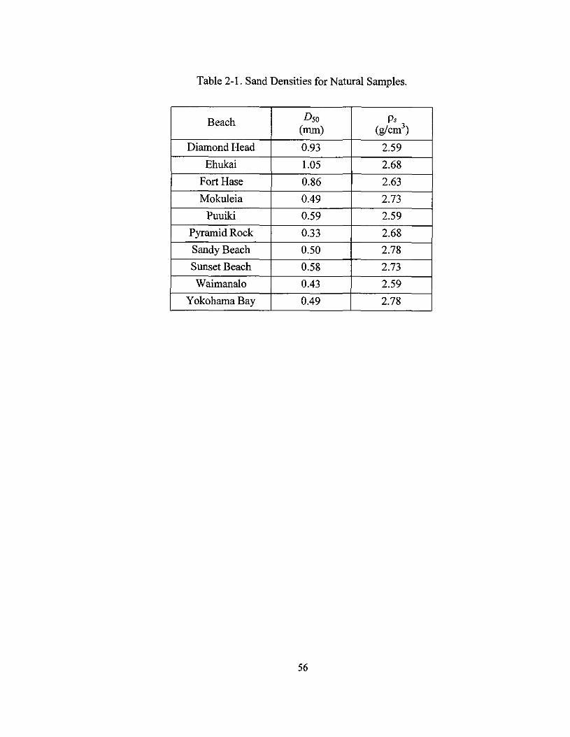
Table 2-1. Sand Densities for Natural Samples.

Beach Dso Ps(nun) (g/cm3

)

Diamond Head 0.93 2.59

Ehukai 1.05 2.68

Fort Hase 0.86 2.63

Mokuleia 0.49 2.73

Puuiki 0.59 2.59

Pyramid Rock 0.33 2.68

Sandy Beach 0.50 2.78

Sunset Beach 0.58 2.73

Waimanalo 0.43 2.59

Yokohama Bay 0.49 2.78

56

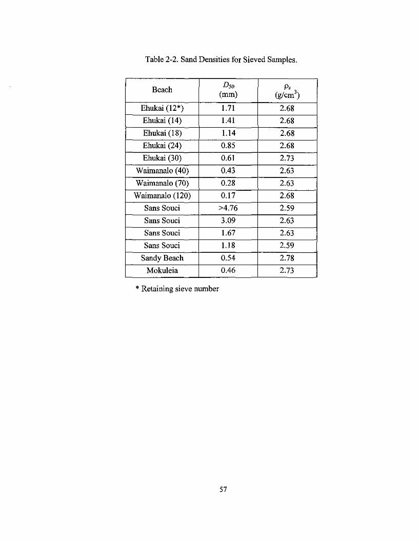
Table 2-2. Sand Densities for Sieved Samples.

BeaehDso Ps

(mm) (g/em3)

Ehukai (12*) 1.71 2.68

Ehukai (14) 1.41 2.68

Ehukai (18) 1.14 2.68

Ehukai (24) 0.85 2.68

Ehukai (30) 0.61 2.73

Waimanalo (40) 0.43 2.63

Waimanalo (70) 0.28 2.63

Waimanalo (120) 0.17 2.68

Sans Souci >4.76 2.59

Sans Souei 3.09 2.63

Sans Souei 1.67 2.63

Sans Souei 1.18 2.59

Sandy Beaeh 0.54 2.78

Mokuleia 0.46 2.73

* Retaining sieve number

57

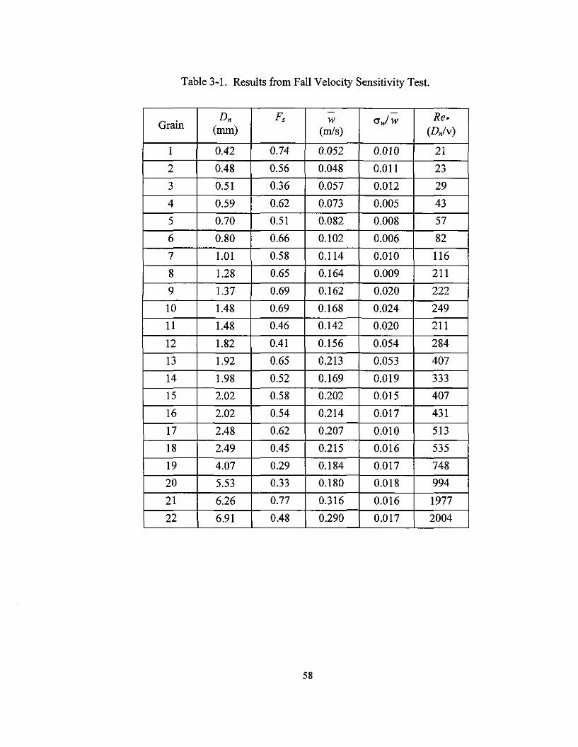
Table 3·1. Results from Fall Velocity Sensitivity Test.

GrainDn Fs w cr,./w Re.

(mm) (m1s) (Dn/v)

1 0.42 0.74 0.052 0.010 21

2 0.48 0.56 0.048 0.011 23

3 0.51 0.36 0.057 0.012 29

4 0.59 0.62 0.073 0.005 43

5 0.70 0.51 0.082 0.008 57

6 0.80 0.66 0.102 0.006 82

7 1.01 0.58 0.114 0.010 116

8 1.28 0.65 0.164 0.009 211

9 1.37 0.69 0.162 0.020 222

10 1.48 0.69 0.168 0.024 249

11 1.48 0.46 0.142 0.020 211

12 1.82 0.41 0.156 0.054 284

13 1.92 0.65 0.213 0.053 407

14 1.98 0.52 0.169 0.019 333

IS 2.02 0.58 0.202 0.Dl5 407

16 2.02 0.54 0.214 0.017 431

17 2.48 0.62 0.207 0.010 513

18 2.49 0.45 0.215 0.016 535

19 4.07 0.29 0.184 0.017 748

20 5.53 0.33 0.180 0.018 994

21 6.26 0.77 0.316 0.016 1977

22 6.91 0.48 0.290 0.017 2004

58

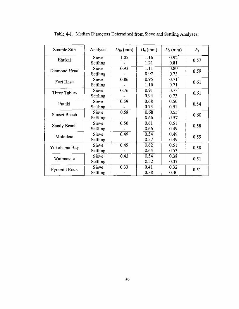
Table 4-1. Median Diameters Detennined from Sieve and Settling Analyses.

Sample Site Analysis Dso (mm) Dn(mm) De (mm) Fs

Ehukai Sieve 1.05 1.16 0.920.57

Settling - 1.21 0.81

Diamond Head Sieve 0.93 1.11 0.800.59

Settling - 0.97 0.73

Fort Hase Sieve 0.86 0.95 0.710.61

Settling - 1.10 0.71

Three Tables Sieve 0.76 0.91 0.730.61

Settling - 0.94 0.73

Puuiki Sieve 0.59 0.68 0.500.54

Settling - 0.73 0.51

Sunset Beach Sieve 0.58 0.68 0.550.60

Settling - 0.66 0.57

Sandy Beach Sieve 0.50 0.61 0.510.58

Settling - 0.66 0.49

Mokuleia Sieve 0.49 0.54 0.490.59

Settling - 0.57 0.49

Yokohama Bay Sieve 0.49 0.62 0.510.58

Settling - 0.64 0.53

Waimanalo Sieve 0.43 0.54 0.380.51

Settling - 0.52 0.37

Pyramid Rock Sieve 0.33 0.41 0.320.51

Settling - 0.38 0.30

59

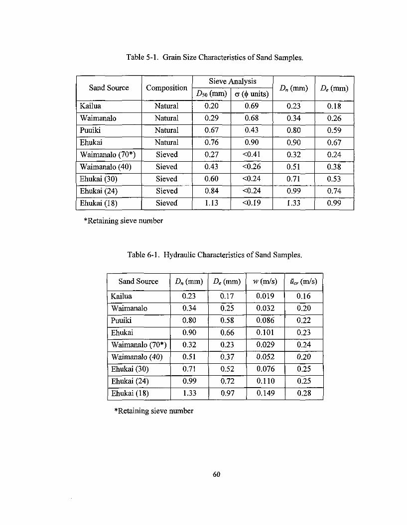
Table 5-1. Grain Size Characteristics of Sand Samples.

Sand Source CompositionSieve Analysis

Dn(mm) De(mm)Dso (mm) cr (~units)

Kailua Natural 0.20 0.69 0.23 0.18

Waimanalo Natural 0.29 0.68 0.34 0.26

Puuiki Natural 0.67 0.43 0.80 0.59

Ehukai Natural 0.76 0.90 0.90 0.67

Waimanalo (70*) Sieved 0.27 <0.41 0.32 0.24

Waimanalo (40) Sieved 0.43 <0.26 0.51 0.38

Ehukai (30) Sieved 0.60 <0.24 0.71 0.53

Ehukai (24) Sieved 0.84 <0.24 0.99 0.74

Ehukai (18) Sieved 1.13 <0.19 1.33 0.99

*Retaining sieve number

Table 6-1. Hydraulic Characteristics of Sand Samples.

Sand Source Dn(mm) De(mm) w(m/s) ucr (m/s)

Kailua 0.23 0.17 0.019 0.16

Waimanalo 0.34 0.25 0.032 0.20

Puuiki 0.80 0.58 0.086 0.22

Ehukai 0.90 0.66 0.101 0.23

Waimanalo (70*) 0.32 0.23 0.029 0.24

Waimanalo (40) 0.51 0.37 0.052 0.20

Ehukai (30) 0.71 0.52 0.076 0.25

Ehukai (24) 0.99 0.72 0.110 0.25

Ehukai (18) 1.33 0.97 0.149 0.28

*Retaining sieve number

60

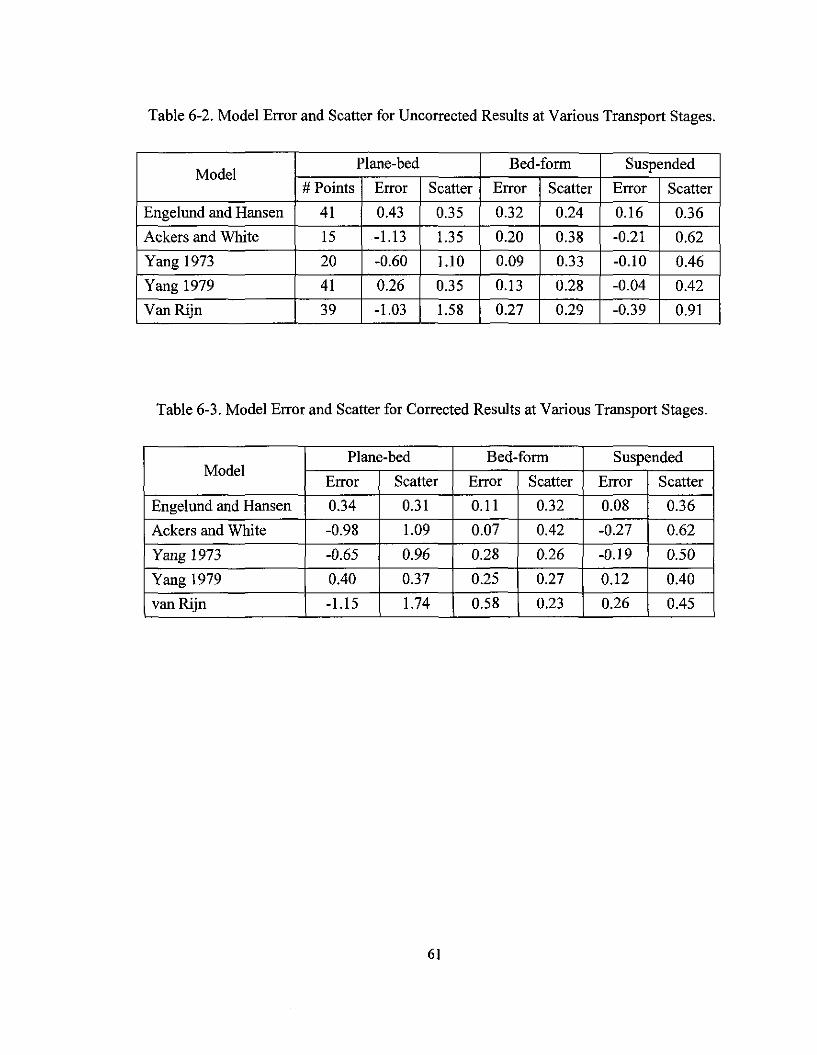
Table 6-2. Model Error and Scatter for Uncorrected Results at Various Transport Stages.

ModelPlane-bed Bed-form Suspended

# Points Error Scatter Error Scatter Error Scatter

Engelund and Hansen 41 0.43 0.35 0.32 0.24 0.16 0.36

Ackers and White 15 -1.13 1.35 0.20 0.38 -0.21 0.62

Yang 1973 20 -0.60 1.10 0.09 0.33 -0.10 0.46

Yang 1979 41 0.26 0.35 0.13 0.28 -0.04 0.42

VanRijn 39 -1.03 1.58 0.27 0.29 -0.39 0.91

Table 6-3. Model Error and Scatter for Corrected Results at Various Transport Stages.

Plane-bed Bed-form SuspendedModel

Error Scatter Error Scatter Error Scatter

Engelund and Hansen 0.34 0.31 0.11 0.32 0.08 0.36

Ackers and White -0.98 1.09 0.07 0.42 -0.27 0.62

Yang 1973 -0.65 0.96 0.28 0.26 -0.19 0.50

Yang 1979 0.40 0.37 0.25 0.27 0.12 0.40

van Rijn -1.15 1.74 0.58 0.23 0.26 0.45

61

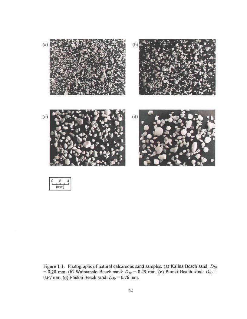
(a)

(c) (d)

Figure 1-1. Photographs of natural calcareous sand samples. (a) Kailua Beach sand: Dso= 0.20 mm. (b) Waimanalo Beach sand: Dso = 0.29 mm. (c) Puuiki Beach sand: Dso =

0.67 mm. (d) Ehukai Beach sand: Dso = 0.76 mm.

62

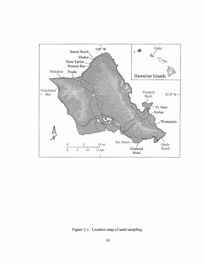
..Oahu

/

Hawaiian Islands

PyramidRock

/

an Souci /

DiamondHead

10 mii I

15 km

5i t i

5 10

oIo

EhukaiThree Tables __Waimea Bay-

Puuiki

1

Figure 2-1. Location map of sand sampling.

63

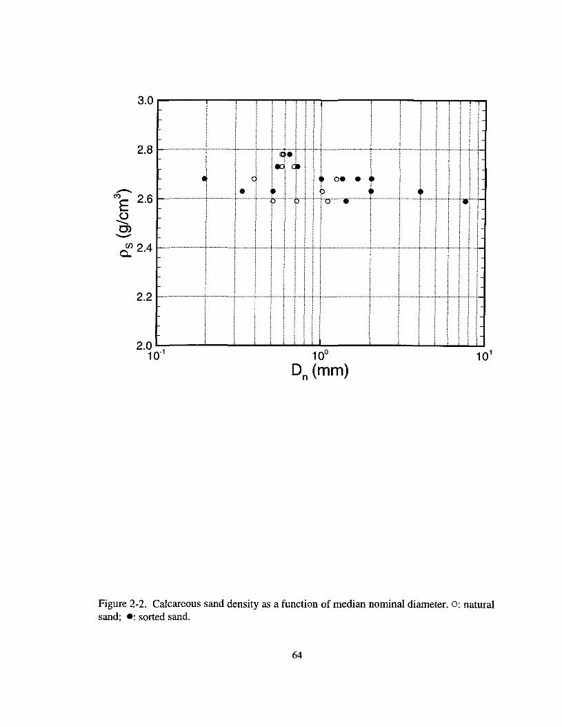
3.0 ....~----r--..,...---r---r--r-T--nr-1T------,----r-----,----,.....,.......,......,...,...,

i ii i

.+....+....+···f ···f····1-

. _-+ + ·+-·····i······1 ···f····1-,

j····1 _+..

,.......+··············1

:··f .._..;._....~._...;_.._j ....l....._._..

,··f············f-·· ····f·······j······f ··-f ··j····f··········,0., , . ,

i i!~~! \\

d" !.o•• ~

, i.:, :' '.L. " .' ",j ,.. •••J..:.. ..l"., ... .1., ...1.,..o : i , :··f ¢ ! 1;,.1' " ••••••••.••••••••+- ·············f ····..··+····..··f ·····t "+.+"'j~

1

"....+..,········f

1

" r,I, I, . .

I ': : ':2.0 '-1__..J...._...J.........J........J......J......L...J.....u_O__....J.._--l..---i----JC-..i.--l....i....LJ 1

10' 10 10

On (mm)

-"'E 2.6 ,-...

-.S?0):r 2.4 - ..........1; ..,

1,,1

j i2.2 _ _+ ··f ··········r + ··+·····!·····f ··;····f····

Figure 2-2. Calcareous sand density as a function of median nominal diameter. 0: naturalsand; .: sorted sand.

64

) ,. ... .

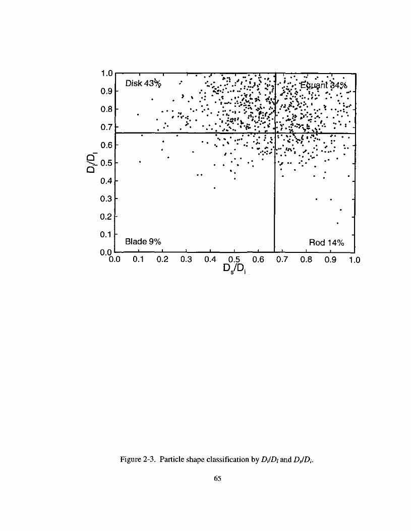
0.9 I-

1.0 r----,----,,----"T'-~'''''-.-7~-""...-.,-T"-_-:••_:.~:y.l.-.·,-:r,-'.:.-":'••'I""-~.-~.:"'1--.--'Disk 43% .' .:..; .' .:'.:''::,;.> ',:. "}:'.: '1::1-'1, ;"'nl ~.'4%_._ •••• ~ .. : ...... )f........

:. :':" ., ••••• I· .... I' .;':-'.:: •• s:.: '.. ', ..-,': .1: .': ,~.. " ('~II .....·t ,'.1" .. " .... " ....... "~:'':'.... " " ~ ,.:.. ... .. : ... . .. ..., ...,.... .. -.' .,-... ..' ~".. ".e............ .. ".e:' ..., ,': ... ···.·.;-.r:t~: .'\>"":~'~' ..... ,• .. .. - , .; ! , .

•'. .. •,-'" •\. ~ ... :.. : .. .. '. e. '. .0.711- -:,..._...::....__-:-:...'_· ·..;.·..;.+-·.:;:'~'.:;::....'~·-,..":":·i"·'_:·~·-_r.~.~.~ ··~,·~·*_:'-f-...~rt· ·-·_:.·;_~-:--1.. • • '.. .. .. " -_- , .. ..", 7· .

• • ' .. 'II ..... : : ~ 1.' ..~ ••~( ••~... '"''.. '. " • • 1- .... "" ••

" . -..... ". ..,',,...: .. .: ~., .. . .e:.:...... -' .. , ... . . . .. .'.. .. : .."....... ....

0.6 I-

0.8 I-

0.5

0.4 I-••

.

0.3

0.2

1.00.9

Blade 9% Rod 14%0.0 L-_.l..-_...l..-_--L._........_---L_.......J'--....L....L..-_...l...-_....J.'------l

0.0 0.1 0.2 0.3 0.4 0.5 0.6 0.7 0.8D/Dj

0.1

Figure 2-3. Particle shape classification by D;lDI and D,ID;.

65

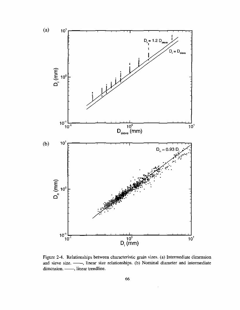
-EE 10°-cf

o =0.930 ..n • ,I .

:' . ....0" :.....

-EE 10°­c:o

10.' L.,----'---'-................................I..JL.,,----'---'-................................l.J10.1 10° 10'

Di (mm)

Figure 2-4. Relationships between characteristic grain sizes. (al Intermediate dimensionand sieve size. --, linear size relationships. (b1 Nominal diameter and intermediatedimension. --, linear trendline.

66

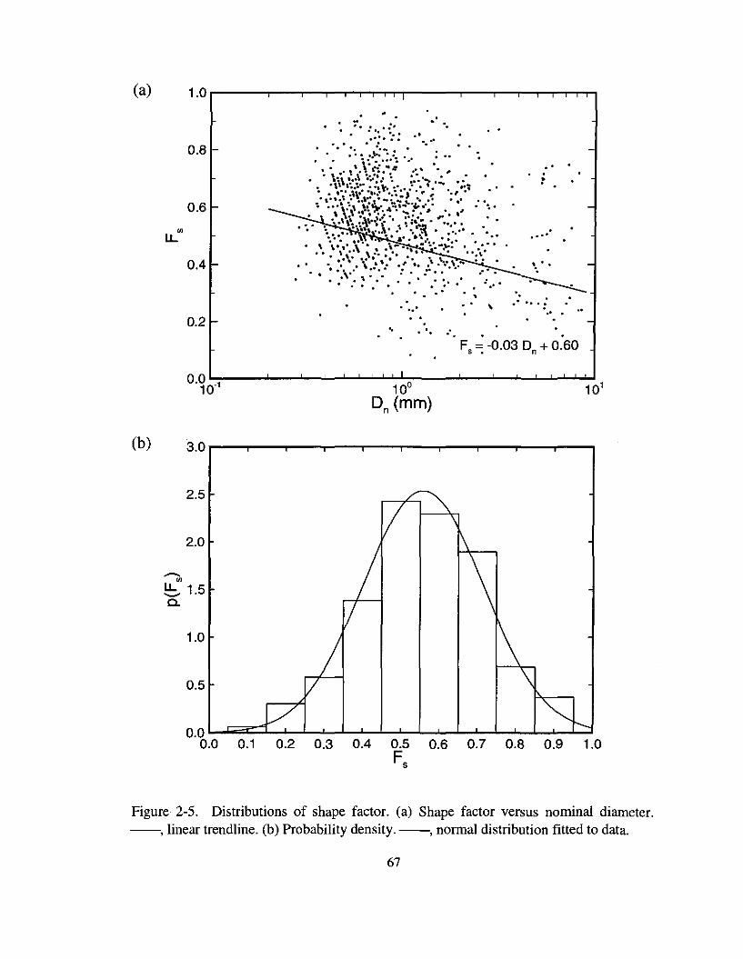
(a) 1.0 .------.---r--r--r-1-r-T'"T"T---r--r--r--T"""""T-r-r..,...,

. .F

S=-0.03 D + 0.60• n

..

.,.

.: -0 • :

.'\

. .

•

. "

. .'

••• 0

.. . .:.".:... ":: .".. .. eo... .

. :: ..;':"*-: ....• ; ':. "0 ••• ~ .0° •

.. "\0·· .'.:, \ ...~.:""{ :::.: :." .:..\\\,...~.. ..• t. 0° ••• 1.... "1••••••\\ )•• ,,#' "0'·., •••~ ••~\ : .. °0 .° "0" "

~ ."',':;, hO,>,,: 40:., .. 0"'.. . • ~.. \ .\.\ ..' ;~ .. ~:: ~ ,,:. ,"... .'.,".,.\ ( .""~. .... ,• \...... "to "~•• ,0 :' '. •••••• "0'

• • I..· "0' •\ \0,· \. .\ ".•••0••••• • ... ,": \ ,,"0 ."0 ."'. • • •• ~ •

• ' • _:".\: ""00

., "I••".'.... \ .... ' •.• '. '0° .0. . :. :".... 00' •

• • 0° : ~ •• ' • •• 0°:"· • 00 •

0.8

0.2

0.4

0.6

'"l.L

0.0 L.,,..-_--'_--'"_.l.-.J..-..................l....L.O,..-_--'_--'"_"'---'-.............L...W 11~ 10 10

Dn (mm)

I/~\

/ \

:1 \

/ \/ \

V ~,

2.0

2.5

0.5

1.0

0.00.0 0.1 0.2 0.3 0.4 0.5 0.6 0.7 0.8 0.9 1.0

Fs

­'"!:S 1.5a.

(b) 3.0

Figure 2-5. Distributions of shape factor. (a) Shape factor versus nominal diameter.--, linear trendline. (b) Probability density. --, normal distribution fitted to data.

67

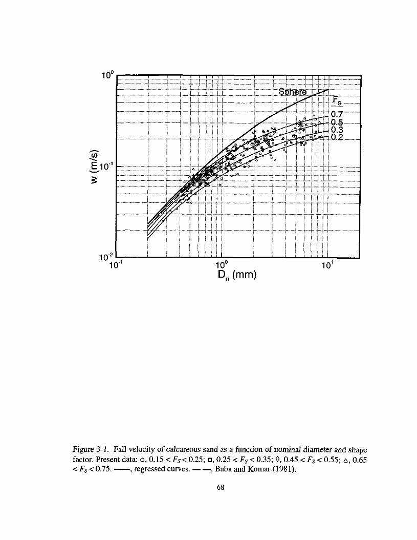
....j ...; ..; ..[ ·r ..... ~...............,

.... j ...; ··i ··f ..... , .... -..........

.: ~ ·····1.-.j .• ·····i ;

! : i·\·······+······i······i·+·j····f···f

, .... :,1 .... , : !........:.. ·······i··· ....····i ..~ ...; .....

1·········

.... j

....• j , ····+····!·····i·····i····j··+··i·····-· ......."-.. ...j. ...j•..•.f.... j ..f... ~...

::.::::::::::!- -----:·1 ::::::L -:::L.:::;::::1::::;:::L.:·························+···········;··········j····+···i·····i····j··++....

........-······i···

························1: : :

.-t ..•:.j j •••

..+ ..+..-} +-.j

: :.......1

"'-Y,' ········f··· ...i-••••• .i-.i

......~ ........, .

,·······1-,

-+ .._._ _.+._ _.~

......-.-.-} -------·-·.,.·········f

··········f··

·············r

-- _.._ ~

100 r-----r--;-...,.......,"T""T'"T"T'T""--..,..---,;-,--T""""T-,-rrT----,··_,··········, .. ·····]"·····"';"····,····[··'1··· ;···············;··········f·······:······:·····,····;._..~._ ...+ -:- - ~ + ··t····:···!· .j....... j'" ; ! .+-+-+ .

··············f :::::..::::~•.::::t.::::t..::!:::!:::J:::l ···················i······· ::::::!::::S~h~:r.~::··r··:::--- :; ~_.. "", ._ ~ ~ ~ ~ j ~ j:...... .. !......: t:f~:::::::::::::

.. i!' ;-~

L--~--1-;t.+:ii fOT------.,'--.,! ..,! --',' 1, :,---','-- ',' -0.-5----------··········T

~:,::2:~.-~E 10-1-

Figure 3-1. Fall velocity of calcareous sand as a function of nominal diameter and shapefactor. Present data: 0,0.15 < Fs< 0_25; c, 0.25 < Fs < 0.35; 0, 0.45 < Fs < 0.55; 6,0.65< Fs < 0.75. --, regressed curves. - -, Baba and Komar (1981).

68

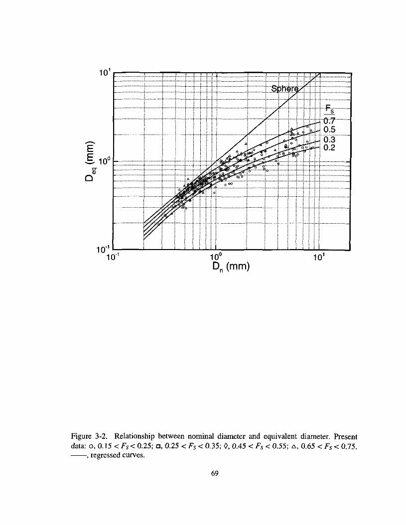
...J .. ~,

····1 ..: 'f'"... j

-'-1 _oj .L-

.....1 i ··i...............1 ············1 .j

... ~ ..~.. ~ ... ~

~i~~;;,~~= .... j ···f .+-+-+_.•• j •••f.+ ++ .

r.. .L.. .. ; , ! ..: ..; .............~..~:_.j .~_ _..!._ ~ . i i000................... . .......•.. • • ····;··.·.·.·,t--_·j "r"';'"

: ; ; , ..: ··f···f···

·1· j .l

••• J. •••t

"-r-'-

..~ - } ). . ~·······t····

········f

.......... .;. ······t ·······T·· ..~

,-'-"'---"1 -+. --- --~ ---+ -+···t .+ +-{

·················f···---

.................. ..J. .;.... ······f··· .. j .......~ ~.•......~ j

..~ ... ·········}··········i·

101 .....--,....-.......,.-,......,,......,.....,....,,...,...,----,-....,...--.,........,.....,...,....,....,.,...--.....,···········.,.·········-r ·,···-;-·····-r····T···T···l··· ,..•.........: , , , j"

:t::::~:!:FEErLr:!:$~h:$r;::ttt. i i : :

···········1· ....•.......;... ······r··---··-:-·····+···..;.···f··+·..;.··· .._ _ _ _._~- , j L.•..;...• l i .: .

..f·lf LL!,. . ;.+ ···!···!I·+++Fs••~ ••~. j j ! ! . . . . .

\;,1'+'\'\':';'0;70.5

.0:3"! 0.2

<TQ)

o

Figure 3-2. Relationship between nominal diameter and equivalent diameter. Presentdata: 0,0.15 < Fs < 0.25; c, 0.25 < Fs < 0.35; 0, 0.45 < Fs < 0.55; <I, 0.65 < Fs < 0.75.--, regressed curves.

69

: !

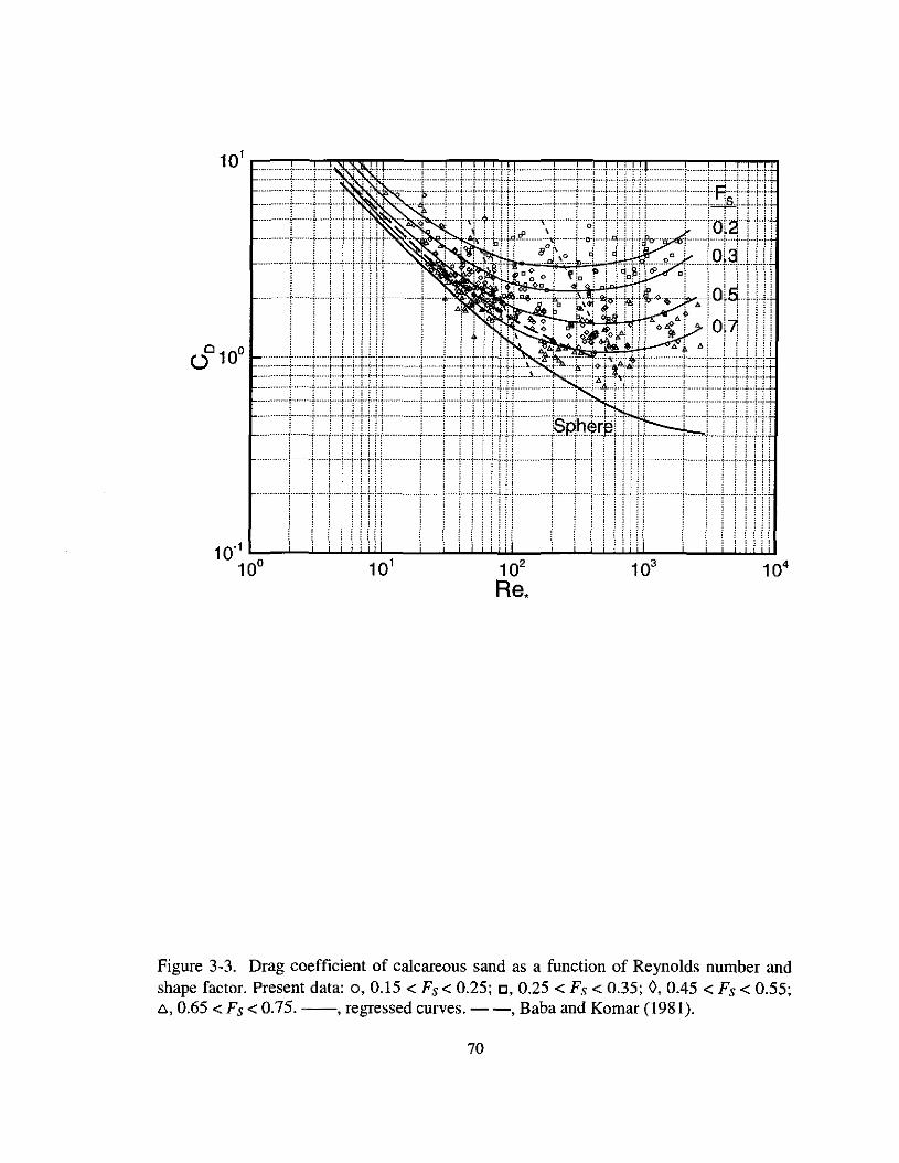
iii iii....l ...L.l..LU l

'0'5':: :i: i ..•..,..,..A: :: ;: i

0 ;,'.'-.:,'.' ; !;;[i ! : ! !

! !] )

, ,, ,

: : :::: : ::.

...... "-....t.; .... ~.'"'-r

t··· "-~"-"r.......;......_~ ..-..~

i ; i;iii i' i: : : ::: :

......~ ..+ + .~ .. ~.;._;-~. _·~_·_··_··i·_· .~.._--+ i-.. ··f····f···;··j··i··i-'· ·············f + +..+++++:

.......•. ·.t l ~-_·~··j··i·-i-j· ;.. ....•.......; ; ;..j .... j - ~ ~ ~..:..j..:..!_.:.._._._.._ +...._..:._.._L.._~ .. ,.__LJ...£.1. •....•. .:.. ..•.........L LLL.L.L:

_...! t ~ ~. .j.. j..).j. '-'T .._,__.! ; .U.ll i _.~ L..:....:...u.·

.......i i ;." iii i ;:;, . ; ;;; ··..··T·· i....•i.. iii:; y.:'i·+H+·ii.'i:n: ······.·.·.·.:.'.:s.·.·.·.n.·.·.-.·.;.h.·.·.·.~.i.·.r.·.·,e.;.·.·.·,'.:.·.·.·..!.·.,.:..,'.; .•·.'.; ,""'"''......+ ....~.....i. ··1 ••U..L.L... ····f· ··f·····~····~···,·· ;,,;·+·i··· . M "P .....;.. "f ··i .~ .u.;. ; ! ! ; !;;; iiiiii i i :: .

.......i oj ----; f ) ..i.j).; .i +····i····i··+ ++H... . +.- j- ··--f i -L-LLU--. l ! J ._) ;.:__j__ ~ :; !;;;; I!! --1 ···········1 !!: I

; iii:iiii ; i

iii i i 1. ..L.j..i.,I.l.:.: .1.: L l l [ 1 :.,__1.. ]. ! i ..1.!..LU.!'r'j"i'i' --r- ·····f "'r

:: ii i.i ! ;.i i.i' i'i

············1 _....•+..-.~............+ ;, .

101r_---;---;...,-.;l""l"'I:"T'TT"-"''T""""''T"""T"T"..,.TT"""-r-~..,.,..,.,.,..r____,____,_""T""",...,.,.,.."

.••••.•.•••• t" •••••• -t- ••••-l'

Figure 3-3. Drag coefficient of calcareous sand as a function of Reynolds number andshape factor. Present data: 0, 0.15 < Fs < 0.25; c, 0.25 < Fs < 0.35; 0, 0.45 < Fs < 0.55;6,0.65 < Fs < 0.75. --, regressed curves. - -, Baba and Komar (1981).

70

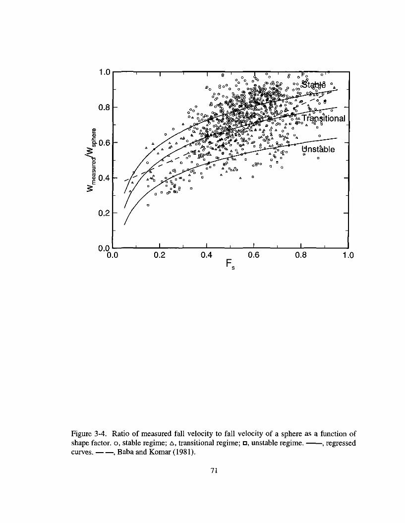
o•

o

". 0

oo

o•"o

oo

• ••• .,po

1.0 '---""'---'--""""'-""'-;;-8...,....-....--0.....,...-::---,;--::-0,.-----,

0.8

0.2

1.00.80.60.40.20.0 L..-_L....----'L....----'_---'_---'_---'_---'_---'_---'_----I

0.0

Figure 3-4. Ratio of measured fall velocity to fall velocity of a sphere as a function ofshape factor. 0, stable regime; 6, transitional regime; c, unstable regime. --, regressedcurves. --, Baba and Komar (1981).

71

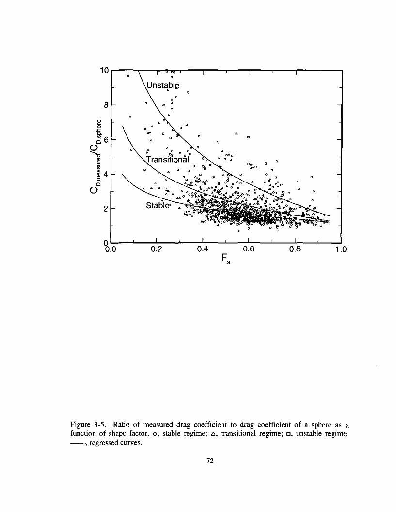
10 00

• 0

0

00

8 00

0

• 0

l'! 0

Ql 0

.<: •a. '" •66

0 0

• •~

• 00 • 0 0 •

.(>. t.G IJ []0'0

l'! Transitional 00

• 0 0

00

::>'\0

0 0

'"0 ",,0

'" 40 • 0

QlE •6 •

0 • • 4>• •

0

2 Statile'

0

00.0 0.2 0.4 0.6 0.8 1.0

Fs

Figure 3-5. Ratio of measured drag coefficient to drag coefficient of a sphere as afunction of shape factor. 0, stable regime; 6, transitional regime; c, unstable regime.--, regressed curves.

72

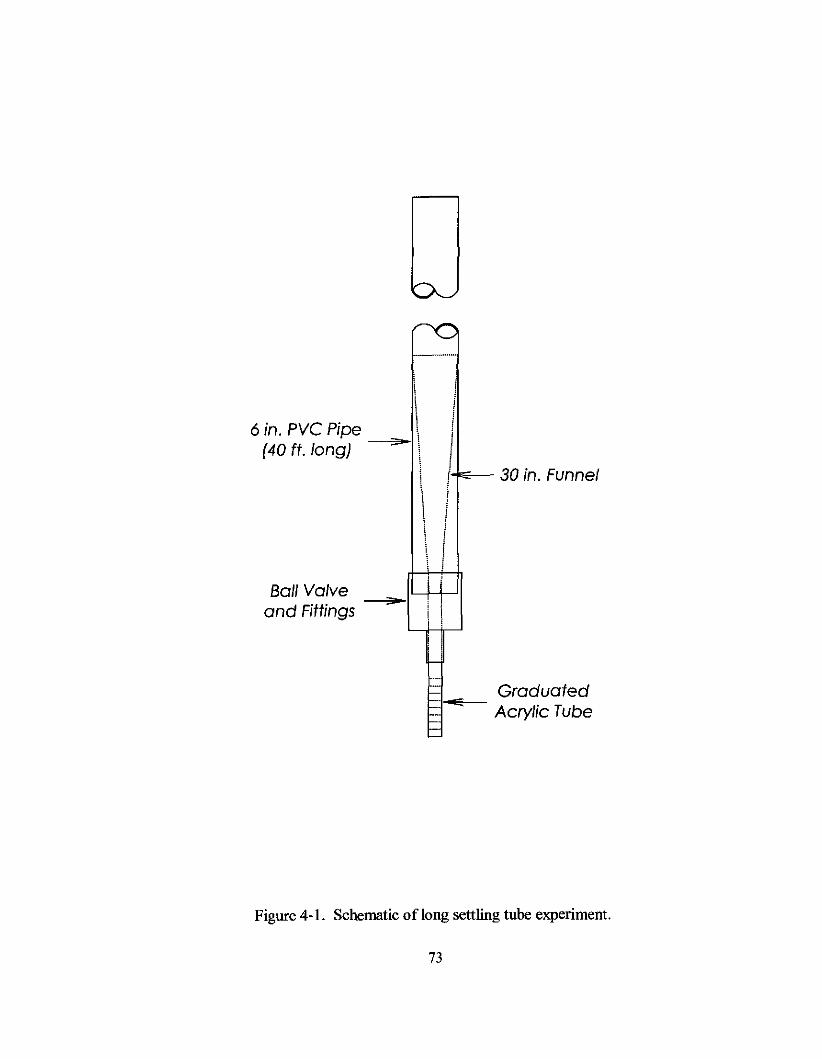
6 in. PVC Pipe \ I(40 ft. long)

;. \ I\ !

I- 30 in. Funnel

\\

{

\1

Ball Valve i iand Fittings

;.I I!

-,

I!i

Graduated:: ne:: Acrylic TUbe

Figure 4-1. Schematic oflong settling tube experiment.

73

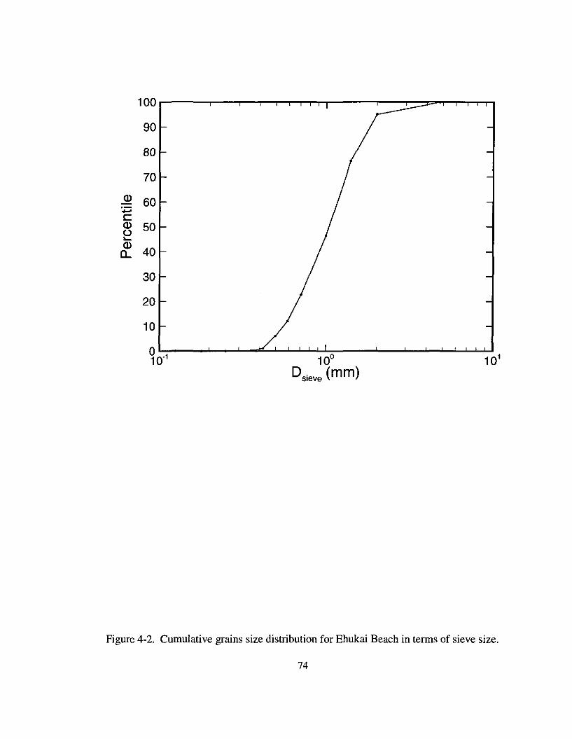
100

90

80

70

Q) 60:;:::::cQ) 50()....Q)

40a..

30

20

10

~0'1 10° 101

DSieve (mm)

Figure 4-2. Cumulative grains size distribution for Ehukai Beach in terms of sieve size.

74

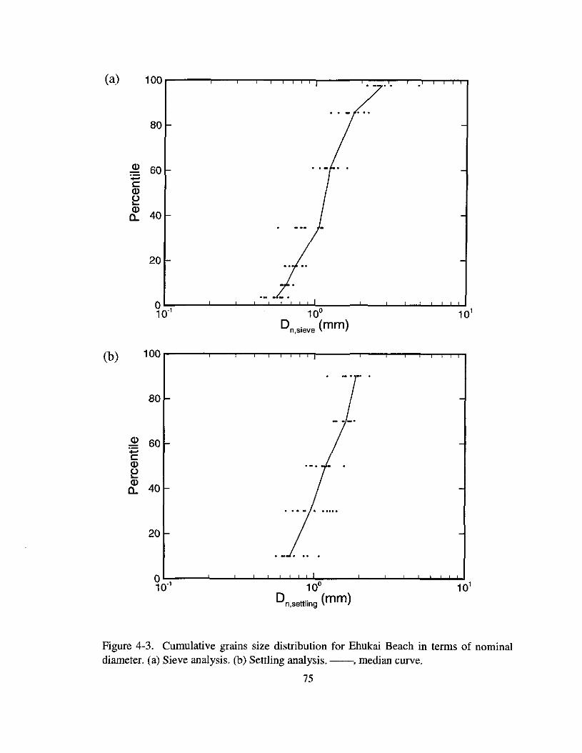
(a) 100 .....----,.---r---,-....,.............,....,............---.-----.----,.......,.....,...-,....,...,....,

80

<1l 60:;:::;C<1l~

rf 40

(b) 100 ...-----,..-..----.--...............,....,....,....,....--..----..---.--.-.,.--,-...,.......,

80

<1l 60..-C<1l~

rf 40

20

100

Dn,settling (mm)10'

Figure 4-3. Cumulative grains size distribution for Ehukai Beach in terms of nominaldiameter. (a) Sieve analysis. (b) Settling analysis. --, median curve.

75

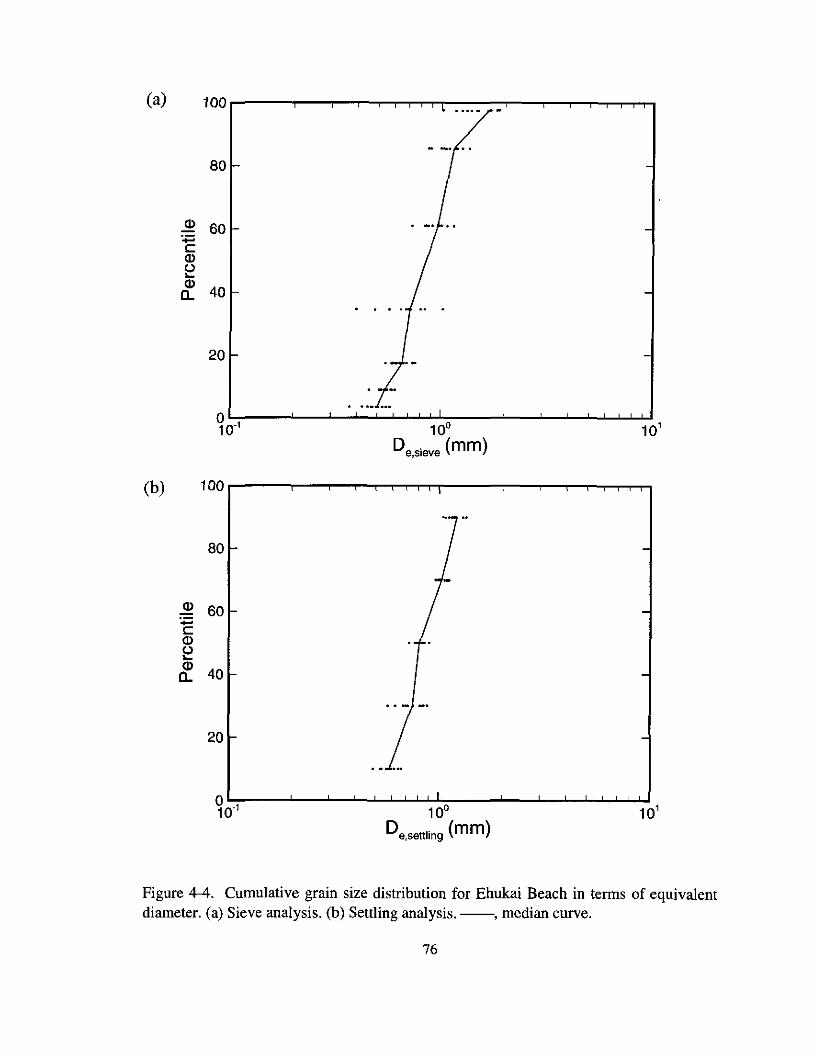
(a) 100 ...----r---r-,....-,.......,.--rT""T'"r-..-..-.-.""'---r-,....-,.......,.....,...."!""'M

80

Q) 60+=cQ)

~

rf. 40

20

10·De,sieve (mm)

10'

(b) 100 ..-----,--.,....-~--,-T"T'"T"T"""--.,....-__.,.____,_....,.....,.......,.....,...,...,

80

Q) 60....cQ)

~Q)

40a... - _.

20

10·De,settling (mm)

10'

Figure 4-4. Cumulative grain size distribution for Ehukai Beach in terms of equivalentdiameter. (a) Sieve analysis. (b) Settling analysis. --, median curve.

76

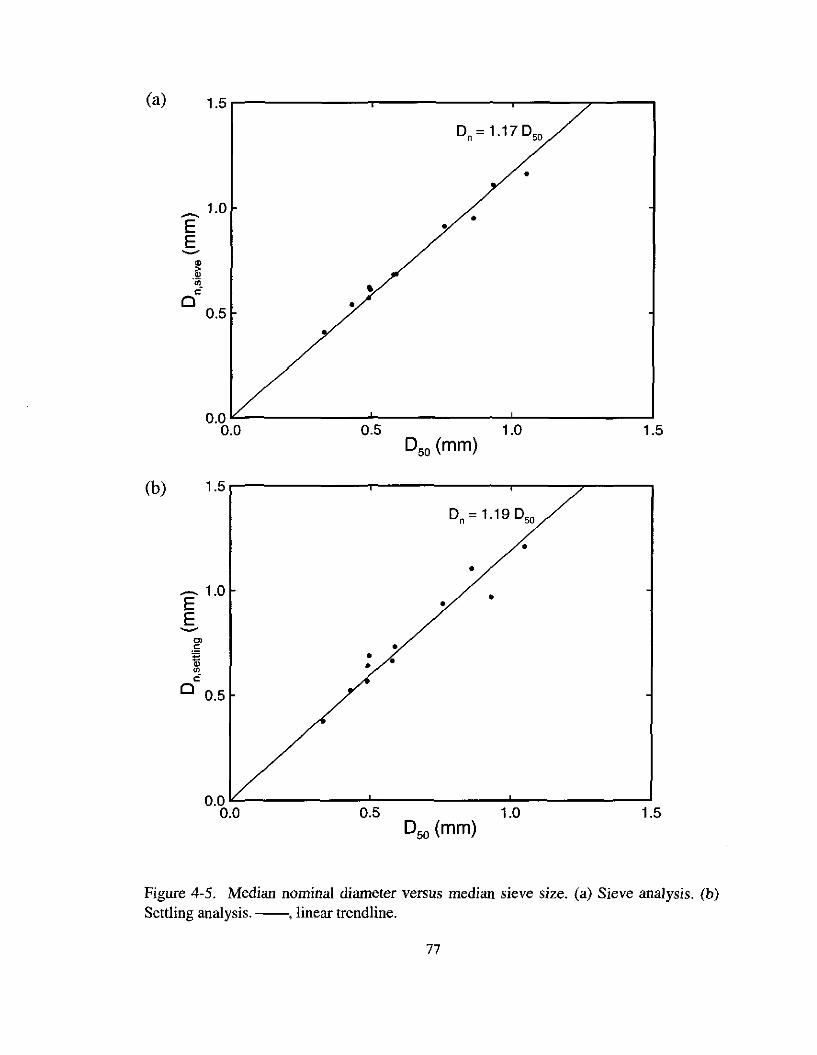
(a) 1.5

°n=1.17050

•

........ 1.0•E •

E---~'iii •,,-

0 •0.5

0.00.0 0.5 1.0 1.5

050 (mm)

(b) 1.5

On = 1.19 050

••

_1.0 •E •E---'".S •i •'" •c:

0 0.5

1.51.00.50.0 ""---------'--------'----------'

0.0050 (mm)

Figure 4-5. Median nominal diameter versus median sieve size. (a) Sieve analysis. (b)Settling analysis. --, linear trendline.

77

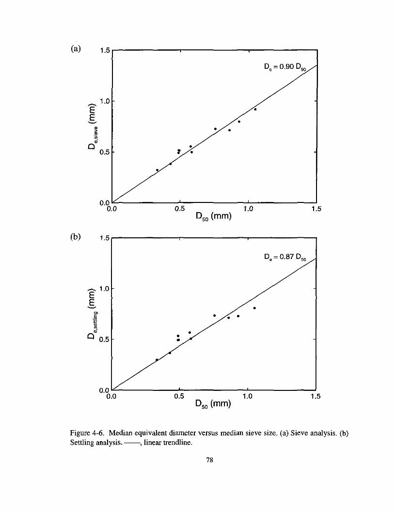
(a) 1.5,....-------,-------,.-------,

De = 0.90 0 50

1.0-E •E •---<II • •iii.'"..-Cl •

0.5 : •

•

1.51.00.5

0.0~ ....... ___J. ___I

0.0D50 (mm)

(b) 1.5r--------r--------,,....-----...,

De =0.87050

_1.0EE--­'".5

~...Cl 0.5 ••

•

• • ••

1.5O.O~-----.......------.......--------'

0.0 0.5 1.0D50 (mm)

Figure 4-6. Median equivalent diameter versus median sieve size. (a) Sieve analysis. (b)Settling analysis. --, linear trendline.

78

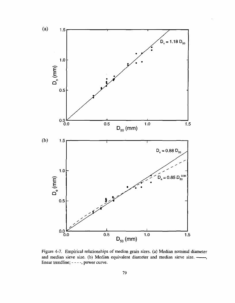
(a) 1.5

Dn = 1.18 D50

•••

1.0 ••-EE •---<= •a ,

0.5

1.51.00.5

0.0 "'-- -'- --1. ----'

0.0050 (mm)

(b) 1.5.....-----.........-----...,--------,

De = 0.88 D50

1.51.0

"" -- -- De = 0.85 D5~·84

.... .,..• •

050 (mm)0.5

1.0

-EE---"a

0.5

"""""/.

0.00.0

Figure 4-7. Empirical relationships of median grain sizes. (a) Median nominal diameterand median sieve size. (b) Median equivalent diameter and median sieve size. --,linear trendIine; - - - -, power curve.

79

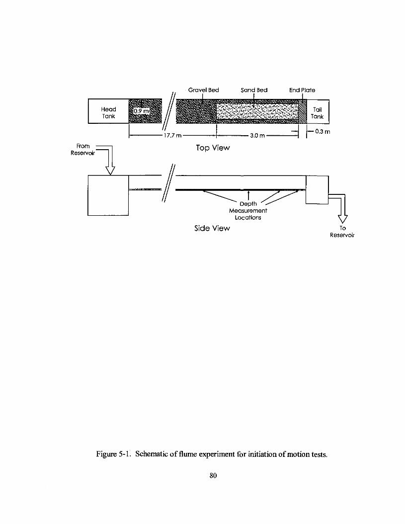
Gravel Bed Sand Bed End Plate

Head TailTank Tank

17.7m 3.0m :1 /-o.3m

From .=­Reservoir

,

Top View

f=.--/~I~Depth L-_-.J

MeasurementLocations

Side View ToReservoir

Figure 5-1. Schematic of flume experiment for initiation ofmotion tests.

80

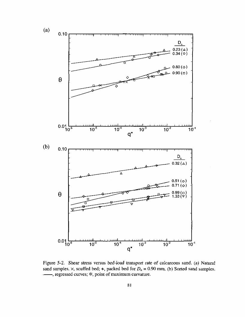
(a)

e<>

0.0'0-6 10-5 10-4 10-3 10.2 10-1

q*

(b) 0.10

~

~

_ 0.32 (t;)A- t;A

e

0.0' 0L..6.,.......,.--'-.J...J.J.J.J1.l.L0

"",_5--'--'-'..>-.J.JUJ

10:-:.7"4-L............u.J.

1UJO-='_3,-'-....L...u.J.l..l.

1u..0

--:;2....L......l...J..l.J.J.1JJJO·'

q*

Figure 5-2. Shear stress versus bed-load transport rate of calcareous sand. (a) Naturalsand samples. x, scuffed bed; +, packed bed for Dn = 0.90 mm. (b) Sorted sand samples.--, regressed curves; *, point of maximum curvature.

81

\ x

x

O.O\OL.,O,....--'--'-................1J.JOi..,1-.J.-.J.-L..l..'-U.1lJ.O..,,2-.L...-~...w...u.J1U.O-:;-3-1...-'--J. ..........L.l.lJ104

Rp

Figure 5-3. Initiation of motion diagram in terms of median equivalent diameter. Presentstudy: ., natural calcareous sand; ., sieved calcareous sand. Paphitis et al. (2002): 0,

mussel particles; +, cockle particles. Prager et ai. (1996): x, calcareous sand. Brownlie(1981): --, Shields curve.

82

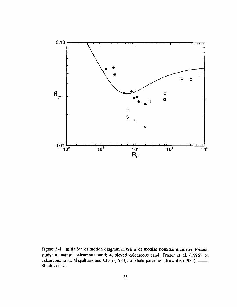
•• D

D

8cr• D

•• D• D•x

~ x

x

0.01 Lo,...-..L-..L-L...l..Ju.J.J.J..,-1............--'-.......u.u...,,2-'--l-L...l....1..u.J..L..,3""--'---.J.......l-J..L...l..l.J.I 410 10 10 10 10

Rp

Figure 5-4. Initiation of motion diagram in terms of median nominal diameter. Presentstudy: ., natural calcareous sand; ., sieved calcareous sand. Prager et al. (1996): x,calcareous sand. Magalhaes and Chau (1983): c, shale particles. Brownlie (1981): --,Shields curve.

83

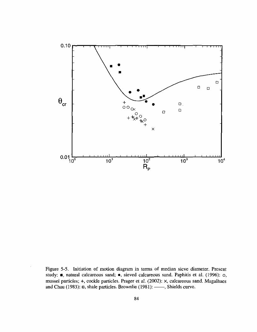
•0

• 0

• ••+ • 0•000<

0

°0

+¥O+<0

+X

0.01 L;o:--.l..-..........u..J...J.J.l,,-l......J.....J...l..U...u.L':;'"2......--L........l..U..J.J.J..3:;--...J...--l.....J-U..J.J.LI 4

10 10 10 10 10Rp

Figure 5-5. Initiation of motion diagram in terms of median sieve diameter. Presentstudy: ., natural calcareous sand; ., sieved calcareous sand. Paphitis et al. (1996): 0,

mussel particles; +, cockle particles. Prager et al. (2002): x, calcareous sand. Magalhaesand Chau (1983): c, shale particles. Brownlie (1981): --, Shields curve.

84

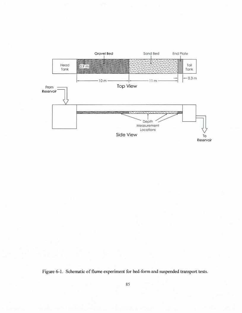
Grovel Bed Sand Bed End Plate

FromReservoir

HeodTonI<

ToilTonI<

-----10 m----------11 m----

Top View

Side View ToReservoir

Figure 6-1. Schematic of flume experiment for bed-form and suspended transport tests.

85

............-,­

.............

.......,.•........

...............-;;.....:.... ..... ..."'...g ...........•... 0 ..P"-~ -

o - ..."o • 0 e ..·:·: 0 " 0 ~..... • .

• 0 D° ,···· 0 .- ~.... .

• .,,~""'. D~er ~ Q ....., ••.•.....

Q......"'.... ....... 0 I~ eP ..'l:JI·····l:JIIo lSI..... • ~ .

..' lID .... .....• .. . .

10' _--'-!"""T"T"I"TT'r'T'"""-r-"""r-T'"T"T"T",--"""'-r-"T'""T""""'nr-...,.--,-r-T""T""t':T-O'I.....................,.

.........., .

......., .

..........-..100

......, .

.................-_.

100

Figure 6-2. Calculated versus measured sediment transport rates using Engelund-Hansen(1967) model. 0, ., plane-bed transport stage; 0, ., bed-form transport stage; t:" a,suspended transport stage (0, 0, t:,: uncorrected; ., ., a, corrected). --, perfectagreement; - - -, factor of 2 difference; ......., factor of 10 difference.

86

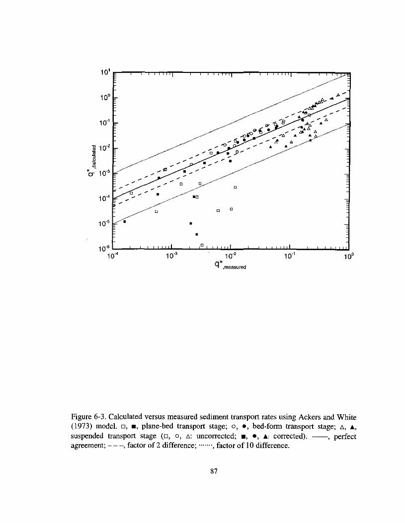
10' .....-r-.,--r-r-.,..,..rTT"-"""T'".....,.....,...,....,..,..,.,..--..--r-,...,....,...,.nT-.....,.---r"""T'".,................•...

....,.•.......

. .

o

oo

. , .~ -_.

.0

o

.,......••..••......

........,.•...•..........

..., .........

...........•...•...•.

..........••...•.........

.......,.•...........

•

•

..........•..,...

.............. ..•..............

········0.•............--

.......•., .

10°

•o10" L..._......J.-J....l.J..L.u.L_.....L.....;,;:..J...J..LJ...UJ-_.l-.......l-l....u..u.I._............L.....L....u..l.u.I

1~ 1~ 1~ 1~'

q*.measured

Figure 6-3, Calculated versus measured sediment transport rates using Ackers and White(1973) modeL 0, ., plane-bed transport stage; 0, ., bed-form transport stage; 1;, .,

suspended transport stage (0, 0, t.: uncorrected; ., ., .: corrected), --, perfectagreement; - - -, factor of 2 difference; , factor of 10 difference,

87

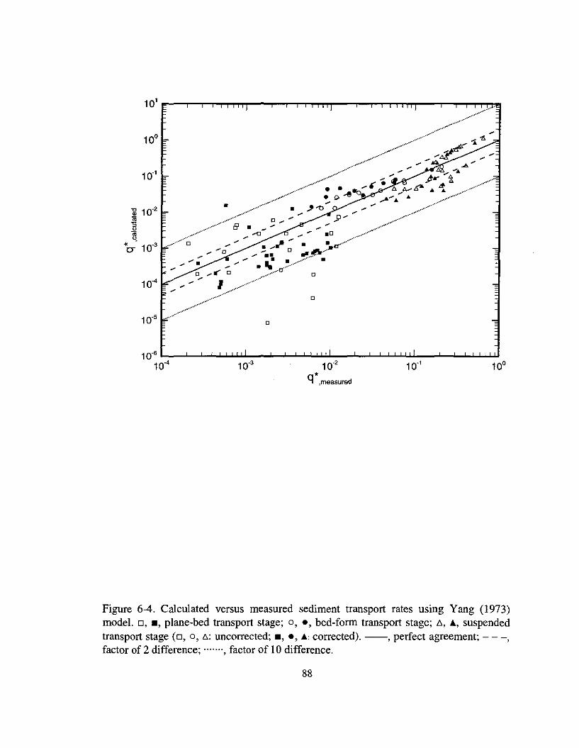
101 ",....-.--,....,,.......,..,..,"T'T"'-......-,.......'T'""T"TTTT"""-.......,.-,....,..TT'T'T'T"--,......,.-,."T'"'!".,..,,.,

..........•., , .

a

a

•

-_........•., .

.......................

.•...•...••, - ..A"'"

/ ~

....._ :... ., ~" .. '" ~~~"'';i .......................... ~ p ..-8 0 .. . .

.... ."'"'0 ... ",.. .••...•....•..••..••.•............••.....OJ • ~ .0 -_.

....",...-'() ......... . ...•.................. • ..... D _of]'

..... a .... -.. ~...e--......... L-· ..,....... .... • .. c:r"'"

" .... 0 ........•••.•••••.

..~ - .

.........................-.....~

...............,....

.......

10°

a

10°

Figure 6-4. Calculated versus measured sediment transport rates using Yang (1973)model. 0, ., plane-bed transport stage; 0, ., bed-form transport stage; t1, A, suspendedtransport stage (0, 0, t1: uncorrected; ., ., A: corrected). --, perfect agreement; - --,factor of 2 difference; ....... , factor of 10 difference.

88

10' ...........,--,r""'T...,...,."TT1,.,....-.......,-.....,..,..,.......-..,-"'T"""T""T...,......TT'T"-...,.....,........,..,.,""""

.........••...•..........

.....•...•............................

..........•, .........

................

.-,-

...........,...,....

........, .

..-..~_ ,............ ....

..............,.....~ ~...i,"O .... :?• • ;... ~ Qoo

• • !2:J ........•...•• D. ~ O..---e.Oo .p9....··· .0 0

·0 ·· .0 6 ........... ...."} 0 .A~ 0 .......

, "··'olP'lSI • D".~ D ......,. 0- I!!!I 0 ~.@ .

.-,.,............

10°

.....•............

10°10.6 L........._L...J.-'-'..u..U-_.l.-.J-~.u.L.l.I-_..J........L-.J....J...u...u.l._...J...........l-l..l..J..J.U

10.4

Figure 6-5. Calculated versus measured sediment transport rates using Yang (1979)model. 0, ., plane-bed transport stage; 0, ., bed-form transport stage; .6, ., suspendedtransport stage (0, 0, .6: uncorrected; ., ., .: corrected). --, perfect agreement; - --,factor of 2 difference; ....... , factor of 10 difference.

89

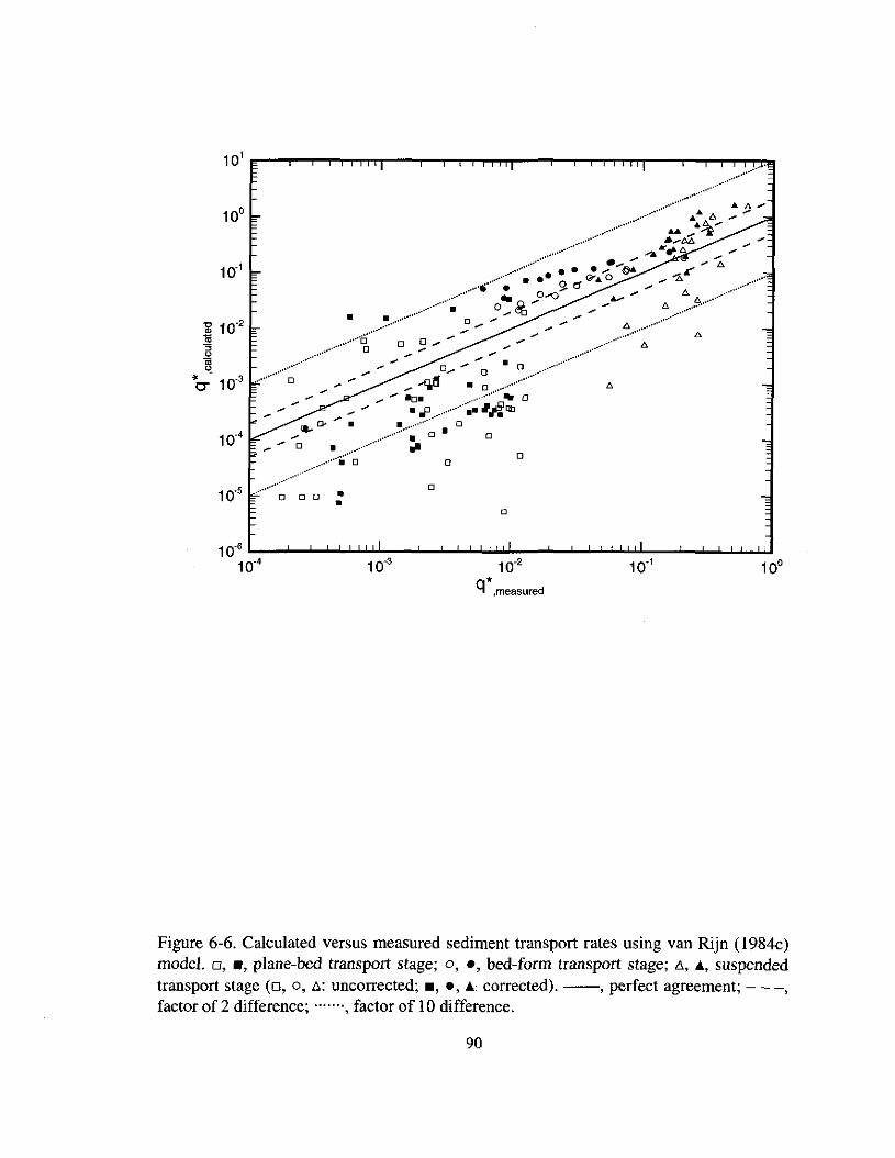
10' 1"'""".....,,...........,....,..,-n"-"""''''''''''''''''T""T''T''T'Tr--r-''''''''''''''''''''rTT"-''''''''''''''''''''''''''''''''''''''.............

o

o

o

o••

.~................................. 6 :. f) ....

....... .t..~.............,.. :;M~

•••••••..••.. - '.ll.~"'lJ. .... ....

........., 0& L' .... l::.............. • .- 0 C1 9".. 0 .... -1..

..,......... 0..-0'" tJ.............;. 0"~ f', ••••••,.~, .. .~ ,......... ~.... - , ,

.- - .... - •••~.•••"...... L'i.............°0.... 0 0....... Do

........ ..., .~ ~ .

o D ..••.....••·

... -0_ ..~.-..~ ;:.,..~• rP .............•- "AQtI

......~ ...~'~ • 0 0

o 00

~

.... <>- •~

...... 0 • ....

............···.···0

.•., ~ .

10°

10°10'6 L-.....---'.................LJ.J.J-_"--.l....J.......l..U.J.l-_...............J...l...u..u.J.._................J.....JU-l..L.U

10'4 10" 10'2 10"

q*,measured

Figure 6-6. Calculated versus measured sediment transport rates using van Rijn (l984c)model. 0, ., plane-bed transport stage; 0, ., bed-form transport stage; /1, ..., suspendedtransport stage (0, 0, t.: uncorrected; ., ., ..., corrected). --, perfect agreement; - --,factor of 2 difference; , factor of 10 difference.

90

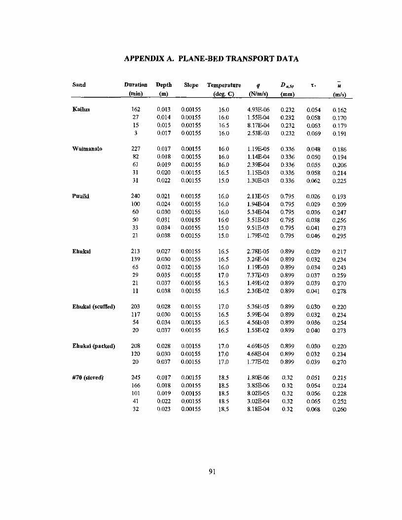
APPENDIX A. PLANE-BED TRANSPORT DATA

Sand Duration Depth Slope Temperature q D R,5Q ,. u(min) (m) (deg. C) (N/mI,) (mm) (mI,)

Kailua 162 0.013 0.00155 16.0 4.93E-06 0.232 0.054 0.16227 0.014 0.00155 16.0 155E-04 0.232 0.058 0.17015 0,0]5 0.00155 16.5 8.l7E-04 0.232 0.063 0.1793 0.017 000155 16.0 2.53E-03 0.232 0.069 0191

Waimanalo 227 0.017 0.00155 16.0 1.19E-05 0.336 0.048 0.18682 0,0]8 0.00155 16.0 1.14E-04 0336 0050 0.19461 0.019 0.00155 16.0 2.39E-04 0.336 0.055 0.20631 0.020 0.00155 16.5 1.15E-03 0.336 0.058 0.21431 0.022 0.00155 15.0 1.30E-03 0.336 0.062 0.225

Puuiki 240 0.021 0.00155 16.0 2.13E-05 0.795 0.026 0.193100 0.024 0.00155 16.0 I.94E-04 0.795 0.029 0.20960 0.030 0.00155 16.0 5.34E-04 0.795 0.036 0.24750 0.031 0.00155 16.0 3.51E-03 0.795 0.038 0.25633 0.034 0.00155 15.0 9.51E-03 0.795 0.041 0.27321 0.038 0.00155 15.0 1.79E-02 0.795 0.046 0.295

Ehukai 213 0.027 0.00155 16.5 2.78E-05 0.899 0.029 0.217139 0.030 0.00155 16.5 3.26E-04 0.899 0.032 0.23465 0.032 0.00155 16.0 1.19E-03 0.899 0.034 0.24329 0.035 0.00155 17.0 7.37E-03 0.899 0.037 0.25921 0.037 0.00155 16.5 1.49E-02 0.899 0.039 0.27011 0.038 0.00155 16.5 2.36E-02 0.899 0.041 0.278

Ehukai (,cutTed) 203 0,028 0.00155 17.0 5.36E-05 0.899 0.030 0.220117 0.030 0.00155 16.5 5. 99E-04 0.899 0.032 0.23454 0.034 0.00155 16.5 4.56E-03 0.899 0.036 0.25420 0.037 0.00155 16.5 1.55E-02 0.899 0040 0.273

Ehukai (packed) 208 0,028 0.00155 17.0 4.69E-05 0.899 0.030 0.220120 0.030 0.00155 17.0 4.68E-04 0.899 0.032 0.23420 0.037 0.00155 17.0 1.77E-02 0.899 0.039 0.270

1170 (,ieved) 245 0.017 0.00155 18.5 1.80E-06 0.32 0051 0.215166 0.018 0.00155 18.5 3.85E-06 0.32 0.054 0.224101 0.019 0.00155 18.5 8.02E-05 0.32 0.056 0.22841 0.022 0.00155 18.5 3.02E-04 0.32 0.065 0.25232 0.023 0.00155 18.5 8.18E-04 0.32 0.068 0.260

91

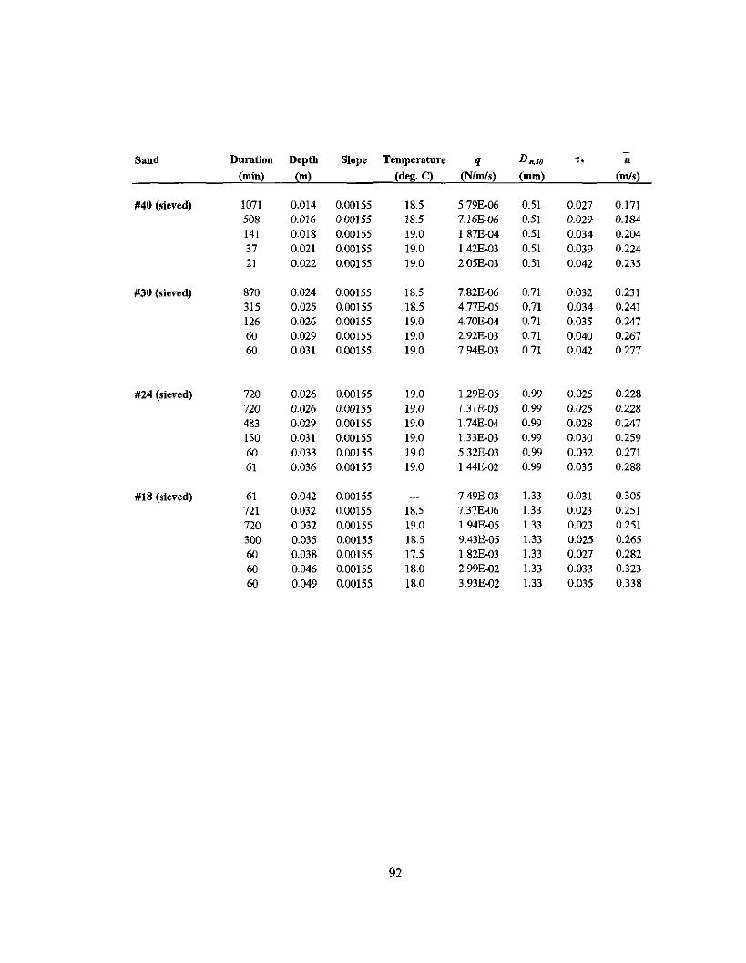
Sand Duration Depth Slope Temperature q D",50 T. U

(min) (m) (deg. C) (Nfml,) (mm) (mI,)

#40 (,ieved) 1071 0.014 0,00155 18.5 5.79E-06 0.51 0.027 0.171508 0.016 0,00155 18.5 7,16E-06 0.51 0.029 0.184141 0.018 0,00155 19,0 1.87E-04 0.51 0.034 0.20437 0.021 0,00155 19,0 1.42E-03 0.51 0.039 0.22421 0.022 0.00155 19.0 2.05E-03 0.51 0.042 0.235

#30 (,ieved) 870 0,024 0.00155 18,5 7.82E-06 0.71 0.032 0,231315 0,025 0.00155 18.5 4.77E-05 0,71 0.034 0,241

126 0,026 0.00155 19.0 4.70E-04 0,71 0.035 024760 0.029 0.00155 19.0 2.92E-03 0,71 0.040 0,26760 0.031 0.00155 19.0 7.94E-03 0.71 0,042 0.277

#24 (,ieved) 720 0.026 0.00155 19.0 1.29E-05 0.99 0.025 0.228

720 0.026 0.00155 19.0 1.31E-05 0.99 0.025 0.228

483 0.029 0.00155 19.0 1.74E-04 0.99 0.028 0.247

150 0.031 0,00155 19.0 1.33E-03 0.99 0.030 0.25960 0.033 0,00155 19.0 5,32E-03 0.99 0.032 0.271

61 0.036 0,00155 19.0 1.44E-02 0.99 0.035 0.288

#18 (,ieved) 61 0,042 0.00155 7.49E-03 1.33 0.031 0305

721 0.032 0.00155 18.5 7.37E-06 1.33 0.023 0,251

720 0.032 0.00155 19.0 1.94E-05 1.33 0,023 0.251300 0.035 0.00155 18.5 9.43E-05 1.33 0.Q25 0.265

60 0.038 0,00155 17.5 1.82E-03 1.33 0.027 0.28260 0046 0.00155 18,0 299E-02 1.33 0.033 0.32360 0,049 0.00155 180 3.93E-02 1.33 0.035 0338

92

APPENDIX B. BED-LOAD AND SUSPENDED-LOAD TRANSPORT DATA

Sand Duration Dn,50 Temperature Depth u q Slope 1'1 )"

(min) (mm) (deg. 9 (m) (mi.) (N/mi.) (m) (m)

Kailua 12 0.232 16.0 0.118 0.304 5.30E-03 7.74E-04 0.0211 0.137010 0.232 16.0 0.137 0.343 1.00E-02 6.87E-04 0.0157 0.127013 0.232 16.5 0.102 0.253 1.42E-03 6.56E-04 0.0206 0.138012 0.232 16.5 0.122 0.295 3.72E-D3 6.15E-04 0.0168 0.140010 0.232 16.5 0.092 0.290 6.57E-03 8.21E-04 0.0135 0.111013 0.232 16.5 0.145 0.326 4.76E-03 6.12E-04 0.0191 0.178011 0.232 16.5 0.111 0.269 2.59E-03 5.57E-D4 0.0150 0.13509.5 0.232 16.5 0.082 0.263 6.68E-03 9.22E-04 0.0185 0.1610

Waimanalo 15 0.336 16.0 0.126 0.403 8.83E-03 473E-04 0.0206 0.186014 0.336 16.0 0.135 0.428 9. 11 E-03 1.23E-D3 0.0218 0.2350

14.5 0.336 16.5 0.145 0.429 1.02E-02 1.13E-03 0.0218 0.21308 0.336 16.5 0.094 0.448 1.44E-02 2.28E-03 0.0203 0.1780

7.5 0.336 16.0 0.097 0.528 2.81E-02 2.40E-03 0.0163 0.351013.5 0.336 16.5 0.122 0.474 1.33E-02 1.52E-03 0.0206 0.445010 0.336 16.5 0.128 0.499 1.50E-02 1.54E-D3 0.0165 0.254011 0.336 16.0 0.111 0.380 7.72E-D3 1.47E-03 0.0274 0.2590

16.75 0.336 17.0 0.Q75 0.281 3.15E-D3 1.27E-03 0.0206 0.1860

Puuiki 10.5 0.795 17.0 0.121 0.527 3.19E-02 2.29E-03 0.0270 0.495022.5 0.795 17.0 0.140 0.455 4.85E-03 8.18E-04 0.0094 0.472047 0.795 17.0 0.088 0.339 2.16E-04 639E-04 0.000078 0.795 18.0 0.120 0.405 1.20E-03 729E-04 0.0074 0.526056 0.795 19.0 0.131 0.429 3.33E-03 1.0TE-03 0.0183 0.498020 0.795 18.0 0.116 0.485 1.14E-02 1.52E-03 0.0155 0.447019 0.795 18.0 0.105 0.462 8.48E-03 1.78E-03 0.0218 0.654027 0.795 18.0 0.081 0.377 1.93E-03 8.84E-04 0.0000

Ehukai 25 0.899 16.0 0.123 0.517 1.40E-D2 1.65E-03 0.0196 0.804024 0.899 16.0 0.115 0.489 7.27E-03 1.49E-03 0.0145 0.582019 0.899 17.0 0.104 0.467 4.58E-03 1.24E-03 0.0102 1.200025 0.899 17.0 0.079 0.377 8.48E-04 1.02E-03 0.000091 0.899 17.0 0.104 0.363 l.39E-04 6.47E-04 0.000048 0.899 18.0 0.140 0.455 3.09E-03 8.18E-04 0.0094 0.697039 0.899 18.0 0.130 0.433 2.19E-03 7.81E-04 0.0086 0.868054 0.899 18.0 0.092 0.403 2.11E-03 9.86E-04 0.0056 1.5000

93

LITERATURE CITED

Ackers, P. (1993). "Sediment transport in open channels: Ackers and White update."Proceeding of the Institution of Civil Engineers, Water, Maritime, & Energy, 10I,247-249.

Ackers, P., and White, W. (1973). "Sediment transport: New approach and analysis."Journal of the Hydraulics Division, ASCE, 99(11), 2041-2060.

Alger, G.R, and Simons, D.B. (1968). "Fall velocity of irregular shaped particles."Journal of the Hydraulics Division, ASCE, 94(3), 721-737.

Baba, J., and Komar, P.D. (1981). "Measurements and analysis of settling velocities ofnatural quartz sand grains." Journal ofSedimentary Petrology, 51(2), 631-640.

Bagnold, RA. (1966). "An approach to the sediment transport problem from generalphysics." U.S. Geological Survey Professional Paper 422-1, Washington, DC, 37 p.

Braithwaite, c.J.R. (1973). "Settling behaviour related to sieve analysis of skeletalsands." Sedimentology, 20(2), 251-262.

Brownlie, W.R. (1981). Prediction of flow depth and sediment discharge in open channels.Rep. No. KH-R-43A, W.M. Keck Lab. of Hydr. and Water Resour., Cal. Inst. Tech.,Pasadena, CA.

Buffington, J.M. (1999). "The legend of A.F. Shields." Journal of HydraulicEngineering, ASCE, 125(4),376-387.

Buffington, J.M., and Montgomery, D.R. (1997). "A systematic analysis of eight decadesof incipient motion studies, with special reference to gravel-bedded rivers." WaterResources Research, 33(8), 1993-2029.

Chang, H.H. (1988). Fluvial processes in river engineering. John Wiley and Sons, NewYork, 456 pages.

Cheng, N.-S. (1997). "Simplified settling velocity formula for sediment particle." JournalofHydraulic Engineering, ASCE, 123(2), 149-152.

Dai, J. (1997). Engineering Characteristics of Tropical Island Beaches. Master's Thesis,Department of Ocean Engineering, University of Hawaii, Honolulu, Hawaii.

De Lange, W.P., Healy, T.R, and Darlan, Y. (1997). "Reproducibility of sieve andsettling tube textural determinations for sand-sized beach sediment." Journal ofCoastal Research, 13(1),73-80.

94

Engelund, F., and Hansen, E. (1967). A monograph on sediment transport. TechniskForlag, Copenhagen, Denmark.

Folk, RL., and Ward, W.C. (1957). "Brazos River bar: A study in the significance ofgrain size parameters." Journal ofSedimentary Petrology, 27(1), 3-26.

Frith, C.A. (1983). "Some aspects of lagoon sedimentation and circulation at One TreeReef, southern Great Barrier Reef." B.M.R Journal of Australian Geology andGeophysics, 8(3),211-221.

Gerritsen, F. (1978). Beach and Surf Parameters in Hawaii. Report No. UNIHI­SEAGRANT-TR-78-02, University of Hawaii Sea Grant College Program, Honolulu,Hawaii.

Giigu~, M., ipek~i, O.N., and Kiikpinar, MA (2001). "Effect of particle shape on fallvelocity of angular particles." Journal of Hydraulic Engineering, ASCE, 127(10),860-869.

Hardisty, J. (1990). Beaches: Form and Process. Unwin Hyman, London, 324 p.

Hamey, J.N., Grossman, E.E., Richmond, B.M., and Fletcher III, C.H. (2000). "Age andcomposition of carbonate shoreface sediments, Kailua Bay, Oahu, Hawaii." CoralReefs, 19(2), 141-154.

Janke, N.C. (1966). "Effect of shape upon the settling velocity of regular convexgeometric particles." Journal ofSedimentary Petrology, 36(2), 370-376.

Jell, J.S., Maxwell, W.H.G., and McKellar, RG. (1965). 'The significance of the largerforaminifera in the Heron Island reef sediments." Journal of Paleontology, 39(2),273-279.

Kench, P.S., and McLean, RF. (1996). "Hydraulic characteristics of bioclastic deposits:new possibilities for environmental interpretation using settling velocity fractions."Sedimentology, 43(3), 561-570.

Kench, P.S., and McLean, R.F. (1997). "A comparison of settling and sieve techniquesfor the analysis of bioclastic sediments." Sedimentary Geology, 109(1-2), 111-119.

Komar, P.D., and Cui, B. (1984). "The analysis of grain-size measurements by sievingand settling tube techniques." Journal ofSedimentary Petrology, 54(2),603-614.

Komar, P.D., and Reimers, C.E. (1978). "Grain shape effects on settling rates. Journal ofGeology, 86(2), 193-209.

Kramer, H. (1935). "Sand mixtures and sand movement in fluvial models." Transactions,American Society ofCivil Engineers, 100,798-878.

95

Lavelle, J.W., and Mofjeld, H.O. (1987). "Do critical stresses for incipient motion anderosion really exist?" Journal ofHydraulic Engineering, ASCE, 113(3), 370-385.

Lipp, D.G. (1995). Changes in Beach Profiles due to Wave Reflections off Seawalls atLanikai, Hawaii. Master's Thesis, Department of Ocean Engineering, University ofHawaii, Honolulu, Hawaii.

Lund-Hansen, L.C., and Oehmig, R. (1992). "Comparing sieve and sedimentationbalance analysis of beach, lake, and eolian sediments using log-hyperbolicparameters." Marine Geology, 107(1-2), 139-147.

Magalhaes, L., and Chau, T.S. (1983). "Initiation of motion conditions for shalesediments." Canadian Journal of Civil Engineering, 10(3),549-554.

Maiklem, W.R. (1968). "Some hydraulic properties of bioclastic carbonate grains."Sedimentology, 10(2), 101-109.

Mantz, P.A. (1977). "Incipient transport of fine grains and flakes by fluids-extendedShields diagram," Journal of the Hydraulics Division, ASCE, 103(6),601-615.

McNown, J.S., and Malaika, J. (1950). "Effects of particle shape on settling velocity atlow Reynolds numbers." Transactions. American Geophysics Union, 31(1), 74-82.

Mehta, A.J., Lee, J., and Christensen, B.A. (1980). "Fall velocity of shells as coastalsediment." Journal ofthe Hydraulics Division, ASCE, 106(11), 1727-1744.

Milan, DJ., Heritage, G.L., Large, A.R.G., and Brunsdon, C.F. (1999). "Influence ofparticle shape and sorting upon sample size estimates for a coarse-grained uplandstream." Sedimentary Geology, 129(1-2),85-100.

Miller, M.C., McCave, LN., and Komar, P.D. (1977). "Threshold of sediment motionunder unidirectional currents." Sedimentology, 24(4), 507-527.

Miller, P.R. (1998). Evaluating Existing Cross-shore Sediment Transport Models for aSteep, Porous Beach, Waimea Bay Beach, Oahu, Hawaii. Master's Thesis,Department of Ocean Engineering, University of Hawaii, Honolulu, Hawaii.

Moberly, R. (1963). Coastal Geology of Hawaii. Report No. 41, Hawaii Institute ofGeophysics, University of Hawaii, Honolulu, Hawaii.

Moberly, R., and Chamberlain, T. (1964). Hawaiian Beach Systems. Report No. 64-2,Hawaii Institute of Geophysics, University of Hawaii, Honolulu, Hawaii.

Paintal, A.S. (1971). "Concept of critical shear stress in loose boundary open channels."Journal ofHydraulic Research, 9(1), 91-113.

96

Papanicolaou, A.N., Diplas, P., Evaggelopoulos, N., and Fotopoulos, S. (2002)."Stochastic incipient motion criterion for spheres under various bed packingconditions." Journal ofHydraulic Engineering., ASCE, 128(4),369-380.

Paphitis, D., Collins, M.B., Nash, L.A., and Wallbridge, S. (2002). "Settling velocitiesand entrainment thresholds of biogenic sands (shell fragments) under unidirectionalflow." Sedimentology, 49(1), 211-225.

Prager, EJ, Southard, J.B., and Vivoni-Gallart, E.R. (1996). "Experiments on theentrainment threshold of well-sorted and poorly sorted carbonate sands."Sedimentology, 43(1), 33-40.

Sagga, A.M.S. (1992). "The use of textural parameters of sand in studying thecharacteristics of coastal sediments south of Jeddah, Saudi Arabia." Marine Geology,104(1-4),179-186.

Sanford, RB., and Swift, D.J.P. (1971). "Comparison of sieving and settling techniquesfor size analysis, using a Benthos Rapid Sediment Analyser." Sedimentology, 17(3-4),257-265.

Scoffin, T.P. (1987). An Introduction to Carbonate Sediments and Rocks. Blackwell,Glasgow, 274 p.

Sengupta,S., and Veenstra, H. (1968). "On sieving and settling techniques for sandanalysis." Sedimentology, 11(1-2), 83-98.

Shields, A.F. (1936). Application of similarity principles and turbulence research to bed­load movement. Hydrodynamics Laboratory Pub. No. 167, W.P. Ott and J.C. vanVchelen, trans., V.S. Dept. of Agriculture, Soil Conservation Service, CooperativeLaboratory, Cal. lnst. Tech., Pasadena, CA.

Shore Protection Manual. 1984. Vol. I & II, U.S. Army Corps of Engineers, WaterwaysExperiment Station, Vicksburg, Mississippi.

Shultz, E.F., Wilde, RH., and Albertson, M.L. (1954). "Influence of shape factor on fallvelocity of sedimentary particles." Report prepared for V.S. Army Corps of Engineers,Missouri River Division, through Colorado A&M Research Foundation, Fort Collins,Colorado.

Sneed, E.D., and Folk, RL. (1958). "Pebbles in the lower Colorado River, Texas; a studyin particle morphogenesis." Journal ofGeology, 66(2), 114-150.

Song, C.C.S., and Yang, C.T. (1982). "Minimum energy and energy dissipation rate."Journal ofthe Hydraulics Division, ASCE, 108(5), 690-706.

Swamee, P.K., and Ojha, C.S.P (1991). "Drag coefficient and fall velocity ofnonspherical particles." Journal ofHydraulic Engineering, ASCE, 117(5), 660-667.

97

Task Committee on Preparation of Sedimentation Manual. (1966). "Sedimenttransportation mechanics: initiation of motion." Journal of the Hydraulics Division,ASCE, 92(2), 291-314.

van Rijn, L.C. (1984a). "Sediment transport, Part I: Bed load transport." Journal ofHydraulic Engineering, ASCE, 110(10), 1431-1456.

van Rijn, L.C. (1984b). "Sediment transport, Part II: Suspended load transport." JournalofHydraulic Engineering, ASCE, 110(11), 1613-1641.

van Rijn, L.c. (1984c). "Sediment transport, Part III: Bed forms and alluvial roughness."Journal ofHydraulic Engineering, ASCE, 110(12), 1733-1754.

van Rijn, L.C. (1993). Principles of sediment transport in rivers, estuaries and coastalseas. Aqua Publications, The Hague, The Netherlands, 13 chapters.

Verrecchia, E.P., Freylet, P., Julien, J., and Baltzer, F. (1997). "The unusualhydrodynamic behaviour of freshwater oncolites." Sedimentary Geology, 113(3-4),225-243.

Wadell, H. (1932). "Volume, shape, and roundness of rock particles." Journal ofGeology, 40(5), 443-451.

WadeIl, H. (1933). "Sphericity and roundness of rock particles." Journal of Geology,41(3),310-331.

Waterways Experiment Station. (1935). Studies of river bed materials and theirmovement with special reference to the Lower Mississippi River. Paper i7, ArmyCorps of Engineers, Vicksburg, MS.

Wentworth, C.K. (1922). "A scale of grade and class terms for clastic sediments."Journal ofGeology, 30(5), 377-392.

White, SJ. (1970). "Plane bed thresholds of fine grained sediments." Nature, 228, 152­153.

Yang, C.T. (1973). "Incipient motion and sediment transport." Journal of HydraulicEngineering, ASCE, 99(10), 1679-1704.

Yang, C.T. (1979). "Unit stream power equations for total load." Journal of Hydrology,40(1-2), 123-138.

Yang, C.T. (1996). Sediment transport: Theory and practice. McGraw-Hill, New York,396 p.

Yang, C.T., and Huang, C. (2001). "Applicability of sediment transport formulas."international Journal ofSediment Research, 16(3),335-353.

98

Zapka, M. (1984). Sand Island Sediment Accumulation Study. Master's Thesis,Department of Ocean Engineering, University of Hawaii, Honolulu, Hawaii.

Zingg, T. (1935). "Beitrag zur Schotteranalyse; Die Schotteranalyse und ihre Anwendungauf die Glattalschotter." Schweizerische Mineralogische und PetrographischeMitteilungen, 15(1),39-140.

99