- -- - -------~-

UNIVERSITY OF HAWAII LIBRARY

DATA DRIVEN APPROACH FOR FAULT DETECTION AND IDENTIFICATION USING COMPETITNE LEARNING

A THESIS SUBMITTED TO THE GRADUATE DNISION OF THE UNNERSITY OF HAW AI'I IN PARTIAL FULFILLMENT

OF THE REQUIREMENTS FOR THE DEGREE OF

MASTER IN SCIENCE

IN

ELECTRICAL ENGINEERING

MAY 2006

By Ashish Babbar

Thesis Committee:

Vassilis L.Syrmos, Chairperson ToddR. Reed

Thaddeus P. Dobry

"

•

We certify that we have read this thesis and that, in our opinion, it is satisfactory in scope

and quality as a thesis for the degree of Master of Science in Electrical Engineering.

, • ,

c \\~~1\~1~~~:\\\\\\\\11\~~1\\~\1\\\\\1~\\\ 'I 10 002605488 .

IJN'NERSITY OF H"'W~II ___________

HAWN f , Q111 ,

.H3 \ , no. 4048

, I

fHESIS COMMITTEE

2f-=-I-F"-:f ! b ~ > ~ • I

Chairperson

. ~~ /<?/(-J2 , .

, ~~ •

11

,

ACKNOWLEDGEMENTS

I would first like to thank my advisor Dr. Vassilis L. Syrmos, for his knowledge, support,

guidance, and encouragement throughout my M.S. program at the University of Hawai'i. \

I am also grateful to my committee members: Dr. Todd R. Reed and Dr. Tep Dobry, for

their help and valuable suggestions towards this thesis.

This work is dedicated to my parents who have been the source of inspiration and

encouragement in my life. They have been the foundation of who I am today and every

success I achieve is a tribute to them. On a personal note, I would like to thank my sisters

Namrata and Shelly who have taught me that hard work and perseverance helps to

achieve every goal in life.

And lastly, I would also like to thank my office mates Estefan Ortiz, Xudong Wang,

,Michael West and Hui Ou for their help and support; it was a pleasure working with

them.

\11

• ,. TABLE OF CONTENTS •

ACKNOWLEDGEMENTS

LIST OF FIGURES

LIST OF TABLES

ABSTRACT

1 INTRODUCTION

2 COMPETITIVE LEARNING TECHNIQUES

2.1 Unsupervised Competitive Learning ........................................ .

2.2 Drawbacks of using Unsupervised Competitive Learning ............... .

2.3 Avoiding dead units ........................................................... .

2.4. Conscience Learning Technique ............................................. .

2.5 Frequency Sen..sitive Competitive Learning ................................. .

2.6 Self Organizing Maps ......................................................... .

2.6.1 Competitive Stage ................................................... .

2.6.2 Cooperative Stage ................................................... .

2.7 Primary advantages of using Competitive learning ....................... .

3 CLUSTERING

3.1 Types of clustering ............................................................ .

3.2 K-means clustering ........................................................... .

3.3 Decision on number of clusters .............................................. .

4 FAULT DETECTION AND IDENTIFICATION SCHEME

4.1 Two level approach for clustering .......................................... .

IV

iii

vi

viii

ix

1

7

7

9

10

11

13

14

16

17

19

20

21

24

25

27 , 27

4.2 Why use two level approach for clustering................................. 28

4.3 Reference distance analysis................................................ ... 29

5 SIMULATION RESULTS 33

5.1 VTOL Aircraft ModeL......................... ................................ 33

5.2 Analysis using Unsupervised Competitive learning............ ............ 36

5.3 Analysis using Frequency Sensitive Competitive learning.......... ..... 42

5.4 Analysis using Conscience Learning Technique.... ....................... 46

5.5 Analysis using Self organizing maps........................................ 51

5.6 Performance comparison of different algorithms.......................... 55

6 CONCLUSIONS 58

6.1 Summary........................................................................ 58

6.2 Future work..................................................................... 59

REFERENCES 60

v

LIST OF FIGURES

1.1 Gradient based lea;ning.................... ......................................... ... 3

1.2 Competitive learning........... ........................................................ 5

2.1 Block Diagram of unsupervised learning.................... ........................ 7

2.2 SOM neural network model.......................................................... 16

3.1 Dendrogram of a set of 13 points in I-D space................. ............... ..... 22

3.2 Plot of error vs. number of clusters............ ................................... ... 26

4.1 Two level approach.. ............................................... ............... .... 27

4.2 Example of reference distance calculation using Gaussian data example. ..... 30

4.3 Block Diagram for the Fault Detection and Identification scheme...... ........ 32

5.1 Failure scenario for VTOL Aircraft model......................................... 36

5.2 Clustering of nominal data in training phase using UCL.......................... 37

5.3 Plot of the training data and cluster centers using UCL....................... .... 38

5.4 Clustering of unknown data in test phase using UCL............................. 39

5.5 Trained neurons and cluster centers for the test phase using UeL........... ... 39

5.6 Plot of test data and cluster centers using the UCL ..... .............. ... ...... ... 40

5.7 Detection of data clusters in fault using UCL ..................................... 41

5.8 Test data and 'clusters detected in fault using UCL................................ 41

5.9 Clustering of nominal data in training phase using FSCL........... .............. 42

5.10 Plot ofthe training data and cluster centers using FSCL. .................. , ...... 43

5.11 Clustering of unknown data in test phase using FSCL....................... ..... 44

5.12 Plot of the test data and cluster centers using FSCL........... .............. ....... 44

5.13 .Detection ofthe data clusters in fault using FSCL.................................. 45

5.14 Plot of test data along with clusters detected in fault using FSCL..... ...... .... 46

5.15 Clustering of nominal data in training phase using CL T ................... ,. .... 47

5.16 Plot of the training data and cluster centers using CLT........................... 47

5.17 Clustering of unknown It est data in test phase using CLT.. ...................... 48

5.18 Test data set and corresponding cluster centers using CLT............... .... ... 49

5.19 Identification of the faulty data clusters from the test data set using CLT..... 49

vi

5.20 Plot of test data and clusters detected in fault using CLT................... ..... 50

5.21 Clustering of nominal data in training phase using SOM................... ..... 51

5.22 Plot of the training data and cluster centers using SOM... ........ ....... ......... 52

5.23 Clustering of un know nit est data in test phase using SOM. .................. ..... 52

5.24 Plot ofthe test data and cluster centers using SOM..... ... ......... ..... ............ 53

5.25 Detection of the data clusters in fault using SOM.......................... ........ 54

5.26 Plot of test data along with clusters detected in fault using SOM....... ..... ... 54

5.27 Plot of data set used for test phase showing data points associated with different modes...... ...... ......... ............................................ ........ 55

VlI

LIST OF TABLES

3.1 Within and between cluster distances............................................... 21

5.1 System matrices for nominal and fault modes ...................... :.............. 36

viii

.- _.... .~

•

ABSTRACT

Condition Based Maintenanc~ (CBM) is the process of executing repairs or taking

corrective action when the objective evidence indicates the need for such actions or in

other words when anomalies or faults are detected in a control system. The objective of

Fault Detection and Identification (FDI) is to detect, isolate and identify these faults so

that the system performance can be improved.

When condition based maintenance needs to be performed based on just the data

available from a control system then Data Driven approach is utilized. The thesis is

focused on the data driven approach for fault detection and would use: (i) Unsupervised

Competitive Lea~ing, (ii) Frequency Sensitive Competitive Learning, (iii) Conscience

Learning and (iv) Self Organizing Maps for FDI purpose. , •

This approach would provide an effective Data reduction technique for FDI so that

instead of using the complete data set available from a control sys!em, pre-processing of

the available data would be done using vector quantization and clustering approach. The

effectiveness of the developed algorithms is tested using the data available from a

Vertical Take off and Landing (VTOL) aircraft model.

•

IX

CHAPTERl

INTRODUCTION

A typical control syste~ consists of four basic elements: the dynamic plant,

controllers, actuators and sensors, which work in closed loop configuration. Any kind of

malfunction in these components can result in unacceptable anomaly in' overall system

performance. They are referred to as faults in a control system and according to their

physical locations, they can be classified as dynamic faults, controller faults, actuator

faults and sensor faults. The objective of Fault Detection and Identification (FDl) is to

detect, isolate and identify these faults so that the system performance can be recovered.

Condition based maintenance (CBM) is the process of executing repairs when the

objective'evidence indicates the need for such actions [I]. Model based CBM approaches

can be applied when we have a mathematical model of the system to be monitored. When

CBM needs to be performed based on just the data available from the sensors, data driven

methodologies are utilized • for the purpose. Data-driven approaches are based on

statistical and learning techniques from the theory of pattern recognition [2]. These range

from multivariate statistical methods, competitive learning methods based on neural

networks, equiprobable mapping, self-organizing maps (SOM), signal analysis, and fuzzy

rule-based systems. The advantage of data-driven techniques is their ability to reduce the

computational complexity for the FD I scheme. The main drawback of data-driven

approaches is that their effectiveness is highly dependent on the quantity and quality of

the sensor data.

The idea used in this thesis is that knowing the data available from a particular

• control system, a learning process would be used to train a set of neurons which would

represent the entire data set. Thus in effect instead 'Of using the entire data set for training

and analysis purposes only the trained neurons would be used. This would provide a great

advantage in terms of computational load reduction and provide faster analysis and a

more robust FDI scheme. For training the neurons to provide an adequate representation

of the available data various learning schemes are available. Two important learning

processes: 1) Gradient Based Learning and 2) Competitive Learning are discussed in

detail.

The Competitive learning approach is followed in this thesis and algorithms such

\. as Unsupervised Competitive Learning (UCL) and its improvements Conscience

Learning technique (CL T), Frequency Sensitive Competitive Learning [3] along with

Kahonen's Self Organizing Maps [4] are discussed. In this thesis the effectiveness of the

Competitive learning methods as a data driven approach for FDI would be demonstrated

using the data obtained by the failure of sensors and actuators introduced in a Vertical

Take Off and Landing (VTOL) aircraft model [5],[6].

1.1 Gradient Based Learning:

The goal of this learning process is to adjust the positions of the output neurons so

that the distances between them, in input space coordinates, are proportional to the

distances between the corresponding input neurons, also in input space coordinates. The

architecture is shown in Figure 1.1. This network structure is also known as the

• Willshaw-von der Malsburg model [3] .

2

Output layer

Input layer

Figure 1.1 Gradient Based Learning

Let A and B be two dimensional lattices, termed the input and output lattices,

respectively. To each neuron j corresponds a two-dimensional position in the input space

v, IV) = (w,i' IV,, ). There are two pathways by which activ ity is conveyed. In the first

pathway, activ ity spreads laterally in the input lattice from the active input neuron i to

• other, previously inactive input neuron j :

( 1.1.1)

With 11 .11 the Euclidean Distance and fa monotonically decreasing function, lo r example a

Gaussian . In the second pathway, the initially active input neuron i signals to its output

3

neuron i' that it should initiate a similar spread of activity in the output lattice (the prime

, symbol is used to indicate'the output neurons). As a result of activity spreading in the

output layer, the activity of unit}' becomes:

Act)' = /(m II WJ' -W,' II) ( 1.1.2)

With m a (constant) factor relating the activity spread functions of the input and output

lay:rs ("magnification factor"). The difference between the activity levels in two layers:

(1.1.3)

is then used as an error signal to move positions wJ' of the output units f. The positions

are incrementally updated as follows:

ilw)'J =17{w,'J-w/J)errorj,

(1.1.4)

With 17 the learning rate, a small positive constant, and with ilwJ'J representing the value

with which the, current position wj'Jwill be incremented (including the sign),

1.2 Competitive Learning:

The basic idea underlying "Competitive" learning is as follows: Assume a

sequence of input samples vet) E V, with V ~ 9{d the d-dimensional input space and t the

time co-ordinate and a lattice A of N neurons, labeled i = 1,2, ........ ,N and with the

corresponding weight vectors w,(t)=[ W,(t)]EV, If v(t) can be simultaneously

4

compared with each weight vector of the lattice then the best matching weight, for

example w. , can be determined and updated to match or even better the current input: ,

W,(t + I) ~ W,(t) + L\w, (I), ( 1.2 .1)

The network architecture for the competitive learning is as shown in Figure 1.2.

The network structure is often referred to as the Kohonen 's model since the Self

Organized Map algorithm for topographic map formation is applied to it. The common

input all neurons receive is d irectly represented in the input space, v E V . The winning

neuron is labeled as ( . Its weight vector is the one that best matches the current input

(vector) .

V '-..J

Input layer v

Figure 1.2 Competitive Learning

5

The comparison is commonly based on the dot product,

(1.2.2)

with T the transpose, or on the Euclidean distance between the input vector and the

weight vectors of the lattice, Ilw;-vll. Hence, after the best matching weight vector is

updated, iv. (t+ l)v(t) > w. (t)v(t), or II w. (t+l)-v(t) 11<11 w. (t)-v(t) II respectively. As a I I t I

result of the competitive learning, different weights will become tuned to different

regions in the input space.

This remaining part of this thesis is organized as follows: In Chapter 2 all

competitive learning algorithms i.e. VCL, CL T, FSCL and SOM are introduced. A

complete description of these algorithms along with advantages of using them IS

discussed. The Clustering approach using k-means algorithm and two level approach for

clustering is discussed in Chapter 3. The complete FOI scheme used in the thesis based

on competitive learning is described in Chapter 4. In Chapter 5 the description of the

VTOL model and performance evaluation of the proposed FOI sche~e as applied to the

data obtained from this model is done. Finally, it summary of results and some ideas for

future work are presented in Chapter 6.

. .

. <

6

CHAPTER 2

COMPETITIVE LEARNING TECHNIQUES

Basic neural network algorithms like the Unsupervised Competitive Learning

(UCL), and its modifications like' Conscience Learning Technique (CLT), Frequency

Sensitive Competitive Learning (FSCL) and Self Organizing Maps (SOM) [3],[4] show

great promise in fault detection and identification when the data from the control system

is available as the input i.e. data driven approach. In this chapter a detail explanation of

these algorithms is provided. In addition the advantages of using these approaches for

FDI are discussed.

2.1 Unsupervised Competitive Learning

In unsupervised learning there is no external teacher or critic to oversee the

learning process, as indicated in the Figure 2.1 [7]. Rather, provision is made for a task

independent measure of the quality of representation that the network is required to learn,

and the free parameters of the network are optimized with respect to that measure. Once

the network has become trained to the statistical regularities of the input data, it develops

the. ability to form internal representation for encoding feature of input and thereby to

create new classes automatically.

Environment

Vector describing state, ,-______ --, of the environment

Learning System

Figure 2.1 Block Diagram of unsupervised learning

7

To perform unsupervised learning we use the competitive learning rule discussed

in Chapter I. We use a neural network consisting of two layers- an input layer and a

competitive layer. The input layer receives the available data set. The competitive layer

consists of neurons that compete with each other (in accordance with a learning rille) for

the "opportunity" to respond to features contained in the input data. In its simplest form •

i.e. UCL; the network operated on a "winner takes all" strategy [3].

The main idea behind UCL is to select M neurons (map units) which would be

used to represent the N data samples. The input data samples are thus represented by M

neurons and provide a reduction in computational load for the following procedure. Let

v = (v" v" .... , vd ) <;;; lRd be the input patterns and the neurons are represented by prototype

vectorsw, =[W'pW'2' ..... ,w;J]; i=I,2, ..... ,M and d is the input vector dimension. A

random input sample is first drawn and the Euclidean distance between this sample and

all neurons is calculated. The neuron which is closest to the selected input sample is

termed as the winning neuron.

(=min{llv-w, II} , (2.1.1 )

The weight of the winning neuron is updated using:

w. =W. +7J(v-w.) " , (2.1.2)

The same procedure is repeated for the entire training length and the input data samples

are represented by the M neurons. The trained neurons would then be clustered at level 2

using K-means algorithm, which is discussed in detail in Chapter 3.

8

2.2 Drawbacks of using VeL:

For Unsupervised Competitive Learning the weight density at c0l1vergence is not

a linear function of the input density p(v) and hence the neurons of the map will not be

active with equal probabilities (i.e. the map is not equiprobabilistic). For a discrete lattice

of neurons, it is expected that for N --> co and for minimum MSE quantization, in d-

dimensional space, the weight density will be proportional to:

J

I...'. pew,) oc p d (v) (2.2.1)

In summary UeL tends to under sample the high probability regions and over sample the

low probability ones. In other words it is unable to provide a "faithful" representation of

the probability distribution that underlies the input data.

This limitation leads to the generation of topographic maps where the weight

density pew,) is proportional to the input density p(v) , or where the lattice neurons

should have an equal probability. to be active. In other words the map should be

equiprobabilistic. From an information theoretic point of view such map transfers the

maximum amount of information available about the input distribution. Equiprobabilistic

maps are desired in the following applications:

1. Modeling sensory coding

2. Non parametric Blind source Separation

3. Density estimation e.g. clustering or classification purposes.

4. Feature extraction.

9

2.3 Avoiding Dead Units

The desire to build equiprobabilistic maps was originally not motivated by

information theoretic considerations. As pointed out by Grossberg [8] and Rumelhart and

Zipser [9], one problem with VCL is that it can yield neurons that are never active ("dead .'

units"). These units will not sufficiently contribute to the minimization of the overall

Mean Square Error (MSE) distortion of the map and hence, this will result in a less

"optimal" usage of the maps resources.

Rumelhart and Zipser proposed two methods to solve this problem. The first was

originally introduced by Grossberg and it suggested the addition of an adaptive threshold

to each unit: when a unit wins the competition~ its threshold is increased so that it

becomes less likely to win the competition in the near future; when a unit loses the

competition its threshold is lowered. In other words each unit has a "conscience" and the

goal is to achieve an equiprobabilistic map. By adding the "conscience" one can escape

from the local minima. Examples of this approach are Conscience Learning Technique

(CLT) and Frequency Sensitive Competitive Learning (FSCL) [3].

In their second method Rumelhart and Zipser suggested not only to update the

"winning" unit but also the "losing". units, although with a smaller learning rate. Then a

unit that has always been losing gradually moves towards the mean of the sample

distribution until, eventually it succeeds in winning the competition occasionally as well.

This scheme is called "leaky learning." However its drawback is that for each input

sample, all weights need to be updated. Another way to avoid dead units is to arrange the

un!ts in a geometrical manner, for example, in a lattice with a rectangular topology, and

update the weights of the neighboring losers as well. In other words, one can use a

10

neighborhood function. Example.of such approach is Self organizing Maps (SOM) [4].

When the neighborhood range is decreased too rapidly during the SOM learning phase,

dead units can still occur but the performance is still much better than using the UCL

approach.

2.4 Conscience Learning Technique

The idea behind conscience learning is as follows: When a neural network is

trained with unsupervised competitive learning on a set of input vectors that are clustered

into N groups/clusters then a given input vector v will activate neuron i' that has been

sensitized to the cluster containing the input vector, thus providing a I-out-of- N coding

of that input. However if some region in the input space is sampled more frequently than

the others, then a single unit begins to win all competitions for this region. This leaves the •

remaining N -1 neurons to partition the less frequently accessed regions thus yielding a

less optimal encoding scheme. To counter this defect, one records for each neuron i the

frequency:with which it has won competition in the past c, , and adds this quantity to the

Euclidean distance between the weight vector w, and the current input v , and one defines

the "winner" as follows:

II wi" -v II +c,. s II Wi -v II +c" '<ii, (2.4.1)

As a result of this, units that have won the competition too often will have the tendency to

reduce their winning rates and vice versa.

In Conscience Learning, as it is introduced by DeSieno [10], two stages are

distinguished. First, the winning unit is determined out of the N units:

II

i' = argmin'oL"N II w, -v II' (i.e. a minimum Euclidean distance rule), In the case of a tie

the unit with the lower index wins the competition. Second, and contrary to the UCL, the

winning unit ( is not necessarily the one that will have its weight vectors updated since

the determination of which neuro!1s need to be updated depends on an additional term for

each unit, which is related to the number of times the unit has won the competition in

recent past. Let IF, be the frequency term for the ith unit. It is computed in the following

manner:

IFn~ = IFold + B (, _IFnld) "f i

I I ':1r i ' , (2.4.2)

With ~, the code membership function: ~,= I ,wheni '" i' , else~, = 0, and B a constant,

0< B« I . The latter should be chosen in such a manner that the IF,s stabilize despite of

the fluctuations caused by the randomly chosen input samples v; DeSieno recommends

here B=O.OOOI [10]. Furthermore a bias term c is defined for each unit: , ,

(2.4.3)

with C the bias factor. When taking into account the winning frequency of each unit, a

winning unit t in the Conscience learning format is defined as the one for which:

Ilw. _vii' +c, $llw _vii' +c,,"fi, , , (2.4.4)

The weights are then updated in the same way as In the standard VCL rule

Equation 2.1.2. In summary, a "conscience" is achieved by relating the definition of the

winning neuron to its probability of being the winner (i.e. activation probability). Note

that DeSieno's learning scheme relies on the choice of three parameters. In his examples,

he takes 1] =0.01 to 0.5, C=IO and B=O.OOOI. However stabilizing the learning

12

algorithm can be tricky: it sometimes results in all the "conscience" being taken by a

small number of units only [II].

A slightly modified, yet much simpler version was introduced by Van den Bout

and Miller [12]. The rule of update is as follows for each neuron the number of times it

has won the competition is recorded, and. a scaled version of ~his quantity, a bias in fact,

is added to the distance metric used in the (modified) minimum Euclidean distance rule:

II w,. -v II +Cc,. ~ II w, -y II +Cc, 'di, (2.4.5)

With c, the number of times neuron i has won the competition, and C the scaling factor

(the "conscience factor''). After determining the winning neuron t its "conscience" is

incremented: c. <-- c .. + I. The weight of the winning neuron is updated using: , ,

L'lw" =I](v-w,.) (2.4.6)

Where 'I] is the learning rate and its value is equal to a small positive constant. The

values for C and I] can be varied to get a good stabilization of the equiprobable map.

Thus by using Conscience learning we have avoided the occurrence of dead units i.e.

neurons which are never active and thus the equiprobable map generated are efficient.

2.5 Frequency Sensitive'Competitive Learning

Another conscience based learning scheme that depends on the distortion based •

learning is the Frequency Sensitive Competitive Learning [13]. The learning scheme

keeps a record of the total number of times each neuron has won the competition during

training, Ci. The distance metric in the Euclidean distance rule is then scaled as follows: •

Ilw,.-vllxc,.~llw,-Yllxc" 'di EA. (2.5.1 )

13 •

<.

After the selection of the winning neuron, its conscience is incremented and the weight

vector updated using the standard unsupervised competitive learning rule:

(2.5.2)

Contrary towhat was originally assumed, FSCL does not achieve an equipr<;bable

2

quantization. FSCL basically yields p(w,) oc p(V)3, in the one dimensional case and in

the limit of an infinite number of neurons, a result which is considered favorable since it

is closer to equiprobabilism than what is achieved by standard unsupervised competitive

learning.

2.6 Self Organizing Maps ,

SOM is an unsupervised neural network technique that finds wide application in

pattern recognition, data correlation and visualization of data sets. SOM offers a platform

for data driven methodologies towards fault detection. It is an excellent tool in

exploratory data mining. It projects the input space on prototypes of low-dimensional

regular grid that can be effectively utilized to visualize and explore properties of data.

This ordered grid can be used as a convenient visualization surface for showing different

features of the SOM (and thus of the data).

When the number of SOM units is large, to facilitate quantitative analysis of the

map and the data, similar units need to be grouped, i.e., clustered. Clustering of SOM was

studied and involved in this thesis for two reasons:

1. Reduction of computational load.

2. Drawing inferences from a group of data. ~

14

•

,

Clustering is basically carried out as a two level approach, where the data set is

first clustered using the SOM, and then the SOM is clustered. The most important benefit

of this procedure is that the computational load decreases considerably, making it

possible to cluster the large data sets and to consider several different preprocessing

strategies in a limited time.

SOM is thus used to process the data and extract the prototype vectors which

represent the data set. These prototype vectors preserve the topology of the input data.

We investigate the ability of SOM to detect system faults by comparison of distance

between the prototype vectors of the unknown data and training (nominal) data. Due to

intrinsic properties of the prototype vectors only a few vectors need to be analyzed for

anomalies.

Thus SOM is another improvement over the standard VCL rule as in this case

instead of updating just the "winning" neuron the neighboring neurons would also be

updated an~ hence provided a reduction in the Mean square error and provide better

quantizatio~. In the purest form, the SOM algorithm distinguishes two stages: the

competitive stage and the cooperative stage. In the first case, the best matching neuron is

selected, that is, the "winner", and in the second stage the weights of the winner are

adapted as well as those of its immediate lattice neighbors (cooperation). Hence, in

Kahonen's approach, the neighborhood relations are moved from the activation to the

weight update stage.

15

2.6.1 Competitive Stage

The SOM consists of a regular, two dimensional grid of map units as shown in

Figure 2.2. All neurons receive the same input vector v E V with V ~ md the input

space. Each unit i is represented by a prototype vector Wi (t! = [Wd (I), .... , Wid (t) 1 ; where d

is input vector dimension.

Output Layer (2-D Grid)

Input layer

W,(t) w,(t) w3(t)

Figure 2.2 SOM Neural Network Model

Given a data set the number of map units is firsi chosen. The Map units (neurons)

can be selected to be approximately equal to --iN to S--iN, where N is the number of data

samples in the given data set. The number of Map units determines the accuracy and

generalization capability of the SOM. Increase in the number of map units can provide

better results but an optimum value is decided depending on the number of data samples

which thus reduces the computational complexity. During training the SOM forms an

elastic net that folds onto the cloud formed by the input data. Data points lying near each

other in the input space are mapped onto nearby map units.

16

, i

---------

We now let the neurons compete for being the only active neuron ("Winner takes

.~

all", WTA). Rather than using the lateral connections, the winner is chosen

algorithmically. There are at least two possibilities. First, we can select the neuron for

which the dot product of the input vector and the prototype vector is the largest:

(2.6.1.1)

And label the winner ast. We call this dot-product rule. Second, we can compute the

Euclidean distance between' the input vector and the weight vectors, and select the neuron

with the smallest Euclidean distance:

t = argmin II w, -v II I

(2.6.1.2)

This mathematically more convenient selection scheme is called the (minimum)

Euclidean distance rule or the nearest neighbor rule. We prefer the former as the latter

can be confused with nearest lattiCe neighbors.

2.6.2 Cooperative Stage

It is now crucial to the formation of topographically ordered maps that the neuron

weights are not modified independently of each other but as topologically related subsets

on which similar kinds of weight updates are performed. During ·leaming, the selected

subsets will be uriaerpinned by different neurons centered around the winners. Hence, it

is here that topological information is supplied: the winning neuron as well as its lattice

neighbors will receive similar weight updates and thus, end up responding to similar

inputs. We define the minimum Euclidean distance rules. It is applied to a discrete lattice

with a regular (periodic, usually a rectangular or hexagonal) topology.

17

l

-

"

As mentioned earlier instead of updating only the winning neuron the SOM

algorithm updates the neighboring neurons as well, for this purpose a neighborhood

function is defined. The requirements of a neighborhood function are:

• Symmetric with respect to the location of the winner.

• Decreases monoton~lUsly with increasing lattice distance from the winner.

• Translation invariant, independent of the position of winner in the lattice .•.

~ typical choice would be Gaussian:

AU,i',!)=exp ( (2.6.2.1)

Where Ii and ';. are positions of neurons i and i' on the SOM grid. The range (Y A (I) is )

decreased as follows:

(2.6.2.2)

With t the present time step, 1_ the maximum number of time steps and (YAO the range

spanned by the neighborhood function at! = O. The minimum Euclidean distance rule is

usually applied in combination with a neighborhood function, hence, the weight update

rule becomes:

'\liE A (2.6.2.3)

Where 17 is the learning rate and A is the lattice of N neurons. The focus is mainly on

the weight update rule for SOM algorithm. In order to stabilize the map at the end of the

learning phase, 17 is often decreased over time (perhaps to a small residual or even zero

value) as well as the neighborhood function: when the latter vanishes only the weight

18

0,

vector of the winner is updated, and Kohonen' s rule becomes identical to the standard

Unsupervised Competitive Learning rule (UeL).

The SOM algorithm is applicable to large data sets. The computational

• complexity scales linearly with the number of data samples, it does not require huge

amounts of memory- basically just the prototype vectors and the current training vector

and can be implemented in both batch and online versions.

2.7 Primary Advantages of Using Competitive Learning

1. Reduction in computational complexity: Since in the clustering is now

carried on a relatively small number of prototypes, the computational

complexity is reduced greatly.

2. Noise Reduction: The prototypes are local averages of the data and therefore

less sensitive to random variations than the origimil data. Outliers are less of a

problem since by definition there are very few outlier points, and therefore

their impact on the vector quantization result is limited.

3. Clusters and Similarity Patterns can be visualized: As the prototypes are ,

ordered'topologically (in a neighborhood preserving way) in the SOM, the

SOM is a similarity map and clustering diagram. By representing the

differences betWeen weights and neighboring neurons of the grid in some way

we can visualize the clusters.

4. No prior assumptions needed: Unlike some other clustering algorithms, this

technique does not require any prior knowledge of the data set that has to be

clustered.

"

19

CHAPTER 3

CLUSTERING

A clustering Q means partitioning a data set into a set of clusters Q" i = I, .... , C

[14]. In a hard clustering scenario each data sample belongs to exactly one cluster. A

generalization of hard clustering would be fuzzy clustering [15] where each sample has a

varying degree of membership in all clusters. Another approach of clustering can be

defined where the data would be assumed to be generated by several parameterized

distributions (typically Gaussians). Such an approach would be called clustering based on

mixture models [16]. Expectation maximization algorithms can be used to estimate the

distribution parameters. Data points are assigned to different clusters based on their

probabilities in the distributions. However, the goal in this thesis was to evaluate

clustering of the Competitive Learning and SOM using a few standard methods hence

neither fuzzy clustering nor mixture models based clustering are considered here.

A widely adopted definition of optimal clustering is a partitioning that minimizes

distances within and maximizes distances between clusters. The within and between

cluster distances can be defined in several ways [14]. Within cluster distance: S(Q,),

Between cluster distance: d(Q"Q,), Number of samples in clusterQ, :N, and centroid

The within and between cluster distances are defined in Table 3.1. The selection

of the distance criterion depends on the application. The distance norm 11.11 is another

parameter to be considered. Euclidean norm is the most commonly used norm.

20

Table 3.1 Within and between cluster distances

Within cluster distance

Average Distance

Centroid Distance

Between cluster distance

Single linkage

Complete linkage

Average linkage

Centroid linkage

3.1 Types of Clustering

SeQ,)

S = Li)1 X-X" II a N,(N, -1)

~ Ilxi-c, II S = "'£....~, ::....:..---.:..::. , N ,

d(Q"Q,)

d, = mini•j {II Xi - Xl III

d", = maxi,f{ll Xi -Xj II}

~.llx-xll d

.£..JI,J I }

a N,N,

The two main ways to cluster data (make the partitioning) are:

• Hierarchical Clustering.

• Partitive Clustering.

The hierarchical methods can be further divided into the agglomerative and divisive

algorithms, corresponding to bottom-up and top-down strategies, to build a hierarchical

clustering tree. Of these agglomerative algorithms are more commonly used than the

divisive methods.

Agglomerative clustering algorithms usually have the following steps:

1. Initialize: Assign each vector to its own cluster

2. Compute distances between all clusters

21

3. Merge the two clusters that are closest to each other.

4. Return to step 2 until there is only one cluster left.

In other words, data points are merged together to form a clustering tree that finally

• consists of a single cluster: the whole data set. The clustering tree (dendrogram) can be

utilized in interpretation of the data structure and determination of the number of clusters.

However the dendrogram does not provide a unique clustering. Rather, a partitioning can

be achieved by cutting the dendrogram at certain levels see Figure 3.1.

The characteristic solution is to cut the dendrogram where there is a large distance

between the two merged clusters. Unfortunately this ignores the fact that the within

cluster distance may be different for different clusters. In fact, some clusters may be

composed of several subclusters; to obtain sensible partitioning of the data the

dendrogram may have to be cut at different levels for each branch [17].

2 Clusters

~ ............. -.-... ---.-----------------,

3 Clusters i _._._-----_ ... _------------------ -.-.---.-.-----.-.-.----.-.---------.---~--------------------------------------------- ----------------------------,

3 Clusters

Figure 3.1 Dendrogram ofa set of 13 points in J-D space.

22

Partitive clustering algorithm divide a data set into a number of clusters, typically

by trying to minimize some criterion or error function. The number of clusters is usually

predefined, but it can also be part ofthe error function [18]. The algorithm consists of the

following steps:

I. Determine the number of clusters.

2. Initialize the cluster centers.

3. Compute the partitioning for data.

4. Compute (update) cluster centers.

5. If the partitioning is unchanged (or algorithm has converged), stop:

otherwise, return to step 3. •

Partitive clustering methods are better than hierarchical ones in the sense that they

do not depend on previously found clusters. To select the best one among different

partitioning, each of these can be evaluated using some kind of validity index. Several

indices have been proposed [19], [20]. Davies-Bouldin index is a commonly used validity

index which uses S, for within cluster distance and dec for between cluster distance.

According to Davies-Bouldin validity index, the best clustering minimizes:

(3.1.1)

where C is the number of clusters. The Davies-Bouldin index is suitable for evaluation of

K-means partitioning because it gives low values, indicating good clustering results for

spherical clusters.

23

,

3.2 K-means Clustering:

The most commonly used partitive clustering algorithm is the K-means, which is

based on the square error criterion. The general objective is to obtain that partition, which

for a fixed number of clusters minimizes the square error. 'Suppose that a given set of N

patterns or data samples in d-dimensions has been partitioned into K-clusters

{C1,C" ...... ,CK } such that cluster CK has Nk data samples and each data sample is in

exactly one cluster, so that

(3.2.1 )

The mean vector, or center, of cluster CK is defined as the centroid of the cluster,

(3.2.2)

Where X,Ck) is the l~ data sample belonging to clusterCK

• The square error for cluster CK

is the sum of the squared Euclidean distance between each data sample in C K and its

" cluster cente: m(k). This square error is also called the within cluster variation:

N,

e; = L(x)') _m(k)7(x~k) _m(k) (3.2.3) i=1

The square error for the entire clustering containing K-clusters is the sum of the

within cluster variations:

K

E~= Lei (3.2.4) K=l

•

24

The objective of the K-means clustering is to find a partition containing K clusters that

minimizes EJ for fixed K. The clusters in case of K-means clustering ar,e spherical in

shape and the algorithm tries to make the_clusters as compact and separated as possible.

,

3.3 Decision on number of Clusters

Partitive clustering or K-means algorithm was used in this thesis for clustering the

data at second level. To use the K-means algorithm a decision has to be made on the

number of clusters to be used for partition at the onset. One way is to repeat the partitive

algorithm for a set of different number of clusters, typically from two to -IN where N is

the number of data samples in the available data set. This meth'od becomes

computationally exhaustive when the number of data samples i.e. N is large.

As discussed earlier in Equation 3.2.4 the K-means algorithm minimizes the

K

square error function EJ = Ie; ; where k=! oi

N

e; = f (x?) _m(kY (XiCk ) _m(k») (3.3.1)

;",1

It can be easily shown that as the number of clusters is increased the number of

data samples in. each cluster decreases which make the algorithm more sensitive to

.' outliers and eventually these outliers can lead to incorrect classification of the given data.

Selection of more or less number of clusters than needed for partitioning of data leads to

over and under fitting of data respectively.

To avoid the situation of over and under fitting of data we have to aim for an

optimum intermediate value ofK (Number of clusters) which should not be too low to

25

make an adequate classification or clustering of the given data but on the other hand

should not be too high to classify the few outlying data points as separate clusters and •

hence increase the error rate failure in detection and classification.

Figure 3.2 shows a graph of the square error vs. the number of clusters. The error

decreases with the number of clusters but becomes almost constant after a certain value

of K. There is a knee or bend in the graph, if we choose the number of clusters to be a

value near the knee; it is an adequate choice for the selection of K value. This method for

selection of number of clusters is a heuristic approach but provides good classification

[21]. For the given data set the number of clusters is chosen to be K=6.

g, w

14 'IJTI-''-IT'-iT-'TI-'TI-'~~~~ l -."Numbefofeh,lImIl1S ,. , • 12 I I I I I I I I I I I I I I I I I I I I I I I I

-~-~--~-T-~--~-i-~--~-i-~--~-i-~--~-T-~--,--r-l--~-r-~--~

'I I I I I I I I I I I I I , , , I I I I I I I I

II I I I I I I I

'I " " 10 -T'~--r-T-'--r-~--.--r-T-~--r-T-~--r-T-~--r-T-~--r-T-~--,--II I I I I I I I I I I I I I I I I I I 1

I ' . , . , , ; I I I , "1

I~--~-+-~--~-~-~--~-+-~--~-+-~--~-+-~--~-~-~--~-+-~--~-

t I I I I .' I I I I I I I I I I I I I I I I I I I , , I,

I II I I I I I J I I I I " 6 _l_~' __ L_l_~ __ L_l_J __ L_l_~ __ L_l_J __ L_l_J __ I __ !_J __ L_L_J __ L_

I II I I I I r I I I I I I I I I I I I I I I, I I I

I, ., \ ~' ) I I I I I I I I I I I I I ( I I I 1 I I I

4 -~-l--~-~-~--~-~-~--~-~-~--~-~-~--~-~-~--:--~-~--~-~-~--:--I I I I I I , , ~ I I I I

-~-~,-~-+-~--~-.-~--~-~-~--~-+-~--~-~-~--~-+-~--~-+-~--I--

I '\1 I I I I I I I I I I I I I I I I a .. ' I I I I I I I I ..... ""i:' II , I I

: : ~ ... __ .. _ .... ., ..... _~_ I I

~-;--"-~c--L--~-" __ ~-CL-~ __ "-~~jC~~~cc:.c~c-~~!C~cc'"~~-"".c-c"~-O-"<--1 00 4 10 12 22 24

Number ofClustors

Figure 3.2 Plot of the Error vs. number of clusters

26

CHAPTER 4

FAULT DETECTION AND IDENTIFICATION SCHEME

The complete fault detection and identification scheme would be discussed in this

chapter. The procedure can be defined in two stages: First a two level approach is used

for clustering and in the second stage a decision rule or similarity measure is defined for

FOr. In the two level approach the input data samples are first clustered using the

algorithms discussed in chapter 2 and then the K-means clustering approach discussed in

chapter 3 is used at level 2. A detail explanation of the two level clustering approach is

now discussed.

4.1 Two level approach for clustering

As discussed in the previous chapter once the neurons are trained using SOM or

other vector quantization algorithms like VCL, CL T, FSCL the next step is clustering of

these neurons. For clustering the two level approach is followed as shown in Figure 4.1 c

Level 1 Level 2

000 0

O~~~~O D D o 0 o 00

D o 0 0 0 - • o 00

O~~~~~ D o 0 o 0 0 o 0 o 0

• N samples M Prototype vectors K Clusters ,

Figure 4.1 Two Level Approach

27

"

In the two level~pproach: First a large set of prototypes (neurons) much larger

than the expected number of clusters is formed using the SOM or the other equiprobable

map formation techniques. The trained prototypes (neurons) .in the next step are

combined to form the actual clusters using the K-means algorithm.

Data samples are first clustered using the prototype vectors and the!1 the prototype

vectors are clustered to form the K cluster centers. The number of clusters is K and

number of prototype vectors is M. As shown in figure K <M<N where N is the number of

Data samples we started with. The distance between the prototype vectors representing

the data set is 'used as a measure for clustering.

4.2 Why use Two level approach for clustering:

The question arises as to why we use the two level approach for clustering instead

of using a direct clustering method on the available data set. The primary benefit of the

two level approach is the reduction of the computational cost. Even with relatively small

number of samples, . many clustering algorithms become intractably heavy. For this

reason, it is convenient to cluster a set of prototype vectors rather than directly the data.

Consider clustering N samples using K -means algorithm. The computational

complexity is proportional to ~~:; NK , where Cm~ is pre-selected maximum number of

clusters. We have discussed in Chapter 3 a method for selecting the number of clusters

for K-means algorithm. When a set of prototype is used as an intermediate step, the total

complexity is proportional toNM + LKMK , where M is the number of prototypes.

With Cm", = IN and M = sJN the reduction of computational load is about IN /15, or

28

about six fold for N =10,000. This is a rough estimate but gives us an idea about the

advantage of using the two level approach [14].

Another benefit is noise reduction. The prototypes are the local averages of the

data and therefore less sensitive to random variations than the original data. Thus in this

thesis we have used the two level approach where the data set is first converted into a

topographic map using SOM or an equiprobable map using CL T and FSCL algorithms

and then the prototype vectors formed are clustered using the K-means algorithm.

4.3 Reference Distance Analysis

For training purpose, data for a nominal operation of a control system under

analysis is obtained. This data would be used as· reference for training and would

represent nominal operation of a system i.e. system performance without any anomalies

or failures. Using this training or nominal data the two level approach discussed earlier

would be tollowed. Note here that at level I of the two level approach we have an option

of selecting the algorithm to be used from UCL, CL T, FSCL or SOM. After the two level

approach for clustering is completed the data would be represented by K-clusters where

the cI uster centers are cp c, ' ... , C K •

The clusters thus formed using training/nominal data sets are used to calculate the

reference distance (dRef). Knowing the cluster centers calculated from the K-means

algorithm and the prototype vectorslNeurons w; = [w,p w," .... , Wid] which formed a

particular cluster, we calculate the reference distance for each cluster. Reference distance

specific to a particular cluster is equal to the distance between the cluster center and the

29

•

prototype vectorlNeuron belonging to this cluster that is at the maximum distance from

this cluster center.

dRef (i) = max II c, - w' ll , (4 .3.1)

where w'represents the neurons belonging to the ilh cluster. Similarly the reference

distance for each of the clusters formed from the nominal data set is calculated and serves

as a base for fault detection. Figure 4.2 illustrates the reference distance calculation for an

example Gaussian mixture data.

u ,-----r----,-----,------,---- ==::;:~~ d.tII s.tl-1 . d.t. Hlin

,

--•

, • -

, 1.5 - - - - - - - - - - - - - - - - - -

--

~ d.tII .. dII3 • Cluster.

--- .. --------

, , , , ,

~--------------- ~---- ---• - .....

• • . , - •

-._---

-, -• ---., , -. -

".f3 C!T •

~~------~-,~------~-,--------~O--------~,--------~'--------~,

Figure 4.2 Example of reference distance calculation using Gaussian data example

30

•

Three Gaussian data sets with different means and co-variances were considered

and the cluster centers for them were formed using K-means algorithm. Now using the

Euclidean distance norm the distance between· each cluster center and the neurons

belonging to that cluster was calculated. The reference distance for each cluster is then

calculated and is shown in the Figure 4.2 as, dRefl, dRef2 and dRef3.

The drawback with this approach for reference distance calculation is that for

each cluster a few outliers may end up deciding the reference distance value. This may

cause the misclassification of any unknown data cluster due to the increased reference

distance. To overcome this problem reference distance dRef can be defined as the mean

of the distance between the cluster center and the neurons belonging to that cluster.

(4.3.2)

where I is the number of neurons in cluster i and w~ represents the neurons belonging

to that cluster. This provides a much tighter bound for the reference distance calculation

and prevents misclassifications of the unknown data sets. For this thesis distance metric

was used as a similarity measure for the FDI scheme and satisfactory results were

obtained.

The clustering of the nominal data set and subsequent reference distance

calculation defines the underlying structure for the given run or set of nominal data. To

classify the given data sets as nominal or faulty this underlying structure of the initial

known nominal data set is used as a baseline reference.

The same procedure is then repeated for the other unknown data sets i.e. the given

data set is first used to train the M neurons using one of the competitive learning

31

techniques i.e. UCL, CLT, FSCL or SOM. Once the clustered map is generated, then in

next stage using K-means algorithm we cluster the neurons in the same way as was done

for nominal data .

Now taking the training data clusters as centers and knowing the reference

distance dRef for each cluster, we check if the clusters from the unknown data set are a

member of the region spanned by the radius equal to the specific reference distance for

that training cluster. Any unknown data set cluster which is not a part of the region

spanned by this radius is termed as a faulty cluster. The data points associated with this

cluster are then reported to have certain anomalies and hence we can point out the

location of fai lure in an unknown data set from a control system.

Training Mapping Reference Algorithm Clustering

Data Distance

N samples M Neurons K clusters

Unknown Mapping

Distance Fault Algorithm Clustering Data Set Deviation Identification

N samples M Neurons K clusters

K«M«N

Figure 4.3 Block Diagram for the Fault Detection and Identification scheme

32

CHAPTER 5

SIMULATION RESULTS

5.1 VTOL Aircraft Model

The linear model for aircraft can be described by

x(t) = Ax(t) + Bu(t) + qu)

z(t) = Cx(t) + 1](t)

(5.1.1 )

(5.1.2)

Where x= (r;, v: q O)T, U = (60

6,)T. The states and inputs are: horizontal velocityVh ,

vertical velocity V:, pitch rate q, and pitch angle 0; collective pitch control 60

, and

longitudinal cyclic pitch control 6,. The model parameters are given as

-0.036 0.0271 0.0188 -0.4555

0.0482 -1.01 0.0024 -4.0208 A=

0.1002 0.3681 -0.707 1.420

0.0 0.0 1.0 0.0

0.4422 0.1761 1 0 0 0

3.5446 -7.5922 0 0 0 B= ,C=

-5.52 4.49 0 0 0

0.0 0.0 0 0 0

The discretization of(5.1.1) can be represented by

x(k+l) = Fx(k)+Gu(k)+?(k) (5.1.3)

z(k) = Hx(k)+1](k) (5.1.4)

33

where F = eAT; G = ( reA' aT) B, and H = C , the sampling period is T = 0.1 seconds.

q(k) and 7J(k) represent the system and measurement noise respectively. Processing

.noise covariance and measurement noise covariance are given as following:

Q = diag{O.OOI' ,0.00I',0.00I',0.00I'} ,R = diag{O.OI', 0.01' ,0.01' ,0.0I'} .

The external control input is selected as u ~ [100 I DOl'. Since the controlled

variables are horizontal velocity and vertical velocity, the command tracking matrix H, is

chosen as:

(I ° ° 0) H, = ° I ° °

Faults can occur in sensors, actuators and other components of the system and

may lead to failure of the whole system. They can be modeled by the abrupt changes of

the components of the system. Typical faults of main concern in the aircraft are sensor or

actuator failures [5].

Total actuator failures can be modeled by annihilating the appropriate column(s)

of the control input matrix G. Different actuator (or control surface) failures can be

modeled by multiplying the respective column of G matrix by a factor between zero and

one, where zero corresponds to a total (or complete) actuator failure or missing control

surface and one to an unimpaired (normal) actuatorlcontrol surface.

x(k + I) = Fx(k) + (G + L'1G)u(k) + q(k) (5.1.5)

Where L'1G represents the fault induced changes in the actuators.

For a total or partial sensor failure a similar idea can be followed. The role of

matrix G is replaced with H. Failures can now be modeled by mUltiplying the matrix H

34

by a scaling factor between zero and one. Alternatively the partial sensor failure can be

modeled by increasing the measurement noise covariance matrix R .

z(k) = (H + M/)x(k) + 1J(k) (5.1.6)

It was assumed that the damage does not affect the aircraft's F matrix, implying

that the dynamics of the aircraft are not changed. We could also assume that F matrix ,

undergoes changes due to the failure"of actuator or component of the aircraft. We

consider total sensor failure and a partial actuator failure in this thesis using the VTOL

model and investigate the performance of the fault detection and identification algorithms

on the output data obtained after introducing these failures.

Data sets used for testing the performance of all the discussed algorithms were

generated using the above mentioned VTOL model. Table 5.1 represents the system,

control and measurement matrices for different modes. Three different modes of

operation are introduced:

• Fault freelNominal mode

• Sensor failure

• Actuator failure

The p,arameter changes that are introduced due to different modes are highlighted in the

different matrices as shown in the Table 5.1. The corresponding matrices are used to

generate the data for a specific mode. The data obtained from the fault free mode would

be used for training purpose and the data obtained when the sensor and actuator faults are

introduced is used for testing purposes. The ability of the algorithms to identify the faults

would help in determining the performance offault detection and identification scheme.

35

•

."

Table 5.l: SYstem matrices for nomina and fau t modes Modes F G H

Fault free

Sensor fault

Actuator fault

[~~~:: 0.0097 • 0.0005

0.0026 -0.0005

0.9041 -0.0199

0.0337 0.9389

0.0018 0.0965

[

0 9964 0.0026 -0.0005

0.0046 0.9041 -0.0199

0.0097 0.0337 0.9389

0.0005 0.0018 0.0965

[

0 9964 0.0026 -0.0005

0.0046 0.9041 -0.0199

0.0097 0.0337 0.9389

0.0005 0.0018 0.0965

-0.0459] -0.3819

0.1294

1.0071

-0.0459] -0.3819

0.1294

1.0071

-0.0459: -0.3819

0.1294

1.0071 [-0'18:'~ _~::!~!:

-0.5257 0.0

-0.0276 0.0225

5.2 Analysis using Unsupervised Competitive Learning (UCL)

The failure scenario for the VTOL aircraft model is shown in Figure 5.1. The

corresponding nominal and fault modes are generated ,based on the system description in .,

section 5.1. The data was generated for an 80 second time interval with sampling period

T= 0.1 seconds. The operation mode during different time intervals is as shown in

Figure 5.1.

nominal mode

o I

20

sensor fai I ure

nominal mode

40

Actuator failure

f '.- wi

I 60 80

Figure 5.l Failure scenario for VTOL aircraft model

36

.. time (sec)

•

-------- _.

Figure 5.2 shows the training phase using the nominal data (+). The data is

normali zed to zero mean unit variance. The x-axis on each sub-plot represents horizontal

velocity and the y-axis represents the vertical velocity . The first subplot shows the

nominal data. The second subplot shows the number of neurons (0) that were used to

represent the data; the neurons are not trained yet so this plot only represents an initial set

up of the neurons that would be used for training. The third subplot is the neurons

positions after they were tTained using the UCL algorithm. These trained neurons were

then clustered using the K-means c lustering algorithm and the corresponding clusters are

shown in the fourth subplot. Figure 5.3 shows the clusters (0) formed using the nominal

data set superimposed on the nominal data. The cluster centers are dec ided based on the

K-means clustering algorithm.

Plot 1: Nominal Oata l

, +

+

++ + o - - - - -",.-

·1

~ -

-+

-

t

1

P1012: Initill Setup

• • • • • • • • '.

' .. • • '.

0.5 --- •••• --

,

< .•

•• ' .. •• •• '. • • '. •• '" • • • '. '.

•• '. • '. '. , ' . • . . '. -­• , '. •• ~ .. • • • • . , -----, ----'. • '. , , •

Plot J:UCL l --'T-=:;:----, , ,

• • •

2 ---'---- \ --

1 -

,

• • •• " • . , • ---. --.... -,.

'''~ .' , -. I. --• -...... ... . • -, - - - - - ---,. - -•

'. • , . , ,

-3 --->----1--- -, , ,

• ,

• 1.'

1 ___ 1- ___ _

' 5

, , . : -- -

• • 0 ---'- ----

• .(1..5 ---,-------

-1 ---'--- ---

, -1.5 - - - - - .,- - -

.' .'-;---;--;-~ -10 0 5

Figure 5.2 Clustering of nominal data in training phase using UCL

37

-- ---

., -••

,~~~~--,--,-,~,---~ - Nornin.1 Citil , + + • CIU5~ ,

• 2 - - - - - -4.- - - - - - - - - - - _..!.. - - - - - - - - - - - - - - - - - ., . ... ... - - - - - .t-+- - - - - ... --I 'j I + ..... , ,

• + + ' 1 _ ... - - - , - - - - - - ~ - - - ... -,. --, , ,. --,

• I ,+ +. 't'++ ... , .fl . +~

" , • • , +

, + - - -, - -

.++

, .+ + +

• 0

, + , +

+ , ,+ ,+. ,

, Q -• -••

+ , -~ + +,

, ++ + 1: · ., >

, , , ".,:* ,,- - . - - -

.+ -• . -• • •

-2 - - - - - "'1 - - - - - - - - ... - - - "r - - - - - - - - - - - - T - - - - - - . - - - '"' - -r 'f " oF "" - - - - - - - -

, -3 ---- ..., , ,

+

+ +

~~--+---~--~~--+---~--~---~--~--~ -1 "' ·2 ·1 0 1 2

Horil.ontlll Vtlocity

Figure 5.3 Plot of training data and cluster centers using UeL

[n Figure 5.4 the same procedure is repeated for the unknown/test data set. The

subplots show the unknown data, the neurons before training, trained neurons using the

unknown/test data and the clusters that are formed using the K-means algorithm. Note

here that the data set used is the one generated by introduc ing sensor and actuator faults

as discussed in section 5. I of this chapter. F igure 5.5 illustrates the neurons trained using

the test!unknown data set and the corresponding cluster centers. [ t can be clearly

observed here that using the UeL algori thm for training purpose there was occurrence of

number of dead units or neurons whi ch are never active. This led to a poor cluster center

assignment and eventua lly the faults introduced due to sensor fa ilure were not identified.

Figure 5.6 shows the plot of the test! unknown data along with the clusters fOil ned using

the UeL and K-means algorithm two level approach.

38

•

" o

•• 1: • ,.

Plot 1: T.st Dati ,,~:..::.:.::..:.:.:;;=~

30 ___ , ___ i:c __ _

25 ---,---~---

• •

•

" , 10 ---1-- "1----

, , , f 5 - - .1. _ _ __ _

, .. . , . , •

o --1:---., •

Plot 2: In!tlll i Setup • .-'-=;::::=;.:::::.....

,

,

1

,

·1

. ,

.. , •••• •••• - -.,. -." ., .,- I

.. ' •••••• l .,

•••• •••• ." .. , •••• ••••

1 ••••• •• •••• - - -,.- -•••• ••••

.. , •••• •••• - -----. -.., , •••• •••• ,

I •••••• • ••••

.. ' •••• ••••

Plot3:UCL " -...:..;:=:;;:.-~

"

" 15 - - -

• •

•

• •

• • •

• 10 ---- .--

,

, , •

• -' .

•

• , , 18 -.-.---.--, .

"

" 12 ---r---,---

10 ---'----1---, ,

8 ---------. , ,

• - - - - - - -1- - -

• , • 2 -------1--

•• , . :loo ·100 , 100 , ·10 ~"""'--!,.--J. 50 ·200 ·100 0 100 .100 .. , ,

Figure 5.4 Clustering of unknown I test data using UCL

• 30' - - - - - - - - - - - , - - - - - .... -- _ .. - - -- - -- ---

• , , , , , ,

-----._----------- -------

20 -------"1 , , ,

" , .. -, ,

10 - - - - - • T •

. -, , - - - - - - - - - - - - - - - -I - - - - - - - -

o _ - ____________ l~ • • I. .. ------

• •

-, ------,---------------

-----r

• •

. - -- - - -• • • ---------------,------' .

•

• •

• •

• • ,

- .... ---------~ : .

.' ----,-- _____ .1._-

• • • . ' . ,

• --_.'-------

•

"

. 1O L __ ~~--...L---..J,----L...--....,L~--...L----.J -120 -'00 ~o -61) ~o -20 0 20

Horizonta l \'clocity

Figure 5.5 Trained neurons and cluster centers for the test phase using UCL

39

~. -.-" 0 -" > -a .-t: " ;,.

+ T .. tDatl e Cillalto,..

"'e-------,-, ,

" , , '5 e- ------"--------·----------------·-------~--,

+ • ,

_.---------

,,1-- - - _. --- ---------r-------,--------,-------.' , , • , , • • - -

---------"--- - - - ----- . -•

• - -- --- - - - - • - - - - . - - _e _____ ... e ____ .. _. _ _____ , ____ _

Horizontal vtlocit)'

Figure 5.6 Plot of test data and cluster centers using the UCL

Figure 5.6 shows the nominal data clusters and the unknown data clusters which

were recognized to be in fault. Any unknown data cluster which lies outside the region

spanned by reference di stance as radius and training data clusters as center is termed as

faulty and represented by '·' in the figure. Note here that for the UCL algorithm the

parameters chosen were learning rate 1'/ = 0.5; stopping criterion 1m", = 500000. The

number of clusters for the nominal data was K=6. Figure 5.7 illustrates the clusters that

were recognized in fault along with the test data. UCL does under-sampling of the high

probabi lity regions containing data points from nominal mode operation and sensor

failure. So UCL is not able to recognize data points from both the nominal mode and total

sensor failure. This poor perfollnance of UCL is attributed to the occurrence of dead units

and the FSCL, CL T and SOM algorithms would provide a better classification and fault

detection than UCL.

40

... -••

••

-" > -~

Nominal D.t.I Clusters , , , , , , , , , , ,

--------,-----------~----~~-----I--

,

, , ,

, , , , , , , ,

----------------------~-----r-------, , , , , , , , * •

, • , • • I * ___ ' ______ -----------~--------,

HorizonUtl Vtlocity

, , , , •

•

Figure 5.7 Detection of data clusters in fault using UCL

, , , ,

»~==~~==~--,, ------,------------.-------r-----. .. T .. t Oatl

30

20

• Faulty elu"tars

,

, , 1S _______ .1. _______ _

•

, , , , 1

,

, .,. , ,

, ,

•

------------------~-----------, ,

-• " •• ,

" , , , , .' ,

------- -----------• • . -"" ,

• • -.. • ,

• • •

1,~OC----~.,~OO.-----c~----.~O.--------40f.c--------~.,~O--------~OC---------!,0

Horizontal \'t lodty

Figure 5.8 Test data and clusters detected in fa ult using UCL

41

•

5.3 Analysis using Frequency Sensitive Competitive Learning (FSCL)

Figure 5.9 shows the training phase lIsing the nominal data set. The data is

normal ized to zero mean unit variance. The x-axis on each sub-plot represents horizontal

velocity and the y-axis represents the vertical velocity. The first subplot shows the

nominal data (+) . The second subplot shows the number of neurons that were used to

represent the data; the neurons (e) are not trained yet so this plot on ly represents an

initial set up of the neurons that would be used for training. The third subplot is the

neurons positions after they were trained using the FSCL algorithm. These trained

neurons were then clustered using the K-means clustering algorithm and the

corresponding clusters (e) are shown in the fourth subplot.

Plol1: Nomina. ~ta Plot 2: initial S.IUP PIo13:fSCL Plot.: Cluat.ring , U , , • • • '. , • , I.' - - -'r -- ____ t __ • • 1 • , • , ---j • • • • ++ • • • • -_._-------+ + • .z 1 • • • , • ... ' + • • • • •

+ .. • 1 - . ~ --• • ,.. • • .' • .' o. - ----- ---• + • • .'. • • • . , • 1 • • • Ao • • • • • • • • -• • 0 - • 0 • " 0 -------• • ,

• • .,. • • > • • • 0 - ~ • • • '" • • • • • • • •• ~. -• • • • ~ .• • • ·1 "' - -- - .-• • • ....

· 1 • • • • , • ·1 -- - - ~ • • , • • I . .. , , • ,

· 1 -- -. ,; -- - ., -- - . - -, ., • ---'-----4i; -- , • • • • .,. - - - - - - -, ~+ • , , • • • +

" •

~ ." 0 • .1.5-2 0 , ~ ." 0 •

., ." 0 •

Figure 5.9 Clustering of nominal data in tra ining phase using FSCL

42

Figure 5.10 shows the clusters formed using the nominal data set superimposed

on the nominal data. The cluster centers are decided based on the K-means clustering

algorithm .

.-

-5 .-1: ;!:

. ~~~~--~-;-:~~~~ -+- NOll'llnal o.~

• Clu.""

s - - - ... - --- - --'--- • , •

+ + , , 2 --~------------,----------~-T------------\-~---------

- +

+ + + • , , .

o --.,-----

-.,

,

·2 -- --,-------------------,-----

, ,

+

-

, ,

-,. - --•

, ~7~----~----~----~~----~----~.,~----~.,------~O ----~,~--~,

HorizonUl1 vrlocity

Figure 5.10 Plot of the training data and cluster centers using FSCL

In Figure 5.11 the same procedure is repeated for the unknown/test data set. T he

subplots show the unknown data, the neurons before training, trained neurons using the

unknown/test data and then the clusters that are formed using the K-means algorithm.

Note here that the data set used is the one generated by introducing sensor and actuator

faults as discussed in section 5.1 of this chapter. Figure 5.1 2 shows the plot of the test!

unknown data along with the clusters formed using the FSCL and K-means algori thm

tvvo level approach.

43

Plot 1: TutData " ,-'-"'r'-'-=:;=-,

• 35 ---,-------

"

" 20

+

----------• +

+

+

15 - - - - - -+- - - -•

10 _____ ..3" •• __ _

,

,

·'00 , '"

Plot 2: In ilial Setup • --'-':.:.;::.=~"----

•• •• , . .. ' .. ,

, - -- - -'- -." .. , ••••• • .. ' ... , .. ,

2 .... - - - -

.' .. , .. , .. , -

.. ' 1 ---... .... -, -­.. ' . ' , .'

.. ,

.. ,

.. ,

.. , .. , , .. , .. , .. ' .. ,

.' -1 - - - - - - -

.' .. ' .. , .. ,

-2 •••••

.. , .. ' .'

.. , ... , .. '

PIot3:FSCL " ,--','-"':"::";"--,

•

30 ----- - -

" 20

"I

,

,

• •

· ' •

--- ---•

• ___ , ___ 1---

•

·100

, , · , •

, 100

Plot 4: Clua~ring " ,--',-'-c:.,.-'-'--,

• 30

" 20 ---,-------

"

" , --

-- - --•

r------• •

,1 .• --------

·100 ,

Figure 5. 11 Clustering of unknown data in test phase using FSCL

~~==~~~--_r,-----,------:,-----,------,-----~----~ .. T • • tDahl

..

..

• CIu .. ,.

• • , , ,

• , , • • , •

- - --

2.6 ------ f- ------,---- --.--

20

, , , •

, , ,

, , -- ----

, ,

- - - r- - - --

•

l' ______ .0 _____ _ .J __ ___________ .L. ______ .,I

, , ,

+ - -----------_._-.

• •

+ , ,--

•

---+- -- --------

+ 10 ------ - -- ----1--------------1-------- - __ -.; ----'------, , , , , ------T-------.----------- --r-- --

• --, , ------ -- --- - -o - - - -

~~~-------.~12~'C-------.~1*00;--------~t,c--------.. f.c--------.~'C--------4~'--------"O~--------d20

Horizo ntal \'tlocity

Figure 5.12 Plot of the test data and cluster centers using FSCL

44

Figure 5.13 shows the nominal data clusters and the unknown data clusters which

were recognized to be faulty or nominal. As we used distance analysis to calculate the

reference di stances any unknown data cluster which lies outs ide the region spanned by

reference di stance as radius and training data clusters as center is termed as fau lty and

represented by ' " in the figure. Note here that for the FSCL algorithm the parameters

chosen were learning rate 1) = 0.5 ; stopping criterion 1m", = 500000. The number of

clusters for the nominal data was K=6. The FSCL algorithm was able to identi fY all the

three modes i.e. nominal mode, sensor failure and actuator failure. Figure 5.14 illustrates

the clusters that were recognized in fault along with the test data. It can be seen here that

FSCL algorithm performs better than UCL and identifies the data points corresponding to

both sensor and actuator failures .

>. -.--~ .-

"~~~~~--~-;--;-~--I r . Nomina' [).ala Clustlllrs , ,

• r.t! [Ubi elu,.(1; witt! no fault "* r.al [Uta cluste ... 1n tauk 30 ------. -----~-----

, , '* ,

, , - - -

,

" -1- _

~---------------~-------I-- - -, , , , , 20 ------T--------------I-------~------~--- - --,--

\0

, • , " ------------------------------------------------------

• • , ,

, ,

* ------------------~-----~

5 - - - - -- T·- - - - - ...,---- ------- ---..- --. - - - -r-- - --, * ,

o - - - -

I I I '* j. I •• ~ +-- ---- -:-- --- -------- -i----- --..;- -- - --- -- - -- - ~ - ----, •

~~~----~."~o----~.,oo~----.~~o ----~~~----~~-----.~,,~----~o----~,,

Horizontal velocity

Figure 5.13 Detection of the data clusters in fault using FSCL

45

~. -.--~ .-

• " f. ------~------~ •

• • • • • ------ r ---- 1

• •

•

.. • • ,- -----,-------r-----, .. • ••

-1------~-------~-----+ •

+

• , - - ... -- . - - - -,. -- - r------l------~--

, •

• • • • , • •

• • • •

15 ------ 7-- ----;----• • • • • • •

10 ------ --- ---- ....

•

+ •

- --- --r------l--------------~-----

, -+ -.----!

• + • ... - - - - T. _ """ __ _____ ~ ____ _

-, ___ • ______ ~ ______________ ~ __ -. 4 + ~+, ~ .. +

,

• + +-.~'

o - - - - -1-- ___ _ _________ _ - - .

.,,, ." , Horizontal ,·tlodl)'

Figure 5.14 Plot of test data along with clusters detected in fa ult

5.4 Analysis using Conscience Learning Technique (CL T)

"

Figure 5.15 shows the training phase using the Competiti ve Learn ing Technique.

The data is normalized to zero mean and unit variance. The nominal data (+) is chosen

as the 2-dimensional data set consisting of the horizontal velocity and vertical velocity.

The number of clusters to be used for the analysis was chosen initially and for this

analys is K =6. At the end of the training phase of the neurons (. ), the cluster centers

represent the nominal data and these cluster centers (. ) would serve as the baseline

reference for the fau lt detection and identification. Figure 5.1 6 shows the nominal data

plotted along with the cluster centers. The cluster centers are decided based on the K-

means algorithm.

46

•

-

•

Figure 5.15 Clustering of nominal data in training phase us ing CL T

'~==~~-.----.---.----.----.---~---,----, + NomiruolOata • eluaters

• , ,

, +

+

•

, , , - ~- -~--------~------------r- ~-__ _____ _

+ , ,

1 ___ 'i' ____ _

• + + , , , , .. + •

I) -----,------------"'1-,

+ , , ,

+

• • • + ,

+

+ +

• •

-I .+ '

,+ _.,ji ___ ---..-------_----1--------

. 2: --

,

, ,

-3 -----,------ -, , ,

, , , , , "

+ .,. - - - - - - -- - - --,-- - ",--,.-... +---, , , , , • +

+ +

+

+

, ---,------T-----------, +

~ ~--~----~-----+----~----~----~----~----+-----.7..a -3·2 ·1 I) 1 2:

Horizontal vtlotity

Figure 5. 16 Plot oftraining data and cluster centers for CL T

47

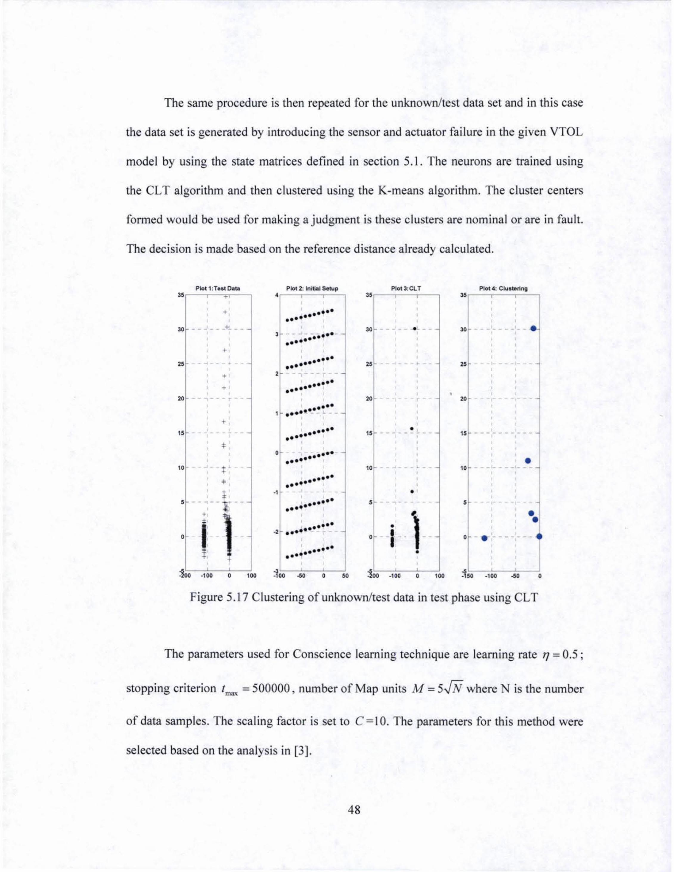
The same procedure is then repeated for the unknown/test data set and in this case

the data set is generated by introducing the sensor and actuator failure in the given VTOL

model by using the state matrices defined in section 5.1. The neurons are trained using

the CLT algorithm and then c lustered using the K-means algorithm. The cluster centers

formed would be used for making a judgment is these clusters are nominal or are in fa ult.

The deci sion is made based on the reference di stance already calculated .

ploll:nat Ditil

" +

30 ------ +'---

+

" •

+

20 - -- ~

"

10

•

:100 ·100

+

+ •

+ • 10 •

•

,

z

.. , .. , • ••••

.-' --.... --•••• ••••

..' •••• ••••

.' ••••• ••••

... ." , ....... . ~-- -

.' •••• ••••• o •••• •••• ."

.., . ,

."

•••• ••••

.. , •••••

•••• -2 ••••••• -

.. ••••• ••••

• ..

'" --

.. zo

Plot 3:CLT

, __ ... l __

, , " . , , , , , , , , , . ,

15 - - - - - - - - -

10

,

• . - 1-.

:ioo . 100

•

• , ,

'.

•

•

--

,

'00

30 --

zo

, ____ 1_-

, ,

, ,

, • 15 ----------•

, • 10 '----'---,

, , • •

o - .. ----,---

Figure 5.17 Clustering of unknown/test data in test phase using CL T

The parameters used for Conscience learning technique are learning rate 1] = 0.5 ;

stopping criterion 1m", = 500000 , number of Map units M = 5JN where N is the number

of data samples. The sca ling factor is set to C = 10. The parameters for this method were

selected based on the analysis in [3] .

48

.. -•• u 0

~ -5 •• r • >

-• >

" ~~~~-----r-----'------'------.~--~,:---~ .. fe'tentll

• CIu .....

30 -------- - ----~--------- ... -- -~

25 ----- - ....... --,--- - ,

"

"

10 • •

, ,

o

,

+

•

• • •

+

•

, , .'

- -

- --

~,,=--------.,~~~-------~~oC--------~~-------c .. ~-------o.,,=-------~oC-------~,o

Hori7.onla l "t lority

Figure 5.18 Test data set and corresponding cluster centers using CL T

" -~~~~~~~~::r:~------r--------'c--------,---------:--------~ • Nomin.l Data Clulters

"

"

• T.,t DUll CII,II~Ie" with 1'10 f' lIle r.'t D.UI Ciul"'rs In fau lt

- .... - -

,

,

- *'

- - ... ... -- .. - ... -- ...

15 -------~-------~----------------,-------~---

10 • ,

, ,

* , - ......... •• "'I , --._- .... --------- --,

• ~,~O ------~.,=~C-------~--------~1~O --------~ .. ~-------~~OC--------=O---------:,·O

Horizo ntal "tlocit)'

Figure 5.19 Identification of the faulty data clusters from the test data set

49

•

Figure 5.18 shows the test data plotted along with the cluster centers and these

wou ld be used for comparison with the nominal data clusters to make identification of the

cluster centers in fault. Figure 5.19 shows the test data clusters which are identified in

fau lt represented by a"'. As in the case of FSCL, using the CL T algorithm all the three

modes of operation were detected. The test data clusters that lie within the reference

distance from the training data clusters are termed as nominal and are shown in the

Figure 5.19. Figure 5.20 illustrates the test data clusters that were identified in fault

plotted along with the test data set. It gives an idea about the test data points that were in

fau lt. The performance of CL T in identifying the data points in faults is better than the

UCL technique as it avoids the dead units and identifies both the sensor and actuator

fai lure that were introduced.

-.. ruto.tII • Faulty elu_tlt,.

, 4 ,

30 ~ - -- - --- --- - -- ---1----- - -- .. - ----- - -I. _ ·et - --

+.

u -- ----T-------~--------~------- , -------~-

+ , " --- -- --·--------I--------r------------

o .-" , • - , ~ l' - ______________ ...! ______ .1-

-~ .-~

" >

, ,

10 ------------ ..... ----- -1--------. , ,

• :

, , , , , , ,. , , , , , , , ,

- - - --

5 - - - - - - --- - -- - - - -.- ~- t -~ -- - .,. -- --

+

o -------- ------------- - -- - -

12~' ----~.,~OO------~~~----~~~, ------~~'~----~.2~'------~,------~,,·

Horizontal velocity

Figure 5.20 Plot of test data and clusters detected in fault using CLT

50

5.5 Analysis using Self Organizing Maps (SOM)

Another improvement over the unsupervised competitive learning ru le was use of

neighborhood function while updating the winning neuron. Use of Self organi zing maps

allows the update of the winning neuron and its topological neighbors so that the dead

units (inactive neurons) can be avoided.

Plot 1: Nomi.,.1 Data ,

, • , I t+ ,

.+ + o ---- -..-'

·1 - - - - - -

Plot 2; lnitUlJ Setup

• , , , , ,

1 -----,-----

0.'

, ' " , , " ' ~ , , , ' , " ",' .. , , ' , , , , ,

" , , , , " , , , ,

0 -- . , • • • , ----

" , , , , , , , , , , , ,

, ,

" ..0.5 - - ~ •• - - - - -, , ,

.,

, , , "

, , , ,

, , , , , ,

~ ';;------CC----CC-____! . U;---C--____! -10 0 S _2 0 2

Plot J: SCM , ,

U - - - - - . - - - -, , ~

1 ---- ~-----, ... ~ , . ': O.S - .--- eZ.---­, , ,

.:: " o -- , - .,. .. "., ... .. .. '

~.5 -----! . ----;.. ' .. , • " -1 -----. ----

... "

-1.5 - - - - - - - - - -• , ,

Plot.; CIoJ'hI~ SOM , , •

,. •

. ' , .

o -------,--- -,

~, . • , ., - - - - - - .,. - - -,

, • .,.- - ---!-----! .u;----c:----c~____! .... 0 S ... -202

Figure 5.21 Clustering of nominal data in tra in ing phase using SOM

•

Figure 5.21 shows the training phase using the nominal data (+) based on SOM

algorithm. The clusters (. ) representing the trained neurons (. ) are shown in subplot 4

and are used as the baseline reference for fa ult identification. Figure 5.22 shows the

trained cluster centers and the nominal data set. Figure 5.23 shows the data clusters

formed using the unknown/test data set in the test phase by using SOM algorithm.

51

--

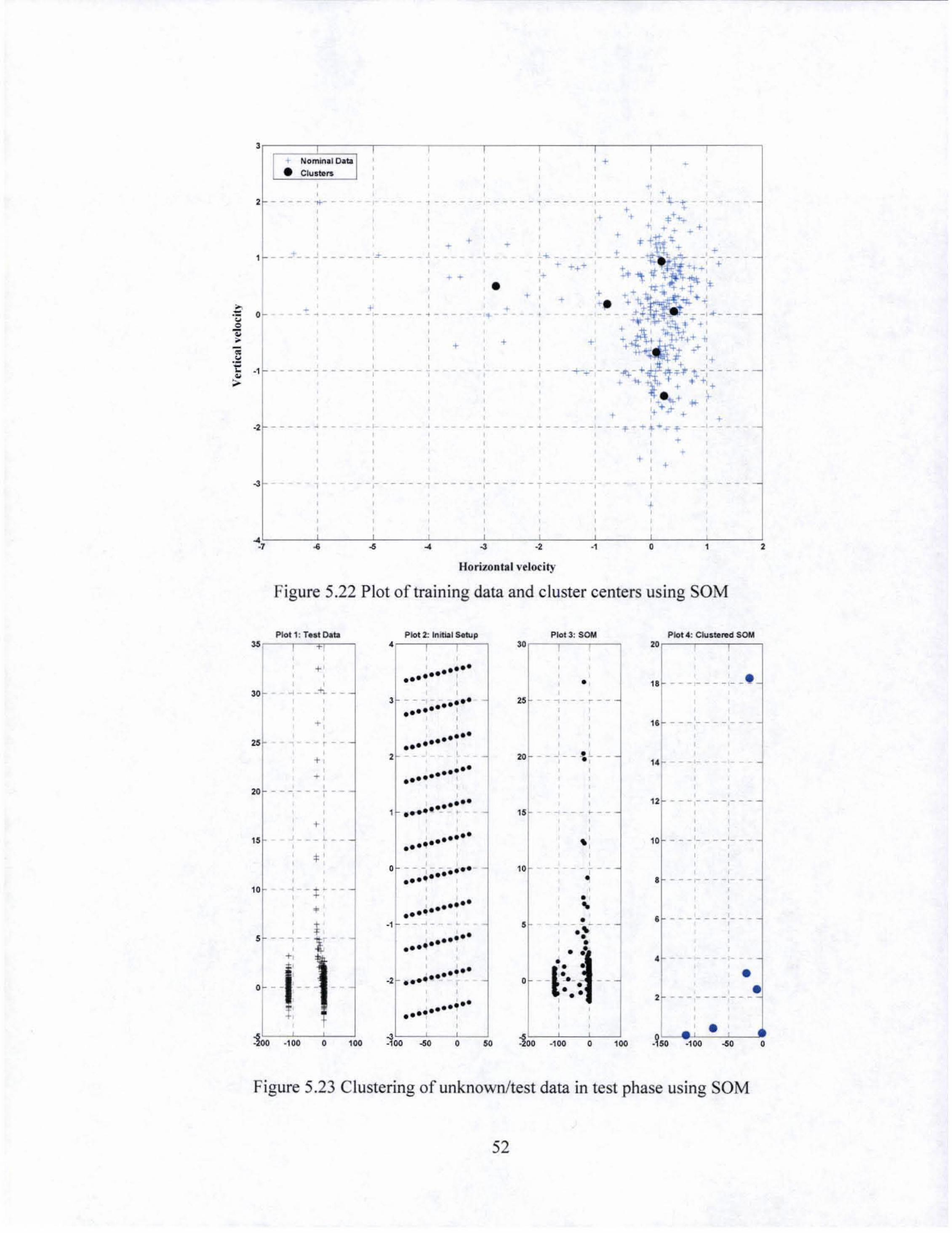
'ir=~~--~~~--~~~~ ,. Nom.,., o.tI + • Clulwl'$

, • , - --- - - - " ----T------,------T

, ---...--- ______ ~ ____ .I

.I

·1 --

, ,

------------- ~

, ---------- ---­•

,

++ • • • •

+ •

,

, + , , , , , ,

+ . , +

+ -------

• -. +

- - -~ ----t

+ --+

• 1 --, .... ----• , •

-2 --------- - ~-----.---------~--~ .. ~-----, , , , --------. ______ , ______ T ___ _

,

, • +

- - -- -

~7~------C~c-------C.c-------cC-------c~c-------C.,~------C.,c-------C,c--------,c--------;,

Horizontal vr lodty

Figure 5.22 Plot of training data and cluster centers using SOM

Plot 1: r .. t tAlb " r-- - .....,.-,

• 30

+

, +

20 ------

"

"

•

,

--,-,

+,

+ , _ l.. __

* +' -•

,

l

,

,

o

Plot 2: lnltl.ll SRlp , ••••

••••••• I , ,

- - - .' .. , •••••• I , ,

•••• ••••••• I

- -, , .. , .,.

••••• I

•••• .. , .-- - . ., ••••• •••• ,

• - - - - .­' ..... •••• ,

•••• •••• .., -1 - - - ~

., .. , .. ,

••••• .. , •••• ••••

••••• .... , ., , , 50

PlOI3: SCM "r--r--~......,

•

, 20 - ---'-- { ---

"

"

•

,

,

____ 0- __

,

, - - - - -• • ...

• --1:'-: • • , . .'00

, , , o ,00

PIot4: C)uste,.d SOM " ,----,---, ,

1&; - - - - - - - - - - -

1. - I

12 ---,----,--- -

" •

•

---,----,--, , ,

, -

-----------,

'r-, • • ---------- ~

• . \."'"0 -' .'"'00:-'-"+""-- 0

Figure 5.23 Clustering of unknown/test data in test phase using SOM

52

The parameters used for the Self Organizing Maps (SOM) algorithm are training

length I""" = 100000 ; learning rate 17 = 0.1. Figure 5.24 shows the test data plotted along

with the cluster centers and these would be used for comparison with the nominal data

clusters to make identification of the cluster centers in fault. Figure 5.25 shows the test

data clusters which are identified in fault represented by • *'. se of SOM algorithm

identified all three modes of operation. Data points correspond ing to both sensor and

actuator failu res were recognized. Even though SOM helps identifying the fai lure modes

that were introduced but it still does over-sampling of some low probability regions and

identifies data clusters where there are very few data points in a region. The test data

clusters that lie within the reference distance from the training data clusters are termed as

nominal and are shown in the Figure 5.26.

~Ir~~~-----------,------,-----,,-r----.------' - T •• to.UI I

"

"

. Cka ..... ( 1+ I , . -------<-----

T-----------~-, , ,

. ------~---~---------, ,

+,

T-------~------------

+

- ------------- - --• -____ ~ _______ l ____ _

, , , , ,

• , , , 10 - - - - - - - - - - - - - - .... ------------ + - ..

t ____ _ _

. --

• o , ,

-----,--------,- -

______ e _______ _ ,

+ , , , ,

-- -....,,- ,, --- ---r----.... - +-

. ~ J

--------,

1~~-----.~,OO~-----.~O~-----~+.-------~7.0~-----~+.O~----~O-------e20

Horizontal vtloci lY

Figure 5,24 Test data and corresponding cluster centers using SOM

53

'O~~.;=~N~.=m;I .. :JI;D='~~C~'"=';M=B===r==~------'-'----------~'----------:', ----------:-, --------~

"

• Test Data elusUors with no f.ult ....

'" * T .. t D.ta c:lntlr1l in f,ult

, -----_._----------, - -- --- - -: - - - - - - - - - - - - - - - -

10 -~ - - - - ------T----------- --•• " 5! • >

•• 1: •

, ,

, > 5 -------~------ ., I-------~ ________ t-------

» -•• " o

i -•• J: ~

o - * ---- - -------~­, •

"" •• - - - - --. - - - - - - . -- - - --

! ,

~,~O--------.~l00~--------.~Oo---------~~OC--------c~~O----------~,Oo---------~O--------~2·0

Horizontal vtlocity

Figure 5.25 Detection of data clusters in fault using SOM

t Te.tO.tI • Fau lty CIu.ters

, J.O ------- ~ --------

"

20 -------T-------~--

15 - - - - - - - -, ..

, , , ------------,-

+

o

,

---+-------~---~-----------

, , +

----~--------,-------

•

• , ----------------------,

• +

-----------'---

--------- - -~--------,-+ , • , , ~ ...., ..

"--.--,-------

- . ,.

,

~~.-------~.,*OO;-------~.~O--------~ .. ;--------~~--------.~~;--------;O---------;2'O

Horizontal vtlotity

Figure 5.26 Test data and clusters detected in fault using SOM

54

5.6 Performance comparison of algorithms

The performance of different algorithms was tested using the data set that was

generated using the VTOL aircraft model. As di scussed earlier there were three differen~

modes of operation i.e. nominal mode, sensor failure and actuator failure . The data was

generated based on the system matrices defined in Table 5.1. Figure 5.27 illustrates the

data set used for test phase and shows the data points associated with different modes of

operation.

112 r;=::;o::;:::~::;-------,--------,-----r---,------, NominlilOatil I +

of" Sensor Fault ~tullt(lr Folult

, '1 0 ------ - ----,

'01 , , , , , ,

,

, , , ,

+ ------ -- --- ------

+ •

------------------------,-------

~ ,0< • ----------~-------- - --- -·S 1 ~ • , •

• > '04 -----~------~-----------------~ , , , ,

102 -------, , , ,

100 ------- ------- -

,

-, , t.' ,

• - - - .. - - - - - - .+. - - - - - - - - - - - - - - -L + I

'~ + .... +' • .

t

, __ .., ____ _ z"' ------

.. ~--~-----~------+.-----~~-----+.~----~----~ .~ D 20 '0 M 80 100 1N

HorizoruI ... IcIo~

Figure 5.27 Plot of data set used for test phase showing data points associated with different modes

Now as shown by the results obtained by using UCL algorithms for training and

test phases, the UCL algorithm is not able to detect the cluster of data points due to the

55

sensor fault. The occurrence of dead units or inactive neurons in the test phase using the

VeL algorithm leads to poor assignment of the cluster centers and hence the FDI scheme

is not able to detect the different fault modes that were introduced in the test data set.

VCL algorithm thus provides under-sampling of the high probability regions and over­

sampling of the low probability regions. The performance of VCL algorithm for

clustering and classification purposes is relatively poor as compared to the improvements

based on equiprobable mapping and SOM.

To overcome the problem of VCL algorithm being unable to identify all fault

modes due to occurrence of dead· units the FSCL and CL T algorithms were developed.

From Figures 5.13 and 5.14 it is clear that the F~CL algorithm provides a good clustering

and classification of the nominal and failure modes. FSCL algorithm was able to identifY

the sensor and actuator failures and the nominal mode of operation.

Similarly from Figures 5.19 and 5.20 it is evident that the CLT algorithm provides

an equiprobabilistic map formation and hence avoids the occurrence of dead units or

inactive neurons. The trained neurons using this algorithm provide a good representation

of the input data set" and hence the FDI scheme is able to identifY both the sensor and

actuator failure that were introduced. Thus the performance of FSCL and CL T algorithm

is better than the VCL algorithm as the dead units are avoided.

The SOM algorithm uses a neighborhood function for training the neurons and as

discussed earlier, instead of the winner takes all strategy the weights of the neighboring

neurons of the winning neuron are also updated. Hence this approach also helps in

avoiding the dead units and provides a better clustering and classification appro~ch for

FDI. Figure 5.25 and 5.26 illustrate the performance of the SOM algorithm in detecting

56

and identifying the fault modes. The SOM algorithm is also able to correctly detect and

identify both the sensor and the actuator faults that were introduced. However the

performance of SOM is not at par with the FSCL and CL T algorithms because it still

does over-sampling of some low probability regions. When the neighborhood range is too

rapidly decreased during the SOM learning phase, dead units can still occur in practice.

Use of Bauer Der and Herrmann (BDH) and Kernel based Maximum Entropy learning

(k-MER) algorithms provide an improvement over SOM and" are referred for

investigation under future work in the section 6.2.

,

<,

57

•

•

CHAPTER 6

CONCLUSIONS

6.1 Summary

The research presented in this thesis gives us an understanding of Condition

Based Maintenance (CBM) based on the data driven approach for Fault detection and

Identification (FOI) in control systems. The simulations presented in this thesis show that jo

competitive learning based techniques can be used as an effective approach for the FDI

and can detect and identify the failure scenarios in control systems.

The use of Unsupervised Competitive Learning (UCL), equiprobable mapping

techniques like Frequency Sensitive Competitive Learning (FSCL), Conscience Learning

Technique (CLT) and topographic mapping technique like Self Organizing Maps (SOM)

were applied for the FOI scheme and the performance of these algorithms for the FDI

was demonstrated. The FSCL, CL T and SOM based FOI schemes provided a better FDI

scheme as compared to the VCL approach as the dead units (inactive neurons) that

occurred in the VCL approach were eliminated. K-means algorithm was used for

clustering the neurons that were trained using the above mentioned algorithms. We used a

heuristic approach to come up with the approximate number of cl usters to be used for the

K-means algorithm so that we get a good clustering analysis of the given data set.

Effectiveness of the developed algorithms is tested using the data available from a

Vertical Take off and Landing (VTOL) aircraft model.

Simulation results based on the data available from the VTOL aircraft model

illustrated that the use of equiprobable mapping in case of FSCL and CL T and

58

neighborhood function in case of SOM would provide a more robust and accurate FDI

scheme as compared to the VCL based approach. The sensor and actuator faults that were

introduced in the VTOL model were identified by these schemes.

6.2 Future work

Contrary to what was originally assumed by Kohonen [4], the weight density of

the trained neurons at convergence also termed as the (inverse of the) magnification

factor in this context, is not a linear function of the input density p(v) where v E!Rd

represent the input data vectors. Thus the weight density achieved by SOM was not a

linear function of the input density and is given by:

I

1+2. pew,) oc p ~ (v) (6.2.1)

Hence the neurons of the map in case of SOM will not be active with equal

probabilities (i.e. the map is not equiprobabilistic). Thus in the cases where the clusters

formed are not clearly separated the SOM algorithm would tend to oversample the low

probability· regions and undersample the high probability regions in the input

distributions.

To overcome this difficulty other algorithms such as Bauer Der and Herrmann

(BDH) algorithm and Kernel based Maximum Entropy learning (k-MER) can be used.

The idea behind the approach is to build a map with a learning rule that maximizes

information theoretic entropy directly. As a result the map will transfer maximum amount

of information available about the distribution from which it receives the input and a

more faithful representation can be made.

59

REFERENCES

[I] D. C. Swanson, "A general prognostic tracking algorithm for predictive

maintenance", in IEEE Aerospace Conference Proceedings., vol. 6, March 2001, pp.

2971-2977.

[2] J. Luo., M. Namburu, and et ai, "Model-based Prognostic Techniques ", IEEE

Systems Readiness Technology Conference Proceedings, September 2003, pp. 330-

340.

..

[3] Van. Hulle, M.M.; "Faithful Representations and Topographic maps -from Distortion

to Information 'Based SeljOrganization", John Willey & Sons 2000.

[4] T. Kohonen, "Self-Organizing Maps" Second Edition, Springer, 1997.

[5] Zhang, Y.M., and Li, X.R., "Deteetio'! and diagnosis of sensor and actuator failures

1!sing IMM estimator ". IEEE Transactions on Aerospace and Electronic Systems, vol.

34, No.4, 1998, pp. 1293-1313.

[6] Zhang, Y., and Jin, J., "Integrated Active' Fault tolerant Cont/ol Using IMM

Approach ", IEEE Transactions on Aerospace and Electronic Systems, vol.37, No.4,

2001, pp. 1221-1235.

[7] S. Haykin, "Neural Networks -A Comprehensive Foundation", Prentice Hall 1999.

60 •

[8] Grossberg, S., "Adaptive pattern classification and universal recording: I Parallel

development and codingofneuralJeature detectors", Biol. Cybem., 23, pp. 121-134.

[9] Rumelhart, D.E., and Zipser, D. "Feature discovery by competitive learning",

Cognitive Science, 9, pp. 75-112.

[10] DeSieno, D., "Adding a conscience to competitive learning", IEEE Int. Conf. on

Neural Networks (San Diego), vol. I, pp. 117-124.

[II] Van Hulle, M.M., Martinez, D., "On an unsupervised learning rule Jor scalar

quantizationJollowing the maximum entropy principle", Neural Computations., 5, pp.

939-953.

[12] Van den Bout, D.E., and Miller lJI, T.K., "TInMANN: The Integer Markovian

Artificial Neural Network:', Proc. Int. Joint Conf. on Neural Networks (IJCNN89),

Englewood Cliffs, NJ: Erlbaum, pp.1I205-11211.

[13] Ahalt, S.c., Krishnamurthy, A.K., Chen, P., and Melton, D.E., "Competitive

learning algorithmsJor vector quantization", Neural Networks, 3, 277-290.

[14] Vesanto, J. and Alhoniemi, E., "Clustering of the Se/.fOrganizing Maps", IEEE

transactions on Neural Netw~rks, vol. II, no. 3, May 2000.

61

[IS] Bezdek, J.e. and Pal, S.K., "Fuzzy models for pattern recognition: Methods that

search for structures in the data", New York: IEEE 1992.

[16] Mclahlan, GJ. and Basford, K.E., "Mixture Models: Inference and Applications to

clustering", New York: Marcel Dekker, vol. 84, 1987.

[17] Boudaillier, E. and Hebrail, G., "Interactive interpretation of hierarchical

clustering" Intell. Data Anal., vol. 2, no. 3, 1998.

[18] Buhmann, J. and Kuhnel, H., "Complexity optimized data clustering by competitive

" neural networks", Neural Compu!., vol. '5, no. 3, pp. 75-88, May 1993.

[19] Bezdek, J.C., "Some new indices of cluster validity", IEEE Trans. Syst., Man,

Cybem. B, vol. 28, pp. 301-315,1998.

[20] Milligan, G.W. and Cooper, M.C., "An examination of procedures for determining

the number of clusters in a data set", Psychometrika, vol. 50, no. 2, pp 159-179, June

1985.

[21] Jain, A.K. and Dubes, R.e., "Algorithmsfor clustering data", Prentice Hall 1988.

62