University of Groningen Harmonization by simulation Nowok ...
122
University of Groningen Harmonization by simulation Nowok, Beata IMPORTANT NOTE: You are advised to consult the publisher's version (publisher's PDF) if you wish to cite from it. Please check the document version below. Document Version Publisher's PDF, also known as Version of record Publication date: 2010 Link to publication in University of Groningen/UMCG research database Citation for published version (APA): Nowok, B. (2010). Harmonization by simulation: a contribution to comparable international migration statistics in Europe. [s.n.]. Copyright Other than for strictly personal use, it is not permitted to download or to forward/distribute the text or part of it without the consent of the author(s) and/or copyright holder(s), unless the work is under an open content license (like Creative Commons). The publication may also be distributed here under the terms of Article 25fa of the Dutch Copyright Act, indicated by the “Taverne” license. More information can be found on the University of Groningen website: https://www.rug.nl/library/open-access/self-archiving-pure/taverne- amendment. Take-down policy If you believe that this document breaches copyright please contact us providing details, and we will remove access to the work immediately and investigate your claim. Downloaded from the University of Groningen/UMCG research database (Pure): http://www.rug.nl/research/portal. For technical reasons the number of authors shown on this cover page is limited to 10 maximum. Download date: 14-02-2022
Transcript of University of Groningen Harmonization by simulation Nowok ...

University of Groningen
Harmonization by simulationNowok, Beata
IMPORTANT NOTE: You are advised to consult the publisher's version (publisher's PDF) if you wish to cite fromit. Please check the document version below.
Document VersionPublisher's PDF, also known as Version of record
Publication date:2010
Link to publication in University of Groningen/UMCG research database
Citation for published version (APA):Nowok, B. (2010). Harmonization by simulation: a contribution to comparable international migrationstatistics in Europe. [s.n.].
CopyrightOther than for strictly personal use, it is not permitted to download or to forward/distribute the text or part of it without the consent of theauthor(s) and/or copyright holder(s), unless the work is under an open content license (like Creative Commons).
The publication may also be distributed here under the terms of Article 25fa of the Dutch Copyright Act, indicated by the “Taverne” license.More information can be found on the University of Groningen website: https://www.rug.nl/library/open-access/self-archiving-pure/taverne-amendment.
Take-down policyIf you believe that this document breaches copyright please contact us providing details, and we will remove access to the work immediatelyand investigate your claim.
Downloaded from the University of Groningen/UMCG research database (Pure): http://www.rug.nl/research/portal. For technical reasons thenumber of authors shown on this cover page is limited to 10 maximum.
Download date: 14-02-2022

HARMONIZATION BY SIMULATION

ISBN 978 90 367 4550 5 Printed by Rozenberg Publishers, Amsterdam © Beata Nowok, 2010 All rights reserved. Save exceptions stated by the law, no part of this publication may be reproduced, stored in a retrieval system of any nature, or transmitted in any form or by any means, electronic, mechanical, photocopying, recording or otherwise, included a complete or partial transcription, without the prior written permission of the proprietor.

Rijksuniversiteit Groningen
Harmonization by Simulation A Contribution to Comparable International
Migration Statistics in Europe
Proefschrift
ter verkrijging van het doctoraat in de Ruimtelijke Wetenschappen
aan de Rijksuniversiteit Groningen op gezag van de
Rector Magnificus, dr. F. Zwarts, in het openbaar te verdedigen op
donderdag 28 oktober 2010 om 13.15 uur
door
Beata Nowok
geboren op 6 september 1978 te Cieszyn, Polen

Promotor: Prof. dr. ir. F.J. Willekens
Beoordelingscommissie: Prof. dr. C.H. Mulder Prof. dr. P.H. Rees Prof. dr. L.J.G. van Wissen

Table of contents
List of tables List of figures Preface
1. Introduction ............................................................................................................. 1 1.1. Background: migration counts ......................................................................... 1 1.2. Recent research on harmonization of migration statistics ................................ 2 1.3. Outline of the book........................................................................................... 4 References ................................................................................................................. 7
2. Progress in counting international migrations in Europe, 1998-2007 ................ 9 2.1. Introduction ...................................................................................................... 9 2.2. Data availability.............................................................................................. 11 2.3. Graphical comparison of migration data ........................................................ 13 2.4. Measuring agreement between migration matrices ........................................ 16 2.5. Comparison results ......................................................................................... 19
2.5.1. Comprehensive agreement measures ................................................. 19 2.5.2. The pattern of changes in relative absolute differences ..................... 22 2.5.3. The nature of changes in relative absolute differences:
remarks about future research ............................................................ 26 2.6. Conclusions .................................................................................................... 28 References ............................................................................................................... 29 Appendix ................................................................................................................. 31
3. A probabilistic framework for harmonization of migration statistics.............. 33 3.1. Introduction .................................................................................................... 34 3.2. Migration process ........................................................................................... 36 3.3. Observation plans and measures .................................................................... 39 3.4. Indicators of migration process ...................................................................... 41 3.5. Conclusions .................................................................................................... 49 References ............................................................................................................... 50
4. Reconciliation of various event-approach migration measures: insights from microsimulation of origin-destination specific flows .......................................... 55 4.1. Introduction .................................................................................................... 55 4.2. Measures of migration: from biographies to statistics ................................... 57
4.3. Microsimulation of origin-destination flows...................................................63 4.4. Reconciling different migration measures ......................................................64 4.5. Conclusions .....................................................................................................70 References ................................................................................................................71 Appendix ..................................................................................................................73
5. Reconciliation of migration measures by linking migration flows and population stocks ....................................................................................................75 5.1. Introduction .....................................................................................................75 5.2. Model considerations ......................................................................................76 5.3. The maximum likelihood estimation of relocation intensities ........................80 5.4. Conclusions .....................................................................................................84 References ................................................................................................................84
6. Analysis of data on origin-destination migration dynamics with R ..................87 6.1. Introduction .....................................................................................................87 6.2. Simulation .......................................................................................................88 6.3. Migration measures .........................................................................................90 6.4. Plotting results.................................................................................................92 6.5. Conclusions .....................................................................................................94 References ................................................................................................................95 Appendix ..................................................................................................................96
7. Conclusions ...........................................................................................................103
Samenvatting ..............................................................................................................107

List of tables
Table 2.1 Percentage of origin-destination flows with complete, partial or no data, 1998-2007 ..13 Table 2.2 Percentage of flows with complete data for which immigration and emigration data
are equal (IMij=EMij), immigration data are higher than emigration data (IMij>EMij) and immigration data are lower than emigration data (IMij<EMij), 1998-2007 .............16
Table 2.3 Measures of similarity between immigration and emigration matrix, 1998-2007......................................................................................................................20
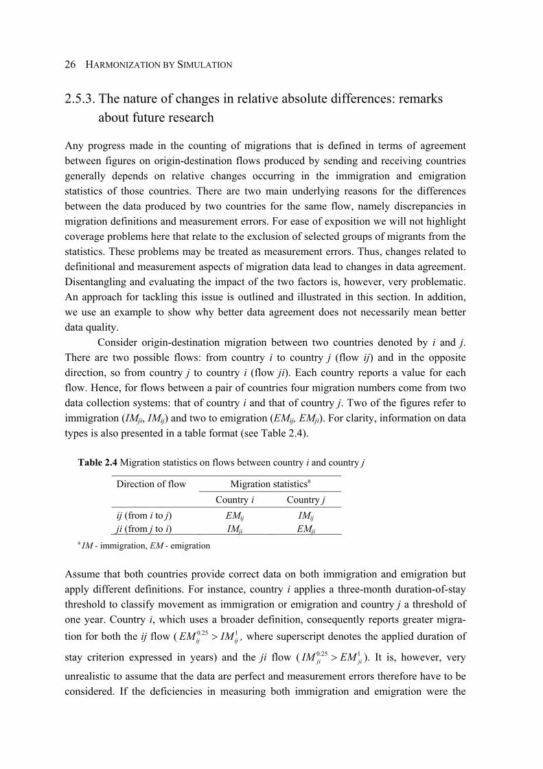
Table 2.4 Migration statistics on flows between country i and country j ......................................26 Table 2.5 Immigration matrix: migration flows between ten EU countries according to the
receiving countries in 2007............................................................................................31 Table 2.6 Emigration matrix: migration flows between ten EU countries according to the
sending countries in 2007 ..............................................................................................31
Table 3.1 Main types of migration data.........................................................................................40
Table 4.1 Migration definitions with different types of duration conditions.................................60 Table 4.2 Individual relocation history expressed in duration variables and its contribution to
different origin-destination migration measures produced by countries A, B and C ....73
Table 5.1 Country-to-country migrations in 2006 as reported by the countries of destination .....83 Table 5.2 Average population number in 2006 .............................................................................83 Table 5.3 Maximum likelihood estimates of origin-destination relocation intensities in 2006.....83 Table 5.4 Expected number of origin-destination relocations in 2006 ..........................................83

List of figures
Figure 2.1 Scatter plot of origin-destination migration flows in EU-25 as reported by origin (EMij) and destination (IMij) country, 1999-2007, with line of equality; logarithmic scale ...............................................................................................................................14
Figure 2.2 Scatter plot of origin-destination migration flows in EU-25 from Germany (DE), Poland (PL) and Sweden (SE) as reported by origin (EMij) and destination (IMij) country, 1999-2007; logarithmic scale ..........................................................................15
Figure 2.3 Measures of similarity between immigration and emigration matrix, 1998-2007.........21 Figure 2.4 Histograms of relative absolute difference (RADij) for the period 1998-2007 by
migration volume: [0, 20), [20, 400), [400, 5000) and [5000, Inf). The cut points are derived from the 1st, 5th and 9th deciles of migration volume ...............................22
Figure 2.5 Empirical cumulative distribution functions of relative absolute difference (RADij) between immigration and emigration figures; 1999, 2003 and 2007 ............................23
Figure 2.6 Histogram of relative absolute difference (RADij) between immigration and emigration figures; 1999, 2003 and 2007 ......................................................................23
Figure 2.7 Observed and estimated proportions of different categories of RADij; 2007.................24 Figure 2.8 One-year transitions of relative absolute difference (RADij); 1998-2007. Grey
dashed lines indicate six categories of RADij.................................................................25
Figure 3.1 Ratio of conditional migration measures for various lengths of duration threshold to conditional measures for one year; left panel: conditional migrations, right panel: conditional migrants ......................................................................................................43
Figure 3.2 Conditional migrations per conditional migrant for the same duration tm = tM; annual data .....................................................................................................................44
Figure 3.3 Ratio of conditional migrations to conditional migrants, for various durations up to one year and intensity λ=0.2; solid line is a contour line of value one; dashed line is a line of equality of tm and tM .........................................................................................45
Figure 3.4 Expected number (per individual) of transitions over intervals of different lengths for selected intensities....................................................................................................47
Figure 3.5 Ratio of transitions over an interval of different lengths to transitions over one year...48 Figure 3.6 Expected number (per individual) of conditional migrations for one year and
transitions over one year with and without restriction on minimum duration of residence ........................................................................................................................49
Figure 4.1 Relocation path of individual k between three countries (A, B and C) over five years...............................................................................................................................58
Figure 4.2 Relocation path of individual k between countries A, B and C over five years observed in different countries of reference indicated in brackets ................................59
Figure 4.3 Contribution of individual’s relocations to various migration measures (Ia, Ib, IIa, IIb, II, IV) by country A, B and C; vertical lines with arrows indicate relocations that are counted as migrations by respective countries of reference............................. 60
Figure 4.4 Proportion of total relocations in the system that satisfy a particular duration criterion applied in measure (III); exponential and Weibull duration model; two sets of origin-destination relocation intensities: λij and 0.1λij....................................... 66
Figure 4.5 Shares of relocations that fulfil duration criteria of different lengths for measure (III); exponential and Weibull duration model; two sets of origin-destination relocation intensities: λij and 0.1λij ............................................................................... 66
Figure 4.6 Ratio of different migration measures, (Ia, Ib, IIb), to measure (III) for two sets of origin-destination relocation intensities: λij and 0.1λij; left panel: exponential duration model, right panel: Weibull duration model................................................... 67
Figure 4.7 Migrations from countries A and C to country B according to measures IIa, IIb and III with different lengths of duration criterion, as observed by origin and destination countries; expressed as a proportion of the number of respective relocations; (a) exponential duration model, (b) Weibull duration model.................... 68
Figure 4.8 Ratio of immigration to emigration number according to measures IIb and III for origin-destination specific flows; left panel: exponential duration model, right panel: Weibull duration model ..................................................................................... 69
Figure 4.9 Emigration rates estimated from simulated relocations counted as migrations according to measure (III); left panel: exponential duration model, right panel: Weibull duration model, estimation under the assumption of constant hazard rates.... 70
Figure 6.1 Number of origin-destination specific migrations (solid line) and transitions (dashed line) for various durations up to one year........................................................ 93
Figure 6.2 Person-years of residence (black bars) and person-years of actual stay in country of residence (grey bars) for various duration criteria in migration definition; country = 2, year = 10................................................................................................... 94
Preface
This is a book about international migration data, and according to most definitions I became an international migrant on the way to the final sentence. I do not know if the road I chose was the best one to take. I do know, however, that thanks to fate or pure chance I had the privilege of staying in places where both well-established and promising future demographers were ready to share their knowledge and experience. Let me retrace my steps back to the first demographer I met. In 2006, somewhat to my surprise, I was granted the opportunity of becoming a PhD candidate at the Population Research Centre (PRC) at the University of Groningen, the Netherlands. I would not have missed this opportunity for the world. I spent my three-year research period at the Netherlands Interdisciplinary Demographic Institute (NIDI) in the Hague. It was a very pleasant working environment with friendly colleagues who were ready to offer help of any kind. Thank you all. First and foremost, however, I would particularly like to thank Frans Willekens for his guidance, for many inspiring discussions, for support and encouragement, and for every single challenge he set me. This was an invaluable experience. Frans had already become my mentor in September 2005. I came to the Max Planck Institute for Demographic Research in Rostock, Germany as a NIDI fellow to attend the European Doctoral School of Demography (EDSD). Here, in a stimulating international environment surrounded by dedicated and enthusiastic demographers I acquired not only demographic knowledge but also a group of friends. It is difficult to put into words exactly how much I enjoyed the camaraderie of the first EDSD cohort. I was also lucky enough to have the very understanding company of Ania. Prior to this, I gained experience in Poland at the Central European Forum for Migration and Population Research (CEFMR) in Warsaw, where I got into demographic research and where I first encountered the field of harmonizing statistics on international migration. The idea for my PhD research originated here as well. I am greatly indebted to Dorota Kupiszewska and Marek Kupiszewski for their guidance and for providing a friendly and supportive atmosphere. My gratitude also goes to Michel Poulain together with all the other European partners from the THESIM project in which I took part. The Warsaw School of Economics is where I heard the first story about demo-graphics. An exceptional man of deep humanity told it: Jerzy Zdzisław Holzer. His great voice still echoes, guiding one in the right direction, even though he has passed on. That is how my story unfolded. However, some other places are of special signifi-cance to me and they have not yet been marked on my map. They include Southampton and Leeds, where I attended migration workshops and summer school respectively. I am

particularly grateful to Phil Rees for sharing his insights and expertise. My next destination is St Andrews where I will again spend a period of time, taking with me good memories of the people I have met on my way. Some have been a considerable influence on me as a researcher and as a person. Some just smiled at me. Thank you to all of you. Many deserve special thanks and I hope they know who they are. Extra special thanks go to all my family and friends, wherever they are. They are always very close even if geography separates us.
11
1. Introduction
1.1. Background: migration counts
How many people migrate internationally every year? Is there a simple answer to this seemingly straightforward question or have we already lost count? Counting is a trivial task, provided two essential prerequisites are met. First, there must be agreement on what to count. Second, the right tools must be in place. In the case of international migration, both of these aspects are highly problematic. Many countries do not have a data collection system for international migration or do not process and publish the data gathered. Countries that prepare and release migration numbers use diverse concepts and measures of migration. Furthermore, the accuracy of the counting process itself is very often unsatisfactory. Even if we aim to count only the legal migrations, many migratory events, especially emigrations, take place unnoticed. We are therefore faced with a common problem of data quality. Migration statistics are relatively weak in many countries and an estimate of international migration at a global level is at best very rough.
At the same time, international migration is a highly topical issue of concern to an increasing number of countries. It draws the attention of policymakers, scholars, the media and the general public. Sensitive topics such as the management of migration and the integration of migrants are consistently in the headlines. It is becoming increasingly important to have sound data on international migration and migrants that can form the basis of a reasoned discussion. Solid statistical evidence is essential for gaining an understanding of the phenomenon of international migration and its impact on various areas of social and economic life. This knowledge base should assist in the development of effective policies that benefit migrants, the countries they leave and those they move to. In today’s globalized world, migration policy is more than just a national concern that can be developed in isolation. In order to develop a common migration policy, countries need to

HARMONIZATION BY SIMULATION
2
coordinate the counting process of migrants and monitor trends and patterns of interna-tional migration in a reliable manner.
The demand for information about international migration certainly extends beyond counting migration flows. Nonetheless, the controversy begins with these basic figures. The national statistical institutes provide data on immigration and emigration, but in many countries few believe the numbers to be exact. The general public in particular tends to believe that the statistics understate the reality. Additional unofficial estimates are pro-duced, which are claimed to be more reliable. The media quotes them and politicians use them for advocacy, even though many of the figures are at best educated guesses.
There is a simple method for cross-checking statistics on migration flows. Emigra-tion data from one country can be matched against immigration data in receiving countries. Country A’s figures for immigration from country B should be equal to country B’s figures for emigration to country A. They usually differ, sometimes considerably, from each other. This is not just because emigration is more difficult to measure than immigration. The measurement error varies between countries because the quality of their data collection systems differs. Furthermore, the definition of migration is of fundamental importance. If countries define migration differently, then accurate data on emigration and immigration will not match.
1.2. Recent research on harmonization of migration statistics
It has been recognized for years that there are deficiencies in official statistics on interna-tional migration flows. At the same time, much of the research that has been carried out has not paid sufficient attention to the reliability of the migration numbers and the details of the migration definitions used by different countries. Other studies have found that the available data are inadequate for a proper analysis of migration issues. It means that we may often be faced with either erroneous or partial results. Over the years only limited improvements have been made to the data quality. Nevertheless, some important steps were recently taken at the European Union level that should help provide better informa-tion on migration flows. In August 2007, the new Regulation of the European Parliament and of the Council on Community statistics on migration and international protection came into force (European Commission, 2007). Starting from the reference year 2009, the Regulation obliges member states to provide migration statistics that comply with a harmonized definition. The definition corresponds to that of long-term migration proposed by the United Nations in the recommendation on statistics of international migration (United Nations, 1998: Box 1). This legal basis for the collection and compilation of migration

INTRODUCTION
3
statistics that the Regulation sets out would seem to be essential in the harmonization process in view of the fact that the UN recommendation has been generally ignored by most countries. Most figures on international migration are by-products of data gathered for reasons other than the measurement of the flows of migrants. The definitions underly-ing the official statistics on immigration and emigration differ considerably between the EU member states. In addition, there is not usually the appropriate metadata to accompany the migration numbers. Acknowledging the need for better information on migration statistics and national data sources and acknowledging possibilities for improvement, the European Commission founded two relevant research projects under the Sixth Framework Programme, namely THESIM (http://www.uclouvain.be/en-7823.html) and PROMINSTAT (http://www. prominstat.eu). THESIM is an acronym for Towards Harmonised European Statistics on International Migration and the knowledge provided by the project is essential if progress is to be made towards providing better data on migration. One of the main objectives of the project was to investigate the current functioning of migration statistics in the 25 EU countries. The members of the THESIM team used a unique source of information. They met with national experts and the authorities involved in the statistics production process in each country. The resulting book (Poulain et al., 2006) constitutes an invaluable source of detailed information on collecting and compiling migration data in the 25 EU countries. It presents the state of the art as of 2005. The PROMINSTAT research project – Promoting Comparative Quantitative Research in the Field of Migration and Integration in Europe – has supplied complementary information. One of the main results is a comprehensive inventory of the statistical and administrative datasets relevant to the study of migration that are collected in 27 European countries. It is available as an online database (http://www.prominstat.eu/prominstat/database) with a potential wide application in the interdisciplinary field of migration studies. Some deficiencies present in migration statistics that are described within the two projects mentioned above may be tackled using modelling techniques. The need for such an approach has been recognized by EU policymakers. The new Regulation on Community statistics on migration and international protection provides the possibility of using estimation methods to adapt statistics that are based on national definitions so that they comply with the harmonized definition. In addition, Eurostat funded the MIMOSA project – Migration Modelling for Statistical Analyses (http://mimosa.gedap.be/) – that aimed to develop a method for reconciling the differences in international migration statistics in European countries. The project produced, among other outputs, estimates of the origin-destination specific migration flows between 31 European countries. The authors of the methodology claim that harmonizing the reported data was the most difficult task they faced (De Beer et al., 2009). Using origin-destination specific flows as reported by sending and receiving countries, they came up with a set of adjustment factors for both immigration and emigration figures that minimize the differences between the two available datasets.

HARMONIZATION BY SIMULATION
4
The correction factors were obtained from a constrained optimization procedure. In principle, this is the same approach to the harmonization of international migration data as that suggested by Poulain (1993) and later revised by Poulain and Dal (2008). A recent study by Abel (2009) provides a useful overview of the method and explores various alternative distance measures and constraint functions. Note that these methods do not provide answers about the linkage of one measure of migration to another. The values of the correction factors indicate the level of discrepancies between figures reported by different countries, but the definitional problems only cause some of the differences. Scientific research that aims to obtain an overall and consistent picture of the migration patterns occurring within Europe will continue within the NORFACE Research Programme on Migration. The programme has granted funding to the IMEM project – Integrated Modelling of European Migration (http://www.norface-migration.org/current projectdetail.php?proj=3) – and this project will seek to apply Bayesian methods in order to harmonize and correct for inadequacies in the available migration data.
1.3. Outline of the book
Continuing to improve the quality of data on migration flows remains a key task in migration research. A major challenge in this regard that deserves a great deal of attention is the impact of the definition of migration on the resulting migration numbers. The ultimate goal is to develop a simple and systematic method that will enable the reconcilia-tion of the definitional differences in the available data. A vital prerequisite for the harmonization of migration statistics is, however, a thorough understanding of these data. The research presented in this thesis is a further step towards harmonized data on migration flows. A simulation approach is used to facilitate this progress. A starting point and at the same time a focal point of the study is the general notion that all migration measures are different observations of the same underlying process. It is crucial, therefore, to make a link between the process and the available statistics on migration flows. Knowledge of the parameters of the process that is generating the data represents a basis from which figures on migration can be derived according to various definitions. This idea represents a novel approach to reconciling differences in migration measures. As an illustration we have selected measures that are prevalent in European statistical practice. Limitations of the available data meant that much of the analysis was carried out using simulated mobility histories of individuals. A great advantage of this microsimulation approach is complete control over the counting of predefined migration events. The migration measures derived for the whole virtual population are accurate, and discrepancies between various measures on migration flows result from differences in definition only. Microsimulation and all the necessary calculations were carried out in R.

INTRODUCTION
5
The book consists of seven chapters, including the present introductory Chapter 1 and the concluding Chapter 7. The remaining chapters are self-contained articles that have either been submitted or will be submitted for publication in scholarly journals. They can be read separately, but equally any overlap between chapters has been kept to a minimum. The book as a whole provides the comprehensive picture of migration statistics that is necessary if one wishes to understand their complexity and adjust them to a harmonized definition. The overview below summarizes the main contents and purposes of Chapters 2-6. Chapter 2 evaluates the progress made over a decade (1998-2007) in counting international migrations in 25 European Union countries. We look at the availability and comparability of the origin-destination specific statistics on international migration flows provided by sending and receiving countries. As regards comparability, our main objective was to assess the overall agreement between two available datasets referring to the same flows but provided by origin and destination countries respectively. We investigated various comprehensive measures in order to find the one that was best suited to this purpose. To the best of our knowledge, comparisons of origin-destination migration statistics have so far only been conducted at the level of a single country-to-country flow. Moreover, a systematic assessment of changes in data similarity over time is lacking. Despite the difficulties that still exist in measuring migration we would expect a general improvement. For readers unfamiliar with the inconsistencies in statistics on migration flows produced by different countries, this chapter provides a good indication of the scale of the problem. Others may find some useful tools here for monitoring future progress in data comparability. Chapter 3 proposes a novel approach to the harmonization of statistics on interna-tional migration flows. We present a theoretical probabilistic framework that is able to accommodate various available migration flow statistics. Different migration measures represent observations of the same continuous-time migration process. The differences depend on how migration is defined, the way the data are collected and how the statistics are produced and published. We introduce the key concepts of migration statistics using the simplest duration model, namely an exponential distribution. The main focus is on the time criterion used in migration definition. This refers to the duration of stay following relocation, which is specified very differently by different countries and which constitutes the main source of discrepancies in the operationalization of the migration concept in the EU member states. The basic parameter of the model is the instantaneous rate of reloca-tion, which is also used as a main parameter in simulation. Different migration measures or, in other words, different types of observation of migration, are linked to this parameter. Within this framework different types of migration data may be converted into migration statistics with a harmonized definition. A simple probabilistic model of migration is presented here to show that deficiencies in migration statistics may be effectively tackled

HARMONIZATION BY SIMULATION
6
using modelling techniques. The results of simulation illustrate the impact of additional constraints imposed on measuring migration. In Chapter 4 we introduce an inherent spatial dimension to migration measures. Once a time-space perspective is added to international migration, it becomes clear how complex defining and measuring migration is. We consider different operational measures of origin-destination specific migration flows. The details of the migration definitions that we present cannot usually be deduced from the available metadata. We focus on an event approach to measuring migration and consider various time-related constraints such as the duration threshold of presence in and absence from a country. Given the availability and quality problems of migration data, we tackled the issue using a continuous-time mi-crosimulation. We generated origin-destination migration histories of individuals moving among a closed system of three countries. We derived and compared different origin-destination specific migration measures for the whole virtual population. The discrepancies between the figures on country-to-country flows according to origin and destination countries result from the definitional differences only. In Chapter 5 we present some considerations for future research on country-to-country migration measures. We view a model of origin-destination migration dynamics that explicitly takes the observational plan into account as a way of forming a link between different migration measures. We describe some specificities of the migration process and measures that make the modelling particularly complex, such as the relationship between migration flows and population stocks or, in other words, between occurrences of migra-tion events and exposure to the risk of migration. In addition, some simplified examples show a possible approach to modelling differences in migration definition in the maximum likelihood framework. This modelling approach may be used as a starting point for future development. Chapter 6 is a supplementary one. It demonstrates a computer implementation of selected aspects of the migration data analysis presented in other chapters. The procedures are useful for exploring and understanding the data on origin-destination migration flows. They include a simulation of the relocation trajectories of individual people and a compila-tion of aggregate migration measures related to origin-destination migration flows. The routines were developed in an open-source R environment in the form of functions and can be easily reproduced by anyone interested. A complete code for the functions and an example of their application is provided as well. Chapter 7 concludes the book.
INTRODUCTION
7
References
Abel G. 2009. International Migration Flow Table Estimation. PhD thesis, University of Southamp-ton, School of Social Sciences.
De Beer J, Van der Erf R, Raymer J. 2009. Estimates of OD matrix by broad group of citizenship, sex and age, 2002-2007. Report for the MIMOSA project. Available at: http://mimosa.gedap. be/Documents/Mimosa_2009b.pdf [accessed 10 April 2010].
European Commission. 2007. Regulation (EC) No 862/2007 of the European Parliament and of the Council of 11 July 2007 on Community statistics on migration and international protection. European Commission: Brussels. Available at: http://eur-lex.europa.eu/LexUriServ/LexUri Serv.do?uri=OJ:L:2007:199:0023:0029:EN:PDF [accessed 10 April 2010].
Poulain M, Dal L. 2008. Estimation of flows within the intra-EU migration matrix. Report for the MIMOSA project. Available at: http://mimosa.gedap.be/Documents/Poulain_2008.pdf [ac-cessed 10 April 2010].
Poulain M, Perrin N, Singleton A (eds.). 2006. THESIM: Towards Harmonised European Statistics on International Migration. Presses Universitaires de Louvain: Louvain-la-Neuve.
Poulain M. 1993. Confrontation des Statistiques de Migrations Intra-Européennes: Vers plus d'Harmonisation? European Journal of Population 9:353-381.
United Nations. 1998. Recommendations on Statistics of International Migration: Revision 1. Statistical Papers, No. 58, Rev.1 Sales No. E.98.XVII.14: New York.

22
2. Progress in counting international migrations in Europe, 1998-2007
Abstract. In recent years international migration has moved up the political agenda throughout Europe. This has led to a need for improvements in statistics on international flows. The main objective of this chapter is to evaluate the progress made over a decade towards the better availability and comparability of data on international migration flows. We use origin and destination country data on flows between 25 European states in the period 1998-2007. We investigate diverse comprehensive measures that may be used to assess the overall agreement between two datasets that refer to the same flows but that are provided by origin and destination countries respectively. The best-suited measure is used to investigate the patterns of changes in data similarity occurring over time at the level of a single origin-destination flow. The results do not provide clear evidence of progress in counting international migrations in the ten-year period investigated. The ambiguities of the impact of definitional and measurement factors on data agreement are discussed and strategies for further research are outlined.
2.1. Introduction
Figures on international migration are frequently quoted by researchers, policymakers and the media. However, the quality of the data, if data are available at all, often gives serious cause for concern. The data should therefore be treated with caution, in particular when compared at an international level. Countries use different concepts and measurements of migration and consequently measure different things. In addition, the national data collection systems are not equally effective. There is widespread recognition of the problems with the data and efforts have been made towards harmonization (see review by
HARMONIZATION BY SIMULATION
10
Herm, 2008). Nevertheless, complete and reliable information about the level of annual migration flows entering and leaving different countries is still lacking. However, we can ask whether any progress has been made towards better availability and comparability of the data on international migration flows. This chapter addresses this issue using official statistics on origin-destination migration flows produced by the 25 European Union member states (EU-25; without Bulgaria and Romania) over a ten-year period (1998-2007).
For each country-to-country flow two figures are produced, or at least should be produced, in the two different data-collection systems in the two countries, namely country of origin and country of destination. The first figure relates, therefore, to emigration and the second one to immigration. Note that origin and destination country are sometimes referred to as sending and receiving country respectively or country of previous and next residence. This is a unique situation in demography that provides a great opportunity for data comparison. The idea of comparing two datasets on flows between a number of countries that are reported as immigration and emigration figures respectively, often presented in the form of a double entry matrix, is not new (Kelly, 1987; Kupiszewska and Nowok, 2008; Poulain, 1999). To the best of our knowledge, no attempt has been made, however, to evaluate the development of an overall agreement between the two datasets over time.
The data provided by origin and destination countries should ideally correspond but this is hardly ever the case in practice. The major sources of discrepancy between two figures that refer to the same origin-destination flow include, as mentioned above, differ-ences in concepts and measurement methods, variable data accuracy and limited data coverage in some cases. It is difficult or even impossible to disentangle fully the contribu-tions made by the different factors. Thus, if the figures become closer this may result, for example, from better correspondence between applied definitions. Ideally, these definitions should gradually converge with the internationally recommended definition of migration as a change of country of usual residence for a period of at least a year (United Nations, 1998). However, improved data agreement may also result from the inclusion of previously omitted categories of migrants or from lower measurement errors. It is also possible that better agreement does not necessarily mean better data. For instance, an increase in under-registration in a country using a very broad definition of migration compared to the recommended one would bring the resulting figures closer to the numbers reported by the states that follow the recommendations. Here we assume that the closer the corresponding emigration and immigration data are, the better the data comparability. The availability improves if there are more origin-destination specific flows for which either one or both of the sending and receiving countries report a value.
Improvements can be expected over time in the availability and comparability of data due to some common changes in the production of migration statistics. First, the data collection systems in the different countries have been developed and modernized.

PROGRESS IN COUNTING INTERNATIONAL MIGRATIONS
11
Nowadays, the data are derived in most cases from one comprehensive electronic database that includes all categories of migrants. Second, there has been a growing insistence on data harmonization, especially at the European Union level. A legal basis for the collection and compilation of migration statistics was recently established that obliges member states, starting from the reference year 2009, to provide migration statistics that comply with a harmonized definition (European Commission, 2007). Hence, the positive impact of the Regulation should be particularly pronounced in recent and coming years. There are, however, some factors that may contribute to a reduction in data quality. One is the ease of movement within the enlarged European Union and the resulting impaired incentives for reporting changes in country of residence. The chapter starts with an overview of data availability in 1998-2007. Then the agreement between statistics produced by origin and destination countries is assessed. Section 2.3 uses graphical tools for a broad comparison of flows for which both figures are available. Then Section 2.4 presents some comprehensive measures of agreement (also referred to as closeness or similarity) between two matrices, which are then applied in Section 2.5 to evaluate changes in similarity between immigration and emigration statistics over time. For this analysis we use data on flows between a constant set of countries for which the figures on immigration by country of previous residence and emigration by country of next residence are available for the whole period in question. The second subsection studies the changes in data agreement occurring at the level of a single country-to-country flow. Finally, the third subsection discusses the possibilities of investigating the main factors contributing to the observed changes in data similarity.
2.2. Data availability
A comparative analysis of data on international migration flows requires that, for a specific origin-destination flow, both the emigration and immigration figures produced by sending and receiving countries respectively are available for the end users. The data are perceived as available if they have been disseminated as official country statistics in demographic yearbooks or other publications either in a printed or electronic form. The dissemination may be carried out by the national statistical institutes themselves or by international organizations which collect the data from individual countries. Among the international organizations, Eurostat is potentially the most thorough source of data on international migration in the EU member states. Note that two essential research projects on migration statistics were recently funded by the Sixth Framework Programme of the European Commission: THESIM – Towards Harmonised European Statistics on International Migration (2004-2005) – and PROMINSTAT – Promoting Comparative Quantitative Research in the Field of Migration and Integration in Europe (2007-2009). One of the
HARMONIZATION BY SIMULATION
12
objectives of the THESIM project was to investigate the current functioning of migration statistics in the 25 EU member states. PROMINSTAT aimed, among other things, to provide a comprehensive inventory of the statistical and administrative datasets relevant to the study of migration that are collected in 27 European countries. The results of these projects provide an invaluable source of information on migration data, not only their availability but also their comparability and quality. Interested readers are encouraged to consult the project websites for further details (THESIM – http://www.uclouvain.be/en-7823.html, PROMINSTAT – http://www.prominstat.eu/).
Most of the data used in this study come from Eurostat and national statistical insti-tutes. During data collection, we first consulted Eurostat’s online database. At the time of writing this chapter (August 2009), however, the part of the database dedicated to interna-tional migration was under review and the statistics on immigration by country of previous residence and emigration by country of next residence for reference years prior to 2002 were missing. The official websites of the national statistical institutes were the most important supplementary data source. They usually include the most recent and reliable data that are publicly available. We successfully collected most of the data, with only very rare exceptions, that should be available according to information received from national experts and authorities in the THESIM project (Poulain et al., 2006).
We investigated the availability of data at the level of origin-destination specific flow. Countries may provide figures for selected origins and destinations only. This differs, therefore, from availability considered at the country level. The data are complete when both sending and receiving countries report a value for a particular flow. They are partially available when only one figure is provided either by origin or destination country. Over the period considered, the percentages of country-to-country migration flows between the EU-25 states for which there are complete data varies from 51.7 % in 2003 to 35.0 % in 2007 (see Table 2.1). The percentages for a complete lack of data range between 14.8 % in 2001 and 7 % in 2003.There is therefore no clear trend of improved data availability, which is what one would expect. Yet this should not be seen as a sign of deterioration in migration statistics. An increasing awareness of data-quality problems has meant that countries (Estonia since 2000) no longer provide migration figures that are considered unreliable or that are not published by Eurostat (the United Kingdom in 2006, though this country considered the estimates with a standard error greater than 30 % to be unreliable for earlier years as well). There are three other countries that have ceased to provide some origin-destination data because of a lack of data source or another unknown reason (Greece since 1999, Malta since 2004 and emigration for Portugal since 2004) and three that have started to deliver additional or full data (Luxembourg since 2003, emigration for Spain and Cyprus since 2002). The particularly low level of availability in 2007 is temporary and results from a delay in data production in some countries (Italy, Portugal and the United King-dom). As a result, 12 out of the 25 EU countries examined provide the complete time series of both immigration by country of previous residence and emigration by country of next
PROGRESS IN COUNTING INTERNATIONAL MIGRATIONS
13
residence for the years 1998-2007. They are the Czech Republic, Denmark, Germany, Latvia, Lithuania, the Netherlands, Austria, Poland, Slovenia, Slovakia, Finland and Sweden.
Table 2.1 Percentage of origin-destination flows with complete, partial or no data, 1998-2007
Year Complete figures from both
sending and receiving country
Partial figure from either
sending or receiving country only
No data
1998 43.17 46.50 10.33 1999 40.67 47.50 11.83 2000 40.83 47.17 12.00 2001 35.67 49.50 14.83 2002 46.17 44.50 9.33 2003 51.67 41.33 7.00 2004 48.50 43.33 8.17 2005 45.67 45.00 9.33 2006 38.50 48.67 12.83 2007 35.00 50.33 14.67
Source: Authors’ computations based on data from Eurostat and national statistical institutes
For a large number of the origin-destination flows (between 41.3 and 50.3 %) there is only one figure (see partial availability in Table 2.1). It is provided by either the country of destination (immigration figure) or the country of origin (emigration figure). Note that in the past (1998-2001), immigration data were more prevalent than emigration data. Since 2002 the number of flows for which only immigration data are available is equal to the number of flows for which only emigration data are provided. This is explained by the fact that if a country produces migration statistics it does so for both immigration and emigra-tion, with the only exception being Portugal in 2002 and 2004.
2.3. Graphical comparison of migration data
When comparing two available datasets, some simple graphical techniques are a particu-larly useful first step in gauging the overall agreement between them (all figures presented in this study were prepared with R, R Development Core Team, 2009). They are employed in this section to compare migration data on origin-destination specific flows for which the origin and destination country reports, respectively, an emigration and immigration figure. We compare emigration and immigration data for all flows for which the two figures are available for the period 1998-2007. Hence, the number of flows with complete data may

HARMONIZATION BY SIMULATION
14
vary from year to year. Note that emigration and immigration figures refer here and hereafter, unless otherwise stated, to migration in the same direction but that these figures are produced by different countries.
The two numbers that are available for a particular flow constitute, in principle, the results from different methods for measuring the same quantity. Owing to existing discrepancies in definitions, measures and other biases, however, it is most unlikely that the two figures will agree. Figure 2.1 shows values of migration flows from i to j reported by origin countries plotted against those reported by destination countries. Since country-to-country migration flows cover a huge range of values, they are presented on a logarith-mic scale. The plot also shows the line of equality. If all the emigration figures were exactly the same as the immigration ones, all points would lie on this line. The visual examination of the overall agreement between the data suggests that for many cases there are large discrepancies between immigration and emigration figures. This applies to both small and large flows. Moreover, note that a broad range of values depicted on a scatter plot on a logarithmic scale is more clustered around an equality line than when depicted on a non-transformed scale.
Figure 2.1 Scatter plot of origin-destination migration flows in EU-25 as reported by origin (EMij) and destination (IMij) country, 1999-2007, with line of equality; logarithmic scale
Note: Since a logarithm of zero is not defined, flows equal to zero are replaced by one; note that in some cases zero values may denote missing values
The equality line separates flows for which an emigration figure is greater than an immigration one (above the line) from those for which the reverse is true (below the line). There is a common belief that immigration data are generally of better quality than emigration data. It stems from the simple fact that countries have a stronger interest in controlling who is settling in their territories than in who is leaving, especially in the case

PROGRESS IN COUNTING INTERNATIONAL MIGRATIONS
15
of foreign citizens. There are more incentives for reporting a new place of residence upon arrival than to cancel it when leaving. The great number of flows for which a figure reported by origin country (emigration figure) outnumbers that reported by destination one (immigration figure), which are depicted by points lying above the equality line, may thus come as a surprise to those unfamiliar with migration statistics. Nonetheless, this does not contradict the superior quality of immigration data over emigration data. Very often the latter are higher due to differences in the applied definition of migration. For an illustration of this see Figure 2.2., which depicts a selection of the data presented in Figure 2.1. These are outflows from Germany, Sweden and Poland, so their emigration figures are plotted against immigration figures reported by all partner countries. The three selected origin countries apply very diverse duration-of-stay criteria in their definition of migration. In Germany the duration of stay is not taken into account, in Sweden it amounts to one year and in Poland a concept of permanent migration is used. As a result, in almost all cases German emigration data outnumber the corresponding immigration statistics of receiving countries. For Poland the situation is the complete opposite. Swedish emigration data, on the other hand, are very often higher and sometimes lower than the immigration data reported by the destination countries, but in general the differences are less pronounced than in the cases of Poland and Germany.
Figure 2.2 Scatter plot of origin-destination migration flows in EU-25 from Germany (DE), Poland (PL) and Sweden (SE) as reported by origin (EMij) and destination (IMij) country, 1999-2007; logarithmic scale
In summary, a simple comparison of immigration and emigration figures for EU-25 over time shows that in 2007 the former were greater in around 62 % of the cases with complete data, which is ten percentage points higher than in 1998 (see Table 2.2). Emigra-
HARMONIZATION BY SIMULATION
16
tion figures were higher than immigration ones for around 36-42 % of all flows, depending on the year.
Table 2.2 Percentage of flows with complete data for which immigration and emigration data are equal (IMij=EMij), immigration data are higher than emigration data (IMij>EMij) and immigration data are lower than emigration data (IMij<EMij), 1998-2007
Year IMij=EMij IMij>EMij IMij<EMij 1998 10.81 (9.65)a 51.74 37.45 1999 9.02 (8.20) 54.51 36.48 2000 6.12 (4.49) 57.96 35.92 2001 4.67 (4.67) 54.67 40.65 2002 5.05 (3.61) 55.96 38.99 2003 3.23 (2.26) 57.74 39.03 2004 1.38 (0.69) 59.79 38.83 2005 1.82 (0.73) 62.41 35.77 2006 0.87 (0.00) 57.58 41.56 2007 1.90 (0.95) 61.90 36.19
a Percentages in brackets denote share of complete flows for which both countries report zero value
Source: Author’s computations based on data from Eurostat and national statistical institutes
The share of flows for which the origin and destination countries report the same figure is surprisingly high for the first half of the period in question (5-10 %). This is explained by the fact that in most of these cases both countries report zero values. When there is no migration between the countries, the method and quality of measuring do not play any role. Moreover, some zeros may in fact represent missing values. In the ten-year period considered, the number of non-zero flows with an immigration figure corresponding precisely to the emigration one has never been greater than four.
2.4. Measuring agreement between migration matrices
As demonstrated in the previous section, the migration data on origin-destination specific flows provided by the sending and receiving countries do not agree in most cases. More-over, neither of the figures is unequivocally correct. We do not know the true values, so we cannot evaluate the correspondence between the data provided by the countries and the correct counts of the actual migration flows defined in the way recommended by the United Nations (1998). We therefore investigated the similarity of the two datasets and assumed that a better agreement between the data is a sign of data improvement. This

PROGRESS IN COUNTING INTERNATIONAL MIGRATIONS
17
section presents some measures that may potentially be employed to evaluate changes in agreement between immigration and emigration statistics over time.
It is a convenient and common practice to present origin-destination specific data on migration flows in a matrix, the elements of which represent migration flows from various origins i to various destinations j. According to the standard convention for data arrangement, rows denote countries of origin and columns countries of destination. As there are two sets of data, we have two matrices for each year representing flows between a closed group of countries. The first includes data provided by the destination countries, hence immigration data, IMij. The second includes data provided by origin countries, hence emigration data, EMij. Hereinafter these are referred to as the immigration and emigration matrix respectively. We aim to assess the overall resemblance between the immigration matrix (IM=[IMij]) and the emigration matrix (EM=[EMij]) over time (a sample immigra-tion and emigration matrix for 2007 may be consulted in the Appendix). We are concerned with the differences in the actual counts. Note that our matrix comparison problem is analogous to the evaluation of a model performance that appraises how closely the values predicted by the model conform to the observed values. There are a number of goodness-of-fit statistics that serve the purpose of this comparison and that are used in the field of human geography (see Fotheringham and Knudsen, 1987; Knudsen and Fotheringham, 1986). However, the choice remains difficult because as yet there has only been a limited investigation of these techniques, at least in geography (Fotheringham and Knudsen, 1987; Voas and Williamson, 2001). Butterfield and Mules (1980) suggest using a series of complementary measures instead of relying on one statistic. We followed the general idea of their recommendation and considered different kinds of measures. They include amended versions of the following statistics: absolute difference, relative absolute difference, chi-square statistic and ψ statistic. There are a few criteria that determine the choice and adaptation of the measures. Firstly, the differences of opposite sign should not cancel each other out. Secondly, since neither of the matrices constitutes a correct refer-ence dataset, symmetrical measures are preferred. Thirdly, there are pairs of countries for which one or both countries report a migration flow of zero volume, so the presence of zero values should not constitute a problem for calculation. In addition, it must be empha-sized that the measures of matrix similarity are used mainly to rank the pairs of immigra-tion and emigration matrices for different years according to the level of their agreement.
The most simple and straightforward measure for the comparison of two matrices is the total absolute difference, which calculates the sum of the absolute discrepancies between immigration and emigration figures for single origin-destination flows. Nonethe-less, the total absolute difference is sensitive to the grand total flow, which is changing over time. In addition, the grand totals for the immigration and emigration matrices do not usually match. For that reason we use the standardized absolute difference (SAD). If IMij and EMij are the immigration and emigration counts respectively for the flow from country i to j, then the SAD is defined as

HARMONIZATION BY SIMULATION
18
0.5
ij iji j
ij iji j i j
IM EMSAD
IM EM
−=
⎛ ⎞+⎜ ⎟⎝ ⎠
∑∑
∑∑ ∑∑. (2.1)
The total absolute difference, therefore, is standardized by the average of the grand totals for the immigration and emigration matrix. A great advantage of SAD is its simplicity in terms of both calculation and understanding. It does not, however, capture the relative differences that are of crucial importance when the range of flow values is very broad. A relative absolute difference (RAD) is a straightforward measure that captures the differences in a way that is relative to the flow size. Hence the same value of absolute difference is more significant for small flows. After some refinements for a single origin-destination flow from i to j it is defined as follows
{ }max
ij ijij
ij ij
IM EMRAD
IM ,EM−
= , (2.2)
where the maximum of IMij and EMij is set to one if both migration figures are equal to zero (the same applies to other measures presented below). This implies a RADij of the value of zero. If a relative absolute difference is derived for the whole matrix, an average value is calculated and the measure is called an average of relative absolute difference (ARAD). The following formula is used
( ) { }
11 max ,
ij ij
i j ij ij
IM EMARAD
n n IM EM
−=
−∑∑ , (2.3)
where n is the number of countries considered. Thus, n(n-1) is equal to the number of all country-to-country flows. The purpose of using the maximum of immigration and emigra-tion figures is twofold. First, if there are flows for which one of the migration figures is equal to zero, the value of the statistic may be still derived. Second, the use of the maxi-mum function prevents an unreasonably elevated contribution of flows with a huge discrepancy between immigration and emigration figures, which would be present if the average of IMij and EMij was applied instead. If both IMij and EMij are zero, they do not contribute to the ARAD. Nonetheless, since flows with the value of zero for immigration and emigration are included in the number of all origin-destination flows, n(n-1), the presence of many such flows may significantly lower the ARAD. A chi-square statistic is a common statistic for the goodness of fit of a two-way table, which the migration matrix is. Here a modified chi-square statistic is used in a similar way as the ARAD as a relative measure of distance . It is defined as follows
( )
{ }
2
2
max ,ij ij
Hi j ij ij
IM EMX
IM EM
−= ∑∑ . (2.4)
PROGRESS IN COUNTING INTERNATIONAL MIGRATIONS
19
As in the case of RADij and ARAD, when both IMij and EMij are equal to zero they do not contribute to the value of the chi-square measure and the value of denominator is set to one. This modified statistic is symmetrical and has the advantage that it can also be calculated in the presence of zeros. We checked the performance of the X2 statistic as a measure of agreement between the immigration and emigration matrix, because in its traditional formulation it remains the one in most common use.
The psi statistic, ψ , is derived from information theory. It is recommended by Knudsen and Fotheringham (1986) as one of the three best performing measures of fit. As opposed to other measures, it focuses on proportions of flow counts to the grand totals. We used the following version of this statistic
( ) ( )
ln ln0.5 0.5
ij ijij ij
i j i jij ij ij ij
im emim em
im em im emψ = +
+ +∑∑ ∑∑ , (2.5)
where ijij
iji j
IMim
IM=
∑∑ and ij
ijij
i j
EMem
EM=
∑∑. By convention we let 0ln0=0. Zero values
of migration flows do not make the ψ measure undefined, therefore. Voas and Williamson (2001) found that the ψ values are closely approximated by the standardized absolute difference. This does not apply, however, when the relative discrepancy between the compared figures becomes very pronounced, which is the case for some immigration and emigration flows. However, a comparison of the performance of these two statistics may still be of interest.
2.5. Comparison results
2.5.1. Comprehensive agreement measures
The measures presented in Section 2.4 are used here to study data agreement over time. In order to gain a better understanding of the composition of the deviation, the difference analysis was also conducted for the subgroups of migration flows based on their volume (compare Willekens et al., 1979). Moreover, alongside an assessment of the overall agreement of origin-destination specific migration data over time, we aimed to find the most robust measure serving this purpose.
The analysis was carried out for the ten countries that provide immigration and emigration statistics for both nationals and foreigners for the whole period 1998-2007. They are Denmark, Germany, Latvia, Lithuania, the Netherlands, Austria, Poland, Slovakia, Finland and Sweden. The investigation of a constant number of flows, as
HARMONIZATION BY SIMULATION
20
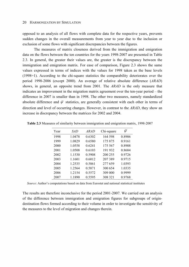
opposed to an analysis of all flows with complete data for the respective years, prevents sudden changes in the overall measurements from year to year due to the inclusion or exclusion of some flows with significant discrepancies between the figures.
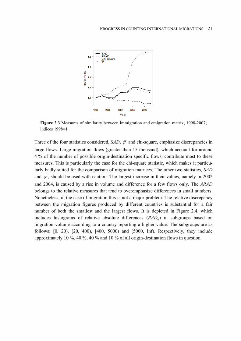
The measures of matrix closeness derived from the immigration and emigration data on the flows between the ten countries for the years 1998-2007 are presented in Table 2.3. In general, the greater their values are, the greater is the discrepancy between the immigration and emigration matrix. For ease of comparison, Figure 2.3 shows the same values expressed in terms of indices with the values for 1998 taken as the base levels (1998=1). According to the chi-square statistics the comparability deteriorates over the period 1998-2006 (except 2000). An average of relative absolute difference (ARAD) shows, in general, an opposite trend from 2001. The ARAD is the only measure that indicates an improvement in the migration matrix agreement over the ten-year period – the difference in 2007 is smaller than in 1998. The other two measures, namely standardized absolute difference and ψ statistics, are generally consistent with each other in terms of direction and level of occurring changes. However, in contrast to the ARAD, they show an increase in discrepancy between the matrices for 2002 and 2004.
Table 2.3 Measures of similarity between immigration and emigration matrix, 1998-2007
Year SAD ARAD Chi-square ψ
1998 1.0478 0.6302 164 598 0.8906 1999 1.0829 0.6580 175 875 0.9161 2000 1.0558 0.6241 175 567 0.8908 2001 1.0508 0.6103 191 932 0.8684 2002 1.1530 0.5908 200 255 0.9726 2003 1.1601 0.6012 207 389 0.9715 2004 1.2535 0.5861 277 659 1.0393 2005 1.2564 0.5871 300 654 1.0335 2006 1.2154 0.5572 309 000 0.9999 2007 1.1890 0.5595 308 321 0.9768
Source: Author’s computations based on data from Eurostat and national statistical institutes
The results are therefore inconclusive for the period 2001-2007. We carried out an analysis of the difference between immigration and emigration figures for subgroups of origin-destination flows formed according to their volume in order to investigate the sensitivity of the measures to the level of migration and changes therein.
PROGRESS IN COUNTING INTERNATIONAL MIGRATIONS
21
Figure 2.3 Measures of similarity between immigration and emigration matrix, 1998-2007; indices 1998=1
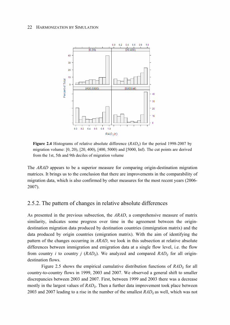
Three of the four statistics considered, SAD, ψ and chi-square, emphasize discrepancies in large flows. Large migration flows (greater than 15 thousand), which account for around 4 % of the number of possible origin-destination specific flows, contribute most to these measures. This is particularly the case for the chi-square statistic, which makes it particu-larly badly suited for the comparison of migration matrices. The other two statistics, SAD and ψ , should be used with caution. The largest increase in their values, namely in 2002 and 2004, is caused by a rise in volume and difference for a few flows only. The ARAD belongs to the relative measures that tend to overemphasize differences in small numbers. Nonetheless, in the case of migration this is not a major problem. The relative discrepancy between the migration figures produced by different countries is substantial for a fair number of both the smallest and the largest flows. It is depicted in Figure 2.4, which includes histograms of relative absolute differences (RADij) in subgroups based on migration volume according to a country reporting a higher value. The subgroups are as follows: [0, 20), [20, 400), [400, 5000) and [5000, Inf). Respectively, they include approximately 10 %, 40 %, 40 % and 10 % of all origin-destination flows in question.
HARMONIZATION BY SIMULATION
22
Figure 2.4 Histograms of relative absolute difference (RADij) for the period 1998-2007 by migration volume: [0, 20), [20, 400), [400, 5000) and [5000, Inf). The cut points are derived from the 1st, 5th and 9th deciles of migration volume
The ARAD appears to be a superior measure for comparing origin-destination migration matrices. It brings us to the conclusion that there are improvements in the comparability of migration data, which is also confirmed by other measures for the most recent years (2006-2007).
2.5.2. The pattern of changes in relative absolute differences
As presented in the previous subsection, the ARAD, a comprehensive measure of matrix similarity, indicates some progress over time in the agreement between the origin-destination migration data produced by destination countries (immigration matrix) and the data produced by origin countries (emigration matrix). With the aim of identifying the pattern of the changes occurring in ARAD, we look in this subsection at relative absolute differences between immigration and emigration data at a single flow level, i.e. the flow from country i to country j (RADij). We analyzed and compared RADij for all origin-destination flows.
Figure 2.5 shows the empirical cumulative distribution functions of RADij for all country-to-country flows in 1999, 2003 and 2007. We observed a general shift to smaller discrepancies between 2003 and 2007. First, between 1999 and 2003 there was a decrease mostly in the largest values of RADij. Then a further data improvement took place between 2003 and 2007 leading to a rise in the number of the smallest RADij as well, which was not

PROGRESS IN COUNTING INTERNATIONAL MIGRATIONS
23
the case in the previous period. Nonetheless, the number of flows with the highest differ-ences between immigration and emigration figures (RADij > 0.67) remained unchanged.
Figure 2.5 Empirical cumulative distribution functions of relative absolute difference (RADij) between immigration and emigration figures; 1999, 2003 and 2007
For ease of observation and the further analysis of transitions between specified RADij categories, relative absolute differences between immigration and emigration figures for the selected three years are also shown in histogram form in Figure 2.6. The RADij values, which were between zero and one, were divided into six categories of equal width. As noted above, the number of largest differences decreased over time and the number of smallest differences increased. As a result, we observed a U-shaped distribution of RADij in 2007. In terms of median RADij, which is less sensitive to changes in the extreme values (large or small) than the average, there was a decrease from 0.79 in 1999 to 0.65 in 2007.
Figure 2.6 Histogram of relative absolute difference (RADij) between immigration and emigration figures; 1999, 2003 and 2007

HARMONIZATION BY SIMULATION
24
In order to evaluate the dynamic aspects of the changes that occurred that were not affected by the RADij composition, we estimated for 2007 the distribution of RADij among the six defined categories using one-year transition probabilities between them calculated from data for 1999-2003. The results, together with the observed values, are presented in Figure 2.7.
Figure 2.7 Observed and estimated proportions of different categories of RADij; 2007
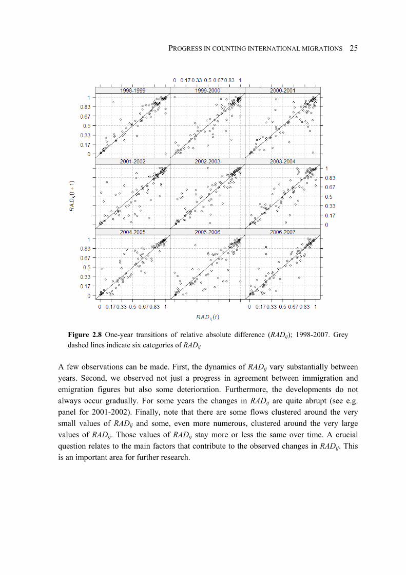
If the transition probabilities between defined categories did not change, the distribution of RADij would be less polarized. In other words, there would be fewer flows with the largest and the smallest RADij, and more with the medium ones. Thus, we do not observe a constant general improvement of agreement between origin-destination immigration and emigration figures. The development in the highest RADij has slowed down. An investiga-tion of changes in RADij over single years provides additional insights. They are presented in Figure 2.8. The points below the 45° line indicate flows for which RADij declined and the points above indicate those for which RADij increased.
PROGRESS IN COUNTING INTERNATIONAL MIGRATIONS
25
Figure 2.8 One-year transitions of relative absolute difference (RADij); 1998-2007. Grey dashed lines indicate six categories of RADij
A few observations can be made. First, the dynamics of RADij vary substantially between years. Second, we observed not just a progress in agreement between immigration and emigration figures but also some deterioration. Furthermore, the developments do not always occur gradually. For some years the changes in RADij are quite abrupt (see e.g. panel for 2001-2002). Finally, note that there are some flows clustered around the very small values of RADij and some, even more numerous, clustered around the very large values of RADij. Those values of RADij stay more or less the same over time. A crucial question relates to the main factors that contribute to the observed changes in RADij. This is an important area for further research.
HARMONIZATION BY SIMULATION
26
2.5.3. The nature of changes in relative absolute differences: remarks about future research
Any progress made in the counting of migrations that is defined in terms of agreement between figures on origin-destination flows produced by sending and receiving countries generally depends on relative changes occurring in the immigration and emigration statistics of those countries. There are two main underlying reasons for the differences between the data produced by two countries for the same flow, namely discrepancies in migration definitions and measurement errors. For ease of exposition we will not highlight coverage problems here that relate to the exclusion of selected groups of migrants from the statistics. These problems may be treated as measurement errors. Thus, changes related to definitional and measurement aspects of migration data lead to changes in data agreement. Disentangling and evaluating the impact of the two factors is, however, very problematic. An approach for tackling this issue is outlined and illustrated in this section. In addition, we use an example to show why better data agreement does not necessarily mean better data quality. Consider origin-destination migration between two countries denoted by i and j. There are two possible flows: from country i to country j (flow ij) and in the opposite direction, so from country j to country i (flow ji). Each country reports a value for each flow. Hence, for flows between a pair of countries four migration numbers come from two data collection systems: that of country i and that of country j. Two of the figures refer to immigration (IMji, IMij) and two to emigration (EMij, EMji). For clarity, information on data types is also presented in a table format (see Table 2.4).
Table 2.4 Migration statistics on flows between country i and country j
Migration statisticsa Direction of flow Country i Country j
ij (from i to j) EMij IMij ji (from j to i) IMji EMji
a IM - immigration, EM - emigration
Assume that both countries provide correct data on both immigration and emigration but apply different definitions. For instance, country i applies a three-month duration-of-stay threshold to classify movement as immigration or emigration and country j a threshold of one year. Country i, which uses a broader definition, consequently reports greater migra-tion for both the ij flow ( 0.25 1
ij ijEM IM> , where superscript denotes the applied duration of
stay criterion expressed in years) and the ji flow ( 0.25 1ji jiIM EM> ). It is, however, very
unrealistic to assume that the data are perfect and measurement errors therefore have to be considered. If the deficiencies in measuring both immigration and emigration were the
PROGRESS IN COUNTING INTERNATIONAL MIGRATIONS
27
same within and between the countries, the relationship between the figures presented above would hold. However, such assumptions are again highly questionable. First, the information on immigration and emigration available in a given country is of a different quality, because immigration is usually much better recorded than emigration. Second, measurement errors differ markedly between countries. In our example, a general superior-ity of immigration data over emigration data results, ceteris paribus, in a greater dissimilar-ity for flow ji than for flow ij ( 0.25 1 0.25 1
ji ji ij ijIM kEM kEM IM− > − , where k<1 represents a
decline in emigration data due to underestimation). Note that a significant inferiority of emigration data may lead to an emigration number reported by country i that is lower than the immigration number provided by country j ( 0.25 1
ij ijkEM IM< ), despite a broader
definition used in the former case. The difference between the two figures, however, can be relatively small. The impact of emigration underregistration may therefore be greater than that of definitional discrepancies, and the flows between the two countries (flow ij and ji) would then be reported as higher by respective destination countries. Needless to say, the slighter the difference between the duration thresholds used to qualify relocation as migration, the larger the relative impact of measurement errors on any disagreement between figures. In summary, it is useful to distinguish two types of pairs of countries (i, j): (A), those for which one country, say i, reports larger values of migration for both flow ij and flow ji, and (B), those for which higher figures are reported by destination countries, so by country j for flow ij and by country i for flow ji. For most pairs of type A, the differences between the migration figures are influenced to a substantial extent by definitional discrepancies. Due to the general worse quality of emigration data compared to immigra-tion data for flows with an emigration figure larger than immigration ( ij ijEM IM> ), the
difference is smaller than when the reverse is true ( ji jiIM EM> ). For pairs of countries
belonging to type B, it is the measurement error that plays the most important role and the differences are usually lower than for type A. Monitoring the progress in data agreement and taking into account these two types and subgroups thereof provides the possibility of at least an approximate evaluation of the character of the occurring changes, which may differ for immigration and emigration. Note that, although for ease of exposition dissimi-larity between migration figures was presented by direct comparison of their values, the resulting relationship also applies to RADij. For our analysis of relative absolute differences (RADij) between data on origin-destination specific migration among ten EU member states over a decade, it is notable that the number of pairs of countries for which receiving countries report higher values of flows than sending countries (type B) has increased considerably. In 1999 these cases constituted 11 % of all pairs of countries, whereas in 2007 their share was equal to 38 %. The sharpest increase, by 15.6 percentage points, took place in the last year. A separate investigation of RADij for these pairs of countries and for those for which one of the countries always

HARMONIZATION BY SIMULATION
28
reports a higher value (type A) leads to two important observations. First, if we only consider pairs of countries of type A, the RADij for flows with immigration figures outnumbering emigration ones are larger than the RADij for flows with emigration figures outnumbering immigration ones. It confirms as expected that the registration of immigra-tion data is better than that of emigration data. Second, flows between two countries for which the immigration data are larger regardless of direction (type B) contribute most to a rise in percentage of the small RADij. We may conclude, therefore, that the number of flows for which a measurement error is more important than differences in applied definitions is increasing. The relative differences between immigration and emigration figures for these flows are, however, relatively small. Measurement errors in the form of underregistration predominate in the emigration figures. Hence, a rise in flows for which immigration figures are larger than emigration ones may indicate a relative deterioration of emigration statistics over time. This increases the ambiguity of the development of migration statistics over time.
2.6. Conclusions
The primary goal of this chapter has been to evaluate the progress made in measuring international migration flows over a decade (1998-2007). We focused on two related questions. Has the availability of statistics on international migration flows improved over time? Furthermore, has the agreement between the emigration data produced by origin countries and the immigration data produced by destination countries become better? As regards availability, we do not observe a consistent improvement trend over time. To some extent, this is a result of the fact that some data ceased to be published due to poor quality. Reduced data availability in the most recent years is related to a delay in collecting or processing the data in some countries. This, however, means that their data lack timeliness, which is one of the dimensions of data quality. As regards comparison of data, the average of relative absolute difference (ARAD) appears to be a superior measure for comparing origin-destination migration matrices. The standardized absolute difference or the ψ statistic may be used as supplementary measures. They are, however, sensitive to changes in large flows. There has been general progress in data agreement, as indicated by ARAD. The other two measures are consistent in showing better data agreement from year to year for most years. The years 2002 and 2004 are the most apparent exceptions with a large increase in the standardized absolute difference and ψ statistic due to a rise in some large migration flows. As a result, these measures show that the data similarity in 2007 was worse than in 1998. The changes in RADij may be summarized as a decrease in the percentage of the largest values and an increase in the percentage of the smallest values. Nevertheless, there is no consistent pattern of improvement in data agreement over time. In

PROGRESS IN COUNTING INTERNATIONAL MIGRATIONS
29
addition, an increase in the share of small RADij is connected with a rise in the number of flows for which the destination country reports a higher value of migration than the origin country. This may be a sign that measurement-related problems rather than definitional ones are having an increased impact. If definitions alone played a role, a country that applies a broader definition of migration would report larger flows for both directions. It is difficult, however, to disentangle the actual impact of definition discrepancies from the impact of measurement errors. Valuable insights may be obtained from a microsimulation approach. A series of different definitions of migration might be applied to individual relocation histories simulated under different assumptions. The migration flow statistics derived for the whole virtual population would reveal the impact of the applied migration definitions on the resulting migration figures. In conclusion, progress in counting migrations was much slower than could have been expected over a decade. Comprehensive measures indicating some improvements in agreement between the emigration data produced by origin countries and the immigration data produced by destination countries are not free from ambiguities, in particular when analyzed at a disaggregated level. Further research is therefore needed to investigate the main factors contributing to differences between migration statistics. More importantly, some effective measures still have to be taken to improve the quality of statistics on international migration. Cooperation between countries, as successfully implemented in Nordic countries, may serve as a role model. In addition, however, a harmonized definition of migration should be employed by all countries.
References
Butterfield M, Mules T. 1980. A testing routine for evaluating cell by cell accuracy in short-cut regional input-output tables. Journal of Regional Science 20:293-310.
European Commission. 2007. Regulation (EC) No 862/2007 of the European Parliament and of the Council of 11 July 2007 on Community statistics on migration and international protection. European Commission: Brussels. Available at: http://eur-lex.europa.eu/LexUriServ/LexUri Serv.do?uri=OJ:L:2007:199:0023:0029:EN:PDF [accessed 10 April 2010].
Fotheringham AS, Knudsen DC. 1987. Goodness-of-Fit Statistics. Geo Books: Norwich.
Herm A. 2008. Recommendations on international migration statistics and development of data collection at an international level. In International Migration in Europe: Data, Models and Estimates, Raymer J, Willekens F (eds.); John Wiley & Sons, Ltd: Chichester; 41-71.
Kelly JJ. 1987. Improving the comparability of international migration statistics: contributions by the Conference of European Statisticians from 1971 to date. International Migration Review 21:1017-1037.

HARMONIZATION BY SIMULATION
30
Knudsen DC, Fotheringham AS. 1986. Matrix comparison, goodness-of-fit, and spatial interaction modeling. International Regional Science Review 10:127-147.
Kupiszewska D, Nowok B. 2008. Comparability of statistics on international migration flows in the European Union. In International Migration in Europe: Data, Models and Estimates, Raymer J, Willekens F (eds.); John Wiley & Sons, Ltd: Chichester; 41-71.
Poulain M. 1999. International migration within Europe: towards more complete and reliable data? Paper presented at Joint ECE-Eurostat Work Session on Demographic Projections, Pe-rugia, May 1999.
Poulain M, Perrin N, Singleton A (eds.). 2006. THESIM: Towards Harmonised European Statistics on International Migration. Presses Universitaires de Louvain: Louvain-la-Neuve.
R Development Core Team. 2009. R: A language and environment for statistical computing. Vienna, Austria: R Foundation for Statistical Computing. Available at http://www.R-project. org.
United Nations. 1998. Recommendations on Statistics of International Migration: Revision 1. Statistical Papers, No. 58, Rev.1 Sales No. E.98.XVII.14: New York.
Voas D, Williamson P. 2001. Evaluating goodness-of-fit measures for synthetic microdata. Geographical & Environmental Modelling 5:177-200.
Willekens F, Por A, Raquillet R. 1979. Entropy, multiproportional, and quadratic techniques for inferring detailed migration patterns from aggregate data. Mathematical theories, algorithms, applications, and computer programs. IIASA Working Paper WP-79-088, The International Institute for Applied Systems Analysis: Laxenburg, Austria.
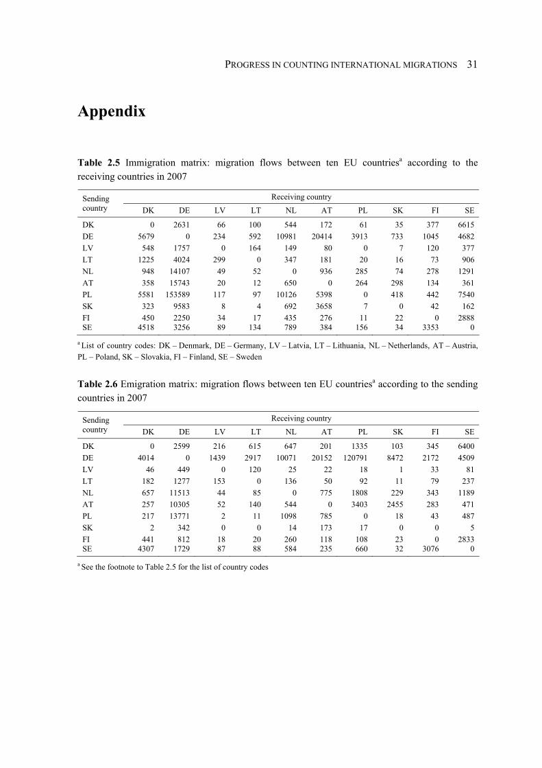
PROGRESS IN COUNTING INTERNATIONAL MIGRATIONS
31
Appendix
Table 2.5 Immigration matrix: migration flows between ten EU countriesa according to the receiving countries in 2007
Receiving country Sending country DK DE LV LT NL AT PL SK FI SE
DK 0 2631 66 100 544 172 61 35 377 6615 DE 5679 0 234 592 10981 20414 3913 733 1045 4682 LV 548 1757 0 164 149 80 0 7 120 377 LT 1225 4024 299 0 347 181 20 16 73 906 NL 948 14107 49 52 0 936 285 74 278 1291 AT 358 15743 20 12 650 0 264 298 134 361 PL 5581 153589 117 97 10126 5398 0 418 442 7540 SK 323 9583 8 4 692 3658 7 0 42 162 FI 450 2250 34 17 435 276 11 22 0 2888 SE 4518 3256 89 134 789 384 156 34 3353 0
a List of country codes: DK – Denmark, DE – Germany, LV – Latvia, LT – Lithuania, NL – Netherlands, AT – Austria, PL – Poland, SK – Slovakia, FI – Finland, SE – Sweden
Table 2.6 Emigration matrix: migration flows between ten EU countriesa according to the sending countries in 2007
Receiving country Sending country DK DE LV LT NL AT PL SK FI SE
DK 0 2599 216 615 647 201 1335 103 345 6400 DE 4014 0 1439 2917 10071 20152 120791 8472 2172 4509 LV 46 449 0 120 25 22 18 1 33 81 LT 182 1277 153 0 136 50 92 11 79 237 NL 657 11513 44 85 0 775 1808 229 343 1189 AT 257 10305 52 140 544 0 3403 2455 283 471 PL 217 13771 2 11 1098 785 0 18 43 487 SK 2 342 0 0 14 173 17 0 0 5 FI 441 812 18 20 260 118 108 23 0 2833 SE 4307 1729 87 88 584 235 660 32 3076 0
a See the footnote to Table 2.5 for the list of country codes


33
3. A probabilistic framework for harmonization of migration statistics
Abstract. Inadequate and inconsistent data are a common and persistent problem in the field of migration. Deficiencies in migration statistics may be tackled using modelling techniques, something that has recently been recognized by European Union (EU) policymakers. The new Regulation on Community statistics on migration and international protection, which obliges countries to supply harmonized statistics, provides the possibility of using estimation methods to adapt statistics based on national definitions to comply with the required one-year duration of stay definition. The main objective of this chapter is to provide a theoretical probabilistic framework for capturing the various migration flow statistics that are available. It is a crucial step towards gaining a better understanding of the data and consequently harmonizing it. Different migration measures represent the same continuous data-generating process. They differ according to how the data happened to be collected and how the statistics happened to be produced. We introduce the key concepts of migration statistics using a simple duration model, namely an exponential distribution. While more complex models can better reflect the reality, they do not fundamentally modify the framework presented. The main focus is placed on the time criterion used in migration definition. This refers to duration of stay following relocation, which different countries specify very differently and which constitutes the main source of discrepancies in the operationalization of a migration concept in the EU member states.
A probabilistic framework for harmonisation of migration statistics, Nowok B, Willekens F, Population, Space and Place DOI: 10.1002/psp.624. Copyright © 2010 John Wiley & Sons, Ltd.

HARMONIZATION BY SIMULATION
34
3.1. Introduction
Data on international migration are lacking in terms of quality and cross-country compara-bility, which severely constrains analysis of migration patterns and their demographic, economic and social implications. The international migration debate in Europe and the European migration policy that is being implemented require, without doubt, high quality migration statistics that can be compared internationally. In August 2007, the new Regula-tion of the European Parliament and of the Council on Community statistics on migration and international protection entered into force (European Commission, 2007). The Regulation establishes a legal basis for the collection and compilation of migration statistics. It focuses on the comparability of statistical outputs and obliges member states, starting from the reference year 2009, to provide migration statistics that comply with a harmonized definition. The Regulation provides for the possibility of using statistical estimation methods to adapt statistics based on national definitions so that they comply with the harmonized definition. This emphasizes the importance of investigating such methods. The purpose of this chapter is to present a probabilistic framework that is able to accommodate different definitions of migration and that may be used to convert different types of migration data into migration statistics with a harmonized definition. We intend to show that migration modelling is an effective approach to the harmonization of migration statistics. Currently, there is a considerable variability in the migration definitions applied by the countries of Europe. It results from the complexity of the migration process and the different national practices for measuring it. The key problem with defining migration stems from the fact that individual movements are situated in a time continuum. Spatial population movements include travel, commuting and migration. Migration is generally defined as a change of residence (address). However, the vagueness of residence and the coexistence of different types of residence (e.g. actual, usual and legal residence; tempo-rary and permanent residence) lead to different conceptualizations of migration itself. An individual’s place of residence is usually determined by a duration-of-stay criterion, e.g. three months, one year or ‘permanent’. As a result, migration is a change of place of residence for at least three months, one year or ‘for good’ respectively (for details on migration flow statistics in the EU-25 see Kupiszewska and Nowok, 2008; Nowok et al., 2006). The duration of stay may be intended or actual. The intended duration of stay is based on a person’s intentions and these are usually revised over time as circumstances change. Consequently, it is possible that they differ from the actual length of stay. A final operational definition of migration is very often a compromise between the concept of migration and available data sources. This increases the variability of possible measures. Courgeau (1973) introduced a crucial distinction between migrations and migrants. Essentially, migration count should refer to the number of moves and migrant count to the number of persons who move at least once during a reference period. Nonethe-

A PROBABILISTIC FRAMEWORK FOR HARMONIZATION
35
less, the number of migrants is often approximated through a typical census question about a place of residence at a previous date. Moreover, the migration definition may vary across subpopulations such as nationals and foreigners, for example. It may also be different for immigration and emigration, and it may change over time. There are numerous studies that discuss conceptual and measurement issues relating to migration, e.g. Bell et al. (2002), Bilsborrow et al. (1997), Poulain (1999; 2001), Poulain et al. (2006), United Nations (2002), Willekens (1982; 1985) and Zlotnik (1987). The need to analyze migration patterns across time and countries has motivated the development of modelling techniques for overcoming the deficiencies present in migration statistics. Such attempts are, however, limited. Courgeau (1973) developed a model that relates the number of migrations to the census-based number of migrants. His method deals with multiple and return migrations. The hazard rates of migration are assumed to be constant and only part of the population can migrate again. Note that Courgeau’s model (1973) does not tackle the problems of migration definition itself. It was used mainly to study temporal trends in internal migration in France using census data for various geographical subdivisions (e.g. Baccaïni, 2007; Courgeau and Lelièvre, 2004). The model specification does not depend on spatial units that are analyzed, but the resulting parameter estimates are usually affected. The latter feature of the model also applies to the framework presented in this chapter. A recently completed Eurostat project entitled MIMOSA – Migration Modelling for Statistical Analyses (http://mimosa.gedap.be/) – worked out a method for harmonizing international migration data available in Europe (De Beer et al., 2009). The authors use origin-destination specific flows as reported by sending and receiving countries to estimate a set of adjustment factors for both immigration and emigration figures that minimize the differences between the two available datasets. The correction factors are obtained using a constrained optimization procedure. In principle, this is the same approach to the harmoni-zation of international migration data as that suggested by Poulain (1993) and later revised by Poulain and Dal (2008). A recent study by Abel (2009) provides a useful overview of the method and explores various alternative distance measures and constraint functions. Note that these methods do not provide answers about the linkage of one measure of migration to another. The values of the correction factors indicate the level of discrepan-cies between figures reported by different countries, but the definitional problems alone are not the cause of these differences. This chapter focuses directly on migration definition. It approaches the migration process from a probabilistic perspective and views migration as a random event, i.e. an outcome of an underlying random process. By modelling the migration process, events and more particularly the distribution of events can be predicted. In studies of migration, a probabilistic approach is very natural and has been used for several decades (see e.g. Allison, 1985; Bijwaard, 2008; Constant and Zimmermann, 2003; 2007; Davies et al., 1982; Ginsberg, 1971; 1972; 1979a; 1979b; Pickles, 1983). The novelty of this study is

HARMONIZATION BY SIMULATION
36
that it applies probability theory to the harmonization of migration statistics. To tackle the issue properly, a distinction must be made between the migration process and the meas-urement process. Measuring is determining the magnitude or the characteristics of something. All measurements involve error but ideally errors remain within predefined limits. Unless the true process is known, measurement errors cannot be quantified. Hence, a few crucial questions have to be addressed before harmonization can be tackled. First, what is the true migration process? Second, how is migration measured? Third, what is the impact of the use of various measurements on the recorded level of migration flows? Finally, how can we obtain harmonized migration statistics from the available data? All these issues will be addressed in turn. The chapter consists of five sections. Section 3.2 briefly presents the probabilistic model of migration, which is well documented in the literature. The basic parameter of the model is the instantaneous rate of relocation. This rate is referred to as relocation intensity or hazard rate of relocation. Section 3.3 reviews different measures of migration that are commonly used to produce migration statistics. In Section 3.4, the different migration measures are related to the basic parameters of the migration model. In other words, measures that result from different types of observation of migration are linked to the instantaneous rates of relocation, providing a powerful instrument for the harmonization of migration statistics. Section 3.5 concludes the chapter.
3.2. Migration process
There are two general approaches to modelling migration. The first is to model the data. A model is chosen that fits the data best, given a criterion of goodness of fit. In the second approach, an attempt is made to look behind the data and focus on the process itself. Model specification is of paramount importance here and the data are used to obtain the parame-ters of the model that is believed to describe the process accurately. The latter strategy, even though it may sometimes be speculative, should be given priority in the fields where very different measurements of the process are used. Migration is an obvious example of such a process. Thus, a migration process rather than migration data should be a point of departure.
We begin by assuming that migration is an unambiguously defined event that oc-curs at a specific point in time. Hereinafter this event is referred to as relocation, as distinct from operational definitions of the migration event that are used to produce migration statistics. In general terms, relocation is a change of residence (address). It may occur repeatedly for individuals at any point in time. A complete relocation history of an individual within a specific observation period is denoted here by ω. It may be presented in a compact way:
A PROBABILISTIC FRAMEWORK FOR HARMONIZATION
37
[ ] { }0 0 0 1 1e n n e et ,t t , y ,t , y , ,t , y , ,t , yω = … … , (3.1)
where 0t is the onset of observation (beginning of the observed residence history) and 0y
the place of residence at that time, nt is the date of the n-th relocation and ny is the place
of residence following the n-th relocation, et denotes the end of observation and ey the
place of residence at that time (Tuma and Hannan, 1984; Willekens, 1999). From this information we can infer where a person is living at every moment in the observation period. From the perspective of stochastic processes expression (3.1) is a realization (sample path) of the underlying process. This relocation process may be described using counts (numbers of events in a given period of time) or waiting times (periods of time between successive events) (for a review of methods of analysis for repeated events see e.g. Cook and Lawless, 2002). In the context of migration statistics, aspects of both counts and waiting times are of particular relevance. We are interested in the total number of migrations, which are usually relocations with some conditions imposed on waiting times. Measures of migrations are discussed in detail in Section 3.3. The theory of counting processes (also referred to as arrival processes or point processes) therefore provides a useful general framework for the study of migration (Andersen et al., 1993). The counting process enables one to study the number and timing of events. It provides the possibility of making a straightforward connection between models for counts and duration models. Below we briefly describe a counting process and then the above-mentioned connection. A counting process ( ){ }0N t t ≥ is a stochastic process which counts the number
of events as they occur up to and including time t. The process has the properties that ( )0 0N = , ( )N t < ∞ with a probability of one and the sample paths of ( )N t are right-
continuous and piecewise constant with jumps of size +1. The counting process is fully described by its random intensity process λ(t) (for details on the concept of intensity see e.g. Blossfeld et al., 1989; Blossfeld and Rohwer, 2002; Klein and Moeschberger, 2003). For a short time interval [ ),t t dt+ , ( )t dtλ is the conditional probability of an event
(relocation) in that interval, given all that has happened until just before t (Aalen et al., 2008, pp. 26-27). Note that modelling recurrent events through their intensity functions is a very general and convenient approach. Let nT denote the arrival time of the n-th event. It is
easy to observe that the time of n-th event is before or at t if and only if the number of arrivals in [ ]0, t is equal to n or more. This reasoning gives the following relationship
between waiting times and the number of events
( )nT t N t n≤ ⇔ ≥ . (3.2)
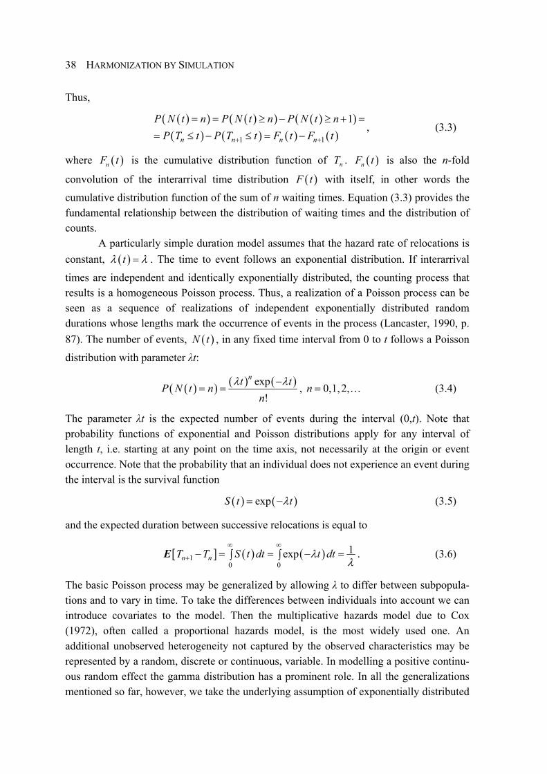
HARMONIZATION BY SIMULATION
38
Thus,
( )( ) ( )( ) ( )( )
( ) ( ) ( ) ( )1 1
1
n n n n
P N t n P N t n P N t nP T t P T t F t F t+ +
= = ≥ − ≥ + =
= ≤ − ≤ = −, (3.3)
where ( )nF t is the cumulative distribution function of nT . ( )nF t is also the n-fold
convolution of the interarrival time distribution ( )F t with itself, in other words the
cumulative distribution function of the sum of n waiting times. Equation (3.3) provides the fundamental relationship between the distribution of waiting times and the distribution of counts. A particularly simple duration model assumes that the hazard rate of relocations is constant, ( )tλ λ= . The time to event follows an exponential distribution. If interarrival
times are independent and identically exponentially distributed, the counting process that results is a homogeneous Poisson process. Thus, a realization of a Poisson process can be seen as a sequence of realizations of independent exponentially distributed random durations whose lengths mark the occurrence of events in the process (Lancaster, 1990, p. 87). The number of events, ( )N t , in any fixed time interval from 0 to t follows a Poisson
distribution with parameter λt:
( )( ) ( ) ( )exp!
nt tP N t nn
λ λ−= = , 0,1,2,n = … (3.4)
The parameter λt is the expected number of events during the interval (0,t). Note that probability functions of exponential and Poisson distributions apply for any interval of length t, i.e. starting at any point on the time axis, not necessarily at the origin or event occurrence. Note that the probability that an individual does not experience an event during the interval is the survival function
( ) ( )expS t tλ= − (3.5)
and the expected duration between successive relocations is equal to
[ ] ( ) ( )10 0
1expn nT T S t dt t dtλλ
∞ ∞
+ − = = − =∫ ∫E . (3.6)
The basic Poisson process may be generalized by allowing λ to differ between subpopula-tions and to vary in time. To take the differences between individuals into account we can introduce covariates to the model. Then the multiplicative hazards model due to Cox (1972), often called a proportional hazards model, is the most widely used one. An additional unobserved heterogeneity not captured by the observed characteristics may be represented by a random, discrete or continuous, variable. In modelling a positive continu-ous random effect the gamma distribution has a prominent role. In all the generalizations mentioned so far, however, we take the underlying assumption of exponentially distributed

A PROBABILISTIC FRAMEWORK FOR HARMONIZATION
39
interarrival times and the Poisson distribution for counts. A count data model with substantially higher flexibility than the Poisson model is obtained if we allow the intensity to vary not only between individuals but also with duration of stay. Distributions that capture duration dependence of the event occurrence include, inter alia, Weibull, Gompertz, gamma and lognormal distribution. Both Weibull and gamma distribution are generalizations of the exponential distribution and the resulting count data models nest the Poisson model. The specification of the count model that is consistent with an assumed waiting time distribution other than the exponential one is, however, not straightforward (see McShane et al., 2008 for Weibull distribution; and Winkelmann, 1995 for gamma distribution). In this study we use a Poisson process. This does not affect the basic idea of the framework presented. An extension of the model is necessary in order to capture better the complexities of either human behaviour or data collection systems that may function differently for nationals and foreigners, and for immigration and emigration.
3.3. Observation plans and measures
The relocation process is a continuous and recurrent phenomenon. To collect data gener-ated by such a process, different observation plans, i.e. different schemes for collecting systematic information, can be used (Blossfeld and Rohwer, 2002; Tuma and Hannan, 1984). If we do not consider direction of relocation, the exact timings of all relocations experienced by each individual under study is the most complete information that can be available (compare with expression (3.1)). In practice, however, the collection of such relocation data is usually not feasible. For operational reasons, the migration event is defined in such a way that it can be practically measured. As a result, relocation processes are observed and measured in very different manners. It is of great importance, therefore, to understand the actual meaning of migration statistics in order to make a correct link with the underlying process. This section proposes a useful typology of existing migration data. The main data types are summarized in Table 3.1. Recall first that the relocation history of an individual can be viewed from two different perspectives. In the first, the relocation history is described in terms of the events and their timing (event approach). In the second, the relocation history is described in terms of the places of residence at consecutive points in time (status approach). The intervals between the reference points can be of different lengths. Rajulton (2001) provides a direct connection between the event and status approaches by defining an event as a transition between statuses (states). Consider now a well-established distinction between migration data and migrant data. Essentially, migration denotes the act of moving (event) and migrant denotes the person performing the act (Courgeau, 1974). For a given reference period, a migrant is a person who moves at least once during this time interval. The

HARMONIZATION BY SIMULATION
40
number of migrants is often estimated using a census or survey question about the place of residence at a previous date and is thus based on status data. As indicated by Courgeau (1973), this estimation is not satisfactory because return and non-surviving migrants are not enumerated. Nonetheless, in the migration literature the distinction described above between event data and status data (e.g. Ledent, 1980; Willekens, 1999) is usually treated as equivalent to the distinction between migration data and migrant data. Thus, in such an approach migrant denotes a person who moves at least once during a reference period and who lives in a different place at the end of the period than at the beginning. The event data and status data are also called movement data and transition data respectively (Rees and Willekens, 1986). As events are sometimes defined as transitions between statuses, for the sake of precision transition data can be called discrete transition data as opposed to direct transition data referring to movement data. In this study we distinguish three separate categories: migration data, migrant data (as defined by Courgeau, 1973) and discrete transition data (hereinafter referred to as transition data).
Table 3.1 Main types of migration data
Type Description Alternative names in the literature
(Conditional) migration Event Movement, direct transition (Conditional) migrant Person experiencing an event at least
once during a reference period -
Transition Status of having a different place of residence at a specified date in the past
Migrant, discrete transition
We now introduce more specific data types that are particularly relevant for the harmonization of migration statistics. In official statistics the migration concept often involves a minimum duration of stay (actual or intended) to distinguish migration from other movements. Thus, migration is defined as a change in residence that is followed by a minimum duration of stay. The measurement of migration and migrants, which is condi-tional on a minimum duration of stay, leads to two data types that we call conditional migration data and conditional migrant data. The conditional migration data refer to migrations that are followed by a stay of specified duration, i.e. a person does not leave his or her new place of residence during that period. The conditional migrant data refer to migrants who experience at least one migration followed by a stay of a specified duration. As mentioned in the introduction, the duration may be intended or actual, where the former can be either shorter or longer than the latter. In this study we focus on actual duration assuming that all intentions are realized. The rationale behind the focus on conditional data types is the widespread use of an approach of this kind, especially in Europe. Note that data following a definition of a long-term migrant recommended by the United Nations (United Nations, 1998) falls into the category of conditional migrant data. This covers people who change their country of usual residence for a period of at least a year.
A PROBABILISTIC FRAMEWORK FOR HARMONIZATION
41
3.4. Indicators of migration process
As shown in the previous section, we received different results for the same underlying data-generating process depending on how the data happened to be collected and how the statistics happened to be produced. In this section we link empirical migration measures with an underlying relocation process. The connection is made through relocation intensity λ(t), which governs the process. For ease of exposition, we assume that members of a population migrate independently and that their migration experience may be described by the same Poisson process with the constant intensity λ. The model was presented in Section 3.2. We start with the movement approach and consider the conditional migration and conditional migrant measures, and relationships between the two. Then, we present transition data and compare them with data produced using a movement approach.
Counting all relocations, without any restriction on the duration of stay in a destina-tion place, leads to the expected number of λt relocations in a time period of length t (hereinafter t without a subscript denotes the length of reference period). In practice, however, only selected relocations are counted as migrations. The concept of conditional migration, as described in Section 3.3, distinguishes migration from all relocations based on the minimum length of continuous stay that must follow change of place of residence. Thus, a person experiences a conditional migration when he or she changes place of residence and then does not do it again within a time interval of a fixed length of mt . In
other words, a person ‘survives’ time mt without any movement. Note that the requirement
of continuity of stay is a simplifying assumption. In practice, some interruptions may occur, especially when a duration threshold of mt is relatively long. If the relocation rate is
constant, the probability of being a stayer after mt is a survivor function of an exponential
distribution or zero term in a Poisson distribution. Therefore, an expected number of conditional migrations with a duration threshold equal to mt experienced by an individual
over a period of length t is derived from the Poisson distribution with a parameter cor-rected for survival of at least mt
( ) ( )( ) ( )( ) ( )0
exp exp exp exp!m
nm m
t mn
t t t tN t n t tn
λ λ λ λ λ λ∞
=
− − −⎡ ⎤ = = −∑⎣ ⎦E (3.7)
The survivor function ( )exp mtλ− may be interpreted as the proportion of migrations that
satisfy the duration-of-stay criterion. Thanks to a stochastic approach we know the chances of staying for various durations of mt , even if the actual realizations take place beyond the
reference period t. In the special case when 0mt = all relocations are counted. From (3.7)
we discover an important relationship between counts of conditional migrations for two different durations of stay,
1mt and 2mt :
HARMONIZATION BY SIMULATION
42
( )
( )( )( )1
1 2
2
expm
m
tm m
t
N tt t
N tλ
⎡ ⎤⎣ ⎦ = − −⎡ ⎤⎣ ⎦
E
E. (3.8)
The relationship depends on the relocation intensity but is independent of the length of the reference period t. Below we present discrepancies between migration figures with different duration-of-stay criteria under various assumptions about relocation intensity. Since a one-year duration is recommended by the United Nations and required by the EU Regulation (European Commission, 2007; United Nations, 1998), we use it as a reference level. Thus, the values of the ratio (3.8) were calculated for different durations applied in the migration definition, [ ]
10;5m mt t= ∈ , relative to the UN definition,
21mt = , and selected
relocation intensity, ( ]0;1λ ∈ . The choice of the considered values of mt is determined by
the lengths of duration criteria that are used in practice. Most often the duration threshold is equal to three months, six months or one year (Kupiszewska and Nowok, 2008). A threshold equal to zero refers to a migration definition with no duration criterion. Migra-tion for at least five years may be seen as an approximation of a ‘permanent’ migration (Nowok, 2008). As regards the considered relocation intensities, the high values may be justified in the framework of a mover-stayer model. Only part of a population consists of potential migrants and the relocation intensity should therefore refer to these people. The results are presented in the left panel of Figure 3.1. For instance, if the migration intensity equals 0.2 (dotted line) and we count migrations for half a year,
10.5mt = , instead of one
year, we report figures that are higher by around 10 %. For the same migration rate of 0.2, counting migrations for five years,
15mt = , results in an underestimation of the measure of
migration by approximately 55 %. For the low levels of relocation intensities discrepancies between counts of migrations for different durations are relatively small. An increase in differences with a higher relocation rate results from the fact that with the increasing intensity a person relocates more often. In other words, durations between subsequent relocations become shorter and shorter and we observe multiple migrations for a short duration for the same individual and at the same time only a limited number of migrations for a longer duration. To get some idea of the discrepancies in actual migration data with different duration of stay criterion, compare figures on migration from Poland to Sweden in 1998-2007 produced by the two countries. This is equivalent to a comparison between the ‘permanent’ and one-year criterion used in Polish and Swedish data respectively. Depending on year, Poland reported numbers lower by 65-94 %. The disagreements may, however, also result from sources other than definitional ones, such as measurement errors.
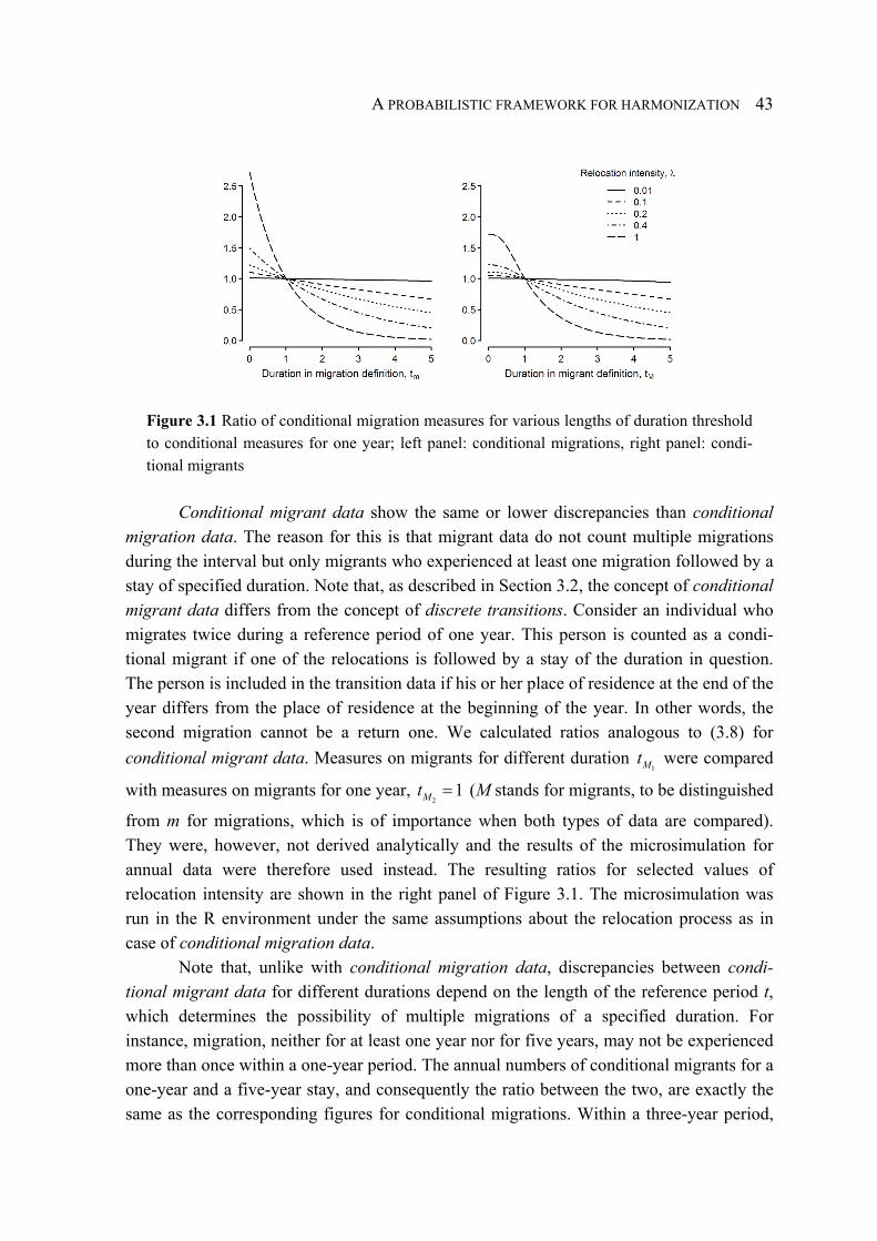
A PROBABILISTIC FRAMEWORK FOR HARMONIZATION
43
Figure 3.1 Ratio of conditional migration measures for various lengths of duration threshold to conditional measures for one year; left panel: conditional migrations, right panel: condi-tional migrants
Conditional migrant data show the same or lower discrepancies than conditional migration data. The reason for this is that migrant data do not count multiple migrations during the interval but only migrants who experienced at least one migration followed by a stay of specified duration. Note that, as described in Section 3.2, the concept of conditional migrant data differs from the concept of discrete transitions. Consider an individual who migrates twice during a reference period of one year. This person is counted as a condi-tional migrant if one of the relocations is followed by a stay of the duration in question. The person is included in the transition data if his or her place of residence at the end of the year differs from the place of residence at the beginning of the year. In other words, the second migration cannot be a return one. We calculated ratios analogous to (3.8) for conditional migrant data. Measures on migrants for different duration
1Mt were compared
with measures on migrants for one year, 2
1Mt = (M stands for migrants, to be distinguished
from m for migrations, which is of importance when both types of data are compared). They were, however, not derived analytically and the results of the microsimulation for annual data were therefore used instead. The resulting ratios for selected values of relocation intensity are shown in the right panel of Figure 3.1. The microsimulation was run in the R environment under the same assumptions about the relocation process as in case of conditional migration data.
Note that, unlike with conditional migration data, discrepancies between condi-tional migrant data for different durations depend on the length of the reference period t, which determines the possibility of multiple migrations of a specified duration. For instance, migration, neither for at least one year nor for five years, may not be experienced more than once within a one-year period. The annual numbers of conditional migrants for a one-year and a five-year stay, and consequently the ratio between the two, are exactly the same as the corresponding figures for conditional migrations. Within a three-year period,

HARMONIZATION BY SIMULATION
44
multiple migrations are possible in the case of migration for one year but not for five years. As a result, the multiple migrations that are not included in statistics on migrants diminish the discrepancy between one-year and five-year conditional migrant data compared to conditional migration data. We focused our attention, however, on annual data because annual statistics are most common in practice. In fact, the impact of counting migrants instead of migrations on discrepancies between annual measures for different durations is of importance for a time criterion shorter than half a year. For longer durations the number of multiple migrants is negligible (see Figure 3.2).
Figure 3.2 Conditional migrations per conditional migrant for the same duration tm = tM; annual data
In principle, knowledge of the relocation rate enables us to recalculate counts of migrations or migrants for a specific duration (conditional migrations and conditional migrants respectively) into migrations or migrants for any other required duration. An example of the relationship between these types of annual measures for durations of up to one year and intensity 0.2λ = is presented in Figure 3.3. The solid line represents a contour line of the value of one. For the corresponding pairs of duration thresholds mt and
Mt used in migration and migrant definitions respectively, the annual number of condi-
tional migrations is equal to the annual number of conditional migrants. For instance, besides the obvious case of migrations and migrants for one year, the number of migrants for two months is approximately equal to the number of migrations for half a year. In other cases, if the data at our disposal refer to migrants for a specific duration and we would like to know the number of migrations for the same or different duration, we have to multiply our figure by the value indicated by the grey scale. For a relocation rate equal to 0.2, the discrepancy between the narrowest and the broadest measure within a one-year duration limit, namely the number of conditional migrants for one year, 1Mt = , and the number of
all (non-conditional) migrations, 0mt = , respectively, equals 22 % (upper left corner of

A PROBABILISTIC FRAMEWORK FOR HARMONIZATION
45
Figure 3.3). This means that, during a period of one year, the number of migrations without any duration-of-stay restriction is 22 % greater than the number of migrants under the one-year duration of stay criterion. If we raise the hazard rate from 0.2 to 0.4, the difference increases to 50 %. Thus, for conditional measures of a duration of up to one year, which are usually used in practice, we should not expect differences greater than 50 %. Nonethe-less, if the widest measure is the conditional migrants for five years, which may approxi-mate the measure of permanent migrants applied, for example, by some former state socialist countries, the difference increases to 172 % for intensity 0.2λ = . For a migration rate equal to 0.4 the number of migrants for five years amount to less than 14 % of the number of migrations without any duration of stay restriction. This percentage decreases rapidly with the increasing intensity, for instance, it amounts to 2 % for 0.8λ = , but such a high international migration rate is vastly unrealistic.
Figure 3.3 Ratio of conditional migrations to conditional migrants, for various durations up to one year and intensity λ=0.2; solid line is a contour line of value one; dashed line is a line of equality of tm and tM
It is noteworthy that due to the distinction between migration and migrant measures, data with a longer duration-of-stay condition may be larger than data with a shorter one. In Figure 3.3, the area between the solid line (a contour line with a value of one) and the dashed line (a line of equality of duration condition in migration and migrant definition) includes combinations of lengths of duration threshold used in migration and migrant definition for which conditional migration numbers are greater than conditional migrant numbers, despite a longer duration criterion being used in the former case. For example, data on migrations for three months are larger by about 5 % than data on migrants for one month. The number of combinations of duration thresholds for which the aforementioned relationship holds increases slightly with declining relocation intensity. At the same time, the lower the hazard rate of relocation, the lower the differences between the considered
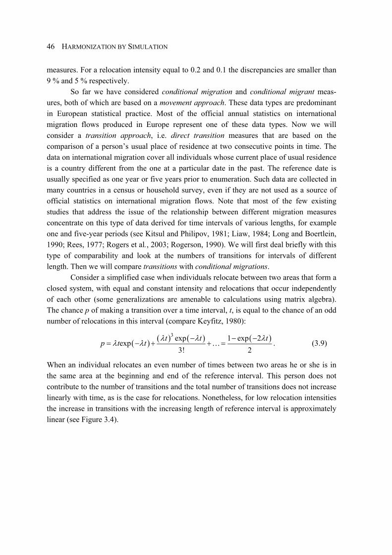
HARMONIZATION BY SIMULATION
46
measures. For a relocation intensity equal to 0.2 and 0.1 the discrepancies are smaller than 9 % and 5 % respectively.
So far we have considered conditional migration and conditional migrant meas-ures, both of which are based on a movement approach. These data types are predominant in European statistical practice. Most of the official annual statistics on international migration flows produced in Europe represent one of these data types. Now we will consider a transition approach, i.e. direct transition measures that are based on the comparison of a person’s usual place of residence at two consecutive points in time. The data on international migration cover all individuals whose current place of usual residence is a country different from the one at a particular date in the past. The reference date is usually specified as one year or five years prior to enumeration. Such data are collected in many countries in a census or household survey, even if they are not used as a source of official statistics on international migration flows. Note that most of the few existing studies that address the issue of the relationship between different migration measures concentrate on this type of data derived for time intervals of various lengths, for example one and five-year periods (see Kitsul and Philipov, 1981; Liaw, 1984; Long and Boertlein, 1990; Rees, 1977; Rogers et al., 2003; Rogerson, 1990). We will first deal briefly with this type of comparability and look at the numbers of transitions for intervals of different length. Then we will compare transitions with conditional migrations.
Consider a simplified case when individuals relocate between two areas that form a closed system, with equal and constant intensity and relocations that occur independently of each other (some generalizations are amenable to calculations using matrix algebra). The chance p of making a transition over a time interval, t, is equal to the chance of an odd number of relocations in this interval (compare Keyfitz, 1980):
( ) ( ) ( ) ( )3 exp 1 exp 2exp3! 2
t t tp t t λ λ λλ λ − − −= − + + =… . (3.9)
When an individual relocates an even number of times between two areas he or she is in the same area at the beginning and end of the reference interval. This person does not contribute to the number of transitions and the total number of transitions does not increase linearly with time, as is the case for relocations. Nonetheless, for low relocation intensities the increase in transitions with the increasing length of reference interval is approximately linear (see Figure 3.4).
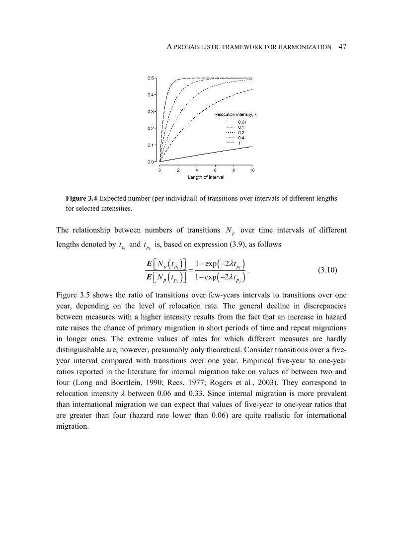
A PROBABILISTIC FRAMEWORK FOR HARMONIZATION
47
Figure 3.4 Expected number (per individual) of transitions over intervals of different lengths for selected intensities.
The relationship between numbers of transitions pN over time intervals of different
lengths denoted by 1pt and
2pt is, based on expression (3.9), as follows
( )( )
( )( )
1 1
2 2
1 exp 2
1 exp 2p p p
p p p
N t t
N t t
λ
λ
⎡ ⎤ − −⎣ ⎦ =⎡ ⎤ − −⎣ ⎦
E
E. (3.10)
Figure 3.5 shows the ratio of transitions over few-years intervals to transitions over one year, depending on the level of relocation rate. The general decline in discrepancies between measures with a higher intensity results from the fact that an increase in hazard rate raises the chance of primary migration in short periods of time and repeat migrations in longer ones. The extreme values of rates for which different measures are hardly distinguishable are, however, presumably only theoretical. Consider transitions over a five-year interval compared with transitions over one year. Empirical five-year to one-year ratios reported in the literature for internal migration take on values of between two and four (Long and Boertlein, 1990; Rees, 1977; Rogers et al., 2003). They correspond to relocation intensity λ between 0.06 and 0.33. Since internal migration is more prevalent than international migration we can expect that values of five-year to one-year ratios that are greater than four (hazard rate lower than 0.06) are quite realistic for international migration.

HARMONIZATION BY SIMULATION
48
Figure 3.5 Ratio of transitions over an interval of different lengths to transitions over one year.
Under the simplifying assumptions stated above we can derive a relationship be-tween transitions over intervals of a different length and conditional migrations for various durations of stay. We considered only the case when transitions and migrations are observed in intervals of the same length of t, i.e. when the reference period for conditional migrations number is equal to the interval over which we count the number of transitions. The length of duration criterion mt used in the migration definition may vary. For example,
we compare the number of migrations that take place during a one-year reference period, 1t = , and that are followed by at least a half-year stay, 0.5mt = , with the number of people
whose places of residence at the beginning and end of this reference year, 1t = , differ. From (3.7) and (3.10) we obtain
( )( )
( ) ( )( )exp 1 exp 22
m
p m
t
N t t tN t t
λ λλ
⎡ ⎤ − −⎣ ⎦ =⎡ ⎤⎣ ⎦
E
E, (3.11)
which enables us to go from events that occur during time t and are followed by stays of various lengths of mt to transitions over periods of length t. For instance, if we know the
annual number of migrations that are followed by at least a half-year stay and would like to obtain the number of transitions over the year, the figure has to be decreased by about 9 %. Now consider the interesting case of discrepancies between the measure of international migration flows recommended by the United Nations for annual statistics and the measure of transitions over one year included in the census recommendations. For low relocation intensities the differences between these measures are negligible – for migration rates lower than 0.25 the differences are smaller than 1 % (see solid and dashed lines in Figure 3.6).

A PROBABILISTIC FRAMEWORK FOR HARMONIZATION
49
Figure 3.6 Expected number (per individual) of conditional migrations for one year and transitions over one year with and without restriction on minimum duration of residence
For higher hazard rates the number of transitions over a one-year interval is higher than the number of conditional migrations for a one-year stay. This may come as a surprise, because the transition approach ignores multiple and return migrations within a reference interval. In the case of an annual measure of conditional migration for one year, multiple and return migrations are not possible. What is more crucial here, however, is that in the simplest transition approach applied above, a no-duration criterion is imposed on the length of stay in a current and reference place of residence. In practice, transitions are usually counted only for the resident population present in the country and residence is determined by the length of time that a person stays in the country. For illustrative purposes, the impact of a restriction on the minimum duration of stay in a current place of residence and also in a place of residence of one year before is presented in Figure 3.6 (dotted and dash-dotted lines). The results were obtained using microsimulation. The minimum length of stay was assumed to be half a year and this refers to actual total duration, i.e. for the current residence it includes time already spent and time that will be spent there in the future. The two additional constraints on minimum duration of stay decrease the number of transitions to the level lower than the numbers of conditional migrations for a one-year stay. This emphasizes the necessity of a careful consideration of not only a migration definition but also a definition of a resident population when different migration data are compared.
3.5. Conclusions
The inconsistency of statistics on international migration poses a persistent challenge for a comparative analysis of the phenomenon. This study has illustrated how the theory of

HARMONIZATION BY SIMULATION
50
stochastic processes may yield important insights for an understanding of different migration measures and relationships between them. All migration measures represent the same underlying process, and estimates of the parameters of this process may be used to compute different quantities of interest. The main focus was placed upon the time criterion used in the measure of migration to select migrations from all changes of country of residence. The time refers to the duration of stay following relocation, which is specified very differently in different countries and constitutes the main source of discrepancies in the operationalization of the concept of migration in the EU member states. Under the simplifying assumptions that lead to a homogenous Poisson model of migration, a straightforward relationship exists between migration measures used in common migration statistics and relocation intensity. The hazard rate of relocation determines the level of discrepancies between different measures. The Poisson model used for illustrative purposes in this study may not be robust enough to provide an accurate description of all actual migration processes. It may be considered as a point of departure for more general counting processes that account for relocation intensities that vary according to duration of stay and across population groups. Future research should, therefore, test the simplifying assumptions about the underlying relocation process in a real-data situation. The straight-forward approach is based on the likelihood of what is actually observed. Note, however, that individual relocation histories recorded in continuous time, which are best suited for estimates of relocation intensities, are often unavailable, and analysis has to rely on aggregate data. Moreover, in some cases the impact of definitional differences on migra-tion numbers may be affected by accuracy or coverage problems.
References
Aalen OO, Borgan Ø, Gjessing HK. 2008. Survival and Event History Analysis: A Process Point of View. Springer: New York.
Abel G. 2009. International Migration Flow Table Estimation. PhD thesis, University of Southamp-ton, School of Social Sciences.
Allison PD. 1985. Survival analysis of backward recurrence times. Journal of the American Statistical Association 80:315-322.
Andersen PK, Borgan O, Gill RD, Keiding N. 1993. Statistical Models Based on Counting Processes. Springer-Verlag: New York.
Baccaïni B. 2007. Inter-regional migration flows in France over the last fifty years. Population-E 62:139-155.
Bell M, Blake M, Boyle P, Duke-Williams O, Rees P, Stillwell J, Hugo G. 2002. Cross-national comparison of internal migration: issues and measures. Journal of the Royal Statistical Society: Series A 165:435-464.

A PROBABILISTIC FRAMEWORK FOR HARMONIZATION
51
Bijwaard G. 2008. Immigrant migration dynamics model for The Netherlands. Journal of Popula-tion Economics. DOI: 10.1007/s00148-008-0228-1.
Bilsborrow RE, Hugo G, Oberai AS, Zlotnik H. 1997. International Migration Statistics: Guide-lines for Improving Data Collection Systems. International Labour Office: Geneva.
Blossfeld HP, Rohwer G. 2002. Techniques of Event History Modeling: New Approaches to Causal Analysis. 2nd edition ed. Lawrence Erlbaum Associates: New Jersey.
Blossfeld HP, Hamerle A, Mayer KU. 1989. Event History Analysis: Statistical Theory and Application in the Social Sciences. Lawrense Erlbaum Associates: New Jersey.
Constant A, Zimmermann K. 2007. Circular migration: counts of exits and years away from the host country. IZA Discussion Paper 2999.
Constant A, Zimmermann K. 2003. The dynamics of repeat migration: a Markov chain analysis. IZA Discussion Paper 885.
Cook RJ, Lawless JF. 2002. Analysis of repeated events. Statistical Methods in Medical Research 11:141-166.
Courgeau D. 1974. Methodological aspects of the measurement of international migration. In International Migration Review, Tapinos G (ed.); Committee for International Coordination of National Research in Demography: Paris; 69-82.
Courgeau D. 1973. Migrants et migrations. Population 28:95-129, (Also in English: Migrants and migrations. Population, Selected Papers, 1979, 3: 1-35).
Courgeau D, Lelièvre E. 2004. Estimation of French internal migration in the period 1990-1999 and comparison with earlier periods. Population-E 59:703-709.
Cox DR. 1972. Regression models and life-tables. Journal of the Royal Statistical Society: Series B 34:187-220.
Davies RB, Crouchley R, Pickles AR. 1982. Modelling the evolution of heterogeneity in residential mobility. Demography 19:291-299.
De Beer J, Van der Erf R, Raymer J. 2009. Estimates of OD matrix by broad group of citizenship, sex and age, 2002-2007. Report for the MIMOSA project. Available at: http://mimosa.gedap. be/Documents/Mimosa_2009b.pdf [accessed 10 April 2010].
European Commission. 2007. Regulation (EC) No 862/2007 of the European Parliament and of the Council of 11 July 2007 on Community statistics on migration and international protection. European Commission: Brussels. Available at: http://eur-lex.europa.eu/LexUriServ/LexUri Serv.do?uri=OJ:L:2007:199:0023:0029:EN:PDF [accessed 10 April 2010].
Ginsberg RB. 1979a. Timing and duration effects in residence histories and other longitudinal data: I - stochastic and statistical models. Regional Science and Urban Economics 9:311-331.
Ginsberg RB. 1979b. Timing and duration effects in residence histories and other longitudinal data: II - studies of duration effects in Norway, 1965-1971. Regional Science and Urban Economics 9:369-392.
Ginsberg RB. 1972. Critique of probabilistic models: Application of the semi-Markov model to migration. Journal of Mathematical Sociology 2:63-82.
Ginsberg RB. 1971. Semi-Markov processes and mobility. Journal of Mathematical Sociology 1:233-262.

HARMONIZATION BY SIMULATION
52
Keyfitz N. 1980. Multistate demography and its data: a comment. Environment and Planning A 12:615-622.
Kitsul P, Philipov D. 1981. The one-year/five-year migration problem. In Advances in Multire-gional Demography, Rogers A (ed.); International Institute for Applied Systems Analysis: Research Report RR-81-6, Laxenburg: Austria; 1-33.
Klein JP, Moeschberger ML. 2003. Survival Analysis: Techniques for Censored and Truncated Data. 2nd ed. Springer: New York.
Kupiszewska D, Nowok B. 2008. Comparability of statistics on international migration flows in the European Union. In International Migration in Europe: Data, Models and Estimates, Raymer J, Willekens F (eds.); John Wiley & Sons, Ltd: Chichester; 41-71.
Lancaster T. 1990. The Econometric Analysis of Transition Data. Cambridge University Press: New York.
Ledent J. 1980. Multistate life tables: movement versus transition perspectives. Environment and Planning A 12:533–562.
Liaw KL. 1984. Interpolation of transition matrices by the variable power method. Environment and Planning A 16:917-925.
Long JF, Boertlein CG. 1990. Comparing migration measures having different intervals. Current Population Reports, Series P-23, No.166, U.S. Census Bureau: Washington.
McShane B, Adrian M, Bradlow ET, Fader PS. 2008. Count models based on Weibull interarrival times. Journal of Business and Economic Statistics 26:369-378.
Nowok B. 2008. Evolution of international migration statistics in selected Central European countries. In International Migration in Europe: Data, Models and Estimates, Raymer J, Willekens F (eds.); John Wiley & Sons, Ltd: Chichester; 73-87.
Nowok B, Kupiszewska D, Poulain M. 2006. Statistics on international migration flows. In THESIM: Towards Harmonised European Statistics on International Migration, Poulain M, Perrin N, Singleton A (eds.); Presses Universitaires de Louvain: Louvain-la-Neuve; 203-231.
Pickles AR. 1983. The analysis of residence histories and other longitudinal panel data: A continuous time mixed Markov renewal model incorporating exogenous variables. Regional Science and Urban Economics 13:271-285.
Poulain M. 2001. Is the measurement of international migration flows improving in Europe? Paper presented at Joint ECE-Eurostat Work Session on Migration Statistics, Geneva, 2001.
Poulain M. 1999. International migration within Europe: towards more complete and reliable data? Paper presented at Joint ECE-Eurostat Work Session on Demographic Projections, Pe-rugia, May 1999.
Poulain M, Dal L. 2008. Estimation of flows within the intra-EU migration matrix. Report for the MIMOSA project. Available at: http://mimosa.gedap.be/Documents/Poulain_2008.pdf [ac-cessed 10 April 2010].
Poulain M, Perrin N, Singleton A (eds.). 2006. THESIM: Towards Harmonised European Statistics on International Migration. Presses Universitaires de Louvain: Louvain-la-Neuve.
Poulain M. 1993. Confrontation des Statistiques de Migrations Intra-Européennes: Vers plus d'Harmonisation? European Journal of Population 9:353-381.

A PROBABILISTIC FRAMEWORK FOR HARMONIZATION
53
Rajulton F. 2001. Analysis of life histories: a state space approach. Canadian Studies in Population 28:341-359.
Rees P. 1977. The measurement of migration, from census data and other sources. Environment and Planning A 9:247-272.
Rees P, Willekens F. 1986. Data and accounts. In Migration and Settlement: A Multiregional Comparative Study, Rogers A, Willekens F (eds.); Reidel Press: Dordrecht; 19-58.
Rogers A, Raymer J, Newbold KB. 2003. Reconciling and translating migration data collected over time intervals of differing widths. Annals of Regional Science 37:581-601.
Rogerson PA. 1990. Migration analysis using data with time intervals of differing widths. Papers in Regional Science 68:97-106.
Tuma NB, Hannan MT. 1984. Social Dynamics: Models and Methods. Academic Press: London.
United Nations. 2002. International Migration Report 2002. United Nations Population Division, Department of Economic and Social Affairs: New York.
United Nations. 1998. Recommendations on Statistics of International Migration: Revision 1. Statistical Papers, No. 58, Rev.1 Sales No. E.98.XVII.14: New York.
Willekens F. 1999. Modeling approaches to the indirect estimation of migration flows: from entropy to EM. Mathematical Population Studies 7:239-278.
Willekens F. 1985. Comparability of migration data: Utopia or reality? In Migrations Internes, Collecte Des Données Et Méthodes d'Analyse, Poulain M (ed.); Cabay: Louvain-la-Neuve; 409-441.
Willekens F. 1982. Identification and measurement of spatial population movements. In A National Migration Survey, Manual X: Guidelines for Analysis, United Nations ESCAP: New York; 74-97.
Winkelmann R. 1995. Duration dependence and dispersion in count-data models. Journal of Business & Economic Statistics 13:467-474.
Zlotnik H. 1987. The concept of international migration as reflected in data collection systems. International Migration Review 21:925-946.


44
4. Reconciliation of various event-approach migration measures: insights from microsimulation of origin-destination specific flows
Abstract. The conceptual and measurement complexity of migration stems from the fact that people move between places in a time-space continuum. The numerous possibilities for discretizing the temporal dimension of movements has lead to a diversity of measures of migration flows. The aim of the chapter is to reconcile different operational measures of origin-destination specific migration flows. We consider a closed system of three countries and use microsimulation to generate individual migration histories. To simulate differences in definitions of migration, we impose various constraints on duration of presence in and absence from a country.
4.1. Introduction
At first glance, migration seems to be a simple concept, and in most studies on the subject the meaning of this term is assumed to be known. Nonetheless, the definitional and measurement complexity of migration becomes evident when one tries to provide a precise description (Boyle et al., 1998; Courgeau, 1993; Courgeau, 2006; Rees, 1977; Rogers et al., 2003; Willekens, 1982; Willekens, 1985). This stems from the fact that people move between places in a time-space continuum. Migration is a change of residence to a different locality. It involves the crossing of an administrative boundary, and it also
HARMONIZATION BY SIMULATION
56
involves some degree of permanence (Boyle et al., 1998). The degree of permanence is operationalized in the intended or actual duration of stay. In international migration, the country of origin and the country of destination may operationalize the degree of perma-nence differently. As a consequence, official emigration and immigration figures may differ, even if migration is measured perfectly. How can one reconcile differences in the definition and measurement of international migration? This is the basic question ad-dressed in this chapter. The approach taken is to view all measures of migration as different observations of the same underlying event-generating process and to introduce an observer. The observer records events that meet given criteria and filters out other events. The ability to link different measures of migration is of crucial importance for an interna-tional comparison of migration patterns, for a combination of data from different national and international sources, and for the harmonization of data over time.
Few studies address the issue of the relationship between different migration meas-ures. They focus on data derived from a census question about place of usual residence at a specified date in the past. This data type represents a transition approach to measuring migration. The authors of these studies have looked into the problem of reconciling data referring to time intervals of various lengths, for example one and five-year periods (Kitsul and Philipov, 1981; Kraly and Warren, 1992; Liaw, 1984; Long and Boertlein, 1990; Newbold, 2001; Rees, 1977; Rogers et al., 2003; Rogerson, 1990). In Europe, however, most of the countries derive their migration statistics from population registers and apply an event approach to measuring migration (Kupiszewska and Nowok, 2008; Nowok et al., 2006). Register-based measures refer to changes of country of usual residence for a specified duration. The main difference between these measures relates to differences in operationalization of the degree of permanence, i.e. differences in the minimum length of stay in the country required for a person to qualify as a resident of that country.
With the aim of obtaining an overall and consistent picture of the migration pat-terns occurring within Europe, some studies have been carried out using origin-destination specific flows as reported by sending and receiving countries. In general, they try to use information included in good quality data to correct inadequate data (and estimate missing values). Poulain and Dal (2008) developed a correction factor method, which allows one to produce a unique figure for each migration flow between pairs of countries in the system. The values of the correction factors indicate the level of discrepancies between figures reported by different countries. Another approach, applied, for example, by Raymer (2007), is based on a log-linear model that focuses on the underlying structures found in origin-destination flows. An attempt has recently been made to combine both of the approaches mentioned above (Raymer and Abel, 2008). Note that these methods do not provide answers about the linkage of one measure of migration to another. They rely on statistics that result from different data-production processes. These statistics inherit all possible types of deficiency present at each stage of data collection and processing. The

MICROSIMULATION OF ORIGIN-DESTINATION SPECIFIC FLOWS
57
definitional problems constitute only part of a whole set of problems and the final esti-mates follow a definition that can only be specified in an approximate way.
In this chapter an attempt is made to create a framework for reconciling event-type migration measures that differ in terms of time criteria. The framework distinguishes the country of origin and the country of destination of migration. The issue is tackled using microsimulation. Individual migration histories are produced by randomly drawing durations of stay from a waiting-time distribution (interarrival times). The simulation is in continuous time. Continuous-time microsimulation allows for the application to the simulated data of a whole range of migration definitions that are based on the time spent in each country.
The chapter is organized as follows. Using an example of individual migration his-tory, Section 4.2 presents various operationalizations of time in migration measures. Section 4.3 describes the microsimulation model. Section 4.4 compares different migration measures derived for a virtual population. Section 4.5 concludes with an overview of the most important findings and some remarks on further research.
4.2. Measures of migration: from biographies to statistics
In order to produce statistics, migration has to be defined in such a way that it can be measured practically. The concept of usual place of residence, which serves as a focal point in migration definition (see European Commission, 2007; United Nations, 1998), needs to be operationalized and put in a discrete time framework. Information concerning the duration of time spent in and out of a country is therefore generally taken, directly or indirectly, into account. The variety of different measures that results is much larger than would seem at first sight. Moreover, the scarce metadata that are provided with migration statistics do not usually allow one to disentangle the details of the definition underlying the data. The key issue is what the potential distortions of data comparability caused by the unrevealed details are and whether they matter. Needless to say, they depend on a thresh-old of a minimum duration of residence that is used in migration definition.
To tackle these questions we will begin with a presentation of the possible mean-ings of a duration component in migration definition. In this respect, it is vitally necessary to provide a clarification of the concepts used throughout the chapter. We treat a relocation event as a starting and reference point. We assume that relocation is an unambiguously defined event that occurs at a specific point in time. It is defined as a change of residence (address) involving the crossing of a national boundary. Thus, relocation is characterized by three variables: date of relocation, country of origin and country of destination. Origin and destination country may also be referred to respectively as sending and receiving

HARMONIZATION BY SIMULATION
58
country, or country of previous and next residence. Other characteristics, such as the reason for relocation, country of birth or citizenship of the migrant may be added. There are no time criteria or duration restrictions connected with relocation. The duration criterion is introduced to define a migration. Unlike a relocation, a migration implies a particular relocation history over a certain period of time. Note that migration with a minimum duration threshold of zero is reduced to a relocation. Duration refers to the presence – time spent continuously in a reference country – or the absence – time spent continuously out of a reference country – before or after a relocation. Episode of presence or absence denotes a continuous uninterrupted stay in one country, in other words time between subsequent relocations. A term known as ‘episode’ is being introduced, because absence from a country may be connected with stays in different countries and may involve a sequence of episodes rather than a single one. An episode of continuous presence in a reference country exceeding the minimum duration constitutes a usual residence in this country. The usual residence is then not cancelled by episodes of absence for a period shorter than the cut-off duration. The duration of residence in a country may refer, therefore, to an uninterrupted stay in that country or to a sequence of stays interrupted by short periods of absence. As stated before, relocation is characterized by origin and destination country, and a country of origin may define and measure migration differently from a country of destination. To determine unambiguously which country is being considered, an observer is introduced. The country where the observer is located is the country of reference. From the perspective of an origin country migration is seen as emigration and from the perspective of a destination country as immigration.
Consider now the relocation trajectory of individual k, which will be used to illus-trate how it is viewed from different reference countries and how it contributes to various origin-destination specific migration measures when used by those countries. Assume that this individual moves between three countries, { }A,B,CS = , and is observed during a
five-year period [ ]5,0 . The relocation path is displayed in Figure 4.1.
Figure 4.1 Relocation path of individual k between three countries (A, B and C) over five years
We can describe this sample path in a compact way, including timings of relocation and places of residence, as proposed by Tuma and Hannan (1984), and used, for example, by Willekens (1999)

MICROSIMULATION OF ORIGIN-DESTINATION SPECIFIC FLOWS
59
[ ] { }0,5 0,A,0.5,B,0.9,C,1.9,B,2.3,C,2.6,A,3.2,C,3.9,Aω = . (4.1)
Alternatively, places of residence and timings of relocations can be presented as two separate vectors. According to the sample path presented, (4.1), at the onset of the observa-tion, time 0, a person is living in A, moves at time 0.5 to B and stays there until 0.9, when he or she relocates to C and so on. Finally at 3.9, the person comes back to A and stays there until the end of an observation period, time 5. Thus, (4.1) includes a complete history of state occupancies and times of changes. It also can be presented in terms of waiting times between subsequent relocations
[ ] { }0,5 0,A,0.5,B,0.4,C,1,B,0.4,C,0.3,B,0.6,C,0.7,Aω = , (4.2)
which is more convenient when the duration of episodes is of primary interest. Note that in practice relocation path (Figure 4.1) is observed from three different country-specific perspectives, which leads to three different incomplete trajectories (see Figure 4.2). Relocations between countries other than the reference one are not visible. For example, relocation at time 1.9 from country C to country B is not observed in country A.
Figure 4.2 Relocation path of individual k between countries A, B and C over five years observed in different countries of reference indicated in brackets
Below we present various operational definitions of migration, which can be con-sulted in Table 4.1. The differences lie in the types of duration conditions that are attached to them. We pay special attention to the impact the selection of a reference country has on whether a relocation is considered to be a migration according to a given measure. For illustrative purposes, the relocation history described above of the individual k is used. We

HARMONIZATION BY SIMULATION
60
assume that the countries use the same definition with a minimum duration threshold of six months. The contribution of the relocations of individual k to various migration measures is displayed in Figure 4.3. Some selected relocations are highlighted below. A more comprehensive presentation can be found in the Appendix.
Table 4.1 Migration definitions with different types of duration conditions
Type Migration definition
Ia Relocation that is followed by a stay of specified durationa in a destination country Ib Relocation that is followed and preceded by a stay of specified duration in a destination and origin
country respectively IIa Relocation that is followed by a presence/absenceb of specified duration IIb Relocation that is followed by a presence/absence of specified duration and preceded directly by
an absence/presence for a specified duration III Relocation that is followed by a presence/absence of a specified duration, provided a person is a
non-resident/resident of a destination/origin country. A residence is established by a continuous presence of a minimum duration and cancelled by a continuous absence of a minimum duration.
IV Relocation that is followed by a continuous stay of specified duration in a destination country provided a person is a non-resident thereof
a e.g., three months, six months or one year; b The distinction between presence and absence is drawn to indicate the difference between immigration and emigration.
Figure 4.3 Contribution of individual’s relocations to various migration measures (Ia, Ib, IIa, IIb, II, IV) by country A, B and C; vertical lines with arrows indicate relocations that are counted as migrations by respective countries of reference

MICROSIMULATION OF ORIGIN-DESTINATION SPECIFIC FLOWS
61
Consider first the relocation measure without any duration condition. The individ-ual in question experiences seven relocations and all of them are counted by both sending and receiving country. Thus, there are no discrepancies between the origin-destination specific data that are produced by different countries. The emigration numbers recorded by the origin countries are consistent with the immigration numbers reported by the destina-tion countries.
A duration condition can be formulated in terms of duration of stay in a country of origin or destination (see type Ia and Ib in Table 4.1). It then refers to the length of either one episode following the relocation or of two episodes following and preceding the relocation. If two episodes are considered, the duration thresholds for the stay before and after relocation may differ. As with the case of relocations, the choice of a reference country does not influence the reported number of migrations. For instance, if a relocation is followed (and preceded) by a stay of six months, it is counted as migration by both origin and destination country. In our example, if countries used definition (Ia) they would report four migrations, and if they applied definition (Ib) only two relocations would be considered as migrations (see Figure 4.3(a) and (b)). Operationalizations that attach duration criteria to presence in and absence from the country without any additional restriction on country of stay (see type IIa and IIb in Table 4.1) inevitably lead to discrepancies between the figures produced by different countries. This stems from the fact that an absence from the country that is long enough to be treated as emigration may be connected with a few short-term stays (episodes) in other countries, none of which qualify as migration. Note that presence in the country of reference is always a single episode. Hence, immigration figures following definition (IIa) are equal to those following definition (Ia). Consider the relocation at time 0.5 from country A to country B and the duration of, respectively, presence and absence after this relocation (compare with Figure 4.3(c)). The duration of presence in country B (0.4 years) is shorter than the minimum threshold of 0.5 years and this relocation is not a migration according to definition (IIa) from the perspective of country B. Nonetheless, a person later relocates between B and C and as a result is absent from country A for 2.1 years. This relocation qualifies, therefore, as immigration to country A according to measure (IIa). So far, we have presented definitions in which a continuous uninterrupted presence or absence directly following and preceding relocation was considered. We may, however, disregard relocations for short periods assuming that absences from a country of residence for a shorter duration do not entail the cancellation of residence in this country (see type III in Table 4.1). Thus, a residence is established by a continuous presence of a minimum duration and cancelled by a continuous absence of a minimum duration. A person coming back after a short duration abroad is not a migrant. Migration involves a minimum duration of stay that constitutes residence. The relocation from country B to country C that takes place at time 0.9 is not considered emigration from country B, because this individual never became a resident of country B (see Figure 4.3(e)).

HARMONIZATION BY SIMULATION
62
Note that migration measure (III) produces a consistent origin-destination migra-tion history. In the case of the other aforementioned measures, the origin-destination characteristic of subsequent flows is far more problematic. It may be the case, for instance, that a person migrates in the same direction two times in a row, so according to measure (IIa) the individual is emigrating twice consecutively from country B to country C, namely at time 0.9 and 2.3. Measure (III) also has some deficiencies, however. As the knowledge about the relocations abroad is limited, an individual may leave a country in one direction and come back from a different one. For example, at time 0.5 a person emigrates from country A to country B, but at time 2.6 he immigrates back to country A from country C (see Figure 4.3(e)). In addition, although an individual cannot be a resident of two countries at the same time, unless countries use a different minimum duration threshold, he may have no country of residence. For the considered half-year cut-off duration, the individual in question does not have a country of residence in period 0.5-0.9 (see Figure 4.3(e)).
In order to ensure consistent and complete trajectories of unique places of residence and changes thereof, definition (III), which is based on lengths of presence and absence, has to include an additional condition of duration of stay in a destination country and this definition has to be used by all countries with the same value of duration threshold. This means that migration is a relocation that is followed by a continuous stay of specified duration in a destination country provided a person is a non-resident thereof (type IV in Table 4.1). To ensure the consistency of subsequent origin-destination directions, the origin of the relocation must be a previous country of residence and not a previous country of a short stay that does not constitute a residence. In our example, the first migration would be at time 0.9 from A (a previous country of residence), instead of B (a previous country of a short stay), to C (see Figure 4.3(f)). Definition (IV) therefore provides the opportunity to produce origin-destination migration statistics that are internationally consistent.
Note that in the example presented, the discrepancies between different measures stem from a difference in the strictness of the imposed conditions and the location of an observer. Nonetheless, these two factors do not always have to lead to a disagreement in statistics. There are no differences between measures (IIa), (IIb) and (III) produced by country A (see Figure 4.3(c-e)), and there are also no differences between the measures (IIa) and (III) produced by countries A and C and referring to the flows between them (see Figure 4.3(c) and (e)). In practice, however, the discrepancies resulting from the location of an observer are much greater than in the presented instance due to the existing variabil-ity of cut-off duration. It has to be emphasized that the migration definition recommended by the United Nations (1998) does not correspond precisely to any of the described measures. According to United Nations recommendations, a migrant is characterized as ‘a person who moves to a country other than that of his or her usual residence for a period of at least a year (12
MICROSIMULATION OF ORIGIN-DESTINATION SPECIFIC FLOWS
63
months)’. The definition resembles measure (IV), but a stay in a destination country does not have to be continuous, which poses the serious problem of ascertaining a country of usual residence in some cases. As a result, additional time limits for presence and absence have to be applied anyway. Measure (III) is equivalent to a definition used in a previous set of United Nations recommendations adopted in 1976. Here a migrant is defined as ‘a person who has entered a country with the intention of remaining for more than one year and who either must never have been in that country continuously for more than one year or, having been in the country at least once continuously for more than one year, must have been away continuously for more than one year since the last stay of more than one year’. It was perceived as logically impeccable (United Nations, 1998, par. 22) and as such is preferred by us to the current ambiguous one.
4.3. Microsimulation of origin-destination flows
The purpose of the microsimulation model is to gain insights into the dependence of aggregate migration counts produced by different countries on various operationalizations of the concept in terms of time. A microsimulation model is designed to produce origin-destination migration histories of individuals migrating between three countries within a specified time horizon, as presented in Section 4.2. We rely on the general notion that different migration measures represent the same continuous data-generating process. They differ according to how the data happened to be collected and how the statistics happened to be produced. In principle, the discrepancies between various measures can be expressed in terms of the parameters of the underlying process, but they become intractable when the complexity of measures and processes increases. For a closed system of three countries we have six possible origin-destination specific flows. This system can be viewed as a multiregional model or a multistate model (Rogers, 2008) with three potential regions or states of residence. Since timing and duration is of crucial importance we have chosen to implement a continuous-time approach. The timing of migrations, which can occur at any arbitrary moment, is described by a duration model. The assumed origin-destination instantaneous transition rates (hereinafter also referred to as hazard rates or intensities) determine when the next transition will occur and to which state. They are denoted by
( )ij tλ , where i is country of origin, j country of destination and t process time (time since
event-origin). In the simplest case the intensities are the same for all individuals and are constant over time. The transition rates uniquely define the distribution of a random interarrival times (here, time to subsequent relocation). We can therefore simulate the random variates from the interarrival time distributions. To generate random duration X we can use the inverse transform method (Ross, 2006). We take a random number, U, distributed uniformly on

HARMONIZATION BY SIMULATION
64
(0,1) and set X=F-1(U), where F-1 denotes an inverse function. If relocation intensities are assumed to be constant, then the times between successive events come from the exponen-tial distribution. We also assume that these times are independent and identically distrib-uted. In our setting where migration may have several alternative destination states (competing risk setting), we have to determine not only time to movement but also its direction. This can be done simultaneously by simulating the times to migrations to each possible destination country, based on origin-destination specific intensities. The destina-tion country is the one with the shortest simulated waiting time. This can be done alterna-tively by first simulating time to migration regardless of destination using intensity of leaving current stay. Then an additional random number is used to determine the direction based on the probability distribution of the possible destination states. We applied the former approach. We generated the relocation trajectories of 6,000 virtual individuals. They are equally distributed among the three countries. We derived the migration measures pre-sented in Section 4.2 for different duration thresholds. The results are reported for each country and for each year of the simulated period of time. We ran the simulation using purely theoretical input. Different assumptions were made about levels of origin-destination specific intensities of relocation and the dependence of these intensities on process time (e.g. a power dependence of the hazard on time for Weibull distribution). The simulation and all calculations were carried out using the R statistical software package (R Development Core Team, 2009), the GNU implementation of the S language.
4.4. Reconciling different migration measures
We were confronted with three main areas related to definitional discrepancies between migration statistics. First, different duration conditions may be imposed on presence in and absence from a country. Second, the minimum duration criteria may be of a different length. Third, the location of an observer of migration may be a country of origin or a country of destination. All these aspects are considered below using simulation results run under different sets of assumptions. We distinguished two general microsimulation models based on the dependence of relocation intensities on continuous duration of stay in the country. The first model assumes that intensities are constant. Thus, the exponential distribution is applied for the waiting time. The second one assumes that intensities are decreasing with duration of stay and the Weibull model is used to represent the distribution of the time to relocation. For both models, the relocation intensities are origin-destination specific, λij. The initial set of intensities for the exponential model is as follows: λAB=0.16, λAC=0.04, λBA=λBC=0.15, λCA=λCB=0.25. For the Weibull model the hazard rates are monotone decreasing with a shape parameter equal to 0.5 and they reduce to the constant
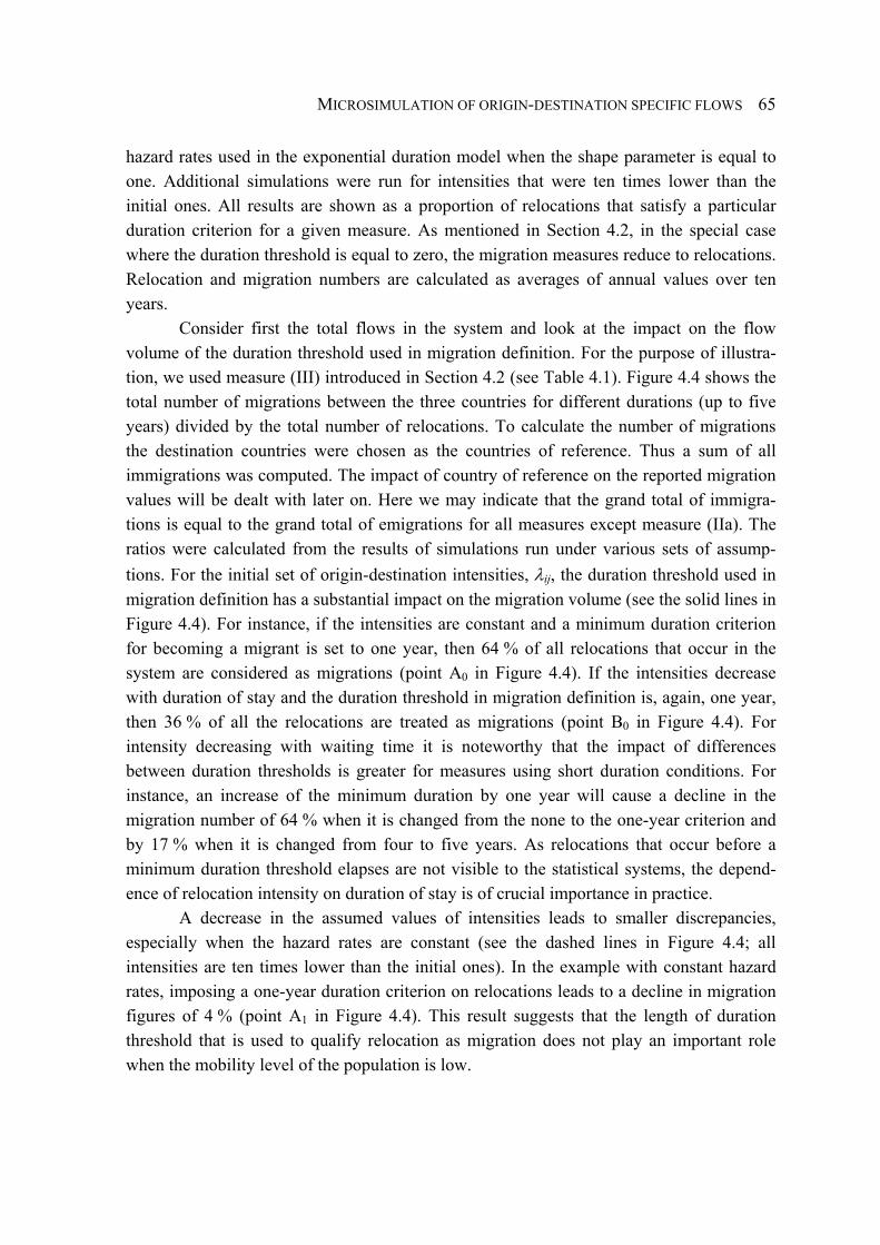
MICROSIMULATION OF ORIGIN-DESTINATION SPECIFIC FLOWS
65
hazard rates used in the exponential duration model when the shape parameter is equal to one. Additional simulations were run for intensities that were ten times lower than the initial ones. All results are shown as a proportion of relocations that satisfy a particular duration criterion for a given measure. As mentioned in Section 4.2, in the special case where the duration threshold is equal to zero, the migration measures reduce to relocations. Relocation and migration numbers are calculated as averages of annual values over ten years. Consider first the total flows in the system and look at the impact on the flow volume of the duration threshold used in migration definition. For the purpose of illustra-tion, we used measure (III) introduced in Section 4.2 (see Table 4.1). Figure 4.4 shows the total number of migrations between the three countries for different durations (up to five years) divided by the total number of relocations. To calculate the number of migrations the destination countries were chosen as the countries of reference. Thus a sum of all immigrations was computed. The impact of country of reference on the reported migration values will be dealt with later on. Here we may indicate that the grand total of immigra-tions is equal to the grand total of emigrations for all measures except measure (IIa). The ratios were calculated from the results of simulations run under various sets of assump-tions. For the initial set of origin-destination intensities, λij, the duration threshold used in migration definition has a substantial impact on the migration volume (see the solid lines in Figure 4.4). For instance, if the intensities are constant and a minimum duration criterion for becoming a migrant is set to one year, then 64 % of all relocations that occur in the system are considered as migrations (point A0 in Figure 4.4). If the intensities decrease with duration of stay and the duration threshold in migration definition is, again, one year, then 36 % of all the relocations are treated as migrations (point B0 in Figure 4.4). For intensity decreasing with waiting time it is noteworthy that the impact of differences between duration thresholds is greater for measures using short duration conditions. For instance, an increase of the minimum duration by one year will cause a decline in the migration number of 64 % when it is changed from the none to the one-year criterion and by 17 % when it is changed from four to five years. As relocations that occur before a minimum duration threshold elapses are not visible to the statistical systems, the depend-ence of relocation intensity on duration of stay is of crucial importance in practice. A decrease in the assumed values of intensities leads to smaller discrepancies, especially when the hazard rates are constant (see the dashed lines in Figure 4.4; all intensities are ten times lower than the initial ones). In the example with constant hazard rates, imposing a one-year duration criterion on relocations leads to a decline in migration figures of 4 % (point A1 in Figure 4.4). This result suggests that the length of duration threshold that is used to qualify relocation as migration does not play an important role when the mobility level of the population is low.
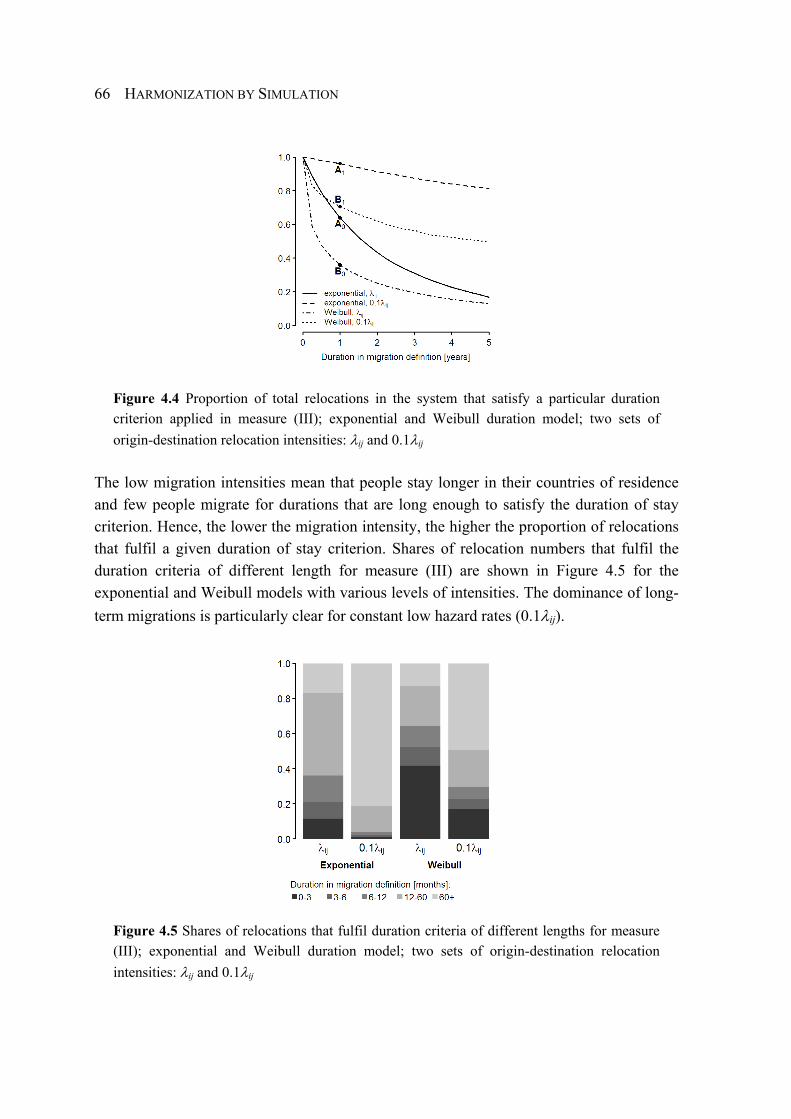
HARMONIZATION BY SIMULATION
66
Figure 4.4 Proportion of total relocations in the system that satisfy a particular duration criterion applied in measure (III); exponential and Weibull duration model; two sets of origin-destination relocation intensities: λij and 0.1λij
The low migration intensities mean that people stay longer in their countries of residence and few people migrate for durations that are long enough to satisfy the duration of stay criterion. Hence, the lower the migration intensity, the higher the proportion of relocations that fulfil a given duration of stay criterion. Shares of relocation numbers that fulfil the duration criteria of different length for measure (III) are shown in Figure 4.5 for the exponential and Weibull models with various levels of intensities. The dominance of long-term migrations is particularly clear for constant low hazard rates (0.1λij).
Figure 4.5 Shares of relocations that fulfil duration criteria of different lengths for measure (III); exponential and Weibull duration model; two sets of origin-destination relocation intensities: λij and 0.1λij
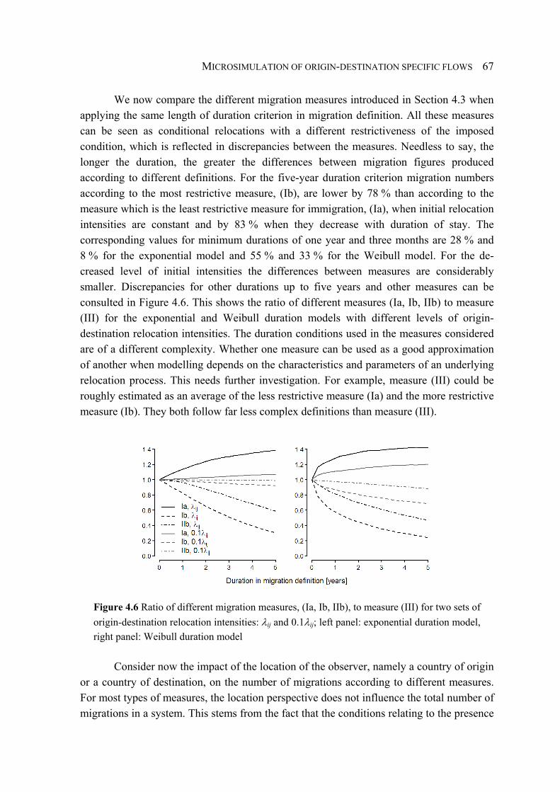
MICROSIMULATION OF ORIGIN-DESTINATION SPECIFIC FLOWS
67
We now compare the different migration measures introduced in Section 4.3 when applying the same length of duration criterion in migration definition. All these measures can be seen as conditional relocations with a different restrictiveness of the imposed condition, which is reflected in discrepancies between the measures. Needless to say, the longer the duration, the greater the differences between migration figures produced according to different definitions. For the five-year duration criterion migration numbers according to the most restrictive measure, (Ib), are lower by 78 % than according to the measure which is the least restrictive measure for immigration, (Ia), when initial relocation intensities are constant and by 83 % when they decrease with duration of stay. The corresponding values for minimum durations of one year and three months are 28 % and 8 % for the exponential model and 55 % and 33 % for the Weibull model. For the de-creased level of initial intensities the differences between measures are considerably smaller. Discrepancies for other durations up to five years and other measures can be consulted in Figure 4.6. This shows the ratio of different measures (Ia, Ib, IIb) to measure (III) for the exponential and Weibull duration models with different levels of origin-destination relocation intensities. The duration conditions used in the measures considered are of a different complexity. Whether one measure can be used as a good approximation of another when modelling depends on the characteristics and parameters of an underlying relocation process. This needs further investigation. For example, measure (III) could be roughly estimated as an average of the less restrictive measure (Ia) and the more restrictive measure (Ib). They both follow far less complex definitions than measure (III).
Figure 4.6 Ratio of different migration measures, (Ia, Ib, IIb), to measure (III) for two sets of origin-destination relocation intensities: λij and 0.1λij; left panel: exponential duration model, right panel: Weibull duration model
Consider now the impact of the location of the observer, namely a country of origin or a country of destination, on the number of migrations according to different measures. For most types of measures, the location perspective does not influence the total number of migrations in a system. This stems from the fact that the conditions relating to the presence
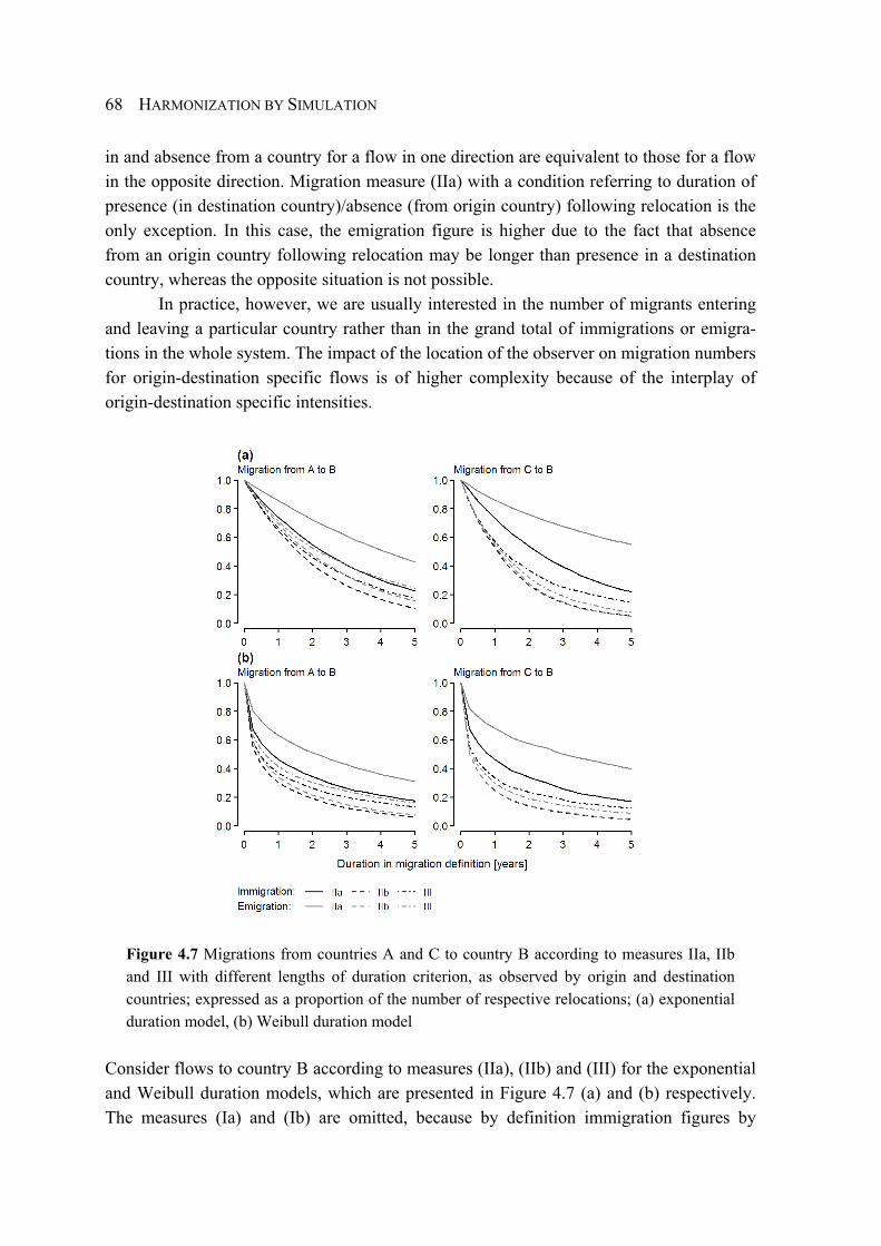
HARMONIZATION BY SIMULATION
68
in and absence from a country for a flow in one direction are equivalent to those for a flow in the opposite direction. Migration measure (IIa) with a condition referring to duration of presence (in destination country)/absence (from origin country) following relocation is the only exception. In this case, the emigration figure is higher due to the fact that absence from an origin country following relocation may be longer than presence in a destination country, whereas the opposite situation is not possible. In practice, however, we are usually interested in the number of migrants entering and leaving a particular country rather than in the grand total of immigrations or emigra-tions in the whole system. The impact of the location of the observer on migration numbers for origin-destination specific flows is of higher complexity because of the interplay of origin-destination specific intensities.
Figure 4.7 Migrations from countries A and C to country B according to measures IIa, IIb and III with different lengths of duration criterion, as observed by origin and destination countries; expressed as a proportion of the number of respective relocations; (a) exponential duration model, (b) Weibull duration model
Consider flows to country B according to measures (IIa), (IIb) and (III) for the exponential and Weibull duration models, which are presented in Figure 4.7 (a) and (b) respectively. The measures (Ia) and (Ib) are omitted, because by definition immigration figures by
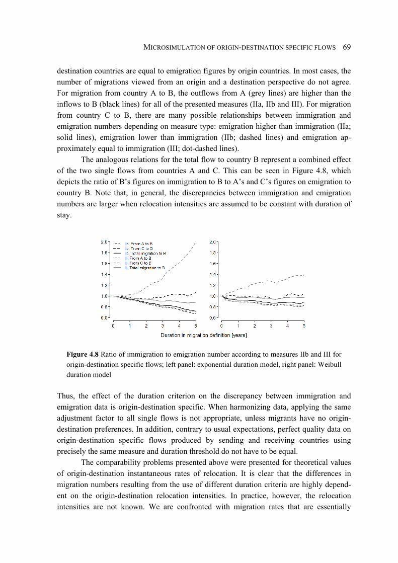
MICROSIMULATION OF ORIGIN-DESTINATION SPECIFIC FLOWS
69
destination countries are equal to emigration figures by origin countries. In most cases, the number of migrations viewed from an origin and a destination perspective do not agree. For migration from country A to B, the outflows from A (grey lines) are higher than the inflows to B (black lines) for all of the presented measures (IIa, IIb and III). For migration from country C to B, there are many possible relationships between immigration and emigration numbers depending on measure type: emigration higher than immigration (IIa; solid lines), emigration lower than immigration (IIb; dashed lines) and emigration ap-proximately equal to immigration (III; dot-dashed lines).
The analogous relations for the total flow to country B represent a combined effect of the two single flows from countries A and C. This can be seen in Figure 4.8, which depicts the ratio of B’s figures on immigration to B to A’s and C’s figures on emigration to country B. Note that, in general, the discrepancies between immigration and emigration numbers are larger when relocation intensities are assumed to be constant with duration of stay.
Figure 4.8 Ratio of immigration to emigration number according to measures IIb and III for origin-destination specific flows; left panel: exponential duration model, right panel: Weibull duration model
Thus, the effect of the duration criterion on the discrepancy between immigration and emigration data is origin-destination specific. When harmonizing data, applying the same adjustment factor to all single flows is not appropriate, unless migrants have no origin-destination preferences. In addition, contrary to usual expectations, perfect quality data on origin-destination specific flows produced by sending and receiving countries using precisely the same measure and duration threshold do not have to be equal. The comparability problems presented above were presented for theoretical values of origin-destination instantaneous rates of relocation. It is clear that the differences in migration numbers resulting from the use of different duration criteria are highly depend-ent on the origin-destination relocation intensities. In practice, however, the relocation intensities are not known. We are confronted with migration rates that are essentially

HARMONIZATION BY SIMULATION
70
conditional rates of relocation. The challenge, and a subject of future research, is to express one rate in terms of the other. Figure 4.9 illustrates the problem and shows the conditional rates of relocation estimated using the time to events considered as migration under measure (III). For longer durations they are substantially lower than relocation rates.
Figure 4.9 Emigration rates estimated from simulated relocations counted as migrations according to measure (III); left panel: exponential duration model, right panel: Weibull duration model, estimation under the assumption of constant hazard rates
If conditional rates are used for the harmonization of the available data instead of uncondi-tional ones the adjustment factors are underestimated. In addition, further disturbances are caused by the fact that conditional relocation rates differ even if the unconditional rates are the same, as is visible in Figure 4.9.
4.5. Conclusions
The complexity of the migration process poses a considerable challenge to providing an unambiguous definition of migration that could be successfully applied in practice. As a result, there are various definitions with multiple possible interpretations. Therefore, it should not come as a surprise that the emigration figure reported by a country of origin for a particular origin-destination flow does not usually agree with the immigration figure produced by a country of destination. The most common explanations given for the existing discrepancies are differences in migration definitions applied by those countries and measurement errors. The minimum duration threshold for becoming a migrant has, however, implications that are not obvious but that are important for the comparison of flows recorded by different countries. First, for most measures origin-destination migration paths of individuals are not consistent in terms of direction of migration. For instance, the statistics may indicate that a person migrates in exactly the same direction a few times in a

MICROSIMULATION OF ORIGIN-DESTINATION SPECIFIC FLOWS
71
row. Thus, being in a particular country and at the same time at risk of migrating to another one is ambiguous. Second, immigration and emigration figures reported for precisely the same flow do not have to be equal, even if the data are of perfect quality. This is because the length of presence in a destination country may differ from the length of absence from an origin country. All types of migration measures may be seen, however, as a conditional relocation with a different strictness of the imposed conditions. The strength of the conditions is reflected in the relationship between different measures when precisely the same minimum duration threshold is used in the definition of migration. Differences in the threshold cause further disturbances with their impact depending on the level of origin-destination relocation intensities and changes in them occurring with the increasing duration of stay in the country. It is also notable that origin-destination specific intensities lead to origin-destination specific discrepancies between immigration and emigration data. In general, all types of discrepancies between different measures are sensitive to the characteristics of relocation intensities. Thus, the knowledge of origin-destination relocation intensities is crucial for the harmonization of migration data. Future research should therefore pay adequate attention to their estimation methods.
References
Boyle P, Halfacree K, V R. 1998. Exploring Contemporary Migration. Longman: London.
Courgeau D. 2006. Mobility and spatial heterogeneity. In Demography: Analysis and Synthesis, Caselli G, Vallin J, Wunsch G (eds.); Vol. IV Academic Press-Elsevier: San Diego; 279-291.
Courgeau D. 1993. Measuring flows and stocks of internal migrants: Selected statistical issues. In Readings in Population Research Methodology, Bogue DJ, Arriaga EE, Anderton DL (eds.); Vol. 4 United Nations Fund for Population Activities: New York; 50-65.
European Commission. 2007. Regulation (EC) No 862/2007 of the European Parliament and of the Council of 11 July 2007 on Community statistics on migration and international protection. European Commission: Brussels. Available at: http://eur-lex.europa.eu/LexUriServ/LexUri Serv.do?uri=OJ:L:2007:199:0023:0029:EN:PDF [accessed 10 April 2010].
Kitsul P, Philipov D. 1981. The one-year/five-year migration problem. In Advances in Multire-gional Demography, Rogers A (ed.); International Institute for Applied Systems Analysis: Research Report RR-81-6, Laxenburg: Austria; 1-33.
Kraly EP, Warren R. 1992. Estimates of Long-Term Immigration to the United States: Moving US Statistics toward United Nations Concepts. Demography 29:613-626.
Kupiszewska D, Nowok B. 2008. Comparability of statistics on international migration flows in the European Union. In International Migration in Europe: Data, Models and Estimates, Raymer J, Willekens F (eds.); John Wiley & Sons, Ltd: Chichester; 41-71.
HARMONIZATION BY SIMULATION
72
Liaw KL. 1984. Interpolation of transition matrices by the variable power method. Environment and Planning A 16:917-925.
Long JF, Boertlein CG. 1990. Comparing migration measures having different intervals. Current Population Reports, Series P-23, No.166, U.S. Census Bureau: Washington.
Newbold KB. 2001. Counting Migrants and Migrations: Comparing Lifetime and Fixed-Interval Return and Onward Migration. Economic Geography 77:23-40.
Nowok B, Kupiszewska D, Poulain M. 2006. Statistics on international migration flows. In THESIM: Towards Harmonised European Statistics on International Migration, Poulain M, Perrin N, Singleton A (eds.); Presses Universitaires de Louvain: Louvain-la-Neuve; 203-231.
Poulain M, Dal L. 2008. Estimation of flows within the intra-EU migration matrix. GéDap-UCL, Discussion paper.
R Development Core Team. 2009. R: A language and environment for statistical computing. Vienna, Austria: R Foundation for Statistical Computing. Available at http://www.R-project. org.
Raymer J. 2007. The estimation of international migration flows: a general technique that focuses on the origin-destination association structure. Environment and Planning A 39:985-995.
Raymer J, Abel G. 2008. Review and improvement of estimation model developed in Task 2 (OD matrix for totals), 2002-2006. Deliverable 5.1 of the MIMOSA project, 26 May.
Rees P. 1977. The measurement of migration, from census data and other sources. Environment and Planning A 9:247-272.
Rogers A. 2008. Demographic Modeling of the Geography of Migration and Population: A Multiregional Perspective. Geographical Analysis 40:276-296.
Rogers A, Raymer J, Newbold KB. 2003. Reconciling and translating migration data collected over time intervals of differing widths. Annals of Regional Science 37:581-601.
Rogerson PA. 1990. Migration analysis using data with time intervals of differing widths. Papers in Regional Science 68:97-106.
Ross SM. 2006. Simulation. Academic Press.
Tuma NB, Hannan MT. 1984. Social Dynamics: Models and Methods. Academic Press: London.
United Nations. 1998. Recommendations on Statistics of International Migration: Revision 1. Statistical Papers, No. 58, Rev.1 Sales No. E.98.XVII.14: New York.
Willekens F. 1999. Modeling approaches to the indirect estimation of migration flows: from entropy to EM. Mathematical Population Studies 7:239-278.
Willekens F. 1985. Comparability of migration data: Utopia or reality? In Migrations Internes, Collecte Des Données Et Méthodes d'Analyse, Poulain M (ed.); Cabay: Louvain-la-Neuve; 409-441.
Willekens F. 1982. Identification and measurement of spatial population movements. In A National Migration Survey, Manual X: Guidelines for Analysis, United Nations ESCAP: New York; 74-97.
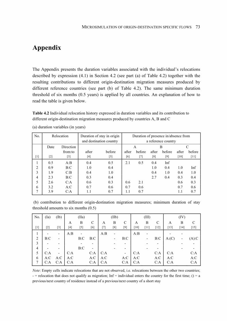
MICROSIMULATION OF ORIGIN-DESTINATION SPECIFIC FLOWS
73
Appendix
The Appendix presents the duration variables associated with the individual’s relocations described by expression (4.1) in Section 4.2 (see part (a) of Table 4.2) together with the resulting contributions to different origin-destination migration measures produced by different reference countries (see part (b) of Table 4.2). The same minimum duration threshold of six months (0.5 years) is applied by all countries. An explanation of how to read the table is given below.
Table 4.2 Individual relocation history expressed in duration variables and its contribution to different origin-destination migration measures produced by countries A, B and C
(a) duration variables (in years)
No. Relocation Duration of stay in origin and destination country
Duration of presence in/absence from a reference country
Date Direction A B C from:to after before after before after before after before
[1] [2] [3] [4] [5] [6] [7] [8] [9] [10] [11]
1 0.5 A:B 0.4 0.5 2.1 0.5 0.4 Inf 2 0.9 B:C 1.0 0.4 1.0 0.4 1.0 Inf 3 1.9 C:B 0.4 1.0 0.4 1.0 0.4 1.0 4 2.3 B:C 0.3 0.4 2.7 0.4 0.3 0.4 5 2.6 C:A 0.6 0.3 0.6 2.1 0.6 0.3 6 3.2 A:C 0.7 0.6 0.7 0.6 0.7 0.6 7 3.9 C:A 1.1 0.7 1.1 0.7 1.1 0.7
(b) contribution to different origin-destination migration measures; minimum duration of stay threshold amounts to six months (0.5)
No. (Ia) (Ib) (IIa) (IIb) (III) (IV) A B C A B C A B C A B C
[1] [2] [3] [4] [5] [6] [7] [8] [9] [10] [11] [12] [13] [14] [15]
1 - - A:B - A:B - A:B - - - 2 B:C - B:C B:C - B:C - B:C A:(C) - (A):C 3 - - - - - - - - - - 4 - - B:C - - - - - - - 5 C:A - C:A C:A C:A - C:A C:A C:A C:A 6 A:C A:C A:C A:C A:C A:C A:C A:C A:C A:C 7 C:A C:A C:A C:A C:A C:A C:A C:A C:A C:A
Note: Empty cells indicate relocations that are not observed, i.e. relocations between the other two countries; - = relocation that does not qualify as migration; Inf = individual enters the country for the first time; () = a previous/next country of residence instead of a previous/next country of a short stay
HARMONIZATION BY SIMULATION
74
The individual in question experiences seven relocations at the dates indicated in column 2. Consider the first relocation (line 1, unless otherwise indicated) from country A to country B (A:B) and taking place at time 0.5 ((a) column 2). Before relocation the person spends half a year in A ((a) column 5) and then moves to B, where he or she spends less than five months ((a) column 4). Thus, the duration of stay (episode) following relocation is shorter than the minimum threshold of six months and this relocation is not a migration according to measures (Ia) and (Ib) ((b) columns 2 and 3). Nonetheless, he or she relocates later on between B and C and comes back to A only at time 2.6 ((a) column 2). The person is therefore absent for 2.1 years ((a) column 6: 2.1, based on column 2, lines 5 and 1 respec-tively: 2.6-0.5=2.1) from A after his or her first observed relocation, which means the relocation qualifies as a migration according to measures (IIa) and (IIb), but only from the perspective of country A ((b) columns 4 and 7). The duration of presence in country B is too short to consider this relocation as a migration ((b) columns 5 and 8).
55
5. Reconciliation of migration measures by linking migration flows and population stocks
Abstract. International migration is by far the most complicated component of population change to measure and model. This chapter highlights the sheer complexity of origin-destination migration dynamics and difficulties with the specification of the migration process within the framework of a time-continuous Markov chain model. We describe the meaning of migration definition in the context of the relationship between migration flows and population stocks. The link between the two is crucial for calculating the occurrence/exposures rates that are widely used in demography.
5.1. Introduction
The data issues that confront international migration researchers become evident when a matrix of origin-destination migration flows between a set of countries is to be provided. The emigration figures produced by origin countries tend to differ, sometimes considera-bly, from immigration figures reported by destination countries. The first comparison of the statistics for the same migration flow which were produced by the sending and receiving countries was made for ECE countries for the year 1972 on the initiative of the Conference of European Statisticians. The 1972 double-entry matrix, which can be consulted in United Nations (1978:16), revealed the serious lack of data comparability. This encouraged further work on improving the quality of statistics on international migration flows. These efforts notwithstanding, the evidence that there were still inconsis-

HARMONIZATION BY SIMULATION
76
tencies for some later years is documented in the literature (Kelly, 1987; Kupiszewska and Nowok, 2008; Nowok et al., 2006; Poulain, 1999). The attempts to produce a consistent origin-destination migration flow matrix focused in general on using good quality data to correct inadequate data (Poulain, 1999; Poulain and Dal, 2008; Raymer and Abel, 2008). Note that the overall quality assessment of migration data has to be based, to a large extent, on expert opinion. The two main underlying sources of the discrepancies between figures on the same origin-destination migration flows that are published by sending and receiving countries are differences in the definition of migration and measurement errors. The latter encompasses all migration events that remain invisible in the data-collection process, regardless of the reason for this. Given the fact that measurement errors are hardly tractable, it seems reasonable to focus on the impact of definitions, in particular a mini-mum-duration-of-stay criterion that is usually used to qualify a change of country of residence as migration. Note that there is not necessarily one single correct or incorrect measure of international migration flows. The ultimate goal is therefore to develop a method for harmonizing the available data with any selected definition. Nonetheless, what is most desirable is the adjustment of the available data to the definition of long-term migration recommended by the United Nations (United Nations, 1998), which is essen-tially the same as the definition of migration required at the European Union level (Euro-pean Commission, 2007).
A starting and focal point of this chapter is the general notion that the different mi-gration measures produced in origin and destination countries represent observations of the same underlying relocation process. Differences in observations can be related to differ-ences in observation plan. A model of migration dynamics that takes the observational plan explicitly into account would be of considerable value. Since ‘human behaviour is reflected most easily in the specification of the state space and transition intensities’ (Hoem and Funck Jensen, 1982), the relocation intensities are the crucial elements of the model that needs to be estimated. The main goal of this chapter is to model origin-destination migration. Section 5.2 describes some specificities of the migration process and measures related to the dynamics of migration. Using simple examples, Section 5.3 presents a modelling approach that may be used as a starting point for future development. Section 5.4 concludes the chapter.
5.2. Model considerations
Migration by origin and destination can be represented by a time-continuous Markov process with a finite state space. The states of the Markov chain correspond to possible countries of residence. The time variable is the duration since a reference event. The dynamics of the process are determined by transition intensities. If we have complete
LINKING MIGRATION FLOWS AND POPULATION STOCKS
77
information on the migration histories of individuals including the exact timing of migra-tions, the intensities may be estimated by using well-known occurrence/exposure rates. These rates are the maximum likelihood estimators of the underlying theoretical transition intensities. The transition intensities are the fundamental quantities. Once they are available, all other typical quantities of interest can be computed. In studies of international migration serious difficulties arise in connection with an inherently vague concept of residence (Bilsborrow et al., 1997:18-21; United Nations, 1998). A duration criterion is usually given to clarify the definition of the event of migration, which basically refers to residential moves between countries. The duration threshold differs, sometimes considerably, from country to country. For instance, the United Nations defines migration as an action by which a person ‘moves to a country other than that of his or her usual residence for a period of at least a year (12 months)’ (United Nations, 1998). As a result, neither the occurrence of a migration event nor exposure to the risk of migration has a clear-cut meaning. The complexities of both components are presented below. The concept of relocation is consequently introduced. Relocation is a change of country of residence without any restriction on the duration of residence. The event of relocation has a clear-cut meaning. Migrations are conditional relocations. They are relocations that involve some degree of permanence. People who stay in a country for a short time are not immigrants. People who stay in a country for an extended time become usual residents and only those residents are at risk of emigration. International migration is a change from being a resident of country A to being a resident of country B. For that reason, the concept of migration is closely related to the concept of resident, and the harmonization of migration statistics should involve both flows and stocks. The duration criterion used in migration definition is also a membership criterion for a population. Immigration and emigration represent increments and decrements, respectively, to population size. An occurrence of migration from country A to country B decreases the population of country A and increases the population of country B. Conse-quently, at each point in time a person has one and only one country of usual residence. Despite the apparent simplicity, in practice there are many obstacles to establishing such a consistent and coherent framework for migration dynamics. This holds true even if we abstract from the fact that the duration threshold used in migration definition may differ between countries.
Suppose that all countries apply the same definition of migration recommended by the United Nations as quoted above. A move to and a three-month stay in a new country of usual residence is not treated as migration, but a return move followed by a stay of at least one year does qualify as migration. Some additional specifications are therefore needed in order to ensure that the trajectories of people’s unique countries of residence and changes thereto are complete and consistent in terms of direction. For instance, we may add an additional condition that a country becomes a new place of usual residence only once a person stays there for at least a year. Moreover, an origin of migration has to be a previous

HARMONIZATION BY SIMULATION
78
country of usual residence for at least one year and not a previous country of a ‘short’ usual residence. Consider now the time of migration. At the time of relocation, which should also be considered to be the time of potential migration, it is not known if the one-year duration condition will be satisfied. We can either rely on intentions or wait a year to check if the intentions are actually realized. Both options are acceptable, as is expressed directly in the European Union Regulation on Community statistics on migration and international protection. Duration criterion is specified as ‘a period that is, or is expected to be, of at least 12 months’ (European Commission, 2007). Note, however, that if occurrences refer to intended migrations, they may include some relocations for very short durations if intentions are not realized. Given the amended definition of migration presented above, let us look at the distribution of the total exposure time over the various countries of residence. Suppose that all intentions are realized and the actual duration is always equal to the intended one. A person becomes a usual resident of a destination country if he or she spends at least a year there. In other words, only individuals who survive a year are included in the official figures for the de jure population. They are included at the time of relocation. People who stay less than a year are completely invisible to the statistical system. Hence, they are present in the country and belong to the de facto population but they do not contribute to exposure time because they do not belong to the de jure population. Taking the perspective of an origin country, people who leave the country but return within a year are not excluded from the population. They are treated as if they had never left the origin popula-tion. They contribute neither to decrements nor to increments in the origin population. They must survive abroad for at least a year to be treated as return migrants when they come back. These individuals are continuous residents of the origin country, but at the same time they are not always ‘at risk’ of emigrating from the country in question in each direction. During their short stays abroad they cannot experience an emigration from the origin country to the country they are now in. They can, however, emigrate in other directions. Consider a resident of country A who moves to country B, stays in country B for a short time and then moves from country B to country C and resides there for more than one year. This person is a migrant from country A – a previous country of usual residence – to country C – a new country of usual residence. Note that during the stay in B, the usual resident of country A is at risk of migration, in other words of relocating and staying long enough to qualify as migrant, to country C only. The length of a short stay in country B should therefore be excluded from the exposure time to risk of emigration to country B. At the same time, he or she is at risk of relocation – changing de facto residence – to country A and to country C. Thus, only individuals who belong at a particular moment to both the de facto and the de jure population are at risk of relocation and migration from the country to all possible destination countries.

LINKING MIGRATION FLOWS AND POPULATION STOCKS
79
In the above considerations we assumed that all countries apply exactly the same definition of migration. Thus, they use the same threshold of length of stay following relocation that constitutes a new country of usual residence. As a result, there is a clear relationship between migration flows and population stocks. What if the duration criterion differs from country to country, which is usually the case in practice? Does it inevitably lead to inconsistencies between migration flows and population stocks? Consistency can be achieved by implementing a rule that a change of usual country of residence takes place only when an individual becomes a usual resident of a destination country. In other words, only a duration criterion used by the destination country is considered. This causes a lack of consistency between figures on migration flows for different directions. Nonetheless, a consistent system of migration flows and population stocks is more important than equality of origin-destination migration figures provided by a sending and receiving country that correspond neither to the population number of the origin country nor to the population number of the destination country. In general, steps towards the harmonization of data on migration dynamics should be taken for both flows and stocks at the same time. Note that such changes of usual country of residence are analogous to changes of citizenship, if dual citizenship is not allowed. A person becomes a citizen of a new country only if he or she renounces citizenship elsewhere. The rules of the new country of citizenship are binding.
A similar idea was implemented by the inter-Nordic agreement on population regis-tration, which applies to migrations between Denmark, Finland, Iceland, Norway and Sweden. The local registration authorities of the country of destination decide on the prerequisites of registration, which in practice means that the migration definition of the immigration country is used to produce migration statistics in both the sending and the receiving country. The data are transferred electronically between the registration authori-ties of the country of origin and the country of destination. The almost identical migration numbers produced by sending and receiving countries therefore does not come as a surprise.
This cannot be achieved in the absence of cooperation between origin and destina-tion countries and the coordination of registration systems. Therefore, different duration criteria used by countries to qualify relocation as migration lead in most cases to an increased level of complexity of stock and flow relationships in migration dynamics. It may be the case that an individual has no country of residence in some periods or has two countries of residence at the same time. In sum, occurrences of migration are conditional upon country of usual residence and upon what happens after a change of country of residence, and exposures do not correspond with the status defined as country of residence. These features are some of the most important aspects of the migration process that need to be captured in the model of migration dynamics. This task, however, is complex and certainly not trivial, especially when combined with the various duration thresholds that are used in migration definition in different countries.

HARMONIZATION BY SIMULATION
80
5.3. The maximum likelihood estimation of relocation intensities
The data on migration flows collected by different observational plans are manifestations of the same underlying relocation process. Knowledge of this process provides a basis for the calculation of various migration measures. The straightforward approach is to formu-late the likelihood of what is actually observed and to estimate the parameters of the process. Nonetheless, some observation plans lead to considerable complexity in the resulting measures when it comes to discrete time and difficulties with the formulation of a corresponding likelihood function. Note that individual relocation histories recorded in continuous time, which are best suited for estimates of relocation intensities, are not usually available. It is to be hoped that they will be more prevalent in the future. They are crucial, for instance, for properly capturing heterogeneity, impact of duration of stay or occurrence dependence. Currently, only origin-destination specific total flows tend to be produced on a yearly basis. For this many assumptions have to be made. Below we illustrate the modelling approach to the analysis of migration measures based on such aggregate data.
Consider first the total number of international migrations observed in a closed sys-tem of a few countries. The recorded figures include relocations that are followed by a minimum duration of stay, mt . We disregarded the direction of flows. In such a situation all
population members are permanently at risk of relocation (and migration) and they contribute to the exposure time. This example will illustrate, therefore, the complexities connected with occurrences of migrations, as opposed to relocations. Assume that the intensity of relocation λ does not vary with duration of residence. In other words, we assumed that for an individual the distribution of the number of occurrences of relocations in an interval of length t is well approximated by the Poisson distribution with an intensity parameter of λt. The parameter λ is the expected number of relocations in an interval of unit length. For a homogenous population, P, the relocation level is equal to Pλt.
Suppose that in a population of two thousand identical individuals (P=2000) we observe two hundred migrations (n=200) during a year (t=1). These migrations are changes of usual country of residence (relocations) that are followed by a stay of at least one year ( 1mt = ). Migration is a repeatable event. If we incorrectly treated the number of
migrations as a number of relocations, then we would use a standard likelihood function for a Poisson model
( ) ( ) ( )exp!
nP t P tLn
λ λλ −= , (5.1)
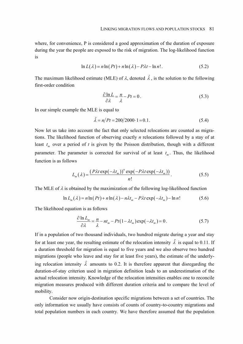
LINKING MIGRATION FLOWS AND POPULATION STOCKS
81
where, for convenience, P is considered a good approximation of the duration of exposure during the year the people are exposed to the risk of migration. The log-likelihood function is
( ) ( ) ( )ln ln ln ln !L n Pt n P t nλ λ λ= + − − . (5.2)
The maximum likelihood estimate (MLE) of λ, denoted λ̂ , is the solution to the following first-order condition
ln 0L n Ptλ λ
∂ = − =∂
. (5.3)
In our simple example the MLE is equal to
ˆ 200 2000 1 0.1n Ptλ = = ⋅ = . (5.4)
Now let us take into account the fact that only selected relocations are counted as migra-tions. The likelihood function of observing exactly n relocations followed by a stay of at least mt over a period of t is given by the Poisson distribution, though with a different
parameter. The parameter is corrected for survival of at least mt . Thus, the likelihood
function is as follows
( ) ( )( ) ( )( )exp exp exp!
nm m
mP t t P t tL
nλ λ λ λλ − − −
= . (5.5)
The MLE of λ is obtained by the maximization of the following log-likelihood function
( ) ( ) ( ) ( )ln ln ln exp ln !m m mL n Pt n n t P t t nλ λ λ λ λ= + − − − − (5.6)
The likelihood equation is as follows
( ) ( )ln 1 exp 0mm m m
L n nt Pt t tλ λλ λ
∂= − − − − =
∂. (5.7)
If in a population of two thousand individuals, two hundred migrate during a year and stay for at least one year, the resulting estimate of the relocation intensity λ̂ is equal to 0.11. If a duration threshold for migration is equal to five years and we also observe two hundred migrations (people who leave and stay for at least five years), the estimate of the underly-ing relocation intensity λ̂ amounts to 0.2. It is therefore apparent that disregarding the duration-of-stay criterion used in migration definition leads to an underestimation of the actual relocation intensity. Knowledge of the relocation intensities enables one to reconcile migration measures produced with different duration criteria and to compare the level of mobility. Consider now origin-destination specific migrations between a set of countries. The only information we usually have consists of counts of country-to-country migrations and total population numbers in each country. We have therefore assumed that the population
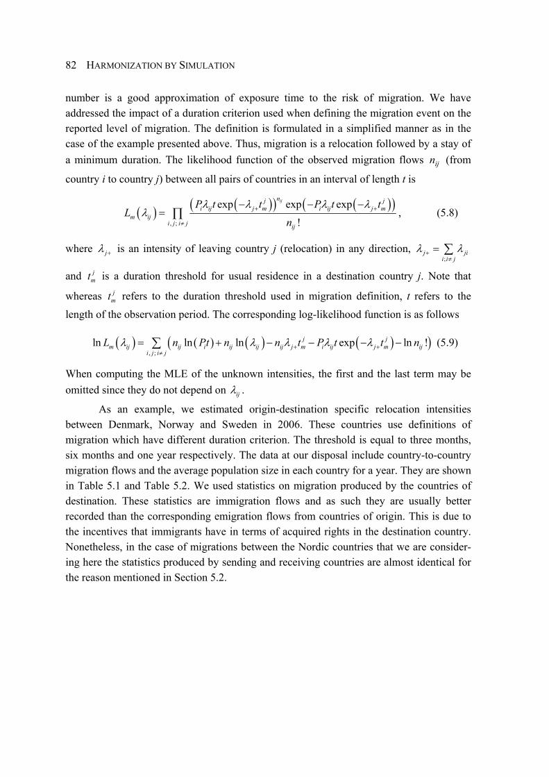
HARMONIZATION BY SIMULATION
82
number is a good approximation of exposure time to the risk of migration. We have addressed the impact of a duration criterion used when defining the migration event on the reported level of migration. The definition is formulated in a simplified manner as in the case of the example presented above. Thus, migration is a relocation followed by a stay of a minimum duration. The likelihood function of the observed migration flows ijn (from
country i to country j) between all pairs of countries in an interval of length t is
( ) ( )( ) ( )( ), ;
exp exp exp
!
ijnj ji ij j m i ij j m
m iji j i j ij
P t t P t tL
n
λ λ λ λλ + +
≠
− − −= ∏ , (5.8)
where jλ + is an intensity of leaving country j (relocation) in any direction, ;
j jii i j
λ λ+≠
= ∑
and jmt is a duration threshold for usual residence in a destination country j. Note that
whereas jmt refers to the duration threshold used in migration definition, t refers to the
length of the observation period. The corresponding log-likelihood function is as follows
( ) ( ) ( ) ( )( ), ;
ln ln ln exp ln !j jm ij ij i ij ij ij j m i ij j m ij
i j i jL n Pt n n t P t t nλ λ λ λ λ+ +
≠= + − − − −∑ (5.9)
When computing the MLE of the unknown intensities, the first and the last term may be omitted since they do not depend on ijλ .
As an example, we estimated origin-destination specific relocation intensities between Denmark, Norway and Sweden in 2006. These countries use definitions of migration which have different duration criterion. The threshold is equal to three months, six months and one year respectively. The data at our disposal include country-to-country migration flows and the average population size in each country for a year. They are shown in Table 5.1 and Table 5.2. We used statistics on migration produced by the countries of destination. These statistics are immigration flows and as such they are usually better recorded than the corresponding emigration flows from countries of origin. This is due to the incentives that immigrants have in terms of acquired rights in the destination country. Nonetheless, in the case of migrations between the Nordic countries that we are consider-ing here the statistics produced by sending and receiving countries are almost identical for the reason mentioned in Section 5.2.
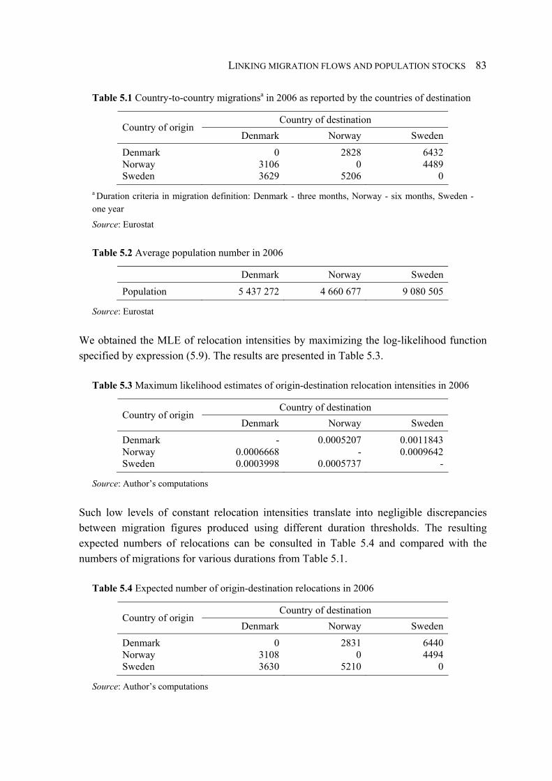
LINKING MIGRATION FLOWS AND POPULATION STOCKS
83
Table 5.1 Country-to-country migrationsa in 2006 as reported by the countries of destination
Country of destination Country of origin
Denmark Norway Sweden
Denmark 0 2828 6432 Norway 3106 0 4489 Sweden 3629 5206 0
a Duration criteria in migration definition: Denmark - three months, Norway - six months, Sweden - one year
Source: Eurostat
Table 5.2 Average population number in 2006
Denmark Norway Sweden
Population 5 437 272 4 660 677 9 080 505
Source: Eurostat
We obtained the MLE of relocation intensities by maximizing the log-likelihood function specified by expression (5.9). The results are presented in Table 5.3.
Table 5.3 Maximum likelihood estimates of origin-destination relocation intensities in 2006
Country of destination Country of origin
Denmark Norway Sweden
Denmark - 0.0005207 0.0011843 Norway 0.0006668 - 0.0009642 Sweden 0.0003998 0.0005737 -
Source: Author’s computations
Such low levels of constant relocation intensities translate into negligible discrepancies between migration figures produced using different duration thresholds. The resulting expected numbers of relocations can be consulted in Table 5.4 and compared with the numbers of migrations for various durations from Table 5.1.
Table 5.4 Expected number of origin-destination relocations in 2006
Country of destination Country of origin
Denmark Norway Sweden
Denmark 0 2831 6440 Norway 3108 0 4494 Sweden 3630 5210 0
Source: Author’s computations
HARMONIZATION BY SIMULATION
84
Note that the very limited impact of duration threshold on migration numbers results, to a large extent, from the simplified assumptions about the relocation process that ignore the effect of duration of stay, occurrence dependence and population heterogeneity.
5.4. Conclusions
When studying the dynamics of international migration, the most basic question that needs addressing is how many people migrate from country to country. In the presence of various concepts and measures of migration there is no easy answer to this question. In order to obtain a clear and satisfactory answer we need a consistent system that ensures that those moving between the countries belong to the population of only one country at any one time and that prevents a scenario where movers are not included in any population. Conse-quently, migration is a change of population membership and ideally the membership criteria should be the same in all countries. We should therefore aim to answer our basic question within this model framework. The equality of migration figures reported by origin and destination country is not an ultimate goal. Nevertheless, we should carry out gradual improvements and obtain the best possible estimates, given the available data. The data are the result of the observation of the underlying relocation processes. The relocation intensities are therefore crucial in modelling migration dynamics and reconciling various measures of migration.
References
Bilsborrow RE, Hugo G, Oberai AS, Zlotnik H. 1997. International Migration Statistics: Guide-lines for Improving Data Collection Systems. International Labour Office: Geneva.
European Commission. 2007. Regulation (EC) No 862/2007 of the European Parliament and of the Council of 11 July 2007 on Community statistics on migration and international protection. European Commission: Brussels. Available at: http://eur-lex.europa.eu/LexUriServ/LexUri Serv.do?uri=OJ:L:2007:199:0023:0029:EN:PDF [accessed 10 April 2010].
Hoem JM, Funck Jensen U. 1982. Multistate life table methodology: A probabilist critique. In Multidimensional Mathematical Demography, Land K, Rogers A (eds.); Academic Press: New York; 155-264.
Kelly JJ. 1987. Improving the comparability of international migration statistics: contributions by the Conference of European Statisticians from 1971 to date. International Migration Review 21:1017-1037.

LINKING MIGRATION FLOWS AND POPULATION STOCKS
85
Kupiszewska D, Nowok B. 2008. Comparability of statistics on international migration flows in the European Union. In International Migration in Europe: Data, Models and Estimates, Raymer J, Willekens F (eds.); John Wiley & Sons, Ltd: Chichester; 41-71.
Nowok B, Kupiszewska D, Poulain M. 2006. Statistics on international migration flows. In THESIM: Towards Harmonised European Statistics on International Migration, Poulain M, Perrin N, Singleton A (eds.); Presses Universitaires de Louvain: Louvain-la-Neuve; 203-231.
Poulain M. 1999. International migration within Europe: towards more complete and reliable data? Paper presented at Joint ECE-Eurostat Work Session on Demographic Projections, Pe-rugia, May 1999.
Poulain M, Dal L. 2008. Estimation of flows within the intra-EU migration matrix. GéDap-UCL, Discussion paper.
Raymer J, Abel G. 2008. Review and improvement of estimation model developed in Task 2 (OD matrix for totals), 2002-2006. Deliverable 5.1 of the MIMOSA project, 26 May.
United Nations. 1998. Recommendations on Statistics of International Migration: Revision 1. Statistical Papers, No. 58, Rev.1 Sales No. E.98.XVII.14: New York.
United Nations. 1978. Statistics of International Migration, Demographic Yearbook 1977. UN Publication, Sales No. E/F.78.XIII.1: New York.


66
6. Analysis of data on origin-destination migration dynamics with R
Abstract. This chapter presents a collection of R functions that can be used to explore and analyze data on origin-destination migration flows. We aim to introduce the reader to simple routines developed in R that help to understand the complexities of migration data. The presented functions allow us to simulate origin-destination relocation trajectories and derive aggregate measures that are directly related to dynamics of international migration. The measures include number of migrations, which can be viewed as conditional relocations, number of transitions over a one-year period, population size and person-years lived during a one-year period. Some selected results of the functions are plotted to illustrate some useful graphics functionalities that are available in R.
6.1. Introduction
The aim of this chapter is to illustrate how R software can be used to facilitate the explora-tion and understanding of data on origin-destination migration flows. R is an open-source programming language and software environment for statistical computing and graphics (R Development Core Team, 2009). The presented routines, therefore, can be immediately implemented by anyone interested. The software and contributed extension packages are available from the Comprehensive R Archive Network (CRAN) repository, which can be found at http://cran.r-project.org/. The main R Web site, http://www.r-project.org, provides all essential information about R. It lists the on-line manuals, related books and other materials.

HARMONIZATION BY SIMULATION
88
We present a collection of R functions. One function simulates individual origin-destination relocation histories, where relocation is a change of a country of residence. The other functions produce aggregate measures related to origin-destination population dynamics. The basic measure is the number of migrations. Compared to defining reloca-tion, defining migration includes some additional conditions referring generally to duration of residence. A description of various migration definitions and their ambiguities can be found in Chapters 3 and 4 of this book.
All measures are compiled for the whole virtual population. Such aggregate data are usually available in practice. They should therefore be treated as an accessible basis for estimating the parameters of the underlying relocation processes. If estimates use the simulated numbers, the results should approximate the parameters of the process that was initially used to create relocation sample paths. The knowledge of the underlying processes provides a basis for deriving the requested migration measures.
A function for simulating relocation trajectories is described in Section 6.2. Func-tions for producing aggregate measures are the subject of Section 6.3. Section 6.4 includes a graphic presentation of some selected results of the functions. The last section concludes the chapter. A complete code for the functions and the example, together with some explanations, is provided in the Appendix.
6.2. Simulation
The aim of the simulation is to generate continuous-time relocation histories of individuals who may repeatedly relocate among a finite number of countries. The relocation paths are generated using the function simOD(). The simulation is carried out by determining the next transition times and the next states visited for all individuals in the initial population. The population numbers in each state at time zero are given in an argument vector Ni. An ending time of the observation is determined by tmax. For a given individual, the simulation terminates when the time of relocation occurrence is greater than tmax. The argument tdist specifies interarrival time distribution. The default exponen-tial distribution corresponds to tdist = "exp". Another possible choice is to assume that survival time follows a Weibull distribution and set tdist = "weibull". If an exponential model is assumed, the origin-destination relocation intensities are specified in matrix M. This matrix is organized so that rows correspond to origin countries and columns correspond to destination countries. The diagonal of the matrix is ignored. The dimensions of matrix M have to correspond to the number of considered countries. In the case of the Weibull distribution, a scale parameter is equal to an inverse of an appropriate transition intensity given in matrix M. A common shape parameter shapeWeibull has to be additionally specified.
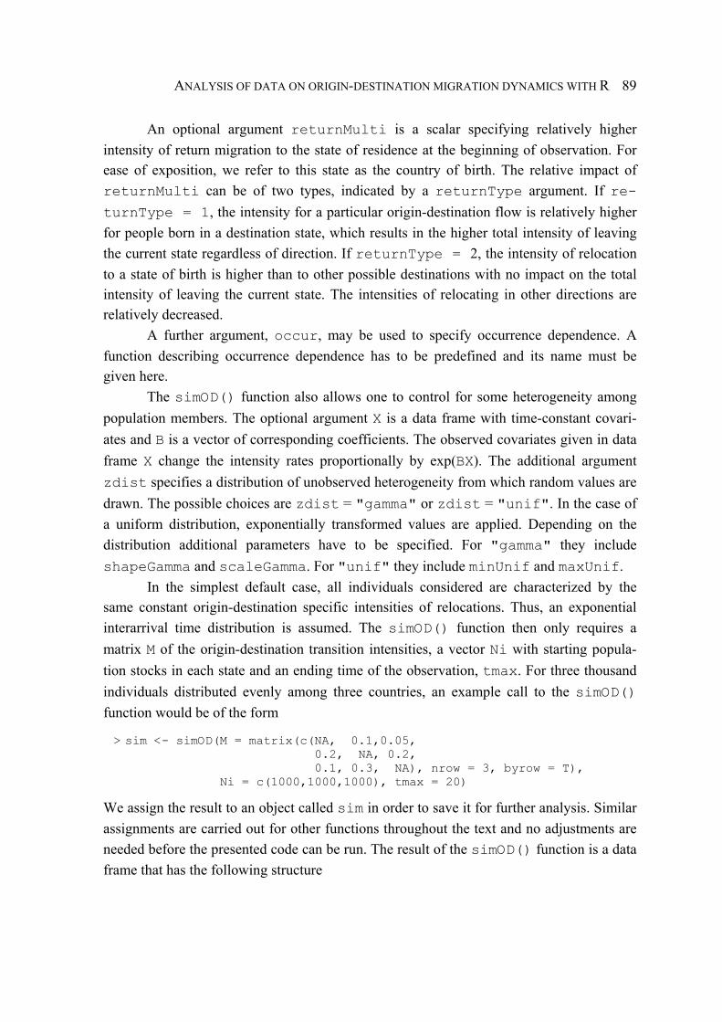
ANALYSIS OF DATA ON ORIGIN-DESTINATION MIGRATION DYNAMICS WITH R
89
An optional argument returnMulti is a scalar specifying relatively higher intensity of return migration to the state of residence at the beginning of observation. For ease of exposition, we refer to this state as the country of birth. The relative impact of returnMulti can be of two types, indicated by a returnType argument. If re-turnType = 1, the intensity for a particular origin-destination flow is relatively higher for people born in a destination state, which results in the higher total intensity of leaving the current state regardless of direction. If returnType = 2, the intensity of relocation to a state of birth is higher than to other possible destinations with no impact on the total intensity of leaving the current state. The intensities of relocating in other directions are relatively decreased. A further argument, occur, may be used to specify occurrence dependence. A function describing occurrence dependence has to be predefined and its name must be given here. The simOD() function also allows one to control for some heterogeneity among population members. The optional argument X is a data frame with time-constant covari-ates and B is a vector of corresponding coefficients. The observed covariates given in data frame X change the intensity rates proportionally by exp(BX). The additional argument zdist specifies a distribution of unobserved heterogeneity from which random values are drawn. The possible choices are zdist = "gamma" or zdist = "unif". In the case of a uniform distribution, exponentially transformed values are applied. Depending on the distribution additional parameters have to be specified. For "gamma" they include shapeGamma and scaleGamma. For "unif" they include minUnif and maxUnif. In the simplest default case, all individuals considered are characterized by the same constant origin-destination specific intensities of relocations. Thus, an exponential interarrival time distribution is assumed. The simOD() function then only requires a matrix M of the origin-destination transition intensities, a vector Ni with starting popula-tion stocks in each state and an ending time of the observation, tmax. For three thousand individuals distributed evenly among three countries, an example call to the simOD() function would be of the form
> sim <- simOD(M = matrix(c(NA, 0.1,0.05, 0.2, NA, 0.2, 0.1, 0.3, NA), nrow = 3, byrow = T), Ni = c(1000,1000,1000), tmax = 20)
We assign the result to an object called sim in order to save it for further analysis. Similar assignments are carried out for other functions throughout the text and no adjustments are needed before the presented code can be run. The result of the simOD() function is a data frame that has the following structure

HARMONIZATION BY SIMULATION
90
> sim ID time state 1 1 0.00 1 2 1 20.25 1 3 2 0.00 1 4 2 1.79 3 5 2 2.92 2 6 2 4.02 3 7 2 6.05 3 ...
For each individual distinguished by a unique identifier ID, it gives times of relocations (time) and countries of residence following relocations (state). The value of the state variable corresponding to time equal to zero refers to a country of residence at the beginning of the observation period. A country of residence at the end of the observa-tion period is indicated by state at time greater than tmax. For non-migrants it is the same as a country of residence at the onset of observation and for migrants it is a destina-tion country of the last observed relocation. If we control for heterogeneity across indi-viduals, the observed values of covariates or random values of unobserved heterogeneity are added to the final output of the function simOD() as additional columns in a data frame.
6.3. Migration measures
Aggregate measures are derived for the whole virtual population that is combined from the individual relocation histories generated by the simOD() function. We present functions that produce statistics that are directly related to the dynamics of international migration. The annual number of migrations (conditional relocations) is obtained using a migra-tions() function. It also returns individual trajectories of countries of de jure residence, which are utilized in other functions. A transitions() function produces the number of transitions over a one-year period, that is, the number of migrants that are usually estimated from a comparison of current country of residence and country of residence one year ago. A population() function returns population size and person-years lived during a year. All these functions use data argument, an output of the function si-mOD(). A second argument, tdef, is a vector of duration criteria expressed in years. These criteria refer to length of residence and they are used to distinguish migrations from relocations. Before we move on to a presentation of functions it is necessary to clarify the migration definition that is used in the example.
In order to ensure consistent and complete trajectories of unique countries of resi-dence and changes thereto, a migration is defined as a relocation that is followed by a continuous stay of a specified duration in a destination country, provided a person is a non-

ANALYSIS OF DATA ON ORIGIN-DESTINATION MIGRATION DYNAMICS WITH R
91
resident thereof. Thus, if an individual leaves his or her country of birth and then relocates a few times to different foreign countries, but does not reside long enough in any of them to become a migrant and thereby a member of the population, he or she remains an official (de jure) resident of the country of birth. This prevents the occurrence of a situation in which a person does not belong to any population. Note that a person has one unique place of residence only when all countries use the same minimum-duration threshold. The origin of migration is a previous country of residence and not a previous country of a short stay that does not constitute a residence.
The migrations() function produces residence histories of individuals and cal-culates the aggregate number of migrations as defined above. The result is a list of two components, ODmx and ODdata. ODmx is an array including annual origin-destination migration matrices for all years until tmax for all duration thresholds given in tdef. For simplicity, all countries use the same duration criterion. ODdata is a data frame that includes, inter alia, information on country of residence (ctr). If we only need the migration matrices we can use the following command
> M0 <- migrations(data = sim, tdef = seq(0,5,.05))$ODmx > M0
In order to decrease the execution time, the number of considered duration criteria can be limited to a few values, for instance, tdef = c(0,.25,.5,1). The definition of migration presented above leads to a straightforward correspond-ing measure of transitions. The transition is reflected in a different country of residence at the beginning and the end of the year. No additional duration criteria have to be applied. The transitions() function utilizes the migrations() function in order to obtain residence histories. This information is used to determine country of residence at the beginning and end of each year. Whereas the migration measure returned by migra-tions() represents an event approach to counting migration, the migration measure returned by transitions() represents a status approach. The output of the transi-tions() function has the same structure as the ODdata array from the output of the migrations() function. An example call to the transitions() function would be
> T0 <- transitions(data = sim, tdef = seq(0,5,.05)) > T0
The population size and person-years lived in the countries are obtained using the population()function, which could be called as follows
> P0 <- population(data = sim, tdef = seq(0,5,.05)) > P0
The output contains a list of three arrays with figures for each country (in columns) and each year (in rows). POP includes population numbers at the beginning of each year, POPavg gives an average annual population size and PY refers to the values of person-

HARMONIZATION BY SIMULATION
92
years. Note that different concepts of the population may be applied. Population size may refer to the total number of the residents irrespective of their current place of stay (de jure population). We can also count people present in the country irrespective of their countries of residence (de facto population). Both population numbers are returned by the popula-tion()function. They are denoted respectively by ctr and cts in the third dimension of output arrays POP and POPavg. In addition, population() gives the number of people who are present in their country of residence (ctrs). The person-years given in the array PY refers to the same population types as given in arrays POP and POPavg.
6.4. Plotting results
Once the relocation histories have been simulated and the migration measures have been compiled, any data of interest can be easily extracted for further analysis. The comprehen-sive graphics functionalities that are available in R play an indispensible facilitative role in the data exploration. Two illustrative examples are given below. In the first one, we compare the number of origin-destination specific migrations during a year with the number of corresponding transitions during a year. The figures are compared for the various lengths of duration criterion used to determine a country of residence. This duration threshold is the same for both types of measures of migration considered. In the second example, we look at person-years of residence in a given country and person-years of actual stay in that country of residence. For the three countries considered in the simulation there are six origin-destination specific migration flows. We do not consider flows within the countries. We aim to look at migration and transition counts for each of them. The Trellis graphics system with multipanel conditioning is particularly useful in such a case. It is provided in R in an add-on package called lattice. Before we can call a trellis function that is appropriate for plotting migrations and transitions against duration criterion as used in the definition and that is conditional on direction of flow, the data available in arrays M0 and T0 have to be arranged in one data frame. This can be easily done as follows
> M1 <- as.data.frame(as.table(M0)); M1$type <- "migrations" > T1 <- as.data.frame(as.table(T0)); T1$type <- "transitions" > MT <- rbind(M1, T1) > head(MT) from to year def Freq type 1 1 1 1 0 0 migrations 2 2 1 1 0 200 migrations 3 3 1 1 0 104 migrations 4 1 2 1 0 111 migrations 5 2 2 1 0 0 migrations 6 3 2 1 0 274 migrations
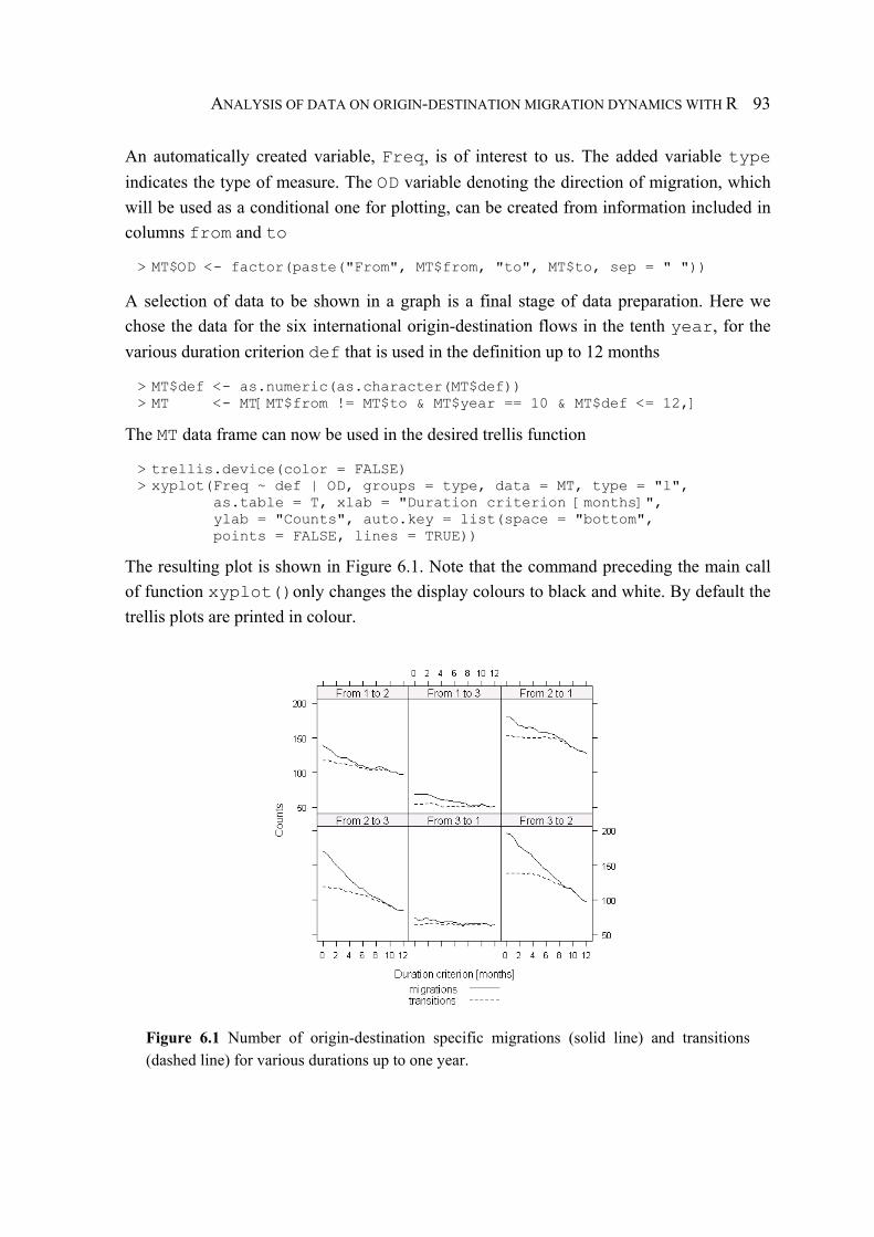
ANALYSIS OF DATA ON ORIGIN-DESTINATION MIGRATION DYNAMICS WITH R
93
An automatically created variable, Freq, is of interest to us. The added variable type indicates the type of measure. The OD variable denoting the direction of migration, which will be used as a conditional one for plotting, can be created from information included in columns from and to
> MT$OD <- factor(paste("From", MT$from, "to", MT$to, sep = " "))
A selection of data to be shown in a graph is a final stage of data preparation. Here we chose the data for the six international origin-destination flows in the tenth year, for the various duration criterion def that is used in the definition up to 12 months
> MT$def <- as.numeric(as.character(MT$def)) > MT <- MT[MT$from != MT$to & MT$year == 10 & MT$def <= 12,]
The MT data frame can now be used in the desired trellis function
> trellis.device(color = FALSE) > xyplot(Freq ~ def | OD, groups = type, data = MT, type = "l", as.table = T, xlab = "Duration criterion [months]", ylab = "Counts", auto.key = list(space = "bottom", points = FALSE, lines = TRUE))
The resulting plot is shown in Figure 6.1. Note that the command preceding the main call of function xyplot()only changes the display colours to black and white. By default the trellis plots are printed in colour.
Figure 6.1 Number of origin-destination specific migrations (solid line) and transitions (dashed line) for various durations up to one year.

HARMONIZATION BY SIMULATION
94
In the second example dealing with person-years for different population concepts, a subset of data can be obtained directly from the P0 array. The selection criteria are assigned to the following variables
> year <- 10 > state <- 2 > duration <- as.character(seq(0,5,.5))
For the chosen year, country (state) and duration thresholds of the person-years of resi-dence ctr can be presented in one bar plot together with the person-years actually spent in this country ctrs
> barplot(P0$PY[year, state, c("ctr","ctrs"), duration], beside = TRUE, space = c(-0.8,.4), las = 1, xlab = "Duration criterion [years]", ylab = "Person-years")
Figure 6.2 shows the obtained bar plot.
Figure 6.2 Person-years of residence (black bars) and person-years of actual stay in country of residence (grey bars) for various duration criteria in migration definition; country = 2, year = 10
The differences between the two data series indicate person-years spent by the individuals in the countries other than their place of residence.
6.5. Conclusions
This chapter has demonstrated a computer implementation of migration data analysis. The code was developed in the R environment, which has all the statistical, mathematical and graphical capabilities needed for exploring the data. The open-source nature of R offers obvious advantages. First, anyone interested can reproduce the analysis simply by re-executing the scripts. Second, the code can be easily modified to serve one’s needs better.

ANALYSIS OF DATA ON ORIGIN-DESTINATION MIGRATION DYNAMICS WITH R
95
Writing and documenting collections of R functions is, therefore, a very useful and effective way of organizing and communicating about the work.
References
R Development Core Team. 2009. R: A language and environment for statistical computing. Vienna, Austria: R Foundation for Statistical Computing. Available at http://www.R-project. org.
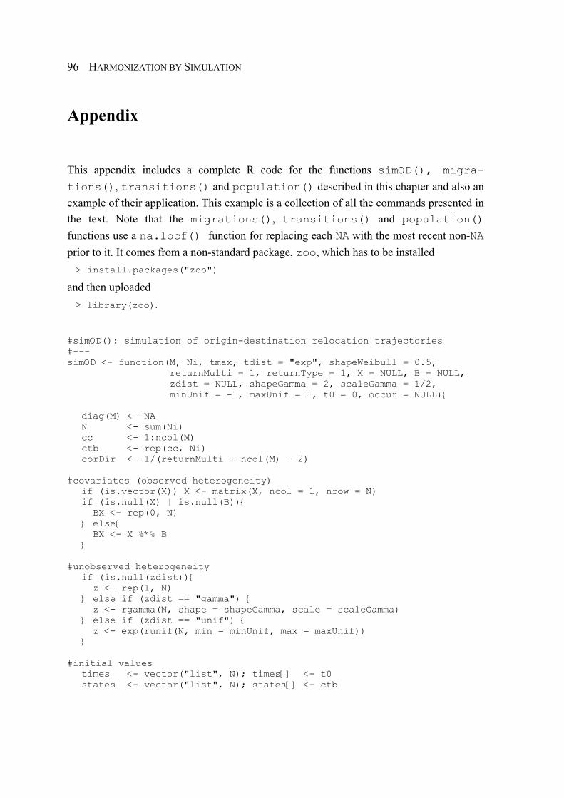
HARMONIZATION BY SIMULATION
96
Appendix
This appendix includes a complete R code for the functions simOD(), migra-
tions(), transitions() and population() described in this chapter and also an example of their application. This example is a collection of all the commands presented in the text. Note that the migrations(), transitions() and population() functions use a na.locf() function for replacing each NA with the most recent non-NA prior to it. It comes from a non-standard package, zoo, which has to be installed > install.packages("zoo")
and then uploaded > library(zoo).
#simOD(): simulation of origin-destination relocation trajectories #--- simOD <- function(M, Ni, tmax, tdist = "exp", shapeWeibull = 0.5, returnMulti = 1, returnType = 1, X = NULL, B = NULL, zdist = NULL, shapeGamma = 2, scaleGamma = 1/2, minUnif = -1, maxUnif = 1, t0 = 0, occur = NULL){ diag(M) <- NA N <- sum(Ni) cc <- 1:ncol(M) ctb <- rep(cc, Ni) corDir <- 1/(returnMulti + ncol(M) - 2)
#covariates (observed heterogeneity) if (is.vector(X)) X <- matrix(X, ncol = 1, nrow = N) if (is.null(X) | is.null(B)){ BX <- rep(0, N) } else{ BX <- X %*% B }
#unobserved heterogeneity if (is.null(zdist)){ z <- rep(1, N) } else if (zdist == "gamma") { z <- rgamma(N, shape = shapeGamma, scale = scaleGamma) } else if (zdist == "unif") { z <- exp(runif(N, min = minUnif, max = maxUnif)) }
#initial values times <- vector("list", N); times[] <- t0 states <- vector("list", N); states[] <- ctb

ANALYSIS OF DATA ON ORIGIN-DESTINATION MIGRATION DYNAMICS WITH R
97
###individual trajectories for (n in 1:N){ #impact of observed and unobserved heterogeneity on intensity M.n <- M*z[n]*exp(BX[n]) #increased intensity of return migration if (returnType == 1){ M.n[,ctb[n]] <- M.n[,ctb[n]] * returnMulti } else if (returnType == 2){ M.n[-ctb[n],] <- rep(corDir*rowSums(M.n[-ctb[n],], na.rm = T), ncol(M.n)) M.n[-ctb[n],ctb[n]] <- returnMulti*M.n[-ctb[n],ctb[n]] diag(M.n) <- NA }
##timings of relocations and their directions i <- 0 t.cum <- 0 while (t.cum <= tmax) { i <- i+1 #possible destinations Sorig <- states[[n]][i] Sdest <- cc[-Sorig] #occurrence dependence oc <- ifelse(is.null(occur), 1, eval(parse(text = occur))(i-1)) Rs <- oc*M.n[Sorig,Sdest]; k <- M[Sorig,Sdest]/Rs #waiting times to all possible destinations if(tdist == "exp"){ Ts <- rexp(length(cc)-1, rate = Rs) } else if (tdist == "weibull"){ Ts <- rweibull(length(cc)-1, shape = shapeWeibull, scale = 1/(Rs*k^(1/shapeWeibull-1))) } #minimum waiting time and a corresponding direction t.cum <- times[[n]][i] + min(Ts) times [[n]][i+1] <- t.cum states[[n]][i+1] <- ifelse(t.cum <= tmax, Sdest[which(Ts == min(Ts))], states[[n]][i]) }
## ### }
#output preparation ns <- unlist(lapply(states, length)) x <- unlist(times) y <- unlist(states) msmData <- cbind.data.frame(ID = rep(1:N, ns), time = x, state = y) if (!is.null(zdist)) msmData$z <- rep(z, ns) if (!is.null(X)){ msmCov <- matrix(ncol = ncol(X), nrow = sum(ns)) dimnames(msmCov)[[2]] <- as.list(paste("X", 1:ncol(X), sep = "")) for (i in 1:ncol(X)) msmCov[,i] <- rep(X[,i], ns) msmData <- cbind.data.frame(msmData, msmCov) } return(msmData)
} #--- #end of simOD()

HARMONIZATION BY SIMULATION
98
#migrations(): number of migrations for different duration #--- migrations <- function(data, tdef){ cc <- as.numeric(levels(factor(data$state))) ccNo <- length(cc) tmax <- floor(min(tapply(data$time, data$ID, max))) names(data)[3] <- "cts" OD.yy.def <- array(dim = c(ccNo, ccNo, tmax, length(tdef))) dimnames(OD.yy.def) <- list(from = cc, to = cc, year = 1:tmax, def = tdef*12) labvar <- c("ID","time","ctb","cts","ctr","mctr") ODdata <- array(dim = c(nrow(data), length(labvar), length(tdef)))
#country of birth data$ctb <- rep(data$cts[data$time == 0],table(data$ID))
#year of relocation data$year <- cut(data$time, c(0, 1:tmax), labels = FALSE)
#time till next (dnxt) and since previous (dprv) relocation data$dnxt <- c(diff(data$time), NA) data$dprv <- c(NA, diff(data$time)) data[which(data$time == 0 | data$time>=tmax), c("dnxt","dprv")] <- NA
#previous country of stay (pcts) data$pcts <- c(NA, data$cts[-length(data$cts)]) data$pcts[which(data$time == 0)] <- data$cts[data$time == 0]
#first relocation migs <- !is.na(data$dnxt) data$fst[migs] <- unlist(tapply(1:nrow(data[migs,]), data$ID[migs], seq_along)) data$dprv[data$pcts == data$ctb & data$fst == 1] <- 99
##migration counts for various duration criteria in definition for (t in 1:length(tdef)){ #relocations followed by a stay satisfying duration condition data$def.nxt <- cut(data$dnxt, c(tdef[t], Inf), labels = FALSE) durres <- which(data$def.nxt == 1) fstobs <- which(data$time == 0) #countries of residence (ctr) data$ctr <- NA data$ctr[durres] <- data$cts[durres] data$ctr[fstobs] <- data$ctb[fstobs] data$ctr <- na.locf(data$ctr) #previous countries of residence (pctr) data$pctr <- c(NA, data$ctr[-nrow(data)]) data$pctr[fstobs] <- data$ctr[fstobs] #migration as a change of country of residence (mctr) data$mctr <- as.numeric(!is.na(data$pctr) & data$pctr != data$ctr) data$mctr[data$mctr == 0] <- NA #origin-destination migration matrices OD.yy.def[,,,t] <- with(data, table(from = factor(pctr,cc), to = factor(ctr, cc), factor(year, levels = 1:tmax), mctr)) #output data frame with crucial variables ODdata[,,t] <- as.matrix(data[,labvar]) }
##

ANALYSIS OF DATA ON ORIGIN-DESTINATION MIGRATION DYNAMICS WITH R
99
dimnames(ODdata) <- list(1:nrow(ODdata), labvar, def = tdef*12) return(list(ODmx = OD.yy.def, ODdata = ODdata))
} #--- #end of migrations()
#transitions(): number of transitions over one year period #--- transitions <- function(data, tdef){ #country of residence in continuous time Ctr <- migrations(data = data, tdef = tdef)$ODdata cc <- as.numeric(levels(factor(data$state))) ccNo <- length(cc) tmax <- floor(min(tapply(data$time, data$ID, max))) cuts <- 1:tmax names(data)[3] <- "cts"
#country of birth data$ctb <- rep(data$cts[data$time == 0], table(data$ID)) IDs <- unique(data$ID)
#discrete time points (tPts) ID <- rep(IDs, each = length(cuts)) time <- rep(cuts, length(IDs)) tPts <- data.frame(ID, time) mTrans <- array(dim = c(ccNo, ccNo, tmax, length(tdef))) dimnames(mTrans) <- list(from = cc, to = cc, year = 1:tmax, def = tdef*12)
##transition counts for various duration criteria in definition for (t in 1:length(tdef)){ mig <- cbind(data, Ctr[,c("ctr","mctr"),t]) mig <- mig[mig$time <= tmax,] #country of residence at discrete time points obtained from #information on residence at continuous time points mD <- merge(mig, tPts, by = c("ID","time"), all = T) mD[,c("cts","ctb","ctr")] <- na.locf(mD[,c("cts","ctb","ctr")], na.rm = F) #country of residence at discrete time points (mD.yy) tpts <- mD$time %% 1 == 0 mD.yy <- mD[tpts,] #country of residence one year ago mD.yy$pctr <- c(NA, mD.yy$ctr[-nrow(mD.yy)]) mD.yy$pctr[mD.yy$time == 0] <- NA #transition - change of country of residence at discrete time points mD.yy$rtrans <- as.numeric(mD.yy$pctr != mD.yy$ctr) mD.yy$rtrans[mD.yy$rtrans == 0] <- NA #origin-destination transition matrices mTrans[,,,t] <- with(mD.yy, table(factor(pctr, levels = cc), factor(ctr, levels = cc), factor(time, levels = 1:tmax), rtrans)) }
## return(ODtrans = mTrans)
} #--- #end of transitions()

HARMONIZATION BY SIMULATION
100
#population(): population size and person-years #--- population <- function(data, tdef){ #country of residence in continuous time Ctr <- migrations(data = data, tdef = tdef)$ODdata cc <- levels(factor(data$state)) ccNo <- length(cc) tmax <- floor(min(tapply(data$time, data$ID, max))) cuts <- 1:tmax names(data)[3] <- "cts" data$ctb <- rep(data$cts[data$time == 0], table(data$ID)) IDs <- unique(data$ID) POP <- array(dim = c(tmax+1, ccNo, 3, length(tdef))) dimnames(POP) <- list(0:tmax, cc, country = c("ctr","cts","ctrs"), def = tdef) PY <- array(dim = c(tmax, ccNo, 3, length(tdef))) dimnames(PY) <- list(1:tmax, cc, country = c("ctr","cts","ctrs"), def = tdef)
#discrete time points ID <- rep(IDs, each = length(cuts)) time <- rep(cuts, length(IDs)) tPts <- data.frame(ID, time) for (t in 1:length(tdef)){ mig <- cbind(data, Ctr[,c("ctr","mctr"), t]) mig <- mig[mig$time <= tmax,] #time between relocations and discrete time points mD <- merge(mig, tPts, by = c("ID","time"), all = T) mD$year <- cut(mD$time, c(0,cuts), labels = FALSE, right = F) mD$tdif[mD$time != tmax] <- unlist(tapply(mD$time, mD$ID, diff)) mD[,c("cts","ctb","ctr")] <- na.locf(mD[,c("cts","ctb","ctr")], na.rm = F) #presence in country of residence (ctrs) mD$ctrs[mD$ctr == mD$cts] <- mD$ctr[mD$ctr == mD$cts] #person-years PY[,,"ctr",t] <- with(mD, tapply(tdif, list(year, factor(ctr, cc)), sum)) PY[,,"cts",t] <- with(mD, tapply(tdif, list(year, factor(cts, cc)), sum)) PY[,,"ctrs",t] <- with(mD, tapply(tdif, list(year, factor(ctrs,cc)), sum)) PY[is.na(PY)] <- 0 #population numbers at discrete time points tpts <- mD$time %% 1 == 0 mD.yy <- mD[tpts,] POP[,,"ctr",t] <- with(mD.yy, table(time, state = factor(ctr,cc))) POP[,,"cts",t] <- with(mD.yy, table(time, state = factor(cts,cc))) POP[,,"ctrs",t] <- with(mD.yy, table(time, state = factor(ctrs,cc))) POP[is.na(POP)] <- 0 }

ANALYSIS OF DATA ON ORIGIN-DESTINATION MIGRATION DYNAMICS WITH R
101
#average population number POPavg <- (POP[-1,,,] + POP[-nrow(POP),,,]) / 2 return(list(POP = POP, POPavg = POPavg, PY = PY))
} #--- #end of population()
#The R code for the example given in the text: #--- #simulation sim <- simOD(M = matrix(c(NA,0.1,0.05,0.2,NA,0.2,0.1,0.3,NA), nrow = 3, byrow = T), Ni = c(1000,1000,1000), tmax = 20)
#measures M0 <- migrations (data = sim, tdef = seq(0,5,.05))$ODmx T0 <- transitions(data = sim, tdef = seq(0,5,.05)) P0 <- population (data = sim, tdef = seq(0,5,.05))
#a trellis plot: migrations and transitions #rearrangement of data into one data frame M1 <- as.data.frame(as.table(M0)); M1$type <- "migrations" T1 <- as.data.frame(as.table(T0)); T1$type <- "transitions" MT <- rbind(M1, T1) MT$OD <- factor(paste("From", MT$from, "to", MT$to, sep = " ")) MT$def <- as.numeric(as.character(MT$def)) MT <- MT[MT$from != MT$to & MT$year == 10 & MT$def <= 12,] library(lattice) trellis.device(color = FALSE) xyplot(Freq ~ def | OD, groups = type, data = MT, type = "l", as.table = T, xlab = "Duration criterion [months]", ylab = "Counts", auto.key = list(space = "bottom", points = FALSE, lines = TRUE))
#a bar plot: person-years year <- 10 state <- 2 duration <- as.character(seq(0,5,.5)) barplot(P0$PY[year, state, c("ctr","ctrs"), duration], beside = TRUE, space = c(-0.8,.4), las = 1, xlab = "Duration criterion [years]", ylab = "Person-years")
#--- #end of the example


77
7. Conclusions
The correct measurement and quantification of international population movements is not just an academic problem. Important policy questions rest upon the accuracy of official statistics. Nevertheless, the issue of data quality in international migration is far from resolved. This becomes evident when data for a particular country-to-country flow produced by countries of origin and destination are compared because they hardly ever match. In the globalized world of today, however, international comparability of data is a crucial component of data quality. If the data sources available in the country are unable to provide information on migration flows that complies with internationally recommended definitions, one can explore other ways of meeting the standard. These include improving an existing data-collection system, developing new data sources or developing modelling techniques for adapting the available data to the international standards. This study has investigated some challenges connected with the last possibility. An assessment of the progress that has been made towards better comparability of migration flow data in the European Union in the years 1998-2007 emphasizes the need for the development of modelling methods of harmonization as an alternative to actual improvements in data collection systems. Unexpectedly, the agreement between the emigration data produced by origin countries and immigration data produced by destina-tion countries does not show steady improvement. This general conclusion is drawn from the analysis of the values obtained from comprehensive dissimilarity measures, namely the average of relative absolute difference (ARAD), the standardized absolute difference and the ψ statistic. The ARAD measure seems to be a superior measure for comparing origin-destination migration matrices. In contrast to the other two measures, it is not sensitive to changes in single large flows. Moreover, in the case of migration the relative absolute difference (RADij) between figures for flows from country i to country j produced by the respective countries is substantial for a fair number of both the smallest and the largest flows. Thus, an overemphasis of differences in small numbers, which is characteristic for
HARMONIZATION BY SIMULATION
104
the relative measures, is not a major problem here. The changes in RADij over time may be summarized by a decrease in the percentage of the largest values and an increase in the percentage of the smallest values. Nevertheless, RADij does not show a consistent pattern of improvement in data agreement over time. In addition, an increase in the share of small RADij is connected with a rise in the number of flows for which the destination country reports a higher value of migration than the origin country. This may be a sign that measurement-related problems rather than definitional ones are having an increasing impact. If definitions alone played a role, then a country that applies a broader definition of migration would report larger flows for both directions. The ambiguities of the impact of definitional and measurement factors on data agreement means this area needs further investigation. As regards progress in terms of the availability of statistics on country-to-country migration flows, we do not observe a consistent improvement trend over time. Nonethe-less, it should not be seen one-sidedly as a result of a deterioration process. Some data ceased to be published due to insufficient quality. Reduced data availability in the most recent years was the result of a delay in collecting or processing the data in some countries: the data lack timeliness. Whether they gain in accuracy is a separate issue, however. Nevertheless, in summary, the progress made in counting migrations in the European Union, in terms of both availability and comparability, has been much lower than could have been expected over the course of a decade. The situation is set to improve thanks to a newly established legal basis for the collection and compilation of migration statistics. Starting from the reference year 2009, the EU countries have to supply migration statistics that comply with a harmonized definition. Note that the regulation provides for the possibility of using statistical estimation methods as a way to meet the set requirements. They have to be scientifically based and well documented. Such methods are therefore seen as a step towards better comparability of data. A comprehensive and coherent framework for the harmonization of migration statistics can be established using a general notion that all migration measures are manifestations of a common underlying relocation process. Thus, theoretically, the available migration measures can be expressed in terms of the parameters of the relocation process. This means that different migration measures can be linked through these parameters. In other words, if we have estimates of the parameters, migration data of different types can be converted into migration statistics with a harmonized definition. The theory of counting processes provides a useful general framework for the study of migra-tion. It provides the possibility of making a straightforward connection between models for counts and duration models. In the context of migration statistics, aspects of both counts and waiting times are of particular relevance. We are interested in the total number of migrations, which are usually relocations with some conditions imposed on waiting times. A relocation intensity that fully describes a relocation counting process provides an easy
CONCLUSIONS
105
way of describing the relocation behaviour of individuals and of distinguishing migrations from all relocations. In most EU member states the time criterion used in official migration statistics refers to a minimum duration of stay following relocation. The threshold differs between countries and this constitutes the main source of discrepancies in the operationalization of a migration concept. The duration condition can, however, be expressed in terms of a survivor function. This provides a basis for adjusting the available migration figures to a standard duration criterion, for instance, the recommended one year. To illuminate the fundamental features of migration statistics we oversimplified the underlying relocation process. We made an assumption that all the individuals in a population are exposed to a completely equal constant risk of relocation. This leads to a homogeneous Poisson model of relocations. Once we express the observed migration measures in the framework of a Poisson process, the resulting differences due to different definitions become intuitive: the longer the duration threshold, the smaller the recorded migration numbers. Nonetheless, when the relocation intensity is low, the impact of the threshold level on migration figures is negligible. This is particularly so for duration criteria up to one year, which are the most prevalent in European practice. The discrepancies between migration measures referring to the same flow cannot just be explained by different duration of stay thresholds. They also result from the fact that the simplifying assumptions ignore the heterogeneity of the population and the changes in relocation intensity with duration of stay. A description of the migration process, as opposed to the relocation one, becomes highly complex once both temporal and spatial aspects of migration are considered. In a time-space framework it is a considerable challenge to formulate an unambiguous defini-tion of migration that could be successfully applied in practice. To avoid possible multiple interpretations of duration criteria, a definition of migration has to be set out much more precisely than is usually done in practice by the national statistical offices or international organizations. A potential migration is usually interrupted by other forms of temporary mobility and this introduces an ambiguity to the minimum length of residence criterion. Moreover, some specifications of a duration threshold for becoming a migrant have undesirable implications of which one is not always aware. For most specifications of the duration criterion, the origin-destination migration trajectories of individuals are not consistent in terms of direction of migration, and statistics may indicate that a person migrates in exactly the same direction a few times in a row. Thus, being in a particular country and at the same time at risk of migrating to another one is ambiguous. Neither the occurrence of a migration event nor the exposure to risk of migration has a clear-cut meaning. In addition, if duration condition refers to the length of presence in and absence from the country, immigration and emigration figures reported for precisely the same flow by receiving and sending countries respectively do not have to be equal, even if the data follow exactly the same definition and are of perfect quality. This is of importance for the comparison of flows recorded by different countries. It is also notable that origin-

HARMONIZATION BY SIMULATION
106
destination specific intensities lead to origin-destination specific discrepancies between immigration and emigration data. Harmonization methods relying on correction factors estimated using a constrained optimization procedure should take this into account. In general, all types of discrepancies between different measures are sensitive to characteris-tics of relocation intensities. Defining migrants and counting them are both tricky processes and this leads to statistical chaos. We need a consistent system that ensures that those moving between countries belong to the population of only one country at a time and that prevents a situation in which movers are not included in any population. Then migration is a change of population membership and ideally the membership criteria should be the same in all countries. However, this requires closer international cooperation. The equality of migra-tion figures reported by origin and destination countries is not an ultimate goal. Neverthe-less, we should carry out gradual improvements and obtain the best possible estimates, given the available data. There is a need to restore public faith in the numbers. Better data, in turn, will strengthen research on migration. For the time being, all data users should have a healthy scepticism of the numbers available on international migration flows.
8. Samenvatting
Internationale migratie geniet momenteel een grote belangstelling. De statistische gegevens op basis waarvan de discussie wordt gevoerd hebben echter een aantal tekortkomingen. De dringende behoefte aan betrouwbare en vergelijkbare gegevens ten behoeve van een verantwoord Europees migratiebeleid resulteerde in nieuwe EU richtlijnen die lidstaten verplichten om, te beginnen in 2009, migratiestatistieken te vervaardigen die beantwoorden aan een geharmoniseerde definitie van migratie. Bij de vervaardiging van gegevens mogen de lidstaten gebruik maken van wetenschappelijk verantwoorde schattingsmethoden die zijn gebaseerd op modellen van migratie. Verschillen in definitie van migratie kunnen zo worden opgevangen.
Een evaluatie van de vooruitgang die in de jaren 1998 – 2007 is geboekt op het terrein van de vervaardiging van vergelijkbare migratiegegevens in de EU toont aan dat de vooruitgang minder was dan verwacht. Harmonisatie van migratiestatistieken is complex en vereist inzicht in de aard van migratie, de definitie van migratie en de administratieve en andere instrumenten die door lidstaten van de EU worden gebruikt om internationale migratie te meten. Migratiemodellen kunnen daarbij een belangrijke rol vervullen.
Dit boek draagt bij aan een beter inzicht in de effecten van verschillen in definitie van migratie op de gepubliceerde migratiestatistieken. Het presenteert een samenhangend en coherent kader voor de harmonisatie van migratiestatistieken. Het uitgangspunt is de vaststelling dat migratie een vorm is van verplaatsing (ruimtelijke mobiliteit) en dat alle vormen van verplaatsing gezien kunnen worden als uitkomsten van een onderliggend proces van verplaatsing. Dit uitgangspunt verschuift het aksent van de waarneming naar het proces dat men wenst waar te nemen. Het onderliggende proces is generiek. Uitkomsten, d.w.z. gerapporteerde migratiecijfers, zijn niet vergelijkbaar mede omdat de definities die lidstaten hanteren verschillen. De relatie tussen de gerapporteerde migratiecijfers en het onderliggende proces van verplaatsing in de ruimte kan in een model worden gevat. De parameters van dat model vormen een aanknopingspunt om verschillen in migratiecijfers te verklaren en om migratiecijfers te genereren die beantwoorden aan een geharmoniseerde definitie.
Duurmodellen in het algemeen en de theorie van telprocessen in het bijzonder bieden een algemeen statistisch kader voor migratiemodellen. Verschillende migratiedefinities worden geïllusteerd aan den hand van een eenvoudig exponentieel duurmodel. Dat model leidt tot een Poisson model van aantal verplaatsingen en een aangepast Poisson model van migraties. De aanpassing behelst het verblijfsduurcriterium. Lidstaten van de EU hanteren verschillende verblijfsduurcriteria. Een verplaatsing die in

het ene land als een migratie wordt geregistreerd wordt in een ander land niet als migratie gemeten. De begrippen tijdelijke migratie en permanente migratie illustreren de problematiek. Hoe groter de verblijfsduur die nodig is om niet als bezoeker maar als migrant te worden geoormerkt, hoe lager het aantal migraties. Het effect hangt echter ook af van het migratiecijfer (migration rate). Is het migratiecijfer klein, dan is het effect van het verblijfsduurcriterium minimaal. Het migratiecijfer is echter niet constant en het verschilt tussen bevolkingsgroepen. Dat maakt de harmonisatie van migratiestatistieken uitermate complex. De modellen die in dit boek worden gepresenteerd maken die complexiteit beheersbaar.
Om de complexiteit te beheersen wordt gebruik gemaakt van simulatie. In het simulatiemodel wordt uitgegaan van een virtuele bevolking die zich verplaatst geheel conform het onderliggende model. Het model kan daarom worden gebruikt om individuele migratiegeschiedenissen te genereren. Die geschiedenissen geven een gedetailleerd en accuraat beeld van de verplaatsingen. Niet alle verplaatsingen worden echter waargenomen wanneer een verblijfsduurcriterium van toepassing is. Door het verblijfsduurcriterium te variëren worden verschillen in migratiedefinities gesimuleerd. Uit dat experiment bleek dat het belang van verblijfsduur in de definitie van migratie belangrijker is dan in veel migratie-onderzoek wordt aangenomen.
Wanneer de verblijfsduurcriteria in de landen van oorsprong en de landen van bestemming verschillen, wordt harmonisatie van migratiestatistieken bijzonder complex. Migratiegegevens kunnen niet los worden gezien van de bevolkingsopbouw naar verblijfsduur (population stocks) en van de verblijfsduur in een ander land van personen die het land van oorsprong hebben verlaten. Wanneer lidstaten verschillende verblijfsduurcriteria hanteren zijn emigratie- en immigratiestatistieken niet langer consistent. Het aantal immigranten dat wordt geregistreerd in het land van bestemming kan zo aanzienlijk verschillen van het aantal emigranten dat in het land van oorsprong wordt waargenomen. Sedert de jaren zeventig van de vorige eeuw worstelt EUROSTAT en andere organisaties met grote verschillen in statistieken van immigratie en emigratie. Pogingen die werden ondernomen om de verschillen te verminderen bleven grotendeels zonder resultaat. In dit boek wordt aangetoond dat die verschillen inherent zijn aan het gebruik van verblijfsduurcriteria bij de vervaardiging van migratiestatistieken. Die vaststelling vormt het uitgangspunt voor verder onderzoek naar statistische modellen voor de harmonisatie van migratiestatistieken. Wanneer simulatiemodellen bestaande verschillen in migratiestatistieken kunnen repliceren, dan kunnen die modellen ook worden gebruikt bij de harmonisatie van die statistieken. Bij de harmonisatie gaat het niet om verschillen te simuleren, maar om op basis van bestaande verschillen de parameters te schatten van het onderliggende model van verplaatsing. De statistische theorie van telprocessen en de methode van maximale aannemelijkheid (maximum likelihood) vormen het belangrijkste instrumentarium.

De simulatie en alle andere berekeningen werden uitgevoerd in R, een open source programmeertaal voor data analyse en statistische modellering. Het boek bevat een gedetailleerde beschrijving van de implementatie van de ontwikkelde modellen in de R programmeertaal, zoals de simulatie van individuele verplaatsingsgeschiedenissen en de verschillen in meetinstrumenten. De implementatie is in de vorm van functies. Die functies kunnen gemakkelijk door anderen worden ingebouwd in eigen programmatuur ten behoeve van de harmonisatie van internationale migratiestatistieken.