UNIVERSITY OF CALIFORNIA, SAN DIEGO Variability in ... · UNIVERSITY OF CALIFORNIA, SAN DIEGO...
167
UNIVERSITY OF CALIFORNIA, SAN DIEGO Variability in Functional Magnetic Resonance Imaging: Influence of the Baseline Vascular State and Physiological Fluctuations A Dissertation submitted in partial satisfaction of the requirements for the degree Doctor of Philosophy in Bioengineering by Yashar Behzadi Committee in charge: Professor Thomas T. Liu, Chair Professor Andrew D. McCulloch, Co-Chair Professor Richard B. Buxton Professor David Gough Professor Marcos Intaglietta 2006
Transcript of UNIVERSITY OF CALIFORNIA, SAN DIEGO Variability in ... · UNIVERSITY OF CALIFORNIA, SAN DIEGO...

UNIVERSITY OF CALIFORNIA, SAN DIEGO
Variability in Functional Magnetic Resonance Imaging:
Influence of the Baseline Vascular State and Physiological Fluctuations
A Dissertation submitted in partial satisfaction of the requirements for the degree
Doctor of Philosophy
in
Bioengineering
by
Yashar Behzadi
Committee in charge:
Professor Thomas T. Liu, Chair
Professor Andrew D. McCulloch, Co-Chair
Professor Richard B. Buxton
Professor David Gough
Professor Marcos Intaglietta
2006

UMI Number: 3229552
32295522006
UMI MicroformCopyright
All rights reserved. This microform edition is protected against unauthorized copying under Title 17, United States Code.
ProQuest Information and Learning Company 300 North Zeeb Road
P.O. Box 1346 Ann Arbor, MI 48106-1346
by ProQuest Information and Learning Company.

Copyright
Yashar Behzadi, 2006
All rights reserved.

iii
The Dissertation of Yashar Behzadi is approved, and it is acceptable in quality and form for
publication on microfilm:
Co-Chair
Chair
UNIVERSITY OF CALIFORNIA, SAN DIEGO
2006

iv
DEDICATION
In recognition and appreciation of a lifetime of encouragement and support, I dedicate this work to my loving parents.

v
TABLE OF CONTENTS Signature Page ………………………………………………………………………….. ...........iii Dedication ………………………………………………………………………….................... iv Table of Contents ………………………………………………………………………….......... v List of Abbreviations ………………………………………………………………………….. vii List of Figures and Tables…………………………………………………………………….. .. ix Acknowledgements …………………………………………………………………………......xi Vita ………………………………………………………………………….. ..........................xiii Abstract …………………………………………………………………………......................xvi Chapter 1: Introduction
1.1 fMRI: An introduction………………………………………………………………......... 1 1.2 fMRI: Evoked Signal Response………………………………………………………….. 3 1.3 Influence of the Baseline Vascular State……………………………………………......... 5 1.4 The Elusive Initial Dip ………………………………………………………………….. .7 1.5 Influence of Physiological Noise ……………………………………………………….. .8 1.6 Thesis Outline……………………………………………………….. ............................. 10 1.7 References……………………………………………………….. ................................... 11
Chapter 2: An Arteriolar Compliance Model of the CBF Response to Neural Stimulus
2.1 Abstract……………….. ................................................................................................... 14 2.2 Introduction………………............................................................................................... 15 2.3 Theory
2.3.1 Nonlinear Dependenence of Radius on Compliance ……………….. ...................... 18 2.3.2 Link Between Neural Activity and Compliance ………………............................... 19 2.3.3 Properties of the Compliance Model ……………….. .............................................. 21 2.3.4 Balloon Model ……………….. ................................................................................ 23
2.4 Methods 2.4.1 Modeling of Carbon Dioxide Experiments………………........................................ 24 2.4.2 Modeling of Aging Effects……………….. .............................................................. 26
2.5 Results………………....................................................................................................... 27 2.6 Discussion……………….. ............................................................................................... 31 2.7 Appendix
2.7.1 Radius and Muscular Compliance……………….. ................................................... 36 2.7.2 Balloon Model……………….. ................................................................................. 39
2.8 Figures and Tables……………….. .................................................................................. 42 2.9 References………………................................................................................................. 48 Chapter 3: Caffeine Reduces the Initial Dip in the Visual BOLD Response at 3T
3.1 Abstract……………….. ................................................................................................... 53 3.2 Introduction………………............................................................................................... 54
3.3 Methods 3.3.1 Experimental Protocol……………….. ..................................................................... 56 3.3.2 Imaging Protocol……………….. ............................................................................. 57 3.3.3 Data Analysis………………..................................................................................... 58
3.4 Results………………....................................................................................................... 60 3.5 Discussion……………….. ............................................................................................... 62 3.6 Figures and Tables……………….. .................................................................................. 65

vi
3.7 References………………................................................................................................. 70 Chapter 4: CompCor: Component Based Noise Correction for BOLD and Perfusion fMRI 4.1 Abstract ............ ………………………………………………………………………….73 4.2 Introduction…………………………………………………………………….. ............. 75
4.3 Theory 4.3.1 CompCor Algorithm……………….......................................................................... 76 4.3.2 General Linear Model for ASL and BOLD……………….. ..................................... 78 4.4 Methods
4.4.1 Experimental Protocol……………….. ..................................................................... 79 4.4.2 Imaging Protocol……………….. ............................................................................. 79 4.4.3 Data Analysis………………..................................................................................... 80
4.5 Results………………....................................................................................................... 85 4.6 Discussion……………….. ............................................................................................... 87 4.7 Conclusion……………….. .............................................................................................. 88 4.8 Appendix: Reduction of Physiological Noise in Simulated fMRI Data……………….. .89 4.9 Figures and Tables……………….. .................................................................................. 93 4.10 References………………............................................................................................. 103 Chapter 5: Conclusions
5.1 An Arteriolar Compliance Model of the CBF Response to Neural Stimulus 5.1.1 Conclusions……………….. ................................................................................... 105 5.1.2 Future Direction………………............................................................................... 105
5.2 Caffeine Reduces the Initial Dip in the Visual BOLD Response at 3T 5.2.1 Conclusions……………….. ................................................................................... 107 5.2.2 Future Direction………………............................................................................... 107
5.3 Component Based Noise Correction 5.3.1 Conclusions……………….. ................................................................................... 107 5.3.2 Future Direction………………............................................................................... 108
5.4 References………………............................................................................................... 109 Appendix A1: MRI Physics Primer
A1.1 Introduction…………………………………………………………………….. ........ 110 A1.2 The NMR signal…………………………………………………………………….. .111 A1.3 Magnetic Resonance Imaging……………………………………………………. ..... 115 A1.4 Applications to Functional Imaging ………………………………………………… 118 A1.5 References…………………………………………………........................................ 121
Appendix A2: fMRI Primer
A2.1 Neural System………………………………………………………………….. ........ 122 A2.2 Hemodynamic System…………………………………………………….................. 126 A2.3 BOLD Signal……………………………………………………................................ 129 A2.4 BOLD Signal Dynamics……………………………………………………............... 130 A2.5 ASL Signal……………………………………………………. .................................. 133 A2.6 References……………………………………………………. ................................... 136 A2.7 All References…………………………………………………….............................. 138

vii
LIST OF ABBREVIATIONS
AFNI Analysis of functional neuroimages
ASL Arterial spin labeling
B0 Static magnetic field applied in MRI
BOLD Blood oxygenation level dependent
CBF Cerebral blood flow
CBV Cerebral blood volume
CMRGlu Cerebral metabolic rate of glucose
CMRO2 Cerebral metabolic rate of oxygen
CSF Cerebral spinal fluid
CUPID Complete utilities for processing imaging data
dHb Deoxyhemoglobin
DWI Diffusion-weighted imaging
EEG Electroencephalography
EPI Echo planar imaging
FFT Fast Fourier transform
FID Free induction decay
fMRI Functional magnetic resonance imaging
fNIRS Functional near-infrared spectroscopy
FOV Field of view
GLM General linear model
Hb Hemoglobin
HDR Hemodynamic response
ICA Independent component analysis
LGN Lateral geniculate nucleus

viii
NMR Nuclear magnetic resonance
PCA Principal component analysis
PET Positron emission tomography
RF Radio frequency
ROI Region-of-interest
nROI Noise region-of-interest
SNR Signal-to-noise
SVD Singular value decomposition
T1 Longitudinal magnetization recovery constant
T2 Transverse magnetization decay constant
T2* Transverse magnetization decay constant including field inhomogeneity effects
TE Echo time
TI Inversion time
TR Time of repetition
tSTD Temporal standard deviation
VASO Vascular space occupancy

ix
LIST OF FIGURES AND TABLES
Figure 1.1 Neural Activation Cascade…………………………................................................... 4
Figure 1.2 BOLD Signal Dynamics…………………………………………………………....... 6
Figure 1.3 Activation Cascade with Confounds……………………………………………….. .. 9
Table 2.1 Constant Model Parameters………………………………………………….…….... 42
Table 2.2 Baseline Adjusted Model Parameters………………………………………..…….... 43
Table 2.3 Fitted Model Parameters…………………………………………….......................... 44
Figure 2.1 Mechanical Properties of the Arteriole…………………………………………….. 45
Figure 2.2 CO2 Model Responses……………………………………………............................ 46
Figure 2.3 Aging Model Responses …………………………………………….. ..................... 47
Figure 3.1 Group Average Responses: Pre and Post-dose…………………………………….. 65
Figure 3.2 Statistical Comparison of Initial Dip Area…………………………………………..66
Figure 3.3 Pre\Post Dose Subject-wise Responses…………………………………………….. 67
Figure 3.4 Initial Dip Spatial Maps……………………………………………………………..68
Table 3.1 Table: Pre\Post Dose baseline CBF…………………………..................................... 69
Figure 4.1 CompCor Algorithm Schematic…………………………………………………..... 93
Figure 4.2 White Matter and CSF Partial volume maps……………………………................. 94
Figure 4.3 Fractional Variance vs. tSTD (BOLD)…………………………………………….. 95
Figure 4.4 Fractional Variance vs. tSTD (ASL)……………………………………………...... 96
Figure 4.5 Removed Components From BOLD Data………………………………………….97
Figure 4.6 Removed Components From ASL Data ………………………………………….... 98
Figure 4.7 Reduction of Noise Across Subjects…………………………………………….. .... 99
Figure 4.8 Increase in Sensitivity Across Subjects………………………………………….... 100
Figure 4.9 Monte-Carlo Simulation of CompCor……………………………………………..101
Table 4.1 Number of Principal Components…………………………………………….…….102
Table 4.2 Spectral Coherence Between Regressors (BOLD)…………………………..…….. 102
Table 4.3 Spectral Coherence Between Regressors (BOLD)…………………………..…….. 102
Figure A1.1 Longitudinal Magnetization (T1 Recovery) ……………………………………. 112
x
Figure A1.2 Transverse Magnetization (T2 Decay)…………………………………………...114
Figure A1.3 Echo Planar Imaging Schematic ………………………………………………...117
Figure A1.4 Magnetic Susceptibility Effects in a Blood Vessel…………………….. ............. 120
Figure A2.1 Neural Metabolic Events…………………………………………………………125
Figure A2.2 Dynamic Signal Responses……………………………………………………. ..131
Figure A2.3 Pulsed Arterial Spin Labeling Schematic………………………………………..135
xi
ACKNOWLEDGEMENTS
I would like to thank my advisor Professor Thomas T. Liu for his dedicated tutelage and
generosity. Always a friend, Professor Liu was responsible for making my graduate years an
enjoyable and valuable experience. In appreciation of their time, I would also like to thank my
thesis committee.
I am grateful for the friendship of Khaled Restom and Joanna Perthen despite their constant
efforts to introduce bugs into CUPID. Additionally, I would like to thank all my other friends
and co-workers at the Center. For pushing me and allowing needed flexibility, I am grateful to
Cliff Lewis.
For all the daily trips and discussions, I would like to thank Peter Costandi. For brain
storming sessions, their friendship, and for fostering my ambitions, I like to thank fellow BE’s
Carlos Uranga, Nick Rahaghi and Ben Sullivan.
There since the beginning of it all, I am incredibly grateful to Shahram, Tom, Ben, and Jed.
For countless conversations and a fair bit of world traveling, I am thankful to my good friend
Tim. There to always provide a needed break, I am thankful to Roland, Ryan, and Zank.
For inspiring me to be a better person and loving me through it all, I am greatly indebted to
my love Myra. I would like to thank my siblings and parents, for being my life-long best friends
and truly an inspiration in every facet of my life. I am also grateful to my grandparents, aunts,
uncles, and cousins for providing me the needed perspective on what is truly important in life.
Chapter 2, in full, is a reprint of the material as it appears in:
Behzadi, Y., and Liu, T.T., (2005) An arteriolar compliance model of the cerebral blood flow
response to neural stimulus. Neuroimage. 25(4), 1100-1111.
The dissertation author was the primary author of these papers. I would like to acknowledge my
co-author Professor Thomas T. Liu.

xii
Chapter 3, in full, is a reprint of the material as it appears in:
Behzadi, Y., and Liu, T.T., (2006) Caffeine reduces the initial dip in the visual BOLD response
at 3T. Neuroimage, 32(1), 9-15.
The dissertation author was the primary author of these papers. I would like to acknowledge my
co-author Professor Thomas T. Liu.

xiii
VITA
-EDUCATION-
2006 Doctor of Philosophy, Bioengineering, University of California, San Diego.
2003 Master of Science, Bioengineering, University of California, San Diego.
2001 Bachelor of Science, Bioengineering, University of California, San Diego.
-EXPERIENCES-
2001–Present Scientist Advanced Concepts Business Unit Technology Research and Integration Business Unit Science Applications International Corporation, San Diego, CA. 1/2006-Present Co-founder, Organizing Chair UCSD $50K Entrepreneurship Competition San Diego, CA. 10/2002-6/2003 Co-founder, Product Director CYAN Automated Pathology San Diego, CA. 6/1999-6/2001 Process Engineer Canji Inc. (Subsidiary of Schering-Plough) San Diego, CA. 9/2000–1/2001 Bioengineer Advanced Tissue Sciences Inc. San Diego, CA 9/1997-5/1999 Research Assistant The Scripps Research Institute San Diego, CA.
-PUBLICATIONS-
Refereed Publications:
Behzadi, Y., and Liu, T.T., (2006) CompCor: Component-Based Noise Correction for BOLD and Perfusion Based fMRI, Neuroimage, in-preparation. Behzadi, Y., and Liu, T.T., (2006) Caffeine reduces the initial dip in the visual BOLD response at 3T. Neuroimage, 32(1), 9-15.
Behzadi, Y., and Liu, T.T., (2005) An arteriolar compliance model of the cerebral blood flow response to neural stimulus. Neuroimage. 25(4), 1100-1111.

xiv
Restom, K., Behzadi, Y., Liu, T.T., (2006) Physiological noise removal for arterial spin labeling functional MRI. Neuroimage, 31(3), 1104-1115 Liu, T.T., Behzadi, Y., Restom, K., Uludag, K., Lu, K., Buracas, G.T., Dubowitz, D. J., and Buxton, R.B. (2004) Caffeine alters the temporal dynamics of the visual BOLD response. Neuroimage. 23(4), 1402-1413. Conference Oral Presentations:
Behzadi, Y., Restom, K., Liu, T.T. Component Based Noise Correction for Perfusion fMRI, in “Proc of. 13
th Meeting, International Society for Magnetic Resonance in Medicine, Seattle,
2006.” May, 2006. Behzadi, Y., Liu, T.T., Reducing inter-voxel variability of the BOLD response with measurement of resting blood flow, in “Proc. of 13th Meeting, International Society for
Magnetic Resonance in Medicine, Seattle, 2006.” May, 2006. Behzadi, Y., Restom, K., Liu, T.T. Modeling the Effect of Baseline Arteriolar Compliance on BOLD Dynamics, in “Proc. of Eleventh Meeting, International Society for Magnetic
Resonance in Medicine, Kyoto, 2004.” July, 2004. Behzadi, Y., Restom, K., Liu, T.T. Volterra Kernel Analysis of Event-Related fMRI Data Using Laguerre Basis Functions, in “Proc of . Eleventh Meeting, International Society for Magnetic
Resonance in Medicine, Toronto, 2003.” May 2003.
Select Conference Papers:
Behzadi, Y., Liu, T.T., Modeling the Temporal Dynamics of the Positive and Negative BOLD Response, in “Proc. of 13th Meeting, International Society for Magnetic Resonance in
Medicine, Seattle, 2006.” May, 2006.
Behzadi, Y., Liu, T.T., Effect of background suppression and physiological noise removal on the sensitivity of arterial spin labeling fMRI, in “Proc. of 13th Meeting, International Society
for Magnetic Resonance in Medicine, Seattle, 2006.” May, 2006.
Liau, J., Behzadi, Y., Liu, T.T., Caffeine Reduces the Initial Dip in the Visual BOLD Response, in “Proc. of 13th Meeting, International Society for Magnetic Resonance in Medicine, Seattle,
2006.” May, 2006. Perthen, J.E., Restom, K., Behzadi, Y., Lu, K., Liu, T.T. Accurate perfusion quantification using pulsed arterial spin labeling: Choosing appropriate sequence parameters, in “Proc. of 13th Meeting, International Society for Magnetic Resonance in Medicine, Seattle, 2006.” May, 2006. Restom, K., Behzadi, Y., Perthen, J.E., Liu, T.T. A Filtered Subtraction Approach for the Reduction of Physiological Noise in Perfusion Based fMRI, in “Proc. of 13th Meeting,
International Society for Magnetic Resonance in Medicine, Seattle, 2006.” May, 2006.

xv
Liu, T.T., Behzadi, Y., Restom, K., Smith, G., Townsend, J. An Index of Low Frequency (0.1 Hz) Spectral Power Predicts Changes in the Amplitude and Shape of the BOLD Response, in “Proc. of 13
th Meeting, International Society for Magnetic Resonance in Medicine, Seattle,
2006.” May, 2006. Behzadi, Y., Liu, T.T., The Viscoelastic Properties of the Venous Compartment are Dependent on the Baseline Cerebral Blood Flow in “Proc of Twelfth Meeting, International Society for
Magnetic Resonance in Medicine, Miami, 2005.” May, 2005. Behzadi, Y., Restom, K., Liu, T.T., Background 0.1 Hz fluctuations are not in phase with post-stimulus oscillations in BOLD fMRI, in “Proc. of Eleventh Meeting, International Society for
Magnetic Resonance in Medicine, Kyoto,2004.” June, 2004.
-TEACHING EXPERIENCE-
1/2001-3/2001 MAE 152 Computer Graphics and Design for Engineers 4/2002-6/2002 BE 172 Experimental Methods for Bioengineers 1/2003-3/2003 BE 112A Biomechanics 4/2003-6/2003 BE 186C Bioengineering Senior Design 9/2003-12/2003 BE 280A Biomedical Imaging
-PROFESSIONAL AND SCIENTIFIC SOCIETIES-
2003-Present International Society of Magnetic Resonance in Medicine 2001-Present Golden Key Honor Society
-ACADEMIC HONORS-
2003 First Place, Venture Forth Business Plan Competition 1998-2001 Henry Mayo Newhall Memorial Scholarship 1998 Target All-Around Scholarship
xvi
ABSTRACT OF THE DISSERTATION
Variability in Functional Magnetic Resonance Imaging:
Influence of the Baseline Vascular State and Physiological Fluctuations
by
Yashar Behzadi
Doctor of Philosophy in Bioengineering
University of California, San Diego, 2006.
Professor Thomas T. Liu, Chair
Professor Andrew D. McCulloch, Co-chair
In recent years, functional magnetic resonance imaging (fMRI) has become an increasingly
important tool for studying the working human brain. The blood oxygenation level dependent
signal signal used in most fMRI experiments is an indirect measure of neural activity and
reflects local changes in deoxyhemoglobin content, which is a complex function of dynamic
changes in cerebral blood flow, cerebral blood volume, and the cerebral metabolic rate of
oxygen. Although significant progress has been made in characterizing and modeling the link
between neural activity and the hemodynamic response, the quantitative interpretation of basic
neuroscience and clinical studies has been limited by sources of variability unrelated to the
evoked neural response.
The fMRI signal has been shown to have a complex dependence on the baseline vascular
state. This dependence is especially relevant in clinical settings where significant variations in

xvii
the vascular state due to factors such as aging, disease, medication, or diet can confound the
interpretation of the data. Additionally, physiological fluctuations, related to the respiratory and
cardiac cycle, have been shown to modulate the fMRI signal and are becoming an increasingly
important confound as neuroimaging moves to higher magnetic field strengths.
The first objective of this work is to characterize and model the effect of the baseline
vascular state on the dynamics of the fMRI signal. The second objective of this work is to
develop a technique to reduce the effect of physiological fluctuations on the fMRI signal.
Developments proposed in this work represent an important step in developing fMRI as a
quantitative research and clinical tool.

1
Chapter 1
Introduction
1.1 fMRI: An Introduction
Understanding the roots of consciousness and cognition in the human brain has been a
fundamental scientific endeavor for hundreds of years; spanning the realms of psychology,
biology, and philosophy. Over the last decade, researchers have increasingly looked to
functional magnetic resonance imaging (fMRI) as a powerful non-invasive tool to help study
the working human brain.
fMRI is rooted in the observations of Italian physiologist Mosso who in 1881 was the first
to describe a functional change in regional brain circulation evoked by a mental task (Mosso,
1881). He noted that with mental calculation brain pulsations rose over the right prefrontal
cortex in a patient with a bony defect in the skull (Mosso, 1881). Roy and Sherrington (1890)
later presented the idea of the regional control of cerebral blood flow (CBF), generally stating
that chemical byproducts of cerebral metabolism associated with increased neural activity
regulated the caliber of nearby arterioles (Roy et al., 1890). Direct measurements of CBF in
humans were not possible until 1948 when Kety and Schmidt introduced the nitrous oxide
technique (Kety et al., 1948). Although this technique was limited to measuring global
perfusion it led to subsequent techniques using radioactive tracers. In turn, these techniques led
to the development of Positron Emission Tomography (PET) in 1970’s and 1980’s, which
allowed insight into the local metabolic and hemodynamic responses to neural activation on a
spatial scale of several centimeters.

2
In 1990, Ogawa et al. first demonstrated modulation of the magnetic resonance (MR) signal
with physiological manipulations of blood oxygenation (Ogawa et al., 1990). Coined the blood
oxygenation level dependent (BOLD) signal, this phenomena formed the foundation of fMRI.
With neural activation, an accompanying increase in neuronal energy consumption triggers
regional cerebral blood flow (CBF) increases that serve to deliver needed nutrients (O2, glucose,
etc) and remove unwanted byproducts (lactate, heat, etc.). Coupled with changes in cerebral
blood volume (CBV) and oxygen extraction, the regional CBF alters the concentration of
deoxyhemoglobin [dHb]. Hb possesses a useful magnetic property in that it is diamagnetic
when oxygenated and paramagnetic when deoxygenated (Pauling et al., 1936). dHb affects the
magnetic susceptibility within and around blood vessels, creating microscopic inhomogenities,
which cause a greater degree of spin dephasing (Ogawa et al., 1990). The MR signal is
consequently reduced in the presence of dHb. As a result, dHb acts as an endogenous contrast
agent that serves as an indirect marker of localized neural activity. Leveraged into the BOLD
effect, changes in dHb content with neural activity serve as the basis of fMRI.
fMRI, utilizing the BOLD signal, has been used extensively for brain mapping and
confirmed the spatial location of known anatomically distinct processing areas such as the
visual cortex (Belliveau et al., 1991); (Blamire et al., 1992, the motor cortex {Kim, 1993 #285;
Kim et al., 1993) and Broca's area of speech and language-related activities (Hinke et al., 1993).
The main advantages to fMRI as a technique to image brain activity is that the signal does not
require injections of radioactive isotopes, the total scan time required can be on the order of
minutes per run, and the in-plane resolution of the functional image can be as small as 1mm. An
emerging advantage of fMRI is the ability to obtain and integrate measurements related to other
physiological parameters. For example, CBF can be measured with Arterial Spin Labeling
(ASL), a class of non-invasive MRI methods that involve taking the difference of two sets of

3
images: tag images, in which the magnetization of arterial blood is inverted or saturated, and
control images in which the magnetization of arterial blood in fully relaxed (Golay et al., 2004).
Although a powerful technique, fMRI provides only an indirect measure of neural activity
related to the interaction of the neural and hemodynamic systems. The hemodynamic response
(HDR) entails the complicated interaction of dynamic changes in CBF, CBV, and the cerebral
metabolic rate of oxygen (CMRO2). Although 125 years have passed since Mosso’s observation
that local perfusion is coupled to neural activity, the details of the hemodynamic events
following neural activity remain to be fully described.
1.2 fMRI: Evoked Signal Response
A simple schematic of the fMRI response is presented in Figure 1.1. The basic picture of
the hemodynamic response to neural activity is simple although the specifics are complex and
not entirely understood. With neural activity, tissue metabolism is increased to support neuronal
firing and the restoration of ionic gradients. The release of various vasoactive agents modulates
CBF which consequently drive changes in CBV and together with CMRO2 determine the [dHb].
As described earlier, the resulting BOLD signal is a function of the total dHb content. A more
comprehensive examination of the neural and metabolic events underlying the BOLD signal as
well as the associated MR physics is provided in the appendices.
A typical evoked BOLD signal is presented in Figure 1.2. In the first few seconds following
the onset of increased neural activity, tissue metabolism increases rapidly leading to increases in
oxygen consumption and CBF. With activation CBF increases much more than CMRO2
resulting in a large influx of fully oxygenated blood and a decreases in [dHb]. As mentioned
previously, the presence of dHb increases local spin dephasing and decreases the MR signal.
Decreases in [dHb] following large CBF increases lead to a positive BOLD signal as depicted
in figure 1.2. If in the first few seconds of the BOLD response, the CMRO2

4
Figure 1.1. Simplified cascade of events following evoked neural activity. Evoked neural activity leads to increases in tissue metabolism and the release of various vasoactive agents which regulate the local blood flow. Changes in the local blood flow modulate the blood
volume and the [dHb].

5
increases more quickly than CBF, it can lead to an initial transient increase in dHb and an
associated “initial dip” in the BOLD signal (Ernst et al., 1994; Hu et al., 1997; Malonek et al.,
1996; Menon et al., 1995; Thompson et al., 2004). The typical BOLD response can be
parameterized by the rise-time, full-width-half-maximum (FWHM), and the peak amplitude of
the response. The CBF and BOLD responses are typically delayed 1-2 seconds following neural
activity and have a broad temporal width on the order of 4-6 s (Bandettini et al., 1992). A post-
stimulus undershoot is often observed and is thought to reflect the slow resolution of CBV with
respect to CBF following cessation of stimulus (Buxton et al., 2004).
1.3 Influence of the Baseline Vascular State
A number of recent studies have shown that the dynamic CBF and BOLD response to
neural stimulus exhibits an intriguing dependence on the baseline CBF level. Studies in visual
cortex have shown that the temporal width and time to peak of the visual BOLD response
increases with hypercapnia and decreases with hypocapnia, while the peak amplitude of the
response show the opposite dependence (Cohen et al., 2002; Kemna et al., 2001). Studies in our
laboratory have shown that caffeine has similar effects as hypocapnia and can lead to significant
variation in the observed BOLD signal (Liu et al., 2004).
There is also growing evidence to suggest that the dynamics of the BOLD response change
with age. Some studies of the dynamic BOLD response have described age-related increases in
the temporal parameters (e.g. latency, time to peak) of the response (Mehagnoul-Schipper et al.,
2002; Richter et al., 2003; Taoka et al., 1998). The baseline vascular state can affect various
physiological parameters responsible for the CBF and BOLD responses. Figure 1.3 is a
schematic outlining the possible influence of the baseline vascular state on the governing
physiological parameters of the BOLD response. Understanding the effect of the baseline
vascular state on BOLD dynamics is important for many clinical studies. For example,

6
Figure 1.2. Schematic of a typical evoked BOLD response. Following stimulus onset, the initial increase in CMRO2 leads to increased dHb and to an “initial dip” in the BOLD response. CBF then increases more than CMRO2 driving dHb down and leading to the positive BOLD response. The post-stimulus undershoot recovers slowly back to baseline and is thought to arise from the slow resolution of CBV relative to CBF.

7
a study investigating the effect of a drug on neural activity may be complicated if the drug also
has vasoactive effects. The potential differences between treatment groups may be interpreted
as differences in the underlying neural activity although a significant portion of the effect is
attributed to the drug’s effect on the baseline vascular state. Complications may also arise in
studies in which members of a study group have significantly different vascular states. This is
an inevitable complication in studies comparing young and elderly adults. A model capable of
describing the complex dependence of the observed BOLD dynamics on the baseline vascular
state will be beneficial in the interpretation of fMRI studies.
1.4 The Elusive Initial Dip
The observed dynamics of the evoked BOLD response have sparked debate in the fMRI
literature. An ongoing debate in fMRI has centered on the presence of the initial dip. As
mentioned previously in section 1.2, the initial dip of the BOLD response has been attributed to
an immediate increase in CMRO2 prior to CBF increases. Several investigators have shown that
the initial dip is well localized to areas of neural activity (e.g. cortical columns), whereas the
delayed positive BOLD response is more diffuse, most likely reflecting coarse CBF control
(Duong et al. 2000; Yacoub et al. 2001; Kim et al. 2000; Yacoub and Hu 2001). The increased
spatial specificity of the initial dip compared to the positive BOLD response has been of
particular interest to the brain mapping community. However, the initial dip is not always
detected and different research groups have debated its presence (Buxton, 2001).
Since the initial dip is a result of the temporal mismatch between CMRO2 and CBF
dynamic responses, modulation of either response will affect the detection of the initial dip. As
previously mentioned, the baseline vascular state has been shown to modulate the CBF response
and it may also play a role in the detection of the initial dip of the BOLD response.
8
1.5 Influence of Physiological Noise
Further complicating the interpretation of the fMRI signal is the confounding effect of
physiological noise. Physiological fluctuations have been shown to be a significant source of
noise in BOLD fMRI experiments with a more pronounced effect in perfusion-based fMRI
utilizing ASL techniques (Kruger et al., 2001; Restom et al., 2006). Figure 1.3, depicts the
effect of physiological noise on the governing physiological parameters of the BOLD signal.
The local blood flow is a function of cardiac cycle and the movement of the thoracic cavity with
respiration modulates the main magnetic field, B0, which affects imaging (Glover et al., 2000;
Hu et al., 1995).
Physiological noise has been shown to be a limiting factor for perfusion and BOLD-based
studies in the medial temporal lobe (Restom et al., 2006). Also the decreased signal-to-noise in
elderly subjects compared to younger adults has been attributed to the greater inherent
physiological noise (Huettel et al., 2001). The importance of removing physiological noise from
the fMRI signal is especially relevant in studies of Alzheimer’s disease, in which researchers
aim to probe the subtle differences in the fMRI response in the medial-temporal lobe of elderly
subjects.
Physiological noise is an important confound limiting the application of fMRI and many
approaches have been developed to remove cardiac and respiratory related-noise. Methods
include the use of pulse-oximeter time courses (Biswal et al., 1996; Hu et al., 1995), image
based retrospective correction (RETROICOR), k-space based correction (RETROKCOR) and
navigator echo based correction (DORK) (Glover et al., 2000; Josephs et al., 2001; Pfeuffer et
al., 2002). However, these approaches have not been universally implemented since they
require external monitoring of physiological processes or pulse sequence adaptations. An
approach not dependent on the use of external monitoring equipment or pulse sequence
adaptation will be valuable to the broad fMRI community.

9
Figure 1.3. Schematic activation cascade (black) showing the confounding effects of the cardiac cycle and respiration (blue) along with the effect of the baseline vascular state (green) on various
physiological quantities. The fMRI signals (gray) are strongly affected by these confounds.

10
1.6 Thesis Outline
The first objective of this thesis is to characterize and model the effect of the baseline
vascular state on the dynamics of the fMRI signal. The second objective of this work is to
develop a robust technique for the reduction of physiological noise in fMRI time-series data.
Chapter 2 will present an arteriolar compliance model of the evoked CBF response to neural
stimulus. Coupled with the balloon model of the BOLD response, the combined model will be
used to interpret and predict the experimentally observed dependence of the dynamics of the
fMRI response on the baseline vascular state.
In chapter 3 we will investigate the effect of the baseline vascular state, as modulated by
caffeine, on the detection of the initial dip. This study will serve to highlight the importance of
the baseline vascular state on the dynamics of the fMRI signal and provide insight into the
ongoing debate regarding the presence of the initial dip.
Chapter 4 will provide an in depth exploration of the effect of physiological noise on fMRI
time-series data. A novel component-based correction (CompCor) scheme will be presented for
the reduction of noise in BOLD and perfusion-based fMRI and compared to an established
retrospective image based technique for the reduction of cardiac and respiratory induced noise.
CompCor will be shown to be a robust method for the effective removal of cardiac and
respiratory noise in the fMRI signal.
This thesis will conclude with a summary of the contributions and future directions of the
work presented in chapters 2-4. The accompanying appendices provide an introduction on the
biophysical origin of the fMRI signal, in which a primer on MR physics is followed by a
comprehensive review of neurovascular coupling as related to the CBF and BOLD responses.

11
1.7 References
Bandettini P. A., Wong E. C., Hinks R. S., Tikofsky R. S., and Hyde J. S. (1992) Time course EPI of human brain function during task activation. Magn Reson Med. 25, 390-397. Belliveau J. W., Kennedy D. N., McKinstry R. C., Buchbinder B. R., Weisskoff R. M., Cohen M. S., Vevea J. M., Brady T. J., and Rosen B. R. (1991) Functional mapping of the human visual cortex by magnetic resonance imaging. Science. 254, 716-719. Biswal B., DeYoe A. E., and Hyde J. S. (1996) Reduction of physiological fluctuations in fMRI using digital filters. Magn Reson Med. 35, 107-113. Blamire A. M., Ogawa S., Ugurbil K., Rothman D., McCarthy G., Ellermann J. M., Hyder F., Rattner Z., and Shulman R. G. (1992) Dynamic mapping of the human visual cortex by high-speed magnetic resonance imaging. Proc Natl Acad Sci USA. 89, 11069-11073. Buxton R. B. (2001) The elusive initial dip. Neuroimage. 13, 953-958. Buxton R. B., Uludag K., Dubowitz D. J., and Liu T. T. (2004) Modeling the hemodynamic response to brain activation. Neuroimage. 23 Suppl 1, S220-233. Cohen E. R., Ugurbil K., and Kim S. G. (2002) Effect of basal conditions on the magnitude and dynamics of the blood oxygenation level-dependent fMRI response. J Cereb Blood Flow Metab. 22, 1042-1053. Ernst T. and Hennig J. (1994) Observation of a fast response in functional MR. Magn Reson
Med, 146-149. Glover G. H., Li T.-Q., and Ress D. (2000) Image-based method for retrospective correction of physiological motion effects in fMRI: RETROICOR. Magn Res Med. 44, 162-167. Golay X., Hendrikse J., and Lim T. C. (2004) Perfusion Imaging Using Arterial Spin Labeling. Top Magn Reson Imaging. 15, 10-27. Hinke R. M., Hu X., Stillman A. E., Kim S.-G., Merkle H., Salmi R., and Ugurbil K. (1993) Functional magnetic resonance imaging of brocs’s area during internal speech. Neuroreport. 4, 675-678. Hu X., Le T. H., Parrish T., and Erhard P. (1995) Retrospective estimation and correction of physiological fluctuation in functional MRI. Magn Reson Med. 34, 201-212. Hu X., Le T. H., and Ugurbil K. (1997) Evaluation of the early response in fMRI in individual subjects using short stimulus duration. Magn Reson Med. 37, 877-884. Huettel S. A., Singerman J. D., and McCarthy G. (2001) The effects of aging upon the hemodynamic response measured by functional MRI. Neuroimage. 13, 161-175. Josephs O., Howseman A., Friston K. J., and Turner R. (2001) Physiological Noise Modelling for multi-slice EPI fMRI using SPM. Proc Intl Soc Mag Reson Med, 1682.

12
Kemna L. J. and Posse S. (2001) Effect of respiratory CO(2) changes on the temporal dynamics of the hemodynamic response in functional MR imaging. Neuroimage. 14, 642-649. Kety S. and Schmidt C. (1948) Nitrous oxide method for the quantitative determination of cerebral blood flow in man: Theory, procedure and normal values. J Clin Invest. 27, 475-483. Kim S.-G., Ashe J., Hendrich K., Ellerman J. M., Merkle H., Ugurbil K., and Georgopoulos A. P. (1993) Functional magnetic resonance imaging of motor cortex: hemispheric asymmetry and handedness. Science. 261, 615-616. Kruger G. and Glover G. H. (2001) Physiological noise in oxygenation-sensitive magnetic resonance imaging. Magn Reson Med. 46, 631-637. Liu T. T., Behzadi Y., Restom K., and Uludag K. (2004) Caffeine Affects the Dynamics of the Visual BOLD Response. NeuroImage. 22, TU148. Malonek D. and Grinvald A. (1996) Interactions between electrical activity and cortical microcirculation revealed by imaging spectroscopy: implications for functional brain mapping. Science. 272, 551-554. Mehagnoul-Schipper D. J., van der Kallen B. F., Colier W. N., van der Sluijs M. C., van Erning L. J., Thijssen H. O., Oeseburg B., Hoefnagels W. H., and Jansen R. W. (2002) Simultaneous measurements of cerebral oxygenation changes during brain activation by near-infrared spectroscopy and functional magnetic resonance imaging in healthy young and elderly subjects. Hum Brain Mapp. 16, 14-23. Menon R. S., Ogawa S., Strupp J. P., Anderson P., and Ugurbil K. (1995) BOLD based functional MRI at 4 tesla includes a capillary bed contribution: echo-planar imaging correlates with previous optical imaging using intrinsic signals. Magn Reson Med. 33, 453 - 459. Mosso A. (1881) Uber den Kreislauf des Blutes im Menschlichen Gehirn. Verlag von Veit & Co., Leipzig. Ogawa S. and Lee T.-M. (1990) Magnetic resonance imaging of blood vessels at high fields: in vivo and in vitro measurements and image simulation. Magn Reson Med. 16, 9-18. Pauling L. and Coryell C. D. (1936) The magnetic properties and structure of hemoglobin, oxyhemoglobin, and carbonmonoxyhemoglobin. Proc Natl Acad Sci USA. 22, 210-216. Pfeuffer J., Van de Moortele P. F., Ugurbil K., Hu X., and Glover G. H. (2002) Correction of physiologically induced global off-resonance effects in dynamic echo-planar and spiral functional imaging. Magn Reson Med. 47, 344-353. Restom K., Behzadi Y., and Liu T. T. (2006) Physiological noise reduction for arterial spin labeling functional MRI. Neuroimage. 31, 1104-1115. Richter W. and Richter M. (2003) The shape of the fMRI BOLD response in children and adults changes systematically with age. Neuroimage. 20, 1122-1131.

13
Roy C. S. and Sherrington C. S. (1890) On the regulation of the blood-supply of the brain. J Physiol. 11, 85-108. Taoka T., Iwasaki S., Uchida H., Fukusumi A., Nakagawa H., Kichikawa K., Takayama K., Yoshioka T., Takewa M., and Ohishi H. (1998) Age correlation of the time lag in signal change on EPI-fMRI. J Comput Assist Tomogr. 22, 514-517. Thompson J. K., Peterson M. R., and Freeman R. D. (2004) High-resolution neurometabolic coupling revealed by focal activation of visual neurons. Nat Neurosci. 7, 919-920.
14
Chapter 2
An Arteriolar Compliance Model of the CBF Response
to Neural Stimulus
2.1 Abstract
Although functional magnetic resonance imaging (fMRI) is a widely used and powerful tool
for studying brain function, the quantitative interpretation of fMRI measurements for basic
neuroscience and clinical studies can be complicated by inter-subject and inter-session
variability arising from modulation of the baseline vascular state by disease, aging, diet, and
pharmacological agents. In particular, recent studies have shown that the temporal dynamics of
the cerebral blood flow (CBF) and the blood oxygenation level dependent (BOLD) responses to
stimulus are modulated by changes in baseline CBF induced by various vasoactive agents and
by decreases in vascular compliance associated with aging. These effects are not readily
explained using current models of the CBF and BOLD responses. We present here a second-
order nonlinear feedback model of the evoked CBF response in which neural activity modulates
the compliance of arteriolar smooth muscle. Within this model framework, the baseline vascular
state affects the dynamic response by changing the relative contributions of an active smooth
muscle component and a passive connective tissue component to the overall vessel compliance.
Baseline dependencies of the BOLD signal are studied by coupling the arteriolar compliance
model with a previously described balloon model of the venous compartment. Numerical
simulations show that the proposed model describes to first order the observed dependence of
CBF and BOLD responses on the baseline vascular state.

15
2.2 Introduction
The blood oxygenation level dependent (BOLD) signal used in most fMRI experiments
reflects local changes in deoxyhemoglobin content, and is a complex function of dynamic
changes in cerebral blood flow (CBF), cerebral blood volume (CBV), and the cerebral
metabolic rate of oxygen (CMRO2) (Buxton et al., 1998). Although significant progress has
been made in characterizing and modeling the hemodynamic response (HDR) to brain
activation (Buxton et al., 1998; Hoge et al., 1999; Logothetis et al., 2004; Mandeville et al.,
1999), the quantitative interpretation of fMRI measurements is complicated by inter-subject and
inter-session variability caused by differences in baseline physiology. An understanding of this
dependency is especially relevant to the application of fMRI in clinical settings where
significant variations in vascular state due to factors such as aging, disease, medication or diet
can confound the interpretation of the data (D'Esposito et al., 2003; Handwerker et al., 2004)
A number of recent studies have shown that the dynamic CBF response to neural stimulus
exhibits an intriguing dependence on the baseline CBF level. Laser Doppler flow
measurements characterizing the dynamic CBF response in rats indicate that the response slows
down significantly with elevated baseline CBF due to hypercapnia (Ances et al., 2001;
Bakalova et al., 2001; Matsuura et al., 2000) and speeds up slightly with decreased baseline
CBF due to either hypocapnia (Matsuura et al., 2000) or hyperoxia (Matsuura et al., 2000;
Matsuura et al., 2001). An arterial spin labeling MRI study in rats has reported similar results
(Silva et al., 1999). In humans, a hypocapnia-induced decrease in the rise time of the velocity
response to visual stimulation has been observed in an ultrasound Doppler study of the posterior
cerebral artery (Rosengarten et al., 2003). Additional evidence for a change in CBF dynamics
can be inferred from BOLD measurements. Studies in visual cortex have shown that the
temporal width and time to peak of the visual BOLD response increases with hypercapnia and
decreases with hypocapnia, while the peak amplitude of the response show the opposite
16
dependence (Cohen et al., 2002; Kemna et al., 2001). In addition, the post stimulus undershoot
in the response resolved more quickly with hypocapnia and appeared to be abolished with
hypercapnia (Cohen et al., 2002). Cohen et al (Cohen et al., 2002) note that the observed
changes are perplexing, since a decrease in baseline CBF might be expected to correspond to
reduced blood velocities and therefore a slower dynamic response (see for example,
simulations in (Mildner et al., 2001)). The effect of hyperoxia on the BOLD response appears
to be similar to the effect of hypocapnia and is consistent with laser Doppler flow findings in
rats (Kashikura et al., 2001).
There is also growing evidence to suggest that the dynamics of the HDR change with age.
Some studies of the dynamic BOLD response have described age-related increases in the
temporal parameters (e.g. latency, time to peak) of the response (Mehagnoul-Schipper et al.,
2002; Richter et al., 2003; Taoka et al., 1998). However, other studies have reported no changes
with age (Buckner et al., 2000; D'Esposito et al., 1999). The reports of increases in the temporal
parameters are consistent with the results of a functional near-infrared spectroscopy (fNIRS)
showing broadening and less undershoot in the time courses of oxyHB and deoxyHB in
prefrontal cortex for the elderly subjects as compared to young subjects (Schroeter et al., 2003).
Similarly, an ultrasound Doppler study of velocity increases in the posterior cerebral artery
induced by visual stimulation found significant age-related decreases in the slopes of the
velocity response (Panczel et al., 1999). The slowing down of the vascular dynamics may be
related to the age-related reduction in the elasticity of the arteriolar wall, which reflects a
decrease in smooth muscle and elastin components and an increase in the less distensible
collagen and basement membrane components (Hajdu et al., 1990; Riddle et al., 2003). In
addition, the decrease in baseline CBF with age may play a role (Bentourkia et al., 2000;
Leenders et al., 1990; Marchal et al., 1992; Martin et al., 1991). The studies described suggest
the following working observations: baseline CBF decreases with age, vascular compliance

17
decreases with age, and the HDR decreases in amplitude and slows down with age. Note that in
marked contrast to the quickening of the HDR with baseline CBF decreases induced by
vasoconstrictive agents, the age-related decrease in baseline CBF is associated with a slowing
down of the HDR.
As the field of fMRI has evolved, several dynamic models of the HDR have been
developed. Two popular models, the balloon model and the post-arteriole windkessel model,
were motivated in part by observations of a post-stimulus undershoot in the BOLD response and
of differences between the CBF and CBV dynamic responses (Buxton et al., 1998; Mandeville
et al., 1999). In these models, CBF is the input that drives changes in CBV. To calculate the
BOLD response, the balloon model is coupled to a dynamic model of the total amount of
deoxyhemoglobin that reflects mass conservation and the relation between CMRO2 and CBF
(Buxton et al., 1998).
To generate a CBF response that could be used as an input to the balloon model, Friston and
colleagues (Friston et al., 2000) introduced a linear feedback model of the CBF response. In
this model, an increase in neural activity u(t) (equal to zero at rest) leads to an increase in the
concentration of a flow-inducing signal s through the first order differential equation
)1()( −−−= fgsktus fsε& , where ε is the neuronal efficacy, sk is the rate constant for
signal decay, and fg is the gain constant for an auto-regulatory feedback term that drives the
CBF back to its baseline value. The flow-inducing signal then leads to an increase in CBF
through the relation sf =& where f denotes CBF normalized by its baseline value. The form of
the model was motivated by observations of an approximate linearity of the CBF response to
stimulus (Miller et al., 2001), reports of post undershoots in CBF responses (Irikura et al.,
1994), and the existence of vasomotion with a period of about 10 seconds (Mayhew et al.,
1996). The two first order equations may be combined to yield the overall second order

18
equation for flow )()1( tufgfkf fs ε=−++ &&& . The properties of the equation can be
understood by considering the impulse response ttktf s 0
0
sin)2/exp(1)( ωωε
δ −+= where
42
0 sf kg −=ω is the resonant frequency. As the impulse response is a constant term plus a
damped sinusoid, the speed of the response depends on the resonant frequency. In order for the
baseline CBF level to speed up the impulse response in this model, the primary effect of a
decrease in CBF must be to increase the resonant frequency, either through decreasing the
decay constant sk or increasing the feedback gain constant fg . Within the framework of the
model, however, there is not a clear link between the values of the decay and gain constants and
the baseline vascular state.
In this paper, we present an extension of Friston’s model that explicitly models the
contribution of the baseline vascular state to the dynamic CBF response. We refer to the
modified model as the arteriolar compliance model because it models the link between neural
activity and changes in the compliance of the arterioles. The motivation and basic form of the
model are presented in the Theory section. Numerical simulations are then used to demonstrate
the predictive capabilities of the model.
2.3 Theory
2.3.1 Nonlinear dependence of radius on compliance
The arteriolar compliance model is based on the following simplified picture. An arteriole
experiences both intravascular pressure from the flowing blood and extravascular forces from
the surrounding tissue and extracellular fluid. The intravascular and extravascular forces are
balanced by circumferential stresses within the arteriole wall. There is an active stress
component due to the vascular smooth muscle and a passive stress component due to connective

19
tissues. The active and passive components act as two springs in parallel and together determine
the overall compliance of the arteriole. With the assumption of constant external forces, the
radius of the arteriole increases with its overall compliance. By analogy with a spring, the more
compliant the arteriole, the more the vessel wall can stretch under a constant force.
Over the operating range of the arteriole, the relative contributions of the active and passive
components to the overall compliance vary. Near or below the normal operating radius of the
arteriole, most of the total stress is taken up by the muscle, so that the muscle compliance
determines the overall compliance. As the radius saturates towards its maximum value, the
muscle stress decreases while the passive stress increases exponentially (Davis et al., 1989;
Lash et al., 1991). At these larger radii, most of the stress is taken up by the passive component,
which then determines the overall compliance. Thus, there is a nonlinear dependence of total
compliance on muscular compliance. This results in a nonlinear dependence of radius on
muscular compliance that plays a critical part in explaining the dependence of the CBF
dynamics on baseline CBF. Examples of the relations between stress, compliance and radius are
shown in Figures 1a and 1b for a 35 micron radius arteriole where the fraction λ of the total
stress at rest taken up by the passive component is equal to 0.15 and the maximum radius is 1.3
times the resting radius, consistent with typical values from (Davis et al., 1989; Lash et al.,
1991).
In the Appendix, we formalize the above arguments and derive an expression (Eqn A10)
for the nonlinear relation between the arteriolar radius and smooth muscle compliance. An
example of this relation is shown in Figure 1c.
2.3.2 Link between neural activity and compliance
Although the precise mechanisms of neurovascular coupling are still poorly understood, it is
generally thought that neural activity leads to an increase in the concentration of a number of
vasoactive agents, such as nitric oxide, potassium ions, and adenosine (Attwell et al., 2002;

20
D'Esposito et al., 2003; Iadecola, 2004). These agents affect muscular compliance by
modulating the phosphorylation of myosin light chains (MLC) in the vascular smooth muscle
cells (VSMC) either directly (e.g. through cyclic adenosine monophosphate (cAMP)) or through
changes in the intracellular concentration of calcium (Davis et al., 1999; Murray, 1990; West et
al., 2003). The kinetics of the pathway from neural activity to compliance are complex and still
an area of active investigation, and so our approach is to construct the simplest model consistent
with the experimental data. This is a second order model consisting of a first stage relating
neural activity to changes in a vasoactive signal and a second stage relating this signal to
changes in muscular compliance.
The first stage approximates the complex path from neural activity to intermediate agents,
such as nitric oxide and adenosine, onto final signaling agents, such as calcium, cAMP, cyclic
guanine monophosphate (cGMP) and associated protein kinases (Davis et al., 1999; Murray,
1990; Somlyo et al., 1994; West et al., 2003). We lump the effects of the various vasodilatory
and vasoconstrictive agents into a single vasoactive signal s, and adopt the first order form of
Friston’s model to approximate the relation between neural activity and the change in the signal
s as
)1()( −−−= γε rgsktus fs& [1]
with the flow feedback term rewritten in terms of the normalized radius 0/ RRr = where 0R
is the baseline radius and the exponent γ is 2 for plug flow and 4 for laminar flow. Blood flow
in arterioles is well described by a laminar flow model, whereas blood flow in capillaries can
vary between plug and laminar flow depending on the length of the vessel and the relative
distribution and deformation of red blood cells (Fung, 1997). The feedback term models
mechanisms that attempt to drive the system back to its baseline state, such as the action of
stretch-mediated receptors in the vessel wall leading to an increase in the influx of calcium into

21
the VSMC (Davis et al., 1999; Martinez-Lemus et al., 2003). It is important to note that at rest
the vasoactive signal s is equal to zero, reflecting the balance between competing vasodilatory
and vasoconstrictive signals. At the onset of activation, the concentration of vasodilatory agents
(e.g. nitric oxide and cGMP) increases, leading to an increase in s. As the flow increases, the
vasoconstrictive effects (e.g. influx of calcium) rise due to the feedback term and eventually
balance the vasodilatory effects, so that s decreases. In the case of sustained activation this
leads to a new steady state with s again equal to zero. Upon the cessation of activation, the
vasoactive signal decreases, becoming initially negative as the vasodilatory effects decrease,
before increasing back to zero when the vessel has returned to its baseline radius. Examples of
these dynamics are shown in Figure 2a.
In the second stage, an increase in s decreases the concentration of phosphorylated MLC,
leading to a decrease in active muscle stress (Yang et al., 2003) and hence an increase in muscle
compliance. Approximating this with first order kinetics yields the relation
scM =& [2]
where 0,/ MMM CCc = denotes normalized compliance with baseline value 0,MC . Combining
Eqns 1 and 2 yields
( ) )(1)( tucrgckc MfMsM εγ =−++ &&& [3]
where the notation )( Mcr indicates that normalized radius is a function of normalized muscle
compliance.
2.3.3 Properties of the compliance model
The model presented above is clearly a simplified view of the underlying mechanisms. The
question is whether such a simple model can explain the observed changes in the HDR with
aging and induced changes in baseline CBF. Because of the nonlinear nature of the model, its

22
properties are most readily explored using numerical simulations as described in the Methods
and Results sections. However, we can gain useful insight into the model dynamics by
linearizing about the equilibrium point 1=Mc (Wilson, 1999). To facilitate this process, we
first approximate the nonlinear relation between radius and muscular compliance by the
exponential function
( )( )MCaaRR 21max exp1 −−≈ [4]
where maxR is the maximum radius and 1a and 2a are constants obtained by fits to the
nonlinear relation. An example of this approximation is shown in Figure 1c. Substitution of
this approximation into Eqn 3 yields the nonlinear second order differential equation
( )( ) )(1/)exp(1 0max0,21 tuRRcCaagckc MMfMsM εγγγ =−−−++ &&& [5]
Linearization about the equilibrium point, then leads to the second order linear differential
equation
( ) )(1)exp( 0,20,
1
0max21 tucCaCRRaagckc MMMfMsM εγ γ =−−++ −&&& [6]
The effective feedback gain and impulse response associated with the linear equation are
)exp( 0,20,
1
0max21 MMfeff CaCRRaagg −= −γγ and [7]
ttktc effs
eff
M ωωε
δsin)2/exp(1)(, −+= [8]
respectively, with resonant frequency 42
seffeff kg −=ω . With hypocapnia both 0R and
0,MC decrease with baseline CBF, so the feedback gain and resonant frequency increase as
baseline CBF decreases. As a result, the linearized equation exhibits the property that the
dynamics of the impulse response speed up with a hypocapnia-induced decrease in baseline
CBF. The importance of the nonlinear relation between radius and compliance can be

23
appreciated by considering a linear relation of the form 21 bCbR M += . With the linear form,
the effective gain is ( )0,211 Mfeff Cbbbgg += γ , which decreases with lower values of
baseline muscular compliance and CBF.
With age-related reductions in CBF and vascular compliance, the maximal radius maxR ,
initial radius 0R and baseline total compliance all decrease, reflecting an increase in the passive
stress fraction (Hajdu et al., 1990). With these changes, we find empirically that the constant
terms 1a and 2a also decrease (e.g. calculations used for Fig. 3). This leads to a decrease in the
feedback gain, because the term 0,max21 MCRaaγ
tends to decrease more quickly than the term
( )0,2
1
0 exp MCaR −− increases.
The steady-state response of the compliance model can be obtained by setting the
derivatives in Eqn 3 equal to zero and keeping in mind the saturation of the radius. The steady-
state fractional change in CBF is then given by
( )( )
−
≤+=−
otherwiseRR
RguRforguf ffSS
1
/1 /1
0max
max
/1
0
γ
γεε [9]
where the subscript SS denotes steady-state. Thus, the model predicts that the fractional change
in CBF is linearly related to the neural activity when the operating range of the vessel is such
that its vessel radius is always less than the maximal radius. If the baseline CBF is greatly
elevated, the fractional change in CBF can be limited by the inability of the arteriole to expand
beyond its maximum radius.
2.3.4 Balloon Model
The compliance model provides the link between neural activity and CBF. The BOLD
response depends not only on dynamic changes in CBF but also on changes in cerebral blood
volume (CBV) and the cerebral metabolic rate of oxygen (CMRO2). We use the balloon model
24
with viscoelastic terms to model the dynamic relation between CBF, CBV, and CMRO2 and to
determine the total volume of deoxyhemoglobin and its impact on the magnetic resonance
signal (Buxton et al., 1998; Obata et al., 2004)}. A summary of the form of the balloon model
used in this paper is provided in the Appendix.
2.4 Methods
2.4.1 Modeling of carbon dioxide experiments
Numerical simulations were used to test the predictive capability of the compliance model.
To demonstrate the effects of baseline CBF changes, we modeled the carbon dioxide
experiments described in (Cohen et al., 2002). The results of that study show good qualitative
agreement with those of a similar human study by (Kemna et al., 2001) and an animal study by
(Matsuura et al., 2000). We assumed normocapnic parameter values for baseline venous
volume fraction, oxygen extraction fraction, and Grubb’s law constant of 025.00 =V ,
4.00 =E , and 38.0=α , respectively (An et al., 2002; Grubb et al., 1974). The normocapnic
transit time was calculated from the central volume principle, CBFV00 =τ (Stewart, 1894)
assuming an average baseline CBF of 60 ml/min-100ml of tissue (equivalent to a flow rate of
0.01 s-1) (An et al., 2002; Obata et al., 2004). The coupling constant (defined in Eqn A14)
between the fractional change in CBF and the fractional change in CMRO2 was assumed to be
3=n across all levels of the partial pressure of carbon dioxide (PaCO2) (Davis et al., 1998;
Hoge et al., 1999; Kastrup et al., 2002). We also assumed that the baseline rate of oxygen
metabolism CMRO2,0 did not vary with PaCO2 (Hoge et al. 1999). In addition, we assumed that
the intravascular pressure, Grubb’s law constant, and flow exponent ( 4=γ corresponding to
laminar flow) did not vary across conditions (summarized in Table 1).

25
To determine the nonlinear relationship between arteriolar radius and the muscular
compliance (Eqn A10), we assumed an intravascular pressure of 45 mmHg with a normocapnic
baseline arteriole radius and wall thickness of 35 and 7 microns, respectively (Fung, 1997). A
reference radius, required for the definition of the circumferential strain, was selected to be half
of the resting radius. The fraction λ of stress in the passive element at the resting radius was set
to 0.15. It is important to note that in our model we assume that the relation between radius and
muscular compliance is determined by the normocapnic parameters, with changes in carbon
dioxide level leading to different initial starting points on this operating curve.
Based on previous studies relating PaCO2 to baseline CBF, the baseline CBF values under
hypercapnia and hypocapnia were estimated to be 130% and 80%, respectively, of the
normocapnic baseline value (Ito et al., 2003; Rostrup et al., 2002). For each level of PaCO2, the
following model parameters were adjusted from their normocapnic value to reflect the change
in baseline CBF: initial radius 0R , initial wall thickness 0h , baseline blood volume fraction
0V , baseline oxygen extraction fraction 0E , baseline transit time τ 0, baseline muscular
compliance 0,MC , and baseline total compliance 0,TOTC . The values of the adjusted parameters
and details of the adjustment process are provided in Table 2. BOLD signal parameters for each
PaCO2 level were then determined from the adjusted values using equations presented in the
balloon model appendix section.
Model simulations utilized the full form of the non-linear relation between compliance and
radius, as described by Eqn A10. We constructed a lookup table to relate radius to compliance
because of difficulty in inverting the closed form relation. The table was constructed with a
radius step size of 0.01 micron and linear interpolation was used for values between steps.
Simulation of the dynamic equations utilized a central Euler approximation of the coupled
differential equations with a time step of 0.01 seconds.
26
In fitting the model to the carbon dioxide data, the model parameters discussed above and
summarized in Tables 1 and 2 were treated as constants, while the following parameters were
treated as unknowns: neuronal efficacy ε , signal decay constant sk , signal feedback constant
fg , normalized maximum radius nRRr maxmax = where nR is the normal operating radius
corresponding to the normocapnic state, and viscoelastic time constants +τ and −τ . The
unknown parameters were constrained to be the same across the different carbon dioxide levels.
Estimation of the unknown model parameters consisted of a two-step process. In the first step,
model responses were generated over a coarse grid of parameter values with the range for each
parameter shown in Table 3. The mean-squared error was then calculated between the data and
the model responses, with the error at each level of PaCO2 normalized by the power of the
response. The parameter values that minimized the normalized mean-squared error summed
over all levels were then used as initial estimates for the second step in which a constrained
descent-based algorithm (fmincon function in MATLAB, Mathworks Inc., Natick, MA) was
employed to obtain the final parameter estimates.
2.4.2 Modeling of aging effects
To model the effects of an age-related reduction in vascular compliance, we set the model
parameters for the young response equal to those of the normocapnic condition described in the
previous section. For the aged response, we assumed a decrease of 20 percent in the baseline
CBF and increased the fraction λ of passive stress at rest from 0.15 to 0.25 of the total stress to
reflect the reduction in the elasticity of the arteriolar wall resulting from the increase in the less
distensible collagen and basement membrane components (Hajdu et al., 1990; Riddle et al.,
2003). Initial radius 0R , baseline blood volume fraction 0V , and baseline transit time 0τ were
adjusted to reflect the change in baseline CBF as described in Table 2. The baseline oxygen

27
extraction fraction 0E was held constant with age, consistent with studies showing that the
baseline rate of oxygen metabolism CMRO2,0 mirrors the age-related CBF decrease (Leenders
et al., 1990; Pantano et al., 1984). The coupling constant between changes in CBF and CMRO2
was assumed to be independent of age. The wall thickness was set to 20% of the resting radius,
reflecting the assumption that the ratio of wall thickness to radius does not change with age. As
shown in Figure 3a, these parameter changes result in an upward and leftward shift of the total
stress versus radius curve, as compared to the young curve. Reflecting this shift, the baseline
total compliance 0,TOTC exhibits an age-related decrease (see Table 2). The baseline muscular
compliance 0,MC , however, shows an age-related increase since the muscle component
accounts for a smaller fraction of the total stress in the aged state as compared to the young
state. The model simulations for the aged state were performed using these adjusted parameters
and the estimated model parameters obtained from the carbon dioxide data. In other words, it
was assumed that the neuronal efficacy ε , signal decay constant ks, signal feedback constant
fg , normalized maximum radius nRRr maxmax = where the normal operating radius nR is
equal to the age-adjusted 0R , and viscoelastic time constants +τ and −τ did not change with
age.
2.5 Results
As shown in Figure 2d, the simulated BOLD responses show good agreement with the data
from the carbon dioxide experiments. Correlation of the model responses with the data yielded a
correlation coefficient of 0.99. With hypercapnia the overall BOLD response is slowed,
exhibiting an increase in the temporal width, a decrease in the peak amplitude, a reduction in the
post-stimulus undershoot, and an increase in the rise time with respect to the normocapnic

28
response. In contrast, hypocapnia leads to a decrease in the temporal width, an increase in the
peak amplitude, and a decrease in the rise time. The model responses underestimate the
amplitudes of both the peak of the response and the post-undershoot response for the
normocapnic data. This partly reflects the fact that the viscoelastic time constants were
maintained constant across conditions.
The compliance model parameters describing neuronal efficacy ε , signal decay constant ks,
and flow dependent feedback gain fg were estimated to be 0.57 s-2, 1.38 s-1, and 0.36 s-2,
respectively. These values are similar to the corresponding average values of 0.54 s-2, 0.65 s-1,
and 0.41 s-2 reported for the linear feedback model in (Friston et al., 2000). The balloon model
viscoelastic time constants were found to be 0.43 s during inflation and 11.59 s during deflation.
The normalized maximum radius was estimated to be 1.30.
It is important to stress that the model responses were obtained with the signal decay and
feedback gain parameters held constant across the levels of carbon dioxide. Thus, the speeding
up or slowing down of the response was due primarily to the change in baseline compliance,
which then modulates the effective feedback gain (see Theory section). This is in marked
contrast with the linear feedback model, which, as discussed in the Introduction, requires a
change in either the signal decay or feedback gain parameter in order to slow down or speed up
the response in a manner consistent with the experimental data. In addition, although the
parameters estimated for the compliance model show good agreement with those previously
reported for the linear feedback model, these models are not equivalent, even for the
normocapnic state. The feedback term in the compliance model exhibits a nonlinear and
dynamic dependence on CBF, while the feedback term in the linear feedback model is assumed
to be a constant.
A detailed examination of the various responses in Figure 2 is useful for understanding the
dependence on baseline CBF. As shown in Figure 2a, the initial slopes of the vasoactive signal

29
responses are independent of the baseline state, reflecting the fact that the signal decay and flow
feedback terms in Eqn 1 are initially small so that the time derivative of the vasoactive signal is
proportional to neural activity. Similarly, the initial slopes of the normalized muscle
compliance curves are independent of the baseline state. In contrast, the slopes of the
normalized CBF and BOLD responses in Figure 2c and 2d, respectively, exhibit a baseline
dependence that reflects the non-linear relation between the radius and smooth muscle
compliance described by equation A10. To better understand this dependence, we consider the
derivative MdCdR / of radius with respect to muscular compliance. Due to the nonlinear
relation between radius and compliance, this derivative also exhibits a nonlinear dependence on
muscular compliance, as shown in Figure 1d. At lower baseline muscular compliance values,
corresponding to lower baseline CBF with hypocapnia, MdCdR / is elevated with respect to
the normocapnic condition. Conversely, at higher baseline muscular compliance values,
corresponding to elevated baseline CBF with hypercapnia, MdCdR / is reduced. As a result,
the same fractional change in muscular compliance under hypocapnia will result in a larger
fractional changes in radius and CBF as compared to the normocapnic condition, while under
hypercapnia the percent CBF change is reduced.
After its initial rise, the vasoactive signal decreases more quickly under hypocapnia and
more slowly under hypercapnia. In the hypocapnic condition, the increased fractional change in
CBF leads to a larger flow dependent feedback term that drives the vasoactive signal back to
zero more quickly. Referring back to the insight gained from the linearization analysis, we also
note that the larger feedback term corresponds to a higher resonant frequency in the linearized
form of the model. In contrast, the feedback term is smaller under hypercapnia and the
vasoactive signal moves more slowly toward the baseline value. Because of the slower decrease
of the vasoactive signal, the normalized muscular compliance reaches a larger value in the

30
hypercapnic condition as compared to the normocapnic and hypocapnic states. However, as
shown by the curves in Figure 2c, the greater percent change in compliance does not translate
into a larger percent change in CBF. Instead, the hypercapnic response exhibits the smallest
percent CBF increase, reflecting the lower value of MdCdR / . The peak values of the
normalized flow during normocapnia, hypocapnia, and hypercapnia are 1.95, 2.25, and 1.60,
respectively. For comparison, we find from equation 9 that the normocapnic and hypocapnic
normalized steady state flows are both given by 6.21 =+ fguε (assuming a step input u =1),
while the hypercapnic steady-state response is given by ( ) 2.20max =γRR
After the stimulus has ended, the vasoactive signal becomes negative, leading to a decrease
in muscular compliance. Because of the larger flow feedback term, the hypocapnic vasoactive
signal and compliance responses resolve the most quickly. This is also reflected in the CBF and
BOLD responses. The simulated CBF responses under normocapnia and hypocapnia exhibit a
post-stimulus undershoot that is not observed in the slower response under hypercapnia. The
post-stimulus undershoot in the hypercapnic BOLD response is minimal, indicating a similarity
between the time courses of the post-stimulus CBF and CBV responses (Buxton et al., 1998;
Mandeville et al., 1999). In contrast, the post-stimulus undershoots in the hypocapnic and
normocapnic BOLD responses reflect the contributions of the CBF undershoots and the relative
mismatch of the CBF and CBV responses.
The stress versus radius curves for young versus aged conditions are shown in Figure 3a.
The total stress is slightly increased in the aged condition, reflecting a reduction in the normal
resting radius and wall thickness with intravascular pressure held constant between conditions.
The passive stress curves exhibit an age-related shift similar to that described in (Hajdu et al.,
1990), with a smaller maximum radius and a larger fraction of passive stress in the aged state.
The increased passive fraction makes the vessel less responsive to changes in muscular

31
compliance. This is reflected in the curves of Figure 3b showing a downward shift in the
derivative MdCdR / with aging. The age-related shift results in a smaller increase in radius and
CBF for a given increase in muscular compliance. The smaller increase in CBF leads to a
smaller flow-dependent feedback term and hence a slower response in the aged state. These
effects are reflected in the CBF responses of Figure 3c, with the aged response exhibiting a
smaller amplitude and slower dynamics as compared to the young response. The BOLD
response shown in Figure 3d inherits these features. Additional numerical simulations (not
shown), indicate that simply lowering baseline CBF without also increasing the passive stress
fraction does not significantly slow down the responses, because this merely shifts the operating
curve (stress vs. radius) of the arteriole as opposed to changing the shape of the curve. In
addition, as described in the Methods section, the simulations were performed with the
assumption that CMRO2 decreases with age so that the baseline oxygen extraction fraction 0E
does not change with age. With the alternative assumption that CMRO2 remains constant with
age, 0E would increase, and the amplitude of the aged BOLD response would be greater than
that of the model response shown.
2.6 Discussion
We have presented a nonlinear dynamic model linking changes in neural activity to changes
in arteriolar compliance and CBF. The compliance model may be considered an extension of
the linear dynamic model proposed in (Friston et al., 2000). In the present model, the
vasoactive signal modulates arteriolar muscular compliance as opposed to directly modulating
CBF as in the prior model. Changes in total arteriolar compliance then lead to changes in vessel
radius and CBF. The total compliance is modeled as the parallel combination of an active
component representing smooth muscle and a passive component representing connective
32
tissue. This results in a nonlinear relation between radius and smooth muscle compliance. At
smaller radii, the total compliance is determined primarily by the smooth muscle compliance, so
that neurally induced changes in muscle compliance lead to relatively large changes in vessel
radius. At larger radii, the total compliance is determined primarily by the passive component so
that changes in muscle compliance are less effective at modulating the vessel radius.
Using numerical simulations, we have shown that the compliance model predicts to first
order the observed changes in the temporal dynamics of the CBF and BOLD responses as a
function of baseline CBF. The model also predicts the slowing down of the responses with age-
related decreases in vascular compliance.
Although the compliance model in its present form provides relatively good fits to
experimental observations, it is clearly a simplification of the underlying mechanisms. Further
experimental and theoretical work is required to develop more accurate and complex models.
For example, although the output of the compliance model is CBF, most of the currently
available observations revealing baseline vascular effects use measurements of the BOLD
response. This is in part because of the lower signal-to-noise ratios (SNR) exhibited by present
methods for measuring CBF, as compared to methods for measuring BOLD. Detailed
measurements of dynamic CBF responses as a function of baseline CBF would allow for a more
direct validation of the compliance model. In addition, in-vitro studies of isolated arterioles and
in-vivo studies of CBF responses in animals, using invasive methods that cannot be applied to
humans, would be useful for more fully revealing the mechanisms underlying the effects of the
baseline vascular state.
The current model employs a first stage linking neural activity to a vasoactive signal and a
second stage linking to the vasoactive signal to changes in muscular compliance. Further
development of the model would lead to more accurate descriptions of the pathways in each
stage. For example, the first stage involves initial pathways from neural activity to intermediate

33
vasoactive agents, such as nitric oxide, and secondary pathways from the intermediate agents to
final signaling agents, such as calcium. Thus, the next level of model development could entail
modeling the first stage as the cascade of two first order systems. A recently presented
biophysical model linking calcium to muscular compliance (Yang et al., 2003; Yang et al.,
2003) may provide useful insights for modifying the second stage of the compliance model.
This model integrates a large body of current knowledge about the electrochemistry and chemo-
mechanics of the vascular smooth muscle cell, and has been shown to fit experimental
measurements of the myogenic response in isolated cerebral arterioles. In its current state the
model is probably too complex (23 state variables and roughly 50 assumed constants) to
robustly model dynamic responses. However, numerical simulations of the biophysical model
could be useful in exploring further developments of the second stage of the compliance model.
For example, the present model might be expanded to incorporate a description of the
phosphorylation of the myosin light chains.
While the compliance model is the primary focus of this paper, the balloon model plays an
important role in testing the predictions of the compliance model with experimental BOLD
observations. Although as discussed above, CBF measurements are preferable for direct
validation of the compliance model, BOLD measurements are likely to play an important role
in further development of the model, due to their better SNR and temporal resolution. In
addition, the widespread use of BOLD measurements in fMRI studies makes it critical to
understand the effect of the baseline vascular state on the BOLD responses. In the current form
of the balloon model, we have assumed a tight coupling between CBF and CMRO2 (Eqn. A14)
and also assumed that CMRO2 does not change with carbon dioxide level. Recently, Zheng et
al (Zheng et al., 2002) have proposed a dynamic model that takes into account the modulatory
effect of tissue oxygenation on the coupling between CBF and oxygen delivery. The model
appears to yield a better prediction of the dynamic CMRO2 response to neural stimulus and also

34
provides a prediction of the observed CMRO2 response in anesthetized rats to hypercapnia. The
incorporation of the dynamic oxygen delivery model may therefore improve the predictive
capability of the combined compliance and balloon model presented here. A reformulation of
the viscoelastic properties of the balloon model may also lead to better predictions. In fitting
the results of the carbon dioxide experiments, we found that it was difficult to simultaneously fit
the post-stimulus undershoot of the BOLD response under all baseline conditions (see Figure 2).
A better fit may be achievable with a model that incorporates the effect of baseline CBV and
venous compliance on the dynamics of the venous compartment.
In this paper we have focused on the structure of the compliance model and its ability to
predict the effect of the baseline vascular state on the hemodynamic response to stimulus. The
estimation of model parameters was achieved using a two-step procedure consisting of a global
minimization over a coarse grid followed by a conventional descent based algorithm. This
approach may not be optimal from the point of view of computational efficiency or robustness.
Friston et al (Friston, 2002; Friston et al., 2003) have applied a Bayesian identification scheme
to the combination of the second order linear feedback model (described in the introduction)
with the balloon model. This scheme utilizes the expectation-maximization algorithm for
estimating the conditional or posterior distribution of the model parameters. The inclusion of
priors in the estimation procedure enables robust and rapid convergence of the estimation
process. In addition, the conditional densities provided by a Bayesian scheme enable inference
about the dependencies between different model parameters. It is likely, therefore, that the
application of a Bayesian scheme to the compliance model would improve the robustness of the
estimation process and lead to a better understanding of the interdependence and relative
importance of the different model parameters. Finally, an extension of the Bayesian framework
to examine interactions among different brain regions has recently been presented in the form of
dynamic causal models (Friston et al. 2003). Incorporation of the compliance model into the

35
current dynamic causal model structure could prove useful in examining the effect of the
baseline vascular state on the effective connectivity between brain areas.
Acknowledgements
This work was funded by a Biomedical Engineering Research Grant from the Whitaker
Foundation. We thank Khaled Restom, Kamil Uludag, Matt Cronin, and Rick Buxton for
helpful discussions.
Publication Acknowledgements
Chapter 2, in full, is a reprint of the material as it appears in:
Behzadi, Y., and Liu, T.T., (2005) An arteriolar compliance model of the cerebral blood flow
response to neural stimulus. Neuroimage. 25(4), 1100-1111.
The dissertation author was the primary author of these papers. I would like to acknowledge my
co-author Professor Thomas T. Liu.

36
2.7 Appendix
2.7.1 Radius and Muscular Compliance
In this section we show that there is a nonlinear relation between arteriolar radius and the
compliance of the vascular smooth muscle. We begin with the force balance equation for a
cylindrical thick walled vessel
hPhRRP VPMei )()( σσσ ++=+− [A1]
where iP and eP are the intravascular and extravascular pressures, respectively; Mσ , Pσ , and
vσ are muscular, passive, and viscoelastic stress terms, respectively; and h is the wall
thickness (Ursino, 1991). We assume that the vessel wall is incompressible so that the wall
thickness satisfies the constraint
2
0
2 2 oo hhRRRh +++−= [A2]
where 0R and 0h are the initial values of the inner radius and wall thickness. With this
relationship the vessel wall gets thinner as the radius increases. To obtain a steady-state relation
between compliance and radius, we may neglect the viscoelastic stress term, which is
proportional to the rate of change of the radius. Because of the lack of data on the extravascular
pressure exerted by the surrounding tissue, we neglect this term to simplify our presentation.
Choosing a constant value for this term would not change the overall approximation that we
derive.
With the above assumptions the total stress can be expressed as
Rh
PiMPTot =+= σσσ . [A3]
This is analogous to two springs acting in parallel in which the overall stress is the sum of the
stresses in each individual element, and the individual strains are equal to the total strain. In
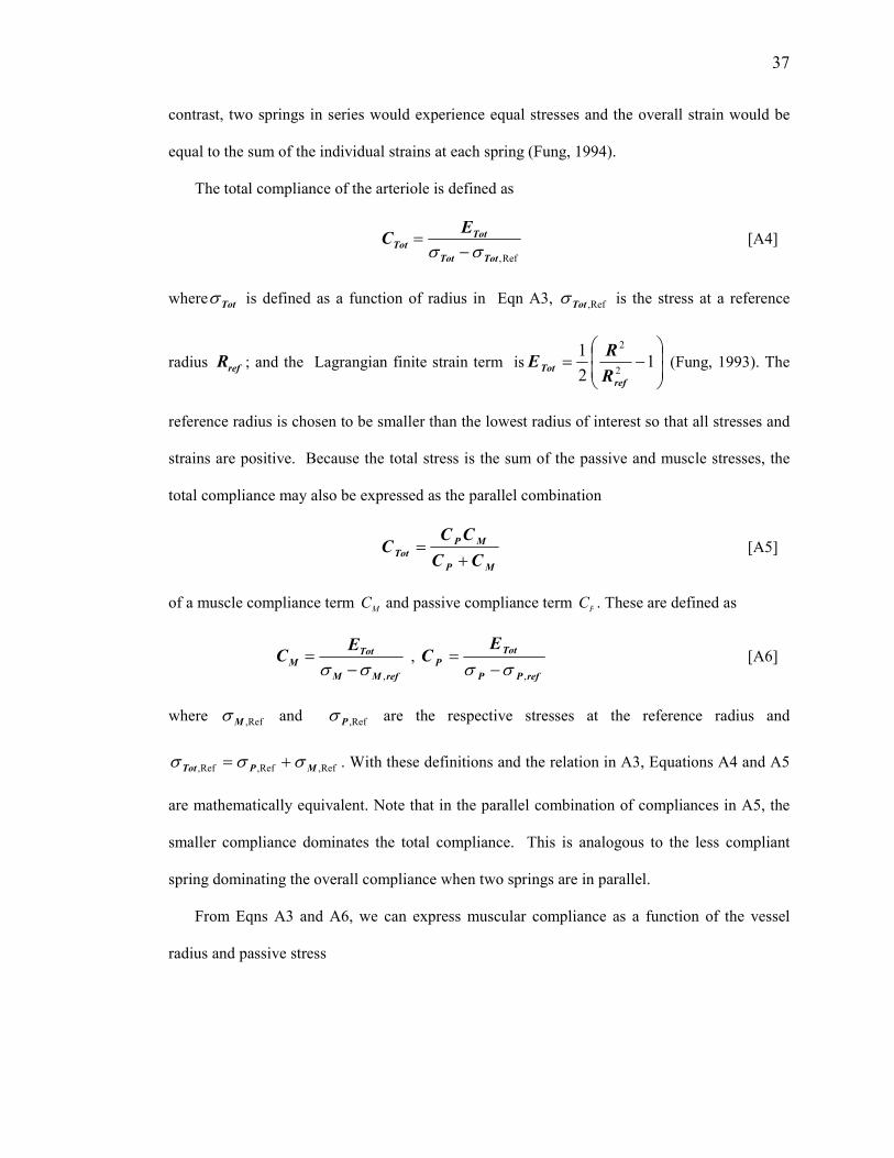
37
contrast, two springs in series would experience equal stresses and the overall strain would be
equal to the sum of the individual strains at each spring (Fung, 1994).
The total compliance of the arteriole is defined as
Ref,TotTot
TotTot
EC
σσ −= [A4]
where Totσ is defined as a function of radius in Eqn A3, Ref,Totσ is the stress at a reference
radius refR ; and the Lagrangian finite strain term is
−= 1
2
12
2
ref
TotR
RE (Fung, 1993). The
reference radius is chosen to be smaller than the lowest radius of interest so that all stresses and
strains are positive. Because the total stress is the sum of the passive and muscle stresses, the
total compliance may also be expressed as the parallel combination
MP
MP
TotCC
CCC
+= [A5]
of a muscle compliance term CM and passive compliance term C
P. These are defined as
refMM
TotM
EC
,σσ −= ,
refPP
Tot
P
EC
,σσ −= [A6]
where Ref,Mσ and Ref,Pσ are the respective stresses at the reference radius and
Ref,Ref,Ref, MPTot σσσ += . With these definitions and the relation in A3, Equations A4 and A5
are mathematically equivalent. Note that in the parallel combination of compliances in A5, the
smaller compliance dominates the total compliance. This is analogous to the less compliant
spring dominating the overall compliance when two springs are in parallel.
From Eqns A3 and A6, we can express muscular compliance as a function of the vessel
radius and passive stress

38
( )fPP
ref
ref
i
Tot
M
h
R
h
RP
EC
Re,σσ −−
−
= . [A7]
It has been shown that passive stress is well modeled as an exponential function of radius
)exp(0, Rk PPP σσ = [A8]
where 0,Pσ and Pk are empirical constants (Fung, 1997). Estimation of these constants is
based on the following observations: (a) the ratio of the stress in the elastic to the muscle
element as a function of radius is conserved across various orders of the arteriole tree; (b) at the
normal operating point radius nR , 80-90% of the total tension is within the muscle element;
and (c) nearly all the stress is exerted by the passive element when the vessel is at its maximum
radius maxR (Davis et al., 1989; Lash et al., 1991). Application of the boundary conditions at
nR and maxR in conjunction with Eqn A3 for the total stress yields
−
−
=
n
n
RR
RR
n
n
n
niP
hR
hR
h
RP max
max
max
λλ
σ [A9]
where λ is the fraction of total stress in the passive element at nR , and nh and maxh are the
vessel wall thickness at nR and maxR , respectively. Substitution of Eqn A9 into Eqn. A7 yields
an expression for muscular compliance as a function of radius
−
−
−
−
=
−
−
−
−
n
nref
n
n
RR
RR
n
nRR
RR
n
n
n
ni
ref
ref
i
ref
M
hR
hR
hR
hR
h
RP
h
R
h
RP
R
R
C
maxmax
max
max
max
max
2
2
12
1
λλλ
[A10]
Assuming an intravascular pressure of 45 mmHg with a normal operating point radius and wall
thickness of 35 and 7 microns; respectively, we use Equation A10 to plot the relation between

39
radius and muscle compliance in Figure 1c. Additionally, the reference radius was selected to
be half of the resting radius with λ and nRRmax set to 0.15 and 1.3, respectively. This
relation is fairly well approximated by the exponential form ( )mCaeaRR 2
1max 1−−= , also
shown in the Figure 1c.
2.7.2 Balloon Model
In the balloon model with viscoelastic effects, the venous compartment is treated as a
distensible balloon (Buxton et al., 1998). The flow into the balloon is determined by the
compliance model, while the flow out of the balloon is modeled as
vvvf vout&τα +=
1
)( [A11]
where v denotes the venous volume normalized by its initial value, vτ is the viscoelastic time
constant (equal to +τ and −τ during inflation and deflation, respectively), and α is an empirical
constant that determines the steady state power law relation between flow and volume (Buxton
et al., 1998; Grubb et al., 1974). The flow and volume dynamics follow the mass conservation
relation
)(0 vffv out−=&τ [A12]
where 0τ is the mean transit time to traverse the venous compartment at rest.
The equation for mass conservation of deoxyhemoglobin in the balloon is
v
qvf
E
EfEfq out )(
),(
0
00 −=&τ [A13]
where q is the total deoxyhemoglobin content normalized by its initial value, 0E is the net
extraction fraction of oxygen at rest, and ),( 0EfE is the extraction fraction as a function of
flow and 0E . An expression for ),( 0EfE is obtained by assuming a linear coupling

40
1
1
0,22
0
−
−=
∆
∆=
m
f
CMROCMRO
CBFCBFn [A14]
between the fractional change in CBF and the fractional change in CMRO2, where n is an
empirical coupling constant and m is CMRO2 normalized by its initial value (Buxton, 2002).
The relation between CBF and CMRO2 is CBFCECMRO A ⋅⋅=2 where AC is the arterial
oxygen concentration. This may be written in normalized quantities as f
mEE
0= .
Combining this expression with Eqn A14 yields
nf
nfEEfE
1),( 00
−+= [A15]
which permits us to rewrite Eqn A13 as
v
qvf
n
nfq out )(
10 −
−+=&τ [A16]
The BOLD signal change as a function of normalized volume and deoxyhemoglobin is
[ ])1)(()1)((/ 322100 vkkqkkVSS −+−−+=∆ [A17]
where 0V is the resting blood volume fraction (Obata et al., 2004). The first constant term
TEEk 001 3.4 ν= where TE is the echo time of the sequence and -1
00 s )5.1/(3.40 B⋅=ν is a
magnetic field ( 0B ) dependent frequency offset. The second constant term TEErk 002 β=
where IE SS=β is the intrinsic ratio of blood to tissue signals at rest and r0 is the slope of
the intravascular relaxation rate *
,2 IR versus the extraction fraction E (Li et al., 1998). The
blood and tissue signals are defined as )/exp( ,20,
∗−= EEE TTESS and
)/exp( ,20,
∗−= III TTESS , respectively, where *
2 IT and *
2ET are the resting intravascular and
extravascular transverse relaxation times and 0ES and EIS are the effective spin densities. For

41
this paper we assume average values of 25,2 =∗ET ms and 8.12,2 =∗
IT ms at 7 Tesla (Yacoub
et al., 2001) and also assume that the effective spin densities are equal. In vitro measurements
have shown that 0r exhibits a quadratic dependence on field strength (Silvennoinen et al.,
2003), so that we may calculate its value as a function of field strength as
( )200 5.1/0.25 Br ⋅= where -1s 0.25 is the measured in-vivo value at 1.5 T (Li et al., 1998;
Obata et al., 2004). Finally, the third constant term is defined as 13 −= βk .
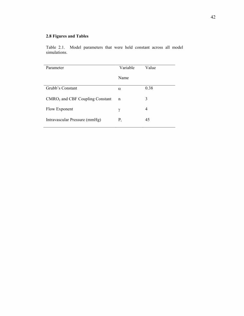
42
2.8 Figures and Tables
Table 2.1. Model parameters that were held constant across all model simulations.
Parameter Variable
Name
Value
Grubb’s Constant α 0.38
CMRO2 and CBF Coupling Constant n 3
Flow Exponent γ 4
Intravascular Pressure (mmHg) Pi 45

43
Table 2.2. Description of model parameters that were adjusted to reflect either carbon dioxide level-related or age-related changes in the normalized baseline
cerebral blood flow YNCBFCBFf ,000 = where YNCBF ,0 denotes baseline CBF
for normocapnia in the young state. Initial radius is γ/1
0,00 fRR YN= where YNR ,0
is the initial radius for the young normocapnic state and 4=γ for laminar flow.
The initial wall thicknesses 0h for the hypocapnic and hypercapnic states were
computed using the incompressibility constraint in Eq A2, whereas the initial wall
thickness for the old state was assumed to be 20% of 0R . The passive stress
fraction λ at rest is used to generate the stress versus radius operating curves for
the young and old states. It therefore corresponds to the stress fraction for the normocapnic condition in either the young or old state. Initial muscular compliance
0,MC and total compliance 0,TOTC for each state were calculated from Equations
A5 and A10 with appropriate substitutions. The resting venous volume fraction 0V
was determined for each state with a Grubb’s law relation α00 )025.0( fV = . With
the assumption of no change in baseline CMRO2 between carbon dioxide levels, the
resting oxygen fraction 0E for each state is 0,00 fEE YN= where YNE ,0 denotes
the young normocapnic value. Reflecting the assumed decrease in CMRO2 with age, the extraction fraction for the aged state is equal to that for the young
normocapnic state. The resting transit delay 0τ in each state reflects the central
volume principle 000 /CBFV=τ .
Parameter Normocapnia/
Young
Hypocapnia Hypercapnia Old
CBF0 /CBF0,YN 1.0 0.8 1.3 0.8
0R (µm) 35.0 33.1 37.4 33.1
h0 (µm) 7.0 7.33 6.62 6.62
λ 0.15 0.15 0.15 0.25
CM ,0 (1/mmHg) 0.012 0.011 0.014 0.013
CTOT ,0(1/mmHg) 0.00956 0.00954 0.00958 0.00856
0V 0.025 0.023 0.028 0.023
0E 0.4 0.5 0.31 0.4
0τ (s) 2.5 2.87 2.13 2.87
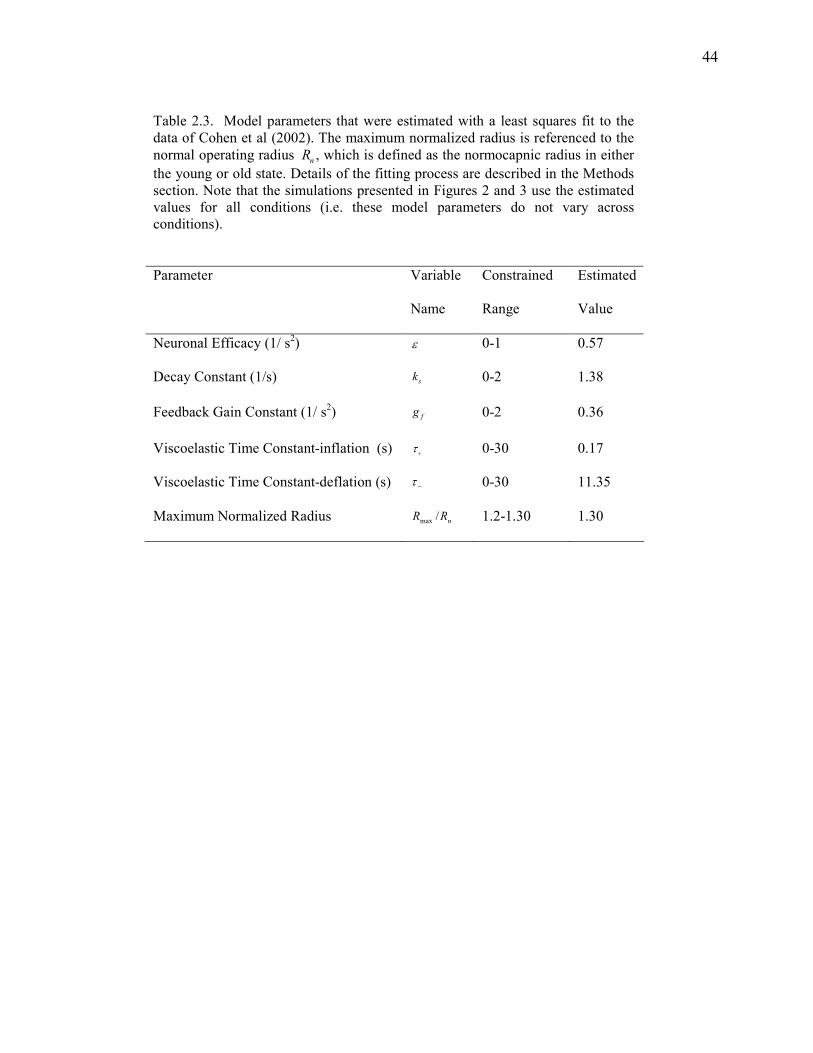
44
Table 2.3. Model parameters that were estimated with a least squares fit to the data of Cohen et al (2002). The maximum normalized radius is referenced to the
normal operating radius Rn, which is defined as the normocapnic radius in either
the young or old state. Details of the fitting process are described in the Methods section. Note that the simulations presented in Figures 2 and 3 use the estimated values for all conditions (i.e. these model parameters do not vary across conditions).
Parameter Variable
Name
Constrained
Range
Estimated
Value
Neuronal Efficacy (1/ s2) ε 0-1 0.57
Decay Constant (1/s) sk 0-2 1.38
Feedback Gain Constant (1/ s2) fg 0-2 0.36
Viscoelastic Time Constant-inflation (s) τ+ 0-30 0.17
Viscoelastic Time Constant-deflation (s) −τ 0-30 11.35
Maximum Normalized Radius Rmax /Rn 1.2-1.30 1.30
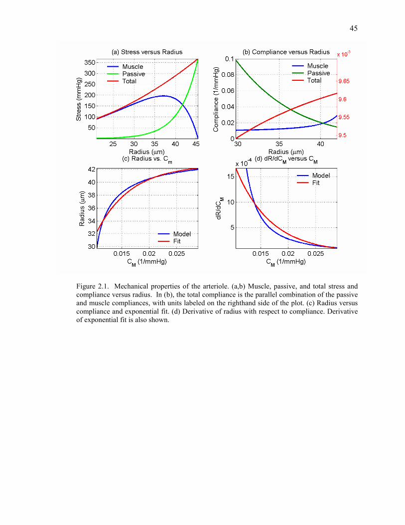
45
Figure 2.1. Mechanical properties of the arteriole. (a,b) Muscle, passive, and total stress and compliance versus radius. In (b), the total compliance is the parallel combination of the passive and muscle compliances, with units labeled on the righthand side of the plot. (c) Radius versus compliance and exponential fit. (d) Derivative of radius with respect to compliance. Derivative of exponential fit is also shown.

46
Figure 2.2. Model responses under hypocapnic, normocapnic, and hypercapnic conditions. Data from (Cohen et al., 2002) are shown by the plus symbols in panel (d)

47
Figure 2.3. (a) Stress versus radius for young and old subject. (b) dR/dCM versus normalized radius (c,d) Model CBF and BOLD responses.
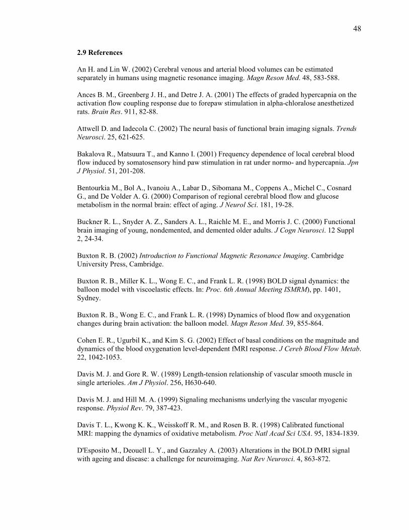
48
2.9 References
An H. and Lin W. (2002) Cerebral venous and arterial blood volumes can be estimated separately in humans using magnetic resonance imaging. Magn Reson Med. 48, 583-588. Ances B. M., Greenberg J. H., and Detre J. A. (2001) The effects of graded hypercapnia on the activation flow coupling response due to forepaw stimulation in alpha-chloralose anesthetized rats. Brain Res. 911, 82-88. Attwell D. and Iadecola C. (2002) The neural basis of functional brain imaging signals. Trends Neurosci. 25, 621-625. Bakalova R., Matsuura T., and Kanno I. (2001) Frequency dependence of local cerebral blood flow induced by somatosensory hind paw stimulation in rat under normo- and hypercapnia. Jpn J Physiol. 51, 201-208. Bentourkia M., Bol A., Ivanoiu A., Labar D., Sibomana M., Coppens A., Michel C., Cosnard G., and De Volder A. G. (2000) Comparison of regional cerebral blood flow and glucose metabolism in the normal brain: effect of aging. J Neurol Sci. 181, 19-28. Buckner R. L., Snyder A. Z., Sanders A. L., Raichle M. E., and Morris J. C. (2000) Functional brain imaging of young, nondemented, and demented older adults. J Cogn Neurosci. 12 Suppl 2, 24-34. Buxton R. B. (2002) Introduction to Functional Magnetic Resonance Imaging. Cambridge University Press, Cambridge. Buxton R. B., Miller K. L., Wong E. C., and Frank L. R. (1998) BOLD signal dynamics: the balloon model with viscoelastic effects. In: Proc. 6th Annual Meeting ISMRM), pp. 1401, Sydney. Buxton R. B., Wong E. C., and Frank L. R. (1998) Dynamics of blood flow and oxygenation changes during brain activation: the balloon model. Magn Reson Med. 39, 855-864. Cohen E. R., Ugurbil K., and Kim S. G. (2002) Effect of basal conditions on the magnitude and dynamics of the blood oxygenation level-dependent fMRI response. J Cereb Blood Flow Metab. 22, 1042-1053. Davis M. J. and Gore R. W. (1989) Length-tension relationship of vascular smooth muscle in single arterioles. Am J Physiol. 256, H630-640. Davis M. J. and Hill M. A. (1999) Signaling mechanisms underlying the vascular myogenic response. Physiol Rev. 79, 387-423. Davis T. L., Kwong K. K., Weisskoff R. M., and Rosen B. R. (1998) Calibrated functional MRI: mapping the dynamics of oxidative metabolism. Proc Natl Acad Sci USA. 95, 1834-1839. D'Esposito M., Deouell L. Y., and Gazzaley A. (2003) Alterations in the BOLD fMRI signal with ageing and disease: a challenge for neuroimaging. Nat Rev Neurosci. 4, 863-872.

49
D'Esposito M., Zarahn E., Aguirre G. K., and Rypma B. (1999) The effect of normal aging on the coupling of neural activity to the BOLD hemodynamic response. NeuroImage. 10, 6-14. Friston K. J. (2002) Bayesian estimation of dynamical systems: an application to fMRI. Neuroimage. 16, 513-530. Friston K. J., Harrison L., and Penny W. (2003) Dynamic causal modelling. Neuroimage. 19, 1273-1302. Friston K. J., Mechelli A., Turner R., and Price C. J. (2000) Nonlinear Responses in fMRI: The Balloon Model, Volterra Kernels, and Other Hemodynamics. NeuroImage. 12, 466-477. Fung Y. (1993) Biomechanics: Mechanical Properties of Living Tissues. Springer-Verlag, New York. Fung Y. (1994) A First Course in Continuum Mechanics, Third edn. Prentice Hall, New Jersey. Fung Y. C. (1997) Biomechanics: Circulation. Springer-Verlag, New York. Grubb R. L., Raichle M. E., Eichling J. O., and Ter-Pogossian M. M. (1974) The effects of changes in PaCO2 on cerebral blood volume, blood flow, and vascular mean transit time. Stroke. 5, 630 - 639. Hajdu M. A., Heistad D. D., Siems J. E., and Baumbach G. L. (1990) Effects of aging on mechanics and composition of cerebral arterioles in rats. Circ Res. 66, 1747-1754. Handwerker D. A., Ollinger J. M., and D'Esposito M. (2004) Variation of BOLD hemodynamic responses across subjects and brain regions and their effects on statistical analyses. Neuroimage. 21, 1639-1651. Hoge R. D., Atkinson J., Gill B., Crelier G. R., Marrett S., and Pike G. B. (1999) Linear coupling between cerebral blood flow and oxygen consumption in activated human cortex. Proc Natl Acad Sci U S A. 96, 9403-9408. Iadecola C. (2004) Neurovascular regulation in the normal brain and in Alzheimer's disease. Nat Rev Neurosci. 5, 347-360. Irikura K., Maynard K. I., and Moskowitz M. A. (1994) Importance of nitric oxide synthase inhibition to the attenuated vascular responses induced by topical L-nitroarginine during vibrissal stimulation. J Cereb Blood Flow Metab. 14, 45-48. Ito H., Kanno I., Ibaraki M., Hatazawa J., and Miura S. (2003) Changes in human cerebral blood flow and cerebral blood volume during hypercapnia and hypocapnia measured by positron emission tomography. J Cereb Blood Flow Metab. 23, 665-670. Kashikura K., Kershaw J., Kashikura A., Zhang X., Matsuura T., and Kanno I. (2001) Hyperoxia modified activation-induced blood oxygenation level-dependent response of human

50
visual cortex (V1): an event-related functional magnetic resonance imaging study. Neurosci Lett. 299, 53-56. Kastrup A., Kruger G., Neumann-Haefelin T., Glover G. H., and Moseley M. E. (2002) Changes of cerebral blood flow, oxygenation, and oxidative metabolism during graded motor activation. Neuroimage. 15, 74-82. Kemna L. J. and Posse S. (2001) Effect of respiratory CO(2) changes on the temporal dynamics of the hemodynamic response in functional MR imaging. Neuroimage. 14, 642-649. Lash J. M., Bohlen H. G., and Waite L. (1991) Mechanical characteristics and active tension generation in rat intestinal arterioles. Am J Physiol. 260, H1561-1574. Leenders K. L., Perani D., Lammertsma A. A., Heather J. D., Buckingham P., Healy M. J. R., Gibbs J. M., Wise R. J. S., Hatazawa J., Herold S., Beaney R. P., Brooks D. B., Spinks T., Rhodes C., Frackowiak R. S. J., and Jones T. (1990) Cerebral blood flow, blood volume and oxygen utilization: Normal values and effect of age. Brain. 113, 27-47. Li D., Wang Y., and Waight D. J. (1998) Blood oxygen saturation assessment in vivo using T2* estimation. Magn Reson Med. 39, 685-690. Logothetis N. K. and Wandell B. A. (2004) Interpreting the BOLD signal. Annu Rev Physiol. 66, 735-769. Mandeville J. B., Marota J. J. A., Ayata C., Zaharchuk G., Moskowitz M. A., Rosen B. R., and Weisskoff R. M. (1999) Evidence of a cerebrovascular postarteriole windkessel with delayed compliance. J Cereb Blood Flow Metab. 19, 679-689. Marchal G., Rioux P., Petit-Taboue M.-C., Sette G., Travere J.-M., LePoec C., Courtheoux P., Derlon J.-M., and Baron J.-C. (1992) Regional cerebral oxygen consumption, blood flow, and blood volume in healthy human aging. Arch Neurol. 49, 1013-1020. Martin A. J., Friston K. J., Colebatch J. G., and Frackowiak R. S. (1991) Decreases in regional cerebral blood flow with normal aging. J Cereb Blood Flow Metab. 11, 684-689. Martinez-Lemus L. A., Wu X., Wilson E., Hill M. A., Davis G. E., Davis M. J., and Meininger G. A. (2003) Integrins as unique receptors for vascular control. J Vasc Res. 40, 211-233. Matsuura T., Fujita H., Kashikura K., and Kanno I. (2000) Evoked local cerebral blood flow induced by somatosensory stimulation is proportional to the baseline flow. Neurosci Res. 38, 341-348. Matsuura T., Fujita H., Kashikura K., and Kanno I. (2000) Modulation of evoked cerebral blood flow under excessive blood supply and hyperoxic conditions. Jpn J Physiol. 50, 115-123. Matsuura T., Kashikura K., and Kanno I. (2001) Hemodynamics of local cerebral blood flow induced by somatosensory stimulation under normoxia and hyperoxia in rats. Comp Biochem Physiol A Mol Integr Physiol. 129, 363-372.

51
Mayhew J. E., Askew S., Zheng Y., Porrill J., Westby G. W., Redgrave P., Rector D. M., and Harper R. M. (1996) Cerebral vasomotion: a 0.1-Hz oscillation in reflected light imaging of neural activity. Neuroimage. 4, 183-193. Mehagnoul-Schipper D. J., van der Kallen B. F., Colier W. N., van der Sluijs M. C., van Erning L. J., Thijssen H. O., Oeseburg B., Hoefnagels W. H., and Jansen R. W. (2002) Simultaneous measurements of cerebral oxygenation changes during brain activation by near-infrared spectroscopy and functional magnetic resonance imaging in healthy young and elderly subjects. Hum Brain Mapp. 16, 14-23. Mildner T., Norris D. G., Schwarzbauer C., and Wiggins C. J. (2001) A Qualitative Test of the Balloon Model for BOLD-based MR Signal Changes at 3T. Magn Reson Med. 46, 891-899. Miller K. L., Luh W. M., Liu T. T., Martinez A., Obata T., Wong E. C., Frank L. R., and Buxton R. B. (2001) Nonlinear temporal dynamics of the cerebral blood flow response. Hum Brain Mapp. 13, 1-12. Murray K. J. (1990) Cyclic AMP and mechanisms of vasodilation. Pharmacol Ther. 47, 329-345. Obata T., Liu T. T., Miller K. L., Luh W. M., Wong E. C., Frank L. R., and Buxton R. B. (2004) Discrepancies between BOLD and flow dynamics in primary and supplementary motor areas: application of the balloon model to the interpretation of BOLD transients. Neuroimage. 21, 144-153. Panczel G., Daffertshofer M., Ries S., Spiegel D., and Hennerici M. (1999) Age and stimulus dependency of visually evoked cerebral blood flow responses. Stroke. 30, 619-623. Pantano P., Baron J. C., Lebrun-Grandie P., Duquesnoy N., Bousser M. G., and Comar D. (1984) Regional cerebral blood flow and oxygen consumption in human aging. Stroke. 15, 635-641. Richter W. and Richter M. (2003) The shape of the fMRI BOLD response in children and adults changes systematically with age. Neuroimage. 20, 1122-1131. Riddle D. R., Sonntag W. E., and Lichtenwalner R. J. (2003) Microvascular plasticity in aging. Ageing Res Rev. 2, 149-168. Rosengarten B., Spiller A., Aldinger C., and Kaps M. (2003) Control system analysis of visually evoked blood flow regulation in humans under normocapnia and hypercapnia. Eur J Ultrasound. 16, 169-175. Rostrup E., Law I., Pott F., Ide K., and Knudsen G. M. (2002) Cerebral hemodynamics measured with simultaneous PET and near-infrared spectroscopy in humans. Brain Res. 954, 183-193. Schroeter M. L., Zysset S., Kruggel F., and von Cramon D. Y. (2003) Age dependency of the hemodynamic response as measured by functional near-infrared spectroscopy. Neuroimage. 19, 555-564.

52
Silva A. C., Iadecola C., and Kim S.-G. (1999) The Dependence of BOLD and CBF Changes on the CBF Baseline during Somatsensory Simulation. In: Seventh ISMRM Scientific Meeting), pp. 1736, Philadelphia, PA. Silvennoinen M. J., Clingman C. S., Golay X., Kauppinen R. A., and van Zijl P. C. (2003) Comparison of the dependence of blood R2 and R2* on oxygen saturation at 1.5 and 4.7 Tesla. Magn Reson Med. 49, 47-60. Somlyo A. P. and Somlyo A. V. (1994) Signal transduction and regulation in smooth muscle. Nature. 372, 231-236. Stewart G. N. (1894) Researches on the circulation time in organs and on the influences which affect it. J Physiol (London). 15, Parts I-III. Taoka T., Iwasaki S., Uchida H., Fukusumi A., Nakagawa H., Kichikawa K., Takayama K., Yoshioka T., Takewa M., and Ohishi H. (1998) Age correlation of the time lag in signal change on EPI-fMRI. J Comput Assist Tomogr. 22, 514-517. Ursino M. (1991) Mechanisms of cerebral blood flow regulation. Critical Reviews in Biomedical Engineering. 18, 255-288. West G. A., Meno J. R., Nguyen T. S., Ngai A. C., Simard J. M., and Winn H. R. (2003) cGMP-dependent and not cAMP-dependent kinase is required for adenosine-induced dilation of intracerebral arterioles. J Cardiovasc Pharmacol. 41, 444-451. Wilson H. R. (1999) Spikes, Decisions and Actions: Dynamical Foundations of Neuroscience. Oxford University Press, Oxford. Yacoub E., Shmuel A., Pfeuffer J., Van De Moortele P. F., Adriany G., Andersen P., Vaughan J. T., Merkle H., Ugurbil K., and Hu X. (2001) Imaging brain function in humans at 7 Tesla. Magn Reson Med. 45, 588-594. Yang J., Clark J. W., Jr., Bryan R. M., and Robertson C. (2003) The myogenic response in isolated rat cerebrovascular arteries: smooth muscle cell model. Med Eng Phys. 25, 691-709. Yang J., Clark J. W., Jr., Bryan R. M., and Robertson C. S. (2003) The myogenic response in isolated rat cerebrovascular arteries: vessel model. Med Eng Phys. 25, 711-717. Zheng Y., Martindale J., Johnston D., Jones M., Berwick J., and Mayhew J. (2002) A model of the hemodynamic response and oxygen delivery to brain. Neuroimage. 16, 617-637.

53
Chapter 3
Caffeine Reduces the Initial Dip in the Visual BOLD
Response at 3T
3.1 Abstract
Localized changes in oxygen consumption related to increased neural activity can result in a
small and transient “initial dip” of the blood oxygenation level-dependent (BOLD) signal used
in functional magnetic resonance imaging (fMRI). The initial dip has been of great interest to
the fMRI community because it may provide a more accurate and localized measure of neural
activity than the conventional BOLD signal increase. Although potentially useful as a
technique for human brain mapping, the initial dip is not always detected and has been a source
of some controversy. In this study, the BOLD response to a 4-s long visual stimulus was
measured with a 3 Tesla MRI system in 5 healthy volunteers both before and immediately after
a 200-mg oral caffeine dose. The caffeine dose significantly (P < 0.001) reduced or eliminated
the initial dip in all subjects. These findings suggest that caffeine usage may be a key factor in
the detection of the initial dip in human fMRI studies.
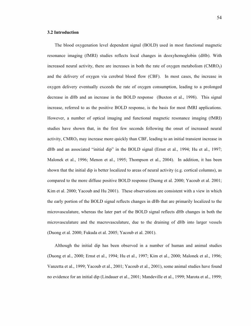
54
3.2 Introduction
The blood oxygenation level dependent signal (BOLD) used in most functional magnetic
resonance imaging (fMRI) studies reflects local changes in deoxyhemoglobin (dHb). With
increased neural activity, there are increases in both the rate of oxygen metabolism (CMRO2)
and the delivery of oxygen via cerebral blood flow (CBF). In most cases, the increase in
oxygen delivery eventually exceeds the rate of oxygen consumption, leading to a prolonged
decrease in dHb and an increase in the BOLD response (Buxton et al., 1998). This signal
increase, referred to as the positive BOLD response, is the basis for most fMRI applications.
However, a number of optical imaging and functional magnetic resonance imaging (fMRI)
studies have shown that, in the first few seconds following the onset of increased neural
activity, CMRO2 may increase more quickly than CBF, leading to an initial transient increase in
dHb and an associated “initial dip” in the BOLD signal (Ernst et al., 1994; Hu et al., 1997;
Malonek et al., 1996; Menon et al., 1995; Thompson et al., 2004). In addition, it has been
shown that the initial dip is better localized to areas of neural activity (e.g. cortical columns), as
compared to the more diffuse positive BOLD response (Duong et al. 2000; Yacoub et al. 2001;
Kim et al. 2000; Yacoub and Hu 2001). These observations are consistent with a view in which
the early portion of the BOLD signal reflects changes in dHb that are primarily localized to the
microvasculature, whereas the later part of the BOLD signal reflects dHb changes in both the
microvasculature and the macrovasculature, due to the draining of dHb into larger vessels
(Duong et al. 2000; Fukuda et al. 2005; Yacoub et al. 2001).
Although the initial dip has been observed in a number of human and animal studies
(Duong et al., 2000; Ernst et al., 1994; Hu et al., 1997; Kim et al., 2000; Malonek et al., 1996;
Vanzetta et al., 1999; Yacoub et al., 2001; Yacoub et al., 2001), some animal studies have found
no evidence for an initial dip (Lindauer et al., 2001; Mandeville et al., 1999; Marota et al., 1999;

55
Silva et al., 2000). It has been suggested that differences in imaging methodology, brain
regions, animal species, and anesthesia are responsible for the conflicting observations in
animal studies (Ances, 2004; Buxton, 2001). One human fMRI study suggested that the initial
dip may be an experimental artifact that arises when stimuli are too closely spaced in time
(Fransson et al., 1998), but a subsequent study found an initial dip even with wider spacings
(Yacoub et al., 1999). While there do not appear to be additional human fMRI studies that
explicitly focus on the absence of the initial dip, there are many studies of the dynamics of the
BOLD response that either do not find or simply do not mention the initial dip. For example,
the initial dip was not observed in studies examining the effects of carbon dioxide on the BOLD
response (Cohen et al., 2002; Kemna et al., 2001). Cohen et al attributed the lack of detection
to differences in experimental methodology, which can be an important factor given the
relatively small amplitude of the initial dip.
In addition to methodological differences, variations in the baseline vascular state due to
factors such as pharmacological agents, disease, and age have been shown to alter the dynamics
of the BOLD response and may therefore affect the detection of the initial dip in humans
(D'Esposito et al., 2003). As an example, the carbon dioxide studies mentioned above found
that vasodilation caused by hypercapnia significantly slowed down the dynamics of the BOLD
response, while vasoconstriction caused by hypocapnia led to a quickening of the response. In a
recent study using a 4 Tesla MRI system, we showed that caffeine, a known vasoconstrictor, led
to a quickening of the visual BOLD response in a manner similar to that observed with
hypocapnia (Liu et al., 2004). Due to technical considerations (e.g. scanner instabilities), the
initial dip was not easily detected in that study. In the present study, performed on a 3 Tesla
MRI system, we demonstrate robust detection of the initial dip and show that a 200 mg caffeine
dose can significantly reduce the initial dip.

56
3.3 Methods
3.3.1 Experimental Protocol
Five healthy subjects (ages 23 to 39) participated in the study after giving informed consent.
Each subject refrained from ingesting any food or drink containing caffeine for at least 12 hours
prior to the experiment. The estimated daily caffeine usage of the subjects based on self-reports
of coffee, tea, and caffeinated soda consumption is summarized in Table 1. The assumed
caffeine contents for an 8-oz coffee, tea, and soda were 100 mg, 40 mg, and 20 mg, respectively
(Fredholm et al., 1999). Each experiment lasted approximately 3 hours and consisted of a 1-
hour pre-dose imaging session followed by a 1-hour post-dose session. In addition to the actual
time spent on imaging, the length of each session included time for preparation (e.g. ensuring
that physiological monitoring equipment was working properly), parameter set-up and
execution of prescan routines (as necessary), and instruction of the subject prior to each scan.
Between sessions the subject ingested an over-the-counter tablet containing 200-mg of caffeine
and rested outside the scanner for approximately 30 minutes. The first functional run began
approximately 45 minutes post ingestion. This interval was chosen based on studies showing
that the absorption of caffeine from the gastrointestinal tract reaches 99% about 45 minutes after
ingestion, with a half-life of 2.5 to 4.5 hours (Fredholm et al., 1999).
During both the pre-dose and post-dose imaging sessions, each subject viewed two repeats
of a periodic single trial visual stimulus consisting of a 20-second initial “off” period followed
by 5 cycles of a 4 second “on” period and a 40 second “off” period. During the “on” periods, a
full-field, full contrast radial 8 Hz flickering checkerboard was displayed, while the “off”
periods consisted of a gray background of luminance equal to the average luminance of the “on”
period. Three of the five subjects viewed two additional repeats of the periodic single trial
design. As described below, these were acquired with a smaller imaging slice thickness than

57
the first two repeats. In addition, a resting-state scan, during which the subject was presented
with the “off” condition for 3 minutes, was performed and used to characterize the resting CBF
level.
3.3.2 Imaging Protocol
Imaging data were collected on a GE Signa Excite 3 Tesla whole body system with a body
transmit coil and an eight channel receive coil. Laser alignment was used to landmark the
subject and minimize differences in head position between sessions. During the resting-state
scan, data were acquired with a PICORE QUIPPS II (Wong et al., 1998) arterial spin labeling
(ASL) sequence (TR= 2s , TI1/TI2= 600/1500ms, 10 cm tag thickness, and a 1 cm tag-slice
gap) with a dual echo spiral readout (TE1/TE2=9.1/30 ms, FOV=24 cm, 64x64 matrix, and a
flip angle= 90 degrees). Small bipolar crusher gradients were included to remove signal from
large vessels (b=2 s/mm2). Three oblique axial 8 mm slices were prescribed about the calcarine
sulcus for this ASL run. During the periodic single trial runs, BOLD-weighted images were
acquired with a spiral readout (TE=25ms, TR=500 ms, FOV=24cm, 64x64 matrix, and a flip-
angle of 45 degrees). In all five subjects, these BOLD runs used the same slice prescription as
the ASL runs (e.g. three 8 mm slices). The choice of the 8mm slice thickness reflects the fact
that the experiments on two of the subjects (labeled as Subjects 4 and 5 in Results) were not
originally intended to examine the initial dip. To determine whether there was an effect of the
large slice thickness, the experiments in the three remaining subjects (labeled 1 to 3 in Results)
included two additional BOLD-weighted runs using the periodic single trial design and acquired
with six oblique 4 mm slices covering the same volume as the three 8 mm slices. For all
periodic single trials acquired at either slice thickness, 480 volumes at a TR of 500 ms were
acquired.

58
A high resolution structural scan was acquired with a magnetization prepared 3D fast
spoiled gradient acquisition in the steady state (FSPGR) sequence (TI 450ms, TR 7.9ms, TE
3.1ms, 12 degree flip angle, FOV 25x25x16 cm, matrix 256x256x124). In addition, a
cerebrospinal fluid (CSF) reference scan and a minimum contrast scan were acquired for use in
CBF quantification. The CSF scan consisted of a single-echo, single repetition scan acquired at
full relaxation and echo time equal to 9.1 ms, while the minimal contrast scan was acquired at
TR=2 sec and TE=11 ms. Both scans used the same in-plane parameters as the ASL scans, but
the number of slices was increased to cover the lateral ventricles.
Cardiac pulse and respiratory effort data were monitored using a pulse oximeter (InVivo)
and a respiratory effort transducer (BIOPAC), respectively. The pulse oximeter was placed on
the subject's right index finger, and the respiratory effort belt was placed around the subject's
abdomen. Physiological data were sampled at 40 samples per second using a multi-channel
data acquisition board (National Instruments).
3.3.3 Data Analysis
All images were coregistered using AFNI software (Cox, 1996). The structural scan from
each post-dose session was aligned to the structural scan of its respective pre-dose session, and
the rotation and shift matrix used for this alignment was then applied to the post-dose BOLD
and ASL images. An image-based retrospective correction method RETROICOR (Glover et
al., 2000; Restom et al., 2004) was used to reduce physiological noise due to cardiac and
respiratory fluctuations. For each subject, a mean ASL image was formed from the average
difference of the control and tag images from the resting-state scan data. This mean ASL image
was then corrected for coil inhomogeneities using the minimum contrast image (Wang et al.,
2005) and converted to physiological units using the CSF image as a reference signal (Chalela
et al., 2000).

59
For each slice thickness, average BOLD time series were formed from the data (after
physiological noise correction) for the two runs acquired at that thickness. All subsequent
analyses were performed separately for the average BOLD time series. Correlation analysis was
performed using a positive BOLD reference function formed by convolving the periodic single
trial stimulus pattern with a gamma density function of the form
h(t) = (τn!)−1 t −∆t( )/τ( )n exp − t −∆t( )/τ( ) for t ≥ ∆t and 0 otherwise, with τ = 1.2, n = 3
and ∆t =1. A constant term and linear trend term were used as nuisance terms in the correlation
analysis.
Functional regions of interest (ROI) were defined for the pre-dose (ROIpre) and post-dose
(ROIpost) data using a correlation coefficient threshold of 0.40 based on the positive BOLD
response. A joint functional ROI (ROIjoint) was then formed from the intersection of ROIpre
and ROIpost, using a spatial clustering criterion (one nearest neighbor) to eliminate isolated
voxels. The area of the first 2.5 seconds of the average BOLD response, referred to as the initial
dip area, was computed for each voxel within ROIjoint, with a negative area corresponding to the
presence of an initial dip. Voxels within ROIjoint displaying an initial dip in the pre-dose data
were then used to define an initial dip ROI, denoted as ROIdip. In other words, ROIdip
encompasses all voxels in ROIjoint that display an initial dip in the pre-dose periodic BOLD
response.
Note that for subjects with both 4 mm and 8 mm slice thickness data, a separate ROIdip was
defined for each slice thickness. For each voxel within ROIdip the average BOLD response was
formed by averaging across cycles of the average BOLD time series. For each subject, a mean
BOLD response was then computed for ROIdip and a paired t-test (two-tailed) was used to
compare the pre-dose and post-dose initial dip areas across all voxels within ROIdip. In
addition, the average CBF was computed for ROIdip, and a paired t-test (two-tailed) was used to
compare the pre-dose and post-dose CBF levels across voxels in ROIdip .

60
An additional correlation analysis was performed to show localization of the initial dip, but
was not used for further statistical comparisons. The initial dip reference function was a
symmetric triangle that started at 0.5 seconds, peaked at 1.5 seconds with a negative amplitude
of -0.5, and returned to zero at 2.5 seconds (total duration = 2 seconds). A spatial clustering
criterion (one nearest neighbor) was used to eliminate isolated voxels.
3.4 Results
The group average pre-dose (blue) and post-dose (red) BOLD responses (N = 5) from the
8mm slice thickness data are shown in the top row of Figure 1, with panel (b) depicting a
magnified view of the initial response. Consistent with prior findings (Liu et al., 2004), the
administration of caffeine speeds up the BOLD response with a decrease in peak-time from 8.45
s to 7.45 s and full-width half maximum from 6.95 s to 6.1 s. The peak amplitude increased
from 1.83% to 2.16% following caffeine ingestion. In the initial portion of the pre-dose
response, the response dips after the onset of the visual stimulus, reaching a minimum value of
–0.16% at 1.5 seconds, at which time the response begins to recover and becomes positive at 2.5
seconds. In contrast to the pre-dose initial response, the post-dose response increases after the
onset of stimulus. Group average responses from the 4mm slice thickness data (N = 3 subjects)
are shown in the bottom row of Figure 1. The results are similar to those observed for the 8 mm
slice thickness data, with the initial dip clearly visible in the pre-dose response and reduced in
the post-dose response. Following the initial onset of visual stimulation, the pre-dose response
dips to a minimum value of –0.24% at 1.5 s before becoming positive at 2.5 s.
Figure 2 shows the post-dose (y-axis) versus pre-dose (x-axis) initial dip areas from the
ROIdip for each subject. Panels a-c and d-h correspond to the data acquired at 4mm and 8mm
slice thicknesses, respectively. A significant (p < 8.4e-4) reduction of the initial dip (e.g. more
positive initial dip area) was observed for each subject. Figure 3 shows magnified views of the

61
pre-dose (blue) and post-dose (red) average initial responses for each subject. Panels a-c show
the responses from the 4mm slice thickness data while panels d-h are for the 8mm slice
thickness data. The reduction of the initial dip by caffeine is clearly present in each subject’s
responses.
Figure 4 compares the pre-dose and post-dose spatial localization of the initial dip and the
positive BOLD response for a representative slice (4mm thick) from subject 1. Panels a) and
c) show the spatial extent of the initial dip in the pre-dose and post-dose conditions,
respectively, with the colorbar indicating the scale of the correlation coefficient calculated with
the initial dip reference function. Consistent with the above observations of a significant
reduction of the initial dip with caffeine, the spatial extent of the initial dip is greatly diminished
in the post-dose map. Panels b) and d) are positive BOLD activation maps for the pre-dose and
post-dose conditions, respectively, with the colorbar indicating the scale of the correlation
coefficients obtained with the positive BOLD reference function. In comparison to the initial
dip spatial maps the positive BOLD maps exhibit a wider spread of activation across the
occipital cortex, consistent with the findings of prior studies (Yacoub and Hu 2001 and Yacoub
et al. 2001). Spatial localization maps from the other subjects showed similar behavior.
Table 1 shows the average pre-dose and post-dose CBF values for each subject, along with
p-values obtained with two-tailed paired t-tests. The mean and standard deviations of the CBF
were computed using voxels within each subject’s ROIdip. For each subject, there is a
significant reduction (p < 1.7e-11) in CBF associated with the caffeine dose, with the percent
decrease in CBF ranging from 30 to 51% across subjects.
3.5 Discussion
A significant reduction in the initial dip amplitude due to caffeine was observed in each
subject that was studied. This reduction was observed in both 8 mm slice thickness data (N=5)

62
and the 4mm slice thickness data (N=3), indicating that the effect is fairly robust with respect to
voxel size. Consistent with prior studies, the caffeine dose also significantly reduced the
baseline CBF level in each subject (Cameron et al., 1990; Field et al., 2003; Liu et al., 2004).
Why does caffeine reduce the initial dip? Caffeine exerts both neural and vascular effects
through its binding to adenosine receptors in the brain (Fredholm et al., 1999). In particular, its
neurostimulant effects are thought to arise from the inhibition of adenosine A1 receptors, while
its vasoconstrictive effects are believed to be due primarily to the inhibition of adenosine A2A
receptors (Ngai et al., 2001 ). It is reasonable to conjecture that the enhancement of neural
activity with caffeine would primarily affect the CMRO2 response, while vasoconstriction due
to caffeine is more likely to alter the CBF response. The presence of an initial dip is generally
thought to reflect a temporal mismatch between CMRO2 and CBF, with CMRO2 increasingly
more rapidly than CBF following the onset of stimulus (Ances, 2004; Buxton, 2001). A
reduction in the initial dip could therefore reflect either a relative quickening of the CBF
response or a relative slowing down of the CMRO2 response. Given its neurostimulant
properties, it seems unlikely that caffeine would cause the CMRO2 response to become slower.
In contrast, a quickening of the CBF response due to vasoconstriction would be consistent with
the findings of a recent theoretical model introduced by our group (Behzadi et al., 2005).
In the theoretical model, the dynamics of the CBF response depend on the biomechanical
responsiveness of the arterioles, which in turn depends on the relative contributions of the
vascular smooth muscle and connective tissue to the dynamics of the arteriolar wall. With
vasodilatory agents, such as carbon dioxide, the vascular smooth muscle relaxes and exerts less
force so that the arteriole may expand, while the connective tissue becomes stiffer and exerts
more force, similar to the walls of a rubber tube becoming less compliant as it expands. This
makes the arteriole relatively less responsive and slows down the dynamic CBF response. In
contrast, with the application of a vasoconstrictive agent, such as caffeine, the vascular smooth

63
muscle exerts more force in order to constrict the arteriole, while the force exerted by the
connective tissue is reduced. This redistribution of forces makes the arteriole more responsive
and speeds up the dynamic CBF response.
While the above arguments suggest that the reduction in the initial dip is due primarily to a
quickening of the CBF response, an effect of caffeine on the CMRO2 response cannot be ruled
out. It is likely, however, that caffeine-induced changes in the CMRO2 response are smaller
than changes in the CBF response. Further experimental studies directly examining the effect
of caffeine on the CBF and CMRO2 responses would be useful for clarifying the mechanisms
through which caffeine affects the initial dip.
Our finding that caffeine reduces the initial dip in humans may also provide insight into the
conflicting reports concerning the initial dip in animals. A number of the studies (Duong et al.,
2000; Kim et al., 2000; Logothetis et al., 1999) reporting an initial dip have used isoflurane,
which has been shown to increase baseline CBF (Sicard et al., 2003). The isoflurane-induced
vasodilation would tend to slow down the CBF response and enhance the initial dip. Recently,
(Fukuda et al., 2005) showed that the administration of sodium nitroprusside, a vasodilator,
significantly attenuated the CBF response to neural stimulus and led to a large and sustained
initial dip in cat visual cortex. In contrast, studies using alpha-chloralose, which has been
shown to reduce baseline CBF (Nakao et al., 2001), have typically reported an absence of an
initial dip, similar to the findings obtained here with caffeine (Mandeville et al., 1999; Marota et
al., 1999; Silva et al., 2000). However, as pointed out in (Ances, 2004), there are counter-
examples to these broad trends, such as no initial dip with isoflurane (Lindauer et al., 2001) and
an initial dip with alpha-chloralose (Ances et al., 2001). In addition, the initial dip has been
observed with urethane, which has been shown to slightly reduce CBF in the hippocampus
(Jones et al., 2001; Osborne, 1997). Thus, while the vasoactive properties of anesthesia may
account for some of the variability in the animal studies, it is likely that additional factors, such
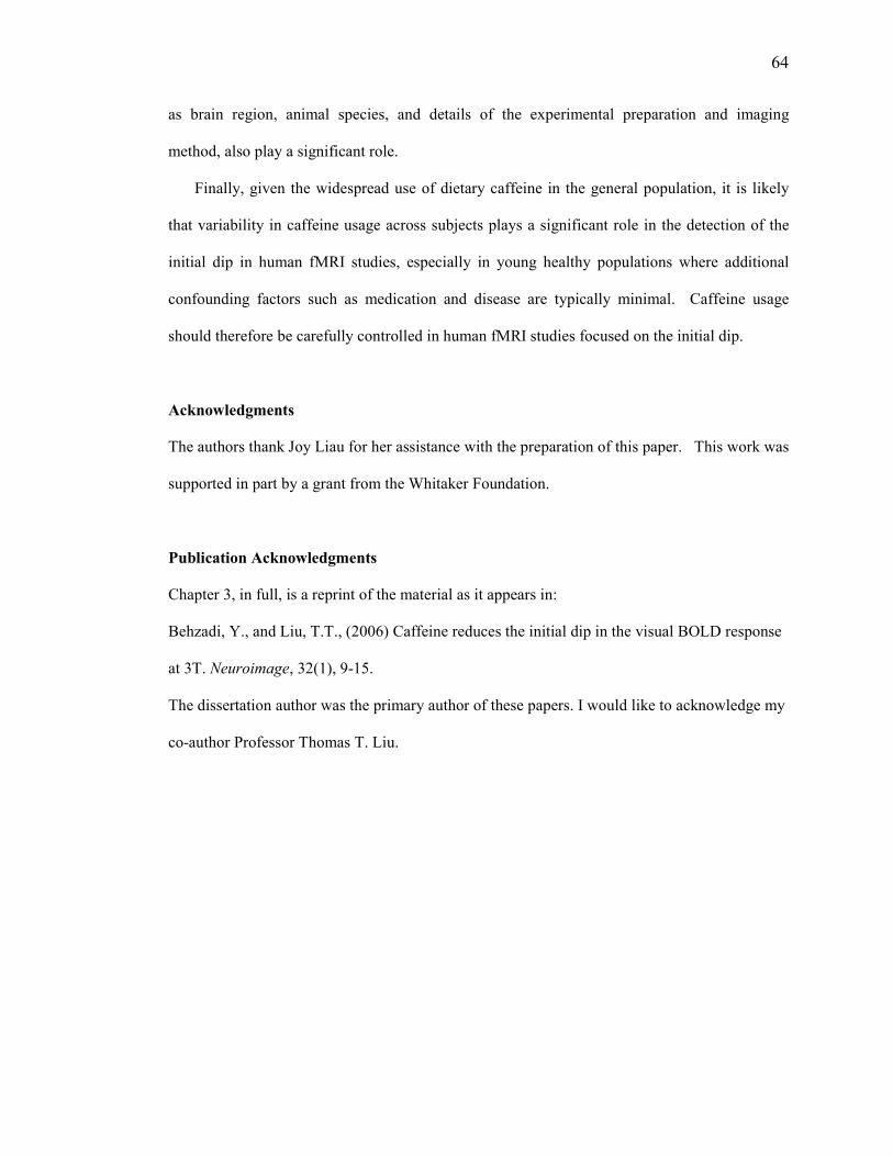
64
as brain region, animal species, and details of the experimental preparation and imaging
method, also play a significant role.
Finally, given the widespread use of dietary caffeine in the general population, it is likely
that variability in caffeine usage across subjects plays a significant role in the detection of the
initial dip in human fMRI studies, especially in young healthy populations where additional
confounding factors such as medication and disease are typically minimal. Caffeine usage
should therefore be carefully controlled in human fMRI studies focused on the initial dip.
Acknowledgments
The authors thank Joy Liau for her assistance with the preparation of this paper. This work was
supported in part by a grant from the Whitaker Foundation.
Publication Acknowledgments
Chapter 3, in full, is a reprint of the material as it appears in:
Behzadi, Y., and Liu, T.T., (2006) Caffeine reduces the initial dip in the visual BOLD response
at 3T. Neuroimage, 32(1), 9-15.
The dissertation author was the primary author of these papers. I would like to acknowledge my
co-author Professor Thomas T. Liu.

65
3.6 Figures
Figure 3.1. Pre-dose (blue) and post-dose (red) group averaged periodic BOLD responses acquired with slice thicknesses of 8mm (panel a) and 4mm (panel c). Averages are from voxels within ROIdip (defined separately for each slice thickness). Magnified views are shown in panels (b) and (d). The initial dip is clearly evident in the pre-dose responses and is absent in the corresponding post-dose responses. The length of each error bar represents the standard error across subjects and the thick black line denotes the stimulus duration.

66
Figure 3.2. Comparison of the post-dose (y-axis) and pre-dose (x-axis) initial dip areas for each subject for voxels within ROIdip. The solid line represents the line of equality. Panels a-c and d-h represent subject data acquired with slice thicknesses of 4 mm and 8 mm, respectively. The p-values were computed with a paired t-test (two-tailed).
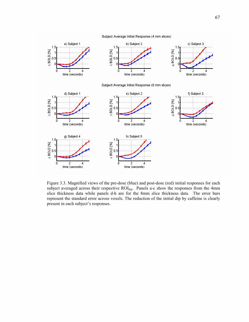
67
Figure 3.3. Magnified views of the pre-dose (blue) and post-dose (red) initial responses for each subject averaged across their respective ROIdip. Panels a-c show the responses from the 4mm slice thickness data while panels d-h are for the 8mm slice thickness data. The error bars represent the standard error across voxels. The reduction of the initial dip by caffeine is clearly present in each subject’s responses.

68
Figure 3.4. Comparison of the pre-dose (top row) and post-dose (bottom row) spatial localization maps for the initial dip (left column) and the positive BOLD response (right column) for subject 1. Panels a) and c) show the spatial extent of the initial dip in the pre-dose and post-dose conditions, respectively, with the colorbar below panel c indicating the scale of the correlation coefficients obtained with the initial dip reference function. Panels b) and d) are positive BOLD spatial maps for the pre-dose and post-dose conditions, respectively. The colorbar below panel d) indicates the scale of the correlation coefficients obtained with the positive BOLD reference function.

69
Table 3.1. Pre-dose and post-dose baseline CBF values shown as mean (standard deviation). Mean and standard deviation were computed across voxels in each subject’s respective ROIdip. For each subject, significance was computed with a paired t test (two-sided).
Subject Estimated daily
caffeine usage
(mg)
Pre-dose
baseline CBF
ml/(100 g min)
Post-dose
baseline CBF
ml/(100 g
min)
Paired t-test
P Value
1 200 53.4 (28.1) 33.5 (16.1) 3.9 e-18
2 <50 57.6 (23.3) 35.1 (16.8) 2.4 e-20
3 200 55.4 (22.6) 38.9 (20.2) 1.7e-11
4 <50 73.1 (14.0) 35.8 (15.9) 1.0e-19
5 250 88.2 (25.2) 47.4 (21.8) 1.8e-19

70
3.7 References
Ances B. M. (2004) Coupling of changes in cerebral blood flow with neural activity: what must initially dip must come back up. J Cereb Blood Flow Metab. 24, 1-6. Ances B. M., Buerk D. G., Greenberg J. H., and Detre J. A. (2001) Temporal dynamics of the partial pressure of brain tissue oxygen during functional forepaw stimulation in rats. Neurosci Lett. 306, 106-110. Behzadi Y. and Liu T. T. (2005) An arteriolar compliance model of the cerebral blood flow response to neural stimulus. Neuroimage. 25, 1100-1111. Buxton R. B. (2001) The elusive initial dip. Neuroimage. 13, 953-958. Buxton R. B., Wong E. C., and Frank L. R. (1998) Dynamics of blood flow and oxygenation changes during brain activation: the balloon model. Magn Reson Med. 39, 855-864. Cameron O. G., Modell J. G., and Hariharan M. (1990) Caffeine and human cerebral blood flow: a positron emission tomography study. Life Sci. 47, 1141-1146. Chalela J., Alsop D. C., Gonzalez-Atavales J. B., Maldjian J. A., Kasner S. E., and Detre J. A. (2000) Magnetic resonance perfusion imaging in acute ischemic stroke using continuous arterial spin labeling. Stroke. 31, 680-687. Cohen E. R., Ugurbil K., and Kim S. G. (2002) Effect of basal conditions on the magnitude and dynamics of the blood oxygenation level-dependent fMRI response. J Cereb Blood Flow Metab. 22, 1042-1053. Cox R. W. (1996) AFNI-software for analysis and visualization of functional magnetic resonance neuroimages. Comput Biomed Res. 29, 162-173. D'Esposito M., Deouell L. Y., and Gazzaley A. (2003) Alterations in the BOLD fMRI signal with ageing and disease: a challenge for neuroimaging. Nat Rev Neurosci. 4, 863-872. Duong T. Q., Kim D. S., Ugurbil K., and Kim S. G. (2000) Spatiotemporal dynamics of the BOLD fMRI signals: toward mapping submillimeter cortical columns using the early negative response. Magn Reson Med. 44, 231-242. Ernst T. and Hennig J. (1994) Observation of a fast response in functional MR. Magn Reson
Med, 146-149. Field A. S., Laurienti P. M., Yen Y.-F., Burdette J. H., and Moody D. M. (2003) Dietary Caffeine Consumption and Withdrawal: Confounding Variables in Quantitative Cerebral Perfusion Studies? Radiology. 227, 129-135. Fransson P., Kruger G., Merboldt K. D., and Frahm J. (1998) Temporal characteristics of oxygenation-sensitive MRI responses to visual activation in humans. Magn Reson Med. 39, 912-919.
71
Fredholm B. B., Battig K., Holmen J., Nehlig A., and Zvartau E. E. (1999) Actions of caffeine in the brain with special reference to factors that contribute to its widespread use. Pharmacol Rev. 51, 83-133. Fukuda M., Wang P., Moon C., Tanifuji M., and Kim S. G. (2005) Spatial specificity of the enhanced dip inherently induced by prolonged oxygen consumption in cat visual cortex: Implication for columnar resolution functional MRI. Neuroimage. in-press. Glover G. H., Li T. Q., and Ress D. (2000) Image-based method for retrospective correction of physiological motion effects in fMRI: RETROICOR. Magn Reson Med. 44, 162-167. Hu X., Le T. H., and Ugurbil K. (1997) Evaluation of the early response in fMRI in individual subjects using short stimulus duration. Magn Reson Med. 37, 877-884. Jones M., Berwick J., Johnston D., and Mayhew J. (2001) Concurrent optical imaging spectroscopy and laser-Doppler flowmetry: the relationship between blood flow, oxygenation, and volume in rodent barrel cortex. Neuroimage. 13, 1002-1015. Kemna L. J. and Posse S. (2001) Effect of respiratory CO(2) changes on the temporal dynamics of the hemodynamic response in functional MR imaging. Neuroimage. 14, 642-649. Kim D. S., Duong T. Q., and Kim S. G. (2000) High-resolution mapping of iso-orientation columns by fMRI. Nat Neurosci. 3, 164-169. Lindauer U., Royl G., Leithner C., Kuhl M., Gold L., Gethmann J., Kohl-Bareis M., Villringer A., and Dirnagl U. (2001) No evidence for early decrease in blood oxygenation in rat whisker cortex in response to functional activation. Neuroimage. 13, 988-1001. Liu T. T., Behzadi Y., Restom K., Uludag K., Lu K., Buracas G. T., Dubowitz D. J., and Buxton R. B. (2004) Caffeine alters the temporal dynamics of the visual BOLD response. Neuroimage. 23, 1402-1413. Logothetis N. K., Guggenberger H., Peled S., and Pauls J. (1999) Functional imaging of the monkey brain. Nat Neurosci. 2, 555-562. Malonek D. and Grinvald A. (1996) Interactions between electrical activity and cortical microcirculation revealed by imaging spectroscopy: implications for functional brain mapping. Science. 272, 551-554. Mandeville J. B., Marota J. J., Ayata C., Moskowitz M. A., Weisskoff R. M., and Rosen B. R. (1999) MRI measurement of the temporal evolution of relative CMRO(2) during rat forepaw stimulation. Magn Reson Med. 42, 944-951. Marota J. J., Ayata C., Moskowitz M. A., Weisskoff R. M., Rosen B. R., and Mandeville J. B. (1999) Investigation of the early response to rat forepaw stimulation. Magn Reson Med. 41, 247-252.

72
Menon R. S., Ogawa S., Strupp J. P., Anderson P., and Ugurbil K. (1995) BOLD based functional MRI at 4 tesla includes a capillary bed contribution: echo-planar imaging correlates with previous optical imaging using intrinsic signals. Magn Reson Med. 33, 453 - 459. Nakao Y., Itoh Y., Kuang T. Y., Cook M., Jehle J., and Sokoloff L. (2001) Effects of anesthesia on functional activation of cerebral blood flow and metabolism. Proc Natl Acad Sci U S A. 98, 7593-7598. Ngai A. C., Coyne E. F., Meno J. R., West G. A., and Winn H. R. (2001) Receptor subtypes mediating adenosine-induced dilation of cerebral arterioles. Am J Physiol Heart Circ Physiol. 280, H2329-2335. Osborne P. G. (1997) Hippocampal and striatal blood flow during behavior in rats: chronic laser Doppler flowmetry study. Physiol Behav. 61, 485-492. Restom K., Behzadi Y., Uludag K., and Liu T. T. (2004) Image Based Physiological Noise Correction for Perfusion-Based fMRI. In: 12th ISMRM Scientific Meeting), pp. 2525, Kyoto. Sicard K., Shen Q., Brevard M. E., Sullivan R., Ferris C. F., King J. A., and Duong T. Q. (2003) Regional cerebral blood flow and BOLD responses in conscious and anesthetized rats under basal and hypercapnic conditions: implications for functional MRI studies. J Cereb Blood Flow Metab. 23, 472-481. Silva A. C., Lee S. P., Iadecola C., and Kim S. G. (2000) Early temporal characteristics of cerebral blood flow and deoxyhemoglobin changes during somatosensory stimulation. J Cereb Blood Flow Metab. 20, 201-206. Thompson J. K., Peterson M. R., and Freeman R. D. (2004) High-resolution neurometabolic coupling revealed by focal activation of visual neurons. Nat Neurosci. 7, 919-920. Vanzetta I. and Grinvald A. (1999) Increased cortical oxidative metabolism due to sensory stimulation: implications for functional brain imaging. Science. 286, 1555-1558. Wang J., M.Qiu, and Constable R. T. (2005) In vivo method for corrrecting transmit/receive nonuniformities with phased array coils. Magn Reson Imaging. 53, 666-674. Wong E. C., Buxton R. B., and Frank L. R. (1998) Quantitative imaging of perfusion using a single subtraction (QUIPSS and QUIPSS II). Magn Reson Med. 39, 702-708. Yacoub E. and Hu X. (2001) Detection of the early decrease in fMRI signal in the motor area. Magn Reson Med. 45, 184-190. Yacoub E., Le T. H., Ugurbil K., and Hu X. (1999) Further evaluation of the initial negative response in functional magnetic resonance imaging. Magn Reson Med. 41, 436-441. Yacoub E., Shmuel A., Pfeuffer J., Van De Moortele P. F., Adriany G., Ugurbil K., and Hu X. (2001) Investigation of the initial dip in fMRI at 7 Tesla. NMR Biomed. 14, 408-412.

73
Chapter 4
CompCor: Component Based Noise Correction for BOLD
and Perfusion fMRI
4.1 Abstract
A component based method (CompCor) for the reduction of noise in both blood
oxygenation level dependent (BOLD) and perfusion-based functional magnetic resonance
imaging (fMRI) data is presented. We show the inclusion of principal components derived from
noise-regions-of-interest (noise ROI) as regressors within the appropriate general linear models
for the BOLD and perfusion-based fMRI time-series data can significantly reduce physiological
noise (e.g. cardiac and respiratory induced fluctuations). In our presentation we investigate the
use of two different methodologies for determining the noise ROI. The first method uses
anatomical data to identify white matter and CSF-only voxels while the second method uses
voxels with high temporal standard deviation to define regions dominated by physiological
noise.
With application of CompCor, the temporal standard deviation of resting state BOLD and
ASL is significantly (p<0.01) reduced compared to no correction in a manner consistent with
application of a previously presented retrospective image based correction scheme,
RETROICOR. Additionally, we show a marked improvement in sensitivity during visual
stimulus as quantified in the number of significantly activated voxels based on an F-statistic
threshold. As compared to RETROICOR, CompCor has the following advantages: 1) does not

74
require external monitoring of physiological activity (such as cardiac or respiratory signals); 2)
can be executed in a fully automated fashion (e.g. does not require user intervention).
75
4.2 Introduction
Over the last decade, blood oxygenation level dependent (BOLD) and perfusion-based
functional magnetic resonance imaging (fMRI) have become indispensable tools for studies of
the working brain. When utilized together, the BOLD and perfusion signal can provide a
quantitative understanding of the metabolic response to neural activity and provide insight into
neurovascular coupling mechanisms (Hoge et al., 1999). However, as the fMRI community has
moved to higher field strengths, physiological noise has become an increasingly important
confound limiting the sensitivity and the application of fMRI studies (Kruger et al., 2001; Liu et
al., 2006).
Physiological fluctuations have been shown to be a significant source of noise in BOLD
fMRI experiments, with even a greater effect in perfusion-based fMRI utilizing arterial spin
labeling (ASL) techniques (Kruger et al., 2001; Restom et al., 2006). Physiological sources of
noise primarily include cardiac pulsations and modulations of the main magnetic field by
thoracic cavity volume changes associated with respiration. Additional sources include blood
flow changes coupled to end-tidal C02 and vasomotion occurring at 0.1 Hz (Dagli et al., 1999;
Glover et al., 2000; Hu et al., 1995).
Approaches to removing cardiac and respiratory related-noise include temporal filtering,
image based retrospective correction (RETROICOR), k-space based correction
(RETROKCOR) and navigator echo based correction (DORK) (Biswal et al., 1996; Glover et
al., 2000; Hu et al., 1995; Josephs et al., 2001; Pfeuffer et al., 2002). More recently,
RETROICOR has been extended to a general linear model (GLM) framework (Lund et al.,
2006) and modified for use in ASL (Restom et al., 2006). A recent adaptation for BOLD based
imaging involved the addition of regressors describing variations in respiratory volume (Birn et
al., 2006).
76
An alternate approach to the use of external measures of physiological activity or specially
modified pulse sequences is to globally subtract average time-courses from regions unlikely to
be associated with neural activity (e.g. ventricles, large vessels, etc.). (Lund et al., 2001;
Petersen et al., 1998). Additionally, component based techniques, utilizing independent
component analysis (ICA) or principal components analysis (PCA), have shown potential in
identifying spatial and temporal patterns of structured noise (Beckmann et al., 2004; McKeown
et al., 2003; Thomas et al., 2002). However, the utility of component based methods has been
limited to BOLD studies with sampling times short enough to clearly differentiate cardiac and
respiratory elements from evoked responses (Thomas et al., 2002) in which case a temporal
band pass filter would be adequate for noise removal.
Here we present and characterize a novel component based method (CompCor) for the
correction of physiological noise in BOLD and perfusion-based fMRI. We show that principal
components derived from noise regions-of-interest (ROI) are able to accurately describe
physiological noise processes in gray matter regions. In our presentation we investigate the use
of two different methodologies for determining noise ROIs. The first method uses anatomical
data to identify white matter and CSF voxels, while the second method uses the temporal
standard deviation (tSTD) of the time-series data to identify voxels dominated by physiological
noise. We show that the use of principal components derived from a noise ROI as regressors in
a GLM of the fMRI signal can significantly reduce the temporal variance in resting state scans
and increase the sensitivity of functional BOLD and perfusion-based studies.
4.3 Theory
4.3.1 CompCor Algorithm
The underlying assumption in the CompCor algorithm is that signal from a noise ROI can
be used to accurately model physiological fluctuations in gray matter regions. The term “noise

77
ROI” refers to areas (e.g. white matter, ventricles, large vessels) in which temporal fluctuations
are unlikely to modulated by neural activity and are primarily a reflection of physiological
noise. The ability to model gray matter physiological noise elements is then predicated on the
coherence between physiological fluctuations in noise ROI and the gray matter. A principal
components analysis (PCA) is used to compactly characterize the time-series data from the
noise ROI. Significant principal components are then introduced as covariates in a general
linear model as an estimate of the physiological noise regressors.
In this paper we investigate the use of two methods for determining the noise ROI. The first
method uses anatomical data to identify voxels that consist primarily of either white matter or
cerebrospinal fluid (CSF). Since neural activation is localized to gray matter, fluctuations in
white matter and CSF regions should primarily reflect signals of non-neural origin (e.g. cardiac
and respiratory fluctuations).
In the second method, voxels with high temporal standard deviation (tSTD) are used to
define a noise ROI. This approach is based on previous preliminary work by Lund et al. in
which areas of high temporal standard deviation were found to correspond to ventricles, edge-
regions, and vessels (Lund et al., 2001). The advantage of this method is that it utilizes the time-
series data to identify a noise ROI without the need for an anatomical scan.
In Figure 1, we present a schematic depicting the basic algorithm in which significant
principal components from a noise ROI are used as physiological noise regressors in the GLM
for the gray matter signal. For functional studies, an added processing step is included in which
a preliminary GLM analysis, using the appropriate design matrix Xh, is used to exclude voxels
from the determined noise ROI with a calculated p-value of less than 0.2. This step is performed
to hedge against the possibility of removing stimulus related fluctuations.

78
4.3.2 General Linear Model for ASL and BOLD
The general linear model of the BOLD signal in gray matter can be represented as
nPcSdXhb +++= [1]
where b represents the measured BOLD data, Xh represents the stimulus response where X is
a kN × design matrix and h is a 1×k vector of hemodynamic parameters. In the case of a
block design, X reduces to a vector containing the smoothed stimulus pattern and h reduces to
a scalar representing the unknown amplitude. Nuisance parameters are integrated in Sd , where
S is a lN × matrix comprised of l nuisance model functions and d is a 1×l vector of
nuisance parameters. We have also added physiological noise terms Pc where P is a mN ×
matrix containing m regressors and c represents the unknown regressor weights. Finally, n
represents the additive noise term.
A general linear model (GLM) for ASL data in gray matter can be written as
nPcSdMXhXhp perfBOLD ++++= [2]
where p is the acquired raw data representing interleaved tag and control images. In this model,
the term modeling perfusion perfXh is modulated by a diagonal matrix, M , consisting of
alternating -1’s and 1’s for the tag and control images, respectively (Mumford et al., 2006;
Restom et al., 2006). The term BOLDXh models a BOLD weighted static tissue component.
In a noise ROI, where we expect no stimulus-related response, the GLM reduces to
nPcSdb ++= or nPcSdp ++= for BOLD and perfusion data, respectively. An
assumption of CompCor is that the significant principal components from the noise ROI can be
used as an estimate estP of the physiological regressors P .
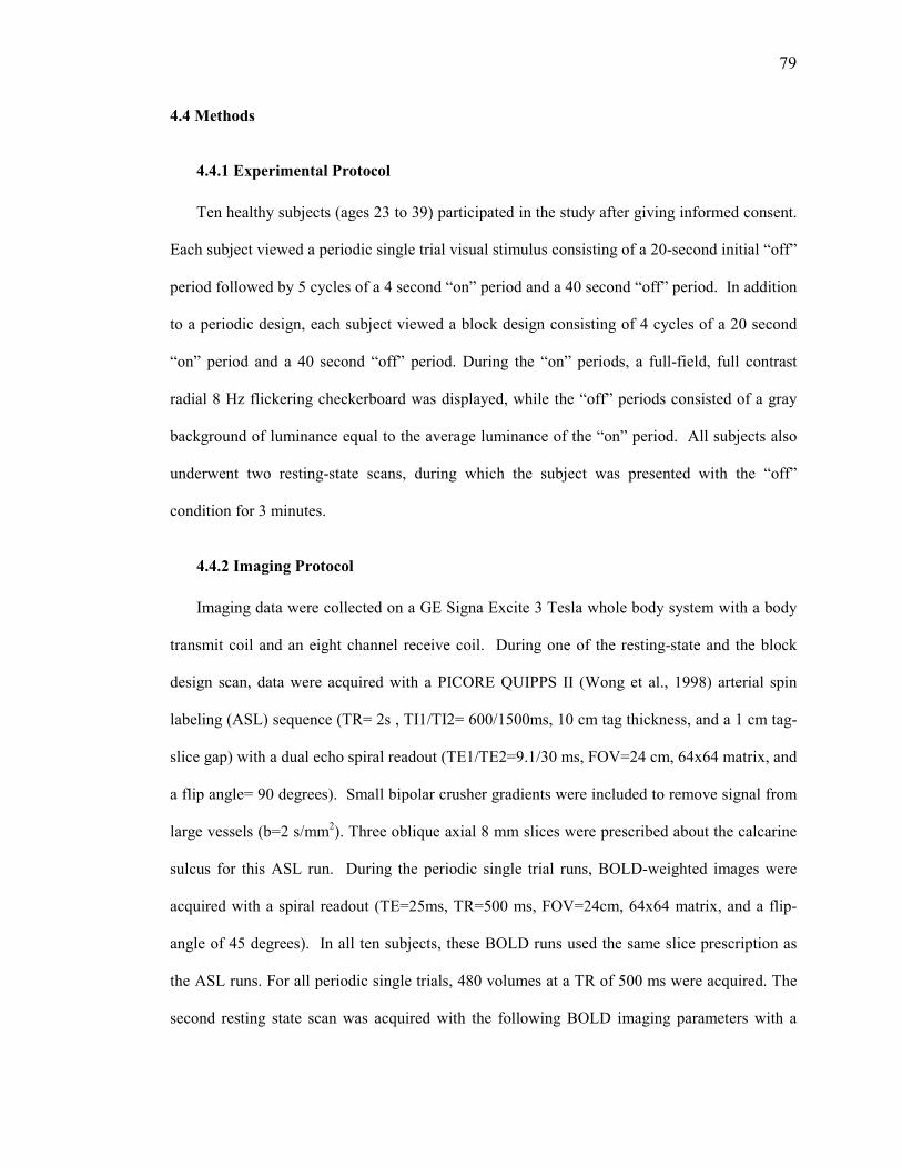
79
4.4 Methods
4.4.1 Experimental Protocol
Ten healthy subjects (ages 23 to 39) participated in the study after giving informed consent.
Each subject viewed a periodic single trial visual stimulus consisting of a 20-second initial “off”
period followed by 5 cycles of a 4 second “on” period and a 40 second “off” period. In addition
to a periodic design, each subject viewed a block design consisting of 4 cycles of a 20 second
“on” period and a 40 second “off” period. During the “on” periods, a full-field, full contrast
radial 8 Hz flickering checkerboard was displayed, while the “off” periods consisted of a gray
background of luminance equal to the average luminance of the “on” period. All subjects also
underwent two resting-state scans, during which the subject was presented with the “off”
condition for 3 minutes.
4.4.2 Imaging Protocol
Imaging data were collected on a GE Signa Excite 3 Tesla whole body system with a body
transmit coil and an eight channel receive coil. During one of the resting-state and the block
design scan, data were acquired with a PICORE QUIPPS II (Wong et al., 1998) arterial spin
labeling (ASL) sequence (TR= 2s , TI1/TI2= 600/1500ms, 10 cm tag thickness, and a 1 cm tag-
slice gap) with a dual echo spiral readout (TE1/TE2=9.1/30 ms, FOV=24 cm, 64x64 matrix, and
a flip angle= 90 degrees). Small bipolar crusher gradients were included to remove signal from
large vessels (b=2 s/mm2). Three oblique axial 8 mm slices were prescribed about the calcarine
sulcus for this ASL run. During the periodic single trial runs, BOLD-weighted images were
acquired with a spiral readout (TE=25ms, TR=500 ms, FOV=24cm, 64x64 matrix, and a flip-
angle of 45 degrees). In all ten subjects, these BOLD runs used the same slice prescription as
the ASL runs. For all periodic single trials, 480 volumes at a TR of 500 ms were acquired. The
second resting state scan was acquired with the following BOLD imaging parameters with a

80
spiral readout (TE=25ms, TR=250 ms, FOV=24cm, 64x64 matrix, and a flip-angle of 40
degrees).
A high resolution structural scan was acquired with a magnetization prepared 3D fast
spoiled gradient acquisition in the steady state (FSPGR) sequence (TI 450ms, TR 7.9ms, TE
3.1ms, 12 degree flip angle, FOV 25x25x16 cm, matrix 256x256x124).
Cardiac pulse and respiratory effort data were monitored using a pulse oximeter (InVivo)
and a respiratory effort transducer (BIOPAC), respectively. The pulse oximeter was placed on
the subject's left index finger, and the respiratory effort belt was placed around the subject's
abdomen. Physiological data were sampled at 40 samples per second using a multi-channel
data acquisition board (National Instruments).
4.4.3 Data Analysis
Preprocessing
All images were coregistered using AFNI software (Cox, 1996) and prewhitened using an
AR1 model prior to subsequent analysis (Burock et al., 2000; Woolrich et al., 2001). An GLM
analysis was then performed using RETROICOR type regressors to construct the physiological
noise matrix, P, as defined in equations 1 and 2 for ASL and BOLD based imaging,
respectively. (Glover et al., 2000; Restom et al., 2006). In addition to statistical inference, this
analysis was used to identify cardiac and respiratory components, which will be used as a basis
for comparison to elements removed by application of CompCor.
Anatomical Definition of Noise ROI
Anatomical data were segmented into gray matter, white matter, and CSF partial volume
maps using the FAST algorithm available in the FSL software package (Smith et al., 2004).
Tissue partial volume maps were linearly interpolated to the resolution of the functional data
series using AFNI (Cox 1996). In order to form white matter ROIs, the white matter partial
81
volume maps were thresholded at a partial volume fraction of 0.99 and then eroded by two
voxels in each direction to minimize partial voluming with gray matter. The erosion process
helps identify deep white matter areas. CSF-only voxels were determined by first thresholding
the CSF partial volume maps at 0.99 and then applying a 3-dimensional nearest-neighbor
criteria to minimize multiple tissue partial voluming. Since CSF regions are typically small
compared to white matter regions mask, erosion was not applied.
CSF and white matter ROIs were combined to form the anatomically defined noise ROI,
subsequently referred to as noise ROIanat. Figure 2 depicts the significant areas of white matter
and cerebrospinal fluid (CSF), as denoted by the magenta voxels, overlayed on their respective
partial volume maps from subject 1.
tSTD Based Determination of Noise ROI
In a preliminary abstract, Lund et al. (2001) showed that voxel time courses with a
relatively high temporal standard deviation were dominated by physiological noise. They
observed that these voxels occurred in edge-regions, ventricles, and in areas close to large
vessels. In their approach, they manually selected five pixels with high temporal standard
deviation that appeared to represent physiological fluctuation. The time-series from these
voxels were then included as nuisance covariates in a GLM, resulting in a marked improvement
in detection power (Lund et al., 2001). Here we extend the prior work by first using the
temporal standard deviation to select voxels in an unsupervised fashion and then using principal
components analysis to reduce the dimensionality of the data. To determine the number of
voxels to include in the ROI, we examined the relation between measures of physiological noise
and measures of temporal standard deviation. For each voxel, we defined the fractional
variance of physiological noise as the ratio of the variance of the time series due to the
physiological noise regressors (as determined with RETROICOR) to the variance of the original
time series (after removal of constant and linear trends). The fractional variance of

82
physiological noise was then compared to the temporal standard deviation on a per-voxel basis.
We denote the ROI identified with this approach as the noise ROItSTD. We found that including
the top 20 voxels per slice based on tSTD provided robust removal of physiological fluctuations
as quantified by the mean reduction in tSTD in gray matter (partial voluming > 0.9) across
subjects for resting BOLD runs. This was based on evaluating the performance of CompCor
with inclusion of 5,10, 20, and 40 voxels per slice. Using 20 voxels significantly outperformed
selecting only 5 and10 voxels but resulted in no significant difference compared to inclusion of
40 voxels. We use a simple selection criteria here to demonstrate proof-of-principle and realize
that more sophisticated and dynamic selection methodologies might result in greater gains.
However, this will be the focus of subsequent work.
Exclusion of stimulus-related components
To further refine the definition of the noise ROI for runs involving functional stimulus, the
voxel time courses within the noise ROI are correlated with the stimulus-related reference
function. Any voxels with a p-value less than 0.2 was excluded from the noise ROI. Numerical
simulations (shown in appendix) indicate that a excluding voxels with a p-value less than 0.2
(R-value <0.1 for block design) with the reference function prevents degradation of
performance due to incorporation of stimulus related fluctuations in the determined prinicipal
components. Here we use an even more conservative threshold to hedge against removal of
stimulus correlated fluctuations.
Determination of Principal Components
Voxels time-series from the noise ROI (either anatomical or tSTD) are placed in a matrix
M with dimensions Nxm , representing the dimensions of time and voxels, respectively. The
constant and linear trends of the columns matrix M are removed prior to column-wise variance
normalization. The covariance matrix, MMC ′= , is constructed and decomposed into its

83
principal components. In our implementation we utilize the singular value decomposition
(SVD) algorithm to perform the PCA, although other algorithms could also be used.
The number of significant principal components is determined using a modified version of
the “broken stick” method described in (Jackson, 1993). This method identifies the point at
which principal values begin to describe mostly random variation in the data. A Monte-Carlo
simulation is first used to generate a statistical representation of expected principal values
derived from normally distributed data of rank equal to the matrix M . This statistical
distribution is then compared to the computed principal values from the data. A threshold is
defined at the point where the difference between the calculated principal values from the data
are no longer significantly different (p<0.05) from the calculated distribution. Based on this
method, we found an average of 6.3± 0.52 and 4.5± 0.38 significant principal components for
BOLD and ASL runs, respectively, when using the anatomical noise ROI. For the noise
ROItSTD ,there were an average of 5.9± 0.74 and 4.2± 0.59 principal components for the
BOLD and ASL runs, respectively.
Quantitative Assessment of Performance
For each subject, average power spectra were obtained by computing the power spectra for
each voxel time-series of interest, averaging the spectra across voxels within the gray matter
voxels (partial volume threshold of 0.9), and then normalizing by the peak power over all
frequencies. The average power spectra of physiological noise components estimated by
RETROICOR was used to identify the peak frequencies related to the cardiac and respiratory
noise elements. Frequencies for which the average cardiac or respiratory components had a
normalized power greater than 0.1 were then used to define cardiac and respiratory frequency
bands, respectively.

84
Spectral coherence analysis was used to compare components removed by RETROICOR
with those removed by CompCor. The average spectral coherence over a frequency band, fband,
is defined (Stoica et al., 1997)
( )bandyybandxx
bandxy
xyfPfP
fPfC
)(
)()(
2
=
where the xxP and yyP are the power spectra of time-series x and y, respectively, and xyP is
the cross power spectral density. For each voxel the spectral coherence across the cardiac and
respiratory bands was computed. The average spectral coherence across voxels in gray matter
(partial volume > 0.9) was then computed.
In order to quantify the degree of noise reduction in the resting state scans, the temporal
standard deviation was computed for all voxels within gray matter (partial volume >0.9). A
paired t-test was then used to assess whether CompCor significantly altered the mean temporal
standard deviation across voxels per subject.
F-statistics were computed using the appropriate GLM for the BOLD and ASL time-series
under the following conditions: 1) no inclusion of physiological noise regressors (e.g. no
correction), 2) inclusion of RETROICOR regressors, 3) inclusion of CompCor regressors
derived from the noise ROIanat, and 4) inclusion of CompCor regressors derived from the noise
ROItSTD. The reference functions, hBOLD and hperf, were formed by convolving the appropriate
stimulus pattern with a gamma density function of the form h(t) = (τn!)− 1((t − ∆t)/τ)
exp(− (t − ∆t)/τ) for t ≥ ∆t and 0 otherwise, with τ = 1.2, n = 3 and ∆t = 1 (Boynton et al., 1996).
A constant term and linear trend term were included as nuisance regressors in the analysis. A
functional region-of-interest was determined for each subject by thresholding the F-values
(corresponding to data with no correction) at 5 and 100, corresponding to p-values of 0.03 and
0.001, for the ASL and BOLD functional runs, respectively. These values were chosen to yield

85
approximately the same number of activated voxels for the ASL and BOLD functional runs and
are consistent with thresholds previously used to investigate physiological noise reduction for
ASL (Restom et al., 2006). A paired t-test was used to assess whether CompCor significantly
increased the number of activated voxels for periodic BOLD and block ASL runs as compared
to no correction on a per subject basis.
4.5 Results
Figure 5 characterizes the elements removed from gray matter regions (partial voluming
>0.9) from the resting BOLD run from subject 1. The normalized average power spectra are
presented. With application of RETORICOR (panel a) cardiac (~1.2 Hz) and respiratory
(~0.2Hz) cpmponents are removed. Application of CompCor using either the noise noise ROIanat
or noise nROItSTD , results in removal of elements consistent with cardiac and respiratory
elements. An additional 1/f component is removed with application of noise ROIanat as depicted
in panel b).
As an example of the noise elements removed with each of the correction schemes,
presented as average power spectra, from Subject 1 are presented in Figure 6. Cardiac and
respiratory elements are aliased due to the long TR and are represented in red and green lines,
respectively. The spectra of elements removed by application of CompCor using the noise ROI
(anat) (panel b) is consistent with cardiac and respiratory elements whereas using the noise ROI
(tSTD) removes primarily a cardiac component (see panel c).
As described in the Methods section, the average spectral coherence for each subject was
computed between noise components identified by CompCor and the cardiac and respiratory
components identified by RETROICOR. For CompCor with noise ROIanat applied to the
resting BOLD runs, the average voxel-wise spectral coherence and standard error values across
subjects (N = 10) were 0.67 ± 0.08 and 0.80 ± 0.05 for respiratory and cardiac elements,

86
respectively. With application of CompCor using noise ROItSTD , average values for the spectral
coherence with respiratory and cardiac elements were 0.62 ± 0.10 and 0.86± 0.07, respectively.
For resting ASL runs the mean spectral coherences when using CompCor with noise ROIanat
were 0.79± 0.03 and 0.65± 0.06 for respiratory and cardiac elements, respectively. With the
application of CompCor using noise ROItSTD , average values for the spectral coherence with
respiratory and cardiac elements were 0.82 ± 0.03 and 0.69± 0.06, respectively. See tables 2
and 3 for a summary of these results.
The impact of CompCor and RETROICOR on the average temporal standard deviation of
the resting BOLD and ASL runs are presented in Figure 7, with associated standard error bars
across subjects (N = 10). Panels a) and b) show the mean temporal standard deviation (tSTD) in
gray matter (partial voluming >0.9) in resting BOLD and ASL, respectively, with application
of RETROICOR and the two variants of CompCor. As compared to no correction,
RETROICOR, significantly (p<0.001) reduced the tSTD in the resting BOLD run from 84.2 to
78.2 whereas application of CompCor using noise ROIanat and CompCor using noise ROItSTD
resulted in even greater reductions to mean values of 63.2 (p<0.001) and 58.4 (p<0.001),
respectively. In resting ASL data the tSTD was reduced from 56.0 to 45.6 (p <0.001), 44.7
(p<0.001), and 42.8 (p<0.001), with the application of RETROICOR, CompCor using noise
ROIanat, and CompCor using noise ROItSTD , respectively.
Bar graphs comparing the effect of the various correction schemes on the number of
activated voxels for the functional ASL block and BOLD periodic runs are shown in Figure 8.
The number of activated voxels for a periodic BOLD run (panel a) was significantly increased
(p<0.001) from 127 to 147.4, 161.2, and 179.9 with the application of RETROICOR, CompCor
using noise ROIanat , and CompCor using noise ROItSTD, respectively. In ASL block functional
runs, the number of voxels passing the F-thresholds increased from 105.9 to 119.6 (p=0.07),
151.1 (p=0.004), and 160.3 (p=0.003) with application of RETROICOR, CompCor using noise

87
ROIanat , and CompCor using noise ROItSTD, respectively. For both functional BOLD and ASL
runs, CompCor using noise ROIanat resulted in greater increases than CompCor using noise
ROItSTD .
4.6 Discussion
In this paper, we have examined whether signal components derived from noise regions of
interest, unlikely to be modulated by neural activity. can be used to reduce the contributions of
physiological noise components within activated regions in the analysis of ASL and BOLD
data. We considered two methods for the determination of the noise ROIs: 1) Anatomical
identification of significant areas of CSF and white matter and 2) Definition of noise regions
based upon their temporal standard deviation. We demonstrated that the application of
CompCor using either ROI significantly reduces the temporal standard deviation of both
resting state BOLD and ASL data. Additionally, we have shown that CompCor with either ROI
leads to a marked improvement in sensitivity during visual stimulus as quantified by the number
of significantly activated voxels for both an ASL block design experiment and a periodic
BOLD design experiment.
In each implementation of CompCor, using either noise ROIanat or noise ROItSTD, there are
possible complications arising from introduction of bias and from the accurate determination of
noise ROI’s. Bias may result in removing components that are related to activation instead of
physiological noise. For instance, although CompCor using the noise ROItSTD resulted in
significant decreases in temporal STD and increases in sensitivity, it relies on the ability to
accurately exclude voxels that may include activation. Accurate exclusion may prove to be
difficult when dealing with complex event-related paradigms for which the expected response
may not be well defined or for resting state scans aimed at studying functional connectivity.

88
Although requiring an additional scan to obtain anatomical data, CompCor using
anatomically defined noise ROI provides an unbiased way of removing physiological
fluctuations, since neural activation should be absent from regions of white matter and CSF.
However, accurate tissue information must be obtained and this can be a concern with various
slice prescriptions or when anatomical to functional alignment is problematic (e.g. due to
subject motion) and result in possible bias. With care, application of CompCor with an
anatomically determined noise ROI, should allow for the robust identification and removal of
physiological fluctuations.
In our implementation of CompCor we use a simplified analysis to determine the number
of significant principal components to retain. Although more sophisticated methods exist to
estimate the latent dimensionality of the noise, we find that the results are fairly insensitive to
the exact number of components used in the GLM.
4.7 Conclusion
We have shown that application of CompCor to ASL and BOLD fMRI time-series can
significantly reduce physiological noise. CompCor does not require external monitoring and can
applied in an automated fashion to reduce the confounding effect of physiological fluctuations
on fMRI time-series.
Acknowledgments
The authors thank Dr. Peter Costandi, Khaled Restom and Dr. Joanna Perthen for their
valued assistance with the preparation of this paper. This work was supported in part by a
Biomedical Engineering Research grant from the Whitaker Foundation and by NIH Grant
R01NS051661.

89
4.8 Appendix . Reduction of Physiological Noise in Simulated fMRI Data
The CompCor algorithm relies on the ability to accurately remove physiological noise
without removing stimulus related fluctuations. In an ideal situation, the noise ROI would only
contain voxels from the noise-only distribution, H0 , and determined principal components
would describe only the noise subspace. However in practice, a percentage of noise ROI voxels
may contain stimulus correlated time-series, taken from a signal+noise distribution H1, and an
exclusion criteria must be used to hedge against removing stimulus correlated components.
Here we examine the effect of the choice of correlation coefficient exclusion criteria on the
resulting performance of CompCor.
The general linear model of the BOLD signal with activation is represented as
nPcSdXhbsimulated +++= [A.1]
where bsimulated represents the overall simulated BOLD response, Xh represents the stimulus
response where X is a kN × design matrix and h is a 1×k vector of hemodynamic
parameters. Nuisance parameters, constant and linear terms, are integrated in Sd and
physiological noise terms in Pc where P is a mN × matrix containing m regressors and c
are unknown regressor weights. Finally, n represents the additive noise term. H1 voxels include
a stimulus response while H0 do not include an Xh term.
As is the case in fMRI data analysis, knowledge of the physiological noise parameters is not
available and GLM analysis is performed using an estimate of the physiological noise
regressors:
ncPdShXb estsimulated +++= ˆˆˆ [A.2]
where the h , d , c and n represent estimates of the true stimulus amplitude, nuisance term,
physiological noise, and residual noise. In this formulation, the physiological noise is not

90
explicitly known so an estimate, estP , is used. In the CompCor algorithm estP is determined by
performing a principal component analysis of noise-only voxels, H0. A threshold based on a
calculated correlation coefficient with the stimulus reference function is used to exclude voxels
that may contain stimulus-related fluctuations. Here we explicitly characterize the ability of the
CompCor algorithm to remove physiological noise as a function of the correlation coefficient
threshold.
A Monte Carlo simulation was used to characterize the CompCor process on removing
known physiological data. Individual voxel responses (N=5000) were generated by randomly
selecting the relative weights of components within the GLM framework. Noise only voxels,
H0, and noise with activation, H1, were generated. Physiological regressors were generated at
frequencies consistent with cardiac (0.9 Hz) and respiration (0.3 Hz) with randomly generated
phases to represent possible phase lags between voxels. Physiological noise weights were
chosen from a distribution governed by N(0,0.3). A constant term was included as a nuisance
term with d chosen from an uniform distribution, U(0,1). The additive noise term, n, were
generated from a normal distribution, N(0,1). For H1 voxels, the stimulus response, Xh, was
generated using a block design, 20 second initial off period followed by 4 cycles of 20 seconds
on and 40 seconds off. The stimulus weight was chosen as 0.3 to simulate a worst-case scenario
with a low-level stimulus response.
The estimation of the physiological noise regressors is determined using a principal
component analysis of voxel time-series below an absolute value of correlation coefficients
(CC). CC’s were determined using the reference function and a simplified version of the GLM
without the inclusion of physiological noise terms, Pc.
Panel a) in figure A.1 is a representation of the resulting histogram of correlation
coefficients using a equal number of H1 and H0 voxels. The solid-line distributions represent the
H0 and H1 without inclusion of physiological noise and the dotted-line distributions reflect the

91
effect of physiological noise on the respective distributions. The H1 distribution is centered on a
correlation coefficient of 0.3 before inclusion of physiological noise and 0.2 after. As expected,
the added noise degrades the calculated CC’s.
If a principal component analysis is performed on the H0 voxel time-series, the
physiological noise subspace can be compactly characterized with the use of only five principal
components. Principal components are used as columns of the estimated physiological noise
matrix estP allowing for the removal of physiological noise. However, in practice we do not
have perfect knowledge of H0 and H1 voxels and a CC threshold must be used to select voxels to
be included in the PCA. As the absolute value of the CC threshold is increased we would
expect more H1 voxels being incorporated in the PCA analysis and the possibility to remove
stimulus-related fluctuations is increased. Panel b) of figure A1, depicts the maximum
correlation of the identified principal components and the reference function. As the CC
threshold increases beyond ~0.2 , the derived PC’s begin to become increasingly more
correlated. Inclusion of the PC’s in the GLM will decrease the estimated stimulus response
weight and degrade performance.
As the CC threshold is increased for inclusion of voxels in the subsequent principal
component analysis, the degree of correction is reduced, as depicted by the ROC curves
provided in panel c) in figure A.1. This is a result of the confounding effects of stimulus related
fluctuations. The dotted line is a representation of the probability of detection (pD) versus the
probability of false alarm (pFa) of the uncorrected data. Using a low CC threshold, in which H1
voxels are excluded from PCA analysis, results in increased pD with a decrease in pFa, as
depicted in the upward shift of the ROC curve. However, at a threshold of 0.16, the resulting
performance of using the correction is worse than the uncorrected data.
Panel d) depicts the area under the ROC curve as a function of CC threshold. This is a non-
parametric normalized measure of performance and it is evident that the overall performance is

92
degraded when using a CC threshold beyond 0.2. However, performance is robust below this
threshold and based on this simulation we choose to use a conservative exclusion criteria of 0.1
in our presentation of CompCor.

93
4.9 Figures and Tables
Figure 4.1. Schematic of the CompCor algorithm in which significant principal components derived from time-series data within noise regions-of-interest are used to form an estimate, Pest, of the physiological noise matrix, P. Incorporation of Pest into the general linear model for gray matter allows for estimation and removal of physiological fluctuations.

94
Figure 4.2. Areas with a high fraction of white matter and cerebrospinal fluid (CSF), as denoted by the magenta voxels, overlaid on their respective partial volume maps from a representative slice from Subject 1. White matter-only areas (panel a) were determined by first thresholding the white matter partial volume fraction map at 0.99 and then performing a map erosion by two pixels to minimize the effect of partial voluming with other tissue types. Panel b) displays CSF-only areas with a partial volume fraction greater than 0.99 with application of a nearest neighbor clustering criteria.

95
Figure 4.3. Panel a) is a spatial map of the fraction of the variance of physiological noise to the overall signal variance for the resting BOLD scan from a representative slice in subject 1. Panel c) compares the log(tSTD) to the fractional variance of physiological noise per voxel. Data points in red represent the twenty voxels with the highest tSTD and correspond to a high fraction of physiological noise. Areas of high fractional variance of physiological noise correspond to areas of high temporal standard deviation (tSTD) of the raw time-series as depicted in panel b).

96
Figure 4.4. Panel a) is a spatial map of the fraction of the variance of physiological noise to the overall signal variance for the resting ASL scan from a representative slice in subject 1. Panel c) compares the log(tSTD) to the fractional variance of physiological noise per voxel. Data points in red represent the twenty voxels with the highest tSTD and correspond to a high fraction of physiological noise. Areas of high fractional variance of physiological noise correspond to areas of high temporal standard deviation (tSTD) of the raw time-series as depicted in panel b).

97
Figure 4.5. Average normalized power spectra of components removed from gray matter (partial volume >0.9) with the application of various correction schemes to the resting BOLD run from subject 1. As shown in panel a, cardiac and respiratory elements removed by RETROICOR are located at 0.2 and 1.2 Hz, respectively. Application of CompCor using either noise ROIanat (panel b) or noise ROItSTD (panel c) removes components similar to the cardiac and respiratory elements identified by RETROICOR. The use of noise ROIanat also removes a 1/f noise component as evident in panel b).

98
Figure 4.6. Average normalized power spectra of components removed from gray matter (partial volume >0.9) with application of various correction schemes to the resting ASL run from subject 1. As shown in panel a, cardiac (red) and respiratory (green) elements identified by RETROICOR are aliased due to the long TR. The power spectra of components removed by application of CompCor using the noise ROIanat (panel b) is similar to the sum of the cardiac and respiratory elements identified by RETROICOR. In contrast, CompCor with the noise ROI (tSTD) removes primarily a cardiac component (see panel c).
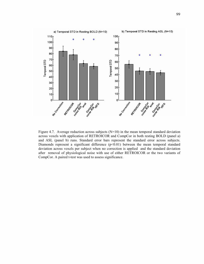
99
Figure 4.7. Average reduction across subjects (N=10) in the mean temporal standard deviation across voxels with application of RETROICOR and CompCor in both resting BOLD (panel a) and ASL (panel b) runs. Standard error bars represent the standard error across subjects. Diamonds represent a significant difference (p<0.01) between the mean temporal standard deviation across voxels per subject when no correction is applied and the standard deviation after removal of physiological noise with use of either RETROICOR or the two variants of CompCor. A paired t-test was used to assess significance.
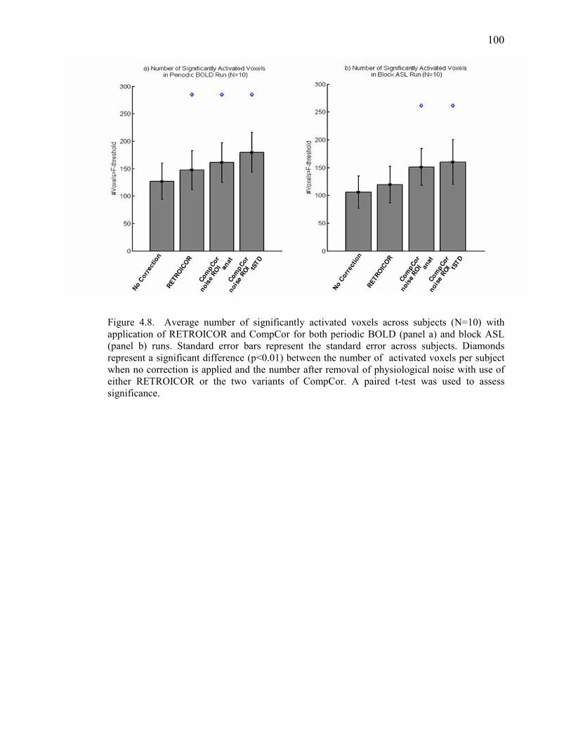
100
Figure 4.8. Average number of significantly activated voxels across subjects (N=10) with application of RETROICOR and CompCor for both periodic BOLD (panel a) and block ASL (panel b) runs. Standard error bars represent the standard error across subjects. Diamonds represent a significant difference (p<0.01) between the number of activated voxels per subject when no correction is applied and the number after removal of physiological noise with use of either RETROICOR or the two variants of CompCor. A paired t-test was used to assess significance.

101
Figure 4.9. Effect of physiological noise and application of CompCor on simulated fMRI responses. Panel a) is a histogram of resulting correlation coefficients between the generated time-series and the reference function. The histograms in blue represent the H0 and H1 distributions without the inclusion of physiological noise. The histograms in red depict the degrading effect of physiological noise on the H1 distribution. Panel b) characterizes the effect of the CC threshold on the derived principal components. As the CC increases stimulus-correlated elements in the principal components become evident. This then results in degradation of performance as shown by the downward shift of the cyan ROC curve with respect to the dotted line representing performance without correction in panel c). Panel d) provides a non-parametric visualization of performance and degradation occurs beyond a CC of 0.15.
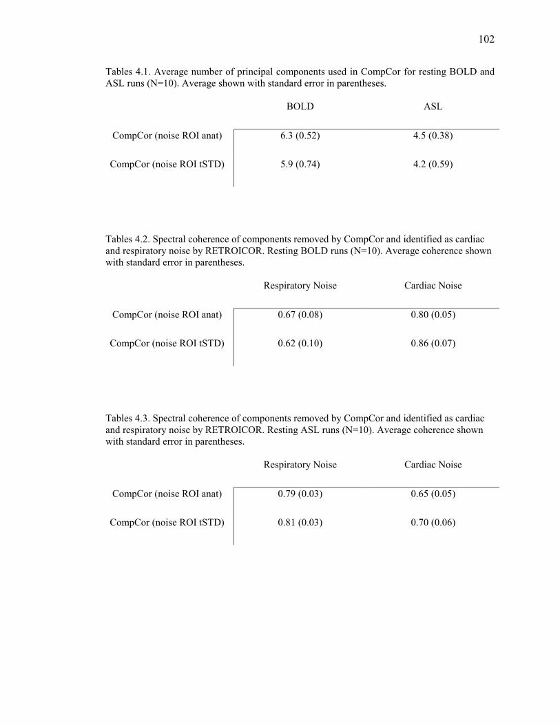
102
Tables 4.1. Average number of principal components used in CompCor for resting BOLD and ASL runs (N=10). Average shown with standard error in parentheses.
BOLD ASL
CompCor (noise ROI anat) 6.3 (0.52) 4.5 (0.38)
CompCor (noise ROI tSTD) 5.9 (0.74) 4.2 (0.59)
Tables 4.2. Spectral coherence of components removed by CompCor and identified as cardiac and respiratory noise by RETROICOR. Resting BOLD runs (N=10). Average coherence shown with standard error in parentheses.
Respiratory Noise Cardiac Noise
CompCor (noise ROI anat) 0.67 (0.08) 0.80 (0.05)
CompCor (noise ROI tSTD) 0.62 (0.10) 0.86 (0.07)
Tables 4.3. Spectral coherence of components removed by CompCor and identified as cardiac and respiratory noise by RETROICOR. Resting ASL runs (N=10). Average coherence shown with standard error in parentheses.
Respiratory Noise Cardiac Noise
CompCor (noise ROI anat) 0.79 (0.03) 0.65 (0.05)
CompCor (noise ROI tSTD) 0.81 (0.03) 0.70 (0.06)

103
4.10 References Beckmann C. F. and Smith S. M. (2004) Probabilistic independent component analysis for functional magnetic resonance imaging. IEEE Trans Med Imaging. 23, 137-152. Birn R. M., Diamond J. B., Smith M. A., and Bandettini P. A. (2006) Separating respiratory-variation-related fluctuations from neuronal-activity-related fluctuations in fMRI. Neuroimage. 31, 1536-1548. Biswal B., DeYoe A. E., and Hyde J. S. (1996) Reduction of physiological fluctuations in fMRI using digital filters. Magn Reson Med. 35, 107-113. Boynton G. M., Engel S. A., Glover G. H., and Heeger D. J. (1996) Linear systems analysis of functional magnetic resonance imaging in human V1. J Neuroscience. 16, 4207-4221. Burock M. A. and Dale A. M. (2000) Estimation and detection of event-related fMRI signals with temporally correlated noise: a statistically efficient and unbiased approach. Human Brain Mapping. 11, 249-260. Cox R. W. (1996) AFNI-software for analysis and visualization of functional magnetic resonance neuroimages. Comput Biomed Res. 29, 162-173. Dagli M. S., Ingeholm J. E., and Haxby J. V. (1999) Localization of cardiac-induced signal change in fMRI. Neuroimage. 9, 407-415. Glover G. H., Li T. Q., and Ress D. (2000) Image-based method for retrospective correction of physiological motion effects in fMRI: RETROICOR. Magn Reson Med. 44, 162-167. Glover G. H., Li T.-Q., and Ress D. (2000) Image-based method for retrospective correction of physiological motion effects in fMRI: RETROICOR. Magn Res Med. 44, 162-167. Hoge R. D., Atkinson J., Gill B., Crelier G. R., Marrett S., and Pike G. B. (1999) Investigation of BOLD signal dependence on cerebral blood flow and oxygen consumption: the deoxyhemoglobin dilution model. Magn Reson Med. 42, 849-863. Hu X., Le T. H., Parrish T., and Erhard P. (1995) Retrospective estimation and correction of physiological fluctuation in functional MRI. Magn Reson Med. 34, 201-212. Jackson D. A. (1993) Stopping Rules in Principal Components Analysis: A Comparison of Heuristical and Statistical Approaches. Ecology. 74, 2204-2214. Josephs O., Howseman A., Friston K. J., and Turner R. (2001) Physiological Noise Modelling for multi-slice EPI fMRI using SPM. Proc Intl Soc Mag Reson Med, 1682. Kruger G. and Glover G. H. (2001) Physiological noise in oxygenation-sensitive magnetic resonance imaging. Magn Reson Med. 46, 631-637.

104
Liu C. S., Miki A., Hulvershorn J., Bloy L., Gualtieri E. E., Liu G. T., Leigh J. S., Haselgrove J. C., and Elliott M. A. (2006) Spatial and temporal characteristics of physiological noise in fMRI at 3T. Acad Radiol. 13, 313-323. Lund T. E. and Hanson L. G. (2001) Physiological Noise Reduction in fMRI Using Vessel Time-Series as Covariates in a General Linear Model. Proc Intl Soc Mag Reson Med. 9, 22. Lund T. E., Madsen K. H., Sidaros K., Luo W. L., and Nichols T. E. (2006) Non-white noise in fMRI: does modelling have an impact? Neuroimage. 29, 54-66. McKeown M. J., Hansen L. K., and Sejnowsk T. J. (2003) Independent component analysis of functional MRI: what is signal and what is noise? Curr Opin Neurobiol. 13, 620-629. Mumford J. A., Hernandez-Garcia L., Lee G. R., and Nichols T. E. (2006) Estimation efficiency and statistical power in arterial spin labeling fMRI. Neuroimage. 33, 103-114. Petersen N., Jensen J., Burchardt J., and Stodkilde-Jorgensen H. (1998) State space models for physiological noise in fMRI time series. Neuroimage. 7, 727-741. Pfeuffer J., Van de Moortele P. F., Ugurbil K., Hu X., and Glover G. H. (2002) Correction of physiologically induced global off-resonance effects in dynamic echo-planar and spiral functional imaging. Magn Reson Med. 47, 344-353. Restom K., Behzadi Y., and Liu T. T. (2006) Physiological noise reduction for arterial spin labeling functional MRI. Neuroimage. 31, 1104-1115. Smith S. M., Jenkinson M., Woolrich M. W., Beckmann C. F., Behrens T. E., Johansen-Berg H., Bannister P. R., De Luca M., Drobnjak I., Flitney D. E., Niazy R. K., Saunders J., Vickers J., Zhang Y., De Stefano N., Brady J. M., and Matthews P. M. (2004) Advances in functional and structural MR image analysis and implementation as FSL. Neuroimage. 23 Suppl 1, S208-219. Stoica P. and Moses R. (1997) Introduction to Spectral Analysis. Prentice-Hall, Upper Saddle River, NJ. Thomas C. G., Harshman R. A., and Menon R. S. (2002) Noise reduction in BOLD-based fMRI using component analysis. Neuroimage. 17, 1521-1537. Wong E. C., Buxton R. B., and Frank L. R. (1998) Quantitative imaging of perfusion using a single subtraction (QUIPSS and QUIPSS II). Magn Reson Med. 39, 702-708. Woolrich M. W., Ripley B. D., Brady M., and Smith S. M. (2001) Temporal autocorrelation in univariate linear modeling of FMRI data. Neuroimage. 14, 1370-1386.
105
Chapter 5
Conclusions
fMRI has grown tremendously over the past decade as a valuable tool to non-invasively
study the working human brain. Although a powerful tool, the fMRI signal is an indirect
measure of neural activity and is the result of the complex coupling of evoked neural responses
and regional hemodynamics. Non-neuronal sources of variability have limited the application
and quantitative interpretation of the fMRI signal. In particular, the baseline vascular state and
physiological noise have remained important factors confounding the fMRI signal.
5.1 An Arteriolar Compliance Model of the CBF Response to Neural Stimulus
5.1.1 Contributions
In chapter 2, a novel arteriolar compliance model was presented and shown to describe to
first order the observed complex dependence of BOLD dynamics on the baseline vascular state.
Published in (Behzadi et al., 2005), the arteriolar compliance model represents the first
concerted effort to model this important effect.
5.1.2 Future Directions
Although the arteriolar compliance model has been shown to predict to first order the
observed changes in the temporal dynamics of the CBF and BOLD responses, it is unable to
simultaneously fit the post-stimulus undershoot of the BOLD response under all baseline
conditions(Behzadi et al., 2005). The post-stimulus undershoot is thought to originate from a
mismatch between CBF and CBV that is a result of the viscoelastic properties of the venous

106
compartment(Buxton et al., 1998). As CBF returns to its baseline value with cessation of
evoked neural activity the CBV remains elevated, returning to baseline with a viscoelastic time
constant for deflation, τv- . Then if the oxygen extraction fraction returns to baseline with CBF,
and the CBV remains elevated, the total dHb will be higher than baseline, reducing the BOLD
signal. However other explanations of the post-stimulus undershoot are possible. CMRO2 may
remain elevated with a return to baseline of CBF and CBV or CBF may drop below baseline
after the stimulus ends, possibly due to neuronal inhibition during the post-stimulus
period(Buxton et al., 1998).
In Behzadi et al., we showed that the τv- appears to decrease with resting CBF(Behzadi et
al., 2005). A smaller τv- at low baseline CBF suggests a relatively greater elastic response. This
may reflect the non-linear nature of the veins in which they are fairly compliant and stiffen
exponentially as the CBF and radius increase(Fung, 1984). Although this result supports the
notion that the post-stimulus undershoot is a reflection of a mismatch between CBF and CBV,
more investigation is required to fully elucidate the role of CMRO2 and neural activity during
this period. Extensions to the arteriolar compliance model are needed to explain the dynamics of
the post-stimulus undershoot.
In order to describe discrepancies between spin echo and gradient echo based BOLD
measurements, Uludag et al. recently presented the compartmental balloon model(Uludag et al.,
2005). In his formulation the BOLD signal model was adapted to describe the various
contribution of the arteriole, capillary, and venules vascular compartments to the overall BOLD
signal. This extension of the balloon model represents an important step in describing
differences in the observed BOLD dynamics as a result of different pulse sequence sensitivities.
Future work will involve integration of the arteriolar compliance model and the compartmental
balloon model.

107
5.2 Caffeine Reduces the Initial Dip in the Visual BOLD Response at 3T
5.2.1 Contributions
In chapter 3, we show that caffeine, through modulation of the baseline vascular state,
significantly affects the detection of the initial dip in the visual BOLD response. As presented in
(Behzadi et al., 2006), this study provides insight into the physiological basis of the initial dip
and on the on-going debate in fMRI regarding the presence of the initial dip that has spanned
several years.
5.2.2 Future Directions
Additional extensions to the BOLD model are needed to help explain the experimental
observation that the initial dip is reduced with vasoconstriction. If strict coupling of CBF and
CMRO2 is preserved, as presented in the formulation of the arteriolar compliance model in
chapter 2, we would expect no initial decrease in dHb. For an initial dip of the BOLD signal to
occur, there must be a transient increase in dHb resulting from a mismatch of CBF and CMRO2
(Behzadi et al., 2006). This may occur if there is a time delay between an immediate change in
CMRO2 and the consequent CBF changes. It is currently unclear what the dependence of the
CMRO2 dynamics are on the baseline vascular state. A more formal metabolic model for
CMRO2 dynamics as a function of baseline is needed and will be the focus of future work.
5.3 Component Based Noise Correction
5.3.1 Contributions
In chapter 4, a component based method for the removal of physiological noise was
developed and shown to significantly reduce the temporal variance and increase the sensitivity
of BOLD and perfusion-based fMRI. The proposed algorithm was shown to remove cardiac and
respiratory induced noise without the need for external monitoring of physiological processes .

108
5.3.2 Future Directions
We presented a component based noise correction scheme in chapter 4 that utilized
principal components from noise regions-of-interest to model and remove the effect of
physiological noise from gray matter. Future extensions to this technique will investigate the
use of independent component analysis (ICA) to identify individual physiological noise
elements. Whereas PCA involves the estimation of uncorrelated (orthogonal) components, ICA
takes a more general approach and aims at decomposing the data into statistically independent
and non-Gaussian components (McKeown et al., 1998). ICA has been used extensively in fMRI
to identify underlying patterns of activation (Beckmann et al., 2004; McKeown et al., 2003;
McKeown et al., 1998). However, its ability to robustly identify the physiological noise
subspace has yet to be studied.
Recently additional sources of physiological noise have been identified involving variations
in respiratory volume and cardiac rate variation (Birn et al., 2006) (Katura et al., 2006).
Additional extensions to the CompCor algorithm presented in chapter 4 will be to characterize
its ability to remove noise components related to variation of the respiratory and cardiac rates
occurring at 0.03 Hz and 0.1 Hz, respectively.

109
5.4 References
Beckmann C. F. and Smith S. M. (2004) Probabilistic independent component analysis for functional magnetic resonance imaging. IEEE Trans Med Imaging. 23, 137-152. Behzadi Y. and Liu T. T. (2005) An arteriolar compliance model of the cerebral blood flow response to neural stimulus. Neuroimage. 25, 1100-1111. Behzadi Y. and Liu T. T. (2005) The Viscoelastic Properties of the Venous Compartment are Dependent on Baseline CBF. In: ISMRM 13th Scientific Meeting), pp. 279, Miami. Behzadi Y. and Liu T. T. (2006) Caffeine reduces the initial dip in the visual BOLD response at 3 T. Neuroimage. Birn R. M., Diamond J. B., Smith M. A., and Bandettini P. A. (2006) Separating respiratory-variation-related fluctuations from neuronal-activity-related fluctuations in fMRI. Neuroimage. 31, 1536-1548. Buxton R. B., Miller K., Frank L. R., and Wong E. C. (1998) BOLD signal dynamics: the balloon model with viscoelastic effects. In: Sixth Meeting, International Society for Magnetic
Resonance in Medicine), pp. 1401, Sydney, Australia. Buxton R. B., Wong E. C., and Frank L. R. (1998) The post-stimulus undershoot of the functional MRI signal. Fung Y. (1984) Biomechanics: Circulation, 2 edn. Springer-Verlag, New York. Katura T., Tanaka N., Obata A., Sato H., and Maki A. (2006) Quantitative evaluation of interrelations between spontaneous low-frequency oscillations in cerebral hemodynamics and systemic cardiovascular dynamics. Neuroimage. 31, 1592-1600. McKeown M. J., Hansen L. K., and Sejnowsk T. J. (2003) Independent component analysis of functional MRI: what is signal and what is noise? Curr Opin Neurobiol. 13, 620-629. McKeown M. J. and Sejnowski T. J. (1998) Independent component analysis of fMRI data: examining the assumptions. Hum Brain Mapp. 6, 368-372. Uludag K. and Buxton R. (2005) The Compartmental Balloon Model. In: 12th ISMRM.), Miami.

110
Appendix A1
Magnetic Resonance Imaging Physics Primer
A1.1 Introduction
In 1936, Pauling and Coryell demonstrated that deoxyhemoglobin (dHb) disrupts a
magnetic field, whereas oxygenated Hb does not (Pauling et al., 1936). This origin of this effect
is that Hb is diamagnetic when oxygenated and paramagnetic when deoxygenated. As a
paramagnetic agent, dHb alters the local magnetic susceptibility, creating magnetic field
distortions within and around blood vessels, and this inhomogenous field produces alterations in
the local magnetic resonance (MR) signal. This phenomenon was not leveraged until Ogawa et
al, in 1990, showed that the MR image of a mouse brain was modulated by the level of inspired
02 (Ogawa et al., 1990). They noted that the presence of dHb, a function of inspired 02, reduced
the local MR signal. They identified the effect as the blood oxygenation level dependent
(BOLD) signal and it was soon after that Kwong et al. first demonstrated a mapping of
activation in the human brain using gradient echo MR imaging during visual stimulation
(Kwong et al., 1992).
In order to gain a qualitative understanding of the BOLD signal, we can use the
experimental observation detailed in the Introduction that with neural activity CBF increases
more than CMRO2, leading to decreases in dHb and an increase in the local BOLD signal. This
basic observation has served as the foundation of fMRI and helped revolutionize neuroimaging.
In order to more quantitatively understand the BOLD signal it is first important to review basic

111
MR physics in the context of the BOLD signal. Interpretation of BOLD measurements is greatly
increased with the application of arterial spin labeling (ASL) techniques used to image the
perfusion response to neural activity. Taken together, the ASL and BOLD signals provide an
added insight into the dynamics of the hemodynamics response to neural activity.
A1.2 The NMR signal
A basic review of MR physics is provided to help in the understanding of the BOLD
response used in fMRI. When an object is placed in a uniform magnetic field, denoted by B0,
the nuclear magnetic dipole tend to align with the field. If the direction of magnetization is
altered from its equilibrium point, with application of an external force, the magnetization will
realign with a given time constant T1.
Another important physical phenomena central to MRI is that certain nuclei (notably
hydrogen) possess an intrinsic magnetic moment and rotate at a frequency proportional to the
magnetic field. This phenomena, known as the nuclear magnetic resonance (NMR), was
discovered in 1946 by two groups: Purcell, Torry, and Pound and Bloch, Hansen, and Packard.
The fundamental equation of magnetic resonance is:
00 Bv γ= [1]
In which the resonant frequency (i.e. Larmor frequency) v0, is a function of the molecule
specific gyromagnetic ratio,γ , and the magnetic field, B0. In a basic NMR experiment, a sample
is placed in a uniform magnetic field and an oscillating RF pulse , generated by an oscillating
current in a nearby coil, is applied. At its resonant frequency, a nucleus can absorb
electromagnetic energy from the RF pulse which can effect the direction of its magnetization.
Therefore if the RF pulse is applied at the resonant frequency of the sample and in a field
orthogonal to B0, the magnetization of the sample will “tip” toward a direction orthogonal to B0,
or equivalently into the transverse plane. In time, the magnetization recovers back to align with

112
Figure A1.1. Longitudinal magnetization with recovery rate of T1. After application of a RF pulse, the longitudinal magnetization is “tipped” onto the transverse plane. The
magnetization then recovers to align with B0.
113
the direction of B0 with a time constant T1. During the recovery period, the molecules are
rotating about the axis of the direction of magnetization. This rotating magnetic field creates a
transient oscillating current, known as the free induction decay (FID), in the coil. The recovery
of the longitudinal magnetization following the 90 degree RF pulse, as governed by exponential
T1 recovery, is depicted figure A1.1. The magnitude of the magnetization in the direction of B0
is referred to longitudinal magnetization whereas the magnetization orthogonal to B0 is known
as transverse magnetization or precessing magnetization. The net precessing magnetization
decays away with a time constant, T2. The reason for this is that the individual dipoles that
contribute to the overall transverse magnetization are not all precessing at the same rate. For
instance, a hydrogen molecule in a water sample will experience randomly varying magnetic
fields due to thermal motion of other hydrogen atoms. In some cases the interaction will speed
up the precession and in other cases slow down the precession causing phase shifts between
individual dipoles. Since the net magnetization is dependent on the coherence of the precession
of individual dipoles the signal will be degraded. The process of phase dispersion and T2 decay
is presented in figure A1.2.
To summarize, the NMR signal is a result of applying a RF pulse to tip the sample
magnetization to an angle, known as the flip angle, to the main magnetic field B0. As the
individual molecules precess and realign with the main field, an oscillating current is generated
in a nearby coil. The resultant signal is a function in time of the longitudinal relation time
constant T1 and the transverse decay constant T2, which are both a function of B0. In a more
complex sample, the resultant signal is a function of time determined by multiple T1’s and T2’s.
In practice, the transverse magnetization decays faster than the expected T2. This increased
decay is due to magnetic field inhomogeneity and is referred to T2*. In order to describe the
NMR signal, Block proposed a set of three coupled differential equations. The equations are
written separately for each direction of the magnetization, Mx, My, and Mz.
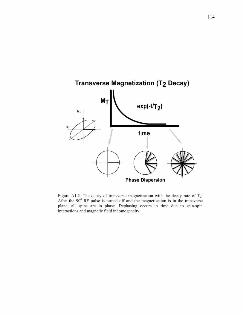
114
Figure A1.2. The decay of transverse magnetization with the decay rate of T2. After the 900 RF pulse is turned off and the magnetization is in the transverse plane, all spins are in phase. Dephasing occurs in time due to spin-spin
interactions and magnetic field inhomogeneity.

115
1
0
2
0
2
0
T
MM
dt
dM
T
MMB
dt
dM
T
MMB
dt
dM
zz
y
x
y
xy
x
−−=
−−=
−=
γ
γ
[2]
In this formulation, Mz is the direction of the main magnetic field B0, and Mx and My are the
directions orthogonal to B0.
A1.3 Magnetic Resonance Imaging
In MRI the hydrogen molecule is used as a basis for generating the NMR signal. Contrast is
generated by taking advantage of the fact that the T1 and T2 of various tissues are different. For
instance, at a B0 of 1.5T, the T1’s for gray matter, white matter, and CSF are 900ms, 700ms, and
4000ms, respectively(Buxton, 2002). The T2’s are considerably shorter at 70 ms, 90 ms, and
400 ms, for gray matter, white matter, and CSF, respectively(Buxton, 2002). Due to the
difference in the T1 and T2’s, contrast between tissue types can be generated by adjusting the
time in which one records the resultant NMR signal. However, the acquired signal has no
information about the location of the source of the signal. Some form of spatial encoding must
be done to localize the acquired signal.
Lauterbaur (1973) and Mansfield (1977) applied a magnetic gradient across a sample in
order to spatially localize the NMR signal (Lauterbur, 1973; Mansfield, 1977). Since the
resonant frequency is dependent on the magnetic field, the molecules in a sample under a
gradient would precess at different rates depending on their location. In other words, a gradient
field produces a linear variation of the precession rate with position. This effect can be
understood by dividing a sample in the direction of the gradient into three distinct regions
denoted by their position relative to the center as x-1, x0, x1. Since the gradient is linear with
respect to location, the local field in each subsection of the sample can be thought as B0-∆B, as
116
B0 ,and, as B0+∆B. At time equal to zero, the net phase of the magnetization in each section is
equivalent. However in time, the phase of x-1 will lag with respect to x0 while x1 will be ahead
due to their different respective magnetic fields. The application of a gradient is modulating the
phase of the localized signal. This modulation is equivalent to multiplying the local signal with
a cosine with a given frequency, which is a function of the length of time the local phase has
been affected by the gradient. The basis of imaging using the NMR signal is the fact that the
phase of the local signal can be manipulated by the application of a magnetic gradient such that
the net signal is the spatial Fourier transform of the distribution of transverse magnetization. If
encoding is performed in multiple directions the resultant NMR signal can be localized in space.
This is more formerly characterized by considering a signal, S(t), within a sample volume
V:
∫ −=V
trirderptS
3),()()( φ [3]
where p(r) is the position dependent density of nuclear spins and ),( trφ represents their phase.
The phase of the signal increases at a rate proportional to its angular velocity, which is turn is a
function of the local magnetic field. With application of a magnetic field gradient, described
by rtGBtrB ⋅+= )(),( 0 , the relative phase between spins can be expressed by:
rtkrdttGtr
t
⋅=⋅
= ∫ )()(),(
0
''γφ [4]
Combining equations 3 and 4, yields
∫ ⋅−=V
rtikrderpkS
3)()()( [5]
which is the Fourier transform equation, stating that S(k) is equivalent the Fourier transform of
the spin density p(r). The net area under the curve of the gradient then determines the relative
position in k-space. A basic MRI image is formed by applying a RF-pulse to tip the

117
Figure A1.3. (a) Schematic echo planar Gx and Gy gradients.
(b)Corresponding trajectory through k-space.

118
magnetization to a given flip angle, α, one then waits a given echo time (TE) depending on
desired contrast, and finally applies gradients and then samples the resultant k-space
representation of the image. The raw data is then the spatially encoded spin density, at an
imaging time with contrast determined by the T1’s, T2’s. Reconstruction of the image is
accomplished by taking the inverse Fourier transform of the image with knowledge of the k-
space trajectory. The process of applying an RF and imaging is repeated at a given time of
repetition, TR.
A basic echo planar imaging (EPI) scheme is presented in figure A1.3. EPI is a time
efficient way to traverse k-space. After slice selective excitation, a negative Gx and Gy gradient
is applied to acquire the first sample in k-space. Recall that the net area under the curve of the
gradients represents the relative encoding of the image and position in k-space. Next a positive
Gx gradient is used to march across kx in which discrete samples are taken from the resultant
NMR signal. A positive Gy gradient is used to move positively in ky and the Gx gradient is
reversed to traverse back across kx. This sequence is repeated until the required k-space
samples are captured. The primary focus of MRI has been in the manipulation of this basic
sequence of events to optimize different contrast of interest in the context of the trade-off
between spatial and temporal resolution.
A1.4 Applications to Functional Imaging
Especially relevant to the discussion of the BOLD signal used extensively in fMRI is the
concept of magnetic susceptibility. Magnetic susceptibility refers to degree to which a material
becomes magnetized when placed in a magnetic field. In addition to the forces discussed earlier,
another effect of placing a sample in a magnetic field is that the local magnetic field is distorted
by the interaction of internal dipole moments in the material with the field. The effective
magnetic field around an object is then distorted by the geometry and susceptibility of that
object. These distortions alter the local magnetic field and thus the resonant frequency of the

119
hydrogen molecule. Difference in susceptibility between different types of materials in the brain
can cause signal reductions. For instance, sinus cavities filled with air can cause field distortions
that negatively affect the surrounding MR signal. These unwanted distortions are further
exaggerated with certain types of imaging sequences. Ironically, although susceptibility effects
have been the cause of much grief in MRI they form the basis of BOLD based fMRI. The
BOLD effect is the result of the differences in magnetic susceptibility of oxygenated and
deoxygenated blood in a vessel. Figure A1.4 is a schematic of a magnetized cylinder in which
the presence of deoxyhemoglobin within the vessel causes magnetic field distortions in the
surrounding space. This then increases the degree of phase dispersion, decreasing the T2*, and
reducing the resulting MR signal.
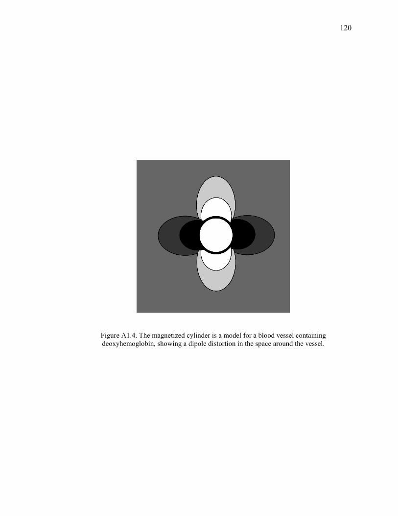
120
Figure A1.4. The magnetized cylinder is a model for a blood vessel containing deoxyhemoglobin, showing a dipole distortion in the space around the vessel.

121
A1.5 References
Buxton R. B. (2002) Introduction to Functional Magnetic Resonance Imaging. Cambridge University Press, Cambridge. Kwong K. K., Belliveau J. W., Stern C. E., Chesler D. A., Goldberg I. E., Poncelet B. P., Kennedy D. N., Weisskoff R. M., Cohen M. S., Turner R., Cheng H.-M., Brady T. J., and Rosen B. R. (1992) Functional MR imaging of primary visual and motor cortex. JMRI. 2(P) [Abstr.], 76. Lauterbur P. C. (1973) Image formation by induced local interactions: examples employing nuclear magnetic resonance. Nature. 242, 190-191. Mansfield P. (1977) Multi-planar image formation using NMR spin echoes. J Phys. C10, L55-L58. Ogawa S. and Lee T.-M. (1990) Magnetic resonance imaging of blood vessels at high fields: in vivo and in vitro measurements and image simulation. Magn Reson Med. 16, 9-18. Pauling L. and Coryell C. D. (1936) The magnetic properties and structure of hemoglobin, oxyhemoglobin, and carbonmonoxyhemoglobin. Proc Natl Acad Sci USA. 22, 210-216.

122
Appendix A2
fMRI: Phyiological Basis
A2.1 Neural System
Neurons are the functional subunits of the brain and their coordinated function results in the
seemingly limitless information processing capability of the human brain. A stark, simple view
of population neuronal processing was put forward in 1943 by McCullough and Pitts in which
all synaptic inputs converged into a single point neuron (McCulloch et al., 1943). In this model
individual neurons would respond to specific environmental or internal inputs and then
broadcast their response, via action potentials, to their postsynaptic targets. Summation of
incoming spikes from multiple neurons would occur at each target neuron and if a given
threshold was exceeded, the target neuron would generate a spike in response. McCullough and
Pitts proved that a sufficiently large number of these simple logic devices, wired appropriately,
would be capable of universal computation (McCulloch et al., 1943). This simple model
provided insight into the importance of the coordinated function and the interconnectivity of
neurons as a basis for their ability to process information. The brain then utilizes this
information according to two fundamental principles of functional specialization and
integration. Specialization refers to the localization of specific types of processing to
anatomically distinct areas of the brain. Integration then refers to the interconnectivity of these
specialized regions.
One of the most well studied areas in the human brain is the visual system located in the
occipital lobe. A brief exploration of the visual system will help highlight the role of

123
specialization and integration in the processing of information. Once visual information is
captured in the eye it is transmitted via the optic nerve to the lateral geniculate nucleus (LGN)
in the thalamus. The V1 region of the visual cortex then receives input directly from LGN.
Specialization is well illustrated in V1, where the visual scene is spatially encoded in a highly
conserved and specific manner. For example, the upper bank of the calcarine sulcus responds to
the lower half of the visual field whereas the lower bank responds to the upper half of the visual
field (Belliveau et al., 1991).
V1 is responsible for the neuronal processing of spatial frequency, orientation, motion,
direction, speed, and other visual features . Strong feedforward connections exist between V1
and V2 and serve to carry and integrate information from V1 for further processing. V2 is tuned
for processing of complex patterns and has connections to V3, V4, and V5 and send feedback
connections back to V1. In addition to environmental inputs from the eyes, the visual system is
modulated by internal sources such as attention pathways. The interconnectivity of the visual
system exemplifies the role of information integration from specialized regions in overall
information processing.
In fMRI applications, the localized neural activity can be simply modeled as a inhibitory
feedback system, in which the neural response U(t) is treated as the sum of excitatory E(t) and
inhibitory inputs I(t). The inhibitory response is driven by the neural response and can be
represented by:
)()()( tItEtU −= [1]
1
)()(
τκ tItU
dt
dI −= [2]
where κ and 1τ are a gain factor and time constant, respectively(Buxton et al., 2001).This
simple linear model allows for the incorporation of neural adaptation and refractory effects
demonstrated experimentally. An nonlinear component may also be introduced to more

124
accuratley capture observed dynamics. By introducing a baseline level of neural activity and
requiring the neural activity to be always positive , one can prevent post-stimulus undershoots
that may occurr in the linear model presented above. This behavior matches a pattern originally
proposed to describe BOLD signal nonlinearities observed in the visual cortex (Boynton et al.,
1996). The necessity of a refractory period has also been proposed to model the diminsihing
response to a pair of closely spaced stimuli (Buxton et al., 2004).
Neural activity leads to increases in tissue metabolism and the firing of neuronal action
potentials result in (1) the release of neurotransmitter into the synaptic cleft and (2) changes in
ionic gradients(Buxton, 2002). Consequently the main cost of maintaining homeostasis
involves the restoration of ionic gradients and repacking of neurotransmitter molecules.
Weighing approximately 3 lbs, the brain uses nearly 20% of the body’s energy and its demands
are met almost exclusively by glucose oxidation, in which 90% of resting glucose consumption
is oxidative (Buxton, 2002). Since the energy yield of glucose oxidation is much more than
glycolysis nearly all the ATP production in the resting state is via glucose oxidation(Buxton,
2002).
Figure A2.1 is a representation of the cellular events associated with the cycling of
glutamate, a neurotransmitter. It is important to note that ATP is used to extrude Na+ taken in
along with glutamate from the synapse, convert glutamate to glutamine, and supply energy to
the Na+/K+ pump used to restore ionic potentials. ATP is primarily supplied by aerobic
glycolysis in astrocytes and the excess lactate is transported to adjacent neurons to be further
metabolized (Raichle et al., 2006).
PET studies by Fox et al. reported that the CMRO2 and for cerebral metabolic rate of
glucose (CMRGlu) is in a ~4:1 molar ratio further supporting the dominant role of oxidative
mechanisms during rest(Raichle et al., 2006). With functional activation, CMRO2 is increased
by only ~15% whereas CMRGlu and CBF are increased ~50% (Raichle et al., 2006).

125
Figure A2.1. A representation of the metabolic events associated with the release of glutamate. It is important to note the role of the astrocyte in supplying ATP for the conversion of glutamate to glutamine, Na+\K+ pump, and the reuptake of glutamate from
the synapse. Based on figure from (Raichle et al., 2006).

126
A2.2 Hemodynamic System
Increases in CBF during activation serve to deliver needed nutrients (e.g. glucose and
oxygen) and carry away byproducts of metabolism (e.g. lactate, heat). The ratio between
relative changes in CBF with respect changes in CMRO2 with neural activity is used as a
parameter describing neurovascular coupling (n) and is denoted (Buxton et al., 2004):
1
1
0,22
0
−−
=∆
∆=
m
f
CMROCMRO
CBFCBFn [3]
Where f and m are CBF and CMRO2 normalized to their respective baseline values. This
fundamental ratio forms the basis of fMRI. The basic picture of brain activation is simple:
stimuli evoke increased activity in neuronal populations, ATP consumption increases, oxidative
metabolism increases to restore ATP, and CBF increases to supply nutrients and carry away
metabolic byproducts. However, the mechanisms involved are complex. A recent review by
Iadecola summarizes the role of activity-induced signaling mechanisms that not only involve
neurons but also astrocytes and vascular cells. Dilation of arterioles resulting from increased
neural activity is dependent on Ca2+ oscillations in astrocytes (Iadecola, 2004). In addition,
upstream vasodilation may result from intramural signaling in endothelial and smooth muscle
cells. Despite the complete understanding of the exact mechanisms involved, it is known that
various vasoactive agents are released following increases in neural activity that modulate the
local cerebral blood flow through their effect on smooth muscle cells(Iadecola, 2004). Several
models have been introduced to describe the CBF response to neural stimulus, most relevant to
fMRI is a model by Friston et al, who presented a simple linear second-order system to describe
the regulation of CBF following neural activity (Friston et al., 2000).
Hemodynamic changes involve the coupling of changes in CBF with cerebral blood volume
and CMRO2. As the smooth muscle relaxes in response to the release of vasoactive agents, the
resistance in the vascular tree decreases. As the resistance decreases, the pressure drop across
127
the vessels also decreases, raising the pressure in both the capillaries and veins. The vessels
expand, increasing the cerebral blood volume. The steady-state relationship between CBF and
CBV is described by (Grubb et al., 1974):
αfv = [4]
where v and f are CBV and CBF normalized by their initial values, respectively. Grubb
experimentally found that α equal to 0.38 which is in contrast to a laminar flow assumption in
which α should equal 0.5 (Grubb et al., 1974). An analytical solution for Grubb’s empirical
relationship can be derived by noting that the total blood volume is the sum of arteriole (Va),
capillary(Vc), and venous blood volumes(Vv) as denoted.
vcaT VVVV ++= [5]
The relationship between volume and flow in the arterial and venous compartments is governed
by a power law relationship with the assumption of laminar flow, αL=0.5. In contrast, during
increases in flow, the capillary compartment experiences negligible increases in volume(Fung,
1984). Substituting expressions for the blood volume in terms of flow using the following
relationships:
( ) LFFVV aa
α00, /= ( ) LFFVV vv
α00, /= ( ) TFFVV TT
α00, /= 0,cc VV = [6]
and solving for αT yields the analytical expression for Grubb’s constant:
)/)//((log 0,0,0,0,0,0, TcTvTafT VVVVVVf L ++= αα [7]
Where f is the normalized flow to its baseline value. Using fractional blood volumes of 0.33,
0.46, and 0.21 for the arterial, venous, and capillary compartments(Oja et al., 1999) ,
respectively, and a physiological change in f of 50% yields a αT of 0.41. This is similar to the
experimental value of 0.38 found by Grubbs.
By definition, the CMRO2 is a function of the oxygen extraction fraction E, the arterial
oxygen concentration Ca, and the CBF, as represented by(Buxton et al., 2004):

128
CBFCECMRO a ⋅⋅=2 [8]
one can also show that the steady-state deoxyhemoglobin concentration [dHb] depends on
CMRO2 and CBF, from basic mass conversation(Hoge et al., 1999):
CBF
CMROdHb 2
4
1][ = [9]
which can also be rewritten in terms of the normalized oxygen extraction fraction as
00,2
02
0][
][
E
E
CMRO
CBF
CBF
CMRO
dHb
dHb=⋅= [10]
If CMRO2 is held constant, the baseline [dHb] term is inversely proportional to the normalized
CBF by
CBF
CBF
dHb
dHb 0
0][
][= [11]
Combining equation 3 and 10, in order to quantify dHb changes with changes in CMRO2 and
CBF, leads to the expression:
nf
nf
dHb
dHb 1
][
][
0
−+= [12]
From experimental observation n>1, typically in the range 2-3, which means that concentration
of dHb would decrease with activation. The total dHb is then determined as the product of the
CBV and dHb concentration. Incorporating Grubb’s relationship, equation 4, with equation 12,
the total amount of dHb can be quantified by:
1
0
1 −⋅−+
= αf
n
nf
dHb
dHb [13]
We are left with the following picture of the associated hemodynamics following neural
activation: With activation, the CBF flow is increased much more than the CMRO2, which leads
to increased CBV and decreases in dHb. It was the discovery that dHb modulates the MR
129
signal,as discussed in Appendix A1, that serves as a foundation for fMRI. The previously
outlined cascade of events following evoked neural activity is illustrated in figure 1.2 of the
Introductory chapter.
A2.3 BOLD Signal
In their pioneering work in 1990, Ogawa et al. found that when the mouse breathed 100%
O2, the brain was rather uniform (Ogawa et al., 1992). However, when the mouse breathed 20%
O2 many dark lines appeared and were localized to vessels. They also noted that the signal loss
was greater with increased TE, suggesting that the presence of deoxygenated blood was acting
on reducing the T2*, and equivalently increasing the R2*, of the blood (Ogawa et al., 1992).
Boxerman et al. later determined that R2* was related to CBV and [dHb], according to
(Boxerman et al., 1995):
βv
dHbdHbCBVAR ][*
2 ⋅⋅= [14]
where β is a constant depending on blood volume and the tissue sample, A is a proportionality
constant, and vdHb][ is the dHb concentration in the venous compartment. Changes in dHb
R*
2
lead to changes in signal intensity as a function of TE by the following expression:
1*,2
0
−=∆ ∆⋅− dHbRTE
eBOLD
BOLD [15]
which for small changes in dHb
R*
2 can be linearized to
*
,2
0
dHbRTEBOLD
BOLD∆⋅−=
∆ [16]
where )][][( 00
*
,2
ββvvdHb dHbCBVdHbCBVAR −⋅⋅=∆ [17], substituting the expression for
dHbR
*
2∆ into equation 16 and non-dimensionalizing yields

130
−⋅=
∆β
000 ][
][1
v
v
dHb
dHb
CBV
CBVM
BOLD
BOLD [18] where M represents the maximal BOLD
signal and is equal to β00 ][ vdHbCBVATEM ⋅⋅⋅= (Hoge et al., 1999). Hoge et al. presented a
method for calibrating the BOLD signal with administration of CO2 (Hoge et al., 1999). Since
CO2 modulates both resting CBF and BOLD without changes in CMRO2 it can be used to
determine the scaling factor M. Without changes in CMRO2, the [dHb] is determined by eq 11,
given by.
CBF
CBF
dHb
dHb 0
0][
][= [19]
Substituting the above expression into eq. 18 along with Grubb’s equation relating CBV and
CBF changes, eq 4, and solving for M yields the expression:
βα −
−
∆
=
0
0
1CBF
CBF
BOLDBOLD
M [20]
With determination of M it is possible then to calculate CMRO2 changes with a functional
paradigm. This equation and CO2 calibration methodology has proved very useful in
interpretating steady-state fMRI experiments.
A2.4 BOLD Signal Dynamics
In the appendix section of chapter two a dynamic model of the BOLD signal was presented.
Here we revisit the presented model and discuss some of its characteristics. Recall
that the flow out of the venous compartment is governed Grubb’s relationship with viscoelastic
effects as defined by
dt
dvvtf vout τα += /1)( [21]

131
Figure A2.2. Dynamic response of the physiological quantities underlying the BOLD signal. The BOLD signal is a function
of [dHb] and CBV which are driven by evoked responses of CBF and CMRO2.

132
the volume (v) and concentration of deoxyhemoglobin (q) are dynamically defined by a
−
−+=
−=
v
qf
n
nf
dt
dq
ffdt
dv
out
in
outin
11
)(1
0
0
τ
τ [22]
where 0τ is the mean transit time, n is the coupling parameter, and inf is the flow into the
venous compartment as determined by the arteriolar compliance model. The BOLD signal is
then determined by a signal model (Chapter 2, Eq. A17) that is a function of the state variable v
and q along with constants determined by imaging parameters.
Figure A2.2 is a schematic representing the dynamics response of the various physiological
parameters underlying the BOLD effect in fMRI. A stimulus, in this case represented by a block
of activity, drives a neural response which reaches a peak and slowly decays as governed by
equations 1 and 2. The neural activity modulates the CBF response through the release of a
vasoactive agent that acts on the smooth muscle compliance as governed by the arteriolar
compliance model put forward in Chapter 2. The CBF response serves as an input into the
balloon model which predicts the temporal time courses of CBV and the dHb content. The
CMRO2 response is a reflection of the CBF response since a linear coupling was assumed.
However, we delay the CBF response relative to the CMRO2 to reveal the initial dip in the
depicted BOLD response. With cessation of activation the CBF response returns back to
baseline but the CBV response remains elevated due to the viscoelastic properties of the venous
compartment. The temporal mismatch between the CBF and CBV response leads to an
accumulation of dHb and a post-stimulus undershoot in the BOLD response. This schematic is
helpful in understanding the complicated interplay of the various physiological parameters
governing the dynamics of the evoked BOLD response.
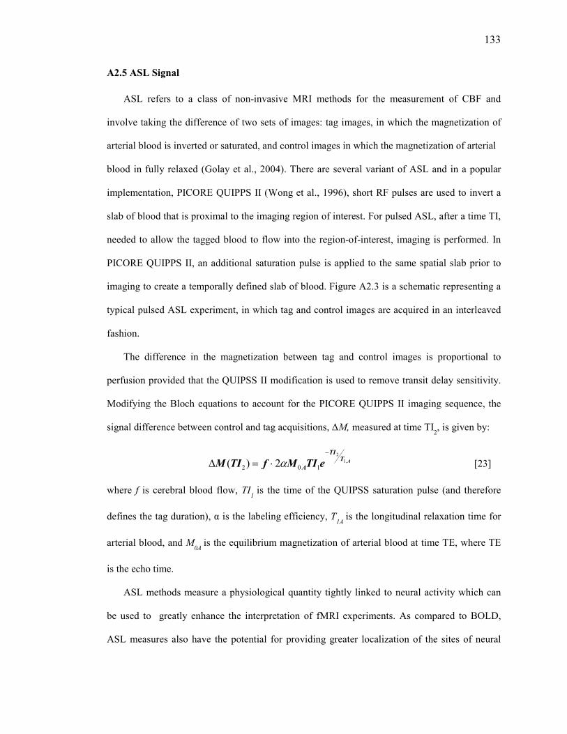
133
A2.5 ASL Signal
ASL refers to a class of non-invasive MRI methods for the measurement of CBF and
involve taking the difference of two sets of images: tag images, in which the magnetization of
arterial blood is inverted or saturated, and control images in which the magnetization of arterial
blood in fully relaxed (Golay et al., 2004). There are several variant of ASL and in a popular
implementation, PICORE QUIPPS II (Wong et al., 1996), short RF pulses are used to invert a
slab of blood that is proximal to the imaging region of interest. For pulsed ASL, after a time TI,
needed to allow the tagged blood to flow into the region-of-interest, imaging is performed. In
PICORE QUIPPS II, an additional saturation pulse is applied to the same spatial slab prior to
imaging to create a temporally defined slab of blood. Figure A2.3 is a schematic representing a
typical pulsed ASL experiment, in which tag and control images are acquired in an interleaved
fashion.
The difference in the magnetization between tag and control images is proportional to
perfusion provided that the QUIPSS II modification is used to remove transit delay sensitivity.
Modifying the Bloch equations to account for the PICORE QUIPPS II imaging sequence, the
signal difference between control and tag acquisitions, ∆M, measured at time TI2, is given by:
ATTI
A eTIMfTIM ,1
2
102 2)(−
⋅=∆ α [23]
where f is cerebral blood flow, TI1 is the time of the QUIPSS saturation pulse (and therefore
defines the tag duration), α is the labeling efficiency, T1A
is the longitudinal relaxation time for
arterial blood, and M0A
is the equilibrium magnetization of arterial blood at time TE, where TE
is the echo time.
ASL methods measure a physiological quantity tightly linked to neural activity which can
be used to greatly enhance the interpretation of fMRI experiments. As compared to BOLD,
ASL measures also have the potential for providing greater localization of the sites of neural

134
activity. (Duong et al., 2001; Luh et al., 2000). However, ASL methods have been limited in use
because they have a low signal-to-noise (SNR) which reflects the fact that the CBF signal is a
small fraction of the overall magnetic resonance signal from the tissue.
For a quantitative exploration of the inherent low sensitivity of ASL experiments we begin
by defining the standard unit of measurement for CBF as (milliliters of blood)/(100 grams of
tissue)/ (minute), with a typical value in the human brain is 60 ml/(100 g)/minute. Assuming an
average brain tissue density of 1 g/ml, the average CBF may also be written as 60 ml/(100
ml)/minute = 0.01 s-1. In a typical ASL experiment, about 1 second is allowed for the delivery
of blood. This corresponds to 1 ml of blood delivered to 100 ml of tissue. As a result, the overall
magnetic resonance signal due to increased blood is 1 % of the total tissue signal. Since the
ASL signal is a relatively small proportion of the acquired MR signal it is more easily
confounded by the presence of physiological noise than the BOLD signal.

135
Figure A2.3. Schematic for a basic pulsed ASL method. (a) During a tag acquisition, the blood in a proximal slab is inverted,
whereas in a control image there is no inversion. (g) The difference in the between the magnetization of the tag and control
images is then proportional to the amount of blood flow in the imaging slice.

136
A2.6 References
Belliveau J. W., Kennedy D. N., McKinstry R. C., Buchbinder B. R., Weisskoff R. M., Cohen M. S., Vevea J. M., Brady T. J., and Rosen B. R. (1991) Functional mapping of the human visual cortex by magnetic resonance imaging. Science. 254, 716-719. Boxerman J. L., Hamberg L. M., Rosen B. R., and Weisskoff R. M. (1995) MR contrast due to intravascular magnetic susceptibility perturbations. Magn Reson Med. 34, 555-566. Boynton G. M., Engel S. A., Glover G. H., and Heeger D. J. (1996) Linear systems analysis of functional magnetic resonance imaging in human V1. J Neuroscience. 16, 4207-4221. Buxton R. B. (2002) Introduction to Functional Magnetic Resonance Imaging. Cambridge University Press, Cambridge. Buxton R. B., Liu T. T., and Wong E. C. (2001) Nonlinearity of the Hemodynamic Response: Modeling the Neural and BOLD Contributions. In: 9th ISMRM Meeting), pp. 1164, Glasgow, Scotland. Buxton R. B., Uludag K., Dubowitz D. J., and Liu T. T. (2004) Modeling the hemodynamic response to brain activation. Neuroimage. 23 Suppl 1, S220-233. Duong T. Q., Kim D. S., Ugurbil K., and Kim S. G. (2001) Localized cerebral blood flow response at submillimeter columnar resolution. Proc Natl Acad Sci USA. 98, 10904-10909. Friston K. J., Mechelli A., Turner R., and Price C. J. (2000) Nonlinear Responses in fMRI: The Balloon Model, Volterra Kernels, and Other Hemodynamics. NeuroImage. 12, 466-477. Fung Y. (1984) Biomechanics: Circulation, 2 edn. Springer-Verlag, New York. Golay X., Hendrikse J., and Lim T. C. (2004) Perfusion Imaging Using Arterial Spin Labeling. Top Magn Reson Imaging. 15, 10-27. Grubb R. L., Raichle M. E., Eichling J. O., and Ter-Pogossian M. M. (1974) The effects of changes in PaCO2 on cerebral blood volume, blood flow, and vascular mean transit time. Stroke. 5, 630 - 639. Hoge R. D., Atkinson J., Gill B., Crelier G. R., Marrett S., and Pike G. B. (1999) Investigation of BOLD signal dependence on cerebral blood flow and oxygen consumption: the deoxyhemoglobin dilution model. Magn Reson Med. 42, 849-863. Iadecola C. (2004) Neurovascular regulation in the normal brain and in Alzheimer's disease. Nat Rev Neurosci. 5, 347-360. Luh W. M., Wong E. C., Bandettini P. A., Ward B. D., and Hyde J. S. (2000) Comparison of simultaneously measured perfusion and BOLD signal increases during brain activation with T(1)-based tissue identification. Magn Reson Med. 44, 137-143.

137
McCulloch and 1943. P. (1943) A logical Calculus of Ideas Immanent in Nervous Activity. Ibid. 5, 115-133. Ogawa S. and Lee T. M. (1992) Functional brain imaging with physiologically sensitive image signals. JMRI. 2(P)-WIP suppliment, [Abstr.], S22. Oja J. M., Gillen J., Kauppinen R. A., Kraut M., and van Zijl P. C. (1999) Venous blood effects in spin-echo fMRI of human brain. Magn Reson Med. 42, 617-626. Raichle M. E. and Mintun M. A. (2006) Brain Work and Brain Imaging. Annu Rev Neurosci. Wong E. C., Buxton R. B., and Frank L. R. (1996) Quantitative imaging of perfusing using a single subtraction (QUIPSS). Neuroimage. 3, S5.

138
A2.7 All References
An H. and Lin W. (2002) Cerebral venous and arterial blood volumes can be estimated separately in humans using magnetic resonance imaging. Magn Reson Med. 48, 583-588. Ances B. M. (2004) Coupling of changes in cerebral blood flow with neural activity: what must initially dip must come back up. J Cereb Blood Flow Metab. 24, 1-6. Ances B. M., Buerk D. G., Greenberg J. H., and Detre J. A. (2001) Temporal dynamics of the partial pressure of brain tissue oxygen during functional forepaw stimulation in rats. Neurosci Lett. 306, 106-110. Ances B. M., Greenberg J. H., and Detre J. A. (2001) The effects of graded hypercapnia on the activation flow coupling response due to forepaw stimulation in alpha-chloralose anesthetized rats. Brain Res. 911, 82-88. Attwell D. and Iadecola C. (2002) The neural basis of functional brain imaging signals. Trends Neurosci. 25, 621-625. Bakalova R., Matsuura T., and Kanno I. (2001) Frequency dependence of local cerebral blood flow induced by somatosensory hind paw stimulation in rat under normo- and hypercapnia. Jpn J Physiol. 51, 201-208. Bandettini P. A., Wong E. C., Hinks R. S., Tikofsky R. S., and Hyde J. S. (1992) Time course EPI of human brain function during task activation. Magn Reson Med. 25, 390-397. Beckmann C. F. and Smith S. M. (2004) Probabilistic independent component analysis for functional magnetic resonance imaging. IEEE Trans Med Imaging. 23, 137-152. Behzadi Y. and Liu T. T. (2005) An arteriolar compliance model of the cerebral blood flow response to neural stimulus. Neuroimage. 25, 1100-1111. Behzadi Y. and Liu T. T. (2005) The Viscoelastic Properties of the Venous Compartment are Dependent on Baseline CBF. In: ISMRM 13th Scientific Meeting), pp. 279, Miami. Behzadi Y. and Liu T. T. (2006) Caffeine reduces the initial dip in the visual BOLD response at 3 T. Neuroimage. Belliveau J. W., Kennedy D. N., McKinstry R. C., Buchbinder B. R., Weisskoff R. M., Cohen M. S., Vevea J. M., Brady T. J., and Rosen B. R. (1991) Functional mapping of the human visual cortex by magnetic resonance imaging. Science. 254, 716-719. Bentourkia M., Bol A., Ivanoiu A., Labar D., Sibomana M., Coppens A., Michel C., Cosnard G., and De Volder A. G. (2000) Comparison of regional cerebral blood flow and glucose metabolism in the normal brain: effect of aging. J Neurol Sci. 181, 19-28. Birn R. M., Diamond J. B., Smith M. A., and Bandettini P. A. (2006) Separating respiratory-variation-related fluctuations from neuronal-activity-related fluctuations in fMRI. Neuroimage. 31, 1536-1548.

139
Biswal B., DeYoe A. E., and Hyde J. S. (1996) Reduction of physiological fluctuations in fMRI using digital filters. Magn Reson Med. 35, 107-113. Blamire A. M., Ogawa S., Ugurbil K., Rothman D., McCarthy G., Ellermann J. M., Hyder F., Rattner Z., and Shulman R. G. (1992) Dynamic mapping of the human visual cortex by high-speed magnetic resonance imaging. Proc Natl Acad Sci USA. 89, 11069-11073. Boxerman J. L., Hamberg L. M., Rosen B. R., and Weisskoff R. M. (1995) MR contrast due to intravascular magnetic susceptibility perturbations. Magn Reson Med. 34, 555-566. Boynton G. M., Engel S. A., Glover G. H., and Heeger D. J. (1996) Linear systems analysis of functional magnetic resonance imaging in human V1. J Neuroscience. 16, 4207-4221. Buckner R. L., Snyder A. Z., Sanders A. L., Raichle M. E., and Morris J. C. (2000) Functional brain imaging of young, nondemented, and demented older adults. J Cogn Neurosci. 12 Suppl 2, 24-34. Burock M. A. and Dale A. M. (2000) Estimation and detection of event-related fMRI signals with temporally correlated noise: a statistically efficient and unbiased approach. Human Brain Mapping. 11, 249-260. Buxton R. B. (2001) The elusive initial dip. Neuroimage. 13, 953-958. Buxton R. B. (2002) Introduction to Functional Magnetic Resonance Imaging. Cambridge University Press, Cambridge. Buxton R. B., Liu T. T., and Wong E. C. (2001) Nonlinearity of the Hemodynamic Response: Modeling the Neural and BOLD Contributions. In: 9th ISMRM Meeting), pp. 1164, Glasgow, Scotland. Buxton R. B., Miller K., Frank L. R., and Wong E. C. (1998) BOLD signal dynamics: the balloon model with viscoelastic effects. In: Sixth Meeting, International Society for Magnetic
Resonance in Medicine), pp. 1401, Sydney, Australia. Buxton R. B., Miller K. L., Wong E. C., and Frank L. R. (1998) BOLD signal dynamics: the balloon model with viscoelastic effects. In: Proc. 6th Annual Meeting ISMRM), pp. 1401, Sydney. Buxton R. B., Uludag K., Dubowitz D. J., and Liu T. T. (2004) Modeling the hemodynamic response to brain activation. Neuroimage. 23 Suppl 1, S220-233. Buxton R. B., Wong E. C., and Frank L. R. (1998) Dynamics of blood flow and oxygenation changes during brain activation: the balloon model. Magn Reson Med. 39, 855-864. Buxton R. B., Wong E. C., and Frank L. R. (1998) The post-stimulus undershoot of the functional MRI signal.

140
Cameron O. G., Modell J. G., and Hariharan M. (1990) Caffeine and human cerebral blood flow: a positron emission tomography study. Life Sci. 47, 1141-1146. Chalela J., Alsop D. C., Gonzalez-Atavales J. B., Maldjian J. A., Kasner S. E., and Detre J. A. (2000) Magnetic resonance perfusion imaging in acute ischemic stroke using continuous arterial spin labeling. Stroke. 31, 680-687. Cohen E. R., Ugurbil K., and Kim S. G. (2002) Effect of basal conditions on the magnitude and dynamics of the blood oxygenation level-dependent fMRI response. J Cereb Blood Flow Metab. 22, 1042-1053. Cox R. W. (1996) AFNI-software for analysis and visualization of functional magnetic resonance neuroimages. Comput Biomed Res. 29, 162-173. Dagli M. S., Ingeholm J. E., and Haxby J. V. (1999) Localization of cardiac-induced signal change in fMRI. Neuroimage. 9, 407-415. Davis M. J. and Gore R. W. (1989) Length-tension relationship of vascular smooth muscle in single arterioles. Am J Physiol. 256, H630-640. Davis M. J. and Hill M. A. (1999) Signaling mechanisms underlying the vascular myogenic response. Physiol Rev. 79, 387-423. Davis T. L., Kwong K. K., Weisskoff R. M., and Rosen B. R. (1998) Calibrated functional MRI: mapping the dynamics of oxidative metabolism. Proc Natl Acad Sci USA. 95, 1834-1839. D'Esposito M., Deouell L. Y., and Gazzaley A. (2003) Alterations in the BOLD fMRI signal with ageing and disease: a challenge for neuroimaging. Nat Rev Neurosci. 4, 863-872. D'Esposito M., Zarahn E., Aguirre G. K., and Rypma B. (1999) The effect of normal aging on the coupling of neural activity to the BOLD hemodynamic response. NeuroImage. 10, 6-14. Duong T. Q., Kim D. S., Ugurbil K., and Kim S. G. (2000) Spatiotemporal dynamics of the BOLD fMRI signals: toward mapping submillimeter cortical columns using the early negative response. Magn Reson Med. 44, 231-242. Duong T. Q., Kim D. S., Ugurbil K., and Kim S. G. (2001) Localized cerebral blood flow response at submillimeter columnar resolution. Proc Natl Acad Sci USA. 98, 10904-10909. Ernst T. and Hennig J. (1994) Observation of a fast response in functional MR. Magn Reson
Med, 146-149. Field A. S., Laurienti P. M., Yen Y.-F., Burdette J. H., and Moody D. M. (2003) Dietary Caffeine Consumption and Withdrawal: Confounding Variables in Quantitative Cerebral Perfusion Studies? Radiology. 227, 129-135. Fransson P., Kruger G., Merboldt K. D., and Frahm J. (1998) Temporal characteristics of oxygenation-sensitive MRI responses to visual activation in humans. Magn Reson Med. 39, 912-919.

141
Fredholm B. B., Battig K., Holmen J., Nehlig A., and Zvartau E. E. (1999) Actions of caffeine in the brain with special reference to factors that contribute to its widespread use. Pharmacol Rev. 51, 83-133. Friston K. J. (2002) Bayesian estimation of dynamical systems: an application to fMRI. Neuroimage. 16, 513-530. Friston K. J., Harrison L., and Penny W. (2003) Dynamic causal modelling. Neuroimage. 19, 1273-1302. Friston K. J., Mechelli A., Turner R., and Price C. J. (2000) Nonlinear Responses in fMRI: The Balloon Model, Volterra Kernels, and Other Hemodynamics. NeuroImage. 12, 466-477. Fukuda M., Wang P., Moon C., Tanifuji M., and Kim S. G. (2005) Spatial specificity of the enhanced dip inherently induced by prolonged oxygen consumption in cat visual cortex: Implication for columnar resolution functional MRI. Neuroimage. in-press. Fung Y. (1984) Biomechanics: Circulation, 2 edn. Springer-Verlag, New York. Fung Y. (1993) Biomechanics: Mechanical Properties of Living Tissues. Springer-Verlag, New York. Fung Y. (1994) A First Course in Continuum Mechanics, Third edn. Prentice Hall, New Jersey. Fung Y. C. (1997) Biomechanics: Circulation. Springer-Verlag, New York. Glover G. H., Li T. Q., and Ress D. (2000) Image-based method for retrospective correction of physiological motion effects in fMRI: RETROICOR. Magn Reson Med. 44, 162-167. Glover G. H., Li T.-Q., and Ress D. (2000) Image-based method for retrospective correction of physiological motion effects in fMRI: RETROICOR. Magn Res Med. 44, 162-167. Golay X., Hendrikse J., and Lim T. C. (2004) Perfusion Imaging Using Arterial Spin Labeling. Top Magn Reson Imaging. 15, 10-27. Grubb R. L., Raichle M. E., Eichling J. O., and Ter-Pogossian M. M. (1974) The effects of changes in PaCO2 on cerebral blood volume, blood flow, and vascular mean transit time. Stroke. 5, 630 - 639. Hajdu M. A., Heistad D. D., Siems J. E., and Baumbach G. L. (1990) Effects of aging on mechanics and composition of cerebral arterioles in rats. Circ Res. 66, 1747-1754. Handwerker D. A., Ollinger J. M., and D'Esposito M. (2004) Variation of BOLD hemodynamic responses across subjects and brain regions and their effects on statistical analyses. Neuroimage. 21, 1639-1651.
142
Hinke R. M., Hu X., Stillman A. E., Kim S.-G., Merkle H., Salmi R., and Ugurbil K. (1993) Functional magnetic resonance imaging of brocs’s area during internal speech. Neuroreport. 4, 675-678. Hoge R. D., Atkinson J., Gill B., Crelier G. R., Marrett S., and Pike G. B. (1999) Investigation of BOLD signal dependence on cerebral blood flow and oxygen consumption: the deoxyhemoglobin dilution model. Magn Reson Med. 42, 849-863. Hoge R. D., Atkinson J., Gill B., Crelier G. R., Marrett S., and Pike G. B. (1999) Linear coupling between cerebral blood flow and oxygen consumption in activated human cortex. Proc Natl Acad Sci U S A. 96, 9403-9408. Hu X., Le T. H., Parrish T., and Erhard P. (1995) Retrospective estimation and correction of physiological fluctuation in functional MRI. Magn Reson Med. 34, 201-212. Hu X., Le T. H., and Ugurbil K. (1997) Evaluation of the early response in fMRI in individual subjects using short stimulus duration. Magn Reson Med. 37, 877-884. Huettel S. A., Singerman J. D., and McCarthy G. (2001) The effects of aging upon the hemodynamic response measured by functional MRI. Neuroimage. 13, 161-175. Iadecola C. (2004) Neurovascular regulation in the normal brain and in Alzheimer's disease. Nat Rev Neurosci. 5, 347-360. Irikura K., Maynard K. I., and Moskowitz M. A. (1994) Importance of nitric oxide synthase inhibition to the attenuated vascular responses induced by topical L-nitroarginine during vibrissal stimulation. J Cereb Blood Flow Metab. 14, 45-48. Ito H., Kanno I., Ibaraki M., Hatazawa J., and Miura S. (2003) Changes in human cerebral blood flow and cerebral blood volume during hypercapnia and hypocapnia measured by positron emission tomography. J Cereb Blood Flow Metab. 23, 665-670. Jackson D. A. (1993) Stopping Rules in Principal Components Analysis: A Comparison of Heuristical and Statistical Approaches. Ecology. 74, 2204-2214. Jones M., Berwick J., Johnston D., and Mayhew J. (2001) Concurrent optical imaging spectroscopy and laser-Doppler flowmetry: the relationship between blood flow, oxygenation, and volume in rodent barrel cortex. Neuroimage. 13, 1002-1015. Josephs O., Howseman A., Friston K. J., and Turner R. (2001) Physiological Noise Modelling for multi-slice EPI fMRI using SPM. Proc Intl Soc Mag Reson Med, 1682. Kashikura K., Kershaw J., Kashikura A., Zhang X., Matsuura T., and Kanno I. (2001) Hyperoxia modified activation-induced blood oxygenation level-dependent response of human visual cortex (V1): an event-related functional magnetic resonance imaging study. Neurosci Lett. 299, 53-56.
143
Kastrup A., Kruger G., Neumann-Haefelin T., Glover G. H., and Moseley M. E. (2002) Changes of cerebral blood flow, oxygenation, and oxidative metabolism during graded motor activation. Neuroimage. 15, 74-82. Katura T., Tanaka N., Obata A., Sato H., and Maki A. (2006) Quantitative evaluation of interrelations between spontaneous low-frequency oscillations in cerebral hemodynamics and systemic cardiovascular dynamics. Neuroimage. 31, 1592-1600. Kemna L. J. and Posse S. (2001) Effect of respiratory CO(2) changes on the temporal dynamics of the hemodynamic response in functional MR imaging. Neuroimage. 14, 642-649. Kety S. and Schmidt C. (1948) Nitrous oxide method for the quantitative determination of cerebral blood flow in man: Theory, procedure and normal values. J Clin Invest. 27, 475-483. Kim D. S., Duong T. Q., and Kim S. G. (2000) High-resolution mapping of iso-orientation columns by fMRI. Nat Neurosci. 3, 164-169. Kim S.-G., Ashe J., Hendrich K., Ellerman J. M., Merkle H., Ugurbil K., and Georgopoulos A. P. (1993) Functional magnetic resonance imaging of motor cortex: hemispheric asymmetry and handedness. Science. 261, 615-616. Kruger G. and Glover G. H. (2001) Physiological noise in oxygenation-sensitive magnetic resonance imaging. Magn Reson Med. 46, 631-637. Kwong K. K., Belliveau J. W., Stern C. E., Chesler D. A., Goldberg I. E., Poncelet B. P., Kennedy D. N., Weisskoff R. M., Cohen M. S., Turner R., Cheng H.-M., Brady T. J., and Rosen B. R. (1992) Functional MR imaging of primary visual and motor cortex. JMRI. 2(P) [Abstr.], 76. Lash J. M., Bohlen H. G., and Waite L. (1991) Mechanical characteristics and active tension generation in rat intestinal arterioles. Am J Physiol. 260, H1561-1574. Lauterbur P. C. (1973) Image formation by induced local interactions: examples employing nuclear magnetic resonance. Nature. 242, 190-191. Leenders K. L., Perani D., Lammertsma A. A., Heather J. D., Buckingham P., Healy M. J. R., Gibbs J. M., Wise R. J. S., Hatazawa J., Herold S., Beaney R. P., Brooks D. B., Spinks T., Rhodes C., Frackowiak R. S. J., and Jones T. (1990) Cerebral blood flow, blood volume and oxygen utilization: Normal values and effect of age. Brain. 113, 27-47. Li D., Wang Y., and Waight D. J. (1998) Blood oxygen saturation assessment in vivo using T2* estimation. Magn Reson Med. 39, 685-690. Lindauer U., Royl G., Leithner C., Kuhl M., Gold L., Gethmann J., Kohl-Bareis M., Villringer A., and Dirnagl U. (2001) No evidence for early decrease in blood oxygenation in rat whisker cortex in response to functional activation. Neuroimage. 13, 988-1001.

144
Liu C. S., Miki A., Hulvershorn J., Bloy L., Gualtieri E. E., Liu G. T., Leigh J. S., Haselgrove J. C., and Elliott M. A. (2006) Spatial and temporal characteristics of physiological noise in fMRI at 3T. Acad Radiol. 13, 313-323. Liu T. T., Behzadi Y., Restom K., and Uludag K. (2004) Caffeine Affects the Dynamics of the Visual BOLD Response. NeuroImage. 22, TU148. Liu T. T., Behzadi Y., Restom K., Uludag K., Lu K., Buracas G. T., Dubowitz D. J., and Buxton R. B. (2004) Caffeine alters the temporal dynamics of the visual BOLD response. Neuroimage. 23, 1402-1413. Logothetis N. K., Guggenberger H., Peled S., and Pauls J. (1999) Functional imaging of the monkey brain. Nat Neurosci. 2, 555-562. Logothetis N. K. and Wandell B. A. (2004) Interpreting the BOLD signal. Annu Rev Physiol. 66, 735-769. Luh W. M., Wong E. C., Bandettini P. A., Ward B. D., and Hyde J. S. (2000) Comparison of simultaneously measured perfusion and BOLD signal increases during brain activation with T(1)-based tissue identification. Magn Reson Med. 44, 137-143. Lund T. E. and Hanson L. G. (2001) Physiological Noise Reduction in fMRI Using Vessel Time-Series as Covariates in a General Linear Model. Proc Intl Soc Mag Reson Med. 9, 22. Lund T. E., Madsen K. H., Sidaros K., Luo W. L., and Nichols T. E. (2006) Non-white noise in fMRI: does modelling have an impact? Neuroimage. 29, 54-66. Malonek D. and Grinvald A. (1996) Interactions between electrical activity and cortical microcirculation revealed by imaging spectroscopy: implications for functional brain mapping. Science. 272, 551-554. Mandeville J. B., Marota J. J., Ayata C., Moskowitz M. A., Weisskoff R. M., and Rosen B. R. (1999) MRI measurement of the temporal evolution of relative CMRO(2) during rat forepaw stimulation. Magn Reson Med. 42, 944-951. Mandeville J. B., Marota J. J. A., Ayata C., Zaharchuk G., Moskowitz M. A., Rosen B. R., and Weisskoff R. M. (1999) Evidence of a cerebrovascular postarteriole windkessel with delayed compliance. J Cereb Blood Flow Metab. 19, 679-689. Mansfield P. (1977) Multi-planar image formation using NMR spin echoes. J Phys. C10, L55-L58. Marchal G., Rioux P., Petit-Taboue M.-C., Sette G., Travere J.-M., LePoec C., Courtheoux P., Derlon J.-M., and Baron J.-C. (1992) Regional cerebral oxygen consumption, blood flow, and blood volume in healthy human aging. Arch Neurol. 49, 1013-1020. Marota J. J., Ayata C., Moskowitz M. A., Weisskoff R. M., Rosen B. R., and Mandeville J. B. (1999) Investigation of the early response to rat forepaw stimulation. Magn Reson Med. 41, 247-252.

145
Martin A. J., Friston K. J., Colebatch J. G., and Frackowiak R. S. (1991) Decreases in regional cerebral blood flow with normal aging. J Cereb Blood Flow Metab. 11, 684-689. Martinez-Lemus L. A., Wu X., Wilson E., Hill M. A., Davis G. E., Davis M. J., and Meininger G. A. (2003) Integrins as unique receptors for vascular control. J Vasc Res. 40, 211-233. Matsuura T., Fujita H., Kashikura K., and Kanno I. (2000) Evoked local cerebral blood flow induced by somatosensory stimulation is proportional to the baseline flow. Neurosci Res. 38, 341-348. Matsuura T., Fujita H., Kashikura K., and Kanno I. (2000) Modulation of evoked cerebral blood flow under excessive blood supply and hyperoxic conditions. Jpn J Physiol. 50, 115-123. Matsuura T., Kashikura K., and Kanno I. (2001) Hemodynamics of local cerebral blood flow induced by somatosensory stimulation under normoxia and hyperoxia in rats. Comp Biochem Physiol A Mol Integr Physiol. 129, 363-372. Mayhew J. E., Askew S., Zheng Y., Porrill J., Westby G. W., Redgrave P., Rector D. M., and Harper R. M. (1996) Cerebral vasomotion: a 0.1-Hz oscillation in reflected light imaging of neural activity. Neuroimage. 4, 183-193. McCulloch and 1943. P. (1943) A logical Calculus of Ideas Immanent in Nervous Activity. Ibid. 5, 115-133. McKeown M. J., Hansen L. K., and Sejnowsk T. J. (2003) Independent component analysis of functional MRI: what is signal and what is noise? Curr Opin Neurobiol. 13, 620-629. McKeown M. J. and Sejnowski T. J. (1998) Independent component analysis of fMRI data: examining the assumptions. Hum Brain Mapp. 6, 368-372. Mehagnoul-Schipper D. J., van der Kallen B. F., Colier W. N., van der Sluijs M. C., van Erning L. J., Thijssen H. O., Oeseburg B., Hoefnagels W. H., and Jansen R. W. (2002) Simultaneous measurements of cerebral oxygenation changes during brain activation by near-infrared spectroscopy and functional magnetic resonance imaging in healthy young and elderly subjects. Hum Brain Mapp. 16, 14-23. Menon R. S., Ogawa S., Strupp J. P., Anderson P., and Ugurbil K. (1995) BOLD based functional MRI at 4 tesla includes a capillary bed contribution: echo-planar imaging correlates with previous optical imaging using intrinsic signals. Magn Reson Med. 33, 453 - 459. Mildner T., Norris D. G., Schwarzbauer C., and Wiggins C. J. (2001) A Qualitative Test of the Balloon Model for BOLD-based MR Signal Changes at 3T. Magn Reson Med. 46, 891-899. Miller K. L., Luh W. M., Liu T. T., Martinez A., Obata T., Wong E. C., Frank L. R., and Buxton R. B. (2001) Nonlinear temporal dynamics of the cerebral blood flow response. Hum Brain Mapp. 13, 1-12.

146
Mosso A. (1881) Uber den Kreislauf des Blutes im Menschlichen Gehirn. Verlag von Veit & Co., Leipzig. Mumford J. A., Hernandez-Garcia L., Lee G. R., and Nichols T. E. (2006) Estimation efficiency and statistical power in arterial spin labeling fMRI. Neuroimage. 33, 103-114. Murray K. J. (1990) Cyclic AMP and mechanisms of vasodilation. Pharmacol Ther. 47, 329-345. Nakao Y., Itoh Y., Kuang T. Y., Cook M., Jehle J., and Sokoloff L. (2001) Effects of anesthesia on functional activation of cerebral blood flow and metabolism. Proc Natl Acad Sci U S A. 98, 7593-7598. Ngai A. C., Coyne E. F., Meno J. R., West G. A., and Winn H. R. (2001) Receptor subtypes mediating adenosine-induced dilation of cerebral arterioles. Am J Physiol Heart Circ Physiol. 280, H2329-2335. Obata T., Liu T. T., Miller K. L., Luh W. M., Wong E. C., Frank L. R., and Buxton R. B. (2004) Discrepancies between BOLD and flow dynamics in primary and supplementary motor areas: application of the balloon model to the interpretation of BOLD transients. Neuroimage. 21, 144-153. Ogawa S. and Lee T. M. (1992) Functional brain imaging with physiologically sensitive image signals. JMRI. 2(P)-WIP suppliment, [Abstr.], S22. Ogawa S. and Lee T.-M. (1990) Magnetic resonance imaging of blood vessels at high fields: in vivo and in vitro measurements and image simulation. Magn Reson Med. 16, 9-18. Oja J. M., Gillen J., Kauppinen R. A., Kraut M., and van Zijl P. C. (1999) Venous blood effects in spin-echo fMRI of human brain. Magn Reson Med. 42, 617-626. Osborne P. G. (1997) Hippocampal and striatal blood flow during behavior in rats: chronic laser Doppler flowmetry study. Physiol Behav. 61, 485-492. Panczel G., Daffertshofer M., Ries S., Spiegel D., and Hennerici M. (1999) Age and stimulus dependency of visually evoked cerebral blood flow responses. Stroke. 30, 619-623. Pantano P., Baron J. C., Lebrun-Grandie P., Duquesnoy N., Bousser M. G., and Comar D. (1984) Regional cerebral blood flow and oxygen consumption in human aging. Stroke. 15, 635-641. Pauling L. and Coryell C. D. (1936) The magnetic properties and structure of hemoglobin, oxyhemoglobin, and carbonmonoxyhemoglobin. Proc Natl Acad Sci USA. 22, 210-216. Petersen N., Jensen J., Burchardt J., and Stodkilde-Jorgensen H. (1998) State space models for physiological noise in fMRI time series. Neuroimage. 7, 727-741.
147
Pfeuffer J., Van de Moortele P. F., Ugurbil K., Hu X., and Glover G. H. (2002) Correction of physiologically induced global off-resonance effects in dynamic echo-planar and spiral functional imaging. Magn Reson Med. 47, 344-353. Raichle M. E. and Mintun M. A. (2006) Brain Work and Brain Imaging. Annu Rev Neurosci. Restom K., Behzadi Y., and Liu T. T. (2006) Physiological noise reduction for arterial spin labeling functional MRI. Neuroimage. 31, 1104-1115. Restom K., Behzadi Y., Uludag K., and Liu T. T. (2004) Image Based Physiological Noise Correction for Perfusion-Based fMRI. In: 12th ISMRM Scientific Meeting), pp. 2525, Kyoto. Richter W. and Richter M. (2003) The shape of the fMRI BOLD response in children and adults changes systematically with age. Neuroimage. 20, 1122-1131. Riddle D. R., Sonntag W. E., and Lichtenwalner R. J. (2003) Microvascular plasticity in aging. Ageing Res Rev. 2, 149-168. Rosengarten B., Spiller A., Aldinger C., and Kaps M. (2003) Control system analysis of visually evoked blood flow regulation in humans under normocapnia and hypercapnia. Eur J Ultrasound. 16, 169-175. Rostrup E., Law I., Pott F., Ide K., and Knudsen G. M. (2002) Cerebral hemodynamics measured with simultaneous PET and near-infrared spectroscopy in humans. Brain Res. 954, 183-193. Roy C. S. and Sherrington C. S. (1890) On the regulation of the blood-supply of the brain. J Physiol. 11, 85-108. Schroeter M. L., Zysset S., Kruggel F., and von Cramon D. Y. (2003) Age dependency of the hemodynamic response as measured by functional near-infrared spectroscopy. Neuroimage. 19, 555-564. Sicard K., Shen Q., Brevard M. E., Sullivan R., Ferris C. F., King J. A., and Duong T. Q. (2003) Regional cerebral blood flow and BOLD responses in conscious and anesthetized rats under basal and hypercapnic conditions: implications for functional MRI studies. J Cereb Blood Flow Metab. 23, 472-481. Silva A. C., Iadecola C., and Kim S.-G. (1999) The Dependence of BOLD and CBF Changes on the CBF Baseline during Somatsensory Simulation. In: Seventh ISMRM Scientific Meeting), pp. 1736, Philadelphia, PA. Silva A. C., Lee S. P., Iadecola C., and Kim S. G. (2000) Early temporal characteristics of cerebral blood flow and deoxyhemoglobin changes during somatosensory stimulation. J Cereb Blood Flow Metab. 20, 201-206. Silvennoinen M. J., Clingman C. S., Golay X., Kauppinen R. A., and van Zijl P. C. (2003) Comparison of the dependence of blood R2 and R2* on oxygen saturation at 1.5 and 4.7 Tesla. Magn Reson Med. 49, 47-60.

148
Smith S. M., Jenkinson M., Woolrich M. W., Beckmann C. F., Behrens T. E., Johansen-Berg H., Bannister P. R., De Luca M., Drobnjak I., Flitney D. E., Niazy R. K., Saunders J., Vickers J., Zhang Y., De Stefano N., Brady J. M., and Matthews P. M. (2004) Advances in functional and structural MR image analysis and implementation as FSL. Neuroimage. 23 Suppl 1, S208-219. Somlyo A. P. and Somlyo A. V. (1994) Signal transduction and regulation in smooth muscle. Nature. 372, 231-236. Stewart G. N. (1894) Researches on the circulation time in organs and on the influences which affect it. J Physiol (London). 15, Parts I-III. Stoica P. and Moses R. (1997) Introduction to Spectral Analysis. Prentice-Hall, Upper Saddle River, NJ. Taoka T., Iwasaki S., Uchida H., Fukusumi A., Nakagawa H., Kichikawa K., Takayama K., Yoshioka T., Takewa M., and Ohishi H. (1998) Age correlation of the time lag in signal change on EPI-fMRI. J Comput Assist Tomogr. 22, 514-517. Thomas C. G., Harshman R. A., and Menon R. S. (2002) Noise reduction in BOLD-based fMRI using component analysis. Neuroimage. 17, 1521-1537. Thompson J. K., Peterson M. R., and Freeman R. D. (2004) High-resolution neurometabolic coupling revealed by focal activation of visual neurons. Nat Neurosci. 7, 919-920. Uludag K. and Buxton R. (2005) The Compartmental Balloon Model. In: 12th ISMRM.), Miami. Ursino M. (1991) Mechanisms of cerebral blood flow regulation. Critical Reviews in Biomedical Engineering. 18, 255-288. Vanzetta I. and Grinvald A. (1999) Increased cortical oxidative metabolism due to sensory stimulation: implications for functional brain imaging. Science. 286, 1555-1558. Wang J., M.Qiu, and Constable R. T. (2005) In vivo method for corrrecting transmit/receive nonuniformities with phased array coils. Magn Reson Imaging. 53, 666-674. West G. A., Meno J. R., Nguyen T. S., Ngai A. C., Simard J. M., and Winn H. R. (2003) cGMP-dependent and not cAMP-dependent kinase is required for adenosine-induced dilation of intracerebral arterioles. J Cardiovasc Pharmacol. 41, 444-451. Wilson H. R. (1999) Spikes, Decisions and Actions: Dynamical Foundations of Neuroscience. Oxford University Press, Oxford. Wong E. C., Buxton R. B., and Frank L. R. (1996) Quantitative imaging of perfusing using a single subtraction (QUIPSS). Neuroimage. 3, S5.

149
Wong E. C., Buxton R. B., and Frank L. R. (1998) Quantitative imaging of perfusion using a single subtraction (QUIPSS and QUIPSS II). Magn Reson Med. 39, 702-708. Woolrich M. W., Ripley B. D., Brady M., and Smith S. M. (2001) Temporal autocorrelation in univariate linear modeling of FMRI data. Neuroimage. 14, 1370-1386. Yacoub E. and Hu X. (2001) Detection of the early decrease in fMRI signal in the motor area. Magn Reson Med. 45, 184-190. Yacoub E., Le T. H., Ugurbil K., and Hu X. (1999) Further evaluation of the initial negative response in functional magnetic resonance imaging. Magn Reson Med. 41, 436-441. Yacoub E., Shmuel A., Pfeuffer J., Van De Moortele P. F., Adriany G., Andersen P., Vaughan J. T., Merkle H., Ugurbil K., and Hu X. (2001) Imaging brain function in humans at 7 Tesla. Magn Reson Med. 45, 588-594. Yacoub E., Shmuel A., Pfeuffer J., Van De Moortele P. F., Adriany G., Ugurbil K., and Hu X. (2001) Investigation of the initial dip in fMRI at 7 Tesla. NMR Biomed. 14, 408-412. Yang J., Clark J. W., Jr., Bryan R. M., and Robertson C. (2003) The myogenic response in isolated rat cerebrovascular arteries: smooth muscle cell model. Med Eng Phys. 25, 691-709. Yang J., Clark J. W., Jr., Bryan R. M., and Robertson C. S. (2003) The myogenic response in isolated rat cerebrovascular arteries: vessel model. Med Eng Phys. 25, 711-717. Zheng Y., Martindale J., Johnston D., Jones M., Berwick J., and Mayhew J. (2002) A model of the hemodynamic response and oxygen delivery to brain. Neuroimage. 16, 617-637.