UNIVERSITY OF CALIFORNIA Los Angeles - Engineering · 3.11 Results for (4000, 2000) codes. ... 1995...
150
UNIVERSITY OF CALIFORNIA Los Angeles Constructions, applications, and implementations of low-density parity-check codes A dissertation submitted in partial satisfaction of the requirements for the degree Doctor of Philosophy in Electrical Engineering by Christopher R. Jones 2003
Transcript of UNIVERSITY OF CALIFORNIA Los Angeles - Engineering · 3.11 Results for (4000, 2000) codes. ... 1995...

UNIVERSITY OF CALIFORNIA
Los Angeles
Constructions, applications, and implementations of low-density parity-check codes
A dissertation submitted in partial satisfaction of the
requirements for the degree Doctor of Philosophy
in Electrical Engineering
by
Christopher R. Jones
2003

c�
Copyright by
Christopher R. Jones
2003
i

The dissertation of Christopher R. Jones is approved.
Adnan Darwiche
Michael P. Fitz
Richard D. Wesel, Committee Co-Chair
John D. Villasenor, Committee Co-Chair
University of California, Los Angeles
2003
ii

To friends and family
iii

Contents
List of Figures vi
List of Tables x
1 Introduction to Low-Density Parity-Check Coding 11.1 A Brief Introduction to Low-Density Parity-Check Codes . . . . . . . . 5
2 Belief Propogation Decoding via Reduced Complexity Techniques 92.1 Derivation of the Full BP Variable and Constraint Node Update Equations 112.2 The Approximate-Min*-BP technique . . . . . . . . . . . . . . . . . . 15
2.2.1 Derivation and complexity of the A-Min*-BP technique . . . . 172.3 Numerical Implementation . . . . . . . . . . . . . . . . . . . . . . . . 252.4 The UCLA LDPC Codec . . . . . . . . . . . . . . . . . . . . . . . . . 272.5 Conclusion . . . . . . . . . . . . . . . . . . . . . . . . . . . . . . . . 29
3 Parity Check Matrix Construction for Error Floor Reduction 313.1 Cycles, stopping sets, codeword sets and edge-expanding sets . . . . . . 34
3.1.1 Cycle-related structures . . . . . . . . . . . . . . . . . . . . . 353.1.2 Cycle-free sets . . . . . . . . . . . . . . . . . . . . . . . . . . 40
3.2 EMD and LDPC code design . . . . . . . . . . . . . . . . . . . . . . . 443.3 Construction of LDPC codes free of small stopping sets . . . . . . . . . 463.4 Simulation results and data analysis . . . . . . . . . . . . . . . . . . . 53
3.4.1 Block-length 10,000 LDPC codes . . . . . . . . . . . . . . . . 543.4.2 Shorter block lengths . . . . . . . . . . . . . . . . . . . . . . . 56
3.5 Conclusion . . . . . . . . . . . . . . . . . . . . . . . . . . . . . . . . 57
4 The Universality of Low-Density Parity-Check Codes in Scalar Fading Chan-nels 624.1 Mutual Information for Periodic Scalar Channels . . . . . . . . . . . . 654.2 LDPC Performance on Period-2 Fading Channels . . . . . . . . . . . . 68
iv

4.2.1 Code design for Period-� fading channels . . . . . . . . . . . . 704.2.2 Robust Codes Vs. Optimally Matched Codes . . . . . . . . . . 764.2.3 LDPC Period-2 Performance Compared to that of Serially Con-
catenated Convolutional Codes . . . . . . . . . . . . . . . . . . 784.3 Period-� Channels . . . . . . . . . . . . . . . . . . . . . . . . . . . . . 804.4 LDPC Performance on the Partial-Band Jamming Channel . . . . . . . 844.5 Conclusion . . . . . . . . . . . . . . . . . . . . . . . . . . . . . . . . 89
5 The Universal Operation of LDPC Codes in Vector Fading Channels 915.1 Excess Mutual Information as a Measure of Performance . . . . . . . . 945.2 LDPC MI Performance Under MAP Detection on 2 � 2 Channels . . . . 97
5.2.1 Gaussian, Constellation Constrained, and Parallel IndependentDecoding Mutual Information . . . . . . . . . . . . . . . . . . 100
5.3 Reducing the Complexity of Iterative Detection and LDPC Decoding . . 1055.3.1 MAP Detector . . . . . . . . . . . . . . . . . . . . . . . . . . 1065.3.2 MMSE-SIC Detector . . . . . . . . . . . . . . . . . . . . . . . 1085.3.3 MMSE Suppression Detector . . . . . . . . . . . . . . . . . . 1115.3.4 MMSE-HIC Detector . . . . . . . . . . . . . . . . . . . . . . . 113
5.4 Performance Comparison of the Different Detectors . . . . . . . . . . . 1165.4.1 MI Performance of Different Detectors on parameterized 2 � 2
Channels . . . . . . . . . . . . . . . . . . . . . . . . . . . . . 1165.4.2 SNR and MI Performance of Different Detectors in Fast Rayleigh
Fading . . . . . . . . . . . . . . . . . . . . . . . . . . . . . . 1195.5 Conclusion . . . . . . . . . . . . . . . . . . . . . . . . . . . . . . . . 123
Bibliography 127
v

List of Figures
1.1 Matrix and graph descriptions of a (9, 3) code. A length 4 and a length6 cycle are circumscribed with bold lines. . . . . . . . . . . . . . . . . 5
2.1 Partial bi-partite graph drawing that shows messages involved in theupdate of outgoing constraint message ����� ��� . . . . . . . . . . . . . . . . 12
2.2 Partial bi-partite graph drawing that shows messages involved in theupdate of outgoing variable message �
� ������ . . . . . . . . . . . . . . . . . 132.3 A-Min*-BP decoding compared to Full-BP decoding for four different
rate 1/2 LDPC codes. Length 10k irregular max left degree 20, length1k irregular max left degree 9, length 8k regular (3,6), length 1k regu-lar (3,6). The proposed algorithm incurs negligible performance loss.Note that rate 1/2 BPSK constrained capacity is 0.18 dB ( � ����� ). Allsimulations were performed with the same initial random seed. . . . . . 18
2.4 Non-linear function ( ������� ) at the core of proposed algorithm and sin-gle / double line approximations to the function that can easily be im-plemented in combinatorial logic. . . . . . . . . . . . . . . . . . . . . 21
2.5 (a) BER Vs. ������� , for different fixed numbers of iterations. (b) BERvs Iterations, for different fixed � ����� . . . . . . . . . . . . . . . . . . . 28
2.6 Architecture block diagram. . . . . . . . . . . . . . . . . . . . . . . . 29
3.1 Matrix and graph description of a (9, 3) code. . . . . . . . . . . . . . . 353.2 (a) Extrinsic message (b) Expanding of a graph . . . . . . . . . . . . . 373.3 Venn diagram showing relationship of ��� , ��� , !� and �� . . . . . . . . 393.4 Traditional girth conditioning removes too many cycles. . . . . . . . . . 403.5 "$# can be replaced by two degree-2 nodes. . . . . . . . . . . . . . . . . 433.6 Replace "$# by its cluster in a cycle. . . . . . . . . . . . . . . . . . . . . 44
vi

3.7 Illustration of an ACE search tree associated with "�� in the examplecode of Fig.3.1. � �������� . Bold lines represent survivor paths. ACEvalues are indicated on the interior of circles (variables) or squares(constraints), except on the lowest level where they are instead de-scribed with a table. . . . . . . . . . . . . . . . . . . . . . . . . . . . . 52
3.8 The Viterbi-like ACE algorithm. � �������� . . . . . . . . . . . . . . . 533.9 Results for (10000, 5000) codes. The BPSK capacity bound at �������
is 0.188dB. . . . . . . . . . . . . . . . . . . . . . . . . . . . . . . . . 603.10 Results for (1264, 456) codes.
The BPSK capacity bounds at ��������� is -0.394dB. . . . . . . . . . . 613.11 Results for (4000, 2000) codes.
The BPSK capacity bounds at ������� is 0.188dB. . . . . . . . . . . . 61
4.1 (a) Code performance on the �� ��������� fading channel in terms ofSNR. (b) Code performance on the ��� �!������� fading channel in termsof Mutual Information. Dashed lines indicate operation of a code op-timized for the �"�#�!���$�%� channel, solid lines indicate operation of acode optimized for the �&�'�!���(�)� channel. . . . . . . . . . . . . . . . . 67
4.2 Mutual information thresholds of �*�+�!���(�)� and ���+�������%� optimizedcodes across �,�-�!������� fading (solid lines). Simulation results at BER= �.�0/21 for length 15,000 codes realized from the corresponding degreedistributions. . . . . . . . . . . . . . . . . . . . . . . . . . . . . . . . 75
4.3 Density evolution initial means (for even/odd positions in a period-2channel) that provide an aggregate mutual information of 1/3 bit. . . . . 77
4.4 The maximum achievable rate for codes optimized for each instance ina parameterization of the �3�4�!���$��� channel. Mutual information dueto initial means is held at 1/3 bit across the parameterization. . . . . . . 79
4.5 Mutual information and SNR in excess of that required for 1.0 bit perchannel use on 8PSK in �5� ��������� period-2 fading. Plotted pointsare operating points of two LDPC codes and a serial turbo code eachof which is modulating 10,000 8PSK symbols per block at BER =�.�0/26 . Curves left to right indicate excess MI and excess SNR for a= 7 1.0,0.8,0.6,0.4,0.2,0.0 8 . . . . . . . . . . . . . . . . . . . . . . . . 81
4.6 Four period-256 Fading Channels. . . . . . . . . . . . . . . . . . . . . 824.7 (a) Code performance on four period-256 fading channels. (b) Code
performance on four period-256 fading channels in terms of MI. . . . . 834.8 Performance of Rate 1/3 LDPC codes with blocklength 4096 and 15,000
on the partial-band jamming channel compared to a blocklength 4096turbo product code. � � �:9 vs. ; curves that maintain a constant Gaus-sian signaling capacity (MI) and BPSK constrained capacity (cMI) of1/3 of a bit are also displayed. FER = �.� /21 . . . . . . . . . . . . . . . . 86
vii

4.9 SNR, ; performance of length 4096 and 15000 LDPC codes comparedto SNR, ; levels required to achieve 0.42, 0.4, and 1/3 of a bit of mutualinformation. FER = �.�2/21 . . . . . . . . . . . . . . . . . . . . . . . . . 88
5.1 Transmitter structure of an LDPC coded BLAST system. . . . . . . . . 945.2 Excess MI per real dimension vs. SNR gap for 2 � 2 matrix channels,
� � ��� bits/channel use, ��# � � , for eigenvalue skews (top to bottom)� �'���������� �$����2�������� ���� �����2��� . . . . . . . . . . . . . . . . . . . . . . . 955.3 Channel mutual information versus channel matrix parameter � and
eigenskew. Gaussian Alphabet, QPSK modulation (net), and PID de-coding capacities are shown. For each eigenskew, the SNR level thatyields 4/3 bits when � � � (for the Net and PID cases) is used acrossthe span of considered � values. Note that at � � � � ���� � � that theNet capacity is maximized (and nearly equals Gaussian Alpha capac-ity) and the PID capacity is minimized. When �,� ��� � � �� (diagonalchannels) Net and PID capacities are immeasurably different for a givenSNR. . . . . . . . . . . . . . . . . . . . . . . . . . . . . . . . . . . . . 102
5.4 Excess mutual information at BER = �.�/�� as measured against Gassiansignaling, Net QPSK constrained capacity, and PID constrained QPSKcapacity across eigenskew and two distinct values of � . . . . . . . . . . 103
5.5 Turbo iterative detection and decoding receiver for an LDPC codedBLAST system. . . . . . . . . . . . . . . . . . . . . . . . . . . . . . 106
5.6 Simulation results showing excess MI vs. eigenvalue skew � at BER ��.�0/�� for different detectors (rate 1/3 length 15,000 � �'�!���)�)� optimizedcode modulating QPSK on a 2 � 2 channel). The MAP and MMSE-SICdetectors perform similarly with worst case channels occurring when� �-� under the �*� � � rotation. The MMSE only detector suffersthe most severe degradation on the � � � , � �� � � since feedbackis not employed to suppress the co-channel interference present underthis parameterization. . . . . . . . . . . . . . . . . . . . . . . . . . . 118
5.7 Performance of LDPC coded BLAST for � ��� MIMO system withMAP, MMSE-SIC, MMSE-HIC and MMSE suppression detectors. . . . 120
5.8 Performance of LDPC coded BLAST for � �"� MIMO system withMAP, MMSE-SIC, MMSE-HIC and MMSE suppression detectors. . . . 121
5.9 Performance of LDPC coded BLAST for�
��
MIMO system withMAP, MMSE-SIC, MMSE-HIC and MMSE suppression detectors. . . . 122
5.10 Performance of LDPC coded BLAST for � ��� MIMO system withMMSE-SIC, MMSE-HIC and MMSE suppression detectors. . . . . . . 123
viii
5.11 Performance of different detectors across increasing antenna multiplic-ities in terms of excess mutual information per transmit antenna inRayleigh fading. Each excess MI is measured from constrained ergodicRayleigh capacity for the given channel. . . . . . . . . . . . . . . . . . 124
ix

List of Tables
2.1 Complexity comparison for three constraint update techniques. Full-BPand A-Min*-BP have essentially the same performance. The simplesttechnique, Offset-Min-BP, experiences about a 0.1dB loss [7]. Numer-ical values are shown for a rate 1/2 code with: ��� � � ������� , andaverage right degree ��� =8. . . . . . . . . . . . . . . . . . . . . . . . . 23
4.1 Degree distributions optimized using Guassian approximation to den-sity evolution adapted to periodic fading. Columns labeled ��� ������� �indicate the distribution resulting from optimization for the period-2channel where half of all received symbols are erased. Columns la-beled �&� �����(� � indicate a period-2 code optimized for AWGN. . . . . . 74
5.1 Degree distributions optimized using Guassian approximation to den-sity evolution adapted to periodic fading. Columns labeled ��� ������� �indicate the distribution resulting from optimization for the period-2channel where half of all received symbols are erased. Columns la-beled �&� �����(� � indicate a period-2 code optimized for AWGN. . . . . . 99
5.2 Cost (in flops) of computing the LLRs for different MIMO detectors. . . 117
x

VITA
1995 B.S.E.E. University of California Los Angeles. Magna Cum Laude.
1996 M.S.E.E. University of California Los Angeles.
1997- 2002 VLSI System/ASIC Engineer, Broadcom Corporation
1995 - 1996, 2001 - 2003 Graduate Student Researcher, UCLA Electrical Engineering
2003 Ph.D. in Electrical Engineering, University of California Los Angeles.
PUBLICATIONS
B. Schoner, C. Jones, J. Villasenor, “Issues in wireless video coding using run-time-
reconfigurable FPGAs,” Proceedings IEEE Symposium on FPGAs for Custom Com-
puting Machines, Napa Valley, CA, USA, 19-21 April 1995.
J. Villasenor, R. Jain, B. Belzer, W. Boring, C. Chien, C. Jones, J. Liao, S. Molloy,
S. Nazareth, B. Schoner, J. Short, “Wireless video coding system demonstration,” Pro-
ceedings. DCC ’95 Data Compression Conference, Snowbird, UT, USA.
J. Villasenor, C. Jones, B. Schoner, “Video Communications Using Rapidly Reconfig-
urable Hardware,” IEEE Transactions on Circuits and Systems for Video Technology,
Dec. 1995. p.565-7.
xi

J. Villasenor, B. Schoner, K.N.Chia, C. Zapata, H.J. Kim, C. Jones, S. Lansing, B.
Mangione-Smith, “Configurable computing solutions for Automatic Target Recogni-
tion,” Proceedings IEEE Symposium on FPGAs for Custom Computing Machines,
Napa Valley CA, USA, April 1996.
F. Lu, J. Min, S. Liu, K. Cameron, C. Jones, O. Lee, J. Li, A. Buchwald, S. Jantzi, C.
Ward, K. Choi, J. Searle, H. Samueli, “A single-chip universal burst receiver for cable
modem/digital cable-TV applications,” Custom Integrated Circuits Conference, 2000.
CICC. Proceedings of the IEEE 2000 , 21-24 May 2000 Page(s): 311 -314
K. Lakovic, C. Jones, J. Villasenor, “Investigating Quasi Error Free (QEF) Opera-
tion with Turbo Codes,” Proceedings IEEE International Symposium on Turbo Codes,
Brest, France, Sept 2000.
C. Jones, T. Tian, J. Villasenor, R. Wesel, “Robustness of LDPC Codes on Periodic
Fading Channels,” Proceedings GlobeCom, Taipei, Taiwan, Nov 2002.
T. Tian, C. Jones, R. Wesel, J. Villasenor, “Construction or irregular LDPC codes with
low error floors,” Proceedings ICC, Alaska, USA, May 2003.
C. Jones, A. Matache, T. Tian, J. Villasenor, R. Wesel, “Approximate-Min* Constraint
Node Updating for LDPC Code Decoding,” Proceedings MILCOM 2003, Boston, MA.
C. Jones, E. Valles, M. Smith, J. Villasenor, “The Universality of LDPC Codes on
xii

Wireless Channels,” Proceedings MILCOM 2003, Boston, MA.
xiii

ABSTRACT OF THE DISSERTATION
Constructions, applications, and implementations of low-density parity-check codes
by
Christopher R. Jones
Doctor of Philosophy in Electrical Engineering
University of California, Los Angeles, 2003
Professor Richard D. Wesel, Co-Chair
Professor John D. Villasenor, Co-Chair
The work described in this thesis is related to the application and design of Low-
Density Parity-Check (LDPC) Codes for wireless channels. Advances in code analysis
and dramatic reductions in transistor sizing have promoted LDPC codes to the forefront
of applicable forward error correction technologies. The problem of code construction
has been addressed in this work and we have produced a rate-flexible reduced error floor
LDPC matrix design methodology. En route to the proposal of a construction technique,
the relationships between cycles, stopping sets, and codewords are described. A dis-
cussion of how these structures limit LDPC code performance under message passing
decoding follows. A new metric called extrinsic message degree (EMD) measures cy-
cle connectivity in bipartite graphs. Using an easily computed estimate of EMD, we
propose a Viterbi-like algorithm that selectively avoids cycles and increases minimum
stopping set size, which is closely related to minimum distance. This algorithm yields
xiv

codes with error floors that are orders of magnitude below those of girth-conditioned
codes. The resulting codes have good waterfall-region and error-floor performance over
a wide range of code rates and block sizes.
Another main contribution of the thesis stems from analytic and simulation based
results for LDPC codes on frequency selective channels under othogonal frequency di-
vsion modulation and generalized Gaussian channels. A particular emphasis on the
robustness of the codes in fading environments is made. A-posterior probability and
minimum-mean-square-error successive-interference-cancellation detection techniques,
with several variants of the latter, have been considered. Analysis and simulation of
code performance in parameterized period-2 scalar fading channels, random period-�
fading channels, partial band jamming channels, parameterized 2 � 2 quasi-static multi-
input multi-output channels, and N � N Rayleigh fast fading MIMO channels are re-
ported.
Of course, deployment of LDPC coding techniques requires that attention be paid to
decoder complexity and large scale integration design issues. In steps toward this end,
a high-throughput digital decoder architecture and implementation has been produced.
The implementation includes an algorithmic modification of constraint node update
processing, as well as message passing data path considerations, and has been tested in
a lab prototype using a field programmable gate array device.
xv

Chapter 1
Introduction to Low-Density
Parity-Check Coding
Iterative techniques that permit codes with very long block lengths to be decoded
with a complexity that is nearly linear in the length of the code will enable next gener-
ation communication links to be ‘optimal’ in terms of the throughput they will support
for a given received signal-to-noise ration.
Low-density parity-check (LDPC) codes were proposed by Gallager in the early
1960s [18]. The structure of Gallager’s codes (uniform column and row weight) led
them to be called regular LDPC codes. Gallager provided simulation results for codes
with block lengths on the order of hundreds of bits. However, these codes were too short
for the sphere packing bound to approach Shannon capacity, and the computational
resources for longer random codes were decades away from being broadly accessible.
Following the groundbreaking demonstration by Berrou et al. [4] of the impressive
1

capacity-approaching capability of long random linear (turbo) codes, MacKay [29] re-
established interest in LDPC codes during the mid to late 1990s. Luby et al. [28]
formally showed that properly constructed irregular LDPC codes can approach capac-
ity more closely than regular codes. Richardson, Shokrollahi and Urbanke [36] created
a systematic method called density evolution to analyze and synthesize the degree dis-
tribution in asymptotically large random bipartite graphs under a wide range of channel
realizations.
LDPC codewords are generated through the random linear superposition of basis
vectors that define the code. If the binary Hamming distance between all combinations
of codewords (the distance spectrum) is known, then analytic techniques for describ-
ing the performance of the codes in the presence of noise are available. However, in
the case of LDPC codes (which are random linear codes), the problem of finding the
distance spectrum of the code is intractable. Researchers instead resort to the use of
Monte Carlo simulation in order to characterize the performance of various code con-
structions. Of particular interest is the performance of these codes at high signal to
noise ratios (SNRs) where errors occur very rarely. Thorough characterization of a
code in this region may require simulation of �(� # � � �.� #�� code symbols. Therefore,
throughputs on the order of �.� � code symbols per second are required if the high SNR
performance of a given code is to be resolved within a reasonable amount of time. In
chapter 2 of this dissertation, an implementation that allows high speed Monte Carlo
simulation of Low-Density Parity-Check (LDPC) codes is introduced. In particular,
the belief propagation (BP) algorithm is carefully deconstructed to obtain a form that
is compatible with integer implementation. Additionally, a parallel application of the
2

integer BP algorithm constitutes the high throughput architecture that we present as a
final result.
After the discussion of complexity reduced decoding techniques, chapter 3 turns to
the problem of code (parity matrix) construction. The code construction portion of this
work was performed jointly with Tao Tian, a fellow graduate student in UCLA Elec-
tical Engineering. In this work, the relationships between cycles, stopping sets, and
codewords of the code parity check matrix are described. A discussion of how these
structures limit LDPC code performance under message passing decoding follows. A
new metric called extrinsic message degree (EMD) measures cycle connectivity in bi-
partite graphs. Using an easily computed estimate of EMD, we propose a Viterbi-like
algorithm that selectively avoids cycles and increases the minimum stopping set size,
which is closely related to minimum distance. This algorithm yields codes with error
floors that are orders of magnitude below those of girth-conditioned codes. The result-
ing codes have good waterfall-region and error-floor performance over a wide range of
code rates and block sizes.
With well constructed codes and high speed simulation methods at hand, we turn
our attention to applications of LDPC codes and describe their performance on two dis-
tinct classes of wireless channels. We endeavor throughout chapters 4 and 5 to evidence
the ‘Universality’ or ‘Robustness’ of LDPC codes under widely differing channeliza-
tion scenarios. We confidently enter this limitless sea of channels due to a result from
Root and Varaiya who proved the existence of codes that can communicate reliably over
any member of a set of linear Gaussian channels where the mutual information level of
each member exceeds a given threshold. In these chapters we show that Low-Density
3

Parity-Check (LDPC) codes are such codes and that their performance lies in close
proximity to the Root and Varaiya capacity for a large family of scalar-input fading
channels (chapter 4) and vector-input fading channels (chapter 5). Specifically, the ro-
bustness of LDPC codes in scalar fading channel is demonstrated in chapter 4 through
the consistency of their mutual information performance across periodic fading pro-
files. To aid in the analysis of LDPC codes on these channels, density evolution has
been adapted to the periodic fading case. This tool will be used both to design codes
matched to specific channels and to determine the threshold of existing codes across
parameterizations of periodic fading channels.
In chapter 5, analogous robustness properties are demonstrated on vector-input (ma-
trix/MIMO) linear channels. As a special case, the 2x2 channel is investigated in detail.
It is possible to characterize the mutual information level of any of the 2x2 channels
via a single parameter (the eigenskew of the channel). Eigenskew in conjunction with a
sampling of unitary 2x2 transforms allows us to examine the performance of an LDPC
code across essentially all 2x2 channels. The more general NxN case is examined
for fast Rayleigh fading and code performance is measured against ergodic Rayleigh
capacities in this case. Chapter 5 also presents work, performed jointly with Adina
Matache, that examines the problem of vector detection at a receiver. While the A-
Posterior Probability (APP) detector (also sometimes refered to as the MAP detector)
is known to be optimal from a BER point of view, it’s complexity scales exponentially
with the number of transmit antennas and the spectral efficiency of the chosen modu-
lation. Other detection mechanisms can achieve performance to APP/MAP with less
complexity and several such alternatives are presented.
4

1.1 A Brief Introduction to Low-Density Parity-Check
Codes
��������
�
�
��������
�
�
������
������
������
������
������
������
������
������
������
� � variable nodes
constraint nodes
+
+
+
+
+
+
message nodes
check nodes
� � � � � � � � � � � � � � � � �
� �
� � �� �� �� �
� � � � �� �� �� �
���
� � �������������� ����
(a) (b)
H =
Figure 1.1. Matrix and graph descriptions of a (9, 3) code. A length 4 and a
length 6 cycle are circumscribed with bold lines.
Like turbo codes, LDPC codes belong to the class of codes that are decodable pri-
marily via iterative techniques. The demonstration of capacity approaching perfor-
mance in turbo codes stimulated interest in the improvement of Gallager’s original
LDPC codes to the extent that the performance of these two code types is now com-
parable in AWGN. The highly robust performance of LDPC codes in other types of
channels such as partial-band jamming, quasi-static multi-input multi-ouput (MIMO)
Rayleigh fading, fast MIMO Rayleigh fading, and periodic fading is evidenced in [5]
and [6].
LDPC codes are commonly represented as a bipartite graph (see Fig. 1.1b). In the
graph, one set of nodes, the variable nodes, correspond to the codeword symbols and
another set, the constraint nodes, represent the constraints that the code places on the
variable nodes in order for them to form a valid codeword. Regular LDPC codes have
5

bipartite graphs in which all nodes of the same type are of the same degree. A common
example is the (3,6) regular LDPC code where all variable nodes have degree 3, and all
constraint nodes have degree 6. The regularity of this code implies that the number of
constraint nodes (which is the same as the number of parity check bits) equals exactly
half the number of variable nodes such that the overall code is rate 1/2.
Mackay [29][30] has provided a diverse set of constructions for regular codes. Gal-
lager [18] first showed that any particular random draw of a code from the (3,6) regular
ensemble will result in a code whose error correcting performance lies asymptotically
(in block length) close to the average performance of the ensemble. However, in the
case of a randomly realized graph and decoding via the belief propagation (BP) algo-
rithm [34][25] this statement is too strong. The reason follows from the well known
fact that the BP algorithm, which is applied iteratively, explicitly assumes that the graph
underlying any particular node is a tree. It hence performs non-optimally when the tree
has shared vertices as will always be the case in random bi-partite graphs of interest.
Practical LDPC codes are realized from an expurgated ensemble where effort is made
to avoid special loop topologies during the construction of the code.
A major breakthrough in irregular LDPC code (having non-uniform column and
row weight) design came with the invention of density evolution by Richardson, Shokrol-
lahi, and Urbanke [36]. The authors showed that it is possible to predict a noise thresh-
old below which a code realized from a given ensemble can be expected to converge to
zero errors with high probability. A code ensemble is most often described via a pair
of polynomials,
6

� ����� � ����� �� � � # ��9 � 9 / # � ; ����� � ������ �� � � # ;�9 � 9 / # � (1.1)
The coefficients of � ����� � ( ; ����� ) represent the fraction of edges emanating from vari-
ables (constraints) of various degree (in the bi-partite graph describing the code) as
indicated by the powers of the place holding variables� ����� / # . For instance, the (3,6)
regular code has� � ����� �$; ������� � ��� � � � 6 � . Furthermore, since � ����� , ; ����� are cumulative
distribution functions (CDFs) � � � � � ; � � � � � always holds. Conversion between
edge and node perspective is useful for defining the rate of the code in terms of a par-
ticular� � ����� �$; ������� . Let be the total number of edges in the graph, then
�����9 equals
the number of variable nodes with degree � . The rate of the code follows from the well
known definition,
�� � �! " �9 ���9 � � �$# ; �����# � ����� � (1.2)
The parity check matrix % of a linear binary ( � ,�) systematic code has dimension�
� � ��
� � . The rows of % comprise the null space of the rows of the code’s�
� �
generator matrix & . % can be written as,
%4�(' % #)% �+* � (1.3)
where % # is an�� � �
���
matrix and % � is an�� � �
���� � �
�matrix. % � is
constructed to be invertible, so by row transformation through left multiplication with% / #� , we obtain a systematic parity check matrix %-,�.�, that is range equivalent to % ,
7

% , .�, � % / #� % � ' % / #� % # ���/�� * � (1.4)
The left-hand portion of which can be used to define a null basis for the rows of % .
Augmentation of the left-hand portion of the systematic parity check matrix % , .�, with
� � yields the systematic generator matrix,
& , .�, � ' � � � % / #� % #�� * � (1.5)
The rows of & , .�, span the codeword space such that &+, .�,�% � & ,�.�,�% , .�, � � . It
should be noted that although the original % matrix is sparse, neither % , .�, nor & , .�, is
sparse in general. &+,�.�, is used for encoding and the sparse parity matrix % is used for
iterative decoding. A technique that manipulates % to obtain a nearly lower triangular
form and allows essentially linear time (as opposed to the quadratic time due to a dense& matrix) encoding is available and was proposed by [37].
The matrix and graph descriptions of an�� ���� � � � � code are shown in Fig. 1.1.
Structures known as cycles, that affect decoding performance, are shown by (bold) solid
lines in the figure. Although the relationship of graph topology to code performance
in the case of a specific code is not fully understood, work exists [45] that investigates
the effects of graph structures such as cycles, stopping sets, linear dependencies, and
expanders.
8

Chapter 2
Belief Propogation Decoding via
Reduced Complexity Techniques
In his original work, Gallager introduced several decoding algorithms. One of these
algorithms has since been identified for general use in factor graphs and Bayesian net-
works [34] and is often generically described as Belief Propagation (BP). In the context
of LDPC decoding, messages handled by a belief propagation decoder represent prob-
abilities that a given symbol in a received codeword is either a one or a zero. These
probabilities can be represented absolutely, or more compactly in terms of likelihood
ratios or likelihood differences. The logarithmic operator can also be applied to either
of these scenarios. Due to the complexity of the associated operator sets and wordlength
requirements, the log-likelihood ratio form of the Sum-Product algorithm is the form
that is best suited to VLSI implementation. However, this form still posses significant
processing challenges as it employs a non-linear function that must be represented with
9

a large dynamic range for optimal performance.
We note that even Full-BP algorithms suffer performance degradation as compared
to the optimum ML decoder for a given code. This is due to the fact that bipartite
graphs representing finite-length codes without singly connected nodes are inevitably
non-tree-like. Cycles in bipartite graphs compromise the optimality of belief propa-
gation decoders. The existence of cycles implies that the neighbors of a node are not
in general conditionally independent (given the node), therefore graph separation does
not hold and Pearl’s polytree algorithm [34] (which is analogous to Full-BP decoding)
inaccurately produces graph a-posteriori probabilities. Establishing the true ML per-
formance of LDPC codes with length beyond a few hundred bits is generally viewed
as an intractable problem. However, code conditioning techniques [45] (and chapter
3) can be used to mitigate the non-optimalities of iterative decoders and performance
that approaches the Shannon capacity is achievable even with the presence of these de-
coding non-idealities. In what follows, we develop the Full-BP variable and constraint
node update relations from initial principles. In succeeding sections, the constraint
node update relations are modified to both reduce the quantity and the complexity of
the required operations. We note that the proposed technique achieves both of these
goals without incurring a measureable loss in performance.
10

2.1 Derivation of the Full BP Variable and Constraint
Node Update Equations
At constraint node � # in Fig. 2.1 is,
" � � " �� "%� � "%�,� � (2.1)
The message we wish to compute is the one that is passed from � # back to " � . This
message can be computed as follows,
��� � ��� ��� � " � �'������#���� ���� � " � �'��� " � � " �
� "%� � " � ������ ���� � " � � "�� � "%�,�'�� � �� � �
� � � � � � � � � � � ��
� � � � � � �� � � � � � �
���� � � � � �
� � � � � � ��
� � � � � �
� �� ���
�9 ��� � � � � ���
� � � � ��9 �
(2.2)
Messages that flow in the opposite direction adhere to a different update rule. Con-
sider message �� � ���� is depicted in Fig. 2.2. This message can be computed in the fol-
lowing way,
11

1U
1UA,PA
B
C
D
E
F
G
1
2
3
Figure 2.1. Partial bi-partite graph drawing that shows messages involved in
the update of outgoing constraint message ��� � ��� .
�� � � �� ��� � " � � �� � �(��� 1 � �
�� �
� " � � ��� � �)��� 1 � ��
� � � �(� � 1 � ��
� � � " � � ����� �(� � 1 � ��
� � " � � ��� � �)��� 1 � �� � � � " � � ���� �)��� 1 ���
�� ��� � ��� ��� � ���
� ��� ��� ��� � ��� � � � � ��� � ��� � � � � � ��� ��� �(2.3)
Where the quantity � � " � �'����� � ��� 1 ����
can be found as follows,
� � " � �'����� � ��� 1 ���� � � � 7 " � �'����� � ��� 8 � 7�" � �'��� � 1 ��� 8
�� � � " � �'����� � ��� � � � " � � ��� � 1 ��� �� ��� � � � ��� � � �
(2.4)
However we note that the independence assumption made in the above relation does
12

1U
(U )1A
B
C
D
E
F
G
1
2
3
PA
Figure 2.2. Partial bi-partite graph drawing that shows messages involved in
the update of outgoing variable message �� ������ .
not hold in general. This is instead an approximate relationship due to cycle structures
in the graph and is the reason for the approximation in the last line of (2.3).
Performing computations directly on probability measures is perfectly accurate, but
not quite acceptable as both the variable and the constraint node operations require
product operations that can be difficult to represent numerically. Instead, a transfor-
mation of the edge messages from the probability domain to the likelihood domain
proceeds as follows. First consider the constraint update operations,
��� � � � � �� ���
�9 ��� � � � � ��
� � � � ��9 � (2.5)
Which was defined previously. The likelihood ratio of this measure follows as,
13
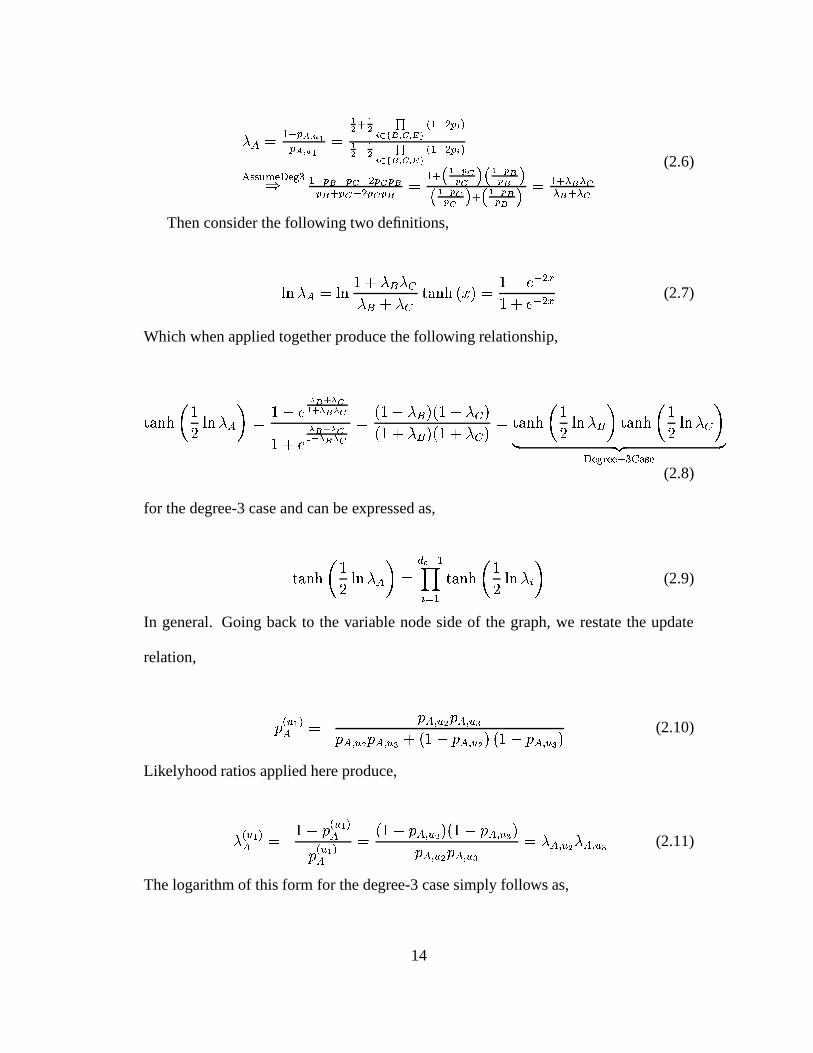
��� � # /�� ��� � �� ��� � � ����� �� ����� � ��� ��� � # / � � � ��� / �� ����� � ��� ��� � # / � � � �������� ��������� 1� # /�� /�� � / � � � � � � � � / � � � � � # �! �#"%$ �$ �'& �#"%$ $ & �#"($ �$ � & � �#"($ $ & � # � � � �� � � � (2.6)
Then consider the following two definitions,
)�* � � � )�* � � � � � �� �
� � �,+.- *0/ ����� � � �21 / �43� � 1 / �43 (2.7)
Which when applied together produce the following relationship,
+�- *0/65 ��)�* ���87 � � �91;: =< : �� < : : �
� � 1 : >< : �� < : : � �� � � � � � � � � � � �� � � � �
� � � � � � � � +�- *0/65 ��)�* � � 7 +.- *0/65 �
�)�* � �?7@ ACB D�����FE���� /21HG � �
(2.8)
for the degree-3 case and can be expressed as,
+�- *�/ 5 ��)�* ��� 7 � �HI / #�
9 � # +.- *0/ 5 ��)�* � 9 7 (2.9)
In general. Going back to the variable node side of the graph, we restate the update
relation,
�� ��� �� � ����� � � � ��� � �
����� � � ����� � � � � � � ����� � � � � � � ����� � � � (2.10)
Likelyhood ratios applied here produce,
�� ������ � � � �
� ��� ���� ������
�� � � ����� ��� � � � � ��� � ��� �
��� � � � ��� � � � � ����� ��� ����� ��� (2.11)
The logarithm of this form for the degree-3 case simply follows as,
14

)�* � � ��� �� � )�* � � � � � � )�* ����� � � (2.12)
and in general,
)�* � � ��� �� ���� / #�9 � # )�* � � � 9 (2.13)
2.2 The Approximate-Min*-BP technique
This section is presented in several parts. In the first part, our modified version
of Full-BP is introduced and its performance is contrasted to that of Full-BP. Next,
we provide a discussion of the steps taken in the derivation of this technique. At the
end of this section a complexity comparison between the proposed technique, Full-BP,
and a previously proposed reduced complexity technique [8] is provided. Section 2.3
gives a discussion of finite precision issues and provides performance data for several
quantization schemes. Section 2.4 describes the LDPC codec that has been developed
at UCLA based on the constraint update technique that is presented in the chapter.
Before describing the technique, we introduce notation that will be used in the re-
mainder of the chapter. On the variable node (left-hand) side of the bi-partite graph,
� messages arrive and�
messages depart. Both of these messages are log-likelihoods
(e.g.)�* � ) as described in the previous section. At the constraint node (right-hand)
side of the graph " messages arrive and � messages depart. All four message types
are actually log-likelihood ratios (LLRs). For instance, a message " arriving at a con-
straint node is actually a shorthand representation for " ��� ��
�� " �+� � � �
� " �#� ��� .15

The constraint node a-posteriori probability, or � � ��� , is defined as the constraint node
message determined by the � � variable messages that arrive at a constraint node of
degree- � � . The notation ��� � � � ��� � "�� denotes the outgoing constraint message de-
termined by all incoming edges with the exception of edge "�� . Message "�� represents
intrinsic information that is left purposefully absent in the extrinsic message compu-
tation ��� � � � ��� � "�� . Our algorithm (called Approximate-Min*-BP, or A-Min*-BP)
updates constraint messages as follows,
initialize
�" � �� � �� *� � #� � I � � "�� � � ��� � �����
for k =1 . . . � �
if� ������ � � �� � ���� � ��� � � � � / # � " � � ��
else:� � ��� � / #end� � ����� ���! " ��� � I� � ��� �#�� � ��� � � � � ����� ���! " � " � �� �$��% � ��� � � I�� � #!&(' * � "�� �
where � � is a storage variable, and � ��� � will be defined shortly. Constraint message
16

updates are found by applying the following additional operations on the above quanti-
ties.
���� � � #� �FI � � � �� � & ' * � "�� � & ' * � % � ��� � � � ���� � �� � & ' * � " �
�� � & ' * � % � ��� � � � ����� ���! "The above constraint node update equations are novel and will be described in fur-
ther detail. Variable node updating in our technique is the same as in the case of Full-BP.
Extrinsic information is similarly described as before via� � � � � ��� � � � , however the
processing required to achieve these quantities is much simpler,
� � ��� ����� � � � � � � �� � #� ��� � � � ��� � � �.� (2.14)
where � � is the variable node degree.
2.2.1 Derivation and complexity of the A-Min*-BP technique
Derivation of the Approximate-Min*-BP constraint node update begins with the so
called ‘Log-Hyperbolic-Tangent’ definition of BP constraint updating. In the equation
below, sign and magnitude are separable since the sign of LnTanh(x) is determined by
the sign of�
.
17

0.5 1 1.5 2 2.5 310
−8
10−7
10−6
10−5
10−4
10−3
10−2
10−1
100
Eb/N
o (dB)
BE
R
N=10k Irr A−Min*−BPN=10k Irr BP N=1k Irr A−Min*−BP N=1k Irr BP N=8k 3,6 A−Min*−BP N=8k 3,6 BP N=1k 3,6 A−Min*−BP N=1k 3,6 BP
Figure 2.3. A-Min*-BP decoding compared to Full-BP decoding for four dif-
ferent rate 1/2 LDPC codes. Length 10k irregular max left degree
20, length 1k irregular max left degree 9, length 8k regular (3,6),
length 1k regular (3,6). The proposed algorithm incurs negligible
performance loss. Note that rate 1/2 BPSK constrained capacity
is 0.18 dB ( � ����� ). All simulations were performed with the same
initial random seed.
� � ��� �� �FI�� � # & ' * � "�� ��� )�*������� � � 1 /�� I�� �� ���� � <�� " � � ��#" � " � � ����
� �21 / � I�� �� ����� <�� " � � ��#" � " � � � ��
������� � (2.15)
This equation is highly non-linear and warrants substantial simplification before
mapping to hardware. To begin, the above computation can be performed by first con-
sidering the inner recursion in (2.15),
18
� I� � � # )�* 5 � � 1%/�� � �� �21 /�� � � 7 � (2.16)
A total of � � table look-ups to the function ������� � )�* 5 # � � " � � �
# / � " � � � 7 followed by
� � � � additions complete the computation in (2.16). Furthermore, the linearity of
the inner recursion allows intrinsic variable values to be ‘backed-out’ of the total sum
before � � outer recursions are used to form the ��� extrinsic outputs. To summarize,
computation of all � � extrinsic values (in (2.15)) follow from ��� table look-ups, ��� � �
additions, � � subtractions, and a final � � table look-ups. The cost of computing the
extrinsic sign entails � � � � exclusive-or operations to form the � � � extrinsic sign,
followed by � � incremental exclusive-or operations to back-out the appropriate intrinsic
sign to form each final extrinsic sign.
Variable node computation (2.14) is more straightforward. However, a possible
alternative to (2.14) is given in [7] where it is noted that codes lacking low degree
variable nodes experience little performance loss due to the replacement of� � with
� � ��� . However, codes that maximize rate for a given noise variance in an AWGN
channel generally have a large fraction of degree-2 and degree-3 variable nodes [36].
Low degree nodes are substantially influenced by any edge input and� � ��� may differ
significantly from corresponding properly computed extrinsic values. We have found
experimentally that using� � ��� alone to decode capacity approaching codes degrades
performance by one dB of SNR or more.
We continue toward the definition of an alternative constraint update recursion by
rearranging (2.15) for the ��� � � case,
19

& ' * � " # � & ' * � " � � )�* 5 � � 1 � � � � � � � � �1 � � � � � 1 � � � � 7 � )�* 5 � � 1 � � � � �1 � � � 1 � � 7 � (2.17)
Two applications of the Jacobian logarithmic identity ()�* � 1 � � 1 � � - � � � � � � �)�* � � � 1 /�� � / � � ) [14] result in the Min* recursion that is discussed in the rest of the
chapter,
� ��� � � "$# � " � � � &(' * � " # � & ' * � " � � ��������� * � � "$# �$� � " � � �� )�* � � � 1%/ � � � � � � � � � � � �� )�* � � � 1 /�� � � � � /�� � � � � �
�������� � (2.18)
Note that (2.18) is not an approximation. It is easy to show that � � �,� recursions on
� ��� � yield exactly � � ��� in equation (2.15). Furthermore, the function)�* � � � 1 /�� 3 � �
ranges over�� �� � � ��� � which is substantially more manageable than the range of the
function ��� � ��� , � ����1 � )�* � # � � " ��# / � " ��� � � � � ��� � from a numerical representation
point of view. However, the non-linearity of the recursion (2.18) implies that updat-
ing all extrinsic information at a constraint node requires � ��� � � � � calls to � ��� � .
This rapidly becomes more complex than the � � � look-up operations (augmented with
� � � ��� additions) required to compute all extrinsic magnitudes based on the form in
(2.15). Again, in this earlier case intrinsic values can be ‘backed-out’ of a single � � �
value to produce extrinsic values.
Instead of using the recursion in (2.18) to implement Full-BP we propose that this
recursion be used to implement an approximate BP algorithm to be referred to as
Approximate-Min*-BP (A-Min*-BP). The algorithm works by computing the proper
extrinsic value for the minimum magnitude (least reliable) incoming constraint edge
20
0 1 2 3 4 5 6 7 8 9 100
0.1
0.2
0.3
0.4
0.5
0.6
0.7
x
y(x) = −0.25|x| + 0.6825 |x| < 2.8
y(x) = −0.375|x| + 0.6825 |x| < 1.0 = −0.1875|x| + 0.5 1.0 < |x| < 2.625
y(x) = ln(1 + e−|x|)
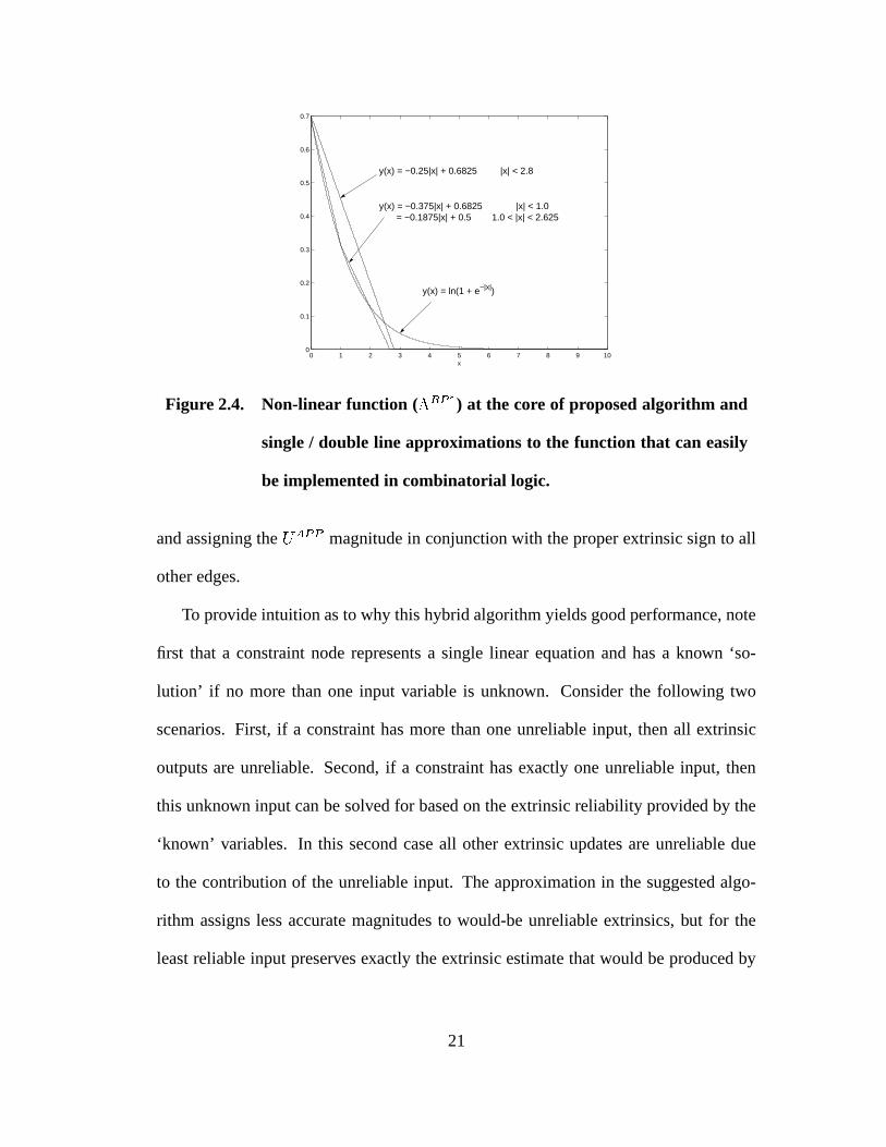
Figure 2.4. Non-linear function ( � ��� � ) at the core of proposed algorithm and
single / double line approximations to the function that can easily
be implemented in combinatorial logic.
and assigning the � � ��� magnitude in conjunction with the proper extrinsic sign to all
other edges.
To provide intuition as to why this hybrid algorithm yields good performance, note
first that a constraint node represents a single linear equation and has a known ‘so-
lution’ if no more than one input variable is unknown. Consider the following two
scenarios. First, if a constraint has more than one unreliable input, then all extrinsic
outputs are unreliable. Second, if a constraint has exactly one unreliable input, then
this unknown input can be solved for based on the extrinsic reliability provided by the
‘known’ variables. In this second case all other extrinsic updates are unreliable due
to the contribution of the unreliable input. The approximation in the suggested algo-
rithm assigns less accurate magnitudes to would-be unreliable extrinsics, but for the
least reliable input preserves exactly the extrinsic estimate that would be produced by
21

Full-BP.
We next show that � � ��� always underestimates extrinsics. Here the notation ��� �represents the extrinsic information that originates at constraint node � and excludes
information from variable node � . Rearrangement of (2.15) (with standard intrin-
sic/extrinsic notation included [9]) yields the following,
�� � � ��� �� � )�* � � ���� ��� � � �# / � " � ��� � �# � � " � � � � �
� � ���� ��� � � �# / � " � � �� � �# � � " � � �� � � (2.19)
� �21 / � � �� � �� � 1 /�� � �� � � � �� �
��� ��� � � � � � � �91%/�� � �� � �� � 1 /�� � � � �
�� 5 � �21%/�� � �� �� � 1 /�� � � � 7 � (2.20)
Note first that the function � ����� � # / � " ��# � � " �� (a product of which comprises the RHS
of (2.20)) ranges over� ��(� � and is non-decreasing in the magnitude of
�. The first
(parenthesized) term on the right-hand side of (2.20) equals the extrinsic value ��� �under the operator � ��� � , i.e. � � ��� � � . The second term scales this value by the intrinsic
reliability � � "�� � � . Hence, the monotonicity and range of � ����� ensure that �� � � ��� ����� ��� � � . We provide the inverse function, � / # ����� � )�* # � 3# / 3 , for reference.
Underestimation in A-Min*-BP is curtailed by the fact that the minimum reliabil-
ity � � " � �� � dominates the overall product that forms � � ��� . This term would have
also been included in the outgoing extrinsic calculations used by Full-BP for all but
the least reliable incoming edge. The outgoing reliability of the minimum incoming
edge incurs no degradation due to underestimation since the proper extrinsic value is
explicitly calculated. Outgoing messages to highly reliable incoming edges suffer lit-
tle from underestimation since their corresponding intrinsic � � "�� � � values are close to
22

Full-BP A-Min*-BP Offset-Min-BP
Table LookUps � � � � � � � 0
Comparisons 0 � � � � � � � �*�
Additions � � � � � 0 � �
XORs � � � � � � � � �"� � � � � �
Tot Table Lookups 80000 35000 0
Tot Comparisons 0 35000 65000
Tot Additions 75000 0 40000
Tot XORs 75000 75000 75000
Tot Ops 230,000 145,000 180,000
Performance Reference No Loss 0.1dB Loss
Table 2.1. Complexity comparison for three constraint update techniques.
Full-BP and A-Min*-BP have essentially the same performance.
The simplest technique, Offset-Min-BP, experiences about a 0.1dB
loss [7]. Numerical values are shown for a rate 1/2 code with:
� � � � �%����� , and average right degree ��� =8.
one. The worst case underestimation occurs when two edges ‘tie’ for the lowest level
of reliability. In this instance the dominant term in (2.20) is squared. An improved
version of A-Min*-BP would calculate exact extrinsics for the two smallest incoming
reliabilities. However, the results in Fig. 2.3, where the algorithm (using floating point
precision) is compared against Full-BP (using floating point precision) for short and
23

medium length regular and irregular codes, indicate that explicit extrinsic calculation
for only the minimum incoming edge is sufficient to yield performance that is essen-
tially indistinguishable from that of Full-BP.
The proposed algorithm is similar to the Offset-Min-BP algorithm of [8] where the
authors introduce a scaling factor to reduce the magnitude of extrinsic estimates pro-
duced by Min-BP. The Min-BP algorithm finds the magnitude of the two least reliable
edges arriving at a given constraint node (which requires � � � � comparisons followed
by an additional � � ��� comparisons). The magnitude of the least reliable edge is as-
signed to all edges except the edge from which the least reliable magnitude came (which
is assigned the second least reliable magnitude). For all outgoing edges, the proper ex-
trinsic sign is calculated. As explained in [9] these outgoing magnitudes overestimate
the proper extrinsic magnitudes because the constraint node update equation follows a
product rule (2.20) where each term lies in the range� ��(� � . The Min-BP approximation
omits all but one term in this product. To reduce the overestimation, an offset (or scaling
factor) is introduced to decrease the magnitude of outgoing reliabilities. The authors
in [8] use density evolution to optimize the offset for a given degree distribution and
SNR. The optimization is sensitive to degree sequence selection and also exhibits SNR
sensitivity to a lesser extent. Nevertheless, using optimized parameters, performance
within 0.1 dB of Full-BP performance is possible.
By way of comparison, A-Min*-BP improves performance over Min-BP because
the amount by which � � ��� underestimates a given extrinsic is less than the amount
by which Min-BP overestimates the same extrinsic. Specifically, the former underes-
timates due to the inclusion of one extra term in the constraint node product while the
24

latter overestimates due to the exclusion of all but one term in the product. A direct
comparison to Offset-Min-BP is more difficult. However, a simple observation is that
in comparison to Offset-Min-BP, A-Min*-BP is essentially ‘self-tuning’.
The range and shape of the non-linear portion ( � ��� � ) of the A-Min*-BP computa-
tion are well approximated using a single, or at most a 2-line, piecewise linear fit, as
shown in Fig. 2.4. All of the fixed precision numerical results to be presented in section
2.3 use the 2-line approximation (as do the floating point results in Fig. 2.3). Hence, the
entire constraint node update is implemented using only shift and add computations, no
look-ups to tables of non-linear function values are actually required.
The cost of constraint node updating for Full-BP (implemented using (2.15)), A-
Min*-BP, and Offset-Min-BP are given in Table 2.1. The latter two algorithms have
similar cost with the exception that ��� ��� table look-up operations in A-Min*-BP are
replaced with � � additions in Offset-Min-BP (for offset adjustment). Note that use of
a table is assumed for the representation of � � � ��� . While � ��� � is well approximated
using a two line piecewise fit employing power of 2 based coefficients. Variable node
updating occurs via (2.14) for all three algorithms.
2.3 Numerical Implementation
Minimum complexity implementation of the A-Min*-BP algorithm necessitates
simulation of finite wordlength effects on edge metric storage (which dominates de-
sign complexity). Quantization selection consists of determining a total number of bits
as well as the distribution of these bits between the integer and fractional parts (I,F) of
25

the numerical representation. The primary objective is minimization of the total num-
ber of bits with the constraint that only a small performance degradation in the waterfall
and error-floor BER regions is incurred. Quantization saturation levels ( � ��� � � � ) that
are too small cause the decoder to exhibit premature error-floor behavior. We have not
analytically characterized the mechanism by which this occurs. However, the following
provides a rule of thumb for the saturation level,
� ��� � � )�* ��� � )�* 5 � � �
�7 where � � 1 / � ��� �
This allows literal Log-Likelihood Ratio (LLR) representation of error probabilities
that are as small as � . In practice, this rule seems to allow the error-floor to extend to a
level that is about one order of magnitude lower than � .
In the results that follow, simple uniform quantization has been employed, where
the step size is given by �2/ � . To begin, Fig. 2.5 shows that low SNR performance
is less sensitive to quantization than high SNR performance. A small but noticeable
degradation occurs when 2 rather than 3 fractional bits are used to store edge metrics
and 4 integer bits are used in both cases. In summary, 7 bits of precision (Sign, 4 Integer,
2 Fractional) are adequate for the representation of observation and edge metric storage
in association with the considered code.
When power of 2 based quantization is used, the negative and positive satura-
tion levels follow � � � � / # � � � / # � �0/ � � . An alternative approach arbitrarily sets this
range between a maximum and a minimum threshold and sets the step size equal to
26
� � ��� � � � � � �=1 � � � � � � � 9 � , . This approach to quantization is more general than
the previous since the step size is not limited to powers of 2. We have found that in
the low SNR regime, smaller quantization ranges are adequate, but the optimal step
size remains similar to that needed at higher SNRs. Thus, operation at lower SNRs
requires fewer overall bits given the general range approach to quantization. For ex-
ample for ������� � ��� � dB, when� � � � � �=1�� �.� and a total of 6 bits were used,
no performance degradation was observed. For higher SNR values,� � � � ����1 �5�.�
was the best choice. This agrees with the results obtained using binary quantization
with� � ��� � � � � � � � . The performance of this quantizer is described in Fig. 2.5 by
the curve labeled ‘6bit G.R.’ (or 6 bit general range) where in this case the range is
set equal to (-10,10)@1.0dB;(-12,12)@1.2dB;(-16, 16)@1.4dB and a total of 6 bits (1
sign, 5 quant-bits) is used. Hence in this case the general range quantizer is equivalent
to the (1,4,1) power of 2 quantizer at high SNR. At lower SNRs, the best case range
was smaller than (-16,16) such that general range quantization offers an added degree
of freedom in precision allocation that is useful in the context of LDPC decoding.
2.4 The UCLA LDPC Codec
We have implemented the above constraint update technique along with many other
necessary functions in order to create a high throughput Monte Carlo simulation for
arbitrary LDPC codes. The design runs on a VirtexII evaluation board from Nallatech
systems and is interfaced to a PC via a JAVA API. A block diagram is provided in
Fig. 2.6. The Gaussian noise generator developed by the authors in [13] is instantiated
27

0 10 20 30 40 50 60 70 8010
−9
10−8
10−7
10−6
10−5
10−4
10−3
10−2
10−1
100
Iterations
BE
R
Eb/N
o=1.0 dB
Eb/N
o=1.2 dB
Eb/N
o=1.4 dB
8bit=(1,4,3)7bit=(1,4,2) 6bit G.RFull Prec.
(a)
1 1.1 1.2 1.3 1.4 1.5 1.610
−8
10−7
10−6
10−5
10−4
10−3
10−2
10−1
Eb/N
o (dB)
BE
R
20 Iterations
30 Iterations
70 Iterations
8bit=(1,4,3)7bit=(1,4,2)6bit G.RFull Prec
(b)
Figure 2.5. (a) BER Vs. � ����� , for different fixed numbers of iterations. (b)
BER vs Iterations, for different fixed � ����� .
next to the decoder so as to avoid a noise generation bottleneck. This block directly im-
pacts the overall value of the system as a Monte Carlo simulator for error-floor testing
as good noise quality at high SNR (tails of the Gaussian) is essential. Since the LDPC
decoding process is iterative and the number of required iterations is non-deterministic,
28

����������� ���������������������������� �"!�#$�%���
&'()*+,-./0
1234452+6-54/1/+
78-9)-+:0-8;3<</0
=:/02:5>/'/,-./0
?�@BADC�EGFIH
J HGKL@BF MONPFIF @BFIQ
R EGS ET�@BU�FVKLH?�@BM�H R HGW ?�@BM�H R HGWT�X J
Figure 2.6. Architecture block diagram.
a flow control buffer can be used to greatly increase the throughput of the overall sys-
tem.
Through the use of JAVA as an soft interface to the board, we have been able to fa-
cilitate the initiation and monitoring of simulations from remote locations. Researchers
around the world have successfully uploaded their own LDPC codes for testing on the
“UCLA Monte Carlo System”.
2.5 Conclusion
A reduced complexity decoding algorithm that suffers little or no performance
loss has been developed and is justified both theoretically and experimentally. Finite
wordlengths have been carefully considered and 6 to 7 bits of precision have been
shown to be adequate for a highly complex (a length 10,000 � � � � 3 � ��� irregular
29

LDPC) code to achieve an error floor that is code rather than implementation limited.
30

Chapter 3
Parity Check Matrix Construction for
Error Floor Reduction
Density evolution determines the performance threshold for infinitely long codes
whose associated bipartite graphs are assumed to follow a tree-like structure. How-
ever, bipartite graphs representing finite-length codes without singly connected nodes
inevitably have cycles and thus are non-tree-like. Cycles in bipartite graphs compro-
mise the optimality of the commonly practiced belief propagation decoding. If cycles
exist, neighbors of a node are not conditionally independent in general, therefore graph
separation is inaccurate and so is Pearl’s polytree algorithm [34] (which defines belief
propagation as a special case). However, not all cycles are equally problematic in prac-
tice. We will argue that the more connected a cycle is to the rest of the graph, the less
difficulty it poses to iterative decoding.
Randomly realized finite-length irregular LDPC codes with block sizes on the order
31

of �.� � [36] approach their density evolution threshold closely (within 0.8dB at BER
� �.�0/ � ) at rate � � � , outperforming their regular counterparts [29] by about 0.6dB.
In this work, we repeated the irregular code construction method described in [36] and
extended their simulation to a higher SNR region. In the relatively unconditioned codes,
an error floor was observed at BERs of slightly below �.� / � . In contrast, regular codes
and almost regular codes ([24]) usually enjoy very low error floors, apparently due
to their more uniform Hamming distance between neighboring codewords and higher
minimum distances.
MacKay et al. [29] first reported the tradeoff between the threshold SNR and the
error floor BER for irregular LDPC codes versus regular LDPC codes. A similar trade-
off has been found for turbo codes ([3], [16]). This work presents a design technique
that requires all small cycles to have a minimum degree of connectivity with the rest of
the graph. This technique lowers the error floors of irregular LDPC codes significantly
while only slightly degrading the performance in the waterfall region.
The error floor of an LDPC code under maximum likelihood (ML) decoding de-
pends on the � � 9 � of the code and the multiplicity of � � 9 � error events. However, for
randomly constructed codes, no algorithm is known to check if they have large mini-
mum distances (This problem was proved to be NP-hard [47]).
As a result, the common approach has been to indirectly improve � � 9 � through
code conditioning techniques such as the removal of short cycles (girth conditioning
[31], [2]). Such conditioning is useful also because certain short cycles can cause poor
performance in conjunction with iterative decoding even if they have a large ��� 9 � and
would not be problematic for ML decoding.
32

However, not all short cycles are equally harmful. Standard girth conditioning
severely constrains code structure by removing all cycles shorter than a specified length
even though many of these can do little harm, because they are well-connected with the
rest of the graph. This work uses a technique precludes only cycles that are relatively
isolated from the rest of the graph and thereby are likely contributors to small stopping
sets. Di et al. [12] described stopping sets in the context of erasures. Message passing
decoding fails whenever all the variable nodes in a stopping set are erased. Notably,
erasing all variable nodes in a stopping set does not necessarily force ML decoding to
fail.
For QPSK and BPSK modulation, Euclidean distance and Hamming distance are
linearly related. Thus, it is reasonable to design codes for such modulations to focus on
the Hamming distance spectrum. Minimum Hamming distance ( � � 9 � ) is well-known
to be related to the number of errors ( � ) that can be corrected reliably, � � 9 � � � � � � .Minimum Hamming distance is also known to be linearly related to the number of
erasures ( � ) that can be corrected, � � 9 � � � � � . As we will show, the minimum
stopping set size is equal to the smallest number of erasures that cannot be corrected
by iterative decoding. Thus it is closely related to the Hamming distance (and hence
Euclidean distance for QPSK and BPSK). Because the weight distribution of stopping
sets is so closely related to the Euclidean distance spectrum, it is clear that LDPC
designs focusing on the weight distribution of stopping sets is appropriate for AWGN
channels as well as the binary erasure channel (BEC).
The focus of this work is on LDPC codes for AWGN channels, but we improve
erasure performance (stopping set size) to indirectly improve AWGN performance. As
33

demonstrated by our simulations, we can reduce error floors in AWGN channels by
generating codes from an expurgated ensemble that has large stopping sets. The result-
ing codes outperform the girth-conditioned irregular codes described in [31] and [2].
The work is organized as follows. Section 3.1 shows the relationship between cycles,
stopping sets, and codewords. Section 3.2 proposes a design metric termed extrinsic
message degree (EMD). Based on the approximate cycle EMD (ACE), section 3.3 de-
scribes a linear-time Viterbi-like algorithm to construct full-rank parity-check matrices
that follow irregular degree distributions but do not have isolated small cycles. This
indirectly forces a large stopping set size. Section 3.4 demonstrates by simulation the
substantial decrease in error floor achieved by ACE-conditioned codes as compared to
girth-conditioned codes.
3.1 Cycles, stopping sets, codeword sets and edge-expanding
sets
The well known matrix and bipartite graph descriptions of a rate 1/3� ���� � code are
given in Fig. 3.1. This code will be used in examples throughout the chapter. One
column in the parity-check matrix corresponds to one variable in the bipartite graph.
For convenience, we will use ‘column’ and ‘variable’ interchangeably in this chapter.
The parity-check matrix % is constructed such that its % � portion is invertible, which
guarantees that % is full-rank. For systematic encoding, % # corresponds to information
bits and % � corresponds to parity bits.
34

��������
�
�
��������
�
�
������
������
������
������
������
������
������
������
������
� � variable nodes
constraint nodes
+
+
+
+
+
+
message nodes
check nodes
� � � � � � � � � � � � � � � � �� � � � �� �� �� �
� � � � �� �� �� �
��� � � ����� �� ����� �� �
(a) (b)
H =
Figure 3.1. Matrix and graph description of a (9, 3) code.
3.1.1 Cycle-related structures
Definition 1 (Cycle) A cycle of length � � is a set of � variable nodes and � constraint
nodes connected by edges such that a path exists that travels through every node in the
set and connects each node to itself without traversing an edge twice.
Definition 2 ( � � Cycle set) A set of variable nodes in a bipartite graph is a ��� set if
(1) it has � elements, and (2) one or more cycles are formed between this set and its
neighboring constraint set. A set of � variable nodes does not form a ��� set only if no
cycles exist between these variables and their constraint neighbors.
Note that the maximum cycle length that is possible in a ��� set is � � . Fig. 3.1 shows
a length-6 cycle ( "�� ��� � � " � ��� # � " � ��� 6 � "%� ) and a length-4 cycle ( " � ��� # � " � ��� 1 � " � ).Variable node set 7 "��.� " � � " � 8 is a � 1 set. Variable node set 7 " � � " 6 � " � 8 is also a � 1 set
35

although " 6 is not contained in the length-4 cycle. Di et al. defined a stopping set as
follows, which we will show to contain cycles shortly.
Definition 3 ( � � Stopping set [12]) A variable node set is called an � � set if it has �
elements and all its neighbors are connected to it at least twice.
Variable node set 7 "��)� " � � " � 8 in Fig. 3.1 is an � 1 set because all its neighbors �(� , � # ,� 1 and � 6 are connected to this set at least twice.
The following lemma shows that stopping sets always contain cycles. The effec-
tiveness of message passing decoding on graphs with cycles depends primarily on how
cycles are clustered to form stopping sets.
Lemma 1 In a bipartite graph without singly connected variable nodes (such as one
generated with a degree distribution given by density evolution), every stopping set
contains cycles.
Proof: A stopping set (variable nodes) and its neighbors (constraint nodes) form
a bipartite graph where one can always leave a node on a different edge than used to
enter that node. Traversing the resulting bipartite graph in this way indefinitely, one
eventually visits a node twice, thus forming a cycle.�
Lemma 2 In a bipartite graph without singly connected variable nodes, stopping sets
in general are comprised of multiple cycles. The only stopping sets formed by a single
cycle are those that consist of all degree-2 variable nodes.
Proof: A cycle that consists of all degree-2 variable nodes is a stopping set. To prove
the lemma, we only need to show that if a cycle contains variable nodes of degree-3 or
36

more, any stopping sets including this cycle are comprised of multiple cycles. Fig.
3.2(a) shows a cycle of arbitrary length � � (here � � �� for demonstration). Assume
that one variable node " � in this cycle has degree 3 or higher, " � must be connected
to at least one constraint node out of this cycle (for instance � # in Fig. 3.2(a)). By
the definition of a stopping set, � # must be connected to variable nodes in the stopping
set at least twice. Therefore if ��# is not connected to " # , or " 1 , or " � , the stopping set
must contain at least one more variable node (for instance " 6 ). The ‘concatenation’ of
constraints and variables on to " 6 may occur across many nodes. However, to form a
stopping set, eventually a new loop must be closed that connects the newest constraint
in the chain to a variable on the chain or in the original cycle. Thus, the stopping set is
comprised of at least two cycles.�
+
+
+
+ v4
v3
v2 v1
(a) (b)
+
v5
extrinsic component of v2
c1
Figure 3.2. (a) Extrinsic message (b) Expanding of a graph
According to Lemma 2, the general view of stopping sets and cycles is given in
Fig. 3.2(b). Two types of variable nodes comprise a stopping set. Variable nodes of the
37

first type form cycles with other variable nodes; variable nodes of the second type form
binding structures that connect different cycles. It should be noted that both binding
nodes and cycle nodes may have branches that lead to cycles containing variable nodes
not in the current stopping set. Our proposed parity matrix design algorithm ensure that
short cycles contain at least a given minimum number of ‘extrinsic paths’. This leads
to an increase in the minimum size of a stopping set.
Definition 4 ( !� Codeword set) A variable node set is called a � set if it is com-
prised of exactly � elements whose columns form a (weight-d) codeword.
Variable nodes set 7 "%�(� " � � " � 8 in Fig. 3.1 is the 1 set corresponding to the code-
word 100010100. A linear code with minimum distance � � 9 � has at least one codeword
with weight � � 9 � and no non-zero codewords with smaller weight. Hence, there is at
least one !� � � set but no !� sets where � � � � 9�.
Erasing all the variables in a codeword set is the same as erasing all the non-zero
positions of a binary codeword. Recovery from such an erasure is impossible even
under ML decoding. Thus all codeword sets are stopping sets.
Preventing small stopping sets also prevents small � � 9 � . If a code has � � 9 � , it must
have an ��� � � stopping set. Thus, avoiding all stopping sets � � for ��� � ensures
� � 9 ��� � .
However, small stopping sets do not necessarily represent low distance events. In-
deed, an ML decoder can successfully decode an erased stopping set if a full column-
rank sub-matrix is formed by the columns of the parity check matrix that are indexed by
the stopping set variables. For example, 7 " 1 � " � � " 6 � " � � "��)8 in Fig. 3.1 is a stopping set
38

that may be recovered by ML decoding (in the BEC case, simply solve a linear equation
set). However, an erased stopping set can never be overcome by an iterative decoder.
With additive white Gaussian noise (AWGN), the magnitude of a corrupted signal
can be so small that it can be effectively treated as an erasure. Hence the role of stop-
ping sets can be translated to AWGN scenarios where variables with poor observation
reliability are analogous to erasures. All stopping sets of small size are problematic.
Some cause small distance, and all cause problems for iterative decoding. An obvi-
ous direction to take in order to generate codes well-suited to iterative decoding is to
increase the size of minimum stopping set and reduce its multiplicity. Fig. 3.3 summa-
rizes the relationship between � � , � � , and !� . Here, �� is a graph structure that we
will discuss in the next section.
{Cd}
{Sd}
{Wd}
{Ed}
Figure 3.3. Venn diagram showing relationship of ��� , � � , !� and �� .
39

3.1.2 Cycle-free sets
At this point, the value of removing small stopping sets is apparent. However, one
might argue that simple girth conditioning accomplishes this because every stopping
set contains cycles. The problem with traditional girth conditioning is that there are so
many cycles. Fig. 3.4 illustrates a cycle in the support tree of variable node "0� of Fig.
3.1. All the levels whose indices are odd numbers consist of constraint nodes and all
the levels whose indices are even numbers consist of variable nodes. A cycle occurs
if two positions in the support tree represent the same node in the bipartite graph (e.g.,
"�� in level-3). To detect cycles of length up to � � in the support tree of "�� , we need to
expand its support tree � levels.
+ +
v0
c0 c5
v2 v4 v8 v1 v6 v7 v8
Level-0
Level-1
Level-2
Figure 3.4. Traditional girth conditioning removes too many cycles.
The number of nodes in the support tree grows exponentially with the number of
levels expanded. To be short-cycle-free, all these nodes have to be different, so the
longest cycle size we can avoid increases only logarithmically with block size (see
[18]). Since the logarithm is a slowly increasing function, girth conditioning of a finite
length LDPC code is severely limited by block length.
40

Girth conditioning is especially problematic when there are high-degree nodes, as
is common with degree distributions produced by density evolution. Recent girth con-
ditioning techniques usually bypass high degree nodes. For example, in [31], the edge-
wise highest variable degree is only 3; in [2], the fraction of the highest degree variables
� � is only 0.025. As a result, girth conditioning was easier to perform. However, the
capacity-approaching capability was sacrificed. High degree nodes are indicated by
density evolution and lead to large stopping sets. The following arguments further dis-
cuss the cycle-related structures for high degree nodes and low degree nodes.
Definition 5 (Cycle-free set) A variable node set is called a cycle-free set if no cycle
exists among its constituent variables.
Theorem 1 A necessary and sufficient condition for a set of degree- � variable nodes
to be a cycle-free set is that this set is linearly independent.
Proof: All sets that are not linearly independent contain codeword sets. Codeword
sets are special stopping sets and stopping sets contain cycles (Lemma 1). For suffi-
ciency, note that the constraint nodes taking part in a cycle among degree-2 nodes are
each shared by exactly two variable nodes. Therefore the binary sum of columns (vari-
ables) taking place in the cycle is the all-zero vector and these columns are linearly
dependent.�
Corollary 1.1 A maximum of ��� � �'� degree-2 columns of length � � � may be
linearly independent (cycle-free).
Proof: Consider the�� � �
���� � � �"� � bi-diagonal matrix,
41
����������������������
� � ����� �
� �
� � . . .
.... . .
� �
� �
� ����� � �
�����������������������
�/�� / #
�/�� � (3.1)
This matrix forms a rank � � � � � basis of degree-2 columns each with dimension
� � � . Any possible degree-2 column of dimension � � � can be formed via a linear
combination of columns in the above basis.�
Corollary 1.1 may also be considered a version of the Singleton bound where the
restriction to degree-2 columns lowers the best possible � � 9 � from � � � to � � � �"� .
Theorem 2 In an ( � ,�
) code free of degree-1 variables, a cycle-free variable node set
" # � " �)�(� � � � " , must satisfy ,9 � # � ��9 � � � � � � � �"� , where ��9 is the degree of " 9 .
Proof: A degree- � variable node whose constraints are 7 � # � � �(�)� � � � � �(8 can be con-
ceptually replaced by a cluster of � �"� degree-2 nodes whose constraints are 7 � # � � �)8 ,7 � �(� � 1 8 , ..., 7 � � / # � � �(8 respectively. As an example, Fig. 3.5 shows how variable node
" # in Fig. 3.1 may be replaced by a cluster of two degree-2 nodes.
Because the indices of the constraints in a cluster are ordered, any cycle involving
the degree- � node is equivalent to a cycle involving some of the degree-2 nodes in the
cluster replacing the original node. Fig. 3.6 shows an example. Replace every variable
42

5
4
3
2
1
0
...
...
...
...
...
...
1
1
0
0
1
0
c
c
c
c
c
c
��������
�
�
��������
�
�
)c ,(c)c ,(c1
1
0
0
0
0
0
1
0
0
1
0
5441
��������
�
�
�
��������
�
�
�
variable node v1:
cluster of degree-2 nodes:
Figure 3.5. "$# can be replaced by two degree-2 nodes.
in the set with its equivalent cluster. According to Corollary 1.1, at most � � � � � of
these resulting degree-2 nodes can form a cycle-free set. Thus the theorem is proved.�
Corollary 2.1 In an ( � ,�
) code free of degree-1 variables, no set of variable nodes
whose cardinality is larger than � � � � � can be cycle-free.
Proof: Equality in the inequality of Theorem 2 is achieved with � � � � � indepen-
dent degree-2 variable nodes. Fewer variable nodes are allowed if some have higher
degree.�
Lemma 2 and Theorem 1 show that for degree-2 variable nodes, cycles, stopping
sets and codeword sets are equivalent. These structures are distinct for higher degree
nodes following the Venn diagram of Fig. 3.3. Theorem 2 shows that higher degree
nodes may be considered as the superposition of two or more degree-2 nodes, and they
tend to form cycles more easily. As a result, girth conditioning on high degree nodes
is more difficult than on low degree nodes. However, cycles involving higher degree
nodes are actually less problematic because they have higher EMD, as will be explained
in the next section.
43

�
�
�
�
�
�
�
�
�
�
�
�
�
�
�
�
�
�
� �
� �
� �
�
�
�
�
�
�
�
�
�
�
�
�
�
�
�
�
�
�
� �
� ���
�
�
�
�
�
�
� ���
� ���
�
�
�
�
�
�
� ���
(a) (b)
Figure 3.6. Replace "$# by its cluster in a cycle.
3.2 EMD and LDPC code design
Our goal is to ensure that all stopping sets have at least some minimum number of
variable nodes. However, no polynomial-time algorithm is known that removes small
stopping sets explicitly, and our attempts to directly control stopping set sizes were too
complex even to prevent very small stopping sets in a reasonable amount of time. As
an alternative, we design an algorithm that conditions the graph so that small cycles all
have an edge expanding property that prevents them from being part of a small stopping
set. First, we define the notion of an edge expander as presented in [12].
Definition 6 (( , ) edge expander [12]) Let � be any subset of left nodes (variable
nodes). Define � � � to be the number of edges connected to � and � ���
to be the
number of neighbors of � . An ( , ) edge expander of an ( � ,�
) code is a graph that
has � ��� � �
��
for all subsets with ��� �� � .
44

Methods that realize regular graphs with good edge expanding properties were pro-
posed by Margulis in [32]. However, a construction that can simultaneously satisfy a
given edge expanding property as well as a given irregular degree distribution has yet
to be proposed. We are interested in the special case of� �(� � � � edge expanders.
Definition 7 ( �� Edge-expanding set with parameter *� � � � ) A set of � variable
nodes is called an �� set if one-half of the number of edges emanating from it is less
than the number of neighbors to which these edges connect.
Neighbors (constraints) of an �� set are connected to the set less than twice on
average, therefore at least one neighbor exists that is singly connected to this � set.
Thus, as shown in Fig. 3.3, the set of � � sets and the set of �� sets are disjoint. For
a given value of � , increasing the number of �� sets decreases the number of possible
� � sets. Hence, conditioning for good edge expansion indirectly reduces the number of
small stopping sets.
Lemma 2 shows that stopping sets are comprised of linked cycles. An efficient way
to suppress small stopping sets is to improve the edge expanding properties of cycles
in an irregular LDPC code. From the discussion of �� sets, we know that constraint
nodes singly connected to a variable node set provide good edge expansion because
these constraint nodes ensure useful message flows. Our algorithm achieves this by
focusing on a parameter of variable node sets that we call the extrinsic message degree
(EMD).
Definition 8 (Extrinsic message degree) An extrinsic constraint node of a variable
node set is a constraint node that is singly connected to this set. The extrinsic message
45

degree (EMD) of a variable node set is the number of extrinsic constraint nodes of this
variable node set.
As was previously described, the high-SNR performance of an iteratively decoded
LDPC code is limited by the size of the smallest stopping set in the code. The EMD of
a stopping set is zero. A set of variable nodes with large EMD will require additional
concatenation of nodes to become a stopping set. We propose a conditioning algorithm
that ensures all cycles less than a given length have an EMD greater than a given value.
This technique statistically increases the smallest stopping set size. It also increases
� � 9 � because codeword sets are special cases of stopping sets.
The algorithm that follows ignores large cycles. In the context of EMD, this is
justified for two reasons. First, large cycles necessarily contain many variable nodes.
Second, they tend toward high EMD by virtue of a level of graph connectivity that
statistically surpasses that of small cycles. We thus target the elimination of small
cycles with low EMD and claim (via the arguments of previous sections) that these
structures are significant contributors to errors at high SNR.
3.3 Construction of LDPC codes free of small stopping
sets
First consider the EMD of a generic cycle. If there are no variable nodes in a cycle
that share common constraint nodes outside of the cycle, then the EMD of this cycle
is 9 � ��9 � � � , where ��9 is the degree of the � ��� variable in this cycle. Otherwise, the
46

EMD is reduced through constraint node sharing. To provide a calculable EMD metric,
we neglect constraint node sharing and define an approximate cycle EMD.
Definition 9 (Approximate cycle EMD (ACE)) The ACE of a length � � cycle is 9 � ��9 � � � ,where ��9 is the degree of the � ��� variable in this cycle. We also say that the ACE of a
degree- � variable node is � � � and the ACE of any constraint node is 0.
ACE is an upper bound on EMD. The code conditioning algorithm to be proposed
next is based on ACE instead of EMD. This approximation is reasonable since in this
algorithm, all cycles shorter than a given length (including those formed through con-
straint node sharing) will be required to meet the ACE criteria. An LDPC code has
property ( �$���� , � ����� ), if all the cycles whose length is � � ���� or less have ACE values
of at least � ����� .In our codes information bits come before parity bits (see Fig. 3.1). We assign
column nodes such that degree decreases monotonically (i.e., � 9 � � � if � � �). Be-
cause high degree nodes converge faster, this arrangement provides more protection to
information bits than to parity bits. The algorithm is as follows:
47

for ( � � � �"� ; � � � ; � � � )
begin
redo:
Randomly generate "%9 according to deg. distr.;
if � � �(i.e., " 9 is a parity bit)
begin
Gaussian Elimination (GE) on % � ;
if " 9��!� � � � � " �9 � # � " �9 � � �(� � � � " �� / #�
goto redo;
else
" �9�� the residue of " 9 after GE;
end
ACE detection for " 9 ;if � �� � � ����� for a cycle of length � �$����� or less
goto redo;
end
The Gaussian elimination process ultimately guarantees that the H matrix has full
rank by ensuring that the � � � columns of % � will be linearly independent. For degree-
2 variable nodes, independence entails freedom from cycles so that all degree-2 parity
check nodes will be cycle-free. A caveat is that if Gaussian elimination is used in
conjunction with a degree distribution that yields more than � � � degree-2 nodes, then
at least one of the � � � parity check variables should have odd number degree (this
48

can be achieved by column swapping). This follows immediately from Corollary 1.1.
The ACE detection method can be equivalently depicted in two ways. The first one,
based on support trees, is directly related to the graph structure. The second one, based
on trellises, is oriented for algorithm implementation.
The tree depiction of ACE detection ( � �����,� � ) is given in Fig. 3.7. Here, variable
and constraint node labels refer literally to those of the example code in Fig. 3.1 and
the support tree that extends four levels below root node "�� is portrayed. We define � �
to be the ACE of a path between root node "�� and an arbitrary node � � (it can be either
a variable node or a constraint node). Recall also that � �� � � � � � � 1 ��� 1 1 � � � � � � if
� � is a variable, and � �� � � � � � � if � � is a constraint.
49

ACE Detection of "%�
� � � � for all variables and constraints;
��� � � �� � " � � ; Activate "%� for level-0;
for ( � � � ; � � � ����� ; � � �)
begin
for any active node � , in level-( � � � )
begin
Find its children set � � � � , � ;for every child � � � � � � � , �begin
� � � � � � ��� , � � � �� � � � � ;
if�
� � � � � � � � � ���� � " � � � � �� � � � ��� � � ����� 1
exit with failure;
elseif � � � � � �� �
Deactivate � � in level- � ;
else
� � � � � � � � ;end
end
end
exit with success;
�Note that if ������� ������������������������� �!���"��#$�%�&�('*) , this is the ACE of a cycle involving #+� .
50

To explain the above algorithm, we need to recognize that a node should propagate
descendants (be active) only if the path leading to this node has the lowest ACE value
that any path to this node has had thus far. Therefore linear cost is achieved instead
of an exponential cost. Initially all the path ACEs can be set to � (which means
‘unvisited’). Note that cycles occur when a node is revisited, is simultaneously visited,
or both. A cycle ACE equals the sum of the previously lowest path ACE to a node
and the current path ACE to the node minus the doubly counted root and child ACE.
When a cycle is formed by connecting two distinct paths from "�� to � � we have cycle
� �� � � � � � � � � � � ���� � " � � � � �� � � � � , where � � � � � and � � are the ACEs of the
two paths from "%� to � � . Handling multiple simultaneous arrivals to the same node is a
trivial extension where ACE minimization is performed sequentially across all arrivals.
In the example shown in Fig. 3.7, bold lines at each level describe the current set of
active paths. In this example ‘ties’ are assigned the path whose parent has the lowest
index. For instance the path ( "�� - � 6 - " # - � # ) with � �� �#� survives while, ( "�� - � 6 - " � -� # ), ( " � - � � - " � - � # ), ( " � - � � - " � - � # ) each also having ������ , perish. For an example of
pruning occurring due to cycle detection on differing levels of the tree, observe that the
path ( "%� - � � - " � - � 6 ) with � ��� � does not survive since � 6 was visited at Level-1 and
was accordingly assigned ���� � � .Fig. 3.8 provides a trellis depiction of the previous discussion (with two more stages
added). A trellis instead of a full support tree is adequate for ACE detection because the
ACE minimization is performed sequentially and only the minimum ACE needs to be
stored. Again, a path ACE is stored for every variable node and every constraint node.
An active path is a path that connects the root variable node and any other node with
51

0 1 2 3 4 5 6 7 81 1 1 1 020 1 1ACE
1 54 6 3 58 1 256 36 7 1 235 10 671
5
4 1 3 4 5 4 1 3
456 2358 1 22 45 3 4 7 3 4 6 0 1 23 5
1 76 8842
0
0
1 3 0 4
42
1
V
0
1 1 0 1
1000111010111
1 1 1
0 0
V V
C
C
V VV VVVV
C
V
C C C C C C C C C C CC
V V
Figure 3.7. Illustration of an ACE search tree associated with "�� in the exam-
ple code of Fig.3.1. � �������� . Bold lines represent survivor paths.
ACE values are indicated on the interior of circles (variables) or
squares (constraints), except on the lowest level where they are in-
stead described with a table.
the lowest ACE value up to the current step. Active paths are marked by solid lines in
Fig. 3.8. An active node is a node that connects to an active path at the current step.
Viterbi tree pruning yields a complexity at each root that is upper bounded by
� ����� � � ��� ��� � where � is the highest degree of any node in the graph, because
the support tree is expanded � ����� levels, for each level we have to consider at most
� nodes, and every node has at most � � � children. As shown in Fig. 3.8, relatively
few nodes at a level are active, thus the actual computational burden is reasonable, even
for block size on the order of �.��6 bits. The storage space needed is on the order of
� � �� � �
�because only the current trellis level has to be saved. To further improve
run-time, any active node with path ACE � �� � ����� can be deactivated because all
the paths stemming from this node have an ACE value of at least �$����� . As a special
52

v0
v1
v2
v3
v4
v5
v6
v7
v8
c0
c1
c2
c3
c4
c5
0 0
0
1
1
0
1
1
0
1
0
1
0
1
0
0
1
1
1
1
2
1
0
1
0
1
1
0
0
1
0
1
1
1
1
2
1
0
1
+
+
+
+
+
+
+
+
+
+
+
+
+
+
+
+
+
+
Figure 3.8. The Viterbi-like ACE algorithm. � ����� ���
application of this argument, the user may generate columns for all variable nodes with
degree � ���� � � or higher without checking the ACE (since all descendants will have
a path ACE of at least � ����� ).Note that cycle detection can be implicitly performed in the above algorithm. Un-
visited variables are initialized to � � � � . When a variable is first visited, � � is assigned
a finite value. Upon subsequent visits to the same variable, ill-conditioned cycle detec-
tion is alarmed if the condition�
� � � � � �� � � � �� � " � � � ���� � � � ��� � � ����� is not
satisfied.
3.4 Simulation results and data analysis
We present results for LDPC codes with three different block lengths.
53

3.4.1 Block-length 10,000 LDPC codes
We used the ACE algorithm to construct (10000, 5000) codes that have the irregular
degree distribution given in [36] with maximum variable node degree � �&� �%� . The
encoded bits were sent through a binary-input AWGN channel. For each corrupted
codeword, a maximum of 200 iterations were performed. Each simulation was stopped
when 80 block errors were detected. The BER results and in one case the word (block)
error rate (WER) results are plotted in Fig. 3.9.
A ( � ����� , � ���� ) code in Fig. 3.9 means that in this code, all cycles of length up
to � � ����� have ACE of at least � ����� . Higher � ����� values ensure better properties
for the conditioned cycles and higher � ���� values ensure that conditioning occurs for
longer cycles. There is a tradeoff between � ����� and � ����� : increasing one param-
eter inevitably makes the other parameter more difficult to implement. For � ����� ��.��)�.�� �� � � and � , the highest � ����� values that we could achieve were � ���� � � � , and �
respectively. If all degree-2 variables are parity bits (which is possible if there are fewer
than � � � of them), then the full-rankness of the parity matrix guarantees that no cycles
will exist between degree-2 variables (see Theorem 1). In this case we can construct
( � , 1) codes since all cycles of any length must include nodes of at least degree-3 (and
hence have ACE of at least 1). Such codes have the lowest level of conditioning that
we consider and we use codes constructed in this manner to contrast the performance
of stronger ( �$���� , � ���� ) conditioning levels.
As a benchmark, Richardson and Urbanke’s �.� � -bit code [36] (referred to here as
the RU code) is included in Fig. 3.9(a). This RU code was constructed with the con-
54

straint that “all the degree-two nodes were made loop-free”. Unfortunately, simulation
results below BER �.�2/ � are unavailable for the RU code. The ( � , 1) code shown
in this chapter has a similar level of conditioning as the RU code and exhibit compa-
rable performance. The ( � , 1) code ensures linear independence among parity bits
which include all degree-two nodes and some degree-three nodes. The error-floor BER
of the ( � , 1) code is around �.� / � . Pure length-4 cycle removal improves BER by
half an order in magnitude over the ( � , 1) code at highest SNR, and adversely affects
convergence. However, proper selection of � ����� and � ���� suppresses error floors
significantly more. For example, the pure ACE conditioning code (9, 4) achieves ap-
proximately BER = �.� /�� , three orders of magnitude below the ( � , 1) code.
Fig. 3.9(b) compares several ACE parameter sets with or without explicit length-4
cycle removal. Note that the lowest error floor was achieved at � �����,��� and � ����� � �
with no explicit removal of short cycles. As explained before, traditional girth con-
ditioning treats all short cycles equally, thus making the removal of longer but still
harmful cycles more difficult. On the contrary, the ACE algorithm effectively removes
low-ACE cycles, while leaving shorter cycles intact, if they have a high ACE. By doing
this, participation of high degree variables in cycles is encouraged. In fact, removing
all length-4 cycles hinders the performance of the ACE algorithm.
We observe that there is a small penalty in the capacity-approaching capability of
our low-error-floor codes. With more conditioning at this block size, the low-SNR
performance of the code is slightly degraded, possibly due to a decrease in the random-
ness of the code structure. This tradeoff between error floor and low-SNR performance
is a well-known characteristic of iteratively decoded codes ([29][3][16]). Scheme (9,
55

4) is approximately 0.07dB away from the RU code at low SNR. However, even with
this mild penalty these codes remain superior to regular codes in terms of their capacity-
approaching performance. For example, we tested MacKay’s (9972, 3, 6) regular LDPC
code described in [29]. Although no error floors were detected for this code, it achieves
����� � �.� /26 at � �, � ��� � dB, more than 0.6dB worse than our (9, 4) code. Thus the
combination of density evolution optimized degree distributions and ACE construction
achieves good performance over a wide SNR operating range.
3.4.2 Shorter block lengths
To compare with other techniques at block lengths around 1000, we choose Mao’s
(1268, 456) code described in [31] as a benchmark. Fig. 3.10 compares the perfor-
mance of the ACE-conditioned (1264, 456) code with that of Mao’s (1268, 456) code
(results drawn from [31]).
It should be noted that degree distributions play an important role in conditioning
schemes. With the low maximum variable degree ( � � �+� ) distribution proposed in
[31], both the girth conditioning and the ACE conditioning are easy to perform. How-
ever, the ACE-conditioned code ( � , 3) is 0.2 dB better in BER at the high SNR region.
If the density-evolution optimized distribution with � � �� � is imposed, the girth con-
ditioning technique becomes more difficult due to the higher fraction of high degree
nodes. However, the ACE algorithm still works well, outperforming Mao’s code by
0.3dB, with no detectable error floors above � �� �.��/�� .We have also designed two ACE-conditioned (4000, 2000) codes to compare with
56

Arnold’s (4000, 2000)( � �:� � ) code described in [2] (results drawn from [2], see Fig.
3.11). The degree distributions of the proposed code are Arnold’s � � � � degree distri-
bution and the � � �'� � degree distribution produced by density evolution.
As we can see from Fig. 3.11, by choosing Arnold’s degree distribution, the ACE-
conditioned code ( � , 6)2 achieves convergence 0.4dB worse than Arnold’s code. This
may result from the fact that the ACE algorithm is based on random generation and
Arnold’s progressive edge-growth technique successfully puts more structure in codes.
We did not find error floors for the ( � , 6) code above BER � �.� / � . By choosing the
density-evolution optimized distribution with � � � � � , the ACE-conditioned code (9,
4) achieves a threshold SNR 0.1dB better than that of Arnold’s code.
In summary, Arnold’s code is better than the ACE-conditioned code for Arnold’s
� � � � degree distribution, but that degree distribution is suboptimal. ACE conditioning
of the density evolution degree distribution produces the best performance.
3.5 Conclusion
We have discussed the relationship between several graph structures that affect error
floors and have introduced the ACE algorithm to construct irregular LDPC codes that
have a specific ACE property for short cycles while maintaining the density-evolution
prescribed degree distribution. Our simulation results show an improvement in the
error floor region of irregular LDPC codes by several orders of magnitude in BER over
alternative construction techniques.��������� ) is achieved by extending the trellis until all the notes in the rightmost level are inactive
57

Graphs with lower maximum left degree can achieve higher girth conditioning num-
bers than graphs with higher maximum left degree. Following this mechanism, [31] and
[2] demonstrate that error floor reduction can be affected through girth-only condition-
ing if the degree distribution restricts the highest permissible variable node degree to be
a relatively small number (e.g., � ��� � ). The absence of high degree nodes, however,
leads to threshold degradation. This is particularly true with codes of rate below 0.4
where density evolution has shown a significant fraction of high degree (e.g., � � � � � )
nodes imperative if threshold is to approach Shannon capacity under iterative decoding.
In contrast to this, Ryan [54] advocates elimination of low degree nodes from the
distribution. The irregular LDPC code in [2] also picked a distribution free of degree-
2 variables. Though not explicitly described in [54] and [2], removal of low degree
nodes from a distribution will raise overall graph EMD since low degree nodes can
not substantially increase the EMD of any given cycle. Either rate or threshold is ad-
versely affected by removing low-degree nodes since density evolution results indicate
that a small fraction of low degree nodes can significantly raise code rate, while only
marginally degrading threshold.
Density evolution assumes an infinite block length. Identifying optimal degree dis-
tributions for short block lengths remains an open area for research. This work assumes
that asymptotically optimal degree distributions provide a good starting point for de-
signing codes with short block lengths. Removal of low degree nodes from the distribu-
tion followed by girth-only conditioned graph construction by [54] is in fact implicity
aligned with the proposed EMD graph construction. However, the ACE condition-
ing approach achieves similar error floors without resorting to removal of low degree
58

nodes, which are known to play a role in rate maximization for a given threshold in the
asymptotic case.
59

1.E-10
1.E-09
1.E-08
1.E-07
1.E-06
1.E-05
1.E-04
1.E-03
1.E-02
1.E-01
0.4 0.6 0.8 1 1.2Eb / No (dB)
BE
R o
r W
ER
RU BER
( , 1) BER
( , 1) w/o length-4 cycles BER
(9, 4) BER
(9, 4) WER
∞
∞
(a)
1.E-10
1.E-09
1.E-08
1.E-07
1.E-06
1 1.05 1.1 1.15 1.2 1.25 1.3 1.35Eb / No (dB)
BE
R
(10, 3)
(9, 4)
(6, 7)
(10, 3) w/o length-4 cycles
(9, 4) w/o length-4 cycles
(6, 7) w/o length-4 cycles
(b)
Figure 3.9. Results for (10000, 5000) codes. The BPSK capacity bound at �
���� is 0.188dB.
60

1.E-09
1.E-08
1.E-07
1.E-06
1.E-05
1.E-04
1.E-03
1.E-02
1.E-01
1 1.2 1.4 1.6 1.8 2 2.2 2.4 2.6 2.8 3
Eb / No (dB)
BE
R o
r W
ER
Mao(dv = 3) BERACE( , 3) (dv = 3) BERACE(9, 4) (dv = 14) BERMao(dv = 3) WERACE( , 3) (dv = 3) WERACE(9, 4) (dv = 14) WER
∞
∞
Figure 3.10. Results for (1264, 456) codes.
The BPSK capacity bounds at ��������� is -0.394dB.
1.E-07
1.E-06
1.E-05
1.E-04
1.E-03
1.E-02
1.E-01
1.E+00
0.4 0.6 0.8 1 1.2 1.4 1.6 1.8 2 2.2 2.4
Eb / No (dB)
BE
R o
r W
ER
Arnold(dv = 8) BERACE( , 6) (dv = 8) BERACE(9, 4) (dv = 15) BERArnold(dv = 8) WERACE( , 6) (dv = 8) WERACE(9, 4) (dv = 15) WER
∞
∞
Figure 3.11. Results for (4000, 2000) codes.
The BPSK capacity bounds at ������� is 0.188dB.
61

Chapter 4
The Universality of Low-Density
Parity-Check Codes in Scalar Fading
Channels
Channel coding techniques that approach capacity for a large set of channel realiza-
tions, without specializing the transmission to the channel, are clearly desirable from
complexity and system usability points of view. In the discussion that follows, a sin-
gle code that can communicate reliably near the capacity of many different channels
will be called “universal”. A proof of the existence of codes that exhibit this property
was provided by Root and Variaya in [39]. Root and Variaya’s proof considered the
compound channel that occurs when the actual channel is unknown to both transmitter
and receiver but belongs to a set of possible channels known to both. Specifically, they
proved that a single code exists that can communicate reliably over all channels � in
62

the set � at rates arbitrarily close to the compound channel capacity given by,
� � � � � � *��� ���� � � � ��� � (4.1)
Where� � � � is the mutual information induced by the transmitted power spectrum on
the channel � . For a given desired rate , one might choose the set of channels � �
7 � � � � � � � 8 , such that the mutual information of every channel in the set is above
the transmitted rate. In this way, Root and Varaiya’s theorem says that “universal” or
“robust” codes exist that support rate over every channel where any code (with the
specified transmit power spectrum) exists that supports this rate.
This chapter and the next provide an examination of carefully constructed LDPC
codes in order to determine the degree to which they realize the promise of universal
operation. The performance of these codes under two distinct types of channels, peri-
odic fading channels and partial-band jamming channels, will be characterized. Each
channel type is useful in its own way for describing the robustness properties of Low-
Density Parity-Check (LDPC) codes.
To begin, period-� fading channels have at time � input� 9 and output �%9 � � � 9 ��� � � � � 9 �
� 9 , where � 9 is additive white Gaussian noise (AWGN) with variance � � � � per di-
mension. The � -element vector �'� � �2� � # �(�)� � �(/ # � consists of complex scalars,
which could be the subchannel gains of an Orthogonal Frequency Division Modulation
(OFDM) system with � subcarriers. Nearly complete characterization of the perfor-
mance of LDPC codes on channels with small � can be carried out experimentally and
analytically through exhaustive parameterization of the fading vector � . Analytic char-
63

acterization will be provided via the periodic channel extension of Chung’s Gaussian
approximation [11] to density evolution. Robust operation in channels with longer pe-
riods is more difficult to completely characterize, though we do provide several specific
examples. To further demonstrate the robustness with greater generality, we turn to the
partial-band jamming channel.
The partial-band jamming channel occurs when a fraction of transmitted code sym-
bols have a relatively poor signal-to-noise ratio (SNR) at the receiver (and are hence
jammed) and another fraction experience a relatively good received SNR. It is usually
the case that the selection of received signals that incur jamming versus those that do
not is random (in adherence to the pre-determined proportions). Simulations performed
such that jamming locations are varied from one codeword to the next provide a means
for testing a large set of long period fading channels and of measuring the average fad-
ing performance of a code on this set. Good average performance over the set of chan-
nels is a necessary, but not sufficient, condition for the code to perform well on every
channel individually as the Root and Varaiya result would predict. However, complete
characterization of every partial-band jamming channel was beyond our computational
ability.
Work on the design and characterization of universal channel codes has been con-
ducted by Wesel et al. across several code paradigms for numerous channels. Initially,
trellis codes for periodic fading channels were developed in [51][52][53]. Designs (for
periodic channels) of universal serially concatenated turbo codes and LDPC codes (the
first appearance of the present work) were performed in [23] and [6]. Universal con-
structions of space-time time trellis codes and diagonally layered space-time systems
64

were presented in [22] and [33]. Finally, the robustness of LDPC codes in the general-
ized Gaussian (multi-input multi-output) channel has been presented in [5].
The next section provides mutual information definitions for the periodic fading
channel. Section 4.2 discusses the design and operation of LDPC codes for the period-2
channel in detail. To demonstrate that robust performance is not limited to the period-2
channel, section 4.3 provides performance results for an LDPC code on four period-
256 channels. A test of average performance on long periodic channels is made in
section 4.4 using the partial-band jamming channel. Finally, conclusions from this
work are drawn in section 4.5.
4.1 Mutual Information for Periodic Scalar Channels
The mutual information of the channel � �'� � � � , where scale factor � is known
at the receiver, can be expressed as,
� ����� � � � � � � ����� � � � � ����� � � � � � � ����� � � � � � (4.2)
where�
and � are independent (scalar) RVs.� ����� � � � � � �� � � ����� � � � � � � � is the
expectation that defines the average mutual information of this channel if � is varying
at the receiver. If, however, � is a deterministic constant ( �#� � ) then the mutual
information can be computed directly,
� ����� � � � � � � � ������� � ��� � � ��� � �
��� �
� ��� � (4.3)
65

The extension of this result to periodic fading follows for a particular instance of
the � -element vector � ,
� � � � � ��
�(/ #�9 � � � ��� 9 ��� 9 � �
��9� � (4.4)
which can also be used to define the capacity of a frequency selective fading channel
in the context of OFDM modulation where � indexes the subcarriers. If both� 9 and �
are Gaussian and each� 9 has the same average power, ��� � � � � 3 , then the average
mutual information over period � is,
� � � � � ��
�./ #�9 � � )�� ' � �
� � � ��9�� � 3� % � � � (4.5)
The constant power constraint causes the mutual information in (4.5) to be less than
the water-filling capacity that can be achieved if the transmitter knows � . Nevertheless,
Shannon’s basic noisy coding theorem ensures that for each � there is a code with fixed
symbol power 3 and rate that achieves reliable communication with arbitrarily
close to� � � � . For example, � parallel Gaussian alphabet codes could be designed with
the � th code assigned rate 9 � )�� ' � � � � � � � � � � ���� � . This solution is unattractive as it
requires transmitter and receiver to coordinate code selection depending on � and, of
course, has tremendous complexity for large � .
In this work we turn to the broader result of Root and Varaiya [39] who proved
that a single code exists that can communicate reliably at rates arbitrarily close to the
compound channel capacity given by (4.1). While Shannon stated that for each chan-
nel there exists a code that provides reliable communication for that channel, Root and
66

−5 −4 −3 −2 −1 0 1 2
10−3
10−2
10−1
100
SNR
BE
R
[1,1.0] [1,0.8] [1,0.6] [1,0.4] [1,0.2] [1,0.0] [1,1] Opt Code[1,0] Opt Code
(a)
0.3 0.32 0.34 0.36 0.38 0.4
10−4
10−3
10−2
10−1
100
BPSK Constrained MI
BE
R
[1,1.0] [1,0.8] [1,0.6] [1,0.4] [1,0.2] [1,0.0] [1,1] Opt Code[1,0] Opt CodeRate 1/3 Cap
(b)
Figure 4.1. (a) Code performance on the ��� �������fading channel in terms
of SNR. (b) Code performance on the ��� ����� ��fading channel
in terms of Mutual Information. Dashed lines indicate operation
of a code optimized for the ��� �������channel, solid lines indicate
operation of a code optimized for the ��� ��������channel.
67

Varaiya showed that for a given set of channels (collectively this set forms the com-
pound channel) there is a code that provides reliable communication on all channels
within this set. In the succeeding sections, simulation and density evolution results will
show that a single LDPC code can perform with less than 0.1 bits of excess mutual
information (per real signaling dimension) for compound channels where the cardinal-
ity of the channel set is large. Excess mutual information is defined as the capacity
margin between the channel MI where the desired error probability is achieved and the
information transmission rate R. We use excess mutual information as a performance
measure throughout the remainder of the chapter as it provides as mechanism by which
to directly compare channels that require dramatically different SNRs in order to sup-
port communication with a given code.
4.2 LDPC Performance on Period-2 Fading Channels
Two rate 1/3 LDPC codes are used for the simulations in Fig. 4.1. Each has�� � � � =(15000, 5000) and were realized from the degree distributions of Table 4.1.
These degree distributions were found by constraining periodic density evolution for the
� � �!���(�)� (e.g. Gaussian) and � � ������� � (e.g. Gaussian with 50% erasure) channels and
using an linear program (LP) solver to find the respective minimum threshold rate 1/3
codes with maximum left degree 15. As a benchmark, rate-1/3 BPSK constrained ca-
pacity is � � � � dB ( ;3 ����� ). The codes were conditioned using the Approximate Cycle
EMD (ACE) technique developed in [44], where EMD stands for extrinsic message de-
gree. This graph construction technique is particularly attractive for use in conjunction
68

with density evolution as it places no constraints on the underlying degree distribution
of the code. The ACE technique is based on the idea of maximizing the multiplicity of
“extrinsic” edges (meaning edges that do not participate in the cycle) that are connected
to all cycles in the graph shorter than a given length. Such a construction improves the
stopping set distribution in the graph (increases the mean stopping set size). Briefly,
the reason for this is that stopping sets can be shown to be formed by closed clusters
of cycles (e.g. cycles that are completely interconnected). Ensuring that each cycle
(shorter than a given length) has at least a minimum number of external connections
increases the average number of nodes required to form a closed cycle set. The codes
used in this chapter have ACE parameters � ����� �'� � and � �����,� � .Figure 4.1 describes the performance of these codes in the period-2 channel with
� �� �0� � # � , where �0� �5� and � # � � (signaling is via BPSK modulation). Fig. 4.1(a)
clearly shows that a decrease in � requires an increase in 3 ����� ( 3 ����� describes the
signal to noise ratio before channel scaling by � ) to maintain constant BER. The plot
versus SNR, however, does not provide an absolute view of the respective performance
on each of the channels. Meaning, we might gather that performance on the ��
�����(�)� channel is about 0.7dB away (at BER = �.�/21 ) from binary-input additive white
Gaussian noise (BI-AWGN) capacity, however we can less easily determine if the code
is performing as well on say the � � ���������� � channel.
To form an absolute basis for comparison Fig. 4.1(b) plots the BER versus mutual
information using (4.4) in the context of BPSK constrained signaling. The SNR of each
plotted point in Fig. 4.1(a) has a corresponding mutual information (under the BPSK
and periodic channel constraints), which yields the plot of BER versus mutual informa-
69

tion given in Fig. 4.1(b). From this point of view, the robustness of the code to period-2
fading is apparent. When each of the five channels provides mutual information of at
least 0.4 bits (i.e. 0.067 bits above the transmitted rate of 1/3) the codes communicate
at or below BER= �.�2/21 . Furthermore, the performance variation of both codes, on all
channels, is less than 0.02 bits of mutual information. We say then, that these two
codes are universal codes for period-2 fading since their mutual information require-
ment is essentially constant against channel variation. In the next section we discuss
the difference between these two codes in terms of design and asymptotic threshold
performance.
4.2.1 Code design for Period-� fading channels
To design a rate 1/3 code specifically for the � � �������%� channel, Chung’s Gaussian
approximation to density evolution is adapted to period-� fading channels and then used
with �,� � . Following the assumption in [11] that the output of an individual variable
or check node is Gaussian we proceed by expanding the argument to account for a
known periodic fading vector � .
At iteration � , degree- � variable nodes have their mean values, � � � 9 , updated in
correspondence to the periodic initial means given by � � � � � �� � and the means of
messages arriving from constraint nodes ( � � ),� � � �� � 9 � � � ��� � � � � � � � � � �!/ #��� � � � 7 ��(�(�(� � � �"��8 (4.6)
Randomly selected edges emanating from variable nodes adhere to the following Gaus-
70

sian mixture density,
� � � �� � �./ #� � � � ����9 � �
��9��
� � � � �� � 9 � � � � � � � � �� � 9 � � � (4.7)
Where the outer summation mixes over the periodic fading vector and the inner sum-
mation mixes over the variable node edge-wise degree distribution. Following the
constraint-node-update rule +.- *0/ � �� � �
� I / #�9 � # +�- *0/ � �
� � we are interested in the ex-
pectation,
&� +�- *0/ "�� �� � �
��� +.- *0/��� � � �3 � �
���� +.- *0/
��
� �(/ #� � � � � ��9 � �
� 9��
� � � � �� � 9 � � � � � � � � �� � 9 � � � � � �� �
�
�(/ #� � � � ��# � � � � � � � � �� � # � � ��� �
����� � ��
�(/ #� � � � ����� � � � � � � � � �� � � � � � ��� � � � �
�
�(/ #� � � � � ��9 � �
��9 � � � � � �� � 9 � � ���(4.8)
Where the function � ����� (originally defined in [11]) equals � � � +�- *0/ � �� if � is
distributed as � ��� � � ��� (variance is fixed to � � due to the symmetry condition).
Again from the constraint-node-updated rule, the expectation of a degree-�
con-
straint node obeys,
�+�- *0/ �
�� ���� � ' +.- *0/ " � � �� * � / # (4.9)
which can be re-written as,
71

� � � � � � � ���� � � � �� � �
�
�./ #� � � � ����9 � �
��9 � � � � � �� � 9 � � ��� � � / #(4.10)
and finally yields,
� � � ���� � � � / # �� � � �� � �
�
�(/ #� � � � � ��9 � �
��9 � � � � � �� � 9 � � ��� � � / # �� � (4.11)
To complete the recursion, find the average mean value emanating from a constraint
node via the average of the resulting Gaussian mixture which is given by,
� � � �� � ����� � �
; � � � � ���� ��
����� � �
; � � / # �� � � �� � �
�
�(/ #� � � � � ��9 � �
��9 � � � � � �� � 9 � � ��� � � / # �� (4.12)
substitution of terms in (4.6) for � � � �� � 9 � � �gives a complete update recursion for � � � ��
from � � �!/ #��� .
The above recursion is linear in ; instead of � . An equivalent derivation that begins
on the constraint rather than variable node side of the graph produces an update equation
that is linear in � and can be employed as a constraint in a linear program that seeks to
find a rate maximizing � given a set of initial means � � . In this form, � � � �� is replaced
by ��� � and it can be shown that � � � �� � � iff �
�� ��� � .
��� � � #� � � 9 � �
� 9 �./ # � � � � 5 � � � � � � � � � � � � �; � � / #
�� � � � � �
���/ #�� � � / # 7
��� � �
��� 9 � ���9 �(/ # � � � #� � 9 � � � � � � �!/ #�� � (4.13)
72

The notation� 9 is used as shorthand to represent the basis formed via the parameteri-
zation of � � � � and �� ��� � #� � � � � � � , we state the LP formally as follows,
Min�� ��9 � �
& � + �� � � � �
� � ��� ��� ��� 9 � �
��9 �(/ # � � � #� � 9 � � � � � �� � � �
#� � � � � � �(4.14)
To obtain a code of a given rate (say 1/3) for the period-2 channel, an outer loop can be
added to the optimization where bi-section on the initial means (the odd mean is fixed
to zero due to the channel fade) is performed until the rate maximizing� � �$; � pair has
rate 1/3. The columns in Table 4.1 labeled ‘ �!�����%� ’ are the result of the optimization
procedure when it is applied to the ��� �������%� channel. Optimization results for the
� � �!���(�)� channel are also provided in the table.
Figure 4.2 provides asymptotic threshold results for the � � �!���(�)� and � � ������� �
optimized codes across � � ��������� period-2 fading. As expected, the thresholds of
each of these codes is best on the channel for which it was designed and worst on the
opposite channel. The simulated performance of these two codes (dashed curves) across
this parameterization is also provided in the figure (for BER = �.�/21 ). The simulated
gap in the performance of the two codes on the �&�'�!�����%� channel follows closely from
the gap predicted by density evolution (i.e. the � � �����(�)� code requires approximately
0.01 bits more MI, or about 0.25 dB more SNR, to achieve the same BER on the ���
73

� � 9 [1,1] � 9 [1,0] ;�9 [1,1] ;�9 [1,0]
2 0.328189 0.354954 - -
4 0.245943 0.249982 - -
5 0.082931 0.065503 0.3000 0.5000
6 - - 0.7000 0.5000
15 0.342935 0.329558 - -
Table 4.1. Degree distributions optimized using Guassian approximation to
density evolution adapted to periodic fading. Columns labeled
��� ������� � indicate the distribution resulting from optimization for
the period-2 channel where half of all received symbols are erased.
Columns labeled � � �����(�)� indicate a period-2 code optimized for
AWGN.
74

0 0.2 0.4 0.6 0.8 10.34
0.35
0.36
0.37
0.38
0.39
0.4
MI (
bits
)
Parameter a in channel a = [1,a]
[1,1] Opt Code[1,0] Opt CodeThreshold Simulation
Figure 4.2. Mutual information thresholds of �� �����(�)� and � � �!�����%� op-
timized codes across � � �!���$��� fading (solid lines). Simulation
results at BER = �.� /21 for length 15,000 codes realized from the
corresponding degree distributions.
�������%� channel). However, as the channel becomes increasingly “white” the simulated
performance of the � � �������%� optimized code does not become worse than that of the
� � �!���(�)� optimized code.
We note this result as interesting since the degree distribution for the � �'�!���$�%� code
actually violates Chung’s “stability” criterion for degree-2 nodes at SNRs for which it
is operating at low BER on the � � �!���(�)� channel. Said another way, threshold ex-
amination of the ��� ������� � code on the ��� �����(�)� channel yields constraint violations
( � ���� 9 � ���9 �(/ # � � � #� � 9 � � � � � � ) near � � � (the stability region) at SNRs for which simu-
lated operation yields reliable communication. The region near �:��� corresponds to a
75

point within the iterative decoding process where messages have achieved a high mean
value and hence a low probability of error. For this reason, we hypothesize that code
performance is less coupled to asymptotic predictions near � ��� than in other regions
( �� � ). Note also that the primary difference between the �*�+�������%� and ��� �����(�)�
optimized code degree distributions is the higher proportion of degree-2 nodes in the
� � �!�����%� code. The fact that this code’s actual performance on the AWGN ( � � �����(� � )
is better than that of the � � �!���(�)� optimized code indicates that a higher proportion
of degree-2 nodes than is indicated by density evolution should be assigned. Again,
the stability criteria limits the number of degree-2 nodes due to violating constraints
near � � � during optimization of the ��� �����(�)� code. These empirical data seem to
indicate that better codes can be found (at least for block lengths of 15,000 and below)
through relaxation of the stability constraint. Such a relaxation is easily implemented,
for instance, by raising the low end of the range for parameter � from � to . Where
is a positive constant.
4.2.2 Robust Codes Vs. Optimally Matched Codes
If it is possible to design a code for the �"� �����(� � and �"� �������%� channels, then
the same is certainly true of all intermediate channels in �3� ��������� . Such an exercise
is useful to help measure the “cost” of robustness. Said another way, how much better
would the performance of the system that customized the code to the channel be than
the system that uses a single code for all channels.
The initial means for the even and odd phases of the �&� �!���$��� channel such that all
76

0 0.2 0.4 0.6 0.8 10
0.5
1
1.5
2
2.5
3
3.5
Parameter a in a = [1,a] channel
Den
sity
Evo
lutio
n In
itial
Mea
ns
ma
0=1
ma
1=a
Figure 4.3. Density evolution initial means (for even/odd positions in a period-
2 channel) that provide an aggregate mutual information of 1/3
bit.
channels across the parameter � have mutual information equal to 1/3 bits are shown
Fig. 4.3. The means in Fig. 4.3 seed the periodic density evolution algorithm and a
series of LPs are solved to find the rate maximizing degree sequence for each param-
eterization of the channel. Specifically, for a sequence of concentrated right degrees,
whose average degree is decreasing, (concentrated right degree sequences were proven
to be optimal in [11]) the rate maximizing left degree sequence was found via solution
of an LP.
The rate maximization problem is convex in the parameterization of (concentrated)
right degree. Therefore the concentrated ; distribution that yields the overall rate max-
imizing � in fact yields a globally optimal� � �$; � pair. The achievable rates, according
77

to density evolution, on each of the ten fading channels (for left and right maximum
degree constraints of 15) are given by the lower curve in Fig. 4.4. Note that the maxi-
mum possible rate achievable is 1/3 (due to the input MI constraint). The rate variation
between the highest achievable rate (on the � � �����(� � channel) and the lowest rate (on
the �3� �!�����%� channel) equals 0.007 bits. Such a result makes clear the fact that LD-
PCCs can be designed (if the period-2 channel is known in advance) so that essentially
equivalent operation on each of the channels is possible. However, we compare the
“flatness” of this result with the equally impressive asymptotic result of Fig. 4.2 where
the ��� �!���$�%� optimized code has a threshold variation across ���-��������� fading of ap-
proximately 0.008 bits. These density evolution results indicate that within the LDPC
paradigm there is essentially no cost associated with the use of a single “universal” code
versus a series of channel-specific codes in the context of the period-2 fading channel.
4.2.3 LDPC Period-2 Performance Compared to that of Serially
Concatenated Convolutional Codes
LDPC represents one of several well known realizations of random linear codes
with manageable decoding complexity. Parallel and serially concatenated convolutional
codes also exhibit capacity approaching performance under AWGN channel conditions.
Work similar to that in the present discussion, but that instead considers serial turbo
codes, has been conducted in [23]. In the sections that follow we compare LDPC
and serial turbo code performance under the period-2 and period-256 channelization
scenarios.
78

0 0.2 0.4 0.6 0.8 10.3
0.31
0.32
0.33
0.34
Parameter a in channel a = [1,a]
Rat
e
Achievable Rates (according to GDE)Absolute Maximum Rate (1/3 bit)
Figure 4.4. The maximum achievable rate for codes optimized for each in-
stance in a parameterization of the � � �!���$��� channel. Mutual
information due to initial means is held at 1/3 bit across the pa-
rameterization.
Figure 4.5 simultaneously plots excess MI and excess SNR for six different channel
parameterizations under an 8PSK modulation constraint. Each of the lines emanating
from the origin (one for each of the six channels) represents an absolute MI level of 1.0
bits on the abscissa (at origin) and on the ordinate (at origin) the absolute SNR level
required to produce 1.0 bits of MI on the given channel. Points on the plot away from
the origin measure MIs and SNRs in excess of capacity achieving levels. The differing
slopes for each of these channels reveals why we have insisted on plotting performance
versus MI throughout this chapter. Specifically, excess SNR (or SNR gap to capacity)
varies with channel selection.
79

Also plotted in Fig. 4.5 is the performance of � � �����(�)� and �3� �!���$�%� optimized
length 30,000, rate 1/3, LDPC codes on these six channels using Gray-labeled 8PSK
modulation (therefore 10,000 total channel symbols). The performance of a rate 1/3
length 10,000 serial turbo code optimized for period-2 fading in [23] is also provided.
It is important not to neglect scale in these plots. For instance the difference in the
mutual performance of the �&� �!�����%� optimized LDPC code across the channels is less
than 0.05 bits. The serial turbo code exhibits a consistent excess SNR requirement that
is striking, but has a variation in excess MI of 0.1 bits. The wider variation in excess
MI of the serial turbo code comes from its exceptionally good performance on channels
with low � values. The serial turbo code is strictly better than the � � �����(�)� optimized
LDPC code and is very competitive with the �&� ������� � optimized LDPC code.
As demonstrated in Figs. 4.1 and 4.2, length 15,000 LDPC codes under binary
modulation (utilizing the same degree distributions as the length 30k codes of Fig. 4.5)
exhibit an excess MI variation per real dimension (across the six period-2 channels) of
less than 0.02 bits. A similar variation in excess MI per real dimension is observed with
8PSK modulation and block length 30,000.
4.3 Period-� Channels
To demonstrate that the code’s robust operation in periodic fading is not limited to
channels with small period � , consider the four period-256 channels in Fig. 4.6. These
fading profiles were generated by realizing channels with 4, 8, and 16 multi-path com-
ponents in the time domain. The time channels were randomly generated with each tap
80

0 0.25 0.5 0.75 1 1.25 1.5 1.75 2 2.25 2.5 2.75 30
0.05
0.1
0.15
0.2
0.25
∆ SNR (dB)∆
MI (
Bits
) P
er C
ompl
ex D
imen
sion
(1,1) Opt LDPC(1,0) Opt LDPCSerial Turbo
a=1
a=0
Figure 4.5. Mutual information and SNR in excess of that required for 1.0 bit
per channel use on 8PSK in � � ��������� period-2 fading. Plotted
points are operating points of two LDPC codes and a serial turbo
code each of which is modulating 10,000 8PSK symbols per block
at BER = �.�2/26 . Curves left to right indicate excess MI and excess
SNR for a = 7 1.0,0.8,0.6,0.4,0.2,0.0 8
magnitude and phase being a realization of a Rayleigh random variable. Exponential
interarrival times between taps were assumed and an exponentially decaying envelope
was imposed on the randomly realized taps. The 256-point fast-fourier-transform (FFT)
of each of these channels was taken and the magnitude of the resulting FFT coefficients
(OFDM subcarrier gains) are shown for each channel in the plot. Channel (d), is iden-
tical to channel (c), with the exception of the erasure of an arbitrarily selected block of
125 consecutive subcarriers.
The performance of the rate-1/3 blocklength 15,000 � � �����(�)� optimized LDPC
code on these channels using QPSK modulation, where even(odd) code bits are mapped
81

0 50 100 150 200 2500
1
2a
0 50 100 150 200 2500
1
2b
0 50 100 150 200 2500
1
2c
0 50 100 150 200 2500
1
2d
SubChannel
Mag
ai
Figure 4.6. Four period-256 Fading Channels.
to I(Q) components, is given in Fig. 4.7(a). As a manifestation of the law of large num-
bers on the random subcarrier mutual informations [10], the QPSK constrained mutual
information for these three channels is very similar. This explains the proximity of the
three BER vs. SNR curves. Because of severe erasure distortion, channel (d) requires
much more SNR for a given BER than the other channels to achieve the same level
of mutual information. However, Fig. 4.7(b) shows that from the mutual information
point of view the code works virtually as well on channel (d) as on channels (a,b,c).
At first glance, it may seem surprising that the code can communicate with 125 of
the 256 subcarriers completely erased. However, the supremum of erasure rates for this
code on the BEC channel,
��� � & ��� � � � � � � � � � � � � � � ��; � � � ���/ #
��� � �� � � � �has � � � �� ��.� . Note that � � is an asymptotic measure that can only be achieved in the
82

−2 −1 0 1 2 3 4 5 6 710
−6
10−5
10−4
10−3
10−2
BER Vs. Ex/No Period 256 Puncturing
Ex/No (dB)
BE
R
4 taps 8 taps 16 taps 16 taps 125 erased
(a)
0.66 0.7 0.75 0.8 0.85 0.9 0.95 110
−6
10−5
10−4
10−3
10−2
BER Vs. MI for Period 256 Channels
Per Channel QPSK Constrained MI
BE
R
4 taps 8 taps 16 taps 16 taps 125 erased
(b)
Figure 4.7. (a) Code performance on four period-256 fading channels. (b)
Code performance on four period-256 fading channels in terms of
MI.
limit of infinite block length. For the length 15,000 code used in this simulation (the
���+�����(� � optimized code), � � � ���� � was found via simulation. Thus the minimum
capacity of the QPSK BEC channel on which this code can be expected to communicate
reliably is given by � � � � � � � � � ��� � � ���� � . The high SNR (erasure) capacity of
83

channel (d) is equal to � � � � � ����� � ����� ��� � ��� � � bits. Therefore, it is reasonable
to expect that the code can operate on this channel when 3 � ��� is large. However,
we emphasize the more remarkable result that the difference in mutual information
required for the code to operate on each of these four very different period-256 channels
is less than 0.025 bits.
As described in [50], the serial turbo code can perform well on channels (a),(b),
and (c) in Fig. 4.6 through the use of a random channel interleaver, but fails to provide
reliable communication at any SNR on channel (d) (the %50 erasure channel) unless the
interleaver is “matched” to the channel. To date we know of no coding methodology,
other than LDPC, that can communicate robustly (meaning without the augmentation
of a matched channel interleaver) on channels such as (d).
4.4 LDPC Performance on the Partial-Band Jamming
Channel
The partial-band jamming channel model used in the results that follow is that same
as the one previously described in [35] and [20]. We limit our discussion to the case of
coherently detected BPSK modulation under a frequency hopped scenario in which a
fraction ; of the available channels are jammed. All of the channels experience ad-
ditive thermal noise due to the receiver front end. The SNR of this noise is fixed
to ������� � ��� dB so as to be consistent with results in [35]. Channels that are
jammed, however, also incur the addition of band-limited white Gaussian noise with
84

power spectral density ; / # � � over a fraction ; of the band. The total jamming noise
power ; � ;�/ # � � � � � � � ; � � is equal to � � , but is independent of ; . Bit energy to in-
terference ratio, ����� � is the most common measure of performance on this channel.
Perfect channel state information has been assumed for the LDPC results that will be
presented. This implies that very low values of ����� � tend to make jammed channels
look like erasures as the log-likelihood ratios computed from channel observations are
inversely scaled by the noise variance in a given subchannel. On the other hand, as ;
is increased to unity (where all subchannels are jammed), the channel begins to appear
much like a standard AWGN channel.
Fig. 4.8 provides simulation results for two rate 1/3 LDPC codes. Both are real-
ized from the degree sequence of the � � �������%� optimized code described in Table
4.1. The first code has length 4096 and the second length 15,000. The performance
of a length 4096 turbo product code with comparable rate [35] is also provided. An
important parameter for code performance on the partial-band jamming channel is the
so-called dwell interval. This quantity describes the number of successive code sym-
bols that will be transmitted on a given sub-channel before the modulation is hopped
to another sub-channel. For sake of comparison with results in [35] we have fixed the
dwell interval to 32 for the length 4096 code and to 30 for the length 15000 code. We
have also made the assumption that channels are “framed” around single code words.
This implies that for the length 4096 code there are 128 subchannels and � ; ��� ��� of
these will be jammed. There are 500 subchannels per frame for the length 15000 code.
The distribution of jammed subchannels is realized uniformly and independently from
one codeword transmission to the next. This technique is meant to yield an average
85

0 0.2 0.4 0.6 0.8 1−8
−7
−6
−5
−4
−3
−2
−1
0
1
2
ρ
Eb/N
i
TPC N=4096 LDPC N=4096 LDPC N=15000 BPSK MI = 0.33 bits Gauss MI = 0.33 bits
Figure 4.8. Performance of Rate 1/3 LDPC codes with blocklength 4096 and
15,000 on the partial-band jamming channel compared to a block-
length 4096 turbo product code. ��� �:9 vs. ; curves that maintain a
constant Gaussian signaling capacity (MI) and BPSK constrained
capacity (cMI) of 1/3 of a bit are also displayed. FER = �.�/21for the three simulated curves.
jamming result for a given code across a parameterization of ; and ����� .Constant mutual information (MI) curves for the partial-band jamming channel are
also included in Fig. 4.8. To compute these curves consider the MI level in partial-band
jamming,
� � � ; � � � �, �� � � � � �3; � � � � � ��� � � (4.15)
where � �, �� defines the symbol signal to noise ratio in the jammed subchannels
and � �, ��� defines the symbol signal to noise ratios in the non-jammed subchan-
86

nels. In the case of Gaussian signaling,� ����� � ) � ' � � � � ���
, and for the BPSK con-
strained case� �����
is evaluated via numerical integration. In the partial-band jamming
simulations performed for this chapter, � � ��� is held fixed at a level which corre-
sponds to � ����� � ��� dB. In the unconstrained case the term) � ' � � � � � �, � � � is
therefore a constant ( � ) which can be determined via solution to the equation � �) � ' � � � � � � ����� � , which is �*� �� ��� bits (for ��� ��� � �%� dB). In the BPSK con-
strained case� �
��� � �� � �, � � � saturates to � � � bit at this high SNR.
We are interested in values of� ; � � �, � � that yield constant levels of mutual infor-
mation. We therefore fix the MI to some constant level, say � ��� of a bit. If we also fix ; ,
it is possible to uniquely determine � � � (analytically for unconstrained and via table
lookup for the BPSK constrained case). The resulting � � � can then be converted to
� ��� � via the following relations,
� �, ��:� ,���" � ��� ��#" � ���� � � #
� �����
�� � �
� � ��;0 5 � � � � ��
� � �� �
7 �(4.16)
A large discrepancy can be observed between the BPSK-constrained and Gaussian-
signaling mutual information curves in Fig. 4.8. This is due primarily to the fact that
the non-jammed subchannels provide far more mutual information (9.96 bits) than can
be provided by BPSK modulation, which in turn implies that with Gaussian signaling,
just a small fraction of the subchannels need to be non-jammed for the expected mutual
information in the channel to reach ����� of a bit. We note that a system that achieves an
average spectral efficiency of � ��� of a bit, and that approaches the unconstrained Gaus-
87

0.55 0.6 0.65 0.7 0.75 0.8 0.85 0.9 0.95
−14
−12
−10
−8
−6
−4
ρ
SN
RJ
LDPC N=15000 LDPC N=4096 BPSK MI = 0.42 bitsBPSK MI = 0.40 bitsBPSK MI = 0.33 bits
Figure 4.9. SNR, ; performance of length 4096 and 15000 LDPC codes com-
pared to SNR, ; levels required to achieve 0.42, 0.4, and 1/3 of a bit
of mutual information. FER = �.� /21
sian capacity, can be achieved by simultaneously increasing modulation cardinality and
decreasing code rate. For instance a rate 1/6 code driving QPSK can be expected to
perform better than the rate 1/3 BPSK system.
The curves in Fig. 4.8 represent systems with rate- � ��� or contours of constant mu-
tual information of 1/3 of a bit. Fig. 4.9 plots different constant mutual information
curves in terms of an absolute � �, � ordinate. This avoids comparing ����� � terms
that differ only because of different rate (since� �� � � � �, �� � �.� )�� ' # � � ;0 � ).
When the partial-band jamming channel provides 0.4 bits of mutual information,
the length 15,000 LDPC code (the �,� � � ���%� optimized code) operates with an FER =
�.� /21 at all but the lowest values of ; . The same can be stated for the length 4096 code
88

when the channel supports 0.42 bits of mutual information. Restating this result, the
length 15000 code provides reliable communication when the excess MI in the channel
is� � � � � � � � � ��� , or roughly 0.067 bits. We note that the performance of the coded
system on parameterizations of the channel that correspond to “erased” cases ( ; values
near the erasure capacity of the code) are slightly inferior to the performance observed
in an AWGN ( ;�� � ) parameterization. The closeness with which the simulated per-
formance tracks constant contours of mutual information in the figure provides clear
empirical evidence of code robustness across an extremely broad range of channels.
Finally, we note that the MI level (e.g. 0.4 bits) required for reliable communication in
this channel is comparable to the levels required by the period-2 and period-256 fading
channels.
4.5 Conclusion
In this work, we have taken a mutual information, rather than an SNR, approach to
measuring code performance over periodic Gaussian and partial-band jamming chan-
nels. Root and Varaiya showed that a single code exists that can communicate reliably
on all of the channels in a given set provided that the rate of the code is less than the
smallest mutual information of all channels in the set. It has been shown for a quantized
spread of all period-2 channels and for several arbitrarily selected period-256 channels
that LDPC codes are an incarnation of Root and Varaiya’s promise of “universal” codes.
We have also described and used periodic density evolution to design codes matched to
channels and to determine the thresholds of existing codes across parameterizations of
89

the � �4��������� channel. Root and Varaiya’s theorem applies to any particular instance
of the partial-band jamming channel. However, we have averaged the performance of
a given code across many thousands of instances of the PBJ channel in order to test the
universality of the codes across a large sampling of channels. While it is true that the
performance of the codes on some particular PBJ channel may have been poor (and this
event went undetected due to the averaging process), we have nevertheless shown that
the average excess mutual information requirements of the codes on this channel are
very similar to those of the codes on the periodic fading channels.
90

Chapter 5
The Universal Operation of LDPC
Codes in Vector Fading Channels
A compound channel occurs when the actual channel is unknown to both transmitter
and receiver but belongs to a set of possible channels known to both. Root and Varaiya’s
compound channel theorem [39] applied to the linear Gaussian vector channel,
� ����� ��� ��� ��� � �:�� � � � (5.1)
indicates that for a given rate and input distribution there exists a single code that
can achieve reliable information transmission at rate on every channel � for which
the input distribution induces a mutual information (MI) higher than . The immedi-
ate implication of this result is that good error performance on one particular channel
does not have to come at the expense of significant performance degradation on others.
Codes that have consistently good proximity to capacity (to the extent their blocklength
and decoding complexity permit) over a class of vector-input channels will be referred
91

to in this chapter (and the last) as universal codes. Since the linear Gaussian vector
channels are commonly called space-time channels today, we will call to such codes
universal space-time codes.
The capacity promise of multiple-input multiple-output (MIMO) systems in rich
scattering environments [15] makes the existence and use of universal codes of practical
interest. In [53] Wesel et. al constructed universal trellis codes for periodic erasure
channels. The universal property of LDPC codes in the context of periodic fading
channels was described by Jones et. al in [6]. In [21][22] Kose and Wesel found by
exhaustive search universal space-time trellis codes for the 2 � 2 linear Gaussian vector
channel.
In this chapter we demonstrate that LDPC codes are universal over a class of matrix
channels by showing that bit-multiplexed LDPC coding on the MIMO channel yields
essentially constant per dimension excess mutual information performance (around �� �
bits per real dimension) for all the channels that we examine. For a matrix channel, the
excess mutual information per dimension is defined as the capacity margin between the
operational channel MI per transmit antenna and the information transmission rate per
transmit antenna.
Iterative-detection-and-decoding methods for MIMO systems that are based on the
turbo decoding principle are often referred to as Turbo-BLAST [40] [41][46]. Sev-
eral techniques for low-complexity, high-performance iterative detection and decoding
receivers are available in the literature. In [40] and [41] the authors introduce a sub-
optimal receiver based on a minimum-mean square-error (MMSE) soft interference
cancellation detector. In [43] a “list” sphere decoder is used to iteratively detect and
92

decode either simple convolutional or more powerful turbo codes. In [1] the authors
present an iterative-greedy demodulation-decoding technique for turbo codes based on
a greedy detection method for multiuser communications. More recently in [27] the
authors present a low-density parity-check (LDPC) coded MIMO OFDM system using
either the optimal soft maximum a posteriori (MAP) demodulator or the low complex-
ity minimum-mean square-error soft interference cancellation (MMSE-SIC) demodu-
lator. The results reported in [27] show that a system based on the MMSE-SIC detector
suffers a performance degradation in comparison to a system based on the MAP detec-
tor. In our work however, we have observed very little difference in the performance of
these two detection schemes for systems with a small number of transmit and receive
antennas.
We demonstrate LDPC code robustness on the 2 � 2 MIMO channel via exhaustive
parameterization. We then introduce and discuss the complexity of various detection
techniques. In particular, we consider the soft MAP detector, the MMSE-SIC detector,
and we introduce a simple MMSE suppression detector and a minimum-mean square-
error hard decision interference cancellation (MMSE-HIC) detector. We compare the
performance and complexity of these schemes and find that the very low complexity
MMSE suppression and MMSE-HIC detectors have only a small degradation in perfor-
mance (less than ���� dB) on fast fading Rayleigh channels. In the final section of the
chapter we will show that the excess mutual information requirement for a given code,
on a per real-dimension basis, is independent of system configuration (2 � 2, 3 � 3, 4 � 4,
8 � 8) in Rayleigh fast fading.
93

Info
Encoder
LDPC Coded
BitsBits
QPSK
Modulator
Coded
Symbols S/P
Figure 5.1. Transmitter structure of an LDPC coded BLAST system.
5.1 Excess Mutual Information as a Measure of Perfor-
mance
The system model under consideration is an LDPC-coded MIMO system with � transmitter antennas and � � receiver antennas, signaling through frequency-nonselective
fading. The transmitter structure is illustrated in Fig. 5.1. The information data is first
encoded by an LDPC code, modulated by a complex constellation with ��� I possible
signal points and unit average energy, and then distributed among the � antennas. Let
� be an � �*� vector of transmitted symbols with components� # � � �.�(�(�)� � � � � and �
an � � �3� vector of received signals with components � # � � �)�(�(�(� � � � � , related by
� � ��� ���(5.2)
where � � � � # � � �(�(� � � � � is the � � � � complex channel matrix known perfectly
to the receiver, and�
is a vector of independent zero-mean, complex Gaussian noise
entries with variance % � � �:� � � per real component. We assume that the average
signal-to-noise ratio (SNR) at each receiver antenna, denoted by ; , is independent of
the number of transmitter antennas � .
94

0 1 2 3 4 50
0.05
0.1
0.15
0.2
0.25
0.3
0.35
0.4
0.45
0.5
SNR gap, dB
Exc
ess
MI /
Rea
l Dim
κ=0.0 κ=0.125κ=0.25 κ=0.5 κ=0.75 κ=1.0
Figure 5.2. Excess MI per real dimension vs. SNR gap for 2 � 2 matrix chan-
nels, � � ��� bits/channel use, ��# � � , for eigenvalue skews (top
to bottom) � �'����� � ���2������ �������� ��� � ����� ��� .
We note that mutual information associated with the channel model in (5.2) identi-
fies the fundamental information-carrying potential of the channel for a specific input
distribution which in this work will be a uniform power distribution over a finite con-
stellation that is modulating each antenna element. A universal code should provide
performance that is consistent in terms of required excess mutual information. The
common way to plot BER performance is versus channel signal-to-noise ratio (SNR).
Since MI on the additive white Gaussian noise (AWGN) channel is a monotonic (and
almost linear) function of SNR in dB,� �
Gauss � ) � ' � � � � SNR�, this representation
is essentially equivalent to plotting BER against MI. For a fixed transmission rate ,
SNR gap is defined as the difference between the � �, required to achieve the desired
95

BER and the � � at which the channel capacity in (5.3) is equal to bits per channel
use. However, when assessing the performance of a code over a variety of linear Gaus-
sian channels, considering SNR performance or SNR gap is problematic because the
monotonic relationship between SNR in dB and MI is different for different channel
eigenvalue skews.
To better understand the previous statement, consider a 2 � 2 linear Gaussian vec-
tor channel � and its MI under the assumption of uniform power distribution and a
Gaussian signaling alphabet across antennas,
� � � � � � ) � ' � 5 � � � �, � � # 7 5 � � � �
� � ��7� ) � ' � 5 � � � �,
� � # 7 5 � � � � �
� ��# 7 � (5.3)
Where ��# and � � are the eigenvalues of � ��� , � � � � � ��# is the eigenvalue skew and ;
is the average SNR per receive antenna.
Fig. 5.2 illustrates the excess MI per real dimension as a function of the SNR gap
in dB for � � ��� bits/channel use and different eigenvalue skews � . Note that the
excess MI curves are approximately linear functions of the SNR gap in dB, however
the slope depends on the eigenvalue spread (eigenskew) of the channel. In other words,
a constant level of excess MI is achieved by differing excess SNR levels (depending on
the eigenskew of the channel). The MI available in the channel is the absolute measure
for performance, while an excess SNR measure depends both on the MI level and the
specific channel realization (eigenskew).
96

5.2 LDPC MI Performance Under MAP Detection on
2 � 2 Channels
In this section the performance of two different Rate 1/3 length-15,000 bit-multiplexed
LDPC codes modulating QPSK (for a net rate of 4/3 bits per transmission) on param-
eterized 2 � 2 MIMO channels will be described. The Maximum A Posteriori (MAP)
detector will be used throughout this section and the reader is referred to section 5.3 for
a complete description of the operation of this and other detection techniques.
Each of the 2 � 2 channels will be characterized by three parameters: two rotation
parameters and the ratio of the eigenvalues in the system (or eigenskew). The value of
such a parameterized assessment is that ‘worst’ and ‘best’ case channels can be iden-
tified found since channel matrix averaging, which occurs in both fast and quasi-static
Rayleigh fading experiments, is explicitly avoided. Furthermore, ‘flatness’ of the ex-
cess mutual information measure versus channel skew becomes a criteria for comparing
the degree of robustness possessed by a given code. Again, in our terminology, a code
is universal if reliable communication (for instance BER = �(��/26 ) occurs at the same
(small) excess mutual information level across all channels. Of course, the absolute
SNR required to achieve a given mutual information level will vary with the degree of
fading imposed by the channel matrix. A description of the channel sampling problem
is given as follows,
� ��� #
��� � �� � �
� ��
��� �
� & � � � & � * � � � 1 ���� & � * � � � 1%/ ��� �
� & � � �� �� (5.4)
97

where � � � � � � # is the eigenvalue skew of the Hermitian matrix � � � , � � � � �� � � � ,and � � � �� � � . In this chapter we sample the above matrix via the parameters � �
7 ���� � ����� �������� ��� ��� �$�� ��� �(��8 , � � 7 ��� � � 8 and � � 7 � � ���� � � 8 . Performance on
each channel in this sampling is measured by the mutual information in excess of the
transmission rate of� ��� bits/channel-use required to achieve a BER of �(� /26 . Note
that the product of a diagonal eigenmatrix and a complex Givens rotation does not
parameterize every 2 � 2 matrix, but does parameterize every interesting 2 � 2 matrix.
Meaning that all % matrices not described by (5.4) are in fact isomorphs (with respect
to the receive array) of a matrix that is described by (5.4).
Before discussing the performance across these channels we draw an analogy to
periodic fading SISO channels. Note that a period-2 SISO fading channel, � � �� � � ����� ��� � � � � � , with fading vector � �'� � ��# � � � �$� is equivalent to a diagonal ( � � � )
2 � 2 matrix fading channel (but requires two channel uses to relay the same informa-
tion). Following the work in [19], we are able to optimize LDPC degree distributions
for period-� fading via an adaptation of the Gaussian approximation to density evolu-
tion. In specific, at iteration � , degree � variable nodes have their mean values updated in
correspondence to the periodic initial means given by � � � � � �� � (where � � are known
fading gains) and the means of messages arriving from check nodes ( � � ),� � � �� � 9 � � � � � � � � � � � � � � ��/ #��� � � � 7 � �(�(�(� � � � ��80� (5.5)
Randomly selected edges emanating from variable nodes adhere to the following Gaus-
sian mixture density,
98

� � 9 [1,1] � 9 [1,0] ;�9 [1,1] ;�9 [1,0]
2 0.27603 0.354954 - -
3 0.11195 - - -
4 0.17229 0.249982 - -
5 0.01712 0.065503 - 0.5000
6 - - 1.0 0.5000
15 0.42261 0.329558 - -
Table 5.1. Degree distributions optimized using Guassian approximation to
density evolution adapted to periodic fading. Columns labeled
��� ������� � indicate the distribution resulting from optimization for
the period-2 channel where half of all received symbols are erased.
Columns labeled � � �����(�)� indicate a period-2 code optimized for
AWGN.
� � � �� � �(/ #� � � � � ��9 � �
��9� � � � � �� � 9 � � � � � � � � �� � 9 � � � (5.6)
Using this kernel, codes optimized for � � �����(� � and � � �!���$�%� period-2 fading
channels were designed and tested across the parameterization of 2 � 2 channels. The
resulting degree distributions are given in Table 5.1.
99

5.2.1 Gaussian, Constellation Constrained, and Parallel Indepen-
dent Decoding Mutual Information
We next describe the mutual information measures that can be considered when
converting an SNR/BER point in a given simulation to an MI/BER point. Of course,
we have already stated that the mutual information between transmitter and receiver
using a Gaussian codebook follows) � ' � � � � � � �
� ��# � � � � � � �� � � � and is independent
of Givens rotation parameters.
In general, however, two other capacity measures are relevant to a system that mod-
ulates an LDPC code directly onto a channel and these measures do depend on the
channel rotation. The first is the modulation constrained channel capacity� � � ��% ��� �
and the second is the Parallel Independent Decoding (PID) capacity [48]. The opera-
tional capacity of the LDPC coded system is bounded between these two capacities,
� � � ��% � � � �
��� � I / #�9 � � � � � ��% ��� �� � �� �� �(� � � � �� �� " � � �� �� < � �(� � � � �� � ��� I " � � �
� � � I / #�9 � � � � � ��% ��� �� � (5.7)
Proof that operating capacity of the system is lower bounded by��� � I / # 9 � � � � � ��% ��� �� � is
given as an appendix. This is the mutual information that is available in a system with-
out feedback between the decoder and detector. In the case of Gray labeling on a SISO
channel, the inequalities in (5.7) are sharp (practically speaking) and the operational
capacities of bit multiplexed LDPC systems are congruent with constrained channel
100

capacity. If system design dictates that the operational capacity be equal to constrained
channel capacity, then a hybrid approach can be used which modulates separate LDPC
codewords onto Gray labeled constellations at each transmit antenna [26]. The receiver
then performs multi-stage decoding where each decoder uses all channel observation
vectors in conjunction with soft or hard information from the other decoders in order to
determine the set of modulated codewords. The operational capacity of such a system
does not provably equal channel capacity, but for the case of Gray labeled modula-
tion it was shown in [26] to be negligibly smaller. For the 2 � 2 parameterized system,
Guassian input alphabet, constrained (net capacity), and PID capacities are given in
Fig. 5.3.
In the figure, for each eigenskew, the SNR level that yields 4/3 bits when �5�
� (for the Net and PID cases) is used across the span of considered � values. This
particular � was chosen because � � 7 ��� � � �� 8 all yield diagonal channels for which
the Net and PID capacities are immeasurably different at any given SNR. Channels with
��� � � ���� � � maximize Net (constrained) capacity. In fact, with these channels we
observe that the Net capacity approaches the Gaussian alphabet capacity closely (which
is reasonable given the relatively low rate loading of the QPSK constellations). Finally
note that as � approaches unity, the Net and PID mutual informations do not vary with
parameter � .
The robustness results for the ��� �!���$�%� optimized code are given in Fig. 5.4. Fol-
lowing the legend, the first three curves measure excess mutual information in terms
of difference between the rate of the code (4/3 bits) and the mutual information that is
supplied between a transmitter and receiver (assuming a Gaussian codebook) at SNRs
101

0 pi/4 pi/2 3pi/4 pi1
1.05
1.1
1.15
1.2
1.25
1.3
1.35
1.4
1.45
1.5
φ, (rad)
MA
P o
pera
tiona
l Mut
ual I
nfor
mat
ion
(Bits
)
κ = 0κ = 0.125κ = 0.25κ = 0.5κ = 0.75κ = 1.0QPSK PID MIQPSK Net MIGauss Alpha MI
Figure 5.3. Channel mutual information versus channel matrix parameter
� and eigenskew. Gaussian Alphabet, QPSK modulation (net),
and PID decoding capacities are shown. For each eigenskew, the
SNR level that yields 4/3 bits when � �#� (for the Net and PID
cases) is used across the span of considered � values. Note that
at � � � � ���� � � that the Net capacity is maximized (and nearly
equals Gaussian Alpha capacity) and the PID capacity is mini-
mized. When � � ��� � � �� (diagonal channels) Net and PID ca-
pacities are immeasurably different for a given SNR.
102

0 0.1 0.2 0.3 0.4 0.5 0.6 0.7 0.8 0.9 10
0.1
0.2
0.3
0.4
0.5
0.6
0.7
0.8
0.9
1
Skew (λ2/λ
1)
Tot
al E
xces
s M
utua
l Inf
orm
atio
n (B
its)
φ = 0 Excess to Gauss MI FdBk Onφ = π/4 Excess to Gauss MI FdBk Onφ = π/4 Excess to Gauss MI FdBk Offφ = π/4 Excess to PID Constrained MI FdBk Onφ = π/4 Excess to Net Constrained MI FdBk Onφ = 0 Excess to PID Constrained MI FdBk Onφ = 0 Excess to Net Constrained MI FdBk On
Figure 5.4. Excess mutual information at BER = �.� /�� as measured against
Gassian signaling, Net QPSK constrained capacity, and PID con-
strained QPSK capacity across eigenskew and two distinct values
of � .
103

that are sufficient to achieve a decoded BER rate of �.� /�� . The worst case channel
clearly occurs when � � � � . For this channel, results with and without feedback
between the decoder and detector show that using feedback yields more than a 0.2 bit
improvement. The next two curves show the excess mutual information on the worst
case channel ( � � � � ) when mutual information is determined as PID constrained
MI or Net constrained MI. Recall the PID constrained MI provides a lower bound on
operational mutual information and Net constrained MI is an upper bound. Referring to
Fig. 5.3 Net and PID MI are the same on the � � � � channel when � �'� and differ by
about 0.325 bits when � � � . However, the mutual informations for the � � � channel
in Fig. 5.3 where computed using and SNR of 5.3 dB. The SNR had to be increased
to 7.8 dB before the code would operate on this channel at a BER of �.� /�� . At this
SNR, the Net constrained mutual information provided by the � � � � , � � � channel
is 2.0 bits, while the PID constrained MI is 1.42 bits. This explains the 0.58 bit de-
crease in performance when measuring against Net constrained versus PID constrained
capacity. The two final curves on the plot measure the performance of the code on the
�,� � channel across eigenskew. The flatness of both the Net and the PID constrained
curves is indicative of the congruence of these two mutual information measures at all
eigenskews when � � � (Fig. 5.3).
We note that code performance very closely tracks available operating mutual in-
formation. Specifically, ‘worst-case’ channels yield performance that is not as good as
‘best-case’ channels because the operational PID constrained capacity on these chan-
nels is reduced. The last two curves in Fig. 5.4 show that when operational PID con-
strained capacity equals Net constrained capacity ( � � � ) that total excess mutual
104

information remains constant as � varies between zero and one. Therefore, the code
itself is robust to channel variation. The detection process, however, is the root cause
of the performance degradation observed in the other cases.
5.3 Reducing the Complexity of Iterative Detection and
LDPC Decoding
In this section we describe the basic principles of Turbo-BLAST, focusing on the
different soft MIMO detectors. In Turbo-BLAST, an iterative detection and decoding
receiver is used to approach the maximum-likelihood (ML) performance of joint MIMO
detection and LDPC decoding. Fig. 5.5 gives a flowchart of the turbo iterative receiver
structure. In this structure, the soft MIMO detector incorporates extrinsic information
provided by the LDPC decoder, and the LDPC decoder incorporates soft information
provided by the MIMO detector. Extrinsic information between the detector and de-
coder is then exchanged in an iterative fashion until an LDPC codeword is found or
a maximum number of iterations is performed. With LDPC codes, convergence to a
codeword is easy to detect since we need only verify that the parity checks are satisfied.
The message-passing (also known as belief-propagation) decoding algorithm used to
decode the LDPC code is described in detail in [38].
In the following we provide an overview of the soft MAP MIMO detector and the
MMSE-SIC detector, and introduce two reduced-complexity detectors, an MMSE sup-
pression detector and an MMSE hard decision interference cancellation detector. We
105
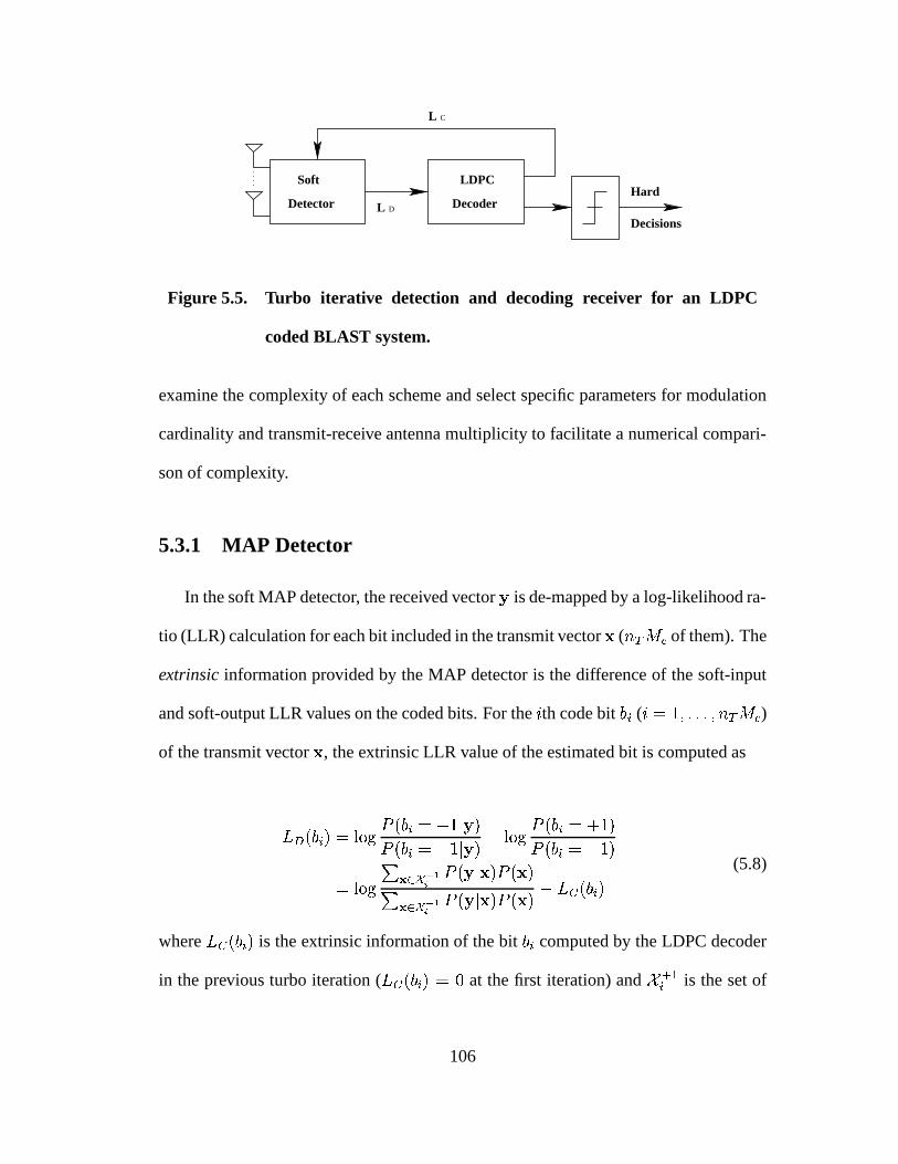
LDPCSoftHard
DecisionsL
L
Detector Decoder
C
D
Figure 5.5. Turbo iterative detection and decoding receiver for an LDPC
coded BLAST system.
examine the complexity of each scheme and select specific parameters for modulation
cardinality and transmit-receive antenna multiplicity to facilitate a numerical compari-
son of complexity.
5.3.1 MAP Detector
In the soft MAP detector, the received vector � is de-mapped by a log-likelihood ra-
tio (LLR) calculation for each bit included in the transmit vector � ( � � � of them). The
extrinsic information provided by the MAP detector is the difference of the soft-input
and soft-output LLR values on the coded bits. For the � th code bit� 9 ( � � ���(�(�(� � � � � )
of the transmit vector � , the extrinsic LLR value of the estimated bit is computed as
���� � 9 � � ) � ' � � � 9 � � �� � �
� � � 9 � �:�� � � � )�� ' � � � 9 � � � �� � � 9 � � � �
� ) � ' � ��� < �� � � � � � � � � � � � ��� " �� � � � � � � � � � � � � � � � 9 � (5.8)
where � � � � 9 � is the extrinsic information of the bit� 9 computed by the LDPC decoder
in the previous turbo iteration ( � � � � 9 � � � at the first iteration) and� � #9 is the set of
106

�� � � � / # vector hypotheses � having
� 9 � � � , (� / #9 is similarly defined). Based on the
extrinsic LLR of the code bits provided by the LDPC decoder and assuming the bits
within � are statistically independent of one another, the a priori probability � � � � can
be written as
� � � � � � � � I�� � # � � � � � � � � � I�� � # � � ��� � � � � ��� ��� � � � � � ��� / # (5.9)
where ��� ��� corresponds to the value (� ��� � � ) of the
�th bit in the vector � .
In the above LLR value calculation, the likelihood function � � � � � � is specified by
the multi-dimensional Gaussian pdf
� � � � � � � �� �� % � � � � � � � 5 � �� % �
� � � � � � � 7 � (5.10)
Note that for the LLR value calculation, only the term in the exponent is relevant; the
constant factor outside the exponent can be dropped.
Since the cardinality of the vector sets� � #9 and
� / #9 in (5.8) equals ��� � I / # , the
complexity of the soft MAP detector is exponential in the number of transmitter an-
tennas and the number of bits per constellation symbol. At each iteration, the MAP
detector has to compute the LLRs for � � � bits in each transmit symbol vector. With
an equal number of transmit and receive antennas, � � � � � � , evaluating (5.8)
involves the following steps:
for � � � to ��� I
1) Compute the a priori probability � � � � in (5.9): � � � � flops.
end
107

for � � � to � � �
2) Compute the LLR value in (5.8): � � ��� I flops.
end
In the above we do not consider the computation of the likelihood function � � � � � � .This is precomputed for all �
�� I hypotheses at the beginning of the iterative process
and has a cost of � � � � � � flops per vector hypothesis. We define a flop as a single
addition, subtraction, multiplication or division between two complex numbers. Table
lookups to� � � and
) � ' functions are not included in this complexity analysis. Then, the
(approximate) cost of the MAP detector per turbo iteration is� � � � � � � � � � I flops and
the initial cost of precomputing the likelihood functions for all hypotheses is� � � � �
� � ��� � � � I flops.
5.3.2 MMSE-SIC Detector
The suboptimal demodulator based on a minimum-mean square-error soft-interference
cancellation criterion is described in detail in [41] and [27]. Below we give a short re-
view and comment on its complexity.
The MMSE-SIC detector first forms soft estimates of the symbols transmitted from
the�th antenna (
� � ���(�(�)�)� � ) as
�� � � � 3���� � � ����� (5.11)
where�
is the complex constellation set and
� ����� � � I�
� � # ��� � � � � � � � � � � � � � � � � / #�� � I � � ��� � / # (5.12)
108

where�� � � indicates the value of the � th bit of symbol
�.
Then, for the�
th antenna, the soft interference from the other � ��� antennas is
canceled to obtain
� � � � �� ��� � # � ���� � �� � � � � � � � � � � ��� � # � ���� � ��� � � �� � � � � � � � (5.13)
A detection estimate � � of the transmitted symbol on the�
th antenna is obtained by
applying a linear MMSE filter � � to � � ,� � ��� �� � � �
�� ��
� � � � � � � ��� � # � ���� � � � �� � � � ��� � � �� � � � � �� � (5.14)
where � represents the conjugate transpose operator. The filter � � is chosen to minimize
the mean-square error between the transmit symbol� � and the filter output � � and is
given by
� � � 5 � ; � � � ��� � � � 7 / # � � (5.15)
where the covariance matrix � is
� � � diag 70� � � �� #�� � �(�(�)� �(� � � �� � / #�� � �(���(� � � �� � � #�� � �(�(�(� �(� � � �� � � � � 80� (5.16)
Observe that in (5.14), the first term represents the desired term, the second term is
residual interference from the other transmitter antennas and the last term is a phase ro-
tated noise term. As noted in [49], we can make the following Gaussian approximation
for the MMSE filter output � �� � �� ��� � �$� �� � (5.17)
where the variance � �� is given by
� �� � � ��� ��� � � (5.18)
109

Then, the extrinsic log-likelihood ratio computed by the MMSE-SIC detector for the
� th bit ( � �'���)�(�(� � � � ) of the symbol� � transmitted by the
�th antenna (
� � ���(�(�(� � � )
is
� �� � � � / #�� � I � � � � ) � ' � � � � � / #�� � I � � � � �� � � �
� � � � � / #�� � I � � � �:�� � � � � ) � ' � � � � � / #�� � I � � � � � �� � � � � / #�� � I � � � �:� �
� ) � ' 3�� � < �� � � � � � ��� � ����� 3���� " �� � � � � � ��� � ����� � � � � � � � / #�� � I � � � (5.19)
where� � #� is the set of � � I / # hypotheses
�for which the � th bit is
� � (� / #� is similarly
defined). In the above calculation of the extrinsic LLR value, the a priori probability
� ����� is given by (5.12) and the likelihood function � � � � � ��� is approximated by
� � � � � ��� � � � ��
� � � 5 � �� �� � � � � � � � 7 � (5.20)
Note that the MMSE-SIC detector has a lower complexity than the MAP detector.
This can be seen from (5.19) where the extrinsic LLR is computed from the scalar out-
put � � of the MMSE filter, in contrast with (5.8) where the extrinsic LLR is computed
from the received vector � . With an equal number of transmit and receive antennas,
� � � � � � , evaluating (5.19) involves the following steps:
for� � � to �
for � � � to � � I1) Compute the a priori probability � ����� in (5.12): � � � flops.
end
2) Evaluate the soft estimate in (5.11): � � � � I flops.
3) Cancel the soft estimates in (5.13): � � � flops.
4) Evaluate the matrix � �� � �" � � � � � � � � : � � 1 � � � � � � flops.
110

5) Solve � � � � � � for � � : � 1 ��� flops using Choleski factorization [17].
6) Compute the detection estimate � � : � � flops.
for � � � to� �
7) Compute the LLR value in (5.19): � � � � I flops.
end
end
Then, the (approximate) computational complexity of the MMSE-SIC detector is � � � �%� �
� � 1 � � � � � � � � � � ��� � � I � � � � ��� � � I flops per turbo iteration.
5.3.3 MMSE Suppression Detector
While the MMSE-SIC detector reduces the complexity of computing the extrinsic
LLR values from exponential to polynomial in the number of transmit antennas, it still
has the undesirable cost of re-evaluating the MMSE filter � � and updating � � with
each turbo iteration, as these depend on the soft estimates from the LDPC decoder
in the previous iteration. A simple linear MMSE suppression filter can significantly
reduce the complexity of the soft MIMO detector and incurs only a small performance
degradation as compared to MMSE-SIC.
In this case the MMSE suppression filter is evaluated only once, at the beginning
of the turbo iterative process, and applied to the received vector � to obtain a detection
estimate for the�
th antenna,
� � ��� �� � � (5.21)
111

No interference cancellation is performed and the linear MMSE filter � � is chosen to
suppress the co-antenna interference,
� � � 5 � ; � � � � � � 7 / # � � � (5.22)
As before, we make the Gaussian approximation of the soft MMSE filter output � � ,with the variance � �� as in equation (5.18), where � � is replaced by the new MMSE
filter. The extrinsic LLR values are computed exactly as in the case of the MMSE-SIC
detector using (5.19). Assuming � � � � � � , evaluating the LLR values involves the
following steps:
for� � � to �
for � � � to � � I1) Compute the a priori probability � ����� in (5.12): � � � flops.
end
for � � � to� �
2) Compute the LLR value in (5.19): � � � � I flops.
end
end
Then, the complexity per turbo iteration is� � � � � � � � � I flops. Moreover, the initial
cost of evaluating the MMSE suppression filters � � and the detection estimates � � is
� � � ��� � � � � flops. Note that the MMSE suppression detector reduces the complex-
ity per turbo iteration from ��� � � (for the MMSE-SIC detector) to �
���. Of course,
the overall complexity for the MMSE suppression scheme remains ��� � � because of
112
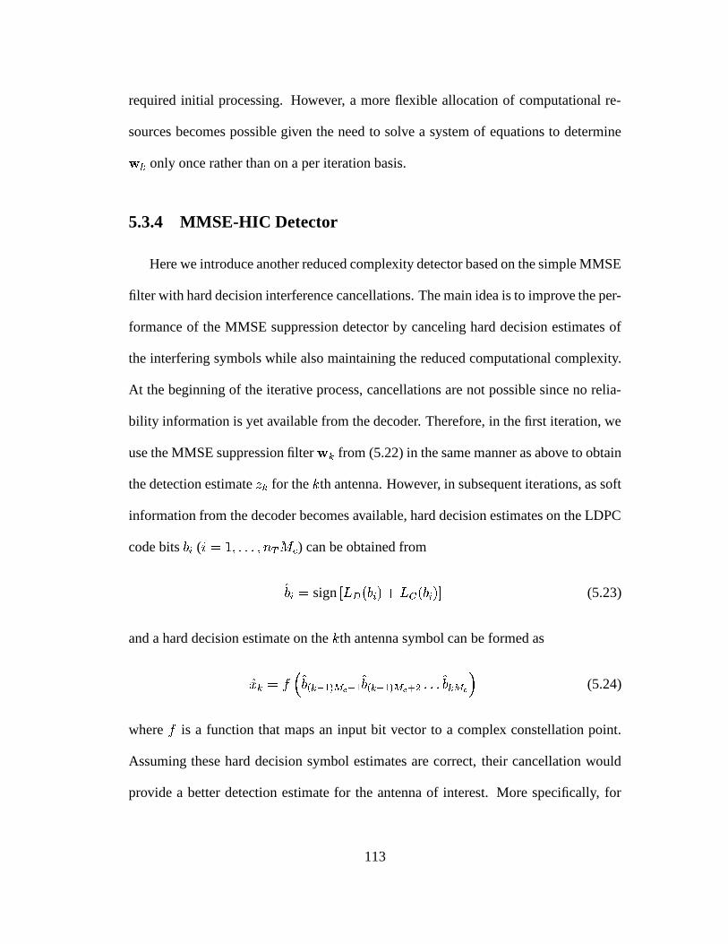
required initial processing. However, a more flexible allocation of computational re-
sources becomes possible given the need to solve a system of equations to determine
� � only once rather than on a per iteration basis.
5.3.4 MMSE-HIC Detector
Here we introduce another reduced complexity detector based on the simple MMSE
filter with hard decision interference cancellations. The main idea is to improve the per-
formance of the MMSE suppression detector by canceling hard decision estimates of
the interfering symbols while also maintaining the reduced computational complexity.
At the beginning of the iterative process, cancellations are not possible since no relia-
bility information is yet available from the decoder. Therefore, in the first iteration, we
use the MMSE suppression filter � � from (5.22) in the same manner as above to obtain
the detection estimate � � for the�th antenna. However, in subsequent iterations, as soft
information from the decoder becomes available, hard decision estimates on the LDPC
code bits� 9 ( � � ���)�(�(�)� � � � ) can be obtained from
�� 9 � sign � ��� � � 9 � � � � � � 9 � � (5.23)
and a hard decision estimate on the�th antenna symbol can be formed as
�� � � � ��� � � / #�� � I � # �� � � / #�� � I � � �(�)�
�� � � I (5.24)
where�
is a function that maps an input bit vector to a complex constellation point.
Assuming these hard decision symbol estimates are correct, their cancellation would
provide a better detection estimate for the antenna of interest. More specifically, for
113

the�th transmit antenna, the hard decision estimates of the other � � � interfering
antennas can be canceled to obtain
� � � � �� ��� � # � ���� � �� � � � (5.25)
and the new detection estimate � � can be obtained by maximum-ratio-combining,
� � �� �� � �� � � � � �
� �" � (5.26)
Observe that the assumption of correct hard decisions does not hold very well es-
pecially in the early stages of the iterative process. In order to avoid error propagation
due to incorrect hard decisions, it is very important that cancellations be performed
only when the reliability of the canceled symbols is high according to some cancella-
tion criterion. We experimented with different criteria for interference cancellation and
found that the following two methods give the best results:
� Average of LLRs
With this criterion, first the following average is computed and then compared to
a predetermined threshold value
� � � �� � �
� � � I�9 � # � � � � � 9 � � ��� � � (5.27)
The threshold� � is found experimentally as the threshold that yields the best
bit-error rate (BER) performance. Observe that a too low threshold value would
introduce undesirable error propagation due to incorrect cancellations, while a
too high threshold value would give the same performance as the MMSE sup-
pression detector since no cancellations are performed in this case.
114

� Probability of bit vector
With this criterion, the probability of a bit vector is first computed and then com-
pared to a threshold value
� � � � � � # � � �)�(� � � � � I � � � � � I�9 � # ��� � � � � � � � � � � � 9 � � � � / # ��� � � (5.28)
As before, the threshold� � is found experimentally to optimize the BER perfor-
mance.
The computational complexity of the MMSE-HIC detector is that of the MMSE
suppression detector plus the additional cost of checking the cancellation criterion every
turbo iteration and performing the hard decision interference cancellation whenever the
criterion is satisfied. Assuming � � � � � � , evaluating the LLR values involves the
following steps:
for� � � to �
1) Check the cancellation criterion in (5.27): � � � flops.
2) Cancel the hard decision estimates in (5.25): � � � flops.
3) Compute the detection estimate � � in (5.26):� � flops.
for � � � to � � I4) Compute the a priori probability � ����� in (5.12): � � � flops.
end
for � � � to� �
5) Compute the LLR value in (5.19): � � � � I flops.
end
115

end
Then, the worst-case computational complexity (assuming cancellations are performed
every iteration) is� � � 1 � � � � � � � � � � � � � � � � � � � � I flops per turbo iteration. The first
terms in this summation represent the additional complexity over the MMSE suppres-
sion detector. As in that case, there is an initial cost of � � � ��� � � � � flops to evaluate
the MMSE filters and the detection estimates.
In Table 5.2 we give a complexity comparison example based on a flop count for the
MAP, MMSE-SIC, MMSE suppression and MMSE-HIC detectors for � � � antenna
configurations with � � � � � � � , using QPSK modulation. For each detector, we provide
the initial cost (which is the cost of computations that must be done only once for all of
the iterations), the cost per turbo iteration, and the total computational cost assuming
��� iterations.
5.4 Performance Comparison of the Different Detectors
5.4.1 MI Performance of Different Detectors on parameterized 2 � 2
Channels
Points plotted as circles in Fig. 5.6 illustrate the 2 � 2 total excess MI (assuming
Gaussian alphabet signaling) for the � � �����(�)� optimized code of Table 5.1. Again,
per Fig. 5.3, operational mutual information varies more significantly with parameter �
as � approaches zero. This variation is manifested as a performance loss on � � � �
channels and is most severe for the MMSE-Supression detector. This is the simplest of
116

� � � � � � � � �
MAP initial � � � ��� �(� � �.��� �� ��� � �.� �
MAP per iteration ����� �� � � � �.��1 � � � � � �.� �
MAP total (30 iterations) � � ��� � �.��1 � ��� � � �.�%6 ��� ��� � �.� �
MMSE-SIC initial � � �
MMSE-SIC per iteration �(�� ��� ��� � �.� 1 ��� ��� � �.� �
MMSE-SIC total (30 iterations)� ����� � �(� 1 �� � � � �.� � ���� � � �.� 6
MMSE suppression initial� � � � � � � ��� � �(��1
MMSE suppression per iteration � � ����� ���%�
MMSE suppression total (30 iterations) ��� � � � �.��1 � � � � � �.�%1 ����� � � �.� �
MMSE-HIC initial� � � � � ������ � �.��1
MMSE-HIC per iteration �.� � ��� � ��� ��� � �.��1
MMSE-HIC total (30 iterations) � � ��� � �(��1 ��� ��� � �.� � � � � � � �.� �
Table 5.2. Cost (in flops) of computing the LLRs for different MIMO detectors.
117

the detectors as it does not employ feedback between the decoder and the detector. Note
that the MAP detector with feedback turned off (Fig. 5.4) exhibited a similar, though
less severe, performance loss on the � � � , � � � � channel.
0 0.2 0.4 0.6 0.8 10
0.25
0.5
0.75
1
1.25
1.5
1.75
2
Skew (λ2 / λ
1)
Tot
al E
xces
s M
I (B
its)
MAP MMSE−SICMMSE Sup
Figure 5.6. Simulation results showing excess MI vs. eigenvalue skew � at
BER � �(� /�� for different detectors (rate 1/3 length 15,000 ���
�����(�)� optimized code modulating QPSK on a 2 � 2 channel). The
MAP and MMSE-SIC detectors perform similarly with worst case
channels occurring when � � � under the � � � � rotation. The
MMSE only detector suffers the most severe degradation on the
� � � , � � � � since feedback is not employed to suppress the
co-channel interference present under this parameterization.
118

5.4.2 SNR and MI Performance of Different Detectors in Fast Rayleigh
Fading
In this section we examine the performance of LDPC coded BLAST systems using
the soft MIMO detectors introduced in the previous section. In our study, we assume
that the number of receive antennas is the same as the number of transmit antennas, i.e.
� � � � . The LDPC code used in the simulations is the rate- � ��� , length �.������� code
that was realized from the degree distribution given by the code labeled �3� �!���(�)� in
Table 5.1. The density evolution threshold for this code in AWGN is � � � � � dB. This
degree sequence was found via a linear program that sought the highest rate ensemble
under a given threshold and maximum left and right node degree constraints [11]. In
order to acquire a given rate goal, the density evolution initial mean was adjusted to
achieve the desired rate. The mapping in all our simulations is a Gray-labeled QPSK
constellation. The resulting spectral efficiency is� ��� bits/channel use.
We assume a fast Rayleigh fading scenario, where the channel matrix is realized
independently from one transmission time to the next. We compare our bit-error rate
results with the theoretical channel capacity limit. Under the fast fading assumption,
the theoretical capacity limit is the ergodic channel capacity given by [42],
� � ' )�� ' � det5 � � � ;
� � � � 7 * (5.29)
where the expectation is over the entries of � .
Figs. 5.7, 5.8, 5.9, and 5.10 show the BER performance versus average SNR per
receiver antenna on � � � , � � � , � ��, and � � � fast fading Rayleigh channels. On these
plots we also show the channel capacity at the corresponding transmission bit rate for
119

−2 −1.5 −1 −0.5 0 0.5 1 1.5 210
−4
10−3
10−2
10−1
100
SNR (dB)
BE
R
MMSEMMSE−HICMMSE−SICMAPCapacity
Figure 5.7. Performance of LDPC coded BLAST for � � � MIMO system with
MAP, MMSE-SIC, MMSE-HIC and MMSE suppression detec-
tors.
these systems. As expected, the MAP detector yields the best performance, which is �
dB away from the theoretical capacity at BER � �(��/�� on the � � � channel. We note that
the MMSE-SIC detector has essentially the same performance as the MAP detector on
the � � � , � � � , and�
��
systems. For the � � � channel the computational complexity
associated with the MAP detector is prohibitive and this result was not simulated.
Our results differ from the results reported in [27] where a system based on the
MMSE-SIC detector has a performance degradation (less than � dB) compared to a
system based on the MAP detector. We attribute this difference to the fact that in [27]
a detector iteration is performed only after a number of decoder iterations, whereas in
our work every decoder iteration is followed by a detector iteration.
120

−2 −1.5 −1 −0.5 0 0.5 1 1.5 210
−4
10−3
10−2
10−1
100
SNR (dB)
BE
R
MMSEMMSE−HICMMSE−SICMAPCapacity
Figure 5.8. Performance of LDPC coded BLAST for � � � MIMO system with
MAP, MMSE-SIC, MMSE-HIC and MMSE suppression detec-
tors.
Moreover, our simulation results show that the very low complexity MMSE sup-
pression detector has a performance loss of only ���� dB or less. This loss is approxi-
mately cut in half if the MMSE-HIC detector with an optimized cancellation threshold
is used instead. In fact, in the � � � system, the MMSE-HIC detector performance is
very close to the MAP and MMSE-SIC detectors.
Though the majority of this section has focused on a comparison of the performance
of the different detectors in terms of SNR in Rayleigh fast fading we again emphasize
the robustness of the codes as measured in terms of excess mutual information via
Fig. 5.11.
The cases plotted in this figure are contrasted from the exhaustively parameterized
121

−2 −1.5 −1 −0.5 0 0.5 1 1.5 210
−4
10−3
10−2
10−1
100
SNR (dB)
BE
R
MMSEMMSE−HICMMSE−SICMAPCapacity
Figure 5.9. Performance of LDPC coded BLAST for�
��
MIMO system with
MAP, MMSE-SIC, MMSE-HIC and MMSE suppression detec-
tors.
2 � 2 case where we were able to determine best and worst case channels. Here, instead,
all channel results are average together in conjunction with the Rayleigh distribution.
Note that under MAP and MMSE-SIC detection, the excess MI per antenna remains
essentially constant, at 0.25 bits, as the number of transmit/receive antennas increases
from 2 to 4. MAP detector results were not computed (due to prohibitive complexity)
for the 8 � 8 case.
122

−2 −1.5 −1 −0.5 0 0.5 1 1.5 210
−4
10−3
10−2
10−1
100
SNR (dB)
BE
R
MMSEMMSE−HICMMSE−SICCapacity
Figure 5.10. Performance of LDPC coded BLAST for � � � MIMO system with
MMSE-SIC, MMSE-HIC and MMSE suppression detectors.
5.5 Conclusion
In this chapter we have shown that the excess mutual information required to achieve
a bit error rate of �(� /�� on the 2 � 2 channel with a particular LDPC code varies by ap-
proximately 0.5 bits (with a total rate 4/3 code) between the best and worst case channel
when excess MI is measured against Net constrained capacity. However, excess MI is
essentially constant when measured against PID constrained capacity. Code perfor-
mance very closely tracks available operating mutual information. Therefore, LDPC
codes themselves are robust to channel variation. The information loss incurred during
joint PDF marginalization to individual bit PDFs in the detection process is the root
cause of excess mutual information variation with eigenskew.
123

2x2 3x3 4x4 8x80.2
0.25
0.3
0.35
0.4
Exc
ess
MI p
er A
nten
na
Antenna Configuration
MAPMMSE−SICMMSE−HICMMSE−Sup
Figure 5.11. Performance of different detectors across increasing antenna
multiplicities in terms of excess mutual information per transmit
antenna in Rayleigh fading. Each excess MI is measured from
constrained ergodic Rayleigh capacity for the given channel.
We have also shown that several variants of LDPC coded BLAST systems with iter-
ative detection and decoding perform roughly � dB from the theoretical capacity of the
Rayleigh MIMO channel. The soft MAP detector is optimal, however the MMSE-SIC
detector exhibits similar performance and has a lower overall computational complex-
ity. The MMSE suppression and MMSE-HIC detectors offer yet lower complexities,
for relatively small performance penalties. As an example, for the�
��
system, con-
sidering the MAP detector as the norm, the total complexity (with ��� iterations) of
the MMSE-SIC detector is � times lower, that of the MMSE-HIC detector is �%� times
124

lower, and that of the MMSE suppression detector is � � times lower. A performance
loss of around ���� dB is observed for the MMSE suppression detector. This loss is cut
approximately in half by an MMSE-HIC detector using a carefully chosen cancellation
threshold.
Appendix - Operational Mutual Information in Systems
Without Prior Information Feedback
Theorem 3 The mutual information available to an iterative decoder for the case of
a generalized Gaussian channel without feedback between the detector and decoder is
given by
�� ��� ��� � � � � ��� � I / #� � � � � ��� � � � � ��� � � � � (5.30)
where� � � � � calls out the
�th bit in the transmit vector
�which carries a total of � � � �
bits, and�
,�
are RVs and � is the given channel matrix.
Proof: Consider the decoding scenario where the instantaneous mutual infor-
mation entering the decoder due to each received vector � � is given by�� � (here we
re-introduce time index�
),
�� � �� � � I / #� � � � �� � where
�� � � � �� � � � � � ����� � � � �
� � � � � � � � � � � � � ��� � (5.31)
125

Observe that�� � is the sum of the instantaneous marginalized bit reliability mutual in-
formations. The marginalization step reduces the information entering the decoder
at each receive time�
from the instantaneous vector-wise joint mutual information,
� � � � � � � � � � � , to the sum of the instantaneous bitwise mutual informations, or�� � . Ex-
plicitly,�� � is defined as (for uniform �
� � � � � � ��� ,�� � �
��� � I / #� � � � ����������
� � � � # � �� � � � � � � � � � � � � �
)�� ' � � �� � � � � � � � � � � � � ���
� )�� ' � � � � � ����������� (5.32)
To complete the proof, observe that the expectation of the instantaneous mutual infor-
mation converges to the ergodic mutual information of the sum of the individual bit
planes in the limit of infinite sample size � ,
��
�/ #�� � � �� � � � � ����
�
��� � I / #� � � � � ��� � � � � ��� � � � � (5.33)
An exchange in the order of the two outermost summations in (5.33) left-hand-side and
(5.32) respectively yields this asymptotic result. Hence the average given by (5.30) is
the information available to the closed iterative decoder.
126

Bibliography
[1] A. A. AlRustamani, A. Stefanov, and B. R. Vojcic. Turbo-greedy coding for
multiple antenna systems. In Proceedings of ICC, volume 6, pages 1684 –1689,
June 2001.
[2] D. M. Arnold, E. Eleftheriou, and X. Y. Hu. Progressive edge-growth Tanner
graphs. in Proc. IEEE Global Telecommun. Conf., San Antonio, TX, Nov. 2001,
2:995–1001.
[3] S. Benedetto, D. Divsalar, G. Montorsi, and F. Pollara. Serial concatenation of
interleaved codes: performance analysis, design, and iterative decoding. IEEE
Trans. Inform. Theory, 44:909–926, May 1998.
[4] C. Berrou, A. Glavieux, and P. Thitimajshima. Near Shannon limit error-
correcting coding and decoding: Turbo codes. in Proc. IEEE Int. Conf. Commun.,
Geneva, Switzerland, pages 1064–1070, May 1993.
[5] Jones C., Matache A., Tian T., Villasenor J., and Wesel R. D. The universality of
ldpc codes on wireless channels. In Proceedings of MilCom, Oct 2003.
127

[6] Jones C., Tian T., Matache A., Wesel R. D., and Villasenor J. Robustness of ldpc
codes on periodic fading channels. In Proceedings of GlobeCom, Nov 2002.
[7] J. Chen, A. Dholakia, E.Eleftheriou, M. Fossorier, and X.-Y. Hu. Near optimum
reduced-complexity decoding algorithms for LDPC codes. in Proc. IEEE Int.
Sym. Inform. Theory, Lausanne, Switzerland, Jul. 2002.
[8] J. Chen and M. Fossorier. Density evolution for BP-based decoding algorithms
of LDPC codes and their quantized versions. in Proc. IEEE Globecom, Taipei,
Taiwan, Nov. 2002.
[9] J. Chen and M. Fossorier. Near optimum universal belief propagation based de-
coding of LDPC codes. IEEE Trans. on Comm., 50(3), Mar. 2002.
[10] A. Chini. Multi Carrier Modulation in Frequency Selective Channels. PhD thesis,
Carleton Institute for Electrical Engineering, Ottawa, Sept. 1994.
[11] S.Y. Chung, T. Richardson, and R. Urbanke. Analysis of sum-product decoding
of low-density parity-check codes using a gaussian approximation. IEEE Trans.
on Inform. Theory, 47:657–670, Feb 2001.
[12] C. Di, D. Proietti, E. Telatar, T. Richardson, and R. Urbanke. Finite length analysis
of low-density parity-check codes on the binary erasure channel. IEEE Trans.
Inform. Theory, 48:1570–1579, June 2002.
[13] L. Dong-U, J. Villasenor, and W. Luk. A hardware Gaussian noise generator for
128

exploring channel code behavior at very low bit error rates. In In proceedings of
FCCM, May 2003.
[14] E.Eleftheriou, T. Mittelholzer, and A. Dholakia. A reduced-complexity decoding
algorithm for low-density parity-check codes. IEE Electron. Letters, 37:102–104,
Jan. 2001.
[15] G. J. Foschini and M. J. Gans. On limits of wireless communications in a fading
environment when using multiple antennas. Wireless Personal Communications,
6:311–335, 1998.
[16] C. Fragouli and R. D. Wesel. Bit vs. symbol interleaving for parallel concatenated
trellis coded modulation. in Proc. IEEE Global Telecommun. Conf., San Antonio,
TX, Nov. 2001, 2:931–935.
[17] G. H. Golub and C. F. van Loan. Matrix Computations. Baltimore, MD: Johns
Hopkins Univ. Press, third edition, 1996.
[18] R.G. Gallager. Low-density parity-check codes. IRE Trans. Inform. Theory, IT-
8:21–28, Jan 1962.
[19] C. Jones, R. Tian, R. Wesel, and J. Villasenor. The Universal Operation of LDPC
Codes in Scalar Fading Channels. In Submission to the IEEE Transactions on
Communications, Oct 2003.
[20] J.H. Kang and W.E. Stark. Turbo codes for coherent fh-ss with partial band inter-
ference. In Proceedings of Military Communications Conference, Nov 1997.
129

[21] ”Kose, C., and R.” Wesel. Universal space-time trellis codes. In Proceedings of
GlobeCom, Nov 2002.
[22] ”Kose, C., and R.” Wesel. Universal space-time trellis codes. IEEE Transactions
on Information Theory, Special Issue on Space-Time Transmission, Reception,
Coding and Signal Design, Nov. 2003.
[23] C. Kose, W.Y. Weng, and R.D. Wesel. Serially concatenated trellis coded modu-
lation for the compound periodic erasures channel. In Proceedings of ICC, May
2003.
[24] Y. Kou, S. Lin, and M. Fossorier. Low-density parity-check codes based on finite
geometries: a rediscovery and new results. IEEE Trans. Inform. Theory, 47:2711–
2736, Nov. 2001.
[25] F.R. Kschischang, B.J. Frey, and H.A. Loeliger. Factor graphs and the sum-
prodcut algorithm. IEEE Trans. on Inform. Theory, 47:498–519, Feb 2001.
[26] L. Lampe, R. Schober, and R. Fischer. Multilevel coding for multiple-antenna
transmission. In Proceedings of 2002 International Symposium on Information
Theory, volume 1, July 2002.
[27] B. Lu, G. Yue, and X. Wang. Performance analysis and design optimization of
LDPC coded MIMO OFDM systems. to appear in EURASIP JASP, 51(11).
[28] M.G. Luby, M. Mitzenmacher, M.A. Shokrollahi, and D.A. Spielman. Improved
130

low-density parity-check codes using irregular graphs. IEEE Trans. on Inform.
Theory, 47:569–584, Feb 2001.
[29] D.J.C. Mackay. Good error correcting codes bases on very sparse matrices. IEEE
Trans. on Inform. Theory, 45:399–431, Mar 1999.
[30] D.J.C. MacKay, S.T. Wilson, and Davey M.C. Comparison of constructions of
irregular Gallager codes. IEEE Trans. on Comm., 47(10):498–519, October 1999.
[31] Y. Mao and A. H. Banihashemi. A heuristic search for good low-density parity-
check codes at short block lengths. in Proc. IEEE Int. Conf. Commun., Helsinki,
Finland, June 2001.
[32] G. A. Margulis. Explicit construction of graphs without short cycles and low
density codes. Combinatorica, 2(1):71–78, 1982.
[33] A. Matache and R. D. Wesel. Universal Trellis Codes for Diagonally Layered
Space-Time Systems. IEEE Transactions on Signal Processing, Special Issue on
MIMO Wireless, Nov. 2003.
[34] J. Pearl. Probabilistic Reasoning in Intelligent Systems: Networks of Plausible
Inference. Morgan Kaufmann, San Francisco, CA, 1998.
[35] M. Pursely and J. Skinner. Decoding strategies for turbo product codes in
frequency-hop wireless communications. In Proceedings of ICC, May 2003.
[36] T. Richardson, A. Shokrollahi, and R. Urbanke. Design of capacity approaching
131

irregular low density parity check codes. IEEE Trans. on Inform. Theory, 47:618–
637, Feb 2001.
[37] T. Richardson and R. Urbanke. Efficient encoding of low-density parity-check
codes. IEEE Trans. on Inform. Theory, 47:638–656, Feb 2001.
[38] T. Richardson and R. Urbanke. The capacity of low-density parity-check codes
under message passing decoding. IEEE Trans. on Inform. Theory, 47:599–618,
Feb 2001.
[39] W.L. Root and P.P Varaiya. Capacity of classes of Gaussian channels. SIAM J.
Appl. Math, 16(6):1350–1393, November 1968.
[40] M. Sellathurai and S. Haykin. TURBO-BLAST for high speed wireless commu-
nications. In Proceedings of WCNC, volume 1, pages 315–320, Sept 2000.
[41] M. Sellathurai and S. Haykin. Turbo-BLAST for wireless communications: the-
ory and experiments. IEEE Trans. Signal Proc., 50(10):2538–2546, Oct 2002.
[42] I. E. Telatar. Capacity of multi-antenna Gaussian channels. European Trans.
Telecommun., 10(6):585–595, Nov.-Dec. 1999. Available: http://mars.
bell-labs.com/cm/ms/what/mars/papers/proof/.
[43] S. Ten Brink and B. Hochwald. Achieving near-capacity on a multiple-antenna
channel. IEEE Trans. on Comm., 51(3):389–399, Mar. 2003.
[44] Tian T., Jones C., Villasenor J., Wesel R. D. Characterization and selective avoid-
132

ance of cycles in irregular LDPC code construction. Submitted to IEEE Trans. on
Comm., 2002.
[45] Tian T., Jones C., Villasenor J., Wesel R. D. Characterization and selective avoid-
ance of cycles in irregular ldpc codes. In Proceedings of ICC, May 2003.
[46] A. van Zelst, R. van Nee, and G. A. Awater. Turbo-BLAST and its performance.
In Proceedings of VTC, volume 2, pages 1282–1286, May 2001.
[47] A. Vardy. The intractability of computing the minimum distance of a code. IEEE
Trans. Inform. Theory, 43:1757–1766, Nov. 1997.
[48] U. Wachsmann, R. Fischer, and J. Huber. Multi-Level Codes: Theoretical Con-
cepts and Practical Design Rules. IEEE Trans. on Inform. Theory, 45:1361–1391,
May 1999.
[49] X. Wang and H. V. Poor. Iterative (Turbo) soft interference cancellation and de-
coding for coded CDMA . IEEE Trans. on Comm., 47:1046–1061, July 1999.
[50] W.Y. Weng, C. Kose, and R.D. Wesel. Serially concatenated trellis coded modu-
lation for the compound periodic erasures channel - in submission. IEEE Trans.
on Comm.
[51] R. Wesel. Trellis Code Design for Correlated Fading and Achievable Rates for
Tomlinson-Harashima Precoding. PhD thesis, Stanford University, Department
of Electrical Engineering, Palo Alto, Aug. 1996.
133
[52] Wesel, R.D. and Cioffi, J.M. Trellis codes design for periodic interleavers. IEEE
Comm. Letters, 3:103–105, April 1999.
[53] Wesel, R.D. and Liu, X. and Shi, W. Trellis codes for periodic erasures. IEEE
Trans. on Comm., 48:938–947, June 2000.
[54] M. Yang and W. E. Ryan. Lowering the error-rate floors of moderate-length high-
rate irregular LDPC codes. In In proceedings of IEEE Int. Symp. Infor. Theory,
Yokohama, Japan, June 2003.
134