111CHAPITRE D'ÉQUATION 1 SECTION 1SEISMIC RESPONSE ASPECTS FOR DESIGN AND ASSESSMENT ASSESSMENT

Introduction (Jim)

Soil modellingAs explained in chapter 3 of the document soil characterization is a complex task and, depending on the choice of the soil constitutive model used for the analyses, the number of parameters to determine may vary to a large extent and degree of complexity (see table 3.3). Therefore, it is important that the level of efforts put in the determination of the soil characteristics be adapted to the needs without overshadowing the essential features of soil behaviour. In any case, it is essential that soil characteristics be determined by site specific investigations including field tests and laboratory tests, which should, as far as possible, yield coherent soil characteristics; any incoherence should be analysed and explained. Laboratory tests and field tests shall not be opposed to each other but used in combination since each of them has its own merit, limitation and range of applicability (see Figure 3.10). Special attention must be paid to the characterization of manmade backfills for which the characteristics can only be measured and determined provided enough specifications are available in terms of material source, identification, and compaction.

In several regions of the world the design earthquake may represent a moderate level earthquake which will induce only small to moderate strains in the soil profile. In others, highly seismic, regions the design earthquake may represent a strong motion event. These features should be considered when defining the soils parameters and associated investigations needed for design. In the first instance (moderate event), and as indicated in section 3.3, the most appropriate constitutive model will be the equivalent viscoelastic linear model (EQL). This model, which represents the state of practice, is simple enough to be amenable to the large number of parametric and sensitivity analyses required to account for the variability of soil properties (see section 8.6.2). It must be remembered that the uncertainty on the elastic properties is not the single parameter that needs to be considered: large uncertainties exist in the determination of the nonlinear shear stress–shear strain curves (or equivalently G/Gmax and damping ratio curves used to define the equivalent linear model). It is strongly recommended to measure these curves on undisturbed samples retrieved from the site and not to rely exclusively on published results; however, comparisons with published results are useful to define the possible variation of the curves and to assess the possible impact of such variations on the site response. It would be very uncertain to attempt to relate the domain of validity of the EQL model to some earthquake parameter (like PGA) since the strains also strongly depend on the material: some materials are “more linear” than others (e.g. highly plastic clay). However, for a preliminary estimate, PGA’s less than 0.2 –0.30g may be considered as moderate earthquakes for which the EQL model is relevant. However, in general, validity of the equivalent linear model has to be checked at the end of the analyses by comparing the induced shear strain to a threshold strain beyond which the constitutive model is no longer valid. Chapter 3 has proposed to fix that threshold strain to twice the reference shear strain (see chapter 3 for definition of the reference shear strain) and one example in the appendix on site response illustrates this aspect (see also section 8.3.2); note also that, if in a 1D model the definition of the shear strain is

straightforward, in a 3D situation it is proposed to define the “shear strain”, to be compared to the threshold strain, as the second invariant of the deviatoric strain tensor.

In highly seismic areas, it is most likely that the induced motions will be large enough to induce moderate to large strains in the soil profile. Therefore, the EQL model may not be appropriate to represent the soil behaviour. True nonlinear soil models are required to analyse soil structure interaction response. As indicated in chapter 3, numerous nonlinear models exist and the choice cannot be unique; it is strongly recommended that at least two different constitutive models be used by possibly two different analysts. The models should be validated for different stress paths, not only with respect to shear strain–shear stress behaviour but also with respect to volumetric behaviour, and their limitations should be fully understood by the analysts. Furthermore, it is highly desirable, although not mandatory, that the models possess a limited number of parameters easily amenable to determination and be based on physical backgrounds. As it is well known that soil response is highly sensitive to the chosen model, it is essential that uncertainty in the parameters, especially those with no physical meaning, be assessed through parametric studies. An example of a nonlinear constitutive model is described in the appendix along with the examples on site response analyses.

Free field ground motions

Approaches 1, 2, 3 (Jim)

1D modelA 1D soil column is used to develop examples, presented in appendix 1, illustrating the differences between the various approaches to 1D site response analyses. The soil profile consists of 30.0m of sandy gravel overlying a 20m thick layer of stiff, overconsolidated, clay on top of a rock layer considered as a homogeneous halfspace (Figure 8-1). The water table is located at a depth of 10.0m below the ground surface. The incident motion is imposed at an outcrop of the halfspace in the form of an acceleration time history. The soil constitutive models include an equivalent linear model, a nonlinear model for 1–phase medium and a nonlinear model for 2–phase (saturated) medium.

Under the assumption of vertically propagating shear waves, the numerical model is a one-dimensional geometric model; however, to reflect the coupling between the shear strain and volumetric strains each node of the model possesses two (1-phase medium or 2-phase undrained layer) or four (2-phase medium pervious layer) degrees of freedom corresponding to the vertical and horizontal displacements (respectively vertical and horizontal translations of solid skeleton and vertical and horizontal velocities of the fluid).

The purposes of the analyses are to:

Compare equivalent linear and nonlinear constitutive models;Show the differences between total vs effective stress analyses; Show for a 2–phase medium the impact of the soil permeability;Compare the predicted vertical motion assuming P-wave propagation to the motion calculated from the horizontal motion with V/H GMPEs (Gülerce & Abrahamson).

Figure 8-1: Soil profile for illustrative examples on 1D site response analyses

Results are compared in terms of 5% damped ground surface response spectra, pore pressure evolution in time at mid depth, horizontal and vertical displacements at the ground surface.

The following Table 8–1 summarizes the different analysed cases. All the nonlinear analyses are run with the software Dynaflow; the equivalent linear analyses are run with SHAKE.

Case 1a – 1b 2a – 2b 3 4 5 6

Continuum 1-Phase1-Phase 2-Phase

2-Phase 2-Phase 2-Phase 2-Phase

Model Total stresses

Effective stresses

Effective stresses

Effective stresses

Effective stresses

Effective stresses

Constitutive relationship

Equivalent linear/

nonlinearElastoplastic Elastoplastic Elastoplastic Elastoplastic Elastoplastic

Permeability (m/s) - 0 10-5 10-4 10-3 10-2

Input motion Horizontal Horizontal Horizontal Horizontal Horizontal Horizontal

Software ShakeDynaflow

Dynaflow Dynaflow Dynaflow Dynaflow Dynaflow

Case 6a – 6b 7a – 7b 8 9

Continuum 1-Phase1-Phase2-Phase

2-Phase 2-Phase

Model Total stresses

Effective stresses

Effective stresses

Effective stresses

Constitutive Equivalent Elastoplastic Elastoplastic Elastoplastic

relationship linear/ linear

Permeability (m/s) - 0 10-5 10-2

Input motion Horizontal + vertical

Horizontal + vertical

Horizontal + vertical

Horizontal + vertical

Software ShakeDynaflow

Dynaflow Dynaflow Dynaflow

Table 8-1:Summary of analysed cases

Comparison EQL / NL (cases 1a–1b)The example is used to point out that, beyond some level of shaking, EQL solutions are not valid. Figure 8-2 illustrates the comparison in terms of ground surface response spectra calculated for 3 increasing amplitudes of the input motion. This figure and additional figures presented in the appendix show that, as long as the input motion is not too strong (here pga ~ 0.20g), the EQL and NL solutions do not differ significantly. For 0.25g differences start to appear in the acceleration response spectra: high frequencies are filtered out in the EQL solution and a peak appears at 3Hz corresponding to the natural frequency of the soil column. At 0.5g the phenomena are amplified with a sharp peak at 2.8Hz in the EQL solution. Filtering of the high frequencies by the EQL analysis has been explained in chapter 3.4: they are dumped because the damping ratio and shear modulus are based on the strain, which is controlled by low frequencies, and the same damping is assigned to all frequencies. High frequency motions induce smaller strains and therefore should be assigned less damping.

Figure 8-2: Comparison of ground surface response spectra between EQL and NL analyses

The value of the pga threshold should not be considered as a universal value: it depends on the material behaviour; as explained in the main document (section 3.3.1), the fundamental parameter to look at is the induced shear strain, or better the reference shear strain r. The maximum shear strain calculated as a function of depth for each run is plotted in Figure 8-3 below. When the amplitude of the input motion is smaller than 0.20g, the maximum induced shear strain remains smaller than 10–3, which was indicated as the upper bound value for which equivalent linear analyses remain valid and, indeed, equivalent linear and nonlinear analyses give similar results. When the amplitude of the input motion is equal to 0.50g, the maximum induced shear strain raises up to 3.4 10–3 at 20m depth; at that depth the reference shear strain is equal to 10–3 (calculated from table 3 in the appendix) and therefore the induced shear strain is larger than two times the reference shear strain. For an input motion of 0.25g, the maximum shear strain at 20m depth is approximately equal to 2r and equivalent linear analyses and nonlinear analyses start to diverge.

Figure 8-3: Maximum shear strain versus depth for 3 input accelerations levels

Total vs effective stress analyses (cases 1a–2a)The analyses presented in the appendix show that at low level of excitation (pga ≤0.25g) both solutions (total or effective stress analyses) are comparable except of course for the pore pressure build up which cannot be predicted by the total stress analysis. At pga =0.50g differences appear in the acceleration response spectra and in the vertical displacements (Figure8-4, left).

It can be concluded that effective stress analyses are not needed for low level of excitation but are important for high levels, when the excess pore pressure becomes significant.

For an impervious material the effective stress analyses carried out assuming either a 1–phase medium or a 2–phase medium (case 2a–2b) do not show any significant difference (Figure 8-4, right). Based on the results of other analyses, not presented herein, this statement holds as long as the permeability is smaller than approximately 10–4 m/s. Therefore 2–phase analyses are not required for those permeabilities.

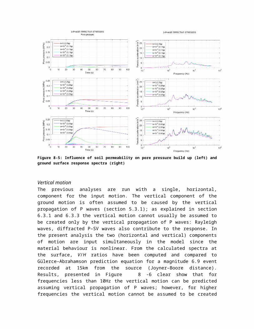
The impact of the value of the permeability appears to be minor on all parameters except the excess pore pressure (Figure 8-5). It is only for high permeabilities (10–2m/s) and high input excitations that differences appear in the acceleration response spectrum and, to a minor extent, in the vertical displacement.

Figure 8-4: Comparison of ground surface response spectra for effective and total stress analyses (left) and 1–Phase versus 2–Phase medium (right)

Figure 8-5: Influence of soil permeability on pore pressure build up (left) and ground surface response spectra (right)

Vertical motionThe previous analyses are run with a single, horizontal, component for the input motion. The vertical component of the ground motion is often assumed to be caused by the vertical propagation of P waves (section 5.3.1); as explained in section 6.3.1 and 6.3.3 the vertical motion cannot usually be assumed to be created only by the vertical propagation of P waves: Rayleigh waves, diffracted P–SV waves also contribute to the response. In the present analysis the two (horizontal and vertical) components of motion are input simultaneously in the model since the material behaviour is nonlinear. From the calculated spectra at the surface, V/H ratios have been computed and compared to Gülerce–Abrahamson prediction equation for a magnitude 6.9 event recorded at 15km from the source (Joyner–Boore distance). Results, presented in Figure 8-6 clear show that for frequencies less than 10Hz the vertical motion can be predicted assuming vertical propagation of P waves; however, for higher frequencies the vertical motion cannot be assumed to be created only by the vertical propagation of P waves: Rayleigh waves, diffracted P–SV waves also contribute to the response.

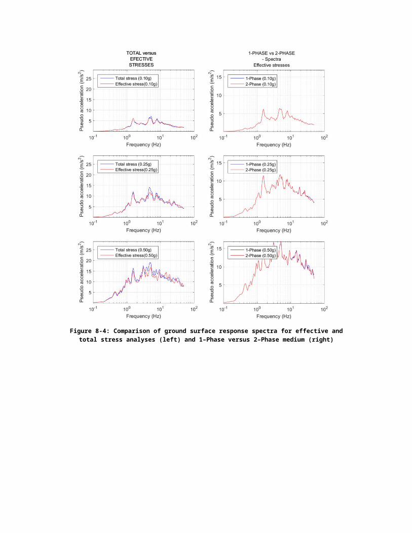
Figure 8-6: Computed V/H ratios compared to statistical V/H ratios (red line)

Lightly damped profiles The purpose of this example is to show that for nearly elastic materials, the choice and modelling (hysteretic, Rayleigh) of damping is critical for the site response. The “soil” column is composed of one layer of elastic rock material (2km thick with VS=2000m/s) overlying a halfspace with VS =3000m/s. It is subjected to a real hard rock record recorded in Canada and provided by Gail Atkinson: record OT012-HNG with a duration of 60s and a maximum acceleration equal to 0.03g; although pga is very small it has not been scaled up since all calculations presented in this example are linear. The record, its 5% damped response spectrum, and its Fourier amplitude spectrum are shown in the appendix.

Several methods are used for the calculations and illustrated on the rock column:

Pure elastic calculation with a time domain solution obtained with Dynaflow and two meshes: one with ten elements per wave length (element size 5m) and one with 20 elements per wave length (element size 2.5m); differences between both meshes are shown to be negligible and only the results with 10 elements per wave length are presented;Pure elastic calculation in the frequency domain with the Exponential Window Method (EWM) developed by Eduardo Kausel and introduced in the TECDOC (section 3.4);Viscoelastic calculation with 0.1% damping in the rock layer (the halfspace is still undamped) with a frequency domain solution: classical FFT (SHAKE) and EWM;Viscoelastic calculation with 1% damping in the rock layer (the halfspace is still undamped) with a frequency domain solution: classical FFT (SHAKE) and EWM;Numerical damping in the time domain analysis with Dynaflow (Newmark’s parameter setequal to 0.55 instead of 0.50 for no numerical damping);

Rayleigh damping (stiffness proportional) in the time domain analysis calibrated to yield 1% damping at two times the fundamental frequency of the layer, i.e. 0.5Hz.

Results are presented in terms of 5% damped ground surface response spectra (Figure 8-7).

Figure 8-7: Influence of damping modelling and numerical integration method on ground surface response spectra

Surface motions are very sensitive to low damping values, in the range 0% to 0.1%. For pure elastic calculation either the time domain solution (without numerical damping) or the EWM should be used; the agreement is good up to 25Hz; above that value they slightly differ but this may be due to filtering by the mesh in the time domain solution. For very lightly damped systems (0.1%), there is only one reliable method, the EWM; damping cannot be controlled in the time domain solution and the classical FFT overdamps the frequencies above 8Hz (in that case). For lightly damped systems (1%), the classical FFT and the EWM perform equally well. However, the EWM is much faster and does not require trailing zeroes to be added to the input motion; the duration of this quiet zone might be a cause of errors in FFT calculations if not properly chosen. Finally, Rayleigh damping should never be used for damped systems in time domain analyses; it might even be better to rely on numerical damping, but the exact damping value implied by the choice of the Newmark integration parameter is not known because it is frequency dependent (proportional to frequency for the present analysis).

Last but not least, from a practical standpoint, soils or rock with very low damping represent a very critical situation because the exact amount of damping in very stiff rock (0%, 0.1%, 1% ?) will never be known (or measured) with sufficient accuracy and the results are very sensitive to this choice above 1Hz.

2D models This example is presented to outline the importance of topographic effect. Motions are calculated at the location in the middle of a valley (see figure in the appendix) where a marked topography exists. Calculations are made assuming

a/ a 1D model, extracted from the soil column at the examined location, and an equivalent linear constitutive model,

b/ a 2D model, including the whole valley shown in the figure, with the strain compatible soil properties retrieved from the 1D–EQL analyses,

c/ the same 2D model as above but with a fully nonlinear constitutive model for the soil.

Ground surface response spectra calculated for these three assumptions are depicted in Figure8-8.

Figure 8-8: Influence of surface topography on ground surface response spectra

The calculated surface spectra clearly indicate that the 1D model is unable to predict the correct answer except for long periods, above 1.5s; at these periods, scattering of the incoming wave by the topography is insignificant. They also indicate that the main difference between the spectra arise from the geometric model rather than from the constitutive model, although the 2D linear model should be regarded with caution because damping is modelled as Rayleigh damping while in the 2 other analyses frequency independent damping is considered.

3 times 1D (Boris)Three Dimensional Seismic Motions and Their Use for 3D and 1D SSI ModelingPresent below is a simple study that emphasizes differences between 3D and 1D wave fields, and points out how this assumption (3D to 1D) affects response of a generic model NPP. It is noted that a more detailed analysis of 3D vs. 3×1D vs. 1D seismic wave effects on SSI response of an NPP is provided by (Abell et al., 2016).

Assume that a small scale regional models is developed in two dimensions (2D). Model consists of three layers with stiffness increasing with depth. Model extends for 2000m in the horizontal

direction and 750m in depth. A point source is at the depth of 400m, slightly off center to the left. Location of interest (location of an NPP) is at the surface, slightly to the right of center.

Figure 6.10 shows a snapshot of a full wave field, resulting from a small scale regional simulation, from a point source (simplified), propagating P and S waves through layers. Wave field is 2D in this case, however all the conclusion will apply to the 3D case as well,

It should be noted that regional simulation model shown in Figure 4.10 is rather simple, consisting of a point source at shallow depth in a 3 layer elastic media. Waves propagate, refract at layer boundaries (turn more ”vertical”) and, upon hitting the surface, create surface waves (in this case, Rayleigh waves). In our case (as shown), out of plane translations and out of plane rotations are not developed, however this simplification will not affect conclusions that will be drawn. A seismic wave field with full 3 translations and 3 rotations will only emphasize differences that will be shown later.

Assume now that a developed wave field, which in this case is a 2D wave field, with horizontal and vertical translations and in plane rotations, are only recorded in one horizontal direction. From recorded 1D motions, one can develop a vertically propagating shear wave in 1D, that exactly models 1D recorded motion. This is usually done using de-convolution Kramer (1996).

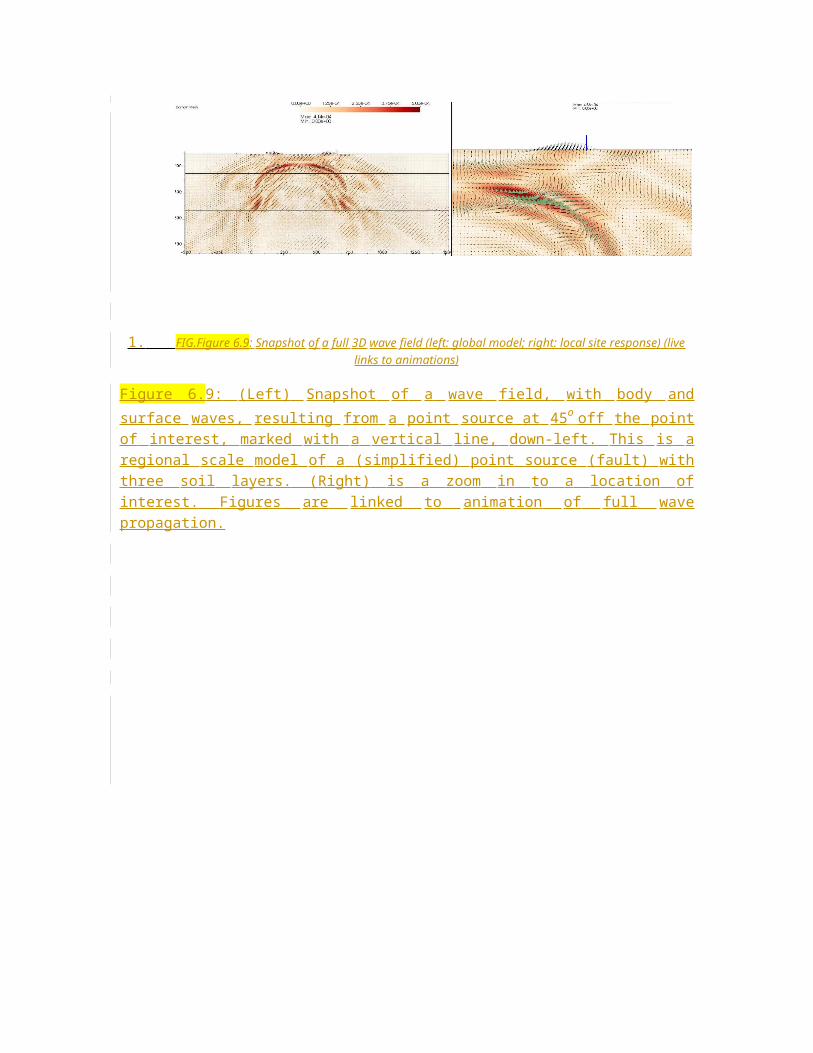
1. FIG.Figure 6.9: Snapshot of a full 3D wave field (left: global model; right: local site response) (live links to animations)

Figure 6.9: (Left) Snapshot of a wave field, with body and surface waves, resulting from a point source at 45o off the point of interest, marked with a vertical line, down-left. This is a regional scale model of a (simplified) point source (fault) with three soil layers. (Right) is a zoom in to a location of interest. Figures are linked to animation of full wave propagation.

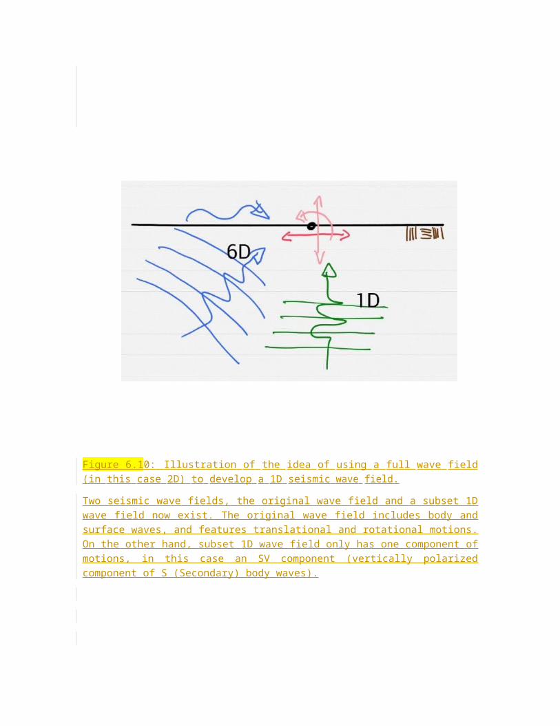
Figure 6.10: Illustration of the idea of using a full wave field (in this case 2D) to develop a 1D seismic wave field.

Two seismic wave fields, the original wave field and a subset 1D wave field now exist. The original wave field includes body and surface waves, and features translational and rotational motions. On the other hand, subset 1D wave field only has one component of motions, in this case an SV component (vertically polarized component of S (Secondary) body waves).

Please note that seismic motions are input in an exact way, using the Domain Reduction Method (Bielak et al., 2003; Yoshimura et al., 2003) (described in chapter 6.4.10) and how there are no waves leaving the model out of DRM element layer (4th layer from side and lower boundaries).

It is also important to note that horizontal motions in one direction at the location of interest (in the middle of the model) are exactly the same for both 2D case and for the 1D case.

Figure 6.12 shows a snapshot of an animation (available through a link within a figure) of difference in response of an NPP excited with full seismic wave field (in this case 2D), and a response of the same NPP to 1D seismic wave field.

2. FIG.Figure 6.11: Left: Snapshot of a full 3D wave field, and Right: Snapshot of a reduced 1D wave field. Wave fields are at the location of interest. Motions from a large scale model were input using DRM, described in chapter 6 (6.4.10). Note body and surface waves in the full wave field (left) and just body waves (vertically propagating) on the right. Also note that horizontal component in both wave fields (left, 2D and right 1D), are exactly the same. Each figure is linked to an animation of the wave propagation.

3. FIG.Figure 6.12: Snapshot of a 3D vs 1D response of an NPP, upper left side is the response of the NPP to full 3D wave field, lower right side is a response of an NPP to 1D wave field.

Figures 6.13 and 6.14 show displacement and acceleration response on top of containment building for both 3D and 1D seismic wave fields.

A number of remarks can be made:

16

Accelerations and displacements (motions, NPP response) of 3D and 1D cases are quite different. In some cases 1D case gives bigger influences, while in other, 3D case gives bigger influences.

Differences are particularly obvious in vertical direction, which are much bigger in 3D case.

Some accelerations of 3D case are larger thanthat those of a 1D case. On the other hand, some displacements of 1D case are larger than those of a 3D case. This just happens to be the case for given source motions (a Ricker wavelet), for given geologic layering and for a given wave speed (and length). There might (will) be cases (combinations of model parameters) where 1D motions model will produce larger influences than 3D motions model, however motions will certainly again be quite different. There will also be cases where 3D motions will produce larger influences than 1D motions. These differences will have to be analyzed on a case by case basis.

In conclusion, response of an NPP will be quite different when realistic 3D seismic motions are used, as opposed to a case when 1D, simplified seismic motions are used. Recent paper, by Abell et al. (2016) shows differences in dynamic behaviour of NPPs same wave fields is used in full 3D, 1D and 3×1D configurations.

17

4. FIG.Figure 6.13: Displacements response on top of a containment building for 3D and 1D seismic input.

18

5. FIG.Figure 6.14: Acceleration response on top of a containment building for 3D and 1D seismic input.

19

1

Real 3D motions (Boris)

SSI models

Structure (Jim) o Stick modelso Plane (2D) modelso 3D modelso Structural properties : Cracked inertia for beams , shear walls, piles

Foundations Foundation modelling is separated into conventional foundation/structure systems (surface founded and shallow embedded), deep foundation (piles), and deeply embedded foundation/structure systems.

Foundation modelling for conventional foundation/structure systemsModelling of surface foundations in a global direct SSI analysis, or in substructure analyses provided the analyses are carried out with the same software for all individual steps, does not pose any difficulty: software like PLAXIS, ABAQUS, GEFDYN, DYNAFLOW, SASSI, CLASSI, MISS3D, Real ESSI, etc.. can account for foundations with any stiffness. In a conventional substructure approach, however, the usual assumption is to consider the foundation as infinitely stiff to define the foundation impedances and the foundation input motion. The question then arises of the validity of this assumption which depends on the relative stiffness of the foundation and of the underlying soil. Stiffness ratios SRv, for the vertical and rocking modes, and SRh

for the horizontal and torsional modes can be introduced to this end. These stiffness ratios depend on the foundations characteristics (axial stiffness EbSb in kN/ml or bending stiffness EbIb in kN.m2/ml) and on the soil shear modulus G or Young’s modulus E. For a circular foundation with diameter B these stiffness ratios are given by

22\* MERGEFORMAT ()

The foundation can be assumed stiff with respect to the soil when:

• SRv > 1 for vertical and rocking modes

• SRh > 5 for horizontal and torsion modes

Usually the condition on SRh is always satisfied. For nuclear reactors and buildings with numerous shear walls the condition on SRv is also satisfied considering the stiffening effect of the walls; for moment resisting frame buildings with a mat foundation, the condition on SRv is hardly satisfied and either a complete analysis taking into account the raft flexibility shall be carried out, or the stiffness of fictitious rigid foundations around the columns shall be computed and specified at each column base, assuming that no coupling exists between the individual footings.

The impedance functions are then introduced in the structural model as springs Kr (real part of the impedance function) and dashpot C related to the imaginary part Ki of the impedance function. Alternatively, the damping ratio of each SSI mode can be computed as

2

33\* MERGEFORMAT ()

The usual practice limits the damping ratio to 30%, but some standards allow for higher values, if properly justified. The main difficulty with the impedance functions is their dependence on frequency, which cannot be easily in considered in time domain analyses or modal spectral analyses. Several possibilities exist to approximately take the frequency dependence into account:

To implement an iterative process which, for each SSI mode, determines the stiffness compatible with the frequency of the corresponding undamped SSI mode; the SSI mode can be identified as the mode with the maximum strain energy stored in the spring.To develop a rheological model which accounts for the frequency dependence by addition of masses connected to the foundation with springs and dashpots(De Barros & Luco 1990, Wolf 1994, Saitoh 2012). The parameters of the rheological are simply determined by curve fitting of the model response to the impedance function. An example of such a model is shown in Figure 8-9 (Pecker 2006).

It should be noted that when the soil profile becomes significantly layered with sharp contrasts in rigidity between layers, the impedances functions become jagged and either of the two procedures described above may become difficult to implement; the only possibility is then to resort to frequency domain solutions.

Finally, if for surface foundations the coupling term between horizontal translation and rocking around the transverse horizontal axis may be neglected, this not true for embedded foundations; in the first instance, the impedance matrix is diagonal and springs and dashpots can be assigned independently to each degree of freedom; in the second one, the impedance matrix contains off–diagonal terms, which makes the rheological model more tricky to develop: if the software does offer the possibility of adding a full stiffness matrix to the foundation, alternatives may consist in connecting the spring at a distance h from the foundation with a rigid beam element (see for instance Kolias et al. 2012).

(a) (b)

0.E+00

2.E+06

4.E+06

6.E+06

8.E+06

1.E+07

0 1 2 3 4 5

Frequency (Hz)

Das

hpot

(MN

-s/m

)

ModelFinite element analysis

-1.E+08

-5.E+07

0.E+00

5.E+07

1.E+08

0 1 2 3 4 5

Frequency (Hz)

Stiff

ness

(MN

/m)

ModelFinite element analysis

3

Figure 8-9: Example of a rheological model and model prediction for the horizontal mode of vibration

The substructure approach, on which the concept of foundation impedances is based, assumes linearity of the system. However, it is well recognized that this is a strong assumption, since non-linearities are present in the soil itself (section 3.2) and at the soil foundation interface (sliding, uplift, section 7.4.6). Soil non-linearities may be partly accounted for by choosing, for the calculation of the impedance matrix, reduced values of the soil properties that reflect the soil nonlinear behaviour in the free field (Section 7.4.4). This implicitly assumes that additional nonlinearities taking place at the soil foundation interface do not affect significantly the overall seismic response.

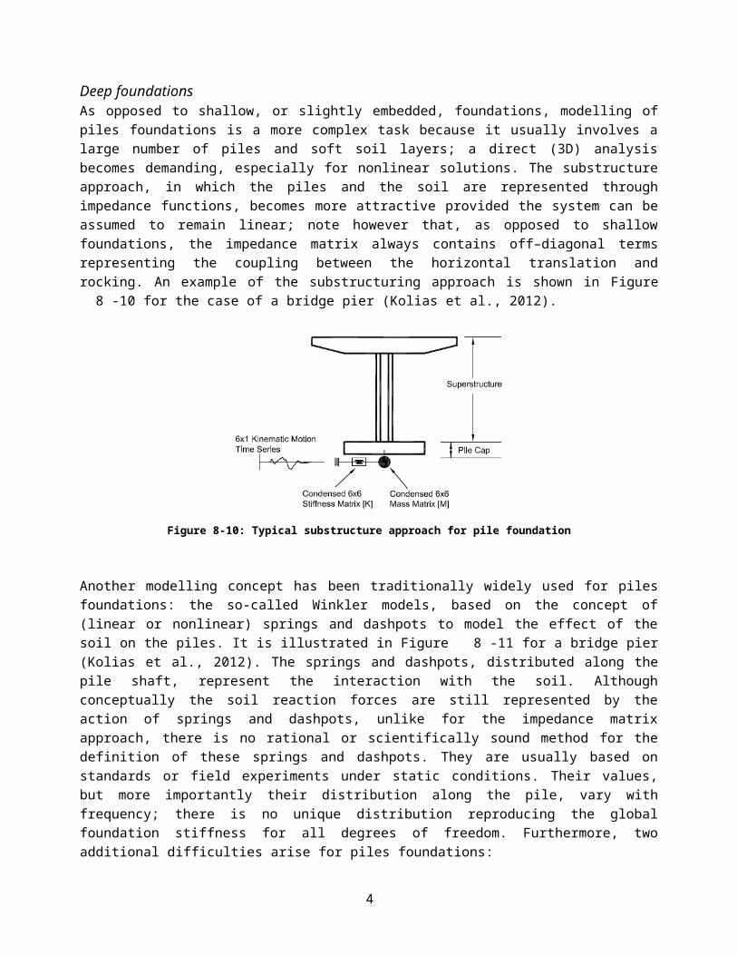
Deep foundationsAs opposed to shallow, or slightly embedded, foundations, modelling of piles foundations is a more complex task because it usually involves a large number of piles and soft soil layers; a direct (3D) analysis becomes demanding, especially for nonlinear solutions. The substructure approach, in which the piles and the soil are represented through impedance functions, becomes more attractive provided the system can be assumed to remain linear; note however that, as opposed to shallow foundations, the impedance matrix always contains off–diagonal terms representing the coupling between the horizontal translation and rocking. An example of the substructuring approach is shown in Figure 8-10 for the case of a bridge pier (Kolias et al., 2012).

Figure 8-10: Typical substructure approach for pile foundation

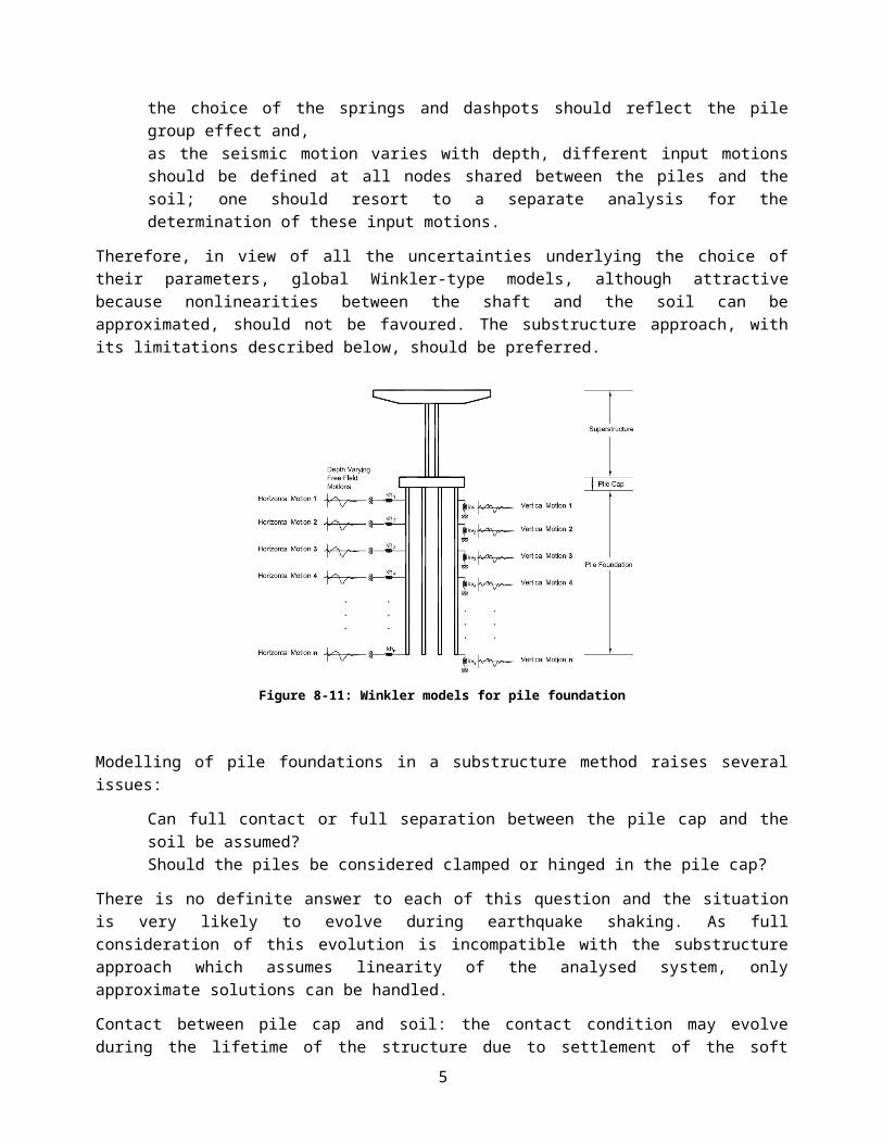
Another modelling concept has been traditionally widely used for piles foundations: the so-called Winkler models, based on the concept of (linear or nonlinear) springs and dashpots to model the effect of the soil on the piles. It is illustrated in Figure 8-11 for a bridge pier (Kolias et al., 2012). The springs and dashpots, distributed along the pile shaft, represent the interaction with the soil. Although conceptually the soil reaction forces are still represented by the action of springs and dashpots, unlike for the impedance matrix approach, there is no rational or scientifically sound method for the definition of these springs and dashpots. They are usually based on standards or field experiments under static conditions. Their values, but more importantly their distribution along the pile, vary with frequency; there is no unique distribution reproducing the global foundation stiffness for all degrees of freedom. Furthermore, two additional difficulties arise for piles foundations:

the choice of the springs and dashpots should reflect the pile group effect and,

4

as the seismic motion varies with depth, different input motions should be defined at all nodes shared between the piles and the soil; one should resort to a separate analysis for the determination of these input motions.

Therefore, in view of all the uncertainties underlying the choice of their parameters, global Winkler-type models, although attractive because nonlinearities between the shaft and the soil can be approximated, should not be favoured. The substructure approach, with its limitations described below, should be preferred.

Figure 8-11: Winkler models for pile foundation

Modelling of pile foundations in a substructure method raises several issues:

Can full contact or full separation between the pile cap and the soil be assumed?Should the piles be considered clamped or hinged in the pile cap?

There is no definite answer to each of this question and the situation is very likely to evolve during earthquake shaking. As full consideration of this evolution is incompatible with the substructure approach which assumes linearity of the analysed system, only approximate solutions can be handled.

Contact between pile cap and soil: the contact condition may evolve during the lifetime of the structure due to settlement of the soft layers caused by consolidation of clayey strata, construction around the existing structure, …. It may also evolve during the earthquake due to soil compaction. Results presented in the appendix for horizontal sway, vertical and rocking impedances show that the impact is negligible for vertical and rocking impedances and is only marginally important for the horizontal impedance. These conclusions apply to pile group with a large number of piles and may be different when few piles are considered. Given the insignificant difference between the two assumptions, it is recommended for design purpose to retain the no contact condition, which is the most likely situation in soft soils.

Fixity at the pile cap connection: during seismic loading the connection may deteriorate and evolve, due to reduction of the connection stiffness, from perfectly clamped piles to a condition where a plastic hinge forms at the connection. The results presented in the appendix compare the dynamic impedances for both extreme conditions: the clamped condition affects the horizontal stiffness but does not affect the vertical

5

or rocking ones. Note however that the reduction in the horizontal stiffness, almost a factor of 2, is certainly much larger than the reduction that would be obtained under the formation of a plastic hinge which, as opposed to the hinged condition, exhibits a residual moment capacity. Regarding the kinematic interaction forces, if the maximum values are not significantly affected, the distribution of the forces along the pile is totally different with maximum values occurring at deeper locations along the pile when the stiffness deteriorates. Based on the obtained results recommendation would be either to run both types of analyses (clamped and hinged connection) and to take the envelope of both conditions, or for a more conservative approach, to take the maximum forces from the hinged analysis and to extend the maximum values upwards to the pile cap connection.

Deeply embedded foundations (SMR)As opposed to shallow or deep foundations, modelling and analysis of deeply embedded structures, like SMRs, are more easily achieved in a global direct time domain or frequency domain analysis. Unless the whole SSI analysis is run within a single software (like SASSI or CLASSI) 0F

1, the conventional substructure approach is not well adapted, although still theoretically possible under the assumption of linear behaviour, because of the large embedment. The embedment creates a strong kinematic interaction between the soil and the structure which significantly alters the freefield motion and develops pressures on the lateral walls. Calculation of these two effects in a conventional substructure approach is complicated and tedious:

Kinematic interaction motion, i.e. the effective foundation input motion, needs to be calculated from a model reflecting the embedment and variation of the freefield motion with depth; furthermore, the true effective input motion contains a rocking component which is not easily applied to the structural model;There is no simple means for evaluating the earth pressures on the outside walls; classical solutions, like the Mononobe and Okabe solution, are not valid for deeply embedded retaining structures that cannot develop an active pressure condition; furthermore, earth pressures and inertia force are likely to be out–of–phase, without any simple solution to easily define the phase shift between both.

Rigorous consideration of these two factors, requires a global finite element model of the embedded part of the structure, and the additional amount of effort to include the structural model is then minimal.

Analyses methods

Dynamic analyses

Substructure methodsSubstructure methods are only valid provided a linear elastic behaviour of all components can be assumed. Therefore, the first task before choosing the analysis method, between a direct method and a substructure method, is to assess this importance of this aspect. However, slight nonlinearities in the soil behaviour can be accepted in the substructure approach and considered, at least in an approximate manner: as indicated in several instances in the TECDOC, reduced soil characteristics can be used in the model; these reduced characteristics represent the strain compatible properties and reflect the soil nonlinearities in the freefield. They are usually calculated from a (1D or 2D) site response analysis (section 8.3.2 and 8.3.3). It is further assumed in the substructure approach that additional nonlinearities that develop due to the interaction 1 It is recalled that SASSI and CLASSI use a substructure approach, but the same software and model are used for the analysis of the soil–foundation substructure and of the structure. Conventional substructure approaches calculate the impedance matrix, simplify it with frequency independent springs and dashpots to be connected to the structural model, which is analyzed with a different software.

6

between the structure and the soil have a second order effect on the overall response; however, they may impact the local response, like for the soil pressures developing along a pile shaft.

The substructure approach has been described in section 7.3 and the successive steps in the approach are illustrated in the flow chart of Figure 8-12; the flowchart, with reference to the boxes numbers in brackets, is detailed below.

Seismological Data [1]

Geotechnical Data [2]

Structural data [3]

RockSpectra [4]

Design soilProfile [5]

Superstructure [8]Ground surface spectraStrain compatible soil characteristics [6]

Foundations [7]

Impedances [10]

KinematicInteraction [9]

FoundationSpectra [13]

KinematicForces [12]

SSI Model [11]

InertialForces [14]

Structural design quantitiesForces, Displacements, Accelerations, FRS [15]

Figure 8-12: Flowchart for the implementation of the substructure approach

Two examples in the appendices illustrate some of the steps ([5], [6], [7], [10], [12], [13], [14], [15]) listed in the flowchart: one example is for an embedded structure and the second one for a piles foundation. They both refer to the conventional substructure approach in which impedances are calculated in a first step and introduced in a structural model.

One example on a deeply embedded structure is developed along the lines of the substructure approach but with all the steps of the SSI analysis run with the same software (SASSI, see note in section 8.4.2.3); therefore, some of the simplifying assumptions of the conventional substructure approach are overcome in this example.

The first step of the analysis starts with the site response analysis to calculate the strain compatible soil characteristics and ground surface response spectra. Site response analyses have been detailed in section 6.3 and 8.3. The input data for this step are:

7

the geotechnical data ([1]) from which a design profile and a constitutive model are chosen for the site (section 3);the seismological data ([2]) from which the rock spectra ([3]) are established either from a probabilistic, or a deterministic, seismic hazard assessment (section 6.4). Time histories representing the rock motion need to be defined following one of the procedures described in section 6.5.

With these data, site response analyses provide the ground surface motion and the strain compatible soil characteristics ([6]). Usually, they are run assuming an equivalent linear constitutive model as illustrated in the examples on embedded foundation and piles foundation in the appendix. Although nonlinear analyses are also possible, the choice of the strain compatible soil properties is less straightforward in this case and requires some amount of judgment.

The second step corresponds to the top right boxes of the flowchart: it establishes from the formwork drawings ([3]) the structural model ([8]) and the foundation model ([9]). As noted in section 8.4.2, the foundation model for the shallow embedded foundation is assumed to correspond to a stiff foundation; the one for the piles foundation of the appendix gathers the piles and the surrounding soil, modelled as continuum media.

With the foundation model and the strain compatible soil characteristics, an impedance matrix is calculated ([10]) and introduced in the structural model with frequency independent values. Section 8.4.2.1 presented two possible alternatives to define the frequency independent impedance matrix. This step produces the SSI model ([11]).

The same foundation model and the surface ground motion are used to calculate the kinematic response of the foundation ([9]); this kinematic response is composed of the foundation input motion ([13]) and of the kinematic forces developed in the foundation ([12]).

The foundation input motion serves as the input to the structural model from which the inertial components of the response are retrieved ([14]).

Finally, the results from the inertial response and from the kinematic response are combined ( [15]) to yield the structural design quantities: forces, accelerations, displacements, Floor Response Spectra. If the kinematic response quantities RK and the inertial response quantities RI are obtained from time history analyses (in time or frequency domains) there is no difficulty in combining, at each time step, their contributions. The total response quantity at any time is given by:

44\* MERGEFORMAT ()

However, in most cases the response quantities are not known as a function of time, and only the maximum inertial response quantities are retrieved from the SSI analyses (for instance when a modal spectral analysis is used). To combine both components, each of them should be alternatively considered as the main action and weighted with a factor 1.0, while the other one is the accompanying action and weighted with a factor :

55\* MERGEFORMAT ()

8

The coefficient depends on how close to each other are the main frequencies leading to the maximum kinematic response quantity and the main frequency leading to the maximum inertial response quantity. The first one is controlled by the SSI mode and the second one by the soil response (fundamental frequency of the soil column). If these two frequencies are well separated, let’s say by 20%, both maxima are uncorrelated in time and their maximum values can be added with the SRSS rule.

66\* MERGEFORMAT ()

If both frequencies are within 20% of each other, it is reasonable to assume that both phenomena are correlated, and the kinematic and inertial response quantities should be added algebraically:

77\* MERGEFORMAT ()

Direct methods: linear, nonlinear (SMR, deep foundations, sliding, uplift (Boris)

Incoherent motions (jim) Freefield SSI

Uncertainties and sensitivity studies

Ground motion (Jim)o Frequency characteristics o Time history representation of ground motiono Spatial variation

Soil It has been pointed in several instances throughout the document that great uncertainties prevail in the soil characteristics due to the difficulty to test soils, to the inherent randomness and spatial variability of soil deposits; uncertainty in soil characteristics is the second, after the ground motion, largest source of uncertainty in SSI analyses. Spatial variability is characterized by correlation distances of the order of a meter in the vertical direction and of some meters in the horizontal one; such small distances preclude a thorough characterization of the deposit. Nevertheless, when enough investigation points are available, stochastic models have been proposed to characterize the spatial variability and used in seismic analyses (Popescu 1995, Popescu et al. 1995, Assimaki et al. 2003). These models remain however seldom used in practice and soil uncertainties are usually handled through sensitivity analyses.

As the constitutive model becomes more complex, the effects of these uncertainties become more and more significant. For the elastic characteristics, it has been recommended to consider at least three velocity profiles corresponding to the best estimate characteristics and to those characteristics divided or multiplied by (1+COV); typically, the coefficient of variation (COV) on the elastic shear wave velocity should not be taken less than 0.25. However, the uncertainty on the elastic properties is not the single parameter that needs to be considered: large uncertainties exist in the determination of the nonlinear shear stress–shear strain curves (or equivalently G/Gmax and damping ratio curves used to define the equivalent linear model); this uncertainty stems from the difficulty to recover undisturbed samples from the ground and to

9

test them in the laboratory; it is therefore essential to compare any measurement to published data to assess its representativeness.

With the use of nonlinear models the number of soil parameters to define increases and therefore so does the uncertainty in the prediction of the soil response. Furthermore, there is a large variety of nonlinear models in the technical literature and none of them can be considered as the best model; the choice of the constitutive model, and the control and ability of the analyst, therefore contributes to the overall uncertainty. To cover this aspect, the use of preferably 2 nonlinear constitutive models, run by 2 different analysts has been recommended.

Structure (Jim)o Stiffness of elements (cracked inertia)o Eccentricity

Soil-foundation-structure models (Boris)o Modelling of partial embedment o Modelling of sliding, uplift, gaps (piles)o Modelling of incompressibilityo Structure-soil-structure interaction

10

1 Introduction

Investigations of SSI have shown that the dynamic response of a structure supported on elastic-plastic soil may differ significantly from the response of the same structure when supported on a rigid base Chopra & Gutierrez (1974), Bielak (1978). The difference comes from dissipation of part of the vibrational energy by hysteresis action of the soil or structure itself. Jeremic´ et al. (2004) found that SSI can have detrimental effects on structural behavior and that that dependents on three components, namely the dynamic character- istics of the earthquake motion, the foundation soil and the structure. Hence dynamics of structures is really a problem of Earthquake Soil Structure Interaction (ESSI).

Dissipation of energy during seismic events is another important factor to consider in design for its safety and economy. Dissipating energy in structure can lead to material degradation and damage. It is desired to dissipate most of the energy in soil with acceptable level of deformations in structure. Proper modeling of energy dissipation (Yang et al., 2017) can be used to optimize soil structure systems for safety and economy.

Presented in this example is a linear elastic and an inelastic analysis of a complete, detailed model of an

NPP, subjected to full 3D seismic wave field. Example is based on Sinha et al. (2017).It is noted that input files for these models are available at this LINK, and can be directly simulated

using Real ESSI Simulator (http://real-essi.us/), that is available on Amazon Web Services (https://aws.amazon.com/).

2 Model Development and Simulation Details

The Nuclear Power Plant (NPP) modeled here is a symmetric structure with shallow foundation of thickness3.5m and size 100m. Figure 1a shows a slice view of the model in normal y direction (perpendicular to plane of the paper). Solid brick elements were used to model soil and foundation. The NPP structure was modelled by elastic shell elements. Material parameters for soil, contact and the structure are given by Sinha et al. (2017)

2.1 Structural Model

The NPP structural model consists of auxiliary building, containment building and shallow foundation as shown in Figure 1b. The auxiliary building consists of 4 floors of 0.6m thickness, ceiling floor of 1m thickness, exterior wall of 1.6m thickness and interior walls of 0.4m thickness. The exterior and interior walls are embedded down to the depth of the foundation. The containment building is a cylinder of diameter20m and height 40m with wall thickness of 1.6m. There is a gap of 0.2m between the containment and auxiliary building. Top of the containment building is covered by semi-spherical dome of radius 20m. The foundation is square shallow footing of size 100m and thickness 3.5m. The containment building and the auxiliary building were modelled as shell elements and foundation as linear brick elements.

11

AuxiliaryBuilding

ContainmentBuilding

DampingLayers

Center ofESSI Box

Contact

Soil

DRM Layer

Foundation

DampingLayers

(a) Finite Element Model (b) Auxiliary And Containment Building

Figure 1: Nuclear power plant model with shallow foundation.

2.2 Soil Model

The depth of the soil modelled below the foundation is 120 m, representing also the depth of DRM layer. It is assumed that within this range the soil can behave inelasticaly. The soil is assumed to be a stiff saturated- clay with undrained behavior. shear velocity of 500 m/s, unit weight of 21.4 kP a and Poisson’s ratio of 0.25. To represent the travelling wave accurately for a given frequency, 10 8 node brick or 3 27 node brick elements are required (Watanabe et al., 2016). Seismic waves are analyzed up to fmax = 10Hz. The smallest wavelength λmin to be captured thus, can be estimated as

λmin = v/fmax (1)

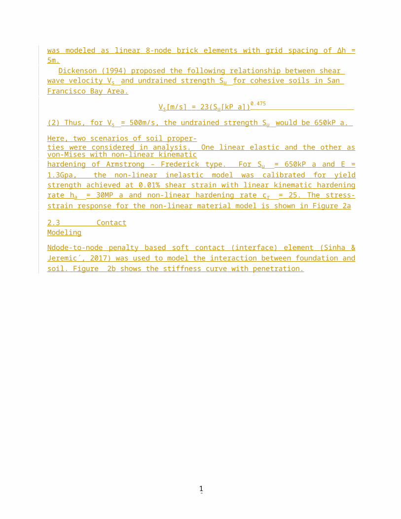
where, v is the smallest shear wave velocity of interest. For v = 500m/s and fmax = 10Hz the minimum wavelength λmin would be (500m/s)(10/s) = 50m. Choosing 10 nodes/elements per wavelength the element size would be 5m. Jeremic´ et al. (2009), Watanabe et al. (2016) state that even by choosing mesh size ∆h = λmin/10, smallest wavelength that can be captured with confidence is λ = 2∆h i.e. a frequency corresponding to 5fmax . Based on the above analysis, soil was modeled as linear 8-node brick elements with grid spacing of ∆h = 5m.

Dickenson (1994) proposed the following relationship between shear wave velocity Vs and undrained strength Su for cohesive soils in San Francisco Bay Area.

Vs[m/s] = 23(Su[kP a])0.475

(2) Thus,

for Vs = 500m/s, the undrained strength Su would be 650kP a. Here, two scenarios of soil proper-ties were considered in analysis. One linear elastic and the other as von-Mises with non-linear kinematichardening of Armstrong – Frederick type. For Su = 650kP a and E = 1.3Gpa, the non-linear inelastic model was calibrated for yield strength achieved at 0.01% shear strain with linear kinematic hardening rate ha = 30MP a and non-linear hardening rate cr = 25. The stress-strain response for the non-linear material model is shown in Figure 2a

2.3 Contact Modeling

12

Ndode-to-node penalty based soft contact (interface) element (Sinha & Jeremic´, 2017) was used to model the interaction between foundation and soil. Figure 2b shows the stiffness curve with penetration.

13

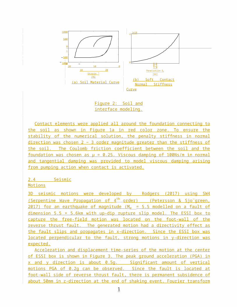
10002 1e10

500

0 1

500

100020 10 0 10 20

Strain ² [%]

(a) Soil Material Curve

00.0 0.5 1.0

Penetration δ n [mm]

(b) Soft Contact Normal StiffnessCurve

Figure 2: Soil and interface modeling.

Contact elements were applied all around the foundation connecting to the soil as shown in Figure 1a in red color zone. To ensure the stability of the numerical solution, the penalty stiffness in normal direction was chosen 2 − 3 order magnitude greater than the stiffness of the soil. The Coulomb friction coefficient between the soil and the foundation was chosen as µ = 0.25. Viscous damping of 100Ns/m in normal and tangential damping was provided to model viscous damping arising from pumping action when contact is activated.

2.4 Seismic Motions

3D seismic motions were developed by Rodgers (2017) using SW4 (Serpentine Wave Propagation of 4th

order) (Petersson & Sjo¨green, 2017) for an earthquake of magnitude (Mw = 5.5 modelled on a fault of dimension 5.5 × 5.6km with up-dip rupture slip model. The ESSI box to capture the free-field motion was located on the foot-wall of the reverse thrust fault. The generated motion had a directivity effect as the fault slips and propagates in x-direction. Since the ESSI box was located perpendicular to the fault, strong motions in y-direction was expected.

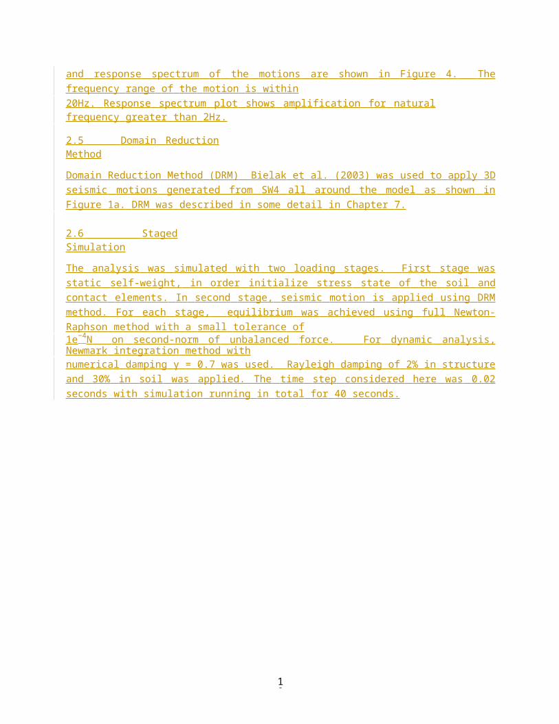
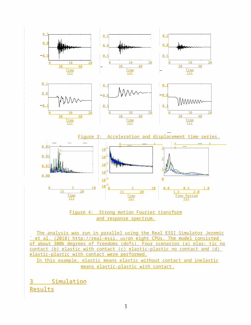
Acceleration and displacement time-series of the motion at the center of ESSI box is shown in Figure 3. The peak ground acceleration (PGA) in x and y direction is about 0.5g. Significant amount of vertical motions PGA of 0.2g can be observed. Since the fault is located at foot-wall side of reverse thrust fault, there is permanent subsidence of about 50mm in z-direction at the end of shaking event. Fourier transform and response spectrum of the motions are shown in Figure 4. The frequency range of the motion is within20Hz. Response spectrum plot shows amplification for natural frequency greater than 2Hz.

2.5 Domain Reduction Method

Domain Reduction Method (DRM) Bielak et al. (2003) was used to apply 3D seismic motions generated from SW4 all around the model as shown in Figure 1a. DRM was described in some detail in Chapter 7.

2.6 Staged Simulation

The analysis was simulated with two loading stages. First stage was static self-weight, in order initialize stress state of the soil and contact elements. In second stage, seismic motion is applied using DRM method. For each stage, equilibrium was achieved using full Newton-Raphson method with a small tolerance of1e−4 N on second-norm of unbalanced force. For dynamic analysis, Newmark integration method with

14

numerical damping γ = 0.7 was used. Rayleigh damping of 2% in structure and 30% in soil was applied. The time step considered here was 0.02 seconds with simulation running in total for 40 seconds.

15

0.5

0.0

0.5

0.0

0.5

0.0

0.5

0 10 20 30 40Time [s]

0.5

0 10 20 30 40Time [s]

0.5

0 10 20 30 40Time [s]

0.1 0.1 0.1

0.0 0.0 0.0

0.1

0 10 20 30 40Time [s]

0.1

0 10 20 30 40Time [s]

0.1

0 10 20 30 40Time [s]

Figure 3: Acceleration and displacement time series.

0.03

0.02

0.01

0.00

x y z10-1

10-2

10-3

10-4

10-5

10-6

x y z3

2

1

0

x y z

0 5 10 15 20Time [s]

0 5 10 15 20Time [s]

0.0 0.5 1.0 1.5 2.0Time Period [s]

Figure 4: Strong motion Fourier transform and response spectrum.

The analysis was run in parallel using the Real ESSI Simulator Jeremic´ et al. (2018) http://real-essi. us/on eight CPUs. The model consisted of about 300k degrees of freedoms (dofs). Four scenarios (a) elas- tic no contact (b) elastic with contact (c) elastic-plastic no contact and (d) elastic-plastic with contact were performed.

In this example, elastic means elastic without contact and inelastic means elastic-plastic with contact.

3 Simulation Results

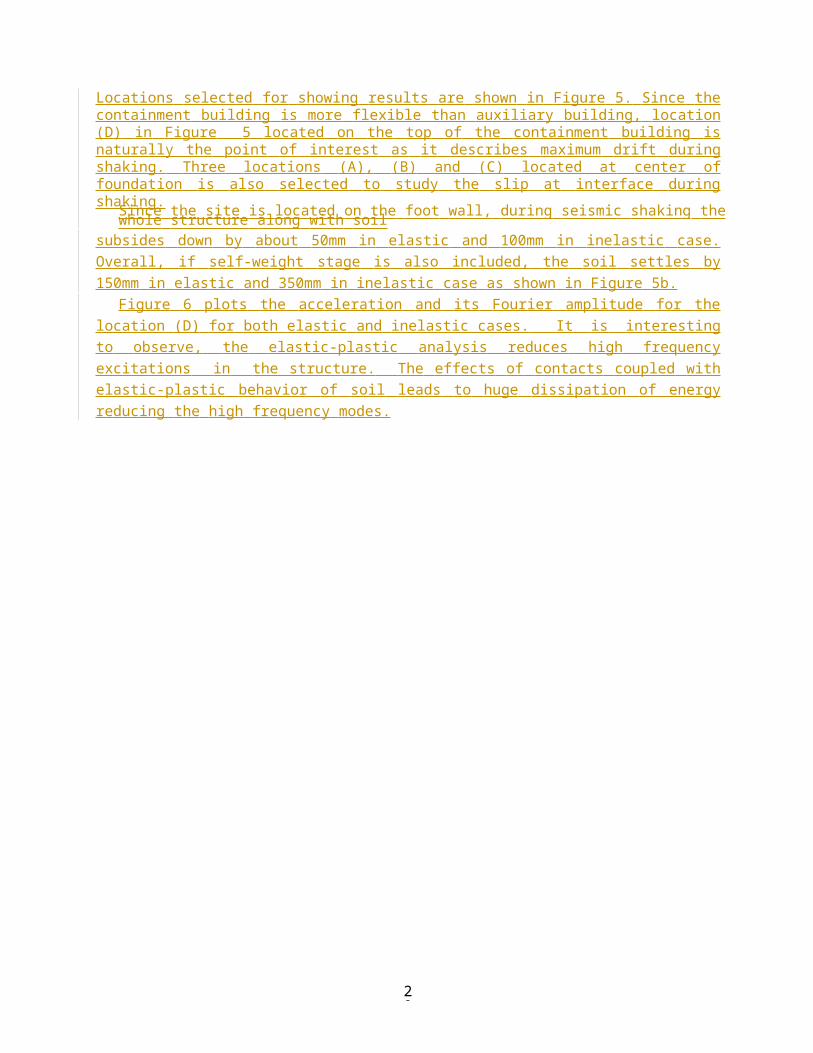
Locations selected for showing results are shown in Figure 5. Since the containment building is more flexible than auxiliary building, location (D) in Figure 5 located on the top of the containment building is naturally the point of interest as it describes maximum drift during shaking. Three locations (A), (B) and (C) located at center of foundation is also selected to study the slip at interface during shaking.

Since the site is located on the foot wall, during seismic shaking the whole structure along with soil subsides down by about 50mm in elastic and 100mm in inelastic case. Overall, if self-weight stage is also included, the soil settles by 150mm in elastic and 350mm in inelastic case as shown in Figure 5b.

Figure 6 plots the acceleration and its Fourier amplitude for the location (D) for both elastic and inelastic cases. It is interesting to observe, the elastic-plastic analysis reduces high frequency

16

excitations in the structure. The effects of contacts coupled with elastic-plastic behavior of soil leads to huge dissipation of energy reducing the high frequency modes.

17

D Elastic Inelastic

0.1

0.2

0.3

A B C

(a) Selected Locations

0.4 0 10 20 30 40

Time [s]

(b) Total Displacement

Figure 5: Locations selected to study non-linear effects and plot of total displacement at center of modelElastic (elastic with contact) and Inelastic (Elastic-Plastic with contact).

Elastic Inelastic

1

0

Elastic Inelastic

1

0

Elastic Inelastic

1

0

10 10 20 30 40

Time [s]

10 10 20 30 40

Time [s]

(a) Acceleration

10 10 20 30 40

Time [s]

0.10

0.05

Elastic Inelastic

0.10

0.05

Elastic Inelastic0.10

0.05

Elastic Inelastic

0.00 0 5 10 15 20Frequency [Hz]

0.00 0 5 10 15 20Frequency [Hz]

(b) Fourier Amplitude of Acceleration

0.00 0 5 10 15 20Frequency [Hz]

Figure 6: Seismic response at top of containment building Elastic (elastic without contact) and Inelastic(elastic-plastic with contact).

The introduction of contact can result in opening and closing of gaps at the soil-foundation interface for stronger earthquakes. However, here for the considered seismic motion for both elastic and inelastic case with contact, no uplift was observed. Analysis of different structures done previously Jeremic´ et al. (2013) showed gap opening and closing during seismic shaking.l Figure 7 shows the relative displacement of NPP structure for elastic and inelastic analysis at 11 seconds. In elastic case, the structure drifts while the deformation in soil remains small. In the inelastic case, the soil deforms and plastify keeping the structure deformation small. The elasto-plastic soil acts as a natural base isolator.

Figure 8 shows slip of foundation with respect to soil at location (A), (B) and (C) for elastic soil with contact and elastic-plastic soil with contact.

18

Elastic With Contact Elastic-Plastic With Contact

Figure 7: Deformation of the NPP structure at 11 seconds (scaled 100 times).Elastic Inelastic

40

20

0

20

40

Elastic Inelastic40

20

0

20

40

Elastic Inelastic40

20

0

20

400 10 20 30 40Time [s]

0 10 20 30 40Time [s]

(a) Slip in x-direction

0 10 20 30 40Time [s]

Elastic Inelastic40

20

0

20

40

Elastic Inelastic40

20

0

20

40

Elastic Inelastic40

20

0

20

400 10 20 30 40Time [s]

0 10 20 30 40Time [s]

(b) Slip in y-direction

0 10 20 30 40Time [s]

Figure 8: Slip of foundation with respect to soil beneath it in x-y slice plane for Elastic (elastic with contact)and Inelastic (Elastic-Plastic with contact).

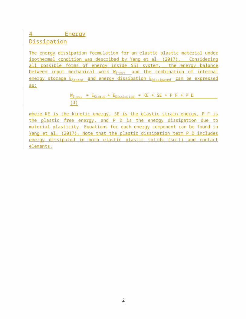
4 Energy Dissipation

The energy dissipation formulation for an elastic plastic material under isothermal condition was described by Yang et al. (2017). Considering all possible forms of energy inside SSI system, the energy balance between input mechanical work WInput and the combination of internal energy storage EStored and energy dissipation EDissipated can be expressed as:

W Input = E Stored + E Dissipated = KE + SE + P F + P D (3)

where KE is the kinetic energy, SE is the elastic strain energy, P F is the plastic free energy, and P D is the energy dissipation due to material plasticity. Equations for each energy component can be found in Yang

19

et al. (2017). Note that the plastic dissipation term P D includes energy dissipated in both elastic plastic solids (soil) and contact elements.

20

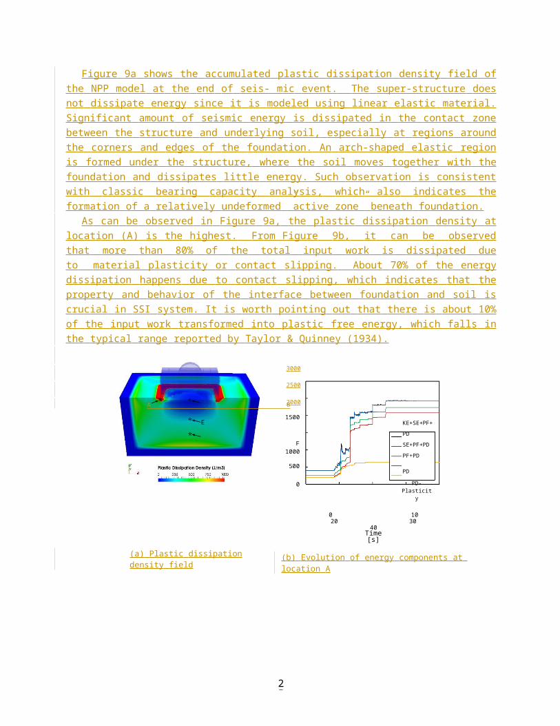
Figure 9a shows the accumulated plastic dissipation density field of the NPP model at the end of seis- mic event. The super-structure does not dissipate energy since it is modeled using linear elastic material. Significant amount of seismic energy is dissipated in the contact zone between the structure and underlying soil, especially at regions around the corners and edges of the foundation. An arch-shaped elastic region is formed under the structure, where the soil moves together with the foundation and dissipates little energy. Such observation is consistent with classic bearing capacity analysis, which also indicates the formation of a relatively undeformed ”active zone” beneath foundation.

As can be observed in Figure 9a, the plastic dissipation density at location (A) is the highest. From Figure 9b, it can be observed that more than 80% of the total input work is dissipated due to material plasticity or contact slipping. About 70% of the energy dissipation happens due to contact slipping, which indicates that the property and behavior of the interface between foundation and soil is crucial in SSI system. It is worth pointing out that there is about 10% of the input work transformed into plastic free energy, which falls in the typical range reported by Taylor & Quinney (1934).

3000

2500

2000A B

1500E

F 1000

500

0

KE+SE+PF+PD

SE+PF+PD

PF+PD

PD

PD-Plasticity

0 10 20 30 40Time [s]

(a) Plastic dissipation density field (b) Evolution of energy components at location A

21

Figure 9: Energy dissipation in SMR model for inelastic (elastic-plastic soil with contact).

22

Verification an n d validation of models (Boris)

1 IntroductionInelastic analysis of earthquake soil structure interaction (ESSI) behavior requires expertise in a number of areas. For example, knowledge of soil and rock mechanics is necessary for proper modeling of dry, partially or fully saturated soil and rock domain under a structure. Interface between structural foundations and the soil/rock beneath is modeled using (soft) contact ele- ments, that can also be dry or saturated. Modeling of structure, made of concrete and/or steel, requires knowledge of structural mechanics. Modeling of systems and components (SCs) within structure can also be done with tne same large scale modeling endeavor, although such SCs can also be modeled separately, de-coupled as they might not contribute in any significant way to ESSI of the system. Earthquake motion modeling, that are used for ESSI analysis, represents a very important component of overall modeling approach.

Equally important is the numerical simulation approach used to develop numerical results using above developed models. Different finite elements with a variety of mass, damping and stiffness matrices, different numerical algorithms for constitutive and global solution advancement, and different finite element meshes will influence results.

Presented here is a step by step, hierarchical approach to modeling and simulation of earth- quake soil structure interaction (ESSI) for a generic concrete building. Approach is based on reliance on numerical modeling and simulation expertise as well as on sound engineering judg- ment.

Input files for all the examples from this section are available online at this LINK. All the examples can run directly at the Amazon Web Services (AWS), using RealESSISimulator, through Real ESSI image that is available on AWS.

45m5m 10m

30m

65m 3x20

m5m

23

2 Inelastic, Nonlinear, Hierarchical Analysis Steps

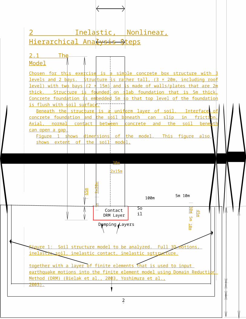
2.1 The Model

Chosen for this exercise is a simple concrete box structure with 3 levels and 2 bays. Structure is rather tall, (3 × 20m, including roof level) with two bays (2 × 15m) and is made of walls/plates that are 2m thick. Structure is founded on slab foundation that is 5m thick. Concrete foundation is embedded 5m so that top level of the foundation is flush with soil surface.

Beneath the structure is a uniform layer of soil. Interface of concrete foundation and the soil beneath can slip in friction. Axial, normal contact between concrete and the soil beneath can open a gap.

Figure 1 shows dimensions of the model. This figure also shows extent of the soil model,

30m

2x15m

ContactDRM Layer

Damping Layers

Soil

100m 5m 10m

Figure 1: Soil structure model to be analyzed. Full 3D motions, inelastic soil, inelastic contact, inelastic sgtsructure.

together with a layer of finite elements that is used to input earthquake motions into the finite element model using Domain Reduction Method (DRM) (Bielak et al., 2003, Yoshimura et al.,2003).

Earthquake motions are characterized by body waves that propagate from the source. Body waves interacting with the surface create surface waves. Both body and surface earthquake waves will excite motions in the soil structure system.

All the models presented are available online. Models can be updated, materials changes, and material parameters updated by the end users. All the models can be analyzed using the Real ESSI Simulator (http://real-essi.us/) that is available on Amazon Web Services (https://aws.amazon.com/).

5

Figure 2: Finite element mesh of the full model.

Figure 3: Soil structure model to be analyzed. Cut through the full model, showing finite element mesh on a deformed model.

6

2.2 Free Field 1D

First step in model development is the 1D wave propagation analysis. Figure 4 shows a 1D mode wave propagation model. The model is made up with 3D brick finite elements, that are constrained with boundary conditions so that only 1D shear waves, polarized in vertical plane, hence SV waves, can propagate. A presence of the DRM layer in the model shown in Figure 4,

Figure 4: 1D wave propagation simulation model.

as well as two layers of finite elements outside of the DRM layer, that are used to support the model.Seismic motions used for this 1D analysis are obtained from one component of a full 3D

seismic motions at the surface. Surface motions are then deconvoluted to the DRM layer, and are used to develop DRM forces.

Elastic Material. Analysis of 1D wave propagation using elastic material is first performed.Results obtained with linear elastic material using Real ESSI Simulator can be compared using analytic

1D wave propagation solution for elastic material. Such analytic solutions are available in books (Kramer, 1996, Semblat & Pecker, 2009, Kausel, 2006, 2017), and are also implemented in a number of available programs, such as SHAKE (Idriss & Sun, 1992).

Input files for this models are available at this LINK, and can be directly simulated using RealESSI Simulator (http://real-essi.us/), that is available on Amazon Web Services (https://aws.amazon.com/).

Elastoplastic Material. Elastic plastic analysis of 1D wave propagation can be accomplished on the very same 1D model, as described in a section above.

Figure 5 shows results at the top of 1D soil column. Response spectrum of motion is shown in Fig. 6.

Acce

lera

tion

[m/s

^2]

Pseu

do-S

pect

ral A

ccel

erati

on S

a [g

]

Spec

tral

Dis

plac

emen

t [m

]Ac

cele

ratio

n [m

/s^2

]

7

4 Time Series of Acceleration

Soil Bottom Motion

3 Soil Top Motion

2

0.30

0.25

FFT of Acceleration

Soil Bottom Motion

Soil Top Motion

1 0.20

0

0.151

2 0.10

3

0.0545 0 1 2 3 4 5 6 7 8 9

Time [s]0.0010-1

100

101

Frequency [Hz]

Figure 5: 1D, elastic-plastic results for the top of soil column.

1.4 Pseudo-Spectral Acceleration 0.05 Spectral Displacement

1.2

0.04

1.0

0.80.03

0.60.02

0.4

0.20.01

0.010-1

100

101

102

Frequency [Hz]0.00 10-1

100

101

102

Frequency [Hz]

Figure 6: Simulation results: response spectrum at the top of soil.

8

Deformed shape of a 1D wave propagating through the model, at particular time instance, is shown in Figure ??. It is noted that a DRM layer, single finite element in this case, is significantly deformed, as that layer is used to input seismic motions into the model.

Figure 7: 2 Simulation model.

Input files for this models are available at this LINK, and can be directly simulated using RealESSI Simulator (http://real-essi.us/), that is available on Amazon Web Services (https:

//aws.amazon.com/).

9

2.3 Free Field 3D

The very same seismic wave field that is used the previous 1D example, is used for input in the full 3D finite element model, shown in Figure 8.

Figure 8: 3D simulation model for free field wave propagation modeling.

Although finite element model is full 3D, since the seismic wave field input is 1D, only 1Dwave is expected to propagate, and results should be very similar to the 1D model results.

Two sets of material parameters are used, linear elastic and elastic-plastic.

Elastic Material. Input files for this models are available at this LINK, and can be directly simulated using Real ESSI Simulator (http://real-essi.us/), that is available on Amazon Web Services (https://aws.amazon.com/).

Elastic-Plastic Material. Inelastic, nonlinear, elastic-plastic material parameters, are given for von Mises material model with nonlinear kinematic hardening of Armstrong Frederic type, same as material model used for the 1D model.

It is important to note that material models for 1D and 3D cases are exactly the same. The difference between 1D and 3D models is in model geometry and boundary conditions.

The time series of top surface accelerations and spectra displacements are are shown in Fig. 9.

Acce

lera

tion

[m/s

^2]

Acce

lera

tion

[m/s

^2]

10

Time Series of Acceleration

Soil Bottom Motion4 Soil Top Motion

0.35

0.30

FFT of Acceleration

Soil Bottom Motion

Soil Top Motion

2 0.25

0.20

0

0.15

2 0.10

0.054

0 1 2 3 4 5 6 7 8 9Time [s]

0.0010-1

100

101

Frequency [Hz]

Figure 9: Simulation results: acceleration time series.

Pseu

do-S

pect

ral A

ccel

erati

on S

a [g

]

Spec

tral

Dis

plac

emen

t [m

]

11

The response spectra of top surface motion are shown in Fig. 10.

1.4 Pseudo-Spectral Acceleration 0.06 Spectral Displacement

1.20.05

1.00.04

0.8

0.60.03

0.40.02

0.2 0.01

0.010-1

100

101

102

Frequency [Hz]0.00 10-1

100

101

102

Frequency [Hz]

Figure 10: Simulation results: response spectrum at soil top.

Deformed shape at a particular time step is shown Fig. 11.

Figure 11: 4 Simulation model.

Input files for this models are available at this LINK, and can be directly simulated using RealESSI Simulator (http://real-essi.us/), that is available on Amazon Web Services (https:

//aws.amazon.com/).

12

2.4 Soil-Foundation Interaction 3D

After 1D annd 3D free field motions are developed, using first linear elastic and then inelastic material models, next step is to add a foundation. The idea is that by adding just a foundation and not a complete foundation-structure system, model is not significantly changed from previous free field model. Hence, response of the soil foundation system should be similar to the free field response.

Elastic Material. Initial analysis is using linear elastic model, for soil, for foundation, for the contact zone, as well as for the structure. Analysis begins with very small motions, in 1D and then extends to 3D motions, both of which are described later.

Input files for this models are available at this LINK, and can be directly simulated using RealESSI Simulator (http://real-essi.us/), that is available on Amazon Web Services (https://aws.amazon.com/).

Inelastic Material Model, von-Mises Armstrong-Frederick or von-Mises G/Gmax Material or Drucker-Prager Armstrong-Frederick or Drucker-Prager G/Gmax Material. Analysis using in- elastic, nonlinear soil material begins with very small motions. It is expected that such very small motions, will produce essentially linear elastic response that should be comparable and very close to linear elastic response.

It should be noted that depending on complexity of soil behavior and on available test data, different material models can be used for modeling soil, as discussed in Chapter 3. For pressure insensitive material behavior (total stress analysis for example, von Mises based material models are used. When mean stress (mean confining pressure/stress) is important, pressure sensitive models need to be used, that are based on versions of Drucker Prager yield surface.

Contact Elements. In addition to inelastic behavior of soil, modeled using elastic-plastic material models for soil solids, contact zone, between foundations and adjacent soil/rock significantly contributes to the inelastic/nonlinear behavior of the ESSI system.

Addition of contact elements to the ESSI model requires further model verification, as was done for addition of inelastic/elastic-plastic models. It is recommended that contact elements be initially added to a model where all other components are linear elastic. ESSI model with contact elements is initially tested with using very small motions so that contact is not expected to open a gap or slip. Response with no slip can achieved by prescribing large friction angle, that is used only to prevent slop. No gap condition cannot be insured, even if the first loading stage if self weight, since some gaps might open during self weight, however large or small friction angle is used. Another option for initial testing is to apply sticky condition to contact elements, where plastic slip or gap opening is prevented by contact model implementation.

Once contact elements are verified for very small forces and motions, more realistic material parameters should be used. For frictional behavior, elastic – perfectly plastic, or elastic – hardening plastic or elastic – hardening-softening contact constitutive law should be chosen based on contact behavior test data. Axial contact behavior for concrete and soil/rock is best modeled using soft contact, where axial stress-strain response is a nonlinear function, as described in chapter 7.

45m

5m

10m

5m

13

Inelastic Soil Material Model and Inelastic Contact Once both inelastic, elastic-plastic modeling of soil (solids) and contact is verified separately, inelastic models for soil and contact can be introduced into the finite element model. Again, very small motions or forces should be used initially, with expectation of an elastic. Increase in demand (forces or motions) should result in yielding of elastic-plastic soil and contacts. Inelastic response results in reduction of frequencies and dynamic motions, with a potential increase in permanent deformation after shaking.

100m 40m 100m 5

m 10m

ContactSoil

DRM Layer

Damping Layers

Figure 12: 5 Simulation model.

Results of the simulation are shown in Fig. 22.

Figure 13: Soil foundation interaction results.

Input files for all the models in this section are available at this LINK, and can be directly simulated using Real ESSI Simulator (http://real-essi.us/), that is available on Amazon Web Services (https://aws.amazon.com/).

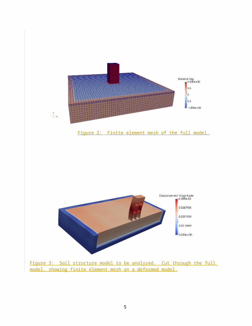
65m

5m

3x20

m

14

2.5 Analysis of a Structure Alone

In order to verify structural model, it is useful to separate structural model from the soil and analyze fixed based model.

2.5.1 Eigen Analysis

Eigen analysis of a fixed base structural model should provide a good check of the structural model, natural (eigen) frequencies, and natural (eigen) modes.

30m

2x15m

Figure 14: Structure on a fixed based simulation model.

For this particular example, eigen modes and frequencies are given in Figures 15 and 16

Figure 15: Eigen frequencies: f1 = 3.473873Hz f2 = 3.473873Hz f3 = 6.877667Hz (eigen mode1 to 3 from left to right).

65m

5m

3x20

m

15

Figure 16: Eigen frequencies: f4 = 11.500571Hz f5 = 11.500571Hz f6 = 12.133523Hz (eigen modes 4 to 6 from left to right).

Input files for eigen analysis of the fixed base structure are available at this LINK, and can be directly simulated using Real ESSI Simulator (http://real-essi.us/), that is available on Amazon Web Services (https://aws.amazon.com/).

2.5.2 Imposed Motion

In addition to eigen analysis, fixed base structural model is used to test response of a fixed base structure. This is important as it provides an opportunity to compare results between different finite element programs, some of which can only model dynamics of fixed base structures.l

Fixed based structural model is shown in Figure 17 while deformation during imposed motions at the base, at one particular time instance, is shown in Figure 18.

30m

2x15m

Figure 17: Fiexed base structural model with motions imposed at the base.

Acce

lera

tion

[m/s

^2]

Acce

lera

tion

[m/s

^2]

16

Figure 18: Fixed base structural model, deformation shape during imposed motions at the base.

6 Time Series of Acceleration

Structural Top Motion

0.30 FFT of Acceleration

Structural Top Motion

Foundation Bottom Motion

4 0.25Foundation Bottom Motion

2 0.20

0 0.15

2 0.10

4 0.05

60 1 2 3 4 5 6 7 8 9Time [s]

0.0010-1

100

101

Frequency [Hz]

Figure 19: Simulation Results: Acceleration Time Series with 1D imposed motion.

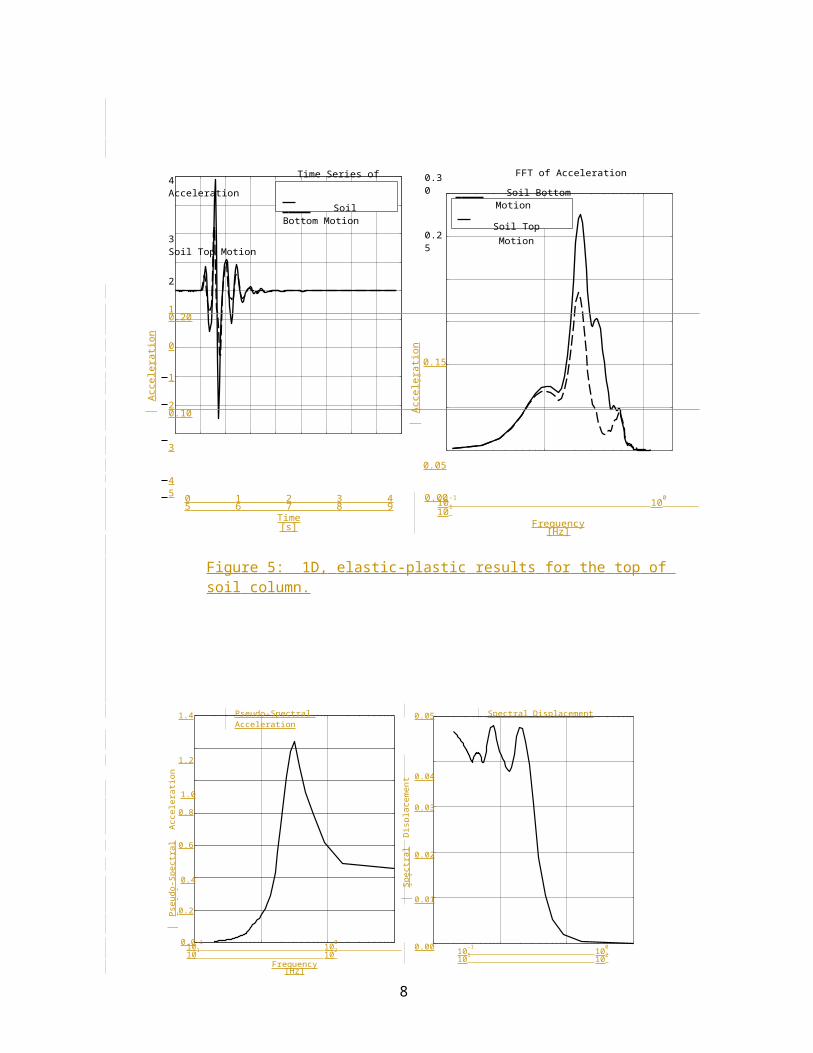
Pseu

do-S

pect

ral A

ccel

erati

on S

a [g

]Ps

eudo

-Spe

ctra

l Acc

eler

ation

Sa

[g]

Spec

tral

Dis

plac

emen

t [m

]Sp

ectr

al D

ispl

acem

ent [

m]

17

The time series of simulation results is shown in Fig. 19. The response spectrum of motion is shown in Fig. 20.

0.16 Pseudo-Spectral Acceleration 0.0030 Spectral Displacement

0.14

0.0025

0.12

0.10 0.0020

0.08 0.0015

0.06

0.0010

0.04

0.020.0005

0.00 10-1

100

101

102

Frequency [Hz]0.0000 10-1

100

101

102

Frequency [Hz]

0.16 Pseudo-Spectral Acceleration 0.0030 Spectral Displacement

0.14

0.0025

0.12

0.10 0.0020

0.08 0.0015

0.06

0.0010

0.04

0.020.0005

0.00 0 1 2 3 4 5Period [s]

0.0000 0 1 2 3 4 5Period [s]

Figure 20: Simulation Results: Response Spectrum of Structure Top with 1D imposed motion.

Input files for eigen analysis of the fixed base structure are available at this LINK, and can be directly simulated using Real ESSI Simulator (http://real-essi.us/), that is available on Amazon Web Services (https://aws.amazon.com/).

18

2.6 3D Soil-Structure Interaction

Much like in the case of soil and the foundation alone, full earthquake soil structure interaction (ESSI), with complete model for soil, contacts, foundation and the structure, starts, with very small forcing and small motions, expecting essentially linear elastic response.

Elastic Material. Elastic material applies to all components of the system including the soil, contacts (no slip or gapping), foundation and the structure.

Inelastic Soil and Inelastic Contact Model. Inelastic soil modeling uses any of the models that are appropriate, as discussed in section on soil modeling in chapters 4 and 7 as well as in this chapter.

It is important to note that initially, due to small shakes and/or forcing, elastic response is expected. With the increase in amplitude of forcing and/or shaking, development of nonlinear response is expected, in both soil and the contact zone.

Inelastic, Nonlinear Concrete Structure. Results of the simulation are shown in Fig. 22.

Simulation using 1D motions. The time series of simulation results is shown in Fig. 23.The response spectrum of motion is shown in Fig. 24. Input files for all 3D ESSI models, using 1D seismic motions are are available at this LINK, and

can be directly simulated using Real ESSI Simulator (http://real-essi.us/), that is available on Amazon Web Services (https://aws.amazon.com/).

Simulation using 3D motions. The time series of simulation results is shown in Fig. 25.The response spectrum of motion is shown in Fig. 26.Input files for all 3D ESSI models, using 1D seismic motions are are available at this LINK, and

can be directly simulated using Real ESSI Simulator (http://real-essi.us/), that is available on Amazon Web Services (https://aws.amazon.com/).

Step by step, hierarchical approach is advocated. Expertise in a number of fields is necessary, including soil mechanics, structural mechanics, seismology and earthquake motions as well as numerical analysis and the finite element method. In addition, sound engineering judgement is needed for proper model development.

All the examples were analyzed using Real ESSI Simulator system Jeremi´c et al. (2018). More information about the Real ESSI Simulator system is available at http://real-essi.info/.

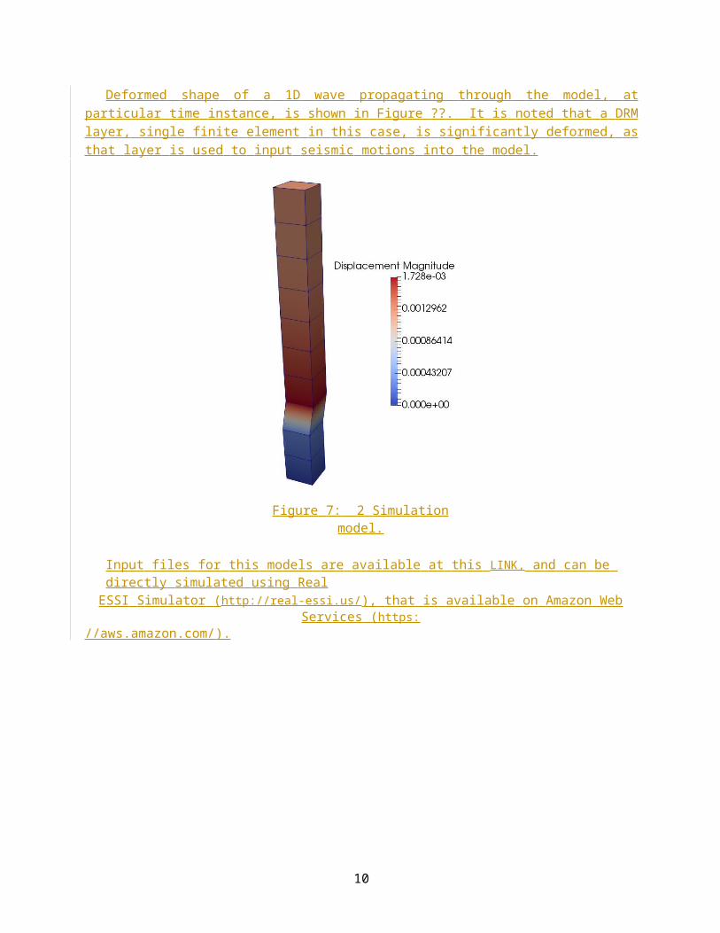
45m5m 10m

30m

65m 3x20

m5m

19

30m

2x15m

ContactDRM Layer

Damping Layers

Soil

100m 5m 10m

Figure 21: 6 Simulation Model.

Figure 22: 7 Simulation Model.

20

Acce

lera

tion

[m/s

^2]

Acce

lera

tion

[m/s

^2]

10 Time Series of Acceleration

2.5 FFT of Acceleration

Soil Surface Motion Structural Top Motion

Soil Surface MotionStructural Top Motion

2.05

1.5

0

1.0

50.5

10 0 1 2 3 4 5 6 7 8 9Time [s]

0.010-1

100

101

Frequency [Hz]

Figure 23: Simulation Results: Acceleration Time Series with 1D motion.

ReferencesBielak, J., Loukakis, K., Hisada, Y. & Yoshimura, C. (2003), ‘Domain reduction method for three–

dimensional earthquake modeling in localized regions. part I: Theory’, Bulletin of the Seismological Society of America 93(2), 817–824.

Idriss, I. M. & Sun, J. I. (1992), Excerpts from USER’S Manual for SHAKE91: A Computer Pro- gram for Conducting Equivalent Linear Seismic Response Analyses of Horizontally Layered Soil Deposits, Center for Geotechnical Modeling Department of Civil & Environmental Engineering University of California Davis, California.

Jeremi´c, B., Jie, G., Cheng, Z., Tafazzoli, N., Tasiopoulou, P., Abell, F. P. J. A., Watanabe, K., Feng, Y., Sinha, S. K., Behbehani, F., Yang, H. & Wang, H. (2018), The Real ESSI Simulator System, University of California, Davis and Lawrence Berkeley National Laboratory. http://real-essi.info/.

Kausel, E. (2006), Fundamental Solutions in Elastodynamics, A Compendium, Cambridge Uni- versity Press, The Edinburgh Building, Cambridge CB2 2RU, UK.

Kausel, E. (2017), Advanced Structural Dynamics, Cambridge University Press.

Kramer, S. L. (1996), Geotechnical Earthquake Engineering, Prentice Hall, Inc, Upper SaddleRiver, New Jersey.

Semblat, J.-F. & Pecker, A. (2009), Waves and Vibrations in Soils: Earthquakes, Traffic, Shocks, Construction works, first edn, IUSS Press.

Yoshimura, C., Bielak, J. & Hisada, Y. (2003), ‘Domain reduction method for three–dimensional earthquake modeling in localized regions. part II: Verification and examples’, Bulletin of the Seismological Society of America 93(2), 825–840.

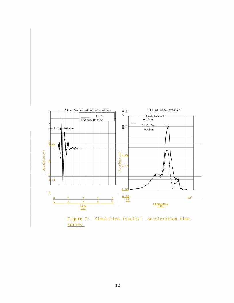
Pseu

do-S

pect

ral A

ccel

erati

on S

a [g

]Ps

eudo

-Spe

ctra

l Acc

eler

ation

Sa

[g]

Spec

tral

Dis

plac

emen

t [m

]Sp

ectr

al D

ispl

acem

ent [

m]

21

1.2 Pseudo-Spectral Acceleration 0.05 Spectral Displacement

1.0 0.04

0.8

0.03

0.6

0.4

0.02

0.20.01

0.010-1

100

101

102

Frequency [Hz]0.00 10-1

100

101

102

Frequency [Hz]

1.2 Pseudo-Spectral Acceleration 0.05 Spectral Displacement

1.0 0.04

0.8

0.03

0.6

0.4

0.02

0.20.01

0.0 0 1 2 3 4 5Period [s]

0.00 0 1 2 3 4 5Period [s]

Figure 24: Simulation Results: Response Spectrum of Structure Top with 1D motion.

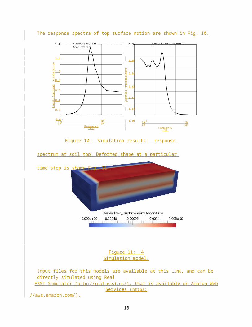
Acce

lera

tion

[m/s

^2]

Acce

lera

tion

[m/s

^2]

22

10 Time Series of Acceleration

Soil Surface MotionStructural Top Motion

2.5 FFT of Acceleration

Soil Surface MotionStructural Top Motion

2.05

1.5

0

1.0

50.5

10 0 1 2 3 4 5 6 7 8 9Time [s]

0.010-1

100

101

Frequency [Hz]

Figure 25: Simulation Results: Acceleration Time Series with 3D motion.

Pseu

do-S

pect

ral A

ccel

erati

on S

a [g

]

Spec

tral

Dis

plac

emen

t [m

]Sp

ectr

al D

ispl

acem

ent [

m]

23

1.2 Pseudo-Spectral Acceleration 0.05 Spectral Displacement

1.0 0.04

0.8

0.03

0.6

0.4

0.02

0.20.01

0.010-1

100

101

102

Frequency [Hz]0.00 10-1

100

101

102

Frequency [Hz]

1.2 Pseudo-Spectral Acceleration 0.05 Spectral Displacement

1.0 0.04

0.8

0.03

0.6

0.4

0.02

0.20.01

0.0 0 1 2 3 4 5Period [s]

0.00 0 1 2 3 4 5Period [s]

24

Figure 26: Simulation Results: Response Spectrum of Structure Top with 3D motion.

25

Structural response quantities

Deterministic analyses

8.7.1.1 Design forces, displacements and stressesThe structural response quantities (displacements, stresses, strains, bending moments, shear forces…) should be defined in accordance with the type of analysis used to compute them. Aside from the uncertainties in the soil and structural input data, which may be accounted for by sensitivity analyses, it must be realized that direct step by step analyses, as opposed to modal spectral analyses, introduce another cause of uncertainty in the response. This is due to the variability of the acceleration time histories derived from response spectra (see section 6.5). This variability is further enhanced when nonlinear step by step analyses are implemented. Some regulations (e.g. ASN Guide 2/01) recognize these possible sources of variability by specifying design quantities related to the type of analyses.

If Rk,i represents the maximum value of any response quantity for a given input motion, i (response spectrum or time history), and for one model (k) amongst the N models used for the sensitivity analyses, Rw,i is defined as a weighted average of these Rk,i:

88\* MERGEFORMAT ()

Note that the previous equation allows the designer to introduce any degree of conservatism in his design. The maximum value will be obtained, if model q gives the maximum response quantity, by setting wq = 1 and wp = 0 for all p ≠ q. An average value, over all sensitivity analyses, will be obtained by setting wk = 1/N for all k.

With this definition, it is suggested that the design structural response quantity, RD, be taken equal to:

For modal spectral analyses to

99\* MERGEFORMAT ()

For step by step linear time history analyses (with i=1, P time histories) to the mean value of the Rw,i , provided P ≥ 3;

1010\* MERGEFORMAT ()

For step by step nonlinear linear time history analyses (i=1, K) to the mean value plus some fraction of the standard deviation (Rw,i), provided K > 5; the fraction depends on the number K of simulations (time histories used for the analyses) and is based on the Student–Fisher test for a confidence interval of 95%. These values are provided in the following table.

K (K)5 0.95

26

6 0.827 0.738 0.679 0.62

10 0.5811 0.5512 0.5213 0.4914 0.4715 0.4520 0.3425 0.3430 0.3140 0.2750 0.24

In summary, any design quantity is given by

1111\* MERGEFORMAT ()

For modal spectral analyses, i=1, and for linear step by step analyses with i ≥3, (K)=0; for nonlinear step by step analyses with i ≥5, (K) is given in the previous table.

The rules detailed above are valid for design of new structures in deterministic analyses. For assessment of existing structures, Rw,i represents the value calculated for the best estimate properties (k=1, no sensitivity analyses) and the same rules apply.

8.7.1.2 Seismic input to sub-systemsThe seismic input to sub–systems is represented by the Floor Response Spectra (FRS). FRS are preferably calculated from the time histories of the response at the required location; however, methods used for direct generation of in-structure response spectra are acceptable when the system remains linear. They shall be computed in accordance with USNRC Regulatory Guide 1.122 and USNRC NUREG-800, 3.7.2, Rev. 3. Consideration should be given in the analysis to the effects on floor response spectra (e.g., peak, width) of expected variations of structural properties, damping values, soil properties, and SSI. In addition, for concrete structures, the effect of potential concrete cracking on the structural stiffness should be specifically addressed. To account for these uncertainties in the structural frequencies the computed floor response spectra from the floor time-history motions should be smoothed, and peaks associated with each of the structural frequencies should be broadened.

Amongst these parameters, the influence of the soil characteristics and time histories of the design earthquake are the most important. When multiple sets of time histories, derived from actual earthquake records, are used as the input motion to the supporting structure, the multiple sets of in-structure response spectra already account for some of the uncertainty (NUREG-800, 3.7.2) and there is no need to further broaden the peaks of the calculated FRS.

To account for the variability of the soil characteristics, at least three sets of velocity profiles should be used (section 8.6.2) for the analyses. In addition, the ASN2/01 guide recommends broadening by at least 15%, on either side, the peaks of the FRS associated with the best estimate soil properties.

27

Probabilistic analyses (Jim)o Internal forces, moments, displacement, stresseso Seismic input to sub-systems

Appendices: Examples Site response analyses:

o Develop approaches 1,2, 3 SSI analysesIncoherence

REFERENCES

Assimaki, D., Pecker, A., Popescu, R., Prevost, J.H., Effects of spatial variability of soil properties on ground surface motion, Journal of Earthquake Engineering, 7(1):1–44, 2003.

De Barros, F.C., Luco, E., Discrete models for vertical vibrations of surface and embedded foundations, Earthquake Engineering and Structural Dynamics, 19: 289–303, 1990.

Kolias, B., Fardis, M.N., Pecker, A., Designers' Guide to Eurocode 8: Design of Bridges for Earthquake Resistance, CRC Press, Taylor and Francis group, London, 258 pages, 2012.

Pecker, A., Enhanced seismic design of shallow foundations: example of the Rion Antirion Bridge, 4 th

Athenian Lecture on Geotechnical Engineering, 2006.

Popescu, R., Stochastic variability of soil properties: Data analysis, digital simulation, effects on system behaviour, PhD thesis, Princeton University, Princeton, New Jersey, 1995.

Popescu, R., Prevost, J. H., Deodatis, G., Effects of spatial variability on soil liquefaction: Some design recommendations, Geotechnique 47(5): 1019-1036, 1997.

Saitoh, M., On the performance of lumped parameter models with gyro mass elements for the‐ impedance function of a pile group supporting a single degree of freedom system, Earthquake‐ ‐ ‐ ‐ Engineering and Structural Dynamics, 41: 623–641, 2012.

Wolf, J.P., Foundation vibration analysis using simple physical models. Prentice Hall Inc, 1994.