University Duisburg – Essen

Department of Chemistry

Curriculum “Water: Chemistry, Analysis, Microbiology”

Characterisation and efficiency test of a decentralized water purification

system (pilot phase)

Bachelor Thesis

for attainment of the academic degree of

Bachelor of Science

presented by

Timo Jentzsch

Westmarkstraße 80

46149 Oberhausen

Period of work: from 11th

April 2005 to 11th

August 2005

Supervisor: PD Dr. Heinz-Martin Kuß

Analytical Chemistry

Declaration:

Herewith I declare that this thesis is the result of my independent work. All sources

and auxiliary materials used by me in this thesis are cited completely.

Duisburg, . . . . . . . . (Signature)

2

Host Supervisor: Mr. Eugene Sihle Ngcobo

Institution: Walter Sisulu University (formerly Border Technikon),

East London, South Africa

Department: Analytical Chemistry

3

I. Abstract

South Africa is a country, which is currently categorised as water stressed. The

International Water Management Institute (IWMI) has predicted a scenario of water

scarcity by the year 2025. Studies have been done to find a way to avoid this future

scenario. They have led to the conclusion that a sustainable water management is

necessary. These management tools include strategies of wastewater management,

among others. One example is the treatment and reuse of wastewater directly on-

site, especially in rural areas and urban settlements, which are not connected to the

municipal sewage system.

This can be done with decentralized water purification systems.

A system of this type has been installed at the Lilyfontein School in the Eastern Cape

province of South Africa.

It is based on the principle of a submerged fixed-film bioreactor. This system consists

of four parts: a balancing tank, the two bioreactors and a clarifier. The wastewater is

pumped from the balancing tank, which serves as a second septic tank, into the first

bioreactor. This tank is packed with a plastic material with a big surface. The sludge

in the water can settle down on this material to form biofilms with many different

types of bacteria. Because of external aeration oxidation reactions take place, which

are carried out by these microorganisms. The same happens in the second

bioreactor. Finally the water ends up in the clarifier, where it is disinfected and stored

until it is pumped into a big reservoir.

In this project samples were taken from the four parts of the system over a period of

approximately two months to characterise this biological wastewater treatment plant

and to test its efficiency. The parameters examined were the physical-chemical

parameters temperature, pH, electrical conductivity (EC), dissolved oxygen (DO) and

the chemical oxygen demand (COD), as well as ammonia-nitrogen and the anions

fluoride, chloride, nitrite, bromide, nitrate, phosphate and sulphate.

The results for the effluent were compared to the Target Water Quality Range

(TWQR) provided in the South African Water Quality Guidelines, Volume 4:

Agricultural Use: Irrigation. These guidelines were used because the final effluent is

intended to be used for irrigation. This paper only covers the first phase of a bigger

project. The major aim is to get a base of knowledge about this kind of wastewater

treatment to convince municipalities and governments to install such systems in rural

areas and urban settlements, which are not connected to the municipal sewage

system.

The water purification system showed to have a COD removal rate of 73% and a

nitrification, which causes an ammonia removal rate of 95%. This is an indication that

the system is working properly and the water is purified successfully. The only

restriction is the lack of a denitrification so that the nitrate levels in the effluent are too

high. A possible solution to solve this problem is suggested in this paper.

4

II. List of abbreviations

cm centimetre

COD chemical oxygen demand

DO dissolved oxygen

DWAF Department of Water Affairs and Forestry

EC electrical conductivity

EPS extracellular polymeric substances

FAO Food and Agriculture Organisation of the United Nations

IC ion chromatography

IWMI International Water Management Institute

KHP potassium hydrogen phthalate

km2

square kilometres

l litre

m metre

m3

cubic metre

mg milligram

ml millilitre

mm millimetre

mS milliSiemens

n. d. not detectable

nm nanometre

PE polyethylene

UV ultraviolet (spectrum of light)

VIS visible (spectrum of light)

WSU Walter Sisulu University

WTW Wissenschaftlich Technische Werkstätten

µS microSiemens

5

Table of contents

I. Abstract…………………………………………………………………………...3

II. List of abbreviations……………………………………………………………..4

1. Introduction………………………………………………………………………………6

1.1 South Africa and its water problems…………………………………………..6

1.2 The submerged fixed-film bioreactor………………………………………….7

1.3 Guidelines and parameters……………………………………………………10

1.3.1 Physical-chemical parameters……………………………………...11

1.3.2 Anions…………………………………………………………………12

2. Aims………………………………………………………………………………………15

3. Material and methods…………………………………………………………………16

3.1 Deionised water………………………………………………………………..16

3.2 Cleaning of equipment………………………………………………………...16

3.3 Taking the samples…………………………………………………………….16

3.4 On-site measurements………………………………………………………...17

3.4.1 pH and temperature…………………………………………………17

3.4.2 Electrical conductivity……………………………………………….18

3.4.3 Dissolved oxygen……………………………………………………19

3.5 Spectrophotometer…………………………………………………………….20

3.6 Chemical oxygen demand…………………………………………………….20

3.7 Anions…………………………………………………………………………...22

3.8 Ammonia-nitrogen……………………………………………………………..26

4. Results…………………………………………………………………………………...28

4.1 Appearance and smell…………………………………………………………28

4.2 Physical-chemical parameters………………………………………………..28

4.2.1 Temperature………………………………………………………….29

4.2.2 pH……………………………………………………………………...31

4.2.3 Electrical conductivity………………………………………………..32

4.2.4 Dissolved oxygen…………………………………………………….33

4.2.5 Chemical oxygen demand…………………………………………..35

4.3 Anions and ammonia…………………………………………………………36

4.3.1 Fluoride………………………………………………………………36

4.3.2 Chloride………………………………………………………………37

4.3.3 Bromide………………………………………………………………39

4.3.4 Phosphate……………………………………………………………39

4.3.5 Sulphate……………………………………………………………...40

4.3.6 Nitrogen………………………………………………………………41

5. Discussion……………………………………………………………………………...43

6. References……………………………………………………………………………...46

7. Appendix………………………………………………………………………………..48

6

1. Introduction

1.1 South Africa and its water problems

The Republic of South Africa is the southernmost country on the African continent. Its

area of 1.22 million km2

is bordered by Botswana and Zimbabwe to the north,

Mozambique and Swaziland to the northeast and east, the Indian Ocean to the

southeast and south, the Atlantic Ocean to the southwest and west, and Namibia to

the northwest. In the eastern part of the country the independent constitutional

monarchy of Lesotho is surrounded by South African territory. The population of

South Africa is approximately 45.4 million, estimated in 2004. 42 % of it is considered

as rural. The average population density is 37 inhabitants/km2

. It ranges from 21 in

rural to more than 100 inhabitants/km2

in urbanised areas.

South Africa is a net food exporter. Nevertheless one third of the population is

strongly vulnerable to food shortages because of poverty and the lack of suitable

infrastructure in the deep rural areas. This problem could be solved by homegrown

vegetables (FAO, 2005).

But most parts of the country are considered as arid or semi-arid land, which means

that 65 % of South Africa is receiving too less rainfall for agriculture.

An annual rainfall of at least 500 mm/year is required for successful dry land farming.

But South Africa’s average rainfall is only 450 mm/year (the world average is 860

mm/year). That leads to the conclusion that irrigation is necessary for agriculture.

Therefore it is no surprise that 60 % of the total water requirements of South Africa

are represented by agriculture. Because of that high water demand and the low

annual rainfall the water resources of the country are scarced and limited (Otieno and

Ochieng, 2004).

This has dramatic consequences on the population because of a decrease of the

annual freshwater availability. According to Otieno and Ochieng (2004) the annual

freshwater availability in South Africa is estimated by the FAO to 1154 m3

per

capita/year. While the index for water stress is 1700 m3

per capita/year, the country is

categorised as water stressed (Otieno and Ochieng, 2004).

The annual population growth rate is estimated at about 1.2 % (FAO, 2005). Based

on that the water demand projections in South Africa indicate an annual growth rate

of 1.5 % between 1990 and 2010 (Otieno and Ochieng, 2004). That leads to further

problems in the future. Otieno and Ochieng presented a report in 2004 suggesting

water management tools to avert these problems. They refer to an estimation of the

International Water Management Institute (IWMI) that by the year 2025 South Africa

will face a scenario of physical water scarcity because the annual freshwater

availability will be less than 1000 m3

per capita, which is the index for water scarcity.

These water management tools suggest possible solutions to avert this future

scenario. Some of them are the demand management of water, identifying and

developing alternative supply systems, applying techniques to improve water quality

for particular uses and the water transfer from surplus areas to deficit areas (Otieno

and Ochieng, 2004).

Another reason for the decreasing availability of clean drinking water is the pollution

of surface waters and groundwater by the discharge of wastewater. This is especially

a problem in developing countries like South Africa. On the one hand the polluted

water bodies require expensive treatment techniques to clean the water to drinking

water standards. And on the other hand the water is just not used efficiently so that it

is simply wasted. That leads to the conclusion that sustainable wastewater

management strategies have to be developed.

7

Nhapi and Gijzen (2005) describe a “3-step strategic approach to sustainable

wastewater management”. The first step is the minimisation of wastewater

generation. This can be achieved by the reduction of water consumption and waste

generation. For example only two litres of the drinking water consumed in an average

household per person and day are really used for drinking and cooking. The rest (150

– 350 litres per person and day) is used for other purposes like washing, hygiene,

gardening and flushing of toilets where water of drinking quality is not necessary. It

can be suggested that water of different qualities should be delivered for different

uses. This leads to the second step. This step describes the treatment and reuse of

wastewater. In a third step it is suggested that after successful employment of the

first two steps the remaining wastewater can be carefully discharged into receiving

water bodies so that the self-purification capacity of these waters is stimulated (Nhapi

and Gijzen, 2005). The problem with the second step is that facilities for the

treatment of wastewater are very expensive. In most countries, centralized

wastewater treatment plants are treating the wastewater of bigger settlements like

cities. But in developing countries like South Africa many rural areas with a very low

population density exist. Therefore centralized wastewater treatment is nearly

impossible because it would be highly uneconomic. The solution lies in decentralized

wastewater treatment systems. These systems treat the wastewater on-site in single

households or other building clusters which are not connected to the municipal

sewage system. The purified water can then be used for irrigation or other purposes

where no water of drinking quality standard is necessary, or it can be discharged into

the environment. Different systems are described in the literature, most of them

working with biological methods for the removal of nutrients from domestic

wastewater. These are, for example, constructed wetlands (Verhoeven and

Meuleman, 1999), anaerobic baffled reactors (Foxon et al., 2004) and membrane

bioreactors, also called fixed-film bioreactors (Oh et al., 2001; Ho et al., 2001;

Lesjean et al., 2002; Cicek, 2003).

This project is focussing on the characterisation and efficiency testing of such a

decentralized water purification system based on the principle of a submerged fixed-

film bioreactor.

1.2 The submerged fixed-film bioreactor

A submerged fixed-film bioreactor is a system, which can purify wastewater on

biological basis without the addition of chemicals, which are expensive and

sometimes hazardous to the environment. A certain medium with a large specific

surface is submerged in a tank, which is filled with wastewater. In most cases it is a

plastic material. The sludge and other suspended matter in this water contain many

different microorganisms. These microorganisms develop on their own. They settle

down on the medium to form so-called biofilms. A biofilm is the agglomeration of

many microorganisms on a surface. It is made of extracellular polymeric substances

(EPS), which are created by these microorganisms. It can be seen as the “house” of

the bacteria. They are living there and are protected against external influences, for

example chemicals or antibiotics (Madigan et al., 2003).

Once these biofilms have built up properly on the surface of the material in the

biofilter, the wastewater flowing over this surface is purified because the bacteria gain

the energy necessary for their metabolism by oxidising the energy-rich organic

compounds in the wastewater (Rüffer and Masannek, 2002). The dissolved oxygen in

the wastewater is almost completely consumed for these reactions. That means that

additional oxygen is needed to create aerobic conditions. This is achieved by

8

external aeration. In most cases normal air from the surroundings is pumped into the

water by using an electrical pump.

A decentralized water purification system of this type was installed at the Lilyfontein

School in the Eastern Cape province of South Africa. This system was the object of

interest for this project. This school is located in a rural area and not connected to the

sewage system of the Buffalo City Municipality.

Lilyfontein School

Figure 1: map of the Eastern Cape province (modified)

Most of the wastewater in this school comes from the toilets, which are used by

approximately 300 persons (pupils and teachers), according to the caretaker of the

school.

The raw sewage is flowing into a septic tank which is installed underground. Here it is

stored on the one hand and on the other hand some reactions can take place in

these anaerobic to anoxic conditions. These reactions are carried out by

microorganisms (e.g. bacteria) and include mostly the biodegradation of the organic

compounds in the sewage. The most important products of these reactions are water

(H2O) and carbon dioxide (CO2), but also the toxic gases hydrogen sulphide (H2S)

and ammonia (NH3), which give the wastewater an offensive odour. Heavier solids

settle down on the ground of the tank while lighter ones are floating on the water

surface, forming a scum layer. The cleaner water in the middle can flow out of the

tank. But up to 70% of the pollutants are still in this water, so that further treatment is

essential (Johnston and Smith, 2005). For this reason the system mentioned above

was installed at Lilyfontein School by the company “Clearedge”. This system can

purify septic tank effluent with biological methods. No hazardous chemicals and very

low maintenance are needed (Clearedge, 2005).

9

Bioreactor 1 Bioreactor 2

Clarifier

Balancing tank

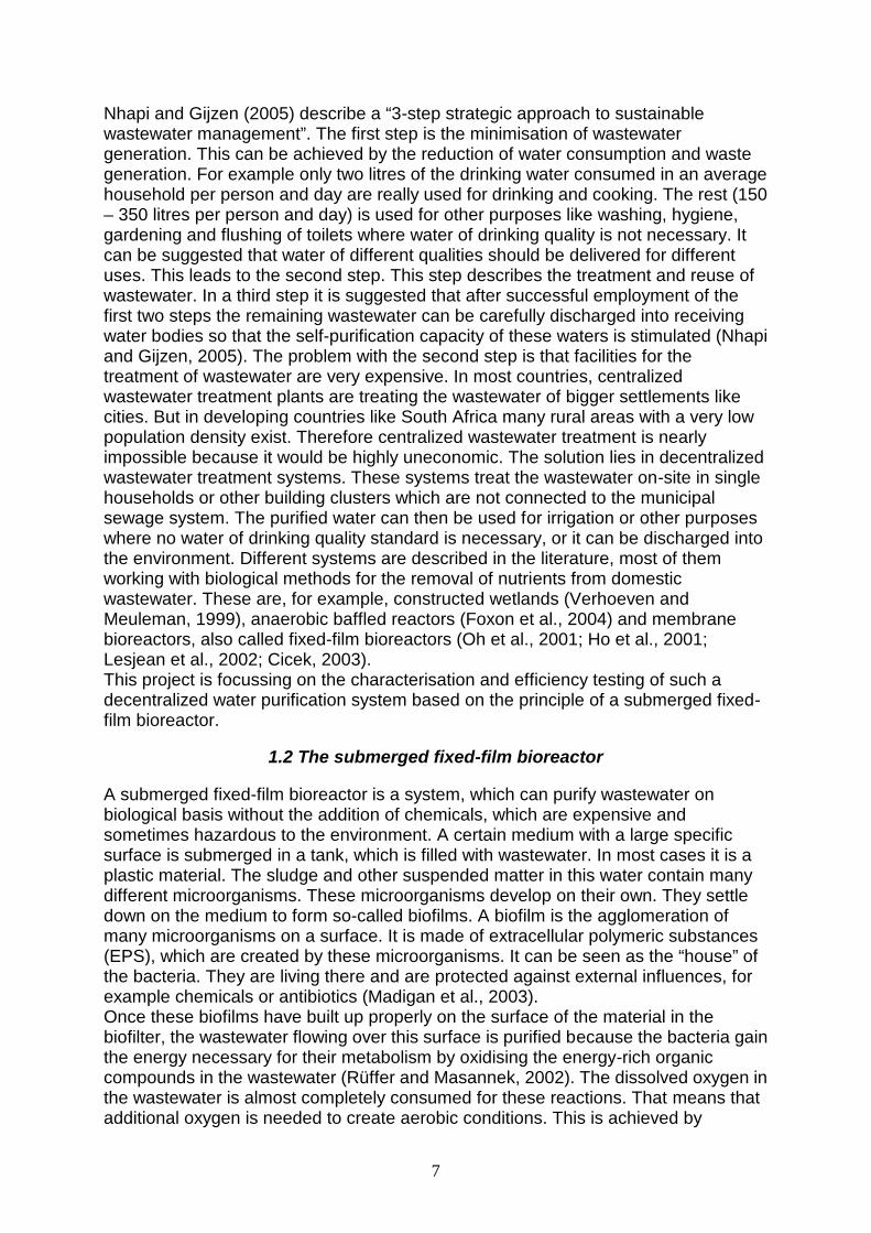
Figure 2: wastewater treatment system at Lilyfontein School

The photography above (Figure 2) shows the complete wastewater treatment system

installed at Lilyfontein School. The effluent from the septic tank first flows into the

balancing tank. This tank serves as a second septic tank where the same processes

take place as in the original septic tank. It is also installed to store some of the

wastewater so that the bioreactors are not overloaded by too much water. From this

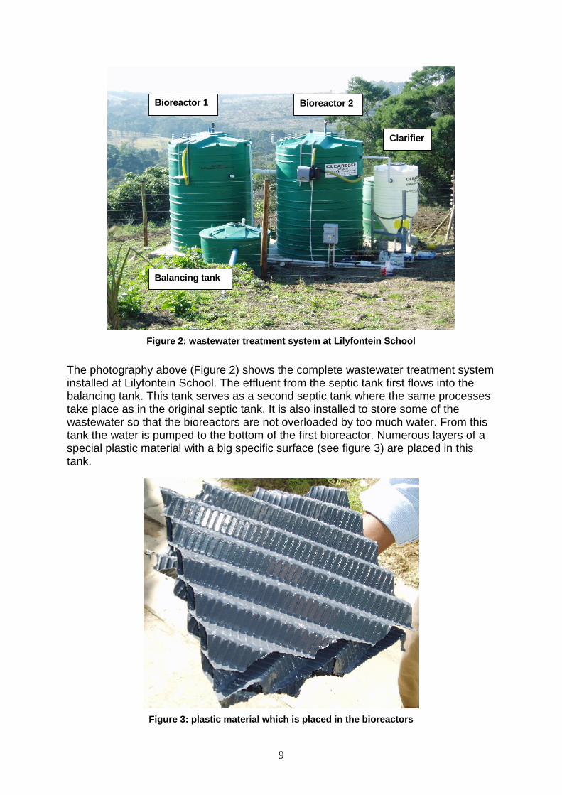
tank the water is pumped to the bottom of the first bioreactor. Numerous layers of a

special plastic material with a big specific surface (see figure 3) are placed in this

tank.

Figure 3: plastic material which is placed in the bioreactors

10

The sludge in the wastewater, which contains many different microorganisms, can

settle down on this surface to form biofilms, as explained above. As the water level

rises, the wastewater has contact to these biofilms, which act like a biofilter. The

bacteria feed on the nutrients and decompose the organic compounds in the water.

For these reactions high amounts of oxygen are needed. To create these aerobic

conditions, a pump is installed on the outside wall of the tank to pump air from the

surroundings into the water. When the tank is filled to the top, the water can flow

through a connection pipe into the second bioreactor. It is exactly the same as the

first one, with the only exception that the water enters from the top and not from the

bottom. External aeration is also used. The retention time of the water is 24 hours for

each bioreactor. After that the treated water flows into the clarifier. Here the

remaining solids and bacteria which might have been washed off from the biofilms

can settle down to form a sludge layer at the bottom of this tank. It has a conical

shape so that it can be desludged by opening a valve at the bottom. The sludge flows

back into the balancing tank so that the bacteria in it can be reused in the purifying

process. Desludging is only necessary once in a month because there is not very

much sludge in the purified water. Also once in a month a chlorine tablet, which is

commercially available for the chlorination of swimming pools, is added to the water

in the clarifier to kill remaining pathogenic microorganisms in the purified water. This

is the only chemical needed in this system. But it is not essential. It depends on the

amount of pathogens in the water. Some of these treatment plants can also run

without disinfections, according to the manufacturer. This water, also called final

effluent, is pumped into a big reservoir from where it can be taken for the different

reuse activities, in this case irrigation of the rugby field or toilet flushing. But before

the water can be reused, the quality of the final effluent has to be monitored to check

if it fits the guidelines and limits set by the government.

1.3 Guidelines and parameters

There are no guidelines available for the quality of water used for toilet flushing. The

only limiting factors might be aesthetic aspects like colour and smell.

For that reason only the guidelines for irrigation are considered in this project.

The custodian for South Africa’s water resources is the Department of Water Affairs

and Forestry (DWAF). This department has the mission to ensure that the quality of

water resources remains fit for specific use sectors and to maintain and protect

aquatic ecosystems. Therefore the South African Water Quality Guidelines have

been developed. They serve as a source of information to achieve these goals

(DWAF, 1996). Guidelines are available for several different use sectors. Because

the final effluent is aimed to be used for irrigation, only the following guideline is

considered for this project:

Volume 4: Agricultural Use: Irrigation

Many different parameters have to be monitored to check if their values are within the

Target Water Quality Range (TWQR). It is defined as “the range of concentrations or

levels at which the presence of a particular constituent would have no known or

anticipated adverse effects on the fitness of water for a particular use” (DWAF, 1996).

It has to be mentioned that this definition includes the information that water, which

does not fit in the TWQR, can still be used for the desired purpose under certain

circumstances.

The parameters monitored in this project have been chosen according to their

importance and the availability of equipment to determine them.

11

1.3.1 Physical-chemical parameters

The temperature of water can be expressed in different units. In this project it is

expressed as degrees on the Celsius temperature scale (°C). The temperature has

no direct effect on the water quality. But it can influence the biological activity and the

solubility of oxygen in water. The higher the temperature, the lower the concentration

of dissolved oxygen. On the other hand processes and reactions taking place in the

water can affect the temperature. The South African Water Quality Guidelines

provide no TWQR for the temperature (DWAF, 1996)

The pH is defined as the negative logarithm to the base ten of the hydrogen ion

activity. The pH scale ranges from 0 to 14. A pH of 7 means that the solution is

neutral. If it is lower, the solution is acidic, and if it is higher, the solution is basic.

Except at extremes, the pH value of water has no direct effects on the water quality.

But it can cause adverse effects by solubilisation of toxic heavy metals and the

protonation and deprotonation of other ions. And extreme pH values can induce

corrosion of the irrigation equipment. The TWQR for irrigation is 6.5 to 8.4 (DWAF,

1996).

The electrical conductivity (EC) describes the amount of ions in water. These ions

carry an electrical charge and therefore the water can conduct an electrical current,

which is measured electrochemically. The unit of the EC is milliSiemens per meter

(mS/m). The conductivity is dependent on the value of the electrical charge of the

different ions, to mobility of these ions and their concentration. Water with a high EC

is also called saline water. By using this for irrigation, salt is induced into the soil

profile where it accumulates. This creates a saline soil. While many commercial crops

are sensitive to soil salinity, they cannot be grown successfully because the crop

yield is reduced. The TWQR for the EC of water for irrigation is < 40 mS/m, where

most of the crops and other plants can grow. The higher the EC, the lower the crop

yield and the choice of crops that can be grown successfully (DWAF, 1996).

The dissolved oxygen (DO) is the amount of gaseous oxygen dissolved in water. It

is given in milligrams per litre (mg/l). The concentration of the dissolved oxygen

depends on the biological and chemical processes and reactions, which can take

place in the water where oxygen is either consumed or released. But it also depends

on the temperature. The higher the temperature, the lower the solubility of oxygen,

which results in a lower concentration. Water with 100% saturation of oxygen has a

concentration of 9.1 mg/l at 20 °C (Grohmann and Nissing, 2002). Wastewater

normally has a very low DO concentration because of the high chemical oxygen

demand. A TWQR is not available.

The chemical oxygen demand (COD) is a measure for the sum of all organic

compounds in a water sample, including the heavily degradable ones. The COD

value signs the amount of oxygen used for the oxidation of the entire organic

compounds in the water sample. It is given in mg O2/l. The COD is an important

parameter for the characterisation of the efficiency of a wastewater treatment plant.

A high COD indicates a high organic load in the water, which is typical for

wastewater. The dissolved oxygen in the water is consumed so that its concentration

is very low. (Standard Methods, 1998; Rüffer and Masannek, 2002). The South

African Water Quality Guidelines for irrigation do not provide a TWQR for the COD.

12

1.3.2 Anions

Fluoride is the anion of fluorine, which is the most electronegative member of the

halogens and therefore the most reactive one. Fluorides occur in natural waters

because of the leaching from fluoride containing minerals into the groundwater

source. If the fluoride concentration is not excessively high, the irrigation with this

water does not have adverse effects on the crop yield because most crops are

relatively tolerant towards fluoride. And while fluoride normally does not accumulate

in the crops, there are no health risks for animal or human consumption.

Nevertheless the TWQR is set to < 2.0 mg/l (DWAF, 1996).

Chloride is the anion of chlorine. It is an essential micronutrient for plants and

relatively non-toxic to them. Chlorides are highly soluble and do not tend to be

absorbed by the soil in a significant degree. Therefore they are taken up by the plant

roots and/or leaves, depending on the irrigation method. High chloride concentrations

can cause plant injuries, which result in a decrease of crop yield. When chloride

accumulates in the leaves, foliar damage like leaf burn can occur, which is especially

a problem when the leaves are the marketed product. Because of the high solubility,

chlorides can only be removed by expensive processes, for example reverse

osmosis. Using such a technique for the treatment of water designated for irrigation

would be highly uneconomic. The farmer should either accept the decreased crop

yield or switch to plants, which are more tolerant towards chloride.

The chloride concentrations in fresh water can vary from a few to several hundred

mg/l; in seawater it is approximately 19800 mg/l. The TWQR is 100 mg/l. This is the

threshold where no adverse effects occur in most plants (DWAF, 1996).

Bromide is the anion of the element bromine. No adverse or anticipated effects are

known for irrigation with water containing bromide. Therefore no TWQR is available

in the South African Water Quality Guidelines (DWAF, 1996).

Sulphate is a common constituent of many waters. It occurs in natural waters

because of the leaching of sulphate minerals from the sediment into the water body

(Grohmann et al., 2002). While it is not essential for the human body, the sulphate

taken up with drinking water is excreted via the urine and faeces. Therefore

sulphates also occur in wastewater. Under anaerobic or anoxic conditions they are

reduced to sulphides and form the toxic gas hydrogen sulphide, which gives the

wastewater an offensive odour. The bacteria responsible for these reduction

processes are of the species Desulfovibrio and Desulfobacter (Brock, 2003). But the

sulphides in the wastewater also come from the decomposition of organic

compounds like proteins.

In biological wastewater treatment under aerobic conditions the bacteria Thiobacillus

thiooxidans oxidise the sulphides to sulphate again.

While no adverse or anticipated effects are known for the irrigation with sulphate

containing water, no TWQR is given by the South African Water Quality Guidelines.

Phosphate, in this case ortho-phosphate (PO4

3-

), is one of the phosphorous species

occurring in wastewater. As an essential part of the human body, 1% of the body

mass is phosphorous and is taken up in the form of phosphates. The organism can

handle variations in the uptake of phosphorous compounds by mobilisation of parts

of this big phosphorous stock. Therefore most phosphates in wastewater come from

13

human excrements (Grohmann et al., 2002). Phosphorous is playing an important

role in the biological wastewater treatment because it is also an essential nutrient for

the microorganisms. They can take up phosphorous in almost every form.

This is the same case for plants. Therefore many farmers buy fertilisers containing

phosphorous. Therefore the South African Water Quality Guidelines do not provide a

TWQR for phosphate in irrigation water (DWAF, 1996).

The only problem, which can occur, is eutrophication. Eutrophication describes the

scenario when high loads of nutrients (mostly nitrogen and phosphorous) enter the

surface water bodies. These nutrients promote excessive growth of algae and

cyanobacteria, which create high amounts of organic matter when they die, as well

as toxins, which are hazardous for fish and other water animals. The bacteria which

decompose these organic loads consume very much of the dissolved oxygen so that

the conditions switch from aerobic over anoxic to anaerobic. That leads to the death

of other water organisms dependent on the oxygen dissolved in the water, mostly

fish. The result of all that is the beginning of fouling processes of the water creating

methane, carbon dioxide and hydrogen sulphide, so that these processes can be

seen as that death of the water (Rüffer and Masannek, 2002; Brock, 2003).

Nitrogen can occur in various forms. On the one hand there are organic nitrogen

compounds and on the other hand there are the inorganic compounds ammonia,

nitrite and nitrate. The interconversion and co-existence of these different forms of

nitrogen are known as the nitrogen cycle, which can be used to describe the

processes in biological wastewater treatment. The organic compounds, for example

amino acids, are decomposed by bacteria with ammonia as one of its products.

Under aerobic conditions the organic nitrogen compounds can also be oxidised to

nitrate. Ammonia is a toxic gas, which gives the wastewater, together with hydrogen

sulphide, methane and other gases, a bad smell. It can be eliminated by a process

called nitrification. This process requires aerobic conditions. In a first step ammonia is

oxidised to nitrite. This is done by bacteria of the species Nitrosomonas. In a second

step bacteria of the species Nitrobacter oxidise the nitrite to nitrate, which is the end

product of the nitrification. Nitrate is, like phosphorous, a key nutrient for plants. It is

also contained in fertilisers. But if the concentration is too high, it can also cause

eutrophication problems, as explained above. For the nitrate removal further

treatment is required. Bacteria of the species Bacillus, Paracoccus and

Pseudomonas carry out a process called denitrification. Under anoxic conditions

these bacteria use the oxygen contained in the nitrate for their respiration by

reducing the nitrate to gaseous elemental nitrogen, which is released to the

atmosphere (DWAF, 1996; Rüffer and Masannek, 2002; Brock, 2003).

The South African Water Quality Guidelines provide a TWQR of 5 mg/l for the sum of

all inorganic nitrogen species. Ammonia, nitrite and nitrate are considered together

because of their interconversion and co-existence in aquatic systems. Although

nitrogen is an essential nutrient for plants, the TWQR is set relatively low because

too high concentrations of nutrients can have detrimental effects on most plants and

nitrate not taken up by the plants can contaminate the groundwater. Another reason

is that a nutrient overload of the irrigation water can promote algal growth inside the

irrigation equipment, which leads to clogging of it (DWAF, 1996).

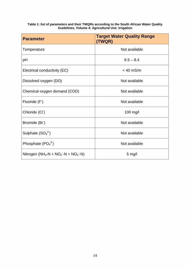
A summary of the parameters and their TWQRs can be viewed in table 1.

14

Table 1: list of parameters and their TWQRs according to the South African Water Quality

Guidelines, Volume 4: Agricultural Use: Irrigation

ParameterTarget Water Quality Range

(TWQR)

Temperature Not available

pH 6.5 – 8.4

Electrical conductivity (EC) < 40 mS/m

Dissolved oxygen (DO) Not available

Chemical oxygen demand (COD) Not available

Fluoride (F-

) Not available

Chloride (Cl-

) 100 mg/l

Bromide (Br-

) Not available

Sulphate (SO4

2-

) Not available

Phosphate (PO4

3-

) Not available

Nitrogen (NH3-N + NO2

-

-N + NO3

-

-N) 5 mg/l

15

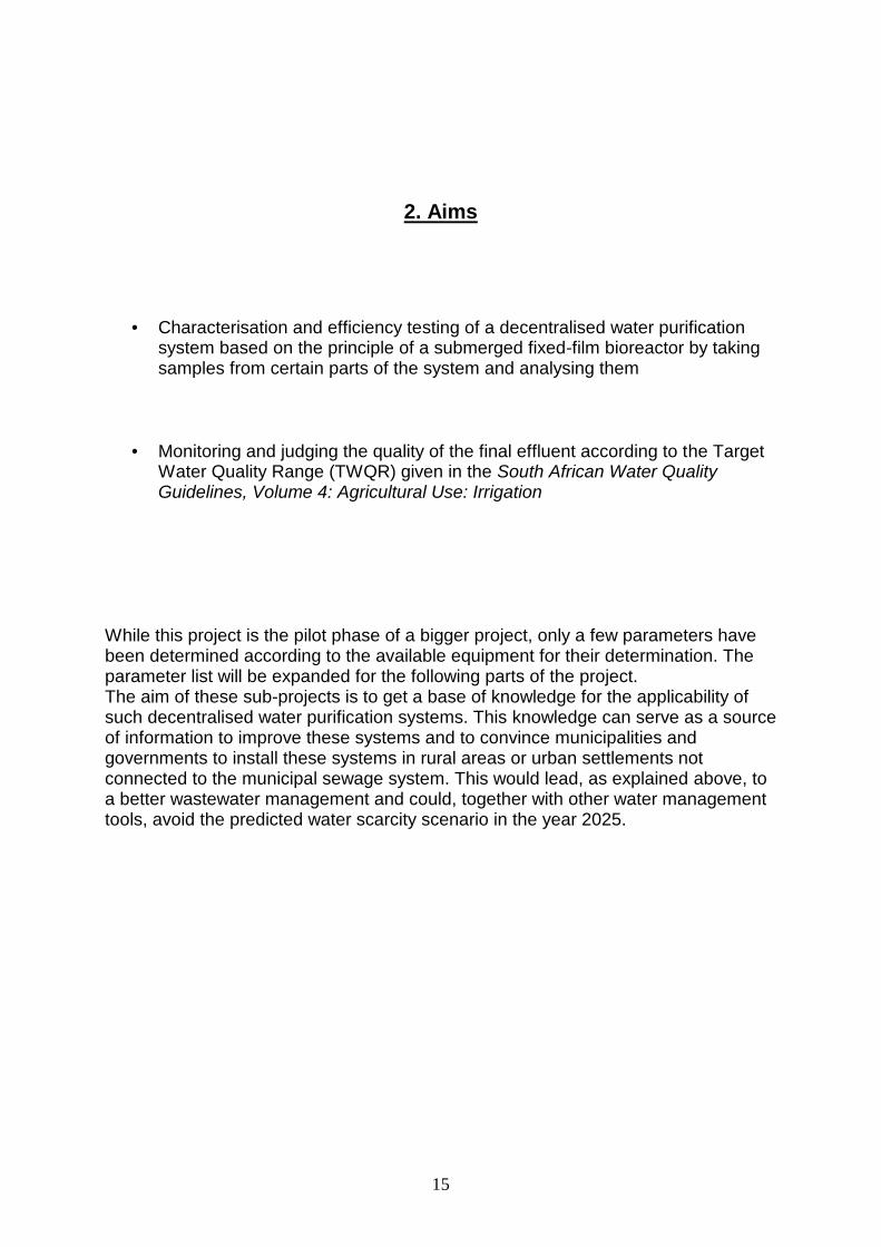
2. Aims

• Characterisation and efficiency testing of a decentralised water purification

system based on the principle of a submerged fixed-film bioreactor by taking

samples from certain parts of the system and analysing them

• Monitoring and judging the quality of the final effluent according to the Target

Water Quality Range (TWQR) given in the South African Water Quality

Guidelines, Volume 4: Agricultural Use: Irrigation

While this project is the pilot phase of a bigger project, only a few parameters have

been determined according to the available equipment for their determination. The

parameter list will be expanded for the following parts of the project.

The aim of these sub-projects is to get a base of knowledge for the applicability of

such decentralised water purification systems. This knowledge can serve as a source

of information to improve these systems and to convince municipalities and

governments to install these systems in rural areas or urban settlements not

connected to the municipal sewage system. This would lead, as explained above, to

a better wastewater management and could, together with other water management

tools, avoid the predicted water scarcity scenario in the year 2025.

16

3. Material and Methods

3.1 Deionised water

The water used for rinsing the equipment (sampling bottles, glassware, pipette tips,

syringes) and preparing of solutions was taken from the MilliQ-System (MilliPore) in

the chemistry lab at WSU.

The tap water is first filtered through a filter with a pore diameter of 1 µm. Then it is

treated with activated charcoal. After that it runs through a second filter with 0,5 µm

pores. This is followed by the Milli-RO-System. Here the water is first run over an ion

exchange resin and then pushed through a reverse osmosis membrane to hold back

most of the ions present in the water. This treated water is stored in a reservoir tank.

When water is needed, it is pumped from this tank through the Milli-Q-System, which

also consists of an ion exchange resin to purify the water to a very pure grade.

3.2 Cleaning of equipment

The equipment used in this project (glassware, sampling bottles, pipette tips,

syringes) had to be kept clean to avoid contaminations, which could falsify the results

of the experiments. First the equipment was soaked in water containing a detergent.

After that it was rinsed with tap water until it was free of detergent. Finally it was

rinsed at least three times with deionised water.

3.3 Taking the samples

Samples were taken in the period from May 11th

to July 8th

.

The PE-bottles used for taking the samples were delivered by Amatola Water, a local

water supplier. They were cleaned as explained above. Samples were taken two to

three times a week. The sampling sites are indicated in figure 1. Samples were taken

from the clarifier (sample “Eff”) to determine the quality of the final effluent, as well as

from the balancing tank (sample “In”) to determine the efficiency of the treatment

plant. From the third week on (27.05.05) samples were also taken from the two

bioreactors (samples “Bio1” and “Bio2”) to get a better understanding of the

processes taking place in them.

The sampling procedure was the same for each sample. First the screw cap on the

respective tank was opened. Then the sample bottle was submerged into the water

to fill it. The bottle was rinsed twice with this water before filling it to the top.

After that the bottle was closed and stored in a cooler box. This was necessary to

avoid alterations of the samples between the sampling and the analyses because the

Lilyfontein School is approximately 50 km away from the laboratory.

Prior to the determinations done in the laboratory the samples were allowed to reach

room temperature.

At July 7th

one sample was also taken from the school’s borehole to roughly estimate

the quality of the groundwater there. This groundwater is mainly used there for

flushing the toilets. This was done to help in the explanation of some of the other

results.

17

3.4 On-site measurements

3.4.1 pH and temperature

Principle:

Today the most common method for the determination of the pH value of a water

sample is the potentiometric method using a glass electrode. This glass electrode

consists of a glass body filled with a buffer solution with a known pH and an inner

reference electrode, in most cases a silver/silver chloride electrode. The layer of the

glass electrode can be described as a glass membrane with the exception that the

hydrogen ions cannot go through the membrane completely. This glass layer serves

as a buffer of silicic acid and silicate where cations can be exchanged. This leads to

a development of differences in the potential between the membrane and the

evaluated solution on the one side, and differences in the potential between the

membrane and the buffer solution on the other side of the membrane. These

differences in the potential are evaluated to determine the pH. While the pH of the

internal buffer solution is known, the unknown pH can be calculated by subtraction of

the potential of the known solution from that of the unknown solution. But to make an

absolute evaluation possible, the pH electrode has to be calibrated with a

standardised buffer with a known pH. Immersing the electrode in the buffer gives the

potential difference EB and immersing in the unknown solution gives the potential

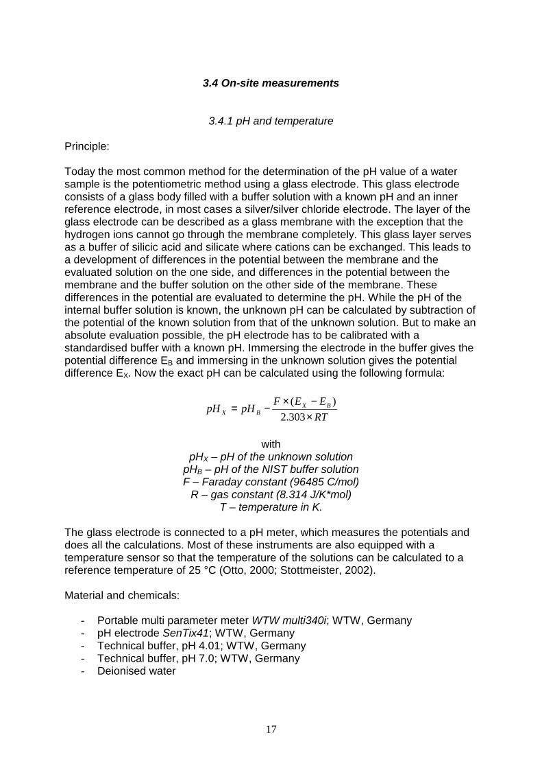
difference EX. Now the exact pH can be calculated using the following formula:

RT

EEF

pHpHBX

BX

×

−×

−=

303.2

)(

with

pHX – pH of the unknown solution

pHB – pH of the NIST buffer solution

F – Faraday constant (96485 C/mol)

R – gas constant (8.314 J/K*mol)

T – temperature in K.

The glass electrode is connected to a pH meter, which measures the potentials and

does all the calculations. Most of these instruments are also equipped with a

temperature sensor so that the temperature of the solutions can be calculated to a

reference temperature of 25 °C (Otto, 2000; Stottmeister, 2002).

Material and chemicals:

- Portable multi parameter meter WTW multi340i; WTW, Germany

- pH electrode SenTix41; WTW, Germany

- Technical buffer, pH 4.01; WTW, Germany

- Technical buffer, pH 7.0; WTW, Germany

- Deionised water

18

Performance:

The measurements for pH and temperature were done on-site immediately after

taking the sample. First the electrode had to be calibrated. It was rinsed with

deionised water and carefully wiped with a paper towel before immersing it in the

buffer solution with pH 7.0. First the “Cal” button and then the “Enter” button on the

instrument was pressed to start the calibration. After that the display indicated that

the second buffer was needed. After rinsing and wiping the electrode again, it was

immersed in the pH 4.01 buffer and the “Enter” button was pressed. The end of the

calibration was indicated by showing the result of it on the display. This calibration

was done on every sampling day.

Pressing the “M” button switched the instrument back to the measuring mode. The

electrode was rinsed and wiped and then immersed in the sample. To start the

measuring, the button “Enter” had to be pressed. When the value was stable, the

“AR” field in the display stopped blinking. The display showed the result for the pH as

well as for the temperature. The results were noted in a sampling protocol. This

procedure was performed for every sample.

3.4.2 Electrical conductivity

Principle:

The electrical conductivity (EC) is defined as the reciprocal value of the specific

electrical resistance. The determination of the EC can be illustrated by saying that the

resistance of a water sample is measured between two electrodes with a distance of

1 m and an area of 1 m2

and its reciprocal value is formed. The distance and area of

the electrodes are much smaller in the practical applications of this method. That

means that they cannot be measured directly. The measuring cell is characterised by

the quotient of distance and area, which is also called the cell constant. This constant

is evaluated by measuring the resistances of different standard solutions with a

known conductivity. The instruments for the determination of the EC are programmed

with the connection between the resistance and the cell constant and the cell

constant itself so that these instruments can directly display the EC instead of the

resistance. The cell constant is relatively stable so that a calibration of the instrument

is only seldom necessary.

The EC is very dependent at the temperature. For reasons of comparability all results

are related to a reference temperature of 25 °C. Since most conductivity cells are

also equipped with a temperature sensor, this calculation is also done by the

instrument (Stottmeister, 2002)

Material and chemicals:

- Portable multiparameter meter WTW multi340i; WTW, Germany

- Conductivity electrode TetraCon325; WTW, Germany

- Conductivity control standard, 1413 µS/cm; WTW, Germany

- Deionised water

19

Performance:

The measurements of the electrical conductivity (EC) were done on-site immediately

after taking the sample. A calibration was only done one time at the beginning of the

project because the last calibration of the instrument was one year ago.

The electrode was rinsed with deionised water and wiped with a paper towel. After

that it was immersed in the control standard. First the “Cal” button and then the

“Enter” button was pressed to start the calibration. It was finished when the display

showed the cell constant. A press on the “M” button switched the instrument into the

measuring mode. After rinsing and wiping the electrode the samples were measured

in the same way as described for the pH.

The results were given in µS/cm. For a better comparability with the guidelines they

were converted into mS/m by multiplying them with 100.

3.4.3 Dissolved oxygen

Principle:

The dissolved oxygen in a water sample can be determined with an electrochemical

method. Such an oxygen sensor consists of a working electrode and a counter

electrode. These two electrodes are located in an electrolyte system. A gas-

permeable membrane separates it from the sample. The oxygen is reduced to

hydroxide ions by the working electrode. This electrochemical reaction creates an

electrical current between the two electrodes. The more oxygen present in the

sample, the larger the current signal. The oxygen concentration in the sample is

calculated by the instrument using this signal and a solubility function stored in the

instrument (WTW, 2005).

Material and chemicals:

- Portable multiparameter meter WTW multi340i; WTW, Germany

- Oxygen electrode CellOx325; WTW, Germany

- Calibration chamber OxiCal SL; WTW, Germany

- Deionised water

Performance:

The measurements of the dissolved oxygen (DO) were done on-site immediately

after taking the sample. A calibration was done once in a week. For that purpose the

electrode was pulled out of the storage chamber, which also serves as the calibration

chamber. The sponge at the bottom of it had to be moistened with deionised water so

that the air inside this chamber was saturated to 100% with water steam. The oxygen

electrode was put back into the chamber. The buttons “Cal” and “Enter” were pressed

on the instrument and the calibration started. After the calibration the display showed

the calibration data to indicate the finished calibration. The “M” button was pressed to

switch the instrument into the measuring mode. The electrode was pulled out of the

calibration chamber and the samples were measured in the same way as described

for the pH.

20

3.5 Spectrophotometer

In this project spectrophotometers were used for the colorimetric determination of the

chemical oxygen demand (COD) and the ammonia-nitrogen. Therefore it seems to

be necessary to explain the basic principles of a UV/VIS spectrophotometer.

The light source is a tungsten lamp for the visible (VIS) and a deuterium lamp for the

ultraviolet (UV) spectrum. This polychromatic light is converted into monochromatic

light of a specific wavelength by the use of a monochromator. The sample is put into

the beam of this light using a cuvette of a defined shape and size. The analyte in this

sample weakens the intensity of the light of the chosen wavelength by absorption. To

compensate losses of intensity at the surface of the cuvette by reflection and

scattering, a second cuvette, containing only the solvent but not the analyte, is

measured as a comparison. This compensation is also referred to as zeroing the

instrument because the pure solvent should not absorb at the chosen wavelength.

After the cuvette a photocell converts the outcoming light into an electric signal,

which can be processed electronically. These processes can include the displaying of

the absorbance of the sample or even the calculation of the concentration of the

sample (Lippold et al., 2002).

This calculation is done by using Beer-Lambert´s Law:

lg { I0/I } = A = Ů * c * d

with

I0 – intensity of the light after the cuvette containing the pure solvent

I – intensity of the light after the cuvette containing the analyte

A – absorbance

Ů – spectral absorption coefficient

c – concentration of the analyte

d – sample diameter.

3.6 Chemical oxygen demand

Principle:

As described above, the chemical oxygen demand (COD) indicates the amount of

oxygen needed to oxidize the entire organic compounds in a water sample. The COD

can be determined by using a strong chemical oxidant to oxidize the organic

compounds in the water to CO2 and H2O. This is achieved by boiling a certain

amount of the sample together with a strong acid solution containing potassium

dichromate as the oxidant and silver sulphate as the catalyst. A possible interference

of the COD determination is the presence of high amounts of chloride ions. To avoid

this, mercuric sulphate is added to the mixture before digestion to complex them.

Open reflux methods as well as closed reflux methods are described in the literature

(Standard Methods, 1998). In this case a closed reflux method was used. The

advantage of this method is the small amount of chemicals and sample needed

compared to open reflux methods because the digestion can take place in small

sealed glass ampules placed in a heating block instead of a big reflux apparatus.

21

This is important in terms of storage and disposal because mercury-containing

compounds and potassium dichromate are very toxic and the latter can cause

cancer. Potassium dichromate is used because it is a very strong oxidant and

superior to other ones. It oxidizes 95-100% of the theoretical value of most organic

compounds (Standard Methods, 1998). The remaining unreduced dichromate is

determined either titrimetrically or colorimetrically after digestion so that the amount

of the consumed oxidant can be calculated. In the titrimetric method the remaining

dichromate ions are titrated with a standard ferrous ammonium sulphate titrant in the

presence of a ferroin indicator. The Cr(VI) is reduced to Cr(III) by the Fe(II)-ions so

that a change in the colour of the solution occurs. This change in colour is the end

point of the titration.

In this project the colorimetric method was used. After digestion the colour intensity of

the solution is determined with a spectrophotometer against a set of standard

solutions containing a known amount of potassium hydrogen phthalate (KHP) at a

wavelength of 600 nm. KHP is used as a standard because it has a known COD. The

standards are also digested in the same way as the sample and the blank. A

calibration curve is constructed by plotting the absorbances of the standards against

their respective CODs. The absorbance of the sample is then compared to this

calibration curve to calculate the COD of it.

The results of every COD determination are given in mg O2/l.

Material and chemicals:

- COD digester, Hach, USA

- Eppendorf pipette, 500-5000 µl, Eppendorf, Germany

- Volumetric flasks, 100 ml, Brandt, Germany

- Helios spectrophotometer,

- Lovibond COD cuvettes, Tintometer GmbH, Germany

- Deionised water

- Potassium hydrogen phthalate (HOOCC6H4COOK), (KHP)

Performance:

Due to lack of equipment at WSU the determination of the COD was done at the

laboratory of Amatola Water, located at the Nahoon Dam, 20 km away from WSU.

It was performed according to

Method 5220 D. Closed reflux, colorimetric method (Standard Methods, 1998).

This method was varied by using the Lovibond COD cuvettes. These cuvettes

contain a mixture of sulphuric acid, potassium dichromate, silver sulphate and

mercuric sulphate so that it was not necessary to prepare the reagent solutions. The

advantages are the minimized waste of chemicals and the exclusion of possible

mistakes that can occur while preparing the solutions.

As a first step the COD digester was preheated to 150°C for approximately 30

minutes. In the meantime the standard solutions were prepared. The preparation of

the stock solution was done by dissolving 425 mg KHP in 1 l deionised water. The

COD of this solution is 500 mg O2/l because the theoretical COD of KHP is 1,176 mg

O2/mg (Standard Methods, 1998).

The following amounts were pipetted into respective 100 ml volumetric flasks to make

up the standard solutions:

22

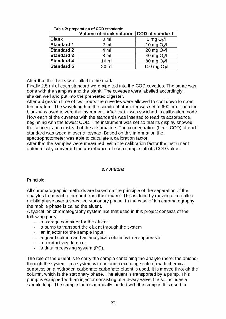
Table 2: preparation of COD standards

Volume of stock solution COD of standard

Blank 0 ml 0 mg O2/l

Standard 1 2 ml 10 mg O2/l

Standard 2 4 ml 20 mg O2/l

Standard 3 8 ml 40 mg O2/l

Standard 4 16 ml 80 mg O2/l

Standard 5 30 ml 150 mg O2/l

After that the flasks were filled to the mark.

Finally 2,5 ml of each standard were pipetted into the COD cuvettes. The same was

done with the samples and the blank. The cuvettes were labelled accordingly,

shaken well and put into the preheated digester.

After a digestion time of two hours the cuvettes were allowed to cool down to room

temperature. The wavelength of the spectrophotometer was set to 600 nm. Then the

blank was used to zero the instrument. After that it was switched to calibration mode.

Now each of the cuvettes with the standards was inserted to read its absorbance,

beginning with the lowest COD. The instrument was set so that its display showed

the concentration instead of the absorbance. The concentration (here: COD) of each

standard was typed in over a keypad. Based on this information the

spectrophotometer was able to calculate a calibration factor.

After that the samples were measured. With the calibration factor the instrument

automatically converted the absorbance of each sample into its COD value.

3.7 Anions

Principle:

All chromatographic methods are based on the principle of the separation of the

analytes from each other and from their matrix. This is done by moving a so-called

mobile phase over a so-called stationary phase. In the case of ion chromatography

the mobile phase is called the eluent.

A typical ion chromatography system like that used in this project consists of the

following parts:

- a storage container for the eluent

- a pump to transport the eluent through the system

- an injector for the sample input

- a guard column and an analytical column with a suppressor

- a conductivity detector

- a data processing system (PC).

The role of the eluent is to carry the sample containing the analyte (here: the anions)

through the system. In a system with an anion exchange column with chemical

suppression a hydrogen carbonate-carbonate-eluent is used. It is moved through the

column, which is the stationary phase. The eluent is transported by a pump. This

pump is equipped with an injector consisting of a 6-way valve. It also includes a

sample loop. The sample loop is manually loaded with the sample. It is used to

23

ensure that always the same amount of sample (here: 25 µl) is injected into the

eluent flow. This is done automatically with the 6-way injection valve.

The anion exchange column is packed with a 9 ɛm diameter macroporous resin bead

consisting of ethylvinylbenzene crosslinked with 55% divinylbenzene. The anion

exchange layer of this substrate is functionalised with quarternary ammonium groups.

The guard column installed prior to the analytical column consists of the same

components. It is there to prevent the elution of sample contaminants onto the

analytical column because it is easier to clean or replace the guard column.

The separation of the anions is based on the principle that they interact with the

stationary phase. Because of their different sizes and charges they pass the column

with different speeds. That means that every anion has a specific retention time,

according to its size and charge. For that reason the elution of the anions occurs in

the following order: fluoride, chloride, nitrite, bromide, nitrate, phosphate, and

sulphate. They are detected by a conductivity detector.

The electrolytic suppressor is a can be seen as a part of the detector. A suppressor

system has two major functions. The first one is to decrease the high basic

conductivity of the eluent to get a better signal-to-noise-ratio. The second one is to

convert the anions to be analysed into a stronger conducting form. This is achieved

by cation exchange processes in the suppressor. The eluent consists of the salts of

weakly dissociated acids, for example sodium hydrogen carbonate. The cation

exchange processes convert it into carbonic acid, which is a weak acid and poorly

dissociated so that its residual conductivity is also low. The anions to be determined,

for example chloride, are also converted into the free acid form, for example

hydrochloric acid, which has a higher conductivity than the salt.

By this suppression technique the sensitivity of detection is significantly increased.

The signal of the detection is plotted against the time. This results in a single peak for

every anion in the sample. The peaks are assigned by the order of the elution of the

anions, as explained above.

Ion chromatography is also a quantitative method. The peak area is directly

proportional to the concentration of the respective ion. With a set of standard

solutions of known anion concentrations one can create a calibration curve so that

the concentrations of the anions in a sample can be calculated (Lippold et al., 2002;

Dionex, 2005).

24

Material and chemicals:

- Ion chromatography system ICS-1000; Dionex, USA

- Guard column IonPac AG14, 4x50mm; Dionex, USA

- Analytical column IonPac AS14, 4x250mm; Dionex, USA

- Atlas electrolytic suppressor; Dionex, USA

- DS6 heated conductivity cell; Dionex, USA

- Software Chromeleon6; Dionex, USA

- Spatula

- Analytical balance

- Volumetric flasks, 100 ml, 1000 ml, 2000 ml; Brandt, Germany

- Eppendorf pipettes, 100 µl, 1000 µl, 5000 µl; Eppendorf, Germany

- Beakers; Schott Duran, Germany

- Syringe

- Deionised water (H2O)

- Sodium carbonate (Na2CO3)

- Sodium hydrogen carbonate (NaHCO3)

- Sodium fluoride (NaF), dried

- Sodium chloride (NaCl), dried

- Sodium bromide (NaBr), dried

- Sodium nitrate (NaNO3), dried

- Sodium nitrite (NaNO2), dried

- Potassium hydrogen phosphate (KH2PO4), dried

- Sodium phosphate (Na2SO4), dried

Performance:

The eluent was prepared by dissolving 21.2 g Na2CO3 and 2.1 g NaHCO3 in 250 ml

H2O. This solution was the eluent concentrate with a concentration of 0.8 mol/l for

Na2CO3 and 0.1 mol/l for NaHCO3. From this concentrate 20 ml were pipetted into a

2000 ml volumetric flask and it was filled to the mark with H2O. This diluted eluent

was filled into the eluent storage container of the IC system.

The eluent lasted for approximately three weeks, depending on the number of

samples measured.

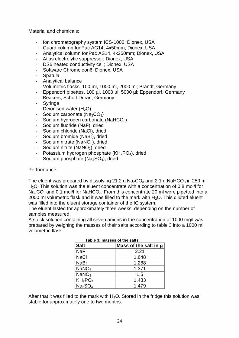
A stock solution containing all seven anions in the concentration of 1000 mg/l was

prepared by weighing the masses of their salts according to table 3 into a 1000 ml

volumetric flask.

Table 3: masses of the salts

Salt Mass of the salt in g

NaF 2.21

NaCl 1.648

NaBr 1.288

NaNO3 1.371

NaNO2 1.5

KH2PO4 1.433

Na2SO4 1.479

After that it was filled to the mark with H2O. Stored in the fridge this solution was

stable for approximately one to two months.

25

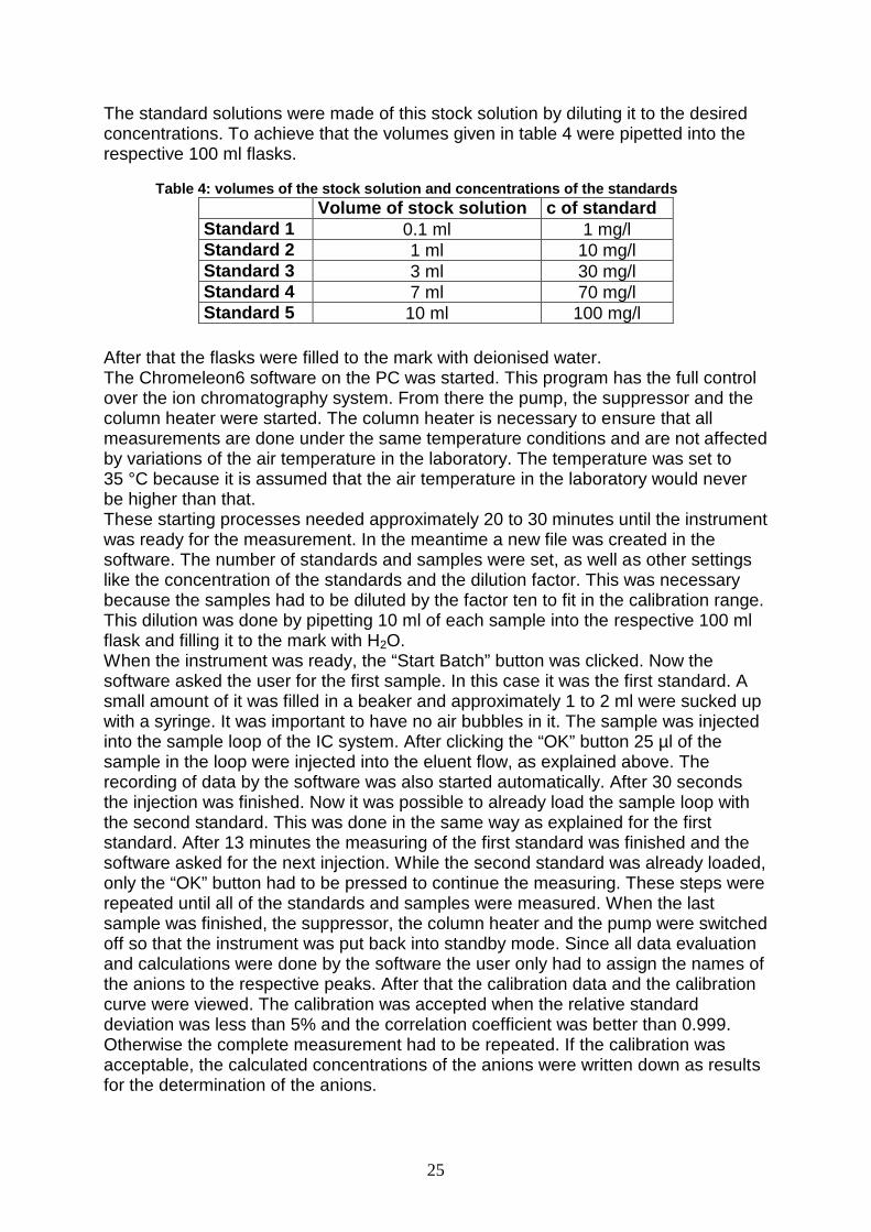
The standard solutions were made of this stock solution by diluting it to the desired

concentrations. To achieve that the volumes given in table 4 were pipetted into the

respective 100 ml flasks.

Table 4: volumes of the stock solution and concentrations of the standards

Volume of stock solution c of standard

Standard 1 0.1 ml 1 mg/l

Standard 2 1 ml 10 mg/l

Standard 3 3 ml 30 mg/l

Standard 4 7 ml 70 mg/l

Standard 5 10 ml 100 mg/l

After that the flasks were filled to the mark with deionised water.

The Chromeleon6 software on the PC was started. This program has the full control

over the ion chromatography system. From there the pump, the suppressor and the

column heater were started. The column heater is necessary to ensure that all

measurements are done under the same temperature conditions and are not affected

by variations of the air temperature in the laboratory. The temperature was set to

35 °C because it is assumed that the air temperature in the laboratory would never

be higher than that.

These starting processes needed approximately 20 to 30 minutes until the instrument

was ready for the measurement. In the meantime a new file was created in the

software. The number of standards and samples were set, as well as other settings

like the concentration of the standards and the dilution factor. This was necessary

because the samples had to be diluted by the factor ten to fit in the calibration range.

This dilution was done by pipetting 10 ml of each sample into the respective 100 ml

flask and filling it to the mark with H2O.

When the instrument was ready, the “Start Batch” button was clicked. Now the

software asked the user for the first sample. In this case it was the first standard. A

small amount of it was filled in a beaker and approximately 1 to 2 ml were sucked up

with a syringe. It was important to have no air bubbles in it. The sample was injected

into the sample loop of the IC system. After clicking the “OK” button 25 µl of the

sample in the loop were injected into the eluent flow, as explained above. The

recording of data by the software was also started automatically. After 30 seconds

the injection was finished. Now it was possible to already load the sample loop with

the second standard. This was done in the same way as explained for the first

standard. After 13 minutes the measuring of the first standard was finished and the

software asked for the next injection. While the second standard was already loaded,

only the “OK” button had to be pressed to continue the measuring. These steps were

repeated until all of the standards and samples were measured. When the last

sample was finished, the suppressor, the column heater and the pump were switched

off so that the instrument was put back into standby mode. Since all data evaluation

and calculations were done by the software the user only had to assign the names of

the anions to the respective peaks. After that the calibration data and the calibration

curve were viewed. The calibration was accepted when the relative standard

deviation was less than 5% and the correlation coefficient was better than 0.999.

Otherwise the complete measurement had to be repeated. If the calibration was

acceptable, the calculated concentrations of the anions were written down as results

for the determination of the anions.

26

3.8 Ammonia-nitrogen

First it has to be mentioned that originally an electrochemical method using an ion-

selective electrode was planned to be used for the determination of the ammonia-

nitrogen. The required equipment had to be ordered. Unfortunately delivery problems

occurred so that this equipment did not arrive during the time of this project. Finally

the determinations were done at the laboratory of the Buffalo City Municipality in East

London.

Principle:

The method used in this laboratory is a classical wet chemistry method, which forms

a good contrast towards the other modern methods used in this project. It is called

Nesslerisation or Nessler´s Method. This method is named after its developer, Julius

Nessler (1827 – 1905). In 1856 he showed a method for the determination of

ammonia using a special reagent, which is now known as Nessler´s reagent. This

reagent is an alkaline solution of potassium tetraiodomercurate(II). It reacts with

ammonia to form a yellowish-brown complex of polymeric nitrido-mercury(II)-iodide,

which is the iodide of the so-called Millon´s Base.

2 [HgI4]2-

+ 3 OH-

+ NH3 → [NHg2]I * H2O + 7 I-

+ 2 H2O

While the intensity of the colour is directly proportional to the concentration of the

ammonia-nitrogen, a sample can be measured spectrophotometrically against a set

of standard solutions with known amounts of ammonia-nitrogen (Wikipedia, 2005).

It has to be mentioned that this method is old and has been replaced by other

methods in many laboratories. This has mainly ecological reasons because mercury

compounds are highly toxic so that they cause severe disposal problems. Therefore

this method is not mentioned any more in the newer versions of the Standard

Methods for the examination of water and wastewater (Standard Methods, 1998).

Materials and chemicals:

- Distillation apparatus

- Volumetric flasks, 200 ml

- Test tubes

- Volumetric pipettes

- LKB Biochrom 4049 spectrophotometer

- Potassium hydroxide

- Nessler´s reagent

- 5% sodium hydroxide solution

27

Performance:

The determination of ammonia-nitrogen with the Nessler method is a routine analysis

in the laboratory of the Buffalo City Municipality. Therefore all needed solutions were

already prepared and ready to use and the spectrophotometer was also already

calibrated for the determination of ammonia-nitrogen.

First 500 ml of each sample were filled in the respective distillation apparatus and

boiled together with a spatula of potassium hydroxide. The ammonia in the sample

was converted into the gaseous form (NH3) under these basic conditions. The gas

escaped from the sample so that it was enriched in the distillate, where it was

dissolved again. The distillate was caught in 200 ml volumetric flasks.

This distillation step was done to concentrate the ammonia-nitrogen so that also low

concentrations can be determined. Considering that 500 ml were taken and

concentrated to 200 ml leads to the conclusion that the ammonia-nitrogen

concentration was increased by the factor 2.5.

After this step 20 ml of the concentrated sample were pipetted into a test tube. Then

1 ml of Nessler´s reagent and 5 ml of the 5% sodium hydroxide solution were added.

This was done with every sample. A blank was also prepared in the same way, with

deionised water instead of the sample. After a reaction time of 15 minutes the

spectrophotometer was zeroed with the blank and after that the absorbance of each

sample was read at a wavelength of 445 nm. As mentioned above, this method is

routine in this laboratory and therefore the staff members provided a factor to convert

the absorbance into the concentration of ammonia-nitrogen. This factor, being 3.67,

included the calibration data as well as the concentration factor mentioned above so

that no further calculations were necessary.

28

4. Results

During this project many samples have been taken and many parameters have been

determined. That leads to a large amount of results. It was decided that only average

values for the different parameters and sampling sites are shown here so that the

reader is not confused by big tables with hundreds of similar numerals. Only

interesting results, which help to achieve the aims of this project, are shown in more

detail. But nevertheless the appendix to this report provides tables with all exact

results for each sample and parameter so that these data are still accessible.

4.1 Appearance and smell

The influent sample taken from the balancing tank had a high turbidity, which was

visible to the human eye. This was caused by the organic matter and other colloids in

the wastewater. After the treatment steps the water was visibly clear. There are two

main reasons for that. The first one is that the suspended solids in the water settle

down on the surface of the material in the bioreactors. That is essential for the

purification process, as explained in the introduction. The second reason is that the

bacteria in these biofilms decompose the organic matter.

Another significant change of the water was the smell. The influent sample had an

offensive odour, mainly caused by gases like methane, hydrogen sulphide and

ammonia. These were removed by oxidation reactions carried out by the bacteria.

The decreasing intensity of the smell was noticeable from the first bioreactor on, and

the final effluent in the clarifier had no noticeable smell.

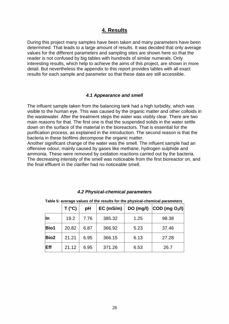
4.2 Physical-chemical parameters

Table 5: average values of the results for the physical-chemical parameters

T (°C) pH EC (mS/m) DO (mg/l) COD (mg O2/l)

In 19.2 7.76 385.32 1.25 98.38

Bio1 20.82 6.87 366.92 5.23 37.46

Bio2 21.21 6.95 366.15 6.13 27.28

Eff 21.12 6.95 371.26 6.53 26.7

29

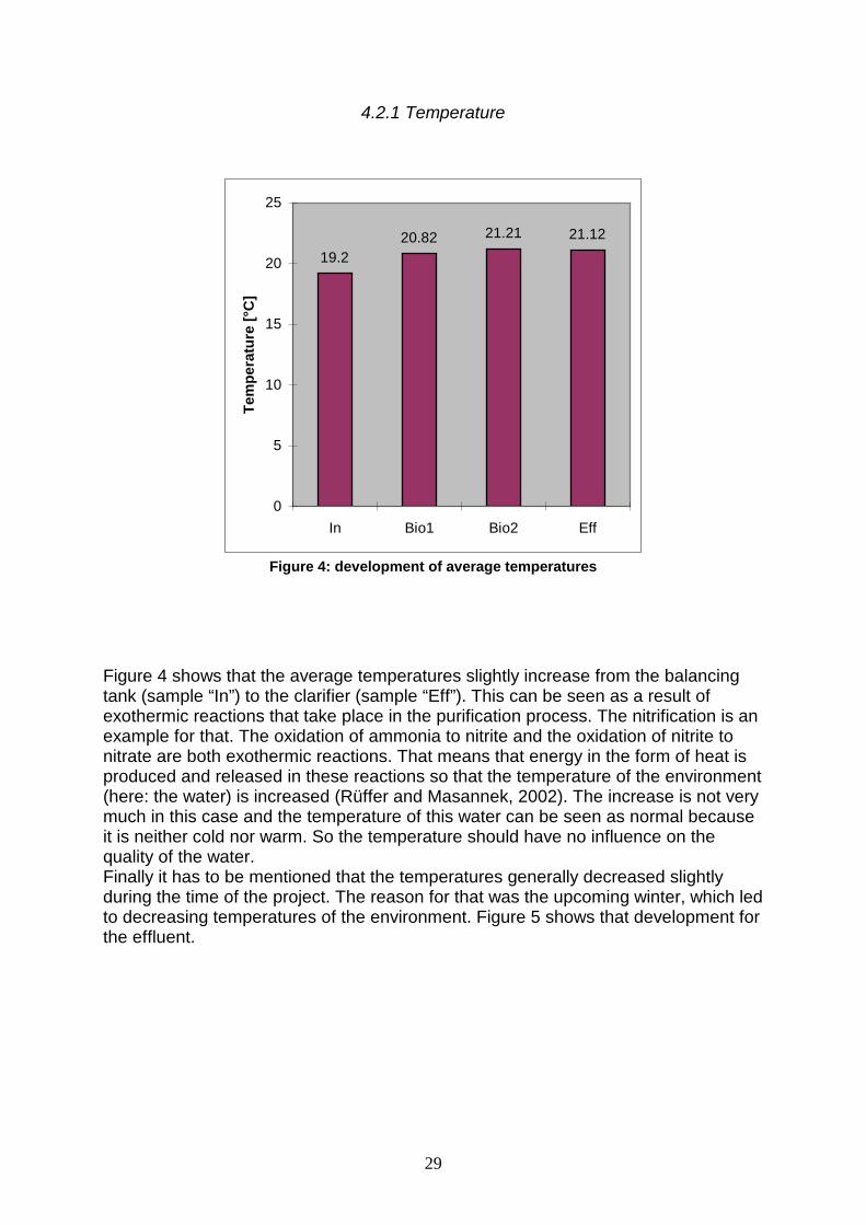
4.2.1 Temperature

19.2

20.8221.21 21.12

0

5

10

15

20

25

In Bio1 Bio2 Eff

Te

mp

era

ture

[°C

]

Figure 4: development of average temperatures

Figure 4 shows that the average temperatures slightly increase from the balancing

tank (sample “In”) to the clarifier (sample “Eff”). This can be seen as a result of

exothermic reactions that take place in the purification process. The nitrification is an

example for that. The oxidation of ammonia to nitrite and the oxidation of nitrite to

nitrate are both exothermic reactions. That means that energy in the form of heat is

produced and released in these reactions so that the temperature of the environment

(here: the water) is increased (Rüffer and Masannek, 2002). The increase is not very

much in this case and the temperature of this water can be seen as normal because

it is neither cold nor warm. So the temperature should have no influence on the

quality of the water.

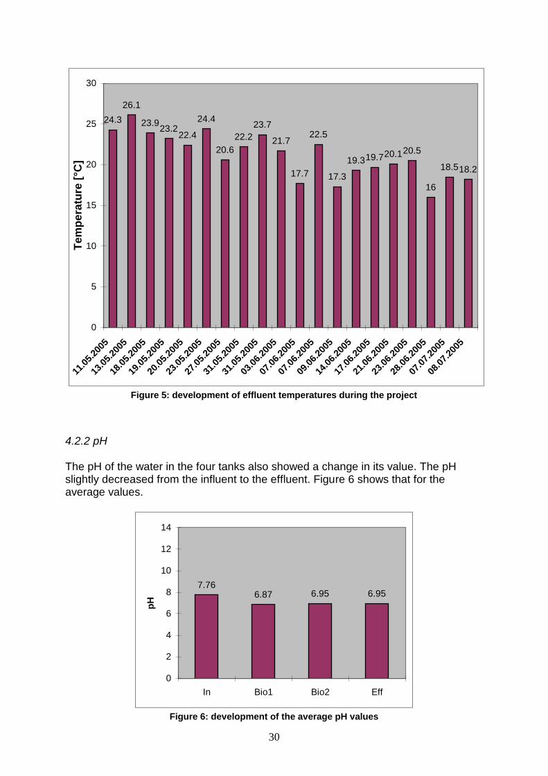
Finally it has to be mentioned that the temperatures generally decreased slightly

during the time of the project. The reason for that was the upcoming winter, which led

to decreasing temperatures of the environment. Figure 5 shows that development for

the effluent.

30

24.3

26.1

23.9

23.2

22.4

24.4

20.6

22.2

23.7

21.7

17.7

22.5

17.3

19.319.7

20.120.5

16

18.518.2

0

5

10

15

20

25

30

11.0

5.2

005

13.0

5.2

005

18.0

5.2

005

19.0

5.2

005

20.0

5.2

005

23.0

5.2

005

27.0

5.2

005

31.0

5.2

005

31.0

5.2

005

03.0

6.2

005

07.0

6.2

005

07.0

6.2

005

09.0

6.2

005

14.0

6.2

005

17.0

6.2

005

21.0

6.2

005

23.0

6.2

005

28.0

6.2

005

07.0

7.2

005

08.0

7.2

005

Te

mp

era

ture

[°C

]

Figure 5: development of effluent temperatures during the project

4.2.2 pH

The pH of the water in the four tanks also showed a change in its value. The pH

slightly decreased from the influent to the effluent. Figure 6 shows that for the

average values.

7.76

6.87 6.95 6.95

0

2

4

6

8

10

12

14

In Bio1 Bio2 Eff

pH

Figure 6: development of the average pH values

31

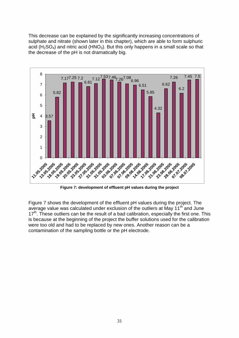
This decrease can be explained by the significantly increasing concentrations of

sulphate and nitrate (shown later in this chapter), which are able to form sulphuric

acid (H2SO4) and nitric acid (HNO3). But this only happens in a small scale so that

the decrease of the pH is not dramatically big.

3.57

5.82

7.177.25 7.2

6.81

7.126.96

6.51

5.85

4.32

6.62

7.26

6.2

7.57.457.08

7.267.467.53

0

1

2

3

4

5

6

7

8

11.0

5.2

005

13.0

5.2

005

18.0

5.2

005

19.0

5.2

005

20.0

5.2

005

23.0

5.2

005

27.0

5.2

005

31.0

5.2

005

31.0

5.2

005

03.0

6.2

005

07.0

6.2

005

07.0

6.2

005

09.0

6.2

005

14.0

6.2

005

17.0

6.2

005

21.0

6.2

005

23.0

6.2

005

28.0

6.2

005

07.0

7.2

005

08.0

7.2

005

pH

Figure 7: development of effluent pH values during the project

Figure 7 shows the development of the effluent pH values during the project. The

average value was calculated under exclusion of the outliers at May 11th

and June

17th

. These outliers can be the result of a bad calibration, especially the first one. This

is because at the beginning of the project the buffer solutions used for the calibration

were too old and had to be replaced by new ones. Another reason can be a

contamination of the sampling bottle or the pH electrode.

32

4.2.3 Electrical conductivity

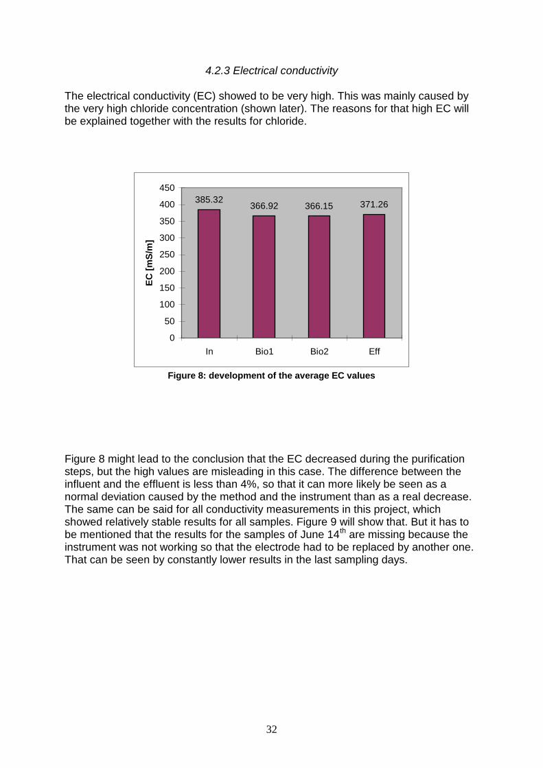
The electrical conductivity (EC) showed to be very high. This was mainly caused by

the very high chloride concentration (shown later). The reasons for that high EC will

be explained together with the results for chloride.

385.32

366.92 366.15 371.26

0

50

100

150

200

250

300

350

400

450

In Bio1 Bio2 Eff

EC

[m

S/m

]

Figure 8: development of the average EC values

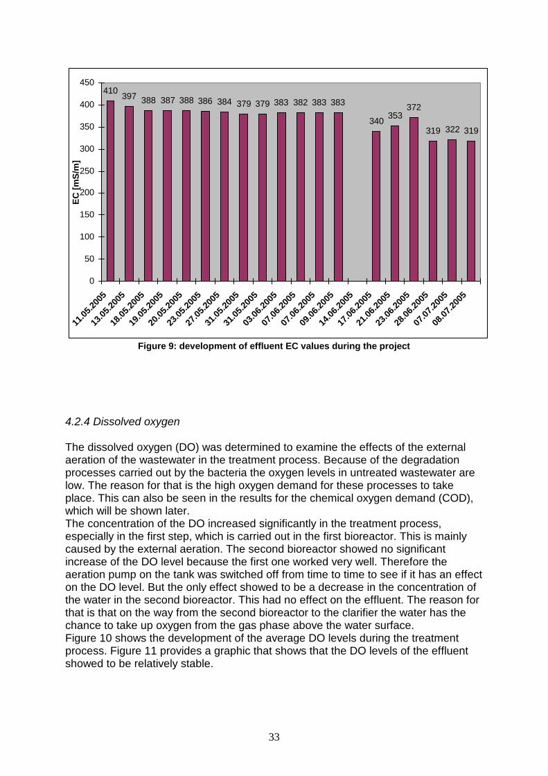
Figure 8 might lead to the conclusion that the EC decreased during the purification

steps, but the high values are misleading in this case. The difference between the

influent and the effluent is less than 4%, so that it can more likely be seen as a

normal deviation caused by the method and the instrument than as a real decrease.

The same can be said for all conductivity measurements in this project, which

showed relatively stable results for all samples. Figure 9 will show that. But it has to

be mentioned that the results for the samples of June 14th

are missing because the

instrument was not working so that the electrode had to be replaced by another one.

That can be seen by constantly lower results in the last sampling days.

33

410

397388 387 388 386 384

379 379 383 382 383 383

340

353

372

319 322 319

0

50

100

150

200

250

300

350

400

450

11.0

5.2

005

13.0

5.2

005

18.0

5.2

005

19.0

5.2

005

20.0

5.2

005

23.0

5.2

005

27.0

5.2

005

31.0

5.2

005

31.0

5.2

005

03.0

6.2

005

07.0

6.2

005

07.0

6.2

005

09.0

6.2

005

14.0

6.2

005

17.0

6.2

005

21.0

6.2

005

23.0

6.2

005

28.0

6.2

005

07.0

7.2

005

08.0

7.2

005

EC

[m

S/m

]

Figure 9: development of effluent EC values during the project

4.2.4 Dissolved oxygen

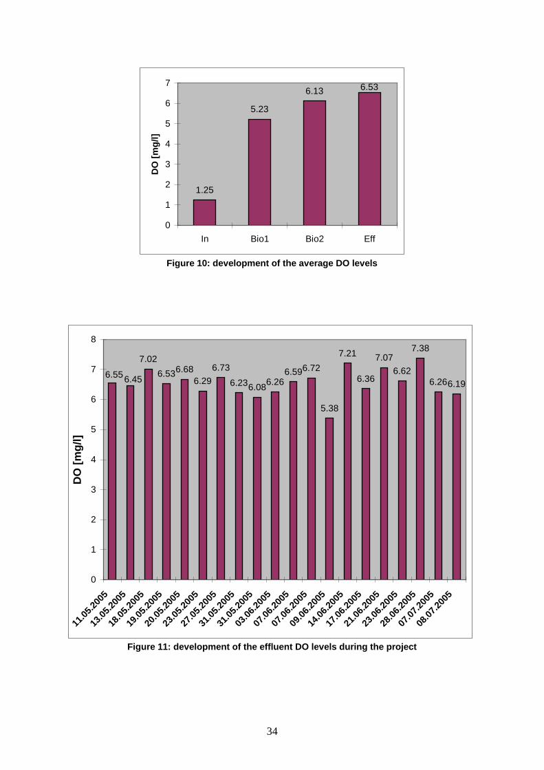
The dissolved oxygen (DO) was determined to examine the effects of the external

aeration of the wastewater in the treatment process. Because of the degradation

processes carried out by the bacteria the oxygen levels in untreated wastewater are

low. The reason for that is the high oxygen demand for these processes to take

place. This can also be seen in the results for the chemical oxygen demand (COD),

which will be shown later.

The concentration of the DO increased significantly in the treatment process,

especially in the first step, which is carried out in the first bioreactor. This is mainly

caused by the external aeration. The second bioreactor showed no significant

increase of the DO level because the first one worked very well. Therefore the

aeration pump on the tank was switched off from time to time to see if it has an effect

on the DO level. But the only effect showed to be a decrease in the concentration of

the water in the second bioreactor. This had no effect on the effluent. The reason for

that is that on the way from the second bioreactor to the clarifier the water has the

chance to take up oxygen from the gas phase above the water surface.

Figure 10 shows the development of the average DO levels during the treatment

process. Figure 11 provides a graphic that shows that the DO levels of the effluent

showed to be relatively stable.

34

1.25

5.23

6.136.53

0

1

2

3

4

5

6

7

In Bio1 Bio2 Eff

DO

[m

g/l]

Figure 10: development of the average DO levels

7.02

6.536.68

6.29

6.73

6.236.08

6.26

6.596.72

5.38

7.21

6.36

7.07

6.62

7.38

6.266.196.45

6.55

0

1

2

3

4

5

6

7

8

11.0

5.2

005

13.0

5.2

005

18.0

5.2

005

19.0

5.2

005

20.0

5.2

005

23.0

5.2

005

27.0

5.2

005

31.0

5.2

005

31.0

5.2

005

03.0

6.2

005

07.0

6.2

005

07.0

6.2

005

09.0

6.2

005

14.0

6.2

005

17.0

6.2

005

21.0

6.2

005

23.0

6.2

005

28.0

6.2

005

07.0

7.2

005

08.0

7.2

005

DO

[m

g/l

]

Figure 11: development of the effluent DO levels during the project

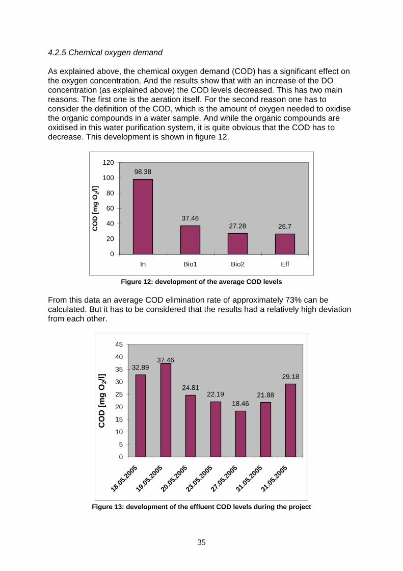
35

4.2.5 Chemical oxygen demand

As explained above, the chemical oxygen demand (COD) has a significant effect on

the oxygen concentration. And the results show that with an increase of the DO

concentration (as explained above) the COD levels decreased. This has two main

reasons. The first one is the aeration itself. For the second reason one has to

consider the definition of the COD, which is the amount of oxygen needed to oxidise

the organic compounds in a water sample. And while the organic compounds are

oxidised in this water purification system, it is quite obvious that the COD has to

decrease. This development is shown in figure 12.

98.38

37.46

27.28 26.7

0

20

40

60

80

100

120

In Bio1 Bio2 Eff

CO

D [

mg

O2/l]

Figure 12: development of the average COD levels

From this data an average COD elimination rate of approximately 73% can be

calculated. But it has to be considered that the results had a relatively high deviation

from each other.

32.89

24.81

22.19

18.46

21.88

29.18

37.46

0

5

10

15

20

25

30

35

40

45

18.0

5.2

005

19.0

5.2

005

20.0

5.2

005

23.0

5.2

005

27.0

5.2

005

31.0

5.2

005

31.0

5.2

005

CO

D [

mg

O2/l

]

Figure 13: development of the effluent COD levels during the project

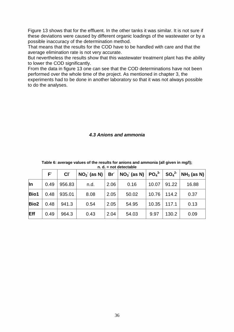
36

Figure 13 shows that for the effluent. In the other tanks it was similar. It is not sure if

these deviations were caused by different organic loadings of the wastewater or by a

possible inaccuracy of the determination method.

That means that the results for the COD have to be handled with care and that the

average elimination rate is not very accurate.

But nevertheless the results show that this wastewater treatment plant has the ability

to lower the COD significantly.

From the data in figure 13 one can see that the COD determinations have not been

performed over the whole time of the project. As mentioned in chapter 3, the

experiments had to be done in another laboratory so that it was not always possible

to do the analyses.

4.3 Anions and ammonia

Table 6: average values of the results for anions and ammonia (all given in mg/l);

n. d. = not detectable

F-

Cl-

NO2

- (as N) Br

-NO3

- (as N) PO4

3-SO4

2-NH3 (as N)

In 0.49 956.83 n.d. 2.06 0.16 10.07 91.22 16.88

Bio1 0.48 935.01 8.08 2.05 50.02 10.76 114.2 0.37

Bio2 0.48 941.3 0.54 2.05 54.95 10.35 117.1 0.13

Eff 0.49 964.3 0.43 2.04 54.03 9.97 130.2 0.09

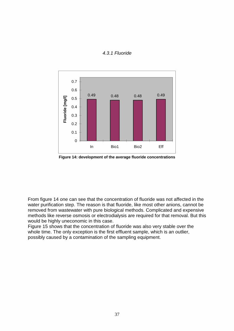
37

4.3.1 Fluoride

0.49 0.48 0.48 0.49

0

0.1

0.2

0.3

0.4

0.5

0.6

0.7

In Bio1 Bio2 Eff

Flu

orid

e [

mg

/l]

Figure 14: development of the average fluoride concentrations

From figure 14 one can see that the concentration of fluoride was not affected in the

water purification step. The reason is that fluoride, like most other anions, cannot be

removed from wastewater with pure biological methods. Complicated and expensive

methods like reverse osmosis or electrodialysis are required for that removal. But this

would be highly uneconomic in this case.

Figure 15 shows that the concentration of fluoride was also very stable over the

whole time. The only exception is the first effluent sample, which is an outlier,

possibly caused by a contamination of the sampling equipment.

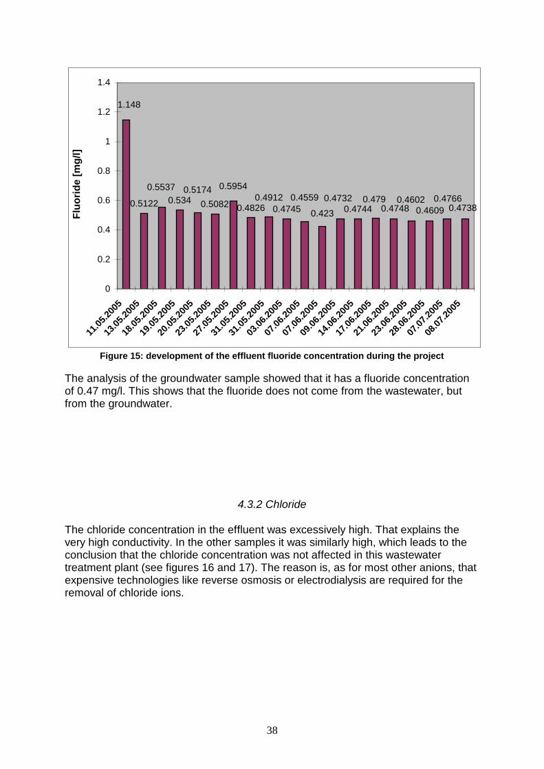
38

0.51220.534

0.4826 0.4745 0.4744

0.47660.46020.479

0.51740.5537

0.5082

0.4912 0.4732

1.148

0.5954

0.4559

0.4230.4748 0.4609

0.4738

0

0.2

0.4

0.6

0.8

1

1.2

1.4

11.0

5.2

005

13.0

5.2

005

18.0

5.2

005

19.0

5.2

005

20.0

5.2

005

23.0

5.2

005

27.0

5.2

005

31.0

5.2

005

31.0

5.2

005

03.0

6.2

005

07.0

6.2

005

07.0

6.2

005

09.0

6.2

005

14.0

6.2

005

17.0

6.2

005

21.0

6.2

005

23.0

6.2

005

28.0

6.2

005

07.0

7.2

005

08.0

7.2

005

Flu

orid

e [

mg

/l]

Figure 15: development of the effluent fluoride concentration during the project

The analysis of the groundwater sample showed that it has a fluoride concentration

of 0.47 mg/l. This shows that the fluoride does not come from the wastewater, but

from the groundwater.

4.3.2 Chloride

The chloride concentration in the effluent was excessively high. That explains the

very high conductivity. In the other samples it was similarly high, which leads to the

conclusion that the chloride concentration was not affected in this wastewater

treatment plant (see figures 16 and 17). The reason is, as for most other anions, that

expensive technologies like reverse osmosis or electrodialysis are required for the

removal of chloride ions.

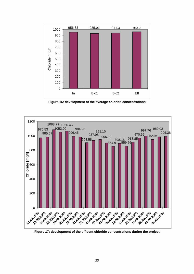
39

941.3935.01956.83 964.3

0

100

200

300

400

500

600

700

800

900

1000

In Bio1 Bio2 Eff

Ch

lorid

e [

mg

/l]

Figure 16: development of the average chloride concentrations

985.67

1053.00

996.45

898.18

859.26

913.85

970.69952.94

996.38

997.76

905.13

937.95

951.10

1066.46

989.03

854.91

908.58

984.26

1088.79

975.53

0

200

400

600

800

1000

1200

11.0

5.2

005

13.0

5.2

005

18.0

5.2

005

19.0

5.2

005

20.0

5.2

005

23.0

5.2

005

27.0

5.2

005

31.0

5.2

005

31.0

5.2

005

03.0

6.2

005

07.0

6.2

005

07.0

6.2

005

09.0

6.2

005

14.0

6.2

005

17.0

6.2

005

21.0

6.2

005

23.0

6.2

005

28.0

6.2

005

07.0

7.2

005

08.0

7.2

005

Ch

lorid

e [

mg

/l]

Figure 17: development of the effluent chloride concentrations during the project

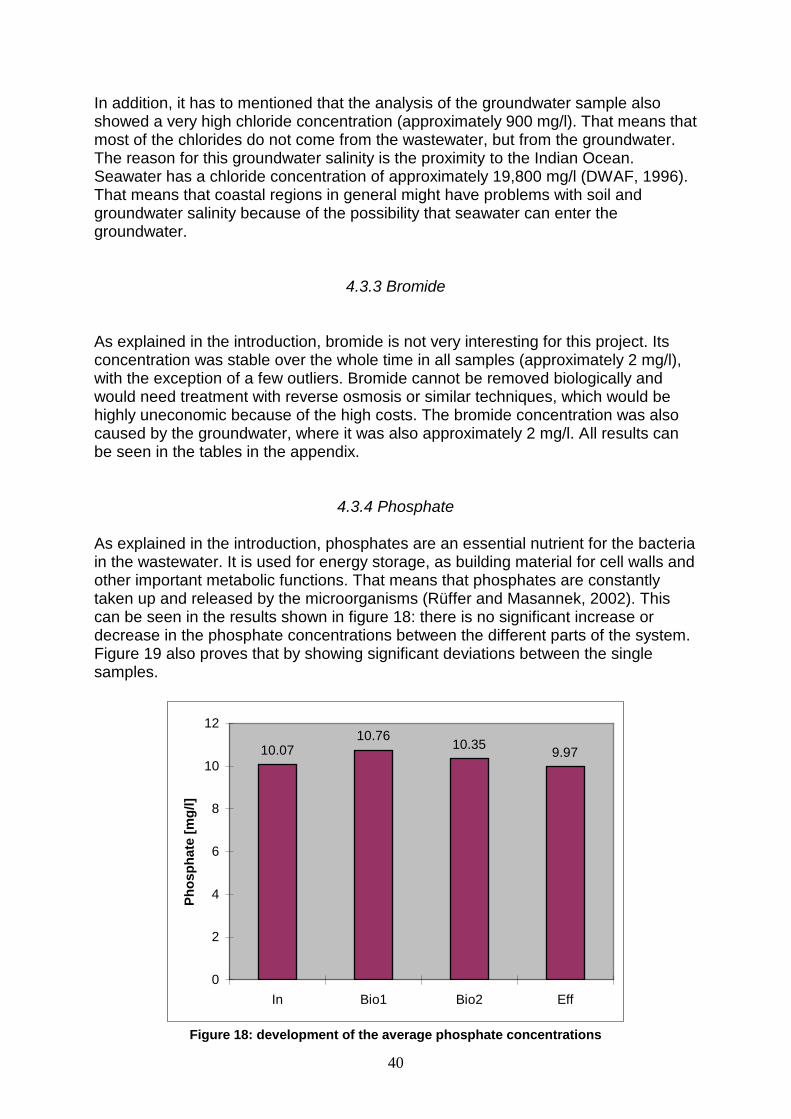
40

In addition, it has to mentioned that the analysis of the groundwater sample also

showed a very high chloride concentration (approximately 900 mg/l). That means that

most of the chlorides do not come from the wastewater, but from the groundwater.

The reason for this groundwater salinity is the proximity to the Indian Ocean.

Seawater has a chloride concentration of approximately 19,800 mg/l (DWAF, 1996).

That means that coastal regions in general might have problems with soil and

groundwater salinity because of the possibility that seawater can enter the

groundwater.

4.3.3 Bromide

As explained in the introduction, bromide is not very interesting for this project. Its

concentration was stable over the whole time in all samples (approximately 2 mg/l),

with the exception of a few outliers. Bromide cannot be removed biologically and

would need treatment with reverse osmosis or similar techniques, which would be

highly uneconomic because of the high costs. The bromide concentration was also

caused by the groundwater, where it was also approximately 2 mg/l. All results can

be seen in the tables in the appendix.

4.3.4 Phosphate

As explained in the introduction, phosphates are an essential nutrient for the bacteria

in the wastewater. It is used for energy storage, as building material for cell walls and

other important metabolic functions. That means that phosphates are constantly

taken up and released by the microorganisms (Rüffer and Masannek, 2002). This

can be seen in the results shown in figure 18: there is no significant increase or

decrease in the phosphate concentrations between the different parts of the system.

Figure 19 also proves that by showing significant deviations between the single

samples.

10.07

10.76

10.35

9.97

0

2

4

6

8

10

12

In Bio1 Bio2 Eff

Ph

os

ph

ate

[m

g/l

]

Figure 18: development of the average phosphate concentrations

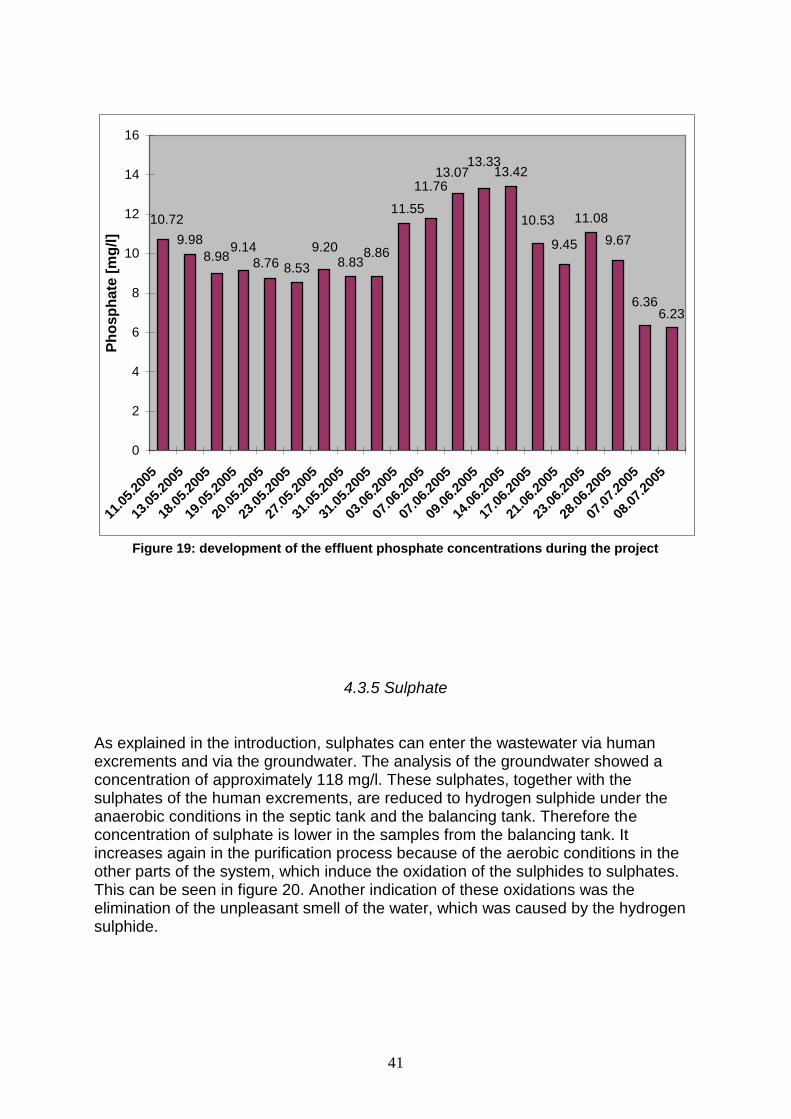
41

9.98

8.538.83

13.42

11.08

6.36

8.869.14

6.23

9.679.45

10.53

13.07

13.33

11.55

11.76

8.76

9.20

8.98

10.72

0

2

4

6

8

10

12

14

16

11.0

5.2

005

13.0

5.2

005

18.0

5.2

005

19.0

5.2

005

20.0

5.2

005

23.0

5.2

005

27.0

5.2

005

31.0

5.2

005

31.0

5.2

005

03.0

6.2

005

07.0

6.2

005

07.0

6.2

005

09.0

6.2

005

14.0

6.2

005

17.0

6.2

005

21.0

6.2

005

23.0

6.2

005

28.0

6.2

005

07.0

7.2

005

08.0

7.2

005

Ph

os

ph

ate

[m

g/l]

Figure 19: development of the effluent phosphate concentrations during the project

4.3.5 Sulphate

As explained in the introduction, sulphates can enter the wastewater via human

excrements and via the groundwater. The analysis of the groundwater showed a

concentration of approximately 118 mg/l. These sulphates, together with the

sulphates of the human excrements, are reduced to hydrogen sulphide under the

anaerobic conditions in the septic tank and the balancing tank. Therefore the

concentration of sulphate is lower in the samples from the balancing tank. It

increases again in the purification process because of the aerobic conditions in the

other parts of the system, which induce the oxidation of the sulphides to sulphates.

This can be seen in figure 20. Another indication of these oxidations was the

elimination of the unpleasant smell of the water, which was caused by the hydrogen

sulphide.

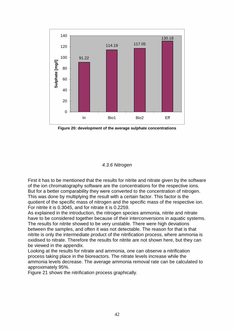
42

91.22

114.19117.05

130.18

0

20

40

60

80

100

120

140

In Bio1 Bio2 Eff

Su

lph

ate

[m

g/l]

Figure 20: development of the average sulphate concentrations

4.3.6 Nitrogen

First it has to be mentioned that the results for nitrite and nitrate given by the software

of the ion chromatography software are the concentrations for the respective ions.

But for a better comparability they were converted to the concentration of nitrogen.

This was done by multiplying the result with a certain factor. This factor is the

quotient of the specific mass of nitrogen and the specific mass of the respective ion.

For nitrite it is 0.3045, and for nitrate it is 0.2259.

As explained in the introduction, the nitrogen species ammonia, nitrite and nitrate

have to be considered together because of their interconversions in aquatic systems.

The results for nitrite showed to be very unstable. There were high deviations

between the samples, and often it was not detectable. The reason for that is that

nitrite is only the intermediate product of the nitrification process, where ammonia is

oxidised to nitrate. Therefore the results for nitrite are not shown here, but they can

be viewed in the appendix.

Looking at the results for nitrate and ammonia, one can observe a nitrification

process taking place in the bioreactors. The nitrate levels increase while the

ammonia levels decrease. The average ammonia removal rate can be calculated to

approximately 95%.

Figure 21 shows the nitrification process graphically.

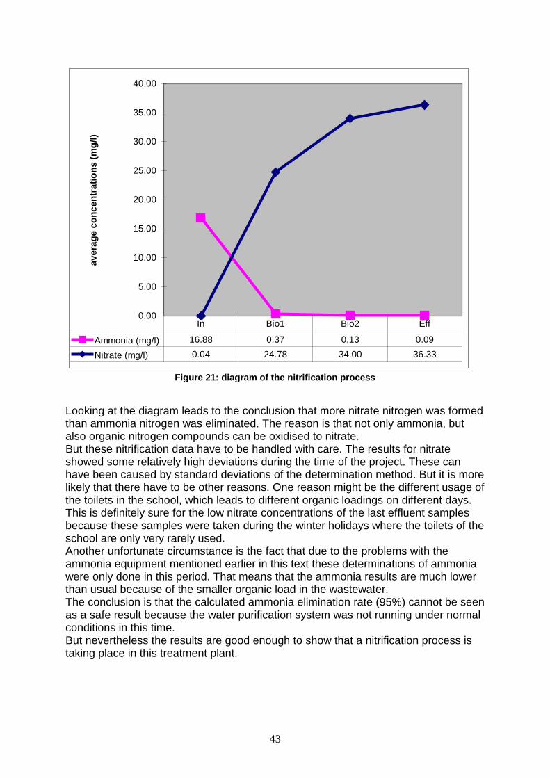
43

0.00

5.00

10.00

15.00

20.00

25.00

30.00

35.00

40.00

av

era

ge

co

nc

en

tra

tio

ns

(m

g/l)

Ammonia (mg/l) 16.88 0.37 0.13 0.09

Nitrate (mg/l) 0.04 24.78 34.00 36.33

In Bio1 Bio2 Eff

Figure 21: diagram of the nitrification process

Looking at the diagram leads to the conclusion that more nitrate nitrogen was formed

than ammonia nitrogen was eliminated. The reason is that not only ammonia, but

also organic nitrogen compounds can be oxidised to nitrate.

But these nitrification data have to be handled with care. The results for nitrate

showed some relatively high deviations during the time of the project. These can

have been caused by standard deviations of the determination method. But it is more

likely that there have to be other reasons. One reason might be the different usage of

the toilets in the school, which leads to different organic loadings on different days.

This is definitely sure for the low nitrate concentrations of the last effluent samples

because these samples were taken during the winter holidays where the toilets of the

school are only very rarely used.

Another unfortunate circumstance is the fact that due to the problems with the

ammonia equipment mentioned earlier in this text these determinations of ammonia

were only done in this period. That means that the ammonia results are much lower

than usual because of the smaller organic load in the wastewater.

The conclusion is that the calculated ammonia elimination rate (95%) cannot be seen

as a safe result because the water purification system was not running under normal

conditions in this time.

But nevertheless the results are good enough to show that a nitrification process is

taking place in this treatment plant.

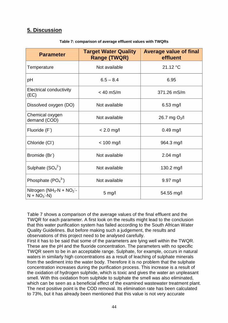
44

5. Discussion

Table 7: comparison of average effluent values with TWQRs

ParameterTarget Water Quality

Range (TWQR)

Average value of final

effluent

Temperature Not available 21.12 °C

pH 6.5 – 8.4 6.95

Electrical conductivity

(EC) < 40 mS/m 371.26 mS/m

Dissolved oxygen (DO) Not available 6.53 mg/l

Chemical oxygen

demand (COD)Not available 26.7 mg O2/l

Fluoride (F-

) < 2.0 mg/l 0.49 mg/l

Chloride (Cl-

) < 100 mg/l 964.3 mg/l

Bromide (Br-

) Not available 2.04 mg/l

Sulphate (SO4

2-

) Not available 130.2 mg/l

Phosphate (PO4

3-

) Not available 9.97 mg/l

Nitrogen (NH3-N + NO2

-

-

N + NO3

-

-N)5 mg/l 54.55 mg/l

Table 7 shows a comparison of the average values of the final effluent and the

TWQR for each parameter. A first look on the results might lead to the conclusion

that this water purification system has failed according to the South African Water

Quality Guidelines. But before making such a judgement, the results and

observations of this project need to be analysed carefully.

First it has to be said that some of the parameters are lying well within the TWQR.

These are the pH and the fluoride concentration. The parameters with no specific

TWQR seem to be in an acceptable range. Sulphate, for example, occurs in natural

waters in similarly high concentrations as a result of leaching of sulphate minerals

from the sediment into the water body. Therefore it is no problem that the sulphate

concentration increases during the purification process. This increase is a result of

the oxidation of hydrogen sulphide, which is toxic and gives the water an unpleasant

smell. With this oxidation from sulphide to sulphate the smell was also eliminated,

which can be seen as a beneficial effect of the examined wastewater treatment plant.

The next positive point is the COD removal. Its elimination rate has been calculated

to 73%, but it has already been mentioned that this value is not very accurate

45

because of the high deviations between the single results of the COD determinations.

Nevertheless it can be seen as good, compared to other treatment plants working

with the same principle. Some of them are working better and show COD elimination

rates of 92% (Sotirakou et al., 1999), but there are also treatment plants, which

remove only 60% of the COD (Garrido et al., 1998). Another South African project

with an anaerobic baffled reactor showed a COD elimination rate between 58% and

72% (Foxon et al., 2004). From this point of view the treatment plant at the Lilyfontein

School is successful, although the rate could be higher. It is suggested that further

analyses have to be performed to get more accurate results.

Another very significant effect of this submerged fixed-film bioreactor system is the

nitrification. The ammonia is almost completely eliminated in the purification process

(95%), which can be seen as a very good rate. Similar ammonia removal rates other

biological water purification systems are described in the literature (Verhoeven and

Meuleman, 1999; Oh et al., 2001; Ho et al., 2001; Lesjean et al., 2002; Cicek, 2003;

Foxon et al., 2004).

The biggest problem in the final effluent of this water purification system is the

excessively high chloride concentration, which also causes the very high electrical

conductivity (EC). It is caused by the groundwater, where these values are similarly

high because of the proximity to the ocean. The system cannot be held responsible

for that. Chloride, as well as most other ions, can only be removed with reverse

osmosis or similar techniques, which are characterised by the high costs. Therefore it

would be highly uneconomic to apply such techniques for the treatment of water,

which is intended to be used for irrigation. A farmer with saline irrigation water has

only two chances: he can either accept the reduced crop yield which might be caused

by that, or he has to switch to other plants and crops which are more tolerant towards

high chloride concentrations (DWAF, 1996).

In the case of the Lilyfontein School this problem does not occur because it is no

farm. The school has two big rugby fields, which are intended to be irrigated with the

treated wastewater. Only grass is growing on a normal sports field, and most grass

species are very tolerant towards high chloride concentrations (DWAF, 1996).

That means that the final effluent can still be used here as long as only the grass of

the rugby fields is irrigated with it.

But another problem of the final effluent is its high nitrate concentration, which also

exceeds the TWQR significantly. Nitrate is a key nutrient for plants and commercially

available fertilisers also contain nitrates. But if the concentration exceeds the

requirements of the plants, they cannot take up this excess of nitrate so that it can

contaminate the groundwater.

This problem can be solved by a process called denitrification where nitrate is

reduced to gaseous elemental nitrogen, which can escape to the atmosphere. This is

currently not happening in this fixed-film bioreactor. But with some technical

modifications according to conventional wastewater treatment plants in Germany this

denitrification step could be realised.

Denitrification requires anoxic conditions. The first idea would be to shut down the

aeration of the second bioreactor to create these conditions so that denitrification can

take place after the nitrification in the first bioreactor. But this is not practicable

because the bacteria responsible for that process also require organic compounds as

an energy source. But these have already been decomposed in the aerobic step of

the first bioreactor. It would be possible to add organic compounds, for example

methanol, to the water in the second tank, but this would be highly uneconomic. To

solve this problem, the system has to be modified. The first bioreactor has to become

the anoxic step and the second bioreactor has to become the aerobic step. Further a

46

pipe has to be installed so that a part of the water in the second reactor can flow

back to the first one. After doing that, the following should happen:

First the water flows through the anoxic part of the system where no significant

reactions occur so that the water is still rich in organic compounds. In the second

(aerated) reactor all the described reactions occur, which are sulphide oxidation,

COD removal and nitrification. Now a part of the nitrate-rich water is recirculated into

the first reactor where anoxic conditions and organic compounds can be found so

that the denitrification can take place. The water should have a low nitrate

concentration after that step. Then this water will travel through the second tank

again and can finally flow into the clarifier (Rüffer and Masannek, 2002).

This suggestion is only theoretical. But it should be tested in the following parts of this

project because a denitrification step is essential for the success of this water

purification system to produce water, which can be used for different purposes.

If these modifications would be successful, the nitrate levels would be lowered so that

the final effluent fits the TWQR set by the DWAF.

That leads to the next point. As described in chapter 2, the whole project has got the

aim to convince municipalities and governments of the applicability of these

decentralized water purification systems. This could lead to installations of such

systems on a bigger scale in rural areas and urban settlements, which are not

connected to the municipal sewage system. The result would be a better water

management so that the predicted water scarcity mentioned in the introduction might

be avoided.

But after this first part of the project it is hard to say if the system tested here can be

judged to be good or bad because there are good and bad results. The high chloride

concentration and the high conductivity are a local problem of this coastal region so

that this cannot be seen as a disadvantage of the treatment process.

But an advantage is the relatively good COD removal rate and the elimination of

unpleasant smells.

The only thing that has to be improved is the mentioned denitrification step. And it is

quite obvious that more parameters have to be determined in future projects. The

parameters tested here were quite important, but other parameters, for example the

biochemical oxygen demand (BOD), total suspended solids (TSS), turbidity, total

nitrogen, total phosphorous and biological parameters like E. coli and coliforms, have

to be added to the list. This is important because the only final judgement of the

effluent quality can be made on the base of a complete parameter list.

But, as mentioned above, this project was only a part of a bigger project. The results

can lead to the final conclusion that this decentralized water purification system

installed at the Lilyfontein School in the Eastern Cape of South Africa is working well

and that this technology, after the suggested modifications, has the ability to assist in

solving South Africa’s water problems to avoid the predicted water scarcity in 2025.

47

6. References

Literature sources in order of appearance

FAO – Food and Agriculture Organisation of the United Nations (2005):

AQUASTAT COUNTRY PROFILES, viewed at

http://www.fao.org/ag/agl/aglw/aquastat/countries/south_africa/index.stm

F.A.O. Otieno and G.M.M. Ochieng (2004): Water management tools as a means of

averting a possible water scarcity in South Africa by the year 2025

Water SA Vol. 30 No. 5 (Special Edition), 120-124

I. Nhapi and H.J. Gijzen (2005): A 3-step strategic approach to sustainable

wastewater management

Water SA Vol. 31 No. 1 (January 2005), 133-140

J.T.A. Verhoeven and A.F.M. Meuleman (1999): Wetlands for wastewater treatment:

Opportunities and limitations

Ecological Engineering 12 (1999), 5-12

K.M. Foxon, S. Pillay, T. Lalbahadur, N. Rodda, F. Holder and C.A. Buckley (2004):

The anaerobic baffled reactor (ABR): An appropriate technology for on-site sanitation

Water SA Vol. 30 No. 5 (Special Edition), 44-50

J. Oh, S.M. Yoon and J.M. Park (2001): Denitrification in submerged biofilters of

concentrated-nitrate wastewater

Water Science and Technology Vol. 43 No. 1, 217-223

C.M. Ho, S.K. Tseng and Y.J. Chang (2001): Autotrophic denitrification via a novel

membrane-attached biofilm reactor

Letters in Applied Microbiology 2001, 33, 201-205

B. Lesjean, R. Gnirss and C. Adam (2002): Process configurations adapted to

membrane bioreactors for enhanced biological phosphorous and nitrogen removal

Desalination 149 (2002), 217-224

N. Cicek (2003): A review of membrane bioreactors and their potential application in

the treatment of agricultural wastewater

Canadian Biosystems Engineering Volume 45, 6.37-6.49

M.T. Madigan, J.M. Martinko, J. Parker:

Brock Biology of Microorganisms, 10th

Edition, Upper Saddle River, NJ: Prentice Hall

2003

H. Rüffer and R. Masannek (2002): Abwasserreinigung zum Schutze der Gewässer

und ihrer Nutzbarkeit, in: A. Grohmann (editor): Karl Höll: Wasser:

Nutzung im Kreislauf, Hygiene, Analyse und Bewertung. 8. völlig neu bearbeitete

Auflage, Walter de Gruyter, Berlin, 833-902

48

J. Johnston and T. Smith (2005): An Introduction to Septic Tank Sewage Treatment

Systems, viewed at http://www.johnstonsmith.co.uk/fact4.html

CLEAREDGE (2005): Clearedge On-Site Effluent Treatment, viewed at

http://www.clearedgeprojects.com

DWAF - Department of Water Affairs and Forestry, 1996. South African Water Quality

Guidelines (second edition). Volume 4: Agricultural Use: Irrigation

A. Grohmann and W. Nissing (2002): Chemie des Wassers, in: A. Grohmann (editor):

Karl Höll: Wasser: Nutzung im Kreislauf, Hygiene, Analyse und Bewertung. 8. völlig

neu bearbeitete Auflage, Walter de Gruyter, Berlin, 55-57

STANDARD METHODS (1998): Standard methods for the examination of water and

wastewater, 20th

edition, American Public Health Association, Washington, D.C.

A. Grohmann, H.H. Dieter and H. Höring (2002): Befund und Bewertung, in: A.

Grohmann (editor): Karl Höll: Wasser: Nutzung im Kreislauf, Hygiene, Analyse und

Bewertung. 8. völlig neu bearbeitete Auflage, Walter de Gruyter, Berlin, 677-717

M. Otto (2000): Analytische Chemie, zweite, vollständig überarbeitete Auflage,

Wiley-VCH, Weinheim

E. Stottmeister (2002): Physikalische und physikalisch-chemische Untersuchungen,

in: A. Grohmann (editor): Karl Höll: Wasser: Nutzung im Kreislauf, Hygiene, Analyse

und Bewertung. 8. völlig neu bearbeitete Auflage, Walter de Gruyter, Berlin, 140-146

WTW (2005): Wissenschaftlich Technische Werkstätten, product catalogue,

viewed at http://www.wtw.de

U. Lippold, E. Stottmeister and R. Schuster (2002): Instrumentelle Methoden in der

Wasseranalytik, in: A. Grohmann (editor): Karl Höll: Wasser: Nutzung im Kreislauf,

Hygiene, Analyse und Bewertung. 8. völlig neu bearbeitete Auflage, Walter de

Gruyter, Berlin, 178-182 and 207-210

DIONEX (2005): Dionex corporation: technical data sheet and instruction manual for

ICS-1000, viewed at http://www.dionex.com

WIKIPEDIA (2005): Wikipedia, the free encyclopaedia: Nessler´s reagent,

viewed at http://en.wikipedia.org/wiki/Nessler's_reagent

E. Sotirakou, G. Kladitis, N. Diamantis, H. Grigoropoulou (1999): Ammonia and

phosphorus removal in municipal wastewater treatment plant with extended aeration

Global Nest: the Int. J. Vol. 1 No.1, 47-53

J.M. Garrido, L. Guerrero, R. Méndez and J.M. Lema (1998): Nitrification of waste

waters from fish-meal factories

Water SA Vol. 24 No. 3 (July 1998), 245-250

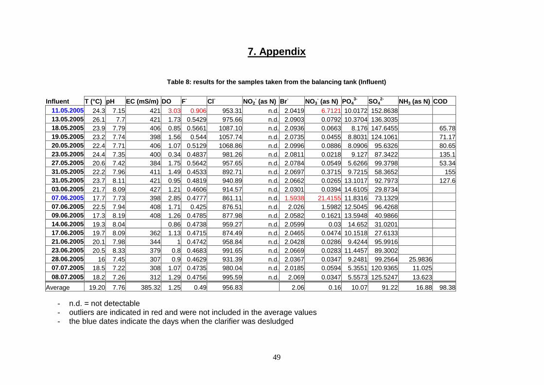
49

7. Appendix

Table 8: results for the samples taken from the balancing tank (Influent)

Influent T (°C) pH EC (mS/m) DO F-

Cl-

NO2

- (as N) Br

-NO3

- (as N) PO4

3-SO4

2-NH3 (as N) COD

11.05.2005 24.3 7.15 421 3.03 0.906 953.31 n.d. 2.0419 6.7121 10.0172 152.8638

13.05.2005 26.1 7.7 421 1.73 0.5429 975.66 n.d. 2.0903 0.0792 10.3704 136.3035

18.05.2005 23.9 7.79 406 0.85 0.5661 1087.10 n.d. 2.0936 0.0663 8.176 147.6455 65.78

19.05.2005 23.2 7.74 398 1.56 0.544 1057.74 n.d. 2.0735 0.0455 8.8031 124.1061 71.17

20.05.2005 22.4 7.71 406 1.07 0.5129 1068.86 n.d. 2.0996 0.0886 8.0906 95.6326 80.65

23.05.2005 24.4 7.35 400 0.34 0.4837 981.26 n.d. 2.0811 0.0218 9.127 87.3422 135.1

27.05.2005 20.6 7.42 384 1.75 0.5642 957.65 n.d. 2.0784 0.0549 5.6266 99.3798 53.34

31.05.2005 22.2 7.96 411 1.49 0.4533 892.71 n.d. 2.0697 0.3715 9.7215 58.3652 155

31.05.2005 23.7 8.11 421 0.95 0.4819 940.89 n.d. 2.0662 0.0265 13.1017 92.7973 127.6

03.06.2005 21.7 8.09 427 1.21 0.4606 914.57 n.d. 2.0301 0.0394 14.6105 29.8734

07.06.2005 17.7 7.73 398 2.85 0.4777 861.11 n.d. 1.5938 21.4155 11.8316 73.1329

07.06.2005 22.5 7.94 408 1.71 0.425 876.51 n.d. 2.026 1.5982 12.5045 96.4268

09.06.2005 17.3 8.19 408 1.26 0.4785 877.98 n.d. 2.0582 0.1621 13.5948 40.9866

14.06.2005 19.3 8.04 0.86 0.4738 959.27 n.d. 2.0599 0.03 14.652 31.0201

17.06.2005 19.7 8.09 362 1.13 0.4715 874.49 n.d. 2.0465 0.0474 10.1518 27.6133

21.06.2005 20.1 7.98 344 1 0.4742 958.84 n.d. 2.0428 0.0286 9.4244 95.9916

23.06.2005 20.5 8.33 379 0.8 0.4683 991.65 n.d. 2.0669 0.0283 11.4457 89.3002

28.06.2005 16 7.45 307 0.9 0.4629 931.39 n.d. 2.0367 0.0347 9.2481 99.2564 25.9836

07.07.2005 18.5 7.22 308 1.07 0.4735 980.04 n.d. 2.0185 0.0594 5.3551 120.9365 11.025

08.07.2005 18.2 7.26 312 1.29 0.4756 995.59 n.d. 2.069 0.0347 5.5573 125.5247 13.623

Average 19.20 7.76 385.32 1.25 0.49 956.83 2.06 0.16 10.07 91.22 16.88 98.38

- n.d. = not detectable

- outliers are indicated in red and were not included in the average values

- the blue dates indicate the days when the clarifier was desludged

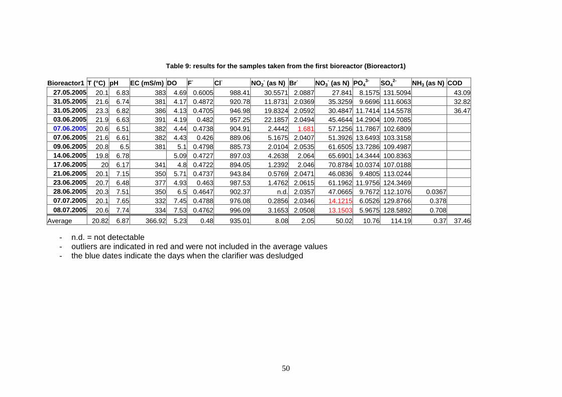
50

Table 9: results for the samples taken from the first bioreactor (Bioreactor1)

Bioreactor1 T (°C) pH EC (mS/m) DO F-

Cl-

NO2

- (as N) Br

-NO3

- (as N) PO4

3-SO4

2-NH3 (as N) COD

27.05.2005 20.1 6.83 383 4.69 0.6005 988.41 30.5571 2.0887 27.841 8.1575 131.5094 43.09

31.05.2005 21.6 6.74 381 4.17 0.4872 920.78 11.8731 2.0369 35.3259 9.6696 111.6063 32.82

31.05.2005 23.3 6.82 386 4.13 0.4705 946.98 19.8324 2.0592 30.4847 11.7414 114.5578 36.47

03.06.2005 21.9 6.63 391 4.19 0.482 957.25 22.1857 2.0494 45.4644 14.2904 109.7085

07.06.2005 20.6 6.51 382 4.44 0.4738 904.91 2.4442 1.681 57.1256 11.7867 102.6809

07.06.2005 21.6 6.61 382 4.43 0.426 889.06 5.1675 2.0407 51.3926 13.6493 103.3158

09.06.2005 20.8 6.5 381 5.1 0.4798 885.73 2.0104 2.0535 61.6505 13.7286 109.4987

14.06.2005 19.8 6.78 5.09 0.4727 897.03 4.2638 2.064 65.6901 14.3444 100.8363

17.06.2005 20 6.17 341 4.8 0.4722 894.05 1.2392 2.046 70.8784 10.0374 107.0188

21.06.2005 20.1 7.15 350 5.71 0.4737 943.84 0.5769 2.0471 46.0836 9.4805 113.0244

23.06.2005 20.7 6.48 377 4.93 0.463 987.53 1.4762 2.0615 61.1962 11.9756 124.3469

28.06.2005 20.3 7.51 350 6.5 0.4647 902.37 n.d. 2.0357 47.0665 9.7672 112.1076 0.0367

07.07.2005 20.1 7.65 332 7.45 0.4788 976.08 0.2856 2.0346 14.1215 6.0526 129.8766 0.378

08.07.2005 20.6 7.74 334 7.53 0.4762 996.09 3.1653 2.0508 13.1503 5.9675 128.5892 0.708

Average 20.82 6.87 366.92 5.23 0.48 935.01 8.08 2.05 50.02 10.76 114.19 0.37 37.46

- n.d. = not detectable

- outliers are indicated in red and were not included in the average values

- the blue dates indicate the days when the clarifier was desludged

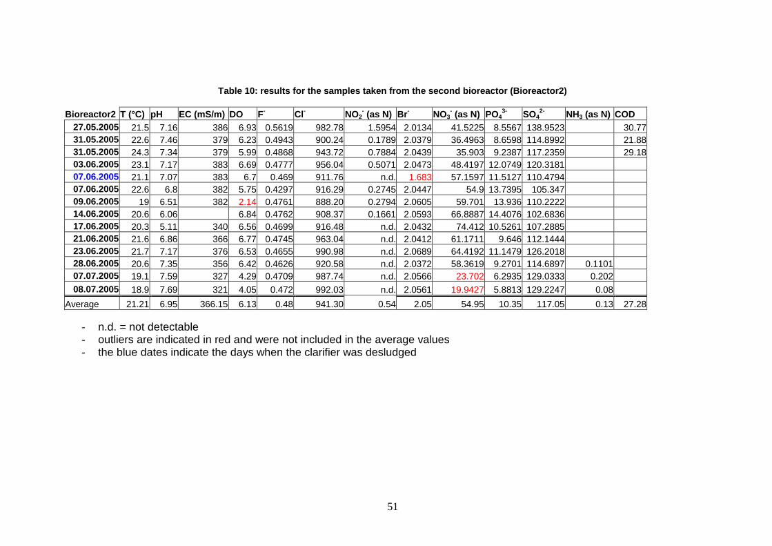
51

Table 10: results for the samples taken from the second bioreactor (Bioreactor2)

Bioreactor2 T (°C) pH EC (mS/m) DO F-

Cl-

NO2

- (as N) Br

-NO3

- (as N) PO4

3-SO4

2-NH3 (as N) COD

27.05.2005 21.5 7.16 386 6.93 0.5619 982.78 1.5954 2.0134 41.5225 8.5567 138.9523 30.77

31.05.2005 22.6 7.46 379 6.23 0.4943 900.24 0.1789 2.0379 36.4963 8.6598 114.8992 21.88

31.05.2005 24.3 7.34 379 5.99 0.4868 943.72 0.7884 2.0439 35.903 9.2387 117.2359 29.18

03.06.2005 23.1 7.17 383 6.69 0.4777 956.04 0.5071 2.0473 48.4197 12.0749 120.3181

07.06.2005 21.1 7.07 383 6.7 0.469 911.76 n.d. 1.683 57.1597 11.5127 110.4794

07.06.2005 22.6 6.8 382 5.75 0.4297 916.29 0.2745 2.0447 54.9 13.7395 105.347

09.06.2005 19 6.51 382 2.14 0.4761 888.20 0.2794 2.0605 59.701 13.936 110.2222

14.06.2005 20.6 6.06 6.84 0.4762 908.37 0.1661 2.0593 66.8887 14.4076 102.6836

17.06.2005 20.3 5.11 340 6.56 0.4699 916.48 n.d. 2.0432 74.412 10.5261 107.2885

21.06.2005 21.6 6.86 366 6.77 0.4745 963.04 n.d. 2.0412 61.1711 9.646 112.1444

23.06.2005 21.7 7.17 376 6.53 0.4655 990.98 n.d. 2.0689 64.4192 11.1479 126.2018

28.06.2005 20.6 7.35 356 6.42 0.4626 920.58 n.d. 2.0372 58.3619 9.2701 114.6897 0.1101

07.07.2005 19.1 7.59 327 4.29 0.4709 987.74 n.d. 2.0566 23.702 6.2935 129.0333 0.202

08.07.2005 18.9 7.69 321 4.05 0.472 992.03 n.d. 2.0561 19.9427 5.8813 129.2247 0.08

Average 21.21 6.95 366.15 6.13 0.48 941.30 0.54 2.05 54.95 10.35 117.05 0.13 27.28

- n.d. = not detectable

- outliers are indicated in red and were not included in the average values

- the blue dates indicate the days when the clarifier was desludged

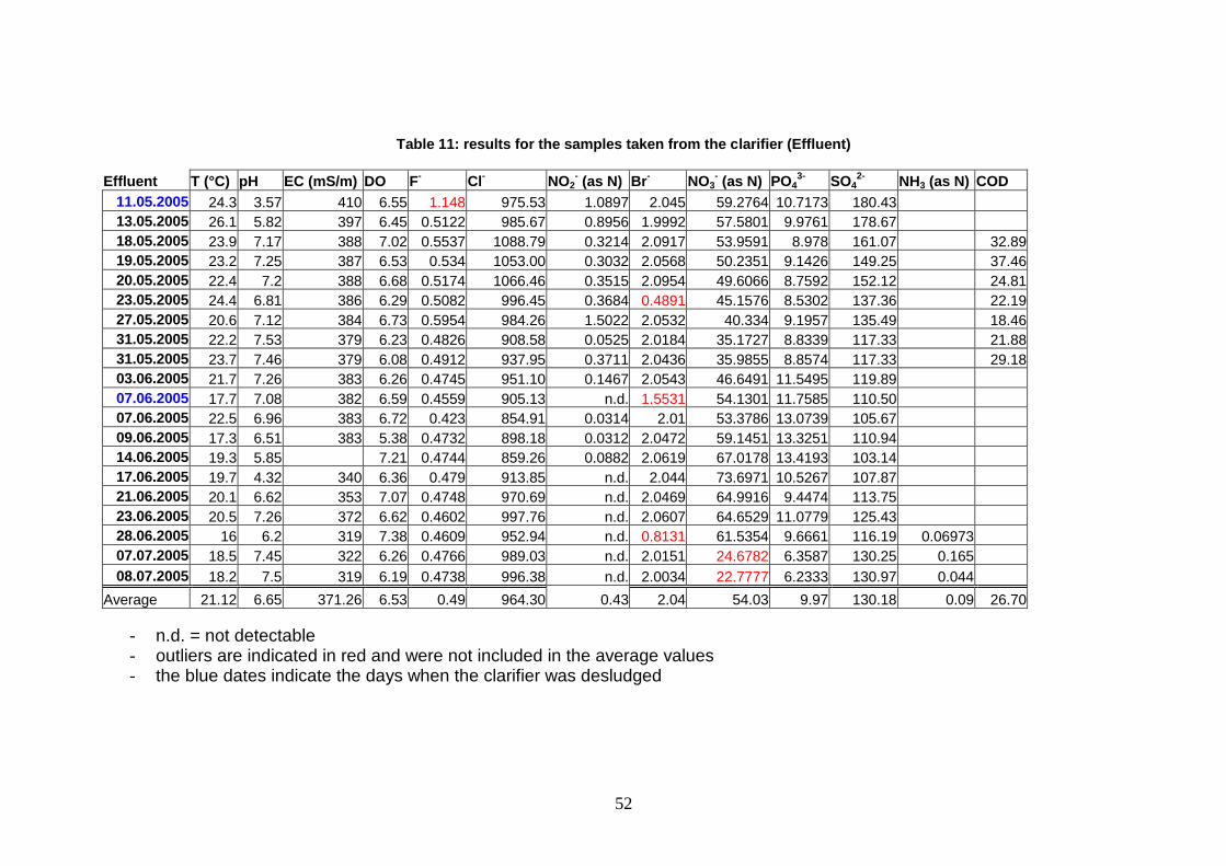
52

Table 11: results for the samples taken from the clarifier (Effluent)

Effluent T (°C) pH EC (mS/m) DO F-

Cl-

NO2

- (as N) Br

-NO3

- (as N) PO4

3-SO4

2-NH3 (as N) COD

11.05.2005 24.3 3.57 410 6.55 1.148 975.53 1.0897 2.045 59.2764 10.7173 180.43

13.05.2005 26.1 5.82 397 6.45 0.5122 985.67 0.8956 1.9992 57.5801 9.9761 178.67

18.05.2005 23.9 7.17 388 7.02 0.5537 1088.79 0.3214 2.0917 53.9591 8.978 161.07 32.89

19.05.2005 23.2 7.25 387 6.53 0.534 1053.00 0.3032 2.0568 50.2351 9.1426 149.25 37.46

20.05.2005 22.4 7.2 388 6.68 0.5174 1066.46 0.3515 2.0954 49.6066 8.7592 152.12 24.81

23.05.2005 24.4 6.81 386 6.29 0.5082 996.45 0.3684 0.4891 45.1576 8.5302 137.36 22.19

27.05.2005 20.6 7.12 384 6.73 0.5954 984.26 1.5022 2.0532 40.334 9.1957 135.49 18.46

31.05.2005 22.2 7.53 379 6.23 0.4826 908.58 0.0525 2.0184 35.1727 8.8339 117.33 21.88

31.05.2005 23.7 7.46 379 6.08 0.4912 937.95 0.3711 2.0436 35.9855 8.8574 117.33 29.18

03.06.2005 21.7 7.26 383 6.26 0.4745 951.10 0.1467 2.0543 46.6491 11.5495 119.89

07.06.2005 17.7 7.08 382 6.59 0.4559 905.13 n.d. 1.5531 54.1301 11.7585 110.50

07.06.2005 22.5 6.96 383 6.72 0.423 854.91 0.0314 2.01 53.3786 13.0739 105.67

09.06.2005 17.3 6.51 383 5.38 0.4732 898.18 0.0312 2.0472 59.1451 13.3251 110.94

14.06.2005 19.3 5.85 7.21 0.4744 859.26 0.0882 2.0619 67.0178 13.4193 103.14

17.06.2005 19.7 4.32 340 6.36 0.479 913.85 n.d. 2.044 73.6971 10.5267 107.87

21.06.2005 20.1 6.62 353 7.07 0.4748 970.69 n.d. 2.0469 64.9916 9.4474 113.75

23.06.2005 20.5 7.26 372 6.62 0.4602 997.76 n.d. 2.0607 64.6529 11.0779 125.43

28.06.2005 16 6.2 319 7.38 0.4609 952.94 n.d. 0.8131 61.5354 9.6661 116.19 0.06973

07.07.2005 18.5 7.45 322 6.26 0.4766 989.03 n.d. 2.0151 24.6782 6.3587 130.25 0.165

08.07.2005 18.2 7.5 319 6.19 0.4738 996.38 n.d. 2.0034 22.7777 6.2333 130.97 0.044

Average 21.12 6.65 371.26 6.53 0.49 964.30 0.43 2.04 54.03 9.97 130.18 0.09 26.70

- n.d. = not detectable

- outliers are indicated in red and were not included in the average values

- the blue dates indicate the days when the clarifier was desludged