UNIVERSITI PUTRA MALAYSIA

THE EFFECT OF REPARAMETERISATION ON THE BEHAVIOUR OF NONLINEAR ESTIMATES

NORAZAN BINTI MOHAMED RAMLI

FSAS 2000 4

THE EFFECT OF REPARAMETERISATION ON THE BEHAVIOUR OF NONLINEAR ESTIMATES

By

NORAZAN BINTI MOHAMED RAMLI

Thesis Submitted in Fulfilment of the Requirements for the Degree of Master of Science in thE� Faculty of

Science and Environmental Studies Universiti Putra Malaysia

May 2000

TO MY HUSBAN D

2

Abstract of thesis presented to the Senate of Universiti Putra Malaysia in fulf ilmen t of the requirements for the degree of Master of Science.

THE EFFECT OF REPARAMETERISATION ON THE BEHAVIOUR OF NONLINEAR ESTIMATES

By

NORAZAN BINTI MOHAMED RAMLI

May 2000

Chairman: Habshah Bt. Midi, Ph.D.

Faculty: Science and Environmental Studies

This thesis discussed nonlinear modeling and measures o f nonlinear

behaviour. A set of data, representing the average weight o f dried to bacco

leaves (in gra ms) per tree against the ti me in week, was used in this research .

Several nonlinear models were used to fit the data, ho wever only the

Go mpert z and the Logistic models were found to be suita ble . The esti mates o f

the para meters were calculated by using the Gauss-Ne wton algorith m in S-

PLUS Progra mming Language .

A good estimator was the one which had the proper ties closed to the

behaviour o f a linear esti mate . The non linear behaviour o f the esti mates was

assessed using two different approaches , na mely the analytical and the

e mpirical approaches . These approaches were e mployed so that they could

co mple ment the existence of any laggings .

3

The stu dy sho we d that the analytical approach of curvature measures of Bates

an d Watts coul d measure the avera ge nonlinearity but coul d not determine the

parameters that cause d the nonlinear behaviour. Mean while, the bias formula

of Box coul d only give the percenta ge of the extent to which the parameter

estimates may excee d or fall short of the true parameter value, but coul d not

be use d to compare different parameteri zations.

An a dvanta ge of usin g direct measure of s ke wness of Hougaar d was that it

was scale -in depen dent an d coul d be use d to measure nonlinearity in di fferent

parameteri zations. The empirical approach of simulation studies ha d

successfully reveale d the full extent of the nonlinear behaviour of the

estimates an d at the same time , su ggeste d useful reparameteri zations.

Reparameteri zation was use d in or der to remove or re duce the nonlinear

behaviour of the parameter estimates . The study sho we d that the nonlinear

behaviour of the parameter estimates was successfully re duce d after

reparameteri zation. The Lo gistic mo del in a reparameteri ze d mo del function

was foun d to best fit the data as it has the lo west nonlinear measures an d

therefore the closest-to-linear behaviour.

4

Abstrak tesis yang dikemukakan kepada Senat Unive rsiti Putra Ma laysia se bagai memenuhi keper luan untu k ija zah Master Sains .

KESAN PEMPARAMETERAN SEMULA KE ATAS TINGKAHLAKU PENGANGGAR TAKLINEAR

O leh

NORAZAN BINTI MOHAMED RAMLI

Mei 2000

Pengerusi: Habshah Bt Midi, Ph.D.

Fakulti: Sains dan Pengajian Alam Sekitar

T esis ini mem bincang kan pe rmode lan ta klinear dan su katan ting kah la ku

ta klinear. Satu set data yang me wa ki li purata berat daun tem ba kau kering

sepo ko k (da lam gram) mengi kut masa da lam minggu, diguna kan da lam

penye lidi kan ini. 8e berapa mode l ta klinear diguna kan untu k memode l kan

data , wa lau bagaimanapun hanya mode l Gompert z dan mode l Logistic sahaja

yang didapati sesuai. Ni lai-ni lai penganggar di kira mengguna kan pende katan

Gauss - Ne wton dalam bahasa komputer S-PLU S.

Penganggar yang bai k ia lah penganggar yang ting kahla kunya hampir sama

dengan penganggar linear. Ting kah la ku ta klinear dini lai mengguna kan dua

pende katan yang ber beza iaitu secara ana liti k dan empiri k . Pende katan yang

5

berbeza digunakan supaya dapat mengimbangi sebarang kekurangan yang

wujud .

Kaj ian mendapati pendekatan anal itik sukatan kelencongan Bates dan Watts

dapat mengukur tahap sifat taklinear secara purata , tetapi tidak dapat

menentukan parameter yang menyebabkan wujudnya tingkahlaku takl inear

dalam model . Rumus pincang oleh Box pula hanya dapat memberi peratusan

sejauh mana sesuatu penganggar kurang atau lebih daripada n i la i yang

sepatutnya tetapi tidak dapat digunakan sebagai pengukur takl inear untuk

perbandingan dua pemparameteran yang berbeza .

Kelebihan yang ada menggunakan ukuran kepencongan oleh Hougaard ia lah

ianya adalah bebas skala dan boleh digunakan untuk meni la i t ingkah laku

takl inear dalam pemparameteran yang berbeza untuk d ibuat satu

perband ingan. Pendekatan empirik dalam kaedah simu lasi pula dapat

mendedahkan sejauh mana tingkahlaku takl inear penganggar dan pada

masa yang sama mencadangkan pemparameteran semula yang berguna.

Pemparameteran semula digunakan untuk mengu rangkan atau membuang

tingkahlaku takl inear penganggar. Kaj ian menunjukkan tingkah laku takl inear

penganggar dapat d ikurangkan dengan jayanya selepas proses

pemparameteran semula . Model Logistic dalam fungsi model yang

diparameterkan semula telah dipi l ih sebagai model yang lebih baik untuk

6

memodelkan data yang diberi kerana model ini mempunyai tingkahlaku

taklinear yang terkecil dalam sUkatan kelencongan penganggarnya dan

dengan itu yang pa ling hampir dengan ting ka hla ku linear.

7

ACKNOWLEDGEMENTS

F irst and foremost, praise be to God for giving me the strength and patience to

complete th is work. Gratefu l ly, I wou ld l ike to thank my su pervisor Dr .

Habshah Mid i for her excel lent su pervision , invaluable gu idance , helpfu l

d iscussions and continous encou ragement, without which this work would not

be fin ished. My thanks must also extend to the members of my sup�rvisor

committee, Associate Professor D r. Mu hammad Idreess Ahmad and D r.

Kassim Haron for their invaluable d iscussions, comments and help . S imi lar

thanks should go to Pejabat MARDI , Serdang for providing me the sample

data set needed for this study.

8

I certify that an Examination Committee met on 5th

May 2000 to conduct the final examination of Norazan Binti Mohamed Ramli on her Master thesis entitled "The Effect of Reparameterisation on the Behaviour of Nonl inear Estimates" i n accordance with Universiti Pertanian Malaysia (H igher Degree) Act 1980 and U niversiti Pertan ian Malaysia (H igher Degree) Regulations 1981. The committee recommends that the candidate be awarded the relevant degree. Members of the Examination Committee are as fol lows:

Isa Bin Daud, Ph .D . Associate Professor Faculty of Science and Environmental Studies Universiti Putra Ma laysia (Chairman)

Habshah Midi, Ph .D . Faculty of Science and Environmental Stud ies Universiti Putra Malaysia (Member)

Muhammad Idreess Ahmad, Ph .D . Associate Professor Faculty of Science and Environmental Stud ies Universiti Putra Malaysia (Member)

Kassim Haron, Ph .D . Faculty of Science and Environmental Studies Un iversiti Putra Malaysia (Member)

. G HAZALI MOHAY ID I N, Ph .D . Professor/Deputy Dean of Graduate School, Universiti Putra Malaysia

Date: r12 MAY 2000

9

This thesis submitted to the Senate of Universiti Putra Malaysia and was accepted as fulfilment of the requirements for the degree of Master of Science.

10

KAMIS AWANG, Ph . D . Associate Professor, Dean of Graduate School, Universiti Putra Malaysia

Date: ,1 3 JUl 2000.

DECLARATION

hereby declare that the thesis is based on my original work except for quotations and citations wh ich have been du ly acknowledged . I a lso declare that it has not been previously or concurrently submitted for any degree at UPM or other institutions.

Date: 10. b' � 0"00

11

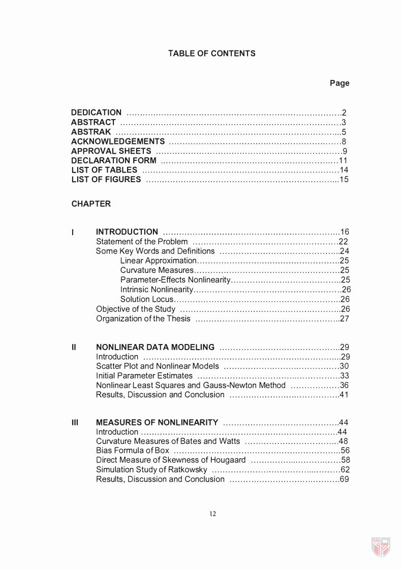
TABLE OF CONTENTS

Page

DEDICATION . . . . . . . . . . . . . . . . . . . . . . . . . . . . . . . . . . . . . . . . . . . . . . . . . . . . . . . . . . . . . . . . . . . . . . . . . . . . . . . . 2 ABSTRACT . . . . . . . . . . . .. . . . . . . . . . . . . . . . . . . . . . . . . . . . . . . . . . . . . . . . . . . . . . . . . . . . . . . . . . . . . . . . . . . . . . 3 ABSTRAK . . . . . . . . . . . . . . . . . . . . . . . . . . . . . . . . . . . . . . . . . . . . . . . . . . . . . . . . . . . . . . . . . . . . . . . . . . . . . . . . . . . . 5 ACKNOWLEDGEMENTS . . . . . . . . . . . . . . . . . . . . . . . . . . . .. . . . . . . . . . . . . . . . . . . . . . . . . . . . . . . . . . . . 8 APPROVAL SHEETS . . . . . . . . . . .. . . . . . . . . . . . . . . . . . . . . . . . . . . . . . . . . . . . . . . . . . . . . . . . . . . . . . . . . . 9 DECLARATION FORM . . . . . . . . . . . . . . . . . . . . . . . . . . . . . . . . . . . . .. . . . . . . . . . . . . . . . . . . . . . . . . . . . . 1 1 LIST OF TABLES ......................................................................... 1 4 LIST OF FIGURES . . . . . . . . . . . . . . . . . . . . . . . . . . . . . . . . . .. . . . . . . . . . . . . . . . . . .. . . . . . . . . . . . . . . . . . . 1 5

CHAPTER

INTRODUCTION .................................................................. 1 6 Statement of the Problem . . . . . . . . . . . . . . . . . . . . . . . .. . . . . . . . . . . . . . . . . . . . . . . . . . . . . . 22 Some Key Words and Defin itions . . . . . . . . . . . . . . . . . . . . . . . . . . . . . . . . . . . . . . . . . . . . . 24

Linear Approximation . . . . . . . . . . . . . . . . . . . . . . . . . . . . . . . . . . . . . . . . . . . . . . . . . . . . . 25 Curvature Measures . . . . . . . . . . . . . . . . . . . . . . . . . . . . . . . . . . . . . . . . . . . . . . . . . . . . . . 25 Parameter-Effects Nonl inearity . . . . . . . . . . . . . . . . . . . . . . . . . . . . . . . . . . . . . . . . . 25 I ntrinsic Nonl inearity . . . . . . . . . . . . . . . . . . . . . . . . . . . . . . . . . . . . . . . . . . . . . . . . . . . . . . . 26 Solution Locus . . . . . . . . . . . . . . . . . . . . . . . . . . . . . . . . . . . . . . . . . . . . . . . . . . . . . . . . . . . . . . 26

Objective of the Study . . . . . . . . . . . . . . . . . .. . . . . . . . . . . . . . . . . . . . . . . . . . . . . . . . . . . . . . . . . . 26 Organization of the Thesis . . . . . . . . . . . . . . . . . . . . . . . . . . . . . . . . . . . . . . . . . . . . . . . . . . . . . . 27

II NONLIN EAR DATA MODELING . . . . . . . . . . . . . . . . . . . . . . . . . . . . . . . . . . . . . . . . . . . . . 29 I ntroduction . . . . . . . . . . . . . . . . . . .. . . . . . . . . . . . . . . . . . . . . . . . . . . . . . . . . . . . . . . . . .. . . . . . . . . . . . . 29 Scatter Plot and Nonl inear Models . . . . . . . . . . . . . . . . . . . . . . . . . . . . . . . . . . . . . . . . . . . 30 I n itial Parameter Estimates . . . . . . . . . . .. . . . . . . . . . . . . . . . . . . . . . . . . . . . . . . . . . . . . . . . . . 33 Non l inear Least Squares and Gauss-Newton Method . . . . . . . . . . . . . . . . . . 36 Results, Discussion and Conclusion . . . . . . . . . . . . . . . . . . . . . . . . . . . . . . . . . . . . . . . . .4 1

III M EASURES OF NONLIN EARITY . . . . . . . . . . . . . . . . . . . . . . . . . . . . . . . . . . . . . . . . . . .44 I ntroduction . . ... . . . . .. . . . . . . . . . . . . . . . . . . . . . . . . . . . . . . . . . . . .. . . . . . . . . . . . . . . . . . . . . . . . . . 44 Curvature Measures of Bates and Watts . . . . . . . . . . . . . . . . . . . . . . . . . . . . . . . . . . .48 Bias Formula of Box . . . . . . . . . . . . . . . . . . . . . . . . . . . . . . . . . . . . . . . . . . . . . . . . . . . . . . . . . . . . . . 56 D irect Measure of Skewness of Hougaard . . . . . . . . . . . . . . . . . . . . . . . . . . . . . . . . . . 58 Simu lation Study of Ratkowsky . . . . . . . . . . . . . . . . . . . . . . . . . . . . . . . . . . . . . . . . . . . . . . . . 62 Results , D iscussion and Conclusion . . . . . . . . . . . . . . . . . . . . . . . . . . . . . . . . . . . . . . . . . 69

12

IV REPARAMETERISATION . . . . . . . . . . . . . . . . . . . . . . . . . . . . . . . . . . . . . . . . . . . . . . . . . . . . 73 I ntroduction . . . . . . . . . . . . . . . . . . . . . . . . . . . . . . . . . . . . . . . . . . . . . . . . . . . . . . . . . . . . . . . . . . . . . . . . 73 Some Gu idel ines on Reparameterisations . . . . . . . . . . . . . . . . . . . . . . . . . . . . . . . . . 74 Su i table Reparameterisations for Gompertz and Logistic Models . . . . 78 Resu lts , D iscussions and Conclus ion . . . . . . . . . . . . . . . . . . . . . . . . . . . . . . . . . . . . . . . 85

V CONCLUSION AND SUGGESTION FOR FURTHER RESEARCH . . 87 Conclusions . . . . . . . . . . . . . . . . . . . . . . . . . . . . . . . . . . . . . . . . . . . . . . . . . . . . . . . . . . . . . . . . . . . . . . . . . 87

B IBLIOGRAPHY . . . . . . . . . . . . . . . . . . . . . . . . . . . . . . . . . . . . . . . . . . . . . . . . . . . . . . . . . . . . . . . . . . . 93

APPENDICES . . . . . . . . . . . . . . . . . . . . . . . . . . . . . . . . . . . . . . . . . . . . . . . . . . . . . . . . . . . . . . . . . . . . . . 96 Append ix A - Computer Programs used to calcu late values needed in Chapter I I . . . . . . . . . . . . . . . . . . . . . . . . . . . . . . . . . . . . . . . . . . . . . . . . . . . . . . 97 Appendix B - Computer Programs used to calcu late values needed in Chapter I I I and IV . . . . . . . . . . . . . . . . . . . . . . . . . . . . . . . . . . . . . . . . . . 1 03

VITA . . . . . . . . . . . . . . . . . . . . . . . . . . . . . . . . . . . . . . . . . . . . . . . . . . . . . . . . . . . . . . . . . . . . . . . . . . . . . . . . . . . 1 25

13

Table

1

2

3

4

5

6

7

8

9

1 0

1 1

1 2

1 3

1 4

1 5

1 6

17

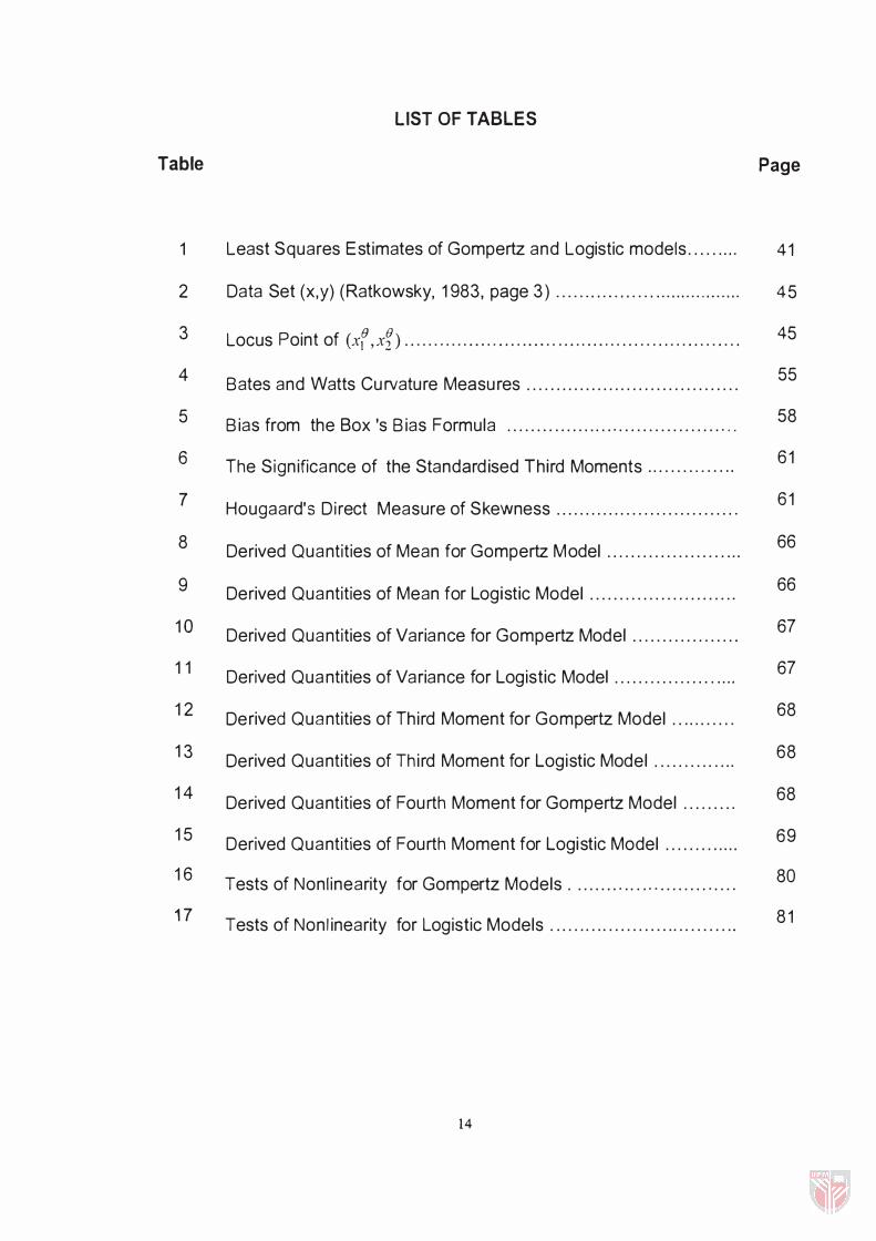
LIST OF TABLES

Least Squares Estimates of Gompertz and Logistic models . . . . . . . . .

Data Set (x,Y) (Ratkowsky, 1 983, page 3 ) . . . . . . . . . . . . . . . . . . . . . . . . . . . . . . . . . .

Locus Point of (xf ,xf ) . . . . . . . . . . . . . . . . . . . . . . . . . . . . . . . . . . . . . . . . . . . . . . . . . . . . . . . . .

Bates and Watts Curvature Measu res . . . . . . . . . . . . . . . . . . . . . . . . . . . . . . . . . . . .

Bias from the Box 's Bias Formula . . . . . . . . . . . . . . . . . . . . . . . . . . . . . . . . . . . . . . .

The Sign ificance of the Standard ised Third Moments . . . . . . . . .. . . . . .

Hougaard's Di rect Measure of Skewness . . . . . . . . . . . . . . . . . . . . . . . . . . . . . . .

Derived Quantities of Mean for Gompertz Model . . . . . . . . . . . . . . . . . . . . . . .

Derived Quantities of Mean for Logistic Model . . . . . . . . . . . . . . . . . . . . . . . . .

Derived Quantities of Variance for Gompertz Model . . . . . . . . . . . . . . . . . .

Derived Quantities of Variance for Logistic Model . . . . . . . . . . . . . . . . . . . . .

Derived Quantities of Th ird Moment for Gompertz Model . . . . . . . . . . .

Derived Quantities of Th i rd Moment for Logistic Model . . . . . . . . . . . . . .

Derived Quantities of Fourth Moment for Gompertz Model . . . . . . . . .

Derived Quantities of Fourth Moment for Logistic Model . . . . . . . . . . . . .

Tests of Nonl inearity for Gompertz Models . . . . . . . . . . . . . .. . . . . . . . . . . . . .

Tests of Nonlinearity for Logistic Models . . . . . . . . . . . . . . . . . . . . . . . . . . . . . . . .

14

Page

41

45

45

55

58

6 1

6 1

66

66

67

67

68

68

68

69

80

8 1

Figure

1

2

3

4

5

6

7

8

9

1 0

1 1

1 2

1 3

1 4

1 5

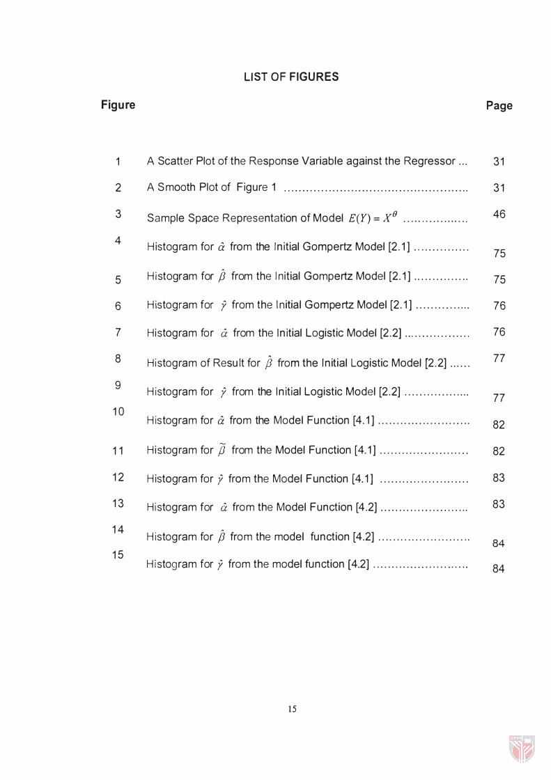
LIST OF FIGURES

A Scatter Plot of the Response Variable against the Regressor . . .

A S mooth Plot of Figure 1 . . . . . . . . . . . . . . . . . . . . . . . . . . . . . . . . . . . . . . . . . . . . . . . . . .

Sample Space Representation of Model E(Y) = XB ................. .

H istogram for eX from the I n itial Gompertz Model [2 . 1 ] . . . . . . . . . . . . . . .

H i stogram for jJ from the In itial Gompertz Model [2 . 1 ] . . . . . . . . . . . . . . .

Histogram for y from the In it ia l Gompertz Model [2 . 1 ] . . . . . . . . . . . . . . .

Histogram for eX from the I n itial Logistic Model [2 .2] . .. . . . . . . . . . . . . . . .

Histogram of Resu lt for jJ from the I n it ial Logistic Model [2 .2] . . . . . .

H istogram for y from the I n itial Logistic Model [2 .2] . . . . . . . . . . . . . . . . . .

H istogram for eX from the Model Function [4. 1 ] . . . . . . . . . . . . . . . . . . . . . . . . .

Histogram for jJ from the Model Function [4. 1 ] . . . . . . . . . . . . . . . . . . . . . . . .

H istogram for y from the Model Function [4. 1 ] . . . . . . . . . . . . . . . . . . . . . . . .

Histogram for eX from the Model Function [4 .2] . . . . . . . . . . . . . . . . . . . . . . . .

H istogram for jJ from the model function [4.2] . . .. . . . . .... . . . . . . . . . .. . .

H i stogram for y from the model function [4.2] . . . . . . . . . . . . . . . . . . . . . . . . . .

15

Page

31

3 1

46

75

75

76

76

77

77

82

82

83

83

84

84

CHAPTER 1

I NTRODUCTION

One of the important tasks in statistics is to find the relationships, if any, that

exist in a set of variables. I n data model ing, one of the variables, often being

cal led the response or dependent variable is denoted by y. This variable

normal ly becomes our particular i nterest. The other variable , which we

normal ly cal l explanatory variable or independent variable or regressor, is to

expla in the behaviour of y, and is denoted by x.

I n order to have a rough idea of some relationship between y and x, we

normally do a scatter plot of y against x whereby we can express this

relationship via some function x and mathematical ly we can write it as

where 8 = (81) 82, ... ,8 p)T is a set of p unknown parameters and Et is an

add itive error term. If the errors 5t (t= 1 ,2 , . . . , n ) satisfy E ( Et )=0 and

Var( E t )= 0'2, then the value {j which min imises the sum of squares of

residuals

n

S(8) = 2:)Yt -I(Xt, 8)]2 [ 1 . 2] t=1

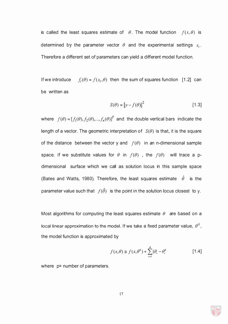
is cal led the least squares estimate of e. The model function I(x, e) is

determined by the parameter vector e and the experimental sett ings XI'

Therefore a d ifferent set of parameters can yield a d ifferent model function .

If we introduce !tee) = I(xt,e) then the sum of squares function [ 1 . 2] can

be written as

See) = lIy - l(e)112 [ 1 .3]

where I(e) = [jj(e),f2(e), ... ,fn(e)]T and the double vertical bars ind icate the

length of a vector. The geometric interpretation of See) is that, it is the square

of the d istance between the vector y and I(e) i n an n-d imensional sample

space. If we substitute values for e i n I(e) , the I(e) wil l trace a p-

dimensional surface which we call as solution locus in this sample space

(Bates and Watts, 1 980). Therefore, the least squares estimate B is the

parameter value such that feB) is the point i n the solution locus closest to y.

Most algorithms for computing the least squares estimate e are based on a

local linear approximation to the model. If we take a f ixed parameter value, eO,

the model function is approximated by

where p= number of parameters.

p

f(x,e) == f(x,eo) + 2)e, - B,o )v, [ 1 .4] ,=1

17

Equivalently , [1 .4] can be written as

p feB) == I(Bo) + LCBl - B1o)v1 [ 1 . 5J

where

1=1

oICx,B) ( i=1 ,2 , . . . , p ) is evaluated at oB,

When us ing l inear approximation, we are to replace the solution locus by it

tangent plane at ICBo) , and at the same time to impose a un iform co-ordinate

system on that tangent p lane. Bates and Watts ( 1 980 & 1 988) termed these

two components of the l inear approximation as the planar assumption and the

un iform co-ordinate assumption respectively.

The measures, which ind icate the adequacy of a l inear approximation , are

called the measures of the nonl inearity. The very first attempt to measure

nonl inearity was made by Beale in 1 960 (Ratkowsky, 1 983) . Box a lso

presented a formula for estimating the bias in the least square estimators

which is known as the Box bias formula (Cook, 1 986). Ratkowsky ( 1 983) used

s imulation studies not only to predict bias to the correct order of magnitude but

a lso to the correct extent of nonl inear behaviour of the model . Bates and Watts

also developed new measu res of nonl inearity but it was based on the

geometric concept of curvature (Bates and Watts, 1 980). To determine how

planar the expectation surface is and how un iform the parameter l ines are on

18

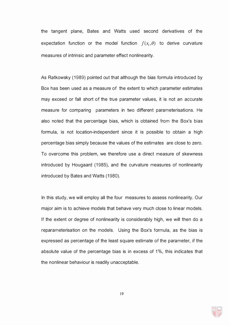
the tangent plane, Bates and Watts used second derivat ives of the

expectat ion function or the model function f(xt,B) to derive curvature

measu res of int rins ic and parameter effect nonl inearity.

As Ratkowsky ( 1 989) pointed out that although the bias formula int roduced by

Box has been used as a measu re of the extent to wh ich parameter est imates

may exceed or fal l short of the true parameter values, it is not an accurate

measu re for comparing parameters in two d ifferent parameterisat ions. He

also noted that the percentage bias, which is obta ined f rom the Box's b ias

formula , is not locat ion-independent s ince it is possible to obta in a h igh

percentage bias s imply because the values of the est imates are close to zero.

To overcome th is problem, we therefore use a d irect measure of skewness

int roduced by Hougaard ( 1 985), and the curvature measu res of nonl inearity

int roduced by Bates and Watts ( 1 980).

In th is study, we wil l employ al l the four measu res to assess nonl inearity. Our

major aim is to achieve models that behave very much close to l inear models.

If the extent or degree of nonl inearity is considerably h igh, we wil l t hen do a

reparameterisat ion on the models. Using the Box's formula , as the bias is

expressed as percentage of the least square est imate of the parameter, if t he

absolute value of the percentage bias is in excess of 1 %, th is ind icates that

the nonl inear behaviour is read ily unacceptable.

19

The stat ist ical s ign ificance o f int rins ic and pa ram et er eff ect nonl in earity o f

Bates and Watts may be assessed by comparing these values with l-F

where F = F (p, n-p, a) is o bta ined from the F -distri but ion ta ble

corresponding to signi ficance level a. The solution locus may be considered

to be su fficiently linear over an approximate 95% con fidence region if intrinsic

nonl inearity is less than l-F. Sim ilarly, the projected parameter lines o f ()

may be assumed to be su fficiently paralle l and uni form ly spaced if the

parameter e ffect is less than l-F.

One o f the advantages o f using s imulation studies is that we can study the

sampl ing propert ies o f the least square est imators. Using the parameter

est imates o bta ined from the s imulat ion studies, we w ill calculate the f irst fou r

moments o f the set o f est imates, namely, the sample mean ml' the sample

var iance mz, the s ke wness coe ffic ient gl = m� , and the kurtosis coeffic ient

H mZ 2

m gz = (--T) - 3 where m3 and m4 are the th ird and t he fourt h sample moments

mz

a bout the mean respect ive ly. Based on the a bove four moments, we then

exam ine whether the est imator exh ib its norma l behav iour by per forming a

standard-normal d istri but ion test on the moments sa id earlier .

20

The closeness of the set of simulated parameter estimates approaching to a

normal distribution can also be visually assessed by examining the histogram

of each parameter. In fact, the histogram will clearly illustrate whether the least

square estimators having a negative or positive skewness .

To calculate the Hougaard d irect measure of skewness, we need to find the

estimate of the third moment of each parameter and standard ise it using the

appropriate element of asymptotic covariance matrix. As there is a close link

between the extent of nonlinear behaviour of an estimator and the extent of

nonnormality in the sampling distribution of the estimator, the standard ised

third moment is then used as a guide whether the estimator is close-to-linear

or contains some considerable nonlinearity. If the standard ised third moment

of the parameter is less than 0.1, then the estimator of the parameter is said to

be very close-to-linear behaviour. If it is in between 0 . 1 and 0 .25 , then the

estimator is reasonably close-to-linear. However if the standard ised third

moment is greater than 0 .25, the skewness is already very apparent.

Therefore, for any standard ised third moments exceeding a value of 1 , this

ind icates that the nonlinear behaviour is already unacceptable.

As we noted, some of these measures of nonlinearity do not identify the

nonlinear-behaving parameters, nor do they suggest su itable

reparameterisations, hence we would rely on the histograms of the parameter

estimates obtained from our simulation studies. As suggested by Ratkowsky

21

(1983), a histogram with a long right�hand tail characterise a lognormal

distribution, so to reparameterise the model, he suggested a replacement of

the parameter in the model function by the exponential of the parameter. On

the other hand, a histogram with a long left�hand tail suggests a replacement

of the parameter by a logarithm of the parameter. A comparison of the various

measures of the nonlinearity for each parameter estimate before and after the

reparameterisation, will reveal whether the reparameterisation really do

improve the nonlinear models to behave closer to linear models.

Statement of the Problem

Nonlinear models are defined as models having at least one parameter

appears nonlinearly, whereby at least one of their derivatives with respect to

any parameters are not independent of their parameters. In the estimation

properties of these models, nonlinear models differ greatly if compared to

linear models. In linear models, with the assumption that the errors are

independent, and identically distributed (LLd), they will result to having

unbiased; normally distributed, and minimum variance estimators. However,

nonlinear models only tend to do so as the sample sizes become very large.

In this study of nonlinear modeling, a set of experimental data representing the

average weight (in grams) of dried tobacco leaves per tree against the time in

week was obtained from MARDI, Serdang. The sample size of this set of data

22

is simi lar to those actual ly obtained in practice by scientists in agricultural

research . So with the given data , we are to fit the data using appropriate

models and fina l ly wil l choose the ones that behave very close to l inear

models .

This research wi l l focus on three aspects of nonlinear modeling. The first is to

estimate the least square estimators of the parameters that exist in the

proposed non l inear models. In order to estimate the parameters of the model,

we will use least square method as mentioned earl ier. Unfortunately, un l ike a

least square estimator of a parameter in linear model , a least square estimator

of a parameter in a nonl inear model has unknown properties for fin ite sample

size. Nevertheless , Ratkowsky (1983) proposed that as sample sizes

increases , we might observe that the estimator wi l l tend to become more and

more unbiased , more and more normal ly distributed and approach a min imu m

possible variance. The solution for approximately minimum variance is

addressed by the use of iterative numerical methods. In this study , we wil l

employ Gauss-Newton method as it is favoured for its fast convergence

characteristic, provided if we have good in it ial parameter estimates or starting

values.

The second part of the study is to measure the nonlinearity in the parameters .

Various widely used methods wil l be incorporated; the Box bias formula , the

Bates and Watts curvature measure, the Ratkowsky simUlation studies and

23

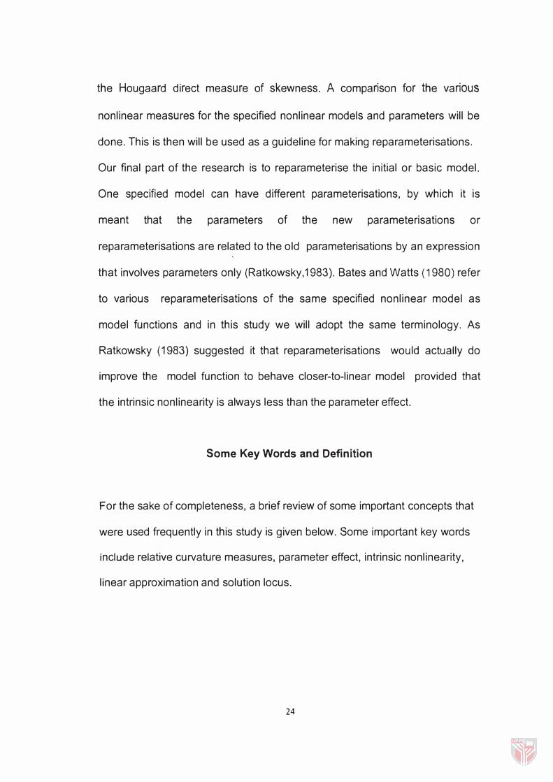
the Hougaard direct measure of skewness. A comparison for the various

nonlinear measures for the specified nonlinear models and parameters will be

done. This is then will be used as a guideline for making reparameterisations.

Our final part of the research is to reparameterise the initial or basic model.

One specified model can have different parameterisations, by which it is

meant that the parameters of the new parameterisations or

reparameterisations are related to the old parameterisations by an expression

that involves parameters only (Ratkowsky,1983). Bates and Watts (1980) refer

to various reparameterisations of the same specified nonlinear model as

model functions and in this study we will adopt the same terminology. As

Ratkowsky (1983) suggested it that reparameterisations would actually do

improve the model function to behave closer-to-linear model provided that

the intrinsic nonlinearity is always less than the parameter effect.

Some Key Words and Definition

For the sake of completeness, a brief review of some important concepts that

were used frequently in this study is given below. Some important key words

include relative curvature measures, parameter effect, intrinsic nonlinearity,

linear approximation and solution locus.

24