
UNIVERSITE DE PARIS XI { U.F.R. DES SCIENCES...
108
UNIVERSITE DE PARIS XI – U.F.R. DES SCIENCES D’ORSAY Habilitation ` a diriger des recherches Sp´ ecialit´ e : Physique Th´ eorique pr´ esent´ ee par Nicolas PAVLOFF Sujet : Physique des agr´ egats m´ etalliques et d´ eveloppements semiclassiques Soutenue le 16 f´ evrier 1999 devant le jury compos´ e de Messieurs Eric AKKERMANS Rapporteur Roger BALIAN Rapporteur Oriol BOHIGAS Pr´ esident Matthias BRACK Rapporteur Philippe CAHUZAC
-
Upload
duongtuyen -
Category
Documents
-
view
219 -
download
0
Transcript of UNIVERSITE DE PARIS XI { U.F.R. DES SCIENCES...

UNIVERSITE DE PARIS XI – U.F.R. DES SCIENCES D’ORSAY
Habilitation a diriger des recherches
Specialite :
Physique Theorique
presentee par
Nicolas PAVLOFF
Sujet :
Physique des agregats metalliques
et developpements semiclassiques
Soutenue le 16 fevrier 1999
devant le jury compose de
Messieurs Eric AKKERMANS RapporteurRoger BALIAN RapporteurOriol BOHIGAS PresidentMatthias BRACK RapporteurPhilippe CAHUZAC


Table des matieres
Avant-propos 5
Liste des publications . . . . . . . . . . . . . . . . . . . . . . . . . . . . . . . . . 6
1 Agregats de metaux simples 9
1.1 Bref survol historique . . . . . . . . . . . . . . . . . . . . . . . . . . . . . . . . . 9
1.2 Le modele de gelee . . . . . . . . . . . . . . . . . . . . . . . . . . . . . . . . . . . 10
1.3 Champ moyen – Effets de couche quantiques . . . . . . . . . . . . . . . . . . . . 12
2 Formule des traces 15
2.1 Un cas unidimensionnel simple . . . . . . . . . . . . . . . . . . . . . . . . . . . . 16
2.2 Systeme a D degres de liberte (D ≥ 2) . . . . . . . . . . . . . . . . . . . . . . . . 16
2.2.1 Methode EBK . . . . . . . . . . . . . . . . . . . . . . . . . . . . . . . . . 16
2.2.2 Formule des traces . . . . . . . . . . . . . . . . . . . . . . . . . . . . . . . 18
2.2.3 Synopsis de la demonstration de la formule des traces . . . . . . . . . . . 19
2.3 Interet pratique de la formule des traces . . . . . . . . . . . . . . . . . . . . . . . 20
2.4 La formule des traces dans la sphere – Supercouches . . . . . . . . . . . . . . . . 22
3 Facettes et diffraction 27
3.1 Agregats metalliques facettes . . . . . . . . . . . . . . . . . . . . . . . . . . . . . 27
3.1.1 Presentation des resultats experimentaux . . . . . . . . . . . . . . . . . . 27
3.1.2 Article : “Shell structure in faceted metal clusters” (ref. [Pav93]) . . . . . 28
3.2 Developpement de Weyl en presence de symetries discretes . . . . . . . . . . . . . 39
3.2.1 Article : “Discrete symmetries in the Weyl expansion for quantum bil-liards” (ref. [Pav94]) . . . . . . . . . . . . . . . . . . . . . . . . . . . . . . 39
3.3 Diffraction . . . . . . . . . . . . . . . . . . . . . . . . . . . . . . . . . . . . . . . . 47
3.3.1 Article : “Diffractive orbits in quantum billiards” (ref. [Pav95b]) . . . . . 48
3.3.2 Approximation uniforme . . . . . . . . . . . . . . . . . . . . . . . . . . . . 53
3.3.3 Article : “Uniform approximation for diffractive contributions to the traceformula in billiard systems” (ref. [Sie97]) . . . . . . . . . . . . . . . . . . . 53
3
4 TABLE DES MATIERES
4 Effets de couche et rugosite 75
4.1 Presentation . . . . . . . . . . . . . . . . . . . . . . . . . . . . . . . . . . . . . . . 75
4.2 Articles . . . . . . . . . . . . . . . . . . . . . . . . . . . . . . . . . . . . . . . . . 78
4.2.1 “Trace formula for an ensemble of bumpy billiards” (ref. [Pav95a]) . . . . 78
4.2.2 “Rough droplet model for spherical metal clusters” (ref. [Pav98]) . . . . . 89
Conclusion et perspectives 101
Bibliographie 103

Avant-propos
Ce memoire a ete redige en vue de l’obtention de l’habilitation a diriger des recherches. Ilfait la synthese des travaux que j’ai effectues depuis 1993 dans les domaines des developpementssemiclassiques et de la physique des agregats metalliques.
Je me suis egalement, au cours de ma these et dans les annees qui ont suivi, interesse a laphysique des systemes inhomogenes d’helium liquide. Cependant, pour preserver la coherencede ce memoire j’ai concentre son contenu sur mes poles d’interets les plus recents et je n’y ai pasinclus de compte-rendu de mes travaux sur l’helium. Ceux-ci sont en grande partie resumes dansma these1 a laquelle je renvoie le lecteur. J’ai egalement fait figurer a la fin de cet avant-proposla liste de mes publications, en marquant celles incluses dans ma these et celles figurant dansce memoire.
J’ai commence a m’interesser a la physique des agregats et aux developpements semiclas-siques en 1991, au cours de mon sejour post-doctoral a l’Institut Niels Bohr de Copenhague. J’aila-bas pu m’initier a la physique des agregats metalliques principalement grace a S. Bjørnholmet B. Mottelson. Ce m’est un grand plaisir de reconnaıtre ici tout ce que je leur dois. Au coursde mon sejour a Copenhague, j’ai egalement cotoye les membres du “chaos group” et j’ai puprofiter de leur dynamisme. C’est en particulier S. Creagh qui m’a interesse aux specificites desdeveloppements en orbites periodiques, approche qui attirait les physiciens des agregats depuislongtemps via le phenomene de supercouche.
A mon retour a Orsay, j’ai continue a m’interesser en parallele a la physique des agregatset aux developpements semiclassiques. J’ai beneficie de l’atmosphere studieuse mais amicale etdetendue qui regne dans le “groupe chaos” que constituent E. Bogomolny, O. Bohigas, M.J.Giannoni, C. Jacquemin, P. Lebœuf, C. Schmit et D. Ullmo pour les membres “permanents”,et S. Creagh, R. Jalabert, A. Mouchet, K. Richter, M. Sieber, N. Whelan . . .pour les membres“temporaires”. C’est un plaisir de tous les remercier pour les nombreuses discussions et inter-actions que j’ai eues avec eux.
Je tiens egalement a remercier E. Akkermans, R. Balian, O. Bohigas, M. Brack et P.Cahuzac d’avoir accepte d’etre membres du jury d’habilitation. En particulier, E. Akkermans,R. Balian et M. Brack ont bien voulu se charger de la tache de rapporteur et je leur en suistres reconnaissant. Merci egalement a M.T. Commault et P. Lebœuf qui ont accepter de relirece manuscrit avec diligeance et efficacitee.
La problematique presentee dans ces pages est double (physique des agregats/methodessemiclassiques). En effet, l’approche semiclassique en physique des agregats metalliques estfructueuse si l’on s’interesse, comme c’est le cas dans ce memoire, a leur structure electronique.Elle permet, dans un cadre theorique simple, une interpretation claire et precise des phenomenesde couche et de supercouche dont les agregats metalliques fournissent le parangon puisqu’on
1Intitulee “Systemes inhomogenes d’helium liquide a temperature nulle”, elle fut soutenue en novembre 1990.5

6 AVANT-PROPOS
a pu observer des couches quantiques dans des agregats contenant jusqu’a 15 000 electrons devalence [Pel95].
Ce memoire debute par un chapitre presentant les grandes lignes de la physique des agregatsde metaux simples et en particulier les approximations permettant de decrire les proprietes destructure electronique. L’outil semiclassique est ensuite presente dans le deuxieme chapitre quidiscute l’interet de l’approche en orbites periodiques d’un point de vue general, puis l’illustreen interpretant le phenomene de supercouche dans la sphere. Dans les deux chapitres suivantson discute de deux aspects specifiques de la physique des agregats : la formation de facettes(chapitre 3 et ref. [Pav93]), et la rugosite de la frontiere (chapitre 4 et ref. [Pav98]). Ces deuxphenomenes sont lies au caractere discret de la structure ionique et sont propres aux agregats.Il est instructif de remarquer qu’ils sont egalement interessants d’un point de vue purementsemiclassique puisqu’ils ont conduit a des developpements theoriques nouveaux : etude descontributions diffractives a la formule des traces [Pav95b, Sie97] ; du developpement de Weylen presence de symetries [Pav94] et de la formule des traces dans un billard a surface aleatoire[Pav95a].
Cet amusant balancier entre les deux poles de ce memoire illustre l’une des lecons quo-tidiennes du “semiclassicien”. Celui-ci observe souvent – a une echelle plus modeste et dansun cadre plus restreint que ne le remarqua initialement H. Poincare – que “la physique nenous donne pas seulement l’occasion de resoudre des problemes . . ., elle nous fait pressentir lasolution”. Du point de vue du physicien des agregats, c’est l’elegance et la simplicite de l’ap-proche semiclassique qui sont remarquables. Outre ses succes dans l’interpretation des effets decouche et de supercouche, on peut remarquer que cette approche permet de traiter simplementet avec precision des problemes dont la solution numerique serait tres lourde (comme celui dela determination du spectre d’un agregat rugueux, cf. refs. [Pav95a, Pav98]).
Enfin, outre l’enrichissement mutuel de deux disciplines que ce memoire espere illustrer, ilfaut souligner le plaisir qu’offre le dialogue entre deux aspects, l’un plus fondamental, l’autreplus concret, de la recherche scientifique.
Liste des publications
Dans la liste qui suit, les publications figurant dans ma these sont marquees par un losangeet celles qui sont incluses dans ce memoire par un trefle.
♦ J. Dupont-Roc, M. Himbert, N. Pavloff et J. Treiner, “Inhomogeous liquid 4He, a densityfunctional approach with a finite range interaction”, J. Low Temp. Physics 81, pp. 31–44(1990).
♦ N. Pavloff et J. Treiner, “3He impurities on liquid 4He : possible existence of excitedstates”, J. Low Temp. Physics 83, pp. 15–39 (1991).
♦ N. Pavloff et J. Treiner, “3He impurity states on liquid 4He, from thin films to the bulksurface”, J. Low Temp. Physics 83, pp. 331–349 (1991).
– F. Dalfovo, J. Dupont-Roc, N. Pavloff, S. Stringari et J. Treiner, “Freezing of superfluidhelium at zero temperature : a density functional approach”, Europhys. Lett. 16, pp.205–210 (1991).
– N. Pavloff et M. S. Hansen, “Effect of surface roughness on the electronic structure ofmetallic clusters”, Z. Phys. D 24, pp. 57–63 (1992).
– E. Bashkin, N. Pavloff et J. Treiner, “Bound states of 3He in 3He–4He mixture films”, J.Low Temp. Physics 99, pp. 659–681 (1995).

AVANT-PROPOS 7
♣ N. Pavloff et S. C. Creagh, “Shell structure in faceted metal clusters”, Phys. Rev. B 48,pp. 18164–18173 (1993).
♣ N. Pavloff, “Discrete symmetries in the Weyl expansion for quantum billiards”, J. Phys.A : Math. Gen. 27, pp. 4317–4323 (1994).
♣ N. Pavloff et C. Schmit, “Diffractive orbits in quantum billiards”, Phys. Rev. Lett. 75,pp. 61–64 (1995).
♣ N. Pavloff, “Trace formula for an ensemble of bumpy billiards”, J. Phys. A : Math Gen.28, pp. 4123–4132 (1995).
♣ M. Sieber, N. Pavloff et C. Schmit, “Uniform approximation for diffractive contributionsto the trace formula in billiard systems”, Phys. Rev. E 55, pp. 2279–2299 (1997).
♣ N. Pavloff et C. Schmit, “Rough droplet model for spherical metal clusters”, Phys. Rev.B 58, pp. 4942 –4951 (1998).
8 AVANT-PROPOS
Chapitre 1
Agregats de metaux simples
1.1 Bref survol historique
Il semble que la premiere investigation des proprietes electroniques des agregats metalliquesremonte a Rayleigh (cite dans [Hee93]) qui comprit que les couleurs des vitraux etaient duesa la diffusion de la lumiere par de petits grains metalliques contenus dans le verre. Son travailfut suivi en 1908 par un traitement electrodynamique – du a Mie – de la diffusion d’une ondeplane par une sphere conductrice, dont Debye donna une solution equivalente un an plus tard(ces travaux sont cites dans [Bor59], chapitre 13.5, qui donne une derivation des resultats deMie et Debye).
Dans les annees 1960 et les suivantes on etudia des agregats deposes dans des matrices. Lestravaux de cette epoque touchent principalement a la mise en evidence des “effets quantiques detaille finie” (finite size quantum effects) lies au caractere discret du spectre electronique. Ainsi,furent etudies, entre autres : l’effet pair/impair dans la susceptibilite magnetique et la capacitecalorifique, l’incidence de la taille finie sur la superconductivite, etc . . .(voir par exemple lesarticles de revue [Per81] et [Hal86]).
Suivant les travaux fondateurs de Kubo [Kub62] puis de Gor’kov et Eliashberg [Gor65] onconsiderait que l’un des aspects importants du spectre etait le caractere aleatoire de la distri-bution de niveaux. Ainsi Kubo [Kub62] explique : “the particles are not homogeneous in sizeand shape. Therefore the level scheme varies from one particle to another. It may be regardedas random, following a certain probability law which depends on the distribution of size andshape”. L’incidence du type de distribution de niveaux sur les observables experimentales aete tres etudiee apres les travaux de Gor’kov et Eliashberg [Gor65]. Ces auteurs ont supposeque le spectre etait similaire a un spectre de matrice aleatoire (alors que Kubo avait supposeune distribution poissonnienne des niveaux) et ont mis en evidence des anomalies de la courbed’absorption optique liees a la repulsion des niveaux (caracteristique des spectres de matricesaleatoires [Meh90]). A leur suite, Denton et al. [Den73] ont discute en detail l’effet de la distri-bution de niveaux sur la capacite calorifique et la susceptibilite magnetique pour les ensemblesorthogonaux, unitaires et simplectiques de matrices aleatoires.
L’annee 1984 marque un tournant important dans la physique des agregats metalliques :en l’espace de quelques mois, et de maniere independante, le groupe de Knight a Berkeley miten evidence des effets de couche sur un faisceau d’agregats de sodium [Kni84] et Ekardt a Berlincalcula ces effets de couche dans un modele de gelee [Eka84]. Du point de vue experimental,l’utilisation de faisceaux moleculaires fut un apport decisif qui permit de selectionner les agregats
9

10 CHAPITRE 1. AGREGATS DE METAUX SIMPLES
en masse (ce qui etait impossible pour des agregats deposes) et de mettre en evidence desnombres magiques dans la distribution en taille. Du cote theorique, il est etonnant de remarquerque les chercheurs s’interdisaient auparavant – peut-etre a cause du poids des travaux de Kubo –de voir ces effets de couche qui parfois apparaissaient dans leurs calculs. Ainsi on trouve dans[Per81] “imperfections in the shape of the particles will remove the artificial degeneracy of thesystem” et, plus explicitement, dans un article de Snider et Sorbello date de 1984 [Sni84] : “Wewill use a spherical jellium to represent the positive charge . . .the assumption of spherical jelliumintroduces shell structure into the wave-mechanical calculation . . .Kubo pointed out that thesedegeneracies are spurious and should be removed”. Ensuite ces auteurs regularisent le spectre,“thus avoiding the spurious degeneracies (unphysical quantum size effects) introduced by theassumed spherical symmetry”.
Dans les annees 1980 et 1990 les effets de couche dans des agregats de metaux simples (alca-lins et metaux nobles, mais egalement metaux divalents et trivalents, cf. infra) furent etudies endetail et de maniere quantitative via des observables telles que le potentiel d’ionisation, l’energiede dissociation, l’affinite electronique . . .(cf. l’article de revue [Hee93]). L’etude du spectre d’ex-citation optique (sur lequel la structure en couche a une incidence majeure) connut egalementun important developpement experimental et theorique, mais nous n’aborderons pas ce sujetici.
1.2 Le modele de gelee
L’approche utilisee pour interpreter l’observation de nombres magiques dans la distributionen taille d’agregats metalliques repose principalement sur le modele de gelee (jellium model).Dans ce modele, chaque atome de l’agregat fournit au systeme des electrons de valence qui sedeplacent alors dans un ensemble d’ions charges positivement que l’on represente par une gelee,c’est a dire une distribution continue et homogene de charges positives.
metaux alcalins metaux nobles
Li : 1s2 2s1
Na : [Ne] 3s1
K : [Ar] 4s1
Rb : [Kr] 5s1
Cs : [Xe] 6s1
––
Cu : [Ar] 3d10 4s1
Ag : [Kr] 4d10 5s1
Au : [Xe] 4f14 5d10 6s1
Tab. 1.1 – Structure electronique des atomes formant les metaux monovalents ; reproduit d’apres[Ash76].
L’hypothese d’electrons de valence quasi-libres (qui decoule du modele de gelee) est mieuxadaptee aux metaux simples (dont la derniere couche d est pleine1) et parmi ceux-ci aux metaux
1J’emploie ici la terminologie de Seitz [Sei40]. Des auteurs plus recents [Ash76, Hee93] choisissent d’appelermetaux simples des metaux dont la structure atomique consiste en electrons s et p situes a l’exterieur d’uneconfiguration de gaz rare, mais cela a l’inconvenient d’exclure les metaux nobles de cette categorie.
1.2. LE MODELE DE GELEE 11
monovalents dont la derniere couche occupee est constituee d’un seul electron s (cf. table 1.1).Parmi les metaux monovalents, les proprietes electroniques des metaux nobles sont plus com-plexes a cause de l’influence de leur couche d. Les alcalins eux, sont les prototypes des metauxauxquels l’approximation d’electrons de valence independants s’applique. Mais il faut noter queles modeles discutes dans ce chapitre s’appliquent egalement a des metaux simples divalents oumeme trivalents et on a mis en evidence des effets de couche quantiques dans des agregats dezinc et de cadnium (cf. ref. [Hee93]) qui sont divalents, d’aluminium, d’indium et de gallium quisont trivalents (cf. ref. [Pel93] et ses citations).
Conformement a ces considerations sur la structure electronique des alcalins, les observa-tions experimentales revelent que leur structure en bande est en tres bon accord avec le modeled’electrons quasi-libres. On peut par exemple observer que la deviation de leur surface de Fermipar rapport a une sphere est quasiment negligeable. Inferieur a 0.1 % pour le sodium, l’ecartculmine a 3 % pour le cesium (cf. ref. [Ash76], chapitre 15). La structure electronique de cesmetaux est donc tres peu sensible a l’arrangement du reseau ionique et cela confirme l’approxi-mation de gelee.
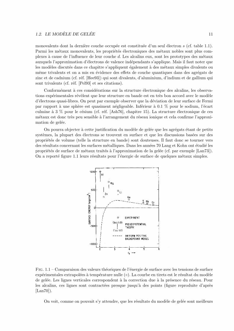
On pourra objecter a cette justification du modele de gelee que les agregats etant de petitssystemes, la plupart des electrons se trouvent en surface et que les discussions basees sur desproprietes de volume (telle la structure en bande) sont douteuses. Il faut donc se tourner versdes resultats concernant les surfaces metalliques. Dans les annees 70 Lang et Kohn ont etudie lesproprietes de surface de metaux traites a l’approximation de la gelee (cf. par exemple [Lan73]).On a reporte figure 1.1 leurs resultats pour l’energie de surface de quelques metaux simples.
Fig. 1.1 – Comparaison des valeurs theoriques de l’energie de surface avec les tensions de surfaceexperimentales extrapolees a temperature nulle (◦). La courbe en tirets est le resultat du modelede gelee. Les lignes verticales correspondent a la correction due a la presence du reseau. Pourles alcalins, ces lignes sont contractees presque jusqu’a des points (figure reproduite d’apres[Lan70]).
On voit, comme on pouvait s’y attendre, que les resultats du modele de gelee sont meilleurs

12 CHAPITRE 1. AGREGATS DE METAUX SIMPLES
pour les faibles densites, mais il y a un assez bon accord pour tous les alcalins (a l’exception dulithium). L’accord est ameliore par l’inclusion de pseudo-potentiels qui decrivent l’interactiondes electrons avec le substrat ionique : les ions sont alors situes sur les sites d’un reseau regulieroccupant un demi-espace (on sort donc de l’approximation de gelee) et interagissent avec leselectrons via un pseudo-potentiel et non via le potentiel coulombien nu. Cela est cense decrirede maniere effective l’influence des electrons de cœur et cela permet d’eviter la catastrophed’une energie de surface negative (cf. figure 1.1). Il est important de remarquer que les alcalinssont tres peu sensibles a l’arrangement du reseau ionique : pour eux, l’ecart entre les resultatsobtenus avec differents types de reseaux cristallins est presque nul.
En resume, les resultats de Lang et Kohn, tout en confirmant l’approximation de gelee,illustrent aussi les limitations du modele. Effectivement, malgre ses succes dans la descriptiondes effets de couche (cf. table 1.2 ci-apres), le modele de gelee n’est pas la panacee de la physiquedes agregats de metaux simples. Il trouve par exemple ses limites dans le traitement de la reponseoptique : l’emplacement precis de la resonance de plasmon, le profil de la section efficace et sadependance en temperature ne sont correctement decrits que par des modeles qui prennentexplicitement en compte la structure ionique de l’agregat.
1.3 Champ moyen – Effets de couche quantiques
Les effets de couche quantiques sont toujours associes a l’approche de champ moyen. Lescouches correspondent a des regroupements periodiques de niveaux dans le spectre des etatspropres du champ moyen.
Des effets de couche quantiques furent en premier lieu observes dans l’atome ou les electronsoccupent les couches successives dans le champ cree par le noyau (couches K, L, M , etc . . .).Les effets de couche en physique des agregats sont cependant plus proches de ceux observesen physique nucleaire, car le champ moyen electronique est principalement un champ auto-coherent, comme celui auquel sont soumis les nucleons du noyau. En effet, le champ exterieurcree par les ions est compense par le terme direct de l’interaction electronique et, dans uneapproche a la Hartree-Fock par exemple, c’est alors principalement le terme d’echange qui creele champ moyen.
La justification de l’approche de champ moyen dans les agregats repose sur le modele degelee. On peut, dans le cadre de ce modele, traiter les electrons de valence par exemple par lamethode de la fonctionnelle de la densite (c’est ce qu’a fait Ekardt dans son article de 1984 citeplus haut [Eka84]). Dans cette methode, l’energie du systeme d’electrons de valence est ecritecomme une fonctionnelle de la densite electronique n(x ) [Hoh64], typiquement de la forme :
E[n(x )] = T [n(x )] − e2∫
d3xd3x′n(x )nions(x
′)
|x − x ′| +e2
2
∫
d3xd3x′n(x )n(x ′)
|x − x ′| + EXC [n(x )] .
(1.1)
Dans (1.1) T [n(x )] est l’energie cinetique d’un systeme d’electrons sans interaction et dedensite n(x ) (une approche simple consiste a l’ecrire en utilisant l’approximation de Thomas-Fermi, mais on peut l’exprimer en terme des fonctions propres individuelles qui sont alors desparametres variationnels [Koh65]). Le deuxieme terme de (1.1) represente l’interaction avecles ions du substrat (dans le modele de gelee, la densite ionique nions(x ) est proportionnellea Θ(R − |x |), R etant le rayon de l’agregat) et le troisieme terme est la partie directe de

1.3. CHAMP MOYEN – EFFETS DE COUCHE QUANTIQUES 13
l’interaction electron/electron. Le dernier terme represente de maniere phenomenologique lacontribution des energies d’echange et de correlation.
La minimisation de l’energie du systeme conduit a une equation auto-coherente, soit pourn(x ) (si T [n] est decrite par l’approximation de Thomas-Fermi), soit pour les fonctions d’ondeindividuelles ϕi(x ) (dans le cas ou T [n] est exprimee en fonction des ϕi, [Koh65]) dans unchamp moyen de la forme :
V (x ) = e2∫
d3x′n(x ′) − nions(x
′)
|x − x ′| +δEXC
δn(x ). (1.2)
C’est la quantification des niveaux dans ce champ auto-coherent qui conduit a des effetsde couche. Bien-sur, si l’on a resolu le probleme a l’approximation Thomas-Fermi, l’energie dusysteme ne revelera pas d’effets de couche. Mais il faut noter qu’a partir du seul ingredientde la solution Thomas-Fermi (soit nTF (x )) on peut obtenir l’energie du systeme traite sanscette approximation avec une precision de l’ordre O(n − nTF )2 et ainsi retrouver les effets decouche (c’est un resultat de la methode des corrections de couche de Strutinsky, cf. par exemple[Bra72]).
D’ailleurs, dans l’esprit de la methode des corrections de couche, on peut aller plus loinque la formulation (1.1) dans la simplification du traitement du systeme des N electrons etrepresenter l’energie du systeme sous la forme :
E[n] = EGL[n] + Eshell[n] , (1.3)
ou EGL est une contribution de goutte liquide a l’energie du systeme (avec un terme de volume,de surface, etc . . .) qui utilise des parametres phenomenologiques (energie par particule dans lesysteme infini, tension de surface etc . . .). Eshell est une correction de couche a EGL. Elle peutetre obtenue comme la contribution oscillante a l’energie totale d’un systeme deN electrons dansun champ exterieur qui imite la forme de V (x )2. Ainsi, Nishioka et al. [Nis90] ont imite avec unpotentiel de Woods-Saxon le champ moyen auto-coherent obtenu par Ekardt dans [Eka84] ; plusrecemment, Yannouleas et Landman ont obtenu de bons accords quantitatifs avec l’experiencedans la region des petites tailles (N ≤ 50) en utilisant un simple potentiel harmonique anisotrope[Yan95].
Afin d’illustrer la qualite des resultats de l’approche de fonctionnelle de la densite (1.1) et dela methode de correction de couche (1.3), on a reproduit dans la table 1.2 la valeur des nombresmagiques obtenus pour des agregats alcalins de taille N ≤ 1500. Les trois premieres colonnesrepresentent les resultats des groupes experimentaux de Stuttgart [Mar90], Copenhague [Ped91]et Orsay [Bre93]. Dans les deux dernieres colonnes sont reportes les resultats d’un modele simplede cavite spherique (discute en detail au chapitre 2) puis d’un traitement theorique d’un modelede gelee spherique par la methode de fonctionnelle de la densite [Gen91].
On voit qu’il y a un bon accord sur toute la gamme de tailles entre l’experience et lesapproches theoriques. Il est etonnant de remarquer que le modele simple de la cavite spheriquereproduit les nombres magiques experimentaux aussi correctement que l’approche plus elaboreedu modele de gelee traite au moyen d’une fonctionnelle de la densite. Cela indique que le champmoyen obtenu par cette methode a beaucoup de similitudes avec un puits infini.
L’avantage d’une formulation de type (1.3) par rapport a une approche plus complexe estqu’elle permet de calculer les proprietes energetiques du systeme de N electrons en interaction a
2Voir l’allure typique de Eshell sur la figure 2.5 qui donne le resultat dans une cavite spherique.

14 CHAPITRE 1. AGREGATS DE METAUX SIMPLES
Na Stuttgart Na KBH Li Orsay Sphere FdD
2 2 2 28 8 8 820 20 20 2040 40 40 34 3458 58 58/70 58 5892 92 92 92 92138 138 138 138 138
198±5 198 198 186 186263±5 264 258 254 254341±5 344 336 338 338443±5 442 440 440 440557±5 554 546 542/556 542/556700±15 680 710 612/676 676840±15 800 750/820 748/832 758/832
970 910 912 9121040±20 1120 1065/1160 1074 1074/11001220±20 1310 1270/1370 1284 12841430±20 1500 1510 1502 1502
Tab. 1.2 – Nombres magiques dans les agregats alcalins. Les colonnes Na Stuttgart, Na KBH etLi Orsay referent repectivement aux resultats des refs. [Mar90], [Ped91] et [Bre93]. La quatriemecolonne repesente les nombres magiques dans un modele de cavite spherique et la colone FdD,les resultats de fonctionelle de la densite de Genzken et Brack [Gen91].
l’approximation des particules independantes. Les succes qualitatifs (cf. table 1.2) et quantitatifs(cf. ref. [Yan95]) de cette approche justifient a posteriori le modele de champ moyen (et au dela,le modele de gelee) utilise pour la description de la structure electronique des agregats de metauxsimples.
Bien sur, les memes reserves que l’on avait faites a la fin de la section precedente pourle modele de gelee s’appliquent ici aux modeles du type (1.3) : l’approche du champ moyenexterieur n’est pas adaptee a l’etude de toutes les proprietes des agregats metalliques. Elleserait par exemple incapable de decrire des phenomenes collectifs.
Notons enfin que les modeles que nous venons de presenter dans cette section semblent auxantipodes des conceptions a la Kubo qui mettent en avant l’effet du desordre (cf. section 1.1).Une possible conciliation des deux approches sera presentee au chapitre 4 (et ref. [Pav98]).

Chapitre 2
Formule des traces
Dans ce chapitre, nous allons presenter la formule des traces qui est un outil permettantd’exprimer – dans la limite semiclassique – la densite de niveaux d’un systeme quantique unique-ment a partir d’informations contenues dans la dynamique classique du syteme. Cette formuleconcerne les systemes hamiltoniens (auquels nous nous restreindrons dans tout ce memoire) eta ete obtenue pour la premiere fois en 1971 par Gutzwiller pour un systeme chaotique generique[Gut71] et dans le cas d’une particule dans un billard par Balian et Bloch [Bal72]. Le cas d’unsysteme integrable generique a ete ensuite traite par Berry et Tabor [Ber76]. Notons egalementqu’en 1974, Balian et Bloch ont obtenu, pour des potentiels analytiques, une formule des tracesformellement exacte [Bal74].
Cette approche repose sur la connaissance des orbites periodiques (OPs) classiques dusysteme et est parfois appelee “developpement en orbites periodiques”. Il est a noter que l’onpeut trouver dans la litterature de notables precurseurs. On peut considerer que la plus ancienneversion est la formule sommatoire de Poisson, qui s’interprete comme une formule des traces pourle laplacien sur un tore. Dans la galerie des ancetres il y a egalement la formule que l’on obtientpour la densite de zeros non triviaux de la fonction ζ de Riemann a partir du produit d’Eulerde cette fonction (cf. [Gut90], section 17.9). Le traitement par Landau en 1939 de la reponsemagnetique d’un gaz d’electrons ([Lan84], section 60) repose lui aussi sur un developpementen OPs qui se generalise aisement au traitement plus realiste des oscillations de de Haas–vanAlphen ([Lif86], section 63). Dingle a egalement derive en 1951 une formule des traces decrivantle mouvement d’un electron a l’interieur d’un cylindre et d’une sphere en presence d’un champmagnetique uniforme [Din52]. Enfin, Selberg en 1956 a obtenu une formule des traces exactepour le mouvement d’une particule sur la surface de Poincare (cf. par exemple [Bal86]).
Des les annees 70, les travaux de Gutzwiller et de Balian et Bloch ont recu l’attentiondes mathematiciens. Colin de Verdiere [Col73] a donne une formule synoptique exprimant uneversion regularisee de la densite de niveaux du laplacien sur une variete riemanienne en fonctiondes longueurs des geodesiques periodiques. Dans la meme veine, Chazarain [Cha74] a montreque les singularites de certaines fonctions de traces sur des varietes riemaniennes etaient situeessur les longueurs des geodesiques periodiques. Ensuite Duistermaat et Guillemin [Duis75] ontdonne la forme explicite du prefacteur associe a ces singularites, en accord avec le resultat deGutzwiller [Gut71] (on peut trouver dans la ref. [Gut97] un compte rendu par Gutzwiller del’historique de la formule des traces, et dans [Col94] des references plus recentes sur les travauxde la communaute mathematique).
15

16 CHAPITRE 2. FORMULE DES TRACES
2.1 Un cas unidimensionnel simple
On peut donner une illustration simple d’un developpement en orbites periodiques grace al’exemple du puits carre unidimensionnel. On considere le mouvement d’une particule astreintea se deplacer sur l’axe Ox, soumise a l’action d’un potentiel exterieur V (x) nul pour x ∈]0, a[et infini partout ailleurs. Le hamiltonien du systeme est H = p2/(2m) + V (x) et l’equation deSchrodinger pour cette particule s’ecrit (hk =
√2mE) : ψ′′(x)+k2 ψ(x) = 0, avec les conditions
aux limites ψ(0) = ψ(a) = 0.
Les niveaux peuvent etre determines semi-classiquement grace a la quantification de Bohr-Sommerfeld en imposant sur une periode du mouvement classique
1
2π
∮
p dx = nh ou n = 1, 2, . . . (2.1)
On obtient alors les niveaux propres du systeme kn = nπ/a (il est a noter qu’ici l’approxi-mation semiclassique est exacte).
Une autre methode consiste a utiliser la formule sommatoire de Poisson. Cette formulepermet d’exprimer la densite de niveaux ρ(k) (ρ(k)
def=
∑+∞ν=1 δ(k−kν)) sous la forme d’un terme
moyen auquel s’ajoute une somme de termes oscillants :
ρ(k) =+∞∑
ν=1
δ(k − νπ
a) =
a
π+
2 a
π
+∞∑
n=1
cos(2na k) (2.2)
Dans la formule (2.2) on n’associe pas a chaque niveau une orbite fermee que l’on quantifiecomme dans la formule de Bohr-Sommerfeld, mais a la densite de niveaux totale correspondune somme sur les orbites periodiques du systeme (leur longueur etant de la forme 2na avecn = 1, 2, . . .). Lorsque les contributions du terme de droite de (2.2) interferent constructivement,on obtient un pic delta et k est une valeur propre.
Pour des systemes a un degre de liberte, on peut toujours obtenir une formule similaire al’equation (2.2), mais dans quelques cas seulement (tel celui que nous venons de traiter), cetteformule est exacte.
2.2 Systeme a D degres de liberte (D ≥ 2)
Dans le cas unidimensionnel precedent, la quantification semiclassique pouvait etre obtenueindifferemment par la methode de Bohr-Sommerfeld ou par un developpement en OPs. Endimension D ≥ 2 la methode de Bohr-Sommerfeld est appelee methode EBK (d’apres Einstein,Brillouin et Keller) ou quantification par les tores. Elle n’est utilisable que pour des systemesintegrables, cela se comprend grace a l’ebauche de demonstration suivante.
2.2.1 Methode EBK
Un systeme integrable a D degres de liberte est caracterise par l’existence de D constantesdu mouvement independantes qui “commutent” entre elles (c.a.d. que leur crochet de Poissonest nul). L’une de ces constantes du mouvement est bien sur l’energie, les D − 1 autres com-mutant avec H, ce sont des quantites conservees au cours du mouvement. Donc la dynamique
2.2. SYSTEME A D DEGRES DE LIBERTE (D ≥ 2) 17
dans l’espace des phases (qui est de dimension 2D) n’explore pas toute la surface d’energie(caracterisee par l’equation H( p , q ) = Cste, celle-ci est de dimension 2D − 1), mais seulementun sous-domaine de dimension D dont on peut montrer qu’il a la topologie d’un tore (cf. e.g.
l’expose [Ber78] ou le traite [Arn97]).
Si, pour un jeu donne desD constantes du mouvement, on essaie de definir – dans le cadre del’approximation semiclassique – une fonction d’onde stationnaire associee au tore correspondantde l’espace des phases, on ecrira [Kel58, Per77, Bra97]
Ψsc( q ) =R
∑
r=1
Ar( q ) eiSr( q )/h . (2.3)
La sommation sur r correspond a la topologie du tore. En effet, un ansatz du type (2.3) –sans la somme sur r – reporte dans l’equation de Schrodinger, donne a l’ordre dominant en h unefonction S( q ) qui est solution de l’equation de Hamilton-Jacobi stationnaire H(∂S/∂ q , q ) = E
et on obtient S( q ) =∫ q
q 0 p ( q ′).d q ′ (ou l’integrale est effectuee sur le tore de l’espace des phasesconsidere et q 0 est un point de reference arbitraire sur ce tore). Or, a cause de la topologie dutore, cette fonction est multivaluee – d’ou l’ansatz (2.3) – et on obtient pour la branche r deS : Sr( q ) =
∫ qq 0 p r( q
′).d q ′, ou p r( q ) est determine par l’une des R intersections du tore avec
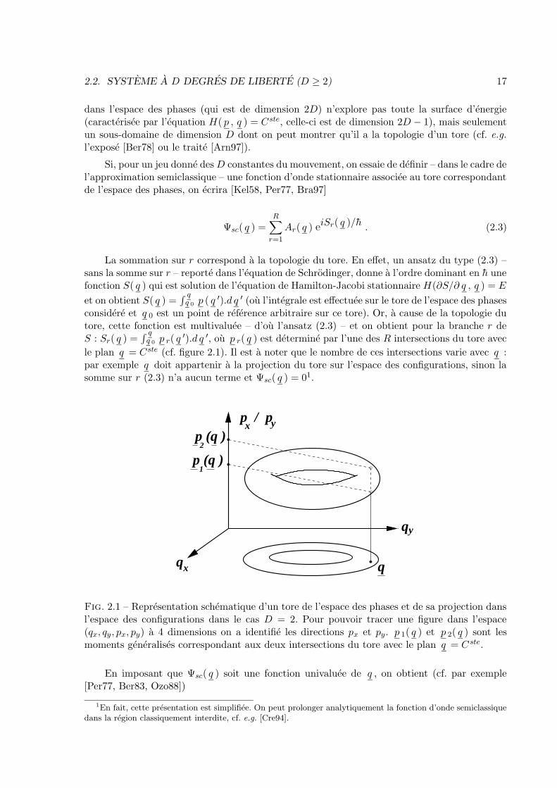
le plan q = Cste (cf. figure 2.1). Il est a noter que le nombre de ces intersections varie avec q :par exemple q doit appartenir a la projection du tore sur l’espace des configurations, sinon lasomme sur r (2.3) n’a aucun terme et Ψsc( q ) = 01.
q
q
x
y
p (q )
p (q )2
q
p / px y
1
Fig. 2.1 – Representation schematique d’un tore de l’espace des phases et de sa projection dansl’espace des configurations dans le cas D = 2. Pour pouvoir tracer une figure dans l’espace(qx, qy, px, py) a 4 dimensions on a identifie les directions px et py. p 1( q ) et p 2( q ) sont lesmoments generalises correspondant aux deux intersections du tore avec le plan q = C ste.
En imposant que Ψsc( q ) soit une fonction univaluee de q , on obtient (cf. par exemple[Per77, Ber83, Ozo88])
1En fait, cette presentation est simplifiee. On peut prolonger analytiquement la fonction d’onde semiclassiquedans la region classiquement interdite, cf. e.g. [Cre94].
18 CHAPITRE 2. FORMULE DES TRACES
∮
γj
p ( q ).d q = 2π nj h (j = 1 . . .D) , (2.4)
ou nj est un entier et γj est un des D chemins fermes irreductibles du tore (dans (2.4) le momentp ( q ) est choisi par continuite le long de γi dans un des R feuillets). Cette condition a ete obtenuesous cette forme pour la premiere fois par Einstein en 1917. La formule (2.4) suffit pour notrediscussion, mais il faut noter qu’elle n’est pas tout a fait exacte : elle doit etre affinee pour tenircompte d’eventuelles singularites de l’amplitude A( q )2 et cela correspond a introduire dans lesconditions de quantification (2.4) un indice supplementaire, l’indice de Maslov.
Ce qui est important pour la presente discussion c’est la structure tres particuliere de ladynamique d’un systeme integrable dans l’espace des phases : les mouvements s’effectuent surdes tores. Si l’on ajoute au hamiltonien une perturbation qui en brise l’integrabilite, les toresdisparaissent. La maniere tres complexe dont ils sont brises est decrite par le theoreme KAM,mais il est clair par exemple, comme l’avait deja remarque Einstein en 1917 (cite dans [Per77]),que la quantification de Bohr-Sommerfeld ne se generalise pas au cas extreme des systemesergodiques qui explorent toute la surface d’energie : dans ce cas on n’a pas un nombre fini defonctions p r( q ). On doit donc avoir un systeme integrable pour utiliser la quantification EBK.
2.2.2 Formule des traces
Contrairement a ce qui se passe pour la quantification par les tores, on peut, meme pour dessystemes tres chaotiques, ecrire la densite de niveaux semiclassique sous une forme qui rappelle(2.2) :
ρ(E)def=
+∞∑
ν=1
δ(E − Eν) = ρTF (E) + ρosc(E) , (2.5)
ou ρTF (E) est une fonction reguliere “sans accident” de l’energie que l’on appelle terme deThomas-Fermi (ou developpement de Weyl dans le cas d’un billard). A l’ordre dominant, ρTF (E)correspond simplement au comptage d’etats sur la surface d’energie et s’ecrit :
ρTF (E) =
∫
dDp dDq
(2πh)Dδ(E −H( p , q )) + . . . (2.6)
Les termes suivants dans l’expression de ρTF correspondent a des corrections de bord dansle potentiel et sont sous-dominants en h. Le terme a/π dans le membre de droite de (2.2) estl’analogue de (2.6) dans le cas simplifie du puits carre (dans ce cas il faut noter que ρ(E) =mρ(k)/(h2k)).
Le terme oscillant de la formule (2.5) s’ecrit lui dans le cas general :
ρosc(E) = Re∑
n=OP
Cn(E) eiSn(E)/h + . . . (2.7)
ou la somme est effectuee sur toutes les OPs du systeme (reperees par l’indice n). La formule (2.7)est une somme de termes qui oscillent rapidement (h est “petit”) multiplies par des amplitudes (a
2Comme S( q ), cette amplitude est multivaluee ; elle a la meme structure en feuillets que S, en outre ellediverge sur les points de branchement.
2.2. SYSTEME A D DEGRES DE LIBERTE (D ≥ 2) 19
priori complexes) Cn(E) qui dependent peu de l’energie. Sn(E) =∮
n p .d q est l’action le long del’OP consideree. C’est cette formule qui est appelee formule des traces. Une version tres simplifieede (2.7) est donnee par la formule (2.2) : dans ce cas Cn(E) = 2ma/(πh2k) = a/(πh)
√
2m/Eet Sn(E) = hkLn ou Ln = 2na est la longueur de l’OP n.
2.2.3 Synopsis de la demonstration de la formule des traces
Sans etablir rigoureusement la formule (2.7) (la derivation est donnee dans [Gut89] et, d’unpoint de vue plus mathematique, dans [Col94]) on peut expliquer par des arguments simplesl’apparition des OPs du systeme classique dans l’expression semiclassique de la densite d’etat.
L’ingredient de base est la fonction de Green du systeme, solution de
{
E −H(−ih∇ q , q )}
G( q , q ′, E) = δ( q − q ′) . (2.8)
G( q , q ′, E) s’exprime en terme des fonctions propres du systeme :
G( q , q ′, E) =+∞∑
ν=1
ψν( q )ψ∗ν( q
′)
E − Eν, (2.9)
et sur la base de la formule (2.9), on ecrit la densite de niveaux sous la forme :
ρ(E) =+∞∑
ν=1
δ(E − Eν) = − 1
πIm
∫
dDq limε→0+
G( q , q , E + iε) . (2.10)
Donc, si l’on arrive a obtenir une formule semiclassique pour G en terme d’une sommesur des trajectoires classiques, on peut esperer aboutir a une expression de type (2.7) : en effetG( q , q , E) est le propagateur pour des trajectoires d’energie E partant de q et aboutissant aq : donc, toutes les orbites fermees contribuent a (2.10). On va plus loin justifier que, parmi cesorbites, les orbites periodiques jouent un role preponderant.
L’expression semiclassique de G est obtenue a partir du propagateur K( q , q ′, t) qui estdefini pour t > 0 comme la solution de l’equation de Schrodinger dependante du temps avec lacondition initiale limt→0K( q , q ′, t) = δ( q − q ′). L’approximation semiclassique de K s’ecrit :
Ksc( q , q′, t) =
∑
q ′→ q
An( q , q ′, t) eiRn( q , q ′, t)/h , (2.11)
ou Rn( q , q ′, t) =∫ t0 L(x , x , τ)dτ est l’integrale du lagrangien le long de l’orbite classique
(reperee par n dans (2.11)) allant de q ′ a q en un temps t. La sommation etant effectueesur toutes les orbites classiques n. An( q , q ′, t) est proportionnel a la densite de probabilite detrouver le systeme au temps t dans l’element de volume dDq sachant qu’il etait en dDq′ a t = 0.Cette formule a ete obtenue pour la premiere fois par Van Vleck en 1928 et generalisee parGutzwiller en 1967 dans [Gut67]. Elle est tres naturelle si l’on exprime K grace au formalismede l’integrale de chemin :
K( q , q ′, t) =
∫
[D x (τ)] exp
{
i
h
∫ t
0L(x , x , τ)dτ
}
. (2.12)

20 CHAPITRE 2. FORMULE DES TRACES
La phase de l’integrale (2.12) est stationnaire pour les trajectoires classiques et vautRn( q , q ′, t). Donc la formule de Van Vleck (2.11) correspond juste a une approximation dela phase stationnaire pour (2.12).
L’etape suivante consiste a ecrire G comme la transformee de Laplace du propagateur :
G( q , q ′, E) =1
ih
∫ +∞
0eiEt/h K( q , q ′, t)dt . (2.13)
Et a nouveau, une analyse en phase stationnaire permet d’obtenir une formule semiclassiquedu type :
Gsc( q , q′, E) =
∑
q ′→ q
Bn( q , q ′, E) eiSn( q , q ′, E)/h , (2.14)
ou Sn = Rn + Et =∫ q
q ′ p .d x est l’action le long de la trajectoire n, d’energie E, allant de q ′
a q .
A ce stade nous avons, comme promis, exprime la fonction de Green comme une somme surdes trajectoires classiques. Enfin, au moment de prendre la trace sous la forme d’une integrale∫
dDq dans la formule (2.10), une nouvelle condition de phase stationnaire impose (d’apresl’expression semiclassique (2.14) de la fonction de Green) :
∂S
∂ q− ∂S
∂ q ′
∣
∣
∣
∣
∣
q = q ′
= 0 soit p ′ = p en q ′ = q . (2.15)
Cette derniere equation correspond a une orbite periodique. Une analyse delicate du com-portement des integrales permet d’obtenir le prefacteur correspondant a cette derniere approxi-mation de phase stationnaire et d’ecrire ainsi la densite de niveaux sous la forme (2.7).
2.3 Interet pratique de la formule des traces
On ne peut obtenir de developpement en OPs coherent que dans le cas d’un systemeintegrable [Ber76] ou d’un systeme fortement chaotique ou toutes les OPs sont isolees et oul’analyse en phase stationnaire de l’integrale (2.10) est justifiee. Pour les systemes mixtes dontl’espace des phases comprend des regions chaotiques et des ılots integrables, on doit utiliser desapproximations uniformes et il faut alors traiter les orbites presque au cas par cas.
Lorsque l’on veut, a partir de la formule des traces, determiner des niveaux individuels, sil’on ecarte le cas d’un systeme integrable, il n’est possible de determiner le grand nombre d’OPsrequis pour l’implementation de la formule que dans le cas d’un systeme fortement chaotique,lorsque l’on peut etablir une dynamique symbolique finie (i.e. pour certains systemes K). Cetype de recherche a ete poursuivi par Gutzwiller [Gut80], Cvitanovic [Cvi89], Steiner [Sie91b],Bogomolny [Bog93] et leurs collaborateurs, mais en pratique il n’est possible de determiner decette maniere que quelques dizaines de niveaux propres. La resolution numerique de l’equation deSchrodinger est alors beaucoup plus efficace. Ainsi, dans la ref. [Sie91a], Sieber ayant determineles 500 000 premieres OPs d’un billard en forme d’hyperbole, a pu calculer environ 50 niveauxpropres a partir de la formule des traces (a comparer aux 600 niveaux qu’il avait calcules
2.3. INTERET PRATIQUE DE LA FORMULE DES TRACES 21
numeriquement). Ce type d’etude a plutot un interet theorique se rapportant aux delicatesproprietes de convergence de la formule des traces.
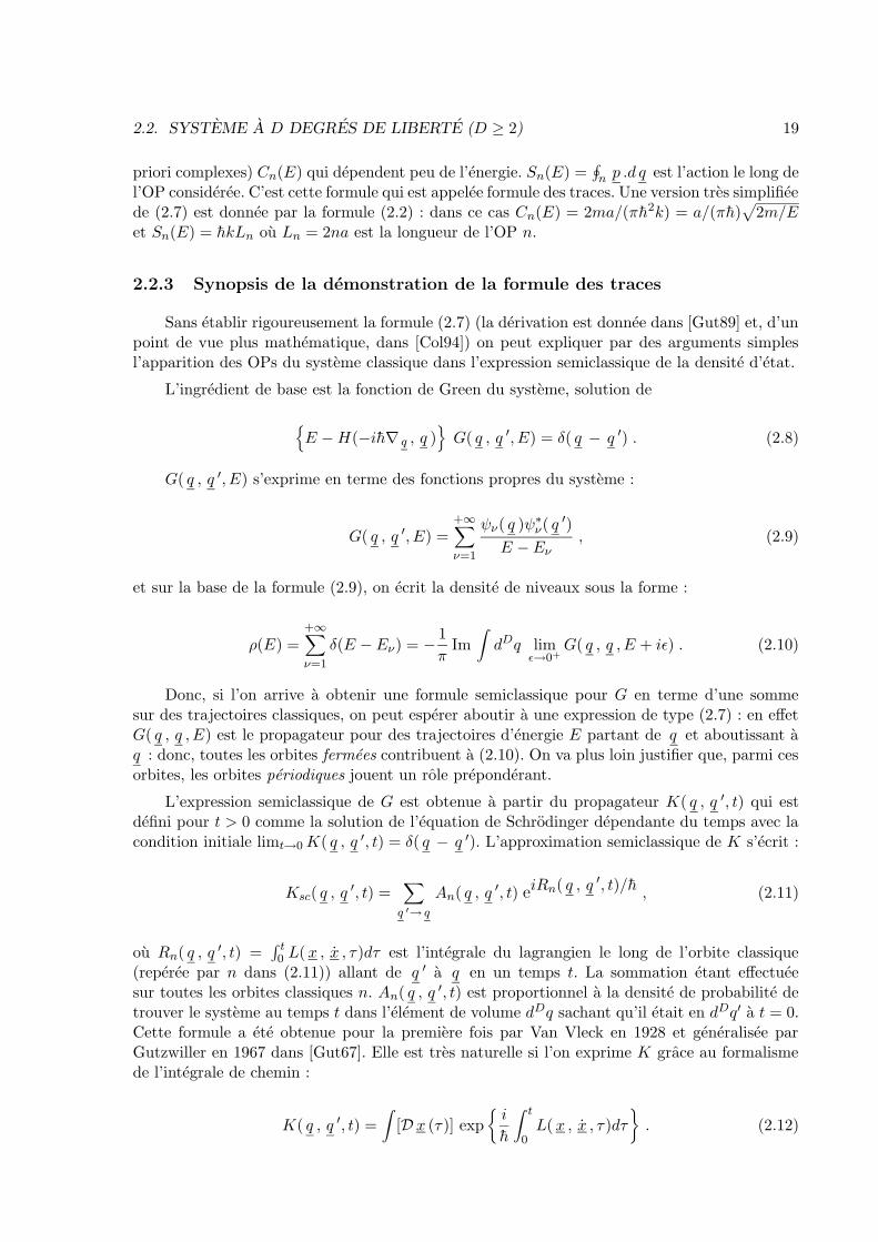
Par contre, si l’on ne s’interesse pas aux niveaux individuels, les quelques orbites les pluscourtes suffisent a interpreter l’allure generale de la densite de niveaux. Ainsi, si l’on ignore lesdetails du spectre inferieurs a une echelle ∆E, seules les orbites ayant une periode inferieure ah/∆E sont utiles3. C’est illustre sur la figure 2.2.
�
- ∆E
Periode
regime“ultra-quantique”
u
u
regime de la formuledes traces
regime Thomas-Fermi
u
u
Ec = h/tdenergie de Thouless
td : periode de l’OPla plus courte
δ : espacementmoyen
th = h/δtemps de Heisenberg
Fig. 2.2 – Representation schematique du domaine d’“utilisabilite” de la formule des traces.
Si l’on s’interesse aux proprietes “a un corps” de la densite de niveaux (et non pas auxcorrelations spectrales), la formule des traces usuelle n’est pas necessaire si ∆E est trop grand :dans ce cas, la simple donnee de ρTF (E) suffit pour le niveau de precision requis. Cette valeurlimite superieure de ∆E correspond a l’energie de Thouless du systeme qui vaut h/td, td etantle temps typique de traversee du systeme (c’est par exemple la periode de l’OP la plus courte).Pour un agregat modelise par un billard tridimensionnel, td est de l’ordre de L/vF = mL/(hkF )ou L est la taille typique du billard et vF la vitesse de Fermi des electrons.
La valeur inferieure de ∆E en dessous de laquelle la formule des traces n’apporte plus d’in-formation pertinente est l’espacement entre niveaux δ. Cela correspond a des orbites de periodeth = h/δ, le temps de Heisenberg. Pour un billard tridimensionnel modelisant un agregat, ona, au niveau de Fermi, δ ∼ (L
√m/h)3
√EF et on obtient th ∼ L3kF/h ∼ td(LkF )2. La taille
L de l’agregat croıt comme rSN1/3 ∼ N1/3/kF (rS est le rayon de Wigner-Seitz, pour un gaz
d’electrons rS = k−1F (9π/4)1/3) donc pour un billard contenant 1000 atomes, LkF ∼ N1/3 = 10
et th ∼ 100 td. Pour determiner les niveaux individuels et donc etudier le spectre jusqu’a desdetails de l’ordre de ∆E = δ il faut alors utiliser toutes les OPs jusqu’a une longueur de l’ordrede 100 fois l’OP la plus courte. Si cette limite est eventuellement atteignable pour un billardintegrable, elle est hors de portee pour des systemes chaotiques ou le nombre d’orbites croıtexponentiellement avec leur taille.
Dans les travaux presentes ci-apres la formule des traces sera utilisee pour discuter l’al-lure du spectre a une particule sur des echelles ∆E assez grandes : l’effet de couche dans lesagregats correspond a une precision de l’ordre de Ec ou Ec/2 et quelques orbites seulement suf-fisent a determiner l’allure du spectre a cette echelle. En outre, lors de la comparaison avec lesexperiences, les details du spectre peuvent etre effaces par des effets de temperature, de moyen-nage sur des configurations desordonnees etc, . . .Ces effets seront discutes dans le chapitre 4.
3Cela se voit par exemple en convoluant la formule (2.7) avec une gaussienne de largeur ∆E.

22 CHAPITRE 2. FORMULE DES TRACES
2.4 La formule des traces dans la sphere – Supercouches
Dans cette section nous allons illustrer l’utilisation de la formule des traces en l’appliquant al’etude du spectre dans un billard tridimensionnel spherique. On discutera egalement l’occurencedu phenomene de supercouche qui a ete predit par Balian et Bloch en 1972 [Bal72] et misen evidence pour la premiere fois dans les agregats de sodium par l’equipe de Bjørnholm aCopenhague en 1991 [Ped91].
Selon la formule (2.5) on ecrit la densite de niveaux dans la sphere comme la somme d’unterme de Thomas-Fermi et d’un terme oscillant. Le terme de Thomas-Fermi dans la sphere estconnu depuis longtemps (cf. e.g. [Bal76]) et a la forme :
ρTF (k) =2
3πR3k2 − 1
2R2k +
2
3πR+ . . . . (2.16)
Le terme oscillant a ete determine pour la premiere fois par Balian et Bloch [Bal72]. Lesorbites periodiques de la sphere sont des polygones plans caracterises par 2 indices n et t : nest le nombre de rebonds de l’OP sur la frontiere et t le nombre de tours que l’OP effectueautour de l’origine (n ≥ 2 t). Les orbites periodiques les plus courtes sont representees sur lafigure 2.3. Une orbite caracterisee par les indices (n, t) a une longueur Ln,t = 2nR sin(πt/n).Ainsi le triangle et le carre ont des longueurs L3,1 = 3
√3R ' 5.20R et L4,1 = 4
√2R ' 5.66R.
L’expression detaillee de ρosc(k) est rappelee dans la reference [Pav98] reproduite au chapitre 4.
Fig. 2.3 – Quelques unes des OPs les plus courtes dans la sphere (d’apres la ref. [Bal72]). Endessous de chaque OP sont reproduits ses indices (n, t) (cf. texte).
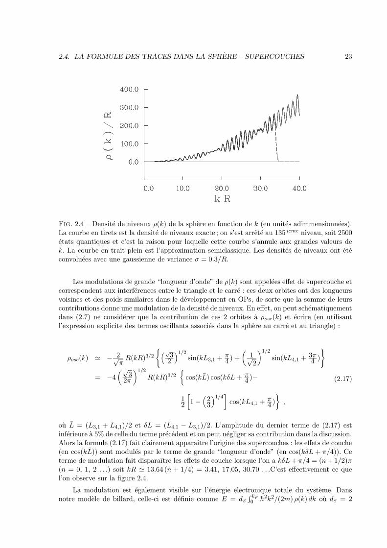
On peut, pour la sphere, tester la precision de la formule semiclassique (2.7) en la comparantavec la densite de niveaux exacte qui est constituee d’une suite de pics de Dirac. Afin de nepas avoir a inclure trop d’orbites (cf. la discussion de la section precedente) on a compare surla figure 2.4 les densites de niveaux exacte et semiclassique convoluees avec une gaussienne devariance σ = 0.3/R. Les deux courbes se recouvrent presque exactement. Les oscillations de ρ(k)correspondent a des regroupements quasi-periodiques de niveaux, ce sont les effets de couche.Ils sont dus aux oscillations causees par l’orbite la plus courte : l’orbite triangulaire (l’orbitediametrale L2,1 a une contribution sous-dominante, cf. la discussion de l’appendice A de la ref.[Pav98]). Ainsi, une accumulation de niveaux autour d’un vecteur d’onde k comprend environπρTF (k)/L3,1 ' 2(Rk)2/(9
√3) niveaux.
2.4. LA FORMULE DES TRACES DANS LA SPHERE – SUPERCOUCHES 23
Fig. 2.4 – Densite de niveaux ρ(k) de la sphere en fonction de k (en unites adimmensionnees).La courbe en tirets est la densite de niveaux exacte ; on s’est arrete au 135 ieme niveau, soit 2500etats quantiques et c’est la raison pour laquelle cette courbe s’annule aux grandes valeurs dek. La courbe en trait plein est l’approximation semiclassique. Les densites de niveaux ont eteconvoluees avec une gaussienne de variance σ = 0.3/R.
Les modulations de grande “longueur d’onde” de ρ(k) sont appelees effet de supercouche etcorrespondent aux interferences entre le triangle et le carre : ces deux orbites ont des longueursvoisines et des poids similaires dans le developpement en OPs, de sorte que la somme de leurscontributions donne une modulation de la densite de niveaux. En effet, on peut schematiquementdans (2.7) ne considerer que la contribution de ces 2 orbites a ρosc(k) et ecrire (en utilisantl’expression explicite des termes oscillants associes dans la sphere au carre et au triangle) :
ρosc(k) ' − 2√πR(kR)3/2
{
(√32
)1/2sin(kL3,1 + π
4 ) +
(
1√2
)1/2
sin(kL4,1 + 3π4 )
}
= −4
(√3
2π
)1/2
R(kR)3/2
{
cos(kL) cos(kδL+ π4 )−
12
[
1 −(
23
)1/4]
cos(kL4,1 + π4 )
}
,
(2.17)
ou L = (L3,1 + L4,1)/2 et δL = (L4,1 − L3,1)/2. L’amplitude du dernier terme de (2.17) estinferieure a 5% de celle du terme precedent et on peut negliger sa contribution dans la discussion.Alors la formule (2.17) fait clairement apparaıtre l’origine des supercouches : les effets de couche(en cos(kL)) sont modules par le terme de grande “longueur d’onde” (en cos(kδL + π/4)). Ceterme de modulation fait disparaıtre les effets de couche lorsque l’on a kδL+ π/4 = (n+ 1/2)π(n = 0, 1, 2 . . .) soit kR ' 13.64 (n + 1/4) = 3.41, 17.05, 30.70 . . .C’est effectivement ce quel’on observe sur la figure 2.4.
La modulation est egalement visible sur l’energie electronique totale du systeme. Dansnotre modele de billard, celle-ci est definie comme E = dS
∫ kF0 h2k2/(2m) ρ(k) dk ou dS = 2

24 CHAPITRE 2. FORMULE DES TRACES
est la degenerescence de spin et kF le niveau de Fermi. Ce dernier est determine en fonctiondu nombre N d’electrons par N = dS
∫ kF0 ρ(k) dk. Le rayon de la sphere modelisant l’agregat
et toutes les longueurs du systeme varient comme N 1/3 et il est usuel de representer la partieoscillante de l’energie totale4 en fonction de N1/3 : c’est ce qui a ete fait figure (2.5). On voitclairement sur cette figure l’effet de couche et de supercouche. La fin de la premiere supercoucheapparaıt a N 1/3 ' 8 ou 9 soit N ' 7005. C’est cette modulation qui a ete mise en evidenceexperimentalement pour la premiere fois dans des agregats de sodium par l’equipe de Bjørnholma Copenhague [Ped91]. Les supercouches ont egalement ete observees dans des agregats delithium par l’equipe de Brechignac a Orsay [Bre93] et dans le gallium par Pellarin et al. a Lyon[Pel93]. La fin de la deuxieme supercouche a egalement ete observee par cette derniere equipe[Pel95].
Fig. 2.5 – Partie oscillante Eshell de l’energie electronique totale en fonction de la taille N del’agregat. Eshell est exprimee en unites de l’energie de Fermi εF du systeme infini. Les valeursde N correspondant aux minima de Eshell sont les nombres magiques de la sphere.
On peut noter ici, qu’apres les travaux de Balian et Bloch, l’interet physique du phenomenede supercouche a ete egalement remarque par Strutinsky et Magner [Str75, Str76] qui le dis-cutent precisement dans les termes de l’equation (2.17). Ces auteurs partent de l’expression dupropagateur (2.11) et en suivant un schema tres similaire a celui de la section 2.2.3 discutentles effets de couche dans differents types de potentiels nucleaires. Notons, egalement dans lecontexte de la physique nucleaire, que Bohr et Mottelson [Boh75] ont eux aussi developpe uneinterpretation de l’effet de couche basee sur l’etude des orbites periodiques. Pour en finir avecles remarques historiques, il faut rappeler que l’analyse d’un spectre quantique en terme d’unesomme sur les OPs classiques a ete faite pour la premiere fois par Gutzwiller en 1971 [Gut71].
L’observation de supercouches donne des informations sur le champ moyen dans lequel sedeplacent les electrons : comme exemple extreme on peut verifier que la structure en supercouchen’existe pas dans un oscillateur harmonique ; on peut donc en conclure que dans un agregatmetallique, le champ moyen electronique est plus proche du puits spherique que de l’oscillateurharmonique. Nishioka, Hansen et Mottelson [Nis90] ont verifie que l’effet de supercouche subsistedans des champs moyens plus realistes que le puits spherique, puis Genzken et Brack [Gen91]ont egalement decrit le phenomene et sa dependance en temperature dans un traitement auto-coherent de la structure electronique. L’emplacement et la structure detaillee des supercouchesdependent de maniere cruciale des longueurs et des phases des orbites les plus courtes. C’est ce
4En accord avec les conventions habituelles dans le domaine des agregats, la partie oscillante de l’energieelectronique est notee Eshell (cf. chapitre 1).
5A l’ordre dominant on obtient la formule simple pour la valeur de N en fin de supercouche : N 1/3'
7.1 (n + 1/4) n = 0, 1, . . .
2.4. LA FORMULE DES TRACES DANS LA SPHERE – SUPERCOUCHES 25
qui a ete observe dans [Nis90] et qui est dramatiquement illustre dans le gallium, ou l’epaisseurde surface du potentiel provoque des changements de longueur de l’orbite triangulaire et ducarre qui resultent en un deplacement de la fin de la premiere supercouche qui est observeevers N ' 2500 electrons [Pel95]. Il est donc remarquable de noter que, malgre sa simplicite, lemodele du billard spherique predit avec precision la structure en couches et supercouches desagregats de sodium (cf. la table 1.2).
En conclusion de ce chapitre, il est interessant de mettre l’accent sur l’apport de l’eclairagesemiclassique a la thematique que nous venons d’exposer. La cavite spherique est un systemeintegrable bien connu et utilise comme cas modele depuis des decennies. L’etude semiclassique deson spectre a non seulement permis une interpretation geometrique simple de l’effet de couche,mais a aussi abouti a la decouverte du phenomene de supercouches et a son explication en termed’orbites periodiques. Ces resultats sont dus a Balian et Bloch et datent de 1972 [Bal72] alorsque les premieres etudes du spectre du laplacien dans la sphere semblent remonter a Poisson en1823 pour les fonctions propres (cite dans [Wat52], chapitre 1) et a Rayleigh en 1873 pour lespremiers niveaux propres6 [Str73].
6Watson ([Wat52], chapitre 15) cite egalement a ce sujet un traite de Schwerd publie en 1835.

26 CHAPITRE 2. FORMULE DES TRACES

Chapitre 3
Facettes et diffraction
3.1 Agregats metalliques facettes
3.1.1 Presentation des resultats experimentaux
Suivant l’experience fondatrice du groupe de Knight a Berkeley qui revela l’existence d’effetsde couche dans les agregats metalliques [Kni84], de nombreux groupes se sont attaches a etudierla structure electronique de ces agregats (cf. les references dans [Hee93]). On a ainsi mis trestot en evidence des effets de deformation sur les nombres magiques [Cle85] : la brisure de lasymetrie spherique des agregats entre deux fermetures de couche permet au systeme de diminuerson energie (en diminuant l’energie cinetique quantique des electrons). Ce point sera discute plusavant dans le chapitre suivant.
En 90 l’equipe de T. P. Martin a Stuttgart [Mar90] a obtenu des resultats sur les deforma-tions qui sont apparus comme une surprise dans la communaute des agregats metalliques. Cegroupe, disposant d’un spectrometre a temps de vol tres performant, a etudie les nombres ma-giques pour des agregats de sodium comprenant jusqu’a 22 000 atomes. Les premiers nombresmagiques, jusqu’a une taille N ∼ 1500, correspondent en gros aux nombres magiques de lasphere : ils croissent comme N 1/3 avec un espacement entre couches comparable a celui de lasphere (cf. la figure 2.5), bien que l’effet de supercouche soit absent1. Ensuite, pour N ≥ 1500,les nombres magiques croissent toujours comme N 1/3 mais avec un espacement entre couchesmultiplie par un facteur 2 environ. T. P. Martin et ses collaborateurs ont interprete ce chan-gement de pente en fonction de N 1/3 comme un changement de regime : les grands nombresmagiques correspondent, non pas a des fermetures de couches quantiques, mais a des empile-ments geometriques compacts de couches d’atomes. On a donc dans ce cas des deformationsd’origine non pas quantique mais geometrique. De tels empilements correspondent (dans le casd’une structure icosaedrique) a des nombres magiques de la forme :
Nn =1
3
(
10n3 − 15n2 + 11n− 3)
avec n = 1, 2, . . . (3.1)
On obtient alors une succession de nombres magiques d’origine geometrique en bon ac-cord avec les observations experimentales. Apres cette experience, des couches geometriquesont egalement ete observees dans des faisceaux d’agregats de metaux simples plus complexes
1Ceci a ete interprete par Clemenger comme un effet de deformation de multipolarite ` = 4 [Cle91], mais c’estegalement compatible avec une deformation icosaedrique, cf. ref. [Pav93].
27
28 CHAPITRE 3. FACETTES ET DIFFRACTION
que le sodium, tels le calcium, le magnesium (tous deux divalents), l’aluminium et l’indium2
(tous deux trivalents) (cf. [Mar96]). Il faut noter que des facettes avaient auparavant deja eteobservees dans des agregats metalliques deposes sur des surface (cf. par exemple les images parmicroscopie electronique des refs. [Iij86, Mit90]) ; cependant ces agregats deposes ne sont pasformes d’empilement de couches geometriques mais ont une structure “multiply twinned” (cf.[Nag92]).
Le phenomene de transition a ete etudie theoriquement par Maiti et Falicov [Mai91] etStampfli et Bennemann [Sta92]. Si aucune reponse quantitative n’a ete apportee a ce jour, lemecanisme invoque est toujours le meme : a partir d’une certaine taille, la contribution desions domine la structure energetique de l’agregat et les effets de couche quantiques perdentla preponderence qu’ils avaient pour les faibles tailles. Schematiquement, l’energie de cohesionionique dependant de la structure geometrique de l’agregat oscille avec une amplitude qui variecomme N2/3 (c’est un terme de surface) ; pour des tailles assez grandes cette energie l’emportesur l’energie de couche (i.e. la contribution oscillante a l’energie electronique) qui varie commeεF N
1/6 (cf. article ci-dessous et table 4.1).
La dependance en N 1/6 de l’energie de couche est celle que l’on attend dans un agregatspherique. Afin d’etudier l’incidence de la transition quantique/geometrique sur la structureelectronique, nous avons determine avec S. Creagh l’energie de couche dans un billard icosaedriquemodelisant un agregat facette (ref. [Pav93]). Des arguments semiclassiques laissent penser quel’amplitude des oscillations de cette energie est independante de la taille de l’agregat dans lalimite des grandes tailles (cf. l’appendice C de l’article suivant). Cependant, la determinationnumerique du spectre quantique conduit a un resultat tres comparable a celui de la sphere jus-qu’a des tailles de l’ordre de N ' 350 et le regime semiclassique n’est pas encore atteint lorsqueN = 4000 (limite de nos calculs numeriques). Pour resoudre ce paradoxe, la premiere correctionau terme semiclassique dominant que l’on peut envisager est issue d’orbites diffractives, qui,bien que contribuant a un ordre plus eleve en h, peuvent avoir un role notable dans le spectre.Avec C. Schmit puis M. Sieber, nous avons donc par la suite etudie les corrections diffractivesa la formule des traces dans des systemes bidimensionnels simples ou l’on peut determinernumeriquement un grand nombre de niveaux. Ce travail est presente dans la section 3.3 de cechapitre.
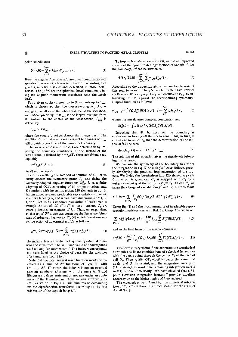
3.1.2 Article : “Shell structure in faceted metal clusters” (ref. [Pav93])
2Dans d’autres experiences ces deux metaux ont reveles une structure en couches quantiques, cf. ref. [Pel93]et ses citations.

3.1. AGREGATS METALLIQUES FACETTES 29
30 CHAPITRE 3. FACETTES ET DIFFRACTION
3.1. AGREGATS METALLIQUES FACETTES 31

32 CHAPITRE 3. FACETTES ET DIFFRACTION

3.1. AGREGATS METALLIQUES FACETTES 33
34 CHAPITRE 3. FACETTES ET DIFFRACTION

3.1. AGREGATS METALLIQUES FACETTES 35
36 CHAPITRE 3. FACETTES ET DIFFRACTION

3.1. AGREGATS METALLIQUES FACETTES 37

38 CHAPITRE 3. FACETTES ET DIFFRACTION
3.2. DEVELOPPEMENT DE WEYL EN PRESENCE DE SYMETRIES DISCRETES 39
3.2 Developpement de Weyl en presence de symetries discretes
L’etude du spectre du laplacien dans l’icosaedre (article supra) a motive une etude du termede Thomas-Fermi (cf. sa definition dans le chapitre 2) dans un billard en presence de symetriesdiscretes [Pav94]. En effet, le bon accord avec la formule de Thomas-Fermi (dans les billardson parle plutot de developpement de Weyl) projetee sur les representations irreductibles dugroupe de symetrie est un test important du calcul numerique des niveaux. En outre, si l’ons’interesse aux proprietes statistiques d’un spectre – comme c’est souvent le cas dans le domainedu chaos quantique – il faut utiliser le developpement de Weyl pour “deplier” le spectre etramener l’espacement entre niveaux a une valeur constante (cette procedure est decrite parexemple dans [Boh89]). Comme les statistiques spectrales n’ont de sens qu’etudiees separementpour chaque representation du groupe de symetrie, il est necessaire, pour le “depliage”, deconnaıtre le developpement de Weyl projete sur chaque representation. Cette projection estrendue difficile dans l’icosaedre, car son groupe de symetrie est tres riche et il n’est pas possibled’obtenir geometriquement sur un domaine elementaire de l’icosaedre les conditions de bordcorrespondant a chaque representation du groupe.
Dans la ref. [Pav94] on a obtenu un developpement de Weyl projete sur les differentesrepresentations irreductibles d’un groupe discret quelconque en utilisant seulement l’ingredientde la table des caracteres du groupe et les proprietes geometriques (telles la surface, le perimetreetc . . .) de sous-parties du billard invariantes sous une transformation du groupe. Un resultatinteressant de cette etude – qui semble-t-il n’avait jamais ete souligne jusqu’alors – est qu’a
l’ordre dominant, si l’on appelle ρTF (E) le terme de Thomas-Fermi et ρ(α)TF (E) sa projection sur
une representation irreductible (α) du groupe de symetrie G, on a
ρ(α)TF (E) =
(dα)2
|G| ρTF (E) + . . . , (3.2)
ou dα est la dimension de la representation (i.e. la degenerescence des niveaux) et |G| le nombred’elements du groupe (suppose discret). Le coefficient (dα)2 est surprenant : si par exemple ungroupe de symetrie correspond a des niveaux degeneres 5 fois et 1 fois, les etats 5 fois degeneresapparaissent 25 fois plus souvent dans le spectre. Dans ce coefficient 25, un facteur 5 est trivial,il correspond a la degenerescence des niveaux de la representation consideree ; mais le facteur5 restant est surprenant : il signifie qu’en tirant au hasard dans le spectre on a environ 5 foisplus de chances d’obtenir un niveau 5 fois degenere qu’un niveau non degenere !
3.2.1 Article : “Discrete symmetries in the Weyl expansion for quantumbilliards” (ref. [Pav94])

40 CHAPITRE 3. FACETTES ET DIFFRACTION
3.2. DEVELOPPEMENT DE WEYL EN PRESENCE DE SYMETRIES DISCRETES 41
42 CHAPITRE 3. FACETTES ET DIFFRACTION
3.2. DEVELOPPEMENT DE WEYL EN PRESENCE DE SYMETRIES DISCRETES 43

44 CHAPITRE 3. FACETTES ET DIFFRACTION
3.2. DEVELOPPEMENT DE WEYL EN PRESENCE DE SYMETRIES DISCRETES 45

46 CHAPITRE 3. FACETTES ET DIFFRACTION
3.3. DIFFRACTION 47
3.3 Diffraction
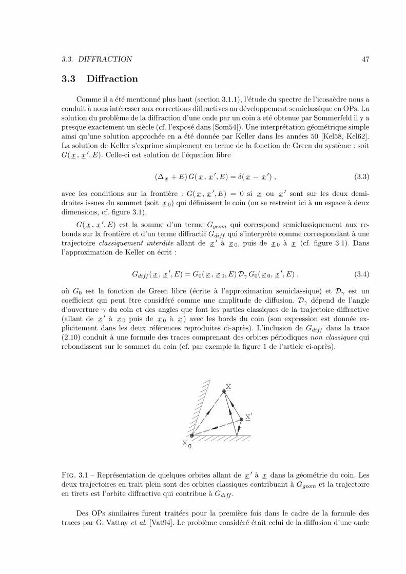
Comme il a ete mentionne plus haut (section 3.1.1), l’etude du spectre de l’icosaedre nous aconduit a nous interesser aux corrections diffractives au developpement semiclassique en OPs. Lasolution du probleme de la diffraction d’une onde par un coin a ete obtenue par Sommerfeld il y apresque exactement un siecle (cf. l’expose dans [Som54]). Une interpretation geometrique simpleainsi qu’une solution approchee en a ete donnee par Keller dans les annees 50 [Kel58, Kel62].La solution de Keller s’exprime simplement en terme de la fonction de Green du systeme : soitG(x , x ′, E). Celle-ci est solution de l’equation libre
(∆x + E)G(x , x ′, E) = δ(x − x ′) , (3.3)
avec les conditions sur la frontiere : G(x , x ′, E) = 0 si x ou x ′ sont sur les deux demi-droites issues du sommet (soit x 0) qui definissent le coin (on se restreint ici a un espace a deuxdimensions, cf. figure 3.1).
G(x , x ′, E) est la somme d’un terme Ggeom qui correspond semiclassiquement aux re-bonds sur la frontiere et d’un terme diffractif Gdiff qui s’interprete comme correspondant a unetrajectoire classiquement interdite allant de x ′ a x 0, puis de x 0 a x (cf. figure 3.1). Dansl’approximation de Keller on ecrit :
Gdiff (x , x ′, E) = G0(x , x 0, E)Dγ G0(x 0, x′, E) , (3.4)
ou G0 est la fonction de Green libre (ecrite a l’approximation semiclassique) et Dγ est uncoefficient qui peut etre considere comme une amplitude de diffusion. Dγ depend de l’angled’ouverture γ du coin et des angles que font les parties classiques de la trajectoire diffractive(allant de x ′ a x 0 puis de x 0 a x ) avec les bords du coin (son expression est donnee ex-plicitement dans les deux references reproduites ci-apres). L’inclusion de Gdiff dans la trace(2.10) conduit a une formule des traces comprenant des orbites periodiques non classiques quirebondissent sur le sommet du coin (cf. par exemple la figure 1 de l’article ci-apres).
Fig. 3.1 – Representation de quelques orbites allant de x ′ a x dans la geometrie du coin. Lesdeux trajectoires en trait plein sont des orbites classiques contribuant a Ggeom et la trajectoireen tirets est l’orbite diffractive qui contribue a Gdiff .
Des OPs similaires furent traitees pour la premiere fois dans le cadre de la formule destraces par G. Vattay et al. [Vat94]. Le probleme considere etait celui de la diffusion d’une onde

48 CHAPITRE 3. FACETTES ET DIFFRACTION
sur un systeme de disques. Les orbites periodiques diffractives sont alors des “orbites rampantes”(creeping orbits) dont un exemple est reproduit sur la figure 3.2.
Fig. 3.2 – Une orbite periodique diffractive rampant autour de deux disques.
Les orbites rampantes correspondent a des corrections exponentiellement faibles en com-paraison de la contribution dominante des OPs classiques. Le facteur d’attenuation exponentielest schematiquement de la forme exp{−Cste Lc (k/R2)1/3} ou Lc est la longueur de reptation lelong du disque et R le rayon du disque.
En revanche, dans le cas de la diffraction par un coin, la correction diffractive est algebriqueet non exponentielle. Cela se voit clairement sur la formule (3.4) : G0(x , x 0, E) etant de la formeCste exp{ik|x − x 0|}/
√
k|x − x 0|, et l’approximation de Keller pour Gdiff comportant deuxtermes G0, elle conduit dans la formule des traces a une correction d’ordre 1/
√k par rapport
au terme dominant (qui ne comprend lui qu’un seul terme G0).
Le cas d’OPs diffractives apparaissant lors de la diffraction par un coin a ete traite pour lapremiere fois dans la ref. [Pav95b] qui est reproduite ci-apres.
3.3.1 Article : “Diffractive orbits in quantum billiards” (ref. [Pav95b])
3.3. DIFFRACTION 49
VOLUME 75, NUMBER 1 P HY S I CA L REV I EW LE T T ER S 3 JULY 1995
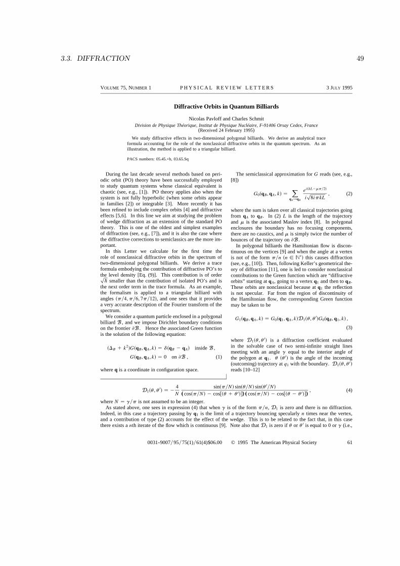
Diffractive Orbits in Quantum Billiards
Nicolas Pavloff and Charles SchmitDivision de Physique Théorique, Institut de Physique Nucléaire, F-91406 Orsay Cedex, France
(Received 24 February 1995)
We study diffractive effects in two-dimensional polygonal billiards. We derive an analytical traceformula accounting for the role of the nonclassical diffractive orbits in the quantum spectrum. As anillustration, the method is applied to a triangular billiard.
PACS numbers: 05.45.+b, 03.65.Sq
During the last decade several methods based on peri-odic orbit (PO) theory have been successfully employedto study quantum systems whose classical equivalent ischaotic (see, e.g., [1]). PO theory applies also when thesystem is not fully hyperbolic (when some orbits appearin families [2]) or integrable [3]. More recently it hasbeen refined to include complex orbits [4] and diffractiveeffects [5,6]. In this line we aim at studying the problemof wedge diffraction as an extension of the standard POtheory. This is one of the oldest and simplest examplesof diffraction (see, e.g., [7]), and it is also the case wherethe diffractive corrections to semiclassics are the more im-portant.In this Letter we calculate for the first time the
role of nonclassical diffractive orbits in the spectrum oftwo-dimensional polygonal billiards. We derive a traceformula embodying the contribution of diffractive PO’s tothe level density [Eq. (9)]. This contribution is of orderp
h smaller than the contribution of isolated PO’s and isthe next order term in the trace formula. As an example,the formalism is applied to a triangular billiard withangles spy4, py6, 7py12d, and one sees that it providesa very accurate description of the Fourier transform of thespectrum.We consider a quantum particle enclosed in a polygonal
billiard B , and we impose Dirichlet boundary conditionson the frontier ≠B . Hence the associated Green functionis the solution of the following equation:
sDB 1 k2dGsqB, qA, kd dsqB 2 qAd inside B ,
GsqB, qA, kd 0 on ≠B , (1)
where q is a coordinate in configuration space.
The semiclassical approximation for G reads (see, e.g.,[8])
G0sqB, qA, kd
X
qA!qB
eiskL2mpy2d
ip
8ipkL, (2)
where the sum is taken over all classical trajectories goingfrom qA to qB. In (2) L is the length of the trajectoryand m is the associated Maslov index [8]. In polygonalenclosures the boundary has no focusing components,there are no caustics, and m is simply twice the number ofbounces of the trajectory on ≠B .In polygonal billiards the Hamiltonian flow is discon-tinuous on the vertices [9] and when the angle at a vertexis not of the form pyn sn [ ,
pd this causes diffraction(see, e.g., [10]). Then, following Keller’s geometrical the-ory of diffraction [11], one is led to consider nonclassicalcontributions to the Green function which are “diffractiveorbits” starting at qA, going to a vertex q1 and then to qB.These orbits are nonclassical because at q1 the reflectionis not specular. Far from the region of discontinuity ofthe Hamiltonian flow, the corresponding Green functionmay be taken to be
G1sqB, qA, kd G0sq1, qA, kdD1su, u0dG0sqB, q1, kd ,
(3)
where D1su, u0d is a diffraction coefficient evaluatedin the solvable case of two semi-infinite straight linesmeeting with an angle g equal to the interior angle ofthe polygon at q1. u su0d is the angle of the incoming(outcoming) trajectory at q1 with the boundary. D1su, u0dreads [10–12]
D1su, u0d 24
N
sinspyNd sinsuyNd sinsu0yNd
sss cosspyNd 2 cosfsu 1 u0dgddd sss cosspyNd 2 cosfsu 2 u0dgddd, (4)
where N gyp is not assumed to be an integer.As stated above, one sees in expression (4) that when g is of the form pyn, D1 is zero and there is no diffraction.
Indeed, in this case a trajectory passing by q1 is the limit of a trajectory bouncing specularly n times near the vertex,and a contribution of type (2) accounts for the effect of the wedge. This is to be related to the fact that, in this casethere exists a nth iterate of the flow which is continuous [9]. Note also thatD1 is zero if u or u0 is equal to 0 or g (i.e.,
0031-9007y95y75(1)y61(4)$06.00 © 1995 The American Physical Society 61

50 CHAPITRE 3. FACETTES ET DIFFRACTION
VOLUME 75, NUMBER 1 P HY S I CA L REV I EW LE T T ER S 3 JULY 1995
in the case of a diffractive trajectory having a segmentlying on a face).For an orbit with several diffractive reflections at points
q1, . . . , qn , formula (3) becomes
GnsqB, qA, kd G0sq1, qA, kd
3
(n21Y
j1
DjG0sqj11, qj, kd
)
Dn
3 G0sqB, qn , kd , (5)
whereDj is the diffraction coefficient at point qj as givenby (4).In (2), (3), and (5) the indices 0, 1, or n of the Green
function recall that diffractive effects are subdominant (bya factor of order k2ny2). There might be less severenonanalyticities on the boundary leading to higher-orderdiffractive corrections. Note also that we are using here asimple approximation for the Green function which is notvalid when the angles u and u0 at an edge are such thatthe diffractive orbit is close to being real; in this case thecoefficientD1su, u0d diverges. This occurs in the vicinityof the line of discontinuity of the Hamiltonian flow. Inorder to have a formula valid in all regions of space, oneshould use a uniform approximation such as first providedby Pauli [12] and whose general form is given in [10] (seealso [13]).The level density rskd is then obtained from the Green
function by the usual formula:
rskd 22k
pIm
Z
Bd2q Gsq, q, kd . (6)
rskd can be separated in a smooth function of k, rskdplus an oscillating part rskd. The zero-length trajectoriesin (6) contribute to r and will not be considered in detailhere (see [14]). When G is replaced by its semiclassi-cal approximation (2), a stationary phase evaluation of (6)corresponds in considering only the contribution of clas-sical PO’s to r. When diffractive orbits such as (5) aretaken into account, one is led to consider also “diffractivePO’s,” [5] which are PO’s with one or several diffractivereflections (examples of such orbits are given in Fig. 1).Let us consider first the contribution of classical PO’s.
In a polygonal enclosure there is a drastic difference be-tween PO’s with even and odd number of bounces. Thelatter ones do not remain periodic when a point of reflec-tion is translated along a face (they period double intoa PO with twice as many bounces). This can be under-stood by remembering that, for the phase-space coordi-nates transverse to the direction of an orbit, a bounce ona straight segment leads to an inversion. On the otherhand, PO’s with an even number of bounces form fam-ilies which correspond to local translation parallel to thefaces of the polygon. They are neutral (or direct para-bolic; see [8]) PO’s to which the usual trace formula doesnot apply; we use a generalization of Gutzwiller’s theory
FIG. 1. The shortest classical and diffractive PO’s in thetriangle (py4, py6, 7py12). All these orbits are self-retracing.For diffractive PO’s the diffraction point is marked with a blackspot. Orbits 6 and 10 form families, 5 and 7 are isolated. Thelengths are given in units of the height of the triangle.
which is valid for the case of degenerate PO’s [2]. Wequote here the result and leave detailed discussion for thefuture [13]. A family of orbits contributes to rskd as
rskd √s
kL
2rp3d' cosskrL 2 py4d . (7)
Equation (7) is written for the general case of the rthiterate of a primitive orbit of length L sr [ ,
pd. d' isthe length occupied by the family perpendicular to theorbit’s direction. It is equal to d cosf, where d is thelength occupied by the family on a face and f is the anglebetween the direction of the orbit and the normal to thisface.For an isolated PO with an odd number of bounces, onehas the following contribution:
rskd √ 2L
2pcosskrLd . (8)
Formula (8) holds when the number of repetitions isodd. When r is even, the rth iterate of an isolated orbitleads to a family, and formula (7) applies.The derivation of the contribution of a diffractive POis patterned on what is done in Gutzwiller’s trace formulafor an isolated PO. The length of a closed diffractiveorbit in the vicinity of the diffractive PO is expanded upto second order, and the trace of the Green function isevaluated by a stationary phase approximation. The finalcontribution of a generic diffractive PO with n diffractivereflections to the oscillating part of the level density reads:
rskd √ L
p
(nY
j1
Djp
8pkLj
)
cosskL 2 mpy2 2 3npy4d .
(9)
62
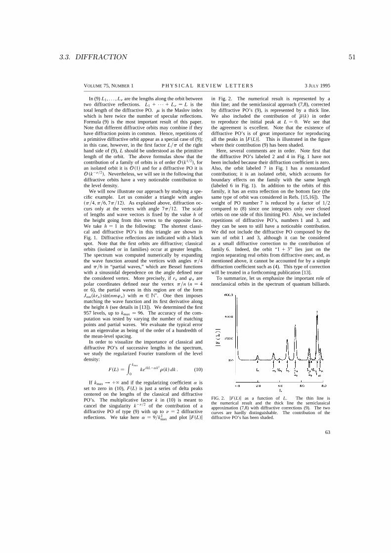
3.3. DIFFRACTION 51
VOLUME 75, NUMBER 1 P HY S I CA L REV I EW LE T T ER S 3 JULY 1995
In (9) L1, . . . , Ln are the lengths along the orbit betweentwo diffractive reflections. L1 1 · · · 1 Ln L is thetotal length of the diffractive PO. m is the Maslov indexwhich is here twice the number of specular reflections.Formula (9) is the most important result of this paper.Note that different diffractive orbits may combine if theyhave diffraction points in common. Hence, repetitions ofa primitive diffractive orbit appear as a special case of (9);in this case, however, in the first factor Lyp of the righthand side of (9), L should be understood as the primitivelength of the orbit. The above formulas show that thecontribution of a family of orbits is of order O sk1y2d, foran isolated orbit it is O s1d and for a diffractive PO it isO sk2ny2d. Nevertheless, we will see in the following thatdiffractive orbits have a very noticeable contribution tothe level density.We will now illustrate our approach by studying a spe-
cific example. Let us consider a triangle with anglesspy4, py6, 7py12d. As explained above, diffraction oc-curs only at the vertex with angle 7py12. The scaleof lengths and wave vectors is fixed by the value h ofthe height going from this vertex to the opposite face.We take h 1 in the following: The shortest classi-cal and diffractive PO’s in this triangle are shown inFig. 1. Diffractive reflections are indicated with a blackspot. Note that the first orbits are diffractive; classicalorbits (isolated or in families) occur at greater lengths.The spectrum was computed numerically by expandingthe wave function around the vertices with angles py4
and py6 in “partial waves,” which are Bessel functionswith a sinusoidal dependence on the angle defined nearthe considered vertex. More precisely, if rn and wn arepolar coordinates defined near the vertex pyn sn 4
or 6), the partial waves in this region are of the formJnmskrnd sinsnmwnd with m [ ,
p. One then imposesmatching the wave function and its first derivative alongthe height h (see details in [13]). We determined the first957 levels, up to kmax . 96. The accuracy of the com-putation was tested by varying the number of matchingpoints and partial waves. We evaluate the typical erroron an eigenvalue as being of the order of a hundredth ofthe mean-level spacing.In order to visualize the importance of classical and
diffractive PO’s of successive lengths in the spectrum,we study the regularized Fourier transform of the leveldensity:
FsLd
Z kmax
0
keikL2ak2
rskd dk . (10)
If kmax ! 1` and if the regularizing coefficient a isset to zero in (10), FsLd is just a series of delta peakscentered on the lengths of the classical and diffractivePO’s. The multiplicative factor k in (10) is meant tocancel the singularity k2ny2 of the contribution of adiffractive PO of type (9) with up to n 2 diffractivereflections. We take here a 9yk2
max and plot jFsLdj
in Fig. 2. The numerical result is represented by athin line; and the semiclassical approach (7,8), correctedby diffractive PO’s (9), is represented by a thick line.We also included the contribution of rskd in orderto reproduce the initial peak at L 0. We see thatthe agreement is excellent. Note that the existence ofdiffractive PO’s is of great importance for reproducingall the peaks in jFsLdj. This is illustrated in the figurewhere their contribution (9) has been shaded.Here, several comments are in order. Note first thatthe diffractive PO’s labeled 2 and 4 in Fig. 1 have notbeen included because their diffraction coefficient is zero.Also, the orbit labeled 7 in Fig. 1 has a nonstandardcontribution; it is an isolated orbit, which accounts forboundary effects on the family with the same length(labeled 6 in Fig. 1). In addition to the orbits of thisfamily, it has an extra reflection on the bottom face (thesame type of orbit was considered in Refs. [15,16]). Theweight of PO number 7 is reduced by a factor of 1y2compared to (8) since one integrates only over closedorbits on one side of this limiting PO. Also, we includedrepetitions of diffractive PO’s, numbers 1 and 3, andthey can be seen to still have a noticeable contribution.We did not include the diffractive PO composed by thesum of orbit 1 and 3, although it can be consideredas a small diffractive correction to the contribution offamily 6. Indeed, the orbit “1 1 3” lies just on theregion separating real orbits from diffractive ones; and, asmentioned above, it cannot be accounted for by a simplediffraction coefficient such as (4). This type of correctionwill be treated in a forthcoming publication [13].To summarize, let us emphasize the important role ofnonclassical orbits in the spectrum of quantum billiards.
FIG. 2. jFsLdj as a function of L. The thin line isthe numerical result and the thick line the semiclassicalapproximation (7,8) with diffractive corrections (9). The twocurves are hardly distinguishable. The contribution of thediffractive PO’s has been shaded.
63

52 CHAPITRE 3. FACETTES ET DIFFRACTION
VOLUME 75, NUMBER 1 P HY S I CA L REV I EW LE T T ER S 3 JULY 1995
The existence of these orbits affects qualitatively theFourier transform of the spectrum. The above exampleis only one among others where the discontinuity ofthe classical dynamics is linked to strong diffractivecorrections to semiclassics. It was argued in [17] that thesame type of corrections should be taken into account forthe three-dimensional icosahedral billiard. We also expectdiffractive effects—of the same order as those describedhere—in more general billiards with cusps (nonpolygonalor with an additional external field); in these cases asimple generalization of formula (9) accounts for the roleof diffractive PO’s. Finally, we note that the presentwork illustrates that semiclassical methods provide a veryappealing tool which, when corrected with tunneling ordiffractive effects, allows one to describe accurately thesolution of partial differential equations using simplegeometrical methods.It is a pleasure to thank E. Bogomolny and D. Ullmo
for fruitful discussions. Division de Physique Théoriqueis a Unité de Recherche des Universités de Paris XI etParis VI associée au CNRS.
[1] For a review see Chaos and Quantum Mechanics, editedby M. J. Giannoni, A. Voros, and J. Zinn-Justin, lesHouches Summer School Lectures LII (North-Holland,Amsterdam, 1989), and also Chaos 2, 1–158 (1992).
[2] S. C. Creagh and R. G. Littlejohn, Phys. Rev. A 44, 836(1991); J. Phys. A 25, 1643 (1992).
[3] M.V. Berry and M. Tabor, Proc. R. Soc. London, Sect. A349, 101 (1976); J. Phys. A 10, 371 (1977).
[4] J.M. Robbins, S. C. Creagh, and R. G. Littlejohn, Phys.Rev. A 39, 2838 (1989); M. Kus, F. Haake, andD. Delande, Phys. Rev. Lett. 71, 2167 (1993); P. Leboeufand A. Mouchet, Phys. Rev. Lett. 73, 1360 (1994).
[5] G. Vattay, A. Wirzba, and P. E. Rosenqvist, Phys. Rev.Lett. 73, 2304 (1994).
[6] N. D. Whelan, Phys. Rev. E 51, 3778 (1995).[7] A. Sommerfeld, Optics (Academic, New York, 1954).[8] M. C. Gutzwiller, Chaos in Classical and Quantum Me-chanics (Springer-Verlag, New York, 1990).
[9] T. Dagaeff and C. Rouvinez, Physica (Amsterdam) 67D,166 (1993).
[10] G. L. James, Geometrical Theory of Diffraction for Elec-tromagnetic Waves (Peregrinus, Stevenage, 1976).
[11] J. B. Keller, J. Opt. Soc. Am. 52, 116 (1962).[12] W. Pauli, Phys. Rev. 54, 924 (1938).[13] N. Pavloff and C. Schmit (to be published).[14] H. Baltes and E.R. Hilf, Spectra of Finite Systems
(Bibliographisches Institute, Mannheim, 1976).[15] B. Lauritzen, Phys. Rev. A 43, 603 (1991).[16] M. Sieber, U. Smilansky, S. C. Creagh, and R. G. Little-
john, J. Phys. A 26, 6217 (1993).[17] N. Pavloff and S. C. Creagh, Phys. Rev. B 48, 18 164
(1993).
64

3.3. DIFFRACTION 53
3.3.2 Approximation uniforme
L’approximation de Keller (3.4) du resultat exact de Sommerfeld n’est pas uniformementvalable. Le coefficient Dγ diverge lorsqu’une orbite diffractive tend a devenir une orbite au-torisee par la mecanique classique (cf. la figure 3.3). Cela se comprend intuitivement d’apresla forme de l’expression approchee (3.4) : lorsque la trajectoire diffractive tend a devenir unetrajectoire classique autorisee, Gdiff (x , x ′, E) doit tendre vers G0(x , x
′, E), c’est-a-dire doitdevenir d’ordre O(k−1/2) alors qu’il est d’ordre O(k−1). Dans ce regime la formule cesse doncd’etre valable.
Fig. 3.3 – Une orbite diffractive allant de x ′ a x (en tirets). Dans la formule (3.4), Dγ divergelorsque x se rapproche de la droite pointillee (que l’on appelle la frontiere optique), i.e. lorsquela trajectoire diffractive se rapproche d’une trajectoire reelle.
Dans la reference reproduite ci-apres, nous avons obtenu une formule des traces traitantpour la premiere fois la contribution des orbites diffractives de maniere uniforme ; c’est-a-direque la formule obtenue decrit aussi bien des orbites “tres diffractives” (situees loin de la zoneou une orbite diffractive devient reelle et qui est appelee frontiere optique, cf. figure 3.3) que lesorbites devenues reelles apres avoir traverse la frontiere optique (lors d’une modification ad hoc
de la forme du billard par exemple). On obtient alors une formule des traces interpolant entrela formule usuelle de Gutzwiller et les formules utilisant des approximations a la Keller.
Le calcul repose sur une analyse detaillee de la solution de Sommerfeld (s’inspirant d’uneapproximation obtenue pour la premiere fois par Pauli [Pau38]) et des differentes contributionsa la trace (2.10) au voisinage de la frontiere optique. Le cas de la diffraction par un coin estjusqu’a present le seul qui ait permis un traitement uniforme dans la formule des traces et iln’existe pas d’approximation uniforme dans le cas des trajectoires rampantes (seul un traitementlocal au voisinage de la frontiere optique a ete obtenu dans la ref. [Pri97]).
3.3.3 Article : “Uniform approximation for diffractive contributions to thetrace formula in billiard systems” (ref. [Sie97])

54 CHAPITRE 3. FACETTES ET DIFFRACTION
Uniform approximation for diffractive contributions to the trace formula in billiard systems
Martin Sieber, 1,2 Nicolas Pavloff, 1 and Charles Schmit 11Division de Physique Theorique, Institut de Physique Nucleaire, F-91406 Orsay Cedex, France
2Abteilung Theoretische Physik, Universitat Ulm, D-89069 Ulm, Germany~Received 23 August 1996!
We derive contributions to the trace formula for the spectral density accounting for the role of diffractiveorbits in two-dimensional billiard systems with corners. This is achieved by using the exact Sommerfeldsolution for the Green function of a wedge. We obtain a uniformly valid formula for single-diffractive orbitswhich interpolates between formerly separate approaches ~the geometrical theory of diffraction and Gutzwill-er’s trace formula!. It yields excellent numerical agreement with exact quantum results, also in cases whereother methods fail. @S1063-651X~97!12902-6#
PACS number~s!: 05.45.1b, 03.40.Kf, 03.65.Sq
I. INTRODUCTION
Two-dimensional classical billiards became popular asmodel systems exhibiting a rich variety of dynamical behav-ior, ranging from integrable to fully chaotic. Their quantumcounterparts attracted much interest starting in the 1980s,from both the point of view of random matrix theory and thesemiclassical periodic orbit theory. In the latter approach oneuses trace formulas of the type first derived by Gutzwiller @1#and Balian and Bloch @2,3#.
During the last two years, following the route opened byRef. @4#, a number of studies ~see Refs. @5–8#! have concen-trated on additional contributions to the trace formula linkedto diffractive effects near regions where the classical Hamil-tonian flow is discontinuous. These zones of discontinuityare known as ‘‘optical boundaries’’ in the literature. Theylead to contributions from nonclassical ~so-called diffractive!orbits hitting a corner of the billiard or creeping around asmooth boundary.
Apart from the noticeable exception of Ref. @7#, all thework quoted above is based on Keller’s ‘‘geometrical theoryof diffraction’’ ~GTD; see, e.g., @9#!, i.e., on an extension ofgeometrical optics which accounts for diffractive effects.Keller’s approach fails when the diffractive trajectory is veryclose to an optical boundary, or equivalently when the dif-fractive orbit is close to become an allowed classical trajec-tory ~this will be clarified in the text of the paper!. In thepresent work we use a uniform approximation for the Greenfunction which does not have this drawback. This allows usto derive relatively simple formulas which are uniformlyvalid. The method is applied to billiards whose boundary hasa slope discontinuity, and thus we restrict our study to wedgediffraction effects. To our knowledge there does not yet exista uniformly valid formula for the contributions of creepingorbits ~despite the progress made in Ref. @7#!.
The theory of uniform approximations for wedge diffrac-tion has a long history which begins with a famous paper byPauli @10#. In the late 1960s and in the 1970s the problemwas studied in detail. Much literature was devoted to severaltypes of approaches remedying the deficiency of the geo-metrical theory of diffraction. The approach most widelyused is known as ‘‘uniform asymptotic theory’’ and was de-veloped in Refs. @11–14#. Here we have chosen a technique
more closely related to the original work of Sommerfeld andPauli. It relies on an extension of the method of steepestdescent due to Pauli, which was carefully studieed on a gen-eral setting by Clemmow @15#. The method, due to Kouy-oumjian and Pathak, is known as ‘‘uniform theory of diffrac-tion’’ and is exposed in Refs. @16# and @17#. Note that weapply the uniform approximation only to orbits with a singlediffractive point. The treatment of multiple wedge diffractionis increasingly more involved, as can be seen in work ondouble diffraction by half-planes ~see Refs. @18–20#! orwedges @21#. To our knowledge, there does not exist to datea general uniform approximation for multiple wedge diffrac-tion.
The paper is organized as follows. In Sec. II we recall theexact solution of the infinite wedge problem, derive a uni-form approximation for the Green function, and compare itwith the result obtained from GTD. In Sec. III we use theGreen function obtained previously to derive contributions tothe trace formula which are uniformly valid. Readers mostlyinterested in the final result can skip this part and go directlyto Sec. IV, where we discuss the previously obtained formulaand several of its limits. In particular, we show that thisformula has the appealing feature of interpolating betweenthe semiclassical results of periodic orbit theory and the for-mulas obtained in Refs. @4,6,8#. Section V contains numeri-cal applications for several simple billiard systems. In somecases GTD gives reasonable results, but in other cases theuniform approximation has to be used in order to describethe Fourier transform of the spectral density correctly. Fi-nally we discuss our results and possible extensions in Sec.VI.
II. GREEN FUNCTION OF AN INFINITE WEDGE
In this section we consider an infinite wedge of interiorangle g (gP#0,2p]) with Dirichlet boundary conditions,and derive several approximations for the Green function.
A. Exact result
The exact solution of the problem was first given by Som-merfeld for a wedge with g52p ~a half line! and an incidentplane wave; see @22#. The solution of the general problem is
PHYSICAL REVIEW E MARCH 1997VOLUME 55, NUMBER 3
551063-651X/97/55~3!/2279~21!/$10.00 2279 © 1997 The American Physical Society

3.3. DIFFRACTION 55
easily inferred from his approach, a complete treatment isgiven for instance by Carslaw in Refs. @23,24#. Here, forcompleteness, we recall some properties of the solution.
The Green function Gg(rW ,rW8,E) of the problem in dimen-sionless units is a solution of
~DrW1E !Gg~rW ,rW8,E !5d~rW2rW8!,
~1!
Gg[0 if rW or rW8 are on the boundary.
Choosing a system of coordinates with the origin at thevertex and the polar axis along one of the boundaries suchthat u and u8 are in @0,g# @see Fig. 2~a!#, one can write thefollowing integral representation for the exact solution:
Gg~rW ,rW8,E !5gg~r ,r8,u82u !2gg~r ,r8,u81u !, ~2!
with
gg~r ,r8,fs!
52
i
8pNEA1BdzH0
~1 !~kAr21r8222rr8cosz !
12exp„2i~z2fs!/N….
~3!
In Eq. ~3! and in the following the angles u and u8 alwaysappear in the combination u86u , and we will denotefs5u82su (s561). Other quantities appearing in Eq.~3! are N5g/p , k5AE , which is the modulus of the wavevector, H0
(1) , which is the Hankel function of the first kind~see @25#!, and A and B , which are the contours in the com-plex plane drawn in Fig. 1. In this figure one can further seethe poles of the integrand corresponding to (z2fs)/N52np ~with nPZ) — they appear as black points — andbranch cuts linked to the square root argument of H0
(1) . Theshaded areas are zones where the integrand increases withoutlimit when one goes away from the real axis @this is easilychecked by using the leading asymptotic term ~7! of the Han-kel function#. The integration contour is quite arbitrary aslong as it goes to infinity in the indicated unshaded regions.
This solution was obtained by a generalization of themethod of images. This generalization expresses the solution
in terms of functions that are defined on a Riemann surfacewith p sheets if the opening angle is g5pp/q ~with p andq coprime!, or an infinite number of sheets when g is anirrational multiple of p ~see Refs. @22–24#!.
Essentially, gg is a superposition of free Green functions~with complex angles z). Considered as a function of fs , ithas periodicity 2pN52g , and this ensures that the Greenfunction ~2! satisfies the boundary conditions for u50 andg . By moving the contours A and B toward the real line zP@2p ,p# , and taking into account the poles of the inte-grand, one obtains
gg~r ,r8,fs!52
i
4(n8H0
~1 !
3~kAr21r8222rr8cos~fs22ng !!
1hg~r ,r8,fs!, ~4!
where, after a change of variable, hg can be written in theform
hg~r ,r8,fs!
5
sin~p/N !
8pN E2i`
1i`
dzH0
~1 !~kAr21r8212rr8cosz !
cos@~z1fs!/N#2cos~p/N !.
~5!
The first term on the right-hand side of Eq. ~4! contains thecontributions of those poles of the integrand of Eq. ~3! whichlie between 2p and p; the prime indicates that the summa-tion is restricted to values of n such that 2p<fs22ng<p . If fs is exactly equal to 6p12ng , then the corre-sponding contribution to the summation has to be divided by2. In Eq. ~5! the contour can be modified as long as no poleof the integrand is crossed. A further requirement is that thepart of the contour extending to infinity has to start at2i` , with a real part in @0,p@ and to extend to i` with areal part in ]2p ,0].
The discrete summation in Eq. ~4! can be interpreted asarising from allowed classical trajectories. For instance, thecase f15u82u and n50 makes a contribution2(i/4)H0
(1)(kurW2rW8u), and corresponds to the free propaga-
tion from rW8 to rW . The other terms in the summation corre-spond to trajectories experiencing specular reflections on theboundaries @this is illustrated in Fig. 2~b!#. If s51
FIG. 1. Integration contour in the complex plane for formula~3!. The shaded areas are zones where the integrand diverges whengoing away from the real axis. The black points are poles andbranch points of the integrand. The thick lines are branch cuts.
FIG. 2. ~a! displays the notations used in the text. ~b! shows twoclassical trajectories ~solid lines! and the diffractive orbit going
from rW8 to rW ~dashed line!.
2280 55MARTIN SIEBER, NICOLAS PAVLOFF, AND CHARLES SCHMIT

56 CHAPITRE 3. FACETTES ET DIFFRACTION
(s521) the orbit has an even ~odd! number of reflections.These orbits correspond to successive applications of themethod of images and their contribution is known as thegeometrical term in the literature. When inserted back intoEq. ~2! they give a term which will be denotedGgeo(rW ,rW8,E) in the following.
If the angle g is of the form p/p (pPN*) thensin(p/N)50 and the term hg(r ,r8,fs) is zero: the geometri-cal term alone is enough to fulfill the boundary conditions.This is due to the fact that in this case the Green function canbe determined by the method of images. If gÞp/p , thenhg corresponds to the contribution from diffraction. Hencethe total Green function can be written as a sum of a geo-metrical plus a diffractive term:
Gg~rW ,rW8,E !5Ggeo~rW ,rW8,E !1Gdiff~rW ,rW8,E !,
with
Gdiff~rW ,rW8,E !5hg~r ,r8,u82u !2hg~r ,r8,u81u !. ~6!
B. Geometrical theory of diffraction
We now derive a simple approximation for Gdiff . We firstreplace the Hankel function by its asymptotic form for largearguments ~see @25#!,
H0~1 !~z !'S 2
pz D1/2
e iz2ip/4 when uzu@1. ~7!
The same approximation is also used in all the following forthe geometrical and diffractive Green functions, i.e., for allthe terms of Eqs. ~4! and ~5!, the assumption being that thedistances measured along the paths ~classical or diffractive!going from rW8 to rW are large compared to the wavelengthl52p/k . Then, in the integral defining hg , there is a saddlepoint of the exponent at z50, and a steepest descent ap-proximation yields
hg~r ,r8,fs!'1
4pN
sin~p/N !
cos~fs /N !2cos~p/N !
e ik~r1r8!1ip/2
kArr8.
~8!
Incorporating this result into expression ~6! for Gdiff , oneobtains a formula which can be cast into the form
Gdiff~rW ,rW8,E !'Gsc~rW ,rW0 ,E !D~u ,u8!Gsc~rW0 ,rW8,E !, ~9!
with
D~u ,u8!5
2
Nsin
p
N F S cospN2cosu1u8
N D 21
2S cospN2cosu2u8
N D 21G52
4
N
sin~p/N !sin~u/N !sin~u8/N !
S cospN2cosu1u8
N D S cospN2cosu2u8
N D .~10!
In Eq. ~9! Gsc is the free Green function evaluated using Eq.
~7!, and rW0 is the point at the vertex @see Fig. 2~a!#. Expres-sions ~9! and ~10! give the diffractive part of the Green func-tion in the ‘‘geometrical theory of diffraction’’ ~see @9#!.They have the simple interpretation of being the contribution
of a ~nonclassical! diffractive trajectory going from rW8 to rW0and then from rW0 to rW @see Fig. 2~b!#. Using this approxima-tion one can derive a trace formula for the spectral densitywhich accounts for diffractive effects in the GTD approxi-mation ~see Refs. @4,6,8#!.
The quantity D(u ,u8) is known as the diffraction coeffi-cient. It is zero if u ~or u8) is equal to 0 or g , or if p/g is an
integer. It diverges on an optical boundary, i.e., if rW and rW8
are such that the diffractive orbit is the limit of a classicaltrajectory. This is illustrated by the simple case of diffractionby a sharp wedge (g.3p/2) in Fig. 3. In this case there aretwo optical boundaries represented by dashed lines. Theycorrespond to u5u81p ~i.e., f15u82u52p) andu5p2u8 ~i.e., f25u81u5p). In the terminology of geo-metrical optics, the first optical boundary separates the illu-minated and shadowed regions for direct rays when the point
rW8 is considered as a light source ~boundary between regionsII and III!, and the second optical boundary separates theilluminated and shadowed regions for rays that are reflectedon one side of the wedge ~boundary between regions I and
II!. If rW lies near one of the optical boundaries then the dif-fractive path is almost an allowed classical trajectory, and if
rW is moved onto an optical boundary then the diffractive pathcoincides in this limit with an allowed classical trajectory.
Looking in more detail at the origin of the divergence,one sees from Eq. ~8! that it occurs when there exits aninteger n such that fs56p12nNp . In this case there is apole z5fs7p22nNp50 in the integral representation ofthe diffractive part ~5! which is at the same position as thesaddle point z50 and thus the saddle point approximationbreaks down. More generally, the geometrical theory of dif-fraction is only valid if all poles are sufficiently far awayfrom the saddle point z50. This can be interpreted in termsof the physical trajectories in the system because, in Som-
FIG. 3. Optical boundaries ~dashed lines! for an initial point
rW8 in the case of diffraction by a sharp wedge (g.3p/2). Thetransition regions ~for r8510l) around the optical boundaries areshaded.
55 2281UNIFORM APPROXIMATION FOR DIFFRACTIVE . . .

3.3. DIFFRACTION 57
merfeld’s solution @Eqs. ~2! and ~3!#, the saddle point corre-sponds to the diffractive orbit, and the poles correspond togeometrical orbits.
C. A uniform approximation
As seen above, one has to refine the steepest descentevaluation of hg in the case when there is a pole of theintegrand near the saddle point z50. This was first done byPauli @10#, and here we present a slight modification of theoriginal procedure @16,17#. In a first step one can separatepoles which are possibly near one another by using the iden-tity
2sin~p/N !
cosS z1fs
N D2cos~p/N !
5
1
tanS z1fs1p
2N D2
1
tanS z1fs2p
2N D . ~11!
Hence hg in Eq. ~5! can be rewritten as
hg~r8,r ,fs!5ug ,1~r8,r ,fs!2ug ,2~r8,r ,fs!, ~12!
where
ug ,h~r ,r8,fs!
5
1
16pNE2i`
1i`
dzH0
~1 !~kAr21r8212rr8cosz !
tanS z1fs1hp
2N D ,
~13!
and h561 is a new index.If one denotes the nearest integer to (fs1hp)/(2g) by
ns ,h , then z52(fs1hp)12 ns ,hg is the pole of the inte-grand of Eq. ~13! which is nearest to the saddle point z50.Thanks to the separation ~12! the next pole in the integrandof Eq. ~13! is at distance 2g , and its effect can safely beneglected if g is not a small angle ~this will be assumed inthe following!. According to the method of Pauli one re-writes the integrand by multiplying the numerator and de-nominator by a function imitating the behavior of the origi-nal denominator but in which the z and fs parts areseparated. This procedure is not unique; it corresponds to aspecific choice of a uniform approximation, as will be dis-cussed below. The choice for the function ishA2sin(z/2)1as ,h , where as ,h is a measure of the separa-tion between the saddle point z50 and the nearest opticalboundary:
as ,h5A2cosS fs
22ns ,hg D
with
ns ,h5nint Ffs1hp
2g GPZ, ~14!
where nint denotes the nearest integer. Using the asymptoticformula ~7! for the Hankel function, one obtains
ug ,h~r ,r8,fs!
'e2ip/4
8gA2pkE
2i`
1i`
dze ikAr
21r8212rr8cosz
hA2sin~z/2!1as ,h
Fs ,h~z !,
~15!
where Fs ,h(z) is a smooth function at z50, even in thevicinity of an optical boundary @when as ,h→0, see Eq.~20!#:
Fs ,h~z !5
hA2sin~z/2!1as ,h
~r21r8212rr8cosz !1/4 tanS z1fs1hp
2N D .
Note that the integrands of Eqs. ~15! and ~13! both have thepole z52(fs1hp)12 ns ,hg next to the origin, as men-tioned above.
Now Eq. ~15! is evaluated along the steepest descent pathat z50 by a change of variable z5htA2exp(i3p/4), with tPR ~the factor hA2 is here for convenience!. The smooth,nonsingular part Fs ,h of the integrand is simply evaluated att50, and the phase of the exponential function and the de-nominator are expanded in the vicinity of the origin:
hA2sin~z/2!1as ,h5as ,h1te3ip/41O~ t3! ~16!
and
ikAr21r8212rr8cosz5ik~r1r8!2
krr8
r1r8t21O~ t3!.
~17!
Hence ug ,h is approximated by
ug ,h~r ,r8,fs!'e ik~r1r8!2ip/4
8gApk~r1r8!
as ,h
tanS fs1hp
2N D3E
2`
`
dtexp@2krr8t2/~r1r8!#
t2as ,h eip/4 .
~18!
After expansion ~16! of the denominator, the pole in Eq. ~18!is only approximately equal to the nearest pole in Eq. ~13!,but they coincide when the pole approaches the stationarypoint t50. As noted above, the choice of the uniform ap-proximation which leads to Eq. ~18! is not unique ~as dis-cussed by Clemmow, who calls it a ‘‘partial asymptotic ex-pansion’’; see @15#!. For example, another choice of auniform approximation can be obtained by making a changeof variable which transforms the exponent in Eq. ~15! suchthat it becomes an exact quadratic function, and multiply thedenominator and integrand by a function which is linear inthe variable. Then one obtains Eq. ~18! with a different defi-nition of as ,h which is expressed in terms of a ‘‘detour pa-rameter’’ such as used in the ‘‘uniform approximationtheory’’ ~see Refs. @11–14#!. In practical applications, how-
2282 55MARTIN SIEBER, NICOLAS PAVLOFF, AND CHARLES SCHMIT

58 CHAPITRE 3. FACETTES ET DIFFRACTION
ever, the differences between different uniform approxima-tions are small. We would like to add that the uniform ap-proximations can be further improved by also includingsubleading terms of the asymptotic expansion of the Hankelfunction, and also higher-order terms of the expansion of theintegrand ~see Refs. @10,15#!. However, numerical checksshow ~see Fig. 4 and below! that such refinements are notnecessary here.
We continue now with integral ~18!, which can be recog-nized as an integral representation of the modified Fresnelfunction K @see Appendix A and Eq. ~A5!#, and the finalexpression for the uniform approximation for ug ,h is
ug ,h~r ,r8,fs!'1
4N
e ik~r1r8!1ip/4
Apk~r1r8!
uas ,hu
tanS fs1hp
2N D3KF uas ,huS krr8r1r8D
1/2G . ~19!
This expression remains finite on the optical boundaryfs52hp12 ns ,hg . As an optical boundary is crossed,as ,h goes through zero and changes sign and one has
uas ,hu
tanS fs1hp
2N D 'hA2N sgn~as ,h! when as ,h→0.
~20!
Hence, although the problem of divergence has been elimi-nated, one arrives at a final form which is discontinuous.This was expected: the exact terms ~5! and ~13! already havethis behavior; because of the separation ~6! of the total Greenfunction into a geometrical and a diffractive term, each con-tribution (Ggeo and Gdiff) is discontinuous at the opticalboundary, but their sum is continuous.
As a resume of the results of this section, we write downthe uniform approximation for the diffractive part of theGreen function which is a sum of four contributions:
Gdiff~rW ,rW8,E !'1
4N
e ik~r1r8!1ip/4
Apk~r1r8!(
s ,h561
shuas ,hu
tanS fs1hp
2N D3KF uas ,huS krr8r1r8D
1/2G , ~21!
where fs5u82su (u , and u8 being chosen in @0,g#) andas ,h is defined in Eq. ~14!.
In the remaining part of this section we present somenumerical results illustrating the accuracy of the uniform ap-proximation and a failure of the GTD approximation. If thenext optical boundary is sufficiently far away, one can re-place the modified Fresnel function in Eq. ~21! by the firstterm of its asymptotic expansion ~A4! and this leads to theGTD results ~9! and ~10!. Roughly speaking, this approxima-tion is good when the argument of the K function is greaterthan 3, and it fails when the argument is less than 1.5. Thisputs a limit on the use of the geometrical theory of diffrac-tion illustrated in Fig. 3: inside the dashed areas around theoptical boundaries one has to use the uniform approximation
~these zones are known as ‘‘transition region’’ in the litera-ture!. The figure has been drawn for the case r8510l(l52p/k), and the transition regions are larger if one goesto smaller values of r8/l . In the limit r@r8@l , the transi-tion width around an optical boundary at distance r from theapex is proportional to rAl/r8 „relying on the weaker as-sumption that r ,r8@l , one can show that it is proportional to@l(r21rr8)/r8#1/2…. Outside of the transition region expres-sions ~9! and ~10! are valid, and show that Gdiff is a smallcorrection to Ggeo . But near the optical boundary the twoterms are of the same order, and exactly on the boundary thetwo discontinuous contributions to Ggeo and Gdiff have ex-actly the same amplitude.
The comparison between the uniform approximation ~21!,the geometrical theory of diffraction @Eqs. ~9! and ~10!#, andthe exact result @Eqs. ~5! and ~6!# for Gdiff is made quantita-tive in Fig. 4. In this figure one considers a wedge of interiorangle g5110°. The source point rW8 is fixed at u8560° andr855l . The observation point rW is at fixed distance from thevertex (r5r8) and u scans the interval @0,g# . The modulusof Gdiff is then plotted as a function of u . In the figure onecannot distinguish the uniform approximation from the exactresult. The geometrical theory of diffraction diverges on theoptical boundaries ~represented as dashed lines in the upperpart of Fig. 4!. Furthermore, it is in clear disagreement withthe exact result for all values of u . Hence one can infer thata trace formula based on Eq. ~9! will not correctly describethe spectrum in cases such as presented in Fig. 4.
III. DIFFRACTIVE ORBITS IN THE TRACE FORMULA
We consider now a closed two-dimensional region B witha boundary ]B smooth everywhere except at a finite number
FIG. 4. Modulus of Gdiff(rW ,rW8,E) for fixed rW8 and r in a wedgewith g5110° (r5r855 l and u8560°). u scans the interval@0,g# . The upper part of the figure displays the geometry consid-ered, the optical boundaries appearing as dashed lines. In the lowerpart, the solid line is the exact result @Eqs. ~5! and ~6!#, the longdashed line is the uniform approximation ~21!, and the short dashedline is the GTD result @Eqs. ~9! and ~10!#.
55 2283UNIFORM APPROXIMATION FOR DIFFRACTIVE . . .

3.3. DIFFRACTION 59
of points where its slope is discontinuous. The spectral den-sity d(k) of this system has semiclassical contributions fromperiodic orbits as well as from diffractive orbits. The latterones are closed orbits which have a finite number of pointson vertices of the billiard ~we call these points diffractive orcorner points in the following!, and follow the law of geo-metrical optics between two diffractive points. Within theframework of the geometrical theory of diffraction, the con-tribution of a diffractive orbit j to the level density has beenderived in @4,6,8#, and it is given by
dj~k !5
L0p F)
i51
pDi
A8pku~M i!12uGcosS kL2
p
2n2
3p
4p D .
~22!
Here L0 and L are the primitive and total length of the tra-jectory, respectively, p is the number of diffractive points,Di is the diffraction coefficient in the ith corner @cf. Eq.~10!#, (M i)12 is the 12-element of the stability matrix at unitenergy for a part of the trajectory between two corners, andn is the number of conjugate points plus twice the number ofreflections on the boundary between corners.
According to Eq. ~22! each corner point decreases thecontribution of a diffractive orbit by an order O(k21/2). Thisis correct only if the diffractive trajectory is sufficiently faraway from the optical boundaries in every corner point. Inthe opposite case that the trajectory lies on an optical bound-ary in every corner point it can be shown that its contributionis of the same order in k as that of a regular periodic orbit~see below!. In the following we will go beyond the GTDapproximation, and derive a contribution to d(k) from dif-fractive orbits with one point in a corner that interpolatesbetween these two regimes. For this purpose we will use amethod of uniform approximation similar to that exposed inSec. II.
The starting point of our derivation is the boundary ele-ment method. It is a reformulation of the quantum-mechanical eigenvalue problem in terms of a Fredholmequation of the second kind for the normal derivative of thewave function on the boundary ~see, e.g., Refs. @26–32# fordiscussion and application in the context of the trace for-mula!. More specifically, if we denote by rW(s) a point of theboundary with curvilinear abscissa s and by u(s) the normalderivative of the wave function at this point, one has thefollowing integral equation for the case of Dirichlet bound-ary conditions
u~s8!522E]Bds u~s !] nW 8
G0~rW ,rW8,E !, ~23!
where rW5rW(s), rW85rW8(s8), nW 8 is the outward normal vectorto ]B at point rW8, ]nW 8 is the projection of the gradient ontonW 8, and G0(rW ,rW8,E)52(i/4)H0
(1)(kurW2rW8u) is the freeGreen function. The integral relation ~23! has nonvanishingsolutions u(s) only if
det„I2Q~k !…50, ~24!
where I is the identity, and Q(k) is an integral operatorwhich, when applied to the function u(s), gives the right-
hand side of Eq. ~23!. The zeros of Eq. ~24! are the exactquantum energies of the system, and the oscillatory partd(k) of the level density can be expressed as
d~k !52
1
pIm
d
dkln det„I2Q~k !…
5
1
pIm(
n51
`1
n
d
dk@ TrQn~k !# , ~25!
with
TrQn~k !5~22 !nE]Bds1•••dsn]nW 1G0~rW2 ,rW1 ,E !
3]nW 2G0~rW3 ,rW2 ,E !•••]nW nG0~rW1 ,rWn ,E !.
~26!
For a system with a boundary B that is smooth everywhere,the integrals in Eq. ~26! can be evaluated in stationary phaseapproximation. In this way TrQn is expressed in terms of asum of contributions arising from periodic orbits with nspecular reflections. Inserting this approximation into Eq.~25! yields Gutzwiller’s trace formula, as shown, for ex-ample, in Appendix B.
The standard approach described above is not convenientfor deriving contributions of diffractive orbits, since the dif-fractive effects of the corners are hidden in this formulation.Instead, we use a modification of the boundary elementmethod by formulating it in terms of a Green function ac-counting for the diffractive effects of a corner.
We restrict ourselves to a consideration of diffractive or-bits with a single corner point which are not influenced bythe other corners of the billiard. To obtain the contribution ofsuch an orbit to the trace formula, it suffices to include thediffractive effect of only one corner. We further restrict our-selves in this section to corners in which the limit of thecurvature of the boundary is zero when the corner is ap-proached from either side. Modifications caused by nonvan-ishing curvature are discussed in Appendix D.
Let us first consider a simple billiard system which isbounded by a wedge of angle g , and an additional smoothcurve C which connects the two sides of the wedge ~such as
FIG. 5. Typical path contributing to Eq. ~29!. A precise defini-tion of the angles a i can be found in Appendix B.
2284 55MARTIN SIEBER, NICOLAS PAVLOFF, AND CHARLES SCHMIT
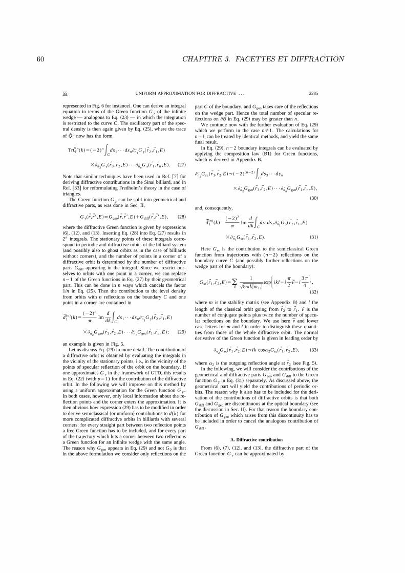
60 CHAPITRE 3. FACETTES ET DIFFRACTION
represented in Fig. 6 for instance!. One can derive an integralequation in terms of the Green function Gg of the infinitewedge — analogous to Eq. ~23! — in which the integrationis restricted to the curve C . The oscillatory part of the spec-tral density is then again given by Eq. ~25!, where the traceof Qn now has the form
TrQn~k !5~22 !nECds1•••dsn]nW 1Gg~rW2 ,rW1 ,E !
3]nW 2Gg~rW3 ,rW2 ,E !•••]nW nGg~rW1 ,rWn ,E !. ~27!
Note that similar techniques have been used in Ref. @7# forderiving diffractive contributions in the Sinai billiard, and inRef. @33# for reformulating Fredholm’s theory in the case oftriangles.
The Green function Gg can be split into geometrical anddiffractive parts, as was done in Sec. II,
Gg~rW ,rW8,E !5Ggeo~rW ,rW8,E !1Gdiff~rW ,rW8,E !, ~28!
where the diffractive Green function is given by expressions~6!, ~12!, and ~13!. Inserting Eq. ~28! into Eq. ~27! results in2n integrals. The stationary points of these integrals corre-spond to periodic and diffractive orbits of the billiard system~and possibly also to ghost orbits as in the case of billiardswithout corners!, and the number of points in a corner of adiffractive orbit is determined by the number of diffractiveparts Gdiff appearing in the integral. Since we restrict our-selves to orbits with one point in a corner, we can replacen21 of the Green functions in Eq. ~27! by their geometricalpart. This can be done in n ways which cancels the factor1/n in Eq. ~25!. Then the contribution to the level densityfrom orbits with n reflections on the boundary C and onepoint in a corner are contained in
d1~n !~k !5
~22 !n
pIm
d
dkECds1•••dsn]nW 1Gg~rW2 ,rW1 ,E !
3]nW 2Ggeo~rW3 ,rW2 ,E !•••]nW nGgeo~rW1 ,rWn ,E !; ~29!
an example is given in Fig. 5.Let us discuss Eq. ~29! in more detail. The contribution of
a diffractive orbit is obtained by evaluating the integrals inthe vicinity of the stationary points, i.e., in the vicinity of thepoints of specular reflection of the orbit on the boundary. Ifone approximates Gg in the framework of GTD, this resultsin Eq. ~22! ~with p51) for the contribution of the diffractiveorbit. In the following we will improve on this method byusing a uniform approximation for the Green function Gg .In both cases, however, only local information about the re-flection points and the corner enters the approximation. It isthen obvious how expression ~29! has to be modified in orderto derive semiclassical ~or uniform! contributions to d(k) formore complicated diffractive orbits in billiards with severalcorners: for every straight part between two reflection pointsa free Green function has to be included, and for every partof the trajectory which hits a corner between two reflectionsa Green function for an infinite wedge with the same angle.The reason why Ggeo appears in Eq. ~29! and not G0 is thatin the above formulation we consider only reflections on the
part C of the boundary, and Ggeo takes care of the reflectionson the wedge part. Hence the total number of specular re-flections on ]B in Eq. ~29! may be greater than n .
We continue now with the further evaluation of Eq. ~29!which we perform in the case nÞ1. The calculations forn51 can be treated by identical methods, and yield the samefinal result.
In Eq. ~29!, n22 boundary integrals can be evaluated byapplying the composition law ~B1! for Green functions,which is derived in Appendix B:
]nW 2Gsc~rW1,rW2,E !'~22 !~n22 !ECds3•••dsn
3]nW 2Ggeo~rW3,rW2 ,E !•••]nW nGgeo~rW1,rWn,E !,
~30!
and, consequently,
d1~n !~k !5
~22 !2
pIm
d
dkECds1ds2]nW 1Gg~rW2 ,rW1 ,E !
3]nW 2Gsc~rW1 ,rW2 ,E !. ~31!
Here Gsc is the contribution to the semiclassical Greenfunction from trajectories with (n22) reflections on theboundary curve C ~and possibly further reflections on thewedge part of the boundary!:
Gsc~rW1 ,rW2 ,E !5(j
1
A8pkum12uexpH ikl2i
p
2n2i
3p
4 J ,~32!
where m is the stability matrix ~see Appendix B! and l thelength of the classical orbit going from rW2 to rW1. n is thenumber of conjugate points plus twice the number of specu-lar reflections on the boundary. We use here n and lowercase letters for m and l in order to distinguish these quanti-ties from those of the whole diffractive orbit. The normalderivative of the Green function is given in leading order by
]nW 2Gsc~rW1 ,rW2 ,E !'ik cosa2Gsc~rW1 ,rW2 ,E !, ~33!
where a2 is the outgoing reflection angle at rW2 ~see Fig. 5!.In the following, we will consider the contributions of the
geometrical and diffractive parts Ggeo and Gdiff to the Greenfunction Gg in Eq. ~31! separately. As discussed above, thegeometrical part will yield the contributions of periodic or-bits. The reason why it also has to be included for the deri-vation of the contributions of diffractive orbits is that bothGdiff and Ggeo are discontinuous at the optical boundary ~seethe discussion in Sec. II!. For that reason the boundary con-tribution of Ggeo which arises from this discontinuity has tobe included in order to cancel the analogous contribution ofGdiff .
A. Diffractive contribution
From ~6!, ~7!, ~12!, and ~13!, the diffractive part of theGreen function Gg can be approximated by
55 2285UNIFORM APPROXIMATION FOR DIFFRACTIVE . . .
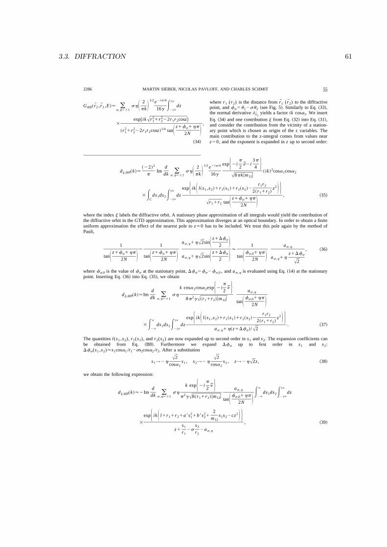
3.3. DIFFRACTION 61
Gdiff~rW2 ,rW1 ,E !' (s ,h561
shS 2
pk D1/2 e2ip/4
16gE
2i`
i`
dz
3
exp$ikAr121r2
222r1r2cosz%
~r121r2
222r1r2cosz !
1/4 tanS z1fs1hp
2N D ,~34!
where r1 (r2) is the distance from rW1 (rW2) to the diffractivepoint, and fs5u12su2 ~see Fig. 5!. Similarly to Eq. ~33!,the normal derivative ]nW 1 yields a factor ik cosa1. We insert
Eq. ~34! and one contribution j from Eq. ~32! into Eq. ~31!,and consider the contribution from the vicinity of a station-ary point which is chosen as origin of the s variables. Themain contribution to the z-integral comes from values nearz50, and the exponent is expanded in z up to second order:
dj ,diff~k !'~22 !2
pIm
d
dk (s ,h561
shS 2
pk D1/2 e2ip/4
16g
expH 2ip
2n2i
3p
4 JA8pkum12u
~ ik !2cosa1cosa2
3ECds1ds2E
2i`
i`
dz
expH ikS l~s1 ,s2!1r1~s1!1r2~s2!2
r1r22~r11r2!
z2D JAr11r2 tanS z1fs1hp
2N D , ~35!
where the index j labels the diffractive orbit. A stationary phase approximation of all integrals would yield the contribution ofthe diffractive orbit in the GTD approximation. This approximation diverges at an optical boundary. In order to obtain a finiteuniform approximation the effect of the nearest pole to z50 has to be included. We treat this pole again by the method ofPauli,
1
tanS z1fs1hp
2N D5
1
tanS z1fs1hp
2N Das ,h1hA2sinS z1Dfs
2 Das ,h1hA2sinS z1Dfs
2 D '1
tanS fs ,01hp
2N Das ,h
as ,h1hz1Dfs
A2
, ~36!
where fs ,0 is the value of fs at the stationary point, Dfs5fs2fs ,0 , and as ,h is evaluated using Eq. ~14! at the stationarypoint. Inserting Eq. ~36! into Eq. ~35!, we obtain
dj ,diff~k !'Imd
dk (s ,h561
sh
k cosa1cosa2expH 2ip
2n J
8p2gA~r11r2!um12u
as ,h
tanS fs ,01hp
2N D
3E2`
`
ds1ds2E2i`
i`
dz
expH ikS l~s1 ,s2!1r1~s1!1r2~s2!2
r1r22~r11r2!
z2D Jas ,h1h~z1Dfs!/A2
. ~37!
The quantities l(s1 ,s2), r1(s1), and r2(s2) are now expanded up to second order in s1 and s2. The expansion coefficients canbe obtained from Eq. ~B8!. Furthermore we expand Dfs up to first order in s1 and s2:Dfs(s1 ,s2)'s1cosa1 /r12ss2cosa2 /r2. After a substitution
s1→2hA2
cosa1s1 , s2→2h
A2
cosa2s2 , z→2hA2z , ~38!
we obtain the following expression:
dj ,diff~k !'2Imd
dk (s ,h561
sh
k expH 2ip
2n J
p2gA8~r11r2!um12u
as ,h
tanS fs ,01hp
2N D E2`
`
ds1ds2E2i`
i`
dz
3
expH ikS l1r11r21a8s121b8s2
21
2
m12s1s22cz2D J
z1s1r1
2ss2r2
2as ,h
, ~39!
2286 55MARTIN SIEBER, NICOLAS PAVLOFF, AND CHARLES SCHMIT
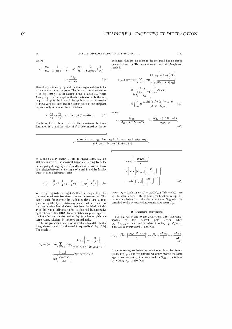
62 CHAPITRE 3. FACETTES ET DIFFRACTION
where
a85
m11
m122
2
R1cosa11
1
r1, b85
m22
m122
2
R2cosa21
1
r2,
c5
r1r2r11r2
. ~40!
Here the quantities r1, r2, and l without argument denote thevalues at the stationary point. The derivative with respect tok in Eq. ~39! yields in leading order a factor iL , whereL5r11r21l is the length of the diffractive orbit. In the nextstep we simplify the integrals by applying a transformationof the s variables such that the denominator of the integranddepends only on one of the s variables:
s5s1r1
2ss2r2, s85dr2s11~12sd !r1s2 . ~41!
The form of s8 is chosen such that the Jacobian of the trans-formation is 1, and the value of d is determined by the re-
quirement that the exponent in the integrand has no mixedquadratic term s8s . The evaluations are done with Maple andresult in
dj ,diff~k !'2Re (s ,h561
sh
kL expH ikL2ip
2n J
p2gA8~r11r2!um12u
3
as ,h
tanS fs ,01hp
2N D E2`
`
ds ds8
3E2i`
i`
dzexp$ik~as21bs822cz2!%
z1s2as ,h, ~42!
where
a5
M 12c
M 122c~ TrM2s2 !, b5
M 122c~ TrM2s2 !
m12r1r2c,
~43!
d5
c~sr1R1cosa1m1122sr1m121sR1cosa1m121r2R1cosa1!
r2R1cosa1@M 122c~ TrM2s2 !#,
M is the stability matrix of the diffractive orbit, i.e., thestability matrix of the classical trajectory starting from thecorner going through rW2 and rW1 and back to the corner. Thereis a relation between n , the signs of a and b and the Maslovindex n of the diffractive orbit
expH 2ip
2n1i
p
4sa1i
p
4sbJ 5i expH 2i
p
2nJ , ~44!
where sa5 sgn(a), sb5 sgn(b). Hence n is equal to n plusthe number of negative signs of a and b ~modulo 4!. Thiscan be seen, for example, by evaluating the s1 and s2 inte-grals in Eq. ~39! by the stationary phase method. Then fromthe composition law of Green functions the Maslov indexn of the whole diffractive orbit is obtained by successiveapplications of Eq. ~B12!. Since a stationary phase approxi-mation after the transformation, Eq. ~41! has to yield thesame result, relation ~44! follows immediately.
The integral over s8 can now be evaluated, and the doubleintegral over s and z is calculated in Appendix C @Eq. ~C9!#.The result is
dj ,diff~k !'2Re (s ,h561
shts
L expH ikL2ip
2n J
gA8~r11r2!um12b~a2c !u
3
uas ,hu
tanS fs ,01hp
2N D eip~11sa1sb1ts!/4
3expH 2
ikacas ,h2
a2c J3F erfcH uaas ,huS k
i~a2c !D 1/2J
2 erfcH uas ,huS kac
i~a2c !D 1/2J G , ~45!
where ts5 sgn(ac/(a2c))5 sgn(M 12 /( TrM2s2)). Aswill be seen in Sec. III B, the first error function in Eq. ~45!is the contribution from the discontinuity of Gdiff which iscanceled by the corresponding contribution from Ggeo .
B. Geometrical contribution
For a given s and h the geometrical orbit that corre-sponds to the nearest pole arises whenfs22ns ,hg52hp , and it exists if h(2ns ,hg2fs),p .This can be reexpressed in the form
as ,h5A2cosS fs ,022ns ,hg
2 D.2A2sinhDfs
2'2
hDfs
A2.
~46!
In the following we derive the contribution from the discon-tinuity of Ggeo . For that purpose we apply exactly the sameapproximations to Ggeo that were used for Gdiff . This is doneby writing Ggeo in the form
55 2287UNIFORM APPROXIMATION FOR DIFFRACTIVE . . .

3.3. DIFFRACTION 63
Ggeo~rW2 ,rW1 ,E !
'2 (s ,h561
sQ~A !S 2
pk D1/2e ip/4
4
3
exp$ikAr121r2
222r1r2cos~fs22ns ,hg !%
~r121r2
222r1r2cos~fs22ns ,hg !!1/4
52 (s ,h561
sQ~A !S 2
pk D1/2e2ip/4
16g
3 R dzexp$ikAr1
21r2
222r1r2cosz%
~r121r2
222r1r2cosz !
1/4 tanS z1fs1hp
2N D ,~47!
where A5as ,h1A2sin(hDfs /2). The integration contour ofthe z integral encircles the nearest pole to z50 counterclock-wise. Expression ~47! differs from Eq. ~34! only by a factor(2h), the Q function and the integration contour. We repeatnow all the steps from Eqs. ~35!–~42!. The only difference isa multiplicative factor (2h) which results from the substi-tution z→2hA2z ~it did not appear previously because ofthe different integration contour!. We arrive at an expressioncorresponding to Eq. ~42!,
2Re (s ,h561
sh
kL expH ikL2ip
2n J
p2gA8~r11r2!um12u
as ,h
tanS fs ,01hp
2N D3E
2`
`
ds ds8 R dz Q~as ,h2s !
3
exp$ik~as21bs822cz2!%
z1s2as ,h. ~48!
The triple integral is denoted by I . The integrals over s8 andz can now be evaluated and result in
I52piS pi
kb D1/2
E2`
as ,hds exp$ikas22ikc~s2as ,h!2%
52piS pi
kb D1/2
E2`
0
ds expH ik~a2c !S s1 aas ,h
a2c D 2
2ikacas ,h
2
a2c J . ~49!
We are interested only in the boundary contribution of thegeometrical part. Expression ~48! in general also containscontributions from periodic orbits. This is the case if theintegration range in Eq. ~49! contains a stationary point, i.e.,if aas ,h /(a2c) is positive. Then the stationary point contri-bution has to be subtracted which corresponds to a subtrac-tion of the integral from 2` to ` . For the boundary weobtain contribution
I852 sgn~as ,h!ts 2piS pi
kb D1/2
E0
`
ds
3expH ik~a2c !S s1U aas ,h
a2cU D 22i
kacas ,h2
a2c J52 sgn~as ,h!ts
p2
k
1
Aub~a2c !ue i~p/4!~11sa1sb1ts!
3expH 2ikacas ,h
2
a2c J erfcH uaas ,huS k
i~a2c !D 1/2J ,
~50!
where ts5 sgn„ac/(a2c)…, as before. Substituting I8 forthe triple integral in Eq. ~48! yields
dj ,geo~k !'Re (s ,h561
shts
L expH ikL2ip
2n J
gA8~r11r2!um12b~a2c !u
3
uas ,hu
tanS fs ,01hp
2N D ei~p/4!~11sa1sb1ts!
3expH 2
ikacas ,h2
a2c J3erfcH uaas ,huS k
i~a2c !D 1/2J . ~51!
Comparison with Eq. ~45! shows that this contribution ex-actly cancels the first error function in Eq. ~45!.
C. Joint contribution
We now can write down the final formula of this section.By using the definitions of a , b , and c the sum of Eqs. ~45!and ~51! can be written in the form
dj~k !'2Re (s ,h561
hts
L
p
expH ikL2ip
2msJ
Au TrM2s2u
3
uas ,hu
2NA2tanS fs1hp
2N D3expH 2
ikas ,h2 M 12
TrM2s2 J3erfcH uas ,huS kM 12
i~ TrM2s2 !D 1/2J , ~52!
where we dropped the second index of fs ,0 for simplicity ofnotation. Furthermore, ms5n1(12s)1ks , ts5122ks ,and ks is defined as
2288 55MARTIN SIEBER, NICOLAS PAVLOFF, AND CHARLES SCHMIT

64 CHAPITRE 3. FACETTES ET DIFFRACTION
ks5H 0 ifM 12
TrM2s2.0
1 ifM 12
TrM2s2,0.
~53!
We recall that M in Eqs. ~52! and ~53! is the stabilitymatrix ~at unit energy! of the classical trajectory starting andending at the corner point. n is the number of conjugatepoints of this trajectory, plus two times the number of specu-lar reflections. The definition of ms in terms of n and ks issimilar to the definition of the Maslov index of a periodicorbit in terms of that of the Green function @35#. The sdependence is due to the fact that positive s values are as-sociated with geometrical orbits that are reflected an evennumber of times near the corner, as an optical boundary isapproached, and negative s values with orbits with an oddnumber of bounces. This is explained in more detail in Ap-pendix D. In the limiting case that the diffractive orbit be-comes a periodic orbit, its contribution comes only from oneof the values of s ~the other cancels!, and its stability matrixis M or 2M , depending on whether the number of bouncesof the orbit in the corner is even or odd ~cf. the discussion inSec. IV B!. Thus ms is identical to the Maslov index of theperiodic orbit in these limiting cases.
In terms of the Fresnel integral K formula ~52! can writ-ten in a slightly shorter form,
dj~k !'2Re (s ,h561
hts
L
p
expH ikL2ip
2msJ
Au TrM2s2u
3
uas ,hu
NA2tanS fs1hp
2N D KF uas ,huiksS kuM 12u
u TrM2s2u D1/2G .~54!
Equation ~54! is the main result of this paper. It providesa uniform approximation for the contribution of an isolateddiffractive orbit with a single corner point to the trace for-mula. For completeness we recall several definitions:fs5u12su2, where u1 and u2 are the incoming and out-going angles at the diffractive point ~measured from thesame edge, with u1 and u2P@0,g#) and as ,h is defined by
as ,h5A2cosS fs
22ns ,hg D
with ns ,h5 nintFfs1hp
2g GPZ. ~55!
Note finally that the modified Fresnel function of imaginaryargument ~encountered when ks51) can be computed nu-merically from Eq. ~A3!.
IV. DISCUSSION OF THE RESULT
In this section we discuss properties and the range of va-lidity of formula ~54!. As mentioned above, the derivationhas been done for a specific case ~a wedge connected to a
smooth boundary!, but it is more generally valid because itrelies only on local properties of the system near the consid-ered diffractive orbit ~as usual in semiclassical approxima-tions!. Hence it applies to billiards of any shape, providedthe singularity of the boundary corresponds locally to theintersection of two straight lines. However, the present ap-proach has to be refined if applied to curved edges; we dis-cuss this point in Appendix D. We also remind the readerthat formula ~54! is only valid for single diffraction. Thesame formalism can in principle also be applied to diffractiveorbits with more than one diffractive point; however, theformulas become increasingly more complex. For example,in the case of double diffraction, one has already 16 insteadof four terms, and they also involve double Fresnel integralsas can be inferred from the treatment of diffraction at twowedges in @21#. The formulas can only be simplified if thediffraction in some of the corners can be treated in the GTDapproximation.
Note also, that the factor u TrM22su21/2 in Eq. ~54! di-verges for a parabolic diffractive orbit ~i.e., whenTrM562), and the present approach cannot be used in thiscase. This is very similar to divergences in Gutzwiller’s traceformula due to nonisolated orbits. For diffractive orbits,TrM562 can have several causes; for example, the diffrac-tive orbits can appear in families as is the case in a circularsector, or bifurcations of diffractive orbits can occur, or thediffractive orbit can become a part of a family of periodicorbits when the optical boundary is approached. The lattercase can occur, for example, in triangular billiards. In thiscase it is, however, often possible to treat the divergent part~one of the s values! in the GTD approximation if the dif-fractive orbit is well separated from the torus of periodicorbits, and apply the uniform approximation only to the non-divergent part, as will be demonstrated in a numerical ex-ample in Sec. V.
A. GTD limit
After these basic remarks we now study three simple lim-its of Eq. ~54!. The first one is the geometrical theory ofdiffraction which is valid sufficiently far away from the op-tical boundary. In this limit the argument of the K function islarge, and the function can be replaced by its leadingasymptotic term in Eq. ~A4!. This immediately yields
dj~k !'L
p
D~u1 ,u2!
A8pkuM 12ucos~kL2np/223p/4!, ~56!
which agrees with the general formula ~22! in the case of onediffractive point. Analogous formulas have been derived andtested in @4,6,8#. They have the advantage of allowing one totreat general diffractive problems ~other than wedge diffrac-tion!, and can easily be generalized to multiple diffraction@see Eq. ~22!#. However, they diverge on the optical bound-ary and ~as shown in the examples Secs. V A and V B be-low! they are unable to describe the limit that a diffractiveorbit is close to become a real trajectory.
B. Limit g5p/p
Let us now study the limit that the diffraction angle ggoes to p/p (pPN*). For these values of g there is no
55 2289UNIFORM APPROXIMATION FOR DIFFRACTIVE . . .

3.3. DIFFRACTION 65
diffraction, since the corner can be treated by the method ofimages. As a consequence, the contributions of most diffrac-tive orbits disappear, but there are also diffractive orbitswhich are replaced by periodic orbits which contribute to thelevel density according to the Gutzwiller trace formula. Theircontribution can be obtained from the diffractive contribu-tion ~54! in the limit g→p/p . The situation is actuallyslightly more complicated, since the diffractive contributionof these orbits for angles g5p/p1e is discontinuous ate50 ~it changes sign!. The reason for this is that periodicorbits split from the diffractive orbit as e goes through zero~for example, as the billiard is deformed!, which can be con-sidered as a kind of bifurcation. As a consequence both dif-fractive and periodic orbit contributions are discontinuous ate50, but their sum remains continuous. In order to discussthis in more detail we have to consider the cases of odd andeven p separately.
~i! Case g5(p/2p)1e . In the limit e50 the contribu-tions from the two h values cancel for s521. The sameoccurs for s511, except if u25u1. If this condition is ful-filled, one obtains
dj~k !→ sgn~e !t ~1 !dpo~k !, ~57!
where
dpo~k !5
L
p
cos~kL2m ~1 !p/2!
u TrM22u1/2when g5
p
2p. ~58!
The discontinuity in Eq. ~57! at e50 is directly related tothe appearance of periodic orbits. This can be seen from thediscussion in Sec. III B: in Eq. ~49! one has contributions ofperiodic orbits in the vicinity of the diffractive orbit ifas ,hts.0, and the periodic orbits coincide with the diffrac-tive orbit when as ,h50. For the considered case the aboveinequality is equivalent to 2 sgn(e)t (1).0. Hence when egoes through zero, two periodic orbits appear ~or disappear!,one for each value of h , assuring the continuity of the sum ofcontributions at e50.
~ii! Case g5p/(2p11)1e . Now the two contributionsto s511 cancel as e→0, and for s521 there is only acontribution if u25g2u1. This contribution is of the form
dj~k !→ sgn~e !t ~2 !dpo~k !, ~59!
and the periodic orbit contribution now is given by
dpo~k !5
L
p
cos~kL2m ~2 !p/2!
u TrM12u1/2when g5
p
2p11.
~60!
Comparing with Eq. ~58!, the reason for the change ofsign of M is the odd number of classical reflections on thevertex in the case g5p/(2p11). Generally, the stabilitymatrix M of the closed trajectory in Eq. ~54! becomes equalto plus @minus# the monodromy matrix of the periodic orbitwhen g is p/(2p) @p/(2p11)#. The explanation of the dis-continuity of Eq. ~59! is the same as above, with the onlydifference that the condition for the existence of neighboringperiodic orbits can now be expressed by 2 sgn(e)t (2).0.
In billiards with corners one has therefore a new kind ofbifurcation: the continuity of wave mechanics ~in the semi-
classical approximation! is not enforced by complex trajec-tories but by diffractive orbits. This effect will be demon-strated in the examples below.
C. In the vicinity of an optical boundary
The case that a diffractive orbit lies on an optical bound-ary, or crosses an optical boundary when the billiard is de-formed, is very similar to the case g→p/p . Again the dif-fractive orbit contributes on the optical boundary at the sameorder of k as a periodic orbit, but now only with half theamplitude of a periodic orbit. The diffractive contribution isagain discontinuous since it changes sign as an opticalboundary is crossed, and the reason for this is that a periodicorbit arises which bifurcates from the diffractive orbit. Morespecifically, let us consider the case that for a given value ofs and h one has fs22ns ,hg1hp5e , where e is small. Inthe limit e→0 the contribution from these values of s andh to the spectral density is given by
212 hts sgn~e !dpo~k !
where dpo~k !5
L
p
cos~kL2msp/2!
Au TrM22su, ~61!
and one can verify that the discontinuity of Eq. ~61! is due toa neighboring periodic orbit which coincides with the dif-fractive orbit at e50. As above, the condition for the exist-ence of the periodic orbit is as ,hts.0 which now is equiva-lent to hets.0.
V. SOME EXAMPLES
In this section we illustrate the results of the last sectionswith several examples. We study mainly a billiard consistingof a wedge of opening angle g whose two edges are con-nected by an arc of constant radius of curvature R . Theangles between arc and wedge are chosen to be p/3 on bothsides. If h denotes the ‘‘height’’ of this billiard ~see Fig. 6!then R5hsin(g/2)„sin(g/2)2 1
2…21. This billiard has only one
diffractive corner ~at point S of Fig. 6! and the curvatureensures that the shortest diffractive and periodic orbits haveTrMÞ62 ~they are displayed in Fig. 6!. In the followingwe call this billiard a ‘‘rounded triangle (p/3,p/3,g).’’
For numerical convenience we restrict ourselves to anglesof the form g5pp/q with (p ,q)PN
2. The quantum energiesare determined by expanding the wave functions aroundpoint S in ‘‘partial waves’’ which are Bessel functions timesa sinusoidal function of the angle:
c~r ,u !5 (n51
nmax
Jnq/p~kr !sinS nqp u D . ~62!
Equation ~62! automatically fulfills the Dirichlet conditionon the straight faces of the billiard. The boundary conditionon the arc opposite to S is enforced in a manner identical tothe improved point matching method presented in @34#. Thisresults in a secular equation whose solutions are the eigen-levels of the system. We have tested the numerical stabilityof our procedure by varying the number nmax of partialwaves included in the expansion ~typically nmax
2290 55MARTIN SIEBER, NICOLAS PAVLOFF, AND CHARLES SCHMIT

66 CHAPITRE 3. FACETTES ET DIFFRACTION
' nint@pkh/q#). For each of the values of g studied belowwe have computed the first 2000 eigenlevels, and wechecked that they were determined with an accuracy of theorder of 1/1000 of the mean level spacing.
In order to visualize the importance of periodic and dif-fractive orbits we study in the following the regularized Fou-rier transform of the level density,
F~x !5E0
kmaxAk e ikx2ak2d~k !dk . ~63!
kmax is the last eigenvalue computed numerically and we takehere a510/kmax
2 The multiplicative factor Ak in Eq. ~63! isincluded in order to cancel the singularity at k50 of a con-tribution of type ~56!. F(x) is denoted FQM(x) if we use inEq. ~63! the exact quantum spectrum. It is denoted FUA(x)@FGTD(x)#, when Eq. ~54! @Eq. ~56!# is used together withthe periodic orbit contributions ~B21!.
A. g near p/2
This case is relevant to Sec. IV B above. For g,p/2 theshortest orbit is a periodic one and has length L152h sing.It disappears as soon as g.p/2. For gÞp/2, one also has adiffractive orbit of length L252h ~see Fig. 6!. Wheng5p/2 these orbits coalesce, and give a single periodic orbitof length 2h . Their contribution to the level density is con-tinuous at g5p/2 as explained above: the contribution of
L2 is discontinuous @cf. Eq. ~57!#, and this exactly cancelsthe discontinuity due to the disappearance of the orbit L1 andits time reverse.
We determined the spectrum numerically for g57p/15and 8p/15. The corresponding moduli of the Fourier trans-form uF(x)u are plotted in Figs. 7 and 8. In these figures thesolid lines correspond to uFQM(x)u, the long dashed lines touFUA(x)u, and the short dashed line to uFGTD(x)u. Thelengths of the included orbits are marked with back arrows.One notices the failure of GTD and the excellent agreementof approximation ~54! with the exact result @the agreementremains equally good when plotting the real and imaginarypart of F(x)#. As stated above, it can be seen that in thevicinity of an optical boundary diffractive and periodic orbitscontribute in the same order to the level density.
B. g near p
This case also pertains to the discussion of Sec. IV B, butnow in the vicinity of g5p/(2p11). Again the diffractiveorbit ensures continuity of semiclassical mechanics wheng5p: the two periodic orbits L4 and L48 of Fig. 6 disappearas soon as g,p , and the contribution of L2 is discontinuousat g5p , but the joint contribution is continuous. Here wecomputed numerically the levels for g519p/20 and presentthe results for uF(x)u and Re$F(x)% in Fig. 9. Again one canverify the failure of the geometrical theory of diffraction andthe excellent agreement between Eq. ~54! and the quantumresult.
C. Triangle „p/4,p/6,7p/12…
In this subsection we depart from the previous examplesand study the spectrum of a straight triangular billiard withangles (p/4,p/6,7p/12), which has one diffractive wedge
FIG. 6. Shortest periodic and diffractive orbits in the ‘‘roundedtriangular billiard’’ studied in Sec. V. For the diffractive orbit, thediffractive point is marked with a black point. The upper plot de-fines the geometry and the notations.
FIG. 7. Modulus uF(x)u of the Fourier transform of the leveldensity — see Eq. ~63! — for the rounded triangle(p/3,p/3,g57p/15). The solid line corresponds to FQM(x), thelong dashed line to FUA(x), and the short dashed line to FGTD(x)~see the text!. The arrows mark the lengths of the diffractive andperiodic orbits. The scale of lengths and wave vectors is fixed bytaking h51.
55 2291UNIFORM APPROXIMATION FOR DIFFRACTIVE . . .
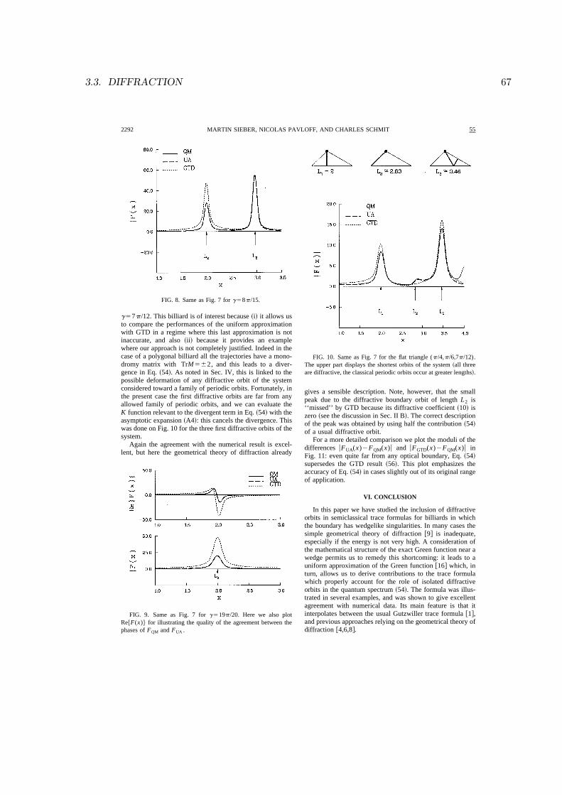
3.3. DIFFRACTION 67
g57p/12. This billiard is of interest because ~i! it allows usto compare the performances of the uniform approximationwith GTD in a regime where this last approximation is notinaccurate, and also ~ii! because it provides an examplewhere our approach is not completely justified. Indeed in thecase of a polygonal billiard all the trajectories have a mono-dromy matrix with TrM562, and this leads to a diver-gence in Eq. ~54!. As noted in Sec. IV, this is linked to thepossible deformation of any diffractive orbit of the systemconsidered toward a family of periodic orbits. Fortunately, inthe present case the first diffractive orbits are far from anyallowed family of periodic orbits, and we can evaluate theK function relevant to the divergent term in Eq. ~54! with theasymptotic expansion ~A4!: this cancels the divergence. Thiswas done on Fig. 10 for the three first diffractive orbits of thesystem.
Again the agreement with the numerical result is excel-lent, but here the geometrical theory of diffraction already
gives a sensible description. Note, however, that the smallpeak due to the diffractive boundary orbit of length L2 is‘‘missed’’ by GTD because its diffractive coefficient ~10! iszero ~see the discussion in Sec. II B!. The correct descriptionof the peak was obtained by using half the contribution ~54!of a usual diffractive orbit.
For a more detailed comparison we plot the moduli of thedifferences uFUA(x)2FQM(x)u and uFGTD(x)2FQM(x)u inFig. 11: even quite far from any optical boundary, Eq. ~54!supersedes the GTD result ~56!. This plot emphasizes theaccuracy of Eq. ~54! in cases slightly out of its original rangeof application.
VI. CONCLUSION
In this paper we have studied the inclusion of diffractiveorbits in semiclassical trace formulas for billiards in whichthe boundary has wedgelike singularities. In many cases thesimple geometrical theory of diffraction @9# is inadequate,especially if the energy is not very high. A consideration ofthe mathematical structure of the exact Green function near awedge permits us to remedy this shortcoming: it leads to auniform approximation of the Green function @16# which, inturn, allows us to derive contributions to the trace formulawhich properly account for the role of isolated diffractiveorbits in the quantum spectrum ~54!. The formula was illus-trated in several examples, and was shown to give excellentagreement with numerical data. Its main feature is that itinterpolates between the usual Gutzwiller trace formula @1#,and previous approaches relying on the geometrical theory ofdiffraction @4,6,8#.
FIG. 8. Same as Fig. 7 for g58p/15.
FIG. 9. Same as Fig. 7 for g519p/20. Here we also plotRe$F(x)% for illustrating the quality of the agreement between thephases of FQM and FUA .
FIG. 10. Same as Fig. 7 for the flat triangle (p/4,p/6,7p/12).The upper part displays the shortest orbits of the system ~all threeare diffractive, the classical periodic orbits occur at greater lengths!.
2292 55MARTIN SIEBER, NICOLAS PAVLOFF, AND CHARLES SCHMIT
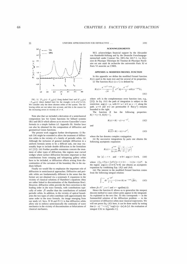
68 CHAPITRE 3. FACETTES ET DIFFRACTION
Note also that we included a derivation of a semiclassicalcomposition law for Green functions for billiard systems~B1! and ~B13! which allows us to recover Gutzwiller’s traceformula in a simple fashion ~cf. Appendix B!. Similar lawscan also be obtained for the composition of diffractive andgeometrical Green functions.
The present work suggests further developments: ~i! Re-sult ~54! might be extended to allow the treatment of diffrac-tive orbits in the vicinity of a family of periodic orbits. ~ii!Although the inclusion of general multiple diffraction in auniform formula seems to be a difficult task, one may rea-sonably hope to include double diffraction in the formalism~cf. @21#!. ~iii! Further possible extensions concern the treat-ment of other types of diffraction, like regions near curvedwedges where surface diffraction becomes important so thatcontributions from creeping and whispering gallery orbitshave to be included, or diffraction effects arising from dis-continuities of the curvature of the boundary like in the sta-dium billiard.
Finally we would like to emphasize the important role ofdiffraction in semiclassical approaches. Diffractive and peri-odic orbits are fundamentally different in the sense that theformer are not obtained via a systematic \ expansion in thevicinity of classical solutions of Hamilton’s equations ~theyare rather linked to discontinuities of the Hamiltonian flow!.However, diffractive orbits provide the first correction to theleading order in the trace formula, with contributions typi-cally of order A\ smaller than the contributions of isolatedperiodic orbits. In addition, in the vicinity of optical bound-aries the two types of orbit contribute with approximately thesame order to the trace formula. An image emerging fromour study ~cf. Secs. IV B and IV C! is that diffractive orbitsallow one to enforce semiclassically the continuity of wavemechanics in the vicinity of discontinuities or bifurcations ofclassical mechanics.
ACKNOWLEDGMENTS
M.S. acknowledges financial support by the Alexandervon Humboldt-Stiftung and by the Deutsche Forschungsge-meinschaft under Contract No. DFG-Ste 241/7-1. La Divi-sion de Physique Theorique de l’Institut de Physique Nucle-aire est une unite de recherche des universites Paris XI etParis VI associee au CNRS.
APPENDIX A: MODIFIED FRESNEL FUNCTION
In this appendix we define the modified Fresnel functionK(z) used in the main text and list several of its properties.
~i! The function K(z) (zPC) is defined by
K~z !5
e2i~z21p/4!
ApEz
`
e iy2dy5
e2iz2
2erfc~e2ip/4z !,
~A1!
where erfc is the complementary error function ~see, e.g.,@25#!. In Eq. ~A1! the path of integration is subject to therestriction arg(y)→a , with 0,a,p/2 as y→` along thepath. a50 and p/2 are permissible if Re(iy2) remainsbounded to the right.
The function K has the following properties:K(1`)50, K(0)5 1
2,
K~z !1K~2z !5e2iz2, ~A2!
and
K~ z !1K~2iz !5e iz2, ~A3!
where the bar denotes complex conjugation.~ii! By successive integrations by parts one obtains the
following asymptotic expansion:
K~z !5
e ip/4
2zAp(n50
1` S 12 DnS 2i
z2 D n
for uzu→1` and 2p/4, arg~z !,3p/4, ~A4!
where ( 12)n5G(n112)/G(
12)51333•••3(2n21)/2n. In
the region arg(z)P]3p/4,7p/4@ one obtains an asymptoticexpansion by combining Eqs. ~A2! and ~A4!.
~iii! The interest in the modified Fresnel function comesfrom the following integral relation:
E2`
1`
dte2bt2
t2z52 itp K~te2ip/4Abz !, ~A5!
where bPR1, zPC and t5 sgn„Im(z)….
Hence the function K allows us to generalize the steepestdescent method to cases where poles appear in the integrand.As explained in the text ~Sec. II! this corresponds — in theSommerfeld solution of the diffraction problem — to theoccurrence of diffractive orbits near classical trajectories. Wewill not prove Eq. ~A5! here, it can be done easily by notingthat (t2z)21
5it*01`exp@it (z2t)x# dx @cf. the evaluation of
integral ~C6! in Appendix C#.
FIG. 11. uFUA(x)2F QM(x)u ~long dashed line! and uF GTD(x)2FQM(x)u ~short dashed line! for the triangle (p/4,p/6,7p/12).We consider only the three shortest orbits of the system. The fol-lowing orbits are not taken into account, and this is the reason forthe increasing errors in vicinity of x'4.
55 2293UNIFORM APPROXIMATION FOR DIFFRACTIVE . . .

3.3. DIFFRACTION 69
APPENDIX B: COMPOSITION LAW FOR GREENFUNCTIONS
In this appendix we derive a simple semiclassical compo-sition law for Green functions which is expressed by inte-grals over the boundary ]B of the billiard. The formulasestablished below are simple, and are connected to Balianand Bloch’s multiple reflexion expansion @2#. Although theyare clear from a semiclassical interpretation of this expansion~see, e.g., Refs. @3, 27, 28#! we include a derivation for com-pleteness. The composition law can be used in order to sim-plify expressions obtained from the boundary elementmethod @cf. Eq.~31!#. We first prove the semiclassical ver-sion and then give the exact formulation of this law due toBalian and Bloch. We further show that it allows us to deriveGutzwiller’s trace formula in a straightforward manner.
We assume in this appendix that the boundary ]B issmooth everywhere. The semiclassical version of the compo-sition law has the form
~22 !nE]Bds1•••dsnG0~rW1 ,rW8,E !]nW 1G0~rW2 ,rW1 ,E !•••
3]nW nG0~rW ,rWn ,E !'Gsc~n !~rW ,rW8,E !, ~B1!
where rW i5rW(s i). The approximate sign signifies that theevaluation is done by approximating the free Green functionG0 by its leading asymptotic term for large argument, andevaluating the integrals in the stationary phase approxima-tion. The function Gsc
(n)(rW ,rW8,E) on the right-hand side of Eq.~B1! is the part of the semiclassical Green function from alltrajectories with n bounces on the boundary between rW8 andrW ,
Gsc~n !~rW ,rW8,E !5(
jn
1
A8pkuM 12~n !u
3expH ikl ~n !2i
p
2n ~n !
2i3p
4 J . ~B2!
Here l (n) denotes the length of the trajectory, n (n) is thenumber of conjugate points from rW8 to rW plus twice the num-ber of reflections on the boundary, and M (n) is the stabilitymatrix for unit energy. An index jn of the above quantitieshas been omitted in order to simplify the notations.
Equation ~B1! is proven by mathematical induction. Forn50 it is correct since
G0~rW ,rW8,E !'Gsc~0 !~rW ,rW8,E !, ~B3!
and one has to show that
I:5~22 !E]Bds1Gsc
~n !~rW1 ,rW8,E !]nW 1G0~rW ,rW1 ,E !
'Gsc~n11 !~rW ,rW8,E !. ~B4!
We will use the following notation at a point rW i of the bound-ary: primed quantities correspond to the incoming trajectory,and unprimed quantities to the outgoing trajectory. We will
denote the momentum of a classical trajectory by a vectorpW of modulus k , whose direction is the direction of propaga-tion of the classical particle. The momentum of an outgoingtrajectory is pW i , and a i is the angle between the normalvector nW i of the boundary ~which points outside! and 2pW i .The momentum of an incoming trajectory is pW i8, and a i8 is
the angle between nW i and pW i8. For this choice a i8 and a i bothlie in the interval between 2p/2 and p/2. In terms of thelocal coordinate systems of the trajectories with coordinatesparallel and perpendicular to the trajectory, the tangentialand normal vectors of the boundary can be written as
nW i52cosa ieW i1sina ieW'5cosa i8eW i82sina i8eW'8 ,
~B5!
tW i52sina ieW i2cosa ieW'5sina i8eW i81cosa i8eW'8 .
We continue by evaluating the integral in Eq. ~B4! using thestationary phase approximation. The normal derivative of theGreen function is given in leading semiclassical order by
]nW iG0~rW i11 ,rW i ,E !'2inW i•pW iGsc~0 !~rW i11 ,rW i ,E !
5ik cosa iGsc~0 !~rW i11 ,rW i ,E !, ~B6!
and in Eq. ~B4! the stationary points are determined by thecondition
05
d
ds1@ l ~0 !~rW ,rW1!1l ~n !~rW1 ,rW8!#
5 tW•F2
pW 1k
1
pW 18
kG
5sina11sina18 , ~B7!
i.e., by a152a18 , which is the condition for elastic reflec-tion. The sum over all stationary points thus expresses theintegral I by a sum over all trajectories with n11 reflectionson the boundary. In Eq. ~B7! and in the following, the lengthis given two arguments when it is necessary to specify thestarting and end point of the trajectory.
For the determination of the second derivatives of thelengths at a boundary point s i , one has to evaluate the de-rivatives of the angles a i and a i8 which consist of two parts.One is due to the change of the normal vector with s i , andone to the change of the direction of the trajectories:
d2l ~n !~rW i ,rW i21!
ds i2 5cosa i8
da i8
ds i
5cosa i8S 2
1
R i1
cosa i8
k
dp i'
8
dq i'
8D
52
cosa i8
R i1
cos2a i8M 22~n !
M 12~n ! ,
~B8!
2294 55MARTIN SIEBER, NICOLAS PAVLOFF, AND CHARLES SCHMIT
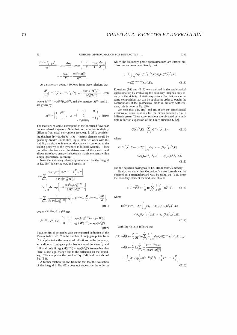
70 CHAPITRE 3. FACETTES ET DIFFRACTION
d2l ~n !~rW i11 ,rW i!
ds i2 5cosa i
da i
ds i5cosa iS 2
1
R i2
cosa i
k
dp i'
dq i'
D52
cosa i
R i1
cos2a iM 11~n !
M 12~n ! .
At a stationary point, it follows from these relations that
d2
ds12 @ l ~0 !~rW ,rW1!1l ~n !~rW1 ,rW8!#52
cos2a1M 12~n11 !
M 12~0 !M 12
~n ! , ~B9!
where M (n11)5M (0)B1M
(n), and the matrices M (0) and B1are given by
M ~0 !5S 1 l ~0 !
0 1 D , B15S 21 0
2
R1cosa121D . ~B10!
The matrices M and B correspond to the linearized flow nearthe considered trajectory. Note that our definition is slightlydifferent from usual conventions ~see, e.g., @1,35#!: consider-ing that here upW u5k , the M 12 (M 21) matrix element would begenerally divided ~multiplied! by k . Here we work with thestability matrix at unit energy: this choice is connected to thescaling property of the dynamics in billiard systems. It doesnot affect the trace and the determinant of the matrix, andallows us to have energy-independent matrix elements with asimple geometrical meaning.
Now the stationary phase approximation for the integralin Eq. ~B4! is carried out, and results in
I' (jn11
cosa1expH ikl ~n11 !2i
p
2n ~n !J
4pAuM 12~0 !M 12
~n !u
3E]Bds1expH 2ik
cos2a1M 12~n11 !
2M 12~0 !M 12
~n ! s12J
' (jn11
1
A8pkuM 12~n11 !u
expH ikl ~n11 !2i
p
2n ~n11 !
2i3p
4 J ,~B11!
where l (n11)5l (0)1l (n) and
n ~n11 !5n ~n !
121H 1 if sgn~M 12~n11 !!5 sgn~M 12
~n !!
0 if sgn~M 12~n11 !!Þ sgn~M 12
~n !!.
~B12!
Equation ~B12! coincides with the expected definition of theMaslov index: n (n11) is the number of conjugate points fromrW8 to rW plus twice the number of reflections on the boundary;an additional conjugate point has occurred between rW1 andrW if and only if sgn(M 12
(n11))5 sgn(M 12(n)) ~remember that
there is one sign change due to the reflection on the bound-ary!. This completes the proof of Eq. ~B4!, and thus also ofEq. ~B1!.
A further relation follows from the fact that the evaluationof the integral in Eq. ~B1! does not depend on the order in
which the stationary phase approximations are carried out.Thus one can conclude directly that
~22 !E]Bds1Gsc
~n !~rW1 ,rW8,E !]nW 1Gsc~m !~rW ,rW1 ,E !
'Gsc~n1m11 !~rW ,rW8,E !. ~B13!
Equations ~B1! and ~B13! were derived in the semiclassicalapproximation by evaluating the boundary integrals only lo-cally in the vicinity of stationary points. For that reason thesame composition law can be applied in order to obtain thecontributions of the geometrical orbits in billiards with cor-ners; this is done in Eq. ~30!.
We note that Eqs. ~B1! and ~B13! are the semiclassicalversions of exact relations for the Green function G of abilliard system. These exact relations are obtained by a mul-tiple reflection expansion of the Green function G @2#,
G~rW ,rW8,E !5 (n50
`
G ~n !~rW ,rW8,E !, ~B14!
where
G ~n !~rW ,rW8,E !5~22 !nE]Bds1•••dsnG0~rW1 ,rW8,E !
3]nW 1G0~rW2 ,rW1 ,E !•••]nW nG0~rW ,rWn ,E !,
~B15!
and the equation analogous to Eq. ~B13! follows directly.Finally, we show that Gutzwiller’s trace formula can be
obtained in a straightforward way by using Eq. ~B1!. Fromthe boundary element method, one obtains
d~k !5 d~k !1
1
pIm(
n51
`1
n
d
dkTrQn~k !, ~B16!
where
TrQn~k !5~22 !nE]Bds1•••dsn]nW 1G0~rW2 ,rW1 ,E !
3]nW 2G0~rW3 ,rW2 ,E !•••]nW nG0~rW1 ,rWn ,E !.
~B17!
With Eq. ~B1!, it follows that
d~k !' d~k !2
2
p
d
dkIm(
n51
`1
nE]Bds]nW 8Gsc
~n21 !~rW ,rW8,E !urW5rW8
' d~k !2
2
pRe(
n52
`1
n
kl ~n21 !cosa
A8pkuM 12~n !u
3E]Bds expH ikl ~n21 !~rW ,rW !2i
p
2n ~n21 !
2ip
4 J .~B18!
55 2295UNIFORM APPROXIMATION FOR DIFFRACTIVE . . .
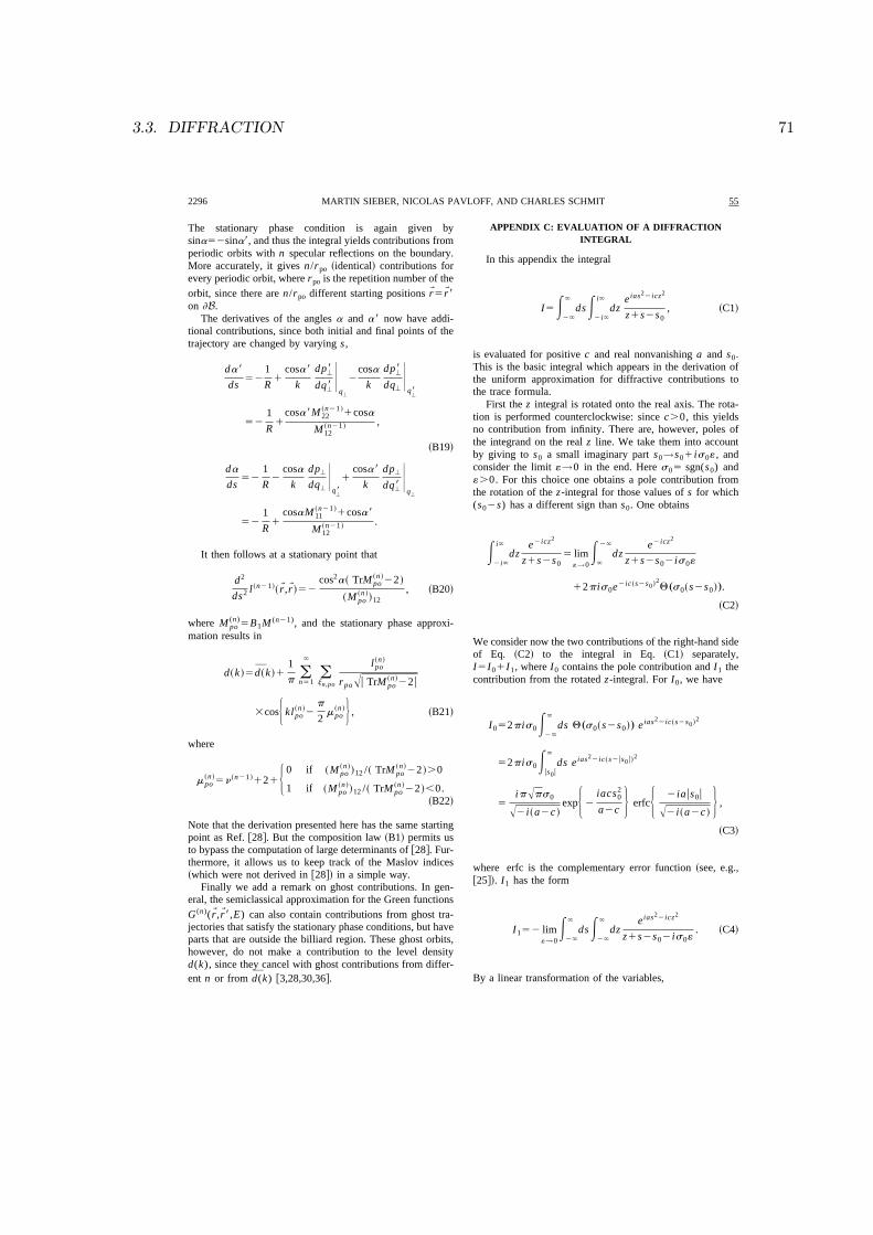
3.3. DIFFRACTION 71
The stationary phase condition is again given bysina52sina8, and thus the integral yields contributions fromperiodic orbits with n specular reflections on the boundary.More accurately, it gives n/rpo ~identical! contributions forevery periodic orbit, where rpo is the repetition number of theorbit, since there are n/rpo different starting positions rW5rW8
on ]B.The derivatives of the angles a and a8 now have addi-
tional contributions, since both initial and final points of thetrajectory are changed by varying s ,
da8
ds52
1
R1
cosa8
k
dp'8
dq'8Uq
'
2
cosa
k
dp'8
dq'
Uq
'8
52
1
R1
cosa8M 22~n21 !
1cosa
M 12~n21 ! ,
~B19!
da
ds52
1
R2
cosa
k
dp'
dq'
Uq
'8
1
cosa8
k
dp'
dq'8Uq
'
52
1
R1
cosaM 11~n21 !
1cosa8
M 12~n21 ! .
It then follows at a stationary point that
d2
ds2l ~n21 !~rW ,rW !52
cos2a~ TrM po~n !
22 !
~M po~n !!12
, ~B20!
where M po(n)
5B1M(n21), and the stationary phase approxi-
mation results in
d~k !5 d~k !1
1
p (n51
`
(jn ,po
lpo~n !
rpoAu TrM po~n !
22u
3cosH klpo~n !2
p
2mpo
~n !J , ~B21!
where
mpo~n !
5n ~n21 !121H 0 if ~M po
~n !!12 /~ TrM po~n !
22 !.0
1 if ~M po~n !!12 /~ TrM po
~n !22 !,0.
~B22!
Note that the derivation presented here has the same startingpoint as Ref. @28#. But the composition law ~B1! permits usto bypass the computation of large determinants of @28#. Fur-thermore, it allows us to keep track of the Maslov indices~which were not derived in @28#! in a simple way.
Finally we add a remark on ghost contributions. In gen-eral, the semiclassical approximation for the Green functionsG (n)(rW ,rW8,E) can also contain contributions from ghost tra-jectories that satisfy the stationary phase conditions, but haveparts that are outside the billiard region. These ghost orbits,however, do not make a contribution to the level densityd(k), since they cancel with ghost contributions from differ-ent n or from d(k) @3,28,30,36#.
APPENDIX C: EVALUATION OF A DIFFRACTIONINTEGRAL
In this appendix the integral
I5E2`
`
dsE2i`
i`
dze ias
22icz2
z1s2s0, ~C1!
is evaluated for positive c and real nonvanishing a and s0.This is the basic integral which appears in the derivation ofthe uniform approximation for diffractive contributions tothe trace formula.
First the z integral is rotated onto the real axis. The rota-tion is performed counterclockwise: since c.0, this yieldsno contribution from infinity. There are, however, poles ofthe integrand on the real z line. We take them into accountby giving to s0 a small imaginary part s0→s01is0« , andconsider the limit «→0 in the end. Here s05 sgn(s0) and«.0. For this choice one obtains a pole contribution fromthe rotation of the z-integral for those values of s for which(s02s) has a different sign than s0. One obtains
E2i`
i`
dze2icz2
z1s2s05 lim
«→0E2`
dze2icz2
z1s2s02is0«
12pis0e2ic~s2s0!2Q„s0~s2s0!….
~C2!
We consider now the two contributions of the right-hand sideof Eq. ~C2! to the integral in Eq. ~C1! separately,I5I01I1, where I0 contains the pole contribution and I1 thecontribution from the rotated z-integral. For I0, we have
I052pis0E2`
`
ds Q„s0~s2s0!… eias22ic~s2s0!2
52pis0Eus0u
`
ds e ias22ic~s2us0u!2
5
ipAps0
A2i~a2c !expH 2
iacs02
a2c J erfcH 2iaus0u
A2i~a2c !J ,
~C3!
where erfc is the complementary error function ~see, e.g.,@25#!. I1 has the form
I152 lim«→0
E2`
`
dsE2`
`
dze ias
22icz2
z1s2s02is0«. ~C4!
By a linear transformation of the variables,
2296 55MARTIN SIEBER, NICOLAS PAVLOFF, AND CHARLES SCHMIT
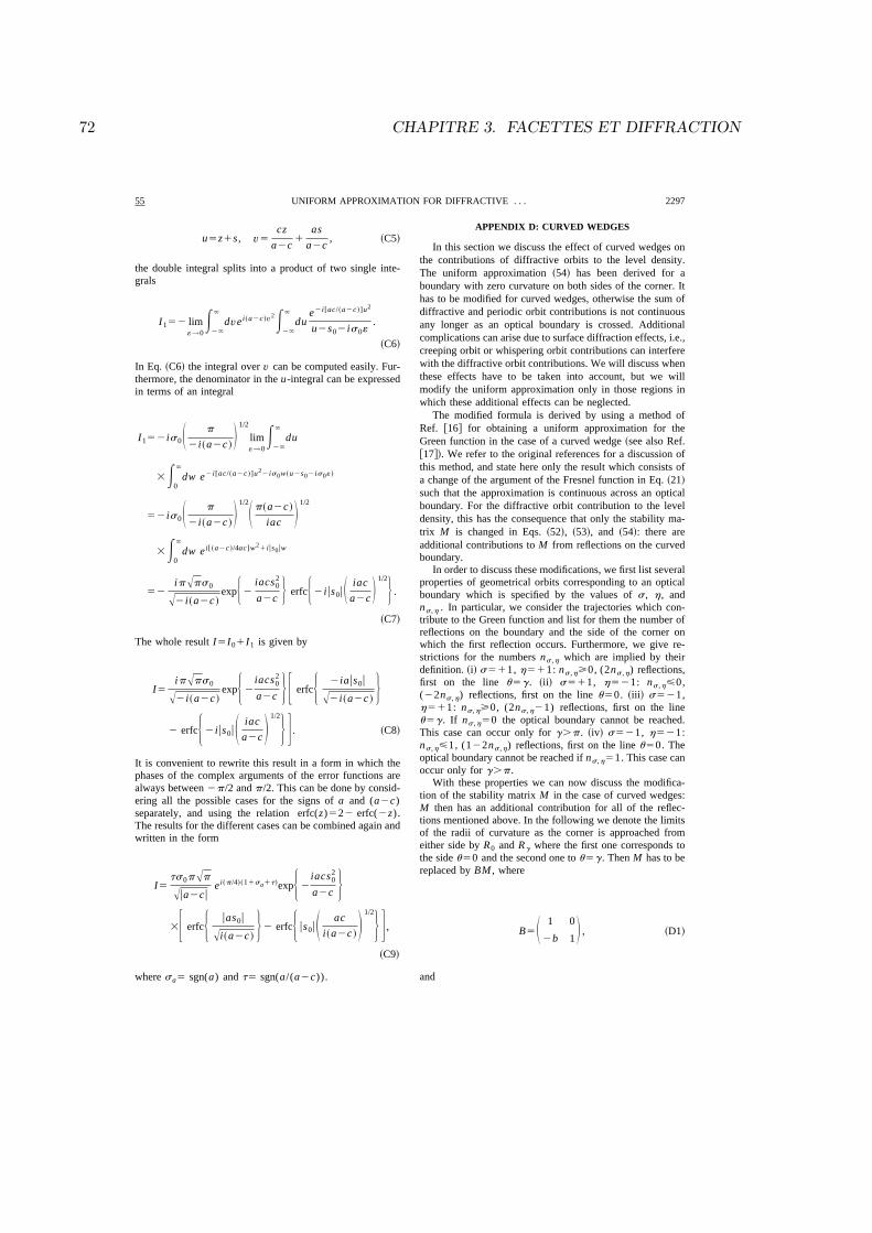
72 CHAPITRE 3. FACETTES ET DIFFRACTION
u5z1s , v5
cz
a2c1
as
a2c, ~C5!
the double integral splits into a product of two single inte-grals
I152 lim«→0
E2`
`
dve i~a2c !v2E2`
`
due2i[ac/~a2c !]u2
u2s02is0«.
~C6!
In Eq. ~C6! the integral over v can be computed easily. Fur-thermore, the denominator in the u-integral can be expressedin terms of an integral
I152is0S p
2i~a2c !D 1/2 lim
«→0E
2`
`
du
3E0
`
dw e2i[ac/~a2c !]u22is0w~u2s02is0« !
52is0S p
2i~a2c !D 1/2S p~a2c !
iac D 1/2
3E0
`
dw e i[~a2c !/4ac]w21ius0uw
52
ipAps0
A2i~a2c !expH 2
iacs02
a2c J erfcH 2ius0uS iaca2c D1/2J .~C7!
The whole result I5I01I1 is given by
I5ipAps0
A2i~a2c !expH 2
iacs02
a2c J F erfcH 2iaus0u
A2i~a2c !J
2 erfcH 2ius0uS iaca2c D1/2J G . ~C8!
It is convenient to rewrite this result in a form in which thephases of the complex arguments of the error functions arealways between 2p/2 and p/2. This can be done by consid-ering all the possible cases for the signs of a and (a2c)separately, and using the relation erfc(z)522 erfc(2z).The results for the different cases can be combined again andwritten in the form
I5ts0pAp
Aua2cue i~p/4!~11sa1t !expH 2
iacs02
a2c J3F erfcH uas0u
Ai~a2c !J 2 erfcH us0uS ac
i~a2c !D1/2J G ,
~C9!
where sa5 sgn(a) and t5 sgn(a/(a2c)).
APPENDIX D: CURVED WEDGES
In this section we discuss the effect of curved wedges onthe contributions of diffractive orbits to the level density.The uniform approximation ~54! has been derived for aboundary with zero curvature on both sides of the corner. Ithas to be modified for curved wedges, otherwise the sum ofdiffractive and periodic orbit contributions is not continuousany longer as an optical boundary is crossed. Additionalcomplications can arise due to surface diffraction effects, i.e.,creeping orbit or whispering orbit contributions can interferewith the diffractive orbit contributions. We will discuss whenthese effects have to be taken into account, but we willmodify the uniform approximation only in those regions inwhich these additional effects can be neglected.
The modified formula is derived by using a method ofRef. @16# for obtaining a uniform approximation for theGreen function in the case of a curved wedge ~see also Ref.@17#!. We refer to the original references for a discussion ofthis method, and state here only the result which consists ofa change of the argument of the Fresnel function in Eq. ~21!such that the approximation is continuous across an opticalboundary. For the diffractive orbit contribution to the leveldensity, this has the consequence that only the stability ma-trix M is changed in Eqs. ~52!, ~53!, and ~54!: there areadditional contributions to M from reflections on the curvedboundary.
In order to discuss these modifications, we first list severalproperties of geometrical orbits corresponding to an opticalboundary which is specified by the values of s , h , andns ,h . In particular, we consider the trajectories which con-tribute to the Green function and list for them the number ofreflections on the boundary and the side of the corner onwhich the first reflection occurs. Furthermore, we give re-strictions for the numbers ns ,h which are implied by theirdefinition. ~i! s511, h511: ns ,h>0, (2ns ,h) reflections,first on the line u5g . ~ii! s511, h521: ns ,h<0,(22ns ,h) reflections, first on the line u50. ~iii! s521,h511: ns ,h>0, (2ns ,h21) reflections, first on the lineu5g . If ns ,h50 the optical boundary cannot be reached.This case can occur only for g.p . ~iv! s521, h521:ns ,h<1, (122ns ,h) reflections, first on the line u50. Theoptical boundary cannot be reached if ns ,h51. This case canoccur only for g.p .
With these properties we can now discuss the modifica-tion of the stability matrix M in the case of curved wedges:M then has an additional contribution for all of the reflec-tions mentioned above. In the following we denote the limitsof the radii of curvature as the corner is approached fromeither side by R0 and Rg where the first one corresponds tothe side u50 and the second one to u5g . Then M has to bereplaced by BM , where
B5S 1 0
2b 1 D , ~D1!
and
55 2297UNIFORM APPROXIMATION FOR DIFFRACTIVE . . .

3.3. DIFFRACTION 73
This approximation is only valid as long as all sine functionsin Eq. ~D2! are positive and not close to zero. The case of analmost vanishing sine function corresponds to near grazingincidence on a side of the corner. Then surface diffractioneffects become important and interfere with the diffractiveorbit contribution, and the uniform approximation is nolonger valid. In the case that some sine functions are nega-tive and not small, the orbit is not close to an optical bound-ary and the GTD approximation can be used ~it is the sameas in the case of non-curved wedges!.
There is a disadvantage of the definition of B givenabove. Since there are two possibilities for choosing u1 andu2 corresponding to the two arms of a diffractive orbit in acorner, it follows from Eq. ~D2! that the uniform approxima-tion is not uniquely defined. ~Note that both cases have to be
checked for deciding whether surface diffraction effects areimportant.!
The nonuniqueness of the approximation is a direct con-sequence of the fact that the uniform approximation for theGreen function of Ref. @16# is not symmetric underu1↔u2. It is another example for the nonuniqueness of uni-form approximations ~cf. the discussion in Sec. II C!. How-ever, as an optical boundary is approached, both choices givethe same result as they should. Let us discuss in more detailthe difference between these two choices. It can be shownthat interchanging u1 and u2 amounts to evaluate Eq. ~D2!with u15su212ns ,hg2hp instead of u1. This then di-rectly suggests a possible way by which this ambiguity canbe removed, namely, by replacing u1 in Eq. ~D2! by theaverage of both values which is (u11su212ns ,hg2hp)/2. As an optical boundary is approached,this combination again becomes identical to u1.
@1# M. C. Gutzwiller, Chaos in Classical and Quantum Mechanics~Springer-Verlag, New York, 1990!.
@2# R. Balian and C. Bloch, Ann. Phys. ~N.Y.! 60, 401 ~1970!.@3# R. Balian and C. Bloch, Ann. Phys. ~N.Y.! 69, 76 ~1972!.@4# G. Vattay, A. Wirzba, and P. E. Rosenqvist, Phys. Rev. Lett.
73, 2304 ~1994!; G. Vattay, A. Wirzba, and P. E. Rosenqvist,in Proceedings of the International Conference on DynamicalSystems and Chaos, Tokyo, edited by Y. Aizawa, S. Saito, andK. Shiraiwa ~World Scientific, Singapore, 1995!, p. 463; P. E.Rosenqvist, G. Vattay, and A. Wirzba, J. Stat. Phys. 83, 243~1996!.
@5# N. D. Whelan, Phys. Rev. E 51, 3778 ~1995!.@6# N. Pavloff and C. Schmit, Phys. Rev. Lett. 75, 61 ~1995!; 75,
3779~E! ~1995!.@7# H. Primack, H. Schanz, U. Smilansky, and I. Ussishkin, Phys.
Rev. Lett. 76, 1615 ~1996!.@8# H. Bruus and N. D. Whelan, Nonlinearity 9, 1023 ~1996!.@9# J. B. Keller, J. Opt. Soc. Am. 52, 116 ~1962!.
@10# W. Pauli, Phys. Rev. 54, 924 ~1938!.@11# R. M. Lewis and J. Boersma, J. Math. Phys. 10, 2291 ~1969!.@12# D. S. Ahluwalia, R. M. Lewis, and J. Boersma, SIAM J. Appl.
Math. 16, 783 ~1968!.@13# D. S. Ahluwalia, SIAM J. Appl. Math. 18, 287 ~1970!.@14# S.-W. Lee and G. A. Deschamps, IEEE Trans. Antennas
Propag. AP-24, 25 ~1976!.
@15# P. C. Clemmow, Q. J. Mech. Appl. Math. 3, 241 ~1950!.@16# R. G. Kouyoumjian and P. H. Pathak, Proc. IEEE 62, 1448
~1974!.@17# G. L. James, Geometrical Theory of Diffraction for Electro-
magnetic Waves ~Peregrinus, Stevenage, England, 1976!.@18# J. Boersma, Q. J. Mech. Appl. Math. 28, 405 ~1975!.@19# S. W. Lee and J. Boersma, J. Math. Phys. 16, 1746 ~1975!.@20# R. Mittra and Y. Rahmat-Samii, in Electromagnetic Scatter-
ing, edited by P.L.E. Uslenghi ~Academic, New York, 1978!,p. 121.
@21# M. Schneider and R. J. Luebbers, IEEE Trans. AntennasPropag. AP-39, 8 ~1991!.
@22# A. Sommerfeld, Optics ~Academic, New York, 1954!.@23# H. S. Carslaw, Proc. London Math. Soc. Ser. 1 30, 121 ~1899!.@24# H. S. Carslaw, Proc. London Math. Soc. Ser. 2 18, 291 ~1920!.@25# Handbook of Mathematical Functions, edited by M.
Abramowitz and I. A. Stegun ~Dover, New York, 1972!.@26# M. V. Berry and M. Wilkinson, Proc. R. Soc. London Ser. A
392, 15 ~1984!.@27# E. B. Bogomolny, Nonlinearity 5, 805 ~1992!.@28# T. Harayama and A. Shudo, Phys. Lett. A 165, 417 ~1992!.@29# P. A. Boasman, Nonlinearity 7, 485 ~1994!.@30# D. Alonso and P. Gaspard, J. Phys. A 27, 1599 ~1994!.@31# B. Georgeot and R. E. Prange, Phys. Rev. Lett. 74, 2851
2298 55MARTIN SIEBER, NICOLAS PAVLOFF, AND CHARLES SCHMIT
74 CHAPITRE 3. FACETTES ET DIFFRACTION
~1995!.@32# B. Burmeister and F. Steiner ~unpublished!.@33# C. Pisani, Ann. Phys. 251, 208 ~1996!.@34# C. Schmit, in Chaos and Quantum Mechanics, edited by M.-J.
Giannoni, A. Voros, and J. Zinn-Justin, Les Houches Summer-
School Lectures LII, 1989 ~North-Holland, Amsterdam, 1991!,p. 331.
@35# S. C. Creagh, J. M. Robbins, and R. G. Littlejohn, Phys. Rev.A 42, 1907 ~1990!.
@36# T. Hesse ~unpublished!.
55 2299UNIFORM APPROXIMATION FOR DIFFRACTIVE . . .
Chapitre 4
Effets de couche et rugosite
4.1 Presentation
La formation de facettes qui a ete presentee au chapitre precedent est un effet qui va au-deladu modele de gelee (ce modele a ete presente au premier chapitre). C’est une consequence du ca-ractere discret de la structure ionique sous-jacente. Les facettes peuvent etre considerees commel’apparition dans l’agregat d’un ordre ionique correspondant a une limite de faible temperature1.A relativement haute temperature, l’agitation thermique va detruire l’ordre ionique, sans en-core affecter les couches quantiques et l’on pourrait penser que les ions occupant des positionsquasi-aleatoires, le modele de gelee est alors plus pertinent. Cependant il faut garder a l’es-prit que la vitesse de Fermi des electrons est de plusieurs ordres de grandeur superieure ala vitesse des ions : si l’on estime tres grossierement cette derniere par la vitesse d’agitationthermique d’un gaz parfait classique (ce qui donne une borne superieure de cette vitesse) onobtient < vion >≈ (3kBT/mion)1/2 ' 600 m/s pour du sodium a T = 400 K, alors que lavitesse de Fermi electronique est vF = (9π/4)1/3h/(me rS) ' 106 m/s (rS = 2.08 A est le rayonde Wigner-Seitz du sodium). Donc les electrons “voient” des ions quasiment immobiles, memedans la limite des temperatures elevees (mais dans cette limite l’arrangement des ions dans l’es-pace est quasi-aleatoire). On a vu, dans le chapitre 1, que les electrons de valence des metauxalcalins etaient peu sensibles a l’arrangement du reseau ionique (section 1.2). Donc le desordreionique affectera peu la densite electronique a l’interieur de l’agregat (loin de la surface). Enrevanche, il est clair que la forme du champ moyen en surface depend de l’ordre (ou du desordre)ionique2 et que cela a une incidence importante sur les niveaux quantiques : l’effet de couchen’est pas le meme dans une sphere et dans un patatoıde bossele. Donc la nature discrete de lastructure ionique sous-jacente a un effet sur la structure electronique de l’agregat, meme avantl’apparition de facettes.
Dans la reference [Pav98] reproduite ci-apres, la deformation de la surface de l’agregatcausee par l’agitation thermique des ions a ete estimee avec un modele de goutte liquide. Dansce modele, la deformation correspond a des ondes capillaires excitees thermiquement. L’agregatest considere comme globalement spherique, avec des ecarts a la sphericite caracterises par unelongueur typique ∆ de la forme ∆ ∝
√
kBT/σ ou σ est la tension superficielle du materiau (il y
1Ainsi, suivant les conditions experimentales de temperature, on peut voir des agregats de meme taille (N '
2000), formes du meme element (le sodium), exhiber des effets de couche quantiques (ref. [Ped91]) ou geometriques(ref. [Mar90]).
2Le cas extreme etant celui de l’agregat facette, le champ moyen a dans ce cas une forme tout a fait nonspherique.
75
76 CHAPITRE 4. EFFETS DE COUCHE ET RUGOSITE
a egalement une faible variation de ∆ avec la taille de l’agregat, cf. [Pav98]). Ensuite, la densitede niveaux et la partie oscillante de l’energie electronique sont obtenues a partir d’une formuledes traces qui prend en compte les effets de desordre de la surface et qui a ete derivee dans la ref.[Pav95a] (reproduite ci-apres). Les calculs se comparent bien avec les resultats experimentauxdu groupe de S. Bjørnholm [Cha97] sur les agregats de sodium de taille 50 ≤ N ≤ 250 (cf. lafigure 4.2 ci-dessous).
Cette approche (dont la motivation physique vient d’etre presentee) ne correspond pas al’interpretation des causes de deformation generalement admise dans le domaine des agregatsmetalliques. Ce sont les effets de couche electroniques qui sont le plus souvent invoques pourexpliquer la deformation des agregats. Ce type de deformation est analogue aux deformations deJahn-Teller [Jah37] : entre deux nombres magiques (en “milieu de couche”) il y a un maximumlocal de la partie oscillante de l’energie electronique totale (on note Eshell cette energie et onl’appelle energie de couche, cf. figure 2.5). En brisant la symetrie spherique, on fait decroıtreEshell et on gagne donc de l’energie d’origine quantique. Bien sur, on perd egalement de l’energiede surface en deformant la sphere, mais jusqu’a des tailles relativement elevees, c’est le gain enenergie de couche qui domine.
Ce type d’interpretation a motive plusieurs etudes theoriques des effets de deformationutilisant differents types de description des agregats. Des approches basees sur l’approximationde gelee traitee par la methode de la fonctionnelle de la densite ont donne un accord semi-quanti-tatif avec les observations experimentales pour des taillesN <∼ 100 [Eka88, Hir94, Kos95, Mon95].Dans cette gamme de taille, il se trouve que des modeles plus simples ont obtenu de meilleursresultats. Ainsi, Yannouleas et Landman [Yan95, Yan96, Yan97] ont assis l’interpretation ala Jahn-Teller des effets de deformation en utilisant un modele de champ moyen non auto-consistant (oscilateur harmonique deforme), couple par la methode des corrections de couche aun modele de goutte liquide. Ils ont effectue une etude systematique des potentiels d’ionisation,des affinites electroniques et des energies de dissociation des agregats de sodium, potassiumet lithium et ont pu reproduire quantitativement une vaste gamme de donnees experimentalesdans le regime des tailles N <∼ 100.
Pour les tailles plus elevees, le mecanisme invoque reste le meme, et plusieurs auteurs [Bul93,Rei93, Fra96b] ont etudie la deformation des agregats jusqu’a des tailles de l’ordre de N ∼ 1000en utilisant des potentiels empiriques pour decrire le champ moyen electronique, dans un cadresimilaire a celui employe avec succes par Yannouleas et Landman pour des tailles moins elevees.Les conclusions obtenues sont toutes similaires et illustrees par la figure 4.1(b) ci-dessous quireproduit les resultats de Frauendorf et Pashkevich [Fra96a] : les agregats sont deformes en milieude couche et spheriques pres des nombres magiques (pres des “fermetures de couche”). L’allurequalitative des resultats pour l’energie de couche Eshell obtenue dans ces travaux se discutesimplement grace a une approche semiclassique : ainsi, afin d’illustrer l’interet energetique d’unedeformation en milieu de couche, on peut estimer, pour un systeme chaotique, integrable ou asymetrie spherique, l’ordre de grandeur des termes oscillants dans la densite de niveaux et endeduire la dependance en N de l’energie de couche. C’est ce qui est schematiquement representedans le tableau synoptique 4.1 pour le cas d’un billard tridimensionnel, L etant une grandeurtypique du billard (proportionnelle a rS N
1/3).
On constate sur la table 4.1 que deformer la sphere pour en faire un billard chaotique faitquasiment disparaıtre les effets de couche. Donc, pres d’une fermeture de couche, lorsque Eshell
est negative dans la sphere, la forme spherique est favorisee. En milieu de couche au contraire,Eshell est positive dans la sphere (cf. fig. 2.5) et cela conduit a des deformations. L’allure typiquedu graphe donnant Eshell en fonction de la taille N de l’agregat est donc le suivant : des minima
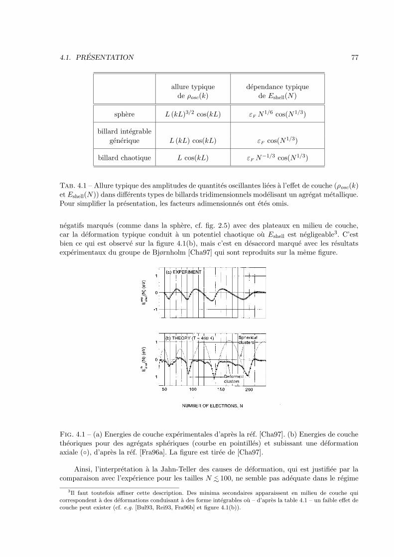
4.1. PRESENTATION 77
allure typique dependance typiquede ρosc(k) de Eshell(N)
sphere L (kL)3/2 cos(kL) εF N1/6 cos(N1/3)
billard integrable
generique L (kL) cos(kL) εF cos(N1/3)
billard chaotique L cos(kL) εF N−1/3 cos(N1/3)
Tab. 4.1 – Allure typique des amplitudes de quantites oscillantes liees a l’effet de couche (ρosc(k)et Eshell(N)) dans differents types de billards tridimensionnels modelisant un agregat metallique.Pour simplifier la presentation, les facteurs adimensionnes ont etes omis.
negatifs marques (comme dans la sphere, cf. fig. 2.5) avec des plateaux en milieu de couche,car la deformation typique conduit a un potentiel chaotique ou Eshell est negligeable3. C’estbien ce qui est observe sur la figure 4.1(b), mais c’est en desaccord marque avec les resultatsexperimentaux du groupe de Bjørnholm [Cha97] qui sont reproduits sur la meme figure.
Fig. 4.1 – (a) Energies de couche experimentales d’apres la ref. [Cha97]. (b) Energies de couchetheoriques pour des agregats spheriques (courbe en pointilles) et subissant une deformationaxiale (◦), d’apres la ref. [Fra96a]. La figure est tiree de [Cha97].
Ainsi, l’interpretation a la Jahn-Teller des causes de deformation, qui est justifiee par lacomparaison avec l’experience pour les tailles N <∼ 100, ne semble pas adequate dans le regime
3Il faut toutefois affiner cette description. Des minima secondaires apparaissent en milieu de couche quicorrespondent a des deformations conduisant a des forme integrables ou – d’apres la table 4.1 – un faible effet decouche peut exister (cf. e.g. [Bul93, Rei93, Fra96b] et figure 4.1(b)).

78 CHAPITRE 4. EFFETS DE COUCHE ET RUGOSITE
des tailles elevees. Il se trouve que l’approche concurrente, que nous avons exposee en debutde chapitre, conduit a un accord avec l’experience bien meilleur dans ce regime de taille, c’estillustre par la figure 4.2. Ce point est discute en detail dans l’article [Pav98] ci-dessous ou nousarrivons a la conclusion que, dans le regime des grandes tailles, le mecanisme de Jahn-Teller estloin de jouer le role exclusif qu’il semble avoir pour les faibles tailles4. On a reproduit avant cetarticle une reference anterieure [Pav95a] ou est derivee une formule des traces dans un billardrugeux qui est ensuite utilisee pour la discussion des effets de couche dans [Pav98].
Fig. 4.2 – Comparaison entre les energies de couche experimentales obtenues dans la ref. [Cha97](•) et les resultats du modele de billard rugueux de [Pav98] (courbe en trait plein). Les calculstheoriques correspondent a une temperature T = 300 K choisie pour avoir un bon accord avecl’experience (cf. la discussion dans la ref. [Pav98]).
Pour terminer cette presentation, remarquons que la vieille image d’un spectre aleatoire(due a Kubo, cf. section 1.1) et les modeles modernes d’electrons delocalises dans un champmoyen sans desordre semblent contradictoires. Ainsi, dans leur article de 1965, Gor’kov etEliashberg affirment “the distribution of the levels should be random even if the particles havethe same volume and a good shape, say spherical particles of equal size. The point is thatelectrons in the metal have a wavelength of the order of atomic dimensions. Therefore surfaceirregularities of atomic size are sufficient to make the level distribution perfectly random”.Cependant, c’est un fait experimental que les effets de couche existent malgre le desordre desurface. Au vu de la citation ci-dessus cela peut sembler paradoxal et un des buts des refs.[Pav95a, Pav98] est de concilier les deux approches en donnant une description semiclassiquede la structure en couche en presence de desordre a la surface.
4.2 Articles
4.2.1 “Trace formula for an ensemble of bumpy billiards” (ref. [Pav95a])
4Il faut noter que la predominance du mecanisme de Jahn-Teller avait deja ete partiellement remise en questiondans le regime des faibles tailles. Les auteurs de la reference [Aku95] decrivent le systeme d’electrons en interactionmutuelle et en interaction avec le fond ionique par un potentiel de champ moyen auquel se rajoute un hamiltonienaleatoire. L’amplitude de la perturbation aleatoire est fixee d’une part par la temperature et aussi partiellementpar minimisation de l’energie de l’agregat (pour decrire le phenomene de Jahn-Teller). Les resultats obtenus sonten tres bon accord avec les energies de dissociation experimentales du lithium, du sodium et du potassium.

4.2. ARTICLES 79
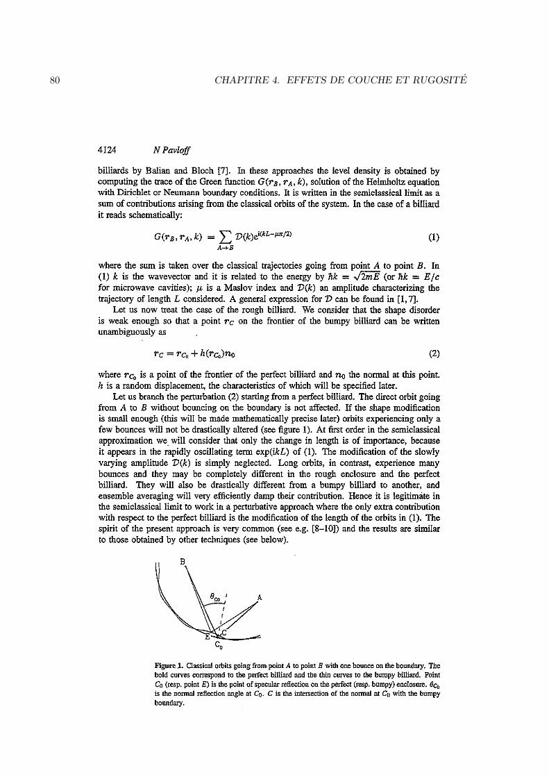
80 CHAPITRE 4. EFFETS DE COUCHE ET RUGOSITE
4.2. ARTICLES 81

82 CHAPITRE 4. EFFETS DE COUCHE ET RUGOSITE

4.2. ARTICLES 83
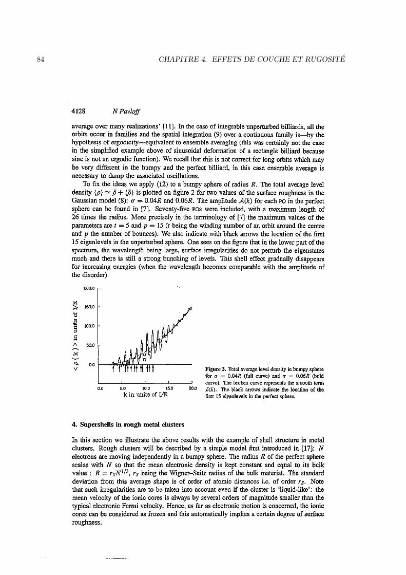
84 CHAPITRE 4. EFFETS DE COUCHE ET RUGOSITE

4.2. ARTICLES 85
86 CHAPITRE 4. EFFETS DE COUCHE ET RUGOSITE

4.2. ARTICLES 87

88 CHAPITRE 4. EFFETS DE COUCHE ET RUGOSITE
4.2. ARTICLES 89
4.2.2 “Rough droplet model for spherical metal clusters” (ref. [Pav98])

90 CHAPITRE 4. EFFETS DE COUCHE ET RUGOSITE
Rough droplet model for spherical metal clusters
Nicolas Pavloff and Charles SchmitDivision de Physique Theorique, Institut de Physique Nucleaire, F-91406 Orsay Cedex, France
~Received 29 September 1997; revised manuscript received 1 April 1998!
We study the thermally activated oscillations, or capillary waves, of a neutral metal cluster within the liquiddrop model. These deformations correspond to a surface roughness which we characterize by a single para-meter D . We derive a simple analytic approximate expression determining D as a function of temperature andcluster size. We then estimate the induced effects on shell structure by means of a periodic orbit analysis, andcompare with recent data for shell energy of sodium clusters in the size range 50,N,250. A small surfaceroughness D.0.6 Å is seen to give a reasonable account of the decrease of amplitude of the shell structureobserved in experiment. Moreover—contrary to usual Jahn-Teller-type of deformations—roughness correctlyreproduces the shape of the shell energy in the domain of sizes considered in experiment.@S0163-1829~98!05328-4#
I. INTRODUCTION
Since the discovery of shell effects in metal clusters, themean-field approach with delocalized electrons has been avery efficient tool for describing a wide variety of phenom-ena: shell and supershell effects, dipole polarizability andoptical excitations, fission, etc. ~for reviews, see Refs. 1 and2!. This type of approach mainly relies on the jellium model,where the ionic background is considered as a smooth anduniform distribution of positive charges. It is most legitimatefor simple metals ~and to a lesser extent for noble metals!with delocalized valence electrons, almost insensitive to theactual arrangement of the ionic cores. Hence the best candi-dates for this approximation are the alkali metals, as can beinferred from the quasisphericity of their Fermi surface ~re-vealing a weak interaction between ionic cores and valenceelectrons!. As a result the compressibility of these solids isclose to its electron gas value, and the surface tension iscorrectly described by the jellium models ~the agreement be-ing better for small electronic density; see Ref. 3!.
It was realized early that deformation effects had to betaken into account for a realistic description of metal clusters~see, e.g., Ref. 4!. Within density-functional theories, thiscan be achieved by imposing to the jellium the shape thatsuits the electrons best.5–7 Deformations have also been stud-ied in less elaborate models ~deformed external meanfield!,8–13 and there is a good overall agreement with experi-mental data for ionization potentials, dissociation energies,and splitting of dipole resonances for relatively small clus-ters ~less than 40 atoms!.
The above-mentioned deformations are of Jahn-Tellertype, and occur between major shell closures, where lower-ing the symmetry leads to a gain in energy. Another type ofsurface deformation also has to be considered which consistsof surface irregularities of very large multipolarities. Thesedeformations not only lower the shell effect, but also intro-duce randomness into the spectrum. This was first noticed byGor’kov and Eliashberg,14 who claimed that ‘‘the distribu-tion of the levels should be random even if the particles havethe same volume and a good shape, say spherical particles ofequal size. The point is that electrons in the metal have a
wavelength of the order of atomic dimensions. Thereforesurface irregularities of atomic size are sufficient to make thelevel distribution perfectly random.’’ This statement has tobe tempered in view of the success of the jellium model.Nevertheless it leaves no doubt that the surface of a clusterhas atomic size irregularities; it is now important to estimatetheir amplitude and to evaluate the resulting effect on thephysical observables.
The fact that disorder is located on the surface is legiti-mated because the elastic mean free path of an electron in thebulk is typically of order of several hundreds of Å, whereasan electron experiences collisions on the surface of the clus-ter about each 10 Å. Indeed, it was shown in Ref. 15 that thescattering of electrons on the fluctuation of the positive ionshas an effect of the same order as that of the thermal distri-bution of the occupancy probability, which in turn is shownin the present work to be negligible compared to the effect ofshape fluctuations. More microscopically, bulk disorderwould be represented by fluctuations of the bottom of thepotential well, and in the large-size limit high-lying statestend to be insensitive to this perturbation, whereas the effectsof surface disorder increase when one goes up in thespectrum.16 Note that such irregularities are also to be takeninto account when the cluster is ‘‘liquidlike’’: the mean ve-locity of the ionic cores is always smaller by several ordersof magnitude than the typical electronic Fermi velocity.Hence, as far as electronic motion is concerned, the ioniccores can be considered as frozen, and this necessarily im-plies a certain degree of surface roughness.
In the present paper we use a liquid drop model to studythe thermally activated surface deformations, or capillarywaves, of a neutral spherical cluster ~Sec. II!. These defor-mations correspond to a surface roughness, which we char-acterize by a single parameter D . We derive a simple analyticapproximate expression determining the behavior of D as afunction of temperature and cluster size. Then in Sec. III wediscuss the influence of shape fluctuations on the level den-sity using a trace formula in rough billiards, and comparewith thermal effects linked with the Fermi occupation num-ber of the energy levels ~for this purpose we give the generalform of shell corrections in the presence of temperature in
PHYSICAL REVIEW B 15 AUGUST 1998-IIVOLUME 58, NUMBER 8
PRB 580163-1829/98/58~8!/4942~10!/$15.00 4942 © 1998 The American Physical Society
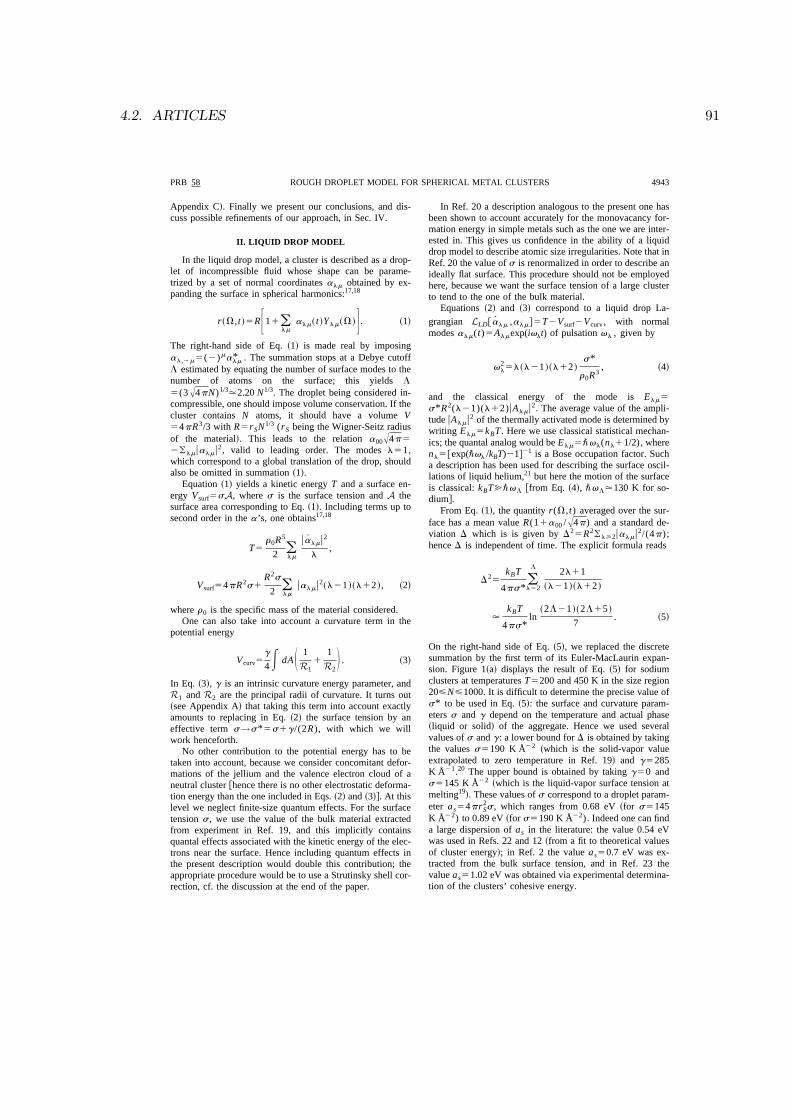
4.2. ARTICLES 91
Appendix C!. Finally we present our conclusions, and dis-cuss possible refinements of our approach, in Sec. IV.
II. LIQUID DROP MODEL
In the liquid drop model, a cluster is described as a drop-let of incompressible fluid whose shape can be parame-trized by a set of normal coordinates alm obtained by ex-panding the surface in spherical harmonics:17,18
r~V ,t !5RF11(lm
alm~ t !Y lm~V !G . ~1!
The right-hand side of Eq. ~1! is made real by imposingal ,2m5(2)malm* . The summation stops at a Debye cutoffL estimated by equating the number of surface modes to thenumber of atoms on the surface; this yields L
5(3A4pN)1/3.2.20 N1/3. The droplet being considered in-compressible, one should impose volume conservation. If thecluster contains N atoms, it should have a volume V54pR3/3 with R5rSN1/3 (rS being the Wigner-Seitz radiusof the material!. This leads to the relation a00A4p5
2(lmualmu2, valid to leading order. The modes l51,which correspond to a global translation of the drop, shouldalso be omitted in summation ~1!.
Equation ~1! yields a kinetic energy T and a surface en-ergy Vsurf5sA, where s is the surface tension and A thesurface area corresponding to Eq. ~1!. Including terms up tosecond order in the a’s, one obtains17,18
T5
r0R5
2 (lm
ualmu2
l,
Vsurf54pR2s1
R2s
2 (lm
ualmu2~l21 !~l12 !, ~2!
where r0 is the specific mass of the material considered.One can also take into account a curvature term in the
potential energy
Vcurv5g
4E dAS 1
R11
1
R2D . ~3!
In Eq. ~3!, g is an intrinsic curvature energy parameter, andR1 and R2 are the principal radii of curvature. It turns out~see Appendix A! that taking this term into account exactlyamounts to replacing in Eq. ~2! the surface tension by aneffective term s→s*5s1g/(2R), with which we willwork henceforth.
No other contribution to the potential energy has to betaken into account, because we consider concomitant defor-mations of the jellium and the valence electron cloud of aneutral cluster @hence there is no other electrostatic deforma-tion energy than the one included in Eqs. ~2! and ~3!#. At thislevel we neglect finite-size quantum effects. For the surfacetension s , we use the value of the bulk material extractedfrom experiment in Ref. 19, and this implicitly containsquantal effects associated with the kinetic energy of the elec-trons near the surface. Hence including quantum effects inthe present description would double this contribution; theappropriate procedure would be to use a Strutinsky shell cor-rection, cf. the discussion at the end of the paper.
In Ref. 20 a description analogous to the present one hasbeen shown to account accurately for the monovacancy for-mation energy in simple metals such as the one we are inter-ested in. This gives us confidence in the ability of a liquiddrop model to describe atomic size irregularities. Note that inRef. 20 the value of s is renormalized in order to describe anideally flat surface. This procedure should not be employedhere, because we want the surface tension of a large clusterto tend to the one of the bulk material.
Equations ~2! and ~3! correspond to a liquid drop La-grangian LLD@ alm ,alm#5T2Vsurf2Vcurv , with normalmodes alm(t)5Almexp(ivlt) of pulsation vl , given by
vl25l~l21 !~l12 !
s*
r0R3, ~4!
and the classical energy of the mode is Elm5
s*R2(l21)(l12)uAlmu2. The average value of the ampli-tude uAlmu2 of the thermally activated mode is determined bywriting Elm5kBT . Here we use classical statistical mechan-ics; the quantal analog would be Elm5\vl(nl11/2), wherenl5@exp(\vl /kBT)21#21 is a Bose occupation factor. Sucha description has been used for describing the surface oscil-lations of liquid helium,21 but here the motion of the surfaceis classical: kBT@\vL @from Eq. ~4!, \vL.130 K for so-dium#.
From Eq. ~1!, the quantity r(V ,t) averaged over the sur-face has a mean value R(11a00 /A4p) and a standard de-viation D which is is given by D2
5R2(l>2ualmu2/(4p);hence D is independent of time. The explicit formula reads
D25
kBT
4ps*(l52
L2l11
~l21 !~l12 !
.kBT
4ps*ln
~2L21 !~2L15 !
7. ~5!
On the right-hand side of Eq. ~5!, we replaced the discretesummation by the first term of its Euler-MacLaurin expan-sion. Figure 1~a! displays the result of Eq. ~5! for sodiumclusters at temperatures T5200 and 450 K in the size region20<N<1000. It is difficult to determine the precise value ofs* to be used in Eq. ~5!: the surface and curvature param-eters s and g depend on the temperature and actual phase~liquid or solid! of the aggregate. Hence we used severalvalues of s and g: a lower bound for D is obtained by takingthe values s5190 K Å22 ~which is the solid-vapor valueextrapolated to zero temperature in Ref. 19! and g5285K Å21.20 The upper bound is obtained by taking g50 ands5145 K Å22 ~which is the liquid-vapor surface tension atmelting19!. These values of s correspond to a droplet param-eter as54prS
2s , which ranges from 0.68 eV ~for s5145K Å22) to 0.89 eV ~for s5190 K Å22). Indeed one can finda large dispersion of as in the literature: the value 0.54 eVwas used in Refs. 22 and 12 ~from a fit to theoretical valuesof cluster energy!; in Ref. 2 the value as50.7 eV was ex-tracted from the bulk surface tension, and in Ref. 23 thevalue as51.02 eV was obtained via experimental determina-tion of the clusters’ cohesive energy.
PRB 58 4943ROUGH DROPLET MODEL FOR SPHERICAL METAL CLUSTERS
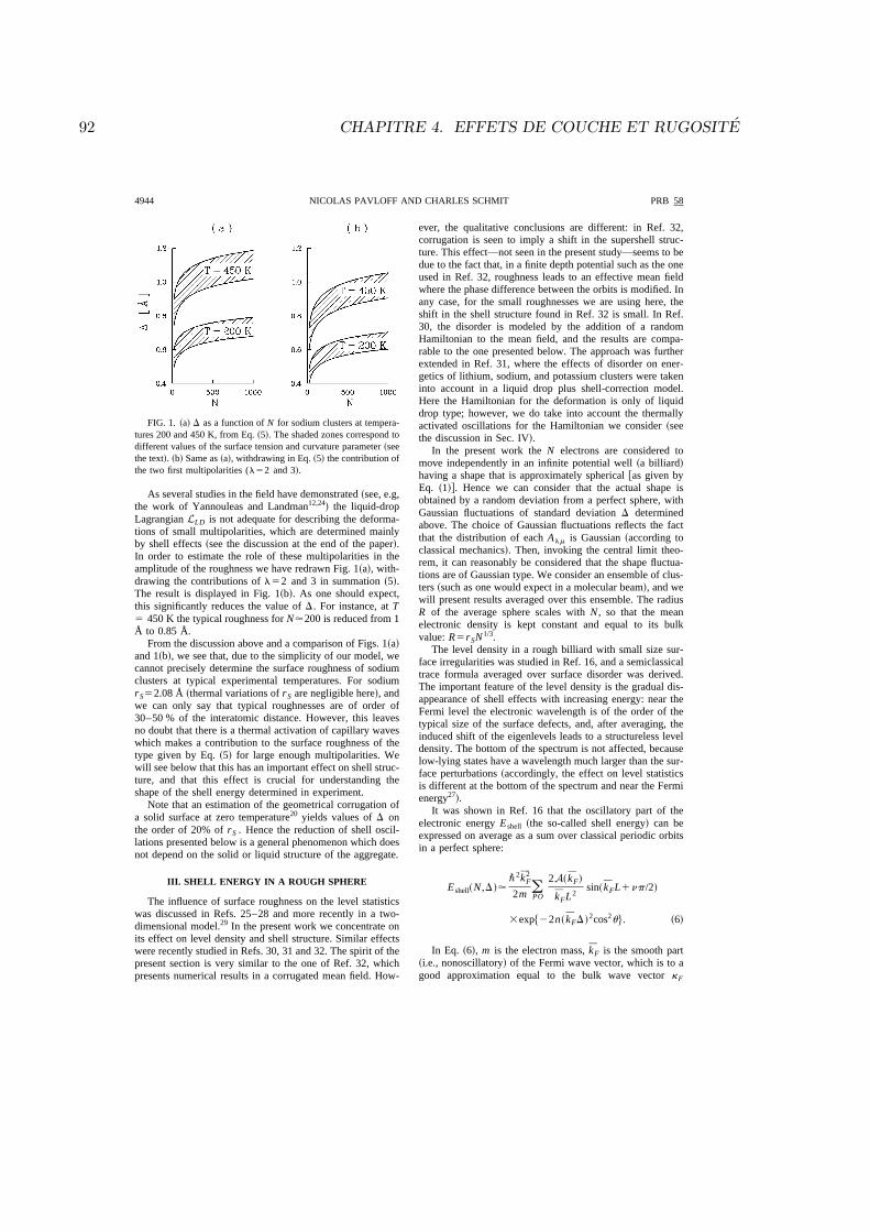
92 CHAPITRE 4. EFFETS DE COUCHE ET RUGOSITE
As several studies in the field have demonstrated ~see, e.g,the work of Yannouleas and Landman12,24! the liquid-dropLagrangian LLD is not adequate for describing the deforma-tions of small multipolarities, which are determined mainlyby shell effects ~see the discussion at the end of the paper!.In order to estimate the role of these multipolarities in theamplitude of the roughness we have redrawn Fig. 1~a!, with-drawing the contributions of l52 and 3 in summation ~5!.The result is displayed in Fig. 1~b!. As one should expect,this significantly reduces the value of D . For instance, at T5 450 K the typical roughness for N.200 is reduced from 1Å to 0.85 Å.
From the discussion above and a comparison of Figs. 1~a!and 1~b!, we see that, due to the simplicity of our model, wecannot precisely determine the surface roughness of sodiumclusters at typical experimental temperatures. For sodiumrS52.08 Å ~thermal variations of rS are negligible here!, andwe can only say that typical roughnesses are of order of30–50 % of the interatomic distance. However, this leavesno doubt that there is a thermal activation of capillary waveswhich makes a contribution to the surface roughness of thetype given by Eq. ~5! for large enough multipolarities. Wewill see below that this has an important effect on shell struc-ture, and that this effect is crucial for understanding theshape of the shell energy determined in experiment.
Note that an estimation of the geometrical corrugation ofa solid surface at zero temperature20 yields values of D onthe order of 20% of rS . Hence the reduction of shell oscil-lations presented below is a general phenomenon which doesnot depend on the solid or liquid structure of the aggregate.
III. SHELL ENERGY IN A ROUGH SPHERE
The influence of surface roughness on the level statisticswas discussed in Refs. 25–28 and more recently in a two-dimensional model.29 In the present work we concentrate onits effect on level density and shell structure. Similar effectswere recently studied in Refs. 30, 31 and 32. The spirit of thepresent section is very similar to the one of Ref. 32, whichpresents numerical results in a corrugated mean field. How-
ever, the qualitative conclusions are different: in Ref. 32,corrugation is seen to imply a shift in the supershell struc-ture. This effect—not seen in the present study—seems to bedue to the fact that, in a finite depth potential such as the oneused in Ref. 32, roughness leads to an effective mean fieldwhere the phase difference between the orbits is modified. Inany case, for the small roughnesses we are using here, theshift in the shell structure found in Ref. 32 is small. In Ref.30, the disorder is modeled by the addition of a randomHamiltonian to the mean field, and the results are compa-rable to the one presented below. The approach was furtherextended in Ref. 31, where the effects of disorder on ener-getics of lithium, sodium, and potassium clusters were takeninto account in a liquid drop plus shell-correction model.Here the Hamiltonian for the deformation is only of liquiddrop type; however, we do take into account the thermallyactivated oscillations for the Hamiltonian we consider ~seethe discussion in Sec. IV!.
In the present work the N electrons are considered tomove independently in an infinite potential well ~a billiard!having a shape that is approximately spherical @as given byEq. ~1!#. Hence we can consider that the actual shape isobtained by a random deviation from a perfect sphere, withGaussian fluctuations of standard deviation D determinedabove. The choice of Gaussian fluctuations reflects the factthat the distribution of each Alm is Gaussian ~according toclassical mechanics!. Then, invoking the central limit theo-rem, it can reasonably be considered that the shape fluctua-tions are of Gaussian type. We consider an ensemble of clus-ters ~such as one would expect in a molecular beam!, and wewill present results averaged over this ensemble. The radiusR of the average sphere scales with N , so that the meanelectronic density is kept constant and equal to its bulkvalue: R5rSN1/3.
The level density in a rough billiard with small size sur-face irregularities was studied in Ref. 16, and a semiclassicaltrace formula averaged over surface disorder was derived.The important feature of the level density is the gradual dis-appearance of shell effects with increasing energy: near theFermi level the electronic wavelength is of the order of thetypical size of the surface defects, and, after averaging, theinduced shift of the eigenlevels leads to a structureless leveldensity. The bottom of the spectrum is not affected, becauselow-lying states have a wavelength much larger than the sur-face perturbations ~accordingly, the effect on level statisticsis different at the bottom of the spectrum and near the Fermienergy27!.
It was shown in Ref. 16 that the oscillatory part of theelectronic energy Eshell ~the so-called shell energy! can beexpressed on average as a sum over classical periodic orbitsin a perfect sphere:
Eshell~N ,D !.\2kF
2
2m (PO
2A~ kF!
kFL2sin~ kFL1np/2!
3exp$22n~ kFD !2cos2u%. ~6!
In Eq. ~6!, m is the electron mass, kF is the smooth part~i.e., nonoscillatory! of the Fermi wave vector, which is to agood approximation equal to the bulk wave vector kF
FIG. 1. ~a! D as a function of N for sodium clusters at tempera-tures 200 and 450 K, from Eq. ~5!. The shaded zones correspond todifferent values of the surface tension and curvature parameter ~seethe text!. ~b! Same as ~a!, withdrawing in Eq. ~5! the contribution ofthe two first multipolarities (l52 and 3!.
4944 PRB 58NICOLAS PAVLOFF AND CHARLES SCHMIT
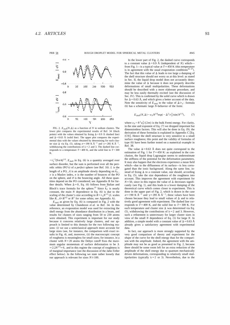
4.2. ARTICLES 93
5rS21(9p/4)1/3. Eshell in Eq. ~6! is a quantity averaged over
surface disorder, but the sum is performed over all the peri-odic orbits ~PO’s! of a perfect sphere ~see Ref. 16!. L is thelength of a PO, A is an amplitude slowly depending on kF ,n is a Maslov index, n is the number of bounces of the POon the sphere, and u is the bouncing angle. All these quan-tities depend on the PO considered; see Appendix B for fur-ther details. When D50, Eq. ~6! follows from Balian andBloch’s trace formula for the sphere.33 Since kF is nearlyconstant, the main N dependence in Eq. ~6! is due to thescaling of the cluster’s size according to R5rSN1/3 (L scaleslike R , A}R5/2 or R2 for some orbits; see Appendix A!.
Eshell as given by Eq. ~6! is compared in Fig. 2 with thevalue determined by Chandezon et al. in Ref. 34. In thisreference, an evaporation model was used for extracting theshell energy from the abundance distribution in a beam, andresults for clusters of sizes ranging from 50 to 230 atomswere obtained. This experiment is important for our studybecause it concerns relatively large clusters, and our ap-proach is limited to this domain for the two following rea-sons: ~i! we use a semiclassical approach more accurate forlarge sizes ~see, for instance, the comparison with exact re-sults in Fig. 4!, and, moreover, ~ii! the macroscopic conceptof roughness is meaningless for small sizes; for instance, in acluster with N520 atoms the Debye cutoff fixes the maxi-mum angular momentum of surface deformation to be L.2.2N1/3.6, and in this regime the concept of roughness isof marginal importance ~see the discussion of the Jahn-Tellereffect below!. In the following we state rather loosely thatour approach is relevant for sizes N*100.
In the lower part of Fig. 2, the dashed curve correspondsto a constant value D50.9 Å ~independent of N) which—from Fig. 1—is a typical value at T5450 K ~this temperatureis in agreement with the usual evaporation conditions35–37!.The fact that this value of D leads to too large a damping ofthe shell structure should not worry us at this level: as statedin Sec. II, the liquid drop model does not accurately deter-mine the value of D because it does not properly describedeformations of small multipolarities. These deformationsshould be described with a more elaborate procedure, andmay be less easily thermally excited ~see the discussion ofSec. IV!. This is confirmed by the solid curve which is drawnfor D50.63 Å, and which gives a better account of the data.Note the sensitivity of Eshell to the value of D/rS : formula~6! has a schematic large N-behavior of the form:
Eshell~N ,D !;«FN1/6exp~2D2/rS2!sin~N1/3!, ~7!
where «F5\2kF2 /(2m) is the bulk Fermi energy. For clarity,
in the sine and exponent of Eq. ~7! we dropped important butdimensionless factors. This will also be done in Eq. ~9!; thederivation of these formulas is explained in Appendix C @Eq.~C9!#. Hence the shell structure is very sensitive to a smallsurface roughness; this point and the validity of formulas oftype ~6! have been further tested on a numerical example inRef. 38.
The value D50.63 Å does not quite correspond to theestimation of Fig. 1 for T5450 K: as explained in the con-clusion, the liquid drop Lagrangian seems to underestimatethe stiffness of the potential for the deformation parameters.It may also happen that the electrons experience a mean fieldwhich—due to the diffuseness of its surface—is less corru-gated than the ionic background. Along the same line, in-stead of fixing D to a constant value, one should, accordingto Eq. ~5!, take the size dependence of the roughness intoaccount. This improves the agreement with experiment forN.50, since in this region the value of D decreases signifi-cantly ~see Fig. 1!, and this leads to a lower damping of thetheoretical curve which comes closer to experiment. This isdone in the upper part of Fig. 2, which is drawn in the cases5190 K Å22 and g5285 K Å21; these values have beenchosen because they lead to small values of D and to rela-tively good agreement with experiment. The dashed line cor-responds to T5400 K, and the solid line to T5300 K. Foreach temperature and cluster size D was determined via Eq.~5!, withdrawing the contributions of l52 and 3. However,such a refinement is unnecessary for larger cluster sizes inview of the small N dependence of Eq. ~5! for large N . Inaddition, a simple model with a constant value of D50.63 Åalready gives a satisfactory agreement with experimentaldata.
In fact, our approach is more strongly supported by thevery good comparison of theory and experiment for theshape of the curve for the shell energy than for the compari-son with the amplitude. Indeed, the agreement with the am-plitude may not be as good as presented in Fig. 2, becausethere should be some room left for an extra reduction of theamplitude of the shell energy due to quantum mechanicallydriven deformations, corresponding to relatively small mul-tipolarities ~typically l52 or 3!. Nevertheless, due to the
FIG. 2. Eshell(N ,D) as a function of N in sodium clusters. Thelower plot compares the experimental results of Ref. 34 ~blackpoints! with the values obtained by fixing D50.9 Å ~dashed line!
and D50.63 Å ~solid line!. The upper plot compares the experi-mental data with the values obtained by determining for each clus-ter size D via Eq. ~5!, taking s5190 K Å22 and g5285 K Å21,withdrawing the contributions of l52 and 3. The dashed line cor-responds to a temperature T5400 K, and the solid line to T5300K.
PRB 58 4945ROUGH DROPLET MODEL FOR SPHERICAL METAL CLUSTERS

94 CHAPITRE 4. EFFETS DE COUCHE ET RUGOSITE
high sensitivity of formula ~6! to small changes of D , we stillcan conclude from Fig. 2 that the typical roughness is oforder of 0.6 Å.
Concerning the shape of the curve, the experimental re-sults of Ref. 34 are surprising, because they are in contradic-tion with the common belief that cluster’s deformations areonly governed by Jahn-Teller effects. For instance, the dis-sociation energies and ionization potentials of simple metalclusters of relatively small sizes are well accounted for bymodels where the Jahn-Teller effect is the only mechanismof deformation12,24 ~the agreement with experiment survivesup to size N;100 for the ionization potentials of potassium;see Ref. 39!. This phenomenon was expected to occur evenfor large values of N; see, e.g., the zero-temperature resultsof Refs. 11, 13, 9, and 10, or the finite temperature results ofRef. 40. In these studies, the deformations occur betweenshell closures, and their main effect is to remove the upperpart of the shell oscillations; the shell energy is predicted tohave sharp negative spikes in the vicinity of the magic num-bers ~these spikes correspond semiclassically to long PO’s!.On the other hand, surface roughness suppresses long PO’s,and reduces shell structure more uniformly, as seen in theexperimental data of Ref. 34. Hence we feel that previoustheoretical approaches overestimate the role of the Jahn-Teller mechanism: the very specific shape of shell energythey predict is not seen in the experiment of Chandezon et al.The comparison between our approach and the experimentalresults for the sizes N*100 firmly establishes that there is aqualitatively important effect of roughness.
On the quantitative level, one can also notice that typicaltheoretical studies overestimate the shell effect for clusters oflarge sizes: compare Fig. 3 of Ref. 34 with similar figures ofRefs. 11, 13, 9, and 10. Temperature effects improve theagreement ~see Ref. 40!, but there is still a mismatch of orderof 40% for the amplitude of shell oscillations ~see Fig. 3 ofRef. 34!, leaving room for improvement due to surfaceroughness.
For further comparison with experimental data, we dis-play in Table I the magic numbers in the region N,1300.The first column shows the D50 results from the semiclas-sical formula ~6!. The second column displays the exact re-sult in the perfect sphere, and merely tests the accuracy ofthe semiclassical periodic orbit expansion used in the firstcolumn. Note that the magic numbers of these two columnsare almost identical to the results of Bulgac andLewenkopf,10 who used a quadrupole deformation of aspherical billiard model within the shell correction method:this is due to the fact that, as stated above, there is no Jahn-Teller deformation at shell closure. In the third column weshow the magic numbers obtained from Eq. ~6! with D50.63 Å. The three first columns compare well with theexperimental ones from Chandezon et al. ~column 4!, androughness has only a small effect on the location of themagic numbers. We still produce these data because theyjustify the billiard model we are using: the magic numbersfrom Table I are in better agreement with experiment thanthe one obtained with harmonic oscillators9,11 or more elabo-rate potentials.13,40 Hence, as far as the phase difference be-tween the contribution of its PO’s to Eq. ~6! is concerned, thebilliard model is presumably close to the experimental situ-ation, since it allows a good prediction of the minima in the
shell energy. However, the electrons are sensitive to a meanfield which—due to the finite range of the electron-ion andelectron-electron interaction—could be less corrugated thanthe ionic background. This would lead to an effective de-crease of D , and may help improve the model by reducingthe importance of the ionic corrugation, leaving some roomfor an extra decrease in amplitude due to deformations ofJahn-Teller type.
Note that in the present treatment the effects of tempera-ture are indirect: although the usual temperatures reached inexperiments are small compared to the Fermi energy ~oneremains in the highly degenerate limit kBT!«F), they aresufficient to induce a disorder of the cluster’s shape whichhas a sizable effect on shell structure. For comparison onecan derive a formula @similar to Eq. ~6!# encompassing theeffect of a Fermi occupation function in the energy levels ofthe electron gas. The free energy F(N ,T) is more appropri-ate than the total energy for evaluating these effects. Indeed,based on Weisskopf’s approach, the electronic contributionto the evaporation rate of a neutral monomer from a clusterof size N can be shown to be approximatively proportional toexp$@F(N)2F(N21)#/kBT%.40,41 The general formula for theoscillating part of the free energy is derived in Appendix C,and in the case of a billiard reads
Fshell~N ,T !.\2km
2
2m (PO
2A~ km!
kmL2sin~ kmL1np/2!F1~ X !,
~8!
where km is the nonoscillatory part of the quantity km definedby m5\2km
2 /2m , m being the chemical potential. Again, km
is to a good approximation equal to the bulk Fermi wavevector kF . X5(p/2)tLkF
2 / km is a dimensionless quantitywhich tends to zero at T50 (t5kBT/«F is the reduced tem-perature!. More precisely, it can be considered as small if thethermal wavelength lT5(2p\2/mkBT)1/2 is large comparedto ArSL (X52p2L/ kmlT
2). F1 is a dimensionless dampingfunction defined in Appendix C @Eq. ~C3!#.
TABLE I. Magic numbers in the perfectly spherical billiard~column 1: PO expansion; column 2: exact results! and in the roughbilliard ~column 3!. Column 4 shows the experimental results ofChandezon et al.
Eq. ~6!,D50
Exact result,D50
Eq. ~6!,D50.63 Å Ref. 34
56 58 56 5892 92 92 92138 138 136 138184 186 190 19262252 254 252 25662336 338 334 33462436 440 430 43062
540/554 542/556 526 54065610/674 612/676 624 64865744/830 748/832 752
908 912 9021070 1074 10821282 1250 1286
4946 PRB 58NICOLAS PAVLOFF AND CHARLES SCHMIT

4.2. ARTICLES 95
In Fig. 3, we compare the effects of a temperature T5
750 K, with those of a constant roughness D50.63 Å. Theshell energy is displayed as a function of N1/3 for sodiumclusters of size N,3400. There is a striking difference withthe N dependence obtained via usual temperature effects onoccupation numbers. As one notices from the figure, rough-ness damps the oscillations in the total energy with an over-all factor @of the type exp(2D2/rS
2); cf. Eq. ~7!# without modi-fying the qualitative features of the supershells, whereastemperature leads to an N-dependent damping of schematicform @cf. Appendix C, Eq. ~C9!#:
Fshell~N ,T !;«FN1/6F1~tN1/3!sin~N1/3! ~9!
@as in Eq. ~7!, we have omitted numerical factors in the sineand F1 function#. Hence the effects of thermal distribution ofoccupation numbers is to wash out the beating pattern of theshell energy by exponentially damping the large N oscilla-tions ~see also Fig. 4!.
Note also the efficiency of a small roughness for dimin-ishing shell effect: for clusters of size 800,N,1200, fromEqs. ~6! and ~8!, one can see, for instance, that the effect ofa small roughness D50.2rS.R/50 on Eshell is similar to theone of a temperature of about 550 K on Fshell . In the range300,N,500 the same roughness corresponds to a tempera-ture T.750 K, and for 50,N,250 it corresponds to T.1000 K ~around N5200) or 1400 K ~around N5100). Asa result, in a range of sizes and temperatures commonlyreached in experiment (N;500 and T;400 K!, the effect ofroughness on shell structure is dominant compared to that ofthermal distribution of occupation numbers. Furthermore, asdiscussed above, it seems from the experimental results ofRef. 34 that in about the same region, Jahn-Teller deforma-tions of small multipolarity play a smaller role in the shapeof the shell energy than predicted by usual theoretical studies~see Fig. 3 of Ref. 34!. Here we present roughness as aconcomitant phenomenon which ~according to comparisonwith the data of Ref. 34! seems more relevant for large clus-ters. As discussed in Sec. IV, both phenomena should betaken into account for a proper description of deformationsof large clusters.
IV. DISCUSSION
One of the original interests of metal clusters was to pro-vide a physical realization of a discrete and random spec-trum. It was long thought that the randomness of the levelswould lead to a structureless level density, and theoreticalworks were mostly devoted to the study of the two-pointform factor of the spectrum.42,43 It is only during the last twodecades that molecular beams have made it possible to workin a regime where the size of the cluster is well defined andsmall compared to the electronic mean free path. In this re-gime one observes shell effects as a result of finite-size quan-tum effects.1,4 Nevertheless the remark of Gor’kov andEliashberg quoted in Sec. I remains valid to some extent, andthe present work aims at reconciling these two views byproviding a semiclassical description of shell structure in thepresence of shape disorder.
The model we have considered is schematic; a moreelaborate procedure would be to design a Lagrangian for thesurface deformation encompassing the effects of shell struc-ture ~in the spirit of Strutinsky shell corrections!:
L5LLD@ alm ,alm#2Eshell@alm# . ~10!
This approach is typical in a study of deformations of finitefermionic systems. It is used for determining the equilibriumshape, i.e., the set of alm minimizing the total potential en-ergy. Between shell closure it leads to a ground state inwhich the equilibrium value of some of the a’s is nonzero~mainly for small l), contrary to what is obtained in Sec. II,where all the a’s are zero at equilibrium. Using the Lagrang-ian ~10! would also modify the stiffness of the potential nearthe minimum ~since a term E shell would be added to thepotential used in Sec. II!.
Following the procedure of the present paper, one shouldgo one step further and study the thermally activated vibra-tions of the normal modes in Hamiltonian ~10!. Hence theusual Jahn-Teller deformations correspond to the first step ofthe procedure just exposed and to a small multipolarity,whereas surface roughness corresponds to the second step~and to large multipolarity!.
It would be of great interest to verify if the agreementobtained in Sec. III with experimental values would persistwhen describing surface oscillations with a Lagrangian suchas L defined in Eq. ~10!. This form of the Lagrangian islegitimated by confrontation with experiments in the smalland intermediate size domains, where it is commonly admit-ted that clusters of size N&100 experience static deforma-tions of small multipolarities.12,24 The success of the presentmodel ~which uses LLD , and does not include such Jahn-Teller deformations! in the size range N*100 might be ex-plained by the decrease of the shell-energy contribution to L
due to an intrinsic roughness of the surface. Schematicallyone might say that there is less difference between a roughsphere and a rough ellipsoid than between a perfect sphereand a perfect ellipsoid. A similar phenomenon explains thedisappearance of Jahn-Teller deformations with increasingtemperature; see Ref. 40, where deformation is seen to besuppressed by thermal fluctuations. Note, however, that thephenomenon predicted in this reference is size dependent,i.e., not uniform for all cluster sizes ~as roughness would be!;see the precise discussion in Ref. 40.
FIG. 3. Eshell ~expressed in eV! as a function of N1/3 in sodiumclusters. The upper plot is obtained by taking a constant roughnessD50.63 Å. The lower plot corresponds to formula ~C8! for a per-fectly spherical aggregate with a temperature t5kBT/«F50.02,i.e., T5750 K.
PRB 58 4947ROUGH DROPLET MODEL FOR SPHERICAL METAL CLUSTERS

96 CHAPITRE 4. EFFETS DE COUCHE ET RUGOSITE
Note, finally, that thermally induced shape fluctuationshave already been investigated in the study of the broadeningof plasma resonances of metal clusters in Refs. 44–47 andvery recently in the study of shell structure for clusters ofsize smaller than N5100.39 The ideas are similar to the oneexposed above; however, the allowed deformations are lim-ited to simple shapes, whereas it has been considered neces-sary in the present work to include deformations of verylarge multipolarities for studying surface roughness.
ACKNOWLEDGMENTS
We thank S. Frauendorf, J. Lerme, and W. Swiatecki forfruitful discussions. We wish also to express our gratitude toS. Bjo”rnholm for his interest in this study, judicious remarks,and inspiring comments. Division de Physique Theorique del’Institut de Physique Nucleaire is unite de recherche desUniversites Paris XI et Paris VI associated with CNRS.
APPENDIX A
In this appendix we compute the curvature energy Vcurv@defined in Eq. ~3!# for a droplet of shape given by Eq. ~1!.This amounts to evaluating the integral C5*dA(1/R111/R2) for a boundary that is approximately spherical. Thiscan be done by noticing that if A is the surface area of agiven boundary, the modification dA caused by an infinitesi-mal displacement of the boundary reads dA5*dA dz(1/R111/R2), where dz is the normal segmentbetween the undeformed boundary and the deformed one~see, e.g., Ref. 48, Chap. VII!. If this modification corre-sponds to a modification of Eq. ~1! by r→r1dr , one cancompute dA and dz in terms of dr . This allows us to writeC in the form
C5E dVK
r H r21K
K1/22
1
sinu]uS r sin u]ur
K1/2 D2
1
sin2u]fS r]fr
K1/2 D J , ~A1!
where K(V)5r21(]ur)2
1(]fr)2/sin2u. Then, writingr(V)5R@11h(V)# and neglecting terms of order greaterthan O(h2), one obtains
C52RE dVH 11h1
1
2~]uh !2
1
1
2 sin2u~]fh !2J 1O~h3!.
~A2!
The surface area can be expressed in a similar manner~see Ref. 48!:
A5E dA5E dVrK1/25R2E dVH ~11h !2
1
1
2~]uh !2
1
1
2 sin2u~]fh !2J 1O~h3!. ~A3!
The condition of volume conservation imposes*dV(11h)2
5*dV(11h)1O(h3). Hence, comparing Eqs.~A2! and ~A3!, one sees that for small deformations the cur-vature integral is proportional to the surface area: C52A/R1O(h3). The corrections are of third order in the deforma-tion, they are given in Ref. 49 ~Chap. 6! for spheroidal andharmonic deformations. Here we are interested only in termsup to order O(h2), thus the curvature energy Vcurv5gC/4 isequal up to a multiplicative constant to the surface termVsurf5sA: Vcurv is formally obtained from Vsurf by replacingthe surface tension s by an effective term g/(2R).
APPENDIX B
In this appendix we briefly present the results of Ref. 33for the level density in the sphere, and we make explicit thedifferent terms appearing in Eq. ~6! for the perfect billiard.The periodic orbits in the sphere are regular polygons indiametral planes. They are labeled by two numbers (n ,t), nbeing the number of sides and t the winding number of theorbit around the center (n>2t). Note that n is here the sameas the number of bouncing points appearing in the main text@Eq. ~6!#. The oscillating part of the level density in thesphere reads
rosc~k !5(t51
1`
(n52t
1`
An ,t~k !sin~kLn ,t1nn ,tp/2!. ~B1!
The shortest orbits are the pendulating orbit (n52, t51), the triangle (n53, t51), and square (n54, t51).The triangle and the square are sufficient to understand thequalitative features of the shell and supershell structure ~see,e.g., Refs. 50 and 51!. Each orbit bounces on the surfacewith a constant normal angle un ,t5(122t/n)p/2, and has alength Ln ,t52nR cos un,t . The pendulating orbit occurs in atwo-parameter family ~the parameters determine the direc-tion of bouncing!, whereas all the other orbits form three-parameter families. Hence the bouncing ball ~with n52t)has to be treated separately. The explicit formulas for A(k)and n in Eqs. ~6! and ~B1! are (t>1)
nn ,t5H 0 if n52t ,
n13/2 if n.2t~B2!
and
An ,t~k !5H 2
dSkR2
ptif n52t
2dS~21 ! tsin~2un ,t!Acos un ,t
pnR~Rk !3/2 if n.2t ,
~B3!
4948 PRB 58NICOLAS PAVLOFF AND CHARLES SCHMIT

4.2. ARTICLES 97
where dS52 is the spin degeneracy.One sees that the amplitude corresponding to the pen-
dulating orbit is proportional to k , whereas the other familieshave a larger weight ~proportional to k3/2). Generally speak-ing, one can show that the contribution of a d-parameterfamily has an extra kd/2 power with respect to that of anisolated orbit.52
APPENDIX C
In this appendix we derive approximate analytical expres-sions for the oscillatory part of the total energy, and of thefree energy at finite temperature. Similar results concerningthe entropy, the free energy, etc. were previously obtained inRefs. 53 and 54. We nevertheless briefly outline the deriva-tion of the formulas because the references just quoted arenot very explicit and difficult to follow. The formulas arederived in the framework of a general PO expansion: thelevel density is noted r(e); it is separated in a smooth termr(e) and an oscillating term rosc(e). In the present work, wedenote all the smooth terms with an upper bar and the oscil-lating terms with a subscript ‘‘osc,’’ except for the oscillat-ing part of the energies which have a subscript ‘‘shell’’ ac-cording to the general convention in the field. rosc(e) issupposed to be of the form
rosc~e !5Re(PO
B~e ! eiS~e !/\, ~C1!
where S(e) is the action of the PO considered. B(e) is anorbit-dependent amplitude which is of order \21 for chaoticsystems, order \22 for typical integrable systems in threedimensions, and order \25/2 for rotationally symmetric sys-tems as the spherical billiard where families of orbits arecharacterized by three parameters.52
We will estimate the asymptotic form of several integrals,all of the same type, and we first display a formula oftenused below. Let g(e) be a slowly varying function of e @asB(e) is supposed to be#, and g8 its first derivative. Let f(e2m)5@11exp$(e2m)/kBT%#21 be the Fermi function, m be-ing the chemical potential. If S(m)@\ , one has
E0
1`
g~e !f~e2m ! e iS~e !/\de
5
\
i
e iS~m !/\
S8~m ! H g~m !F1~X !2
\
i
g8~m !
S8~m !F2~X !
1
\
i
g~m !S9~m !
@S8~m !#2F3~X !1•••J , ~C2!
where the integral has been evaluated by a contour integra-tion in the complex plane ~see, e.g., Ref. 55!. In the evalua-tion of the integral we have neglected the contribution of apart of the contour located on the positive imaginary axis;this is legitimate provided the temperature is small comparedto the Fermi energy ~degenerate Fermi gas approximation!.X5pS8(m)kBT/\ is a dimensionless quantity which can beconsidered as small if the period S8 of the orbit is smallcompared to a characteristic thermal time \/kBT . F1, F2, andF3 are dimensionless damping functions:
F1~X !5
X
sinh X, F2~X !5
X2cosh X
sinh2X,
F3~X !5
X3
sinh3XS 11
sinh2X
2 D . ~C3!
For obtaining the total energy starting from Eq. ~C1!, onefirst determines the chemical potential m through the equalityN5N(m), where N is the number of electrons and N(m)5*r(e)f(e2m)de . Like r(e), N can be separated in asmooth term N ~the Weyl term! plus an oscillating part Nosc .Accordingly, m can be separated in a smooth function of N
plus an oscillating term: m5m1mosc , where N5N(m).Then the total electronic energy is E5*ef(e
2m)r(e)de . It can also be separated into a smooth part E ,and an oscillating part which is denoted Eshell throughout thepaper @more precisely Eshell(N ,T) in the presence of tem-perature#, in accordance with the general notations in thefield. Eshell reads, approximately,
Eshell5E er~e !f~e2m !de2E er~e !f~e2m !de
.E er~e !@f~e2m !2moscf8~e2m !#de
2E er~e !f~e2m !de
5E erosc~e !f~e2m !de1moscmS dN
dm Dm
2moscE ~e2m !r~e !f8~e2m !de . ~C4!
The last term on the right-hand side of Eq. ~C4! is sub-dominant; moreover, it is zero at zero temperature, and hencewe drop it in the following. Then, from Eqs. ~C1! and ~C2!,one obtains
Eshell~N ,T !.2Re(PO
S \
iS8~m !D 2
B~m !F2~ X !e iS~m !/\,
~C5!
where X is computed as X , with m replacing m .The free energy F(N ,T) is a quantity more appropriate
than the total energy to evaluate the effects of electronictemperature on the abundance of clusters in the beam ~seethe discussion in the main text!. It is defined by
F~N ,T !5mN1E0
1`
der~e !F~e2m !,
where
F~e2m !52kBT ln~11e ~m2e !/kBT!. ~C6!
The oscillating part of the free energy is denoted byFshell(N ,T), and can be evaluated similarly to what has beendone in ~C4!. This yields
PRB 58 4949ROUGH DROPLET MODEL FOR SPHERICAL METAL CLUSTERS
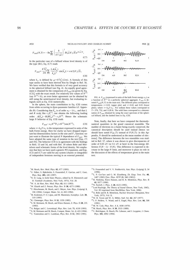
98 CHAPITRE 4. EFFETS DE COUCHE ET RUGOSITE
Fshell~N ,T !.2Re(PO
S \
iS8~m !D 2
B~m !F1~ X !e iS~m !/\,
~C7!
In the particular case of a billiard whose level density is ofthe type ~B1!, Eq. ~C7! reads
Fshell.\2km
2
2m (PO
2A~ km!
kmL2sin~ kmL1np/2!F1~ X !,
~C8!
where km is defined by m5\2km2 /(2m). A formula of this
type seems to have been derived first by Dingle in Ref. 56.We have verified that this formula is of very good accuracyin the spherical billiard ~see Fig. 4!. An equally good agree-ment is obtained for the comparison of Eshell @as given by Eq.~C5!#, with the exact result. For relatively low values of N1/3
~say N1/3,6), an even better agreement can be obtained by
still using the semiclassical level density, but evaluating in-tegrals such as Eq. ~C6! numerically.
In the sphere, the main contribution to Eq. ~C8! comesfrom orbits occurring in three-parameter families ~cf. Appen-dix B!. Considering that km is of order kF;1/rS , and that Land R scale like rSN1/3, one obtains the following leadingorder: A( km);R(Rkm)3/2;rSN5/6. Hence the schematiclarge N behavior of Eq. ~C8! reads
Fshell;«FN1/6F1~tN1/3!sin~N1/3!, ~C9!
where t5kBT/«F is the temperature expressed in units of thebulk Fermi energy. Here for clarity we have dropped impor-tant but dimensionless factors in the sine and F1 function: wejust want to illustrate the typical N dependence of Fshell . Wehave adopted the same type of notation in the text @Eqs. ~7!and ~9!#. The behavior ~C9! is in agreement with the findingsin Refs. 53 and 54, and with Ref. 18 where Bohr and Mot-telson used schematic forms of the level density. We empha-size that here we have used a generic PO expansion, and Eqs.~C5! and ~C7! are valid for any system ~chaotic or integrable!of independent fermions moving in an external potential.
Note, finally, that here we have computed the thermody-namical quantities in the grand canonical ensemble. Thenumber of electrons in a cluster being exactly conserved, thecanonical description should be used instead @hence weshould have noted F(m ,T) instead of F(N ,T): in this Ap-pendix, N should be understood as the mean number of elec-trons#. The difference between the two ensembles was stud-ied in Ref. 57, where it was shown to give discrepancies oforder of 0.05 eV ~or 0.1 eV at best! in the free-energy dif-ference F(N21)2F(N). This difference is expected to de-crease in the large-N limit, and moreover it plays no role inthe discussion of the effects of temperature given in the maintext.
1 M. Brack, Rev. Mod. Phys. 65, 677 ~1993!.2 U. Naher, S. Bjo”rnholm, S. Frauendorf, F. Garcias, and C. Guet,
Phys. Rep. 285, 245 ~1997!.3 N. D. Lang, in Solid State Physics, edited by H. Ehrenreich and
D. Turnbull ~Academic, New York, 1973!, Vol. 28.4 W. A. de Heer, Rev. Mod. Phys. 65, 611 ~1993!.5 W. Ekardt and Z. Penzar, Phys. Rev. B 38, 4273 ~1988!.6 T. Hirschmann, M. Brack, and J. Meyer, Ann. Phys. ~Leipzig! 3,
336 ~1994!; Comput. Mater. Sci. 2, 450 ~1994!.7 M. Koskinen, P. O. Lipas, and M. Manninen, Europhys. Lett. 30,
519 ~1995!.8 K. Clemenger, Phys. Rev. B 32, 1359 ~1985!.9 S. M. Reimann, M. Brack, and Klavs Hansen, Z. Phys. D 28, 235
~1993!.10 A. Bulgac and C. Lewenkopf, Phys. Rev. Lett. 71, 4130 ~1993!.11 S. M. Reimann and M. Brack, Comput. Mater. Sci. 2, 433 ~1994!.12 C. Yannouleas and U. Landman, Phys. Rev. B 51, 1902 ~1995!.
13 S. Frauendorf and V. V. Pashkevich, Ann. Phys. ~Leipzig! 5, 34~1996!.
14 L. P. Gor’kov and G. M. Eliashberg, Zh. Eksp. Teor. Fiz. 48,1407 ~1965! @Sov. Phys. JETP 21, 940 ~1965!#.
15 H. Nishioka, Klavs Hansen, and B. R. Mottelson, Phys. Rev. B42, 9377 ~1990!.
16 N. Pavloff, J. Phys. A 28, 4123 ~1995!.17 Lord Rayleigh, The Theory of Sound ~Dover, New York, 1945!,
Vol. III ~reprinted from MacMillan, New York, 1896!.18 A. Bohr and B. R. Mottelson, Nuclear Structure ~Benjamin, New
York, 1975!, Vol. II.19 W. R. Tyson and W. A. Miller, Surf. Sci. 62, 267 ~1977!.20 J. P. Perdew, Y. Wand, and E. Engel, Phys. Rev. Lett. 66, 508
~1991!.21 M. W. Cole, Phys. Rev. A 1, 1838 ~1970!.22 M. Brack, Phys. Rev. B 39, 3533 ~1989!.23 C. Brechignac, H. Busch, Ph. Cahuzac, and J. Leygnier, J. Chem.
Phys. 101, 6992 ~1994!.
FIG. 4. Fshell ~expressed in units of the bulk Fermi energy «F) asa function of N1/3 in a perfectly spherical aggregate. Fshell is de-noted Fshell(N ,T) in the main text. The different plots correspond totemperatures t50.01 ~upper plot! and t50.02 and 0.03 ~lowerplots!, where t5kBT/«F . For sodium these values correspond toT5376, 752, and 1128 K. The solid lines correspond to a determi-nation of Fshell obtained by using the exact spectrum of the spheri-cal billiard, and the dashed lines to Eq. ~C8!.
4950 PRB 58NICOLAS PAVLOFF AND CHARLES SCHMIT
4.2. ARTICLES 99
24 C. Yannouleas and U. Landman, J. Chem. Phys. 105, 8734~1996!; 107, 1032 ~1997!.
25 K. F. Ratcliff, in Multivariate Analysis V, edited by P. R. Krish-naiah ~North-Holland, Amsterdam, 1980!, p. 593.
26 J. P. Bucher, P. Xia, and L. A. Bloomfield, Phys. Rev. B 42,10 858 ~1990!.
27 N. Pavloff and M. S. Hansen, Z. Phys. D 24, 57 ~1992!.28 J. Mansikka-aho, M. Manninen, and E. Hammaren, Phys. Rev. B
47, 10 675 ~1993!.29 K. M. Frahm and D. L. Shepelyansky, Phys. Rev. Lett. 78, 1440
~1997!.30 C. Brechignac, Ph. Cahuzac, J. Leygnier, A. Sarfati, and V. M.
Akulin, Phys. Rev. A 51, 3902 ~1995!.31 V. M. Akulin, C. Brechignac, and A. Sarfati, Phys. Rev. Lett. 75,
220 ~1995!.32 J. Lerme, M. Pellarin, E. Cottancin, B. Baguenard, J. L. Vialle,
and M. Broyer, Phys. Rev. B 52, 14 163 ~1995!.33 R. Balian and C. Bloch, Ann. Phys. ~N.Y.! 69, 76 ~1972!.34 F. Chandezon, S. Bjo”rnholm, J. Borggreen, and K. Hansen, Phys.
Rev. B 55, 5485 ~1997!.35 J. Leygnier, Ph.D. thesis, Universite de Paris Sud, Centre
d’Orsay, 1989.36 C. Brechignac, Ph. Cahuzac, J. Leygnier, and J. Weiner, J. Chem.
Phys. 90, 1492 ~1989!.37 K. Hansen and J. Falk, Z. Phys. D 34, 251 ~1995!.38 N. Pavloff and C. Schmit ~unpublished!.39 C. Yannouleas and U. Landman, Phys. Rev. Lett. 97, 1424
~1997!.40 S. Frauendorf and V. V. Pashkevich, in Large Clusters of Atoms
and Molecules, Vol. 313 of NATO Advanced Studies Institute,
Series E; Applied Sciences, edited by T. P. Martin ~Kluwer,Dordrecht, 1996!, p. 201.
41 K. Hansen and M. Manninen, J. Chem. Phys. 101, 10 481 ~1994!.42 J. A. A. J. Perenboom, P. Wyder, and F. Meier, Phys. Rep. 78,
173 ~1981!.43 W. P. Halperin, Rev. Mod. Phys. 58, 533 ~1986!.44 G. F. Bertsch and D. Tomanek, Phys. Rev. B 40, 2749 ~1989!.45 J. M. Pacheco and R. A. Broglia, Phys. Rev. Lett. 62, 1400
~1989!.46 C. Yannouleas, J. M. Pacheco, and R. A. Broglia, Phys. Rev. B
41, 6088 ~1990!.47 Z. Penzar, W. Ekardt, and A. Rubio, Phys. Rev. B 42, 5040
~1990!.48 L. D. Landau and E. M. Lifshitz, Fluid Mechanics, Course of
Theoretical Physics, Vol. 6 ~Pergamon, Oxford, 1980!.49 R. W. Hasse and W. D. Myers, Geometrical Relationships of
Macroscopic Nuclear Physics ~Springer-Verlag, Berlin, 1988!.50 J. Pedersen, S. Bjo”rnholm, J. Borggreen, K. Hansen, T. P. Martin,
and H. D. Rasmussen, Nature ~London! 353, 733 ~1991!.51 P. Sampfli and K. H. Bennemann, Z. Phys. D 25, 87 ~1992!.52 S. C. Creagh and R. G. Littlejohn, Phys. Rev. A 44, 836 ~1991!;
J. Phys. A 25, 1643 ~1992!.53 V. M. Strutinsky and A. G. Magner, Fiz. Elem. Chastits At.
Yadra 7, 356 ~1976! @Sov. J. Part. Nucl. 7, 138 ~1976!#.54 V. M. Kolomiets, A. G. Magner, and V. M. Strutinsky, Yad. Fiz.
29, 1478 ~1979! @Sov. J. Nucl. Phys. 29, 758 ~1979!#.55 K. Richter, D. Ullmo, and R. A. Jalabert, Phys. Rep. 276, 1
~1996!.56 R. B. Dingle, Proc. R. Soc. London, Ser. A 212, 47 ~1952!.57 M. Brack, O. Genzken, and K. Hansen, Z. Phys. D 21, 65 ~1991!.
PRB 58 4951ROUGH DROPLET MODEL FOR SPHERICAL METAL CLUSTERS

100 CHAPITRE 4. EFFETS DE COUCHE ET RUGOSITE

Conclusion et perspectives
Dans ce memoire, nous avons presente une approche semiclassique de l’etude du phenomenede couche et de supercouche dans les agregats metalliques. Des problemes specifiques a la phy-sique des agregats (formation de facettes [Pav93] et rugosite de la surface [Pav98]) nous ontconduits a nous interesser a des aspects modernes de l’approche semiclassique : l’inclusion d’or-bites periodiques diffractives dans la formule des traces [Pav95b, Sie97], le developpement deWeyl en presence de symetries [Pav94] et l’etude du spectre d’un billard a frontiere aleatoire[Pav95a] sont des sujets qui ont eu tous trois des developpements recents. Il serait bon de suivreces trois pistes selon les axes suivants :
(1) Le traitement uniforme du phenomene de diffraction devrait etre etendu afin d’inclureles corrections diffractives aux familles d’orbites periodiques (la ref. [Sie97] ne traite quedes corrections d’orbites isolees). Cela devrait par exemple permettre un traitement semi-classique du probleme de l’etat lie dans un guide d’onde faisant un coude et peut-etreegalement fournir une interpretation semiclassique des statistiques de niveaux dans lesbillards pseudo-integrables, dans lesquels la diffraction semble jouer un role important.
(2) Le developpement de Weyl dans un billard presentant une symetrie continue devraitetre etudie selon l’approche presentee dans la ref. [Pav94] (qui s’interessait aux symetriesdiscretes). En effet, dans la ref. [Lau95], un traitement du probleme pour le groupe desymetrie SO(2) par la methode de la transformee de Wigner a montre des deficiences(pour les faibles valeurs du moment angulaire) qui disparaissent avec la methode presenteedans [Pav94]. Il serait en outre interessant d’etudier les ordres tres eleves du developpementde Weyl projete sur une represensation du groupe a la lumiere du phenomene de resurgencequi a ete observe par Berry et Howls dans la formule de Weyl “usuelle” [Ber94].
(3) Les proprietes spectrales d’un billard a frontiere aleatoire (tel celui etudie dans [Pav95a])ont fait l’objet de nombreux travaux recents. Les statistiques de niveaux revelent des as-pects similaires a ceux qui sont observes lors de la transition metal/isolant [Bog99]. Ilserait par exemple tres instructif d’envisager a l’aune semiclassique les resultats obtenusdans la ref. [Bla98] grace a des methodes supersymetriques.
A la suite des travaux presentes dans ce memoire, il serait egalement interessant de deve-lopper un aspect qui releve a la fois de l’approche semiclassique et du probleme a N corps.Une premiere amelioration du modele de particules independantes peut etre envisagee qui neconcerne pas tout a fait les effets d’interaction, mais seulement les correlations causees parles statistiques quantiques. En particulier, dans un billard comprenant N particules identiquessans interaction, on peut construire un developpement de Weyl qui tient compte des symetriesd’echange imposees a la fonction d’onde a N corps (en utilisant les resultats de la ref. [Pav94]).Il s’assimile a un developpement du viriel et il est utile pour un systeme comprenant un nombrerelativement faible de particules. Cela conduit, pour la densite de niveaux, a une formule dutype ρTF (E) = AE dN/2−1 +BE d(N−1)/2−1 + . . ., ou d est la dimension de l’espace, N le nombre
101

102 CONCLUSION ET PERSPECTIVES
de particules et A et B des constantes qui dependent de la geometrie du systeme. Il s’agirait parexemple de comprendre le mecanisme de transition entre un tel developpement et la formulede Bethe pour la densite de niveaux, qui donne a la limite d’un grand nombre de fermions unedensite variant comme exp{
√E}/E .
Il y a egalement dans ce memoire un aspect qui releve purement de la physique des agregatsmetalliques et dont l’etude detaillee sur un modele plus realiste que celui de la ref. [Pav98]serait tres interessant. C’est le traitement des deformations et des corrections de couche dansles agregats metalliques. La ref. [Pav98] met en avant le phenomene de rugosite de la surfacequi n’est pas le mecanisme usuellement invoque dans le domaine (cf. les discussions contenuesdans le chapitre 4 et dans [Pav98]). Il serait tres instructif de faire une etude quantitative dela question grace a des methodes semiclassiques en incluant dans une approche perturbative lephenomene de rugosite ainsi que des deformations de plus basse multipolarite (telles que cellesetudiees dans [Mei97]).
Enfin, une perspective plus ambitieuse du traitement semiclassique de la physique duprobleme a N corps est l’etude des phenomenes lies a l’interaction entre les particules (entreautres, les modes collectifs). Des avancees ont ete faites dans cette direction en liaison avec laformule des traces (cf. la reference [Del95]), mais le sujet reste en grande partie inexplore.
Bibliographie
[Aku95] V. M. Akulin, C. Brechignac and A. Sarfati, “Quantum shell effect on dissociationenergies, shapes, and thermal properties of metallic clusters from random matrixmodel”, Phys. Rev. Lett. 75, 220 (1995).
[Arn97] V. I. Arnold, Mathematical methods of classical mechanics, in Graduate texts in ma-
thematics 60 (Springer-Verlag, New-York, 1997).
[Ash76] N. W. Ashcroft and N. D. Mermin, Solid state physics (Saunders, Philadelphia, 1976).
[Bal86] N. Balazs and A. Voros, “Chaos on the pseudosphere”, Phys. Rep. 143, 109 (1986).
[Bal72] R. Balian and C. Bloch, “Distribution of eigenfrequencies for the wave equation ina finite domain. III. Eigenfrequency density oscillations”, Ann. Phys. (N.Y.) 69, 76(1972).
[Bal74] R. Balian and C. Bloch, “Solution of the Schrodinger equation in terms of classicalpaths”, Ann. Phys. (N.Y.) 85, 514 (1974).
[Bal76] H. Baltes and E. R. Hilf, Spectra of finite systems (Bibliographisches Institut, Mann-heim, 1976).
[Ber76] M. V. Berry and M. Tabor, “Closed orbits and the regular bound spectrum”, Proc.R. Soc. Lond. A 349, 101 (1976).
[Ber78] M. V. Berry, “Regular and irregular motion”, in Topics in Nonlinear Dynamics, S.Jorna ed., Am. Inst. Conf. Proc. 46, 16 (1978).
[Ber83] M. V. Berry, “Semiclassical mechanics of regular and irregular motion”, in Chao-
tic behaviour of deterministic systems, G. Iooss, R. Helleman et R. Stora eds., LesHouches Summer-School Lectures XXVI, 1981 (North Holland, Amsterdam, 1983),p. 173.
[Ber94] M. V. Berry and C. J. Howls, “High orders of the Weyl expansion for quantumbilliards : resurgence of periodic orbits, and the Stokes phenomenon”, Proc. R. Soc.London Ser. A 447, 527 (1994).
[Bla98] Y. M. Blanter, A. D. Mirlin and B. A. Muzykantskii, “Quantum billiard with surfacescattering : ballistic sigma-model approach”, Phys. Rev. Lett. 80, 4161 (1998).
[Bog93] E. B. Bogomolny and C. Schmit, “Semiclassical computation of energy levels”, Non-linearity 6, 523 (1993).
[Bog99] E. B. Bogomolny, U. Gerland and C. Schmit, “Models of intermediate spectral sta-tistics”, Phys. Rev. E 59, R1315 (1999).
[Boh89] O. Bohigas, “Random matrix theories and chaotic dynamics”, in Chaos and quantum
mechanics, M.-J. Giannoni, A. Voros et J. Zinn-Justin eds., Les Houches Summer-School Lectures LII, 1989 (North Holland, Amsterdam, 1991), p. 87.
103
104 BIBLIOGRAPHIE
[Boh75] A. Bohr and B. R. Mottelson, Nuclear Structure II (Benjamin, New-York, 1975) p.578.
[Bor59] M. Born and E. Wolf, Principles of optics (Pergamon Press, London, 1959).
[Bra72] M. Brack, J. Damgard, A. S. Jensen, H. C. Pauli, V. M. Strutinsky and C. Y. Wong,“Funny hills : the shell correction approach to nuclear shell effects and its applicationsto the fission process”, Rev. Mod. Phys, 44, 320 (1972).
[Bra97] M. Brack and R. K. Bhaduri, Semiclassical Physics, Frontiers in Physics 96, (AddisonWesley, Reading, 1997).
[Bre93] C. Brechignac, Ph. Cahuzac, F. Carlier, M. de Frutos and J. Ph. Roux, “Temperatureeffects in the electronic shells and supershells of lithium clusters”, Phys. Rev. B 47,2271 (1993).
[Bul93] A. Bulgac and C. Lewenkopf, “Stable deformations in large metallic clusters”, Phys.Rev. Lett. 71, 4130 (1993).
[Cha97] F. Chandezon, S. Bjørnholm, J. Borggreen and K. Hansen, “Electronic shell energiesand deformations in large sodium clusters from evaporation spectra”, Phys. Rev. B55, 5485 (1997).
[Cha74] J. Chazarain, “Formule de Poisson pour les varietes riemaniennes”, Invent. Math.24, 65 (1974).
[Cle85] K. Clemenger, “Ellipsoidal shell structure in free-electron metal clusters”, Phys. Rev.B 32, 1359 (1985).
[Cle91] K. Clemenger, “Spherical supershells in metal clusters and the transition to proto-crystalline structure”, Phys. Rev. B 44, 12991 (1991).
[Col73] Y. Colin de Verdiere, “Spectre du laplacien et longueur des geodesiques periodiquesI et II”, Comp. Math. 27, 83 et 159 (1973).
[Col94] Y. Colin de Verdiere, Theorie spectrale et methodes semi-classiques, notes de coursnon publiees (1994).
[Cre94] S. C. Creagh, “Tunneling in multidimensional systems”, J. Phys. A 27, 4969 (1994).
[Cvi89] P. Cvitanovic and B. Eckhardt, “Periodic orbit quantization of chaotic systems”,Phys. Rev. Lett. 63, 823 (1989).
[Del95] A. Dellafiore, F. Matera and D. M. Brink, “Closed orbits and shell effects in semi-classical response fonctions”, Phys. Rev. A 51, 914 (1995).
[Den73] R. Denton, B. Muhlschlegel and D. J. Scalapino, “Thermodynamic properties ofelectrons in small metal particles”, Phys. Rev. B 7, 3589 (1973).
[Din52] R. B. Dingle, “Some magnetic properties of metals IV. Properties of small systemsof electrons”, Proc. R. Soc. London Ser. A 212, 47 (1952).
[Duis75] J. J. Duistermaat and V. W. Guillemin, “The spectrum of positive elliptic operatorsand periodic bicharacteristics”, Invent. Math. 29, 39 (1975).
[Eka84] W. Ekardt, “Work function of small metal particles : self-consistent spherical jellium-background model”, Phys. Rev. B 29, 1558 (1984).
[Eka88] W. Ekardt and Z. Penzar, “Self-consistent Sommerfeld droplet as a simple model foran accurate prediction of the electronic properties of small metal particles”, Phys.Rev. B 38, 4273 (1988).
BIBLIOGRAPHIE 105
[Fra96a] S. Frauendorf and V. V. Pashkevich, “Thermodynamics and decay of liquid alkaliclusters”, in Large Clusters of atoms and molecules, Vol. 313 of NATO Advanced
Studies Institute, Series E ; Applied Science, edited by T. P. Martin (Kluwer, Dor-drecht, 1996), p. 201.
[Fra96b] S. Frauendorf and V. V. Pashkevich, “General axial shapes of sodium clusters”, Ann.Phys. (Leipzig) 5, 34 (1996).
[Gen91] O. Genzken and M. Brack, “Temperature dependence of supershells in large sodiumclusters”, Phys. Rev. Lett. 67, 3286 (1991).
[Gor65] L. P. Gor’kov and M. Eliashberg, “Minute metallic particles in an electromagneticfield”, Sov. Phys. JETP 21, 940 (1965).
[Gut67] M. C. Gutzwiller, “Phase-integral approximation in momentum space and the boundstate of an atom”, J. Math. Phys. 8, 1979 (1967).
[Gut71] M. C. Gutzwiller, “Periodic orbits and classical quantization conditions”, J. Math.Phys. 12, 343 (1971).
[Gut80] M. C. Gutzwiller, “Classical quantization of a hamiltonian with ergodic behavior”,Phys. Rev. Lett. 45, 150 (1980).
[Gut89] M. C. Gutzwiller, “The semiclassical quantization of chaotic Hamiltonian systems”,in Chaos and quantum mechanics, M.-J. Giannoni, A. Voros et J. Zinn-Justin eds.,Les Houches Summer-School Lectures LII, 1989 (North Holland, Amsterdam, 1991),p. 201.
[Gut90] M. C. Gutzwiller, Chaos in classical and quantum mechanics (Springer-Verlag, New-York, 1990).
[Gut97] M. C. Gutzwiller, “The origins of the trace formula”, in Classical, semiclassical and
quantum dynamics in atoms, H. Friedrich and B. Eckhardt eds., Lecture notes inphysics (Springer, Berlin, 1997), p. 8..
[Hal86] W. P. Halperin, “Quantum size effects in metal particles”, Rev. Mod. Phys. 58, 533(1986).
[Hee93] W. A. de Heer, “The physics of simple metal clusters : experimental aspects andsimple models”, Rev. Mod. Phys. 65, 611 (1993).
[Hir94] T. Hirschmann, M. Brack and J. Meyer, “Spheroidally deformed sodium clusters inselfconsistent jellium model”, Ann. Phys. (Leipzig) 3, 336 (1994).
[Hoh64] P. Hohenberg and W. Kohn, “Inhomogeneous electron gas”, Phys. Rev. 136, B864(1964).
[Iij86] S. Iijima and T. Ichihashi, “Structural instability of ultrafine particles in metal”,Phys. Rev. Lett. 56, 616 (1986).
[Jah37] H. A. Jahn and E. Teller, “Stability of polyatomic molecules in degenerate electronicstates. I Orbital degeneracy”, Proc. R. Soc. London Ser. A, 161, 220 (1937).
[Kel56] J. B. Keller, “A geometrical theory of diffraction”, in Calculus of variations and its
application, Proceedings of symposia in applied mathematics, volume VIII, L. M.Graves editor (Mc Graw-Hill, New-York, 1958), p. 27.
[Kel58] J. B. Keller, “Corrected Bohr-Sommerfeld quantum conditions for nonseparable sys-tems”, Ann. Phys. (N.Y.) 4, 180 (1958).
[Kel62] J. B. Keller, “Geometrical theory of diffraction”, J. Opt. Soc. Am. 52, 116 (1962).
106 BIBLIOGRAPHIE
[Kni84] W. D. Knight, K. Clemenger, W. A. de Heer, W. A. Saunders, M. Y. Chou and M. L.Cohen, “Electronic shell structure and abundances of sodium clusters”, Phys. Rev.Lett. 52, 2141 (1984) ; 53, 510(E).
[Koh65] W. Kohn and L. J. Sham, “Self-consistent equations including exchange and corre-lation effects”, Phys. Rev. 140, A1133 (1965).
[Kos95] M. Koskinen, P. O. Lipas and M. Manninen, “Unrestricted shapes of jellium clusters”,Europhys. Lett. 30, 519 (1995).
[Kub62] R. Kubo, “Electronic properties of metallic fine particles”, J. Phys. Soc. Japan 17,975 (1962).
[Lan70] N. D. Lang and W. Kohn, “Theory of metal surfaces : charge density and surfaceenergy”, Phys. Rev. B 1, 4555 (1970).
[Lan73] N. D. Lang, The density-functional formalism and the electronic structure of metal
surfaces, in Solid State Physics, edited by H. Ehrenreich and D. Turnbull (AcademicPress, New-York, 1973), Vol. 28.
[Lan84] L. Landau et E. Lifchitz, Cours de physique theorique, tome V, physique statistique,(Mir, Moscou, 1984).
[Lau95] B. Lauritzen and N. D. Whelan, “Weyl expansion for symmetric potentials”, Ann.Phys. (N.Y.) 244, 112 (1995).
[Lif86] E. M. Lifshitz and L. P. Pitaevskii, Course of theoretical physics, volume 9, statistical
physics, part 2 , (Pergamon Press, Oxford, 1986).
[Mai91] A. Maiti and L. M. Falicov, “Pseudopotential calculation of the total energy of smallsodium clusters”, Phys. Rev. A 44, 4442 (1991).
[Mar90] T. P. Martin, T. Bergmann, H. Gohlich and T. Lange, “Observation of electronicshells and shells of atoms in large Na clusters”, Chem. Phys. Lett. 172, 209 (1990).
[Mar96] T. P. Martin, “Shells of atoms”, Phys. Rep. 273, 199 (1996).
[Meh90] M. L. Mehta, Random matrices and the statistical theory of energy levels, (AcademicPress, London, 1990).
[Mei97] P. Meier, M. Brack and S. C. Creagh, “Semiclassical description of large multipole-deformed metal clusters”, Z. Phys. D 41, 281 (1997).
[Mit90] M. Mitone, K. Takayanagi and Y. Tanishiro, “Commensurate reconstruction on a(001) facet of a gold particle”, Phys. Rev. B 42, 7238 (1990).
[Mon95] B. Montag, Th. Hirschmann, J. Meyer, P.-G. Reinhard and M. Brack, “Shape isome-rism in sodium clusters with 10 ≤ Z ≤ 44 : Jellium model with quadrupole, octupoleand hexadecapole deformations”, Phys. Rev. B 52, 4775 (1995).
[Nag92] E. L. Nagaev, “Equilibrium and quasiequilibrium properties of small particles”, Phys.Rep. 222, 200 (1992).
[Nis90] H. Nishioka, K. Hansen and B. R. Mottelson, “Supershells in metal clusters”, Phys.Rev. B 42, 9377 (1990).
[Ozo88] A. M. Ozorio de Almeida, Hamiltonian systems : chaos and quantisation, Cam-bridge monographs on mathematical physics (Cambridge University Press, Cam-bridge, 1988).
[Pau38] W. Pauli, “On asymptotic series for functions in the theory of diffraction of light”,Phys. Rev. 54, 924 (1938).

BIBLIOGRAPHIE 107
[Pav93] N. Pavloff and S. C. Creagh, “Shell structure in faceted metal clusters”, Phys. Rev.B 48, 18164 (1993).
[Pav94] N. Pavloff, “Dicrete symmetries in the Weyl expansion for quantum billiards”, J.Phys. A. 27, 4317 (1994).
[Pav95a] N. Pavloff, “Trace formula for an ensemble of bumpy billiards”, J. Phys. A 28, 4123(1995).
[Pav95b] N. Pavloff and C. Schmit, “Diffractive orbits in quantum billiards”, Phys. Rev. Lett.75, 61 (1995).
[Pav98] N. Pavloff and C. Schmit, “Rough droplet model for spherical metal clusters”, Phys.Rev. B 58, 4942 (1998).
[Ped91] J. Pedersen, S. Bjørnholm, J. Borggreen, K. Hansen, T. P. Martin and H. D. Ras-mussen, “Observation of quantum supershells in clusters of sodium atoms”, Nature(London) 353, 733 (1991).
[Pel93] M. Pellarin, B. Baguenard, C. Bordas, M. Broyer, J. Lerme and J.L. Vialle, “Electro-nic shell and supershell structures in gallium clusters containing up to 7000 electrons”,Phys. Rev. B 48, 17 645 (1993).
[Pel95] M. Pellarin, E. Cottancin, B. Baguenard, J. Lerme, J.L. Vialle and M. Broyer, “Obser-vation of two successive quantum supershells in a 15000-electron fermionic system”,Phys. Rev. B 52, 16807 (1995).
[Per77] I. C. Percival, “Semiclassical theory of bound states”, Adv. Chem. Phys. 36, 1 (1977).
[Per81] J. A. A. J. Perenboom, P. Wyder and F. Meier, “Electronic properties of small metalparticles”, Phys. Rep. 78, 173 (1981).
[Pri97] H. Primack, H. Schanz, U. Smilansky and I. Ussishkin, “Penumbra diffraction in thesemiclassical quantization of concave billiards”, J. Phys. A 30, 6693 (1997).
[Rei93] S. M. Reimann, M. Brack and Klavs Hansen, “Modified Nilsson model for largesodium clusters”, Z. Phys. D 28, 235 (1993).
[Sei40] F. Seitz, The modern theory of solids, (McGraw-Hill, New-York, 1940).
[Sie91a] M. Sieber, “The hyperbola billard : a model for the semiclassical quantization ofchaotic systems”, these de doctorat non publiee, preprint DESY 91-030 (1991).
[Sie91b] M. Sieber and F. Steiner, “Quantization of chaos”, Phys. Rev. Lett. 67, 1941 (1991).
[Sie97] M. Sieber, N. Pavloff and C. Schmit, “Uniform approximation for diffractive contri-butions to the trace formula in billiard systems”, Phys. Rev. E 55, 2279 (1997).
[Sni84] D. R. Snider and R. S. Sorbello, “The effect of electron statistics on the ionizationpotential of small metal clusters”, Surf. Science 143, 204 (1984).
[Som54] A. Sommerfeld, Optics (Academic, New-York, 1954).
[Sta92] P. Stampfli and K. H. Bennemann, “Unified model for the shell structure in thecohesive energy, ionization potential and photoyield of metallic clusters”, Phys. Rev.Lett. 69, 3471 (1992).
[Str75] V. M. Strutinsky, “Semi-classical theory of nuclear shell structure”, Nukleonika 20,679 (1975).
[Str76] V. M. Strutinsky and A. G. Magner, “Quasiclassical theory of nuclear shell structure”,Sov. J. Part. Nucl. 7, 138 (1976).
[Str73] J. W. Strutt, “On the vibration of a gas contained within a rigid spherical envelope”,Proc. London Math. Soc. 4, 93 (1873).
108 BIBLIOGRAPHIE
[Vat94] G. Vattay, A. Wirzba and P. E. Rosenqvist, “Periodic orbit theory of diffraction”,Phys. Rev. Lett. 73, 2304 (1994).
[Wat52] G. N. Watson, Theory of Bessel functions (Cambridge University Press, Cambridge,1952).
[Yan95] C. Yannouleas and U. Landman, “Electronic shell effects in triaxially deformed metalclusters : a systematic interpretation of experimental observations”, Phys. Rev. B 51,1902 (1995).
[Yan96] C. Yannouleas and U. Landman, “Shell structure and shapes of fermion microsys-tems : a comparative study of 3He and Na clusters”, J. Chem. Phys. 105, 8734(1996).
[Yan97] C. Yannouleas and U. Landman, “Electronic entropy, shell structure, and size-evolutionary patterns of metal clusters”, Phys. Rev. Lett. 78, 1424 (1997).


![Etude de la pollution en m etaux de la Seine : cas de l ...Figure 1.1: Proportions de la pollution issue de di erentes sources. Tir e de Lestel [6] a une etude globale etudiant la](https://static.fdocuments.us/doc/165x107/601b8d3fd0aefd2a234b02fe/etude-de-la-pollution-en-m-etaux-de-la-seine-cas-de-l-figure-11-proportions.jpg)