Universite de Metz´ - IECL | Institut Élie Cartan de Lorrainechill/m2r0607.pdf · Universite de...

Universite de Metz

Master 2 Recherche de Mathematiques

2eme semestre

Systemes gradients

par Ralph Chill

Laboratoire de Mathematiques et Applications de Metz

Annee 2006/07

1

Contents

Chapter 1. Introduction 5

Chapter 2. Linear gradient systems 71. Definition of gradient systems 72. Operators associated with bilinear forms 93. The theorem of J.-L. Lions 124. * Lp-maximal regularity 195. * Interpolation andLp-maximal regularity 22

Chapter 3. Nonlinear gradient systems 291. Quasilinear equations: existence and uniqueness of local solutions 292. Regularity of solutions 393. * Navier-Stokes equations: local existence of regular solutions 444. * Diffusion equations: comparison principle 475. * Energy methods and stability 53

Chapter 4. Appendix 551. Closed linear operators 552. Vector-valuedLp spaces 563. Vector-valued Sobolev spaces 61

Bibliographie 63

3

CHAPTER 1

Introduction

A gradient systemin finite dimension is an ordinary differential equation of theform

(0.1) u+ ∇ϕ(u) = 0,

where ϕ ∈ C1(Rn;R) is a function and∇ϕ is its euclidean gradient:∇ϕ =(∂1ϕ, . . . , ∂nϕ).

Every solutionu of the gradient system (0.1) has the important property thatϕis decreasing alongu, that is, the functionϕ(u) is decreasing. This follows simplyfrom derivating:

ddtϕ(u(t)) = 〈∇ϕ(u(t)), u(t)〉 = −‖u(t)‖2 ≤ 0.

In this equation,〈·, ·〉 denotes the euclidean scalar product and‖ · ‖ the correspondingeuclidean norm. In fact, the equation (0.1) just says that the time derivative ofu isopposite to the gradient∇ϕ(u) which shows into the direction into which the functionϕ has largest directional derivative with respect to a unit vector in the euclidean norm.A solution of the gradient system (0.1) thus always tries to minimize the valueϕ(u)as fast as possible in the given geometry (here, the euclidean geometry).

The gradient system (0.1) admitsϕ asLyapunov functionor energy function: bythis we just mean the fact thatϕ(u) is decreasing along every solution. Having a Lya-punov/energy function is very natural in examples of ordinary differential equationsarising in physics when the quantityϕ(u) has an interpretation of a real energy. Inthe following, we will often callϕ an energy function.

In this course we will study gradient systems in finite and infinite dimension,with an emphasis on the infinite dimensional case.

Examples of infinite dimensional gradient systems include the linear heat equa-tion

ut − ∆u = f

and the semilinear heat equation

ut − ∆u+ f (u) = 0

5

6 1. INTRODUCTION

on an open subset ofRn. These parabolic partial differential equations can in factbe rewritten as ordinary differential equations on infinite dimensional Hilbert spacesspaces. The resulting ordinary differential equations are gradient systems.

Other examples of gradient systems are given by certain geometric evolutionequations like the mean curvature flow (curve shortening flow in one dimension), thesurface diffusion flow, the Willmore flow, and the Ricci flow. The latter has recentlyplayed an important role in the (very probable) solution of the Poincare conjecture,one of seven millenium problems. An introduction to at least one of these flows willbe aim of this course.

In a first place, however, we will have to provide some basic material necessaryfor studying gradient systems in infinite dimensions. After these preliminaries, wewill study existence and uniqueness of solutions of linear gradient systems. The nextstep will bring us to prove existence and uniqueness of solutions of certain nonlinearevolution equations. Eventually, we will also study their regularity properties. Whilewe will always test our abstract results in concrete examples, we will only at the endof this course be able to turn to geometric evolution equations.

CHAPTER 2

Linear gradient systems

Throughout we denote byX andY (real) Banach spaces and byH, K, V (real)Hilbert spaces. The norm on a Banach spaceX is usually denoted by‖ · ‖X or ‖ · ‖,and the inner product on a Hilbert spaceH is usually denoted by (·, ·)H or (·, ·).

Recall that a linear operatorT : X→ Y is continuous if and only if it is bounded,i.e. if and only if ‖T‖L(X,Y) := sup‖x‖X≤1 ‖T x‖Y is finite. Instead of speaking of con-tinuous linear operators we will in the following speak of bounded linear operators.The space of all bounded linear operators fromX into Y is denoted byL(X,Y). It isa Banach space for the norm‖ · ‖L(X,Y).

1. Definition of gradient systems

Let V be a real Hilbert space with inner product〈·, ·〉V and letϕ : V → R be afunction of classC1. At every pointu ∈ V the derivativeϕ′(u) is by definition anelement ofV′ and thereforeϕ′ is a functionV → V′.

Let H be a second real Hilbert space with inner product〉·, ·〉H and suppose thatV is a dense subspace ofH and that the embedding ofV into H is bounded, i.e. thereexists a constantC ≥ 0 such that‖u‖H ≤ C ‖u‖V for everyu ∈ V. We will writeV → H for this situation.

In the following, we denote byV′ the dual space ofV, i.e. V′ = L(V,R). Theduality betweenV′ andV is denoted by the bracket〈·, ·〉V′,V.

As soon asV is densely and continuously embedded intoH, the dualH′ isdensely and continuously embedded into the dualV′. In fact, the restriction toVof a bounded linear functionalu′ ∈ H′ defines a bounded linear functional inV′.The resulting operatorH′ → V′ is clearly linear and bounded, and it is injective bythe fact thatV is dense inH. Using reflexivity of Hilbert spaces, one can even showthat the embedding ofH′ into V′ is dense. Hence, ifV → H, thenH′ → V′.

We recall the theorem of Riesz-Frechet which says that for every bounded linearfunctionalu′ ∈ H′ there exists a unique elementu ∈ H such that

〈u′, v〉H′,H = 〈u, v〉H for everyv ∈ H.

On the other hand, it is clear from the bilinearity of the inner product that for everyu ∈ H the functionalu′ : v 7→ 〈u, v〉H is linear and bounded, i.e. it belongs toH′. So

7

8 2. LINEAR GRADIENT SYSTEMS

the theorem of Riesz-Frechet allows us to identify the spacesH andH′ via the linearisomorphismu 7→ u′. This isomorphism is even isometric as one easily verifies. Itwill be a conventionin the following that we will always identifyH andH′ via thisisomorphism. We writeH = H′, but we have in mind that this equality does not holdin the set theoretic sense and that the isomorphism behind this equality depends onthe choice of the inner product inH.

By our assumption thatV → H and by our convention thatH = H′, we thusobtain the following picture

(1.1) V → H = H′ → V′,

and in particularV is densely and continuously embedded intoV′ (but we can notidentify V andV′ once we have identifiedH andH′! The spaceV is only a subspaceof V′). The above chain implies that for everyu ∈ V and everyv ∈ H

(1.2) 〈u, v〉V,V′ = 〈u, v〉H = 〈u, v〉H,H′ .

By agradient systemwe will understand an evolution equation of the form

(1.3) u+ ϕ′(u) = 0.

Classical solutions of this gradient system will be continuously differentiable func-tionsu : [0,T] → V for which the equality (1.3) holds in the spaceV′: recall thatϕ′(u) is an element ofV′, that u is an element ofV and thatV is a subspace ofV′

by our convention. We emphasize the fact that this evolution equation depends onthe choice of the Hilbert spaceH and in particular on the choice of the inner prod-uct in H. Sometimes, it will therefore be convenient to write∇Hϕ(u) instead of thederivativeϕ′(u). If the Hilbert spaceH is clear from the context, it suffices to write∇ϕ(u).

E 1.1. LetV = Rn andH = Rn equipped with the euclidean inner product.Let ϕ : Rn → R be of classC1. By Riesz-Frechet, for everyu ∈ Rn there exists∇Rnϕ(u) such that

〈ϕ′(u), v〉(Rn)′,Rn = 〈∇Rnϕ(u), v〉Rn for everyv ∈ Rn.

It is easy to verify that∇Rnϕ = ∇ϕ is the euclidean gradient ofϕ, i.e. ∇Rnϕ(u) =(∂1ϕ(u), . . . , ∂nϕ(u)). The resulting gradient system is the system (0.1) from the In-troduction.

E 1.2. We let againV = Rn andH = Rn but we equipH with the innerproduct

〈u, v〉H := 〈Qu, v〉Rn,

whereQ is a symmetric and positive definite matrix. By Riesz-Frechet, for everyu ∈ Rn there exists∇Hϕ(u) such that

〈ϕ′(u), v〉(Rn)′,Rn = 〈∇Hϕ(u), v〉H for everyv ∈ Rn.

2. OPERATORS ASSOCIATED WITH BILINEAR FORMS 9

On the other hand, by the definition of the scalar product inH and by the previousexample

〈∇Hϕ(u), v〉H = 〈Q∇Hϕ(u), v〉Rn = 〈∇Rnϕ(u), v〉Rn.

Since this equality holds for everyv ∈ Rn, we obtain∇Hϕ(u) = Q−1∇Rnϕ(u). Theresulting gradient system is

u+ Q−1∇ϕ(u) = 0,

where∇ϕ denotes the euclidean gradient.

2. Operators associated with bilinear forms

In this section,V will be a real Hilbert space with inner product〈·, ·〉V.

D 2.1 (Bilinear form). A functiona : V × V → R is called abilinearform if it is linear in each variable, i.e.

a(αu+ βv,w) = αa(u,w) + βa(v,w) and

a(u, αv+ βw) = αa(u, v) + βa(u,w)

for everyu, v, w ∈ V and everyα, β ∈ K.

There are some simple but important examples of bilinear forms.

E 2.2. Every inner product onV is a bilinear form!

E 2.3. LetV = H10(Ω) (Ω ⊂ Rn open) be the Sobolev space which is

obtained by taking the closure ofD(Ω) (the test functions onΩ) in H1(Ω). ThespaceV is equipped with the inner product

(u, v)H10

:=∫Ω

uv+∫Ω

∇u∇v,

and the corresponding norm

‖u‖H10=

(‖u‖2L2 + ‖∇u‖2L2

) 12.

On this Sobolev space the equality

a(u, v) :=∫Ω

∇u∇v, u, v ∈ V,

defines a bilinear form.

E 2.4. More generally, ifA ∈ L∞(Ω;Rn×n) is a bounded, measurable,matrix valued function, then the equality

a(u, v) :=∫Ω

A(x)∇u∇v, u, v ∈ V,

defines a bilinear form on the Sobolev spaceV = H10(Ω).

D 2.5 (Boundedness, coercivity, symmetry). Leta be a bilinear form ona Hilbert spaceV.


(a) We say thata is boundedif there exists a constantC ≥ 0 such that

|a(u, v)| ≤ C ‖u‖V ‖v‖V for everyu, v ∈ V.

(b) We say thata is coerciveif there exists a constantη > 0 such that

Rea(u,u) ≥ η ‖u‖2V for everyu ∈ V.

(c) We say thata is symmetricif

a(u, v) = a(v,u) for everyu, v ∈ V.

D 2.6 (Operator associated with a bounded bilinear form). Given abounded, bilinear forma on V, we define the linear operatorA : V → V′ associ-ated with this form by

〈Au, ϕ〉V′,V := a(u, ϕ), u, ϕ ∈ V.

It follows from the boundedness ofa that the operatorA is well-defined andbounded. In fact, letC ≥ 0 be the constant from Definition 2.5 (a). Then

‖Au‖V′ = sup‖ϕ‖V≤1

|〈Au, ϕ〉V′,V|

= sup‖ϕ‖V≤1

|a(u, ϕ)|

≤ sup‖ϕ‖V≤1

C ‖u‖V ‖ϕ‖V = C ‖u‖V.

The following theorem says something about the solvability of the equationAu=f for given f ∈ V′. As one can see from the statement, coercivity ofa impliesinvertibility of A.

T 2.7 (Lax-Milgram). Let a be a bounded, coercive, bilinear form on V.Then for every f∈ V′ there exists a unique u∈ V such that

a(u, ϕ) = 〈 f , ϕ〉V′,V for everyϕ ∈ V.

P. We have to prove that the bounded linear operatorA ∈ L(V,V′) associ-ated witha is bijective. By coercivity, for everyu ∈ V \ 0,

‖Au‖V′ = sup‖v‖V≤1

|〈Au, v〉V′,V|

≥ |〈Au,u‖u‖V〉V′,V|

=1‖u‖V

a(u,u)

≥ η ‖u‖V.

This proves on the one hand injectivity ofA, but also that RgA is closed inV′.If Rg A , V′, then there existsv ∈ V \ 0 such that〈Au, v〉V′,V = 0 for every

u ∈ V. If we takeu = v, then we obtain

0 = 〈Av, v〉V′,V = a(v, v) ≥ η ‖v‖2V > 0,

a contradiction. Hence, RgA = V′, i.e. A is surjective.

2. OPERATORS ASSOCIATED WITH BILINEAR FORMS 11

D 2.8. LetV and H be two Hilbert spaces such that (1.1) holds. Wecall a form a : V × V → R H-elliptic if there existsω ∈ R such that the formaω : V × V → R defined byaω(u, v) := a(u, v) + ω(u, v)H is coercive, i.e. if thereexistsη > 0 such that

a(u,u) + ω ‖u‖2H ≥ η ‖u‖2V for everyu ∈ V.

D 2.9. We call a matrixA ∈ Rn×n elliptic if there exists a constantη > 0such that

Aξ ξ ≥ η |ξ|2 for everyξ ∈ Cn.

We call a matrix-valued functionA ∈ L∞(Ω,Rn×n) uniformly elliptic if thereexists a constantη > 0 such that

ReA(x)ξ ξ ≥ η |ξ|2 for everyξ ∈ Cn, x ∈ Ω.

In the above definition, if the matrixA is symmetric then ellipticity ofA is equiv-alent to saying thatA is positive definite.

E 2.10. Take the bilinear forma from Example 2.4 and assume thatA ∈L∞(Ω,Rn×n) is uniformly elliptic. Thena is bounded and elliptic. Indeed,

a(u,u) + η ‖u‖2L2 =

∫Ω

A(x)∇u∇u+ η ‖u‖2L2

≥ η

∫Ω

|∇u|2 + η ‖u‖2L2

= η ‖u‖2H1

0.

We define a second operator associated with a forma.

D 2.11 (Operator associated with a bilinear form). Leta be a bounded,bilinear form onV, and letH be a second Hilbert space such that (1.1) holds. Wedefine the operatorAH : H ⊃ D(AH)→ H associated witha by

D(AH) := u ∈ V : ∃v ∈ H ∀ϕ ∈ V : a(u, ϕ) = (v, ϕ)H,

AHu = v.

The operatorAH is well-defined in the sense that the elementv ∈ H is uniquelydetermined if it exists. Indeed, assume that there are two elementsv1, v2 ∈ H suchthat

(v1, ϕ)H = a(u, ϕ) = (v2, ϕ)H for everyϕ ∈ V.

Then (v1 − v2, ϕ)H = 0 for everyϕ ∈ V, and sinceV is dense inH (here the densityof the embedding is used!), this already impliesv1 = v2.

L 2.12. The operator AH is the restriction of A to the space H, i.e.

D(AH) = u ∈ V : Au ∈ H and AHu = Au for u∈ D(AH).

P. Exercise.


E 2.13 (Dirichlet-Laplace operator). LetV = H10(0,1), H = L2(0,1) and

consider the forma : H10 × H1

0 → R defined by

a(u, v) =∫ 1

0u′v′.

The dual space ofH10 is denoted byH−1. Let A : H1

0 → H−1 be the operator associ-ated with the forma and letAL2 be its restriction toL2. We show that

D(AL2) = H2(0,1)∩ H10(0,1) and

AL2u = −u′′.

This operator is called the Dirichlet-Laplace operator on the interval (0,1).

Let u ∈ D(AL2) and let f = Au ∈ L2. Then, for everyϕ ∈ H10 one has

〈 f , ϕ〉H = 〈Au, ϕ〉H= 〈Au, ϕ〉H−1,H1

0

= a(u, ϕ),

or

(2.1)∫ 1

0fϕ =

∫ 1

0u′ϕ′ for everyϕ ∈ H1

0(0,1)

By the definition ofH1, this means thatu′ ∈ H1(0,1) andu′′ := (u′)′ = − f . In otherwords,u ∈ H2(0,1) andAu= −u′′.

On the other hand, letu ∈ H2 ∩ H10 and let f = −u′′ ∈ L2. One easily shows that

(2.1) holds, so that〈 f , ϕ〉H = a(u, ϕ) for everyϕ ∈ H10. By definition, this implies

u ∈ D(AL2) andAu= −u′′.

3. The theorem of J.-L. Lions

Throughout this section,V andH are two real separable Hilbert spaces such that

V → H = H′ → V′,

with dense injections. Moreover, we leta : V × V → R be a bounded bilinear form,and we letA : V → V′ be the operator associated withA. Then we consider theevolution equation

(3.1) u(t) + Au(t) = f (t), t ∈ [0,T], u(0) = u0.

This evolution equation is a gradient system if the forma is in addition sym-metric. The underlying energy is thenϕ : V → R, ϕ(u) = 1

2a(u,u). In fact, thederivative of this quadratic form can be calculated very easily using the definition of

3. THE THEOREM OF J.-L. LIONS 13

the Frechet derivative and the bilinearity and the symmetry of the forma:

ϕ(u+ h) =12(a(u,u) + a(u,h) + a(h,u) + a(h,h)

)= ϕ(u) + a(u,h) +

12

a(h,h)

= ϕ(u) + 〈ϕ′(u),h〉V′,V + o(h),

i.e. ϕ′(u) = Au.

T 3.1 (J.-L. Lions).Let a : V × V → R be a bilinear, bounded, ellipticform and let A: V → V′ be the associated operator. Let T> 0. Then for everyf ∈ L2(0,T; V′) and every u0 ∈ H there exists a unique solution u∈W1,2(0,T; V′) ∩L2(0,T; V) of the problem(3.1).

We will prove this theorem in several steps. First, we study the maximal regular-ity spaceMR2(a,b; V′,V).

L 3.2. For every u∈ W1,2(R; V′) ∩ L2(R; V) the function t 7→ 12‖u(t)‖2H is

differentiable almost everywhere and

(3.2)12

ddt‖u(t)‖2H = 〈u(t),u(t)〉V′,V.

P. One shows by regularisation that the spaceC1c(R; V) is dense in

W1,2(R; V′)∩L2(R; V). Then one verifies that for functionsu ∈ C1c(R; V) the equality

(3.2) is true, using also the equality

ddt

12‖u(t)‖2H = (u(t),u(t))H = 〈u(t),u(t)〉V′,V.

The claim then follows by an approximation argument.

L 3.3. One has

(3.3) W1,2(R; V′) ∩ L2(R; V) → C0(R; H).

P. We use again the fact that the spaceC1c(R; V) is dense inW1,2(R; V′) ∩

L2(R; V). For everyu ∈ C1c(R; V) and everyt ∈ R one has

‖u(t)‖2H =

∫ t

−∞

dds‖u(s)‖2H ds

= 2∫ t

−∞

(u(s),u(s))H ds

= 2∫ t

−∞

〈u(s),u(s)〉V′,V ds

≤ 2‖u‖L2(R;V′) ‖u‖L2(R;V)

≤ ‖u‖2L2(R;V′) + ‖u‖2L2(R;V)

≤ 2‖u‖2MR2(R;V′,V).


Hence, the embedding operator

(C1c(R; V), ‖ · ‖MR2(R;V′,V))→ (C0(R; H), ‖ · ‖C0(R;H))

is bounded. SinceC1c(R; V) is dense inW1,2(R; V′) ∩ L2(R; V), the embedding (3.3)

follows.

L 3.4. For every−∞ < a < b < ∞ one has

(3.4) W1,2(a,b; V′) ∩ L2(a,b; V) → C([a,b]; H).

P. Let a, b be arbitrary, but finite. There exists a linear bounded extensionoperator

E : W1,2(a,b; V′) ∩ L2(a,b; V)→W1,2(R; V′) ∩ L2(R; V)

with the property thatEu restricted to the interval (a,b) equalsu (exercice!). Usingthat the restriction operator

C0(R; H)→ C([a,b]; H), u 7→ u|[a,b]

is linear and bounded, too, the claim follows by considering the composition of theextension operatorE, the embedding (3.3), and this restriction operator.

L 3.5 (Uniqueness).Let A be as in Theorem 3.1. Then for every f∈L2(0,T; V′) and every u0 ∈ H there exists at most one solution u∈ W1,2(0,T; V′) ∩L2(0,T; V) of the problem(3.1).

P. By linearity, it suffices to prove that ifu ∈ W1,2(0,T; V′) ∩ L2(0,T; V) isa solution of

u(t) + Au(t) = 0, t ∈ [0,T], u(0) = 0,

thenu = 0. So letu be a solution of this problem. Then, by ellipticity of the forma,and by Lemma 3.2,

12

ddt‖u(t)‖2H = 〈u(t),u(t)〉V′,V

= −〈Au(t),u(t)〉V′,V≤ ω ‖u(t)‖2H.

As a consequence,

‖u(t)‖2H ≤ e2ωt‖u(0)‖2H = 0 for everyt ∈ [0,T].

Hence,u = 0.

P T 3.1. By Lemma 3.5 it remains only to prove existence of asolution. The proof of existence will be done by a Galerkin approximation.

Let (wn) ⊂ V be a linearly independent sequence such that spanwn is dense inV (here we use thatV is separable in order to ensure existence of such a sequence).Let Vm := spanwn : 1 ≤ n ≤ m. As a finite dimensional vector space, the spaceVm is a closed subspace ofV, H andV′. It will be equipped with the norms comingfrom these three spaces. Note that the three norms are equivalent onVm.


The restriction of the forma to the spaceVm (i.e. the formam : Vm × Vm → Rdefined byam(u, v) := a(u, v)) is a bilinear, bounded and elliptic form. Hence, thereexists an operatorAm : (Vm, ‖ · ‖V)→ (Vm, ‖ · ‖V′) such that

〈Amu, v〉V′,V = am(u, v) = a(u, v) for everyu, v ∈ Vm.

Consider the ordinary differential equation

(3.5) um(t) + Amum(t) = fm(t), t ∈ [0,T], um(0) = um0 ,

whereum0 := Pmu0, Pm : H → H being the orthogonal projection inH ontoVm, and

where fm(t) = Pm f (t) (note that the orthogonal projectionPm extends to a boundedprojectionV′ → V′ and that‖Pm‖V′ = 1).

The problem (3.5) is a linear inhomogeneous ordinary differential equation in afinite dimensional Hilbert/Banach space and we know from the theory of ordinarydifferential equations that (3.5) admits a unique solutionum ∈ C1([0,T]; Vm).

Multiplying the equation (3.5) withum, we obtain

(um(t),um(t))H + (Amum(t),um(t))H = ( fm(t),um(t))H

and hence, by ellipticity ofa,

12

ddt‖um(t)‖2H + η ‖um(t)‖2V

≤ 〈um(t),um(t)〉V′,V + 〈Amum(t),um(t)〉V′,V + ω ‖um(t)‖2H= 〈 fm(t),um(t)〉V′,V + ω ‖um(t)‖2H

≤ Cη‖ fm(t)‖2V′ +η

2‖um(t)‖2V + ω ‖um(t)‖2H.

As a first consequence, we obtain the inequality

12

ddt‖um(t)‖2H ≤ Cη‖ fm(t)‖2V′ + ω ‖um(t)‖2H.

By Gronwall’s lemma, this implies for everyt ∈ [0,T],

‖um(t)‖2H ≤ e2ωt‖um0 ‖

2H +Cη

∫ t

0e2ω(t−s)‖ fm(s)‖2V′ ds

≤ C(‖u0‖

2H +

∫ T

0‖ f (s)‖2V′ ds

),

whereC ≥ e2ωT(Cη + 1). When we plug this inequality into the above inequality,then we obtain

12

ddt‖um(t)‖2H +

η

2‖um(t)‖2V ≤ Cη ‖ fm(t)‖2V′ +C

(‖u0‖

2H +

∫ T

0‖ f (s)‖2V′ ds

).

This implies, when integrating over (0,T),

η

2

∫ T

0‖um(t)‖2V dt+

12‖um(T)‖2H ≤ C

(‖u0‖

2H +

∫ T

0‖ f (s)‖2V′ ds

).


This and the equation (3.5) imply∫ T

0‖um(t)‖2V′ dt ≤

∫ T

0‖Amum(t)‖2V′ dt+

∫ T

0‖ fm(t)‖2V′ dt

≤ M∫ T

0‖um(t)‖2V dt+

∫ T

0‖ f (t)‖2V′ dt

≤2(MC + 1)η

( ∫ T

0‖ f (t)‖2V′ dt+ ‖u0‖

2H

).

Summing up, we see that there exists a constantC ≥ 0 such that for everym≥ 1∫ T

0‖um(t)‖2V dt+

∫ T

0‖um(t)‖2V′ dt ≤ C

(∫ T

0‖ f (t)‖2V′ dt+ ‖u0‖

2H

).

The right-hand side is finite by assumption and does not depend onm≥ 1.As a consequence, (um) is bounded inL2(0,T; V) andW1,2(0,T; V′). By reflex-

ivity, we can thus extract a subsequence (which we denote again by (um)) such that

um u in L2(0,T; V) and

um v in L2(0,T; V′).

This means that for everyϕ ∈ L2(0,T; V′)

limm→∞

∫ T

0〈ϕ(t),um(t)〉V′,V =

∫ T

0〈ϕ(t),u(t)〉V′,V

and for everyϕ ∈ L2(0,T; V)

limm→∞

∫ T

0〈um(t), ϕ(t)〉V′,V =

∫ T

0〈v(t), ϕ(t)〉V′,V.

Let w ∈ V be any fixed vector and letϕ ∈ D(0,T) be a scalar test function. Then anintegration by parts yields

〈

∫ T

0u(t)ϕ(t) dt,w〉V′,V =

∫ T

0〈u(t), ϕ(t)w〉V′,V

= limm→∞

∫ T

0〈um(t), ϕ(t)w〉V′,V

= − limm→∞

∫ T

0〈um(t), ϕ(t)w〉V′,V

= −

∫ T

0〈v(t), ϕ(t)w〉V′,V

= −〈

∫ T

0v(t)ϕ(t),w〉V′,V.

Since this equality is true for everyw ∈ V, we find that∫ T

0uϕ = −

∫ T

0vϕ in V′,


for every test functionϕ ∈ D(0,T). Hence, by definition of the Sobolev space, thefunctionu belongs toW1,2(0,T; V′) andu = v.

SinceA : V → V′ is a bounded linear operator, we find that

Aum Au in L2(0,T; V′),

i.e. for everyϕ ∈ L2(0,T; V)

limm→∞

∫ T

0〈Aum(t), ϕ(t)〉V′,V =

∫ T

0〈Au(t), ϕ(t)〉V′,V.

Note that alsoAmum Au in L2(0,T; V′).

In order to see this, letw ∈ Vn for somen ≥ 1 and letϕ ∈ L2(0,T). Then, for everym≥ n, ∫ T

0〈Amum(t), ϕ(t)w〉V′,V =

∫ T

0am(um(t), ϕ(t)w)

=

∫ T

0a(um(t), ϕ(t)w)

=

∫ T

0〈Aum(t), ϕ(t)w〉V′,V

→

∫ T

0〈Au(t), ϕ(t)w〉V′,V (m→ ∞).

Since⋃

n Vn is dense inV, and since therefore the setϕ(·)v : ϕ ∈ L2(0,T), v ∈⋃n Vn is total inL2(0,T; V), the last claim follows.

Note also thatfm→ f in L2(0,T; V′). We thus obtain for everyϕ ∈ L2(0,T; V)∫ T

0〈u(t), ϕ(t)〉V′,V = lim

m→∞

∫ T

0〈um(t), ϕ(t)〉V′,V

= limm→∞

∫ T

0〈 fm(t) − Amum(t), ϕ(t)〉V′,V

=

∫ T

0〈 f (t) − Au(t), ϕ(t)〉V′,V.

Since this equality holds for everyϕ ∈ L2(0,T; V), we find that

u(t) + Au(t) = f (t) for a.e.t ∈ [0,T],

i.e. u is a solution of our differential equation.It remains to show thatu verifies also the initial condition. Letw ∈ V and let

ϕ ∈ C1([0,T]) be such thatϕ(0) = 1 andϕ(T) = 0. Then an integration by partsyields on the one hand∫ T

0〈u, ϕw〉V′,V = −〈u(0),w〉V′,V −

∫ T

0〈u, ϕw〉V′,V.


On the other hand, sinceum0 → u0 in H,∫ T

0〈u, ϕw〉V′,V = lim

m→∞

∫ T

0〈um, ϕw〉V′,V

= limm→∞

(− 〈um(0),w〉V′,V −

∫ T

0〈um, ϕw〉V′,V

= − limm→∞〈um

0 ,w〉V′,V −∫ T

0〈u, ϕw〉V′,V

= −〈u0,w〉V′,V −∫ T

0〈u, ϕw〉V′,V.

Comparing both equalities, we obtain

〈u(0),w〉V′,V = 〈u0,w〉V′,V

for everyw ∈ V. Hence,u(0) = u0.

R 3.6. Lions’ Theorem says that the operatorA : V → V′, consideredas a closed, unbounded operator onV′ with domainD(A) = V, hasL2-maximalregularity. This follows when regarding the inhomogeneous problem with initialvalueu(0) = 0.

Moreover, it follows from Lions’ Theorem, especially the solvability of the initialvalue problem, thatH ⊂ Tr2(V′,V). Together with Lemma 3.4 this implies theidentity

Tr2(V′,V) = H,

i.e. a complete description of the trace space in this special situation.

E 3.7. We consider the linear heat equation with Dirichlet boundary con-ditions and initial condition

(3.6)

ut(t, x) − ∆u(t, x) = f (t, x) (t, x) ∈ ΩT ,

u(t, x) = 0 x ∈ ∂Ω,

u(0, x) = u0(x) x ∈ Ω,

whereΩ ⊂ Rn is any open set andΩT = (0,T) × Ω. This heat equation can beabstractly rewritten as a linear Cauchy problem

u(t) + Au(t), t ∈ [0,T], u(0) = u0,

whereA : H10(Ω) → H−1(Ω) is the Dirichlet-Laplace operator associated with the

form a : H10(Ω) × H1

0(Ω)→ R defined by

a(u, v) =∫Ω

∇u∇v.

It follows from Lions’ Theorem that for everyf ∈ L2(0,T; H−1(Ω)) and everyu0 ∈

L2(Ω) there exists a unique solution

u ∈W1,2(0,T; H−1(Ω)) ∩ L2(0,T; H10(Ω))

4. * Lp-MAXIMAL REGULARITY 19

of this problem.A particular situation arises whenΩ = Rn (in this case the boundary conditions

are obsolete) and whenf = 0, because in this case we have an explicit formula forthe solution. Using the heat kernel, one has for everyu0 ∈ L2(Rn) the solutionu ofthe heat equation is given by

u(t, x) =1

(4πt)n/2

∫Rn

e|x−y|2/(4t)u0(y) dy.

Lions’ Theorem implies that this solution belongs to the space

u ∈W1,2(0,T; H−1(Rn)) ∩ L2(0,T; H1(Rn)) ∩C([0,T]; L2(Rn)).

4. * Lp-maximal regularity

Let A : X ⊃ D(A)→ X be a closed, linear, densely defined operator onX.

We consider the abstract linear inhomogeneous Cauchy problem

(4.1) u(t) + Au(t) = f (t), t ∈ [0,T], u(0) = 0.

Here, f ∈ Lp(0,T; X) for some 1≤ p ≤ ∞.

D 4.1. (a) A functionu ∈ C1([0,T]; X) ∩ C([0,T]; D(A)) is called aclassical solutionif u(0) = 0 and if u satisfies the differential equation (4.1) foreveryt ∈ [0,T].

(b) A functionu ∈W1,p(0,T; X) ∩ Lp(0,T; D(A)) is called a(Lp) strong solutionif u(0) = 0 and ifu satisfies the differential equation (4.1) for almost everyt ∈ [0,T].

D 4.2. We say thatA hasLp-maximal regularity(on (0,T)) if for ev-ery f ∈ Lp(0,T; X) there exists a unique strong solutionu ∈ W1,p(0,T; X) ∩Lp(0,T; D(A)) of the problem (4.1).

By definition, if A hasLp-maximal regularity, then the Cauchy problem (4.1)is uniquely solvable in the spaceW1,p(0,T; X) ∩ Lp(0,T; D(A)), for every f ∈Lp(0,T; X). It will be convenient to introduce themaximal regularity space

MRp(a,b; X,D(A)) :=W1,p(a,b; X) ∩ Lp(a,b; D(A)) (−∞ ≤ a < b ≤ ∞)

which is naturally endowed with the norm

‖u‖MRp := ‖u‖W1,p(a,b;X) + ‖u‖Lp(a,b;D(A)).

SinceW1,p(a,b; X) andLp(a,b; D(A)) are Banach spaces,MRp(a,b; X,D(A)) is alsoa Banach space. If there is no danger of confusion, we will writeMRp(a,b) insteadof MRp(a,b; X,D(A)).

We will first show that the definition ofLp-maximal regularity is independentof T > 0, so that it suffices in fact to speak only ofLp-maximal regularity. Onthe way we will also show that the initial value problem is uniquely solvable in themaximal regularity space, at least for certain initial values. For this, we first needthe following locality lemma.


L 4.3. Assume that A has Lp-maximal regularity on(0,T). If f ∈Lp(0,T; X) is zero on the interval(0,T′) (with 0 < T′ ≤ T), and if u ∈MRp(0,T; X,D(A)) is the corresponding solution of(4.1), then u= 0 on (0,T′).

P. Define the function

g(t) :=

f (t + T′) if 0 ≤ t ≤ T − T′,

0 if T − T′ < t ≤ T.

Theng ∈ Lp(0,T; X). By definition ofLp-maximal regularity, there exists a uniquev ∈ MRp(0,T; X,D(A)) solution of (4.1).

Now define

w(t) :=

0 if 0 ≤ t ≤ T′,

v(t − T′) if T′ < t ≤ T.

Then the functionw restricted to the two intervals [0,T′] and [T′,T] belongs to themaximal regularity spacesMRp(0,T′) andMRp(T′,T), respectively. Sincew is alsocontinuous inT′ (note thatv(0) = 0!), we actually havew ∈ MRp(0,T).

It follows easily from the definition ofw (the definition ofg andv), thatw solvesthe problem (4.1) for the functionf . Since (4.1) is uniquely solvable,u = w, andthereforeu = 0 on [0,T′].

We also have to define thetrace space

Trp(X,D(A)) := u(0) : u ∈ MRp(0,1),

which is naturally a Banach space for the norm

‖u0‖Trp := inf ‖u‖MRp(0,1) : u ∈ MRp(0,1) andu(0) = u0.

If there is no danger of confusion, we simply writeTrp instead ofTrp(X,D(A)).The spaceTrp is called trace space since it contains alltracesin t = 0 of functionsu ∈ MRp(0,1). Note that we can evaluateu(0) for every functionu in the maximalregularity spaceMRp(0,T; X,D(A)) sinceW1,p(0,T; X) is contained in the spaceof all continuous functions (see vector-valued Sobolev spaces in one dimension).Clearly, by definition,Trp is contained inX, and since for everyu0 ∈ D(A) theconstant functionu ≡ u0 belongs toMRp(0,1), one has the inclusions

D(A) → Trp → X.

It turns out thatTrp is a strictly contained betweenD(A) andX (see below). For themoment, however, we need not to know this.

L 4.4. The following are true:(a) For every T> 0 and every0 ≤ t ≤ T one has

Trp = u(t) : u ∈ MRp(0,T).

(b) One has the inclusion

MRp(0,T) ⊂ C([0,T]; Trp)

4. * Lp-MAXIMAL REGULARITY 21

and there exists a constant C≥ 0 (depending on T> 0) such that

‖u‖C([0,T];Trp) ≤ C ‖u‖MRp for every u∈ MRp.

P. The spacesMRp(0,T) andMRp(0,1) are isomorphic via the isomorphismu 7→ u(·T). Hence, for everyT > 0,

Trp = u(0) : u ∈ MRp(0,T),

and‖u0‖Trp,T := inf ‖u‖MRp(0,T) : u ∈ MRp(0,T) andu(0) = u0

defines an equivalent norm onTrp.Givenu ∈ MRp(0,T) we may define the extensionv ∈ MRp(0,2T) by

v(t) :=

u(t) if 0 ≤ t ≤ T,

u(2T − t) if T < t ≤ 2T.

We define next the functionsut ∈ MRp(0,T) by

ut(s) := v(t + s), 0 ≤ s, t ≤ T.

Then one sees thatu(t) = ut(0) ∈ Trp for every 0≤ t ≤ T and since

t 7→ ut, [0,T] → MRp[0,T]

is continuous, one obtains from the definition of the norm onTrp that

t 7→ u(t), [0,T] → Trp

is continuous. Moreover,

supt∈[0,T]

‖u(t)‖Trp ≤ C supt∈[0,T]

‖u(t)‖Trp,2T ≤ C ‖v‖MRp(0,2T) = 2C ‖u‖MRp(0,T).

T 4.5 (Initial value problem).Assume that A has Lp-maximal regularityon (0,T). Then for every u0 ∈ Trp there exists a unique u∈ MRp(0,T) solution ofthe problem

u(t) + Au(t) = 0, t ∈ [0,T], u(0) = u0.

P. Existence:Let u0 ∈ Trp. By definition of Trp and Lemma 4.4, thereexistsv ∈ MRp(0,T) such thatv(0) = u0. By definition of Lp-maximal regularity,there existsw ∈ MRp(0,T) solution of

w(t) + Aw(t) = v(t) + Av(t), t ∈ [0,T], w(0) = 0.

Now putu := v− w.Uniqueness:Let u andv be two solutions of the initial value problem. Then

u − v is a solution of the same initial value problem with initial valueu0 replacedby 0. The solution for that problem, however, is unique by definition ofLp-maximalregularity. Hence,u = v.

T 4.6 (Independence ofT > 0). Assume that A has Lp-maximal regularityon (0,T). Then A has Lp-maximal regularity on(0,T′) for every T′ > 0.


P. Fix T′ ∈ (0,T]. Let f ∈ Lp(0,T′; X) and extendf by zero on (T′,T].The resulting function is denoted byf . Let u ∈ MRp(0,T) be the unique solutionof (4.1). Letu be restriction of ˜u to the interval [0,T′]. Thenu ∈ MRp(0,T′) is asolution of (4.1) withT replaced byT′. Hence, we have proved existence of strongsolutions.

In order to prove uniqueness, by linearity, it suffices to show thatu = 0 is theonly solution of (4.1) withT replaced byT′ and with f = 0. So letu be somesolution of the problem

u(t) + Au(t) = 0, t ∈ [0,T′], u(0) = 0.

R 4.7. Theorem 4.6 allows us just to speak ofLp-maximal regularity of anoperatorA or of the Cauchy problem (4.1) without making theT > 0 precise.

5. * Interpolation and Lp-maximal regularity

The aim of this section is to study interpolation results for maximal regularity. Inparticular, as a corollary, we will prove that the operatorAH : D(AH)→ H associatedwith a bounded, elliptic bilinear forma : V × V → R hasL2-maximal regularity.

Given two Banach spacesX, Y such thatY → X, and givenT > 0, p ∈ [1,∞],we define themaximal regularity space

MRp(0,T; X,Y) :=W1,p(0,T; X) ∩ Lp(0,T; Y)

and the trace space

Trp(X,Y) := u(0) : u ∈ MRp(0,T; X,Y)

with usual norms. The maximal regularity space and the trace space used up to nowwas obtained forY = D(A). The definition ofTrp(X,Y) is independent ofT > 0.

L 5.1 (Interpolation of a bounded linear operator).Let X1, X2, Y1, Y2 be fourBanach spaces such that Yi → Xi for i = 1, 2. Let S : X1→ X2 be a bounded linearoperator such that its restriction to Y1 is a bounded linear operator S: Y1 → Y2.Then, for every p∈ [1,∞], the restriction of S to Trp(X1,Y1) is a bounded linearoperator S: Trp(X1,Y1)→ Trp(X2,Y2) and

‖S‖L(Trp(X1,Y1),Trp(X2,Y2)) ≤ max‖S‖L(X1,X2), ‖S‖L(Y1,Y2).

Moreover, if S : X1 → X2 and S : Y1 → Y2 are invertible, then S: Trp(X1,Y1) →Trp(X2,Y2) is invertible, too.

P. Let u0 ∈ Trp(X1,Y1). By definition of the trace space, and by definitionof the norm on the trace space, for everyε > 0 there existsu ∈ MRp(0,T; X1,Y1)such that‖u‖MRp ≤ (1+ ε) ‖u0‖Trp. Putv(t) := S u(t). Thenv ∈ MRp(0,T; X2,Y2) and

‖v‖MRp = ‖v‖W1,p(0,T;X2) + ‖v‖Lp(0,T;Y2)

≤ ‖S‖L(X1,X2) ‖u‖W1,p(0,T;X1) + ‖S‖L(Y1,Y2) ‖u‖Lp(0,T;Y1)

≤ max‖S‖L(X1,X2), ‖S‖L(Y1,Y2) ‖u‖MRp < ∞.

5. * INTERPOLATION AND Lp-MAXIMAL REGULARITY 23

In particular,v(0) = S u(0) = S u0 ∈ Trp(X2,Y2) and

‖S u0‖Trp(X2,Y2) ≤ ‖v‖MRp ≤ max‖S‖L(X1,X2), ‖S‖L(Y1,Y2) ‖u‖MRp ≤

≤ (1+ ε) max‖S‖L(X1,X2), ‖S‖L(Y1,Y2) ‖u0‖Trp(X1,Y1).

Sinceε > 0 was arbitrary, the first claim follows.If S : X1 → X2 andS : Y1 → Y2 are invertible, then one applies the above

argument to the operatorS−1 : X2 → X1 whose restriction toY2 is a bounded linearoperatorS−1 : Y2→ Y1.

R 5.2. The situation in the interpolation lemma. The boundedness ofS :X1 → X2 andS : Y1 → Y2 is assumed, the boundedness ofS in the interpolationspaces is a consequence:

X1S−→

X2

↑ ↑

Trp(X1,Y1)S−→

Trp(X2,Y2)

↑ ↑

Y1S−→

Y2

The following lemma will not be proved.

L 5.3. Let X, Y be two Banach spaces such that Y→ X. Then, for everyp ∈ [1,∞],

T rp(Lp(0,T; X), Lp(0,T; Y)) = Lp(0,T; Trp(X,Y)).

Let A : D(A)→ X be a closed linear operator onX. This implies that the domainD(A) equipped with the graph norm is a Banach space. We can define the restrictionof A to the spaceD(A) by

D(A1) := x ∈ D(A) : Ax ∈ D(A),

A1x := Ax.

This restriction is again a closed linear operator (exercice!).

L 5.4. Let A : D(A) → X be a closed linear operator on X and defineA1 : D(A1) → D(A) as above. Assume that A+ ωI is invertible and that A hasLp-maximal regularity. Then A1 has Lp-maximal regularity.

P. The operatorA+ωI is an isomorphism between the Banach spacesD(A)andX, and also between the Banach spacesD(A1) andD(A).

Let f ∈ Lp(0,T; D(A)). Then (A+ ωI ) f ∈ Lp(0,T; X) and byLp-maximal regu-larity there exists a unique solutionu ∈ MRp(0,T; X,D(A)) of the problem

u+ Au= (A+ ωI ) f , t ∈ [0,T], u(0) = 0.

Multiply this differential equation by (A+ωI )−1 and putv(t) := (A+ωI )−1u(t). Thenv ∈ MRp(0,T; D(A),D(A1)) is solution of the problem

v+ Av= f , t ∈ [0,T], v(0) = 0.


This solution is unique since every solution inMRp(0,T; D(A),D(A1)) is also a so-lution in MRp(0,T; X,D(A)) of the same problem and the solution in the latter spaceis unique byLp-maximal regularity.

As a consequence,A1 : D(A1)→ D(A) hasLp-maximal regularity.

R 5.5. One can repeat the above argument and restrict the operatorA tothe spaceD(A1) which is also a Banach space. This restriction is given by

D(A2) := x ∈ D(A1) : Ax ∈ D(A1),

A2x := Ax,

and it is also a closed linear operator. By iteration, one can define closed linearoperators

D(Ak) := x ∈ D(Ak−1) : Ax ∈ D(Ak−1),

Akx := Ax,

and one obtains the following picture:

D(A) A−→

X =: X0

↑ ↑

D(A1)A−→

D(A) =: X1

↑ ↑

D(A2)A−→

D(A1) =: X2

......

If A+ ωI is invertible and ifA hasLp-maximal regularity, then each operatorAk hasLp-maximal regularity.

Even more is true: we know from the interpolation lemma (Lemma 5.1) thatAis also a closed linear operator on the interpolation spaces betweenX andD(A). Inthe following theorem we prove that ifA+ ωI is invertible and ifA hasLp-maximalregularity, then also the restriction ofA to Trp(X,D(A)) hasLp-maximal regularity.

T 5.6. Let A : D(A)→ X be a closed linear operator on X and define itsrestriction to Trp(X,D(A)) by

D(ATrp) := Trp(D(A),D(A1)),

ATrp x := Ax.

Assume that A+ ωI is invertible and that A has Lp-maximal regularity. Then ATrp

has Lp-maximal regularity.

P. Define

MR0p(0,T; X,D(A)) := u ∈ MRp(0,T; X,D(A)) : u(0) = 0


and define the operator

S : MR0p(0,T; X,D(A)) → Lp(0,T; X),

u 7→ u+ Au.

The operatorS is clearly bounded. Moreover, the operatorA hasLp-maximal regu-larity if and only if the operatorS is invertible. Hence, by assumption,S is invertible.

The restriction ofS to the spaceMRp(0,T; D(A),D(A1)) is a bounded operatorwith values inLp(0,T; D(A)), and, by Lemma 5.4, this restriction is also invertible.

By Lemma 5.3, we have

Trp(Lp(0,T; D(A)), Lp(0,T; D(A1))) = Lp(0,T; Trp(D(A),D(A1))),

and

Trp(W1,p(0,T; X); W1,p(0,T; D(A))) =W1,p(0,T; Trp(X,D(A))).

It then follows that

Trp(MRp(0,T; X,D(A)),MRp(0,T; D(A),D(A1))) =

= MRp(0,T; Trp(X,D(A)),Trp(D(A),D(A1))).

By the Interpolation Lemma (Lemma 5.1), the restriction

S : MR0p(0,T; Trp(X,D(A)),Trp(D(A),D(A1))) → Lp(0,T; Trp(X,D(A))),

u 7→ u+ Au.

is bounded and invertible. This means that the operatorATrp hasLp-maximal regu-larity.

R 5.7. One has the equality

Trp(D(A),D(A1)) = x ∈ D(A) : Ax ∈ Trp(X,D(A)),

so thatATrp is really the restriction ofA to the spaceTrp(X,D(A)).In order to prove this equality, letu0 ∈ Trp(D(A),D(A1)) ⊂ D(A). Then there

existsu ∈ MRp(0,T; D(A),D(A1)) such thatu(0) = u0. Putv(t) := (A+ωI )u(t). Thenv ∈ MRp(0,T; X,D(A)) and thus (A + ωI )u0 ∈ Trp(X,D(A)). Hence,u0 ∈ D(ATrp).The other inclusion is proved similarly, using the invertibility ofA+ ωI .

R 5.8. As before, the procedure of considering restrictions to intermediatespaces can be repeated on the smaller spacesX1 = D(A), X2 = D(A1), etc.. One thus


obtains the following picture:

D(A) A−→

X =: X0

↑ ↑

Trp(D(A),D(A1))A−→

Trp(X,D(A)) =: X1/p′

↑ ↑

D(A1)A−→

D(A) =: X1

↑ ↑

Trp(D(A1),D(A2))A−→

Trp(D(A),D(A1)) =: X1+1/p′

↑ ↑

D(A2)A−→

D(A1) =: X2

......

If A+ ωI is invertible and ifA hasLp-maximal regularity, then each operator in thispicture hasLp-maximal regularity.

C 5.9. Let a : V × V → R be a bilinear, bounded, elliptic form andlet AH : D(AH) → H be the associated operator on H. Then AH has L2-maximalregularity. In particular, for every f∈ L2(0,T; H) and every u0 ∈ V there exists aunique solution u∈W1,2(0,T; H) ∩ L2(0,T; D(AH)) of the problem

u(t) + Au(t) = f (t), t ∈ [0,T], u(0) = u0.

P. By Lions’ Theorem (Theorem 3.1, see also Remark 3.6), the operatorA : V → V′ associated with the forma hasL2-maximal regularity.

By ellipticity of the form a and by the theorem of Lax-Milgram, the operatorA + ωI is invertible. Hence, by Theorem 5.6, the restriction ofA to the trace spaceTr2(V′,V) hasL2-maximal regularity, too.

But by Remark 3.6, this trace space is equal toH and the restriction ofA to thespaceH is nothing else thanAH. Hence,AH hasL2-maximal regularity.

For the second statement, one has to prove thatTr2(H,D(AH)) = V.

E 5.10. We consider again the linear heat equation (3.6) with Dirichletboundary conditions and initial condition from Example 3.7. From the results in thissection follows that for everyu0 ∈ H1

0(Ω) and everyf ∈ L2(0,T; L2(Ω)) the heatequation (3.6) admits a unique solution

u ∈W1,2(0,T; L2(Ω)) ∩ L2(0,T; D(∆L2)) ∩C([0,T]; H10(Ω)),

whereD(∆L2) is the domain inL2(Ω) of the Laplace operator with Dirichlet boundaryconditions. IfΩ = (a,b) is a bounded interval, thenD(∆L2) = H2(a,b) ∩ H1

0(a,b)(exercice). One also hasD(∆L2) = H2(Ω) ∩ H1

0(Ω) if Ω ⊂ RN has smooth boundary,but this result is more difficult to prove and will be omitted.


Note that one can identify the spacesL2(0,T; L2(Ω)) and L2((0,T) × Ω) in anatural way so that the inhomogeneityf is actually a real valued function on theproduct (0,T) ×Ω as suggested in the heat equation (3.6).

CHAPTER 3

Nonlinear gradient systems

1. Quasilinear equations: existence and uniqueness of local solutions

Let X and D be two Banach spaces such thatD is densely and continuouslyembedded intoX. Fix 1 < p < ∞. Let u0 ∈ Trp(X,D) and f ∈ Lp(0,1;X).

Let, moreover,A : D → L(D,X) andF : D → X be two functions having theproperty that

(H)for everyT > 0 and everyu, v ∈ MRp(0,T; X,D) one has

A(u)v ∈ Lp(0,T; X) andF(u) ∈ Lp(0,T; X).

In this section, we consider thequasilinear problem

(1.1)

u+ A(u)u+ F(u) = f , t ≥ 0,

u(0) = u0.

A local solutionof this problem will be a functionu ∈ MRp(0,T; X,D) whichsatisfies the differential equation almost everywhere on [0,T] and which satisfies theinitial condition.

T 1.1 (Existence and uniqueness).Assume that there exists z∈MRp(0,1;X,D) such that z(0) = u0 and

(i) there exists r> 0, L ≥ 0 such that for every0 < T ≤ 1 and every u, v,w ∈ MRp(0,T; X,D) satisfying u(0) = v(0) = w(0) = u0 and ‖u − z‖MRp,‖v− z‖MRp, ‖w− z‖MRp ≤ r one has

‖(A(u) − A(v))w‖Lp(0,T;X) ≤ L ‖u− v‖MRp(0,T) ‖w‖MRp(0,T),

(ii) there exists r> 0 and LT ≥ 0 such thatlimT→0 LT = 0 and for every0 < T ≤ 1 and every u, v∈ MRp(0,T; X,D) satisfying u(0) = v(0) = u0 and‖u− z‖MRp, ‖v− z‖MRp ≤ r one has

‖F(u) − F(v)‖Lp(0,T;X) ≤ LT ‖u− v‖MRp(0,T),

(iii) for every0 < T ≤ 1, every g∈ Lp(0,T; X) and every v0 ∈ Trp the linearproblem

v+ A(z)v = g, t ∈ [0,T], v(0) = v0

admits a unique solution v∈ MRp(0,T; X,D).

Then the quasilinear problem(1.1) admits a unique local solution u ∈MRp(0,T; X,D).

29

30 3. NONLINEAR GRADIENT SYSTEMS

P. For everyT > 0 we set

MT := u ∈ MRp(0,T; X,D) : u(0) = u0.

The setMT will be equiped with the metric induced by the norm inMRp. Functionsin M already satisfy the initial condition from (1.1).

Consider the nonlinear map

R : M → Lp(0,T; X),

u 7→ (A(z) − A(u))u− F(u) + f .

By the hypothesis (H), the mapR is well defined.Consider also the solution map

S : Lp(0,T; X) → M,

g 7→ S g:= u,

which assigns to every functiong ∈ Lp(0,T; X) the unique solution inM of theproblem

v+ A(z)v = g(t), t ∈ [0,T], v(0) = u0.

By assumption (iii), this solution map is well defined, too.By definition of the two maps above, a functionu ∈ MRp(0,T; X,D) is a solution

of the quasilinear problem (1.1) if and only ifu ∈ M andS Ru= u, i.e. if u is a fixedpoint ofS R. We have thus reduced the problem of existence to a fixed point problemwhich we will solve by using Banach’s fixed point theorem.

Let S0 : Lp(0,T; X) → MRp(0,T; X,D) be the solution operator which assignsto every functiong ∈ Lp(0,T; X) the unique solutionv := S0g of the problem

v+ A(z)v = g, t ∈ [0,T], v(0) = 0.

There exists a constantCS ≥ 0 independent of 0< T ≤ 1 such that‖S0‖ ≤ CS forevery 0< T ≤ 1.

We may assume that the constantr > 0 from assumptions (i) and (ii) is the same.Let r ′ > 0 be such that

r ′ ≤ minr,1

10CSL,

choose 0< T ≤ 1 sufficiently small so that

LT ≤1

5CS,

‖z‖MRp(0,T) ≤ r ′, and(1.2)

‖F(z)‖Lp(0,T;X) + ‖z+ A(z)z‖Lp(0,T;X) + ‖ f ‖Lp(0,T;X) ≤3

5CSr ′.

Such a parameterT clearly exists, by the assumption that limT→0 LT = 0 and by theproperties of the norms inLp andW1,p. Set

M := u ∈ MT : ‖u− z‖MRp(0,T) ≤ r ′.

1. EXISTENCE AND UNIQUENESS OF LOCAL SOLUTIONS 31

The setM is a complete metric space for the metric induced by the norm‖ · ‖MRp =

‖ · ‖MRp(0,T). For everyu ∈ M one has

‖u‖MRp ≤ ‖u− z‖MRp + ‖z‖MRp ≤ 2r ′.

We prove thatS Rmaps the setM into itself. In order to see this, letu ∈ M. Then

‖S Ru− z‖MRp = ‖S Ru− S(z+ A(z)z)‖MRp

= ‖S0(Ru− z+ A(z)z)‖MRp

≤ CS(‖(A(z) − A(u))u‖Lp(0,T;X) + ‖F(z) − F(u)‖Lp(0,T;X) +

+ ‖F(z)‖Lp(0,T;X) + ‖z+ A(z)z‖Lp(0,T;X) + ‖ f ‖Lp(0,T;X))

≤ CS(L‖z− u‖MRp ‖u‖MRp + LT‖z− u‖MRp +

35CS

r ′)

≤ CS(2Lr ′ r ′ + LTr ′ +

35CS

r ′)

≤ r ′ (15+

15+

35

) = r ′.

This proves thatS Ru∈ M.We next prove thatS Ris a strict contraction. In order to see this, letu, v ∈ M.

Then

‖S Ru− S Rv‖MRp = ‖S0(Ru− Rv)‖MRp

≤ CS(‖(A(z) − A(u))(u− v)‖Lp(0,T;X) + ‖(A(u) − A(v))v‖Lp(0,T;X) +

+ ‖F(u) − F(v)‖Lp(0,T;X))

≤ CS(L ‖u− z‖MRp + L ‖v‖MRp + LT

)‖u− v‖MRp

≤ CS (L r ′ + L 2r ′ + LT) ‖u− v‖MRp

≤ (310+

15

) ‖u− v‖MRp

=12‖u− v‖MRp.

Hence,S R: M → M is a strict contraction. By Banach’s fixed point theorem, thereexists a unique fixed pointu ∈ M which by construction ofS andR is a solution ofthe quasilinear problem (1.1).

R 1.2. It follows from the proof of Theorem 1.1 that one could actuallyalso study non-autonomous (i.e. time-dependent) quasi-linear problems of the form

(1.3) u+ A(t,u)u+ F(t,u) = 0, t ≥ 0, u(0) = u0.

HereA : [0,T] × D→ L(D,X) andF : [0,T] × D→ X are two functions such that

(1.4)for everyT > 0 and everyu, v ∈ MRp(0,T) one has

A(t,u)v ∈ Lp(0,T; X) andF(t,u) ∈ Lp(0,T; X).

By this hypothesis, for everyT > 0, the operatorsA : MRp(0,T) × MRp(0,T) →Lp(0,T; X) andF : MRp(0,T)→ Lp(0,T; X) given respectively by (u, v) 7→ A(t,u)v


and (u, v) 7→ F(t,u) are well-defined. Theorem 1.1, with an obvious small change incondition (iii), holds then true for the non-autonomous problem 1.3, too.

The following lemma gives sufficient conditions when the conditions (i) and (ii)of Theorem 1.1 are satisfied.

L 1.3. Fix 1 < p < ∞. The following are true:

(i) If A : Trp → L(D,X) is Lipschitz continuous in a neighbourhood of u0

(with respect to the topology in Trp), then the assumption (i) of Theorem1.1 is satisfied.

(ii) If F : Trp → X is Lipschitz continuous in a neighbourhood of u0 (withrespect to the topology in Trp), then the assumption (i) of Theorem 1.1 issatisfied.

In order to prove this lemma, we need the following lemma.

L 1.4. For every T> 0 and every u∈ MRp(0,T; X,D) satisfying u(0) = 0one has

(1.5) ‖u‖C([0,T];Trp) ≤ 2‖u‖MR0p(0,T;X,D).

P. Every functionu ∈ MRp(0,T; X,D) satisfyingu(0) = 0 can be extendedto a functionu ∈ MRp(0,∞; X,D) by setting

u(t) :=

u(t) if 0 ≤ t ≤ T,

u(2T − t) if T ≤ t ≤ 2T,

0 if 2T ≤ t,

and for this particular extension one has

‖u‖MRp(0,∞;X,D) ≤ 2‖u‖MRp(0,T;X,D).

Note that in this reasoning it is important thatu(0) = 0! As a consequence, bydefinition of the norm in the trace space, for everyt ≥ 0,

‖u(t)‖Trp ≤ ‖u(t + ·)‖MRp(0,1;X,D) ≤ 2‖u‖MRp(0,T;X,D),

and the inequality (1.5) follows.

P L 1.3. (i) By assumption, there existsr > 0 andL ≥ 0 such that

‖A(u) − A(v)‖L(D,X) ≤ L ‖u− v‖Trp,

wheneveru, v ∈ Trp are such that‖u− u0‖Trp ≤ r and‖v− u0‖Trp ≤ r.Let z ∈ MRp(0,1) be such that supt∈[0,1] ‖z(t) − u0‖Trp ≤ r/3. For everyu, v,

w ∈ MRp(0,T) with u(0) = v(0) = w(0) = u0 and‖u− z‖MRp ≤ r/3, ‖v− z‖MRp ≤ r/3and‖w− z‖MRp ≤ r/3 we have, by Lemma 1.4,

‖u− z‖C([0,1];Trp), ‖v− z‖C([0,1];Trp) ≤ 2r/3,

and therefore, for everyt ∈ [0,1],

‖u(t) − u0‖Trp, ‖v(t) − u0‖Trp ≤ r.


As a consequence,

‖(A(u) − A(v))w‖Lp(0,T;X) ≤ supt∈[0,T]

‖A(u(t)) − A(v(t))‖L(D,X) ‖w‖Lp(0,T;D)

≤ L‖u− v‖C([0,T];Trp) ‖w‖MRp

≤ 2L ‖u− v‖MRp ‖w‖MRp.

Hence,A satisfies the condition (i) of Theorem 1.1.(ii) By assumption, there existsr > 0 andL ≥ 0 such that

‖F(u) − F(v)‖X ≤ L ‖u− v‖Trp,

wheneveru, v ∈ Trp are such that‖u− u0‖Trp ≤ r and‖v− u0‖Trp ≤ r. Similarly asabove, for everyu, v ∈ MRp(0,T) with u(0) = v(0) = u0 and‖u − z‖MRp ≤ r/3 and‖v− z‖MRp ≤ r/3 we obtain

‖F(u) − F(v)‖Lp(0,T;X) ≤ T1p ‖F(u) − F(v)‖C([0,T];X)

≤ T1p L ‖u− v‖C([0,T];Trp)

≤ 2T1p L ‖u− v‖MRp.

Hence,F satisfies the condition (ii) of Theorem 1.1.

A special case of the quasilinear equation (1.1) is obtained when the functionA is constant. In this case, we call the quasilinear equationsemilinear. We willformulate the local existence and uniqueness of solutions in this special case. Forthis, we assume again thatD andX are two Banach spaces such thatD is densely andcontinuously embedded intoX. Let A : D→ X be a fixed bounded linear operator.

Fix 1 < p < ∞ and letF : D→ X be a function such that

(1.6) for everyT > 0 and everyu ∈ MRp(0,T; X,D) one hasF(u) ∈ Lp(0,T; X).

We consider thesemilinear problem

(1.7)

u+ Au+ F(u) = f , t ≥ 0,

u(0) = u0,

where f ∈ Lp(0,T; X) andu0 ∈ Trp = Trp(D,X). A local solutionof this problemwill be a functionu ∈ MRp(0,T; X,D) which satisfies the differential equation al-most everywhere on [0,T] and which satisfies the initial condition.

Note that the linear operatorA gives rise to the constant functionA : D →L(D,X) which assigns to everyu ∈ D the operatorA. A constant functionA clearlysatisfies condition (i) from Theorem 1.1. Hence, the following result is an immediatecorollary to Theorem 1.1. Note that condition (i) in the following corollary is nothingelse than condition (ii) from Theorem 1.1.

C 1.5 (Existence and uniqueness).Assume that there exists z∈MRp(0,1;X,D) such that z(0) = u0 and


(i) there exists r> 0 and LT ≥ 0 such thatlimT→0 LT = 0 and for every0 < T ≤ 1 and every u, v∈ MRp(0,T; X,D) satisfying u(0) = v(0) = u0 and‖u− z‖MRp, ‖v− z‖MRp ≤ r one has

‖F(u) − F(v)‖Lp(0,T;X) ≤ LT ‖u− v‖MRp(0,T),

(ii) for every g∈ Lp(0,1;X) and every v0 ∈ Trp the linear problem

v+ Av= g, t ∈ [0,1], v(0) = v0

admits a unique solution v∈ MRp(0,1;X,D), that is, the operator A hasLp-maximal regularity.

Then the semilinear problem(1.7) admits a unique local solution u ∈MRp(0,T; X,D).

E 1.6 (Semilinear heat equation). LetΩ ⊂ RN (N ≥ 3) be open,T > 0,ΩT = (0,T)×Ω, f ∈ C1(R), and consider the semilinear heat equation with Dirichletboundary conditions and initial condition:

(1.8)

ut(t, x) − ∆u(t, x) + f (u(t, x)) = 0 (t, x) ∈ ΩT ,

u(t, x) = 0 x ∈ ∂Ω,

u(0, x) = u0(x) x ∈ Ω,

Assume in addition that there exists some constantC ≥ 0 such that

| f ′(s)| ≤ |s|2

N−2 for everys ∈ R.

C 1.7. For every u0 ∈ H10(Ω) there exists a unique local solution u∈

W1,2(0,T′; L2(Ω)) ∩ L2(0,T′; D(∆L2)) ∩C([0,T′]; H10(Ω)) of the problem(3.6).

P. In fact, we may apply Corollary 1.5, whereA = −∆L2 is the Dirichlet-Laplace operator associated with the forma : H1

0(Ω)×H10(Ω)→ R given bya(u, v) =∫

Ω∇u∇v (which hasL2-maximal regularity onL2(Ω) by Corollary 5.9) and whereF :

H10(Ω)→ L2(Ω) is theNemytski operatorassociated with the functionf : F(u)(x) :=

f (u(x)). By Lemma 1.3, it suffices to show that this Nemytski operator is locallyLipschitz continuous. We will need the Sobolev embedding

H10(Ω) → Lq(Ω),


which is true forq = 2NN−2. From this embedding, the growth condition onf , the

mean value theorem and Holder’s inequality we deduce that for everyu, v ∈ H10(Ω)

‖F(u) − F(v)‖2L2 =

∫Ω

| f (u) − f (v)|2

=

∫Ω

| f ′(ξ(x))(u(x) − v(x))|2

≤

∫Ω

|ξ(x)|4

N−2 |u− v|2

≤

∫Ω

||u| ∨ |v||4

N−2 |u− v|2

≤( ∫Ω

||u| ∨ |v||2N

N−2) 2

N( ∫Ω

|u− v|2N

N−2) N−2

N

≤ max‖u‖H10, ‖v‖H1

0

4N−2 ‖u− v‖2

H10.

Hence, for everyR> 0 there exists a Lipschitz constantL ≥ 0 such that for everyu,v ∈ H1

0(Ω) with norms less thanRone has

‖F(u) − F(v)‖L2 ≤ L ‖u− v‖H10.

In fact, one may takeL := R2

N−2 . In other words,F is Lipschitz continuous onbounded subsets ofH1

0(Ω).

E 1.8 (Cahn-Hilliard equation). LetΩ ⊂ R3 be a bounded domain whichis regular in the send that the domain of the Dirichlet-Laplace operatorA = AL2

which is associated with the forma : H10(Ω) × H1

0(Ω) → R, a(u, v) =∫Ω∇u∇v, is

given byD(A) = H2 ∩ H1

0(Ω).

In this example, we consider the Cahn-Hilliard equation

(1.9)

ut(t, x) + ∆(∆u(t, x) − f (u(t, x))) = 0 (t, x) ∈ ΩT ,

u(t, x) = ∆u(t, x) = 0 x ∈ ∂Ω,

u(0, x) = u0(x) x ∈ Ω,

where as beforeΩT = (0,T) × Ω, and where the nonlinearityf belongs toC3(R).No growth restrictions onf are imposed. We will apply Corollary 1.5 in order toprove existence and uniqueness of solutions of the Cahn-Hilliard equation, at leastfor initial valuesu0 ∈ H2 ∩ H1

0(Ω). For this, we start by the following lemma.

L 1.9. The bilinear form b: H2 ∩ H10(Ω) × H2 ∩ H1

0(Ω)→ R defined by

b(u, v) =∫Ω

∆u∆v

is bounded and elliptic.


P. The Dirichlet-Laplace operator onL2(Ω) is a closed linear operator. Inparticular, its domainD(A) is a Banach space for the graph norm

‖u‖D(A) = ‖u‖L2 + ‖∆u‖L2.

By assumption, the domainD(A) coincides withH2∩H10(Ω). Hence, by the bounded

inverse theorem, the graph norm is equivalent to the usual norm inH2 ∩ H10, which

is the norm induced fromH2. This implies that there existsη > 0 such that

b(u,u) + ‖u‖2L2 = ‖∆u‖2L2 + ‖u‖2L2 ≥ η ‖u‖

2H2∩H1

0.

Hence, the formb is elliptic. Boundedness ofb is straightforward.

L 1.10. Let B = BL2 be the operator on L2 which is associated with theform b from Lemma 1.9. Then

D(B) = u ∈ H2 ∩ H10(Ω) : ∆u ∈ H2 ∩ H1

0(Ω)

and Bu= ∆2u.

P. Let A be the Dirichlet-Laplace operator onL2(Ω). By assumption,D(A) = H2 ∩ H1

0(Ω). Moreover, by definition of the formb, b(u, v) = (Au,Av)L2

and thus

D(B) = u ∈ D(A) : ∃v ∈ L2(Ω)∀ϕ ∈ D(A) : (Au,Aϕ)L2 = (v, ϕ)L2.

Define the adjointA∗ of A by

D(A∗) = u ∈ L2(Ω) : ∃v ∈ L2(Ω) ,∀ϕ ∈ D(A) : (u,Aϕ)L2 = (v, ϕ)L2,

A∗u = v.

For everyu ∈ D(A) and everyϕ ∈ D(A) the symmetry ofa and the scalar product inL2 imply

(u,Aϕ)L2 = (Aϕ,u)L2

= a(ϕ,u)

= a(u, ϕ)

= (Au, ϕ)L2.

This identity impliesu ∈ D(A∗) andA∗u = Au, i.e. A∗ is an extension ofA.SinceA is already surjective, the operatorA∗ is surjective. On the other hand,A∗

is also injective: ifA∗u = 0, then for everyϕ ∈ D(A)

0 = (A∗u, ϕ) = (u,Aϕ).

SinceA is surjective, this impliesu = 0, i.e. A∗ is injective. SinceA∗ is a bijectiveextension ofA which is itself already bijective, we obtainD(A∗) = D(A) andA∗ = A.

This, the definition ofA∗ and the above characterization ofD(B) imply the claim.

L 1.11. Let f ∈ C3(R) be such that f(0) = 0. Then the Nemytski operatorF : H2(Ω) → H2(Ω) given by F(u)(x) := f (u(x)) is well-defined and Lipschitzcontinuous on bounded subsets of H2(Ω).


P. We use the Sobolev embeddings

H2(Ω) → L∞(Ω) andH1(Ω) → L4(Ω),

which are valid sinceΩ is a subset ofR3 (in fact, the above embeddings are alsotrue for open subsets ofR andR2, but they are not true in dimension 4 and higherdimensions).

Let u ∈ H2(Ω). Then, by the Sobolev embeddings and by the fact thatf and itsderivatives are bounded on bounded intervals one obtains

f (u) ∈ L2(Ω),

∂

∂xif (u) = f ′(u)

∂u∂xi∈ L∞ · L2 ⊂ L2(Ω)

and

∂2

∂xj∂xif (u) = f ′′(u)

∂u∂xj

∂u∂xi+ f ′(u)

∂2u∂xj∂xi

∈ L∞ · L4 · L4 + L∞ · L2 ⊂ L2(Ω),

where in the last inclusion we also used Holder’s inequality. This proves thatF iswell-defined fromH2(Ω) into H2(Ω).

We next show thatF is Lipschitz continuous on bounded sets ofH2(Ω). LetR> 0 and letu, v ∈ H2(Ω) such that‖u‖H2, ‖v‖H2 ≤ R. By the Sobolev embeddings,there exists a constantC ≥ 0 such that

‖u‖L∞ , ‖v‖L∞ , ‖∇u‖L4, ‖∇v‖L4 ≤ CR.

Let M = M(R) ≥ 0 be a constant such that

‖ f (k)‖L∞(−CR,CR) ≤ M for everyk ∈ 0,1,2,3.

Then

‖ f (u) − f (v)‖2L2 =

∫Ω

| f (u) − f (v)|2

≤ ‖ f ′‖2L∞(−CR,CR)‖u− v‖2L2

≤ M2 ‖u− v‖H2.

Moreover,

‖∂

∂xi( f (u) − f (v))‖2L2 ≤

∫Ω

| f ′(u) − f ′(v)|2|∂u∂xi|2 +

∫Ω

| f ′(v)|2|∂u∂xi−∂v∂xi|2

≤ ‖ f ′′‖2L∞(−CR,CR)‖u− v‖2L∞‖u‖2H2 +

+ ‖ f ′‖2L∞(−CR,CR)‖u− v‖2H2

≤(M2C2R2 + M2) ‖u− v‖2H2

= L2(R)2 ‖u− v‖2H2.


Finally,

‖∂2

∂xj∂xi( f (u) − f (v))‖2L2 ≤

∫Ω

| f ′′(u) − f ′′(v)|2|∂u∂xj|2|∂u∂xi|2 +

+

∫Ω

| f ′′(v)|2|∂u∂xj−∂v∂xj|2|∂u∂xi|2 +

+

∫Ω

| f ′′(v)|2|∂v∂xj|2|∂u∂xi−∂v∂xi|2 +

+

∫Ω

| f ′(u) − f ′(v)|2|∂2u∂xj∂xi

|2 +

+

∫Ω

| f ′(v)|2|∂2u∂xj∂xi

−∂2v∂xj∂xi

|2

≤ M2‖u− v‖2L∞‖∂u∂xj‖2L4‖∂u∂xi‖2L4 +

+ M2‖∂u∂xj−∂v∂xj‖2L4‖∂u∂xi‖2L4 +

+ M2‖∂v∂xj‖2L4‖∂u∂xi−∂v∂xi‖2L4 +

+ M2‖u− v‖2L∞‖∂2u∂xj∂xi

‖2L2 +

+ M2‖∂2u∂xj∂xi

−∂2v∂xj∂xi

‖2L2

≤ L3(R)2 ‖u− v‖2H2.

Putting the last three estimates together we have thus proved thatF is Lipschitzcontinuous on bounded subsets ofH2(Ω).

T 1.12. Assume that f∈ C3(R) satisfies f(0) = 0 and thatΩ is regularin the sense described above. Then for every u0 ∈ H2 ∩ H1

0(Ω) there exists a uniquelocal solution

u ∈W1,2(0,T; L2(Ω)) ∩ L2(0,T; D(B))

of the Cahn-Hilliard equation(1.9). Here, D(B) is as in Lemma 1.10.

P. Apply Corollary 1.5.

E 1.13 (Quasilinear diffusion equation). More generally, ifΩ ⊂ RN isopen and bounded (!), we may also solve the following quasilinear problem:

(1.10)

ut − div (a(x,u)∇u) + f (x,u) = 0 (t, x) ∈ ΩT ,

u(t, x) = 0 x ∈ ∂Ω,

u(0, x) = u0(x) x ∈ Ω,

2. REGULARITY OF SOLUTIONS 39

wherea, f : Ω × R → R are of classC1. We assume that there exist constantsC, L,η > 0 such that for everyx ∈ Ω, u, v ∈ R

(H1) C ≥ a(x,u) ≥ η > 0,

(H2) |a(x,u) − a(x, v)| ≤ L|u− v|,

(H3) | f ′(u)| ≤ C |u|2

N−2 .

C 1.14. For every u0 ∈ L2(Ω) there exists a unique local solution u∈W1,2(0,T′; H−1(Ω)) ∩ L2(0,T′; H1

0(Ω)) ∩C([0,T]; L2(Ω)) of the problem(3.6).

P. We apply Theorem 1.1, working in the Hilbert spaceH−1(Ω) =: X. TheNemytski operatorF : L2(Ω) → H−1(Ω) defined byF(u)(x) := f (x,u(x)) is locallyLipschitz continuous by hypothesis (H3); the proof is very similar to that in thepreceeding example, but we now use thatL

2NN+2 (Ω) embeds continuously intoH−1(Ω)

and we actually show that the Nemytski operatorF is locally Lipschitz continuousfrom L2(Ω) into L

2NN+2 (Ω).

Next, for everyu ∈ H10(Ω) we define the bilinear forma(u) : H1

0 × H10 → R by

a(u)(w1,w2) =∫Ω

a(x,u(x))∇w1∇w2.

By hypothesis (H1), for everyu ∈ H10(Ω).

2. Regularity of solutions

In this section we want to study the regularity of solutions of the nonlinear equa-tion

(2.1) u+ F(u) = 0, t ≥ 0, u(0) = u0.

Here,F : D→ X is a function satisfying hypothesis (1.6), andu0 ∈ Trp(X,D). Thisproblem includes as special cases the quasilinear problem (1.1) (we do not assume avanishing Lipschitz condition as in condition (ii) of Theorem 1.1) and the semilinearproblem (1.7). Our regularity result will be true in this general situation, but it willreally be applied in the situations considered before.

For the proof of our regularity theorem we need the following classical theoremfrom calculus (which is in fact also proved by using Banach’s fixed point theorem,like our theorem of existence and uniqueness for the quasilinear problem).

T 2.1 (Implicit function theorem).Let X, Y, Z be three Banach spacesand let G: X × Y→ Z be of class Ck for some k≥ 1. Assume that G(x, y) = 0 andassume that the partial derivative∂G

∂y (x, y) : Y→ Z is boundedly invertible.Then there exists a neighbourhood U⊂ X of x, a neighbourhood V⊂ Y of y,

and a function g: U → Y of class Ck such that

(x, y) ∈ U × V : G(x, y) = 0 = (x,g(x)) : x ∈ U.

If, in addition, the function G is analytic, then the implicit function g is analytic,too.


T 2.2 (Regularity for the quasilinear problem).In the nonlinear problem(2.1), assume that the induced operator F: MRp(0,T) → Lp(0,T; X) is of class Ck

for some k≥ 1. Let u∈ MRp(0,T; X,D(A)) be a local solution of(2.1)and assumethat the linear problem

v+ F′(u)v = g, t ∈ [0,T], v(0) = v0,

has Lp-maximal regularity in the sense that it admits for every g∈ Lp(0,T; X) andevery v0 ∈ Trp a unique solution v∈ MRp(0,T). Then, for everyτ > 0,

u ∈ Wk+1,p(τ,T; X) ∩Wk,p(τ,T; D) and

u ∈ Ck(]0,T]; X) ∩Ck−1(]0,T]; D).

If F is of class C∞, then in fact u∈ C∞(]0,T]; D), and if F is analytic, then u isanalytic in a local sector around the positive real axis.

P T 2.2. Let ε > 0 be sufficiently small so that for everyλ ∈(−ε, ε) the function

uλ(t) := u((1+ λ)t), t ∈ [0,T],

is well-defined. For everyλ ∈ (−ε, ε) the functionuλ ∈ MRp(0,T; X,D) is the uniquesolution of the nonlinear problem

u+ (1+ λ)F(u) = 0, t ≥ 0, u(0) = u0.

Consider the nonlinear operator

G : R × MRp(0,T; X,D) → Lp(0,T; X) × Trp(X,D),

(λ, v) 7→ (v+ (1+ λ)F(v), v(0)− u0).

SinceF is of classCk, the operatorG is also of classCk as one easily verifies.Moreover, by definition ofG and the functionsuλ, one has

G(λ,uλ) = (0,0) for everyλ ∈ (−ε, ε).

We show thatG actually satisfies the assumptions of the implicit function theo-rem in (0,u). For this, we have to consider the partial derivative∂G

∂u (0,u) which is thelinear operator given by

∂G∂u

(0,u) : MRp(0,T; X,D) → Lp(0,T; X) × Trp(X,D),

v 7→ (v+ F′(u(t))v, v(0)).

Hence, by our assumption on the linear problem ˙v+ F′(u)v = g, and by the boundedinverse theorem, the partial derivative∂G

∂u (0,u) is boundedly invertible.By the implicit function theorem, there existsε′ ∈ (0, ε), a neighbourhoodU ⊂

MRp(0,T; X,D) and an implicit functiong : (−ε′, ε′)→ U of classCk such that

G(λ,g(λ)) = (0,0),

and all solutions in (−ε′, ε′) × U of the equationG(λ, v) = (0,0) are of the form(λ,g(λ)). Since the elements (λ,uλ) are solutions of this equation, we obtainuλ =g(λ).


Moreover, the function

g : (−ε′, ε′) → MRp(0,T; X,D),

λ 7→ uλ = u((1+ λ)·),

is of classCk. When calculating the consecutive derivates ofg atλ = 0, we see that

t 7→ tu(t) ∈ MRp,

...

t 7→ tku(k)(t) ∈ MRp,

and this yields the stated regularity of the solutionu.

The above regularity theorem is already interesting in the linear case, that is,when the operatorF : D → X is bounded and linear. In this case, the inducedoperatorF : MRp(0,T; X,D)→ Lp(0,T; X) is also linear, hence analytic.

C 2.3. Assume that A: D(A) → X is a closed linear operator on aBanach space X. Assume that A has Lp-maximal regularity. Then for every u0 ∈

Trp(X,D(A)) the unique solution u of the linear problem

u+ Au= 0, t ≥ 0, u(0) = u0,

satisfies for every k≥ 1

u ∈ MRp(0,T; X,D(A)) ∩C∞(]0,T]; D(Ak)).

In fact, the solution u is analytic in a neighbourhood of(0,∞).

P. Applying Theorem 2.2, one obtainsu ∈ C∞([τ,T]; D(A)) for ev-ery 0 < τ < T. From this and the Cauchy problem one obtains thenu ∈Lp(τ,T; D(A2)) and derivating in the Cauchy problem one successively obtainsfirst u ∈ C∞([τ,T]; D(A2)) and then by inductionu ∈ C∞([τ,T]; D(Ak)) for everyk ≥ 1.

R 2.4 (C0-semigroups). A family (S(t))t≥0 of bounded linear operators ona Banach spaceX is called aC0-semigroupif

(i) S(0) = I ,(ii) S(t + s) = S(t)S(s) for everyt, s≥ 0, and

(iii) for every x ∈ X the functiont 7→ S(t)x is continuous.

A closed linear operatorA : D(A) → X is called thegeneratorof a C0-semigroup(S(t))t≥0 if for every x ∈ X andt ≥ 0 one has

∫ t

0S(s)x ds∈ D(A) andA

∫ t

0S(s)x ds=

S(t)x− x.

Let A : D(A) → X be a closed linear operator on a Banach spaceX and assumethat A hasLp-maximal regularity. Then for everyx ∈ Trp = Trp(X,D(A)) thereexists a unique solutionu ∈ MRp of the problem

u+ Au= 0, t ≥ 0, u(0) = x.


If one putsS(t)x := u(t) (u being the unique solution for the initial valuex ∈ Trp),then (S(t))t≥0 is aC0-semigroup on the trace spaceTrp. The orbitsS(·)x being bydefinition the solutions of the above Cauchy problem, this semigroup is evenana-lytic by Corollary 2.3.

In the special situation whenA : V → V′ is the operator associated with abilinear, bounded and coercive forma : V × V → R (V → H = H′ → V), then weobtain an analytic semigroup (S(t))t≥0 on the spaceH whose generator is actuallythe operatorAH.

T 2.5. Let A : D(A)→ X be a closed, linear operator on a Banach spaceX, and let B∈ L(Trp,X). Assume that A has Lp-maximal regularity. Then A+B hasLp-maximal regularity.

P. Saying that the operatorA hasLp-maximal regularity is equivalent tosaying that the operator

S0 : MR0p(0,T; X,D(A)) → Lp(0,T; X),

u 7→ u+ Au,

is invertible for some (for all)T > 0. Note that the norm of the inverse‖S−10 ‖ is

uniformly bounded inT ∈ (0,1].We have to prove that the operator

S : MR0p(0,T; X,D(A)) → Lp(0,T; X),

u 7→ u+ Au+ Bu,

is invertible for some (for all)T > 0. There exists a constantC ≥ 0 such that foreveryT ∈ (0,1]

‖S−10 B‖L(MR0

p) ≤ C ‖B‖L(MR0p,Lp)

≤ C sup‖u‖

MR0p≤1‖Bu‖Lp(0,T;X)

≤ CT1/p sup‖u‖

MR0p≤1‖Bu‖C([0,T];X)

≤ CT1/p‖B‖L(Trp,X) sup‖u‖

MR0p≤1‖u‖C([0,T];Trp)

≤ 2CT1/p‖B‖L(Trp,X).

Hence, ifT > 0 is small enough, then, by the Neumann series,I +S−10 B is invertible

in MR0p(0,T; X,D). As a consequence, the operatorS = S0(I + S−1

0 B) is invertiblefor T > 0 small enough. Hence,A+ B hasLp-maximal regularity.


E 2.6. LetΩ = (0,1), f ∈ C∞(R), and consider the semilinear heat equa-tion

(2.2)

ut − uxx + f (u) = 0, (t, x) ∈ R+ × (0,1),

u(t,0) = u(t,1) = 0, t ∈ R+,

u(0, x) = u0(x), x ∈ (0,1).

C 2.7. For every u0 ∈ H10(0,1) there exists a unique local solution u∈

W1,2(0,T; L2(0,1)) ∩ L2(0,T; H2 ∩ H10(0,1)) of the semilinear heat equation(2.2)

satisying

u ∈ C∞((0,T) × (0,1)).

P. The negative Dirichlet-Laplace operator onL2(0,1) given by

−∆L2 : H2 ∩ H10(0,1)→ L2(0,1), u 7→ −uxx,

hasL2-maximal regularity by Lions’ theorem and by interpolation.The Nemytski operator

F : H10(0,1)→ L2(0,1), u 7→ f (u),

is of classC∞. In order to see this, one may use the embedding ofH10(0,1) into

C0(0,1). In particular,F is locally Lipschitz continuous.By Theorem 1.1, the heat equation (2.2) admits a unique local solution in the

maximal regularity space. By Theorem 2.2, this solution even satisfies

(2.3) u ∈ C∞(]0,T]; H2(0,1)).

Note that for everyk ∈ N one has

F(Hk(0,1)) ⊂ Hk(0,1),

and the restriction of the Nemytski operatorF to Hk(0,1) is again of classC∞. Inparticular, by (2.3),

∂tu, f (u) ∈ C∞(]0,T]; H2(0,1)),

which by the heat equation implies

uxx ∈ C∞(]0,T]; H2(0,1))

or

u ∈ C∞(]0,T]; H4(0,1))

By induction, one shows that for everyk ∈ N

u ∈ C∞(]0,T]; Hk(0,1)) → C∞(]0,T]; Ck−1([0,1])).

In particular, all the partial derivatives ofu exist and are continuous. The claimfollows.


3. * Navier-Stokes equations: local existence of regular solutions

In this section we are looking for (regular) solutions

u : [0,T] × Rn → Rn,

p : [0,T] × Rn → R

of the Navier-Stokes equation

(3.1)

∂tu− ∆u+ (u · ∇)u+ ∇p = 0, (t, x) ∈ [0,T] × Rn,

div u = 0, (t, x) ∈ [0,T] × Rn,

u(0, x) = u0(x), x ∈ Rn.

The Navier-Stokes equation is actually a system ofn equations which we mayalso write in the form

∂tui − ∆ui +∑n

j=1 uj∂x j ui + ∂xi p = 0, (t, x) ∈ [0,T] × Rn,

div u = 0, (t, x) ∈ [0,T] × Rn,

u(0, x) = u0(x), x ∈ Rn,

with u = (u1, . . . ,un).The first step in solving the Navier-Stokes equation will be to rewrite it in an ab-

stract functional analytic setting and to obtain an abstract nonlinear evolution equa-tion of parabolic type.

We introduce the following spaces. First the Sobolev space of allsolenoidal(i.e.divergence free) vector fields

H1σ := H1

σ(Rn;Rn) := u ∈ H1(Rn;Rn) : div u = 0,

and also the Lebesgue space of all solenoidal vector fields

L2σ := L2

σ(Rn;Rn) := u ∈ L2(Rn;Rn) : ∀ϕ ∈ H1(Rn) :

∫Rn

u · ∇ϕ = 0.

L 3.1. The spaces H1σ and L2σ are closed subspaces of H1 and L2, respec-

tively. The space H1σ is a dense subspace of L2σ.

P. The closedness of the two spaces is straightforward. Letu ∈ H1σ and let

ϕ ∈ H1(Rn). Then an integration by parts yields

0 =∫Rn

div uϕ =∫Rn

u · ∇ϕ,

and henceu ∈ L2σ. The density ofH1

σ in L2σ follows from a usual regularization

argument.

L 3.2. Let

L2∇ := L2

∇(Rn;Rn) := u ∈ L2(Rn;Rn) : ∃v ∈ H1(Rn) s.t. u= ∇v

be the space of all gradient vector fields. Then

L2σ ⊥ L2

∇,

3. * NAVIER-STOKES EQUATIONS: LOCAL EXISTENCE OF REGULAR SOLUTIONS 45

i.e. the two spaces are orthogonal in L2(Rn;Rn).

P. This follows from the very definition ofL2σ.

Since L2σ is a closed subspace ofL2, there exists the orthogonal projection

P : L2 → L2 onto the spaceL2σ. This projection is called theHelmholtz projec-

tion. By Lemma 3.2,PL2∇= 0.

Next, we need the following forma : H1σ × H1

σ → R which is defined by

a(u, v) :=∫Rn∇u∇v =

n∑i, j=1

∫Rn∂x j ui∂x j vi .

The following lemma is straightforward.

L 3.3. The form a defined above is bilinear, bounded and elliptic.

Let A = AL2σ

be the operator onL2σ associated with the forma. The operatorA is

called theStokes operator.For everyu ∈ H2

σ = H2 ∩ H1σ and everyv ∈ H1

σ an integration by parts yields

a(u, v) =∫Rn∇u∇v

= −

∫Rn∆uv

= −

∫Rn∆uPv

=

∫Rn

(−P∆u)v,

where we have used thatPv = v sinceP is the identity onL2σ. Hence, for every

u ∈ H2σ one hasu ∈ D(A) and

Au= −P∆u.

We will use in the following (without proof) thatD(A) = H2σ. This can be shown by

using the Fourier transform onL2(Rn) and the Plancherel theorem.

L 3.4. The Stokes operator A: H2σ → L2

σ has L2-maximal regularity.

P. This lemma is a direct consequence of Lions’ theorem (Theorem 3.1) andinterpolation. See in particular Corollary 5.9.

Assume for the moment, that the Navier-Stokes equation admits a solution (u, p)such thatu(t, ·) ∈ L2, p(t, ·) ∈ H1(Rn) and such that the members∂tu(t, ·) and∆u(t, ·)belong toL2 (so that necessarily also the nonlinear term belongs toL2). Then foreacht we can apply the Helmholtz projection to each member and we obtain the


following equation∂tPu− P∆u+ P((u · ∇)u) = 0, (t, x) ∈ [0,T] × Rn,

div u = 0, (t, x) ∈ [0,T] × Rn,

u(0, x) = u0(x), x ∈ Rn.

Here we have used that the Helmholtz projection applied to gradient vector fieldsgives 0. The resulting equation is only an equation in the unknown functionu. Sincediv u = 0, one hasu ∈ L2

σ, and the above equation can abstractly be rewritten in thespaceL2

σ:

(3.2)

u− Au+ P((u · ∇)u) = 0, t ∈ [0,T],

u(0) = u0.

This is the equation which we will solve by abstract methods. Let

MR2 =W1,2(0,T; L2σ) ∩ L2(0,T; H2

σ).

L 3.5. Assume that n= 2 or n = 3. Then the operator

B : MR2 × MR2 → L2(0,T; L2σ),

(u, v) 7→ P((u · ∇)v)

is well-defined, bilinear and bounded (i.e. continuous).

P. We will use the Sobolev embeddings

H1σ → L4 andH2

σ → L∞

which hold true ifn = 2 orn = 3.These Sobolev embeddings imply the embeddings

MR2 → C([0,T]; H1σ) → L∞(0,T; L4)

and for everyu ∈ MR2 one has

∇u ∈ L2(0,T; H1σ) → L2(0,T; L4).

By Holder’s inequality, this implies for everyu, v ∈ MR2

(u · ∇)v ∈ L2(0,T; L2),

and‖(u · ∇)v‖L2(0,T;L2) ≤ C ‖u‖MR2 ‖v‖MR2,

for some constantC ≥ 0 independent ofu andv. Hence,P((u · ∇)v) ∈ L2(0,T; L2σ),

i.e. B is well-defined. Moreover, by the preceeding inequality,B is also bounded.

T 3.6. Assume that n= 2 or n = 3. For every u0 ∈ H1σ the equation(3.2)

admits a unique local solution

u ∈W1,2(0,T; L2σ) ∩ L2(0,T; H2

σ).

4. * DIFFUSION EQUATIONS: COMPARISON PRINCIPLE 47

S . Let

M := u ∈ MR2 : u(0) = u0.

Define the nonlinear operator

R : M → L2(0,T; L2σ),

u 7→ −P((u · ∇)u).

This operator is well-defined by Lemma 3.5. Actually, for everyu ∈ M one hasRu= −B(u,u).

Define in addition the operator

S : L2(0,T; L2σ) → M,

f 7→ S f,

which assigns to everyf the unique solutionu = S f of the problem

u+ Au= f , t ∈ [0,T], u(0) = u0,

whereA is the Stokes operator. The operatorS is well-defined byL2-maximal regu-larity of the Stokes operator (Lemma 3.4).

Thenu ∈ MR2 is a solution of the abstract Navier-Stokes equation (3.2) if andonly if u ∈ M is a fixed point ofS R: M → M.

The rest of the proof is very similar to the proof of Theorem 1.1 on existenceand uniqueness of local solutions of the quasilinear problem. In particular, existenceand uniqueness for the abstract Navier-Stokes equation follows from Banach’s fixedpoint theorem. We omit this part of the proof.

C 3.7. Assume that n= 2 or n = 3. Then for every u0 ∈ H1σ there exists

a unique local solution of the Navier-Stokes equation:

u ∈ W1,2(0,T; L2σ) ∩ L2(0,T; H2

σ) ∩C([0,T]; H1σ) and

u,∇p ∈ C∞(]0,T] × Rn;Rn).

P.

4. * Diffusion equations: comparison principle

In this section, we want to study order preservingness of semilinear diffusionequations of the form

(4.1)

ut − Lu+ f (u) = 0, (t, x) ∈ R+ ×Ω,

u(t, x) = 0, t ∈ R+ × ∂Ω,

u(0, x) = u0(x), x ∈ Ω,

whereL is a second order elliptic operator of the form

Lu =∑i, j

∂iai j (x)∂ ju+∑

i

(bi(x)∂iu+ ∂i(ci(x)u)

)+ d(x)u.


We will work on the Hilbert spaceH = L2(Ω). We say that a functionu ∈ L2(Ω)is positive(and we writeu ≥ 0) if u(x) ≥ 0 almost everywhere. We also writeu ≥ vif u− v ≥ 0. For every pair of functionsu, v ∈ L2(Ω) we define thesupremum u∨ vand theinfimum u∧ v respectively by

u∨ v(x) := supu(x), v(x) andu∧ v(x) := inf u(x), v(x)..

Note thatu∨ v andu∧ v belong toL2(Ω). For a functionu ∈ L2(Ω) we define thepositive part u+, thenegative part u− and theabsolute value|u| respectively by

u+ := u∨ 0, u− := (−u) ∨ 0 and|u| = u+ + u−.

Note thatu+, u− and|u| are positive, andu = u+ − u−. Note also that

‖ |u| ‖L2 = ‖u‖L2.

L 4.1. Let Ω ⊂ Rn be an open set. For every u∈ H10(Ω) one has u+,

u− ∈ H10(Ω) and

∇u+ = 1u≥0∇u and∇u− = 1u≤0∇u.

P. Let g : R→ R be defined by

g(t) :=

0, t ≤ 0,

t, t ≥ 0.

Moreover, for everyε > 0 we put

gε(t) :=

0, t ≤ 0,

t2

2ε , 0 < t < ε,

t − ε2, t ≥ ε.

Note thatgε ∈ C1(R) ∩W1,∞(R) with ‖g′ε‖∞ ≤ 1.We first show that for everyu ∈ H1

0(Ω) one hasgε u ∈ H10(Ω) and∇gε u =

g′ε(u)∇u. In fact, givenu ∈ H10(Ω), there exists a sequence (un) ∈ D(Ω) such that

un→ u in H10(Ω). By the classical chain rule, for everyn ∈ N, gε un ∈ H1

0(Ω) (evenC1

c(Ω)) and∇(gε un) = g′ε(un)∇un. In particular, ifϕ ∈ D(Ω), then∫Ω

gε un∂ϕ

∂xi= −

∫Ω

g′ε(un)∂un

∂xiϕ.

Lettingn→ ∞ and using Lebesgue’s dominated convergence theorem, we obtain∫Ω

gε u∂ϕ

∂xi= −

∫Ω

g′ε(u)∂u∂xiϕ.

This implies the first claim aboutgε u. But in this equation we may now let tendε→ 0 and use that

gε(u)→ u+ andg′ε(u)→ 1u>0.

By Lebesgue’s dominated convergence theorem again, we find that∫Ω

u+∂ϕ

∂xi= −

∫Ω

1u>0∂u∂xiϕ.


The claim is proved.

R 4.2. Lemma 4.1 remains true for functions inH1(Ω), but then one shoulduse the fact thatC1(Ω) ∩ H1(Ω) is dense inH1(Ω), at least if one wants to copy theproof above.

L 4.3. For every u, v∈ H10(Ω) one has u∨ v, u∧ v ∈ H1

0(Ω).

P. Note that

u∨ v = v+ (u− v)+ andu∧ v = v− (u− v)−,

and use Lemma 4.1.

Let V be a Hilbert space which is densely and continuously embedded intoH =L2(Ω). Let a : V × V → R be a bounded, bilinear, elliptic form. LetA = AL2 bethe operator onL2(Ω) which is associated with the forma. Let F : V → L2(Ω) bea nonlinear locally Lipschitz continuous operator. Consider the semilinear evolutionproblem

(4.2) u+ Au+ F(u) = 0, t ≥ 0, u(0) = u0.

By Theorem 1.1 we know that for everyu0 ∈ V there exists a unique localsolutionu ∈ MR2(0,T; L2(Ω),V) of this problem. Letu andv be two solutions of(4.2) and assume thatu0 ≤ v0. We prove the following comparison principle underadditional assumptions onV, a andF.

T 4.4 (Comparison principle).Assume that there existsω ∈ R, L ≥ 0such that for every u∈ V one has u+ ∈ V and

a(u,u+) + ω‖u+‖2L2 ≥ 0

and for every u, v∈ V,∣∣∣(F(u) − F(v))(u− v)+∣∣∣ ≤ L

((u− v)+

)2.

Let u0, v0 ∈ V, and let u and v be two local solutions of(4.2)(both existing on[0,T])corresponding to the initial condition u0 and v0, respectively. Assume that u0 ≤ v0.

Then u(t) ≤ v(t) for every t∈ [0,T].

P. Sinceu andv are solutions of (4.2), we have

(u− v) + A(u− v) + F(u) − F(v) = 0.

Multiplying this equation scalarly inH = L2(Ω) by (u− v)+ ∈ V, we obtain

12

ddt

∫Ω

((u− v)+

)2+ a(u− v, (u− v)+) +

∫Ω

(F(u) − F(v))(u− v)+ = 0.

By hypothesis ona andF, this implies

12

ddt‖(u− v)+‖2L2 ≤ (ω + L)‖(u− v)+‖2L2.


By assumption onu0 and v0 one has (u − v)+(0) = (u0 − v0)+ = 0. Hence, byGronwall’s lemma,

‖(u(t) − v(t))+‖2L2 = 0 for everyt ∈ [0,T],

i.e. (u(t) − v(t))+ = 0 oru(t) ≤ v(t) for everyt ∈ [0,T].

R 4.5. The condition ona from Theorem 4.4 is satisfied if for everyu ∈ Vone hasu+, u− ∈ V and

a(u−,u+) ≥ 0.

E 4.6. LetV = H10(Ω) so thatV is densely and continuously embedded

into H = L2(Ω). Let a : V × V → R be the bounded, bilinear, elliptic form given by

a(u, v) =∫Ω

A(x)∇u∇v+∫Ω

(b(x)∇uv+ c(x)u∇v

)+

∫Ω

d(x)uv.

Here, the coefficient matrixA ∈ L∞(Ω;RN×N) is uniformly elliptic, andbi, ci, d ∈L∞(Ω), b = (bi), c = (ci).

Let A = AL2 be the operator onL2(Ω) which is associated with the forma.Formally,A is a realization of the elliptic operator from the diffusion equation (4.1).

Let f ∈ C1(R) be globally Lipschitz continuous and letF : L2(Ω) → L2(Ω)be the Nemytski operator associated withf (note thatF is also Lipschitz con-tinuous). Consider the semilinear evolution problem (4.1) from the beginning ofthis section. We know that for everyu0 ∈ H1

0(Ω) there exists a unique solutionu ∈ MR2(0,T; L2(Ω),D(A)) of (4.1). By Theorem 4.4, ifu andv are two solutionsof (4.1), and ifu(0) ≤ v(0), thenu(t) ≤ v(t) for every t in the common interval ofexistence. In fact, we have to prove the two conditions from Theorem 4.4.

First, if u ∈ H10(Ω), thenu+, u− ∈ H1

0(Ω) by Lemma 4.1 and by Lemma 4.1 onealso obtains

a(u−,u+) =∫Ω

A(x)∇u−∇u+ +∫Ω

(b(x)∇u−u+ + c(x)u−∇u+

)+

∫Ω

d(x)u−u+

=

∫Ω

A(x)|∇u|21u<01u>0 +

∫Ω

b(x)∇uu1u<01u>0 +

+

∫Ω

c(x)u∇u1u<01u>0 +

∫Ω

d(x)uu1u<01u>0

= 0.

Hence, by Remark 4.5, the condition ona is satisfied.Next, sincef is globally Lipschitz continuous, for everyu, v ∈ H1

0(Ω),∫Ω

( f (u) − f (v))(u− v)+ =∫Ω

( f (u) − f (v))(u− v) 1u>v

≥ −L∫Ω

(u− v)21u>v

= −L∫Ω

((u− v)+

)2,


whereL ≥ 0 is the Lipschitz constant off .If one assumes in addition thatf (0) = 0, so that the constant functionu ≡ 0 is

a solution of the diffusion equation (4.1), then the comparison principle yields thefollowing form of the maximum principle. Ifu is a solution of the diffusion equation(4.1) such thatu(0) ≥ 0, thenu ≥ 0.

E 4.7. One may also consider the heat equation with Neumann boundaryconditions, i.e. the problem

(4.3)

ut − ∆u+ f (u) = 0, (t, x) ∈ R+ ×Ω,∂u∂ν

(t, x) = 0, t ∈ R+ × ∂Ω,

u(0, x) = u0(x), x ∈ Ω.

Assume thatf is globally Lipschitz continuous. The negative Laplacian with Neu-mann boundary conditions is realized (at least for regularΩ such as intervals orsmooth domains) onL2(Ω) by the operatorA = AL2 which is associated with theform a : H1(Ω) × H1(Ω)→ R given by

a(u, v) =∫Ω

∇u∇v.

It follows from the previous results that for everyu0 ∈ H1(Ω) there exists a uniquelocal solutionu ∈ MR2(0,T; L2(Ω),D(A)) of (4.3). Moreover, the comparison prin-ciple can be applied.

Assume thatf (0) = 0 and f (u) = 0 for some ¯u > 0. Then the constant functionsu ≡ 0 andu ≡ u are global solutions of the heat equation (4.3). Hence, if an initialvalueu0 satisfies 0≤ u0 ≤ u, and if u ∈ MR2(0,T; L2(Ω),D(A)) is a local solutionof (4.3), then the comparison principle implues 0≤ u ≤ u. In particular, the solutionu is bounded uniformly in time and space. We will see in the next section that thesolution can be extended to a global solution (i.e. existing for allt ≥ 0).

E 4.8. Also in this example we show how the comparison principle maybe applied in order to prove global existence of solutions. We consider the semilinearheat equation

(4.4)

ut − uxx − |u|p−2u = 0, (t, x) ∈ R+ × (0,1),

u(t,0) = u(t,1) = 0, t ∈ R+,

u(0, x) = u0(x), x ∈ (0,1),

wherep ≥ 2 is a real parameter. Again, we know that for everyu0 ∈ H10(0,1) there

exists a unique local solution

u ∈ MR2(0,T; L2(0,1),H2 ∩ H10(0,1))

of this heat equation.


We calculate thestationary solutionsof (4.4), i.e. the solutionsϕ ∈ H2∩H10(0,1)

of the ordinary differential boundary value problem

(4.5)

−ϕxx − |ϕ|p−2ϕ = 0, x ∈ (0,1),

ϕ(0) = ϕ(1) = 0.

Assume thatϕ is a solution of this stationary problem. Then a multiplcation of(4.5) byϕx implies that

ddx

(ϕ2

x +1p|ϕ|p

)= 0,

or

(4.6) ϕ2x +

1p|ϕ|p = C

for a constantC which is necessarily positive. The constantC represents an energyof the solution.

Clearly, every solutionϕ of the stationary problem (4.5) is necessarily also asolution of the initial value problem

(4.7)

−ϕxx − |ϕ|

p−2ϕ = 0, x ∈ (0,1),

ϕ(0) = 0,

ϕx(0) = c.

The theory of ordinary differential equations implies that for everyc ∈ R the initialvalue problem (4.7) admits a unique solutionϕ existing for allx ∈ R and in particularon the interval [0,1]. For every such solutionϕ, the identity (4.6) holds, butϕ(1) isnot necessarily equal to 0.

By identity (4.6), for every solutionϕ of the initial value problem (4.7) one has

ϕx(0) = ±√

C = c,

and if x0 ∈ R is a local extremum, then

ϕ(x0) = ±(pC)1p .

Assume thatϕx(0) > 0 (so thatϕ is positive on some interval [0, ε]) and let x0 ∈

(0,∞) be the first maximum ofϕ. The functionϕ is thus positive and increasing on[0, x0]. By the identity (4.6),

ϕx =

√C −

1pϕp,

which implies ∫ x0

0

ϕx√C − 1

pϕp

dx= x0.

5. * ENERGY METHODS AND STABILITY 53

After substitution, one obtains

x0 =

∫ (pC)1p

0

1√C − 1

pspds

=1√

C

∫ p1p

0

1√1− 1

pspds.

The above calculation shows that if we definex0 as in this last equality, thenx0 is amaximum ofϕ. Solutions of the initial value problem are then obtained by takinga solution on [0, x0], extending it by reflection to [0,2x0] and [0,4x0], and then toextend the thus obtained function 4x0-periodically.

Hence, ifϕ is a solution of the boundary value problem (4.5), thenx0 =12n for

somen ∈ N. This shows that solutions of (4.5) exist for a discrete set of energiesCn.For everyn ∈ N, there exist two stationary solutionsϕn andϕ−n which have their firstextremum inx0 =

12n. The functionϕn is positive inx0, the functionϕ−n is negative

in x0. To this set of stationary solutions one has to add the solutionϕ0 ≡ 0. We seethat the stationary problem (4.5) admits a countable number of solutions which forma discrete subset ofH2 ∩ H1

0(0,1).

Let ϕ1 andϕ−1 be the solutions of (4.5) which have exactly one maximum (resp.minimum) in (0,1). Thenϕ1 is positive on (0,1) andϕ−1 is negative.

The functionsu1 andu−1 defined by

u1(t, x) = ϕ1(x) andu−1(t, x) = ϕ−1(x)

are global solutions of the heat equation (4.4). Ifu0 ∈ H10(0,1) is an initial value

such thatϕ−1 ≤ u0 ≤ ϕ1, and if u is the corresponding solution of (4.4), then thecomparison principle implies

ϕ−1(x) ≤ u(t, x) ≤ ϕ1(x).

In particular, the solutionu remains uniformly bounded in time and space, as long asit exists. We will see in the next section that this implies that for every initial value asabove the corresponding solution can be extended to a global solution (i.e. existingfor everyt ≥ 0).

5. * Energy methods and stability

CHAPTER 4

Appendix

1. Closed linear operators

For the following, we will have to consider a larger class of linear operators.WheneverX andY are two Banach spaces, alinear operatoris a linear mappingA : D(A) → Y defined on a linear subspaceD(A) of X. The spaceD(A) is calleddomainof A. Note that the domainD(A) need not be a closed linear subspace ofX.

D 1.1. LetX andY be two Banach spaces. A linear operatorA : D(A)→Y is calledclosedif its graph

G(A) := (x,Ax) : x ∈ D(A) ⊂ X × Y

is closed in the product spaceX × Y.

L 1.2. A linear operator A: D(A)→ Y is closed if and only if the followingproperty holds:

D(A) 3 xn→ x in X and

Axn→ y in Y

⇒ x ∈ D(A) and Ax= y.

P. It suffices to note thatD(A) 3 xn → x in X andAxn → y in Y if and onlyif G(A) 3 (xn,Axn) → (x, y) in the product spaceX × Y, by definition of the producttopology.

If A is closed and ifG(A) 3 (xn,Axn) → (x, y) then (x, y) ∈ G(A) by the closed-ness ofA and thusx ∈ D(A) andy = Ax.

Conversely, ifG(A) 3 (xn,Axn) → (x, y) implies necessarilyx ∈ D(A) andy = Ax, then (x, y) ∈ G(A), i.e. G(A) is closed, and thusA is closed.

L 1.3. A linear operator A: D(A) → Y is closed if and only if its domainD(A) equipped with the graph norm

‖x‖D(A) := ‖x‖X + ‖Ax‖Y, x ∈ D(A),

is a Banach space.

P. If A is closed, then, by definition,G(A) is a closed subspace of the productspaceX×Y. SinceX×Y is a Banach space, the graphG(A) is a Banach space. Nownote thatD(A) equipped with the graph norm andG(A) equipped with the productnorm are isometrically isomorphic under the isometryD(A) → G(A), x 7→ (x,Ax).HenceD(A) equipped with the graph norm is a Banach space.

Conversely, assume thatD(A) equipped with the graph norm is a Banach space.ThenG(A) (equipped with the product norm fromX × Y) is a Banach space by the

55

56 4. APPENDIX

same argument as before. In particular,G(A) is a closed subspace ofX × Y. Hence,A is closed.

L 1.4. Every bounded linear operator T: X→ Y (with domain D(T) = X)is closed.

P. Let T ∈ L(X,Y). The norms‖ · ‖X and‖ · ‖D(T) are equivalent norms onXwhich is a Banach space for the norm‖ · ‖X. HenceX = D(T) is a Banach space forthe norm‖ · ‖D(T). By Lemma 1.3,T is closed.

The following theorem is a fundamental theorem in functional analysis. It is aconsequence of Baire’s theorem, but it will not be proved here.

T 1.5 (Closed graph theorem).Let X and Y be Banach spaces and letT : X→ Y (with domain D(T) = X) be closed. Then T is bounded.

E 1.6. Let X = Y = C([0,1]) be the space of continuous functions on[0,1] with norm‖ f ‖∞ := supx∈[0,1] | f (x)|. Define thederivation operator Dby

D(D) := C1([0,1]) andD f := f ′ for f ∈ D(D).

ThenD is closed. In fact, the spaceC1([0,1]) is a Banach space for the graph norm‖ f ‖D(D) = ‖ f ‖∞ + ‖ f ′‖∞ (exercice).

E 1.7. LetX = Y = Lp(R) (1 ≤ p ≤ ∞) with norm ‖ · ‖p. Define themultiplication operator Mby

D(M) := f ∈ Lp(R) : x f(x) ∈ Lp(R) and (M f ) := x f(x) for f ∈ D(M).

ThenM is closed. In fact,

D(M) = Lp(R; (1+ |x|p) dx),

and the graph norm‖ · ‖D(M) is equivalent to the norm

‖ f ‖Lp(R;(1+|x|p) dx) :=

(∫R

| f |p(1+ |x|p) dx

)1/p

,

which makesLp(R; (1+ |x|p) dx) a Banach space.

2. Vector-valuedLp spaces

As beforeX denotes a Banach space. In this section (Ω,A, µ) is a measure space.

D 2.1. (a) A functionf : Ω → X is calledstep function, if there existsa sequence (An) ⊂ A of mutually disjoint measurable sets and a sequence (xn) ⊂ Xsuch thatf =

∑n 1An xn.

(b) A function f : Ω→ X is calledmesurable, if there exists a sequence (fn) of stepfunctions fn : Ω→ X such thatfn→ f pointwiseµ-almost everywhere.

2. VECTOR-VALUED Lp SPACES 57

R 2.2. Note that there may be a difference to the definition of mesurabilityof a scalar valued functions. Measurability of a function is here depending on themeasureµ. However, if the measure space (Ω,A, µ) is completein the sense thatµ(A) = 0 andB ⊂ A implies B ∈ A, then the above definition of measurability andthe classical definition of measurability coincide. Note that one may always considercomplete measure spaces.

L 2.3. If f : Ω → X is measurable, then‖ f ‖ : Ω → R is measurable.More generally, if f : Ω → X is measurable and if g: X → Y is continuous, theng f : Ω→ Y is measurable.

P. This is an easy consequence of the definition of measurability and thecontinuity ofg. Note that in particular the norm‖ · ‖ : X→ R is continous.

L 2.4. If f : Ω → X and g: Ω → K are measurable, then f g: Ω → X ismeasurable.

Similarly, if f : Ω→ X and g: Ω→ X′ are measurable, then〈g, f 〉X′,X : Ω→ Kis measurable.

T 2.5 (Pettis).A function f : Ω → X is measurable if and only if〈x′, f 〉is measurable for every x′ ∈ X′ (we say that f isweakly measurable) and if thereexists aµ-null set N∈ A such that f(Ω \ N) is separable.

For a proof of Pettis’ theorem, see H & P [11].

C 2.6. If ( fn) is a sequence of measurable functionsΩ → X such thatfn→ f pointwiseµ-almost everywhere, then f is measurable.

P. We assume that this corollary is known in the scalar case, i.e. whenX = K.

By Pettis’s theorem, for alln there exists aµ null setNn ∈ A such thatfn(Ω \Nn)is separable. Moreover there exists aµ null setN0 ∈ Ω such thatfn(t) → f (t) for allt ∈ Ω \ N0. Let N :=

⋃n≥0 Nn; as a countable union ofµ null sets,N is aµ null set.

Then f (restricted toΩ \ N) is the pointwise limit everywhere of the sequence( fn). In particular f is weakly measurable. Moreover,f (Ω \ N) is separable since

f (Ω \ N) ⊂⋃

n

fn(Ω \ N),

and sincefn(Ω \ N) is separable. The claim follows from Pettis’ theorem.

D 2.7. A measurable functionf : Ω → X is called integrable if∫Ω‖ f ‖ dµ < ∞.

L 2.8. For every integrable step function f: Ω → X, f =∑

n 1An xn theseries

∑n xnµ(An) converges absolutely and it is independent of the representation of

f .

58 4. APPENDIX

P. Let f =∑

n 1An xn be an integrable step function. The sets (An) ⊂ A aremutually disjoint and (xn) ⊂ X. Then∑

n

‖xn‖ µ(An) =∫Ω

‖ f ‖ dµ < ∞.

D 2.9 (Bochner integral for integrable step functions). Letf : Ω → Xbe an integrable step function,f =

∑n 1An xn. We define∫

Ω

f dµ :=∑

n

xn µ(An).

L 2.10. (a) For every integrable function f: Ω→ X there exists a sequence( fn) of integrable step functionsΩ → X such that‖ fn‖ ≤ ‖ f ‖ and fn → f pointwiseµ-almost everywhere.(b) Let f : Ω → X be integrable. Let( fn) be a sequence of integrable step functionssuch that‖ fn‖ ≤ ‖ f ‖ and fn→ f pointwiseµ-almost everywhere. Then

x := limn→∞

∫Ω

fn dµ exists

and

‖x‖ ≤∫Ω

‖ f ‖ dµ.

P. (a) Let f : Ω → X be integrable. Then‖ f ‖ : Ω → R is integrable.Therefore there exists a sequence (gn) of integrable step functions such that 0≤ gn ≤

‖ f ‖ andgn→ ‖ f ‖ pointwiseµ-almost everywhere.Since f is measurable, there exists a sequence (fn) of step functionsΩ→ X such

that fn→ f pointwiseµ-almost everywhere.Put

fn :=fn gn

‖ fn‖ + 1n

.

(b) For every integrable step functiong : Ω→ X one has∥∥∥ ∫Ω

g dµ∥∥∥ ≤ ∫

Ω

‖g‖ dµ.

Hence, for everyn, m ∥∥∥ ∫Ω

fn − fm dµ∥∥∥ ≤ ∫

Ω

‖ fn − fm‖ dµ,

and by Lebesgue’s dominated convergence theorem the sequence (∫Ω

fn dµ) is aCauchy sequence. When we putx = limn→∞

∫Ω

fn dµ then

‖x‖ ≤ lim infn→∞

∫Ω

‖ fn‖ dµ =∫Ω

‖ f ‖ dµ.

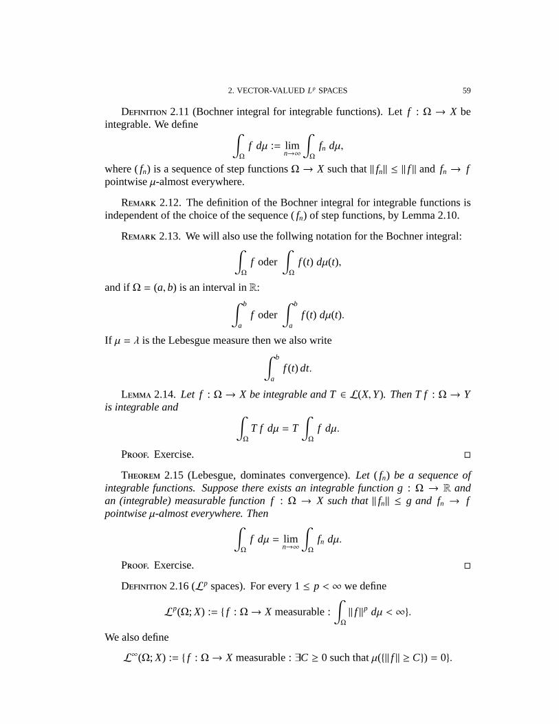
2. VECTOR-VALUED Lp SPACES 59

D 2.11 (Bochner integral for integrable functions). Letf : Ω → X beintegrable. We define ∫

Ω

f dµ := limn→∞

∫Ω

fn dµ,

where (fn) is a sequence of step functionsΩ → X such that‖ fn‖ ≤ ‖ f ‖ and fn → fpointwiseµ-almost everywhere.

R 2.12. The definition of the Bochner integral for integrable functions isindependent of the choice of the sequence (fn) of step functions, by Lemma 2.10.

R 2.13. We will also use the follwing notation for the Bochner integral:∫Ω

f oder∫Ω

f (t) dµ(t),

and ifΩ = (a,b) is an interval inR:∫ b

af oder

∫ b

af (t) dµ(t).

If µ = λ is the Lebesgue measure then we also write∫ b

af (t) dt.

L 2.14. Let f : Ω → X be integrable and T∈ L(X,Y). Then T f : Ω → Yis integrable and ∫

Ω

T f dµ = T∫Ω

f dµ.

P. Exercise.

T 2.15 (Lebesgue, dominates convergence).Let ( fn) be a sequence ofintegrable functions. Suppose there exists an integrable function g: Ω → R andan (integrable) measurable function f: Ω → X such that‖ fn‖ ≤ g and fn → fpointwiseµ-almost everywhere. Then∫

Ω

f dµ = limn→∞

∫Ω

fn dµ.

P. Exercise.

D 2.16 (Lp spaces). For every 1≤ p < ∞ we define

Lp(Ω; X) := f : Ω→ X measurable :∫Ω

‖ f ‖p dµ < ∞.

We also define

L∞(Ω; X) := f : Ω→ X measurable :∃C ≥ 0 such thatµ(‖ f ‖ ≥ C) = 0.

60 4. APPENDIX

L 2.17. For every1 ≤ p < ∞ we put

‖ f ‖p :=( ∫Ω

‖ f ‖p dµ)1/p.

We also put‖ f ‖∞ := inf C ≥ 0 : µ(‖ f ‖ ≥ C) = 0.

Then‖ · ‖p is a seminorm onLp(Ω; X) (1 ≤ p ≤ ∞).

R 2.18. A function‖ · ‖ : X → R+ on a real or complex vector space iscalled aseminormif

(i) x = 0⇒ ‖x‖ = 0,(ii) ‖λx‖ = |λ| ‖x‖ for everyλ ∈ K and allx ∈ X,

(iii) ‖x+ y‖ ≤ ‖x‖ + ‖y‖ for all x, y ∈ X.

D 2.19 (Lp spaces). For every 1≤ p ≤ ∞ we put

Np := f ∈ Lp(Ω; X) : ‖ f ‖p = 0

= f ∈ Lp(Ω; X) : f = 0µ-almost everywhere.

We define the quotient space

Lp(Ω; X) := Lp(Ω; X)/Np,

which is the space of all equivalence classes

[ f ] := f + Np, f ∈ Lp(Ω; X).

L 2.20. For every[ f ] ∈ Lp(Ω; X) ( f ∈ Lp(Ω; X)) the value

‖[ f ]‖p := ‖ f ‖p

is well defined, i.e. independent of the representant f . The function‖ · ‖p is a normon Lp(Ω; X). The space Lp(Ω; X) is a Banach space when equipped with this norm.

R 2.21. As in the scalar case we will in the following identifyfunctionsf ∈ Lp(Ω; X) with their equivalence classes[ f ] ∈ Lp(Ω; X), and we say thatLp isa function spacealthough we should be aware that it is only a space of equivalenceclasses of functions.

R 2.22. ForΩ = (a,b) an interval inR and forµ = λ the Lebesgue measurewe simply write

Lp(a,b; X) := Lp((a,b); X).We can do so since the spacesLp([a,b]; X) andLp((a,b); X) coincide since the endpointsa andb have Lebesgue measure zero and there is no danger of confusion.

L 2.23. LetΩ ⊂ Rn be open and bounded. Then C(Ω; X) ⊂ Lp(Ω; X) forevery1 ≤ p ≤ ∞.

P. Actually, for finite measure spaces, we have the more general inclusions

L∞(Ω; X) ⊂ Lp(Ω; X) ⊂ Lq(Ω; X) ⊂ L1(Ω; X)

if 1 ≤ q ≤ p ≤ ∞.

3. VECTOR-VALUED SOBOLEV SPACES 61

L 2.24. Let the measure space(Ω,A, µ) be such that Lp(Ω) is separablefor 1 ≤ p < ∞ (e.g.Ω ⊂ Rn be an open set with the Lebesgue measure). Let X beseparable. Then Lp(Ω; X) is separable for1 ≤ p < ∞.

P. By assumption the spacesLp(Ω) andX are separable. Let (hn) ⊂ Lp(Ω; X)and (xn) ⊂ X be two dense sequences. Then the set

F := f : Ω→ X : f = hn xm

is countable. It suffices to shows thatF ⊂ Lp(Ω; X) is total, i.e. spanF is dense inLp(Ω; X). This is an exercise.

T 2.25. LetΩ be as in lemma 2.24. Let1 < p < ∞ and assume that X isreflexive. Then the space Lp(Ω; X) is reflexive and

Lp(Ω; X)′ Lp′(Ω; X′).

P. Without proof.

3. Vector-valued Sobolev spaces

D 3.1 (Sobolev spaces). Let−∞ ≤ a < b ≤ ∞ and 1≤ p ≤ ∞. Wedefine

W1,p(a,b; X) := u ∈ Lp(a,b; X) : ∃v ∈ Lp(a,b; X)∀ϕ ∈ D(a,b)∫ b

auϕ′ = −

∫ b

avϕ.

Notation:v =: u′.

L 3.2. For every−∞ ≤ a < b ≤ ∞ and every1 ≤ p ≤ ∞ one hasW1,p(a,b; X) ⊂ Cb((a,b); X). For every u∈ W1,p(a,b; X) and every s, t∈ (a,b)one has

u(t) − u(s) =∫ t

su′(r) dr.

Bibliographie

1. H. Amann,Linear and Quasilinear Parabolic Problems: Abstract Linear Theory, Monographsin Mathematics, vol. 89, Birkhauser Verlag, Basel, 1995.

2. S. B. Angenent,Nonlinear analytic semiflows, Proc. Roy. Soc. Edinburgh115A (1990), 91–107.3. H. Brezis,Analyse fonctionnelle, Masson, Paris, 1992.4. R. Dautray and J.-L. Lions,Analyse mathematique et calcul numerique pour les sciences et les

techniques. Vol. I, INSTN: Collection Enseignement, Masson, Paris, 1985.5. , Analyse mathematique et calcul numerique pour les sciences et les techniques. Vol.

VIII , INSTN: Collection Enseignement, Masson, Paris, 1987.6. , Analyse mathematique et calcul numerique pour les sciences et les techniques. Vol. VI,

INSTN: Collection Enseignement, Masson, Paris, 1988.7. J. Escher, J. Pruss, and G. Simonett,A new approach to the regularity of solutions of parabolic

equations, Evolution Equations: Proceedings in Honor of J. A. Goldstein’s 60th Birthday, MarcelDekker, New York, 2003, pp. 167–190.

8. E. Feireisl and F. Simondon,Convergence for semilinear degenerate parabolic equations in sev-eral space dimensions, J. Dynam. Differential Equations12 (2000), 647–673.

9. D. Gilbarg and N. S. Trudinger,Elliptic Partial Differential Equations of Second Order, SpringerVerlag, Berlin, Heidelberg, New York, 2001.

10. A. Haraux,Systemes dynamiques dissipatifs et applications, Masson, Paris, 1990.11. E. Hille and R. S. Phillips,Functional Analysis and Semi-Groups, Amer. Math. Soc., Providence,

R.I., 1957.12. P. C. Kunstmann and L. Weis,Maximal Lp regularity for parabolic equations, Fourier multiplier

theorems and H∞ functional calculus, Levico Lectures, Proceedings of the Autumn School onEvolution Equations and Semigroups (M. Iannelli, R. Nagel, S. Piazzera eds.), vol. 69, SpringerVerlag, Heidelberg, Berlin, 2004, pp. 65–320.

13. J.-L. Lions,Quelques methodes de resolution des problemes aux limites non lineaires, Dunod,Gauthier-Villars, Paris, 1969.

14. E. M. Ouhabaz,Analysis of Heat Equations on Domains, London Mathematical Society Mono-graphs, vol. 30, Princeton University Press, Princeton, 2004.

15. H. Triebel,Theory of Function Spaces, Birkhauser, Basel, 1983.

63

Universite de Metz´ - IECL | Institut Élie Cartan de Lorrainechill/m2r0607.pdf · Universite de...

Documents

Transcript of Universite de Metz´ - IECL | Institut Élie Cartan de Lorrainechill/m2r0607.pdf · Universite de...