UNIVERSITA DEGLI STUDI DI PADOVA - unipd.ittesi.cab.unipd.it/52125/1/De__Min_Alessio_tesi.pdf ·...
149
UNIVERSITA’ DEGLI STUDI DI PADOVA DIPARTIMENTO DI INGEGNERIA INDUSTRIALE CORSO DI LAUREA MAGISTRALE IN INGEGNERIA ENERGETICA YEARLY ENERGY ANALYSIS OF CO2 REFRIGERATION SYSTEMS Relatore: prof. Davide Del Col Correlatore: prof. Brian Elmegaard res. Martin Ryhl Kærn eng. Kristian Fredslund Alessio De Min 1084145 ANNO ACCADEMICO 2015-2016
Transcript of UNIVERSITA DEGLI STUDI DI PADOVA - unipd.ittesi.cab.unipd.it/52125/1/De__Min_Alessio_tesi.pdf ·...

UNIVERSITA’ DEGLI STUDI DI PADOVA
DIPARTIMENTO DI INGEGNERIA INDUSTRIALE
CORSO DI LAUREA MAGISTRALE IN INGEGNERIA ENERGETICA
YEARLY ENERGY ANALYSIS OF CO 2 REFRIGERATION
SYSTEMS
Relatore: prof. Davide Del Col
Correlatore: prof. Brian Elmegaard
res. Martin Ryhl Kærn
eng. Kristian Fredslund
Alessio De Min
1084145
ANNO ACCADEMICO 2015-2016


To Mum and Dad


"There is a crank down in Apalachicola, Florida,
that thinks he can make ice by his machine
as good as God Almighty".
New York Globe, 1844.


AbstractThe present thesis was prepared at the Section of Thermal Energy, Department of Mechanical
Engineering, Technical University of Denmark (DTU), during the Erasmus exchange program.
During the last decades the refrigeration industry was involved in the increasing concern
about the environmental aspect. Synthetic refrigerant like CFCs and HCFCs have been banned
already from most of the industrialized countries because of the ozone depletion potential and
the greenhouse effect. Since 2008 the European Union has started to phase out also HFCs. The
necessity to replace these refrigerants has led research into other sustainable alternatives like
natural refrigerants. Among these, carbon dioxide seems to be the most promising solution.
The main disadvantage of CO2 is its low critical point. This means that when the environment
temperature is high the cycle has to work in transcritical operation, with higher losses and
consequently lower performances. The purpose of this project is to study different solutions
that can improve the COP of the system during the transcritical operation and see which one
performs better from the yearly analysis point of view. The solutions taken into consideration
are four: parallel compression, mechanical subcooling, cascade system and the use of an
ejector to recover expansion work. In the first part of the project these systems are studied
under fixed design conditions. In the second part the yearly analysis is performed using the
off-design model of the cycles for two different Italian cities: Milan and Naples. At the end
all the results are compared with a R404A cycle. The results show that the most promising
solution is the cycle using the ejector combined with the parallel compression. This system
is able to save 12.0% and 14.8% of energy during a year of operation in Milan and Naples
respectively. The normal parallel compression cycle achieves good performances too, saving
8.8% and 11.0% of energy in the two cities, the mechanical subcooling follows with 7.6% and
10.1%.
Keywords: Refrigeration systems; Natural refrigerant; Carbon dioxide; CO2; R744; Parallel
compression; Mechanical subcooling; Cascade system; Ejector; Yearly energy analysis.
v


Sommario
La seguente tesi è stata preparata al Dipartimento di Ingegneria Meccanica della Denmark
Technical University (DTU) grazie al programma di scambio Erasmus.
Durante gli ultimi decenni l’industria del freddo è stata scossa dal punto di vista normativo
a causa della scoperta del danno ambientale che i fluidi sintetici possono arrecare al nostro
pianeta se rilasciati in atmosfera. I refrigeranti come i CFC e gli HCFC sono già stati banditi dal
commercio in gran parte dei paesi industrializzati a causa del loro potenziale di distruzione
dell’ozono e dell’effetto serra. Dal 2008 l’Unione Europea ha emanato una serie di normative
in modo da iniziare ad escludere dal mercato anche gli HFC. La necessità di sostituire questi
refrigeranti sintetici ha condotto la ricerca a puntare il mirino su altre soluzioni più sostenibili
come i refrigeranti naturali. Questa categoria comprende diversi fluidi tra i quali l’acqua,
l’anidride carbonica, l’ammoniaca e gli idrocarburi. La CO2 tra tutti sembra essere il fluido più
promettente: è presente nell’atmosfera, è ininfiammabile, atossica, non provoca la distruzione
dello strato di ozono, il suo coefficiente di effetto serra è minimo ed ha elevati rendimenti
quando la temperatura esterna è inferiore a 25°C circa. Lo svantaggio principale della CO2 è la
bassa temperatura critica, il che significa che quando la temperatura esterna è alta il ciclo deve
lavorare in condizioni transcritiche, con maggiori perdite durante il processo di gas cooling
ed il processo di laminazione. L’obbiettivo di questo progetto è studiare diverse soluzioni
che siano in grado di aumentare il COP del sistema durante il funzionamento in condizioni
transcritiche e vedere quale tra queste è in grado di raggiungere il più alto grado di risparmio
energetico sotto il punto di vista di un analisi annuale. Le soluzioni prese in considerazione
sono quattro: la compressione parallela, con economizzatore e con sottoraffreddamento
integrato, il sottoraffreddamento meccanico, il sistema a cascata e l’uso di un eiettore per
recuperare il lavoro perso durante l’espansione, con e senza compressione parallela. I sistemi
studiati sono dunque sei più il ciclo base. Nella prima parte della tesi i cicli sono modellati e
studiati sotto condizioni di design fissate, in modo da poter ottimizzare i principali parametri
e fare un primo confronto tra i vari sistemi. Nella seconda parte le ottimizzazioni effettuate
sono utilizzate per scrivere i modelli in off-design con condizioni al contorno più specifiche.
Come già accennato, il principale problema dei cicli utilizzanti CO2 come fluido refrigerante
è il basso rendimento quando operano ad alte temperature. L’analisi energetica annuale è
dunque effettuata per due diverse città italiane: Milano, posta al nord e quindi con un clima
più freddo, e Napoli, che si trova al sud ed ha una temperatura media più elevata. Per calcolare
i risultati è stato utilizzato il Test Reference Year (TRY), l’analisi è dunque su base oraria (8760
valori). Riguardo il carico frigorifero è stato preso in considerazione un supermercato di taglia
vii

Abstract/Sommario
media con carico di picco pari a 100 kW.
I risultati mostrano che la soluzione migliore è il ciclo con eiettore combinato con la compres-
sione parallela che, comparato con il ciclo base, permette di risparmiare il 12,0% e il 14,8% di
energia nell’arco di un anno, a Milano e Napoli rispettivamente. La compressione parallela
semplice raggiunge anch’essa buoni risultati con un risparmio del 8,8% e del 11,0%, seguita dal
sottoraffreddamento meccanico con 7,6% e 10,1%. Il ciclo semplice con eiettore non raggiunge
buoni risultati a causa di alcune restrizioni che non permettono di utilizzare il dispositivo se
la temperatura è inferiore ai 25°C. Il sistema a cascata è sicuramente quello che raggiunge i
COP più elevati quando si opera ad alte temperature, perde tutto il suo vantaggio però quando
la temperatura esterna è inferiore ai 20°C. Siccome un impianto installato sia a Milano che
Napoli lavora per molte ore durante l’anno al di sotto di questo valore, il sistema a cascata non
è competitivo; lo potrebbe diventare nel caso in cui la temperatura di evaporazione vanga
abbassata.
Nell’ultimo capitolo della tesi è riportato il confronto tra i sistemi ad anidride carbonica stu-
diati e un ciclo base che utilizza R404A come fluido refrigerante. Viste le diverse caratteristiche
di scambio termico dei due fluidi, che portano gli scambiatori di calore a lavorare con ∆t
differenti è stata eseguita un’analisi di sensibilità variando, per il ciclo a R404A, la temperatura
di evaporazione e la differenza di temperatura tra aria e fluido al condensatore. I risultati
mostrano che anche nelle condizioni più sfavorevoli il ciclo con eiettore e compressione
parallela è in grado di utilizzare meno energia del ciclo a R404A durante il corso dell’anno. Le
due appendici della tesi, A e B, riportano rispettivamente i testi dei modelli compilati con EES
(Engineer Equation Solver) e due schemi per ogni sistema, uno che mostra il sistema mentre
opera in condizioni subcritiche e l’altro in condizioni transcritiche, riportandone i parametri
più importanti.
Parole chiave: Sistemi di refrigerazione; Refrigerante naturale; Anidride carbonica; CO2; R744;
Compressione parallela; Sottoraffreddamento meccanico; Sistema a cascata; Eiettore; Analisi
energetica annuale.
viii

Contents
Abstract v
Contents x
Nomenclature xi
1 Introduction 1
1.1 Background . . . . . . . . . . . . . . . . . . . . . . . . . . . . . . . . . . . . . . . . 1
1.2 History of CO2 . . . . . . . . . . . . . . . . . . . . . . . . . . . . . . . . . . . . . . . 3
1.3 Properties of CO2 . . . . . . . . . . . . . . . . . . . . . . . . . . . . . . . . . . . . . 4
1.4 CO2 as refrigerant . . . . . . . . . . . . . . . . . . . . . . . . . . . . . . . . . . . . . 9
2 Design conditions 11
2.1 Boundary conditions . . . . . . . . . . . . . . . . . . . . . . . . . . . . . . . . . . . 11
2.2 Base CO2 refrigeration cycle . . . . . . . . . . . . . . . . . . . . . . . . . . . . . . . 13
2.3 Parallel compressor economization . . . . . . . . . . . . . . . . . . . . . . . . . . 19
2.4 Parallel compressor economization with recooler . . . . . . . . . . . . . . . . . . 25
2.5 Refrigeration system with mechanical subcooling . . . . . . . . . . . . . . . . . . 31
2.6 Cascade system . . . . . . . . . . . . . . . . . . . . . . . . . . . . . . . . . . . . . . 39
2.7 Ejector expansion refrigeration cycle . . . . . . . . . . . . . . . . . . . . . . . . . 45
2.8 Ejector expansion refrigeration cycle with two suction groups . . . . . . . . . . . 57
3 Design conditions: comparison 63
4 Off-design conditions 69
4.1 Boundary conditions . . . . . . . . . . . . . . . . . . . . . . . . . . . . . . . . . . . 69
4.2 Base CO2 refrigeration cycle . . . . . . . . . . . . . . . . . . . . . . . . . . . . . . . 72
4.3 Parallel compressor economization . . . . . . . . . . . . . . . . . . . . . . . . . . 73
4.4 Parallel compressor economization with recooler . . . . . . . . . . . . . . . . . . 73
4.5 Refrigeration system with mechanical subcooling . . . . . . . . . . . . . . . . . . 74
4.6 Cascade system . . . . . . . . . . . . . . . . . . . . . . . . . . . . . . . . . . . . . . 74
4.7 Ejector expansion refrigeration cycle . . . . . . . . . . . . . . . . . . . . . . . . . 75
4.8 Ejector expansion refrigeration cycle with two suction groups . . . . . . . . . . . 76
4.9 Assumptions summary . . . . . . . . . . . . . . . . . . . . . . . . . . . . . . . . . . 79
ix
Contents
5 Off-design conditions: comparison 83
6 Yearly analysis 87
6.1 Real cooling load . . . . . . . . . . . . . . . . . . . . . . . . . . . . . . . . . . . . . 87
6.2 Climate conditions . . . . . . . . . . . . . . . . . . . . . . . . . . . . . . . . . . . . 88
6.3 Results . . . . . . . . . . . . . . . . . . . . . . . . . . . . . . . . . . . . . . . . . . . 90
7 Yearly analysis: comparison with an R404A cycle 93
7.1 R404A cycle . . . . . . . . . . . . . . . . . . . . . . . . . . . . . . . . . . . . . . . . 93
7.2 Results . . . . . . . . . . . . . . . . . . . . . . . . . . . . . . . . . . . . . . . . . . . 95
8 Conclusions 105
Bibliography 107
A Appendix A 111
A.1 Base cycle . . . . . . . . . . . . . . . . . . . . . . . . . . . . . . . . . . . . . . . . . 111
A.2 Parallel compression economization . . . . . . . . . . . . . . . . . . . . . . . . . 114
A.3 Parallel compression economization with recooler . . . . . . . . . . . . . . . . . 115
A.4 Refrigeration cycle with mechanical subcooling . . . . . . . . . . . . . . . . . . . 117
A.5 Cascade system . . . . . . . . . . . . . . . . . . . . . . . . . . . . . . . . . . . . . . 119
A.6 Ejector expansion refrigeration cycle . . . . . . . . . . . . . . . . . . . . . . . . . 121
A.7 Ejector expansion refrigeration cycle with two suction groups . . . . . . . . . . . 123
B Appendix B 127
x

Nomenclature
Abbreviations
2SG Two suction groupsBS Base cycleCFC ChlorofluorocarbonCO2 Carbon dioxideEERC Ejector expansion refrigeration cycleEES Engineering Equation SolverGWP Global Warming PotentialHCFC HydrochlorofluorocarbonHFC HydrofluorocarbonHFO HydrofluoroolefinIIR International Insitute of RefrigerationMS Mechanical subcoolingODP Ozone Depletion PotentialPCE Parallel compression economizationTEWI Total Equivalent Warming ImpactTRY Test Reference YearVCRC Vapour compression refrigeration cycle
xi

Nomenclature
Variables
COP coefficient of performance [-]cp specific heat at constant pressure [J/kgK]∆t temperature difference [°C]∆p pressure difference [bar]∆h specific enthalpy difference [J/kg]h specific enthalpy [J/kg]m mass flow rate [kg/s]η efficiency [-]p pressure [bar]P power [W]ϕ mass ratio(sec. compressor ej. cycle) [-]q specific heat [J/kg]r mass ratio [-]s specific entropy [J/kgK]t temperature [°C]w specific work [J/kg]x quality [-]y mass fraction [-]
xii
Nomenclature
Subscripts
0 cooling effectamb ambientav averagec compressorCO2 CO2 cyclecond condensationd, diff diffuserdis dischargeeco economizerej ejectorev evaporationgc gas coolerin inletis isentropiclift liftliq liquidm mass or motive nozzlemain main cyclemax maximummix mixing sectionopt optimalout outletr reals suction nozzlet theoreticalsec secondary cyclesub subcooling or subcooling cyclesc subcoolertot totalvar variation
xiii

1 Introduction
1.1 Background
During the last century the world energy consumption has been grown rapidly and is projected
to keep increasing in the next decades. Nowadays the amount of energy used by the entire
population is estimated around 12000 Mtep every year. Several studies have tried to figure out
if this growth have an asymptote, but all of them have different results. Indeed different factors
effect the energy consumption, like the population, the economy, the life behaviour and it is
particularly challenging understand how these factors will alter the results. Nevertheless the
world energy use is prospected to increase by 56% during the next 30 years [1], which is due,
like mentioned above, to the quickly population growth and the rising of developing countries.
Refrigeration industry is responsible for the 10-20% of the total consumption as estimate
from the International Institute of Refrigeration [2]. Moreover it has been discovered that
the chlorine substances used as refrigerant are very dangerous for the environment. For this
reason during the last decades the refrigeration sector was forced to face some radical changes.
CFCs (chlorofluorocarbons), invented in the 1930 by Thomas Midgley and then widely used
as refrigerants because of the high performance that they can achieve, were discovered to be
incredibly harmful for our planet in the middle of the 1980s. They are the main responsible for
the ozone depletion phenomena and they also have an high global warming potential (GWP).
GWP is an index that relates of a greenhouse gas to the CO2 emission over 100 years period (for
this reason CO2 has unitary GWP). CFCs were replaced by HCFCs (hydrochlorofluorocarbons).
Anyway this category still causes ozone depletion because of the atoms of chlorine inside the
molecules and still increases the green house effect when released in the atmosphere. CFCs
and HCFCs have been banned from all the industrialized countries that signed the Montreal
Protocol (1987) and the subsequent updates [3]. These refrigerants are almost off the market
nowadays and only their "brothers", the HFCs (hydrofluorocarbons), are trying to survive. Not
having chlorine atoms they are not dangerous for the ozone layer but they still have an high
GWP. The HFC refrigerants that were once excepted to be acceptable permanent replacement
fluids are now target of political actions due to their impact to the climate change. They are
included in the greenhouse gasses covered by the Kyoto Protocol(1997) and from 2008 the
1

Chapter 1. Introduction
European Union started to phase them out. The cold industry is now more than ever looking
for new sustainable solutions able to replace the old refrigerants once for all. The solutions
are two: using new chemical compounds, like HFOs (hydrofluoroolefins), with the risk that
they will be banned in few years too, or focus the effort in natural refrigerants. Thus there is an
increasing interest in technology based on the ecological natural refrigerants like air, water,
noble gases, ammonia, hydrocarbon and carbon dioxide. Among all of these, carbon dioxide
is the only non-flammable and non-toxic fluid that can operate in a vapour-compression
cycle below 0°C. In the last 3 decades, for the reasons reported above, carbon dioxide (CO2,
R744) has been rediscovered and the interest about it of the cold industry is keep growing. As
reported by Sharma et al., based on U.S. supermarkets, leakages of refrigerants are estimated
between 3% and 35% of the charge [4]. The wide range is due to the fact that new and old
equipment have very different performances. A leak of "traditional" refrigerant has a great
impact on the environment, for this reason the direct impact is becoming more important
every day. It is worth to remember that a refrigeration cycle has also an indirect impact. This
secondary effect take into account the emissions of greenhouse gases during the production
of the electricity needed by the cooling system in one year of operation. The TEWI index (Total
Equivalent Warming Impact) includes both these two effect and is used for the environmental
impact analysis of the refrigeration systems. Carbon dioxide has no ozone depletion potential
and unitary global warming potential, it is safe, cheap and available as secondary product
of many industrial processes. It also has very good properties for refrigeration applications.
However, CO2 has low critical temperature and its operating pressure is higher than traditional
refrigerants. This means that the cycle could work for many hours during a year as transcritical,
with more losses and consequently lower efficiency (see section 1.4). The purpose of this
project is to study some possible solutions able to increase the performances of the basic
1-stage vapour compression CO2 refrigeration cycle during a year of operation, focusing the
effort on improve the system especially when it is working in hot climates condition. The
improved system considered are four: parallel compression, mechanical subcooling, cascade
system and the use of an ejector to recover the expansion work. After a brief introduction
about history and proprieties of carbon dioxide as refrigerant, the above mentioned systems
will be modelled and studied. In the first part all the different cycles are presented under
fixed design conditions in order to understand their behaviour when applied in hot climate
conditions. Some assumptions will be made to simplified the analysis. The second part is
the main part of the project and it is about the yearly analysis of the systems. The design
conditions study of a certain cycle give important hints about its behaviour under specific
boundaries. Anyway a refrigeration system can face very different working conditions along
one year of operation. In order to follow these changing, off design models will be made with
more accurate assumptions. In the end a comparison with a R404A refrigeration cycle will
be presented. The models of each cycle have been made with the software EES (Engineering
Equation Solver)[5]. This software bases its CO2 calculations on the fundamental equation of
state provided by Span and Wagner [6]. The models used for the yearly analysis are proposed
in Appendix A. Appendix B shows how the most important variables of the studied cycles
change passing from a subcrtitical working condition to a supercritical one.
2

1.2. History of CO2
Figure 1.1 – Refrigerants progression [8].
1.2 History of CO2
Using as guideline the study of Pearson [7] a brief history of CO2 is here presented. Before that
fig.1.1, proposed by Calm [8], is reported in order to have a simply overview on the history of
the cold industry. It gives an interesting idea of the refrigerants used along the years, dividing
them in four generations.
Carbon dioxide has been discovered in the 18th century. During his experiment on magnesium
carbonate, the Scottish physician James Black came to the discovery of CO2. Anyway Black
was not interested in refrigeration. It seems that the first person proposing a closed cycle for
refrigeration has been Oliver Evans in 1805, but only 30 years later, in 1834, Evans’s friend
Jacob Persing was granted the British patent for his ethyl ether machine. Ethyl ether was the
first refrigeration fluid proposed because readily manufactured and already uses as solvent in
other application. After some trial with air and the discovery of the absorption refrigeration
cycle carbon dioxide finally make a breakthrough in 1866, thanks to the work of the American
Thaddeus Lowe that solve the problem of the compression of CO2 adapting an hydrogen
compressor used to fill military balloon for carbon dioxide. He was able to create ice using
a close loop but he never patented his idea. In those years other refrigerants were more
appreciated and the use of CO2 in refrigeration systems was delayed because of the problem
of the high working pressures. Carbon dioxide became a good option starting from 1887
3

Chapter 1. Introduction
when Raydt, Linde and Windhausen rediscovered it and started building the first cycles.
From 1887 onwards, CO2 gained favour as a refrigerant for marine applications due to the
safety that it ensures. Ammonia was still the leading refrigerant for stationary application.
From the beginning of the 20th century ammonia started to generate some safety concerns,
so the companies started to think different solutions to make the systems safer. One of
these solution was proposed by the Frick Company in 1932. They started installing cascade
systems with ammonia for the high temperature loop and CO2 for the low temperature loop.
Using a cascade system permitted also to avoid the CO2 cycle to work in transcritical mode.
Nevertheless carbon dioxide was not able to reverse the leadership of ammonia because of
its higher efficiencies. From the middle of the 20th century carbon dioxide was completely
abandoned due to the appearance of the CFCs in the market. In few years these synthetic
fluids removed all the other refrigerants from the cold industry. They had the efficiency
and flexibility of ammonia with the safety of carbon dioxide. Moreover in those years new
compressors running at higher speed were developed, making the systems smaller, cheaper
and easier to maintain. CO2 is having only now a real change to reach a leadership position
in the market. In fact from the end of the 20th century the cold industry had to face the
problem of the environmental impact of the synthetic refrigerants and had to look to new, or
old, environmental friendly solutions. The pioneer of the reappraisal of carbon dioxide was
Gustav Lorentzen ([9],[10]), that in 1990 published a patent application for a transcritical cycle
using CO2 for automotive application [11]. He started also organizing the IIR conferences
about new environmental friendly refrigerants. All the papers and the works presented at
these conferences pulled the carbon dioxide reborn as refrigerant.
1.3 Properties of CO2
Nowadays the proprieties of the carbon dioxide are well known and they are quite different
from the conventional refrigerants. In this section the most important features of CO2 are
presented and commented using as base the paper of Kim et al. [12]. Carbon dioxide is
colorless and odorless gas presents in the atmosphere with a concentration of about 0.04%
by volume. This natural chemical compound is composed by a carbon atom covalent double
bonded to two oxygen atoms. CO2 is then a natural refrigerant, non-flammable, non-toxic,
with no ozone depletion potential and negligible global warming potential. This features are
important because made it a very safe fluid. Fig.1.2 shows the phase diagram of CO2. Critical
temperature and pressure are respectively 31.1°C and 73.8 bar and the saturation pressure
at 0°C is 35 bar. These working pressures are much higher than those for the conventional
refrigerants. Above the critical temperature is not possible to transfer heat to the ambient
by condensation as in a traditional vapour compression cycle, but it has to be used a gas
cooler. In this case the heat transfer process occurs in the supercritical region where pressure
and temperature are not coupled and the pressure can be regulated independently in order
to optimize the working condition of the system. Fig.1.3 and fig.1.4 present the t-s and
the p-h diagram respectively. Fig.1.5 show the vapour pressure curve of CO2 compared
4

1.3. Properties of CO2
Figure 1.2 – Phase diagram of CO2 [12].
to other fluids. It is possible to see that the vapour pressure of CO2 is much higher than
the other refrigerants and so the steepness of the curve. This means that the temperature
change associated with a pressure drop in the evaporator is smaller compared with the other
fluids. Carbon dioxide presents also an higher volumetric refrigeration capacity compared
to the traditional refrigerants as shown in fig.1.6. This is due to the high vapour density, as
the volumetric refrigeration capacity is defined as the product between the latent heat of
evaporation and the vapour density. Fig.1.7 and fig.1.8 present the density of CO2 as function
of temperature and the ratio of liquid to vapour density for different fluids. From the first figure
is possible to observe that the density of CO2 changes quickly close to the critical point (this
behaviour could be observed also for the other proprieties [12]). The second one shows that
the density ratio of CO2 is smaller than the other refrigerants, this means a more homogeneous
two phase flow. This factor is important since it determines the flow pattern and consequently
the heat transfer coefficient [13]. Also the thermal conductivity of CO2 is better compared
to other refrigerants. Citing Kim et al. [12]: " In summary the thermodynamic and transport
properties of CO2 seem to be favourable in terms of heat transfer and pressure drop, compared
to other typical refrigerants".
5

Chapter 1. Introduction
Figure 1.3 – Temperature-entropy diagram of CO2.
Figure 1.4 – Pressure-enthalpy diagram of CO2.
6

1.3. Properties of CO2
Figure 1.5 – Vapour pressure for different refrigerants [12].
Figure 1.6 – Volumetric refrigeration capacity for different refrigerants [12].
7

Chapter 1. Introduction
Figure 1.7 – Density of CO2 as function of temperature for different pressure levels [12].
Figure 1.8 – Ratio of liquid to vapour density at saturation for different refrigerants [12].
8

1.4. CO2 as refrigerant
1.4 CO2 as refrigerant
The carbon dioxide 1-stage vapour compression cycle is nowadays well known in all his
features and components and it is widely used, mostly in northern Europe where the climate
conditions are favourable. The studies in the last years focused on how to improve the
performance of this system also when operating in hot climates. As seen in the previous
section the more remarkable property of CO2 compared to the conventional refrigerants is
the low critical temperature. For this reason the heat rejection will in most cases take place in
supercritical region. This cause an higher discharge pressure and it makes the cycle working
as transcritical. Transcritical operation means that the evaporation temperature is below
the critical point, while the heat rejection temperatures are over it. Some peculiarities of
transcritical cycles are here discussed.
1.4.1 Transcritical operation
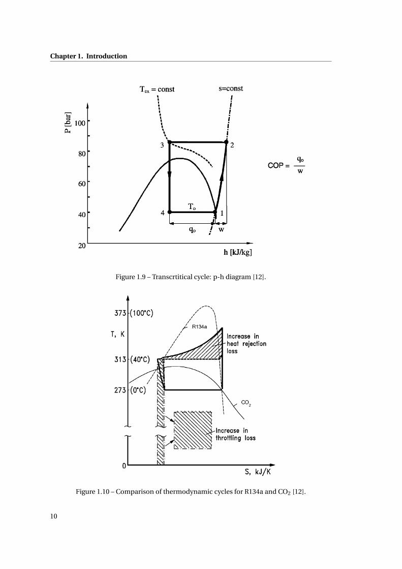
Fig.1.9 shows the p-h diagram of a CO2 transcritical cycle. During operation at high ambient
temperature the CO2 systems will work in transcritical conditions. In this case the heat
rejection at the high-side pressure will not take place in a condenser, but in a gas cooler
at supercritical pressure, therefore above the critical point where no saturation conditions
exist and temperature and pressure are independent. The main consequence of this is the
existence of an optimal gas cooler pressure. At fixed evaporative temperature, in conventional
systems the compressor work and consequently the COP depend on the discharge pressure:
higher the discharge pressure lower the performance. The behaviour is quite different in a
transcritical cycle. Looking at fig.1.9 is possible to see that varying the discharge pressure
has two different effects: increase the specific refrigerating capacity (q0) and increase the
the specific compressor work (w). The COP is defined as the ratio of q0 on w. Consequently,
increasing the discharge pressure, the COP reaches a maximum when the added capacity no
longer compensates for the additional work of compression. In the next chapters this optimal
pressure will be calculated for all the different systems, however due to the different operation
mode, the value will be different in each case. Regarding the losses, like reported by Kim et
al.: "the transcritical cycle suffers from a larger thermodynamic losses than an ’ordinary’ cycle
with condensation"[12]. This is due to the higher average temperature of heat rejection and
the larger throttling loss. The high average temperature is explained by the use of a gas-cooler
instead of a condenser. The throttling loss depends on the ratio cp,l i q /e. CO2 specific heat is
high and the evaporation enthalpy is low working near the critical point, then the throttling
loss become large. Fig.1.10 shows the additional thermodynamic losses of the CO2 cycle
compared with the R134a one, assuming equal minimum rejecting temperature and equal
evaporating temperature.
9
Chapter 1. Introduction
Figure 1.9 – Transcrtitical cycle: p-h diagram [12].
Figure 1.10 – Comparison of thermodynamic cycles for R134a and CO2 [12].
10

2 Design conditions
In this section different solutions are presented and then compared in order to understand
which one has the better performance during transcritical operation. As a reference for the
comparison the base CO2 cycle is used. The purpose is to improve the performance of this
system, especially when working with high ambient temperature. The four proposed solutions
are: parallel compression, mechanical subcooling, cascade system and the use of an ejector to
recover the expansion work. In the parallel compression two different designs will be studied,
the simple one with an economization and a second one with the subcooling integrated. For
the ejector cycle after using the normal one, a different solution with two suction groups
will be studied. Three different fluids will be used for the mechanical subcooling and for
the secondary loop of the cascade system, the fluids are: R404A, R134a and propane. After
the presentation of the boundary conditions needed for the modelling, all the cycles will be
presented with their features and some specific results will be discussed. In the next chapter
the overall results will be presented and the comparison of all of them will be made with
the same outdoor conditions. The models of each cycle have been made with the software
EES (Engineering Equation Solver, [5]) and are reported in Appendix A. The results presented
come from different simulations and have been collected in separate sheets where it has been
possible to postprocess them.
2.1 Boundary conditions
The different cycles are modelled in the same way in order to compare them. With this
aim some boundary conditions are required. These conditions are presented below, the
assumptions are made specifically for the design conditions modelling of the systems, with
the purpose of comparing different system for the same conditions. The entire systems have
been modelled based on mass and energy balance of every single component. The following
assumptions have been made for the analysis:
• Steady-state processes.
11
Chapter 2. Design conditions
• Isenthalpic expansion.
• Pressure drop and heat losses are neglected.
• Constant isentropic efficiency for the compressor is assumed to be 0.6 for all the cycles
and all the conditions.
• The processes in the heat exchangers are considered isobaric.
• The evaporation temperature is set to -2°C, however some simulations with different
value will be made in order to understand how this value effect the performance of the
cycle.
• The ambient temperature is set to 42.5°C. This choice has been made with the purpose
of simulating very hot ambient conditions; reason for this is to use the Italian climate
as the worst-case scenario. This temperature will be used to compare the cycle in
the next chapter, while in this one the behavior of the system will be studied also for
different conditions. In order to model the cycle for the off-design, it is necessary to
understand how to optimize the specific parameters of the systems also for different
ambient temperature.
• The gas cooler is assumed as air-cooled and the outlet temperature is set to be 5°C
higher than the ambient temperature.
• The fluid state at the outlet of the evaporator is considered saturated vapor.
• Superheat before the compressor is neglected.
• Separation and mixing process are isobaric.
• Fan power is neglected because it was assumed to be equal for all the systems.
• The cooling capacity is fixed to 100kW for all the cycles and all the operative conditions.
The choice is quite random and is useful only to compare the cycles with the same
value. For example Girotto et al. used for the same analysis a value of 120kW [14], while
Sawalha et al. used an higher value, i.e. 230kW [15]. In this first part of the project the
cooling capacity is supposed to be constant also if the ambient temperature is varying.
This is not a real assumption, because the lower the ambient temperature is the lower
the dispersion and consequently the cooling capacity. A more accurate load profile will
be used for the yearly analysis with the aim to model a system as close as possible to a
real one.
Other assumptions will be made in the next chapters when required specifically to each system.
Every section will be divided in three parts: the description of the system, the system analysis
and in the end the results preceded by a table that summarized the assumptions made for
every cycle.
12

2.2. Base CO2 refrigeration cycle
2.2 Base CO2 refrigeration cycle
In this chapter the base CO2 transcritical cycle will be presented and discussed. When using
the term base cycle the meaning is the 1-stage vapour-compression refrigeration cycle. This
cycle is the simpler cycle and it will be used as a reference to the comparison for all the other
systems. Before the presentation of the results and the comparison, all the different systems
will be presented in order to understand all the specific features.
2.2.1 Description of the system
The 1-stage vapour compression refrigeration cycle is made up from four main components,
where four different transformations happen. Fig.2.1 shows the layout of the system, the com-
ponents are respectively the compressor in the right, the gas cooler in the top, the throttling
valve in the left and the evaporator in the bottom. In all these components a different process
takes place. The evaporator make possible the heat exchange with the low temperature heat
sink, the ambient that have to be maintained at a certain temperature, and the gas cooler with
the high temperature heat sink, the external environment. Compressor and throttling valve
maintain an high pressure side and a low pressure side. The evaporator is a container or a
pipe system where the CO2 vaporizes at low pressure and temperature, this temperature has
to be below the temperature of the air in the refrigerated space. The latent heat necessary for
this aim is thus taken from this space. Fig.2.2 shows the logp-h diagram according with Fig.2.1.
It is possible to see at the outlet of the evaporator (state 1) that the fluid is saturated vapor,
usually the vapor will continue to absorb heat from the surrounding and become slightly
superheated before leaving the heat exchangers, but to make the model simpler the superheat
is considered nil. The fluid enters the compressor and reaches state 2 at the high-pressure
side, the compression is supposed to be non-isentropic. The high pressure is not a function
of the temperature like in the subcritical cycle therefore it will be possible to optimize it to
reach the best performance. From state 2 the fluid is cooled in the gas-cooler (state 2-3), from
there the fluid will expand in the throttling valve (state 3-4). The expansion process combined
with the high temperature heat exchange are the main source of losses in the transcritical
cycle. Moreover, working in transcritical mode means work at high pressures and then lower
compressor efficiency, so also the compression process could be improved. The purpose of the
modified cycles that will be presented is to reduce these losses. In the end, after the expansion
device, the fluid enters the evaporator (state 3).
For the base cycle the performance of the system are simply given as:
COP = (h1 −h4)
(h2 −h1)(2.1)
13

Chapter 2. Design conditions
GAS COOLER
EVAPORATOR4 1
23
Figure 2.1 – Layout of the base CO2 cycle.
Figure 2.2 – logp-h diagram of the base CO2 cycle.
14

2.2. Base CO2 refrigeration cycle
Figure 2.3 – COP vs gas-cooler pressure for different gas-cooler outlet temperatures (tev=-2°C).
2.2.2 System analysis
As mentioned in the beginning of this chapter all the cycle will be studied with the same
boundary conditions. Despite what the differences are in the systems, it is necessary to
understand how it is possible to achieve the best performance for each of them. Considering
the base cycle the only parameter that has to be optimized is the gas-cooler pressure. Before the
optimization, it is worth to see how the COP varies in function of this pressure. Fig.2.3 shows
the COP in function of the gas-cooler pressure for different gas-cooler outlet temperature. It
is possible to see that for every outlet temperature there is an optimal pressure in the way to
maximize the COP. This optimal pressure increase when the gas-cooler outlet temperature
increases, then when the ambient temperature increases.
Using the EES min/max function it has been possible to find the optimal pressure for the
different working conditions. Fig.2.4 shows the pressure as function of the gas-cooler outlet
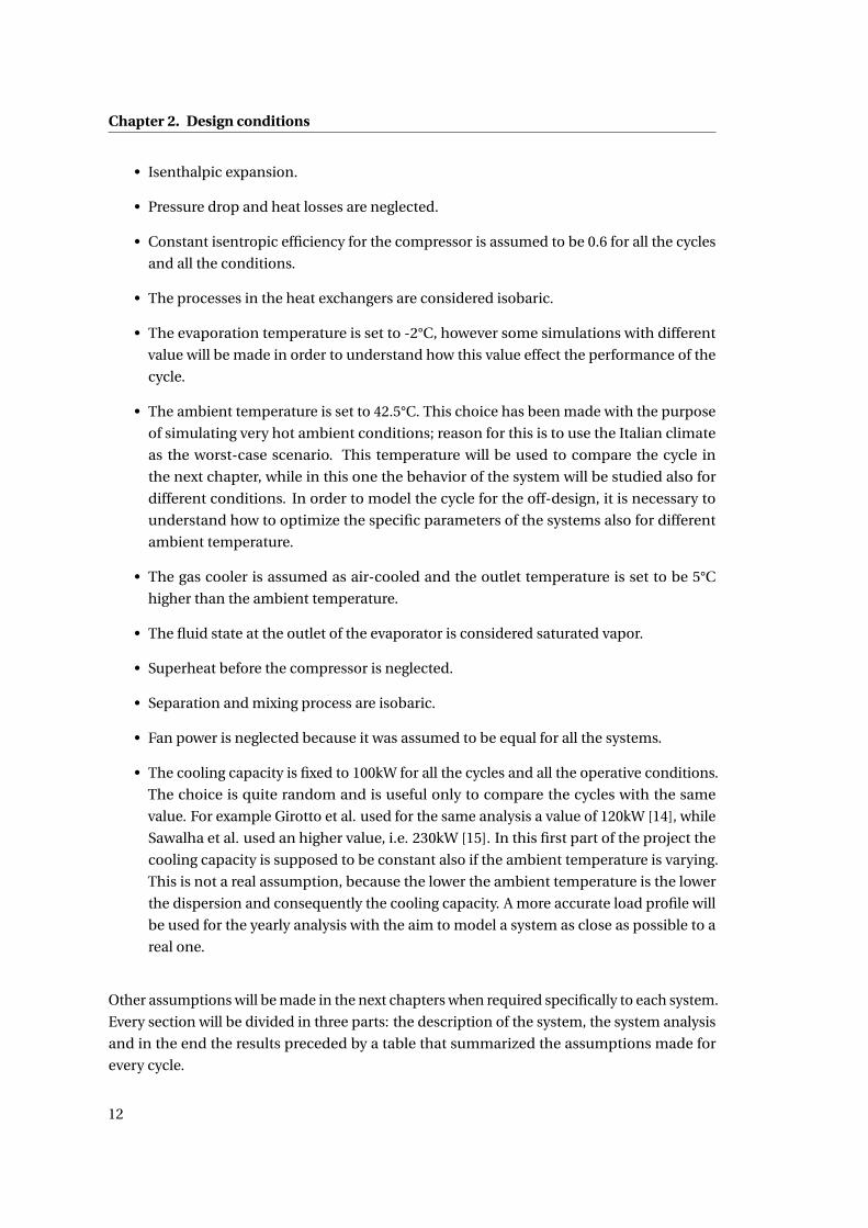
temperature, while the evaporative temperature is kept constant at -2°C. As expected the
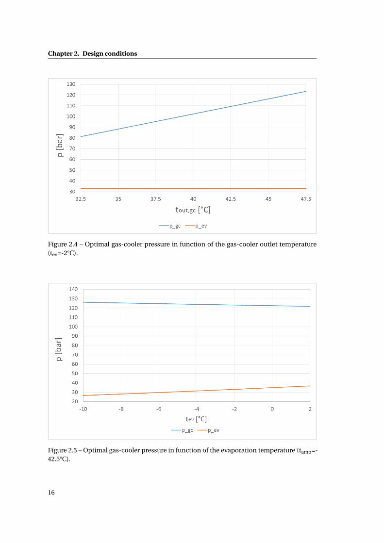
optimal pressure increase with the temperature. Fig.2.5 shows instead the pressure as function
of the evaporative temperature, while the ambient temperature is kept constant at 42.5°C, this
means that the gas-cooler outlet temperature is 47.5°C. In this case the lower the evaporative
temperature the higher the optimal gas-cooler pressure.
The results that have been obtained are compared with the correlation for the optimal heat
15
Chapter 2. Design conditions
Figure 2.4 – Optimal gas-cooler pressure in function of the gas-cooler outlet temperature(tev=-2°C).
Figure 2.5 – Optimal gas-cooler pressure in function of the evaporation temperature (tamb=-42.5°C).
16

2.2. Base CO2 refrigeration cycle
rejection pressure proposed by Liao et al. [16], another correlation is proposed by Ge et
al.[17]. The equation is expressed in terms of evaporation temperature and gas-cooler outlet
temperature and is here reported, the temperatures are in °C and the pressure is in bar.
pg c,opt = (2.778−0.0157 · tev ) · tg c,out + (0.381 · tev −9.34) (2.2)
The results found using this equation and the results obtained with the EES min/max function
are exactly the same.
17
Chapter 2. Design conditions
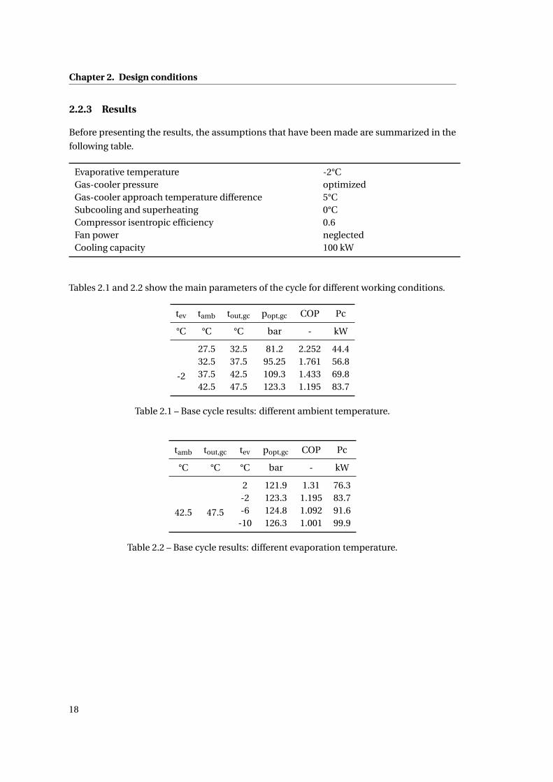
2.2.3 Results
Before presenting the results, the assumptions that have been made are summarized in the
following table.
Evaporative temperature -2°CGas-cooler pressure optimizedGas-cooler approach temperature difference 5°CSubcooling and superheating 0°CCompressor isentropic efficiency 0.6Fan power neglectedCooling capacity 100 kW
Tables 2.1 and 2.2 show the main parameters of the cycle for different working conditions.
tev tamb tout,gc popt,gc COP Pc
°C °C °C bar - kW
-2
27.5 32.5 81.2 2.252 44.432.5 37.5 95.25 1.761 56.837.5 42.5 109.3 1.433 69.842.5 47.5 123.3 1.195 83.7
Table 2.1 – Base cycle results: different ambient temperature.
tamb tout,gc tev popt,gc COP Pc
°C °C °C bar - kW
42.5 47.5
2 121.9 1.31 76.3-2 123.3 1.195 83.7-6 124.8 1.092 91.6
-10 126.3 1.001 99.9
Table 2.2 – Base cycle results: different evaporation temperature.
18

2.3. Parallel compressor economization
2.3 Parallel compressor economization
A large number of cycle modification are possible to improve the COP of vapour compression
refrigeration system. The main purpose of the modified cycle is to reduce the losses due
to the throttling process. Parallel compression economization system (PCE) is one of the
promising improvement techniques of vapour compression refrigeration cycle [18], where
refrigerant vapour is compressed to supercritical discharge pressure in two separate streams,
one coming from the evaporator and one coming from the separator or economizer. The main
difference from the base cycle is the introduction of the separator, which makes it possible for
the division of the throttling process into two stages. The effect of the separator is beneficial
for the system because it prevents the flash vapour to enter into the evaporator, this mean a
reduction of the compressor work and an increase of the refrigerant enthalpy difference in the
evaporator due to the less refrigerant quality at the inlet of it, but also the need of a secondary
compressor. In this section an optimization of the transcritical CO2 cycle with PCE is carried
out, it is important to know that in this case there are two parameters that can be optimized,
the gas-cooler pressure and the economizer or intermediate pressure.
2.3.1 Description of the system
The flow diagram and the corresponding p-h diagram are showed in Fig.2.6 and Fig.2.7 re-
spectively. After the gas-cooler (state 3) the fluid is expanded in the first expansion valve from
gas-cooler pressure to economizer pressure. The two-phase fluid (state 4) is then separated in
the economizer. The saturated liquid (state 5) is expanded again in the second expansion valve
from the intermediate pressure to the evaporator pressure (state 5-6) and then sent in the
evaporator to provide the cooling effect (state 6-1). The saturated vapour from the evaporator
and the separator are then compressed with two different compressors to the states 2 and 8
respectively. After the compression the two different flows are mixed (state 9) and sent in the
gas cooler where the rejection of the heat to the hot tank is achieved (state 9-3).
For unit total mass flow rate, the mass flow rate through the secondary compressor and the
main compressor are x4 and 1−x4 respectively, where x4 is a function of pressure and specific
enthalpy at state 4. The refrigerating effect of the evaporator is:
qev = (1−x4) · (h1 −h6) (2.3)
The specific work input to the compressors:
wc = (1−x4) · (h2 −h1)+x4 · (h8 −h7) (2.4)
In the end the performance of the system is given as:
COP = qev
wc(2.5)
19

Chapter 2. Design conditions
GAS COOLER
EVAPORATOR6 1
23
78
9
45
Figure 2.6 – Layout of the refrigeration cycle with parallel compression economization.
Figure 2.7 – logp-h diagram of the refrigeration cycle with parallel compression economization.
20

2.3. Parallel compressor economization
Figure 2.8 – COP vs economizer pressure for different gas-cooler outlet temperature (tev=-2°C).
2.3.2 System analysis
The operating condition of the system are the same as assumed for the base cycle according
with the boundary conditions listed in chapter 2.1. It is also important to remember that
separation and mixing processes are considered isobaric and adiabatic. As said in the previous
section the PCE cycle works between three level of pressure: the evaporative pressure, the
economizer pressure and the gas-cooler pressure. The first one is fixed by the evaporative
temperature, while the intermediate pressure is an influential parameter to find the best
performance along with the gas-cooler pressure. It is then necessary to optimize these two
pressures simultaneously [19].
Fig. 2.8 shows the COP in function of the economizer pressure for different gas-cooler outlet
temperature. It is possible to see that for each temperature there is a certain pressure where
COP attains the maximum value. The same result has been reached also by Sarkar and Agrawal:
"existence of the optimum economizer pressure is mainly on account of the changing slope of the
saturation curve"[19]. Increasing the economizer pressure means to increase the quality at the
inlet of the evaporator, then both the compressor work and the refrigeration effect decrease.
On the other hand they increase when the economizer pressure is lower. According to Sarkar
[18] it is possible to find the optimal condition when the compressor work is minimum and
the effect on the cooling capacity is negligible. Using the EES min/max function with two
degrees of freedom has been possible to find the optimal gas-cooler pressure and the optimal
21

Chapter 2. Design conditions
Figure 2.9 – Gas-cooler and economizer pressure vs gas-cooler outlet temperature (tev=-2°C).
Figure 2.10 – Gas-cooler and economizer pressure vs evaporative temperature (tamb=42.5°C).
22

2.3. Parallel compressor economization
economizer pressure in the same time for different working conditions. Fig.2.9 shows the
gas-cooler and the economizer pressure against the gas-cooler outlet temperature, the results
are also compared with the optimal gas-cooler pressure of the base cycle (yellow line). The
graph shows that the gas-cooler pressure for the base cycle is always higher in comparison to
the PCE cycle, this means that the parallel compressor economization is a useful technique
to increase the performance as well as decreasing the gas-cooler outlet pressure and the
discharge temperature. Fig.2.10 shows how the same pressures vary against the evaporative
temperature (ambient temperature set to 42.5°C). It is possible to see that the gas-cooler
pressure variation is almost nil, while the economizer pressure is decreasing going down with
the evaporative temperature.
23

Chapter 2. Design conditions
2.3.3 Results
Before presenting the results, the assumptions that have been made are summarized in the
following table.
Evaporative temperature -2°CGas-cooler pressure optimizedGas-cooler approach temperature difference 5°CEconomizer pressure optimizedSubcooling and superheating 0°CCompressor isentropic efficiency 0.6Fan power neglectedCooling capacity 100 kW
Tables 2.3 and 2.4 show the main parameters of the cycle for different working conditions.
tev tamb tout,gc popt,gc popt,eco COP Pc
°C °C °C bar bar - kW
-2
27.5 32.5 78.26 55.75 2.714 36.832.5 37.5 89.82 57.6 2.126 47.037.5 42.5 102.4 58.5 1.724 58.042.5 47.5 116.4 58.71 1.428 70.0
Table 2.3 – PCE results: different ambient temperature.
tamb tout,gc tev popt,gc popt,eco COP Pc
°C °C °C bar bar - kW
42.5 47.5
2 116.5 60.17 1.535 65.1-2 116.4 58.71 1.428 70.0-6 116.4 57.2 1.331 75.1
-10 116.4 55.67 1.242 80.5
Table 2.4 – PCE results: different evaporation temperature.
24

2.4. Parallel compressor economization with recooler
2.4 Parallel compressor economization with recooler
The performance of the base CO2 refrigeration system can be significantly improved by further
cooling the refrigerant after the gas-cooler. Parallel compressor economization cycle with
recooler, also called parallel compression cycle with integrated subcooling, is one of the
possibilities to achieve this goal. Thermodynamics of this cycle has been study for the first
time by Zubair in 1989 [20] and improved in the 1994 [21]. Later Khan et al. carried out an
overview on this system and studied the thermodynamic behaviour also under the second law
of the thermodynamic standpoint [22]. In all these studies it has been found that the system
performance improved when operating in situations when the gap between the gas-cooler
and the evaporating pressure is large, so in hot climate conditions. The major components of
the system are two compressors, two expansion valves, gas-cooler, evaporator, separator and
a recooler or subcooler. The components are almost the same of the PCE system, except for
the subcooler, from the literature it is possible to find this system as a modification of the one
seen in the last section [18].
2.4.1 Description of the system
Representation of the flow diagram and the corresponding p-h diagram are showed in Fig.2.11
and Fig.2.12 respectively. The exit transcritical vapour from the gas-cooler (state 3) is re-cooled
(state 3-8) by the secondary stream (state 4-5), which is at a lower temperature and pressure
due to the first expansion valve (state 3-4), which is located before the recooler. The flow
leaving the recooler is then expanded in the second throttling valve (state 8-9) before entering
the evaporator (state 9-1) where the cooling effect is performed. It is assumed that the exit
state of the cooling flow is saturated vapour (state 5) this state can be maintained by a proper
splitting of the refrigerant flow at the outlet of the gas-cooler. The saturated vapour from the
evaporator and the recooler are then compressed with two different compressors to states 2
and 6 respectively. They are then mixed (state 7) before entering the gas-cooler where the heat
is rejected to the ambient (state 7-3).
The model written with EES is based on the efficiency of the recooler, which is taken as 0.7,
given as:
ηsc = t3 − t8
t3 − t4(2.6)
Eq.2.7 and eq.2.8 are respectively energy conservation and the mass conservation for the
recooler:
msc · (h5 −h4) = mev · (h3 −h8) (2.7)
mtot = msc +mev (2.8)
25

Chapter 2. Design conditions
GAS COOLER
EVAPORATOR9 1
23
56
7
48
Figure 2.11 – Layout of the refrigeration cycle with parallel compression economization withrecooler.
Figure 2.12 – logp-h diagram of the refrigeration cycle with parallel compression economiza-tion with recooler.
26

2.4. Parallel compressor economization with recooler
Dividing the two mass flow rate for the unit total mass flow rate it’s possible to find the mass
fraction trough the subcooler and through the evaporator, given as:
ysc = msc
mtot(2.9)
yev = mev
mtot(2.10)
Then the performance of the system is given as:
COP = yev · (h1 −h9)
yev · (h2 −h1)+ ysc · (h6 −h5)(2.11)
2.4.2 System analysis
The layout of the parallel compressor economization system with integrated subcooling is
similar to the layout of the simple PCE, for this reason similar results are expected. Using
the same operating condition given in the chapter 2.1 it is possible to study this system and
then compare the result with PCE. The assumed ambient temperature forces the system to
transcritical operation, besides the system work between three level of pressure like the PCE
system, therefore as done for this cycle both the intermediate pressure and the gas-cooler
pressure have been optimized simultaneously.
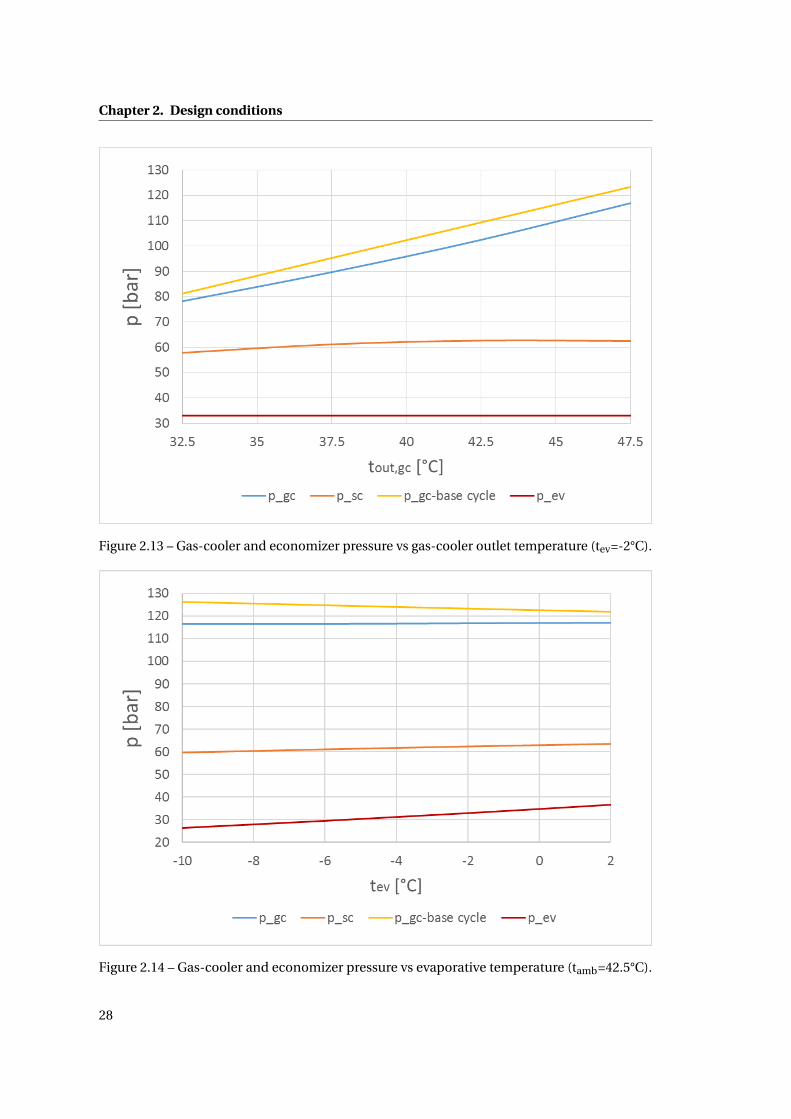
Fig.2.13 shows the gas-cooler and the economizer pressure against the gas-cooler outlet tem-
perature and fig.2.14 shows how the same pressures vary against the evaporative temperature
(ambient temperature is set to 42.5°C). The results are also compared with the optimal gas-
cooler pressure of the base cycle (yellow line). As expected the graphs are similar to the two
seen for the PCE and the same considerations are valid. In order to understand which one
of the two systems is better, the performance of the parallel compressor economization sys-
tem with integrated subcooling has been studied varying the subcooler efficiency and then
compared with the PCE system.
Fig.2.15 shows the COP against the efficiency of the subcooler (red line) for the PCE system with
recooler. As expected the COP increases if the efficiency increases. However the interesting
thing about the graph is the comparison with the PCE system. The orange line represents the
COP of the PCE system at the same condition, tamb=42.5°C and tev=-2°C, of the system with the
subcooler. The two lines cross at ηsc = 7.2, this mean that the PCE system with subcooling has
better performance than the normal one only if the efficiency of the recooler is higher than 7.2.
This fact could be explain thinking about the heat exchanger: the PCE system with subcooling
add a new component to the system, the recooler. This means a more complexity of the cycle
and a further heat exchange, therefore if the heat exchange has good performance, the COP is
better than the normal cycle, otherwise the losses in the heat exchange compromise also the
27
Chapter 2. Design conditions
Figure 2.13 – Gas-cooler and economizer pressure vs gas-cooler outlet temperature (tev=-2°C).
Figure 2.14 – Gas-cooler and economizer pressure vs evaporative temperature (tamb=42.5°C).
28

2.4. Parallel compressor economization with recooler
Figure 2.15 – COP vs ηsc , comparison with the PCE cycle.
performance of the entire system.
29

Chapter 2. Design conditions
2.4.3 Results
Before presenting the results, the assumptions that have been made are summarized in the
following table.
Evaporative temperature -2°CGas-cooler pressure optimizedGas-cooler approach temperature difference 5°CRecooler pressure optimizedRecooler efficiency 0.7Subcooling and superheating 0°CCompressor isentropic efficiency 0.6Fan power neglectedCooling capacity 100 kW
Tables 2.5 and 2.6 show the main parameters of the cycle for different working conditions.
tev tamb tout,gc popt,gc popt,sub COP Pc
°C °C °C bar bar - kW
-2
27.5 32.5 78.18 57.83 2.679 37.332.5 37.5 89.67 61.15 2.11 47.437.5 42.5 102.4 62.64 1.717 58.242.5 47.5 116.9 62.48 1.422 70.3
Table 2.5 – PCE with subcooling results: different ambient temperature.
tamb tout,gc tev popt,gc popt,sub COP Pc
°C °C °C bar bar - kW
42.5 47.5
2 117.1 63.6 1.534 65.2-2 116.9 62.48 1.422 70.3-6 116.7 61.2 1.32 75.8
-10 116.7 59.77 1.227 81.5
Table 2.6 – PCE with subcooling results: different evaporation temperature.
30

2.5. Refrigeration system with mechanical subcooling
2.5 Refrigeration system with mechanical subcooling
As said in the previous section the performance of the base CO2 refrigeration system can be
significantly improved by further cooling the refrigerant after the gas-cooler. The subcooling
allows the refrigerant to enter the evaporator with low quality, thus increasing the specific
cooling capacity of the plant and for the transcritical systems also reducing the optimal
heat rejection pressure. However these improvement come with a price, as reported by
Thorton et al.:"The amount of subcooling provided to the main cycle must equal the heat
addition to the subcooling cycle evaporator. The heat addition to the subcooling cycle must be
rejected in the subcooling cycle condenser/gas cooler at the cost of the work of the subcooling
cycle compressor"[23]. The mechanical subcooling, that can be called dedicated mechanical
subcooling, is only one of the possible subcooling technologies (in the previous section 2.4
the integrated mechanical subcooling has been studied) and the literature is full of promising
results. The mechanical subcooling was investigated under the first thermodynamic law
standpoint by Thornton et al. in 1994 [23], a more precise analysis has been carried out later
by Khan [24]. The system is made by two different cycles: the main one, with CO2, where the
cooling effect is achieved and the secondary one, necessary to subcool the carbon dioxide after
the gas cooler. The components of the first one are the same as for the base CO2 refrigeration
system with the addition of the subcooler, which is also the evaporator of the secondary cycle.
In this study three different refrigerants have been used to run the subcooling cycle: R404A,
R134a and propane.
2.5.1 Description of the system
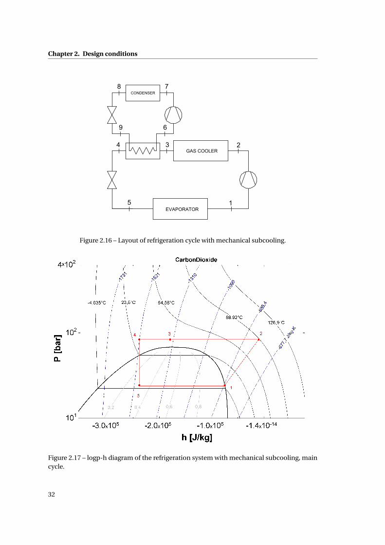
The layout of the system and the corresponding p-h diagram for the CO2 main cycle are
showed in Fig.2.16 and Fig.2.17 respectively. The main cycle is a 1-stage transcritical vapor
cycle with the addition of the subcooler after the gas-cooler, where the refrigerant is further
cooled (state 4-5) rejecting the heat to the secondary flow. The secondary fluid absorbs the
heat from the CO2 while evaporating (state 9-6). Both cycles perform the heat rejection, in the
condenser of the subcooling cycle and in the gas-cooler of the primary cycle, to the same hot
sink, the ambient temperature.
In order to write the model with EES it is necessary to add some specific boundary condi-
tions. Regarding the primary cycle, as done for the other cycles, to obtain the gas-cooler
outlet temperature (state 3) an approach of 5°C temperature difference from the ambient
temperature has been chosen. The subcooler outlet temperature (state 4) is obtained consid-
ering a determinate temperature difference in the heat exchanger (∆tsub). For the secondary
cycle have been considered only fluids working in subcritical conditions. The condensing
pressure is chosen considering a temperature difference from the environment of 8°C. The
conditions of the refrigerant at the outlet of the condenser and the evaporator are respectively
saturated liquid and saturated vapor. The isentropic efficiency of the compressor is assumed
to be 0.6 and constant (more precise condition will be taken into consideration in the second
31
Chapter 2. Design conditions
GAS COOLER
EVAPORATOR5 1
2349 6
78CONDENSER
Figure 2.16 – Layout of refrigeration cycle with mechanical subcooling.
Figure 2.17 – logp-h diagram of the refrigeration system with mechanical subcooling, maincycle.
32
2.5. Refrigeration system with mechanical subcooling
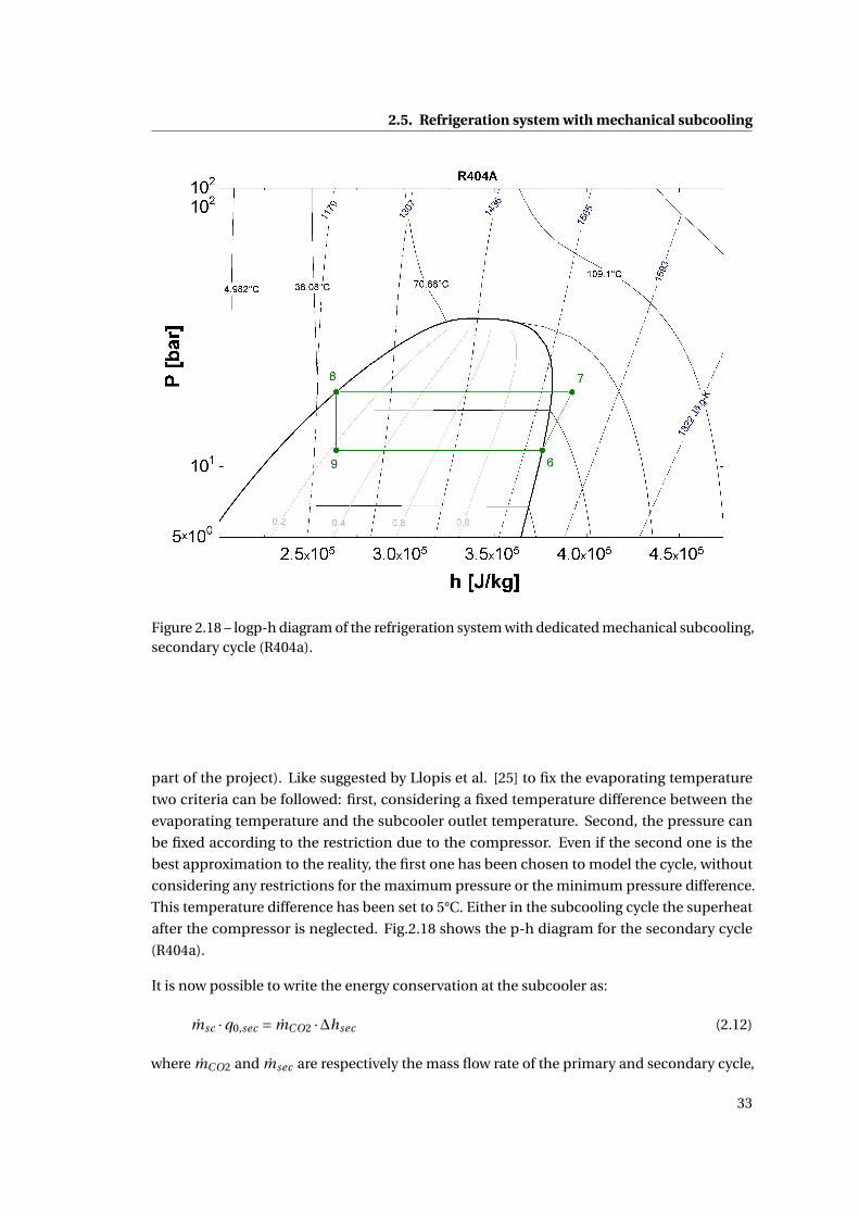
Figure 2.18 – logp-h diagram of the refrigeration system with dedicated mechanical subcooling,secondary cycle (R404a).
part of the project). Like suggested by Llopis et al. [25] to fix the evaporating temperature
two criteria can be followed: first, considering a fixed temperature difference between the
evaporating temperature and the subcooler outlet temperature. Second, the pressure can
be fixed according to the restriction due to the compressor. Even if the second one is the
best approximation to the reality, the first one has been chosen to model the cycle, without
considering any restrictions for the maximum pressure or the minimum pressure difference.
This temperature difference has been set to 5°C. Either in the subcooling cycle the superheat
after the compressor is neglected. Fig.2.18 shows the p-h diagram for the secondary cycle
(R404a).
It is now possible to write the energy conservation at the subcooler as:
msc ·q0,sec = mCO2 ·∆hsec (2.12)
where mCO2 and msec are respectively the mass flow rate of the primary and secondary cycle,
33

Chapter 2. Design conditions
q0,sec = h6 −h9 and ∆hsub = h3 −h4. The performance of the cycle is given by:
COP = mCO2 ·q0
mCO2 ·wc,CO2 +msec ·wc,sec(2.13)
where q0,wc,CO2 and wc,sec are respectively the specific cooling capacity, the specific work of
the primary compressor and the specific work of the secondary compressor. Using the energy
conservation at the subcooler [2.12] the overall COP can be expressed as:
COP = q0
wc,CO2 + ∆hsubCOPsec
(2.14)
Where the performance coefficient of the secondary cycle is:
COPsec =q0,sec
wc,sec(2.15)
Regarding the subcooling degree it needs to be mentioned that although any value is theo-
retically possible, there is a practical limit that has to be considered. Mentioning Llopis et al
[25]: "for centralized systems, the maximum subcooling degree would be equal to the approach
temperature between gas-cooler outlet and the environment (in this case 5°C), since higher
subcooling degrees will be lost due to heat transfer to the environment during the distribution
of the refrigerant. For stand-alone systems this subcooling degree can be increased a bit". The
system will still be studied without any restriction, but in the next chapter the results will be
presented considering a reasonable degree of subcooling.
Usually the components of the secondary cycle or subcooling cycle are smaller than those of
the main cycle. In order to know how small the secondary cycle is compared to the main one
in terms of mass flow and power consumption, two new parameters, the mass ratio and the
power ratio, are introduced and defined respectively as:
rm = msec
mCO2(2.16)
rp = Pc,sec
Pc,CO2= rm · wc,sec
wc,CO2(2.17)
2.5.2 System analysis
As explain above, the system has been modelled using a determinate temperature difference
between the evaporating temperature of the secondary cycle and the outlet subcooler temper-
ature (CO2 side). In the first part of this section the consequences of varying the temperature
difference will be studied. Since the results are similar for all the three secondary fluids only the
graphs for the propane will be presented. In next chapter the overall results for all of them will
34

2.5. Refrigeration system with mechanical subcooling
Figure 2.19 – Gas-cooler pressure vs gas-cooler outlet temperature (tev=-2°C).
be shown. Fig.2.20 show the COP against the ∆tsub for different gas-cooler outlet temperature.
It can be seen that the best performance is achieved at a certain grade of subcooling, which
varies with the temperature at the outlet of the gas-cooler, the higher the ambient temperature
is, the higher the temperature difference needed to reach the maximum COP. Fig.2.21 presents
how the optimized gas-cooler pressure (the one that permits to have the best performance)
varies with the ∆tsub . The lines have an U shape, therefore as expected at the begin, the higher
the subcooling grade is, the lower the optimal pressure, but after a certain point the pressure
starts to increase because of the shape of the isotherms. It is interesting to see that the lower
pressure for each gas-cooler outlet temperature does not match with the higher COP condition
as seen in the previous graph. The graphs show also that the value of subcooling that achieve
the best performance, is always higher than the practical limit.
As done for the other systems fig.2.19 shows the difference between the optimal gas-cooler
pressure of the base cycle and the gas-cooler pressure of the cycle with dedicated mechanical
subcooling (propane, ∆tsub=10°C), the difference increases when the ambient temperature
increases.
35

Chapter 2. Design conditions
Figure 2.20 – COP vs ∆tsub for different gas-cooler outlet temperature (tev=-2°C, propane).
Figure 2.21 – Optimized gas-cooler pressure vs ∆tsub for different gas-cooler outlet tempera-ture (tev=-2°C, propane).
36

2.5. Refrigeration system with mechanical subcooling
2.5.3 Results
Before presenting the results, the assumptions that have been made are summarized in the
following table.
Main cycleEvaporative temperature -2°CGas-cooler pressure optimizedGas-cooler approach temperature difference 5°C∆tsub 5°C, 10°C and 15°CSuperheating 0°C
Secondary cycleCondenser temperature difference 8°CEvaporator approach temperature difference 5°CSubcooling and superheating 0°C
Compressor isentropic efficiency 0.6Fan power neglectedCooling capacity 100 kW
Tables 2.7, 2.8 and 2.9 show the main parameters of the cycle using for secondary fluid propane,
R404A and R4134a respectively. It has been chosen to report the results with different value of
∆tsub and different ambient temperature to see how these parameters effect the performance
together. It can be seen that the highest performance is reached by the R134a, followed by
propane and then R404A.
tev tamb ∆tsub popt,gc ym yp COPsub COP Pc
°C °C °C bar - - - - kW
-2 32.5
5 87.55 0.1275 0.05349 10.53 2.084 48.010 87.25 0.2063 0.1183 7.603 2.249 44.515 87.85 0.258 0.1874 5.851 2.312 43.3
-2 42.5
5 112.8 0.08958 0.02667 10.56 1.394 71.710 104.9 0.2116 0.09225 7.618 1.573 63.615 102.5 0.3105 0.1769 5.858 1.683 59.4
Table 2.7 – MS results: propane.
37

Chapter 2. Design conditions
tev tamb ∆tsub popt,gc ym yp COPsub COP Pc
°C °C °C bar - - - - kW
-2 32.5
5 87.77 0.3157 0.05691 9.622 2.075 48.210 87.55 0.51 0.1259 6.943 2.227 44.915 88.2 0.6401 0.2005 5.328 2.277 43.9
-2 42.5
5 113.1 0.24 0.02976 9.353 1.39 71.910 105.8 0.5484 0.09955 6.733 1.556 64.315 104.4 0.7807 0.1849 5.156 1.65 60.6
Table 2.8 – MS results: R404A.
tev tamb ∆tsub popt,gc ym yp COPsub COP Pc
°C °C °C bar - - - - kW
-2 32.5
5 87.49 0.2409 0.05265 10.77 2.087 47.910 87.18 0.3897 0.1165 7.777 2.254 44.415 87.77 0.4866 0.1843 5.983 2.32 43.1
-2 42.5
5 112.7 0.1678 0.02596 10.88 1.395 71.710 104.6 0.3992 0.09058 7.847 1.577 63.415 102 0.5901 0.1756 6.032 1.69 59.2
Table 2.9 – MS results: R134a.
38

2.6. Cascade system
2.6 Cascade system
The cascade system is a refrigeration system working with two different cycles and two different
fluids. Like for the system with dedicated mechanical subcooling, the cascade system cannot
be properly considered a CO2 system because of the presence of a different fluid. However the
purpose of this study is to understand how to use CO2 to achieve the best performance in hot
climate condition. The best quality of the cascade system is that it makes possible to avoid
working in transcritical conditions. This is because the CO2 is used in the low temperature
cycle while another fluid, with higher critical point, is used for the high temperature cycle
or secondary cycle. Cascade systems using CO2 have been widely studied in the past years
combined with different fluids, synthetic or natural, as R134a [26], R404A [27] or propane
[28]. The common result for all these studies is that a cascade system achieves really good
performance when the temperature difference between the hot sink and the cold sink is large.
EVAPORATOR4 1
239 6
78CONDENSER
Figure 2.22 – Layout of the refrigeration cascade system.
2.6.1 Description of the system
The flow diagram of the cascade system is shown in Fig.2.6. The system is made by two
different 1-stage vapor cycle, the condenser of the low temperature cycle (that work with CO2)
rejects the heat (state 2-3) to the evaporator of the high temperature cycle (state 9-6). The
cooling effect is achieved in the low temperature evaporator (state 4-1) while the heat rejection
to the environment happens in the high temperature condenser (state 7-8). In order to model
the system some new specific boundary conditions have to be specified. The conditions of the
refrigerant at the outlet of the condenser and the evaporator, are respectively saturated liquid
39

Chapter 2. Design conditions
(a) CO2 (b) R404A
Figure 2.23 – logp-h diagrams of the cascade refrigeration system.
and saturated vapor for both the cycles, superheat is neglected. The isentropic efficiency of
both the compressors is assumed to be 0.6 and constant. No restrictions have been taken into
consideration concerning the minimum pressure difference. The condensing pressure of the
high temperature cycle is chosen considering a temperature different from the environment
of 8°C. While the condensing pressure of the low temperature cycle is optimized using the EES
min-max function in order to reach the best performance. At the end a constant temperature
difference of 5°C is used to find the evaporative temperature of the high-pressure cycle.
Following the same procedure used for the dedicated mechanical subcooling [2.5], i.e. us-
ing the energy conservation in the common heat exchanger, makes it possible to write the
performance of the cycle as:
COP = q0
wc,CO2 + qcond ,CO2
COPsec
(2.18)
Where the performance coefficient of the high temperature cycle is:
COPsec =q0,sec
wc,sec(2.19)
2.6.2 System analysis
As stated earlier three different fluids have been used as refrigeration fluid in the high-pressure
cycle. The choice has been made to understand which one can achieve the best performance.
The results have can be seen in fig.2.24. The graph shows that R134a achieves the best COP,
followed by propane and then R404A.
Fig.2.25 shows the COP of the secondary cycle and the optimized CO2 condensing temperature
versus the ambient temperature. The first graph is similar to fig.2.24, this mean that the overall
COP is mainly influenced by the performance of the high pressure cycle. The second one shows
40

2.6. Cascade system
Figure 2.24 – COP vs ambient temperature (tev=-2°C).
Figure 2.25 – COP of the high pressure cycle and optimized CO2 condensing temperature vsambient temperature (tev=-2°C).
Figure 2.26 – rm and rp vs ambient temperature (tev=-2°C).
41

Chapter 2. Design conditions
the difference between the three fluids concerning the optimal condensing temperature.
In order to understand which amount of power has been used by the two cycles fig.2.26 has
been proposed. The graphs show the mass flow ratio and the power ratio in function of the
ambient temperature. These two parameter are defined respectively as:
rm = msec
mCO2(2.20)
rp = Pc,sec
Pc,CO2= rm · wc,sec
wc,CO2(2.21)
The figure shows that at tamb=42.5°C the amount of power needed by the high pressure cycle
is more than three times the power needed by the low pressure cycle for all the refrigerants.
2.6.3 Results
Before presenting the results, the assumptions that have been made are summarized in the
following table.
Main cycleEvaporative temperature -2°CCondenser pressure optimized
Secondary cycleCondenser temperature difference 8°CEvaporator approach temperature difference 5°C
Subcooling and superheating 0°CCompressor isentropic efficiency 0.6Fan power neglectedCooling capacity 100 kW
Tables 2.10, 2.11 and 2.11 show the main parameters of the cycle used for secondary fluid
propane, R404A and R4134a respectively. The results are reported for the different ambient
temperature and the same evaporation temperature (-2°C). It can be seen that as found out
for the mechanical subcooling in the previous section, the highest performance is reached by
the R134a, followed by propane, then R404A.
42

2.6. Cascade system
tev tamb pcond,CO2,opt tcond,CO2,opt rm rp COPsub COP Pc
°C °C bar °C - - - - kW
-2
27.5 46.97 11.71 0.794 2.253 4.522 2.824 35.432.5 47.3 12 0.8349 2.63 3.789 2.469 40.537.5 47.5 12.32 0.8815 3.022 3.221 2.171 46.142.5 48.06 12.65 0.935 3.433 2.765 1.915 52.2
Table 2.10 – Cascade system results: propane.
tev tamb pcond,CO2,opt tcond,CO2,opt rm rp COPsub COP Pc
°C °C bar °C - - - - kW
-2
27.5 47.82 12.45 1.957 2.255 4.272 2.653 37.732.5 48.3 12.86 2.101 2.649 3.529 2.288 43.737.5 48.84 13.32 2.273 3.073 2.944 1.976 50.642.5 49.45 13.82 2.487 3.544 2.465 1.702 58.8
Table 2.11 – Cascade system results: R404A.
tev tamb pcond,CO2,opt tcond,CO2,opt rm rp COPsub COP Pc
°C °C bar °C - - - - kW
-2
27.5 46.88 11.64 1.493 2.232 4.593 2.862 34.932.5 47.2 11.92 1.567 2.6 3.858 2.508 39.937.5 47.55 12.22 1.651 2.981 3.289 2.212 45.242.5 47.92 12.54 1.746 3.378 2.833 1.958 51.1
Table 2.12 – Cascade system results: R134a.
43

2.7. Ejector expansion refrigeration cycle
2.7 Ejector expansion refrigeration cycle
An important field of research for improving the performance of refrigerating systems is
the reduction of the losses through the expansion valve. Since the critical temperature of
carbon dioxide is usually lower than the heat rejection temperature, the cycle has to work in
transcritical conditions. Compared with refrigerating cycle of conventional refrigerants the
CO2 transcritical cycle has a larger pressure difference between the gas-cooler pressure and
the evaporating pressure, this means that also the losses through the throttling valve are larger.
In order to recover the expansion losses and increase the cycle efficiency, it has been proposed
to replace the throttling valve with a different device. There are three kinds of devices that can
be used with this purpose:
• Expansion turbine[29]: it is probably the best way to recover the expansion work, but
there are some issues that interfere with the development of this device. First of all there
is the problem with the cost, especially for small size application, the expansion from
transcritical region to the two-phase region is still not theoretically clear and low quality
two-phase flow make the device prone to damage.
• Vortex tube[30]: the vortex tube is a device without moving part. Inside it the gas is
expanding from the gas-cooler pressure to the evaporation pressure and then divided
into three fractions: saturated liquid, saturated vapor, and superheated gas. Some
studies regarding it seem promising, but they are at early stage, not enough experimental
data is available and the mechanism inside the tube is still not clear.
• Ejector: in literature there can be found a great amount of researches about the device,
from the first law standpoint[31] and also from the second law standpoint [32][33]. The
results are promising and different companies started to use it in trial plants. Therefore
also real data is available[34]. Comparing with the expansion turbine the cost is reduced
and the lifetime increased (there is no moving part in this case). Thus the use of an
ejector in the CO2 transcritical cycle seems to be the most promising solution.
In the ejector expansion refrigeration cycle (EERC) an ejector is used instead of the throttling
valve to recover the kinetic energy of the expansion process. Using the ejector the compressor
suction pressure is higher than it would be normally, this means less compression work and
higher performance. Generally the compressor efficiency increases if the pressure ratio is
lower. Another beneficial effect is achieved in the evaporator: using an ejector instead of an
expansion valve the cycle is provided also with a liquid-vapor separator, which results in the
cooling capacity of the cycle to be increased. In this section the EERC will be studied following
the model proposed by Kornhauser[35]. The first part is focused just on the ejector with the
purpose of understand how it works and what is the best way to model it, followed by the
second part where the ejector model will be insert in the system and the whole cycle will be
studied.
45

Chapter 2. Design conditions
Figure 2.27 – Schematic of constant area ejector flow model[33].
2.7.1 Ejector principle and design
The working principle of the ejector is based on converting the energy otherwise lost in the
throttling process into kinetic energy and then again in pressure energy through a diffuser.
The ejector can be divided into four different parts: a primary nozzle, a suction chamber, a
mixing chamber and a diffuser. Two different flows are entering the ejector: the primary flow
and the secondary flow. The primary flow, or nozzle flow, is at high pressure (then coming
from the gas-cooler) and the secondary flow, or suction flow, is at low pressure (coming from
the evaporator). The basic principle is to use the expansion work of the high-pressure flow
to achieve a total flow at the outlet section of the ejector with a pressure higher than the
secondary flow. The primary flow expands in the motive nozzle and exits with high velocity
and low pressure, usually the velocity is supersonic. The low pressure creates an entrainment
effect for the secondary flow that is then entrained in the suction chamber also thanks to high
velocity of the primary flow. The two flows are then mixed in the mixing chamber and the
momentum is transferred from the primary to the secondary flow. The mixture has a certain
velocity that is recovered in order to increase the pressure in the diffuser. Fig.2.27 shows the
different parts of the ejector.
The ejector can be described by several dimensionless parameters. The first one is the mass
entrainment ratio [2.22] which is defined as the ratio of the secondary mass flow over the
primary mass flow, and shows the ability of the ejector sucking the flow from the evaporator.
The second one is the pressure lift [2.23] defined as the difference between the diffuser outlet
pressure and the suction inlet pressure. In the end the ejector efficiency [2.24], defined to
quantify the efficiency of the expansion work recovery. Elbel et al.[36] define the efficiency as
the ratio of the compression work obtained over the maximum potential expansion work. The
first term is the work recovered by the secondary flow between the suction inlet pressure and
46

2.7. Ejector expansion refrigeration cycle
the diffuser outlet pressure. The second one is the ideal expansion work between the nozzle
inlet pressure and the diffuser outlet pressure.
r = ms
mm(2.22)
pl i f t = pdi f f ,out −ps,i n (2.23)
ηe j =ms · (h(pdi f f ,out ; ss,i n)−hs,i n)
mm · (hm,i n −h(pdi f f ,out ; sm,i n))(2.24)
2.7.2 Ejector model
In this section the equations used to describe the behavior of the flow in the ejector are
presented. Mass, momentum and energy conservation are used to find the outlet conditions
of each section supposing that the conditions at the inlet are known. From literature there
can be found different kinds of ejector model, the majority refers to two ideal cases: the
constant pressure mixing model and the constant area mixing model. However none of these
represents properly what happens through the ejector, but are still a sufficient tool when
studying the EERC. More complicated models can be used, but their application is limited
and the results are always questioned. In this project the model used is the constant pressure
model proposed by Kornhauser[35], an "homogeneous equilibrium model" for the two phase
flow. The analysis assumes that: the flow in the ejector is a one-dimensional homogeneous
equilibrium flow, properties and velocities are constant over cross sections. Thus the analysis
is one-dimensional, the refrigerant is at all time in thermodynamic quasi-equilibrium, the
processes in the motive nozzle, in the suction nozzle and in the diffuser could be expressed in
terms of efficiencies. These efficiencies take into account the losses caused by that the process
is not reversible and an eventual shock effect. Mixing section process efficiency is supposed
unitary, kinetic energy is negligible outside the ejector. About the efficiencies Liu et al. [37]
made an important review investigating the literature, finding out that values of 0.7-0.9 are
assumed for every part of the ejector. In another study [38] they also proposed three empirical
correlations to calculate the efficiencies. Since the purpose of this study is not to study the
ejector model, but study the performance of a cycle using an ejector, the efficiencies of the
motive nozzle, the suction nozzle and the diffuser have been chosen as constant among the
most used in literature and are respectively: ηm = ηs = 0.8 and ηd = 0.75. Another important
assumption that has been made to be able to write the model is that the flows in the motive
nozzle and in the suction nozzle at the entrance of the mixing chamber are assumed to have
the same pressure. In the constant pressure model this pressure is also the pressure in the
47

Chapter 2. Design conditions
mixing chamber and has to be lower than the evaporative pressure, then: pm,out =ps,out =pmi x .
The value to choose for this parameter will be discussed in the next section. The equations
used are now presented.
If the inlet conditions are known and the value for the pressure at the outlet of the primary
nozzle is assumed, the isentropic enthalpy at the outlet can be found.
hm,out ,i s = h(sm,i n ; pm,out ) (2.25)
By using the definition of the motive nozzle’s isentropic efficiency the enthalpy at the nozzle
outlet is defined.
ηm = hm,out −hm,i n
hm,out ,i s −hm,i n(2.26)
Then, the energy conservation is used the outlet velocity assuming that the kinetic energy at
the inlet of the nozzle is negligible.
hm,i n = hm,out +w2
m,out
2(2.27)
Similarly to what has been written for the primary nozzle the equations governing the sec-
ondary nozzle are presented.
hs,out ,i s = h(ss,i n ; ps,out ) (2.28)
ηs =hs,out −hs,i n
hs,out ,i s −hs,i n(2.29)
hs,i n = hs,out +w2
s,out
2(2.30)
As said above ps,out and pn,out are given and equal. In the mixing section the mass conserva-
tion can be written as:
mtot = mm +ms (2.31)
Using the definition of entrainment ratio[2.22] the momentum conservation and the energy
conservation at the exit of the mixing chamber are respectively:
wmi x,out = 1
1+ r·wm,out + r
1+ r·ws,out (2.32)
48

2.7. Ejector expansion refrigeration cycle
hmi x,out = 1
1+ r· (hm,out + r ·hs,out )−
w2mi x,out
2(2.33)
The enthalpy of the stream at the diffuser exit can be found by applying the principle of energy
conservation through the ejector.
hd ,out =hm,i n + r ·hs,i n
1+ r(2.34)
By using the definition of the motive nozzle’s isentropic efficiency the enthalpy at the nozzle
outlet is defined.
ηd = hd ,out ,i s −hmi x,out
hd ,out −hmi x,out(2.35)
Then, the pressure at the outlet of the ejector is found using the isentropic enthalpy.
pd ,out = p(smi x,out ;hd ,out ,i s) (2.36)
The quality of the fluid at the exit of the ejector is found by using the diffuser pressure pd ,out
and the enthalpy hd ,out . However to ensure the cycle continuity the quality of the stream
leaving the ejector should be approved with the follow equation.
xd ,out =1
1+ r(2.37)
The equations reported do not allow an accurate investigation of pressure and velocity gra-
dients inside the ejector. The purpose of this project is not to study the inside phenomena
of the ejector, but the performance of the entire system. Cross-sectional homogeneity and
thermodynamic equilibrium are incorrect assumption.
2.7.3 Description of the system
Now that the ejector has been introduced the overall system can be described. The flow
diagram and the corresponding p-h diagram are showed in Fig.2.28 and Fig.2.29 respectively.
The high-pressure fluid coming from the gas-cooler (state 1) enters the motive nozzle and
expands (state 2). The secondary flow from the evaporator (state 3) enters the suction nozzle
and expands (state 4) until the same pressure gets mixed in the mixing chamber with the
primary flow at a constant pressure (p2 = p4 = p5). The mixed flow enters the diffuser and here
its velocity drops until it almost reaches a stagnation state while the pressure increases(state 6).
The mixture leaving the ejector enters the separator and separates itself into saturated liquid
and saturated vapor. The saturated vapor (state 7) enters the compressor where it has been
compressed until the gas-cooler pressure (state 8). After this it enters the gas-cooler where the
heat rejection into the environment takes place (state 8-1). The saturated liquid (state 9) then
49

Chapter 2. Design conditions
leaves the separator and enters the throttling valve where it reaches the evaporative pressure
(state 10). In the evaporator the cooling effect is performed (state 10-3) and the fluid enters
the ejector again.
The equations for the cycle performance are written below. The cooling capacity per unit
mixture flow mass is:
q0 = r
1+ r· (h3 −h10) (2.38)
The compressor power consumption per unit mixture flow mass is:
wc = 1
1+ r· (h8 −h7) (2.39)
The performance of the system can be written as:
COP = q0
wc(2.40)
2.7.4 System analysis
As it has been said above, to solve the model it is necessary to make an assumption regarding
the pressure at the outlet of the nozzles and in the mixing chamber (p2 = p4 = p5). In literature
this value is always chosen considering a certain pressure different between the evaporative
pressures. The value used in almost all the studies is p3 −p4 = 0.3bar . Before using the same
value some simulations have been made in order to understand if there is an optimum value
for this pressure and how the performance of the cycle varies.
Fig.2.30 and fig.2.31 shows how the COP of the system and the ejector efficiency vary against
the pressure difference for different gas-cooler outlet temperatures. It can be seen that the lines
concerning the COP are almost constant for each temperature, this means that the value of
the pressure difference it not that important when the entire cycle is taken into consideration.
However if we are looking at the ejector performance, the second figure shows that the ejector
efficiency has a maximum value that is different for each gas-cooler outlet temperature.
Considering that the COP is almost constant, it has been decided to follow the literature and
use p3 −p4 = 0.3bar for modeling the cycle with the purpose to avoid more complications in
the ejector model. The optimization of the system was performed determining the gas-cooler
pressure that gives the maximum system COP for the given condition. The COP based analysis
represent only a first-law investigation. A second law investigation can be made on exergy
base to reflect the behavior for each of the single components. Fangtian et al. [32] show in
their paper that the exergy losses with an ejector cycle can be reduced by the 25% compared
with the base cycle. An important consideration has also been made regarding the minimum
value of the pl i f t . After discussing with Kristian Fredslund[39] from Danfoss, it became clear
that the minimum value of this parameter has to be at least 4 bar. This is because of the
proper operation of the throttling valve that cannot work if the pressure difference is lower
50
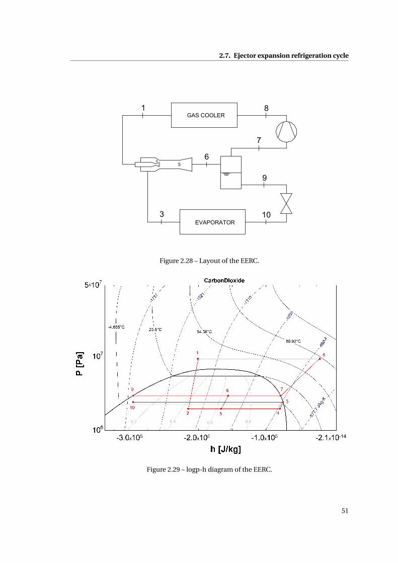
2.7. Ejector expansion refrigeration cycle
GAS COOLER
EVAPORATOR3 10
81
67
9524
Figure 2.28 – Layout of the EERC.
Figure 2.29 – logp-h diagram of the EERC.
51

Chapter 2. Design conditions
Figure 2.30 – COP vs (p3 −p4) (tev=-2°C).
Figure 2.31 – ηe j vs (p3 −p4) (tev=-2°C).
52

2.7. Ejector expansion refrigeration cycle
Figure 2.32 – Operation map of the ejectors based on experimental data, numbers representthe ejector efficiency[34].
than this value. It can be seen in the p-h diagram [2.31] that the pressure different through
the expansion valve (p9 −p10) is the same pressure different defined as pl i f t = (p6 −p3) in
the equation 2.23. Thus, to maintain 4 bar of pressure different, the ejector has to be able to
ensure the same lift. Regarding the design conditions with transcritical operation this is not
a problem since the gas-cooler pressure is high enough to let the ejector maintain an high
pressure lift. The problem starts when the ambient temperature is lower than 25°C, the ejector
is not able to ensure 4 bar of pressure lift and therefore has to be by-passed. This problem
concerns the off-design condition of the model, it will be further discussed in chapter 4. To
conclude this section a comparison of the theoretical ejector efficiency with a real one has
been made in order to understand if the ejector model is close to the reality. The experimental
data proposed by Kriezi and Fredslund [34] in fig.2.32 has been used (in the y axis dp means
pl i f t ).
With these values it has been possible to make an interpolation in order to write the ejector
efficiency in function of the pl i f t . Fig.2.33 shows the results. The orange line is the theoretical
ejector efficiency calculates with the equation 2.24, the blue line represent instead the real
ejector efficiency calculated using the experimental data. The graph shows that for the values
of pl i f t from 7 bar to 10 bar the two lines are close, meaning that the model is following the
real data, for values lower than 7 bar the lines gradually splits up.
53

Chapter 2. Design conditions
Figure 2.33 – Ejector efficiency vs pressure lift, comparison with the real data.
54

2.7. Ejector expansion refrigeration cycle
2.7.5 Results
Before presenting the results, the assumptions that have been made are summarized in the
following table.
Evaporative temperature -2°CGas-cooler pressure optimizedGas-cooler approach temperature difference 5°CEjector model constant pressure modelOutlet nozzles pressure 0.3 bar less than evaporative pressureMotive nozzle efficiency 0.8Suction nozzle efficiency 0.8Diffuser efficiency 0.75Subcooling and superheating 0°CCompressor isentropic efficiency 0.6Fan power neglectedCooling capacity 100 kW
Tables 2.13 and 2.14 shows the main parameters of the cycle for different working conditions.
It is important to repeat that the mixing pressure has been fixed at 0.3 bar lower than the
evaporation pressure. The choice to fix it and not to optimized it has been made for the reason
that the performance are barely affected by this value [2.30].
tev tamb popt,gc pdis,ej plift ηe j ,r ηe j ,t COP Pc
°C °C bar bar bar - - - kW
-2
27.5 81.2 38.01 4.97 0.2338 0.3006 2.719 36.7832.5 95.25 39.39 6.35 0.2555 0.2927 2.157 46.3637.5 109.3 40.94 7.90 0.2935 0.2853 1.783 56.0942.5 123.3 42.69 9.65 0.267 0.2784 1.511 66.18
Table 2.13 – EERC results: different ambient temperature.
tamb tev popt,gc pdis,ej plift ηe j ,r ηe j ,t COP Pc
°C °C bar bar bar - - - kW
42.5
2 121.9 46.53 9.79 0.2513 0.2779 1.647 60.72-2 123.3 42.69 9.65 0.267 0.2784 1.511 66.18-6 124.8 39.1 9.47 0.2829 0.2786 1.389 71.99
-10 126.3 35.75 9.26 0.2976 0.2786 1.281 78.06
Table 2.14 – EERC results: different evaporation temperature.
55


2.8. Ejector expansion refrigeration cycle with two suction groups
2.8 Ejector expansion refrigeration cycle with two suction groups
In this section the ejector expansion refrigeration cycle will be modified in order to make it
possible for a certain fraction of the secondary flow to skip the ejector after the evaporator.
This modification has been suggested by Kristian Fredslund [39], with the aim to model a
cycle as closer as possible to how a real refrigeration system is made. The basic idea is to use
two compressors instead of one so the flow at the exit of the compressor can go through the
ejector or can be directly compressed from the evaporative pressure to the gas-cooler pressure.
The main purpose of this modification is to make it possible for a reduction of the suction
flow when the primary flow is not able to ensure a minimum pressure lift of 4 bar. The real
advantage of this cycle compared with the normal one is shown in the second part of the
project. However in this part the cycle and the new equations that describe it will be presented.
The ejector model is the same as described in section 2.7.
2.8.1 Description of the system
The flow diagram and the corresponding p-h diagram are showed in Fig.2.34 and Fig.2.35.
The system is similar to the one seen in the last section. The flow coming from the gas-cooler
(state 1) enters the motive nozzle and expands (state 2) until the same pressure of the mixing
section (p2 = p4 = p5). This pressure is considered constant and 0.3 bar below the evaporative
pressure for the reasons explained previously [2.7]. The flow at the outlet from the evaporator
(state 11) is divided into two different flows, the first one; the suction flow (state 3) expands
in the suction nozzle until the mixing pressure and is then mixed with the primary flow. The
second one (state 12) skips the ejector and is compressed until the gas-cooler pressure (state
13) by the secondary compressor. The mixed flow in (state 5) enters the diffuser in the ejector
and its velocity decrease until almost a stagnation state while the pressure increase and the
pressure lift is achieved (state 6). After this the fluid enters the separator where the vapour
part (state 7) is compressed until the gas-cooler pressure by the main compressor (state 8) and
then mixed with the flow coming from the secondary compressor. The flow (state 14) enters
into the gas-cooler for then to reject the heat into the environment (state 14-1). Going back to
the separator, the liquid part (state 9) is expanded in the throttling valve until the evaporative
pressure and is then sent into the evaporator to achieve the cooling effect (state 10-11).
It has not been possible to find literature on a model like the one proposed here, all the
equations that have been used to describe it have been found and checked by the author.
In order to explain the equations describing the system it is necessary to introduce a new
parameter, which tell how much of the evaporative flow skips the ejector. The factor is
dimensionless and defined as the ratio of the mass flow skipping the ejector on the mass flow
through the evaporator.
ϕ= m12
m11(2.41)
57

Chapter 2. Design conditions
GAS COOLER
EVAPORATOR11 10
141
67
9524
138
312
Figure 2.34 – Layout of the EERC with two suction groups.
Figure 2.35 – logp-h diagram of the EERC with two suction groups.
58

2.8. Ejector expansion refrigeration cycle with two suction groups
The equations used to model the ejector are the same as in the previous section except for the
last one, the equation describing the quality of the fluid at the exit of the ejector that ensure
the cycle continuity [2.37]. With another flow in the cycle all the mass conservations have to
be modified in order to take into consideration also the factor ϕ. The follow equation can be
written.
xd ,out = x6 = 1− r
(1+ r ) · (1−ϕ)(2.42)
Using the definition of ϕ[2.41] and r[2.22], it is now possible to write all the equations describ-
ing the system performance per unit of mixture flow mass (the flow mass leaving the ejector)
as followed. The cooling capacity per unit mixture flow mass is:
q0 = r
(1+ r ) · (1−ϕ)· (h3 −h10) (2.43)
The main compressor power consumption per unit mixture flow mass is:
wc,mai n =(1− r
(1+ r ) · (1−ϕ)
)· (h8 −h7) (2.44)
The secondary compressor power consumption per unit mixture flow mass is:
wc,sec = r ·ϕ(1+ r ) · (1−ϕ)
· (h13 −h12) (2.45)
The heat rejected at the gas-cooler per unit mixture flow mass is:
q0 = 1
1+ r· (h14 −h1) (2.46)
And in the end the performance of the system can be written as:
COP = q0
wc,mai n +wc,sec(2.47)
2.8.2 System analysis
As explained in the previous section the second compressor added to the system makes it
possible to skip the ejector, and here the consequences of this modification will be studied.
The higher the ϕ is the lower the mass flow rate going through the ejector is. Fig.2.36 shows
how the pressure lift varies against ϕ for different gas-cooler outlet temperature. It is possible
to see that with higher values of ϕ the ejector ensures higher pressure lift. This is exactly the
purpose of having two compressor, this modification will be made possible to be able to use
the ejector also with low ambient temperature as will be shown in the chapter regarding the
off-design conditions of the system.
59

Chapter 2. Design conditions
Figure 2.36 – Pressure lift vs ϕ.
60

2.8. Ejector expansion refrigeration cycle with two suction groups
2.8.3 Results
Before presenting the results, the assumptions that have been made are summarized in the
following table.
Evaporative temperature -2°CGas-cooler pressure optimizedGas-cooler approach temperature difference 5°CEjector model constant pressure modelOutlet nozzles pressure 0.3 bar less than evaporative pressureMotive nozzle efficiency 0.8Suction nozzle efficiency 0.8Diffuser efficiency 0.75ϕ optimizedSubcooling and superheating 0°CCompressor isentropic efficiency 0.6Fan power neglectedCooling capacity 100 kW
Tables 2.15 and 2.16 show the main parameters of the cycle for different working conditions.
From the tables it is possible to see that the performances are similar to the ejector cycle with
only one compressor. The real advantage of the modified cycle will be shown in the chapter
regarding the yearly analysis.
tev tamb popt,gc ϕopt pdis,ej plift ηe j ,t COP Pc
°C °C bar - bar bar - - kW
-2
27.5 81.2 0.6704 43.44 10.40 0.2586 2.773 36.0632.5 95.25 0.6309 45.41 12.37 0.2561 2.197 45.5237.5 109.3 0.5803 47.22 14.18 0.2542 1.813 55.1642.5 123.3 0.5121 48.77 15.73 0.2533 1.532 65.27
Table 2.15 – EERC with two suction groups results: different ambient temperature.
61

Chapter 2. Design conditions
tev tamb popt,gc ϕopt pdis,ej plift ηe j ,t COP Pc
°C °C bar - bar bar - - kW
42.5
2 121.9 0.4489 45.23 12.19 0.2598 1.664 60.10-2 123.3 0.5121 48.77 15.73 0.2533 1.532 65.27-6 124.8 0.5617 49.47 16.43 0.2463 1.413 70.77
-10 126.3 0.6019 49.99 16.95 0.2391 1.306 76.57
Table 2.16 – EERC with two suction groups results: different evaporation temperature.
62
3 Design conditions: comparison
To conclude the first part of the project, the comparison of the results concerning the design
condition operation are here presented. All the results come from computational simulation
with the support of the software EES. All the cycles seen in chapter 2 are compared with
the 1-stage CO2 vapour compressor reference cycle under different points of view. All the
observations presented in this chapter refer to the chosen operating conditions of the systems.
Since the project is about a supermarket installation in Italy, as explained in the previous
chapter the design ambient temperature has been chosen for simulate the worst case scenario,
a really hot climate conditions with an ambient temperature of 42.5°C. The evaporation
temperature and the cooling capacity are -2°C and 100kW respectively and concerning the
dedicated mechanical subcooling a value of ∆tsub=10° has been chosen. Fig.3.1 shows the
optimal gas-cooler pressure for all the cycles, excluding the cascade system since in this case
the working condition are subcritical. The mechanical subcooling system is the one that
permits the cycle to work with the lowest pressure ratio among the others (-14.9% for propane,
-14.2% for R404A and -15.2% for R134a using the base cycle value as comparison), but also the
PCE and the PCE with subcooling achieve a useful drop of the gas-cooler pressure, -5.6% and
-5.2%. The optimization of the pressure for the ejector cycles gives the same results as the base
cycle. Fig.3.2compares the performance for all the systems. At this high ambient temperature
the cascade system, no matter which secondary fluid is used, reaches the best performance
with a COP of 1.958 if R134a is used. In this case the COP increment is 63.7%, 60.3% for
propane and 42.4% for R404a. The increase for the MS cycles is around 30%, 19.5% for the
PCE and 28.2% for the ejector cycle with two suction groups. In the end Fig.3.3 compares the
power consumption. The result are similar to the COP results, the largest power consumption
drop is achieved by the cascade systems, -39% for the R134a, followed from MS cycles, ejector
cycles and then the PCE cycle. Tab.3.1 summarizes the values discussed above.
63

Chapter 3. Design conditions: comparison
Figure 3.1 – Optimal gas-cooler pressure: comparison.
64

Figure 3.2 – COP: comparison.
65

Chapter 3. Design conditions: comparison
Figure 3.3 – Power consumption: comparison.
66

popt,gc COP Pc popt,gc,var COPvar Pc,var
bar - kW % % %
Base cycle 123.3 1.195 83.68 0.0% 0.0% 0.0%PCE 116.4 1.428 70.03 -5.6% 19.5% -16.3%PCE sub 116.9 1.422 70.32 -5.2% 19.0% -16.0%MS propane 104.9 1.573 63.57 -14.9% 31.6% -24.0%MS R404A 105.8 1.556 64.27 -14.2% 30.2% -23.2%MS R134a 104.6 1.577 63.41 -15.2% 32.0% -24.2%Cas. propane - 1.915 52.22 - 60.3% -37.6%Cas. R404A - 1.702 58.75 - 42.4% -29.8%Cas. R134a - 1.958 51.07 - 63.8% -39.0%Ejctor 123.3 1.511 66.18 0.0% 26.4% -20.9%Ejector 2sg 123.3 1.532 65.27 0.0% 28.2% -22.0%
Table 3.1 – Design condition: comparison (tev=-2°C, tamb=42.5°C,ηi s,c =0.6).
67


4 Off-design conditions
In the first part of the project the systems were studied and compared for the same operating
condition using some simple boundaries. The design operation model of a refrigeration
system is an interesting tool to be able to have a preliminary idea of the behaviour of the
system. However it is impossible that the cycle could work in the same condition the entire
year. The hot sink for a refrigeration system (hot sink means the ambient where the gas-cooler
or the condenser rejects the heat at high temperature) is the outdoor environment. The
conditions of this environment can be considerably different passing from summer to winter;
the performance can therefore change considerably. A refrigeration cycle must be able to
deal with this changing and achieve the best performance for all the conditions for which it is
subjected to. The purpose of this part of the project is then write a model for all the systems
seen in the previous chapters in a way to be able to study the behaviour of them all throughout
the year. In the first section the common boundaries conditions are presented. Following
the system are described individually. At the end of the chapter (4.9) all the assumptions are
summarized in separate tables in order to have a clear view on how all the cycles have been
modelled. The models used to perform the analysis are reported in Appendix A.
4.1 Boundary conditions
In order to create a model as close as possible to a real system, some new and more specific
boundary conditions have to be introduced and some of the ones that has used before will be
changed. As done for the design condition models the entire system has been modelled based
on the energy balance of every single component. Steady flow energy equations have been
used for each of the different cycle and specific energy quantities are used. Following are the
conditions that have not been changed.
• Steady-state processes.
• Isenthalpic expansion.
• Pressure drop and heat losses are neglected.
69
Chapter 4. Off-design conditions
• The processes in the heat exchangers are considered isobaric.
• The fluid at the outlet of the evaporator is considered saturated vapor.
• Superheat before the compressor is neglected.
• Separation and mixing process are isobaric.
Now all the new and more specific boundaries conditions will be reported and discussed. First
of all the compressor efficiency will be discussed. For the design condition investigation the
isentropic efficiency of all the compressors was kept constant at a value of 0.6. It has been
known that this efficiency varies against the pressure ratio. In order to write a model where the
high pressure is continuously changing it is necessary to calculate the efficiency as a function
of the pressure ratio. As suggested by Ersoy et al.[33] the CO2 compressors efficiency could be
calculated as followed:
ηi s = 1.003−0.121 · rp (4.1)
This is obtained by finding the best fit for the experimental data of a Danfoss carbon dioxide
compressor. To collect other information about the real compressors the web-program made
available by the German company Bitzer [40] was used. Some simulations using the Refprop
database [41] linked with Excel have been made. The results are reported in fig.4.1. The blue
line fits the results from the Danfoss compressor and the orange one fits the results from the
Bitzer compressor. The trend is similar for low pressure ratio and is diverging a bit when this
one increases. The results are comparable and for the models the equation proposed by Ersoy
et al. has been used. The evaporation temperature has been set to -4°C and kept constant for all
the operative conditions. This choice has been made considering a medium temperature load
for a supermarket. For a CO2 evaporator, -2°C is a good value to keep the temperature in the
fridges low enough to permit a good conservation of the food. In order to be on the safe side it
has been decided to use a temperature a little lower. The ambient temperature is considered a
given input for all the cycles and can vary in a wide range. The realistic temperature profiles for
Milan and Naples will be discussed more in details in the last chapter of this part of the project.
A particular consideration has to be made about the switch from transcritical operation to
subcritical operation and vice versa. The cycle has been modelled in order to avoid every
kind of step in the power consumptions or in the performance of the system. This decision
has been taken after talking with Kristian Fredslund[39], he advised to proceed in this way
because the experimental data from real system suggest that there is no kind of rough step in
the parameters. The behaviour of the system is different because of the translation from the
gas-cooler to the condenser and a certain switch temperature has been set. This temperature
is not the same for all the cycles due to the different operative conditions. Concerning the
EES models this temperature has been used in an IF-ELSE cycle to switch from transcritical
to subcritical operation, however it is not important for the results, but only for the correct
operation of the model. Regarding this, appendix B shows how the most important variables
of the studied cycles change passing from a subcrtitical working condition to a supercritical
70

4.1. Boundary conditions
Figure 4.1 – Compressor isentropic efficiency vs pressure ratio.
one. Another change compared to the design condition models regards the gas-cooler outlet
temperature. In the design condition chapter a fixed value of temperature difference from
the ambient temperature has been used to find the gas-cooler outlet temperature. Now, the
same approach will be used for both the gas-cooler and the condenser (while operating in
the subcritical region), but with a different value. Some experimental data have been made
available by Kristian Fredslund[39]. Fig.4.2 presents the data measured in a real CO2 plant,
the supermarket CCAmort located in Spiazzo, Italy. The graph shows the ∆tout ,g c against the
ambient temperature for every minute of the day, from July 2015 to October 2015. Darker is
the "cloud", more points are located there. It’s possible to see that the most of the point are
located between 0°C and 5°C, the orange line is the linear trend. The line is almost constant
all along the ambient temperature interval and the corresponding value of ∆tout ,g c is 1.7°C.
To be in safety side it has been decided to use a constant value of temperature difference of
3°C. The fan power related to the gas-cooler/condenser heat exchange has been taken into
consideration using a simple rule of thumb. It has been supposed that the power needed by
the fan is 3% of the thermal flux through the gas-cooler or condenser. In the end, in order
to permit the cycle to work also at low ambient temperature, the minimum condensation
temperature has been setted to 10°C for all the systems. This value and the associate pressure
ensure a minimum pressure difference for the good operation of the throttling valve and the
compressor.
71

Chapter 4. Off-design conditions
Figure 4.2 – ∆tout ,g c vs tamb : experimental data.
4.2 Base CO2 refrigeration cycle
The CO2 1-stage vapour-compression cycle was introduced in chapter 2.2. This cycle is the
base cycle and it will be used as a reference also for the yearly analysis of the systems. In
this way it will be possible to understand which of the proposed solutions ensure the biggest
amount of energy saving. The system has been modelled following the boundary conditions
explained in the previous section. As already introduced the system switch automatically from
the subcrtitical operation to the supercritical operation at a certain temperature around 25°C.
When running transcritical the cycle is provided with a gas-cooler, an expansion valve, an
evaporator and a compressor, while when is running subcritical the gas-cooler is replaced by
the condenser. During transcritical operation the gas-cooler pressure is optimized every time
that the ambient temperature, and consequently the gas-cooler outlet temperature, changes,
using a function that permit to found the best value for every condition. This modus operandi
will be used for all the systems. Concerning the base cycle the function used was found in
literature and is the same equation introduced in section 2.2, eq.2.2, proposed by Liao et al.
[16]. For the other systems has not been possible to find a correlation in literature, then a
linear equation fitting the optimized results of the design condition has been used for each
system. This permits to avoid using of the min/max function in EES and make the model
faster. Obviously during subcritcal operation there is no need to optimize the pressure since
this one is linked to the condensing temperature.
72

4.3. Parallel compressor economization
4.3 Parallel compressor economization
The CO2 vapour compression cycle with parallel compressor economization (PCE) was in-
troduced in chapter 2.3. The cycle showed promising results for what concern the design
condition operation of the system, so it is right to think that it will achieve good performance
also during the off-design operation. The cycle, respect to the base one, presents an additional
compressor, an additional expansion valve and the separator. The efficiency of both the
compressors is calculated in the same way. Obviously for a certain working condition the
two efficiencies will be different since they are working between different pressure level(see
appendix B). In fact, the main one compresses the fluid from the evaporative pressure to the
gas-cooler/condensing pressure while the secondary one from the separator pressure to the
gas-cooler/condensing pressure. Thus the second one is working with a lower pressure ratio
and then with higher efficiency. During transcritical operation the gas-cooler pressure has
been optimized using an equation that is a linear interpolation of the results found with the
design model. Obviously no optimization is required when the system runs subcritical. The
separator pressure has been calculated in the way to follow the optimization made in the
design condition model but also to ensure a minimum pressure difference of 4 bar across the
throttling valve for every working condition. This is necessary to have a proper functioning
of this device. It has been chosen then to set two limits, 40 bar if the ambient temperature is
lower or equal to 10°C and 55 bar if the ambient temperature is higher then 42.5 °C. A linear
interpolation has been made between these two values. It’s important to say that the upper
limit has been setted because of a mechanical resistance problem. In fact this device have
a maximum pressure which can stand, over its the separator can broke. The choice of take
the value of 55 bar has been made on suggestion of Kristian Fredslund[39] in order to follow
the way which this component works in a real system. The last assumption concerning this
system regards the swept volume of the secondary compressor. A compressor can not work in
every condition, when the volume flow through it is less then 12% of the swept volume it is
not able to operate in the right way. The max swept volume required has been taken at the
design condition point, with an ambient temperature of 42.5°C. After some simulations has
been found out that the minimum temperature which the compressor can work is 15°C. Below
this temperature the secondary compressor has to be by-passed. The system become then a
base CO2 cycle when working at low temperature.
4.4 Parallel compressor economization with recooler
The CO2 vapour-compression cycle with parallel compressor economization and recooler was
introduced in chapter 2.4. It has been showed that using an efficiency of 0.7 for the subcooler
leads to achieve lower performance than the PCE system without subcooling. This kind of
behaviour is expected for all the working conditions, then the performance will be always
worse respect to the PCE. To be sure of this fact the cycle has been modelled also for the
off-design conditions and the consideration made for the PCE in the previous section are
valid. Obviously regarding the gas-cooler pressure a different function has been used. The
73

Chapter 4. Off-design conditions
subcooler efficiency has been supposed to be constant for all the working conditions. With
these assumptions it has been found that the performances of the system are worse than
the PCE cycle for every climate conditions. For this reason from now on the PCE cycle with
recooler will not be taken into consideration anymore.
4.5 Refrigeration system with mechanical subcooling
The CO2 vapour-compression cycle with dedicated mechanical subcooling was introduced
in chapter 2.5. The behaviour of the system is not different from how it has been showed in
the design condition. The subcooling loop provides a further cooling after the gas-cooler or,
during the subcritical operation, after the condenser. In order to make the model not too
complicated the analysis is based on a fixed temperature difference between the evaporation
temperature of the secondary cycle and the gas-cooler outlet temperature, or the condenser
temperature, of the primary cycle. This temperature difference has been called ∆tsub and
it is not constant. In order to have a model similar to a real system the choice to vary this
temperature difference from 2.5°C to a maximum of 10°C has been made. More precisely the
maximum value is used if the ambient temperature is equal or above 42.5°C, the minimum
one, 2.5°C, is used when the ambient temperature is 12.5°C. Between these two temperatures a
linear interpolation has been used. In the end, if the ambient temperature is lower than 12.5°C
the subcooler is skipped and the system become a normal 1-stage vapour-compression cycle.
Moreover, the system when working in transcritical conditions has been optimized finding
the optimal gas-cooler pressure every time that the ambient temperature changes. Like said
for the other cycles no optimization is required when the system runs subcritical. Regarding
the secondary loop, the condenser temperature has been always fixed to be 8°C lower than
the ambient temperature. No restrictions have been taken into consideration concerning the
minimum pressure difference across the throttling valve and the compressor. This choice
has been made to see which are the best results that this system can achieve. The fluids used
for the secondary loop are the same seen before: R404A, R134a and propane. Regarding the
secondary cycle compressor, an equation to find the isentropic efficiency in function of the
pressure ratio has been used. The same equation proposed by Llopis et al.[25] has been used
for all the three fluids and is defined as follow:
ηi s = 0.95−0.1 · rp (4.2)
4.6 Cascade system
The cascade system was previously introduced in chapter 2.6. The off-design model of the
system follows the guidelines already explained. The secondary fluids used are the same
reported before: R404A, R134a and propane. In this case there is no need to pass from
subcritical operation to transcritical since the CO2 loop, the low temperature cycle, works in
subcritical mode whatever the ambient temperatures is. The working principle of the system
74
4.7. Ejector expansion refrigeration cycle
is the same, the cooling effect is achieved in the CO2 cycle, the rejecting heat is transferred
from the CO2 condenser to the secondary cycle evaporator and in the end rejected to the
ambient in the condenser of the secondary loop. Also in this case the analysis is based on a
fixed temperature difference between the evaporation temperature of the secondary cycle
and the condenser temperature of the CO2 cycle. This temperature difference is fixed to 5°C
and kept constant for all the working conditions. The CO2 condensing temperature has been
optimized every time that the ambient temperature changes using a function that give as
result the best value for every outdoor condition. The function is a linear interpolation of the
optimized values found with the design model. The condensing temperature of the secondary
fluid is supposed to be 8°C higher than the ambient temperature. Also in this system no
particular restrictions have been taken into account regarding the secondary loop. The only
restriction, like done for the CO2 cycle , was to set a minimum condensing temperature at
the value of 15°C in order to maintain the right functioning of the system. Regarding the
compressor efficiency the same equations introduced and commented in chapter 4 and 4.5
have been used.
4.7 Ejector expansion refrigeration cycle
The ejector expansion refrigeration cycle was previously presented in chapter 2.7. The compo-
nents of the system are the same already introduced. Moreover the ejector has been modelled
in the same way and the isentorpic efficiencies have been kept constant for all the working
conditions. This might be a non-realistic assumption considering that "the ejectors perform
poorly away from their design point"[35]. Anyway, the purpose of the study is not focused
on the ejector model, but in the system model and as seen in the design condition part the
theoretical efficiency of the ejector is always comparable with the real one, this mean that
the model is not so far from the reality. The gas-cooler pressure has been optimized during
transcritical operation, while the mixing pressure has been fixed and kept constant to 0.3 bar
lower than the evaporative pressure (see chap.2.7). As explained before the ejector can work
only if it is able to ensure a minimum pressure lift of 4 bar. This constriction is due to the
throttling valve placed before the evaporator that need at least 4 bar of pressure different to
work. Then some simulations have been carried out in order to figure out if it is possible use
the ejector for all the ambient temperatures. Fig.4.3 show the trend of the pressure lift against
the ambient temperature. It’s possible to see that the value of the pressure is lower than 4
bar when the ambient temperature is lower than 25°C. This means that the cycle can’t work
with the ejector under this value of temperature. Thus, if the ambient temperature is below
25°C the ejector has been by-passed and the system become a normal CO2 1-stage vapour
compression cycle.
75

Chapter 4. Off-design conditions
Figure 4.3 – Pressure lift vs ambient temperature.
4.8 Ejector expansion refrigeration cycle with two suction groups
The layout of the ejector expansion refrigeration cycle with two suction groups and all the
features about it were presented and commented in chapter 2.8. In the design condition part
was explained that the modification of the normal ejector cycle was taken into consideration
looking forward to the off-design conditions. Now it will be showed how adding the second
compressor improves the performance of the system. Regarding the optimal gas-cooler
pressure and the mixing pressure the same considerations made for the base EERC are still
valid. The new variable in this cycle is the parameter which tell how much of the evaporative
flow skips the ejector. The factor, called ϕ, is dimensionless and defined as the ratio of the
mass flow skipping the ejector on the mass flow through the evaporator(see eq.2.41). An
optimization of ϕ in order to achieve the best performance for every outdoor condition has
been carried out and the results are showed in fig.4.4. Rewriting the model in order to follow
the optimization of ϕ, the results showed in 4.5 has been found. It’s possible to see that
the pressure lift is lower than 4 bar if the ambient temperature is below 16°C. This means
that the cycle can’t work in this way because of the reason explained in the previous section.
Contrary to what has been done for the normal ejector cycle, i.e. skipping the ejector and
use a normal expansion valve, in this case is possible to vary the value of ϕ in order to ensure
a minimum pressure lift of 4 bar also if the temperature is below 16°C. The model has then
been written optimizing the value of ϕ but also putting a restriction to the pressure lift. The
results achieved are showed in fig.4.6. The graph shows that for temperature below 16°C
the value of ϕ increases, keeping then the pressure lift above the minimum value of 4 bar
76

4.8. Ejector expansion refrigeration cycle with two suction groups
Figure 4.4 – Optimized ϕ vs ambient temperature.
Figure 4.5 – Pressure lift and ϕ vs ambient temperature (no restriction on plift).
77

Chapter 4. Off-design conditions
Figure 4.6 – Pressure lift and ϕ vs ambient temperature (with restriction on plift).
and ensuring the minimum pressure difference across the throttling valve placed before the
evaporator. Like done for the parallel compression economization cycle, a last assumption
concerning the swept volume of the secondary compressor has to be taken into consideration.
The compressor after the separator can not work in every condition, in fact when the volume
flow through it is less then 12% of the swept volume it is not able to ensure the lift. Using
the same approach seen before, the max swept volume required has been fixed at the design
condition point, when the ambient temperature is 42.5°C. After some simulations has been
found out that the minimum temperature which the compressor can work is 11°C. Below this
temperature the separator can not be used and has to be by-passed, so the ejector. The system
become then a base CO2 cycle when working at temperature lower than 11°C.
78

4.9. Assumptions summary
4.9 Assumptions summary
Before proceeding with the comparison of the systems all the boundaries conditions and the
assumptions are summarized in the following tables.
Basic cycle
Evaporative temperature -4°CGas-cooler pressure optimizedGas-cooler/condenser approach temperature difference 3°CMinimum condensing temperature 10°CSubcooling and superheating 0°CCompressor isentropic efficiency polynomial, f(pressure ratio)Fan power 3% of the rejected heat
Parallel compression economization
Evaporative temperature -4°CGas-cooler pressure optimizedGas-cooler/condenser approach temperature difference 3°CEconomizer pressure linear interpolation
40 bar @ tamb=10°C and lower55 bar @ tamb=42.5°C andhigher
Secondary compressor skipped for tamb<15°CMinimum condensing temperature 10°CSubcooling and superheating 0°CCompressor isentropic efficiency polynomial, f(pressure ratio)Fan power 3% of the rejected heat
79

Chapter 4. Off-design conditions
Mechanical subcooling
Main cycleEvaporative temperature -4°CGas-cooler pressure optimizedGas-cooler/condenser approach temperature difference 3°C∆tsub linear interpolation
2.5°C @ tamb=12.5°C10°C @ tamb=42.5°C and higher
Subcooler skipped for tamb<12.5°CSuperheating 0°CMinimum condensing temperature 10°C
Secondary cycleCondenser approach temperature difference 8°CEvaporator approach temperature difference 5°CMinimum condensing temperature 15°CSubcooling and superheating 0°C
Compressor isentropic efficiency polynomial, f(pressure ratio)Fan power 3% of the rejected heat
Cascade system
Main cycleEvaporative temperature -4°CCondenser pressure optimized
Secondary cycleCondenser approach temperature difference 8°CEvaporator approach temperature difference 5°CMinimum condensing temperature 15°C
Subcooling and superheating 0°CCompressor isentropic efficiency polynomial, f(pressure ratio)Fan power 3% of the rejected heat
80

4.9. Assumptions summary
Ejector cycle
Evaporative temperature -4°CGas-cooler pressure optimizedGas-cooler/cond. approach temperaturedifference
3°C
Minimum condensing temperature 10°CEjector model constant pressure modelOutlet nozzles pressure 0.3 bar less than evaporative pressureMotive nozzle efficiency 0.8Suction nozzle efficiency 0.8Diffuser efficiency 0.75Subcooling and superheating 0°CCompressor isentropic efficiency polynomial, f(pressure ratio)Fan power 3% of the rejected heat
Ejector cycle with two suction groups
Evaporative temperature -4°CGas-cooler pressure optimizedGas-cooler/cond. approach temperaturedifference
3°C
Minimum condensing temperature 10°CEjector model constant pressure modelOutlet nozzles pressure 0.3 bar less than evaporative pressureMotive nozzle efficiency 0.8Suction nozzle efficiency 0.8Diffuser efficiency 0.75ϕ optimized, with limit to granted a minimum
∆p of 4 bar through the expansion valveSecondary compressor skipped for tamb<11°CSubcooling and superheating 0°CCompressor isentropic efficiency polynomial, f(pressure ratio)Fan power 3% of the rejected heat
81


5 Off-design conditions: comparison
This chapter provides a comparison of the CO2 cycles from the performance coefficient and
the power consumption point of view. The COP and the power consumption of the systems
will be compared in a wide range of ambient temperature in order to have a preliminary idea
of which one can achieve the best results in the yearly analysis. In the previous chapter all the
features about the off-design condition models of the studied systems have been presented
and commented. New and more specific boundary conditions have been setted in order to
make the models closer as possible to the reality. It is important to say that the comparison
concerning the power consumption has been made using a constant cooling load of 100kW
for every working condition, this approach make the comparison more clear and simpler
to understand. A real cooling load will be presented and used in the next chapter, the one
concerning the yearly analysis of the system. Fig.5.1 shows how the COP of the studied cycles
varies against the ambient temperature. First thing to say it is that from now on, regarding the
dedicated mechanical subcooling cycle and the cascade system, only the results about the
cycles using propane as secondary fluid will be reported. This choice has been taken in order
to make the presentation of the results more clear. The propane has been chosen between
the others because of the high performance (higher than the R404A and comparable with the
R134a, see chapter 3) and because it is a natural refrigerant like the carbon dioxide. Moreover,
in the figure there is not the line concerning the parallel compressor economization cycle with
the recooler because, like said before, it has always lower performance than the normal PCE
cycle. Then again, to make the results more clear to read and study, the trend of the COP of
this system is not reported. Focusing on the high temperatures side of the graphs, it is possible
to notice that the COP of the cascade system is higher than all the other, followed by the MS
cycle, the ejector cycle, the PCE cycle and in the end the base one. Obviously these results are
comparable with those found during the design condition study. More interesting is the lower
temperatures range. The cascade system (red line) has very low performance compared with
the other systems when the ambient temperature go below 25°C. This happens because of the
intermediate heat exchanger that adds irreversibility losses to the cycle. This means that the
cascade system worth only if the temperature difference between the hot sink and the cold
sink is high. Going down with the ambient temperature it’s possible to see that the best results
83

Chapter 5. Off-design conditions: comparison
are achieved by the ejector cycle with two suction groups (green line), since it has the benefits
of both the ejector and the parallel compression. This is true until 11°C, below this value the
ejector and the separator have to be by-passed because of the constriction on the minimum
volume flow across the compressor. The control system make the system switch to the base
one if the minimum volume flow is not ensured. The parallel compression economization
cycle (orange line) achieves good results until 15°C, then the performance drop for the same
reason just explained. The normal ejector cycle (green line) has good performances until 25°C
then, like said in the previous chapter, after this value the COP drops because of the by-pass of
the ejector. In fact the control system does not allow the separator pressure to be less than
4 bar higher than the evaporation pressure. This regards the already introduced minimum
pressure difference across the expansion valve that allows a proper functioning of the device.
If this pressure difference is below 4 bar the system switches to the base cycle. Same behaviour
is showed for the system with dedicated mechanical subcooling (yellow line), for temperature
lower than 12.5°C the subcooler is by-passed and the COP become the same of the base cycle
one. Fig.5.2 shows the trends of the power consumption for all the cycle compared with
the base one. A constant cooling load of 100kW has been used to built the graphs so the
considerations made for the previous figure are still valid. The difference between this figure
and the one showed before is that the gaps between the trends are smaller when the ambient
temperature is low and bigger when the temperature is high. This means that the improved
systems achieve higher COP during transcritical operation compared with the reference cycle
and the power consumption saving is even better. This fact is very important since the purpose
of the thesis is find how to modify the base CO2 cycle in order to make it worth also in place
with hot climate condition.
84

Figure 5.1 – COP vs tamb: comparison.85

Chapter 5. Off-design conditions: comparison
Figure 5.2 – Power consumption vs tamb: comparison (constant cooling load of 100kW).86
6 Yearly analysis
This chapter is the main part of the report since the yearly analysis of the systems will be
performed. The systems under consideration are meant to bring improvement to the base
cycle while operating in hot climates. All the solutions taken into account were proved to have
higher performances than the 1-stage vapour compression reference cycle when operating in
the design conditions. Moreover, the study of the COP in a wide range of ambient temperature
proved that the improved systems are better than the reference cycle also at low temperature,
excluding for the cascade system (see chapter 5). Thus, it appears that the considered solutions
can achieve good results during all over the year. This chapter will be divided in three sections:
in the first and the second one, the real cooling load and and the ambient temperature data
will be described and commented, then, in the last one the final results will be reported. The
models used for the yearly analysis are proposed in Appendix A. Appendix B shows how the
most important variables of the studied cycles change passing from a subcrtitical working
condition to a supercritical one.
6.1 Real cooling load
In order to understand how much energy the chosen systems can save during one year of
operation, a cooling load has to be used. The purpose is try to follow as good as possible a
real cooling load of a supermarket. The cooling capacity is assumed changing during the day
following two restriction: the first one it’s about the outdoor temperature and the second one
it’s about the period during the day when the supermarket is open. Regarding the opening
hours, the shop is assumed to be open from 8am to 9pm, 12 hours a day and during this
hours the cooling capacity is assumed to be 100% of the chosen value; while, during the
hours the shop is closed a reduce value of cooling capacity is assumed. In fact during night
the refrigerators are not open and closed continuously, consequently the load of the system
is lower and the required output from the refrigeration system is lower. The night load is
then assumed to be 60% of the day load. This approach is the same used by Minetto et al.
in their study [42]. Regarding the outdoor conditions it has been chosen to set two limits:
the maximum cooling capacity to 100 kW when the ambient temperature is 42.5°C, and the
87

Chapter 6. Yearly analysis
minimum to 50 kW if the ambient temperature is equal or below 15°C. A liner interpolation has
been used between the two values. This approach has been used in order to take into account
the heat gains that the system has to face when the temperature is rising. Obviously if the
ambient temperature rises the heat gains will be higher and the cooling capacity will increase.
Then, during high ambient temperature operation period, two negative effects are found: the
increase of the cooling capacity and the decrease of the COP. It is because of this fact that is
important to have a system that can perform good also during transcritical operation. Below
15°C the load is assumed to be constant because the supermarket is supposed to be heated,
then the internal temperature is constant and so the cooling capacity. This of course is an
approximation, the load of a real supermarket is affected by more factors than the two here
considered, anyway is good enough to the purpose of this study.
6.2 Climate conditions
The entire yearly analysis is based on the ambient temperature data here presented. For
the study two different Italian cities have been chosen: one in the north with lower ambient
temperature, Milan, and one in the south where the climate is surely warmer, Naples. The
decision has been taken in order to compare the results not only between different kind of
systems but also for cities with different climate conditions. The weather data used is the
Test Reference Year (TRY). The definition of test reference year is: "single year of hourly data
(8760 hours), selected to represent the range of weather patterns that would typically be found
in a multi-year dataset". In other words is a year of hourly data chosen to represent in the
best way possible the climate condition of a certain place. This data is available in the U.S.
energy department database[43]. In the database is possible to find the values of all the
parameters describing the weather of a certain zone, from the quantity of rain to the solar
radiation. Anyway, for the purpose of this thesis the only parameter needed was the ambient
temperature. Two different parametric table with 8760 rows have been built to recreate the
reference year in EES. Thank to that the models were able to optimize the system and calculate
all the necessary parameters for every hour of the year. Fig.6.1 shows the number of hours in a
year when the ambient temperature is included in a certain interval. This graph is important
because permit to have a preliminary idea of how long the system works in a certain conditions.
It will be then interesting find out in which city, Milan or Naples, the improve systems achieve
the best results. Regarding the working hours in transcritical mode, if 25°C is taken as a
theoretical temperature where the switch from subcritical to transcritical happens, a plant
installed in Milan will work in transcritical mode for 601 hours in a year, while a plant installed
in Naples will work for 1095 hours a year above the critical point. It will be then expected that
Naples will have an higher power consumption than Milan but also it should be possible to
have an higher energy saving passing from the base cycle to the improved systems.
88

6.2. Climate conditions
Figure 6.1 – Temperature bins for Milan and Naples.
89

Chapter 6. Yearly analysis
6.3 Results
In this section the results of the yearly analysis will be presented. In chapter 4 all the assump-
tions and the boundary conditions necessary to define the systems have been reported and
commented. The real cooling load and the climate conditions were the last inputs needed
to explain how the models work. Two simulations for each system, one for Milan and one
for Naples, have been run to find the final results. A parametric table with 8760 rows has
been built for Milan and Naples in order to set the ambient temperature for every hour of the
year. Table 6.1 and table 6.2 show the final results for Milan and Naples respectively. The first
column shows the average COP weighted on the cooling load during the year, calculated by
equation 6.1. COPi is the coefficient of performance for every hour of the year and Pev,i is the
respective cooling load.
COPav =∑
(COPi ·Pev,i )∑(Pev,i )
(6.1)
The second column shows the increment of the COP compared with the reference cycle. These
values are useful to have a preliminary idea of the performance of the cycle but they are
incomplete because they don’t take into consideration the real cooling load. The third and
the fourth columns show the maximum power needed in the year by the compressors, the
main one and, if present, the secondary one. These values permit to understand how big
the compressors have to be installed. The last two columns are the most important since
they show the energy consumption of the system all over the year and how much energy it’s
possible to save compared with the reference cycle. For Milan the best results are achieved
by the ejector expander refrigeration cycle with two suction groups, that achieve an energy
saving of 12.04%, followed by the parallel compression economization system with 8.78%,
the mechanical subcooling with 7.63% and the normal ejector cycle with 3.92%. The cascade
system achieves worse performance compared to the reference cycle and it consumes 8.53%
more energy. This is because a plant placed in Milan works for many hours during the year
in subcritical operation and like seen in chapter 4 the cascade system has bad performance
when the ambient temperature is below 25°C. Regarding Naples the systems are placed in
the same position. The consumes are higher than Milan but also the energy saving is higher.
In fact in this case the ejector cycle with parallel compression achieves an energy savings of
14.78%, followed by the PCE with 11.01%, the MS with 10.09% and the ejector cycle with 6.34%.
In this case also the cascade system permits to save some energy (0.64%), this means that
probably the cascade system is a very good solution when the ambient temperature are very
high or if it’s necessary to have the cooling load at lower temperature than -4°C. Regarding the
maximum power of the compressors it’s possible to see that using the parallel compression,
the normal cycle or the cycle with the ejector, permits to reduce considerably the size of the
main compressor compared with the base cycle one. This is another good characteristic since
the compressor can work closer to its design point.
90
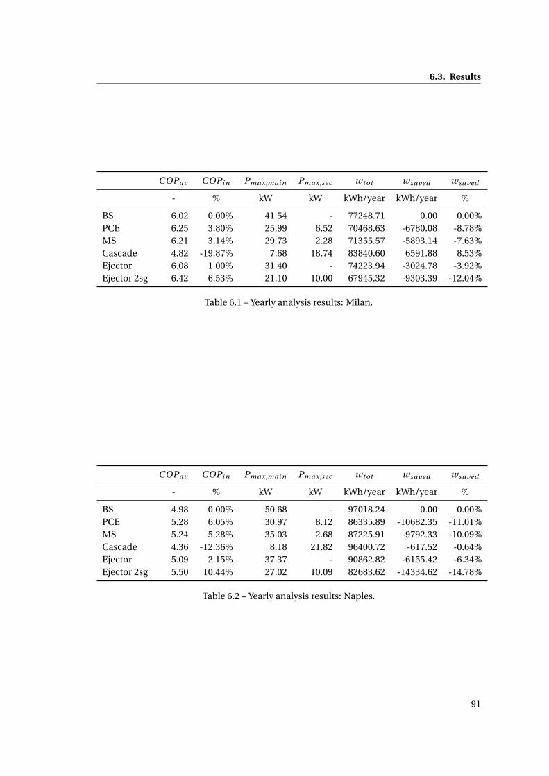
6.3. Results
COPav COPi n Pmax,mai n Pmax,sec wtot wsaved wsaved
- % kW kW kWh/year kWh/year %
BS 6.02 0.00% 41.54 - 77248.71 0.00 0.00%PCE 6.25 3.80% 25.99 6.52 70468.63 -6780.08 -8.78%MS 6.21 3.14% 29.73 2.28 71355.57 -5893.14 -7.63%Cascade 4.82 -19.87% 7.68 18.74 83840.60 6591.88 8.53%Ejector 6.08 1.00% 31.40 - 74223.94 -3024.78 -3.92%Ejector 2sg 6.42 6.53% 21.10 10.00 67945.32 -9303.39 -12.04%
Table 6.1 – Yearly analysis results: Milan.
COPav COPi n Pmax,mai n Pmax,sec wtot wsaved wsaved
- % kW kW kWh/year kWh/year %
BS 4.98 0.00% 50.68 - 97018.24 0.00 0.00%PCE 5.28 6.05% 30.97 8.12 86335.89 -10682.35 -11.01%MS 5.24 5.28% 35.03 2.68 87225.91 -9792.33 -10.09%Cascade 4.36 -12.36% 8.18 21.82 96400.72 -617.52 -0.64%Ejector 5.09 2.15% 37.37 - 90862.82 -6155.42 -6.34%Ejector 2sg 5.50 10.44% 27.02 10.09 82683.62 -14334.62 -14.78%
Table 6.2 – Yearly analysis results: Naples.
91


7 Yearly analysis: comparison with anR404A cycle
In this chapter, the last of the thesis, a comparison of the CO2 systems with a base R404A cycle
will be made. Nowadays in the countries of northern Europe several supermarket plants using
carbon dioxide as refrigeration fluid have already been installed. As said at the beginning of
the thesis the problem of a carbon dioxide cycle is working when the ambient temperature is
more then 25°C because of the low critical point. The purpose of this project is understand
if a modified system is able to achieve good performance also if is located in a zone with
hot climate condition. In the previous chapter it has been seen that the studied cycles can
improve considerably the performance compared to a base one. Now the aim is to see if
these improved systems can compete also with a system using a synthetic refrigerant. The
refrigerant chosen for the comparison is the R404A because is the most used refrigerant in
supermarket applications. R404A is a near azeotropic mixture made by 44% of R125, 52% of
R143a and 4% of R134a and its critical point is at 72.14°C and 37.35 bar. The ozone depletion
potential is zero because all its component are HFC but it has a global warming potential of
3260. Fig.7.1 shows the p-h diagram of the fluid.
7.1 R404A cycle
In this section the R404A cycle will be explain with all its own features. A new model has been
built in order to simulate the behaviour of a real R404A refrigeration system. The entire system
has been modelled based on energy and mass balance of every single component. Steady flow
energy equations and specific energy quantities have been used. The following assumptions
have been made in the analysis:
• Steady-state processes.
• Isenthalpic expansion.
• Pressure drop and heat losses are neglected.
• Isentropic efficiency for the compressor is assumed to be function of the pressure ratio
93
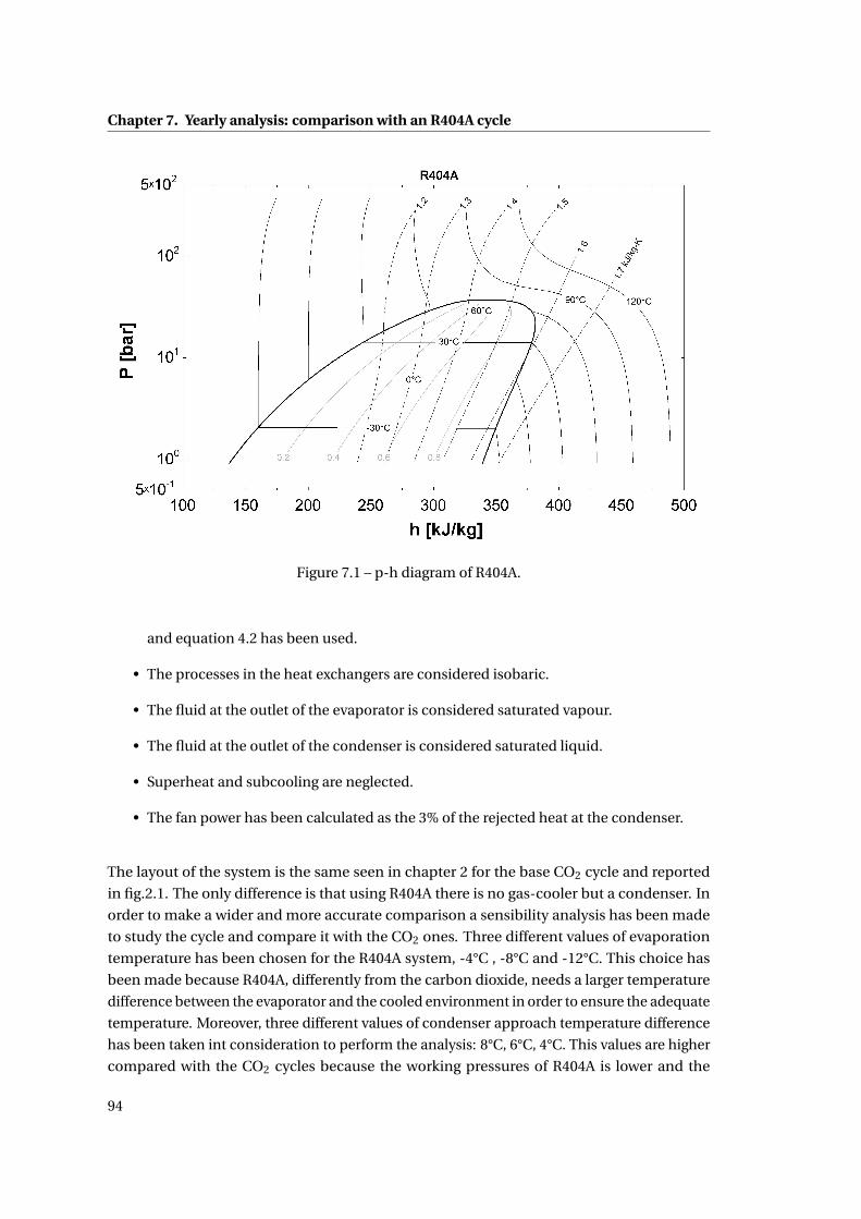
Chapter 7. Yearly analysis: comparison with an R404A cycle
Figure 7.1 – p-h diagram of R404A.
and equation 4.2 has been used.
• The processes in the heat exchangers are considered isobaric.
• The fluid at the outlet of the evaporator is considered saturated vapour.
• The fluid at the outlet of the condenser is considered saturated liquid.
• Superheat and subcooling are neglected.
• The fan power has been calculated as the 3% of the rejected heat at the condenser.
The layout of the system is the same seen in chapter 2 for the base CO2 cycle and reported
in fig.2.1. The only difference is that using R404A there is no gas-cooler but a condenser. In
order to make a wider and more accurate comparison a sensibility analysis has been made
to study the cycle and compare it with the CO2 ones. Three different values of evaporation
temperature has been chosen for the R404A system, -4°C , -8°C and -12°C. This choice has
been made because R404A, differently from the carbon dioxide, needs a larger temperature
difference between the evaporator and the cooled environment in order to ensure the adequate
temperature. Moreover, three different values of condenser approach temperature difference
has been taken int consideration to perform the analysis: 8°C, 6°C, 4°C. This values are higher
compared with the CO2 cycles because the working pressures of R404A is lower and the
94

7.2. Results
temperature is more sensitive to the pressure losses. Since it is more sensitive a certain
subcooling out of the condenser is always needed to make sure that these losses will not create
flashgas. These facts have been reported by Kim et al.[12], citing their work: "the minimum heat
rejection temperature will be lower in the CO2 cycle (compared with an ’ordinary’ refrigerant)
when heat sink inlet temperature and heat exchanger size is given. In addition, the evaporating
temperature tends to be higher for a given duty, heat source temperature, and heat exchanger
size." After have run some simulations with the Bitzer software [40] to see the limits of an
R404A compressor, the minimum condensing temperature has been setted to 15°C, 12°C
and 10°C respectively for the three evaporation temperatures. This minimum temperature
fix a minimum pressure difference through the compressor and the throttling valve that
ensure a proper functioning of the devices. Regarding the real cooling load and the ambient
temperature data, the conditions presented in chapter 6 are still valid and have been used to
model the system.
Before proceeding with the comparison of the systems, the boundary conditions and the
assumptions are summarized in the following table.
R404A cycle
Evaporative temperature -4°C, -8°C, -12°CCondenser approach temperature difference 8°C, 6°C, 4°CMinimum condensing temperature 10°C, 12°C, 15°CSubcooling and superheating 0°CCompressor isentropic efficiency polynomial, f(pressure ratio)Fan power 3% of the rejected heat
7.2 Results
The results are here presented in the following way: for each condenser approach temperature
difference two graphs and six tables are reported. The two graphs show a comparison in terms
of COP and power consumptions (with constant cooling load) between the base CO2 cycle
and the R404A cycle with different evaporative temperatures. The orange line represents the
cycle with an evaporative temperature of -4°C, the green one end the yellow one represent the
cycle with an evaporative temperature of -8°C and -12°C respectively. The tables present the
comparison in terms of yearly analysis for Milan and Naples. There are then two tables for every
combination of evaporative temperature and condenser approach. The assumptions made
for the CO2 systems are the same used for the yearly analysis in chapter 6. The results show
that the CO2 cycles are very promising compared to the R404A one. The higher performances
achieved by the carbon dioxide are due to the lower approach temperature different in the
gas-cooler/condenser and in the evaporator. The possibility to reduce these two ∆t is in
fact a great advantage that the carbon dioxide has, thanks to its thermodynamic and transfer
properties, respect to the other refrigerants.
95
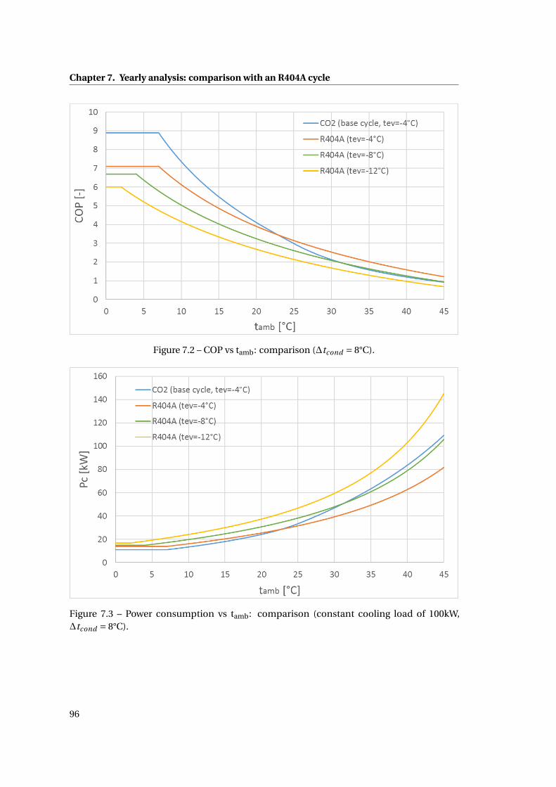
Chapter 7. Yearly analysis: comparison with an R404A cycle
Figure 7.2 – COP vs tamb: comparison (∆tcond = 8°C).
Figure 7.3 – Power consumption vs tamb: comparison (constant cooling load of 100kW,∆tcond = 8°C).
96
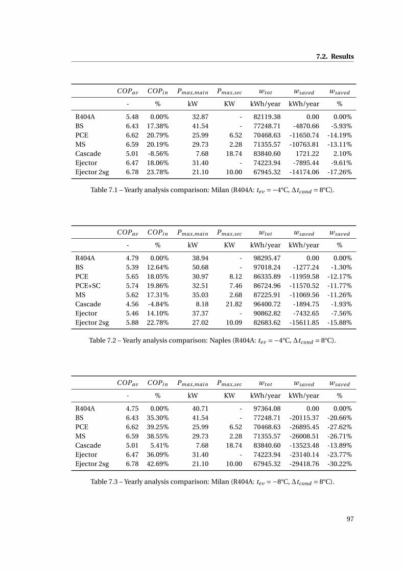
7.2. Results
COPav COPi n Pmax,mai n Pmax,sec wtot wsaved wsaved
- % kW KW kWh/year kWh/year %
R404A 5.48 0.00% 32.87 - 82119.38 0.00 0.00%BS 6.43 17.38% 41.54 - 77248.71 -4870.66 -5.93%PCE 6.62 20.79% 25.99 6.52 70468.63 -11650.74 -14.19%MS 6.59 20.19% 29.73 2.28 71355.57 -10763.81 -13.11%Cascade 5.01 -8.56% 7.68 18.74 83840.60 1721.22 2.10%Ejector 6.47 18.06% 31.40 - 74223.94 -7895.44 -9.61%Ejector 2sg 6.78 23.78% 21.10 10.00 67945.32 -14174.06 -17.26%
Table 7.1 – Yearly analysis comparison: Milan (R404A: tev =−4°C, ∆tcond = 8°C).
COPav COPi n Pmax,mai n Pmax,sec wtot wsaved wsaved
- % kW KW kWh/year kWh/year %
R404A 4.79 0.00% 38.94 - 98295.47 0.00 0.00%BS 5.39 12.64% 50.68 - 97018.24 -1277.24 -1.30%PCE 5.65 18.05% 30.97 8.12 86335.89 -11959.58 -12.17%PCE+SC 5.74 19.86% 32.51 7.46 86724.96 -11570.52 -11.77%MS 5.62 17.31% 35.03 2.68 87225.91 -11069.56 -11.26%Cascade 4.56 -4.84% 8.18 21.82 96400.72 -1894.75 -1.93%Ejector 5.46 14.10% 37.37 - 90862.82 -7432.65 -7.56%Ejector 2sg 5.88 22.78% 27.02 10.09 82683.62 -15611.85 -15.88%
Table 7.2 – Yearly analysis comparison: Naples (R404A: tev =−4°C, ∆tcond = 8°C).
COPav COPi n Pmax,mai n Pmax,sec wtot wsaved wsaved
- % kW KW kWh/year kWh/year %
R404A 4.75 0.00% 40.71 - 97364.08 0.00 0.00%BS 6.43 35.30% 41.54 - 77248.71 -20115.37 -20.66%PCE 6.62 39.25% 25.99 6.52 70468.63 -26895.45 -27.62%MS 6.59 38.55% 29.73 2.28 71355.57 -26008.51 -26.71%Cascade 5.01 5.41% 7.68 18.74 83840.60 -13523.48 -13.89%Ejector 6.47 36.09% 31.40 - 74223.94 -23140.14 -23.77%Ejector 2sg 6.78 42.69% 21.10 10.00 67945.32 -29418.76 -30.22%
Table 7.3 – Yearly analysis comparison: Milan (R404A: tev =−8°C, ∆tcond = 8°C).
97

Chapter 7. Yearly analysis: comparison with an R404A cycle
COPav COPi n Pmax,mai n Pmax,sec wtot wsaved wsaved
- % kW KW kWh/year kWh/year %
R404A 4.00 0.00% 48.50 - 118492.35 0.00 0.00%BS 5.39 34.87% 50.68 - 97018.24 -21474.11 -18.12%PCE 5.65 41.35% 30.97 8.12 86335.89 -32156.46 -27.14%MS 5.62 40.46% 35.03 2.68 87225.91 -31266.44 -26.39%Cascade 4.56 13.94% 8.18 21.82 96400.72 -22091.63 -18.64%Ejector 5.46 36.62% 37.37 - 90862.82 -27629.53 -23.32%Ejector 2sg 5.88 47.01% 27.02 10.09 82683.62 -35808.73 -30.22%
Table 7.4 – Yearly analysis comparison: Naples (R404A: tev =−8°C, ∆tcond = 8°C).
COPav COPi n Pmax,mai n Pmax,sec wtot wsaved wsaved
- % kW KW kWh/year kWh/year %
R404A 4.01 0.00% 51.52 - 117532.53 0.00 0.00%BS 6.43 60.52% 41.54 - 77248.71 -40283.81 -34.27%PCE 6.62 65.20% 25.99 6.52 70468.63 -47063.89 -40.04%MS 6.59 64.38% 29.73 2.28 71355.57 -46176.96 -39.29%Cascade 5.01 25.05% 7.68 18.74 83840.60 -33691.93 -28.67%Ejector 6.47 61.46% 31.40 - 74223.94 -43308.59 -36.85%Ejector 2sg 6.78 69.28% 21.10 10.00 67945.32 -49587.21 -42.19%
Table 7.5 – Yearly analysis comparison: Milan (R404A: tev =−12°C, ∆tcond = 8°C).
COPav COPi n Pmax,mai n Pmax,sec wtot wsaved wsaved
- % kW KW kWh/year kWh/year %
R404A 3.30 0.00% 62.03 - 144287.32 0.00 0.00%BS 5.39 63.30% 50.68 - 97018.24 -47269.08 -32.76%PCE 5.65 71.14% 30.97 8.12 86335.89 -57951.43 -40.16%MS 5.62 70.06% 35.03 2.68 87225.91 -57061.41 -39.55%Cascade 4.56 37.96% 8.18 21.82 96400.72 -47886.60 -33.19%Ejector 5.46 65.41% 37.37 - 90862.82 -53424.50 -37.03%Ejector 2sg 5.88 77.99% 27.02 10.09 82683.62 -61603.70 -42.70%
Table 7.6 – Yearly analysis comparison: Naples (R404A: tev =−12°C, ∆tcond = 8°C).
98

7.2. Results
Figure 7.4 – COP vs tamb: comparison (∆tcond = 6°C).
Figure 7.5 – Power consumption vs tamb: comparison (constant cooling load of 100kW,∆tcond = 6°C).
99

Chapter 7. Yearly analysis: comparison with an R404A cycle
COPav COPi n Pmax,mai n Pmax,sec wtot wsaved wsaved
- % kW KW kWh/year kWh/year %
R404A 5.48 0.00% 29.85 - 76585.67 0.00 0.00%BS 6.02 9.81% 41.54 - 77248.71 663.05 0.87%PCE 6.25 13.98% 25.99 6.52 70468.63 -6117.03 -7.99%MS 6.21 13.26% 29.73 2.28 71355.57 -5230.10 -6.83%Cascade 4.82 -12.02% 7.678 18.74 83840.60 7254.93 9.47%Ejector 6.08 10.90% 31.4 - 74223.94 -2361.73 -3.08%Ejector 2sg 6.42 16.98% 21.1 10.00 67945.32 -8640.35 -11.28%
Table 7.7 – Yearly analysis comparison: Naples (R404A: tev =−4°C, ∆tcond = 6°C).
COPav COPi n Pmax,mai n Pmax,sec wtot wsaved wsaved
- % kW KW kWh/year kWh/year %
R404A 4.87 0.00% 35.30 - 90420.31 0.00 0.00%BS 4.98 2.32% 50.68 - 97018.24 6597.92 7.30%PCE 5.28 8.52% 30.97 8.12 86335.89 -4084.43 -4.52%MS 5.24 7.72% 35.03 2.68 87225.91 -3194.41 -3.53%Cascade 4.36 -10.33% 8.182 21.82 96400.72 5980.41 6.61%Ejector 5.09 4.52% 37.37 - 90862.82 442.51 0.49%Ejector 2sg 5.50 13.00% 27.02 10.09 82683.62 -7736.69 -8.56%
Table 7.8 – Yearly analysis comparison: Naples (R404A: tev =−4°C, ∆tcond = 6°C).
COPav COPi n Pmax,mai n Pmax,sec wtot wsaved wsaved
- % kW KW kWh/year kWh/year %
R404A 4.77 0.00% 36.84 - 90189.54 0.00 0.00%BS 6.02 26.18% 41.54 - 77248.71 -12940.83 -14.35%PCE 6.25 30.97% 25.99 6.52 70468.63 -19720.91 -21.87%MS 6.21 30.14% 29.73 2.28 71355.57 -18833.97 -20.88%Cascade 4.82 1.10% 7.678 18.74 83840.60 -6348.94 -7.04%Ejector 6.08 27.44% 31.4 - 74223.94 -15965.60 -17.70%Ejector+BP 6.42 34.42% 21.1 10.00 67945.32 -22244.22 -24.66%
Table 7.9 – Yearly analysis comparison: Naples (R404A: tev =−8°C, ∆tcond = 6°C).
100

7.2. Results
COPav COPi n Pmax,mai n Pmax,sec wtot wsaved wsaved
- % kW KW kWh/year kWh/year %
R404A 4.09 0.00% 43.76 - 108593.93 0.00 0.00%BS 4.98 21.85% 50.68 - 97018.24 -11575.69 -10.66%PCE 5.28 29.22% 30.97 8.12 86335.89 -22258.04 -20.50%MS 5.24 28.28% 35.03 2.68 87225.91 -21368.02 -19.68%Cascade 4.36 6.78% 8.182 21.82 96400.72 -12193.21 -11.23%Ejector 5.09 24.47% 37.37 - 90862.82 -17731.11 -16.33%Ejector+BP 5.50 34.57% 27.02 10.09 82683.62 -25910.31 -23.86%
Table 7.10 – Yearly analysis comparison: Naples (R404A: tev =−8°C, ∆tcond = 6°C).
COPav COPi n Pmax,mai n Pmax,sec wtot wsaved wsaved
- % kW KW kWh/year kWh/year %
R404A 4.04 0.00% 46.29 - 108268.02 0.00 0.00%BS 6.02 49.10% 41.54 - 77248.71 -31019.31 -28.65%PCE 6.25 54.76% 25.99 6.52 70468.63 -37799.39 -34.91%MS 6.21 53.78% 29.73 2.28 71355.57 -36912.45 -34.09%Cascade 4.82 19.47% 7.678 18.74 83840.60 -24427.42 -22.56%Ejector 6.08 50.59% 31.4 - 74223.94 -34044.08 -31.44%Ejector+BP 6.42 58.84% 21.1 10.00 67945.32 -40322.70 -37.24%
Table 7.11 – Yearly analysis comparison: Naples (R404A: tev =−12°C, ∆tcond = 6°C).
COPav COPi n Pmax,mai n Pmax,sec wtot wsaved wsaved
- % kW KW kWh/year kWh/year %
R404A 3.38 0.00% 55.46 - 131833.00 0.00 0.00%BS 4.98 47.24% 50.68 - 97018.24 -34814.76 -26.41%PCE 5.28 56.15% 30.97 8.12 86335.89 -45497.11 -34.51%MS 5.24 55.01% 35.03 2.68 87225.91 -44607.09 -33.84%Cascade 4.36 29.03% 8.182 21.82 96400.72 -35432.28 -26.88%Ejector 5.09 50.41% 37.37 - 90862.82 -40970.18 -31.08%Ejector+BP 5.50 62.60% 27.02 10.09 82683.62 -49149.38 -37.28%
Table 7.12 – Yearly analysis comparison: Naples (R404A: tev =−12°C, ∆tcond = 6°C).
101

Chapter 7. Yearly analysis: comparison with an R404A cycle
COPav COPi n Pmax,mai n Pmax,sec wtot wsaved wsaved
- % kW KW kWh/year kWh/year %
R404A 5.75 0.00% 27.13 - 71782.31 0.00 0.00%BS 6.02 4.69% 41.54 - 77248.71 5466.41 7.62%PCE 6.25 8.66% 25.99 6.52 70468.63 -1313.67 -1.83%MS 6.21 7.98% 29.73 2.28 71355.57 -426.74 -0.59%Cascade 4.82 -16.12% 7.678 18.74 83840.60 12058.29 16.80%Ejector 6.08 5.73% 31.4 - 74223.94 2441.63 3.40%Ejector+BP 6.42 11.53% 21.1 10.00 67945.32 -3836.99 -5.35%
Table 7.13 – Yearly analysis comparison: Naples (R404A: tev =−4°C, ∆tcond = 4°C).
COPav COPi n Pmax,mai n Pmax,sec wtot wsaved wsaved
- % kW KW kWh/year kWh/year %
R404A 5.22 0.00% 32.05 - 83496.26 0.00 0.00%BS 4.98 -4.62% 50.68 - 97018.24 13521.97 16.19%PCE 5.28 1.16% 30.97 8.12 86335.89 2839.62 3.40%MS 5.24 0.42% 35.03 2.68 87225.91 3729.64 4.47%Cascade 4.36 -16.41% 8.182 21.82 96400.72 12904.46 15.46%Ejector 5.09 -2.56% 37.37 - 90862.82 7366.56 8.82%Ejector+BP 5.50 5.34% 27.02 10.09 82683.62 -812.64 -0.97%
Table 7.14 – Yearly analysis comparison: Naples (R404A: tev =−4°C, ∆tcond = 4°C).
COPav COPi n Pmax,mai n Pmax,sec wtot wsaved wsaved
- % kW KW kWh/year kWh/year %
R404A 5.04 0.00% 33.39 - 83925.27 0.00 0.00%BS 6.02 19.43% 41.54 - 77248.71 -6676.55 -7.96%PCE 6.25 23.96% 25.99 6.52 70468.63 -13456.64 -16.03%MS 6.21 23.18% 29.73 2.28 71355.57 -12569.70 -14.98%Cascade 4.82 -4.31% 7.678 18.74 83840.60 -84.67 -0.10%Ejector 6.08 20.62% 31.4 - 74223.94 -9701.33 -11.56%Ejector+BP 6.42 27.23% 21.1 10.00 67945.32 -15979.95 -19.04%
Table 7.15 – Yearly analysis comparison: Naples (R404A: tev =−8°C, ∆tcond = 4°C).
102

7.2. Results
Figure 7.6 – COP vs tamb: comparison (∆tcond = 4°C).
Figure 7.7 – Power consumption vs tamb: comparison (constant cooling load of 100kW,∆tcond = 4°C).
103

Chapter 7. Yearly analysis: comparison with an R404A cycle
COPav COPi n Pmax,mai n Pmax,sec wtot wsaved wsaved
- % kW KW kWh/year kWh/year %
R404A 4.43 0.00% 39.58 - 99743.43 0.00 0.00%BS 4.98 12.53% 50.68 - 97018.24 -2725.19 -2.73%PCE 5.28 19.34% 30.97 8.12 86335.89 -13407.54 -13.44%MS 5.24 18.47% 35.03 2.68 87225.91 -12517.52 -12.55%Cascade 4.36 -1.39% 8.182 21.82 96400.72 -3342.71 -3.35%Ejector 5.09 14.95% 37.37 - 90862.82 -8880.61 -8.90%Ejector+BP 5.50 24.27% 27.02 10.09 82683.62 -17059.80 -17.10%
Table 7.16 – Yearly analysis comparison: Naples (R404A: tev =−8°C, ∆tcond = 4°C).
COPav COPi n Pmax,mai n Pmax,sec wtot wsaved wsaved
- % kW KW kWh/year kWh/year %
R404A 4.29 0.00% 41.71 - 100224.10 0.00 0.00%BS 6.02 40.32% 41.54 - 77248.71 -22975.39 -22.92%PCE 6.25 45.65% 25.99 6.52 70468.63 -29755.47 -29.69%MS 6.21 44.73% 29.73 2.28 71355.57 -28868.53 -28.80%Cascade 4.82 12.43% 7.678 18.74 83840.60 -16383.50 -16.35%Ejector 6.08 41.72% 31.4 - 74223.94 -26000.16 -25.94%Ejector+BP 6.42 49.49% 21.1 10.00 67945.32 -32278.78 -32.21%
Table 7.17 – Yearly analysis comparison: Naples (R404A: tev =−12°C, ∆tcond = 4°C).
COPav COPi n Pmax,mai n Pmax,sec wtot wsaved wsaved
- % kW KW kWh/year kWh/year %
R404A 3.68 0.00% 49.79 - 120682.17 0.00 0.00%BS 4.98 35.33% 50.68 - 97018.24 -23663.93 -19.61%PCE 5.28 43.52% 30.97 8.12 86335.89 -34346.28 -28.46%MS 5.24 42.47% 35.03 2.68 87225.91 -33456.26 -27.72%Cascade 4.36 18.60% 8.182 21.82 96400.72 -24281.45 -20.12%Ejector 5.09 38.24% 37.37 - 90862.82 -29819.35 -24.71%Ejector+BP 5.50 49.45% 27.02 10.09 82683.62 -37998.55 -31.49%
Table 7.18 – Yearly analysis comparison: Naples (R404A: tev =−12°C, ∆tcond = 4°C).
104

8 Conclusions
During the last decades the industry of refrigeration and air-conditioning had to face some
radical changes due to the increasing concern about the health of our planet. CFC and HCFC
fluids have been discovered to be very harmful and dangerous for the ozone layer and they
have been banned already. Even HFCs, introduced as replacements, are now discussion topic
because of their impact on the global warming. Regulation (EU) 517/2014 of the European
Parliament has been approved with the purpose to put them out of the market in the next years.
Natural refrigerants and HFOs, a new type of synthetic fluids, seem now the only solution to
reduce the human impact on the environment. Research on natural refrigerants is growing on
many parallel ways, including the use of hydrocarbons and ammonia by minimizing charge to
avoid safety problem due to their toxicity and flammability. This thesis is focused on carbon
dioxide, a natural refrigerant that like most of others has no ozone depletion potential and
negligible global warming potential. CO2 was already used during the end of the 19th century
and beginning of the 20th as a refrigerant. From the middle of the 20th century carbon dioxide
was completely abandoned due to appearance of CFCs in the market. After the discovery
of the damages that these synthetic fluids can do to our planet the reborn of CO2 started.
Thermodynamic and transport properties of carbon dioxide are favourable in terms of heat
transfer and pressure drop. It has high working pressure but the main disadvantage is the
low critical temperature. Because of this the heat rejection will in most cases take place
in supercritical region. This makes the cycle working as transcritical. The higher average
temperature of heat rejection and the larger throttling loss penalize the basic CO2 cycle
compared to other refrigerants. Four different solutions have been taken into consideration in
order to decrease these losses: parallel compression with and without recooler, mechanical
subcooling, cascade system and the use of an ejector to recover the expansion work, with single
and parallel compression. From a design condition point of view (a constant and very high
ambient temperature has been chosen) it has been proved that all the systems achieve better
performances than the base cycle. The cascade system using R134a as secondary fluid permits
to reduce the power consumption by 39%, followed by the cycle with mechanical subcooling
( 24% ) and the ejector cycle with parallel compression (22%). These results are interesting
and offer a good overview of the adoptable possibilities to improve the base cycle when used
105

Chapter 8. Conclusions
in hot climate. However they do not take into account the fact that a refrigeration system is
subject to very different climate conditions during a year of operation. The second and main
part of the present study is focused on the yearly analysis of the previously mentioned cycles.
Two different Italian cities have been chosen to perform the analysis: Milan and Naples. A
Test Reference Year (TRY) dataset has been used to describe the ambient temperature over
the year. This choice permitted to study the system under two different climate conditions.
A plant installed in Milan works in transcritical mode for 601 hours a year versus 1095 for
a plant installed in Naples. Accurate and realistic assumptions have been made to model
the cycles. Using an ejector cycle with two suction groups (parallel compression) leads to
an energy saving of 12.0% and 14.8% respectively in Milan and Naples compared to the base
cycle consumptions. The parallel compression economization system shows satisfying results
as well, with an energy saving of 8.8% and 11.0% for the two cities respectively. The cascade
system, best cycle when dealing with high ambient temperature, in the yearly analysis is the
one with the lowest performances. The last part of the project proposes a simple comparison
between the CO2 systems and a R404A cycle. Results are interesting and show that carbon
dioxide can also be competitive where the climate conditions are not favourable. Different
trial plants have been installed in southern Europe already. The real data that can be obtained
thanks to these systems will be fundamental to understand if the CO2 can really replace the
synthetic refrigerants and finally reduce the impact that the human activity is having on the
climate.
106

Bibliography
[1] International Energy Agency. World Energy Outlook. 2015.
[2] L. Lucas. IIR news. International Journal of Refrigeration, 21(2):87–88, 1998.
[3] Regulation (ec) no 2037/2000 of the European Parliament and the council of 29 June 2000
on substances that deplete the ozone layer. Official Journal of the European Communities,
244:1–24, 2000.
[4] V. Sharma, B. Fricke, and P. Bansal. Comparative analysis of various CO2 configurations
in supermarket refrigeration systems. International Journal of Refrigeration, 46:86–99,
2014.
[5] S. Klein and F. Alvarado. Engineering equation solver. F-Chart Software. 2001.
[6] R. Span and W. Wagner. A new equation of state for carbon dioxide covering the fluid
region from the triple-point temperature to 1100 K at pressure up to 800 MPa. Journal of
Physical and Chemical Reference Data, 26:1509–96, 1996.
[7] A. Pearson. Carbon dioxide - New uses for an old refrigerant. International Journal of
Refrigeration, 28(8):1140–1148, 2005.
[8] J. M. Calm. The next generation of refrigerants - Historical review, considerations, and
outlook. International Journal of Refrigeration, 31(7):1123–1133, 2008.
[9] G. Lorentzen. Carbon dioxide as a refrigerant. Journal of the Franklin Institute, 196(5):
713, 1993.
[10] G. Lorentzen. The use of natural refrigerants : a complete solution to the CFC/HCFC
predicament . International Journal of Refrigeration, 18(3):190–197, 1995.
[11] G. Lorentzen. Trans-critical vapour compression cycle device, Patent No. WO/07683.
1990.
[12] M. Kim. Fundamental process and system design issues in CO2 vapor compression systems,
volume 30. 2004.
107

Bibliography
[13] A. Bredesen, A. Hafner, and J. Pettersen. Heat transfer and pressure drop for in-tube evap-
oration of CO2. International Conference on Heat Transfer Issues in Natural Refrigerants,
College Park, MD, pages 1–15, 1997.
[14] S. Girotto, S. Minetto, and P. Neksa. Commercial refrigeration system using CO2 as the
refrigerant. International Journal of Refrigeration, 27:717–723, 2004.
[15] S. Sawalha, M. Karampour, and J. Rogstam. Field measurements of supermarket refrigera-
tion systems. Part I: Analysis of CO2 trans-critical refrigeration systems. Applied Thermal
Engineering, 87:633–647, 2015.
[16] S. M. Liao, T. S. Zhao, and A. Jakobsen. Correlation of optimal heat rejection pressures in
transcritical carbon dioxide cycles. Applied Thermal Engineering, 20(9):831–841, 2000.
[17] Y. T. Ge and S. A. Tassou. Thermodynamic analysis of transcritical CO2 booster refriger-
ation systems in supermarket. Energy Conversion and Management, 52(4):1868–1875,
2011.
[18] J. Sarkar. Performance characteristics of refrigeration cycle with parallel compression
economization. International Journal of Energy Research, 34(13):1205–1214, 2010.
[19] J. Sarkar and N. Agrawal. Performance optimization of transcritical CO2 cycle with parallel
compression economization. International Journal of Thermal Science, 49:838–843, 2009.
[20] S. M. Zubair. Improvement of refrigeration/air-conditioning performance with mechani-
cal sub-cooling. Energy, 15(5):427–433, 1990.
[21] S. M. Zubair. Thermodynamics of a vapor-compression refrigeration cycle with mechani-
cal subcooling. Energy, 19(6):707–715, 1994.
[22] J. Khan and S. Zubair. Design and rating of an integrated mechanical-subcooling vapor-
compression refrigeration system. Energy Conversion and Management, 41(11):1201–
1222, 2000.
[23] J. W. Thornton, S. A. Klein, and J. W. Mitchell. Dedicated mechanical subcoolmg design
strategies for supermarket a kations. International Journal of Refrigeration, 17(8):508–515,
1994.
[24] J. Khan and S. M. Zubair. Design and rating of dedicated mechanical-subcooling vapour
compression refrigeration systems. Proceedings of the Institution of Mechanical Engineers,
Part A: Journal of Power and Energy, 214(5):455–471, 2000.
[25] R. Llopis, R. Cabello, D. Sánchez, and E. Torrella. Energy improvements of CO2 transcriti-
cal refrigeration cycles using dedicated mechanical subcooling. International Journal of
Refrigeration, 55:129–141, 2015.
108

Bibliography
[26] C. Sanz-Kock, R. Llopis, D. Sánchez, R. Cabello, and E. Torrella. Experimental evaluation
of a R134a/CO2 cascade refrigeration plant. Applied Thermal Engineering, 73(1):39–48,
2014.
[27] A. Da Silva, E.P. Bandarra Filho, and A.H.P. Antunes. Comparison of a R744 cascade
refrigeration system with R404A and R22 conventional systems for supermarkets. Applied
Thermal Engineering, 41:30–35, 2012.
[28] S. Bhattacharyya, S. Mukhopadhyay, A. Kumar, R. K. Khurana, and J. Sarkar. Optimization
of a CO2-C3H8 cascade system for refrigeration and heating. International Journal of
Refrigeration, 28(8):1284–1292, 2005.
[29] H. Tian, Y. Ma, M. Li, and W. Wang. Study on expansion power recovery in CO2 trans-
critical cycle. Energy Conversion and Management, 51(12):2516–2522, 2010.
[30] Y.F. Liu and G.Y. Jin. Vortex tube expansion two-stage transcritical CO2 refrigeration cycle.
Advanced Materials Research, 516:1219–1223, 2012.
[31] D. Li and E.A. Groll. Transcritical CO2 refrigeration cycle with ejector-expansion device.
International Journal of Refrigeration, 28(5):766–773, 2005.
[32] S. Fangtian and M. Yitai. Thermodynamic analysis of transcritical CO2 refrigeration cycle
with an ejector. Applied Thermal Engineering, 31(6-7):1184–1189, 2011.
[33] H. K. Ersoy and N. Bilir. Performance characteristics of ejector expander transcritical
CO2 refrigeration cycle. Proceedings of the Institution of Mechanical Engineers, Part A:
Journal of Power and Energy, 226(5):623–635, 2012.
[34] E. Kriezi, K. Fredslund, K. Banasiak, and A. Hafner. Multi ejector and the impact of ejector
design on the operation of a CO2 refrigeration System. 2015.
[35] Kornhauser. The Use Of An Ejector In A Geothermal Flash System. Proceedings of the
25th Intersociety Energy Conversion Engineering Conference, 5, 1990.
[36] S. Elbel. Historical and present developments of ejector refrigeration systems with
emphasis on transcritical carbon dioxide air-conditioning applications. International
Journal of Refrigeration, 34(7):1545–1561, 2011.
[37] F. Liu and E.A. Groll. Study of ejector efficiencies in refrigeration cycles. Applied Thermal
Engineering, 52(2):360–370, 2013.
[38] F. Liu, E. Groll, and D. Li. Investigation on performance of variable geometry ejectors for
CO 2 refrigeration cycles. Energy, 45(1):829–839, 2012.
[39] Private person. Kristian Fredslund, refrigeration specialist, DANFOSS.
[40] BITZER Group. Bitzer compressors database. 2015. URL https://www.bitzer.de/
websoftware/.
109

Bibliography
[41] National Institute of Standards U.S. department of Commerce and Technology. NIST
Reference Fluid Thermodynamic and Transport Properties Database, REFPROP. URL
http://www.nist.gov/srd/nist23.cfm.
[42] S. Girotto, S. Minetto, and M. Salvatore. Recent installations of CO2 supermarket refriger-
ation system for warm climates: data from the field. Science et Technique du Froid, 2014
(1):78–85, 2014.
[43] U.S. department of Energy. Energy Plus, Italian weather data, 2015. URL https:
//energyplus.net/weather-region/europe_wmo_region_6/ITA%20%20.
110

A Appendix A
This appendix collects the models used to perform the yearly analysis for every cycles. The
models have been written using the equation solver EES [5]. Every model has been built
following some simple steps. The code starts with a procedure that fix the condenser/gas
cooler operation, this part is similar for all the cycles except for the equation that optimize the
gas cooler pressure. In this procedure the minimum condensing temperature is set using an
IF/THEN/ELSE cycle. Another one is used to fix the conditions when to pass from subcritical to
transcritical operation. One more procedure have been used to set the load and the respective
variation with the ambient temperature and the hour of the day. After this all the boundary
conditions are set, except for the ambient temperature and the hour of the day that are the
entrance data in the parametric table. The main part of the model is made by all the equations
that fix the points and the features of the cycle. At the end the parameters that show the results
are calculated. The complete model of the base CO2 cycle is reported in the appendix. For the
other systems only the main parts that differ from the first one are presented. It’s important to
say that in order to skip the secondary compressor in the parallel compression economization
cycle a filter in the results has been used. In this way it was possible to make the code lighter
and the compilation faster. The same procedure has been used for the normal ejector cycle
and for the ejector cycle with two suction groups.
A.1 Base cycle
"CONDENSER/GAS COOLER"
PROCEDURE CONDENSER
"SUBCRITICAL OPERATION"
IF Tamb<7.05 THEN
tcond=10
pc=pressure(R$,t=tcond,x=0)
p[2]=pc
h_is[2]=enthalpy(R$,p=p[2],s=s[1])
"eta_is=((h_is[2]-h[1])/(h[2]-h[1]))"
111

Appendix A
h[2]=((h_is[2]-h[1])/eta_is)+h[1]
s[2]=entropy(R$,p=p[2],h=h[2])
t[2]=temperature(R$,p=p[2],h=h[2])
p[3]=p[2]
t[3]=temperature(R$,p=p[3],x=0)
h[3]=enthalpy(R$,p=p[3],x=0)
s[3]=entropy(R$,p=p[3],x=0)
tgc_out=0
ELSE
IF Tamb<25.15 THEN
tcond=tamb+3
pc=pressure(R$,t=tcond,x=0)
p[2]=pc
h_is[2]=enthalpy(R$,p=p[2],s=s[1])
h[2]=((h_is[2]-h[1])/eta_is)+h[1]
s[2]=entropy(R$,p=p[2],h=h[2])
t[2]=temperature(R$,p=p[2],h=h[2])
p[3]=p[2]
t[3]=temperature(R$,p=p[3],x=0)
h[3]=enthalpy(R$,p=p[3],x=0)
s[3]=entropy(R$,p=p[3],x=0)
tgc_out=0
ELSE
"TRANSCRITICAL OPERATION ("Tamb>25.15")"
tgc_out=tamb+3
pc=(2.778-0.0157*te)*tgc_out+(0.381*te-9.34)
p[2]=pc
h_is[2]=enthalpy(R$,p=p[2],s=s[1])
h[2]=((h_is[2]-h[1])/eta_is)+h[1]
t[2]=temperature(R$,p=p[2],h=h[2])
s[2]=entropy(R$,p=p[2],t=t[2])
p[3]=p[2]
t[3]=Tgc_out
h[3]=enthalpy(R$,p=p[3],t=t[3])
s[3]=entropy(R$,p=p[3],t=t[3])
tcond=0
ENDIF
ENDIF
END
"LOAD"
PROCEDURE LOAD
"LOAD IN FUNCTION OF AMBIENT TEMPERATURE"
112

A.1. Base cycle
IF Tamb>15 THEN
P_ev_real_d=(1/55)*tamb*P_ev+(5/22)*P_ev
P_ev_real_n=0.6*P_ev_real_d
ELSE
P_ev_real_d=0.5*P_ev
P_ev_real_n=0.6*P_ev_real_d
ENDIF
"DAY/NIGHT LOAD"
IF (h>7) AND (h<20) THEN
P_ev_real=P_ev_real_d
ELSE
P_ev_real=P_ev_real_n
ENDIF
END
"CYCLE MODELLING, MAIN PART"
R$=’R744’
"BOUNDARY CONDITION"
te=-4
eta_is=1.003-0.121*(pc/pe)
SH=0.00001
P_ev=100 "@ 100% load"
CALL LOAD
"CYCLE ANALYSIS"
t[1]=te
pe=pressure(R$,t=t[1],x=1)
p[1]=pe
h[1]=enthalpy(R$,p=p[1],t=t[1]+SH)
s[1]=entropy(R$,p=p[1],t=t[1]+SH)
CALL CONDENSER
p[4]=p[1]
h[4]=h[3]
s[4]=entropy(R$,p=p[4],h=h[4])
t[4]=t[1]
x[4] = quality(R$,p=p[4],h=h[4])
Q_dot_ev=(h[1]-h[4])
Q_dot_gc=(h[3]-h[2])
W_dot_tot=(h[2]-h[1])
COP=((h[1]-h[4])/((h[2]-h[1])-0.03*(h[3]-h[2])))
COP_p=(h[1]-h[4])/(h[2]-h[1])
m_dot=P_ev_real/Q_dot_ev
P_comp=m_dot*W_dot_tot
P_vent=-0.03*m_dot*(h[3]-h[2])
113

Appendix A
A.2 Parallel compression economization
The equations used to optimize the gas cooler pressure and the economizer pressure are:
pc=2.54*tgc_out-4.25
peco=0.4615*tamb+35.3846
"CYCLE MODELLING, MAIN PART"
eta_is_main=1.003-0.121*(pc/pe)
eta_is_sec=1.003-0.121*(pc/peco)
t[1]=te
pe=pressure(R$,t=t[1],x=1)
p[1]=pe
h[1]=enthalpy(R$,p=p[1],t=t[1]+SH)
s[1]=entropy(R$,p=p[1],t=t[1]+SH)
CALL CONDENSER p[4]=peco
h[4]=h[3]
s[4]=entropy(R$,p=p[4],h=h[4])
teco=temperature(R$,p=p[4],h=h[4])
t[4]=teco
x[4] = quality(R$,p=p[4],h=h[4])
x[4]=y_flash
(1-x[4])=y_ev
p[5]=p[4]
t[5]=t[4]
h[5]=enthalpy(R$,p=p[5],x=0)
s[5]=entropy(R$,p=p[5],x=0)
p[6]=pe
h[6]=h[5]
x[6] = quality(R$,p=p[6],h=h[6])
s[6]=entropy(R$,p=p[6],h=h[6])
t[6]=te
p[7]=peco
t[7]=t[4]
h[7]=enthalpy(R$,p=p[7],t=t[7]+SH)
s[7]=entropy(R$,p=p[7],t=t[7]+SH)
v[7]=volume(R$,p=p[7],t=t[7]+SH)
p[8]=pc
h_is[8]=enthalpy(R$,p=p[8],s=s[7])
eta_is_sec=((h_is[8]-h[7])/(h[8]-h[7]))
114

A.3. Parallel compression economization with recooler
t[8]=temperature(R$,p=p[8],h=h[8])
s[8]=entropy(R$,p=p[8],t=t[8])
y_flash*h[8]+y_ev*h[2]=h[9]
p[9]=pc
t[9]=temperature(R$,p=p[9],h=h[9])
s[9]=entropy(R$,p=p[9],h=h[9])
Q_dot_ev=y_ev*(h[1]-h[6])
Q_dot_gc=(h[3]-h[9])
W_dot_tot=y_ev*(h[2]-h[1])+y_flash*(h[8]-h[7])
COP=Q_dot_ev/(W_dot_tot-0.03*Q_dot_gc)
COP_p=P_ev_real/P_comp
m_dot_tot=P_ev_real/Q_dot_ev
P_comp=m_dot_tot*W_dot_tot
P_comp_main=m_dot_tot*y_ev*(h[2]-h[1])
P_comp_sec=m_dot_tot*y_flash*(h[8]-h[7])
m_vol=m_dot_tot*y_flash*v[7]
P_vent=-0.03*m_dot_tot*(h[3]-h[9])
A.3 Parallel compression economization with recooler
The equations used to optimize the gas cooler pressure and the subcooler pressure are:
psc=0.4615*tamb+35.3846
pc=2.58*tgc_out-5.71
"CYCLE MODELLING, MAIN PART"
eta_is_main=1.003-0.121*(pc/pe)
eta_is_sec=1.003-0.121*(pc/psc)
y=1
eta_sc=0.7
t[1]=te
pe=pressure(R$,t=t[1],x=1)
p[1]=pe
h[1]=enthalpy(R$,p=p[1],t=t[1]+SH)
s[1]=entropy(R$,p=p[1],t=t[1]+SH)
CALL CONDENSER
p[4]=psc
h[4]=h[3]
s[4]=entropy(R$,p=p[4],h=h[4])
tsc=temperature(R$,p=p[4],h=h[4])
t[4]=tsc
115

Appendix A
x[4] = quality(R$,p=p[4],h=h[4])
p[5]=psc
t[5]=t[4]
h[5]=enthalpy(R$,p=p[5],t=t[5]+SH)
s[5]=entropy(R$,p=p[5],t=t[5]+SH)
p[6]=pc
h_is[6]=enthalpy(R$,p=p[6],s=s[5])
eta_is_sec=((h_is[6]-h[5])/(h[6]-h[5]))
t[6]=temperature(R$,p=p[6],h=h[6])
s[6]=entropy(R$,p=p[6],t=t[6])
y=y_sc+y_ev
y_sc*h[6]+y_ev*h[2]=y*h[7]
p[7]=pc
t[7]=temperature(R$,p=p[7],h=h[7])
s[7]=entropy(R$,p=p[7],h=h[7])
eta_sc=(t[3]-t[8])/(t[3]-t[4])
p[8]=pc
h[8]=enthalpy(R$,p=p[8],t=t[8])
s[8]=entropy(R$,p=p[8],t=t[8])
p[9]=pe
h[9]=h[8]
x[9]=quality(R$,p=p[9],h=h[9])
s[9]=entropy(R$,p=p[9],h=h[9])
t[9]=te
Q_dot_sc=(h[3]-h[8])*y_ev
Q_dot_sc=(h[5]-h[4])*y_sc
Q_dot_ev=y_ev*(h[1]-h[9])
Q_dot_gc=y*(h[3]-h[7])
W_dot_tot=y_ev*(h[2]-h[1])+y_sc*(h[6]-h[5])
COP=Q_dot_ev/(W_dot_tot-0.03*Q_dot_gc)
m_dot_tot=P_ev_real/Q_dot_ev
P_comp=m_dot_tot*W_dot_tot
P_comp_main=m_dot_tot*y_ev*(h[2]-h[1])
P_comp_sec=m_dot_tot*y_sc*(h[6]-h[5])
P_vent=-0.03*m_dot_tot*Q_dot_gc
COP_p=P_ev_real/P_comp
116

A.4. Refrigeration cycle with mechanical subcooling
A.4 Refrigeration cycle with mechanical subcooling
In this model two more procedures have been used: the first one is needed to define the
secondary loop and the second one to calculate the results with or without the secondary
loop.
The equation used to optimize the gas cooler pressure is:
pc=1.8666667*tgc_out+16.666667
"SECONDARY LOOP"
PROCEDURE SECLOOP
"assumption on t_cond"
tcond_sec=tamb+8
t[8]=tcond_sec
p[8]=pressure(R$,t=t[8],x=0)
h[8]=enthalpy(R$,p=p[8],x=0)
s[8]=entropy(R$,p=p[8],x=0)
"assumption on tev_sub"
tev_sec=t[4]-5
t[6]=tev_sec
p[6]=pressure(R$,t=t[6],x=1)
h[6]=enthalpy(R$,p=p[6],x=1)
s[6]=entropy(R$,p=p[6],x=1)
t[9]=t[6]
h[9]=h[8]
p[9]=p[6]
s[9]=entropy(R$,h=h[9],p=p[9])
x[9]=quality(R$,p=p[9],h=h[9])
"eta_is_sec=1.003-0.121*(p[8]/p[6])"
eta_is_sec=0.95-0.1*(p[8]/p[6])
p[7]=p[8]
h_is[7]=enthalpy(R$,p=p[7],s=s[6])
"eta_is=((h_is[7]-h[6])/(h[7]-h[6]))"
h[7]=((h_is[7]-h[6])/eta_is_sec)+h[6]
s[7]=entropy(R$,p=p[7],h=h[7])
t[7]=temperature(R$,p=p[7],h=h[7])
END
"RESULTS"
PROCEDURE RESULTS
IF Tamb<12.45 THEN
qev_main=h[1]-h[5]
117

Appendix A
qcond_main=h[3]-h[2]
DELTAh_sub=0
qev_sec=0
w_main=h[2]-h[1]
w_sec=0
y_m=0
y_p=0
COP_sec=0
COP=qev_main/(w_main-0.03*qcond_main)
m_dot_main=P_ev_real/qev_main
m_dot_sec=0
P_comp_main=m_dot_main*w_main
P_comp_sec=0
P_vent=-0.03*m_dot_main*qcond_main
COP_p=(P_ev_real/(P_comp_main+P_comp_sec))
ELSE "tamb>12.45"
qev_main=h[1]-h[5]
qcond_main=h[3]-h[2]
DELTAh_sub=h[3]-h[4]
qev_sec=h[6]-h[9]
w_main=h[2]-h[1]
w_sec=h[7]-h[6]
y_m=DELTAh_sub/qev_sec
y_p=y_m*w_sec/w_main
m_dot_main=P_ev_real/qev_main
m_dot_sec=m_dot_main*y_m
COP_sec=qev_sec/w_sec
P_comp_sec=m_dot_sec*w_sec
P_comp_main=m_dot_main*w_main
P_vent=-0.03*m_dot_main*qcond_main
COP=qev_main/(w_main+(DELTAh_sub/COP_sec)-(0.03*qcond_main))
COP_p=(P_ev_real/(P_comp_main+P_comp_sec))
ENDIF
END
"CYCLE MODELLING, MAIN PART"
"R$=’R404a’"
R$=’propane’
"R$=’R134a’"
eta_is_main=1.003-0.121*(pc/pe)
CALL LOAD
SUB_max=10
118

A.5. Cascade system
SUB=0.025*tamb*SUB_max-(1/16)*SUB_max
t[1]=te
pe=pressure(R744,t=t[1],x=1)
p[1]=pe
h[1]=enthalpy(R744,p=p[1],t=t[1]+SH)
s[1]=entropy(R744,p=p[1],t=t[1]+SH)
CALL CONDENSER
p[5]=p[1]
t[5]=t[1]
h[5]=h[4]
s[5]=entropy(R744,p=p[5],h=h[5])
x[5]=quality(R744,p=p[5],h=h[5])
CALL RESULTS
A.5 Cascade system
The cascade system model is a bit different from the other ones since there are no supercritical
working condition. The model start with two procedures that are used to fix the condensation
temperature of the the secondary cycle and the CO2 cycle.
PROCEDURE TCONDSEC
IF tamb>7 THEN
t_cond_sec=tamb+8
ELSE
t_cond_sec=15
ENDIF
END
PROCEDURE TCONDCO2
IF tamb>7 THEN
p_cond_co2=0.0691*Tamb+44.864propane
"p_cond_co2=0.1011*Tamb+44.954 R404a"
"p_cond_co2=0.0665*Tamb+44.832 R134a"
t_cond_co2=temperature(R744,p=p_cond_co2,x=0)
ELSE
t_cond_co2=10
p_cond_co2=pressure(R744,t=t_cond_co2,x=0)
ENDIF
END
"CYCLE MODELLING, MAIN PART"
119

Appendix A
eta_is_main=1.003-0.121*(p_cond_co2/pe)
eta_is_sec=0.95-0.1*(p_cond_sec/p_ev_sec)
t[1]=te
pe=pressure(R744,t=t[1],x=1)
p[1]=pe
h[1]=enthalpy(R744,p=p[1],t=t[1]+SH)
s[1]=entropy(R744,p=p[1],t=t[1]+SH)
CALL LOAD
R$=’propane’
"R$=’R404a’"
"R$=’R134a’"
CALL TCONDCO2
p[2]=p_cond_co2
h_is[2]=enthalpy(R744,p=p[2],s=s[1])
h[2]=((h_is[2]-h[1])/eta_is_main)+h[1]
t[2]=temperature(R744,p=p[2],h=h[2])
s[2]=entropy(R744,p=p[2],t=t[2])
p[3]=p[2]
t[3]=temperature(R744,p=p[3],x=0)
h[3]=enthalpy(R744,p=p[3],x=0)
s[3]=entropy(R744,p=p[3],x=0)
p[4]=p[1]
t[4]=t[1]
h[4]=h[3]
s[4]=entropy(R744,p=p[4],h=h[4])
x[4]=quality(R744,p=p[4],h=h[4])
CALL TCONDSEC
t[8]=t_cond_sec
p[8]=pressure(R$,t=t[8],x=0)
h[8]=enthalpy(R$,p=p[8],x=0)
s[8]=entropy(R$,p=p[8],x=0)
p[8]=p_cond_sec
"assumption on tev_sub"
t_ev_sec=t_cond_co2-5
t[6]=t_ev_sec
p[6]=pressure(R$,t=t[6],x=1)
h[6]=enthalpy(R$,p=p[6],t=t[6]+SH)
s[6]=entropy(R$,p=p[6],t=t[6]+SH)
p_ev_sec=p[6]
t[9]=t[6]
h[9]=h[8]
p[9]=p[6]
120

A.6. Ejector expansion refrigeration cycle
s[9]=entropy(R$,h=h[9],p=p[9])
x[9]=quality(R$,p=p[9],h=h[9])
p[7]=p[8]
h_is[7]=enthalpy(R$,p=p[7],s=s[6])
"eta_is=((h_is[7]-h[6])/(h[7]-h[6]))"
h[7]=((h_is[7]-h[6])/eta_is_sec)+h[6]
s[7]=entropy(R$,p=p[7],h=h[7])
t[7]=temperature(R$,p=p[7],h=h[7])
q_ev_main=h[1]-h[4]
q_cond_main=h[2]-h[3]
q_ev_sec=h[6]-h[9]
q_cond_sec=h[7]-h[8]
w_main=h[2]-h[1]
w_sec=h[7]-h[6]
y_m=q_cond_main/q_ev_sec
y_p=y_m*w_sec/w_main
m_dot_main=P_ev_real/q_ev_main
m_dot_sec=m_dot_main*y_m
P_comp_sec=m_dot_sec*w_sec
P_comp_main=m_dot_main*w_main
P_vent=0.03*m_dot_sec*q_cond_sec
COP_sec=q_ev_sec/w_sec
COP_p=(P_ev_real/(P_comp_main+P_comp_sec))
COP=q_ev_main/(w_main+(q_cond_main/COP_sec)+(y_m*0.03*q_cond_sec))
A.6 Ejector expansion refrigeration cycle
In this model the equation used to optimize the gas cooler pressure is the same reported in
the base CO2 cycle since the optimal pressure is almost the same. In order to describe the
behaviour of the ejector a constant pressure model has been used.
pe=pressure(CarbonDioxide,t=te,x=1)
eta_is=1.003-0.121*(pc/p[7])
CALL LOAD
CALL CONDENSER
"EJECTOR MODEL"
eta_m=0.8
eta_s=0.8
eta_d=0.75
"DELTAp is the difference between the evaporator pressure and the prssure at the oytlet of the
121

Appendix A
nozzle and suction chamber"
p_is[2]=p[3]-DELTAp
DELTAp=0.3e5
"MOTIVE NOZZLE"
s_is[2]=s[1]
h_is[2]=enthalpy(CarbonDioxide,p=p_is[2],s=s_is[2])
t_is[2]=temperature(CarbonDioxide,p=p_is[2],h=h_is[2])
eta_m=(h[2]-h[1])/(h_is[2]-h[1])
p[2]=p_is[2]
s[2]=entropy(CarbonDioxide,p=p[2],h=h[2])
t[2]=temperature(CarbonDioxide,p=p[2],h=h[2])
v[2]=volume(CarbonDioxide,p=p[2],h=h[2])
u[2]=sqrt(2*(h[1]-h[2]))
"SUCTION NOZZLE"
p[3]=pe
t[3]=te
h[3]=enthalpy(CarbonDioxide,p=p[3],x=1)
s[3]=entropy(CarbonDioxide,p=p[3],x=1)
p_is[4]=p_is[2]
s_is[4]=s[3]
h_is[4]=enthalpy(CarbonDioxide,p=p_is[4],s=s_is[4])
t_is[4]=temperature(CarbonDioxide,p=p_is[4],h=h_is[4])
eta_s=(h[4]-h[3])/(h_is[4]-h[3])
p[4]=p_is[4]
s[4]=entropy(CarbonDioxide,p=p[4],h=h[4])
v[4]=volume(CarbonDioxide,p=p[4],h=h[4])
u[4]=sqrt(2*(h[3]-h[4]))
"MIXING SECTION"
p[5]=p_is[2]
u[5]=u[2]*(1/(1+r))+u[4]*(r/(1+r))
(h[1]+r*h[3])=(1+r)*(h[5]+0.5*((u[5])^2))
v[5]=volume(CarbonDioxide,p=p[5],h=h[5])
s[5]=entropy(CarbonDioxide,p=p[5],h=h[5])
"DIFFUSER"
s_is[6]=s[5]
h[6]=(h[1]+r*h[3])/(1+r)
h_is[6]=eta_d*(h[6]-h[5])+h[5]
p[6]=pressure(CarbonDioxide,h=h_is[6],s=s_is[6])
s[6]=entropy(CarbonDioxide,p=p[6],h=h[6])
x[6]=quality(CarbonDioxide,p=p[6],h=h[6])
(1+r)*x[6]=1
122

A.7. Ejector expansion refrigeration cycle with two suction groups
"SEPARATOR"
p[7]=p[6]
h[7]=enthalpy(CarbonDioxide,p=p[6],x=1)
t[7]=temperature(CarbonDioxide,p=p[6],x=1)
s[7]=entropy(CarbonDioxide,p=p[6],t=t[7]+SH)
p[9]=p[6]
h[9]=enthalpy(CarbonDioxide,p=p[6],x=0)
s[9]=entropy(CarbonDioxide,p=p[9],x=0)
p[8]=pc
h_is[8]=enthalpy(CarbonDioxide,p=p[8],s=s[7])
eta_is=((h_is[8]-h[7])/(h[8]-h[7]))
t[8]=temperature(CarbonDioxide,p=p[8],h=h[8])
s[8]=entropy(CarbonDioxide,p=p[8],t=t[8])
p[10]=pe
h[10]=h[9]
s[10]=entropy(CarbonDioxide,p=p[10],h=h[10])
x[10]=quality(CarbonDioxide,p=p[10],h=h[10])
Q_dot_ev=(r/(1+r))*(h[3]-h[10])
Q_dot_gc=(1/(1+r))*(h[1]-h[8])
W_dot_tot=(1/(1+r))*(h[8]-h[7])
p_lift=p[6]-p[3]
h_p6s3=enthalpy(CarbonDioxide,p=p[6],s=s[3])
h_p6s1=enthalpy(CarbonDioxide,p=p[6],s=s[1])
eta_ej_teor=((r/(1+r))*(h_p6s3-h[3]))/((1/(1+r))*(h[1]-h_p6s1))
COP=Q_dot_ev/(W_dot_tot-0.03*Q_dot_gc)
m_dot_tot=P_ev_real/Q_dot_ev
P_comp=m_dot_tot*W_dot_tot
P_vent=-0.03*m_dot_tot*Q_dot_gc
COP_p=P_ev_real/P_comp
A.7 Ejector expansion refrigeration cycle with two suction groups
For this system one more procedure is needed compared with the normal ejector cycle in
order to optimize the factor ’phi’, the factor that describe how much of the evaporator outlet
flow enters the ejector and how much skips it. The equations of the ejector are not reported
since are the same of the previous cycle.
"BY-PASS"
PROCEDURE BP
IF tamb<7.3 THEN
phi=0.89
123

Appendix A
ELSE
IF tamb<12 THEN
phi=-0.02813*tamb+1.0925
ELSE
IF tamb<16.6 THEN
phi=-0.03913*tamb+1.224565
ELSE
IF tamb<25 THEN
phi=0.003333*tamb+0.51667
ELSE "tamb>25"
phi=-0.02571*tamb+1.242857
ENDIF
ENDIF
ENDIF
ENDIF
END
eta_is_c=1.003-0.121*(pc/p[7])
eta_is_bp=1.003-0.121*(pc/pe)
CALL LOAD
CALL CONDENSER
CALL BP
"SEPARATOR"
x[6]=1-r/((1+r)*(1-phi))
p[7]=p[6]
h[7]=enthalpy(CarbonDioxide,p=p[6],x=1)
t[7]=temperature(CarbonDioxide,p=p[6],x=1)
s[7]=entropy(CarbonDioxide,p=p[6],x=1)
v[7]=volume(CarbonDioxide,p=p[6],x=1)
p[9]=p[6]
h[9]=enthalpy(CarbonDioxide,p=p[6],x=0)
s[9]=entropy(CarbonDioxide,p=p[9],x=0)
p[8]=pc
h_is[8]=enthalpy(CarbonDioxide,p=p[8],s=s[7])
eta_is_c=((h_is[8]-h[7])/(h[8]-h[7]))
t[8]=temperature(CarbonDioxide,p=p[8],h=h[8])
s[8]=entropy(CarbonDioxide,p=p[8],t=t[8])
p[10]=pe
h[10]=h[9]
s[10]=entropy(CarbonDioxide,p=p[10],h=h[10])
x[10]=quality(CarbonDioxide,p=p[10],h=h[10])
124
A.7. Ejector expansion refrigeration cycle with two suction groups
"gas-cooler inlet"
(1-r/((1+r)*(1-phi)))*h[8]+(r*phi/((1+r)*(1-phi)))*h[13]=(1/(1+r))*h[14]
p[14]=pc
t[14]=temperature(CarbonDioxide,p=p[14],h=h[14])
s[14]=entropy(CarbonDioxide,p=p[14],h=h[14])
"evaporator outlet"
p[11]=pe
t[11]=te
h[11]=enthalpy(CarbonDioxide,p=p[11],x=1)
s[11]=entropy(CarbonDioxide,p=p[11],x=1)
p[12]=p[11]
s[12]=entropy(CarbonDioxide,p=p[12],x=1)
h[12]=h[11]
v[12]=volume(CarbonDioxide,p=p[12],x=1)
"secondary compressor"
p[13]=pc
h_is[13]=enthalpy(CarbonDioxide,p=p[13],s=s[12])
eta_is_bp=((h_is[13]-h[12])/(h[13]-h[12]))
t[13]=temperature(CarbonDioxide,p=p[13],h=h[13])
s[13]=entropy(CarbonDioxide,p=p[13],t=t[13])
Q_dot_ev=(r/((1+r)*(1-phi)))*(h[3]-h[10])
Q_dot_gc=(1/(1+r))*(h[1]-h[14])
W_dot_c=(1-(r/((1+r)*(1-phi))))*(h[8]-h[7])
W_dot_bp=((phi*r)/((1+r)*(1-phi)))*(h[13]-h[12])
W_dot_tot=W_dot_c+W_dot_bp
m_vol_bp=((phi*r)/((1+r)*(1-phi)))*m_dot_tot*v[12]
m_vol_sep=(1-(r/((1+r)*(1-phi))))*m_dot_tot*v[7]
p_lift=p[6]-p[3]
h_p6s3=enthalpy(CarbonDioxide,p=p[6],s=s[3])
h_p6s1=enthalpy(CarbonDioxide,p=p[6],s=s[1])
eta_ej_teor=((r/(1+r))*(h_p6s3-h[3]))/((1/(1+r))*(h[1]-h_p6s1))
COP=Q_dot_ev/(W_dot_tot-0.03*Q_dot_gc)
m_dot_tot=P_ev_real/Q_dot_ev
P_comp_c=m_dot_tot*W_dot_c
P_comp_bp=m_dot_tot*W_dot_bp
P_comp=m_dot_tot*W_dot_tot
P_vent=-0.03*m_dot_tot*Q_dot_gc
COP_p=P_ev_real/P_comp
125


B Appendix B
This appendix collects some schemes of the solutions studied during the project. The figures
present the diagram of the systems with all the most important variables. It has been chosen to
report two different working condition for each cycle: the first one shows the system working
in subcritical mode, while the second one shows the system during transcritical operation.
The purpose is to show how the variables of the cycle change passing from a low ambient
temperature to a very high ambient temperature, 40°C. For the base cycle [B.1], the mechanical
subcooling [B.3] and the cascade system [B.4] the low ambient temperature has been fixed to
5°C, while for the parallel compression economization cycle [B.2] and the ejector cycle with
two suction groups [B.5] has been fixed to 15°C. This choice has been made because of the
secondary compressor problem that imposes to skip the parallel compression under a certain
ambient temperature (see chapter 4). The PCE cycle with recooler and the normal ejector
cycle have not been reported.
127

Appendix B
Figure B.1 – Base cycle: variables comparison (temperatures in °C, pressures in bar).
128

Appendix B
Figure B.2 – PCE: variables comparison (temperatures in °C, pressures in bar).
129

Appendix B
Figure B.3 – MS: variables comparison (temperatures in °C, pressures in bar).
130

Appendix B
Figure B.4 – Cascade system: variables comparison (temperatures in °C, pressures in bar).
131

Appendix B
Figure B.5 – Ejector cycle with two suction groups: variables comparison (temperatures in °C,pressures in bar).
132