University of Maryland College ParkInstitute for Advanced Computer Studies UMIACS-TR-94-9.1Department of Computer Science CS-TR-3211.1THE ORTHOGONAL QD-ALGORITHM�Urs von MattyJanuary, 1994revised September, 1994Abstract. The orthogonal qd-algorithm is presented to compute the singular value decompositionof a bidiagonal matrix. This algorithm represents a modi�cation of Rutishauser's qd-algorithm, andit is capable of determining all the singular values to high relative precision. A generalization of theGivens transformation is also introduced, which has applications besides the orthogonal qd-algorithm.The shift strategy of the orthogonal qd-algorithm is based on Laguerre's method, which is used tocompute a lower bound for the smallest singular value of the bidiagonal matrix. Special attention isdevoted to the numerically stable evaluation of this shift.Key words. Generalized Givens transformation, implicit Cholesky decomposition, Laguerre'smethod, orthogonal qd-algorithm, singular value decomposition.AMS subject classi�cations. 65F20.

� This report is available by anonymous ftp from cs.umd.edu in the directory /pub/papers/TRs.y Institute for Advanced Computer Studies, University of Maryland, College Park, MD 20742;e-mail: na.vonmatt@na-net.ornl.gov.

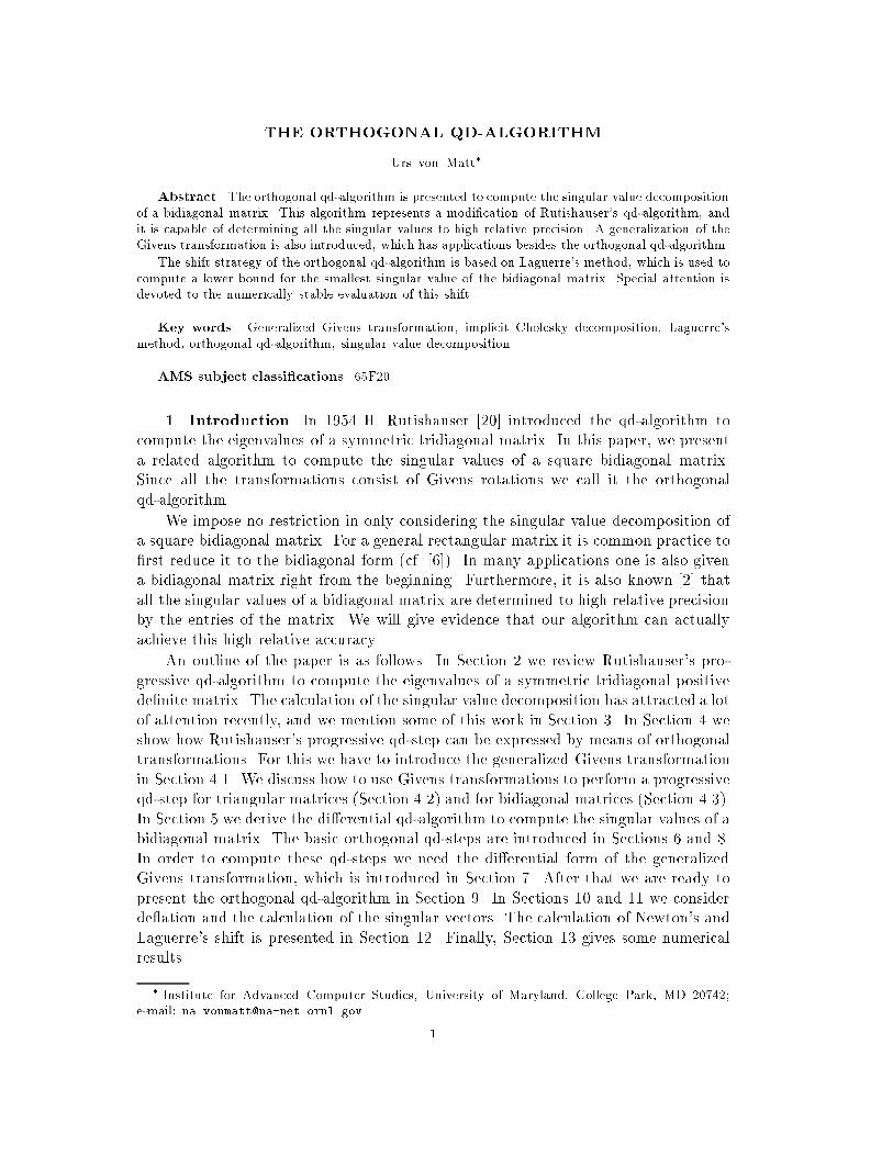
THE ORTHOGONAL QD-ALGORITHMUrs von Matt�Abstract. The orthogonal qd-algorithm is presented to compute the singular value decompositionof a bidiagonal matrix. This algorithm represents a modi�cation of Rutishauser's qd-algorithm, andit is capable of determining all the singular values to high relative precision. A generalization of theGivens transformation is also introduced, which has applications besides the orthogonal qd-algorithm.The shift strategy of the orthogonal qd-algorithm is based on Laguerre's method, which is used tocompute a lower bound for the smallest singular value of the bidiagonal matrix. Special attention isdevoted to the numerically stable evaluation of this shift.Key words. Generalized Givens transformation, implicit Cholesky decomposition, Laguerre'smethod, orthogonal qd-algorithm, singular value decomposition.AMS subject classi�cations. 65F20.1. Introduction. In 1954 H. Rutishauser [20] introduced the qd-algorithm tocompute the eigenvalues of a symmetric tridiagonal matrix. In this paper, we presenta related algorithm to compute the singular values of a square bidiagonal matrix.Since all the transformations consist of Givens rotations we call it the orthogonalqd-algorithm.We impose no restriction in only considering the singular value decomposition ofa square bidiagonal matrix. For a general rectangular matrix it is common practice to�rst reduce it to the bidiagonal form (cf. [6]). In many applications one is also givena bidiagonal matrix right from the beginning. Furthermore, it is also known [2] thatall the singular values of a bidiagonal matrix are determined to high relative precisionby the entries of the matrix. We will give evidence that our algorithm can actuallyachieve this high relative accuracy.An outline of the paper is as follows. In Section 2 we review Rutishauser's pro-gressive qd-algorithm to compute the eigenvalues of a symmetric tridiagonal positivede�nite matrix. The calculation of the singular value decomposition has attracted a lotof attention recently, and we mention some of this work in Section 3. In Section 4 weshow how Rutishauser's progressive qd-step can be expressed by means of orthogonaltransformations. For this we have to introduce the generalized Givens transformationin Section 4.1. We discuss how to use Givens transformations to perform a progressiveqd-step for triangular matrices (Section 4.2) and for bidiagonal matrices (Section 4.3).In Section 5 we derive the di�erential qd-algorithm to compute the singular values of abidiagonal matrix. The basic orthogonal qd-steps are introduced in Sections 6 and 8.In order to compute these qd-steps we need the di�erential form of the generalizedGivens transformation, which is introduced in Section 7. After that we are ready topresent the orthogonal qd-algorithm in Section 9. In Sections 10 and 11 we considerde ation and the calculation of the singular vectors. The calculation of Newton's andLaguerre's shift is presented in Section 12. Finally, Section 13 gives some numericalresults.� Institute for Advanced Computer Studies, University of Maryland, College Park, MD 20742;e-mail: na.vonmatt@na-net.ornl.gov. 1

2 Urs von MattSome important algorithms are presented in pseudo-code, and we choose a nota-tion corresponding to a modern procedural language of the Algol-family. This allowsus to concentrate on the mathematical properties of the algorithms, while an actualimplementation in any language can still be readily derived from our code.2. Rutishauser's Quotient-Di�erence Algorithm. Rutishauser used his qd-algorithm in order to compute the eigenvalues of a symmetric tridiagonal positivede�nite matrix A. He started with the Cholesky decompositionA = RTR;where R = 26666664 1 �1� � � � � �� � � �n�1 n 37777775is an n-by-n upper bidiagonal matrix. Afterwards, a sequence of so-called progressiveqd-steps is applied to the matrix R.Definition 2.1. A progressive qd-step with shift s transforms an n-by-n upperbidiagonal matrix R into another n-by-n upper bidiagonal matrix R0. It is de�ned bythe Cholesky decomposition RRT � sI = R0TR0:(1)This transformation is applicable if and only if s � �min(RTR).By a progressive qd-step the eigenvalues are shifted by the amount of s, i.e.�i(R0TR0) = �i(RTR)� s:All the eigenvalues of A can be computed by a proper shift strategy. Algorithm 1presents Rutishauser's progressive qd-algorithm in matrix terms (see also [5, p. 100]).The performance of the qd-algorithm depends critically on the choice of theshifts s. In [23] Rutishauser shows that, for s � 0, the matrices R converge to adiagonal matrix with the square roots of the eigenvalues of A. The convergence is lin-ear and becomes worse when the eigenvalues are clustered. Algorithm 1 is not suitedfor this shift strategy because, in general, its inner loop would not terminate.We can obtain a much better rate of convergence by choosing the shiftss = 1trace(RTR)�1 :In [24, pp. 484{486] it is shown how this shift can be computed easily from the ma-trix R. Reinsch and Bauer observe in [19] that this shift can be seen as a Newton stepfor the solution of the characteristic polynomialp(s) = det(RTR� sI):

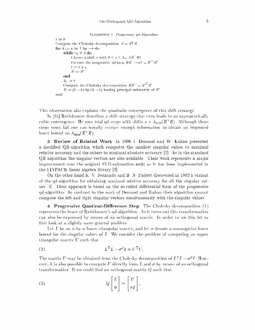
The Orthogonal QD-Algorithm 3Algorithm 1. Progressive qd-Algorithm.t := 0Compute the Cholesky decomposition A = RTR.for k := n to 1 by �1 dowhile k 6= 0 doChoose a shift s with 0 � s � �min(RTR).Execute the progressive qd-step RRT � sI = R0TR0.t := t+ sR := R0end�k := tCompute the Cholesky decomposition RRT = R0TR0.R := (k � 1)-by-(k � 1) leading principal submatrix of R0endThis observation also explains the quadratic convergence of this shift strategy.In [22] Rutishauser describes a shift strategy that even leads to an asymptoticallycubic convergence. He uses trial qd-steps with shifts s > �min(RTR). Although thesesteps must fail one can usually extract enough information to obtain an improvedlower bound on �min(RTR).3. Review of Related Work. In 1990 J. Demmel and W. Kahan presenteda modi�ed QR-algorithm which computes the smallest singular values to maximalrelative accuracy and the others to maximal absolute accuracy [2]. As in the standardQR-algorithm the singular vectors are also available. Their work represents a majorimprovement over the original SVD-subroutine svdc as it has been implemented inthe LINPACK linear algebra library [3].On the other hand K. V. Fernando and B. N. Parlett discovered in 1992 a variantof the qd-algorithm for obtaining maximal relative accuracy for all the singular val-ues [4]. Their approach is based on the so-called di�erential form of the progressiveqd-algorithm. In contrast to the work of Demmel and Kahan their algorithm cannotcompute the left and right singular vectors simultaneously with the singular values.4. Progressive Quotient-Di�erence Step. The Cholesky decomposition (1)represents the heart of Rutishauser's qd-algorithm. As it turns out this transformationcan also be expressed by means of an orthogonal matrix. In order to see this let us�rst look at a slightly more general problem.Let L be an n-by-n lower triangular matrix, and let � denote a nonnegative lowerbound for the singular values of L. We consider the problem of computing an uppertriangular matrix U such that LTL� �2I = UTU:(2)The matrix U may be obtained from the Cholesky decomposition of LTL� �2I . How-ever, it is also possible to compute U directly from L and � by means of an orthogonaltransformation. If we could �nd an orthogonal matrix Q such thatQ24L0 35 = 24 U�I 35 ;(3)

4 Urs von Matt2666666666664 ll11l21 l22��� ��� � � ���� ��� : : : � � �l0 � � � � � � 0 3777777777775 7�! 2666666666664 l�ll21 l22��� ��� � � ���� ��� : : : � � �� 0 � � � 0 3777777777775 7�! 2666666666664 � �0 ���� ��� � � ���� ��� : : : � � �� 0 � � � 0 3777777777775 7�!� � � 7�! 2666666666664 � � � � � �0 ���� ��� � � �0 � � � � �� 0 � � � 0 3777777777775 = 2666666666664 u vTL0� 0 � � � 0 3777777777775Fig. 1. Stage in the Implicit Cholesky Decomposition.we would have solved our problem, since (3) implies LTL = UTU + �2I , which isequivalent to (2). We call this approach the implicit Cholesky decomposition.We can obtain the decomposition (3) by a properly chosen sequence of Givenstransformations. In Figure 1 one stage of this decomposition is depicted which reducesthe dimension of the problem by one. By applying this step n times we can obtainthe desired decomposition (3).The nontrivial part of this stage consists in the �rst Givens transformation. In-stead of zeroing the entry l11, it introduces the value �. Obviously, we cannot usean ordinary Givens transformation for this purpose. Rather, we have to introduce ageneralization of the Givens transformation.4.1. Generalized Givens Transformation. Usually the Givens transforma-tion G := 24 c s�s c35(4)with c2 + s2 = 1 is determined such thatG24x1x2 35 = 24 r035 :The matrix G is therefore used to selectively annihilate elements in a vector or amatrix. But it is also possible to introduce another value � di�erent from zero:G24x1x2 35 = 24 r� 35 :(5)

The Orthogonal QD-Algorithm 5Algorithm 2. Generalized Givens Transformation (rotg2).scale := max(jx1j; jx2j)if scale = 0 thenc := 1s := 0else x1 := x1=scalex2 := x2=scalesig := �=scalenorm2 := x21 + x22r := pnorm2 � sig2c := (x1 � r + x2 � sig)=norm2s := (x2 � r � x1 � sig)=norm2x1 := scale � rx2 := �endThe value of r is given by r := �qx21 + x22 � �2:The choice of the sign is of no concern. One may opt for a positive r, or it may bemore useful to let r have the same sign as x1. Obviously, the transformation (5) isonly possible if j�j � qx21 + x22.We now demonstrate how to compute the quantities c and s in G. It is easilyveri�ed that 24 cs35 = 1x21 + x22 24x1 x2x2 �x1 3524 r� 35 :An implementation which avoids over ow is presented as Algorithm 2.We intend to present a detailed error analysis in a future paper. Let us justmention that the computed matrix G is orthogonal up to a small multiple of themachine precision, and the equation (5) is also satis�ed to high accuracy for thecomputed quantities.4.2. Implicit Cholesky Decomposition. So far, we have only described onestage of the implicit Cholesky decomposition in Figure 1. By applying this stepn times, we can compute the decomposition (3). This procedure is presented inpseudo-code as Algorithm 3. We describe the construction and application of or-dinary Givens rotations by calls of the BLAS routines rotg and rot. Their precisede�nition is given in [3, 11]. We also postulate the procedure rotg2 which calculatesa generalized Givens transformation according to Algorithm 2. More speci�cally, thecall rotg2 (x1, x2, �, c, s) determines the values of c and s such that equation (5)holds. The parameters x1 and x2 are overwritten by their transformed values. In thecase of �2 > x21 + x22 an error condition is raised.The following Theorem ensures that the generalized Givens transformation nec-essary in each stage will never fail.

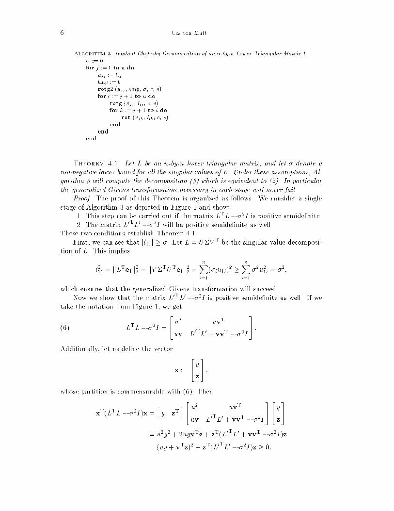
6 Urs von MattAlgorithm 3. Implicit Cholesky Decomposition of an n-by-n Lower Triangular Matrix L.U := 0for j := 1 to n doujj := ljjtmp := 0rotg2 (ujj, tmp, �, c, s)for i := j + 1 to n dorotg (ujj, lij , c, s)for k := j + 1 to i dorot (ujk, lik, c, s)endendendTheorem 4.1. Let L be an n-by-n lower triangular matrix, and let � denote anonnegative lower bound for all the singular values of L. Under these assumptions, Al-gorithm 3 will compute the decomposition (3) which is equivalent to (2). In particularthe generalized Givens transformation necessary in each stage will never fail.Proof. The proof of this Theorem is organized as follows. We consider a singlestage of Algorithm 3 as depicted in Figure 1 and show:1. This step can be carried out if the matrix LTL� �2I is positive semide�nite.2. The matrix L0TL0 � �2I will be positive semide�nite as well.These two conditions establish Theorem 4.1.First, we can see that jl11j � �. Let L = U�V T be the singular value decomposi-tion of L. This impliesl211 = kLTe1k22 = kV �TUTe1k22 = nXi=1(�iu1i)2 � nXi=1 �2u21i = �2;which ensures that the generalized Givens transformation will succeed.Now we show that the matrix L0TL0 � �2I is positive semide�nite as well. If wetake the notation from Figure 1, we getLTL� �2I = 24 u2 uvTuv L0TL0 + vvT � �2I 35 :(6)Additionally, let us de�ne the vector x := 24 yz35 ;whose partition is commensurable with (6). ThenxT(LTL� �2I)x = h y zT i24 u2 uvTuv L0TL0 + vvT � �2I 3524 yz35= u2y2 + 2uyvTz+ zT(L0TL0 + vvT � �2I)z= (uy + vTz)2 + zT(L0TL0 � �2I)z � 0:

The Orthogonal QD-Algorithm 7First we assume u 6= 0. In this case we can determine a y corresponding to each zsuch that uy + vTz = 0. This implieszT(L0TL0 � �2I)z � 0(7)for all z.Finally, assume that u = 0. As the orthogonal Givens transformations leave thenorm of the �rst column intact, we have�2 = nXi=1 l2i1 � l211 � �2:But this implies jl11j = � and li1 = 0 for i = 2; : : : ; n. Consequently, the ordinaryGivens transformations in this stage need not be carried out. The important pointhere is, that we have v = 0 in this special case. This implies uy + vTz = 0 too, andthe inequality (7) can be established for all z as well. But this observation proves theclaim that L0TL0 � �2I is a positive semide�nite matrix.Note that if the decomposition (3) exists, then from (2) it follows immediatelythat LTL � �2I is a positive semide�nite matrix. Therefore, the implicit Choleskydecomposition of a square lower triangular matrix L exists if and only if LTL � �2Iis a positive semide�nite matrix.There are a number of problems where the implicit Cholesky decomposition ex-hibits its advantages over its explicit counterpart. The explicit Cholesky decompo-sition is based on the factorization of the matrix A := LTL� �2I. The conditionnumber of A is at least the square of the condition number of L. This means thateven for a modestly ill-conditioned L the matrix A can become numerically singular.In this case the explicit Cholesky decomposition breaks down. Also, if A is close to asingular matrix the explicit Cholesky decomposition may loose accuracy. The readermay �nd a more detailed comparison in [26, pp. 47{53].4.3. Bidiagonal Matrices. In the special case of a progressive qd-step the ma-trix L has the shape of the n-by-n lower bidiagonal matrixL := 26666664�1�1 � � �� � � � � ��n�1 �n 37777775 :Due to the special structure of the matrix L we can use a simpli�ed version of thegeneral Algorithm 3. This is shown graphically in Figure 2 and as Algorithm 4. Notethat Algorithm 4 takes care of not overwriting the vectors � and �.5. Di�erential Quotient-Di�erence Algorithm. The evaluation of the Chol-esky decomposition (1) represents the heart of Rutishauser's qd-algorithm. As we havealready seen in Section 4.2 this factorization can also be obtained with the help of gen-eralized Givens transformations. Algorithm 4 gives us the decompositionQ24RT0 35 = 24 R0psI 35 ;

8 Urs von Matt2666666666664 l�1�1 �2�2 �3� � � � � �l0 0 0 � � � 3777777777775 7�! 2666666666664 l 01l�1 �2�2 �3� � � � � �� 0 0 � � � 3777777777775 7�! 2666666666664 1 �10 l~ 2�2 �3� � � � � �� l0 0 � � � 3777777777775 7�!2666666666664 1 �10 l 02l�2 �3� � � � � �� � 0 � � � 3777777777775 7�! 2666666666664 1 �10 2 �20 ~ 3� � � � � �� � 0 � � � 3777777777775 7�! � � �Fig. 2. Implicit Cholesky Decomposition of a Lower Bidiagonal Matrix L.Algorithm 4. Implicit Cholesky Decomposition of an n-by-n Lower Bidiagonal Matrix L. 1 := �1for k := 1 to n� 1 dotmp := 0rotg2 ( k, tmp, �, cos, sin)tmp := �krotg ( k, tmp, cos, sin)�k := 0 k+1 := �k+1rot (�k, k+1, cos, sin)endtmp := 0rotg2 ( n, tmp, �, cos, sin)which is equivalent to (1).It is now possible to modify the qd-Algorithm 1 to directly compute the singularvalues of an upper bidiagonal matrix R. We get Algorithm 5, which corresponds tothe di�erential qd-algorithm by Fernando and Parlett (cf. [4, Section 5]).This algorithm enables us to compute all the singular values of R to high relativeaccuracy (cf. [4, Section 7]). On the other hand, it is not suited to also compute thecorresponding singular vectors simultaneously with the singular values. The primaryreason for this is that the matrix R is transposed in each step. Consequently, it isnot possible to interpret Algorithm 5 as a sequence of orthogonal transformationsapplied from the left and the right to the matrix R, as it is the case with the ordinaryQR-algorithm (cf. [7, Section 8.3]).In order to remedy this de�ciency we will propose a new orthogonal qd-algorithm

The Orthogonal QD-Algorithm 9Algorithm 5. Di�erential qd-Algorithm.� := 0for k := n to 1 by �1 dowhile k 6= 0 doChoose a shift s with 0 � s � �min(R).Compute the implicit Cholesky decompositionQ �RT0 � = �R0sI � :� := p�2 + s2R := R0end�k := �Compute the QR-decomposition RT = QR0.R := (k � 1)-by-(k � 1) leading principal submatrix of R0endwhich transforms the (2n)-by-n matrixA := 24R0 35to a diagonal matrix with the help of orthogonal transformations applied from the leftand the right. So-called orthogonal qd-steps are the tool for doing this, and they willbe presented in the next sections.6. Orthogonal Quotient-Di�erence Steps I. LetL := 26666664�1�1 � � �� � � � � ��n�1 �n 37777775denote an n-by-n lower bidiagonal matrix, and letU := 26666664 1 �1� � � � � �� � � �n�1 n 37777775be an n-by-n upper bidiagonal matrix.Definition 6.1. Let Q be an orthogonal (2n)-by-(2n) matrix. We call the trans-formation Q24 L�I 35 = 24 Up�2 + s2I 35(8)

10 Urs von Matt2666666666664 l�1�1 �2�2 �3� � � � � �l� � � � � � 3777777777775 7�! 2666666666664 l 01l�1 �2�2 �3� � � � � �� � � � � � 3777777777775 7�! 2666666666664 1 �10 l~ 2�2 �3� � � � � �� l� � � � � 3777777777775 7�!2666666666664 1 �10 l 02l�2 �3� � � � � �� � � � � � 3777777777775 7�! 2666666666664 1 �10 2 �20 ~ 3� � � � � �� � � � � � 3777777777775 7�! � � �Fig. 3. Orthogonal Left lu-Step with Shift s.an orthogonal left lu-step with shift s.It follows from Theorem 4.1 that this transformation exists if and only if thecondition jsj � �min(L) holds. The singular values of L are diminished by the amountof the shift s, i.e. �2i (U) = �2i (L)� s2:The matrix Q can be constructed by the sequence of Givens rotations depicted in Fig-ure 3. The quantity � is an abbreviation for p�2 + s2. The use of generalized Givenstransformations may become problematic for small values of s, however. Assume, forinstance, that �1 and s are tiny, and � is so large that �2 + �21 = �2 numerically.In such a case, Algorithm 2 would transform �1 into 01 = 0 even if �21 � s2 > 0. Inorder to avoid this pitfall we introduce the di�erential form of the generalized Givenstransformation in the next section.7. Di�erential Form of the Generalized Givens Transformation. Thegeneralized Givens transformation, as it has been introduced in Section 4.1, is de-signed to introduce a given value into an element of a vector. Now, consider therelated problem of determining a Givens transformation (4) such thatG24x1x2 35 = 24 r1r2 35 ;(9)where r1 := sign(x1)qx21 � �2;(10) r2 := sign(x2)qx22 + �2:(11)

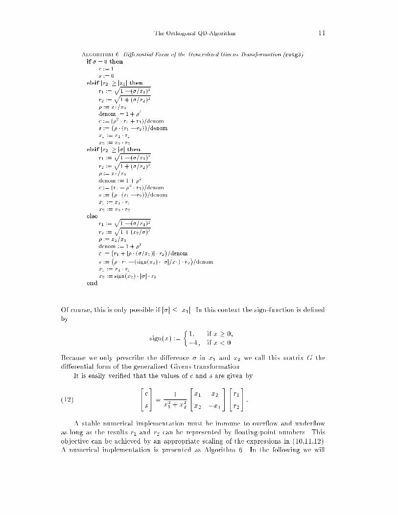
The Orthogonal QD-Algorithm 11Algorithm 6. Di�erential Form of the Generalized Givens Transformation (rotg3).if � = 0 thenc := 1s := 0elsif jx2j � jx1j thenr1 :=p1� (�=x1)2r2 :=p1 + (�=x2)2� := x1=x2denom := 1 + �2c := (�2 � r1 + r2)=denoms := �� � (r1 � r2)�=denomx1 := x1 � r1x2 := x2 � r2elsif jx2j � j�j thenr1 :=p1� (�=x1)2r2 :=p1 + (�=x2)2� := x2=x1denom := 1 + �2c := (r1 + �2 � r2)=denoms := �� � (r1 � r2)�=denomx1 := x1 � r1x2 := x2 � r2else r1 :=p1� (�=x1)2r2 :=p1 + (x2=�)2� := x2=x1denom := 1 + �2c := �r1 + j� � (�=x1)j � r2�=denoms := �� � r1 � (sign(x2) � j�j=x1) � r2�=denomx1 := x1 � r1x2 := sign(x2) � j�j � r2endOf course, this is only possible if j�j � jx1j. In this context the sign-function is de�nedby sign(x) := � 1; if x � 0,�1; if x < 0.Because we only prescribe the di�erence � in x1 and x2 we call this matrix G thedi�erential form of the generalized Givens transformation.It is easily veri�ed that the values of c and s are given by24 cs35 = 1x21 + x22 24x1 x2x2 �x1 3524 r1r2 35 :(12)A stable numerical implementation must be immune to over ow and under owas long as the results r1 and r2 can be represented by oating-point numbers. Thisobjective can be achieved by an appropriate scaling of the expressions in (10,11,12).A numerical implementation is presented as Algorithm 6. In the following we will

12 Urs von MattAlgorithm 7. Orthogonal Left lu-Step with Shift s. 1 := �1for k := 1 to n� 1 dotmp := �rotg3 ( k, tmp, s, cos, sin)tmp := �krotg ( k, tmp, cos, sin)�k := 0 k+1 := �k+1rot (�k, k+1, cos, sin)endtmp := �rotg3 ( n, tmp, s, cos, sin)abbreviate this computation by the subroutine call rotg3 (x1, x2, �, c, s) which over-writes the parameters x1 and x2 by their transformed values. The name rotg3 stemsfrom the BLAS subroutine rotg for the calculation of an ordinary Givens transforma-tion [3, 11]. It is erroneous to call rotg3 with j�j > jx1j.It is planned to give an error analysis in a future paper. We will show that thematrix G is orthogonal up to a small multiple of the machine precision. Furthermore,the key equation (9) always holds to high accuracy for the computed quantities.8. Orthogonal Quotient-Di�erence Steps II. An implementation of the or-thogonal left lu-step of Figure 3 is given by Algorithm 7.Definition 8.1. Let Q denote an orthogonal (2n)-by-(2n) matrix. We call thetransformation Q24 U�I 35 = 24 Lp�2 + s2I 35(13)an orthogonal left ul-step with shift s.This transformation represents the dual version of the orthogonal left lu-step. Itcan be carried out if and only if jsj � �min(U). The singular values of U are reducedby the amount of the shift s, i.e.�2i (L) = �2i (U)� s2:An orthogonal left ul-step, too, can be executed by a sequence of Givens rotations. Themechanism is the same as in Figure 3, with the only exception that the transformationsare applied from bottom to top.Definition 8.2. Let Q denote an orthogonal n-by-n matrix. We call the trans-formation 24 I QT 3524 U�I 35Q = 24 L�I 35(14)an orthogonal right ul-step.

The Orthogonal QD-Algorithm 132664 l 1 l�1 2 �2 3 � � �� � � 3775 7�! 2664 �1 0�1 l~�2 l�2 3 � � �� � � 3775 7�! 2664 �1 0�1 �2 0�2 ~�3 � � �� � � 3775 7�! � � �Fig. 4. Orthogonal Right ul-Step.Algorithm 8. Orthogonal Right ul-Step.�1 := 1for k := 1 to n� 1 dotmp := �krotg (�k, tmp, cos, sin)�k := 0�k+1 := k+1rot (�k, �k+1, cos, sin)endThis transformation can always be executed, and it leaves the singular values of Uunchanged. If n = 0 we have �n = �n�1 = 0 after the transformation. This propertywill be useful to de ate a matrix U with n = 0.The sequence of Givens rotations necessary for an orthogonal right ul-step isdepicted as Figure 4. The corresponding implementation is presented as Algorithm 8.Definition 8.3. Let Q denote an orthogonal n-by-n matrix. We call the trans-formation 24 I QT 3524 L�I 35Q = 24 U�I 35(15)an orthogonal right lu-step.This transformation represents the dual version of the orthogonal right ul-step.It can also be executed unconditionally, and it preserves the singular values of thematrix L. If the �rst row of L is zero, i.e. if �1 = 0, we get a matrix U with 1 = �1 = 0.We will therefore use this transformation to de ate a matrix L with �1 = 0.An orthogonal right lu-step can also be carried out by a sequence of Givens rota-tions. The same technique is used as shown in Figure 4, except that the transforma-tions are applied from bottom to top.We will refer to the four transformations, that have been introduced in this section,by the generic term of orthogonal qd-steps.Fernando and Parlett also present a root-free version of the orthogonal left lu-step in [4]. However, such a root-free algorithm has the disadvantage that it operateson the squares of the singular values. Consequently, the largest singular value mustnot exceed the square root of the largest machine-representable number. Similarly,singular values smaller than the square root of the smallest machine number under owto zero. We refrain from this version in order not to restrict the domain of calculationmore than necessary.

14 Urs von MattTable 1Choice of Orthogonal qd-Steps.Matrix Grading qd-Step Resultlower j�1j � j�nj left lu-step j 1j � j njbidiagonal j�1j < j�nj right lu-step j 1j < j njupper j 1j � j nj right ul-step j�1j � j�njbidiagonal j 1j < j nj left ul-step j�1j < j�njThe orthogonal qd-steps are closely related to the QR-algorithm for calculatingthe singular value decomposition (cf. [7, Section 8.3]). If we execute an orthogonal leftlu-step (8) with shift zero and an orthogonal right ul-step (14) in succession we getthe same result as by applying one unshifted QR-step. This has also been observedin [14, 15]. The same transformations are also useful for re�ning a URV-decomposition(see [14, 25] for more details).9. Orthogonal Quotient-Di�erence Algorithm. Now, we have available thefull set of orthogonal qd-steps to introduce the orthogonal qd-algorithm. We startfrom a given n-by-n lower bidiagonal matrix B whose singular value decomposition isdesired. The orthogonal qd-algorithm can be expressed as a sequence of left and rightqd-steps applied to the (2n)-by-n matrixA := 24B0 35 :The matrix A is transformed into the (2n)-by-n matrix24 0�35 ;where � denotes an n-by-n diagonal matrix with the singular values of B. In matrixterms this process can be described by the equation24B0 35 = P 24 0�35QT;(16)where P denotes an orthogonal (2n)-by-(2n) matrix, and Q denotes an orthogonaln-by-n matrix.In order to obtain rapid convergence the orthogonal qd-steps must preserve thegrading of the bidiagonal matrix (cf. [2, p. 891]). For instance, if we have a lowerbidiagonal matrix L with large entries in the top left corner and small entries in thelower right corner we will execute an orthogonal left lu-step. If the same matrix Lwere graded the opposite way we would choose an orthogonal right lu-step. In ourimplementation we only look at the �rst and last diagonal entry to determine thegrading of the matrix. We present all the four possible cases as Table 1. If, forinstance, we have a lower bidiagonal matrix L with j�1j � j�nj, we execute a leftlu-step and get an upper bidiagonal matrix U with j 1j � j nj.

The Orthogonal QD-Algorithm 1510. De ation. We would like to execute a de ation step as soon as an elementin the bidiagonal matrix L or U has become so small that it can be neglected. Thismeans that we can set this matrix entry to zero without changing the numericalsingular values of the matrix B in (16).Let us �rst analyse the situation when we set to zero a diagonal element �k in thematrix L. For this we compare the original matrixA := 24 L�I 35(17)with the modi�ed matrix ~A := 24 ~L�I 35 ;(18)where we obtain the matrix ~L := L� �kekeTk(19)from the matrix L by setting �k to zero. As an immediate consequence of the de�ni-tion (17) we get the equation�i(ATA) = �i(LTL) + �2 = �i(LLT) + �2:(20)By taking into account the de�nition (19) we can express the matrices LTL and LLTby LTL = ~LT ~L+ E1;(21) LLT = ~L~LT + E2;(22)where E1 := �2kekeTk + �k�k�1(ek�1eTk + ekeTk�1);E2 := �2kekeTk + �k�k(ekeTk+1 + ek+1eTk ):The Euclidean norms of the two perturbation matrices E1 and E2 are given bykE1k2 = 12 j�kj�j�kj+q�2k + 4�2k�1 � � j�kj�j�kj+ j�k�1j�;kE2k2 = 12 j�kj�j�kj+q�2k + 4�2k � � j�kj�j�kj+ j�kj�:As a consequence of Weyl's monotonicity theorem (cf. [18, pp. 191{194] and [27,pp. 101{103]) the norms of the perturbations E1 and E2 represent an upper bound forthe change of the eigenvalues in (21,22). More precisely, we can express the eigenvaluesof LTL and LLT by �i(LTL) = �i(~LT ~L) + uikE1k2;(23) �i(LLT) = �i(~L~LT) + vikE2k2;(24)

16 Urs von Mattwith juij � 1 and jvij � 1. If we substitute these results into equation (20), we get�2i (A) = �2i (~L) + �2 + uikE1k2 = �2i (~L) + �2 + vikE2k2:(25)We conclude that the singular values of A and ~A are equal to working precision, if theequation �2 +min(kE1k2; kE2k2) = �2applies numerically. Therefore, the condition�2 + j�kj�j�kj+min(j�k�1j; j�kj)� = �2(26)represents our numerical de ation criterion for neglecting a diagonal element �k. Itshould be noted that �0 = �n = 0. And, of course, the equivalent de ation criterionfor the upper bidiagonal matrix U is given by�2 + j kj�j kj+min(j�k�1j; j�kj)� = �2;(27)where �0 = �n = 0.Secondly, let us analyse the situation when an o�-diagonal element �k in L be-comes small. We also compare the two matrices A and ~A from (17,18) except that thematrix ~L is now given by ~L := L� �kek+1eTk :Equations (20,21,22) also apply for this case, and the perturbations E1 and E2 aregiven by E1 := �2kekeTk + �k+1�k(ek+1eTk + ekeTk+1);E2 := �2kek+1eTk+1 + �k�k(ekeTk+1 + ek+1eTk );with the normskE1k2 = 12 j�kj�j�kj+q�2k + 4�2k+1 � � j�kj�j�kj+ j�k+1j�;kE2k2 = 12 j�kj�j�kj+q�2k + 4�2k � � j�kj�j�kj+ j�kj�:The eigenvalue equations (23,24) as well as equation (25) still apply for the newperturbation matrices. Consequently, we are led to the numerical de ation criterion�2 + j�kj�j�kj+ min(j�kj; j�k+1j)� = �2(28)for neglecting an o�-diagonal element �k. The equivalent criterion for an upper bidi-agonal matrix U reads �2 + j�k j�j�kj+min(j kj; j k+1j)� = �2:(29)The de ation criterions (26,27,28,29) ensure the high relative accuracy of thecomputed singular values. If we also compute the left singular vectors additionalconditions need to be satis�ed. This issue is discussed in the next section.

The Orthogonal QD-Algorithm 1711. Singular Vectors. If we accumulate the orthogonal transformations in theorthogonal qd-algorithm we can compute the decomposition (16). In most cases,however, we would like to get the singular value decompositionB = U�V T(30)of the n-by-n lower bidiagonal matrix B, where U and V denote orthogonal n-by-n matrices. We will identify the matrix Q from (16) with the matrix V in (30). Onthe other hand we can recover the left singular vectors as a part of the matrix P . Inorder to see this we partition P into four n-by-n submatrices as follows:P = 24P11 P12P21 P22 35 :Then equation (16) is equivalent to24B0 35 = 24P11 P12P21 P22 3524 0�35QT:If � is nonsingular this implies P11 = P22 = 0, and P12 is an orthogonal matrix withthe left singular vectors. We will now show that we can get the same result in thepresence of rounding errors, even if B has small or zero singular values.Let us �rst analyse the e�ects of de ation. We assume that we have a lowerbidiagonal matrix L which satis�es the equation24B0 35 = P 24 L�I 35QT;where P and Q are orthogonal matrices. In order to express de ation in L we write Las L = L̂+�L;where L̂ denotes the de ated matrix, and �L is a rank-one matrix consisting of thematrix entry that has been removed from L. If we assume that all the calculationsafter the de ation are executed exactly we get the decomposition24B0 35 = P 24 L̂�I 35QT + P 24�L0 35QT = U 24 0�35V T + P 24�L0 35QT:Again U and V are orthogonal matrices. If we partition U and P into n-by-n subma-trices we get 24BV0 35 = 24U11 U12U21 U22 3524 0�35+ 24P11 P12P21 P22 3524�L0 35QTV:(31)

18 Urs von MattThis implies that 0 = U22�+ P21�LQTV:Note that all the singular values of � are greater than �. Consequently, we canwrite U22 as U22 = �P21�LQTV ��1;and the norm of U22 can be bounded bykU22k2 � k�Lk2� :We conclude that U11 and U22 are zero numerically if k�Lk2 � "�, where " denotesthe unit roundo� of the computer. This condition is met by the de ation criterionsj�k j � "�(32)and j�kj � "�:(33)The equivalent criterions for an upper bidiagonal matrix arej kj � "�(34)and j�kj � "�:(35)Note that the conditions (32,33,34,35) only ensure that the matrix U12 in (31) will benumerically orthogonal. We still need the conditions (26,27,28,29) to guarantee theaccuracy of the singular values.The de ation criterions (32,33,34,35) only work properly if � is su�ciently large.In particular, we require that � > m" ;where m denotes the under ow threshold. If B has some tiny or zero singular valuesthis condition will not be satis�ed right away. In this case we use zero-shift qd-stepsto determine the tiny singular values. We may expect these initial zero-shift qd-stepsto converge rapidly. Our implementation sets an o�-diagonal entry �k or �k to zero assoon as the de ation criterion 1 by Demmel and Kahan [2, p. 889] is met. Note thattwo zero-shift qd-steps are equivalent to one zero-shift QR iteration.

The Orthogonal QD-Algorithm 1912. Shifts. The performance of the orthogonal qd-algorithm mainly depends onthe choice of the shift s in each step. In this section we present two di�erent shiftstrategies based on Newton's and Laguerre's method to compute the zeros of a poly-nomial.Laguerre's method leads to a cubically convergent process. However, it is quiteexpensive to compute and it must also be carefully implemented to avoid numericalover ow problems. Unlike Wilkinson's shift, Laguerre's method will always computea lower bound for the smallest singular value of the bidiagonal matrix.In what follows we will compute Newton's and Laguerre's shift for an upper bidi-agonal matrix U . If we have to compute these shifts for a lower bidiagonal matrix L,we simply transpose it since this does not change the singular values.We may assume that U does not decouple, i.e. i 6= 0 and �i 6= 0. Otherwise wecould execute a de ation step and reduce the size of the problem.12.1. Newton's and Laguerre's Shift. The zeros of the characteristic poly-nomial p(�) := det(UTU � �I):are the eigenvalues of UTU , which are equal to the squares of the singular valuesof U . Thus if we use Newton's or Laguerre's method to approximate the smallest zeroof p(�) we can also get an approximation for the smallest singular value of U .Newton's method can be described by the iteration�k+1 = �k � r p(�k)p0(�k) ;and in the case of Laguerre's method we have�k+1 = �k � p(�k)p0(�k) n1�rn�rr �np0(�k)2�p(�k)p00(�k)p0(�k)2 � 1� :The value of r denotes the multiplicity of the zero that is being approached by theiteration (see also [8, 9, 10, 13, 16, 17] and [27, pp. 441{445]).If all the entries on the two diagonals of U are nonzero, then the eigenvaluesof UTU must be distinct [18, p. 124]. Consequently, p(�) has n distinct positive zeros,and we can always set r = 1. However, some of these zeros may lie so closely togetherthat they seem to be a multiple zero numerically. Unfortunately, the correspondingnumerical multiplicity r is usually not known a priori. This is another reason why wewill always set r = 1 in this section.We choose �0 = 0 as our initial value. It is well-known (cf. [8, 10, 16] and [27,pp. 443{445]) that both methods will then converge monotonically to the smallest zeroof p(�). In particular we have0 = �0 � �1 � �min(UTU):Laguerre's method enjoys cubic convergence provided that the multiplicity r is chosenproperly (cf. [16, pp. 353{362] and [27, pp. 443{445]). On the other hand Newton'smethod will converge only quadratically [27, p. 441].

20 Urs von MattWe intend to use p�1 as the shift in an orthogonal qd-step. Thus we de�neNewton's shift and Laguerre's shift as follows:sNewton := s�r p(0)p0(0) ;(36) sLaguerre := s� p(0)p0(0)vuuut n1 +rn�rr �np0(0)2�p(0)p00(0)p0(0)2 � 1� :(37)For r = 1, we can also view sLaguerre as an enlarged Newton step, and the second termin (37) serves as an acceleration factor for Newton's method.In the rest of this section we will be concerned with the numerically stable evalu-ation of these shifts. In [12] T. Y. Li and Z. Zeng discuss the same problem when theyevaluate Laguerre's shift for the symmetric tridiagonal eigenproblem. They avoid thecalculation of the characteristic polynomial p and its derivatives since these values arelikely to under ow or over ow. Fortunately, the key quantities in (36) and (37) aregiven by f := s� p(0)p0(0) = � nXk=1 1�2k��1=2 = �trace(UUT)�1��1=2;g := p0(0)2 � p(0)p00(0)p0(0)2 = nXk=1 1�4k� nXk=1 1�2k�2 = trace(UUT)�2�trace(UUT)�1�2 :It is easy to see that f and g can be bounded as follows:0 � f � �min(U);1n � g � 1:Obviously, both f and g are well-scaled and are not in danger of numerical over ow.However, the value of f may under ow if U has tiny singular values close to or smallerthan the under ow threshold. If this happens we choose s = 0 as our shift.The following lemma holds the key for the stable evaluation of f and g.Lemma 12.1. Let U be a nonsingular n-by-n upper bidiagonal matrix, and let Pand Q be orthogonal matrices such thatUPek = rkek;(38) PTUTQek = skek:(39)Then we have eTk (UUT)�1ek = 1r2k ;(40) eTk (UUT)�2ek = 1r2ks2k :(41)

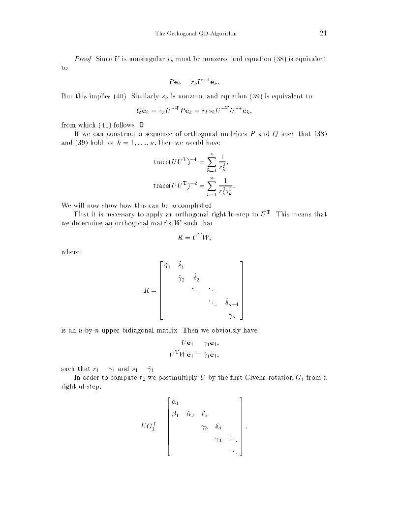
The Orthogonal QD-Algorithm 21Proof. Since U is nonsingular rk must be nonzero, and equation (38) is equivalentto Pek = rkU�1ek :But this implies (40). Similarly sk is nonzero, and equation (39) is equivalent toQek = skU�TPek = rkskU�TU�1ek;from which (41) follows.If we can construct a sequence of orthogonal matrices P and Q such that (38)and (39) hold for k = 1; : : : ; n, then we would havetrace(UUT)�1 = nXk=1 1r2k ;trace(UUT)�2 = nXk=1 1r2ks2k :We will now show how this can be accomplished.First it is necessary to apply an orthogonal right lu-step to UT. This means thatwe determine an orthogonal matrix W such thatR = UTW;where R = 26666666664 ~ 1 ~�1~ 2 ~�2� � � � � �� � � ~�n�1~ n 37777777775is an n-by-n upper bidiagonal matrix. Then we obviously haveUe1 = 1e1;UTWe1 = ~ 1e1;such that r1 = 1 and s1 = ~ 1.In order to compute r2 we postmultiply U by the �rst Givens rotation G1 from aright ul-step: UGT1 = 26666666664�1�1 ~�2 �2 3 �3 4 � � �� � � 37777777775 :

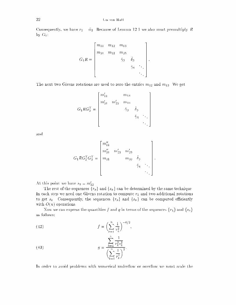
22 Urs von MattConsequently, we have r2 = ~�2. Because of Lemma 12.1 we also must premultiply Rby G1: G1R = 26666666664m11 m12 m13m21 m22 m23~ 3 ~�3~ 4 � � �� � � 37777777775 :The next two Givens rotations are used to zero the entries m12 and m13. We getG1RGT2 = 26666666664m011 m13m021 m022 m23~ 3 ~�3~ 4 � � �� � � 37777777775and G1RGT2GT3 = 26666666664m0011m0021 m022 m023m31 m33 ~�3~ 4 � � �� � � 37777777775 :At this point we have s2 = m022.The rest of the sequences frkg and fskg can be determined by the same technique.In each step we need one Givens rotation to compute rk and two additional rotationsto get sk . Consequently, the sequences frkg and fskg can be computed e�cientlywith O(n) operations.Now we can express the quantities f and g in terms of the sequences frkg and fskgas follows: f = � nXk=1 1r2k��1=2;(42) g = nXk=1 1r2ks2k� nXk=1 1r2k�2 :(43)In order to avoid problems with numerical under ow or over ow we must scale the

The Orthogonal QD-Algorithm 23expressions in (42) and (43). We propose the following two scaling factors:�k := mini�k jrij;�k := mini�k qjrijqjsij:We also introduce two sequences of scaled partial sums:�k := �2k kXi=1 1r2i ;�k := �4k kXi=1 1r2i s2i :It is important to note that we always have1 � �k � k;1 � �k � k:These two sequences can be evaluated recursively as follows:�1 = 1;�k = 8>>><>>>:� �k�k�1�2�k�1 + 1; if jrkj < �k�1,�k�1 + ��krk �2; if jrkj � �k�1,�1 = 1;�k = 8>>><>>>:� �k�k�1�4�k�1 + 1; if pjrkjpjskj < �k�1,�k�1 + � �kpjrkjpjskj�4; if pjrkjpjskj � �k�1.Now the values of f and g can be written asf = �np�n ;g = ��n�n�4 �n�2n ;and Newton's shift and Laguerre's shift are given bysNewton = f;sLaguerre = fvuuut n1 +r(n� 1)�ng � 1� :

24 Urs von MattTable 2Test Cases with Graded Matrices.Test Case n c �min �max1 50 2 8:325 � 10�1 6:450 � 10142 50 4 9:662 � 10�1 3:273 � 10293 50 0:5 2:189 � 10�16 1:467 � 1004 50 0:25 4:326 � 10�31 1:426 � 1005 100 2 8:325 � 10�1 7:262 � 10296 100 0:5 1:370 � 10�31 1:467 � 1007 500 1:1875 3:475 � 10�1 2:637 � 10378 500 0:875 2:510 � 10�31 1:672 � 10012.2. Bisection Shift. In theory an orthogonal qd-step with Newton's or La-guerre's shift s must always succeed since s is a lower bound for the singular values ofthe bidiagonal matrix. In oating point arithmetic, however, an orthogonal qd-stepmay occasionally fail due to rounding errors. The chance of failure increases as theshift s approaches the smallest singular value from below.If such a breakdown occurs we divide s by two and restart the orthogonal qd-step.We call this a bisection step. In unusual circumstances it may be necessary to repeatthis procedure several times.13. Numerical Results. We will now report on the numerical results obtainedfrom the orthogonal qd-algorithm. Our analysis is based on the performance of ourimplementation for two classes of test matrices, graded matrices and Toeplitz matrices.Let us �rst consider the class of graded matricesBgraded := 26666666666664 11 cc c2c2 � � �� � � cn�2cn�2 cn�1 37777777777775 ;which are also used as test matrices by Demmel and Kahan [2, Section 7] and byFernando and Parlett [4, Section 9.3]. The singular values �i of these matrices are of avastly di�erent size. The approximation �i � ci�1 gives a rough estimate of the orderof magnitude of �i.In Table 2 the di�erent values of n and c are summarized that we have used for ourtest matrices. We have run all the test cases in single precision on a DECstation 3100with a relative machine precision of " = 2�24 � 5:9605 � 10�8. The smallest positivenormalized number (under ow threshold) is given by m = 2�126 � 1:1755 � 10�38, andthe largest number (over ow threshold) is M = 2128(1� ") � 3:4028 � 1038.In Tables 3 and 4 we compare the orthogonal qd-algorithm with the subrou-tine sbdsqr from the LAPACK library [1]. This subroutine represents an implemen-tation of the work of Demmel and Kahan [2]. We have also used the procedure dbdsqr,which is an implementation of sbdsqr in double precision, to assess the accuracy of the

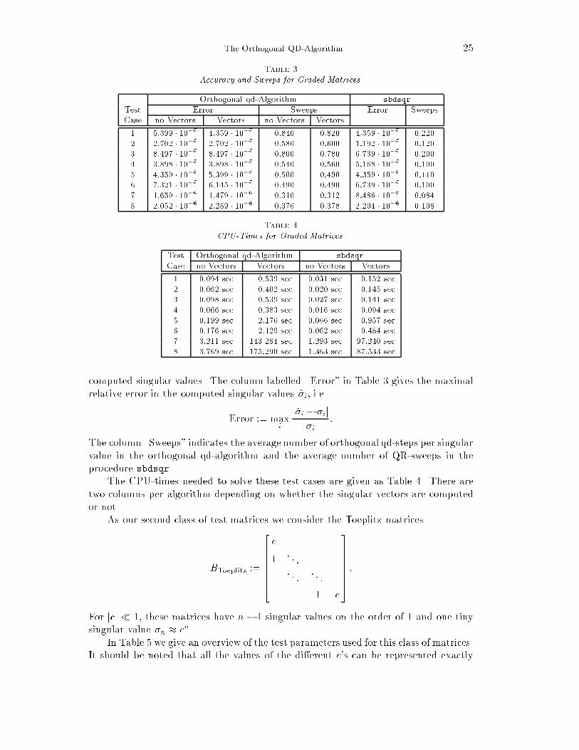
The Orthogonal QD-Algorithm 25Table 3Accuracy and Sweeps for Graded Matrices.Orthogonal qd-Algorithm sbdsqrTest Error Sweeps Error SweepsCase no Vectors Vectors no Vectors Vectors1 5:399 � 10�7 4:359 � 10�7 0:840 0:820 4:359 � 10�7 0:2202 2:702 � 10�7 2:702 � 10�7 0:580 0:600 1:192 � 10�7 0:1203 8:497 � 10�7 8:497 � 10�7 0:800 0:780 6:739 � 10�7 0:2004 3:898 � 10�7 3:898 � 10�7 0:540 0:560 5:168 � 10�7 0:1005 4:359 � 10�7 5:399 � 10�7 0:500 0:490 4:359 � 10�7 0:1106 7:321 � 10�7 6:145 � 10�7 0:490 0:490 6:739 � 10�7 0:1007 1:659 � 10�6 1:479 � 10�6 0:310 0:312 8:486 � 10�7 0:0848 2:052 � 10�6 2:289 � 10�6 0:376 0:378 2:204 � 10�6 0:108Table 4CPU-Times for Graded Matrices.Test Orthogonal qd-Algorithm sbdsqrCase no Vectors Vectors no Vectors Vectors1 0:094 sec 0:539 sec 0:031 sec 0:152 sec2 0:062 sec 0:402 sec 0:020 sec 0:145 sec3 0:098 sec 0:539 sec 0:027 sec 0:141 sec4 0:066 sec 0:383 sec 0:016 sec 0:094 sec5 0:199 sec 2:176 sec 0:066 sec 0:957 sec6 0:176 sec 2:129 sec 0:062 sec 0:484 sec7 3:211 sec 143:284 sec 1:293 sec 97:240 sec8 3:769 sec 175:290 sec 1:363 sec 87:533 seccomputed singular values. The column labelled \Error" in Table 3 gives the maximalrelative error in the computed singular values ~�i, i.e.Error := maxi j~�i � �ij�i :The column \Sweeps" indicates the average number of orthogonal qd-steps per singularvalue in the orthogonal qd-algorithm and the average number of QR-sweeps in theprocedure sbdsqr.The CPU-times needed to solve these test cases are given as Table 4. There aretwo columns per algorithm depending on whether the singular vectors are computedor not.As our second class of test matrices we consider the Toeplitz matricesBToeplitz := 26666664 c1 � � �� � � � � �1 c37777775 :For jcj � 1, these matrices have n � 1 singular values on the order of 1 and one tinysingular value �n � cn.In Table 5 we give an overview of the test parameters used for this class of matrices.It should be noted that all the values of the di�erent c's can be represented exactly

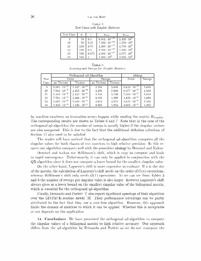
26 Urs von MattTable 5Test Cases with Toeplitz Matrices.Test Case n c �min �max9 50 0:5 6:661 � 10�16 1:499 � 10010 50 0:25 7:396 � 10�31 1:250 � 10011 100 0:75 1:403 � 10�13 1:750 � 10012 100 0:5 5:916 � 10�31 1:500 � 10013 500 0:875 2:366 � 10�30 1:875 � 10014 500 2 1:000 � 100 3:000 � 100Table 6Accuracy and Sweeps for Toeplitz Matrices.Orthogonal qd-Algorithm sbdsqrTest Error Sweeps Error SweepsCase no Vectors Vectors no Vectors Vectors9 5:061 � 10�7 1:337 � 10�6 4:160 5:640 8:620 � 10�7 1:66010 7:016 � 10�7 1:468 � 10�6 4:180 5:680 6:677 � 10�7 1:66011 1:333 � 10�6 2:425 � 10�6 4:140 5:790 7:303 � 10�7 1:61012 7:701 � 10�7 2:866 � 10�6 4:180 5:890 1:433 � 10�6 1:65013 4:007 � 10�6 1:039 � 10�5 4:042 5:574 4:625 � 10�6 1:44614 3:426 � 10�6 1:230 � 10�5 4:060 5:524 4:063 � 10�6 1:452by machine numbers; no truncation errors happen while reading the matrix BToeplitz.The corresponding results are shown as Tables 6 and 7. Note that in the case of theorthogonal qd-algorithm the number of sweeps is usually higher if the singular vectorsare also computed. This is due to the fact that the additional de ation criterions ofSection 11 also need to be satis�ed.The reader will have noticed that the orthogonal qd-algorithm computes all thesingular values for both classes of test matrices to high relative precision. In this re-spect our algorithm compares well with the procedure sbdsqr by Demmel and Kahan.Demmel and Kahan use Wilkinson's shift, which is easy to compute and leadsto rapid convergence. Unfortunately, it can only be applied in conjunction with theQR-algorithm since it does not compute a lower bound for the smallest singular value.On the other hand, Laguerre's shift is more expensive to evaluate. If n is the sizeof the matrix, the calculation of Laguerre's shift needs on the order of O(n) operations,whereas Wilkinson's shift only needs O(1) operations. As we can see from Tables 3and 6 the number of sweeps per singular value is also larger. However Laguerre's shiftalways gives us a lower bound on the smallest singular value of the bidiagonal matrix,which is essential for the orthogonal qd-algorithm.Finally, Fernando and Parlett [4] also report signi�cant speedups of their algorithmover the LINPACK-routine dsvdc [3]. Their performance advantage can be partlyattributed to the fact that they use a root-free algorithm. However, this approachlimits the domain of matrices to which it can be applied. Whether this is acceptableor not depends on the application.14. Conclusions. We have presented the orthogonal qd-algorithm to computethe singular values of a bidiagonal matrix to high relative accuracy. Our approachdi�ers from the qd-algorithm by Fernando and Parlett as we do not transpose the

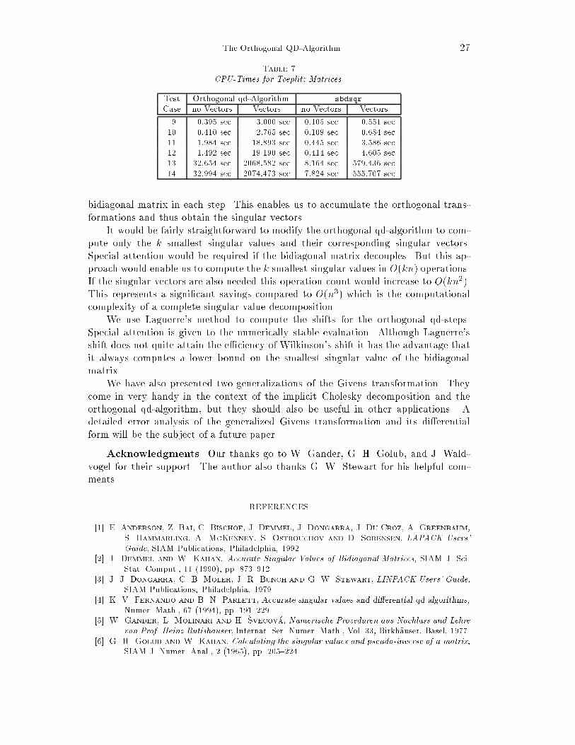
The Orthogonal QD-Algorithm 27Table 7CPU-Times for Toeplitz Matrices.Test Orthogonal qd-Algorithm sbdsqrCase no Vectors Vectors no Vectors Vectors9 0:395 sec 3:000 sec 0:105 sec 0:551 sec10 0:410 sec 2:765 sec 0:109 sec 0:684 sec11 1:984 sec 18:893 sec 0:445 sec 3:586 sec12 1:492 sec 19:190 sec 0:414 sec 4:605 sec13 32:654 sec 2068:582 sec 8:164 sec 579:436 sec14 32:994 sec 2074:473 sec 7:824 sec 555:707 secbidiagonal matrix in each step. This enables us to accumulate the orthogonal trans-formations and thus obtain the singular vectors.It would be fairly straightforward to modify the orthogonal qd-algorithm to com-pute only the k smallest singular values and their corresponding singular vectors.Special attention would be required if the bidiagonal matrix decouples. But this ap-proach would enable us to compute the k smallest singular values in O(kn) operations.If the singular vectors are also needed this operation count would increase to O(kn2).This represents a signi�cant savings compared to O(n3) which is the computationalcomplexity of a complete singular value decomposition.We use Laguerre's method to compute the shifts for the orthogonal qd-steps.Special attention is given to the numerically stable evaluation. Although Laguerre'sshift does not quite attain the e�ciency of Wilkinson's shift it has the advantage thatit always computes a lower bound on the smallest singular value of the bidiagonalmatrix.We have also presented two generalizations of the Givens transformation. Theycome in very handy in the context of the implicit Cholesky decomposition and theorthogonal qd-algorithm, but they should also be useful in other applications. Adetailed error analysis of the generalized Givens transformation and its di�erentialform will be the subject of a future paper.Acknowledgments. Our thanks go to W. Gander, G. H. Golub, and J. Wald-vogel for their support. The author also thanks G. W. Stewart for his helpful com-ments. REFERENCES[1] E. Anderson, Z. Bai, C. Bischof, J. Demmel, J. Dongarra, J. Du Croz, A. Greenbaum,S. Hammarling, A. McKenney, S. Ostrouchov and D. Sorensen, LAPACK Users'Guide, SIAM Publications, Philadelphia, 1992.[2] J. Demmel and W. Kahan, Accurate Singular Values of Bidiagonal Matrices, SIAM J. Sci.Stat. Comput., 11 (1990), pp. 873{912.[3] J. J. Dongarra, C. B. Moler, J. R. Bunch and G. W. Stewart, LINPACK Users' Guide,SIAM Publications, Philadelphia, 1979.[4] K. V. Fernando and B. N. Parlett, Accurate singular values and di�erential qd algorithms,Numer. Math., 67 (1994), pp. 191{229.[5] W. Gander, L. Molinari and H. �Svecov�a, Numerische Prozeduren aus Nachlass und Lehrevon Prof. Heinz Rutishauser, Internat. Ser. Numer. Math., Vol. 33, Birkh�auser, Basel, 1977.[6] G. H. Golub and W. Kahan, Calculating the singular values and pseudo-inverse of a matrix,SIAM J. Numer. Anal., 2 (1965), pp. 205{224.

28 Urs von Matt[7] G. H. Golub and C. F. Van Loan,Matrix Computations, Second Edition, The Johns HopkinsUniversity Press, Baltimore, 1989.[8] E. Hansen and M. Patrick, A Family of Root Finding Methods, Numer. Math., 27 (1977),pp. 257{269.[9] W. Kahan, Where does Laguerre's method come from?, in Proceedings of the Fourth AnnualPrinceton Conference on Information Sciences and Systems, Department of Electrical Engi-neering, Princeton University, Princeton, 1970, p. 143.[10] W. Kahan, Notes on Laguerre's Iteration, unpublished manuscript, Berkeley, 1992.[11] C. L. Lawson, R. J. Hanson, D. R. Kincaid and F. T. Krogh, Basic Linear AlgebraSubprograms for Fortran Usage, ACM Trans. Math. Softw., 5 (1979), pp. 308{325.[12] T. Y. Li and Z. Zeng, The Laguerre iteration in solving the symmetric tridiagonal eigenprob-lem, revisited, SIAM J. Sci. Comput., 15 (1994), pp. 1145{1173.[13] H. J. Maehly, Zur iterativen Au �osung algebraischer Gleichungen, ZAMP, 5 (1954), pp. 260{263.[14] R. Mathias and G. W. Stewart, A Block QR Algorithm and the Singular Value Decomposi-tion, Linear Algebra Appl., 182 (1993), pp. 91{100.[15] M. Moonen, P. Van Dooren and F. Vanpoucke, On the QR Algorithm and Updating theSVD and the URV Decomposition in Parallel, Linear Algebra Appl., 188/189 (1993), pp. 549{568.[16] A. M. Ostrowski, Solution of Equations in Euclidean and Banach Spaces, Third Edition of\Solution of Equations and Systems of Equations", Academic Press, New York, 1973.[17] B. N. Parlett, Laguerre's Method Applied to the Matrix Eigenvalue Problem, Math. Comp.,18 (1964), pp. 464{485.[18] B. N. Parlett, The Symmetric Eigenvalue Problem, Prentice-Hall, Englewood Cli�s, 1980.[19] C. H. Reinsch and F. L. Bauer, Rational QR Transformation with Newton Shift for SymmetricTridiagonal Matrices, Numer. Math., 11 (1968), pp. 264{272.[20] H. Rutishauser, Der Quotienten-Di�erenzen-Algorithmus, ZAMP, 5 (1954), pp. 233{251.[21] H. Rutishauser, Der Quotienten-Di�erenzen-Algorithmus, Mitteilungen aus dem Institut f�urangewandte Mathematik Nr. 7, Birkh�auser, Basel, 1957.[22] H. Rutishauser, �Uber eine kubisch konvergente Variante der LR-Transformation, ZAMM,40 (1960), pp. 49{54.[23] H. Rutishauser, Les propri�et�es num�eriques de l'algorithme quotient-di��erence, RapportEUR 4083f, Communaut�e Europ�eenne de l'Energie Atomique - EURATOM, Luxembourg,1968.[24] H. Rutishauser, Lectures on Numerical Mathematics, Birkh�auser, Boston, 1990.[25] G. W. Stewart, An Updating Algorithm for Subspace Tracking, IEEE Trans. Signal Processing,40 (1992), pp. 1535{1541.[26] U. von Matt, Large Constrained Quadratic Problems, Verlag der Fachvereine, Z�urich, 1993.[27] J. H. Wilkinson, The Algebraic Eigenvalue Problem, Clarendon Press, Oxford, 1965.