Università degli Studi di Bologna

DEIS

Biometric System Laboratory

Incremental Learning by Message Passing

in Hierarchical Temporal Memory

Davide Maltoni

Biometric System Laboratory

DEIS - University of Bologna (Italy)

davide.maltoni@unibo.it

Erik M. Rehn

Bernstein Center for Computational

Neuroscience Berlin

erik.m.rehn@gmail.com

May, 2012

DEIS Technical Report

1

Incremental Learning by Message Passing

in Hierarchical Temporal Memory

Davide Maltoni and Erik M. Rehn

Abstract — Hierarchical Temporal Memory (HTM) is a biologically-inspired framework that can be used to learn invariant rep-

resentations of patterns in a wide range of applications. Classical HTM learning is mainly unsupervised and once training is completed

the network structure is frozen, thus making further training (i.e. incremental learning) quite critical. In this paper we develop a novel

technique for HTM (incremental) supervised learning based on error minimization. We prove that error backpropagation can be nat-

urally and elegantly implemented through native HTM message passing based on Belief Propagation. Our experimental results show

that a two stage training composed by unsupervised pre-training + supervised refinement is very effective (both accurate and efficient).

This is in line with recent findings on other deep architectures.

1. INTRODUCTION

Hierarchical Temporal memory (HTM) is a biologically-inspired pattern recognition framework fairly unknown

to the research community [1]. It can be conveniently framed into Multi-stage Hubel-Wiesel Architectures [2] which

is a specific subfamily of Deep Architectures [3-5]. HTM tries to mimic the feed-forward and feedback projections

thought to be crucial for cortical computation. Bayesian Belief Propagation is used in a hierarchical network to learn

invariant spatio-temporal features of the input data and theories exist to explain how this mathematical model could

be mapped onto the cortical-thalamic anatomy [7-8].

A comprehensive description of HTM architecture and learning algorithms is provided in [6], where HTM was al-

so proved to perform well on some pattern recognition tasks, even though further studies and validations are neces-

sary. In [6] HTM is compared with MLP (Multiplayer Perceptron) and CN (Convolutional Network) on some pattern

recognition problems.

One limitation of the classical HTM learning is that once a network is trained it is hard to learn from new patterns

without retraining it from scratch. In other words a classical HTM is well suited for a batch training based on a fixed

training set, and it cannot be effectively trained incrementally over new patterns that were initially unavailable. In

fact, every HTM level has to be trained individually and in sequence, starting from the bottom: altering the internal

node structure at one network level (e.g. coincidences, groups) would invalidate the results of the training at higher

levels. In principle, incremental learning could be carried out in a classical HTM by updating only the output level,

but this is a naive strategy that works in practice only if the new incoming patterns are very similar to the existing

ones in terms of "building blocks". Since incremental training is a highly desirable property of a learning system, we

were motivated to investigate how HTM framework could be extended in this direction.

In this paper we present a two-stage training approach, unsupervised pre-training + supervised refinement, that

can be used for incremental learning: a new HTM is initially pre-trained (batch), then its internal structure is incre-

2

mentally updated as new labeled samples become available. This kind of unsupervised pre-training and supervised

refinement was recently demonstrated to be successful for other deep architectures [3].

The basic idea of our approach is to perform the batch pre-training using the algorithms described in [6] and then

fix coincidences and groups throughout the whole network; then, during supervised refinement we adapt the elements

of the probability matrices (for the output node) and (for the intermediate nodes) as if they were the

weights of a MLP neural network trained with backpropagation. To this purpose we first derived the update rules

based on the descent of the error function. Since the HTM architecture is more complex than MLP the resulting equa-

tions are not simple; further complications arise from the fact that and values are probabilities and need to

be normalized after each update step. Fortunately we found a surprisingly simple (and computationally light) way to

implement the whole process through native HTM message passing.

Our initial experiments show very promising results. Furthermore, the proposed two-stage approach not only ena-

bles incremental learning, but is also helpful for keeping the network complexity under control, thus improving the

framework scalability.

2. BACKGROUND

An HTM has a hierarchical tree structure. The tree is built up by levels (or layers), each composed of one

or more nodes. A node in one level is bidirectionally connected to one or more nodes in the level above and the num-

ber of nodes in each level decreases as we ascend the hierarchy. The lowest level, , is the input level and the high-

est level, , with typically only one node, is the output level. Levels and nodes in between input and output

are called intermediate levels and nodes. When an HTM is used for visual inference, as is the case in this study, the

input level typically has a retinotopic mapping of the input. Each input node is connected to one pixel of the input

image and spatially close pixels are connected to spatially close nodes. Figure 1 shows a graphical representation of a

simple HTM, its levels and nodes.

It is possible, and in many cases desirable, for a HTM to have an architecture where every intermediate node has

multiple parents. This creates a network where nodes have overlapping receptive fields. Throughout this paper a non-

overlapping architecture is used instead, where nodes only have one parent, to reduce computational complexity.

2.1 INFORMATION FLOW

In an HTM the flow of information is bidirectional. Belief propagation is used to pass message both up (feed-

forward) and down (feedback) the hierarchy as new evidence is presented to the network. The notation used here for

belief propagation (see Figure 2) closely follows Pearl [9] and is adapted to HTMs by George [10]:

Evidence coming from below is denoted . In visual inference this is an image or video frame presented to level

of the network.

Evidence from the top is denoted and can be viewed as contextual information. This can for instance be input

from another sensor modality or the absolute knowledge given by the supervisor training the network.

3

Fig. 1. A four-level HTM designed to work with 16x16 pixel images. Level 0 has 16x16 input nodes, each associated to a single

pixel. Each level 1 node has 16 child nodes (arranged in a 4×4 region) and a receptive field of 16 pixels. Each level 2 node has 4

child nodes (2×2 region) and a receptive field of 64 pixels. Finally, the single output node at level 3 has 4 child nodes (2×2 re-

gion) and a receptive field of 256 pixels.

Feed-forward messages passed up the hierarchy are denoted and feedback messages flowing down are denoted

.

Messages entering and leaving a node from below are denoted and respectively, relative to that node. Fol-

lowing the same notation as for the evidence, messages entering and leaving a node from above are denoted

and .

Fig. 2. Notation for message passing between HTM nodes.

Level 3

(output)

1 node

Level 2 (in-

termediate)

2×2 nodes

Level 1 (in-

termediate)

4×4 nodes

Level 0 (in-

put)

16×16 nodes

Image

16×16 pixels

4

When the purpose of an HTM is that of a classifier, the feed-forward message of the output node is the posterior

probability that the input belongs to one of the problem classes. We denoted this posterior as , where

is one of classes.

2.2 INTERNAL NODE STRUCTURE AND PRE-TRAINING

HTM training is performed level by level, starting from the first intermediate level. The input level does not need

any training it just forwards the input. Intermediate levels training is unsupervised and the output level training is

supervised. For a detailed description, including algorithm pseudocode, the reader should refer to [6].

For every intermediate node (Figure 3), a set of so called coincidence-patterns (or just coincidences) and a

set, , of coincidence groups, have to be learned. A coincidence, , is a vector representing a prototypical activation

pattern of the node’s children. For a node in , with input nodes as children, this corresponds to an image patch of

the same size as the node’s receptive field. For nodes higher up in the hierarchy, with intermediate nodes as children,

each element of a coincidence, , is the index of a coincidence group in child . Coincidence groups, also called

temporal groups, are clusters of coincidences likely to originate from simple variations of the same input pattern.

Coincidences found in the same group can be spatially dissimilar but likely to be found close in time when a pattern

is smoothly moved through the node’s receptive field. By clustering coincidences in this way, exploiting the temporal

smoothness of the input, invariant representations of the input space can be learned [10]. The assignment of coinci-

dences to groups within each node is encoded in a probability matrix ; each element repre-

sents the likelihood that a group, , is activated given a coincidence . These probability values are the elements we

will manipulate to incrementally train a network whose coincidences and groups have previously been learned and

fixed.

Fig. 3. Graphical representation of the information processing within an intermediate node. The two central boxes, and ,

constitutes the node memory at the end of training.

5

The structure and training of the output node differs from that of the intermediate nodes. In particular the output

node does not have groups but only coincidences. Instead of memorizing groups and group likelihoods it stores a

probability matrix , whose elements represents the likelihood of class given the coinci-

dence . This is learned in a supervised fashion by counting how many times every coincidence is the most active

one (“the winner”) in the context of each class. The output node also keeps a vector of class priors, , used to

calculate the final class posterior.

2.3 FEED-FORWARD MESSAGE PASSING

Inference in an HTM in conducted through feed-forward belief propagation (see [6]). When a node receives a set

of messages from its children,

, a degree of certainty over each of the coincidence in the

node is computed. This quantity is represented by a vector and can be seen as the activation of the node coinci-

dences. The degree of certainty over coincidence is

(1)

where is a normalization constant, and σ is a parameter controlling how quickly the activation level decays when

deviates from .

If the node is an intermediate node, it then computes its feed-forward message which is a vector of length and

is proportional to where is the set of all coincidence groups in the node and the cardinality of . Each

component of is

(2)

where is the number of coincidences stored in the node.

The feed-forward message from the output node, the network output, is the posterior class probability and is com-

puted in the following way:

(3)

where is a normalization constant such that .

2.4 FEEDBACK MESSAGE PASSING

The top-down information flow is used to give contextual information about the observed evidence. Each inter-

mediate node fuses top-down and bottom-up information to consolidate a posterior belief in its coincidence-patterns

[10]. Given a message from the parent, , the top-down activation of each coincidence, , is

6

(4)

The belief in coincidence is then given by:

(5)

The message sent by an intermediate node (belonging to a level ) to its the children, , is computed using

this belief distribution. The component of the message to a specific child node is

(6)

where

is the indicator function defined as

(7)

The top-down message sent from the output node is computed in a similar way:

(8)

Equation 6 and 8 will be important when we, in the next Section, show how to incrementally update the

and matrices to produce better estimates of the class posterior given some evidence from above.

3. HTM SUPERVISED REFINEMENT

This Section introduces a novel way to optimize an already trained HTM. The algorithm, called HSR (Htm Su-

pervised Refinement) shares many features with traditional backpropagation used to train multilayer perceptrons and

is inspired by weight fine-tuning methods applied to other deep belief architectures [3]. It exploits the belief propaga-

tion equations presented above to propagate an error message from the output node back through the network. This

enables each node to locally update its internal probability matrix in a way that minimizes the difference between the

estimated class posterior of the network and the posterior given from above, by a supervisor.

Our goal is to minimize the expected quadratic difference between the network output posterior given the evi-

dence from below, , and the posterior given the evidence from above, . To this purpose we employ empirical

risk minimization [11] resulting in the following loss function:

(9)

7

where is the number of classes, is the class posterior given the evidence from above, and

is

the posterior produced by the network using the input as evidence (i.e., inference). The loss function is also a func-

tion of all network parameters involved in the inference process. In most cases is a supervisor with absolute

knowledge about the true class , thus .

To minimize the empirical risk we first find the direction in which to alter the node probability matrices to de-

crease the loss and then apply gradient descent.

3.1 OUTPUT NODE UPDATE

For the output node which does not memorize coincidence groups, we update probability values stored in

the matrix, through the gradient descent rule:

(10)

where is the learning rate. The negative gradient of the loss function is given by:

which can be shown (see Appendix A for a derivation) to be equivalent to:

(11)

(12)

where

. We call the error message for class given some top-down

and bottom-up evidence.

3.2 INTERMEDIATE NODES UPDATE

For each intermediate node we update probability values in the matrix, through the gradient descent rule:

(13)

For intermediate nodes at level (i.e., the last but the output level) it can be shown (Appendix B) that:

(14)

8

where is the child portion of the message

sent from the output node to its children, but with replacing

the posterior (compare Eq. 15 with Eq. 8):

(15)

Finally, it can be shown that this generalizes to all levels of an HTM, and that all intermediate nodes can be updated

using messages from their immediate parent. The derivation can be found in Appendix C. In particular, the error

message from an intermediate node (belonging to a level ) to its child nodes is given by:

(16)

These results allow us to define an efficient and elegant way to adapt the probabilities in an already trained HTM

using belief propagation equations.

3.3 HSR PSEUDOCODE

A batch version of HSR algorithm is here provided:

HSR( ) {

for each training example in {

Present the example to the network and perform inference (eqs. 1,2 and 3)

Accumulate

values for the output node (eqs. 11 and 12)

Compute the error message (eq. 15)

for each child of the output node:

call BackPropagate(child, ) (see function below)

}

Update by using accumulated

(eq. 10)

Renormalize such that for each class ,

for each intermediate node

{ Update by using accumulated

(eq. 13)

Renormalize such that for each group ,

}

}

function BackPropagate(node, )

{

Accumulate

values for the node (eq. 14)

if (node level > 1)

{ Compute the error message (eq. 16)

for each child of node:

call BackPropagate(child, )

}

}

9

By updating the probability matrices for every training example, instead of at the end of the presentation of a group

of patterns, an online version of the algorithm is obtained. Both batch and online versions of HSR are investigated in

the experimental section.

In many cases it is preferable for the nodes in lower intermediate levels to share memory, so called node sharing

[6]. This speeds up training and forces all the nodes of the level to respond in the same way when the same stimulus

is presented at different places in the receptive field. In a level operating in node sharing, update (eq. 13) must

be performed only for the master node.

4. EXPERIMENTS

To verify the efficacy of the HSR algorithm we designed a number of experiments. These are performed using the

SDIGIT dataset which is a machine generated digit recognition problem [6]. SDIGIT patterns (16×16 pixels,

grayscale images) are generated by geometric transformations of class prototypes called primary patterns. The possi-

bility of randomly generating new patterns makes this dataset suitable for evaluating incremental learning algorithms.

By varying the amount of scaling and rotation applied to the primary patterns we can also control the problem diffi-

culty.

With we denote a set of patterns, including, for each of the 10

digits, the primary pattern and further patterns generated by simultaneous scaling and rotation of the

primary pattern according to random triplets where , and

. The creation of a test set starts by translating each of

the 10 primary pattern at all positions that allow it to be fully contained (with a 2 pixel background offset) in the

16×16 window thus obtaining patterns; then, for each of the patterns, further patterns are generated

by transforming the pattern according to random triplets ; the total number of patterns in the test set is then

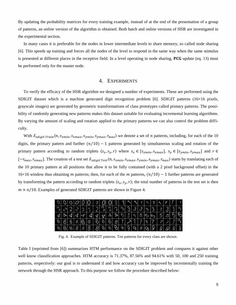
. Examples of generated SDIGIT patterns are shown in Figure 4.

Fig. 4. Example of SDIGIT patterns. Ten patterns for every class are shown.

Table I (reprinted from [6]) summarizes HTM performance on the SDIGIT problem and compares it against other

well know classification approaches. HTM accuracy is 71.37%, 87.56% and 94.61% with 50, 100 and 250 training

patterns, respectively: our goal is to understand if and how accuracy can be improved by incrementally training the

network through the HSR approach. To this purpose we follow the procedure described below:

10

SDIGIT - test set: (6,200 patterns, 10 classes)

Training set Approach Accuracy (%) Time (hh:mm:ss) Size

(MB) Train test train test

<50,0.70,1.0,0.7,1.0,40°>

1788 translated patterns

NN 100 57.92 < 1 sec 00:00:04 3.50

MLP 100 61.15 00:12:42 00:00:03 1.90

LeNet5 100 67.28 00:07:13 00:00:11 0.39

HTM 100 71.37 00:00:08 00:00:13 0.58

<100,0.70,1.0,0.7,1.0,40°>

3423 translated patterns

NN 100 73.63 < 1 sec 00:00:07 6.84

MLP 100 75.37 00:34:22 00:00:03 1.90

LeNet5 100 79.31 00:10:05 00:00:11 0.39

HTM 100 87.56 00:00:25 00:00:23 1.00

<250,0.70,1.0,0.7,1.0,40°>

8705 translated patterns

NN 100 86.50 < 1 sec 00:00:20 17.0

MLP 99.93 86.08 00:37:32 00:00:03 1.90

LeNet5 100 89.17 00:14:37 00:00:11 0.39

HTM 100 94.61 00:02:04 00:00:55 2.06

Table I. HTM compared against other techniques on SDIGIT problem (the table is reprinted from [6]). Three experiments are

performed with an increasing number of training patterns: 50, 100 and 250. The test set is common across the experiments and

include 6,200 patterns. NN, MLP and LeNet5 refer to Nearest Neighbor, Multi-Layer Perceptron and Convolutional Network,

respectively. HTM refers to a four-level Hierarchical Temporal Memory (whose architecture is shown in Figure 1) trained in

MaxStab configuration with Fuzzy grouping enabled.

Generate a pre-training dataset

Pre-train a new HTM on (training algs and params are as in [6], leading to Table I results)

for each epoch {

Generate a dataset (6,200 patterns)

Test HTM on for each iteration

call HSR( )

}

Test HTM on

In our experimental procedure we first pre-train a new network using a dataset (with patterns) and then for a

number of epochs we generate new datasets and apply HSR. At each epoch one can apply HSR for more iterations,

to favor convergence. However, we experimentally found that a good trade-off between convergence time and

overfitting can be achieved by performing just two HSR iterations for each epoch. The classification accuracy is cal-

culated using the patterns generated for every epoch but before the network is updated using those patterns. In this

way we emulate a situation where the network is trained on sequentially arriving patterns.

4.1 TRAINING CONFIGURATIONS

We assessed the efficacy of the HSR algorithm for different configurations:

batch vs online updating: see Section 3.3;

error vs all selection strategy: in error selection strategy, supervised refinement is performed only for patterns

that were misclassified by the current HTM, while in all selection strategy is performed over all patterns;

11

learning rate : see Equations 10 and 13. One striking find of our experiments is that the learning rate for the out-

put node should be kept much lower than for the intermediate nodes. In the following we refer to the learning rate

for output node as and to the learning rate for intermediate nodes as . We experimentally found that optimal

learning rates (for SDIGIT problem) are and .

Figure 5 shows the accuracy achieved by HSR over 20 epochs of incremental learning, starting from an HTM pre-

trained with patterns. Accuracy at epoch 1 corresponds to the accuracy after pre-training, that is about 72%.

A few epochs of HSR training are then sufficient to raise accuracy to 93-95%. The growth then slow down and, after

20 epochs, the network accuracy is in the range [97.0-98.5%] for the different configurations. It is worth remember-

ing that the accuracy reported for each epoch is always measured on unseen data.

Training over all the patterns (with respect to training over misclassified patterns only) provides a small advantage

(1-2 percentage). Online update seems to yield slightly better performance during the first few epochs, but then accu-

racy of online and batch update is almost equivalent.

Fig. 5. HSR accuracy over 20 epochs for different configurations, starting with an HTM pre-trained with patterns. Each

point is the average of 20 runs.

Table II compares computation time across different configurations. Applying supervised refinement only to misclas-

sified patterns significantly reduces computation time, while switching between batch and online configurations is

not relevant for efficiency. So, considering that accuracy of the errors strategy is not far from the all strategy we rec-

ommend the errors configurations when an HTM has to be trained over a large dataset of patterns.

70%

75%

80%

85%

90%

95%

100%

1 2 3 4 5 6 7 8 9 10 11 12 13 14 15 16 17 18 19 20

accuracy

epoch

Batch Errors

Batch All

Online All

Online Errors

12

Configuration

HSR time

Entire dataset (6200 patterns)

1 iteration

HSR time

1 pattern

1 iteration

Batch, All 19.27 sec 3.11 ms

Batch, Error 8,37 sec 1.35 ms

Online, All 22.75 sec 3.66 ms

Online, Error 8.27 sec 1.34 ms

Table II. HSR computation times (averaged over 20 epochs). Time values refer to our C# (.net) implementation under Windows

7 on a Xeon CPU W3550 at 3.07 GHz.

4.2 HTM SCALABILITY

One drawback of the current HTM framework is scalability: in fact, the network complexity considerably increas-

es with the number and dimensionality of training patterns. All the experiments reported in [6] clearly show that the

number of coincidences and groups rapidly increases with the number of patterns in the training sequences. Table III

shows the accuracy and the total number of coincidences and groups in a HTM pre-trained with an increasing num-

ber of patterns: as expected, accuracy increases with the training set size, but after 250 patterns the accuracy im-

provement slows down while the network memory (coincidences and group) continues to grow markedly leading to

bulky networks.

Number of pre-training

patterns Accuracy after pre-training Coincidence and groups

50 71.37% 7193, 675

100 87.56% 13175, 1185

250 94.61% 29179, 2460

500 93.55% 53127, 4215

750 96.97% 73277, 5569

1000 97.44% 92366, 6864

Table III. HTM statistics after pre-training. The first three rows are consistent with Table III of [6].

Figure 6 shows the accuracy improvement by HSR (batch, all configuration) for HTMs pre-trained over 50, 100 and

250 patterns. It is worth remembering that HSR does not alter the number of coincidences and groups in the pre-

trained network, therefore the complexity after any number of epochs is the same of all the pre-trained HTMs (refer

to Table III). It is interesting to see that HTMs pre-trained with 100 and 250 patterns after about 10 epochs reach an

accuracy close to 100%, and to note that even a simple network (pre-trained on 50 patterns) after 20 epochs of super-

vised refinement outperforms an HTM with more than 10 times its number of coincidences and groups (last row of

Table III).

13

Pre-

training

patterns

Accuracy

after

20 epochs

50 98.48%

100 99.72%

250 99.91%

Fig. 6. HSR accuracy over 20 epochs when using an HTM pre-trained with 50, 100 and 250 patterns. HSR configuration used in

this experiment is batch, all. Here too HSR is applied two times per epoch. Each point is the average of 20 runs. 95% mean con-

fidence intervals are plotted.

5. DISCUSSION AND CONCLUSIONS

In this paper we propose a new algorithm for incrementally training hierarchical temporal memory with sequentially

arriving data. It is computationally efficient and easy to implement due to its close connection to the native belief

propagation message passing of HTM networks.

The term , the error message send from above to the output node (Equation 12), is the information that is

propagated back through the network and lies at the heart of the algorithm. Its interpretation is not obvious: the first

part,

, the difference between the ground truth and network posterior, is easy to understand;

while the second part,

, is more mysterious. It is hard to give a good inter-

pretation of this sum but from our understanding it arises due to the fact that we are dealing with probabilities. None

of the parts can be ignored; tests have shown that they are equally important for the algorithm to produce good re-

sults.

There are some parameters which need tuning to find the optimal setup for a specific problem. In the experiments

presented in this paper two iterations per epoch were used, and the optimal learning rate was found therefore. With

more iterations a lower learning rate would likely be optimal. The difference in suitable learning rate between the

intermediate levels and the output level is also an important finding and can probably be explained by the fact that

the matrix of the output node has a much more direct influence on the network posterior. The output node

memory is also trained supervised in the pre-training while the intermediate nodes are trained unsupervised, this

might suggest that there is more room for supervised fine tuning in the intermediate nodes. We ran some experiments

where we only updated in the output node: in this case a small performance gain of a few percent has been ob-

70%

75%

80%

85%

90%

95%

100%

1 2 3 4 5 6 7 8 9 10 11 12 13 14 15 16 17 18 19 20

accuracy

epoch

50

100

250

14

served. The large improvements seen in the experiments in Section 4 are in most part due to the refinement of the

intermediate node matrices.

Several methods can also be used to speed up the updating. One approach is to only train the network with patterns

that in the previous iteration were misclassified. This reduces the number of updates compared to using all patterns

for every iteration. A boosting selection strategy can also be used where patterns are randomly sampled with a proba-

bility proportional to the loss generated by the pattern in the previous iteration. Experiments suggest that error selec-

tion strategy gives a few percent lower performance than selecting all patterns, while the boosting strategy lies in

between selecting all patterns and only errors.

In general HSR has proven to work very well for the SDIGIT problem and the results give us reason to believe

that this kind of supervised fine tuning can be extended to more difficult problems. Future work will focus on the

following issues:

applying HSR to other (more difficult) incremental learning problems;

check whether, for a difficult problem based on a single training set, splitting the training set in two or more

parts and using one part for initial pre-training and the rest for supervised refinement, can lead to better accu-

racy (besides reducing the network complexity);

extending HSR in order to also finely tune (besides and ) the structure of level 1 coincidences

without altering their number. In fact, while higher level coincidences are "discrete feature selectors" and

therefore not applicable to continuous gradient descent optimization, level 1 coincidences are continuous fea-

tures and their adaption could lead to further performance improvement.

REFERENCES

[1] D. George and J. Hawkins, “A Hierarchical Bayesian Model of Invariant Pattern Recognition in the Visual Cor-

tex”, proc. International Joint Conference on Neural Networks (IJCNN), 2005.

[2] M. Ranzato et al., "Unsupervised Learning of Invariant Feature Hierarchies with Applications to Object Recog-

nition", proc. Computer Vision and Pattern Recognition (CVPR), 2007.

[3] Y. Bengio, "Learning Deep Architectures for AI", Foundations and Trends in Machine Learning, vol. 2, no. 1,

2009.

[4] K. Jarrett, K. Kavukcuoglu, M. Ranzato and Y. LeCun, "What is the Best Multi-Stage Architecture for Object

Recognition?", Proc. International Conference on Computer Vision (ICCV'09), 2009.

[5] I. Arel, D.C. Rose, and T.P. Karnowski, "Deep Machine Learning - A New Frontier in Artificial Intelligence

Research", IEEE Computational Intelligence Magazine, vol. 5, no. 4. pp. 13-18, 2010.

[6] D. Maltoni, “Pattern Recognition by Hierarchical Temporal Memory”, DEIS Technical Report, April 2011.

[7] D. George and J. Hawkins, “Towards a Mathematical Theory of Cortical Micro-circuits”, PLoS Computational

Biology, 5(10), 2009.

15

[8] T.S. Lee and D. Mumford, “Hierarchical Bayesian inference in the visual cortex”, Journal of the Optical Society

of America, v. 20, no. 7, pp. 1434–1448, 2003.

[9] J. Pearl, Probabilistic Reasoning in Intelligent Systems, Morgan-Kaufmann, 1988.

[10] D. George, “How the Brain Might Work: A Hierarchical and Temporal Model for Learning and Recognition”,

Ph.D. thesis, Stanford University, 2008.

[11] V. N. Vapnik, Statistical Learning Theory, Wiley-Interscience, 1989.

APPENDIX

SUMMARY OF THE NOTATION USED THROUGHOUT THIS APPENDIX

The class posterior given by the supervisor. This can be assumed to be 1 if is the true class of the input

pattern, 0 otherwise.

The posterior for class , estimated by the network through inference.

The loss function for one training example. This is also a function of all the network parameters:

and for all intermediate nodes; , and for the output node.

One element of the probability matrix memorized by the output node, corresponding to the proba-

bility .

One element of the probability matrix memorized by intermediate node , corresponding to the

probability .

The prior for class memorized by the output node.

The absolute input pattern density, computed as:

. This corre-

sponds to the normalizing factor in Eq. 3 where .

Activation of coincidence in an intermediate node . Superscripts are used to distinguish coincidence

activations in different nodes. For the output node the superscript is dropped, i.e., refers to activation

of coincidence in the output node.

Element s in the feed-forward message vector from an intermediate node to its parent. Note that here

the “” and “+” notation is dropped. For feed-forward messages the superscript denotes from which node

the message is sent.

Element s in the feedback message sent to an intermediate node from its parent. Note that here the “”

and “+” notation is dropped. For feedback messages the superscript denotes to which node the message is

sent.

Element of the coincidence in node . When referring to coincidences in the output node the super-

script is dropped.

16

A. DERIVATION OF THE UPDATE RULE FOR THE OUTPUT NODE

(17)

To evaluate

we need to consider two cases:

1) when we get

(18)

2) when we obtain

(19)

We can combine both the cases (Eqs. 18 and 19) in Eq. 17 by introducing an indicator function , which is 1

when and 0 otherwise:

17

This leads to the definition of the error message

(20)

Finally, we end up at Equation 11:

B. DERIVATION OF THE UPDATE RULE FOR INTERMEDIATE NODES AT THE NEXT-TO-LAST LEVEL

To find how the loss varies with respect to the probabilities stored in an intermediate node at level (i.e.,

is a child of the output node), we need to compute

(21)

where

18

(22)

by inserting Eq. 22 in Eq. 21 we obtain

by renaming summation indexes (i c) in the second row of the above equation we obtain

Given the definition of (Eq. 20) this can be rewritten as

(23)

The derivative of the coincidences activation

is now derived separately. Using Equation 1 (with the super-

script notation used throughout this appendix) we obtain

(24)

where is the number of children of the output node. Since the derivative of a product is

19

Equation 24 can be written as

(25)

The derivative of the bottom-up message from child to the output node is (refer to Eq. 2):

where

is the number of coincidences in child node of the output node. To express the condition we

can use the indicator function (see Eq. 7). Then, Eq. 25 can be rewritten as

(26)

Finally, inserting Eq. 26 in Eq. 23, we get

(27)

By noting that the expression within brackets is very similar to the top-down message from the output node to one of

its children (Eq. 8), we introduce a new quantity, the error message from the output node:

hence, we can rewrite Eq. 27 as

thus obtaining the update rule of Eq. 14.

C. GENERALIZATION OF THE UPDATE RULE TO INTERMEDIATE NODES AT LOWER LEVELS

Here we show that the update rule for level generalizes to lower levels. Let be a node in level

and a node in . We need to derive

20

(28)

Following the same steps leading to Eq. 23 in Appendix B, we here obtain:

(29)

where

(30)

Now we expand, first

(31)

and then

to obtain (activations are calculated in the same way (see Eq. 26) in all intermediate levels):

(32)

Plugging Eq. 32 in Eq. 31 and then in Eq. 30 gives

and

where is now parent of . Reinserting this into Eq. 29 gives

(33)

Now we derive :

21

(34)

Instead of summing over all groups in and check if , we can set (only one group in is

part of ). This gives us:

(35)

By replacing with in Eq. 35 we turn into

(36)

Finally, combining Eqs. 36 and 33 we obtain the update rule we were looking for:

(37)

The derivation shown here for level can be generalized to lower levels (in a network with by

noting that Eq. 34 can be written recursively for as:

(38)