UniversidadedeLisboa InstitutoSuperiorTécnicoCERN-THESIS-2017-060 UniversidadedeLisboa...

CER

N-T

HES

IS-2

017-

060

Universidade de LisboaInstituto Superior Técnico

Search for Direct Stau Pair Production at 8 TeV with the CMS Detector

Cristóvão Beirão da Cruz e Silva

Supervisor: Doctor João Manuel Coelho dos Santos VarelaCo-Supervisors:

Doctor André David Tinoco MendesDoctor Pedrame Bargassa

Thesis approved in public session to obtain the PhD Degree inPhysics

Jury final classification: Pass with Distinction

Jury

Chairperson: Chairman of the IST Scientific Board

Members of the Committee:Doctor Mário João Martins PimentaDoctor João Manuel Coelho dos Santos VarelaDoctor Patrícia Conde MuíñoDoctor Sérgio Eduardo de Campos Costa RamosDoctor Pedrame BargassaDoctor Jonathan Jason Hollar

2016

Universidade de LisboaInstituto Superior Técnico

Search for Direct Stau Pair Production at 8 TeV with the CMS Detector

Cristóvão Beirão da Cruz e Silva

Supervisor: Doctor João Manuel Coelho dos Santos VarelaCo-Supervisors:

Doctor André David Tinoco MendesDoctor Pedrame Bargassa

Thesis approved in public session to obtain the PhD Degree inPhysics

Jury final classification: Pass with Distinction

Jury

Chairperson: Chairman of the IST Scientific Board

Members of the Committee:Doctor Mário João Martins Pimenta, Professor Catedrático do Instituto Superior Técnico da Universidade

de LisboaDoctor João Manuel Coelho dos Santos Varela, Professor Associado (com Agregação) do Instituto

Superior Técnico da Universidade de LisboaDoctor Patrícia Conde Muíño, Investigadora Principal, Laboratório de Instrumentação e Física

Experimental de Partículas, LisboaDoctor Sérgio Eduardo de Campos Costa Ramos, Professor Auxiliar (com Agregação) do Instituto

Superior Técnico da Universodade de LisboaDoctor Pedrame Bargassa, Investigador, Laboratório de Instrumentação e Física Experimental de

Partículas (LIP), LisboaDoctor Jonathan Jason Hollar, Investigador Post-Doc, Laboratório de Instrumentação e Física

Experimental de Partículas (LIP), Lisboa

Funding Institutions

Fundação para a Ciência e Tecnologia, Fellowship SFRH/BD/76200/2011

2016

“The story so far:In the beginning the Universe was created.This has made a lot of people very angry and been widely regarded as a bad move.”— Douglas Adams, The Restaurant at the End of the Universe

Dedicated to my parents.

To my father, whom I miss every day

To my mother, for being very supportive,

specially in the stressful times of

preparing this thesis.

v

Acknowledgments

The research for this doctoral thesis was carried out during the years 2012–2016 at the CMS

group of the “Laboratório de Instrumentação e Física Experimental de Partículas” (LIP) and at

the CompactMuon Solenoid (CMS) experiment at CERN. The research was funded by the “Fun-

dação para a Ciência e Tecnologia” (FCT) through the PhD scholarship SFRH/BD/76200/2011.

Travels to various schools, workshops and CERN were funded by FCT and LIP.

I am grateful to my supervisors, Prof. João Varela, Dr. André David and Dr. Pedrame

Bargassa for their support and encouragement. A special heartfelt thankyou to Prof. João Varela

for providing me the opportunity to work in the experimental particle physics field, within the

CMS collaboration, and for providing the opportunity to develop some of my work at CERN.

This was an excelent opportunity for professional growth. I would like to give a special thanks

to Dr. Pedrame Bargassa for effectively counselling me in this final stretch of my doctoral thesis

work. I am also grateful to the other senior staff at the LIP CMS group, in particular Prof. João

Seixas and Prof. Michele Gallinaro, the former who enabled me to join the LIP CMS group and

the latter for the gentle pushes to get the work finished.

I would like to thank all the colleagues in the LIP CMS group for their collaboration and

numerous enlightening as well as entertaining discussions. I can not go without giving my

thanks and regards to those colleagues with whom I have spent most of the days in the same

office for their camaraderie as well as for the lunch breaks (^_^).

This work would not have been possible without large computing resources. I thank the IT

staff at LIP and other people involved in the maintenance of the Portuguese Tier-2 computing

centre and for their quick reactions to inquiries and issues with the computing resources.

Last, but not least, I would like to thank my mother and my brother for their support and

encouragement. I also want to thank my family and friends, too numerous to all be listed here.

Thank you!

vii

Resumo

No Modelo Padrão da Física de Partículas, as massas das partículas são geradas através do

mecanismo de Higgs que quebra a simetria electrofraca. O mecanismo de Higgs prevê a existên-

cia do bosão de Higgs. Resultados recentes de ambas as experiências ATLAS e CMS reportam a

descoberta de uma nova partícula consistente com o bosão. Contudo, o sector de Higgs doMod-

elo Padrão sofre do chamado problema de hierarquia para o qual a supersimetria é uma possível

solução. A supersimetria postula a existência de novas particulas, parceiras das partículas con-

hecidas, com o spin a diferir por meia unidade. A procura por estas novas partículas é, desta

forma, um empreendimento importante na busca de uma compreensão mais profunda da teoria

fundamental das partículas elementares.

Esta tese descreve a pesquisa pelo parceiro supersimétrico do leptão tau (stau). Os staus sub-

sequentemente decaem para um leptão tau regular e um neutralino. A tese considera o estado

final semi-hadronico, onde um dos taus decai para um electrão ou muão e o outro decai hadroni-

camente. O desafio desta tese prende-se com a identificação do leptão tau, sendo o fundo de

taus falsos provenientes de eventos W+Jets de importância fulcral.

Resultados a partir dos dados recolhidos por CMS em 2012 a 8 TeV são apresentados, cor-

respondendo a uma luminosidade de 19.7𝑓𝑏−1. É requerido que os eventos tenham um par de

sinal oposto de um electrão ou muão e um tau associado com energia transversa em falta e sem

“b-jets”. O fundo principal, taus falsos, foi medido a partir dos dados. A análise emprega uma

simulação com um modelo de espectro simplificado para gerar a simulação do sinal, permitindo

assim que o resultado final seja apresentado da forma mais independente possível. Não foi en-

contrado nenhuma evidência significante de sinal e limites foram establecidos na secção eficaz

vezes o rácio de ramificação. Os resultados também foram interpretados sob o cenário deMSSM

onde o stau é o NLSP e o neutralino o LSP.

Palavras-chave: física de altas energia, supersimetria, tau supersimétrico, CMS,

LHC

ix

Abstract

In the Standard Model (SM) of Particle Physics, the particle masses are generated through the

Higgs mechanism through the breaking of the electroweak symmetry. The Higgs mechanism

predicts the existance of the Higgs boson. Recent results from both the ATLAS and CMS ex-

periments report the discovery of a new particle consistent with the Higgs boson. However, the

Higgs sector of the SM suffers from the so-called hierarchy problem to which Supersymmetry

is a possible solution. Supersymmetry postulates the existence of new particles, partners to the

known particles, with spin differing by half a unit. The search for these new particles is, in this

way, an important endeavour in the search for a deeper understanding of the fundamental theory

of elementary particles.

This thesis describes a search for the supersymmetric partner of the tau lepton (stau). The

staus subsequently decay to a regular tau lepton and a neutralino. The thesis considers the semi-

hadronic final state, where one of the taus decay to an electron or muon and the other decays

hadronically. The challenge in this analysis rests with the identification of the tau lepton, where

the fake tau background from W+Jets events proved of particular importance.

Results from CMS proton-proton data recorded in 2012 at 8 TeV are presented, with an

integrated luminosity of 19.7𝑓𝑏−1. The events were required to have an opposite sign pair of

an electron or muon and a tau in association with missing transverse energy and no b-jets. The

main background, fake taus, was measured from data. The analysis employs a simplified model

spectra simulation to generate the signal simulation, allowing the final result to be presented

in an as model independent way as possible. No significant evidence of signal was observed

and limits were established on the cross section times branching ratio. The results were also

interpreted under the MSSM scenario where the stau is the NLSP and the neutralino the LSP.

Keywords: high energy physics, supersymmetry, supersymmetric tau, CMS, LHC

xi

Contents

Acknowledgments . . . . . . . . . . . . . . . . . . . . . . . . . . . . . . . . . . . . vii

Resumo . . . . . . . . . . . . . . . . . . . . . . . . . . . . . . . . . . . . . . . . . ix

Abstract . . . . . . . . . . . . . . . . . . . . . . . . . . . . . . . . . . . . . . . . . xi

Contents . . . . . . . . . . . . . . . . . . . . . . . . . . . . . . . . . . . . . . . . . xiii

List of Tables . . . . . . . . . . . . . . . . . . . . . . . . . . . . . . . . . . . . . . xvii

List of Figures . . . . . . . . . . . . . . . . . . . . . . . . . . . . . . . . . . . . . . xix

Glossary . . . . . . . . . . . . . . . . . . . . . . . . . . . . . . . . . . . . . . . . . xxi

Acronyms . . . . . . . . . . . . . . . . . . . . . . . . . . . . . . . . . . . . . . . . xxii

1 Introduction 1

2 The Standard Model of Particle Physics and Supersymmetry 5

2.1 The Standard Model of Particle Physics . . . . . . . . . . . . . . . . . . . . . 8

2.1.1 Gauge Symmetries . . . . . . . . . . . . . . . . . . . . . . . . . . . . 8

2.1.2 Spontaneous Symmetry Breaking . . . . . . . . . . . . . . . . . . . . 12

2.1.3 Building the Standard Model . . . . . . . . . . . . . . . . . . . . . . . 14

2.1.4 Success and Shortcomings of the Standard Model . . . . . . . . . . . . 23

2.2 Supersymmetry . . . . . . . . . . . . . . . . . . . . . . . . . . . . . . . . . . 25

2.2.1 Building the Minimal Supersymmetric Standard Model . . . . . . . . . 27

2.2.2 The case for Staus . . . . . . . . . . . . . . . . . . . . . . . . . . . . 34

3 Experimental Apparatus 37

3.1 The Large Hadron Collider . . . . . . . . . . . . . . . . . . . . . . . . . . . . 37

3.1.1 Beam Injection . . . . . . . . . . . . . . . . . . . . . . . . . . . . . . 37

3.1.2 Magnets . . . . . . . . . . . . . . . . . . . . . . . . . . . . . . . . . . 39

3.1.3 Luminosity . . . . . . . . . . . . . . . . . . . . . . . . . . . . . . . . 39

xiii

3.1.4 Pileup . . . . . . . . . . . . . . . . . . . . . . . . . . . . . . . . . . . 41

3.2 Compact Muon Solenoid . . . . . . . . . . . . . . . . . . . . . . . . . . . . . 42

3.2.1 Coordinate System . . . . . . . . . . . . . . . . . . . . . . . . . . . . 43

3.2.2 Tracker . . . . . . . . . . . . . . . . . . . . . . . . . . . . . . . . . . 43

3.2.3 ECAL . . . . . . . . . . . . . . . . . . . . . . . . . . . . . . . . . . . 45

3.2.4 HCAL . . . . . . . . . . . . . . . . . . . . . . . . . . . . . . . . . . . 47

3.2.5 Superconducting Solenoid . . . . . . . . . . . . . . . . . . . . . . . . 48

3.2.6 Muon Chambers . . . . . . . . . . . . . . . . . . . . . . . . . . . . . 49

3.2.7 Trigger . . . . . . . . . . . . . . . . . . . . . . . . . . . . . . . . . . 50

3.2.8 DAQ . . . . . . . . . . . . . . . . . . . . . . . . . . . . . . . . . . . 53

3.2.9 DQM . . . . . . . . . . . . . . . . . . . . . . . . . . . . . . . . . . . 53

3.2.10 Luminosity and Pileup Measurement . . . . . . . . . . . . . . . . . . 54

4 Software Framework 55

4.1 Simulation . . . . . . . . . . . . . . . . . . . . . . . . . . . . . . . . . . . . . 55

4.1.1 Event Generation . . . . . . . . . . . . . . . . . . . . . . . . . . . . . 56

4.1.2 Detector Simulation . . . . . . . . . . . . . . . . . . . . . . . . . . . 56

4.1.3 Fast Simulation . . . . . . . . . . . . . . . . . . . . . . . . . . . . . . 57

4.1.4 Pileup Modelling . . . . . . . . . . . . . . . . . . . . . . . . . . . . . 57

4.2 Event Reconstruction . . . . . . . . . . . . . . . . . . . . . . . . . . . . . . . 57

4.2.1 Tracking . . . . . . . . . . . . . . . . . . . . . . . . . . . . . . . . . 58

4.2.2 Primary Vertices . . . . . . . . . . . . . . . . . . . . . . . . . . . . . 59

4.2.3 Particle Flow . . . . . . . . . . . . . . . . . . . . . . . . . . . . . . . 60

4.2.4 Jets . . . . . . . . . . . . . . . . . . . . . . . . . . . . . . . . . . . . 61

4.2.5 b-Jet Identification . . . . . . . . . . . . . . . . . . . . . . . . . . . . 61

4.2.6 Tau Jets . . . . . . . . . . . . . . . . . . . . . . . . . . . . . . . . . . 62

4.2.7 Missing Transverse Energy . . . . . . . . . . . . . . . . . . . . . . . . 65

5 Base Event Selection 69

5.1 Data and Simulation Samples . . . . . . . . . . . . . . . . . . . . . . . . . . . 70

5.2 Online Selection . . . . . . . . . . . . . . . . . . . . . . . . . . . . . . . . . . 72

5.3 Offline Selection . . . . . . . . . . . . . . . . . . . . . . . . . . . . . . . . . 74

5.3.1 Object Definition . . . . . . . . . . . . . . . . . . . . . . . . . . . . . 74

xiv

5.3.2 Event Selection . . . . . . . . . . . . . . . . . . . . . . . . . . . . . . 79

5.4 Scale Factors . . . . . . . . . . . . . . . . . . . . . . . . . . . . . . . . . . . 81

5.5 Event Yields . . . . . . . . . . . . . . . . . . . . . . . . . . . . . . . . . . . . 85

6 Signal Selection 89

6.1 Cut Definition . . . . . . . . . . . . . . . . . . . . . . . . . . . . . . . . . . . 90

6.1.1 Discriminant Variables . . . . . . . . . . . . . . . . . . . . . . . . . . 90

6.1.2 Cut Selection Procedure . . . . . . . . . . . . . . . . . . . . . . . . . 104

6.1.3 Cut Simplification . . . . . . . . . . . . . . . . . . . . . . . . . . . . 107

6.1.4 Signal Region Definition . . . . . . . . . . . . . . . . . . . . . . . . . 111

6.2 Event Yields per Signal Region . . . . . . . . . . . . . . . . . . . . . . . . . . 111

7 Data Driven Background Estimation 115

7.1 Fake Rate and Prompt Rate Estimation . . . . . . . . . . . . . . . . . . . . . . 116

7.2 Fake Tau Estimation . . . . . . . . . . . . . . . . . . . . . . . . . . . . . . . 120

7.3 Event Yields per Signal Region . . . . . . . . . . . . . . . . . . . . . . . . . . 120

8 Systematic Uncertainties 127

8.1 Luminosity . . . . . . . . . . . . . . . . . . . . . . . . . . . . . . . . . . . . 128

8.2 Cross Section . . . . . . . . . . . . . . . . . . . . . . . . . . . . . . . . . . . 128

8.3 Pile-up . . . . . . . . . . . . . . . . . . . . . . . . . . . . . . . . . . . . . . . 129

8.4 PDF . . . . . . . . . . . . . . . . . . . . . . . . . . . . . . . . . . . . . . . . 130

8.5 Jet Energy Scale and Jet Energy Resolution . . . . . . . . . . . . . . . . . . . 130

8.6 Lepton Energy Scale . . . . . . . . . . . . . . . . . . . . . . . . . . . . . . . 132

8.7 Tau Energy Scale . . . . . . . . . . . . . . . . . . . . . . . . . . . . . . . . . 133

8.8 Unclustered MET Energy Scale . . . . . . . . . . . . . . . . . . . . . . . . . 133

8.9 Lepton ID and Isolation . . . . . . . . . . . . . . . . . . . . . . . . . . . . . . 134

8.10 Tau ID . . . . . . . . . . . . . . . . . . . . . . . . . . . . . . . . . . . . . . . 135

8.11 Data Driven Method . . . . . . . . . . . . . . . . . . . . . . . . . . . . . . . 135

9 Conclusion 137

9.1 Final Results . . . . . . . . . . . . . . . . . . . . . . . . . . . . . . . . . . . 137

9.2 Achievements . . . . . . . . . . . . . . . . . . . . . . . . . . . . . . . . . . . 143

9.3 Future Work . . . . . . . . . . . . . . . . . . . . . . . . . . . . . . . . . . . . 144

xv

Bibliography 147

xvi

List of Tables

2.1 Field content of the standard model . . . . . . . . . . . . . . . . . . . . . . . . 19

2.2 Field content of the minimal supersymmetric standard model . . . . . . . . . . 28

4.1 Hadronic decays and branching fractions of the τ lepton . . . . . . . . . . . . . 64

5.1 Channels of the stau pair production scenario . . . . . . . . . . . . . . . . . . 70

5.2 List of the MC background samples considered . . . . . . . . . . . . . . . . . 73

5.3 Scale Factors applied to the electrons . . . . . . . . . . . . . . . . . . . . . . . 84

5.4 Scale Factors applied to the muons . . . . . . . . . . . . . . . . . . . . . . . . 84

5.5 Yields after preselection level . . . . . . . . . . . . . . . . . . . . . . . . . . . 86

6.1 Discriminant variables . . . . . . . . . . . . . . . . . . . . . . . . . . . . . . 91

6.1 Discriminant variables . . . . . . . . . . . . . . . . . . . . . . . . . . . . . . 92

6.2 Direct application of the iterative cut selection procedure . . . . . . . . . . . . 108

6.3 Simplified set of cuts per 𝛥𝑀 region . . . . . . . . . . . . . . . . . . . . . . . 109

6.4 Signal yield and FOM after the modified cut selection procedure . . . . . . . . 110

6.5 Yields per Signal Region . . . . . . . . . . . . . . . . . . . . . . . . . . . . . 113

7.1 Yields after preselection considering the data driven fake tau contribution . . . 122

7.2 Yields per Signal Region considering the data driven fake tau contribution . . . 125

8.1 Cross Section systematic uncertainties . . . . . . . . . . . . . . . . . . . . . . 129

8.2 Pile-up systematic uncertainties . . . . . . . . . . . . . . . . . . . . . . . . . 130

8.3 PDF systematic uncertainties . . . . . . . . . . . . . . . . . . . . . . . . . . . 131

8.4 Jet Energy Scale systematic uncertainties . . . . . . . . . . . . . . . . . . . . 132

8.5 Jet Energy Resolution systematic uncertainties . . . . . . . . . . . . . . . . . . 132

8.6 Lepton Energy Scale systematic uncertainties . . . . . . . . . . . . . . . . . . 133

8.7 Tau Energy Scale systematic uncertainties . . . . . . . . . . . . . . . . . . . . 134

xvii

8.8 Unclustered MET Energy Scale systematic uncertainties . . . . . . . . . . . . 134

8.9 Data Driven systematic uncertainties . . . . . . . . . . . . . . . . . . . . . . . 135

xviii

List of Figures

2.1 Particle content of the Standard Model, taken from [3] . . . . . . . . . . . . . 6

2.2 A space translation by a constant vector 𝑎 . . . . . . . . . . . . . . . . . . . . 9

2.3 A space translation by a space-time dependent vector 𝑎 (𝑥) . . . . . . . . . . . 10

2.4 The potential 𝑉 (𝜙), with 𝜆 = 1 and |𝑀2| = 4 . . . . . . . . . . . . . . . . . . 12

2.5 Differences between the SM prediction and the measured parameter . . . . . . 25

2.6 One-loop quantum corrections to the Higgs squared mass parameter, 𝑀2H. . . . 26

2.7 Selected SUSY results from the CMS collaboration . . . . . . . . . . . . . . . 33

3.1 Schematic diagram of the CERN accelerator complex . . . . . . . . . . . . . . 38

3.2 Schematic diagram of the CMS detector . . . . . . . . . . . . . . . . . . . . . 42

3.3 Schematic diagram of the CMS tracker . . . . . . . . . . . . . . . . . . . . . . 44

3.4 Schematic diagram of the CMS ECAL . . . . . . . . . . . . . . . . . . . . . . 46

3.5 Schematic diagram of the CMS HCAL . . . . . . . . . . . . . . . . . . . . . . 47

3.6 Schematic diagram of the CMS muon detectors . . . . . . . . . . . . . . . . . 50

3.7 Flow chart of the CMS L1 trigger . . . . . . . . . . . . . . . . . . . . . . . . 52

4.1 Performance curves for the b-jet discriminating algorithms . . . . . . . . . . . 63

4.2 Efficiency of the HPS algorithm . . . . . . . . . . . . . . . . . . . . . . . . . 65

4.3 MET resolution at 8TeV . . . . . . . . . . . . . . . . . . . . . . . . . . . . . 67

5.1 Feynman diagram of the production and subsequent decay of a stau pair . . . . 70

5.2 Effect of the nvtx scale factor on the nvtx distribution . . . . . . . . . . . . . . 83

5.3 Variables after Preselection level . . . . . . . . . . . . . . . . . . . . . . . . . 87

6.1 �E𝑇 Discriminant Variable . . . . . . . . . . . . . . . . . . . . . . . . . . . . . 93

6.2 𝑝𝑇 (τ) and 𝑝𝑇 (ℓ) Discriminant Variables . . . . . . . . . . . . . . . . . . . . 93

6.3 �E𝑇 + 𝑝𝑇 (τ) , �E𝑇 + 𝑝𝑇 (ℓ) and 𝑀Eff Discriminant Variables . . . . . . . . . . . 94

xix

6.4 𝑀Inv Discriminant Variable . . . . . . . . . . . . . . . . . . . . . . . . . . . . 95

6.5 Mass distributions of the DY MC simulation . . . . . . . . . . . . . . . . . . . 96

6.6 𝑀SV Fit Discriminant Variable . . . . . . . . . . . . . . . . . . . . . . . . . . . 97

6.7 𝑀𝑇 (ℓ) and 𝑀𝑇 (τ) Discriminant Variables . . . . . . . . . . . . . . . . . . . 97

6.8 𝑀𝑇 2 Discriminant Variable . . . . . . . . . . . . . . . . . . . . . . . . . . . . 98

6.9 Deconstructed 𝑀𝑇 Discriminant Variables . . . . . . . . . . . . . . . . . . . . 100

6.10 Correlation of the deconstructed 𝑀𝑇 variables for background and signal . . . . 101

6.11 Correlated Deconstructed 𝑀𝑇 Discriminant Variables . . . . . . . . . . . . . . 102

6.12 𝛥𝛷ℓ−τ, 𝛥𝛷ℓτ−�E𝑇and 𝛥𝑅ℓ−τ Discriminant Variables . . . . . . . . . . . . . . . 103

6.13 cos 𝜃ℓ and cos 𝜃τ Discriminant Variables . . . . . . . . . . . . . . . . . . . . . 104

6.14 Compound Variables after Preselection . . . . . . . . . . . . . . . . . . . . . . 105

6.15 First step of the cut selection prescription for the variable 𝑀𝑇 (ℓ) + 𝑀𝑇 (τ) and

𝛥𝑀 = 100GeV . . . . . . . . . . . . . . . . . . . . . . . . . . . . . . . . . . 107

6.16 Best set of cuts per mass point . . . . . . . . . . . . . . . . . . . . . . . . . . 112

7.1 Tau provenance at preselection . . . . . . . . . . . . . . . . . . . . . . . . . . 116

7.2 Closure test on W + Jets . . . . . . . . . . . . . . . . . . . . . . . . . . . . . 118

7.3 Tau Fake Rate as a function of 𝜂 (τ) . . . . . . . . . . . . . . . . . . . . . . . 119

7.4 Tau Prompt Rate as a function of 𝜂 (τ) . . . . . . . . . . . . . . . . . . . . . . 119

7.5 𝑝𝑇 (τ) and 𝜂 (τ) at Preselection using a flat fake rate for the fake tau estimate . 121

7.6 Variables after Preselection . . . . . . . . . . . . . . . . . . . . . . . . . . . . 123

9.1 Expected and observed upper limit on 𝜎 × BR . . . . . . . . . . . . . . . . . . 140

9.2 Observed upper limit on the signal strength . . . . . . . . . . . . . . . . . . . 141

xx

Glossary

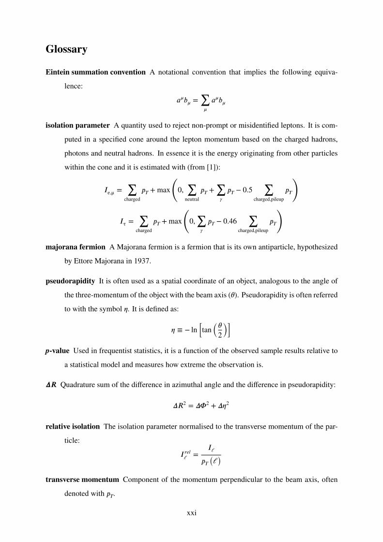
Eintein summation convention A notational convention that implies the following equiva-

lence:

𝑎𝜇𝑏𝜇 = ∑𝜇

𝑎𝜇𝑏𝜇

isolation parameter A quantity used to reject non-prompt or misidentified leptons. It is com-

puted in a specified cone around the lepton momentum based on the charged hadrons,

photons and neutral hadrons. In essence it is the energy originating from other particles

within the cone and it is estimated with (from [1]):

𝐼e,μ = ∑charged

𝑝𝑇 + max(

0, ∑neutral

𝑝𝑇 + ∑𝛾

𝑝𝑇 − 0.5 ∑charged,pileup

𝑝𝑇)

𝐼τ = ∑charged

𝑝𝑇 + max(

0, ∑𝛾


𝑝𝑇)

majorana fermion A Majorana fermion is a fermion that is its own antiparticle, hypothesized

by Ettore Majorana in 1937.

pseudorapidity It is often used as a spatial coordinate of an object, analogous to the angle of

the three-momentum of the object with the beam axis (𝜃). Pseudorapidity is often referred

to with the symbol 𝜂. It is defined as:

𝜂 ≡ − ln [tan(𝜃2)]

p-value Used in frequentist statistics, it is a function of the observed sample results relative to

a statistical model and measures how extreme the observation is.

𝛥𝑅 Quadrature sum of the difference in azimuthal angle and the difference in pseudorapidity:

𝛥𝑅2 = 𝛥𝛷2 + 𝛥𝜂2

relative isolation The isolation parameter normalised to the transverse momentum of the par-

ticle:

𝐼 𝑟𝑒𝑙ℓ =

𝐼ℓ

𝑝𝑇 (ℓ)

transverse momentum Component of the momentum perpendicular to the beam axis, often

denoted with 𝑝𝑇.

xxi

turn-on curve Usually used in reference to the transverse momentum of an object in conjunc-

tion with trigger and reconstruction. It results from the fact that the trigger is performed

on a simplified object and the reconstruction then smears the transverse momentum spec-

trum of the object (with respect to what the trigger sees). In consequence, the efficiency of

the object as a function of the reconstructed transverse momentum is not a step function,

as usually desired, but is smeared resulting in the so-called turn-on curve.

Acronyms

2HDM Two Higgs Doublet Model

ALICE A Large Ion Collider Experiment

ATLAS A Toroidal Large Hadron Collider Apparatus

CERN European Organization for Nuclear Research

CMS Compact Muon Solenoid

CR Control Region

CSV Combined Secondary Vertex

DAQ Data Acquisition

DQM Data Quality Monitoring

DY Drell-Yan

ECAL Electromagnetic Calorimeter

EWT Electroweak Theory

FOM Figure of Merit

HCAL Hadronic Calorimeter

HLT High-Level Trigger

HPS Hadron Plus Strips

ID Identification

L1 Level–1

LEP Large Electron-Positron Collider

LHC Large Hadron Collider

xxii

LHCb Large Hadron Collider beauty

LHCf Large Hadron Collider forward

LSP Lightest Supersymmetric Particle

MC Monte Carlo

MET Missing Transverse Energy

MoEDAL Monopole and Exotics Detector at the LHC

MSSM Minimal Supersymmetric Standard Model

MVA Multivariate Analysis

NLSP Next to Lightest Supersymmetric Particle

nvtx Number of Vertices

OS Opposite Sign

PDF Parton Distribution Function

PF Particle Flow

pMSSM Phenomenological Minimal Supersymmetric Standard Model

POG Physics Object Group

PS Proton Synchroton

PU Pile-up

PV Primary Vertex

QCD Quantum Chromodynamics

QED Quantum Electrodynamics

SM Standard Model

SMS Simplified Model Spectra

SPS Super Proton Synchroton

SR Signal Region

stau Supersymmetric Tau Partner

SUSY Supersymmetry

TOTEM Total Elastic and diffractive cross section Measurement

xxiii

Chapter 1

Introduction

Physics can be described as the branch of science concerned with the nature and properties

of energy and matter and their interactions. One of the fields of physics at the forefront of

our current knowledge is particle physics. Particle physics deals with elementary particles and

their interactions. The theoretical framework upon which particle physics is built is the so-

called Standard Model (SM) of Elementary Particles and their interactions. Throughout the

years, after many stringent tests, the SM has proven to be an extremely successful theory with

unprecedented agreement with experimental data and also through the prediction of several new

phenomena which have been successfully observed. An essential piece of the SM, which eluded

experimental confirmation for many years, is the electroweak symmetry breaking, manifested

through the so-called Higgs mechanism. The Higgs mechanism predicted the existence of a

neutral scalar particle, the Higgs boson, which couples to all elementary particles, bestowing

them their mass.

Studying particle physics is a challenging prospect since most of the particles under study

are no longer readily found in nature. Ordinary matter is made up of up and down quarks and

electrons, with the photon completing the picture of the readily available elementary particles.

In order to study the other elementary particles, they must be produced. Typically existing for

fleeting moments before decaying to stable elementary particles, requiring their existence to be

inferred. These particles are created, for instance, through the collision of ordinary particles that

have been accelerated, a practical application of the well-known mass-energy equivalence for-

mularised by Einstein, 𝐸 = 𝑚𝑐2. This is achieved through the use of particle accelerators, which

1

collide particles at the centre of large experimental detectors. The collisions of elementary parti-

cles are probabilistic in their nature and are governed by QuantumMechanics. Consequently, the

analysis of the data from the detector is, in its essence, a statistical analysis and many collisions

must be performed in order to obtain meaningful results.

The European Organization for Nuclear Research (CERN) has a long history in the field

of physics, operating particle accelerators since 1957, shortly after its inception in 1954, for

research purposes. Examples of accelerators operated by CERN include the Super Proton Syn-

chroton (SPS), the Large Electron-Positron Collider (LEP) and more recently the Large Hadron

Collider (LHC). The SPS was commissioned in 1976, having been converted into a pp collider

in 1981. Two years later, the SPS was at the centre of the discovery of the W and Z bosons,

the carriers of the weak interaction. The SPS is still in use today as the beam source for several

experiments, including as an injector for the LHC. The LEP was in operation between 1989 and

2000 and was used to perform precision measurements for the electroweak theory. At its end of

life, it was decommissioned to make space for the LHC.

The LHC accelerates protons (and lead-ions), with a designed centre of mass energy of

14TeV. After a rocky start, in 2010 and 2011 LHC was operational at an energy of 7TeV,

having increased the energy to 8TeV in 2012. After a long shutdown in 2013 and 2014, during

which upgrades were performed, the LHC restarted taking data in 2015 at an energy of 13TeV.

One of the main goals in the conception of the LHC was to ascertain whether the Higgs boson

exists or not, in this way completing the picture of the SM. The LHC has 4 main experiments,

where the particle beams are made to collide. The experiments are: A Large Ion Collider Ex-

periment (ALICE); A Toroidal Large Hadron Collider Apparatus (ATLAS); Compact Muon

Solenoid (CMS); and Large Hadron Collider beauty (LHCb). ATLAS and CMS are so-called

general purpose detectors as they strive to have a physics program as encompassing as possible.

ALICE and LHCb are specialised detectors, targeted to specific objectives:

• ALICE is specialised in lead-ion collisions

• LHCb is focused on the study of physics of the bottom quark and thematter/antimatter

asymmetry

Beyond themain experiments, there are several other smaller experiments, such as Large Hadron

Collider forward (LHCf), Monopole and Exotics Detector at the LHC (MoEDAL) and Total

2

Elastic and diffractive cross section Measurement (TOTEM).

CMS is a 21.6m long, 14.6m wide, 14 000 t heavy detector that covers almost the full solid

angle. A distinctive feature of the detector, and inspiration for its name, is the superconducting

solenoid. The magnetic field from the solenoid bends the trajectories of the charged particles

formed in the collisions, this allows the momentum of those particles to be measured. As many

detectors in the High Energy Physics field, CMS has an onion-like structure with several layers

of subdetectors, each targeting a specific type of particle or property of a particle. CMS is able

to record the collision data at a rate of 40MHz, the design frequency of the LHC. Subsequently

the trigger system selects a subset of interesting events to be saved to storage and reconstructed

for analysis, which reduces the rate to a few 100Hz.

Searches for the Higgs boson have been under way for decades, with direct searches being

performed with several particle accelerators, such as: at the SPS (in pp collisions), at the LEP (in

e−e+ collisions), at the Tevatron (in pp collisions) and at the LHC (in pp collisions). Recently,

in 2012, the LHC has discovered a new particle consistent with the Higgs boson. Further results

in 2013 constrained this new particle to be even more Higgs-like. This discovery by the LHC

falls in line with previous discoveries, a very amusing factoid, whereby the bosonic elementary

particles have all been discovered in Europe and the fermionic elementary particles in the anglo-

saxon countries [2]. With the discovery of the Higgs boson, the so-called hierarchy problem is

brought to the forefront of Physics. Several theories have been proposed as solutions to this

problem. Among these theories, the most popular one is known as Supersymmetry (SUSY),

which establishes a new symmetry between bosons and fermions.

This thesis describes a search for the direct pair production of the Supersymmetric Tau Part-

ner (stau) using the CMS detector. The search is sensitive to processes with a final state of miss-

ing transverse energy, one lepton (electron or muon) and one hadronically decaying tau lepton,

with the results being interpreted under a SUSY perspective. The presence of stau pairs would

lead to an excess of events with respect to the SM background. Results are given for 19.7 fb−1

of proton-proton collision data with a centre of mass energy of 8TeV recorded in 2012.

The thesis is structured as follows. The standard model and its minimal supersymmetric ex-

tension are reviewed in Chapter 2. The experimental apparatuses, i.e. the CERNLHC and CMS,

are described in Chapter 3. The software stack, including simulation and reconstructions algo-

3

rithms, has an essential role in complex physics analysis and is briefly discussed in Chapter 4.

The base event selection criteria, the first step of the analysis software, is described in Chapter 5.

Advanced selection criteria, targeted to the signal under study, are described in Chapter 6. A

data-driven fake tau estimation method, crucial for the background estimation, is described in

Chapter 7. The systematic uncertainties and their effects on the analysis are described in Chap-

ter 8. Chapter 9 finishes the thesis, presenting the search results followed by conclusions and a

short discussion of the results obtained.

4

Chapter 2

The Standard Model of Particle Physics

and Supersymmetry

The concept that matter is made from a set of basic building blocks can be traced back to antiq-

uity. For instance, ancient Greek philosophers set up the hypothesis that the universe consists

of “ἄτομα” (atoma), indivisible elementary blocks of matter, from which the modern name of

atom is derived. In modern physics, this concept of elementary blocks of matter is still present.

In particular, in the Standard Model of particle physics it is manifested by the elementary parti-

cles which constitute all matter.

The Standard Model (SM) of particle physics is a theory describing the electromagnetic,

weak and strong interactions of elementary particles. The theoretical and mathematical frame-

work upon which the SM is built is quantum field theory, which combines special relativity and

quantum mechanics. Furthermore, the SM is a gauge theory, respecting a group of symmetries.

Under the SM, a group of particles, or vacuum itself, is determined by the lagrangian density.

The equations of motion of the system can be derived from the lagrangian density, which is a

function of the fields. From a theoretical perspective, the SM is an attractive theory because the

description of the interactions arises naturally from symmetry principles. In particular that the

lagrangian be invariant under certain local unitary transformations, the so-called gauge trans-

formations.

The known particles, summarised in Fig. 2.1, constitute the particle content of the SM. Two

5

classes of particles can be identified:

• Fermions – named from the fact that they are characterised by Fermi-Dirac statistics.

They have half integer spin and are the constituents of matter. The fermions are further

subdivided into 3 families, or generations. Fermions are also subdivided into quarks and

leptons.

• Bosons – named from the fact that they are characterised by Bose-Einstein statistics.

They have integer spin and the exchange of bosons between fermions constitutes interac-

tions between those fermions, i.e. they are the force carriers.

Figure 2.1: Particle content of the Standard Model, taken from [3]

There are four known forces in nature, the electromagnetic force, the weak force, the strong

force and the gravitational force. The gravitational force is, so far, the only force not included

within the framework of the SM. It is the weakest of all the forces, which is reflected in the fact

that its effects are only observed when the objects being considered are massive, such as a planet,

a sun or even a whole galaxy. This weakness of the gravitational force explains why very small

objects, such as elementary particles, have vanishingly small gravitational interactions. Which

is why, for the most part, it can be neglected in microscopic models such as the SM.

The electromagnetic force, is the most familiar of the forces. It is responsible for most of the

phenomena observed during a person’s daily life, ranging from our basic senses up to phenomena

such as electricity, radio and even friction. Its name comes from the fact that it describes both

6

electric and magnetic phenomena. Quantum Electrodynamics (QED) is the field theory which

describes the interactions of charged particles with photons. QED can be considered as the

subset of the SM which accounts for only the electromagnetic force.

The weak force is responsible for radioactive decay, having an essential role in nuclear fission

and nuclear fusion. It is unique among the forces since it allows for mixing of the different

particle generations. The electromagnetic and weak forces are unified under a single force,

called the electroweak force. The field theory describing the electroweak force is Electroweak

Theory (EWT) and, like QED, EWT can be considered a subset of the SM.

The strong force is the strongest amongst the known forces, hence its name. It is a confin-

ing force, binding quarks together to form hadrons (2 quarks form mesons and 3 quarks form

baryons) and binding protons and neutrons together to form the nucleus of atoms. The strong

force has 3 associated charges which form a good analogy with the 3 primary colours when per-

forming charge conservation calculations, hence it is also referred to as the colour force. The

field theory describing the strong force is called Quantum Chromodynamics (QCD). Like EWT,

QCD can be considered another subset of the SM and, up to current knowledge, it does not unify

with the electroweak force.

With this minimal prescription of using EWT and QCD, most known phenomena can be

described. However, EWT and QCD are not enough to account for all measured properties

of the elementary particles since given the symmetries respected by this would-be theory, the

particles would have no mass. This goes against experimental evidence, where only the photon

has been measured, up to a very strict uncertainty, to be massless1 [4]. The particle masses

can be introduced in the theory by breaking the electroweak symmetry through the so-called

Higgs mechanism. The Higgs mechanism predicts the existence of a neutral scalar boson, the

Higgs boson. Until recently, experimental evidence consistent with the Higgs boson had not

been seen. In the summer of 2012, results from the CERN LHC by both the CMS and ATLAS

collaborations reported the discovery of a new boson [5, 6], with further measurements revealing

its consistency with the Higgs boson [7–9].

The SM has revealed an unprecedented agreement between theory and experiment, in some

1It should be noted that the gluon is expected to also be massless, although there are no experimental limits on

its mass.

7

situations with a precision of 10 parts in a billion. Despite all of its successes, there are known

deficiencies in the SM, for instance gravitation is not included. Several theories beyond the SM

have been proposed to tackle its shortcomings. SUSY is one of these theories, introducing a new

symmetry between bosons and fermions. SUSY tackles the so-called hierarchy problem, which

will be elaborated on in section 2.2, and simultaneously provides convenient candidate particles

for dark matter.

A full in depth treatment of the SM and SUSY will not be presented here. Only the most

important and relevant aspects will be shown. A more detailed introduction may be found else-

where [10–13].

2.1 The Standard Model of Particle Physics

2.1.1 Gauge Symmetries

In physics, the concept of a symmetry stems from the assumption that a certain quantity is not

measurable. This is, given that a quantity is not measurable, the equations of motion should

not depend on it and should be invariant under transformations of that quantity. Furthermore,

through Noether’s theorem, it can be shown that each symmetry relates to a conservation law.

Some simple examples are the symmetries of space and time. The assumption that the ori-

gin of the coordinate system cannot be measured implies that the equations of motion should

not depend upon the absolute space-time position. In fact, the equations of motion should be

invariant under space translations, which through Noether’s theorem leads to the conservation

of momentum. In a similar manner, the conservation of energy and of angular momentum can

be obtained from the invariance under time translations and space rotations, respectively. These

symmetries are geometrical in their nature and are easy to understand and visualise. The concept

of a symmetry can be further generalised into, internal symmetries and local symmetries.

Internal symmetries are those whose transformation parameters do not affect the space-time

point 𝑥. The simplest example of an internal symmetry is the phase of a wave function, known

to be a non-measurable quantity. Consequently, the theory should be invariant under a change

8

of phase:

𝛹 (𝑥) → 𝑒𝑖𝜃𝛹 (𝑥) (2.1)

This transformation leaves the space-time point invariant, so it is an internal symmetry.

Through Noether’s Theorem, invariance under a change of phase implies the conservation of

the probability current.

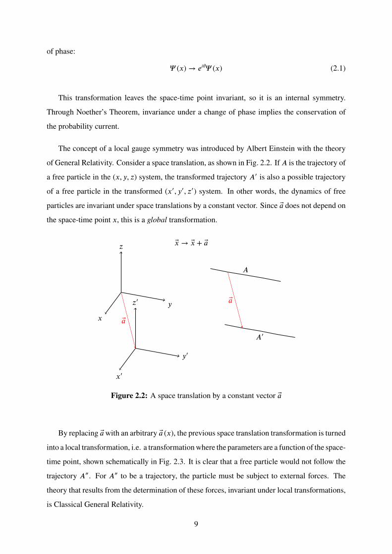
The concept of a local gauge symmetry was introduced by Albert Einstein with the theory

of General Relativity. Consider a space translation, as shown in Fig. 2.2. If 𝐴 is the trajectory of

a free particle in the (𝑥, 𝑦, 𝑧) system, the transformed trajectory 𝐴′ is also a possible trajectory

of a free particle in the transformed (𝑥′, 𝑦′, 𝑧′) system. In other words, the dynamics of free

particles are invariant under space translations by a constant vector. Since 𝑎 does not depend on

the space-time point 𝑥, this is a global transformation.

𝑥

𝑦

𝑧

𝑥′

𝑦′

𝑧′

𝑎

𝐴

�� → �� + 𝑎

𝑎

𝐴′

Figure 2.2: A space translation by a constant vector 𝑎

By replacing 𝑎 with an arbitrary 𝑎 (𝑥), the previous space translation transformation is turned

into a local transformation, i.e. a transformationwhere the parameters are a function of the space-

time point, shown schematically in Fig. 2.3. It is clear that a free particle would not follow the

trajectory 𝐴″. For 𝐴″ to be a trajectory, the particle must be subject to external forces. The

theory that results from the determination of these forces, invariant under local transformations,

is Classical General Relativity.

9

𝑥

𝑦

𝑧

𝑥″

𝑦″

𝑧″

𝑎 (��, 𝑡)

𝐴

�� → �� + 𝑎 (��, 𝑡)

𝐴″

Figure 2.3: A space translation by a space-time dependent vector 𝑎 (𝑥)

Returning to the example of the phase of a wave function, the lagrangian for a free half-spin

fermion, the Dirac Lagrangian, is given by Eq. 2.2, where the Eintein summation convention is

used, 𝛾𝜇 are the four Dirac matrices, 𝛹 = 𝛹 (𝑥) is the Dirac spinor describing the (particle) field

and 𝑚 is the mass of the particle. The Dirac Lagrangian is invariant under internal transforma-

tions, for example the phase transformation, Eq. 2.1. The phase transformation can be made into

a local transformation by replacing 𝜃 with 𝜃 (𝑥), Eq. 2.3. However, the Dirac Lagrangian is not

invariant under this transformation.

ℒ = �� (𝑖𝛾𝜇𝜕𝜇 − 𝑚) 𝛹 (2.2)

𝛹 (𝑥) → 𝑒𝑖𝜃(𝑥)𝛹 (𝑥) (2.3)

The Dirac Lagrangian is not invariant under local transformations because the derivative

term in Eq. 2.2 gives rise to a term proportional to 𝜕𝜇𝜃 (𝑥). In order to restore gauge invari-

ance, the equation must be modified, by replacing the derivative, 𝜕𝜇, for the covariant derivative

Eq. 2.4, where 𝑒 is an arbitrary real constant and a new field, 𝐴𝜇 = 𝐴𝜇 (𝑥), is introduced which

must undergo the transformation in Eq. 2.5 under a gauge transformation. 𝐷𝜇 is called the co-

variant derivative because it satisfies Eq. 2.6.

𝐷𝜇 = 𝜕𝜇 + 𝑖𝑒𝐴𝜇 (2.4)

𝐴𝜇 (𝑥) → 𝐴𝜇 (𝑥) − 1𝑒

𝜕𝜇𝜃 (𝑥) (2.5)

10

𝐷𝜇 [𝑒𝑖𝜃(𝑥)𝛹 (𝑥)] = 𝑒𝑖𝜃(𝑥)𝐷𝜇𝛹 (𝑥) (2.6)

The gauge invariant Dirac Lagrangian is given by Eq. 2.7, which describes the interaction of a

charged spinor field with an external electromagnetic field. Replacing the derivative operator by

the covariant derivative turned the Dirac Lagrangian into the same equation but in the presence

of an external electromagnetic field, represented by the field 𝐴𝜇.

ℒ = �� (𝑖𝛾𝜇𝐷𝜇 − 𝑚) 𝛹 (2.7)

= �� (𝑖𝛾𝜇𝜕𝜇 − 𝑒𝛾𝜇𝐴𝜇 − 𝑚) 𝛹

The complete picture can be obtained by including into Eq. 2.7 the lagrangian density cor-

responding to the degrees of freedom of the electromagnetic field itself. The form for these

degrees of freedom is uniquely determined by the gauge invariance, in a similar manner to what

was shown for the Dirac Lagrangian. Adding these terms to Eq. 2.7 results in:

ℒ = −14

𝐹𝜇𝜈 (𝑥) 𝐹 𝜇𝜈 (𝑥) + �� (𝑥) (𝑖𝛾𝜇𝐷𝜇 − 𝑚) 𝛹 (𝑥) (2.8)

with

𝐹𝜇𝜈 (𝑥) = 𝜕𝜇𝐴𝜈 (𝑥) − 𝜕𝜈𝐴𝜇 (𝑥) (2.9)

In summary, the starting theory, invariant under a group 𝑈 (1) of global phase transforma-

tions, was extended to have a local invariance, interpreted as a 𝑈 (1) symmetry at each point

𝑥. This extension, achieved through a purely geometrical requirement, implies the introduc-

tion of new interactions. Without it being introduced in the original theory, these “geometrical”

interactions describe the well-known electromagnetic forces.

The transformations of the 𝑈 (1) group commute, consequently the 𝑈 (1) group is a so-called

Abelian group. A useful generalisation is the extension of the previous formalism to non-Abelian

groups. However, this is a non-trivial task, first discovered by trial and error, and goes beyond

the scope of this thesis. Despite this, the results of such a generalisation are necessary to write

the SM lagrangian.

11

2.1.2 Spontaneous Symmetry Breaking

Let 𝜙 (𝑥) be a classical complex scalar field, the classical lagrangian density describing the

dynamics is given by Eq. 2.10. This lagrangian is invariant under the group 𝑈 (1) of global

transformations, Eq. 2.11.

ℒ1 = (𝜕𝜇𝜙) (𝜕𝜇𝜙∗) − 𝑀2𝜙𝜙∗ − 𝜆 (𝜙𝜙∗)2 (2.10)

𝜙 (𝑥) → 𝑒𝑖𝜃𝜙 (𝑥) (2.11)

The second two terms of Eq. 2.10 correspond to the potential, Eq. 2.12. The ground state

of the system corresponds to the minimum of 𝑉 (𝜙). The minimum only exists if 𝜆 > 0 and the

position of the minimum depends on the sign of 𝑀2, see Fig. 2.4.

𝑉 (𝜙) = 𝑀2𝜙𝜙∗ + 𝜆 (𝜙𝜙∗)2 (2.12)

(a) 𝑀2 = 4 (b) 𝑀2 = −4

Figure 2.4: The potential 𝑉 (𝜙), with 𝜆 = 1 and |𝑀2| = 4

For 𝑀2 > 0, the minimum is at 𝜙 = 0, a symmetric solution shown in Fig. 2.4a. For 𝑀2 < 0

the solution is still symmetric but there is a circle of minima with radius 𝑣 = (−𝑀2/2𝜆)1/2,

Fig. 2.4b. Each point on the circle of minima is a ground state with the same energy, i.e. the

minima is degenerate and the ensemble of ground states is symmetric. Given the degeneracy

of the ground state, a physical system at its minimal energy configuration must take one of the

points on the circle. By “choosing” one of these points, the system is no longer in a symmetric

situation and in this way the symmetry is spontaneously broken.

12

It can be useful to express the lagrangian around a given ground state, to this effect the field 𝜙

is translated. This transformation does not lead to a loss of generality since any point on the circle

of minima can be obtained from any other given point by the transformation in Eq. 2.11. It is

convenient to choose a point along the real axis in the 𝜙-plane for the translation. Consequently,

the field is written as Eq. 2.13. The lagrangian, Eq. 2.10, is then expressed as Eq. 2.14.

𝜙 (𝑥) = 1√2

[𝑣 + 𝜓 (𝑥) + 𝑖𝜒 (𝑥)] (2.13)

ℒ1 (𝜙) → ℒ2 (𝜓, 𝜒) = 12 (𝜕𝜇𝜓)

2 + 12 (𝜕𝜇𝜒)

2 − 12 (2𝜆𝑣2) 𝜓2

− 𝜆𝑣𝜓 (𝜓2 + 𝜒2) − 14 (𝜓2 + 𝜒2)

2(2.14)

The lagrangians ℒ1 and ℒ2 are completely equivalent and describe the dynamics of the same

physical system. However, one can be more suitable to resolve certain classes of problems than

the other. For instance, when using perturbation theory ℒ2 is more likely to give sensible results,

since ℒ1 is described around an unstable point, a local maximum. The lagrangian ℒ2 can be

interpreted as describing a quantum system which consists of two interacting scalar particles,

one with mass 𝑚2𝜓 = 2𝜆𝑣2 (the third term in Eq. 2.14) and the other with 𝑚𝜒 = 0, a so-called

massless Goldstone boson.

In the presence of a gauge symmetry, spontaneous symmetry breaking leads to an interest-

ing result. As in section 2.1.1, the lagrangian ℒ1 is made gauge invariant by promoting the

𝑈 (1) symmetry to a gauge symmetry, with 𝜃 → 𝜃 (𝑥), and replacing the derivative operator 𝜕𝜇

with the covariant derivative 𝐷𝜇. As previously described, this implies the introduction of a

massless vector field, 𝐴𝜇, which can be called the “photon”. The photon kinetic energy term is

also introduced, and Eq. 2.15 is obtained, which is invariant under the gauge transformation in

Eq. 2.16.

ℒ1 → ℒ1 = −14

𝐹 2𝜇𝜈 + |(𝜕𝜇 + 𝑖𝑒𝐴𝜇) 𝜙|

2 − 𝑀2𝜙𝜙∗ − 𝜆 (𝜙𝜙∗)2 (2.15)

𝜙 (𝑥) → 𝑒𝑖𝜃(𝑥)𝜙 (𝑥) ; 𝐴𝜇 → 𝐴𝜇 − 1𝑒

𝜕𝜇𝜃 (𝑥) (2.16)

Spontaneous symmetry breaking of the 𝑈 (1) symmetry only occurs if 𝜆 > 0 and 𝑀2 < 0, as

seen previously. In the currently described situation, it is more useful to perform the translation

of the complex field using polar coordinates rather than Cartesian ones. The field is then written

as Eq. 2.17. Taking advantage of gauge invariance, the vector field is written in an adequate

13

gauge Eq. 2.18, since this does not affect the equations of motion. With this notation, the gauge

transformation Eq. 2.16 is simply a translation of the field 𝜁.

𝜙 (𝑥) = 1√2

[𝑣 + 𝜌 (𝑥)] 𝑒𝑖𝜁(𝑥)/𝑣 (2.17)

𝐴𝜇 (𝑥) = 𝐵𝜇 (𝑥) − 1𝑒𝑣

𝜕𝜇𝜁 (𝑥) (2.18)

𝜁 (𝑥) → 𝜁 (𝑥) + 𝑣𝜃 (𝑥) (2.19)

Replacing Eq. 2.17 and Eq. 2.18 into Eq. 2.15 the gauge invariant translated lagrangian is

obtained.

ℒ1 → ℒ2 = −14

𝐵2𝜇𝜈 + 𝑒2𝑣2

2𝐵2

𝜇 + 12 (𝜕𝜇𝜌)

2 − 12 (2𝜆𝑣2) 𝜌2

− 𝜆4

𝜌4 + 12

𝑒2𝐵2𝜇 (2𝑣𝜌 + 𝜌2)

(2.20)

𝐵𝜇𝜈 = 𝜕𝜇𝐵𝜈 − 𝜕𝜈𝐵𝜇

The lagrangian ℒ2 does not depend on 𝜁 (𝑥) and the formula describes twomassive particles,

a vector 𝐵𝜇 and a scalar 𝜌. This is the interesting result, alluded to earlier. In essence, the ini-

tially massless gauge vector boson acquired a mass from the introduction of the scalar symmetry

breaking potential. Simultaneously, the would-be Goldstone boson, which originated from the

symmetry breaking, no longer appears. The degrees of freedom of the Goldstone boson were

used to make the transition from massless to massive vector bosons, i.e. the Goldstone bosons

were “swallowed” by the massless vector bosons. As previously, this result can be extended to

the non-Abelian case, but goes beyond the scope of this thesis.

2.1.3 Building the Standard Model

In order to build the SM, choosing the set of symmetries respected by the model is the first step.

This is done by specifying the gauge group. Each generator of the group gives rise to a gauge

boson, this was implicit in the previous sections but can be explicitly seen in the full treatment

of non-Abelian gauge groups. From experimental results, it is known that the weak force has 3

associated bosons: the Z boson [14] and the W± bosons [15, 16]; and that the electromagnetic

force has a single associated boson, the photon (γ). Given that the electromagnetic and weak

14

forces are unified under the electroweak force, its corresponding gauge group is the only non-

trivial group with 4 generators; 𝑈 (1) × 𝑆𝑈 (2). EWT is the theory describing only these two

forces, subject to the mentioned gauge group. There are two quantum numbers originating from

the generators of the gauge group. These quantum numbers are analogous to the well-known

electric charge (𝑄). The first, the weak hypercharge quantum number (𝑌), corresponds to the

generator of 𝑈 (1). The generators of 𝑆𝑈 (2) do not commute among each other, consequently

only one can be taken as a quantum number. It is customary to choose the third generator of

𝑆𝑈 (2) as the weak isospin quantum number (𝑇3).

The inclusion of the strong force is more complex and will not be treated in full here. The

simplest way to identify the associated gauge group would be to consider that for the model to

be coherent, there must be 3 charge types associated to the strong force2. Thus, the simplest

group associated with the strong force is 𝑆𝑈 (3). The 𝑆𝑈 (3) group has 8 generators and as a

result there are 8 bosons (gluons) associated to the strong force. Therefore, the gauge group of

the SM is 𝑈 (1) × 𝑆𝑈 (2) × 𝑆𝑈 (3).

With this choice of the SM gauge group, the electric charge operator, 𝑄, is defined by a

linear combination of the weak hypercharge, 𝑌, and the third component of the weak isospin, 𝑇3,

summarised in Eq. 2.21 where the coefficient in front of 𝑌 is arbitrary and fixes the normalisation

of the 𝑈 (1) generator relative to those of 𝑆𝑈 (2).

𝑄 = 𝑇3 + 12

𝑌 (2.21)

The next step is to choose the fields of the elementary particles and assign them to repre-

sentations of the gauge group. The number and the interaction properties of the bosons are

completely specified by the gauge group. For the fermions, we could in principle choose any

number and assign any representation. In practice, the choice is guided by observation, which,

in fact, restricts the choice. The observed particles are summarised in Fig. 2.1. As can be seen

in the figure, there are 12 fermions, 6 leptons and 6 quarks. The fermions are simultaneously

subdivided into three generations (or families). Each generation consists of 2 leptons and 2

quarks, with each generation sequentially heavier than the previous. The three generations are

in all other aspects the same; the two leptons are classified into one lepton with charge −1 and2The requirement of 3 charge types is related to the cancellation of triangle anomalies, mentioned further on.

The requirement results from the assumption of the electric charge of the quarks.

15

the other with charge 0; the two quarks are classified into one quark with charge −1⁄3 and the

other with charge +2⁄3. There is no known reason why nature repeats the generations thrice. The

simplest representation of the fermions that incorporates this repetition is to choose a specific

representation for the first generation and repeat it for the others.

Given the experimental evidence that the charged W bosons only couple to the left-handed

components of the particle fields, the left-handed fields are assigned to doublets of 𝑆𝑈 (2). The

right-handed components are assigned to singlets of 𝑆𝑈 (2). This assignment determines the

𝑆𝑈 (2) transformation properties of the fermion fields. It also fixes their 𝑌 charges, and therefore

their 𝑈 (1) properties, using Eq. 2.21. Given the interaction of the quarks with the strong force,

the quarks are assigned to triplets of 𝑆𝑈 (3), whereas given that the leptons do not interact under

the strong force they are assigned to singlets of 𝑆𝑈 (3). Henceforth the symbol for a given

particle will be used for its associated Dirac field.

The projection operators (left-handed: 12 (1 − 𝛾5); right-handed:

12 (1 + 𝛾5)) are used to sep-

arate the right-handed from the left-handed fields. The fields in the lepton sector become:

𝛹 𝑖𝐿 (𝑥) = 1

2 (1 − 𝛾5)⎛⎜⎜⎝

𝜈𝑖 (𝑥)

ℓ−𝑖 (𝑥)

⎞⎟⎟⎠

; 𝑖 = 1, 2, 3 (2.22)

𝑅𝑖 (𝑥) ≡ ℓ−𝑖𝑅 (𝑥) = 1

2 (1 + 𝛾5) ℓ−𝑖 (𝑥) (2.23)

𝜈𝑖𝑅 (𝑥) = 12 (1 + 𝛾5) 𝜈𝑖 (𝑥) (2.24)

Where 𝑖 is the family index and the last equation is included, here only, for completeness,

since there is no experimental evidence for right handed neutrinos. The fields ℓ−𝑖 are the charged

lepton fields and 𝜈𝑖 the neutrino fields. 𝑅𝑖 is the charged right-handed lepton field and the field

𝛹 𝑖𝐿 is a doublet of 𝑆𝑈 (2) of the left handed lepton fields, 𝜈𝑖𝑅 is the would-be right-handed

neutrino field. The transformation properties of these fields under local 𝑆𝑈 (2) transformations

are given by Eq. 2.25, where 𝜏 are the three generators of the 𝑆𝑈 (2) group. Since the leptons

are singlets under 𝑆𝑈 (3), they are not affected by local 𝑆𝑈 (3) transformations, as a result their

transformations are given by Eq. 2.26.

𝛹 𝑖𝐿 (𝑥) → 𝑒𝑖𝜏⋅𝜃(𝑥)𝛹 𝑖

𝐿 (𝑥) ; 𝑅𝑖 (𝑥) → 𝑅𝑖 (𝑥) (2.25)

𝛹 𝑖𝐿 (𝑥) → 𝛹 𝑖

𝐿 (𝑥) ; 𝑅𝑖 (𝑥) → 𝑅𝑖 (𝑥) (2.26)

16

Given the 𝑌 normalisation set by Eq. 2.21, the 𝑈 (1) charge of the lepton fields is uniquely

determined and, as a result, the transformation properties of the fields under local 𝑈 (1) trans-

formations.

𝑌 (𝛹 𝑖𝐿) = −1; 𝑌 (𝑅𝑖) = −2 (2.27)

If a right-handed neutrino were to exist it would have 𝑌 (𝜈𝑖𝑅) = 0, which, in conjunction

with it being a singlet under 𝑆𝑈 (2) and 𝑆𝑈 (3), would imply that it does not couple to any

gauge boson. Thus it would be near impossible to detect since it would only interact with the

Higgs boson.

In the quark sector, the fields are given by Eq. 2.28, Eq. 2.29 and Eq. 2.30, where 𝑖 is the

family index and an index for the colour is not explicitly written. The fields 𝑈 𝑖 are the up-type

quarks fields and 𝐷𝑖 the down-type quark fields. 𝑈 𝑖𝑅 and 𝐷𝑖

𝑅 are the right-handed fields for the

up-type and down-type quark fields, respectively and𝑄𝑖𝐿 is a doublet of𝑆𝑈 (2) of the left-handed

quark fields.

𝑄𝑖𝐿 (𝑥) = 1

2 (1 − 𝛾5)⎛⎜⎜⎝

𝑈 𝑖 (𝑥)

𝐷𝑖 (𝑥)

⎞⎟⎟⎠

; 𝑖 = 1, 2, 3 (2.28)

𝑈 𝑖𝑅 (𝑥) = 1

2 (1 + 𝛾5) 𝑈 𝑖 (𝑥) (2.29)

𝐷𝑖𝑅 (𝑥) = 1

2 (1 + 𝛾5) 𝐷𝑖 (𝑥) (2.30)

Under local 𝑆𝑈 (2) transformations, the quark fields transform in a similar manner to the

lepton fields, Eq. 2.31. However, under local 𝑆𝑈 (3) transformations, the quark fields transform

according to Eq. 2.32, with 𝑡𝐶 = 12𝜆𝐶 where 𝜆 are the eight generators of 𝑆𝑈 (3) and 𝐶 runs from

1 to 8.

𝑄𝑖𝐿 (𝑥) → 𝑒𝑖𝜏⋅𝜃(𝑥)𝑄𝑖

𝐿 (𝑥) ; 𝑈 𝑖𝑅 (𝑥) → 𝑈 𝑖

𝑅 (𝑥) ; 𝐷𝑖𝑅 (𝑥) → 𝐷𝑖

𝑅 (𝑥) (2.31)

𝑄𝑖𝐿 (𝑥) → 𝑒𝑖��⋅𝛽(𝑥)𝑄𝑖

𝐿 (𝑥) ; 𝑈 𝑖𝑅 (𝑥) → 𝑒𝑖��⋅𝛽(𝑥)𝑈 𝑖

𝑅 (𝑥) ; 𝐷𝑖𝑅 (𝑥) → 𝑒𝑖��⋅𝛽(𝑥)𝐷𝑖

𝑅 (𝑥) (2.32)

The 𝑈 (1) charge of the quark fields, computed with Eq. 2.21, is:

𝑌 (𝑄𝑖𝐿) = 1

3; 𝑌 (𝑈 𝑖

𝑅) = 43

; 𝑌 (𝐷𝑖𝑅) = −2

3(2.33)

For the choice of the Higgs scalar fields, the option with the minimal number of fields is

taken. From experimental evidence, it is known that three of the four 𝑈 (1) × 𝑆𝑈 (2) vector

17

gauge bosons must acquire a mass through the breaking of the electroweak symmetry. As seen

in Section 2.1.2, in order to transition from a massless vector gauge boson to a massive one, a

Goldstone boson must be “swallowed” by the vector gauge boson. Consequently, three Gold-

stone bosons are necessary. The minimal number of scalar fields necessary to accommodate the

above is four, two charged and two neutral. The fields are chosen to be placed into a complex

doublet under 𝑆𝑈 (2).

𝛷 =⎛⎜⎜⎝

𝜙+

𝜙0

⎞⎟⎟⎠

; 𝛷 (𝑥) → 𝑒𝑖𝜏⋅𝜃𝛷 (𝑥) (2.34)

The 𝑈 (1) charge of 𝛷 is 𝑌 (𝛷) = 1.

The choice of fields and their representations are summarised in Table 2.1. The fields for

right-handed particles have been replaced with the field for the corresponding left-handed an-

tiparticles. For completeness, the gauge fields are also listed.

From this point onward, no more choices remain since all subsequent steps are uniquely

determined by the previous choices, i.e. the gauge group, the particle fields and their represen-

tation under transformations of the gauge group. The most general renormalisable lagrangian,

involving the fields in Eq. 2.22, Eq. 2.23, Eq. 2.28, Eq. 2.29, Eq. 2.30 and Eq. 2.34, invariant

under gauge transformations of 𝑈 (1)×𝑆𝑈 (2)×𝑆𝑈 (3) is written. The result, Eq. 2.35, has been

split into the several separate contributions, which will be elaborated on individually.

ℒ = ℒfree+interaction + ℒGauge + ℒHiggs + ℒYukawa (2.35)

ℒfree+interaction =3

∑𝑖=1

[�� 𝑖𝐿𝑖𝛾𝜇𝐷𝜇𝛹 𝑖

𝐿 + ��𝑖𝑖𝛾𝜇𝐷𝜇𝑅𝑖 + ��𝑖𝐿𝑖𝛾𝜇𝐷𝜇𝑄𝑖

𝐿

+�� 𝑖𝑅𝑖𝛾𝜇𝐷𝜇𝑈 𝑖

𝑅 + ��𝑖𝑅𝑖𝛾𝜇𝐷𝜇𝐷𝑖

𝑅] (2.36)

ℒGauge = −14

𝐵𝜇𝜈𝐵𝜇𝜈 − 14

��𝜇𝜈 ⋅ �� 𝜇𝜈 − 14

��𝜇𝜈 ⋅ ��𝜇𝜈 (2.37)

ℒHiggs = |𝐷𝜇𝛷|2 − 𝑉 (𝛷) (2.38)

−ℒYukawa =3

∑𝑖=1

[𝐺𝑖 (�� 𝑖𝐿𝑅𝑖𝛷 + ℎ.𝑐.)] +

3

∑𝑖=1

[𝐺𝑖𝑢 (��𝑖

𝐿𝑈 𝑖𝑅�� + ℎ.𝑐.)]

+3

∑𝑖,𝑗=1

[(��𝑖𝐿𝐺𝑖𝑗

𝑑 𝐷𝑗𝑅𝛷 + ℎ.𝑐.)] (2.39)

18

Table 2.1: Field content of the Standard Model. The column representa-

tion indicates under which representations of the gauge group each field

transforms, in the order (𝑆𝑈 (3) , 𝑆𝑈 (2) , 𝑈 (1)). Superscript 𝐶 denotes

an antiparticle; for the 𝑈 (1) group the value of the weak hypercharge is

listed instead.

Gauge Fields – Spin 1

Symbol Associated Charge Group Coupling Representation

𝐵 Weak Hypercharge 𝑈 (1) 𝑔′ (1, 1, 0)

𝑊 𝑖 Weak Isospin 𝑆𝑈 (2) 𝑔𝑤 (1, 3, 0)

𝐺𝑖 Colour 𝑆𝑈 (3) 𝑔𝑠 (8, 1, 0)

Fermion Fields – Spin 12

Symbol Name Representation

𝑄𝑖𝐿 Left-handed quark (3, 2, 1

3)𝑈 𝑖

𝑅𝐶 Left-handed antiquark (up) (3, 1, − 4

3)𝐷𝑖

𝑅𝐶 Left-handed antiquark (down) ( 3, 1, 2

3)𝛹 𝑖

𝐿 Left-handed lepton (1, 2, −1)

𝑅𝑖𝐶 Left-handed antilepton (1, 1, 2)

Higgs Fields – Spin 0

Symbol Name Representation

𝛷 Higgs boson (1, 2, 1)

The “free+interaction” term, Eq. 2.36, corresponds to the gauge invariant Dirac Lagrangian.

This term describes the free fermions and their interactions with the aforementioned gauge fields.

The covariant derivatives are determined by the assumed transformation properties of the fields

19

and are given by:

𝐷𝜇𝛹 𝑖𝐿 = (𝜕𝜇 −𝑖𝑔𝑤

𝜏2

⋅ ��𝜇 +𝑖𝑔′

2𝐵𝜇) 𝛹 𝑖

𝐿 (2.40)

𝐷𝜇𝑅𝑖 = (𝜕𝜇 +𝑖𝑔′𝐵𝜇) 𝑅𝑖 (2.41)

𝐷𝜇𝑄𝑖𝐿 = (𝜕𝜇 −𝑖𝑔𝑠�� ⋅ ��𝜇 −𝑖𝑔𝑤

𝜏2

⋅ ��𝜇 −𝑖𝑔′

6𝐵𝜇) 𝑄𝑖

𝐿 (2.42)

𝐷𝜇𝑈 𝑖𝑅 = (𝜕𝜇 −𝑖𝑔𝑠�� ⋅ ��𝜇 −𝑖2

3𝑔′𝐵𝜇)𝑈 𝑖

𝑅 (2.43)

𝐷𝜇𝐷𝑖𝑅 = (𝜕𝜇 −𝑖𝑔𝑠�� ⋅ ��𝜇 +𝑖

𝑔′

3𝐵𝜇) 𝐷𝑖

𝑅 (2.44)

The gauge term, Eq. 2.37, corresponds to the kinetic energy terms for the vector fields, which

is fully constrained by the chosen gauge group. This term also describes the self-interactions of

the 𝑊𝜈 and 𝐺𝜈 fields, which arise from the non-Abelian structure of the corresponding gauge

groups, 𝑆𝑈 (2) and 𝑆𝑈 (3) respectively. The field strengths 𝐵𝜇𝜈, ��𝜇𝜈 and ��𝜇𝜈 are given by:

𝐵𝜇𝜈 (𝑥) = 𝜕𝜇𝐵𝜈 (𝑥) − 𝜕𝜈𝐵𝜇 (𝑥) (2.45)

��𝜇𝜈 (𝑥) = 𝜕𝜇��𝜈 (𝑥) − 𝜕𝜈��𝜇 (𝑥) + 𝑖𝑔𝑤 (��𝜇 (𝑥) ��𝜈 (𝑥) − ��𝜈 (𝑥) ��𝜇 (𝑥)

2 )(2.46)

��𝜇𝜈 (𝑥) = 𝜕𝜇��𝜈 (𝑥) − 𝜕𝜈��𝜇 (𝑥) + 𝑖𝑔𝑠 (��𝜇 (𝑥) ��𝜈 (𝑥) − ��𝜈 (𝑥) ��𝜇 (𝑥)) (2.47)

The Higgs term, Eq. 2.38, introduces the Higgs potential into the SM lagrangian, describes

the dynamics of the Higgs field and its interaction with the gauge bosons. The most general

Higgs potential compatible with the transformation properties of the field 𝛷 is given by Eq. 2.48.

The covariant derivative, like for the fermion fields, is determined by the assumed transformation

properties of the field and is given by Eq. 2.49.

𝑉 (𝛷) = 𝜇2𝛷†𝛷 + 𝜆 (𝛷†𝛷)2 (2.48)

𝐷𝜇𝛷 = (𝜕𝜇 − 𝑖𝑔𝑤𝜏2

⋅ ��𝜇 − 𝑖𝑔′

2𝐵𝜇) 𝛷 (2.49)

The last term in Eq. 2.35, Eq. 2.39, describes the coupling between the scalar 𝛷 and the

fermions, a so-called Yukawa coupling. In the absence of right handed neutrinos, this is the

most general term. If right handed neutrinos exist, another Yukawa coupling term would be

included, similar to the first term, with 𝑅𝑖 replaced by 𝜈𝑖𝑅 and 𝛷 by �� which is proportional to

𝜏2𝛷∗. Which, in conjunction with Eq. 2.24, shows that the SM can accommodate a right-handed

20

neutrino, but it would only couple to the Higgs field. The part of the Yukawa Lagrangian relating

to the quarks requires a more in depth explanation. In general any basis in the quark family space

can be chosen. There are two Yukawa terms, one for the up-type quarks, 𝑈 𝑖𝑅, and the other for the

down-type quarks, 𝐷𝑖𝑅. Given the non-conservation of the individual quark quantum numbers,

there is no explicit pairing between the up-type and down-type quarks. As a result, in general

it is not possible to simultaneously diagonalise both Yukawa terms, which requires at least one

of the Yukawa terms to have non-diagonal terms which mix the families. By convention, the

off-diagonal terms are attributed to the down-type quark space, as seen by the sum over two

indexes in Eq. 2.39.

Of note in the SM lagrangian is that the ��𝜇, ��𝜇 and𝐵𝜇 gauge bosons appear to bemassless as

well as all the fermions. With the lagrangian defined, the next step is to choose the 𝜇2 parameter

of the Higgs potential to be negative, in this way triggering spontaneous symmetry breaking, as

described in section 2.1.2. As a result, the minimum of the Higgs potential occurs at a distance

of 𝑣 from the origin, with 𝑣2 = −𝜇2/𝜆. Translating the Higgs field by a constant along the real

axis of the 𝛷-plane, Eq. 2.50, generates new terms in the lagrangian.

𝛷 → 𝛷 + 1√2

⎛⎜⎜⎝

0

𝑣

⎞⎟⎟⎠

(2.50)

The mass terms are among the most noteworthy of the generated new terms. The Higgs

mass is taken from the coefficient of the quadratic part of 𝑉 (𝛷) after the translation of the field,

the mass is given by Eq. 2.51. The fermion masses arise from the Yukawa term, for the leptons

the mass is given by Eq. 2.52. The three arbitrary constants 𝐺ℓ can be chosen such that the

three observed masses of the leptons are obtained. The mass terms for the quarks must take into

account the family mixing which results from the Yukawa term in the lagrangian, Eq. 2.39. For

the up-type quarks, the masses are given by Eq. 2.53, which in semblance to the leptons can

accommodate the three observed masses since there are three arbitrary constants 𝐺𝑞u. For the

down-type quarks a three-by-three mass matrix is obtained, Eq. 2.54.

𝑚H = √−2𝜇2 = √2𝜆𝑣2 (2.51)

𝑚ℓ = 1√2

𝐺ℓ𝑣 with ℓ = e, μ, τ (2.52)

𝑚𝑞 = 𝐺𝑞u𝑣 with 𝑞 = u, c, t (2.53)

𝑚𝑞 = 𝐺𝑖𝑗d 𝑣 (2.54)

21

It is usual to work in a space where themasses are diagonal, the basis of the down-type quarks

must then be changed such that 𝐺𝑖𝑗d is diagonal. This can be done with a three-by-three unitary

matrix, 𝑉, such that 𝑉 †𝐺𝑖𝑗d 𝑉 = diag. The quark masses would then be given by 𝑚𝑞 = 𝐺𝑞

d𝑣, with

𝑞 = d, s, b, which also accommodates for the three observed down-type quark masses with the

three arbitrary constants 𝐺𝑞d.

With this formulation, the matrix 𝑉 encodes additional arbitrary constants. In general, a 3×3

complex matrix has 18 degrees of freedom (9 real and 9 imaginary), however the requirement to

be unitary, 𝑉 𝑉 † = 1, constrains 9 of the parameters. Invariance under phase transformations of

the quark fields constrains a further 5 of the remaining 9 parameters. Consequently, the matrix

𝑉 has 4 degrees of freedom, 3 of which can be identified as Euler rotation angles and the fourth

as an arbitrary phase, it is traditionally written in the form:

𝑉 =

⎛⎜⎜⎜⎜⎝

𝑐1 𝑠1𝑐3 𝑠1𝑠3

−𝑠1𝑐3 𝑐1𝑐2𝑐3 − 𝑠2𝑠3𝑒𝑖𝛿 𝑐1𝑐2𝑠3 + 𝑠2𝑐3𝑒𝑖𝛿

−𝑠1𝑠2 𝑐1𝑠2𝑐3 + 𝑐2𝑠3𝑒𝑖𝛿 𝑐1𝑠2𝑠3 − 𝑐2𝑐3𝑒𝑖𝛿

⎞⎟⎟⎟⎟⎠

(2.55)

with the shorthand notation 𝑐𝑘 = cos 𝜃𝑘, 𝑠𝑘 = sin 𝜃𝑘, 𝑘 = 1, 2, 3. The phase, 𝛿, is a natural

source for CP, or T, violation, which a model with only two generations, or four quarks, does

not allow. This matrix was first introduced by Kobayashi and Masukawa as an extension to the

Cabibbo matrix, precisely because of the CP violation it allows. For this reason, this matrix is

often called the Cabibbo–Kobayashi–Maskawa (CKM) matrix.

The mass terms for the gauge bosons arise from the |𝐷𝜇𝛷|2 term in the untranslated la-

grangian, i.e. Eq. 2.35. Direct substitution of the covariant derivative and then performing the

translation of the Higgs potential leads to the following quadratic term:

18

𝑣2[𝑔2

𝑤 (𝑊 1𝜇𝑊 1𝜇 + 𝑊 2

𝜇𝑊 2𝜇) + (𝑔′𝐵𝜇 − 𝑔𝑤𝑊 3

𝜇)2] (2.56)

By defining the charged vector bosons as in Eq. 2.57, their masses are obtained from Eq. 2.56

and given by Eq. 2.58. The neutral gauge bosons have a 2 × 2 non-diagonal mass matrix. After

diagonalisation, the mass eigenstates become Eq. 2.59 and the mass eigenvalues are Eq. 2.60.

As expected, one of the neutral bosons remains massless and is identified with the photon.

W±𝜇 =

𝑊 1𝜇 ∓ 𝑖𝑊 2

𝜇

√2(2.57)

𝑚W =𝑣𝑔𝑤

2(2.58)

22

Z𝜇 = cos 𝜃𝑊𝐵𝜇 − sin 𝜃𝑊𝑊 3𝜇

A𝜇 = cos 𝜃𝑊𝐵𝜇 + sin 𝜃𝑊𝑊 3𝜇

with tan 𝜃𝑊 =𝑔′

𝑔𝑤(2.59)

𝑚Z =𝑣√𝑔𝑤

2+𝑔′2

2= 𝑚W

cos 𝜃𝑊

𝑚A = 0(2.60)

The classical SM lagrangian, Eq. 2.35, contains nineteen arbitrary real parameters. They

are:

• the three gauge coupling constants, 𝑔′, 𝑔𝑤, 𝑔𝑠

• the two parameters of the Higgs potential, 𝜆 and 𝜇2

• three Yukawa coupling constants for the three lepton families, 𝐺ℓ with ℓ = e, μ, τ

• six Yukawa coupling constants for the three quark families, 𝐺𝑞u with 𝑞 = u, c, t and

𝐺𝑞d with 𝑞 = d, s, b

• four parameters of the CKM matrix, three angles and a phase

• the QCD theta angle, 𝜃QCD

2.1.4 Success and Shortcomings of the Standard Model

The SM, whose current formulation was finalised in the mid-1970s, has been an extremely wor-

thy theory. It accurately describes most of the present-day data and has had an enormous success

in predicting new phenomena. Predictions of the SM range from the prediction of the existence

and properties of weak neutral currents, confirmed by Gargamelle in 1972 [17], to the prediction

of the Higgs boson, for which a candidate has been discovered in 2012 [5, 6]. The precision tests

of QED constitute one of the most impressive results of the SM, where an agreement between

theory and experiment is found to within 10 parts in a billion (10−8).

Another compelling prediction of the SM dates back to the discovery of the tau lepton (τ),

where upon the discovery of the tau, the b and t quarks were predicted to exist [18]. The pre-

diction results from the fact that a gauge theory, such as the SM, must be anomaly free. The

charged particles in the SM contribute to the so-called triangle anomalies. Requiring the anoma-

lies to cancel corresponds to requiring that the sum of the charges of all the particles in a family

be null. Consequently, discovering the tau lepton, a new family, implied that the third family

23

quarks should exist in order to cancel the triangle anomaly. This same reasoning was used in the

beginning of section 2.1.3 to justify the three colour charges of the quarks.

The success of the SM can be succinctly overviewed in the global electroweak fit of the SM

[19]. The electroweak observable parameters are expressed as a function of the input parameters

of the SM and their observed and predicted values are compared. With the discovery of theHiggs

boson, all input parameters are known, which allows for a full assessment of the consistency of

the SM. Fig. 2.5 summarises the results of the fit, with the pull values for each parameter. None

of the pull values exceed 3𝜎, proving the consistency of the SM. The fit converges to 𝜒2 = 21.8

with 14 degrees of freedom, resulting in a p-value of 0.08.

With all these results, it is safe to say that the SM is among themost stringently tested theories

in physics and has mustered a staggering amount of experimental evidence in its favour.

Despite the unprecedented success of the SM, there are several known issues with the the-

ory. For instance, measurements since 1998 have shown that neutrinos oscillate [20, 21], which

requires them to also have mass. The SM can accommodate massive neutrinos, however there is

no consensus on the mechanism to introduce the neutrino oscillations. The observed overabun-

dance of matter over antimatter can not be explained within the framework of the SM. Even

though the SM does have the mentioned complex phase in the CKMmatrix which allows for CP

violation, the effect is not large enough to explain the observed matter/anti-matter asymmetry

observed in the universe.

Furthermore, the latest results from the Planck telescope experiment have revealed that or-

dinary matter accounts for only about 5% of the mass-energy content of the universe, with dark

matter accounting for slightly more than 26% and dark energy making up the rest [22]. The SM

has no candidate particle for dark matter, and an explanation for the nature of dark energy is still

to be elucidated. Another fundamental flaw with the SM is the fact that gravity is not included

within its framework.

24

measσ) / meas - Ofit

(O

-3 -2 -1 0 1 2 3

)2

Z(M

(5)

hadα∆

tmbmcmb0Rc0R

bAcA

0,bFBA

0,cFBA

)FB

(Qlepteff

Θ2sin

(SLD)lA

(LEP)lA

0,lFBAlep0R

0had

σZΓZM

WΓWMHM 0.0 (-1.5)

-1.2 (-0.3)

0.2 (0.2)

0.2 (0.0)

0.1 (0.3)

-1.7 (-1.7)

-1.1(-1.0)

-0.8 (-0.7)

0.2 (0.4)

-1.9 (-1.7)

-0.7 (-0.8)

0.9 (1.0)

2.5 (2.7)

0.0 (0.0)

0.6 (0.6)

0.0 (0.0)

-2.4 (-2.3)

0.0 (0.0)

0.0 (0.0)

0.4 (0.0)

-0.1 (0.0)

measurementHwith M measurementHw/o M

Plot inspired by Eberhardt et al. [arXiv:1209.1101]

G fitter SM

Feb 13

Figure 2.5: Differences between the SM prediction and the measured parameter, in units of the

uncertainty for the fit including 𝑀H (colour) and without 𝑀H (grey). Figure taken from [19].

2.2 Supersymmetry

The shortcomings of the SM seem to indicate that the SM is an effective theory. Several theories

have been proposed to address these shortcomings, such as Supersymmetry (SUSY), Techni-

color and String Theories.

In a theory beyond the SM, where the Higgs mass is calculable, the radiative corrections

25

to the Higgs boson mass are quadratically divergent. These quadratic divergences must be can-

celled by the bare mass of the Higgs for the theory to be renormalisable. If the theory is to be

valid up to very high energy scales, the cancellation must be very precise which is, in general,

considered a problem and requires fine-tuning. This problem is the so-called hierarchy problem.

The quadratic growth of the Higgs boson mass beyond tree level is one of the motivations behind

the introduction of SUSY.

To understand one of the main motivations for SUSY, consider a simplified theory with both

a massive scalar, 𝜙, and a fermion, 𝜓, in addition to a Higgs field, ℎ, the lagrangian would be:

ℒ ∼ −𝑔𝐹��𝜓ℎ − 𝑔2𝑆ℎ2𝜙 (2.61)

In this theory, the one-loop contributions to the Higgs boson mass are illustrated in Fig. 2.6 and

the terms that contribute to the mass of the Higgs are given in Eq. 2.62.

𝑓H H

(a) Fermion loop

𝑆

H H

(b) Scalar loop

Figure 2.6: One-loop quantum corrections to the Higgs squared mass parameter, 𝑀2H.

𝑀2ℎ ∼ 𝑀2

ℎ0 +𝑔2

𝐹

4𝜋2 (𝛥2 + 𝑚2𝐹) −

𝑔2𝑆

4𝜋2 (𝛥2 + 𝑚2𝑆)

+ logarithmic divergences + uninteresting terms (2.62)

The minus sign between the fermion and scalar contributions is the result of Fermi statistics.

If 𝑔𝑆 = 𝑔𝐹, the terms that grow with 𝛥2 would cancel, meaning there would be no quadratic

divergence:

𝑀2ℎ ∼ 𝑀2

ℎ0 +𝑔2

𝐹

4𝜋2 (𝑚2𝐹 − 𝑚2

𝑆) (2.63)

In this situation, the Higgs bosonmass is given by Eq. 2.63 and is well behaved if the fermion and

scalar masses are similar. Attempts to quantify “similar” have established that the difference

should not be larger than about a TeV.

SUSY is introduced as a symmetry between particles of different spin. As a consequence, in

a supersymmetric theory, the particle fields are combined into a superfield which contains fields

26

differing by half spin. With this construction, the fields in the superfield have the same coupling,

i.e. 𝑔𝑆 = 𝑔𝐹, by construction, in this way automatically mitigating the hierarchy problem. The

simplest example of a superfield contains a complex scalar, 𝑆, and a two-component Majorana

fermion, 𝜓. The allowed interactions are constrained by the Supersymmetry and the lagrangian

of this simplest superfield is:

𝐿 = − 𝜕𝜇𝑆∗𝜕𝜇𝑆 − 𝑖��𝜇𝜕𝜇𝜓 − 12

𝑚 (𝜓𝜓 + ��)

− 𝑐𝑆𝜓𝜓 − 𝑐∗𝑆∗�� − |𝑚𝑆 + 𝑐𝑆2|2 (2.64)

where 𝜎 is a 2 × 2 Pauli matrix and 𝑐 is an arbitrary coupling constant. Since both the scalar

and fermion share the same coupling constant, i.e. 𝑔𝑆 = 𝑔𝐹, the cancellation of the quadratic

divergences is automatic. It is also clear that both the scalar and fermion have the same mass.

In summary, Supersymmetry extends the SM by associating to each particle another particle

which differs by a unit of half-spin with all other properties being the same (mass and quantum

numbers).

In this situation, Supersymmetry would have already been found since there should be a

scalar with the same mass and quantum numbers as the electron for instance. In fact, in the

spectrum of observed particles, none of them have a supersymmetric partner candidate. It fol-

lows that Supersymmetry, if it exists, must be a broken symmetry which induces a mixing among

the eigenstates of the theory, thus a mass splitting between particles of the superfield.

2.2.1 Building the Minimal Supersymmetric Standard Model

To build the Minimal Supersymmetric Standard Model (MSSM), the same procedure as in sec-

tion 2.1.3 is used. To keep the model as simple as possible, the minimal number of elements is

addedwith respect to the SM.A supersymmetric theory is constructed by considering superfields

instead of regular fields. In general, only two types of superfields need be considered, Chiral

Superfields and Vector Superfields. A Chiral Superfield was specified in the previous example,

it consists of a complex scalar field, 𝑆, and a two-component majorana fermion field, 𝜓. A Vec-

tor Superfield consists of a massless gauge field with field strength 𝐹 𝐴𝜇𝜈 and a two-component

Majorana fermion field, 𝜆𝐴.

The first step in the procedure is to select the gauge group. The MSSM respects the same

27

𝑈 (1) × 𝑆𝑈 (2) × 𝑆𝑈 (3) gauge symmetries as the SM. The elementary particles must then be

assigned a representation under the gauge group. The same representations as those used for

the SM are used for the MSSM with the caveat that the fields must be placed into superfields.

Since there are no candidates in the observed spectra for the supersymmetric partner particles,

a new particle must be introduced as the superpartner for each of the known particles from the

SM. In effect this doubles the particle content with respect to the SM. The particles are paired in

superfields with the new postulated superpartners. The superfields are summarised in Table 2.2.

Table 2.2: Field content of the Minimal Supersymmetric Standard Model.

The column representation indicates under which representations of the

gauge group each field transforms, in the order (𝑆𝑈 (3) , 𝑆𝑈 (2) , 𝑈 (1)). Su-

perscript 𝐶 denotes an antiparticle, a tilde over a field is used to denote the

corresponding supersymmetric partner field and for the 𝑈 (1) group the value

of the weak hypercharge is listed.

Chiral Superfields

Superfield Representation Field Composition

𝑄𝑖𝐿 (3, 2, 1

3) 𝑄𝑖𝐿, 𝑄𝑖

𝐿

𝑈 𝑖𝑅

𝐶

(3, 1, − 43) 𝑈 𝑖

𝑅𝐶, 𝑈 𝑖

𝑅𝐶

𝐷𝑖𝑅

𝐶

( 3, 1, 23) 𝐷𝑖

𝑅𝐶, 𝐷𝑖

𝑅𝐶

𝛹 𝑖𝐿 (1, 2, −1) 𝛹 𝑖

𝐿, 𝛹 𝑖𝐿

𝑅𝑖𝐶 (1, 1, 2) 𝑅𝑖

𝐶, 𝑅𝑖𝐶

𝛷1 (1, 2, 1) 𝛷1, 𝛷1

𝛷2 (1, 2, −1) 𝛷2, 𝛷2

Vector Superfields

Superfield Representation Field Composition

𝐵 (1, 1, 0) 𝐵, 𝐵

𝑊 𝑖 (1, 3, 0) 𝑊 𝑖, 𝑊 𝑖

𝐺𝑖 (8, 1, 0) 𝐺𝑖, 𝐺𝑖

The second Higgs superfield in Table 2.2 requires further explanation. In the SM there is

a single 𝑆𝑈 (2) doublet scalar complex field, the Higgs field. In a supersymmetric theory, the

28

Higgs field acquires a fermion superpartner, an 𝑆𝑈 (2) doublet of fermion fields. These extra

fermion fields contribute to the triangle anomalies and would go uncancelled. The simplest way

to cancel the anomalies is to add a second Higgs field with opposite 𝑈 (1) quantum numbers.

Similarly to what was done for the SM, once the superfields and their transformation prop-

erties are defined, the most general lagrangian is written. In a supersymmetric theory, there are

further constraints on the allowed interactions between the ordinary particles and their super-

partners. Mirroring the procedure for the SM, the result, Eq. 2.65 has been separated into its

several separate contributions which will be elaborated on individually.

ℒMSSM = ℒ𝐾𝐸 + ℒinteraction + ℒ𝑊 + ℒsoft (2.65)

ℒ𝐾𝐸 = ∑𝑖

{(𝐷𝜇𝑆∗𝑖 ) (𝐷𝜇𝑆𝑖) + 𝑖��𝑖𝛾𝜇𝐷𝜇𝜓𝑖}

+ ∑𝐴

{−14

𝐹𝜇𝜈𝐴𝐹 𝜇𝜈𝐴 + 𝑖

2𝜆𝐴𝛾𝜇𝐷𝜇𝜆𝐴} (2.66)

ℒinteraction = −√2 ∑𝑖,𝐴

𝑔𝐴 [𝑆∗𝑖 𝑇 𝐴��𝑖𝜆𝐴 + ℎ.𝑐.] − 1

2 ∑𝐴

(∑𝑖

𝑔𝐴𝑆∗𝑖 𝑇 𝐴𝑆𝑖)

2

(2.67)

ℒ𝑊 = − ∑𝑖

|𝜕𝑊𝜕𝑧𝑖 |

2

− 12 ∑

𝑖,𝑗[��𝑖

𝜕2𝑊𝜕𝑧𝑖𝜕𝑧𝑗

𝜓𝑗 + ℎ.𝑐.] (2.68)

The kinetic energy terms of the fields are accounted for in Eq. 2.66. The 𝑖 sum is over the

fermion fields of the SM, 𝜓𝑖, with their supersymmetric scalar partners, 𝑆𝑖 and the 2 Higgs dou-

blets with their fermion superpartners. The 𝐴 sum is over the gauge fields and their associated

supersymmetric fermion partners, called the gauginos. This kinetic energy term contains the

equivalent terms from Eq. 2.37 and Eq. 2.36 of the SM.

The quartic interactions of the scalars and the interactions between the chiral superfields and

the gauginos are completely specified by the gauge symmetries and the supersymmetry. These

interaction terms are defined in Eq. 2.67, where 𝑔𝐴 is the relevant gauge coupling constant. There

are no arbitrary constants in this term of the MSSM lagrangian.

The next term in the MSSM lagrangian, Eq. 2.68, results from the so-called superpotential,

𝑊. It is a function of only the chiral superfields, 𝑧𝑖, and contains terms with 2 and 3 fields. The

Yukawa couplings and scalar potentials are included in this term, Eq. 2.39 and part of Eq. 2.38

from the SM.

29

The most general superpotential is given by Eq. 2.69, where only a single family is consid-

ered. In general, the 𝜆𝑖 could be matrices, which would allow mixing among the 3 generations.

𝑊 = 𝜖𝑖𝑗𝜇𝛷𝑖1𝛷𝑗

2 + 𝜖𝑖𝑗 [𝜆𝐿𝛷𝑖1𝛹 𝑗

𝐿𝑅𝐶 + 𝜆𝐷𝛷𝑖1𝑄𝑗

𝐿𝐷𝑅𝐶 + 𝜆𝑈𝛷𝑗

2𝑄𝑖𝐿𝑈𝑅

𝐶]

+ 𝜖𝑖𝑗 [𝜆1𝛹 𝑖𝐿𝛹 𝑗

𝐿𝑅𝐶 + 𝜆2𝛹 𝑖𝐿𝑄𝑗

𝐿𝐷𝑅𝐶] + 𝜆3𝑈𝑅

𝐶𝐷𝑅𝐶𝐷𝑅

𝐶 (2.69)

The first term in the superpotential, 𝜇𝛷1𝛷2, gives rise to themass terms for the Higgs bosons.

The terms proportional to 𝜆𝐿, 𝜆𝐷 and 𝜆𝑈 give rise to the Yukawa coupling terms. The terms

proportional to 𝜆1, 𝜆2 and 𝜆3 are problematic since they give rise to lepton and baryon number

violating terms which have very stringent experimental limits. Introducing a new symmetry,

called R parity, that forbids these terms is the usual approach to this problem. R parity is defined

as a multiplicative quantum number that assigns the value +1 to all the SM particles and −1 to

their superpartners. For a particle of spin 𝑠, with baryon number 𝐵 and lepton number 𝐿, it is

given by:

𝑅 ≡ (−1)3(𝐵−𝐿)+2𝑠 (2.70)

The conservation of R parity implies that in an interaction the number of SUSY partners is

conserved modulo 2. Consequently not only are SUSY particles produced in pairs but also a

SUSY particle must decay to at least another SUSY particle and the Lightest Supersymmetric

Particle (LSP) is stable. In SUSY formulations where the LSP is neutral, the LSP is a good

candidate for dark matter since it is stable.

So far, the constructed MSSM lagrangian contains all of the SM particles as well as their

supersymmetric partners, however the supersymmetry is unbroken and all particles remainmass-

less. The mechanism by which supersymmetry is broken is not well understood. Consequently

a set of assumed explicit “soft” mass terms for the scalar members of the chiral superfields and

for the gaugino members of the vector superfields are introduced, Eq. 2.71 for a single fam-

ily. The terms are called soft since they are chosen such that the quadratic divergences are not

30

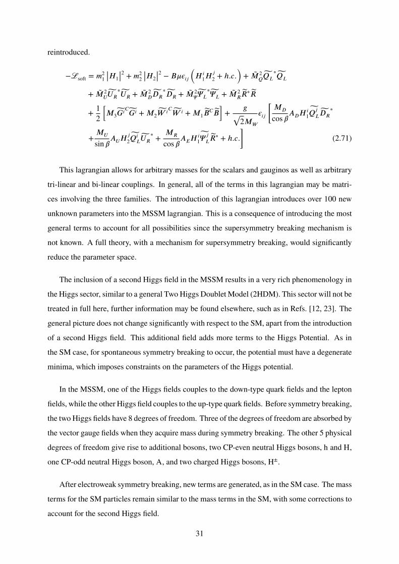
reintroduced.

−ℒsoft = 𝑚21 |𝐻1|

2 + 𝑚22 |𝐻2|

2 − 𝐵𝜇𝜖𝑖𝑗 (𝐻 𝑖1𝐻 𝑗

2 + ℎ.𝑐.) + ��2𝑄𝑄𝐿

∗𝑄𝐿

+ ��2𝑈𝑈𝑅

∗𝑈𝑅 + ��2𝐷𝐷𝑅

∗𝐷𝑅 + ��2𝛹𝛹𝐿

∗𝛹𝐿 + ��2𝑅𝑅∗𝑅

+ 12 [𝑀3𝐺𝑖𝐶𝐺𝑖 + 𝑀2𝑊 𝑖𝐶𝑊 𝑖 + 𝑀1𝐵𝐶𝐵] +

𝑔

√2𝑀𝑊

𝜖𝑖𝑗 [𝑀𝐷

cos 𝛽𝐴𝐷𝐻 𝑖

1𝑄𝑗𝐿𝐷𝑅

∗

+𝑀𝑈

sin 𝛽𝐴𝑈𝐻 𝑗

2𝑄𝑖𝐿𝑈𝑅

∗ +𝑀𝑅

cos 𝛽𝐴𝐸𝐻 𝑖

1𝛹 𝑗𝐿𝑅∗ + ℎ.𝑐.] (2.71)

This lagrangian allows for arbitrary masses for the scalars and gauginos as well as arbitrary

tri-linear and bi-linear couplings. In general, all of the terms in this lagrangian may be matri-

ces involving the three families. The introduction of this lagrangian introduces over 100 new

unknown parameters into the MSSM lagrangian. This is a consequence of introducing the most

general terms to account for all possibilities since the supersymmetry breaking mechanism is

not known. A full theory, with a mechanism for supersymmetry breaking, would significantly

reduce the parameter space.

The inclusion of a second Higgs field in the MSSM results in a very rich phenomenology in

the Higgs sector, similar to a general Two Higgs Doublet Model (2HDM). This sector will not be

treated in full here, further information may be found elsewhere, such as in Refs. [12, 23]. The

general picture does not change significantly with respect to the SM, apart from the introduction

of a second Higgs field. This additional field adds more terms to the Higgs Potential. As in

the SM case, for spontaneous symmetry breaking to occur, the potential must have a degenerate

minima, which imposes constraints on the parameters of the Higgs potential.

In the MSSM, one of the Higgs fields couples to the down-type quark fields and the lepton

fields, while the other Higgs field couples to the up-type quark fields. Before symmetry breaking,

the two Higgs fields have 8 degrees of freedom. Three of the degrees of freedom are absorbed by

the vector gauge fields when they acquire mass during symmetry breaking. The other 5 physical

degrees of freedom give rise to additional bosons, two CP-even neutral Higgs bosons, h and H,

one CP-odd neutral Higgs boson, A, and two charged Higgs bosons, H±.

After electroweak symmetry breaking, new terms are generated, as in the SM case. The mass

terms for the SM particles remain similar to the mass terms in the SM, with some corrections to

account for the second Higgs field.

31

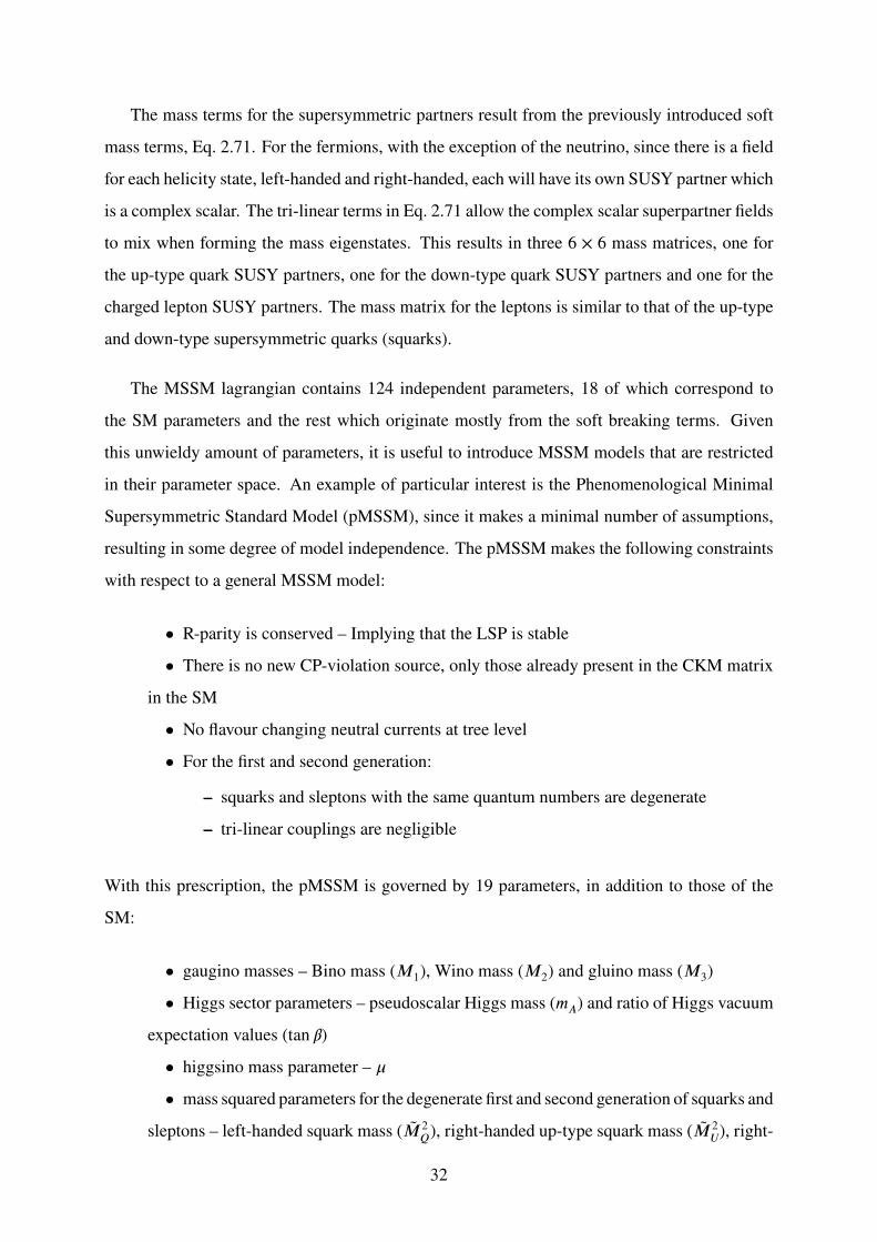
The mass terms for the supersymmetric partners result from the previously introduced soft

mass terms, Eq. 2.71. For the fermions, with the exception of the neutrino, since there is a field

for each helicity state, left-handed and right-handed, each will have its own SUSY partner which

is a complex scalar. The tri-linear terms in Eq. 2.71 allow the complex scalar superpartner fields

to mix when forming the mass eigenstates. This results in three 6 × 6 mass matrices, one for

the up-type quark SUSY partners, one for the down-type quark SUSY partners and one for the

charged lepton SUSY partners. The mass matrix for the leptons is similar to that of the up-type

and down-type supersymmetric quarks (squarks).

The MSSM lagrangian contains 124 independent parameters, 18 of which correspond to

the SM parameters and the rest which originate mostly from the soft breaking terms. Given

this unwieldy amount of parameters, it is useful to introduce MSSM models that are restricted

in their parameter space. An example of particular interest is the Phenomenological Minimal

Supersymmetric Standard Model (pMSSM), since it makes a minimal number of assumptions,

resulting in some degree of model independence. The pMSSM makes the following constraints

with respect to a general MSSM model:

• R-parity is conserved – Implying that the LSP is stable

• There is no new CP-violation source, only those already present in the CKM matrix

in the SM

• No flavour changing neutral currents at tree level

• For the first and second generation:

– squarks and sleptons with the same quantum numbers are degenerate

– tri-linear couplings are negligible

With this prescription, the pMSSM is governed by 19 parameters, in addition to those of the

SM:

• gaugino masses – Bino mass (𝑀1), Wino mass (𝑀2) and gluino mass (𝑀3)

• Higgs sector parameters – pseudoscalar Higgs mass (𝑚𝐴) and ratio of Higgs vacuum

expectation values (tan 𝛽)

• higgsino mass parameter – 𝜇

• mass squared parameters for the degenerate first and second generation of squarks and

sleptons – left-handed squark mass (��2𝑄), right-handed up-type squark mass (��2

𝑈), right-

32

handed down-type squark mass (��2𝐷), left-handed slepton mass (��2

𝛹) and right-handed

charged slepton mass (��2𝑅)

• corresponding mass squared parameters for the third generation of squarks and slep-

tons

• third generation 𝐴 parameters – top quark tri-linear coupling (𝐴t), bottom quark tri-

linear coupling (𝐴b) and tau lepton tri-linear coupling (𝐴τ)

So far, no experimental evidence consistent with SUSY has been observed. Consequently,

the results are expressed as limits, a summary of some of the results from the CMS collaboration

can be found in Fig. 2.7. The results are taken from [24] which compiles the results from several

CMS publications.

stop mass [GeV]

100 200 300 400 500 600 700 800

LSP

mas

s [G

eV]

0

100

200

300

400

500

600

700

W

= m

10χ∼

- m

t~m

t

= m

10χ∼

- m

t~m

= 8 TeVsCMS

1

0χ∼ / c 1

0χ∼ t →t~ production, t~-t

~

-1SUS-13-023 0-lep (2 body decays) 18.9 fb-1SUS-14-001 0-lep (2 body decays) 19.4 fb

-1SUS-13-011 1-lep (2 and 3 body decays) 19.5 fb-1SUS-14-015 1,2-lep (2 and 3 body decays) 19.5 fb

-1SUS-14-011 0-lep (Razor) + 1-lep (MVA) 19.5 fb-1SUS-14-011 0,1,2-lep (Razor) 19.3 fb

-1) 19.7 fb1

0χ∼ c →t~SUS-14-001 Monojet (

-1SUS-14-021 1-lep (4 body decays) 19.7 fb-1SUS-14-021 2-lep (4 body decays) 19.7 fb

ObservedExpected

t

= m

10χ∼

- m

t~m

(a) Stop

gluino mass [GeV]

600 800 1000 1200 1400 1600

LSP

mas

s [G

eV]

0

100

200

300

400

500

600

700

800

900

1000

m(g

luin

o) - m

(LSP) =

2 m

(top)

ICHEP 2014 = 8 TeVs

CMS Preliminary

1

0χ∼ t t →g~ production, g~-g~-1) 19.5 fbT+HTESUS-13-012 0-lep (

-1) 11.7 fbTαSUS-12-028 0-lep (-1SUS-14-011 0+1+2-lep (razor) 19.3 fb

-1) 19.3 fbφ∆SUS-13-007 1-lep (-1SUS-13-007 1-lep (LS) 19.3 fb

-1SUS-13-016 2-lep (OS+b) 19.7 fb-1SUS-13-013 2-lep (SS+b) 19.5 fb

-1SUS-13-002 (MultiLepton) 19.5 fb-1SUS-13-008 3-lep (3l+b) 19.5 fb

-1) 19.5 fb2

SUS-13-019 (MT-1SUS-12-024 b-jet 19.4 fb

(b) Gluino

squark mass [GeV]

400 600 800 1000 1200 1400

LSP

mas

s [G

eV]

0

100

200

300

400

500

600

700

800

900

ICHEP 2014 = 8 TeVs

CMS Preliminary

1

0χ∼ q →q~ production, q~-q~

-1) 19.5 fbTH+ T

SUS-13-012 (H

-1) 11.7 fbTαSUS-12-028 (

-1) 19.5 fbT2

SUS-13-019 (MObservedSUSYtheoryσObserved -1

Expected

q~one light

)c~, s~, d~

, u~ (R

q~ + L

q~

(c) Light Squark

neutralino mass = chargino mass [GeV]

100 200 300 400 500 600 700 800

LSP

mas

s [G

eV]

0

100

200

300

400

500

600

700

800

900

1

0χ∼

= m

1±χ∼m

Z+m1

0χ∼

= m

1±χ∼m

H+m1

0χ∼

= m

1±χ∼m

ICHEP 2014 = 8 TeVs

CMS Preliminary

production1

±χ∼-2

0χ∼

) 1

0χ∼)(W 1

0χ∼ (H → 1

±χ∼ 2

0χ∼

)1

0χ∼)(W 1

0χ∼ (Z → 1

±χ∼ 2

0χ∼

)τν∼τ∼ (1

±χ∼ 2

0χ∼

) )=1-l+l, BF(Rl~ (

1

±χ∼ 2

0χ∼

) )=0.5-l+l, BF(Ll~ (

1

±χ∼ 2

0χ∼

) )=1-l+l, BF(Ll~ (

1

-χ∼ 1

+χ∼

-1SUS-13-006 19.5 fb-1SUS-14-002 19.5 fb

1

0χ∼

= m

1±χ∼m

(d) Neutralino/Chargino

Figure 2.7: Selected SUSY results from the CMS collaboration. Figures taken from [24].

33

2.2.2 The case for Staus

The third generation of supersymmetric particles is normally viewed as the ideal candidate for

discovering SUSY. It is generally expected that some of these supersymmetric partners will

have lower masses than those of the first and second generations, making them more likely to be

produced at an accelerator. This lends itself to the fact that the highmasses of the third generation

SM particles make the mass mixing effects in the SUSY sector more pronounced with respect

to the first and second generations. To illustrate this effect, consider the mass matrix for the

charged leptons. Since the cross-family effects can often be neglected it is simpler to consider

each family on its own, effectively reducing the 6 × 6 mass matrix for the 3 families to a 2 × 2

mass matrix for each family. The mass matrix for the stau is represented in Eq. 2.72, the mass

matrices for the charged leptons of the other families are the same onlywith the adequate variable

substitutions. The off-diagonal terms in the mass matrices are proportional to the mass of the

lepton and lead directly to the above-mentioned mass mixing effects.

𝑀2τ =

⎛⎜⎜⎝

��2𝛹 + 𝑚2

τ + 𝐿τ 𝑚τ𝑋∗τ

𝑚τ𝑋τ ��2𝑅 + 𝑚2

τ + 𝑅τ

⎞⎟⎟⎠

(2.72)

With the following definitions:

𝑋τ = 𝐴τ + 𝜇∗ tan 𝛽 (2.73)

𝐿τ = (−12

+ sin2 𝜃𝑊) 𝑚2𝑍 cos 2𝛽 (2.74)

𝑅τ = − sin2 𝜃𝑊𝑚2𝑍 cos 2𝛽 (2.75)

The stau is often the lightest slepton within MSSM models, and frequently one of the light-

est supersymmetric particles, [25–28] and given that the current LHC results disfavour light

squarks and gluinos, the search for direct stau production becomes an interesting prospect. The

non-observation of such events can also provide useful insights since it would allow to set limits

on sectors of the MSSM which do not depend on the colour sector. Since the LSP is a natural

candidate for dark matter, the observed relic dark matter density poses constraints on the prop-

erties of the LSP. Furthermore, the coannihilation processes involving the LSP and the heavier

supersymmetric particles also affect the relic density [29]. In fact, a light stau, with a mass very

close to the LSP, can participate in these coannihilation processes and might be a key ingredient

for the observed relic dark matter density [29–32].

34

Recent results on the stau from the CMS collaboration can be found in [33]. Results from the

ATLAS collaboration can be found in [34, 35]. The best current limit on the stau mass comes

from the LEP experiments, with an upper limit on the mass close to 85GeV [36–39].

35

Chapter 3

Experimental Apparatus

3.1 The Large Hadron Collider

The LHC is the largest and highest energy particle accelerator in the world. It has a circumfer-

ence of 26.6 km and is installed in the tunnel built for LEP. The tunnel is located between 50m

and 175m below the surface. The LHC consists of two synchroton rings with counter rotating

particle beams, generally protons but lead-ions are also used. It was designed for a centre of

mass energy of 14TeV in proton-proton collisions with a peak luminosity of 1034 cm−2 s−1. An

in depth description of the LHC is available in [40].

3.1.1 Beam Injection

A schematic of the CERN accelerator complex can be seen in Figure 3.1. Protons for the ac-

celerators are produced by ionising hydrogen atoms, thus striping them of their electrons. The

protons subsequently undergo several acceleration steps prior to being delivered to the desired

experiment. For instance, for the LHC, protons are ionised and accelerated to an energy of

50MeV in the Linac2, which is a linear accelerator. The protons are then fed into a series of

synchrotons that sequentially increase the energy of the protons. The first is the Proton Synchro-

ton (PS) Booster, which increases the proton energy up to 1.4GeV. The second step in the chain

is the PS itself, after which the protons have achieved an energy of 25GeV. The next accelerator

37

is the SPS, after which the protons are injected into the LHC at an energy of 450GeV. Once

within the LHC the protons are accelerated up to the operating energy and are then made to

collide.

Figure 3.1: Schematic diagram of the CERN accelerator complex, not to scale. Taken from

[41].

Within the LHC, the particle beams are not continuous but are grouped into bunches. The

design parameters define that the bunches are separated by 25 ns, with each bunch containing

1011 protons. The bunch structure of the LHC beam is constrained by the filling scheme from

the lower energy accelerators. In theory, the beams could contain 3564 bunches, however to

allow for the ramp-up of the injection and kicker magnets and for the ejection kicker magnets

(abort gap) as well as other engineering constraints, only 2808 of those bunches are filled when

operating at the nominal bunch spacing. During the 2011 and 2012 data taking periods, the LHC

operated with a bunch spacing of 50 ns and consequently only 1380 bunches were filled.

38

3.1.2 Magnets

The magnets employed by the LHC to bend the trajectory of the particle beams are supercon-

ducting niobium-titanium coils, cooled to 1.9K with liquid helium. The dipoles are capable of

producing amagnetic field of 8.33T. Themagnets are divided into several categories, depending

on the configuration of the magnetic field, such as dipoles, quadrupoles, sextupoles and others.

The dipoles steer the beams and keep them in a nearly circular orbit, 1232 of these magnets are

used by the LHC. The quadrupoles focus the beams, 392 are located around the LHC ring. The

other magnets are used to perform more finely tuned adjustments to the beams. A full list of all

the magnets in the LHC, can be found in [42].

3.1.3 Luminosity

The quantity that measures the capability of a particle accelerator to produce interactions/events

is called the luminosity,ℒ, and it is the proportionality factor between the rate of events and the

cross section of those events, Eq. 3.1. The luminosity is a function of the beam parameters only

and can be written as Eq. 3.2 for a Gaussian beam, where 𝑁𝑏 is the beam intensity (number of

protons in a bunch), 𝑛𝑏 is the number of bunches, 𝑓Rev is the revolution frequency, 𝛾𝑟 = √1 − 𝑣2

𝑐2

is the relativistic gamma factor, 𝜖𝑛 is the normalised transverse beam emittance, 𝛽∗ is the beta

function (𝛽 (𝑠)) at the collision point and𝐹 is a geometric luminosity reduction due to the crossing

angle at the interaction point.

The beta function is the envelope around the trajectories of particles circulating in the lattice

composed by the quadrupoles, thus it is a design parameter of the accelerator. The normalised

beam emittance is an inherent property of the beam and characterises the quality of the beam. It

is a measure of the average spread of the particles in position and momentum phase space. The

width of the beam at a given point, 𝑠, in the orbit in the accelerator is given by Eq. 3.3. This

makes it clear that the luminosity is inversely proportional to the beam size at the interaction

39

point.

𝑑𝑁𝑑𝑡

= ℒ 𝜎 (3.1)

ℒ =𝑁2

𝑏 𝑛𝑏𝑓Rev𝛾𝑟

4𝜋𝜖𝑛𝛽∗ 𝐹 (3.2)

𝜎 (𝑠) = √𝜖𝑛𝛽 (𝑠) (3.3)

A related concept is that of integrated luminosity, which is the luminosity integrated over a

period of time, normally over a data taking period. The terms luminosity and integrated lumi-

nosity are sometimes used interchangeably and the same symbol is used for the two, care must

be taken to not confuse the two.

Given the probabilistic nature of processes under the domain of particle physics, in order to

study a certain process not only is it necessary for the process to occur and be recorded, but a

statistically significant number of such events must be recorded. The cross section of a certain

process quantifies the likelihood of that process to occur. Consequently, in general terms, in

order to obtain a significant number of recorded events:

• Common processes, which have higher cross sections, require lower luminosities in

order to be studied. However higher luminosities result in more recorded events which

imply improved statistical accuracy

• Rare processes, which have lower cross section, require higher luminosities in order

to be studied

High luminosities can be achieved through different ways, each with different trade-offs. For

instance, high luminosities can be achieved through a high number of particles, 𝑁𝑏 or 𝑛𝑏, or

through a small beam size, 𝜖𝑛 or 𝛽∗. Consider 𝛽∗, the beta function can be shown to have an

evolution according to Eq. 3.4 around the interaction point [43], where 𝑧 is the distance from

the interaction point along the beam direction. From Eq. 3.4 one can conclude that the smaller

the beam size at the interaction point (i.e. the smaller the 𝛽∗), the larger the beam size at some

distance from the interaction point. Thus, the smaller the beam size the larger the aperture of

the injection quadrupoles must be (as well as the quadrupole dimensions themselves) and the

larger the opening in the detector apparatus must be to allow the beam to enter the detector.

Requiring a larger opening in the detector apparatus reduces the coverage of the detector and

consequently also affects the performance of the detector. Thus, despite requiring the smallest

40

𝛽∗ possible to obtain the smallest beam width possible and consequently the largest luminosity

possible, the choice of the 𝛽∗ value is a compromise between the smallest value possible which

still allows for reasonable dimensions of the injection quadrupoles and resulting an as small as

possible opening at the ends of the detector apparatus.

𝛽 (𝑧) = 𝛽∗ + 𝑧2

𝛽∗ (3.4)

3.1.4 Pileup

A consequence of a high beam intensity (𝑁𝑏) is that, in each bunch crossing, more than one

proton-proton collision may occur. These “extra” interactions make the analysis of a process of

interest challenging because they contribute extra particles to a particular bunch crossing and

consequently to the measurement of the event. This effect of additional interactions is usually

referred to as in-time Pile-up (PU), often referred to only as PU.

With the extremely small bunch spacing employed by the LHC, in particular with the 25 ns

bunch spacing, the particles resulting from an interaction in a first bunch crossing do not have

time to exit the detector before a second bunch crossing occurs. Consequently, it is possible for

the detector to be measuring particles from different bunch crossings at a given instant in time.

This leads to a distinct kind of PU than that described above. To distinguish between the two,

the terms in-time PU and out-of-time PU are used.

A similar concept to that of PU is that of the underlying event. In a given interaction, two

protons are made to collide, however the particles that actually collide are individual partons

from each proton, the so-called hard interaction. The remaining partons from each proton go on

to create showers of particles, normally close to the beam line, which constitute the so-called

underlying event. These showers also contribute additional particles to the measurement (with

respect to the hard interaction), just like for the PU. It should also be mentioned that in a single

bunch crossing it is possible for several pairs of protons to collide, resulting in multiple interac-

tions for each bunch crossing, further compounding the issues above.

41

3.2 Compact Muon Solenoid

The CMS detector is located at one of the four interaction points around the LHC and it is about

100m beneath the surface at the foothills of the Jura mountains in Cessy, France. It is a general

purpose detector and covers almost the full solid angle around the interaction point. It is 21.6m

long and has a diameter of 14.6m and weighs 14 000 t. A diagram of the detector can be seen

in Fig. 3.2.

C ompac t Muon S olenoid

Figure 3.2: Schematic diagram of the CMS detector. Taken from [44].

The central feature of the CMS apparatus is a superconducting solenoid of 6m internal di-

ameter, providing a magnetic field of 3.8T. Within the superconducting solenoid volume are a

silicon pixel and strip tracker, a lead tungstate crystal Electromagnetic Calorimeter (ECAL), and

a brass and scintillator Hadronic Calorimeter (HCAL), each composed of a barrel and two end-

cap sections. Muons are measured in gas-ionisation detectors embedded in the steel flux-return

yoke outside the solenoid. A more detailed description of the CMS detector, together with a def-

inition of the coordinate system used and the relevant kinematic variables, can be found in [45,

42

46]. The rapidity coverage of the CMS detector ranges between 2.4 and 5.2, depending upon

the subdetector system considered.

3.2.1 Coordinate System

As is required, the CMS experiment uses a right-handed coordinate system. The origin of the

coordinate system is defined as the nominal interaction point, with the 𝑥 axis pointing to the

centre of the LHC, the 𝑦 axis perpendicular to the LHC plane pointing up and the 𝑧 axis pointing

in the anti-clockwise beam direction. The polar angle, 𝜃, is measured from the positive 𝑧 axis

and the azimuthal angle, 𝛷, is measured from the positive 𝑥 axis in the 𝑥𝑦 plane.

3.2.2 Tracker

The CMS tracker is designed to provide a measurement of the position of charged particles

when they cross the silicon detectors within the volume of the tracker. These measurements

allow to reconstruct the trajectory of the charged particles, further detailed in chapter 4. The

reconstruction of the charged particle tracks has an essential role in the reconstruction of charged

particles (electrons, muons, taus, hadrons and jets) as well as the determination of the interaction

vertices. The tracks are also fundamental for the identification of b-jets, in particular through

the evidence of a displaced vertex.

The functioning principle of silicon detectors relies on a reverse biased diode, creating a

depletion zone with an electric field between the contacts of the diode. When a charged particle

traverses the depletion zone, free electrons and holes are produced through ionisation. The

electric field in the depletion zone causes the electrons and holes to travel in opposite directions,

to the contacts of the diode, resulting in an electrical pulse that can be measured. By covering

an area with several such detectors, it is possible to identify where a charged particle traversed.

The tracker is completelymade of silicon detectors and is the largest silicon tracker ever built.

Two types of silicon detectors compose the tracker, pixel detectors and strip detectors, used in

each tracker subsystem: the Silicon Pixel Detector and the Silicon Strip Detector, respectively.

Fig. 3.3 illustrates a schematic view of the CMS tracker in an 𝑟-𝑧 slice, with the different detector

43

subsystems identified. The nominal resolution of the tracker system on the momentum of a

charged particle is typically 0.7 (5.0) % at 1 (1000) GeV in the central region and on the impact

parameter is typically 10 μm for high momentum tracks. An in depth description of the tracker

system and a description of its performance can be found in [46, 47].

Figure 3.3: Schematic diagram of the CMS tracker in an 𝑟-𝑧 slice. Single lines represent layers

of modules equipped with one sensor, double lines indicate layers with back-to-back modules.

Taken from [47].

Silicon Pixel Detector

The silicon pixel detector has 66 million active elements over a surface area of about 1m2. It

covers a region from 4 cm to 15 cm in radius and 49 cm on each side of the interaction point. The

detector consists of several layers, three in the barrel region and two on each side in the endcap

region. The detector is designed to determine three very high precision three-dimensional points

for each track. This is achieved through the use of active elements of n-in-n pixels with dimen-

sions of 100 μm×150 μm. The detector further exploits the presence of the 3.8Tmagnetic field,

for barrel and endcap, coupled with a geometric arrangement, for the endcap, to achieve sub-

pixel resolution of the measurement of where a charged particle has passed through the sensor.

Considering the particle flux at nominal luminosity, the pixel detectors are expected to have an

average occupancy per LHC crossing of 0.01%.

44

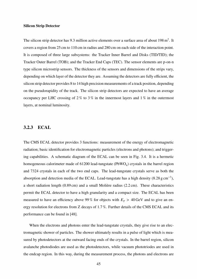
Silicon Strip Detector

The silicon strip detector has 9.3 million active elements over a surface area of about 198m2. It

covers a region from 25 cm to 110 cm in radius and 280 cm on each side of the interaction point.

It is composed of three large subsystems: the Tracker Inner Barrel and Disks (TID/TID); the

Tracker Outer Barrel (TOB); and the Tracker End Caps (TEC). The sensor elements are p-on-n

type silicon microstrip sensors. The thickness of the sensors and dimensions of the strips vary,

depending on which layer of the detector they are. Assuming the detectors are fully efficient, the

silicon strip detector provides 8 to 14 high precisionmeasurements of a track position, depending

on the pseudorapidity of the track. The silicon strip detectors are expected to have an average

occupancy per LHC crossing of 2% to 3% in the innermost layers and 1% in the outermost

layers, at nominal luminosity.

3.2.3 ECAL

The CMS ECAL detector provides 3 functions: measurement of the energy of electromagnetic

radiation; basic identification for electromagnetic particles (electrons and photons); and trigger-

ing capabilities. A schematic diagram of the ECAL can be seen in Fig. 3.4. It is a hermetic

homogeneous calorimeter made of 61200 lead-tungstate (PbWO4) crystals in the barrel region

and 7324 crystals in each of the two end caps. The lead-tungstate crystals serve as both the

absorption and detection media of the ECAL. Lead-tungstate has a high density (8.28 g cm−3),

a short radiation length (0.89 cm) and a small Molière radius (2.2 cm). These characteristics

permit the ECAL detector to have a high granularity and a compact size. The ECAL has been

measured to have an efficiency above 99% for objects with 𝐸𝑇 > 40GeV and to give an en-

ergy resolution for electrons from Z decays of 1.7%. Further details of the CMS ECAL and its

performance can be found in [48].

When the electrons and photons enter the lead-tungstate crystals, they give rise to an elec-

tromagnetic shower of particles. The shower ultimately results in a pulse of light which is mea-

sured by photodetectors at the outward facing ends of the crystals. In the barrel region, silicon

avalanche photodiodes are used as the photodetectors, while vacuum phototriodes are used in

the endcap region. In this way, during the measurement process, the photons and electrons are

45

Figure 3.4: Schematic diagram of the CMS ECAL. Taken from [49].

absorbed by the detector.

The barrel part of the ECAL is subdivided into 360 crystals in 𝛷 and 2 × 85 in 𝜂 and covers

the range |𝜂| < 1.497. The crystals are mounted at a small angle with respect to the direction to

the nominal interaction point in order to avoid particles passing through cracks in the detector.

The crystal dimensions are roughly 22 × 22mm2 at the front face and 26 × 26mm2 at the rear

face, with a length of 230mm, corresponding to about 25.8 radiation lengths.

The end caps cover the range 1.497 < |𝜂| < 3.0, with the crystals arranged in a rectan-

gular grid in (𝑥, 𝑦). To avoid cracks in the detector where particles could escape the crystals

point at a focus 1300mm beyond the nominal interaction point, thus being mounted at a small

angle to the interaction point, similarly to the barrel region. The crystals have dimensions of

28.62 × 28.62mm2 at the front face and 30 × 30mm2 at the rear face, with a length of 220mm,

corresponding to about 24.7 radiation lengths.

Not that the ECAL crystals have dimensions compatible with the Molière radius of the mate-

rial they are composed of, consequently the electromagnetic showers produced when a particle

interacts in the crystals will leak into adjoining crystals. Consequently, the energy of the par-

ticles is measured as clusters of crystals and the clusters can further be used to reconstruct the

position where the shower began, i.e. where the particle interacted.

46

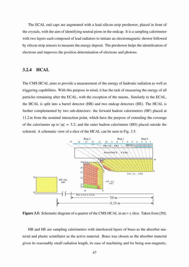
The ECAL end caps are augmented with a lead-silicon-strip preshower, placed in front of

the crystals, with the aim of identifying neutral pions in the endcap. It is a sampling calorimeter

with two layers each composed of lead radiators to initiate an electromagnetic shower followed

by silicon strip sensors to measure the energy deposit. The preshower helps the identification of

electrons and improves the position determination of electrons and photons.

3.2.4 HCAL

The CMS HCAL aims to provide a measurement of the energy of hadronic radiation as well as

triggering capabilities. With this purpose in mind, it has the task of measuring the energy of all

particles remaining after the ECAL, with the exception of the muons. Similarly to the ECAL,

the HCAL is split into a barrel detector (HB) and two endcap detectors (HE). The HCAL is

further complemented by two sub-detectors: the forward hadron calorimeters (HF) placed at

11.2m from the nominal interaction point, which have the purpose of extending the coverage

of the calorimeter up to |𝜂| = 5.2; and the outer hadron calorimeter (HO) placed outside the

solenoid. A schematic view of a slice of the HCAL can be seen in Fig. 3.5.

Figure 3.5: Schematic diagram of a quarter of the CMS HCAL in an 𝑟-𝑧 slice. Taken from [50].

HB and HE are sampling calorimeters with interleaved layers of brass as the absorber ma-

terial and plastic scintillator as the active material. Brass was chosen as the absorber material

given its reasonably small radiation length, its ease of machining and for being non-magnetic,

47

since it is located within the CMS solenoid. The plastic scintillator is an ideal choice for the ac-

tive material since it allows to maximise the amount of absorber material before the solenoid. To

catch possible energy leakage from the HB, layers of scintillators are placed outside the solenoid,

constituting the HO. A more in depth description of the HCAL can be found in [46, 50].

The HB covers the range |𝜂| < 1.3. It is built of 18 wedges, each covering 20° in the

azimuthal angle, with each divided into four 5° sectors. Each half is split into 16 towers in

𝜂. The overall design gives an effective segmentation of 0.087 × 0.087 in the 𝜂 × 𝛷 space. Its

thickness corresponds to 5.8 hadronic interaction lengths at 𝜂 = 0 and goes up to 10 at |𝜂| = 1.2.

The HO catches the energy leakage from the HB and is placed in the inner layer of the

return yoke. It has two scintillator layers in the innermost region (close to 𝜂 = 0) and a single

layer in the rest of the barrel region. This subdetector extends the coverage of the HCAL by

effectively increasing the radiation lengths of the detector to over 10 hadronic radiation lengths.

Geometrically, it is constrained by the muon system and closely follows its geometry, having 12

identical sectors in 𝛷. 95% of all hadrons above 100GeV deposit energy in the HO.

The HE covers the range 1.3 < |𝜂| < 3.0. It is made of brass disks, interleaved with scintil-

lator wedges which cover 20° in the azimuthal angle. Each endcap is split into 14 towers in 𝜂.

The outermost towers (smaller 𝜂) have a segmentation of 5°, while the innermost towers have a

segmentation of 10°.

The HF covers the range 3.0 < |𝜂| < 5.2. One of the main purposes of this detector is the

real time measurement of the luminosity delivered to CMS. The HF consists of a steel absorber

structure of 5mm thick plates alternatingwith quartz fibres as the active elements which generate

a signal through the Cherenkov effect. The fibres are parallel to the beam direction and for the

measurement the fibres channel the Cherenkov light to photomultipliers.

3.2.5 Superconducting Solenoid

The CMS superconducting solenoid is 12.5m long and has a diameter of 6m. It is designed to

produce a 4T magnetic field, storing 2.6GJ of energy when at full current. The magnetic flux

is returned through an iron return yoke, which envelopes the CMS detector. The return yoke

weights 10 000 t and is divided into 5 wheels and 2 end caps, with each endcap being divided into

48

3 disks. The yoke’s purpose is to increase the homogeneity of the magnetic field in the tracker

volume and reduce the stray field by returning the magnetic flux of the solenoid. The return

yoke also serves as structural support for the whole CMS detector. The CMS Collaboration has

decided to operate the superconducting solenoid at 3.8T, instead of the nominal 4T, until a more

in depth understanding of the ageing of the solenoid has been obtained [51].

In order to accurately reconstruct the tracks of charged particles and in order for the simu-

lated events to match the observed data as close as possible, a detailed map of the magnetic field

is required. The field within the solenoid was mapped with specialised Hall effect sensors prior

to the assembly of the CMS detector [52]. Further measurements during the assembly of the

detector confirmed the validity of the previous measurements in the presence of the detectors

within the solenoid. The field outside the solenoid, within the return yoke, is affected by the

magnetic environment surrounding the CMS detector. Consequently, dedicated runs with cos-

mic muons were employed to map the magnetic field in this region [51]. In this way, the CMS

magnetic field is mapped, in the central region to a precision better than 0.1% and in the yoke

to a precision of 3% to 8%.

3.2.6 Muon Chambers

Themuon system in CMS has threemain functions: muon identification; muonmomentummea-

surement; and triggering. The muon system employs three types of gaseous particle detectors:

drift tubes (DT); cathode strip chambers (CSC); and resistive plate chambers (RPC). The choice

of which technologies were used is driven by the different radiation environments and the areas

to be covered. In the barrel region, where the muon rates are low, DTs are used. In the endcap

region, where the muon rates are high, CSCs are used. Both DTs and CSCs have the capability

to trigger on the transverse momentum of the muons with good efficiency and high background

rejection. However, due to the uncertainty on the background rates and the ability to measure

the correct beam crossing time when the LHC reaches full luminosity a complementary system,

consisting of RPCs was added to both the barrel and end caps. This addition stems from the

fact that the RPCs provide a faster signal at the cost of a coarser resolution with respect to the

DTs and CSCs. A schematic diagram of the CMS muon detectors and their layout can be seen

in Fig. 3.6. The DTs and CSCs provide CMS with muon track segments for triggering with an

49

efficiency above 96% and correctly identify the bunch crossing in over 99.5% of the cases. An

in depth analysis of the performance of the muon system as well as a more in depth description

of the detector can be found in [53].

0 2 4 6 8 10 12 z (m)

R (m

)

1

0

2

3

4

5

6

7

8

1 3 5 7 95.0

4.0

3.0

2.52.42.32.22.12.0

1.9

1.8

1.7

1.6

1.5

1.4

1.3

1.2

1.00.9 1.10.80.70.60.50.40.30.20.140.4°44.3° 36.8°48.4°52.8°57.5°62.5°67.7°73.1°78.6°84.3°

0.77°

2.1°

5.7°

9.4°10.4°11.5°12.6°14.0°15.4°

17.0°

18.8°

20.7°

22.8°

25.2°

27.7°

30.5°

33.5°

!°η

!°η

ME4

/1

ME3

/1

ME2

/1

ME1

/2

ME1

/1

ME2

/2

ME3

/2

ME1

/3

RE3

/3

RE1

/3R

E1/2

MB1

MB2

MB3

MB4

Wheel 0 Wheel 1

RB1

RB2

RB3

RB4

HCAL

ECAL

Solenoid magnet

Silicon tracker

Steel

DTsCSCsRPCs

RE2

/2

Wheel 2

RE2

/3

RE3

/2

11

Figure 3.6: Schematic diagram of a quarter of the CMS detector in an 𝑟-𝑧 slice. The interaction

point is at the lower left corner. The steel return yoke is shown in dark grey. The DTs are

illustrated in light orange, the CSCs are illustrated in green and the RPCs are illustrated in blue.

The different layers of the DTs are labelled MB, the CSC layers are labelled ME and the RPC

layers are labelled RB and RE, depending on whether it is a barrel or endcap layer, respectively.

Taken from [53].

3.2.7 Trigger

With the nominal LHC bunch spacing, it is expected to have a collision every 25 ns, correspond-

ing to a rate of 40MHz. The size of an event at CMS is 𝒪(1) MB, consequently storing all

events would require to store 40TB of data every second. Storing such an amount of data is

clearly a gargantuan task. With this in mind, a reduction on the rate of events to be kept and

50

analysed must be performed, ideally by discarding the uninteresting events and keeping the in-

teresting ones. This is the task of the trigger system, thus corresponding to the first step of the

physics event selection and analysis. The interesting events are defined as those events where

it is expected to find evidence of new physics or events where more precise measurements are

desired, which correspond to events within specific ranges. In general, it is expected that new

physics will be manifested by new particles, with higher masses, thus corresponding to events

containing objects with higher transverse momentum. Consequently, the remaining events are

considered uninteresting and are discarded.

In CMS the trigger system is split into two steps, the Level–1 (L1) trigger and the High-

Level Trigger (HLT), with the L1 feeding directly into the HLT. The L1 trigger consists of

custom designed, largely programmable, electronics, which are located on the detector and in

its vicinity. The HLT trigger is a software system implemented in a computing farm. The HLT

has the task of reducing the event rate from around 100 kHz, originating from the L1 trigger, to

less than 1 kHz before storage. More in depth descriptions of the trigger systems can be found

in [54–56].

L1

The L1 trigger only uses coarse data from the calorimeters and muon system, while the full

granularity data is stored on the detector front-end electronics waiting for the L1 decision. The

allowed L1 trigger latency, between a given bunch crossing and the distribution of the trigger

decision to the detector front-end electronics, is 3.2 μs. The mismatch between the trigger la-

tency (3.2 μs) and the bunch crossing rate (25 ns) is managed through buffers on the front-end

electronics, which hold the information until a decision by the L1 trigger has been reached. The

L1 trigger is implemented pipelined logic to allow for the necesary throughput to reach a deci-

sion for each bunch crossing. The trigger decision is based on local, regional and global trigger

components. A flow chart of the trigger architecture is displayed in Fig. 3.7.

The ECAL and HCAL cells are combined to form so-called trigger towers. Trigger primi-

tives are generated by calculating the transverse energy of each tower. A regional calorimeter

trigger then determines electron, photon and jet candidates and information relevant for muon

and tau identification, on a regional level. The global calorimeter trigger calculates the total

51

Figure 3.7: Flow chart of the CMS L1 trigger. Taken from [57].

transverse energy and the Missing Transverse Energy (MET), also providing information about

the jets and the highest ranking trigger candidates.

All the types of muon detectors take part in the muon trigger. The DT chambers provide track

segments in the 𝜙 projection and hit pattern in 𝜂, while the CSC determine three-dimensional

track segments. The track finders in the DT and CSC calculate the transverse momentum, loca-

tion and quality of a track segment. The RPCs use regional hit patterns to provide an independent

measurement. The global muon trigger receives up to 4 candidate muons from each subsystem in

conjunction with isolation information from the regional calorimeter trigger. The global muon

trigger selects a maximum of four muon trigger candidates and determines their momentum,

charge, position and quality.

The trigger objects identified by the global calorimeter trigger and the global muon trigger

are forwarded to the global trigger. The global trigger makes the decision to accept or reject an

event based on the results of algorithms which for example apply thresholds on the momentum

of the objects or require a certain number of object to be present. The decision is then distributed

back to the detectors so the full event information, with a size of 𝒪 (1MB), can be read out to

the HLT trigger.

52

HLT

The HLT is implemented as a set of software filters that runs in a processor farm, thus being

fully parallelized. The HLT processes all events accepted by the L1 trigger, i.e. it is seeded by

the L1 trigger. The selection of events is optimised by rejecting events early, i.e. as soon as there

is enough information to decide to not keep it. The reconstruction algorithms used are generally

the same as those used for offline analysis, but to optimise for speed some features are sometimes

only partially reconstructed. Such as only a restricted region of the detector is reconstructed or

a limited set of information from the physics objects is retrieved. The HLT selection algorithms

are organised in paths, an event is accepted by the HLT if it is accepted by any path.

3.2.8 DAQ

The CMS trigger and Data Acquisition (DAQ) system is designed to collect and analyse the

detector information at the LHC frequency of 40MHz. The DAQ system must not only sustain

a rate of 100 kHz from the L1 trigger, at a total bandwidth of 100GB s−1 from approximately

650 different sources (about 200MB s−1 each), but it must also provide the computing power

for the HLT to perform its task of further reducing the event rate to less than 1 kHz. Data is

collected in so-called runs, during which the DAQ parameters do not change.

3.2.9 DQM

The Data Quality Monitoring (DQM) system continuously monitors the quality of the data. A

sample of the recorded events are reconstructed, in particular calibration events, from which

a large set of quantities are collected in histograms and compared between runs and reference

values by both automated processes and through human intervention. If significant deviations

are observed, the corresponding luminosity sections (lumisections) are marked as bad. CMS

has defined a lumisection as a fixed period of time, set to 218 LHC orbits, which roughly corre-

sponds to 23.3 s. The information on the bad lumisections is combined with the detector status

information to produce a curated list of certified runs and lumisections. In this way, only data

that is known to be good is included in the physics analyses.

53

3.2.10 Luminosity and Pileup Measurement

In CMS two detectors are exploited to measure the luminosity, the forward hadronic calorimeter

and the silicon pixel detector [58]. The forward hadronic calorimeter features a dedicated high

rate acquisition system, the HF luminosity transmitter, which is independent from the central

DAQ and provides a real-time luminosity measurement. It is capable of determining the lu-

minosity with 1% statistical uncertainty in 1 s, however it is subject to calibration drift and is

non-linear with pileup. Thus, the preferred method for estimating the luminosity is using the

silicon pixel detector.

The silicon pixel detector is characterized by a very low occupancy, below 0.1%, and con-

sequently is stable throughout data taking. The luminosity is estimated using the Pixel Cluster

Counting method. The number of pixel clusters ocurring on average in an event (⟨𝑛⟩), triggered

by requiring only two bunches to cross at the interaction point, is used to estimate the luminos-

ity, Eq. 3.5, where 𝜈 is the beam revolution frequency and 𝜎vis is the visible cross section. The

visible cross section is measured in dedicated “Van der Meer” runs.

ℒ =𝜈 ⟨𝑛⟩𝜎vis

(3.5)

The luminosity of each bunch crossing, Eq. 3.5, multiplied by the total inelastic cross section

results in the number of interactions for the considered bunch crossing. Performing this proce-

dure for all the bunch crossings in data results in the distribution of the number of interactions

in data, also referred to as the PU distribution.

54

Chapter 4

Software Framework

CMS has put in place a common, generic event processing framework, which is also a model

for data storage for the HLT, event reconstruction and analysis. The event processing code is

written in C++ and the processing jobs are configured in Python. The job results are stored to

disk with the ROOT framework. It is called the cmssw framework. An in depth description can

be found in [59].

4.1 Simulation

An important part of any high energy physics analysis resides in the simulation of events, al-

lowing to compare the experimental results with the theoretical predictions. In practical terms,

a simulation provides simulated events which can be treated as if they were real events, through

the reconstruction and analysis steps. The simulated events are generally produced through the

Monte Carlo (MC) method, with repeated random sampling of the theoretical distributions; for

this reason as a shorthand the simulations are often referred to only as MC. MC events are also

used for studying and optimising the selection criteria prior to seeing the experimental results.

Simulation generally consists of three steps: the simulation of the proton–proton interaction;

the propagation of the final state particles through the detector volume; and the response of the

sensors to the particles. The PU is modelled bymixing simulated minimum-bias events on top of

the simulated hard interaction before reconstruction of the event. Technically the simulation is

55

performed within the cmssw framework, however some of the simulation softwares that perform

the initial step of the simulation, called generators, are run as standalone programs and the output

is subsequently fed into cmssw.

4.1.1 Event Generation

The interaction of two colliding protons is simulated with event generators, typically using the

MC method. There exist general purpose event generators, such as pythia [60] and herwig

[61], which simulate a variety of physical processes and also the parton shower and hadroni-

sation. There are also specialised generators which focus on specific objectives and can be

interfaced with other generators, such as the general purpose ones, in order to obtain the final

physical states, i.e. the event after hadronisation process. An example of a specialised generator

is tauola [62], which simulates decays of only the τ lepton, with the specificity of including its

polarisation.

MadGraph [63] is another commonly used generator, it is designed to generate matrix el-

ements. The matrix element squared is an essential component for computing the cross section

of a given physics process [64]. Once the matrix elements have been generated, MadGraph

can evaluate the cross section or decay width of the associated process. Within the MadGraph

framework, MadEvent can subsequently be used to generate events. The generated events must

then be processed with any program capable of simulating the parton shower and hadronisation,

such as pythia or herwig.

4.1.2 Detector Simulation

The evolution of the event through time and space after hadronisation as well as the interaction of

the particles with matter constitute the detector simulation. Particles are propagated through the

detector volumes and new particles are produced in the interactions with the detector material.

The CMS detector simulation is performed with the Geant4 [65] toolkit, which is written in

C++ and integrated within cmssw. The Geant4 toolkit is the tool that effectively propagates

the particles in time and space, through the detector volumes, and simulates the interaction of

these particles with matter, which results in simulated energy deposits in the detector volumes.

56

The energy deposits in the detector volumes are converted to digitised signals using algorithms

based on the observed detector behaviour. At this point, the digitised signals of the simulated

event are similar to those of a real event and can be treated as any other event with the cmssw

event reconstruction and analysis chain.

4.1.3 Fast Simulation

The above described simulation approach is commonly referred to as FullSim, since it consti-

tutes a full simulation of the whole physics and detector chain. It is a very time and resource

intensive process. Another approach is the so-called fast simulation, FastSim, which performs

about 100 times faster than the FullSim. In the FastSim approach, the events are generated with

the event generators, like for the FullSim. The particles are then propagated through the detec-

tor volume. The material effects and the response of the detectors to the particles are obtained

through parameterisation at the hit level. The results can then be treated as any other event with

the cmssw event reconstruction and analysis chain. A more in depth description of the CMS

FastSim can be found in [66]. For this work, the FastSim approach is only used to process the

signal samples, with FullSim being used to process all background samples.

4.1.4 Pileup Modelling

The PU interactions are modelled by mixing simulated minimum-bias events on top of the sim-

ulated hard-interaction events. Since the simulation efforts must start prior to all the data being

collected, the distribution of the number of PU interactions in data is unknown. Therefore, the

simulated events are generated with an assumed PU distribution and the events are re-weighted

at the analysis time such that the PU distributions between data and simulation agree.

4.2 Event Reconstruction

Raw data from the CMS detector is, in essence, a collection of voltage readings from the various

elements of the detector at the time of the event. However, to perform meaningful physical anal-

57

yses, it is preferable to work in terms of the particles that generated the observed signals. Thus,

sets of algorithms, made to reconstruct the particles from the raw data, are implemented. These

reconstructed particles form the so-called physics objects. The CMS Physics Object Groups

(POGs) define a set of recommendations so that physics analysis can have a common set of

definitions and parameters when using the above-mentioned physics objects, so-called working

points.

4.2.1 Tracking

The tracking reconstruction has the purpose of reconstructing the trajectories of the charged

particles from the energy deposits in the tracker detector. For the trajectories of muons, the

energy deposits in the muon chambers, also referred to as the hits in the muon chambers, are

also used. Given the presence of the magnetic field, aligned with the 𝑧 axis, the trajectories of

the charged particles are bent, in the transverse plane (the 𝑥𝑦 plane), and the charged particles,

free from any other interactions, move along helices. With the reconstructed trajectories it is

possible to measure the curvature of the trajectory. The curvature of the trajectory of the particle

is an important measure since it relates directly with the momentum of the particle. The basic

principle for this relation stems from equating the centripetal force with the magnetic force,

Eq. 4.1, which results in an equation relating the momentum with the radius of the curvature of

the trajectory of a particle, Eq. 4.2.

𝐹𝐶 ≡ 𝑚𝑣2

𝑟= 𝑞𝑣𝐵 ≡ 𝐹𝐵 (4.1)

𝑝 ≡ 𝑚𝑣 = 𝑞𝑟𝐵 (4.2)

Thus, exploiting the tracking with the magnetic field, which bends the particles in the transverse

plane, permits to measure the momentum of the particles in the transverse plane, the so-called

transverse momentum, 𝑝𝑇. Using simple trigonometry it is possible to relate the 𝑝𝑇 with the

total momentum using the angle 𝜃 of the trajectory, which is obtained from the tracking as well,

Eq. 4.3.

𝑝 =𝑝𝑇

sin 𝜃(4.3)

The large multiplicity of particles expected to be created in each event poses a challenge

for the tracking algorithm. The hits associated to each track must be found and fitted in order

58

to obtain the track parameters. For this purpose CMS uses the so-called combinatorial track

finder (CTF) algorithm. The CTF algorithm proceeds through three stages: track seeding; track

finding; and track fitting. The track candidates are seeded from the hits in the pixel detector. The

track finding stage is based on Kalman filters, where the trajectory is extrapolated to the next

layer and compatible hits are associated to the track. The Kalman filter proceeds to update the

track parameters with the new hit. In the final stage, the tracks are refitted with a Kalman filter

and a second fitter (smoother) running from the exterior towards the beam line. More detailed

descriptions can be found in [67, 68]. The muon tracking exploits the hits in the muon detector,

where it is unlikely for particles that are not muons to reach. Conversely, the electron tracking

has to handle not only the electron tracks, but tracks from all other charged particles, resulting in

a much more challenging reconstruction environment. The CMS tracking is designed to provide

an efficiency above 99% for single muons with a transverse momentum above 1GeV, for more

details see [69].

4.2.2 Primary Vertices

The particle tracks, reconstructed as explained in the previous section, allow the reconstruction

of the position of the interaction. In the presence of PU, a single event may contain multiple

interaction points. In general, a single interaction per event is considered the Primary Vertex

(PV). The vertex reconstruction can be separated into two steps, the clustering of the tracks in

order to find the best partition of the tracks and the fitting of the set of tracks to the vertex.

The tracks are clustered using the so-called Deterministic Annealing clustering of tracks [70].

The reconstructed vertex is required to have a 𝑧 position within the nominal detector centre

(|𝑧| < 24 cm) and a radial position within the beam-spot (|d 0| < 2 cm). The reconstructed

vertices are also required to have more than four degrees of freedom in the vertex fit. From the

set of vertices passing these criteria, the vertex with the highest ∑tracks 𝑝2𝑇 is chosen as the PV.

More details can be found in [71, 72]

59

4.2.3 Particle Flow

The Particle Flow (PF) algorithm reconstructs and identifies each individual particle in an event

by using an optimised combination of information from the various elements of the CMS de-

tector. One advantage of using the PF approach to the object identification is that it provides a

consistent set of reconstructed particles for each event. The main ingredients for the PF algo-

rithm, which are provided by the CMS detector, are an efficient and pure track reconstruction

with a small material budget in front of the calorimeters, a good calorimeter granularity, a large

magnetic field and a good separation between charged and neutral hadrons. A more detailed

description of the PF algorithm can be found in [73, 74]. The algorithm can be described in

the following simplified picture. Muons are identified in a first step, since they are the only

measured objects reaching the muon chambers, and their tracks are removed from consideration

for the subsequent steps. Tracks are extrapolated to the calorimeters and if they fall within the

boundaries of one or several clusters, the clusters are associated to the track. This set consti-

tutes the charged hadron candidates and the base objects are not considered for the remainder

of the algorithm. A specific track reconstruction is used for the electrons, given the emission of

Bremsstrahlung photons. A dedicated procedure properly associates the energy deposits from

Bremsstrahlung photons with the electron track. Once all the tracks have been processed, the

remaining deposits are considered photons, in the case of the ECAL, and neutral hadrons, in the

case of the HCAL. Once each particle has had its energy deposits associated, its nature can be

evaluated and the information from the subdetectors combined to determine its energy.

The energy of photons is directly obtained from the ECAL measurement, corrected for zero-

suppression effects. The energy of electrons is determined from a combination of the electron

momentum at the primary interaction vertex as determined by the tracker, the energy of the

corresponding ECAL cluster, and the energy sum of all Bremsstrahlung photons spatially com-

patible with originating from the electron track. The energy of muons is obtained from the

curvature of the corresponding track. The energy of charged hadrons is determined from a com-

bination of their momentum measured in the tracker and the matching ECAL and HCAL energy

deposits, corrected for zero-suppression effects and for the response function of the calorimeters

to hadronic showers. Finally, the energy of neutral hadrons is obtained from the corresponding

corrected ECAL and HCAL energy. The four-momenta of individual particles can subsequently

be used to cluster jets, to compute the MET, and to reconstruct the hadronic decays of the τ

60

lepton. The list of individual particles is also used to measure the isolation parameter of the

particles.

4.2.4 Jets

Quarks and gluons fragment and hadronise almost immediately after being produced, leading

to a collimated spray of energetic hadrons, called a jet. Consequently, jets are the experimental

signature of quarks and gluons produced in a collision. Thus, jets are reconstructed by clustering

the set of reconstructed particles into groups. Several algorithms have been devised for this

purpose, of particular concern the algorithms should have as small sensitivity as possible to

non-perturbative effects. Of note among the available algorithms, the anti-𝑘𝑡 algorithm has the

property of defining jets with a circular boundary and little dependence on soft effects. The

dimension of the jets determined by the anti-𝑘𝑡 algorithm is controlled by the 𝑅 parameter. A

more detailed description of the anti-𝑘𝑡 algorithm and of the other algorithms can be found

in [75]. For this analysis, jets are reconstructed from all the PF candidates using the anti-𝑘𝑡

algorithm with 𝑅 = 0.5 parameter. Charged hadron subtraction is applied to the jets in order

to remove particle candidates which are associated to secondary vertices. The energy of the

reconstructed jets is corrected in 3 steps: in a first step effects from pileup and the underlying

event are subtracted from the jets, in a second step relative corrections are accounted for and

in a third step absolute scale corrections are applied. For data, an extra residual correction is

included in the absolute scale correction. The subtraction of the pileup contribution deserves

particular attention as the same estimator is used to correct the isolation of the leptons. This

estimator is computed using the FastJet algorithm [76]. The median of the energy density of

the reconstructed jets (𝜌) is used as an estimator for the contamination of the jet energy scale

(or the lepton/photon isolation). An extra correction is applied for the simulated jets in order to

reproduce the measured jet energy resolution.

4.2.5 b-Jet Identification

Several physics processes of interest are characterised by the presence of b quarks. Dedicated

algorithms target the increased lifetime of hadrons containing a b quark, compared to other par-

61

ticles, to tag jets originating from b quarks. Each algorithm produces a numerical discriminator

for each jet, which reflects the likelihood that the jet would originate from a bottom quark, by

taking into account the properties of the charged particles within the jet. A working point in the

efficiency versus purity space is selected by placing a cut on the discriminator.

One of the parameters used for b-jet identification is the track impact parameter (IP), which

is calculated in 3D thanks to the great resolution of the CMS pixel detector. The resolution

on the IP depends strongly on the track transverse momentum and pseudorapidity. The impact

parameter significance is another observable, defined as the ratio of the IP to its uncertainty. A

straightforward algorithm using this information is the Track Counting (TC) algorithm which

ranks the tracks in a jet according to the IP significance, taking the IP significance of the second

or third track as the discriminator. Further algorithms combine the IP from several tracks, such

as the Jet Probability (JP) algorithm or the Jet B Probability (JBP) algorithm. JP estimates the

likelihood that all tracks from a jet originate from the primary vertex. JBP estimates gives more

weight to tracks with the highest IP significance, up to four.

The presence of a secondary vertex, as well as its properties, is used as a further discriminator

for b-jets. These values include the distance and direction of the secondary vertex to the pri-

mary vertex, the multiplicity of secondary tracks and the invariant mass and energy of all tracks

originating from the secondary vertex. The Simple Secondary Vertex (SSV) algorithm is one

such discriminator, using the significance of the flight distance as the discriminating variable.

The Combined Secondary Vertex (CSV) algorithm is of particular interest since it is used for

this analysis. It combines information from several of the discriminating variables, including the

above described discriminating variables, being able to provide some discrimination even in the

absence of a secondary vertex. Fig. 4.1 shows the efficiency vs mistag rates for the mentioned

b-jet discriminators, for TC and SSV, two different tunes are shown, High Purity (HP) and High

Efficiency (HE). Further information on b-jet identification can be found in [77].

4.2.6 Tau Jets

The tau lepton has two possible decay modes, either it decays to a lighter lepton and two neu-

trinos, the so-called leptonic decay mode, or it decays into one or more hadrons and a neutrino,

62

b-jet efficiency0 0.1 0.2 0.3 0.4 0.5 0.6 0.7 0.8 0.9 1

udsg

-jet m

isid

. pro

babi

lity

-410

-310

-210

-110

1 = 7 TeVsCMS Simulation,

TCHE

TCHP

SSVHE

SSVHP

JP

JBP

CSV

(a)

Figure 4.1: Performance curves for the b-jet discriminating algorithms obtained from simu-

lation. Jets with 𝑝𝑇 > 60GeV in a sample of simulated multijet events are used to obtain the

efficiency and misidentification probability values. Taken from [77].

the hadronic decay mode. In about two thirds of the cases tau leptons decay hadronically, typ-

ically into one or three charged mesons (predominantly π±), accompanied by up to two neutral

pions (π0). The hadronically decaying taus are reconstructed as jets by the CMS reconstruction.

Compared to other jets, the tau jets are characterised by having a low charged track multiplicity

within the jet cone. These distinct features of the tau hadronic decays have been exploited for

the identification of hadronically decaying tau leptons. The main hadronic tau decay modes are

listed in Table 4.1.

The hadronically decaying tau identification is integrated within the PF framework. The al-

gorithm currently employed by the CMS collaboration is the so-called Hadron Plus Strips (HPS)

algorithm. The magnetic field, produced by the CMS solenoid broadens the signature of neutral

pions (in the calorimeters) in the 𝜙 direction since it spreads the shape of the electromagnetic

shower in this direction. The HPS algorithm starts with the collection of reconstructed jets and

exploits the broadening effect by reconstructing the pions in a strip along 𝜙. The reconstruction

63

Table 4.1: Hadronic decays of the τ lepton and the corresponding branching

fractions. In the “decay mode” column, ℎ represents an hadronic decay prod-

uct, for example a pion (π) or a rho meson (ρ). The charge conjugate decays

are not explicitly listed, but are in all aspects equal, apart from the change of

sign.

decay mode branching ratio (%)

τ− → ℎ−ντ 11.5

τ− → ℎ−π0ντ 26.0

τ− → ℎ−π0π0ντ 10.8

τ− → ℎ−ℎ+ℎ−ντ 9.8

τ− → ℎ−ℎ+ℎ−π0ντ 4.8

other hadronic modes 1.7

Total 64.8

starts by centering a strip (𝛥𝜂 = 0.05 and 𝛥𝜙 = 0.20) around the most energetic electromagnetic

particle in the PF jet and iteratively adding the most energetic electromagnetic particle within the

window to the strip, followed by recalculating the centre of the strip. The strips are subsequently

combined with the remaining charged hadrons from the jet in order to reconstruct the tau decay

topology. The different tau decay topologies correspond to the different tau decay modes, see

Table 4.1. The decay topology affects the reconstruction of the four-momenta of the tau, all the

charged hadrons are assumed to be pions and are required to be consistent with the intermediate

meson decay resonances of the τ. In a final step, the reconstructed candidates are required to

pass certain isolation criteria. The isolation criteria requires that there be no photons or charged

hadrons within a 𝛥𝑅 = 0.5 cone above a certain 𝑝𝑇 threshold. Different 𝑝𝑇 thresholds are used to

define the different working points: loose, medium and tight. The loose working point is defined

such that the tau misidentification probability (i.e. the probability of a jet being incorrectly iden-

tified as a tau) be 1%. The subsequent working points reduce the misidentification probability

by a factor of two. The τ identification efficiency for the loose, medium and tight working points

is shown as a function of the τ 𝑝𝑇 in Fig 4.2. More details on the HPS algorithm can be found

in [78].

64

(GeV/c)hτ

Tgenerated p

0 50 100

effi

cien

cyτ

expe

cted

0

0.2

0.4

0.6

0.8

1

HPS looseHPS mediumHPS tight

= 7 TeVsCMS Simulation,

Figure 4.2: Efficiency of the tight, medium and loose working points of the HPS τ identification

algorithm as a function of τ 𝑝𝑇. The efficiency was estimated using a sample of Z → ττ events.

Taken from [78].

4.2.7 Missing Transverse Energy

The CMS detector can detect nearly all particles that traverse its volume, the exceptions being

neutrinos and other postulated weakly interacting particles. To infer the presence of these par-

ticles it is necessary to resort to the conservation of momentum. In a hadron collider, such as

the LHC, the interacting particles are the partons of the individual protons and consequently the

momentum of the initial state is not well defined. However, the momentum of the partons in the

transverse plane is known to be vanishingly small and subsequently of the initial state as well.

As a result, the sum of the transverse momentum of the detected particles is equal to the negative

of the sum of the transverse momentum of the unobserved particles. Thus, the momentum im-

balance of the measured particles in the transverse plane is used as an indicator for the presence

of the unobserved particles. The magnitude of this quantity is called Missing Transverse Energy

(MET) and is denoted by �E𝑇.

The performance of the detector itself, of the particle reconstruction and even the particle

misidentification affect the reconstruction of the MET. For instance, the mis-measurement of

the energy of a single particle would result in �E𝑇 > 0 even if there were no neutrino or weakly

65

interacting particle in the event.

The MET is estimated from the imbalance of the transverse momentum of all the recon-

structed PF candidates. This estimator is usually referred as raw MET and is defined as:

�E𝑇 = −𝑁PF

∑𝑖=1

𝑝T,i (4.4)

Two types of corrections are applied to this estimator. The “Type-0” correction aims to mit-

igate the degradation of the �E𝑇 reconstruction due to the PU interactions by removing charged

hadrons originating from the vertices of PU interactions. In addition to charged hadron subtrac-

tion, this correction removes an estimate of neutral PU contributions. The “Type-I” correction

is a propagation of the jet energy corrections to �E𝑇, and acts by replacing the vector sum of trans-

verse momenta of particles which can be clustered as jets with the vector sum of the transverse

momenta of the jets to which the jet energy correction is applied.

The performance of theMET reconstruction algorithms is measured in events with a Z boson

or an isolated photon. The large majority of these events contain no real source of MET. The

transversemomentum of the boson is used as a reference for the sum of the transversemomentum

of the remaining particles in the event. In this way, theMET resolution can be evaluated. Fig. 4.3

shows theMET resolution in the 𝑥-axis and in the 𝑦-axis as a function of theMET. Further details

on the MET and the determination of its resolution may be found in [79].

66

[GeV]T EΣ0 500 1000 1500 2000 2500

) [G

eV]

XE(σ

10

20

30

40

50

µµ →Z ee→Z

+jetsγ

TEPF

(8 TeV)-1 19.7 fb

CMS

> 100 GeVT

qγZ/

[TeV] T E∑0 0.5 1 1.5 2 2.5

Dat

a/M

C

0.8

1

1.2 uncertainties

(a) 𝜎 (�E𝑥)

[GeV]T EΣ0 500 1000 1500 2000 2500

) [G

eV]

YE(σ

10

20

30

40

50

µµ →Z ee→Z

+jetsγ

TEPF

(8 TeV)-1 19.7 fb

CMS

> 100 GeVT

qγZ/

[TeV] T E∑0 0.5 1 1.5 2 2.5

Dat

a/M

C

0.8

1

1.2 uncertainties

(b) 𝜎 (�E𝑦)

Figure 4.3: Resolution of theMET projection along the 𝑥-axis and along the 𝑦-axis as a function

of MET in events with a Z boson or a photon. The upper frame shows the resolution in data

and the lower frame shows the data/MC ratio. The grey error band represents the systematic

uncertainties. Taken from [79].

67

Chapter 5

Base Event Selection

The work of this thesis focuses on the search for the production of staus in an R-parity conserv-

ing scenario, where the stau subsequently decays to the LSP and a τ lepton. As explained in

section 2.2, given the conservation of R-parity it is expected that the staus will be pair produced.

The LSP is assumed to be a neutral particle that exits the detector without being detected. In

large parts of the pMSSMparameter space this LSP is the lightest neutralino, i.e. a mixed state of

the super-symmetric partners of the neutral gauge bosons and the two neutral super-symmetric

partners of the Higgs bosons. However the analysis does not require this constraint so other

MSSM scenarios where the LSP is some other neutral particle are also probed. Figure 5.1 is a

schematic Feynman diagram for the production of the stau at the LHC and subsequent decay as

considered in this work.

The decay product of the stau is, in this scenario, a SM tau, which further undergoes the

normal tau decay chains. The tau has two decay channels. The leptonic channel where it decays

to a lighter lepton (e or μ) and two neutrinos, occurs in about 35% of the cases. The hadronic

channel where it decays to hadrons and at least one neutrino, occurs in about 65% of the cases.

The neutrinos leave the detector without being detected whereas the leptons and hadrons leave

a signal and are reconstructed with a certain efficiency. As a result, there are three experimental

channels for the stau pair production scenario: the di-leptonic channel, where both taus decay

leptonically, the di-hadronic channel, where both taus decay hadronically, and the semi-leptonic

(or semi-hadronic) channel, where one tau decays leptonically and the other hadronically, sum-

marised in Table 5.1.

69

Table 5.1: Channels of the stau pair production scenario, with subsequent

decay of the stau to a tau and the LSP. In the signature column ℓ is either an

electron or a muon (e,μ) and τℎ is a hadronically decaying tau.

Channel Signature Branching Ratio

Di-leptonic 2ℓ + �E𝑇 0.35 × 0.35 = 0.1225

Semi-leptonic ℓ + τℎ + �E𝑇 2 × (0.35 ∗ 0.65) = 0.455

Di-hadronic 2τℎ + �E𝑇 0.65 × 0.65 = 0.4225

This analysis focuses on the semi-leptonic channel, which has the highest branching ratio

and is expected to have a cleaner signature given the presence of a lepton. By construction, the

analysis will look for an excess of events with significant MET in association with a lepton and

an hadronically decaying tau.

5.1 Data and Simulation Samples

The data used in this analysis was recorded by the CMS detector during 2012 and corresponds

to an integrated luminosity of 19.7 fb−1. During this period, the LHC was producing proton

collisions at a centre of mass energy of 8TeV. The datasets chosen for this analysis correspond

𝜏

LSP𝜏

𝜏 LSP

𝜏

𝑝

𝑝

Figure 5.1: Feynman diagram of the production and subsequent decay of a stau pair. The

underlying event from the proton collision is not shown to keep the simplicity of the diagram.

The horizontal axis represents time and the vertical axis represents space.

70

to the set of events triggered on by at least one of the “TauPlusX” HLT triggers. These triggers

consist of the set of triggers that require an hadronically decaying tau in association with an

extra object, for example a lepton, jet or MET. Another possibility for this analysis would be

the HLT single lepton triggers, which require a lepton (electron or muon) to be present in the

event. However, these triggers have a higher threshold on the transverse momentum of the lepton

than the “TauPlusX” triggers. Furthermore, a threshold on the transverse momentum of the tau,

similar to that of the “TauPlusX” triggers would be required. Consequently, the single lepton

triggers have a lower acceptance than the “TauPlusX” triggers for the signal for this analysis.

The simulated MC datasets used to describe the background processes relevant to this anal-

ysis and their respective cross sections are listed in Table 5.2. The background MC samples are

generated with MadGraph, pythia or powheg, and tauola when applicable, and are part of

the official CMS Summer 12 production.

In a Simplified Model Spectra (SMS) scenario, the SM is augmented with a specific set of

particles and decays for those particles [80, 81]. The main free parameters of a SMS scenario

are the masses of the new particles and branching ratios of their decays. These scenarios are

extremely useful in setting limits in an as model independent manner as possible. Consequently,

to generate the signal MC events an SMS scenario was used. This particular scenario contains

a stau and a neutral stable particle (an LSP), with the stau decaying to the neutral particle and a

tau. In order for the stau pairs to be produced, the scenario also contains the necessary coupling

of the stau pair to the intermediary particles (i.e. the hatched area in Fig. 5.1).

The SMS signal MC samples were generated with pythia and tauola and simulation of the

detector response was was carried out with FastSim. The signal sample has mass points for 𝑀τ

between 50GeV and 500GeV, separated by 10GeV, and 𝑀LSP between 1GeV and 480GeV,

separated by 10GeV with the exception of the lowest 𝑀LSP points with 𝑀LSP = 1GeV. The

mass points also follow the constraint that 𝑀τ > 𝑀LSP.

All data and MC samples were processed in a custom cmssw module under CMSSW_5_3x.

This module processes each event, keeping a reduced set of the event information, considered

essential for the analysis, in a so-called nTuple. The nTuples were subsequently analysed with a

custom framework, built upon the cmssw framework. The code for this analysis is based upon

code developed for the H → WW → 2ℓ2𝜈 analysis and can be found at: https://github.

71

https://github.com/cbeiraod/2l2v_fwk/


com/cbeiraod/2l2v_fwk/.

5.2 Online Selection

As previously mentioned, the custom analysis framework processes a specific dataset, a subset

of the events recorded by CMS which have been triggered on by the TauPlusX HLT trigger.

Only events with the presence of an hadronically decaying tau and a lighter lepton (electron or

muon) are of interest for this analysis, see the expected signature of the semi-leptonic channel

in Table 5.1. This corresponds to a subset of the TauPlusX triggers. Consequently, the analysis

code requires the events to have been triggered on by at least one of this subset of TauPlusX

triggers.

In the 2012 data taking period, there were 4 separate runs named 2012A, 2012B, 2012C and

2012D. During run 2012A the TauPlusX triggers of interest for this analysis correspond to:

• requiring the event to have an isolatedmuonwith transversemomentum above 18GeV

within |𝜂| < 2.1 and a loosely isolated tau with 𝑝𝑇 > 20GeV;

• or requiring the event to have an isolated electron with 𝑝𝑇 > 20GeV and a loosely

isolated tau with 𝑝𝑇 > 20GeV.

For the subsequent runs (2012B, 2012C and 2012D), the parameters for these TauPlusX triggers

were modified, thus corresponding to the following requirements:

• an isolated muon with 𝑝𝑇 > 17GeV within |𝜂| < 2.1 and a loosely isolated tau with

𝑝𝑇 > 20GeV;

• or an electron with 𝑝𝑇 > 22GeV within |𝜂| < 2.1 and a loosely isolated tau with

𝑝𝑇 > 20GeV.

In summary, all triggers require a reconstructed and loosely isolated tau with 𝑝𝑇 > 20GeV in

association with a lepton, whose constraints change with the run period.

72



Table 5.2: List of the MC background samples considered. All samples are part of the official

Summer 12 production.

Short Name Process Details 𝜎 × BR [pb] Generator

Drell-Yan (DY)

Z → ℓℓ (𝑀ℓℓ ∈ [10 ; 50]GeV) 8.60 × 102 MadGraph

Z → ℓℓ (𝑀ℓℓ > 50GeV)

inclusive 3.53 × 103 MadGraph

Z → ℓℓ + 1 Jet 6.72 × 102 MadGraph

Z → ℓℓ + 2 Jets 2.17 × 102 MadGraph



Z + γ + Jets 1.24 × 102 MadGraph

W + JetsW + Jets

inclusive 3.67 × 104 MadGraph

W + 1 Jet 6.53 × 103 MadGraph

W + 2 Jets 2.13 × 103 MadGraph



W + γ + Jets 4.62 × 102 MadGraph tauola

QCD

Mu Enriched 1.35 × 105 pythia

𝑝𝑇 ∈ [30, 80] 4.62 × 106 pythia

𝑝𝑇 ∈ [80, 170] 1.83 × 105 pythia

𝑝𝑇 ∈ [170, 250] 4.59 × 103 pythia

𝑝𝑇 ∈ [250, 350] 5.57 × 102 pythia

𝑝𝑇 > 350 8.91 × 101 pythia

γ + Jets

𝑝𝑇 (γ) ∈ [15, 30] 2.60 × 105 pythia

𝑝𝑇 (γ) ∈ [30, 50] 2.59 × 104 pythia

𝑝𝑇 (γ) ∈ [50, 80] 4.32 × 103 pythia

𝑝𝑇 (γ) ∈ [80, 120] 7.26 × 102 pythia

𝑝𝑇 (γ) ∈ [120, 170] 1.40 × 102 pythia

𝑝𝑇 (γ) ∈ [170, 300] 3.92 × 101 pythia

𝑝𝑇 (γ) ∈ [300, 470] 2.78 pythia

𝑝𝑇 (γ) ∈ [470, 800] 2.76 × 10−1 pythia

𝑝𝑇 (γ) ∈ [800, 1400] 9.20 × 10−3 pythia

𝑝𝑇 (γ) ∈ [1400, 1800] 5.86 × 10−5 pythia

𝑝𝑇 (γ) > 1800 2.43 × 10−6 pythia

tt

tt+ Jets 2.47 × 102 MadGraph tauola

tt + W+ Jets 2.32 × 10−1 MadGraph

tt + Z+ Jets 2.06 × 10−1 MadGraph

Single t

t – t-channel 5.49 × 101 powheg tauola

t – tW-channel 1.11 × 101 powheg tauola

t – s-channel 3.79 powheg tauola

t – t-channel 2.97 × 101 powheg tauola

t – tW-channel 1.11 × 101 powheg tauola

t – s-channel 1.76 powheg tauola

VV/VVV

WWW + Jets 8.06 × 10−2 MadGraph

WWZ + Jets 5.80 × 10−2 MadGraph

WZZ + Jets 1.97 × 10−2 MadGraph

ZZZ + Jets 5.53 × 10−3 MadGraph

WW + Jets 5.82 MadGraph

WZ + Jets 1.07 MadGraph

ZZ + Jets 3.46 × 10−1 MadGraph

73

5.3 Offline Selection

The event selection performed by the analysis software consists of a set of requirements placed

upon the event, after the HLT trigger requirements. Specifically, the requirements are placed

upon the objects within the event and the relations between the objects.

5.3.1 Object Definition

The physics objects within each event are reconstructed using PF. In order to be considered, the

objects are further required to satisfy some additional constraints so as to guarantee the quality

of the objects and of the event overall. The experimental channel of this analysis is similar to

that of the H → ττ analysis [1], consequently as a starting point the object definition for that

analysis was considered. The object definition was then further refined in order to reflect the

particularities of this analysis.

Electrons

The electron POG defines two algorithms for the identification of electrons, the “triggeringMul-

tivariate Analysis (MVA)” electron Identification (ID) and the “non-triggering MVA” electron

ID. Both are based on MVA techniques using a Boosted Decision Tree, with the first being

tuned for events triggered on by the single lepton HLT triggers. The MVA combines multi-

ple discriminating variables in order to maximise the sensitivity of the electron identification.

Variables used include observables that compare measurements obtained from the ECAL and

tracker, calorimetric observables such as the shape of the shower and energy fractions of the en-

ergy deposited in the HCAL and tracking observables such as the difference between the result

from the Kalman filter fitted track and the track fitted with the specialised electron fitter. For a

more detailed discussion, see [82]. For this analysis, since the single lepton triggers are not used,

the “non-triggering MVA” electron ID was employed. The loose working point was chosen, as

defined in [83], given the similarity between this analysis and the H → ττ analysis.

The electrons are also required to have a transverse momentum above 25GeV, this value is

chosen in order to avoid the turn-on curve of the electron trigger efficiency, which is different

74

in the different run periods, and be fully efficient. The cut is set in such a way that only the

plateau of the efficiency curve of the electrons, as a function of the electron 𝑝𝑇, is considered.

It is also required that the electrons be within the central area of the tracker, which corresponds

to a requirement that the electron’s pseudorapidity be below 2.1 in absolute value. A further

requirement is made on the pseudorapidity of the electrons in order to avoid that the electrons be

located in the gaps of the ECAL between the barrel and the endcap, this corresponds to excluding

electrons with 1.4442 < |𝜂| < 1.5660.

Additionally, the electrons are required to be isolated through the requirement to have a

relative isolation of 0.1 in a 𝛥𝑅 < 0.3 cone. Where 𝛥𝑅 is defined as the quadrature sum of

the difference in azimuthal angle and the difference in pseudorapidity, Eq. 5.1. And relative

isolation is defined as the isolation parameter normalised to the transverse momentum of the

particle, Eq. 5.2, where isolation parameter is the sum of the energy of other particles in a cone

around the particle of interest, Eq. 5.3. Two further requirements are made to ensure that the

electron originates from the PV: |dZ| < 0.1 cm (the impact parameter from the PV along the

beam axis) and |d 0| < 0.045 cm (the impact parameter from the PV perpendicular to the beam

axis). As a final set of requirements, the electron is required to have left a signal in all the layers

of the inner tracker and to not have originated from the conversion of a photon. These last two

requirements are made to increase the confidence that the electron has originated from the hard

scattering process at the centre of the detector.

𝛥𝑅2 = 𝛥𝛷2 + 𝛥𝜂2 (5.1)

𝐼 𝑟𝑒𝑙ℓ =

𝐼ℓ

𝑝𝑇 (ℓ)(5.2)

𝐼e = ∑charged

𝑝𝑇 + max(

0, ∑neutral

𝑝𝑇 + ∑𝛾


𝑝𝑇)(5.3)

In summary, the electron object definition is:

• PF Electrons are used

• Loose non-triggering MVA ID

• 𝑝𝑇 > 25GeV

• |𝜂| < 2.1

• 1.4442 < |𝜂| < 1.5660 excluded

• 𝑅𝑒𝑙𝐼𝑠𝑜𝑙𝑎𝑡𝑖𝑜𝑛𝛥𝑅<0.3 < 0.1

75

• |dZ| < 0.1 cm

• |d 0| < 0.045 cm

• No missing inner tracker hits

• No conversion

Muons

The standard CMS muon ID is used to identify the muons for this analysis. The tight working

point of this discriminator is used. The working point corresponds to adding several require-

ments to the PF muons in order to increase the quality of the muons. The requirements are:

• 𝜒2

ndof< 10 of the global muon track fit;

• at least one muon chamber hit included in the global muon track fit;

• the corresponding tracker track must be matched to muon segments in at least two

muon stations;

• a transverse impact parameter of the muon track with respect to the PV (𝑑𝑥𝑦) below

2mm;

• the longitudinal distance of the muon track with respect to the PV (𝑑𝑧) below 5mm;

• at least 1 hit in the pixel detector;

• at least 6 hits in the whole tracker.

More details on the muon ID can be found in [84, 85].

Further requirements for themuon object definitionmirror the electron object definition, with

some modifications to account for the performance differences between electrons and muons.

The muons are required to have a transverse momentum above 20GeV, a value chosen to avoid

the turn-on curve of the muon trigger efficiency and be fully efficient. Like for the electrons,

the cut is chosen such that only the plateau in the efficiency curve of the muons is considered.

Similarly to the electrons, the muon pseudorapidity is required to be in the central region of the

tracker, i.e. 𝜂 < 2.1, and the muon relative isolation is also required to be 0.1 in a 𝛥𝑅 < 0.3

cone.

To ensure that the muons originate from the PV, requirements on the impact parameters are

made: |dZ| < 0.2 cm and |d 0| < 0.045 cm. No further requirements are made on the muons.

76

In summary, the muon object definition is:

• PF Muons are used

• Tight Muon ID


• |𝜂| < 2.1


• |dZ| < 0.2

• |d 0| < 0.045

Taus

The base tau ID algorithm is the HPS algorithm, already described in section 4.2.6. The HPS

algorithm tags the tau candidates with a discriminator indicating whether the tau decay mode

was reconstructed, this is the byDecayModeFinding discriminator. Consequently, it is required

that the tau be reconstructed as one of its decay modes by requiring the tau to be tagged with this

discriminator. The above defined tau hadrons are still affected by a large multijet background. A

handle to reduce this background is a set of isolation discriminators, since tau leptons are usually

isolated from other particles in the event. For this analysis the tight isolation discriminator was

chosen, which corresponds to requiring the isolation parameter of the tau in a 𝛥𝑅 < 0.5 cone to

be below 0.8GeV. The corresponding discriminator is called byTightCombinedIsolationDelta-

BetaCorr3Hits.

Electrons and muons have a high likelihood to be reconstructed as a tau, in the single hadron

and hadron plus neutral pion decay topology, and have a high likelihood to pass the isolation

requirements. Dedicated discriminators were developed to handle these cases. One to distin-

guish electrons from hadronic taus, using an MVA approach. Others to distinguish muons from

hadronic taus, using both a cut based and an MVA approach. For the electrons a BDT dis-

criminant is used, trained on observables that quantify the distribution of energy in the ECAL,

observables sensitive to Bremsstrahlung and observables sensitive to the particle multiplicity as

well as the parameters of the track. The medium working point of this discriminator is chosen

for this analysis, named againstElectronMediumMVA5, which corresponds to an efficiency for

hadronic taus above 70% and an electron misidentification rate of 1.38 × 10−3. For the muons,

77

this analysis uses the tight working point of the cut based discriminator, named againstMuon-

Tight3. This corresponds to requiring the tau not to have track segments in two or more muon

stations in a 𝛥𝑅 = 0.3 cone, the tau not to have the sum of energies in the ECAL and HCAL

below 0.2 of the momentum of the leading track and that there be no hits within a 𝛥𝑅 = 0.3

cone in the two outermost muon stations. Further details on the HPS algorithm and the tau dis-

criminators can be found in [86]. The used discriminators are in accordance with the tau POG

recommendations.

The tau ID reconstruction has been commissioned for taus with transverse momentum above

20GeV, so this requirement is enforced. Taus are also required to be within the tracker accep-

tance, through the requirement 𝜂 < 2.3. Like for the lighter leptons, the tau is required to

originate from the PV with the requirement |dZ| < 0.5 cm. A final requirement is that there be

no electrons or muons within a 𝛥𝑅 < 0.5 cone.

In summary, the tau object definition is:

• PF Taus are used

• Tau Discriminators:

– byDecayModeFinding

– byTightCombinedIsolationDeltaBetaCorr3Hits

– againstElectronMediumMVA5

– againstMuonTight3


• |𝜂| < 2.3

• |dZ| < 0.5

• No electrons or muons in 𝛥𝑅 < 0.5

Jets

Jets are, in general, not used in this analysis. However to help reject tt events, events which

contain a b-jet are vetoed. In order to reject fake jets from spurious noise in the detector, the

loose working point of the PF jet ID is used. The working point corresponds to requiring the

jet to have a neutral hadron fraction below 99%, a neutral electromagnetic fraction below 99%,

78

more than 1 constituent particle in the jet and a muon fraction below 80%. For jets within

|𝜂| < 2.4, further requirements are a charged hadron fraction above 0%, a charged multiplicity

above 0 and a charged electromagnetic fraction below 99%. Further details on the jet ID can be

found in [87].

Jets are also required to not originate from PU, for this purpose the loose working point of

the PU jet ID is used as a veto, the discriminator is named LooseFullPUJetID. The PU jet ID is a

MVA approach combining information from the jet shape and from the track information within

the jet in a BDT. More details on the PU jet ID can be found in [88]. All jets are required to have

a transverse momentum above 30GeV and are required to be within the tracker or calorimeter

acceptance, i.e. a pseudorapidity below 4.7 in absolute value.

To identify which of the jets are candidate b-jets, the Combined Secondary Vertex (CSV)

algorithm is used which is detailed in section 4.2.5. A medium working point is considered, i.e.

requiring that the value returned from the CSV algorithm be above 0.679, corresponding to a

misidentification probability of roughly 1% for a jet with transverse momentum about 80GeV.

In summary, the jet and b-jet object definition is:

• PF Jets are used

• Loose PF Jet ID

• Is not LooseFullPUJetID


• |𝜂| < 4.7

• If CSV > 0.679, the jet is considered a B-jet

5.3.2 Event Selection

In simple terms, the event selection is targeted to the expected signature and kinematic charac-

terisation of the signal process. The efficiency of the requirements on the events is evaluated

with the MC samples. For signal, a reference sample is considered, corresponding to the point

where 𝑀τ = 120GeV and 𝑀LSP = 20GeV.

The presence of the LSP in the signal process is expected to correspond to an increase in

79

the MET of the events with respect to the SM background. Consequently, a requirement of

�E𝑇 > 30GeV is placed upon the events. This is expected to have a small impact on the signal

process and a significant impact on some SMprocesses, effectively reducing the SMbackground.

For the sum of SM background processes, this requirement has an efficiency of 28% and for the

reference signal sample an efficiency of 78%.

Since the staus are pair produced, the staus have Opposite Sign (OS). To exploit this fact,

the analysis requires the decay products to have OS, i.e. that the hadronic tau and the lepton

(electron or muon) have OS. If an event has more than one OS pair, only the pair with the

highest transverse momentum sum is considered. For the sum of SM background processes,

this requirement has an efficiency of 60% and for the reference signal sample an efficiency of

87%.

To further help reduce the background SM processes, the events are required to satisfy an-

other two selection criteria. The first, is targeted specifically to reduce the tt background process.

The t quark decays almost exclusively to a b quark and a W boson. Vetoing events which contain

a b-jet is then employed to reject these events. This cut also affects some other SM background

processes while it has a smaller effect on the signal process. For the tt process, this requirement

has an efficiency of 15% (84% for the sum of SM background processes) and for the reference

signal sample an efficiency of 85%.

The second cut is targeted to the Z → ℓℓ background process, although it has a strong effect

on the multiboson (VV/VVV) processes as well. The cut vetoes events which have an extra

lepton, muon or electron. In this way events with a reconstructed hadronic tau and two or more

reconstructed leptons (muons or electrons) are rejected. For the Z → ℓℓ background process,

this requirement has an efficiency of 87% (95% for the sum of SM background processes) and

for the reference signal sample an efficiency of 100%.

To increase the effectiveness of the extra lepton veto, the lepton object definition is slightly

relaxed (i.e. loosened) with respect to that which was defined above for the lepton. In particular,

the constraints on the: transverse momentum are lowered, pseudorapidity are increased, relative

isolation are increased and impact parameter are increased.

The electron object definition for the veto is summarised as:

80

• PF Electrons are used

• Loose non-triggering MVA ID


• |𝜂| < 2.4

• 1.4442 < |𝜂| < 1.5660 excluded


• |dZ| < 0.2

• |d 0| < 0.045

• No lost inner tracker hits

• No conversion

The muon object definition for the veto is summarised as:

• PF Muons are used

• Tight Muon ID


• |𝜂| < 2.3


• |dZ| < 0.2

• |d 0| < 0.2

The base event selection is summarised as follows:

• �E𝑇 > 30GeV

• An OS pair of a tau and a lepton (electron or muon)

• Veto events with B-jets

• Veto events with extra leptons

5.4 Scale Factors

Despite all efforts to make the simulation and the experiment match, there are still some small

differences between the two. Correcting for these differences is essential in order to obtain a

correct estimate of the yields of the background processes from the MC simulation. To correct

81

for these differences the so-called scale factors are introduced. The scale factors are normally

computed in a Control Region (CR), orthogonal to the Signal Region (SR), and are defined for

the parameter of interest as the ratio between data and MC. In this analysis, the following scale

factors are considered: scale factor for the Number of Vertices (nvtx) distribution, scale factor for

the trigger efficiency, scale factors for the electron identification and isolation efficiency, scale

factors for the muon identification and isolation efficiency and a scale factor for the hadronic tau

identification efficiency. The scale factors effectively become a factor by which the weight of the

MC events are multiplied. In this way, a scale factor below 1 corresponds to scaling down the

corresponding event, while a scale factor above 1 corresponds to scaling up the corresponding

event.

Number of Vertices

The MC simulation is produced with a specific nvtx distribution, not necessarily equal to that

within data. In fact, the actual nvtx distribution for data can only be known after the relevant

data has been collected, at which point most of the MC must already be ready for analysis. For

this reason, an estimated distribution is used for the MC simulation and a first step is the PU re-

weighting procedure. This procedure is comprised of the computation of the nvtx scale factor

and its subsequent application to the MC simulation samples.

The observed nvtx distribution in data is retrieved, subsequently the nvtx distribution of the

MC is retrieved and the ratio between the two defines the nvtx scale factor. Each distinct nvtx

value has a different scale factor. Finally, the weight of each MC event is multiplied by the scale

factor corresponding to the nvtx value of that event. This procedure is performed prior to any

event selection, including triggers. Figure 5.2 shows the effect of the PU re-weighting procedure

in this analysis at the preselection level.

Trigger

The efficiency of the TauPlusX triggers, used in this analysis, are not the same in data and in

MC. These efficiencies have been independently measured for the H → ττ analysis, [1, 83],

and given the similarity with this analysis the results have been reused for this analysis. The

82

Vertices0 10 20 30 40

Eve

nts

2−10

1−10

1

10

210

310

410

-1 L=19.7 fb∫=8.0 TeV, s

Single top

tt

VV/VVV

+ Jetsγ

QCD

ll→Z

W + Jets

data

TStauStau_120_20

0 10 20 30 40

MC

ΣD

ata/ 0.5

1

1.5

(a) Before re-weighting

Vertices0 10 20 30 40

Eve

nts

2−10

1−10

1

10

210

310

410

-1 L=19.7 fb∫=8.0 TeV, s

Single top

tt

VV/VVV

+ Jetsγ

QCD

ll→Z

W + Jets

data

TStauStau_120_20

0 10 20 30 40

MC

ΣD

ata/ 0.5

1

1.5

(b) After re-weighting

Figure 5.2: Effect of the nvtx scale factor on the nvtx distribution, before and after the re-

weighting procedure. The considered MC processes are stacked and compared to data. Data

corresponds to 19.7 fb−1 of certified CMS data and MC is scaled to the same luminosity value.

triggers have two legs, the hadronic tau and the lepton (electron or muon), the trigger efficiency

is computed separately for each leg and the overall efficiency is given by the product of both

efficiencies. For each leg, the efficiency curve is parameterised as a function of the object’s

transversemomentum by the cumulative distribution of a Crystal Ball function. The trigger scale

factor is defined as the ratio between the trigger efficiency for data and the trigger efficiency for

MC. The full parameterisation of the efficiency curves is described in [83].

Lepton Identification and Isolation

The identification and isolation efficiencies for the leptons also require scale factors to be applied.

While the corresponding POGs define standard scale factors for these objects, for the H → ττ

analysis an updated set of values were computed. The scale factors are defined as a function of

the object’s transverse momentum and pseudorapidity. They are fully detailed in [83] and are

repeated in Table 5.3 and Table 5.4 for reference.

83

Table 5.3: Scale Factors applied to the electrons, adapted from [83].

Bin Identification Isolation

|𝜂| < 1.4479; 𝑝𝑇 < 30GeV 0.8999 ± 0.0018 0.9417 ± 0.0019

|𝜂| > 1.4479; 𝑝𝑇 < 30GeV 0.7945 ± 0.0055 0.9471 ± 0.0037

|𝜂| < 1.4479; 𝑝𝑇 > 30GeV 0.9486 ± 0.0003 0.9804 ± 0.0003

|𝜂| > 1.4479; 𝑝𝑇 > 30GeV 0.8866 ± 0.0001 0.9900 ± 0.0002

Table 5.4: Scale Factors applied to the muons, adapted from [83].

Bin Identification Isolation

|𝜂| < 0.8; 𝑝𝑇 < 30GeV 0.9818 ± 0.0005 0.9494 ± 0.0015

0.8 < |𝜂| < 1.2; 𝑝𝑇 < 30GeV 0.9829 ± 0.0009 0.9835 ± 0.0020

|𝜂| > 1.2; 𝑝𝑇 < 30GeV 0.9869 ± 0.0007 0.9923 ± 0.0013

|𝜂| < 0.8; 𝑝𝑇 > 30GeV 0.9852 ± 0.0001 0.9883 ± 0.0003

0.8 < |𝜂| < 1.2; 𝑝𝑇 > 30GeV 0.9852 ± 0.0002 0.9937 ± 0.0004

|𝜂| > 1.2; 𝑝𝑇 > 30GeV 0.9884 ± 0.0001 0.9996 ± 0.0005

Tau Identification

The tau identification efficiency is very similar in data and MC, consequently a would-be scale

factor would have a value close to 1. Thus, the regular procedure is to not apply a scale factor for

the tau identification, nevertheless a systematic uncertainty which accounts for the difference is

also included. However, for reconstructed taus that result from an electron faking a tau a scale

factor is required. The scale factor is 1.6 ± 0.3 for taus with |𝜂| < 1.5 and 1.1 ± 0.3 for taus

with |𝜂| > 1.5. A tau resulting from an electron faking a tau is defined as a tau with a gener-

ated electron within a cone of 𝛥𝑅 < 0.3. The againstElectronMediumMVA5 has the purpose

of removing electrons faking taus, thus it is expected that no such events should remain after

selection. In fact the number of events with electrons faking taus after applying the againstElec-

tronMediumMVA5 requirement is extremely low. In practice, this corresponds to a very small

mistag rate which presents a challenge for measuring the scale factor. Since the number of taus

surviving the requirement is so small, evaluating the scale factor is subject to large statistical

84

uncertainties. This explains why the scale factor presents the observed value and uncertainty.

For the same reason, in this analysis, only a small number of events are affected by this scale

factor.

5.5 Event Yields

The final yield at preselection level is summarised in Table 5.5 for data and for each of the

MC samples as well as for the total expected yield. All MC samples have been weighted to

the same luminosity as data and all the above-mentioned scale factors have been applied. The

W + Jets process makes up for 73% of the background SM events. Considering the W + Jets

and Z → ℓℓ processes, in conjunction, accounts for 94% of the background SM events. The

other processes account for less than 2% of the background SM events each. The Data/MC ratio

at preselection is 0.9672 ± 0.0088, which corresponds to a difference in the data and MC yield

of about 3.7 sigma. However, the uncertainties in Table 5.5 are only statistical. Considering

only the luminosity uncertainty (2.6%) further increases the total uncertainty and accounts for

the observed difference between data and MC. The overall agreement at preselection level is

reasonable, as can be seen in Figure 5.3. The most striking disagreement between Data and MC

at preselection level can be seen in the 𝑝𝑇 (τ) variable, see Figure 5.3d. In this variable a trend is

seen in the Data/MC ratio, i.e. MC has a slightly harder spectrum than Data. This disagreement

is further noticed on variables that depend directly on the 𝑝𝑇 of the τ particle, such as 𝑀𝑇 (τ).

This disagreement is mitigated by using the data driven background estimation, described in

Chapter 7.

85

Table 5.5: Yields after preselection level for the considered MC background

processes, for the total MC sum and for data. Data corresponds to 19.7 fb−1

of certified CMS data and MC is scaled to the same luminosity value. MC

is corrected by the relevant scale factors. Only statistical uncertainties are

listed.

Process Yield

Single top 582 ± 15

tt 2344 ± 40

VV/VVV 1477 ± 9

γ + Jets 2213 ± 671

QCD 2125 ± 815

Z → ℓℓ 30 610 ± 194

W + Jets 103 232 ± 630

Total Expected 142 583 ± 1245

Data 137 902 ± 371

86

lT

p0 20 40 60 80 100

Eve

nts

2−10

1−10

1

10

210

310

410

-1 L=19.7 fb∫=8.0 TeV, s

Single top

tt

VV/VVV

+ Jetsγ

QCD

ll→Z

W + Jets

data

TStauStau_120_20

0 20 40 60 80 100

MC

ΣD

ata/ 0.5

1

1.5

(a) 𝑝𝑇 (ℓ)

lη2− 0 2

Eve

nts

2−10

1−10

1

10

210

310

410

-1 L=19.7 fb∫=8.0 TeV, s

Single top

tt

VV/VVV

+ Jetsγ

QCD

ll→Z

W + Jets

data

TStauStau_120_20

2− 0 2

MC

ΣD

ata/ 0.5

1

1.5

(b) 𝜂 (ℓ)

MT [GeV]0 50 100 150 200

Eve

nts

2−10

1−10

1

10

210

310

410

-1 L=19.7 fb∫=8.0 TeV, s

Single top

tt

VV/VVV

+ Jetsγ

QCD

ll→Z

W + Jets

data

TStauStau_120_20

0 50 100 150 200

MC

ΣD

ata/ 0.5

1

1.5

(c) 𝑀𝑇 (ℓ)

τT

p0 20 40 60 80 100

Eve

nts

1−10

1

10

210

310

410

-1 L=19.7 fb∫=8.0 TeV, s

Single top

tt

VV/VVV

+ Jetsγ

QCD

ll→Z

W + Jets

data

TStauStau_120_20

0 20 40 60 80 100

MC

ΣD

ata/ 0.5

1

1.5

(d) 𝑝𝑇 (τ)

τη2− 0 2

Eve

nts

2−10

1−10

1

10

210

310

410

-1 L=19.7 fb∫=8.0 TeV, s

Single top

tt

VV/VVV

+ Jetsγ

QCD

ll→Z

W + Jets

data

TStauStau_120_20

2− 0 2

MC

ΣD

ata/ 0.5

1

1.5

(e) 𝜂 (τ)

) [GeV]τMT(0 50 100 150 200

Eve

nts

2−10

1−10

1

10

210

310

410

-1 L=19.7 fb∫=8.0 TeV, s

Single top

tt

VV/VVV

+ Jetsγ

QCD

ll→Z

W + Jets

data

TStauStau_120_20

0 50 100 150 200

MC

ΣD

ata/ 0.5

1

1.5

(f) 𝑀𝑇 (τ)

Figure 5.3: Variables after Preselection level, the considered MC processes are stacked and

compared to data. Data corresponds to 19.7 fb−1 of certified CMS data and MC is scaled to the

same luminosity value. All MC samples are corrected by the relevant scale factors.

87

(Lab)τl-

φ∆2− 0 2

Eve

nts

2−10

1−10

1

10

210

310

410

-1 L=19.7 fb∫=8.0 TeV, s

Single top

tt

VV/VVV

+ Jetsγ

QCD

ll→Z

W + Jets

data

TStauStau_120_20

2− 0 2

MC

ΣD

ata/ 0.5

1

1.5

(g) 𝛥𝛷ℓ−τ

MET [GeV]0 50 100 150 200

Eve

nts

2−10

1−10

1

10

210

310

410

510

-1 L=19.7 fb∫=8.0 TeV, s

Single top

tt

VV/VVV

+ Jetsγ

QCD

ll→Z

W + Jets

data

TStauStau_120_20

0 50 100 150 200

MC

ΣD

ata/ 0.5

1

1.5

(h) �E𝑇

τl-M0 100 200 300 400 500

Eve

nts

2−10

1−10

1

10

210

310

410

-1 L=19.7 fb∫=8.0 TeV, s

Single top

tt

VV/VVV

+ Jetsγ

QCD

ll→Z

W + Jets

data

TStauStau_120_20

0 100 200 300 400 500

MC

ΣD

ata/ 0.5

1

1.5

(i) 𝑀Inv (ℓ, τ)

[GeV]T2M0 100 200 300 400 500

Eve

nts

1−10

1

10

210

310

410

510

-1 L=19.7 fb∫=8.0 TeV, s

Single top

tt

VV/VVV

+ Jetsγ

QCD

ll→Z

W + Jets

data

TStauStau_120_20

0 100 200 300 400 500

MC

ΣD

ata/ 0.5

1

1.5

(j) 𝑀𝑇 2

Figure 5.3: Variables after Preselection level, the considered MC processes are stacked and

compared to data. Data corresponds to 19.7 fb−1 of certified CMS data and MC is scaled to the

same luminosity value. All MC samples are corrected by the relevant scale factors. (continued)

88

Chapter 6

Signal Selection

The event preselection, defined in Chapter 5, sets the baseline for the analysis. However the

contribution of the SM background processes is significant, see Table 5.5, and it is not the final

step of the event selection.

For signal events, the parameter 𝛥𝑀 is defined as the difference between the mass of the

stau and the mass of the LSP, i.e. 𝛥𝑀 = 𝑀τ − 𝑀LSP. The 𝛥𝑀 parameter is proportional to

the energy available in the decay of the stau, thus strongly correlating with the properties of the

decay products of the stau. For the signal process, the distributions of the discriminant variables

are similar within points with the same 𝛥𝑀.

As a first order approximation, the properties of signal events are considered only as a func-

tion of 𝛥𝑀 and the final event selection is made to depend upon this parameter. To this effect,

a simulation sample for each 𝛥𝑀 value is defined by merging all the simulation samples of the

signal points with the corresponding 𝛥𝑀. For each 𝛥𝑀 sample the reference cross section is

defined as the cross section of the signal point with 𝑀LSP = 50GeV. With this definition, the

expected signal yield for each 𝛥𝑀 value can be computed with the regular formula, Eq. 6.1,

whereℒ is the integrated luminosity, 𝜎 is the process cross section, 𝑁total is the generated num-

ber of events for the sample and 𝑁selected is the number of events that pass the selection criteria.

In this chapter, the above values depend on the 𝛥𝑀 parameter, as a result, this dependence is

explicitly defined in Eq. 6.1.

89

𝑁expected = ℒ 𝜎𝛥𝑀𝑁selected

𝑁total |𝛥𝑀

(6.1)

The definition of a sample per 𝛥𝑀 allows to perform the choice and optimisation of the

selection cuts as a function of 𝛥𝑀.

6.1 Cut Definition

In order to choose the cuts for each 𝛥𝑀 sample, an iterative cut selection procedure is applied.

Prior to applying the iterative cut selection, a set of putative discriminant variables must be

identified and taken as a basis for the cut selection. The list of considered discriminant variables

is described in section 6.1.1 and the cut selection procedure is described below in section 6.1.2.

6.1.1 Discriminant Variables

The discriminant variables considered for the iterative cut selection procedure are summarised

in Table 6.1. The range of cuts for each variable is also listed in the table. A more detailed

description of each variable can be found below.

For the background SMprocesses there are two sources ofMET: neutrinos, which go through

the detector without being detected; mis-reconstruction, for instance if the reconstruction of the

jet energy does not correctly account for the true energy of the jet. For the signal process, there

is an additional source of MET, the LSP which also goes through the detector without being

detected. In fact, there are two LSP particles for each event. As a result, it is expected that

signal events will have a higher MET than background events. The different 𝛥𝑀 samples have

different kinematics, thus affecting the properties of the LSP. Furthermore, the higher the 𝛥𝑀

the higher the MET is expected to be, see Fig. 6.1. Which justifies the choice of MET as a

discriminant variable.

Similar to the MET, the transverse momentum of the lepton and of the hadronic tau depend

on the 𝛥𝑀. As mentioned in the introduction, the 𝛥𝑀 is proportional to the energy available

in the decay of the stau. Thus, the higher the 𝛥𝑀, the larger the phase space of the decay and

90

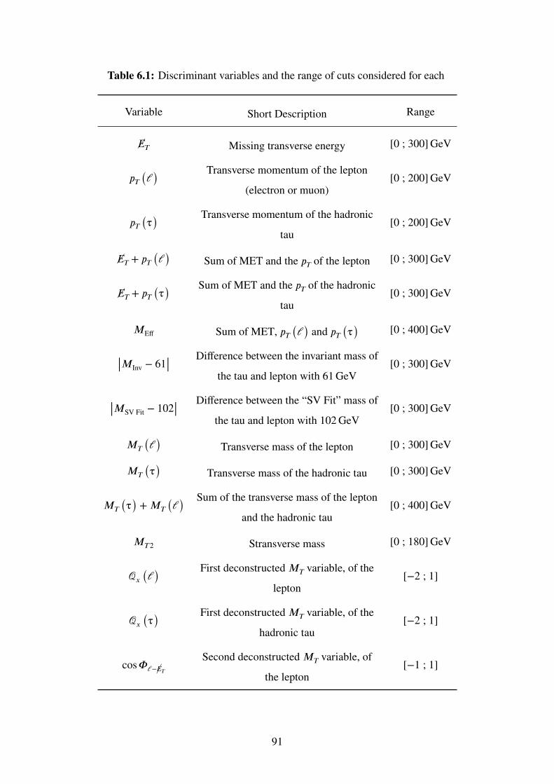
Table 6.1: Discriminant variables and the range of cuts considered for each

Variable Short Description Range

�E𝑇 Missing transverse energy [0 ; 300]GeV

𝑝𝑇 (ℓ)Transverse momentum of the lepton

(electron or muon)[0 ; 200]GeV

𝑝𝑇 (τ)Transverse momentum of the hadronic

tau[0 ; 200]GeV

�E𝑇 + 𝑝𝑇 (ℓ) Sum of MET and the 𝑝𝑇 of the lepton [0 ; 300]GeV

�E𝑇 + 𝑝𝑇 (τ)Sum of MET and the 𝑝𝑇 of the hadronic

tau[0 ; 300]GeV

𝑀Eff Sum of MET, 𝑝𝑇 (ℓ) and 𝑝𝑇 (τ) [0 ; 400]GeV

|𝑀Inv − 61|Difference between the invariant mass of

the tau and lepton with 61GeV[0 ; 300]GeV

|𝑀SV Fit − 102|Difference between the “SV Fit” mass of

the tau and lepton with 102GeV[0 ; 300]GeV

𝑀𝑇 (ℓ) Transverse mass of the lepton [0 ; 300]GeV

𝑀𝑇 (τ) Transverse mass of the hadronic tau [0 ; 300]GeV

𝑀𝑇 (τ) + 𝑀𝑇 (ℓ)Sum of the transverse mass of the lepton

and the hadronic tau[0 ; 400]GeV

𝑀𝑇 2 Stransverse mass [0 ; 180]GeV

𝒬𝑥 (ℓ)First deconstructed 𝑀𝑇 variable, of the

lepton[−2 ; 1]

𝒬𝑥 (τ)First deconstructed 𝑀𝑇 variable, of the

hadronic tau[−2 ; 1]

cos𝛷ℓ−�E𝑇

Second deconstructed 𝑀𝑇 variable, of

the lepton[−1 ; 1]

91

Table 6.1: Discriminant variables and the range of cuts considered for each

(continued)

Variable Short Description Range

cos𝛷τ−�E𝑇

Second deconstructed 𝑀𝑇 variable, of the

hadronic tau[−1 ; 1]

𝒬𝑥 (ℓ) + cos𝛷ℓ−�E𝑇

Sum of the deconstructed 𝑀𝑇 variables, of

the lepton[−3 ; 2]

𝒬𝑥 (τ) + cos𝛷τ−�E𝑇

Sum of the deconstructed 𝑀𝑇 variables, of

the hadronic tau[−3 ; 2]

|𝛥𝛷ℓ−τ|Difference of the azimuthal angle between

the lepton and the tau[0 ; 𝜋]

𝛥𝛷ℓτ−�E𝑇

Difference of the azimuthal angle between the

MET and the system of the lepton and the tau[0 ; 𝜋]

𝛥𝑅ℓ−τ 𝛥𝑅 between the hadronic tau and the lepton [0 ; 5]

|cos 𝜃τ|Cosine of the angle between the tau and the

beam-line[0 ; 1]

|cos 𝜃ℓ|Cosine of the angle between the lepton and

the beam-line[0 ; 1]

the higher the transverse momentum is expected to be, see Fig. 6.2. The transverse momentum

variables are thus good candidates for discriminant variables, however it is expected that they

will have a larger importance for the higher 𝛥𝑀 regions. Note that, for signal, the 𝑝𝑇 (ℓ) dis-

tribution is slightly softer than the 𝑝𝑇 (τ) distribution, which is likely associated with the extra

neutrino in the leptonic decay of the tau when compared to the hadronic decay of the tau.

For the same reasons explained for the MET and transverse momentum variables, the sums

�E𝑇 + 𝑝𝑇 (ℓ), �E𝑇 + 𝑝𝑇 (τ) and 𝑀Eff ≡ �E𝑇 + 𝑝𝑇 (ℓ) + 𝑝𝑇 (τ) are expected to increase as 𝛥𝑀

increases, see Fig. 6.3. As a result, they are good candidates for discriminant variables.

To handle the large DY SM background, a discriminant variable targeted to this process is

92

MET0 100 200 300

% E

vent

s

4−10

3−10

2−10

1−10

Single top

tt

VV/VVV

+ Jetsγ

QCD

ll→Z

W + Jets

M=20∆

M=50∆

M=100∆

M=200∆

=8.0 TeVs

Figure 6.1: The �E𝑇 discriminant variable after preselection level for the MC sum and for 4 dif-

ferent 𝛥𝑀 signal points. The considered background MC processes are stacked and the sum is

normalised to unity. Each signal sample is independently normalised to unity. All MC samples

are corrected by the relevant scale factors.

)τ(T

p0 50 100 150 200

% E

vent

s

4−10

3−10

2−10

1−10

Single top

tt

VV/VVV

+ Jetsγ

QCD

ll→Z

W + Jets

M=20∆

M=50∆

M=100∆

M=200∆

=8.0 TeVs

(a) 𝑝𝑇 (τ)

(l)T

p0 50 100 150 200

% E

vent

s

4−10

3−10

2−10

1−10

Single top

tt

VV/VVV

+ Jetsγ

QCD

ll→Z

W + Jets

M=20∆

M=50∆

M=100∆

M=200∆

=8.0 TeVs

(b) 𝑝𝑇 (ℓ)

Figure 6.2: The 𝑝𝑇 (τ) and 𝑝𝑇 (ℓ) discriminant variables after preselection level for the MC

sum and for 4 different 𝛥𝑀 signal points. The considered backgroundMC processes are stacked

and the sum is normalised to unity. Each signal sample is independently normalised to unity.

All MC samples are corrected by the relevant scale factors.

93

)τ(T

MET+p0 100 200 300

% E

vent

s

4−10

3−10

2−10

1−10

Single top

tt

VV/VVV

+ Jetsγ

QCD

ll→Z

W + Jets

M=20∆

M=50∆

M=100∆

M=200∆

=8.0 TeVs

(a) �E𝑇 + 𝑝𝑇 (τ)

(l)T

MET+p0 100 200 300

% E

vent

s4−10

3−10

2−10

1−10Single top

tt

VV/VVV

+ Jetsγ

QCD

ll→Z

W + Jets

M=20∆

M=50∆

M=100∆

M=200∆

=8.0 TeVs

(b) �E𝑇 + 𝑝𝑇 (ℓ)

EffM0 100 200 300 400

% E

vent

s

4−10

3−10

2−10

1−10Single top

tt

VV/VVV

+ Jetsγ

QCD

ll→Z

W + Jets

M=20∆

M=50∆

M=100∆

M=200∆

=8.0 TeVs

(c) 𝑀Eff

Figure 6.3: The �E𝑇 + 𝑝𝑇 (τ) , �E𝑇 + 𝑝𝑇 (ℓ) and 𝑀Eff discriminant variables after preselection

level for the MC sum and for 4 different 𝛥𝑀 signal points. The considered background MC

processes are stacked and the sum is normalised to unity. Each signal sample is independently

normalised to unity. All MC samples are corrected by the relevant scale factors.

94

InvM0 100 200 300

% E

vent

s

4−10

3−10

2−10

1−10Single top

tt

VV/VVV

+ Jetsγ

QCD

ll→Z

W + Jets

M=20∆

M=50∆

M=100∆

M=200∆

=8.0 TeVs

Figure 6.4: The 𝑀Inv discriminant variable after preselection level for the MC sum and for 4

different 𝛥𝑀 signal points. The considered backgroundMC processes are stacked and the sum is



introduced. In this process, since both taus originate from the Z boson, the invariant mass of

the decay products is expected to reconstruct the mass of the Z boson. However, not all of the

decay products are directly measured since the decay products include neutrinos, so only the

visible decay products are considered. The base of the discriminant variable is the invariant

mass of the reconstructed hadronic τ and the reconstructed lepton (electron or muon). Using the

MC simulation of the DY process, it is verified that the peak of the invariant mass distribution

is shifted down to 61GeV, Fig. 6.5a. The same is not true for the signal process since they

do not result from the same resonance, consequently a cut on the invariant mass distribution

in a window around 61GeV, the variable |𝑀Inv − 61|, can be effective in reducing the DY SM

background for certain 𝛥𝑀 values and is used as a discriminant variable, see Fig. 6.4.

As an alternative to the invariant mass, the mass computed with the “SV Fit” algorithm can

also be used. The algorithm is fully described in [89], it performs a maximum likelihood fit for

each event to estimate the mass of a mother particle which decays to two taus, using the MET

and the transverse momentum of the lepton and hadronic tau. The peak of the distribution for

the DY SM background is observed to lie at 102GeV, Fig. 6.5b, so the discriminant variable is

defined in such a way to define a window around this value, i.e. |𝑀SV Fit − 102|, see Fig. 6.6.

The transverse mass variables, 𝑀𝑇 (𝑥), are traditional variables used to determine the mass

95

InvMass FitConstant 75.1± 8837

Mean 0.09± 61.25

Sigma 0.06± 12.46

τl-M0 100 200 300 400 500

Eve

nts

0

1000

2000

3000

4000

5000

6000

7000

8000

9000 / ndf 2χ 268.5 / 5

Constant 75.1± 8837

Mean 0.09± 61.25

Sigma 0.06± 12.46

(a) Invariant Mass

SVFitMass Fit / ndf 2χ 1048 / 11


Mean 0.1± 102.4

Sigma 0.11± 18.94

SVFitM0 100 200 300 400 500

Eve

nts

0

1000

2000

3000

4000

5000

6000 / ndf 2χ 1048 / 11


Mean 0.1± 102.4

Sigma 0.11± 18.94

(b) “SV Fit” Mass

Figure 6.5: Mass distributions of the DY MC simulation. The peaks are fitted with a Gaussian

and the fit parameters are listed in a box on the top right.

of a mother particle that decays to an invisible particle and a visible one. They are computed

using the MET and an extra object, Eq. 6.2, the 𝑥 value is used to reference which object, 𝛷𝑥−�E𝑇

is the azimuthal angle between the MET and the object and 𝐸𝑇 (𝑥) is the transverse energy of

that same object. For signal events, given the presence of further invisible particles, the 𝑀𝑇 (𝑥)

distributions are expected to be modified with respect to the SM expectation, see Fig. 6.7. The

same applies to the 𝑀𝑇 (ℓ) + 𝑀𝑇 (τ) discriminant variable.

𝑀2𝑇 (𝑥) = 𝑀2

𝑇 (𝑥,�E𝑇) = 2𝐸𝑇 (𝑥)�E𝑇 (1 − cos𝛷𝑥−�E𝑇) (6.2)

The stransverse mass variable, 𝑀𝑇 2, is a variable specially introduced for SUSY searches

[90, 91], Eq. 6.3. It is introduced in an analogous manner to the 𝑀𝑇 variable, considering that

a pair of particles are produced and each decay to an invisible particle and a visible particle. It

further assumes the two invisible particles have the same mass. Similarly to the 𝑀𝑇 variable,

the endpoint of the 𝑀𝑇 2 variable sets a constraint on the mass of the original particle that is

pair produced. However, the 𝑀𝑇 2 variable takes as input the mass of the invisible particle,

therefore the constraint on themass of themother particle is a function of𝑀LSP. For this analysis,

in the computation of 𝑀𝑇 2, the 𝑀LSP was considered to be zero. 𝑀𝑇 2 is expected to have a

higher endpoint with signal events than with background events, being a good discriminator,

see Fig. 6.8.

𝑀2𝑇 2 = min

�𝑝1+�𝑝2=�𝑝𝑇[max{𝑀2

𝑇 (𝑝𝑇 (ℓ−) ,��𝑝1) , 𝑀2

𝑇 (𝑝𝑇 (ℓ+) ,��𝑝2)}] (6.3)

96

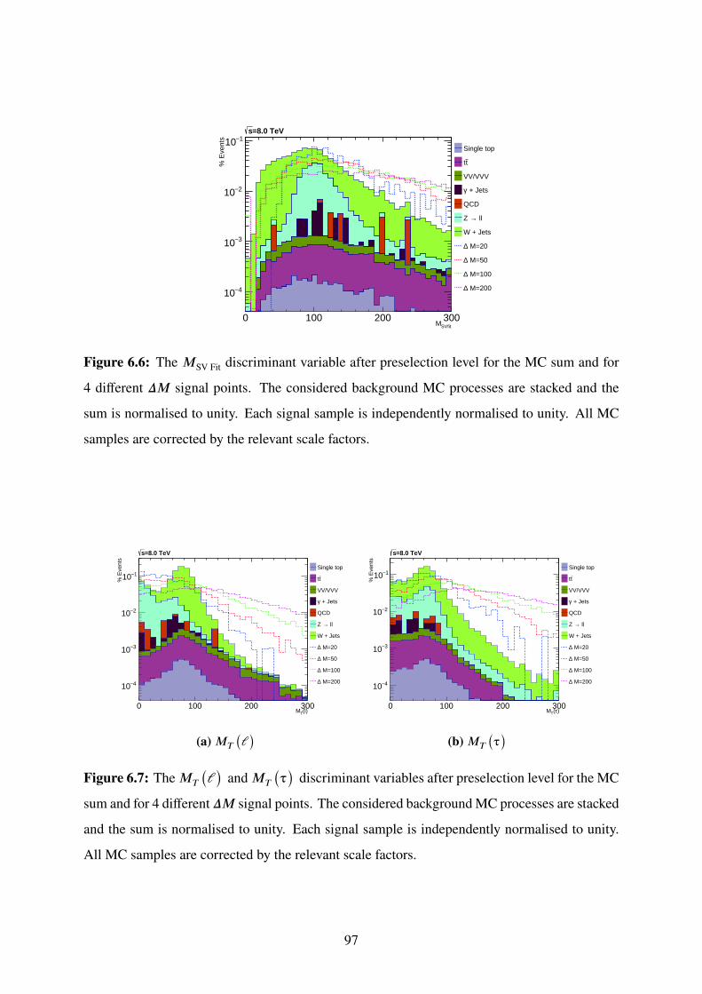
SVfitM0 100 200 300

% E

vent

s

4−10

3−10

2−10

1−10Single top

tt

VV/VVV

+ Jetsγ

QCD

ll→Z

W + Jets

M=20∆

M=50∆

M=100∆

M=200∆

=8.0 TeVs

Figure 6.6: The 𝑀SV Fit discriminant variable after preselection level for the MC sum and for

4 different 𝛥𝑀 signal points. The considered background MC processes are stacked and the

sum is normalised to unity. Each signal sample is independently normalised to unity. All MC

samples are corrected by the relevant scale factors.

(l)TM0 100 200 300

% E

vent

s

4−10

3−10

2−10

1−10Single top

tt

VV/VVV

+ Jetsγ

QCD

ll→Z

W + Jets

M=20∆

M=50∆

M=100∆

M=200∆

=8.0 TeVs

(a) 𝑀𝑇 (ℓ)

)τ(TM0 100 200 300

% E

vent

s

4−10

3−10

2−10

1−10Single top

tt

VV/VVV

+ Jetsγ

QCD

ll→Z

W + Jets

M=20∆

M=50∆

M=100∆

M=200∆

=8.0 TeVs

(b) 𝑀𝑇 (τ)

Figure 6.7: The 𝑀𝑇 (ℓ) and 𝑀𝑇 (τ) discriminant variables after preselection level for the MC




97

T2M0 50 100 150

% E

vent

s

4−10

3−10

2−10

1−10

Single top

tt

VV/VVV

+ Jetsγ

QCD

ll→Z

W + Jets

M=20∆

M=50∆

M=100∆

M=200∆

=8.0 TeVs

Figure 6.8: The 𝑀𝑇 2 discriminant variable after preselection level for the MC sum and for 4

different 𝛥𝑀 signal points. The considered backgroundMC processes are stacked and the sum is



The deconstructed 𝑀𝑇 variables are a set of variables introduced specifically targeted to the

t analysis, yet valuable for any analysis with undetected particles in the final state. They are fully

detailed in [92]. In summary, the variables are obtained from the formula for the 𝑀𝑇 variable,

Eq. 6.4, where 𝛷𝑥−�E𝑇is the azimuthal angle between the MET and the object under considera-

tion and 𝐸𝑇 (𝑥) is the transverse energy of that same object. The formula is rearranged in such

a way that on one side there are only kinematical variables and on the other only topological

ones, Eq. 6.5. Each side of the rearranged equation is now considered one of the deconstructed

𝑀𝑇 variables, Eq. 6.6 and Eq. 6.7, in effect decorrelating the kinematical and topological com-

ponents. From the formula it can be seen that the variable 𝒬 depends upon the 𝑀𝑇 parameter,

which in this approach is not known and must be assumed. The exact value to be used must be

studied on a case by case basis, for this analysis, two possibilities are considered, 𝒬80 (𝑥) and

𝒬100 (𝑥), assuming 𝑀𝑇 = 80GeV and 𝑀𝑇 = 100GeV respectively. These values are recom-

mended by the author of [92], the first value since it is the mass of the W, the second for being

larger than 𝑀 (W) and for serving as a further check. The distribution of these variables can be

98

seen in Fig 6.9 for background and for 4 different 𝛥𝑀 signal points.

𝑀2𝑇 (𝑥) = 2𝐸𝑇 (𝑥)�E𝑇 (1 − cos𝛷𝑥−�E𝑇) (6.4)

1 −𝑀2

𝑇

2𝐸𝑇 (𝑥)�E𝑇= cos𝛷𝑥−�E𝑇

(6.5)

𝒬𝑀𝑇(𝑥) ≡ 1 −

𝑀2𝑇

2𝐸𝑇 (𝑥)�E𝑇(6.6)

cos𝛷𝑥−�E𝑇(6.7)

Considering the correlation plots of the deconstructed 𝑀𝑇 variables for MC for the signal

process and the main SM background processes, Fig. 6.10, it is observed that the two vari-

ables correlate differently for signal and background. Signal tends to cluster at the extremes of

cos𝛷𝑥−�E𝑇and at high values of 𝒬𝑀𝑇

(𝑥), while the two main background processes cluster at one

of the extremes of cos𝛷𝑥−�E𝑇and at lower values of 𝒬𝑀𝑇

(𝑥). Consequently, a cut on a variable

like 𝒬𝑀𝑇(𝑥)+cos𝛷𝑥−�E𝑇

, which attempts to extract more information from the above correlation,

is an interesting prospect for rejecting the background processes, see Fig. 6.11.

In the signal process, the τ particles are pair produced and as a result are mostly back to back,

i.e. 𝛥𝛷τ− τ ≈ 𝜋. For low 𝛥𝑀 values, the decay products from the τ decay do not change direction

significantly from the τ direction and as a result the decay products continue in a mostly back

to back direction, i.e. 𝛥𝛷ℓ−τ ≈ 𝜋. For higher 𝛥𝑀 values, the decay products are more deflected

from the original τ direction, resulting in a smearing of the values for 𝛥𝛷ℓ−τ. For the SM

background processes, the 𝛥𝛷ℓ−τ distribution is fixed according to the process. For example

with W + 1Jet events, where the W decays to a lepton and the jet fakes a tau, the lepton and the

fake tau will be mostly back to back, i.e. 𝛥𝛷ℓ−τ ≈ 𝜋, yet with W + 𝑁Jet events, with 𝑁 > 1, the

lepton and the fake tau are no longer back to back, resulting in lower values for 𝛥𝛷ℓ−τ. These dif-

ferent behaviours for different𝛥𝑀 values and different processes can be exploited to discriminate

among the processes, in particular in conjunction with further discriminant variables. A similar

reasoning can be made for the 𝛥𝛷ℓτ−�E𝑇and 𝛥𝑅ℓ−τ discriminant variables. Fig 6.12 illustrates

these discriminant variables.

The variables cos 𝜃𝑥 have a one-to-one correspondence with 𝜂 (𝑥) ≡ − ln [tan(𝜃𝑥

2 )]. These

variables are not expected to be significantly different between signal and background, how-

ever in combination with other discriminating variables, they can give a better discrimination

99

l-METΦcos1− 0.5− 0 0.5 1

% E

vent

s

4−10

3−10

2−10

1−10Single top

tt

VV/VVV

+ Jetsγ

QCD

ll→Z

W + Jets

M=20∆

M=50∆

M=100∆

M=200∆

=8.0 TeVs

(a) cos𝛷ℓ−�E𝑇

-METτΦcos1− 0.5− 0 0.5 1

% E

vent

s

4−10

3−10

2−10

1−10

Single top

tt

VV/VVV

+ Jetsγ

QCD

ll→Z

W + Jets

M=20∆

M=50∆

M=100∆

M=200∆

=8.0 TeVs

(b) cos𝛷τ−�E𝑇

(l)80

Q2− 1− 0 1

% E

vent

s

4−10

3−10

2−10

1−10Single top

tt

VV/VVV

+ Jetsγ

QCD

ll→Z

W + Jets

M=20∆

M=50∆

M=100∆

M=200∆

=8.0 TeVs

(c) 𝒬80 (ℓ)

)τ(80

Q2− 1− 0 1

% E

vent

s

4−10

3−10

2−10

1−10Single top

tt

VV/VVV

+ Jetsγ

QCD

ll→Z

W + Jets

M=20∆

M=50∆

M=100∆

M=200∆

=8.0 TeVs

(d) 𝒬80 (τ)

(l)100

Q2− 1− 0 1

% E

vent

s

4−10

3−10

2−10

1−10 Single top

tt

VV/VVV

+ Jetsγ

QCD

ll→Z

W + Jets

M=20∆

M=50∆

M=100∆

M=200∆

=8.0 TeVs

(e) 𝒬100 (ℓ)

)τ(100

Q2− 1− 0 1

% E

vent

s

4−10

3−10

2−10

1−10Single top

tt

VV/VVV

+ Jetsγ

QCD

ll→Z

W + Jets

M=20∆

M=50∆

M=100∆

M=200∆

=8.0 TeVs

(f) 𝒬100 (τ)

Figure 6.9: The deconstructed 𝑀𝑇 discriminant variables after preselection level for the MC




100

4−10

3−10

2−10

Φcos1− 0.5− 0 0.5 1

80Q

2−

1.5−

1−

0.5−

0

0.5

1

(a) W + Jets

4−10

3−10

2−10

Φcos1− 0.5− 0 0.5 1

80Q

2−

1.5−

1−

0.5−

0

0.5

1

(b) Z → ℓℓ

Φcos1− 0.5− 0 0.5 1

80Q

2−

1.5−

1−

0.5−

0

0.5

1

6−10

5−10

4−10

(c) Signal – 𝛥𝑀 = 50GeV

Φcos1− 0.5− 0 0.5 1

80Q

2−

1.5−

1−

0.5−

0

0.5

1

7−10

6−10

5−10

(d) Signal – 𝛥𝑀 = 200GeV

Figure 6.10: Correlation of the deconstructed 𝑀𝑇 variables at preselection level for the main

background processes and for signal, for two 𝛥𝑀 values. The considered deconstructed 𝑀𝑇

variables are: 𝒬80 (ℓ) and cos𝛷ℓ−�E𝑇.

since the multi-dimensional correlation among the many variables is hard to visualise from first

principles. Fig. 6.13 shows the distribution of these variables for signal and background.

Some of the discriminating variables in Table 6.1 are compound variables, obtained through

the combination of several simpler variables. Figure 6.14 shows the distributions of some of the

discriminant variables, those used in subsequent sections, in MC events compared to data at the

preselection level.

101

l-METΦ(l)+cos80

Q3− 2− 1− 0 1 2

% E

vent

s

4−10

3−10

2−10

1−10Single top

tt

VV/VVV

+ Jetsγ

QCD

ll→Z

W + Jets

M=20∆

M=50∆

M=100∆

M=200∆

=8.0 TeVs

(a) 𝒬80 (ℓ) + cos𝛷ℓ−�E𝑇

-METτΦ)+cosτ(

80Q

3− 2− 1− 0 1 2

% E

vent

s4−10

3−10

2−10

1−10

Single top

tt

VV/VVV

+ Jetsγ

QCD

ll→Z

W + Jets

M=20∆

M=50∆

M=100∆

M=200∆

=8.0 TeVs

(b) 𝒬80 (τ) + cos𝛷τ−�E𝑇

l-METΦ(l)+cos100

Q3− 2− 1− 0 1 2

% E

vent

s

4−10

3−10

2−10

1−10 Single top

tt

VV/VVV

+ Jetsγ

QCD

ll→Z

W + Jets

M=20∆

M=50∆

M=100∆

M=200∆

=8.0 TeVs

(c) 𝒬100 (ℓ) + cos𝛷ℓ−�E𝑇

-METτΦ)+cosτ(

100Q

3− 2− 1− 0 1 2

% E

vent

s

4−10

3−10

2−10

1−10

Single top

tt

VV/VVV

+ Jetsγ

QCD

ll→Z

W + Jets

M=20∆

M=50∆

M=100∆

M=200∆

=8.0 TeVs

(d) 𝒬100 (τ) + cos𝛷τ−�E𝑇

Figure 6.11: The correlated deconstructed 𝑀𝑇 discriminant variables after preselection level

for the MC sum and for 4 different 𝛥𝑀 signal points. The considered background MC processes

are stacked and the sum is normalised to unity. Each signal sample is independently normalised

to unity. All MC samples are corrected by the relevant scale factors.

102

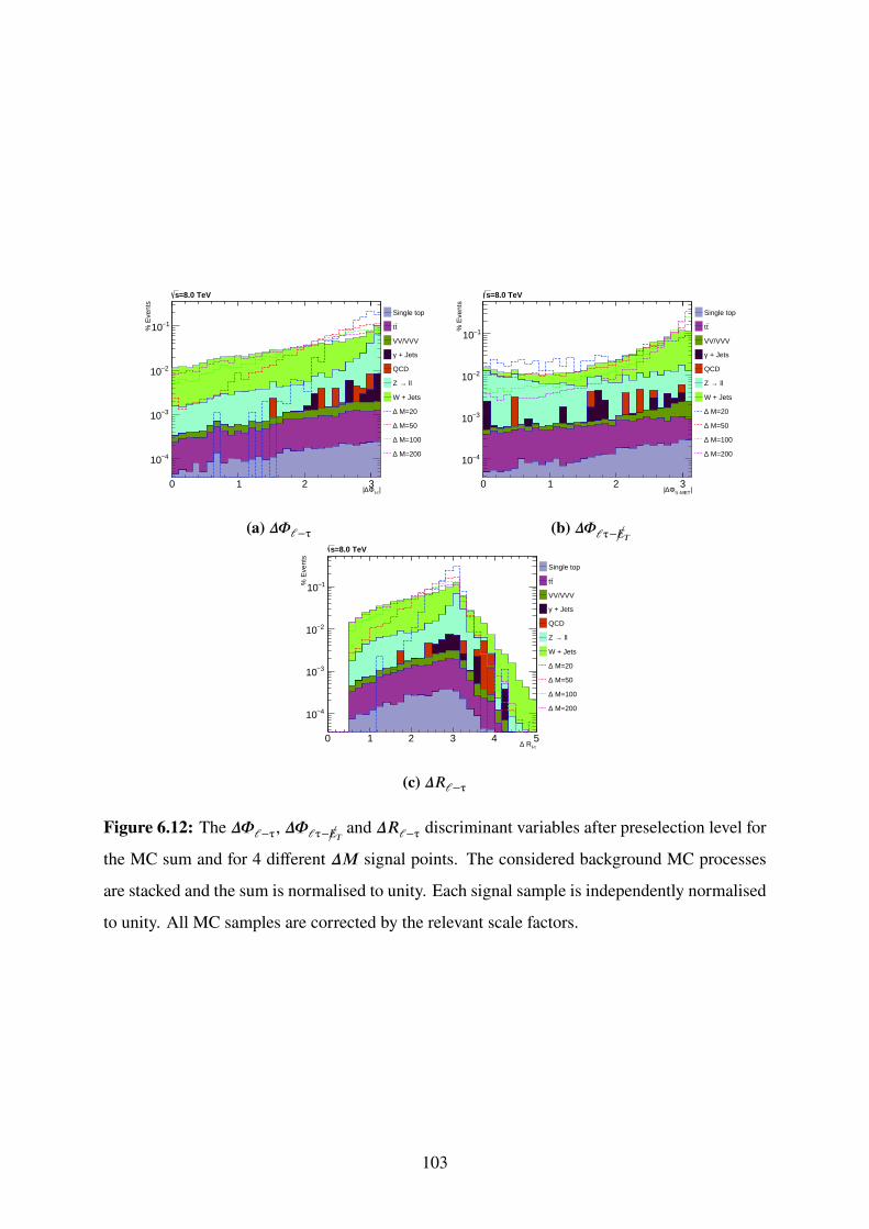
|τl-Φ∆|0 1 2 3

% E

vent

s

4−10

3−10

2−10

1−10

Single top

tt

VV/VVV

+ Jetsγ

QCD

ll→Z

W + Jets

M=20∆

M=50∆

M=100∆

M=200∆

=8.0 TeVs

(a) 𝛥𝛷ℓ−τ

|-METτlΦ∆|0 1 2 3

% E

vent

s4−10

3−10

2−10

1−10

Single top

tt

VV/VVV

+ Jetsγ

QCD

ll→Z

W + Jets

M=20∆

M=50∆

M=100∆

M=200∆

=8.0 TeVs

(b) 𝛥𝛷ℓτ−�E𝑇

τl- R∆0 1 2 3 4 5

% E

vent

s

4−10

3−10

2−10

1−10

Single top

tt

VV/VVV

+ Jetsγ

QCD

ll→Z

W + Jets

M=20∆

M=50∆

M=100∆

M=200∆

=8.0 TeVs

(c) 𝛥𝑅ℓ−τ

Figure 6.12: The 𝛥𝛷ℓ−τ, 𝛥𝛷ℓτ−�E𝑇and 𝛥𝑅ℓ−τ discriminant variables after preselection level for

the MC sum and for 4 different 𝛥𝑀 signal points. The considered background MC processes

are stacked and the sum is normalised to unity. Each signal sample is independently normalised

to unity. All MC samples are corrected by the relevant scale factors.

103

lθcos 0 0.2 0.4 0.6 0.8 1

% E

vent

s

4−10

3−10

2−10

1−10Single top

tt

VV/VVV

+ Jetsγ

QCD

ll→Z

W + Jets

M=20∆

M=50∆

M=100∆

M=200∆

=8.0 TeVs

(a) cos 𝜃ℓ

τθcos 0 0.2 0.4 0.6 0.8 1

% E

vent

s

4−10

3−10

2−10

1−10 Single top

tt

VV/VVV

+ Jetsγ

QCD

ll→Z

W + Jets

M=20∆

M=50∆

M=100∆

M=200∆

=8.0 TeVs

(b) cos 𝜃τ

Figure 6.13: The cos 𝜃ℓ and cos 𝜃τ discriminant variables after preselection level for the MC




6.1.2 Cut Selection Procedure

The cut selection procedure is performed for all the 𝛥𝑀 samples, but each 𝛥𝑀 sample is treated

separately. The procedure starts by scanning for each variable, var, the values, 𝑋, within the

variable’s defined range. For each value, cuts of the type var > 𝑋 and var < 𝑋 are considered.

For each cut, the signal and background yields are computed, n.b. for signal there is a yield for

each 𝛥𝑀 sample. The yields are subsequently used to compute a Figure of Merit (FOM), n.b.

once again there is a FOM for each 𝛥𝑀 sample. The FOM quantifies the expected significance

of the selection after the statistical analysis. It is used instead of the statistical analysis since it

is quicker and easier to perform and in this way it is used as a surrogate for the full statistical

analysis. Once the scan is finalised, the variable, cut value and cut direction with the highest

FOM is chosen as the optimal cut for that 𝛥𝑀 sample.

The FOM used for this analysis is summarised in Equation 6.8, where 𝑁𝐵 is the expected

background yield and 𝑁𝑆 is the expected signal yield. This FOM is further detailed in [93]. This

particular FOM was chosen for being the most performant one known by the author at the time.

FOM = 2 × (√(𝑁𝑆 + 𝑁𝐵) − √(𝑁𝐵)) (6.8)

The above-described procedure is then iteratively repeated, with the care that for each 𝛥𝑀

104

(l)T

MET+p0 100 200 300

Eve

nts

2−10

1−10

1

10

210

310

410Single top

tt

VV/VVV

+ Jetsγ

QCD

ll→Z

W + Jets

TStauStau_120_20

data

-1 L=19.7 fb∫=8.0 TeV, s

0 100 200 300

MC

ΣD

ata/ 0.5

1

1.5

(a) �E𝑇 + 𝑝𝑇 (ℓ)

)τ(T

MET+p0 100 200 300

Eve

nts

2−10

1−10

1

10

210

310

410Single top

tt

VV/VVV

+ Jetsγ

QCD

ll→Z

W + Jets

TStauStau_120_20

data

-1 L=19.7 fb∫=8.0 TeV, s

0 100 200 300

MC

ΣD

ata/ 0.5

1

1.5

(b) �E𝑇 + 𝑝𝑇 (τ)

EffM0 100 200 300 400

Eve

nts

2−10

1−10

1

10

210

310

410Single top

tt

VV/VVV

+ Jetsγ

QCD

ll→Z

W + Jets

TStauStau_120_20

data

-1 L=19.7 fb∫=8.0 TeV, s

0 100 200 300 400

MC

ΣD

ata/ 0.5

1

1.5

(c) 𝑀Eff

lθcos 0 0.2 0.4 0.6 0.8 1

Eve

nts

2−10

1−10

1

10

210

310

410 Single top

tt

VV/VVV

+ Jetsγ

QCD

ll→Z

W + Jets

TStauStau_120_20

data

-1 L=19.7 fb∫=8.0 TeV, s

0 0.2 0.4 0.6 0.8 1

MC

ΣD

ata/ 0.5

1

1.5

(d) |cos 𝜃ℓ|

τθcos 0 0.2 0.4 0.6 0.8 1

Eve

nts

2−10

1−10

1

10

210

310

410 Single top

tt

VV/VVV

+ Jetsγ

QCD

ll→Z

W + Jets

TStauStau_120_20

data

-1 L=19.7 fb∫=8.0 TeV, s

0 0.2 0.4 0.6 0.8 1

MC

ΣD

ata/ 0.5

1

1.5

(e) |cos 𝜃τ| (f) 𝑀𝑇 (ℓ) + 𝑀𝑇 (τ)

Figure 6.14: Compound variables after Preselection level, the considered MC processes are

stacked and compared to data. Data corresponds to 19.7 fb−1 of certified CMS data and MC is

scaled to the same luminosity value. All MC samples are corrected by the relevant scale factors.

105

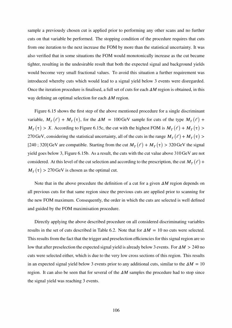
sample a previously chosen cut is applied prior to performing any other scans and no further

cuts on that variable be performed. The stopping condition of the procedure requires that cuts

from one iteration to the next increase the FOM by more than the statistical uncertainty. It was

also verified that in some situations the FOM would monotonically increase as the cut became

tighter, resulting in the undesirable result that both the expected signal and background yields

would become very small fractional values. To avoid this situation a further requirement was

introduced whereby cuts which would lead to a signal yield below 3 events were disregarded.

Once the iteration procedure is finalised, a full set of cuts for each 𝛥𝑀 region is obtained, in this

way defining an optimal selection for each 𝛥𝑀 region.

Figure 6.15 shows the first step of the above mentioned procedure for a single discriminant

variable, 𝑀𝑇 (ℓ) + 𝑀𝑇 (τ), for the 𝛥𝑀 = 100GeV sample for cuts of the type 𝑀𝑇 (ℓ) +

𝑀𝑇 (τ) > 𝑋. According to Figure 6.15c, the cut with the highest FOM is 𝑀𝑇 (ℓ) + 𝑀𝑇 (τ) >

270GeV, considering the statistical uncertainty, all of the cuts in the range 𝑀𝑇 (ℓ) + 𝑀𝑇 (τ) >

[240 ; 320]GeV are compatible. Starting from the cut 𝑀𝑇 (ℓ) + 𝑀𝑇 (τ) > 320GeV the signal

yield goes below 3, Figure 6.15b. As a result, the cuts with the cut value above 310GeV are not

considered. At this level of the cut selection and according to the prescription, the cut 𝑀𝑇 (ℓ) +

𝑀𝑇 (τ) > 270GeV is chosen as the optimal cut.

Note that in the above procedure the definition of a cut for a given 𝛥𝑀 region depends on

all previous cuts for that same region since the previous cuts are applied prior to scanning for

the new FOM maximum. Consequently, the order in which the cuts are selected is well defined

and guided by the FOM maximisation procedure.

Directly applying the above described procedure on all considered discriminating variables

results in the set of cuts described in Table 6.2. Note that for 𝛥𝑀 = 10 no cuts were selected.

This results from the fact that the trigger and preselection efficiencies for this signal region are so

low that after preselection the expected signal yield is already below 3 events. For 𝛥𝑀 > 240 no

cuts were selected either, which is due to the very low cross sections of this region. This results

in an expected signal yield below 3 events prior to any additional cuts, similar to the 𝛥𝑀 = 10

region. It can also be seen that for several of the 𝛥𝑀 samples the procedure had to stop since

the signal yield was reaching 3 events.

106

)τ(T

(l)+MTM0 50 100 150 200 250 300 350 400

Bac

kgro

undY

ield

210

310

410

510

(a) Background Yield

)τ(T

(l)+MTM0 50 100 150 200 250 300 350 400

Sig

nalY

ield

1

10

(b) Signal Yield

(c) Figure of Merit

Figure 6.15: First step of the cut selection prescription for the variable 𝑀𝑇 (ℓ) + 𝑀𝑇 (τ) and

𝛥𝑀 = 100GeV. For a given value on the x-axis, the value read off the y-axis is the yield (or

FOM) after applying a cut with the given value. The signal and background yields are computed

fromMC simulation scaled to the luminosity of 19.7 fb−1. The background yield is given by the

sum of the yields of the individual background processes. The signal yield is computed with the

prescription given at the beginning of Chapter 6. The FOM is computed according to Eq. 6.8.

6.1.3 Cut Simplification

It is clear from Table 6.2 that applying the full cut selection as described, i.e. a different selec-

tion for each 𝛥𝑀 value, is very complex with several different sets of cuts, all using different

discriminant variables. Applying such a large set of cuts is also both time and resource inten-

sive. With the intent of keeping a minimal set of cuts, but sacrificing as little as possible in the

performance of the analysis, a slightly modified cut selection procedure is used, however with-

107

Table 6.2: Direct application of the iterative cut selection procedure. All dimension-full cuts

are in units ofGeV. The signal and background yields are computed fromMC simulation scaled

to the luminosity of 19.7 fb−1. The background yield is given by the sum of the yields of the

individual background processes. The signal yield is computed with the prescription given at the

beginning of Chapter 6. The FOM is computed according to Eq. 6.8. The cuts are successively

applied, starting with Cut 1.

𝛥𝑀 Cut 1 Cut 2 Cut 3 Cut 4 Cut 5 𝑁𝑆 𝑁𝐵 FOM

10 – – – – – – – –

20 𝛥𝜙𝑙−𝜏> 2.33 𝑀𝐸𝑇 + 𝑝𝑇(𝜏)> 100 |𝑀𝐼𝑛𝑣 − 61|< 70 𝑀𝑇 2< 40 – 3.030 ± 0.169 3841 ± 87 0.048 87 ± 0.002 78

30 𝑄80(𝜏)> −0.3 𝛥𝜙𝑙−𝜏> 2.43 |𝑀𝐼𝑛𝑣 − 61|< 50 𝛥𝛼𝑙−𝜏> 1.22 𝑀𝐸𝑇 + 𝑝𝑇(𝜏)> 120 3.124 ± 0.154 605 ± 29 0.126 76 ± 0.006 98

40 𝑄100(𝜏)> −0.7 𝛥𝜙𝑙−𝜏> 2.33 |𝑀𝐼𝑛𝑣 − 61|< 120 𝑐𝑜𝑠𝜃𝜏< 0.9 – 9.182 ± 0.233 2950 ± 80 0.168 90 ± 0.004 86

50 𝑀𝐸𝑇 + 𝑝𝑇(𝜏)> 130 𝛥𝜙𝑙−𝜏> 2.23 𝑐𝑜𝑠𝜃𝜏< 0.9 – – 11.157 ± 0.227 2761 ± 75 0.212 10 ± 0.005 19

60 𝑄100(𝜏)> 0 𝛥𝜙𝑙−𝜏> 1.92 𝑐𝑜𝑠𝜃𝜏< 0.9 – – 9.782 ± 0.197 1965 ± 63 0.220 40 ± 0.005 69

70 𝑀𝑇(𝑙) + 𝑀𝑇(𝜏)> 230 𝑄80(𝜏) + 𝑐𝑜𝑠𝛷(𝜏)> −0.33 𝛥𝛼𝑙−𝜏> 1.11 – – 7.078 ± 0.154 959 ± 41 0.228 08 ± 0.006 94

80 𝑀𝑇(𝑙) + 𝑀𝑇(𝜏)> 240 𝑐𝑜𝑠𝜃𝑙< 0.9 – – – 7.578 ± 0.135 1156 ± 45 0.222 50 ± 0.005 90

90 𝑀𝑇(𝑙) + 𝑀𝑇(𝜏)> 270 𝑐𝑜𝑠𝜃𝑙< 0.9 – – – 5.871 ± 0.106 538 ± 28 0.252 28 ± 0.008 05

100 𝑀𝑇(𝑙) + 𝑀𝑇(𝜏)> 300 𝑀𝑇(𝜏)> 60 𝑐𝑜𝑠𝜃𝑙< 0.9 – – 4.546 ± 0.083 230 ± 19 0.298 03 ± 0.013 37

110 𝑀𝑇(𝑙) + 𝑀𝑇(𝜏)> 300 𝑀𝑇(𝜏)> 70 – – – 4.625 ± 0.075 281 ± 21 0.274 63 ± 0.011 51

120 𝑀𝑇(𝑙) + 𝑀𝑇(𝜏)> 330 𝑀𝑇(𝜏)> 80 – – – 3.684 ± 0.068 144 ± 14 0.304 66 ± 0.016 25

130 𝑀𝑇(𝑙) + 𝑀𝑇(𝜏)> 330 𝑀𝑇(𝜏)> 80 – – – 3.476 ± 0.054 144 ± 14 0.287 64 ± 0.015 07

140 𝑀𝑇(𝑙) + 𝑀𝑇(𝜏)> 330 𝑀𝑇(𝜏)> 80 – – – 3.406 ± 0.047 144 ± 14 0.281 88 ± 0.014 64

150 𝑀𝑇(𝑙) + 𝑀𝑇(𝜏)> 330 𝑀𝑇(𝜏)> 80 𝑄100(𝑙)> 0 – – 3.080 ± 0.044 111 ± 11 0.290 28 ± 0.015 86

160 𝑀𝑇(𝑙) + 𝑀𝑇(𝜏)> 330 𝑀𝑇(𝜏)> 80 – – – 3.076 ± 0.041 144 ± 14 0.254 63 ± 0.013 20

170 𝑀𝑇(𝑙) + 𝑀𝑇(𝜏)> 330 𝑀𝑇(𝜏)> 50 – – – 3.022 ± 0.036 161 ± 14 0.236 33 ± 0.011 12

180 𝑀𝑇(𝑙) + 𝑀𝑇(𝜏)> 310 𝑀𝑇(𝜏)> 60 – – – 3.026 ± 0.035 237 ± 19 0.195 89 ± 0.008 32

190 𝑀𝑇(𝑙) + 𝑀𝑇(𝜏)> 300 – – – – 3.069 ± 0.033 365 ± 22 0.160 29 ± 0.005 26

200 𝑀𝑇(𝑙) + 𝑀𝑇(𝜏)> 280 – – – – 3.023 ± 0.031 547 ± 29 0.129 06 ± 0.003 66

210 𝑀𝑇(𝑙) + 𝑀𝑇(𝜏)> 250 𝑄100(𝑙)> −0.5 – – – 3.006 ± 0.028 940 ± 40 0.097 90 ± 0.002 29

220 𝑀𝑇(𝑙) + 𝑀𝑇(𝜏)> 240 – – – – 3.012 ± 0.028 1429 ± 51 0.079 63 ± 0.001 62

230 𝑀𝑇(𝑙) + 𝑀𝑇(𝜏)> 210 – – – – 3.004 ± 0.027 3389 ± 86 0.051 59 ± 0.000 80

240 𝑄80(𝜏)> −1.6 𝑄80(𝜏) + 𝑐𝑜𝑠𝛷(𝜏)> −2.33 𝑀𝑇(𝑙) + 𝑀𝑇(𝜏)> 50 – – 3.000 ± 0.025 75 824 ± 844 0.010 90 ± 0.000 11

250 – – – – – – – –

260 – – – – – – – –

270 – – – – – – – –

280 – – – – – – – –

290 – – – – – – – –

300 – – – – – – – –

310 – – – – – – – –

320-330 – – – – – – – –

340-350 – – – – – – – –

360-370 – – – – – – – –

380-390 – – – – – – – –

400-410 – – – – – – – –

420-440 – – – – – – – –

>440 – – – – – – – –

out being as automated as the previously described procedure. The modified procedure involves

at each iteration step comparing the evolution of the FOM for each 𝛥𝑀 sample and its neigh-

bouring 𝛥𝑀 samples and choosing a cut in common for as many neighbouring 𝛥𝑀 samples as

possible, always taking care that the FOM is not significantly different from the maximum FOM

108

for those samples. An effort was also made to involve subset of discriminant variables as small

as possible while still maintaining reasonable performance.

In this modified procedure the 𝛥𝑀 = 10GeV sample was purposefully given the same

cuts as the 𝛥𝑀 = 20GeV sample. For the 𝛥𝑀 = 240GeV sample, for the first iteration the

constraint of a signal yield of 3 events was changed to 4 events. All sampleswith𝛥𝑀 > 240GeV

were given the same cuts as the 𝛥𝑀 = 240GeV sample.

In this way 5 distinct sets of cuts were defined, summarised in Table 6.3. The table also

defines the labels used to identify each set of cuts. The signal yields and FOM for each 𝛥𝑀

sample is summarised in Table 6.4.

Table 6.3: Simplified set of cuts per 𝛥𝑀 region. The units for the dimension-full cuts are in

GeV. The background yields are computed from MC simulation scaled to the luminosity of

19.7 fb−1. The background yield is given by the sum of the yields of the individual background

processes.

Label 𝛥𝑀 Range [GeV] Iteration 1 Iteration 2 Iteration 3 Iteration 4 Iteration 5 𝑁𝐵

𝐶1 [10 ; 60] �E𝑇 + 𝑝𝑇 (τ) > 130 𝛥𝛷ℓ−τ > 2 cos 𝜃τ < 0.9 |𝑀Inv − 61| < 120 𝑀𝑇 2 < 35 1243 ± 44

𝐶2 [70 ; 110] 𝑀𝑇 (ℓ) + 𝑀𝑇 (τ) > 260 cos 𝜃ℓ < 0.9 𝑀𝑇 (τ) > 60 �E𝑇 + 𝑝𝑇 (ℓ) > 140 – 458 ± 28

𝐶3 [120 ; 170] 𝑀𝑇 (ℓ) + 𝑀𝑇 (τ) > 285 𝑀𝑇 (τ) > 60 𝑀𝑇 (ℓ) > 90 �E𝑇 + 𝑝𝑇 (τ) > 160 – 126 ± 12

𝐶4 [180 ; 230] 𝑀𝑇 (ℓ) + 𝑀𝑇 (τ) > 210 𝑀Eff > 240 �E𝑇 > 80 𝑀𝑇 (τ) > 80 – 580 ± 32

𝐶5 ≥ 240 𝑀Eff > 110 �E𝑇 + 𝑝𝑇 (τ) > 70 𝑀𝑇 (ℓ) + 𝑀𝑇 (τ) > 50 – – 72 604 ± 841

109

Table 6.4: Signal yield and FOM for each𝛥𝑀 sample after the

modified cut selection procedure. The signal yield is computed

from MC simulation scaled to the luminosity of 19.7 fb−1. It

is computed with the prescription given at the beginning of

Chapter 6. The FOM is computed according to Eq. 6.8.

𝛥𝑀 Cuts 𝑁𝑆 FOM

10 𝐶1 0.22 ± 0.06 0.0063 ± 0.0018

20 𝐶1 1.62 ± 0.12 0.0460 ± 0.0036

30 𝐶1 4.26 ± 0.18 0.1208 ± 0.0055

40 𝐶1 6.15 ± 0.19 0.1743 ± 0.0062

50 𝐶1 7.07 ± 0.18 0.2003 ± 0.0062

60 𝐶1 5.48 ± 0.15 0.1832 ± 0.0062

70 𝐶2 4.50 ± 0.13 0.2297 ± 0.0100

80 𝐶2 4.82 ± 0.10 0.2461 ± 0.0096

90 𝐶2 5.70 ± 0.10 0.2655 ± 0.0094

100 𝐶2 6.26 ± 0.10 0.2914 ± 0.0099

110 𝐶2 5.90 ± 0.08 0.2747 ± 0.0092

120 𝐶3 3.51 ± 0.07 0.3103 ± 0.0159

130 𝐶3 3.22 ± 0.05 0.2841 ± 0.0142

140 𝐶3 3.13 ± 0.04 0.2767 ± 0.0137

150 𝐶3 3.08 ± 0.04 0.2724 ± 0.0135

160 𝐶3 2.81 ± 0.04 0.2488 ± 0.0123

170 𝐶3 2.71 ± 0.03 0.2395 ± 0.0118

180 𝐶4 3.00 ± 0.03 0.1612 ± 0.0066

190 𝐶4 3.00 ± 0.03 0.1371 ± 0.0046

200 𝐶4 2.77 ± 0.03 0.1150 ± 0.0033

210 𝐶4 2.53 ± 0.03 0.1047 ± 0.0030

220 𝐶4 2.39 ± 0.02 0.0993 ± 0.0029

230 𝐶4 2.20 ± 0.02 0.0914 ± 0.0026

240 𝐶5 3.00 ± 0.02 0.0111 ± 0.0001

110

6.1.4 Signal Region Definition

Since the FOM is used as a surrogate for the full statistical analysis, it is important to verify if

the selected set of cuts is indeed the most performant set of cuts for the desired signal space.

To this effect, the expected upper limit for each (𝑀τ, 𝑀LSP) mass point is computed using the

asymptotic CLs method1 [94, 95] for all sets of cuts. Figure 6.16a shows for each (𝑀τ, 𝑀LSP)mass point which set of cuts has the best (i.e lowest) expected upper limit, the colour refers to

the numbering of the label of the set of cuts.

Figure 6.16a shows that the sets of cuts 𝐶4 and 𝐶5 are the best in a limited region. Further-

more, the improvement of 𝐶4 and 𝐶5 with respect to the second best cut is small. Consequently,

𝐶4 and 𝐶5 are discarded and Figure 6.16b shows where each set of cuts, from the reduced set

𝐶1, 𝐶2 and 𝐶3, has the best performance.

The three sets of cuts, 𝐶1, 𝐶2 and𝐶3, have very clearly defined regions where each performs

best. Using Figure 6.16b as a guide, three non-exclusive SRs are defined, each to be used for

different 𝛥𝑀 regions:

• SR1 – 𝐶1; 𝛥𝑀 ∈ [10 ; 70]GeV

• SR2 – 𝐶2; 𝛥𝑀 ∈ [80 ; 160]GeV

• SR3 – 𝐶3; 𝛥𝑀 ≥ 170GeV

6.2 Event Yields per Signal Region

For each SR, the observed data yields and the expected background yields, using only MC, as

well as some reference expected signal yields are summarised in Table 6.5. The defined sets of

cuts are clearly effective in reducing the DY background process, bringing it to the same order

of magnitude, or lower, as the tt process. Despite being significantly reduced, the W + Jets

background process continues with a significant yield, constituting the dominant background

process. It makes up at least 50% of the background events. Data and the expected SM back-

1To compute the expected upper limit, the combine tool is used and only statistical uncertainties and the lumi-

nosity systematic uncertainty are considered. The tool is further described in Chapter 9 , where it is used for the

final result

111

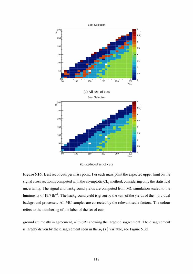
StauM50 100 150 200 250 300

Neu

tM

0

50

100

150

200

250

300

Sel

ectio

n

1

1.5

2

2.5

3

3.5

4

4.5

5

Best Selection

(a) All sets of cuts

StauM50 100 150 200 250 300

Neu

tM

0

50

100

150

200

250

300

Sel

ectio

n

1

1.5

2

2.5

3

3.5

4

4.5

5

Best Selection

(b) Reduced set of cuts

Figure 6.16: Best set of cuts per mass point. For each mass point the expected upper limit on the

signal cross section is computed with the asymptoticCLs method, considering only the statistical

uncertainty. The signal and background yields are computed from MC simulation scaled to the

luminosity of 19.7 fb−1. The background yield is given by the sum of the yields of the individual

background processes. All MC samples are corrected by the relevant scale factors. The colour

refers to the numbering of the label of the set of cuts

ground are mostly in agreement, with SR1 showing the largest disagreement. The disagreement

is largely driven by the disagreement seen in the 𝑝𝑇 (τ) variable, see Figure 5.3d.

112

Table 6.5: Yields per SR. Data corresponds to 19.7 fb−1 of certified CMS

data and MC is scaled to the same luminosity value; the signal MC are

normalised to 𝜎 = 1 pb. For SR1, the signal point𝑀τ = 50GeV; 𝑀LSP =

10GeV is shown, for SR2, the signal point 𝑀τ = 100GeV; 𝑀LSP =

10GeV is shown and for SR3, the signal point 𝑀τ = 180GeV; 𝑀LSP =

10GeV is shown. All MC samples are corrected by the relevant scale

factors.

Process SR1 SR2 SR3

Single top 33.35 ± 3.81 15.96 ± 2.59 4.61 ± 1.33

t t 224.42 ± 12.42 59.22 ± 6.35 24.09 ± 4.03

VV/VVV 66.58 ± 1.90 40.25 ± 1.44 20.94 ± 1.03

γ + Jets 0 0.42 ± 0.34 0.24 ± 0.21

QCD 0 0.22 ± 0.20 0.20 ± 0.20

Z → ℓℓ 230.32 ± 16.30 39.70 ± 6.71 4.61 ± 1.23

W + Jets 688.46 ± 38.49 302.82 ± 26.25 71.85 ± 11.27

Total Expected 1243.13 ± 43.81 458.59 ± 27.99 126.54 ± 12.15

Signal 5.32 ± 3.07 47.11 ± 10.48 122.50 ± 15.00

Data 1107 ± 33 421 ± 20 131 ± 11

113

Chapter 7

Data Driven Background Estimation

The slight mismodelling of the 𝑝𝑇 (τ), see Figure 5.3d, prompts for a more robust method to

estimate the SM background rather than relying only on MC. The W + Jets process accounts

for roughly two thirds, see Table 5.5 (at preselection) and Table 6.5 (at each of the SRs), of the

SM background. Most of the W + Jets events passing preselection are expected to contain a so-

called fake tau. Thus, it is expected that a large fraction of the SM background originates from

fake taus. A fake tau is defined as some object, not a tau, which given the detector efficiency

and event PU is reconstructed as an hadronic tau. Since the tau reconstruction uses the HPS

algorithm, the majority of the fake taus are expected to result from jets. In contrast to fake taus,

a prompt tau is defined as a tau object which is reconstructed as an actual tau.

To better understand the nature of the SM background, a preliminary analysis was performed

on the SMMC background samples. The analysis uses the same event preselection as described

in Chapter 5. The taus are classified based on the information of the generated event. The

matching between the two is performed in a cone with 𝛥𝑅 = 0.3, i.e. a reconstructed tau is

classified according to which particles from the generated event are within a 0.3 𝛥𝑅 cone. A

prompt tau has a generated tau within the cone and a fake tau does not. Figure 7.1 summarises

the results from this analysis. The figure shows that events with fake taus do indeed have a higher

presence in the background composition, however there is a significant contribution from prompt

taus as well. The above-defined tau classification, fake and prompt, is used for the remainder of

this chapter.

115

genTauStatusprompt fake data

Tau

s

210

310

410

510

-1 L=19.7 fb∫=8.0 TeV, s

Single top

tt

VV/VVV

+ Jetsγ

QCD

ll→Z

W + Jets

data

prompt fake data

MC

ΣD

ata/ 0.5

1

1.5

Figure 7.1: Tau provenance at preselection, obtained from the preliminary analysis. Taus are

classified according to whether they have a generated tau within a cone of 𝛥𝑅 = 0.3 (prompt)

or not (fake).

Events with fake taus are thus targeted with a data driven estimation method. The method

used is the fakeable object method [96], originally developed for fake electrons and muons.

Here, the method has been adapted for τ objects. This method is further detailed in section 7.2.

With the fakeable object method, the two main components required to predict the background

originating from fake taus are the tau fake rate (𝑓) and the tau prompt rate (𝑝), section 7.1 details

how 𝑓 and 𝑝 are estimated.

7.1 Fake Rate and Prompt Rate Estimation

For the fakeable object method, the fake rate is defined as the probability of a loosely identified

fake object to qualify the criteria (defined for the main analysis) of the object to be selected. In

this analysis, this translates to the probability of a loosely identified fake tau to pass the tight

tau identification, with all other tau object definition requirements as defined in section 5.3.1.

Consequently, the fake rate, 𝑓, would be defined as the ratio of the yield of tightly identified fake

116

taus, 𝑁TightFake Tau, with the yield of loosely identified fake taus, 𝑁Loose

Fake Tau1:

𝑓 =𝑁Tight

Fake Tau

𝑁LooseFake Tau

(7.1)

As a data driven estimation method, the fake tau yields with the tight and loose selections

(𝑁TightFake Tau and 𝑁Loose

Fake Tau) are taken from data in an appropriate CR. Unfortunately, in data it is

not possible to tag the tau objects with whether they are fake or prompt, the information is only

available in MC. Consequently, the chosen CR must be enriched in fake taus. The CR must also

have a low signal contamination so as not to be affected by the signal to be measured. However,

in data there is a contribution of prompt taus as well as a resonance from the DY process which

alter the above ratio, even in the CR. With this in mind, the yields of prompt taus and the DY

yield are estimated from MC in that same CR and are subtracted from the data yield prior to the

computation of the fake rate:

𝑓 =𝑁Tight (Data) − (𝑁Tight (Z → ℓℓ) + 𝑁Tight

Prompt Tau (Other MC))

𝑁Loose (Data) − (𝑁Loose (Z → ℓℓ) + 𝑁LoosePrompt Tau (Other MC))

(7.2)

The prompt rate is defined in a similar manner to the fake rate, but instead of fake taus, it

uses prompt taus:

𝑝 =𝑁Tight

Prompt Tau

𝑁LoosePrompt Tau

(7.3)

For this analysis, the prompt rate is computed in MC, with the Z → ℓℓ sample, using the

same control region as for the fake rate, Eq. 7.4. In MC the hadronic taus are easily tagged

as prompt or fake, allowing Equation 7.3 to be applied directly, using the definition introduced

above. This was also exploited for the fake rate, where the prompt contribution was subtracted

from data.

𝑝 =𝑁Tight

Prompt Tau (Z → ℓℓ)𝑁Loose

Prompt Tau (Z → ℓℓ)(7.4)

Control Region

Among the control regions studied, the one observed to bestow the best performance is defined

by inverting the MET cut and removing the b-jet veto when compared to the preselection. In1The nomenclature used in this subsection uses 𝑁𝑋

𝑌 (𝑍), where the 𝑌 and 𝑍 components are optional. It stands

for the yield of events with (𝑌 = {prompt, fake}) taus passing the requirement 𝑋 (of the sample 𝑍).

117

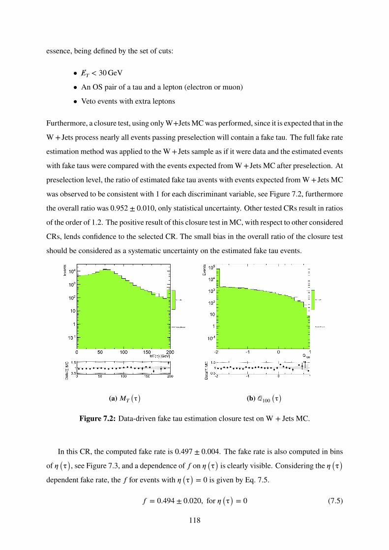
essence, being defined by the set of cuts:

• �E𝑇 < 30GeV

• An OS pair of a tau and a lepton (electron or muon)

• Veto events with extra leptons

Furthermore, a closure test, using onlyW+JetsMCwas performed, since it is expected that in the

W + Jets process nearly all events passing preselection will contain a fake tau. The full fake rate

estimation method was applied to the W + Jets sample as if it were data and the estimated events

with fake taus were compared with the events expected from W + Jets MC after preselection. At

preselection level, the ratio of estimated fake tau avents with events expected from W + Jets MC

was observed to be consistent with 1 for each discriminant variable, see Figure 7.2, furthermore

the overall ratio was 0.952 ± 0.010, only statistical uncertainty. Other tested CRs result in ratios

of the order of 1.2. The positive result of this closure test in MC, with respect to other considered

CRs, lends confidence to the selected CR. The small bias in the overall ratio of the closure test

should be considered as a systematic uncertainty on the estimated fake tau events.

(a) 𝑀𝑇 (τ) (b) 𝒬100 (τ)

Figure 7.2: Data-driven fake tau estimation closure test on W + Jets MC.

In this CR, the computed fake rate is 0.497 ± 0.004. The fake rate is also computed in bins

of 𝜂 (τ), see Figure 7.3, and a dependence of 𝑓 on 𝜂 (τ) is clearly visible. Considering the 𝜂 (τ)dependent fake rate, the 𝑓 for events with 𝜂 (τ) = 0 is given by Eq. 7.5.

𝑓 = 0.494 ± 0.020, for 𝜂 (τ) = 0 (7.5)

118

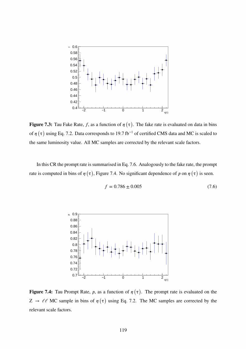
)τ(η2− 1− 0 1 2

f

0.4

0.42

0.44

0.46

0.48

0.5

0.52

0.54

0.56

0.58

0.6

Figure 7.3: Tau Fake Rate, 𝑓, as a function of 𝜂 (τ). The fake rate is evaluated on data in bins

of 𝜂 (τ) using Eq. 7.2. Data corresponds to 19.7 fb−1 of certified CMS data and MC is scaled to

the same luminosity value. All MC samples are corrected by the relevant scale factors.

In this CR the prompt rate is summarised in Eq. 7.6. Analogously to the fake rate, the prompt

rate is computed in bins of 𝜂 (τ), Figure 7.4. No significant dependence of 𝑝 on 𝜂 (τ) is seen.

𝑓 = 0.786 ± 0.005 (7.6)

)τ(η2− 1− 0 1 2

p

0.7

0.72

0.74

0.76

0.78

0.8

0.82

0.84

0.86

0.88

0.9

Figure 7.4: Tau Prompt Rate, 𝑝, as a function of 𝜂 (τ). The prompt rate is evaluated on the

Z → ℓℓ MC sample in bins of 𝜂 (τ) using Eq. 7.2. The MC samples are corrected by the

relevant scale factors.

119

7.2 Fake Tau Estimation

The fakeable object method is used to estimate the fake tau component in this analysis. As pre-

viously mentioned, the method requires the tau identification to be loosened to the loose tau

ID instead of the tight tau ID, i.e. using the byLooseCombinedIsolationDeltaBetaCorr3Hits

discriminator instead of the byTightCombinedIsolationDeltaBetaCorr3Hits discriminator. Ac-

cording to the fakeable object method, the estimated fake tau contribution in a certain SR is

given by Equation 7.7, where 𝑁Fake Taus is the estimated fake tau backgrounds, 𝑁NonTight is the

yield of data events with taus that pass the loose tau identification but do not pass the tight tau

identification and 𝑁Tight is the yield of data events that pass the tight tau identification. This

method can be applied for any given set of cuts, allowing to obtain a data driven prediction of

the fake tau contribution for any of the SR defined in Chapter 6. Equation 7.7 can also be applied

to individual bins in a distribution, allowing to use the 𝜂 (τ) dependent 𝑓 for instance.

𝑁Fake Taus =𝑝 × 𝑓𝑝 − 𝑓

𝑁NonTight −𝑓 × (1 − 𝑝)

𝑝 − 𝑓𝑁Tight (7.7)

Using constant 𝑓 and 𝑝, as measured in Section 7.1, and applying the fakeable object method

(Eq. 7.7) at preselection, a data-driven estimation of the fake tau background for any distribution

is obtained. Figure 7.5, shows the distribution of 𝑝𝑇 (τ) and 𝜂 (τ). The trend of disagreement

between data and the background processes as a function of 𝑝𝑇 (τ), which was previously ob-

served (see Fig. 5.3d), is no longer present. However, a disagreement is observed as a function of

𝜂 (τ), an artefact of using a constant 𝑓. Doing the data driven estimate in bins of 𝜂 (τ), by using

𝑝 = 0.786 ± 0.005 and taking 𝑓 from Figure 7.3 mitigates this disagreement, see the following

section for results. The 𝜂 (τ) dependent fake rate is used in all subsequent sections.

7.3 Event Yields per Signal Region

With the data driven fake tau estimate in place, the background yield at any selection level

is given by the data driven fake tau estimate added to the sum of the prompt component of

the MC processes. At preselection, the data/background ratio is 1.069 ± 0.005, and Table 7.1

summarises the predicted background yields as well as observed data. As expected, the W +Jets

MC component is left with a negligible contribution, with the other processes accounting for

120

(a) 𝑝𝑇 (τ) (b) 𝜂 (τ)

Figure 7.5: 𝑝𝑇 (τ) and 𝜂 (τ) at Preselection using a flat fake rate for the fake tau estimate

the majority of the background, apart from the fake tau component. Fig. 7.6 shows some of the

selection variables at preselection, using the data driven fake tau estimate, which improves the

data/background agreement.

To evaluate the effect of the data driven background estimation, compare Table 7.1 with

Table 5.5 and Fig. 7.6 with Fig. 5.3. The undesirable observation of the disagreement as a

function of 𝑝𝑇 (τ) is no longer present and the overall agreement between data and the estimated

background is significantly improved.

The data driven fake tau method is applied to the three signal regions to obtain the expected

background yield, see Table 7.2. An immediate observation from this table is that there is no

observed excess in data.

121

Table 7.1: Yields after preselection for the fake tau component, using the

data driven method, for the considered MC background processes, for the

total fake tau and MC sum and for data. Data corresponds to 19.7 fb−1 of

certified CMS data and MC is scaled to the same luminosity value. For MC,

only events with prompt taus are considered. The MC samples are corrected

by the relevant scale factors.

Process Yield

Single top 318 ± 12

t t 1647 ± 34

VV/VVV 1426 ± 9

Z → ℓℓ 26 205 ± 179

W + Jets 30 ± 8

Fake Taus 99 354 ± 478

Total Expected 128 980 ± 512

Data 137 902 ± 371

122

lT

p0 20 40 60 80 100

Eve

nts

2−10

1−10

1

10

210

310

410

-1 L=19.7 fb∫=8.0 TeV, s

Single top

tt

VV/VVV

+ Jetsγ

QCD

ll→Z

W + Jets

DDBkg

data

TStauStau_120_20

0 20 40 60 80 100

MC

ΣD

ata/ 0.5

1

1.5

(a) 𝑝𝑇 (ℓ)

lη2− 0 2

Eve

nts

2−10

1−10

1

10

210

310

410

-1 L=19.7 fb∫=8.0 TeV, s

Single top

tt

VV/VVV

+ Jetsγ

QCD

ll→Z

W + Jets

DDBkg

data

TStauStau_120_20

2− 0 2

MC

ΣD

ata/ 0.5

1

1.5

(b) 𝜂 (ℓ)

MT [GeV]0 50 100 150 200

Eve

nts

2−10

1−10

1

10

210

310

410

-1 L=19.7 fb∫=8.0 TeV, s

Single top

tt

VV/VVV

+ Jetsγ

QCD

ll→Z

W + Jets

DDBkg

data

TStauStau_120_20

0 50 100 150 200

MC

ΣD

ata/ 0.5

1

1.5

(c) 𝑀𝑇 (ℓ)

τT

p0 20 40 60 80 100

Eve

nts

1−10

1

10

210

310

410

-1 L=19.7 fb∫=8.0 TeV, s

Single top

tt

VV/VVV

+ Jetsγ

QCD

ll→Z

W + Jets

DDBkg

data

TStauStau_120_20

0 20 40 60 80 100

MC

ΣD

ata/ 0.5

1

1.5

(d) 𝑝𝑇 (τ)

τη2− 0 2

Eve

nts

2−10

1−10

1

10

210

310

410

-1 L=19.7 fb∫=8.0 TeV, s

Single top

tt

VV/VVV

+ Jetsγ

QCD

ll→Z

W + Jets

DDBkg

data

TStauStau_120_20

2− 0 2

MC

ΣD

ata/ 0.5

1

1.5

(e) 𝜂 (τ)

) [GeV]τMT(0 50 100 150 200

Eve

nts

2−10

1−10

1

10

210

310

410

-1 L=19.7 fb∫=8.0 TeV, s

Single top

tt

VV/VVV

+ Jetsγ

QCD

ll→Z

W + Jets

DDBkg

data

TStauStau_120_20

0 50 100 150 200

MC

ΣD

ata/ 0.5

1

1.5

(f) 𝑀𝑇 (τ)

Figure 7.6: Variables after Preselection, the considered background processes are stacked and

compared to data. Data corresponds to 19.7 fb−1 of certified CMS data and background consists

of MC scaled to the same luminosity value for the prompt taus and the above-mentioned data-

driven procedure for the fake taus. All MC samples are corrected by the relevant scale factors.

123

(Lab)τl-

φ∆2− 0 2

Eve

nts

2−10

1−10

1

10

210

310

410

-1 L=19.7 fb∫=8.0 TeV, s

Single top

tt

VV/VVV

+ Jetsγ

QCD

ll→Z

W + Jets

DDBkg

data

TStauStau_120_20

2− 0 2

MC

ΣD

ata/ 0.5

1

1.5

(g) 𝛥𝛷ℓ−τ

MET [GeV]0 50 100 150 200

Eve

nts

2−10

1−10

1

10

210

310

410

510

-1 L=19.7 fb∫=8.0 TeV, s

Single top

tt

VV/VVV

+ Jetsγ

QCD

ll→Z

W + Jets

DDBkg

data

TStauStau_120_20

0 50 100 150 200 M

CΣ

Dat

a/ 0.5

1

1.5

(h) �E𝑇

τl-M0 100 200 300 400 500

Eve

nts

2−10

1−10

1

10

210

310

410

-1 L=19.7 fb∫=8.0 TeV, s

Single top

tt

VV/VVV

+ Jetsγ

QCD

ll→Z

W + Jets

DDBkg

data

TStauStau_120_20

0 100 200 300 400 500

MC

ΣD

ata/ 0.5

1

1.5

(i) 𝑀Inv (ℓ, τ)

[GeV]T2M0 100 200 300 400 500

Eve

nts

1−10

1

10

210

310

410

510

-1 L=19.7 fb∫=8.0 TeV, s

Single top

tt

VV/VVV

+ Jetsγ

QCD

ll→Z

W + Jets

DDBkg

data

TStauStau_120_20

0 100 200 300 400 500

MC

ΣD

ata/ 0.5

1

1.5

(j) 𝑀𝑇 2

Figure 7.6: Variables after Preselection, the considered background processes are stacked and

compared to data. Data corresponds to 19.7 fb−1 of certified CMS data and background consists

of MC scaled to the same luminosity value for the prompt taus and the above-mentioned data-

driven procedure for the fake taus. All MC samples are corrected by the relevant scale factors.

(continued)

124

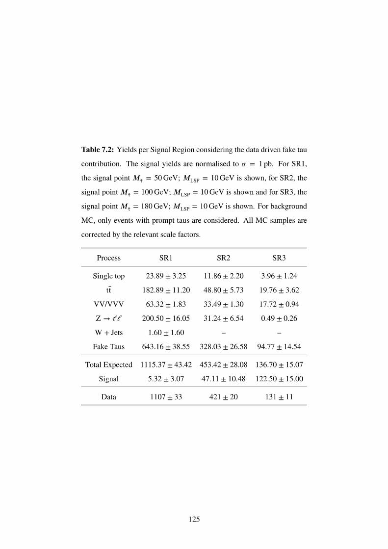
Table 7.2: Yields per Signal Region considering the data driven fake tau

contribution. The signal yields are normalised to 𝜎 = 1 pb. For SR1,

the signal point 𝑀τ = 50GeV; 𝑀LSP = 10GeV is shown, for SR2, the

signal point 𝑀τ = 100GeV; 𝑀LSP = 10GeV is shown and for SR3, the

signal point 𝑀τ = 180GeV; 𝑀LSP = 10GeV is shown. For background

MC, only events with prompt taus are considered. All MC samples are

corrected by the relevant scale factors.

Process SR1 SR2 SR3

Single top 23.89 ± 3.25 11.86 ± 2.20 3.96 ± 1.24

tt 182.89 ± 11.20 48.80 ± 5.73 19.76 ± 3.62

VV/VVV 63.32 ± 1.83 33.49 ± 1.30 17.72 ± 0.94

Z → ℓℓ 200.50 ± 16.05 31.24 ± 6.54 0.49 ± 0.26

W + Jets 1.60 ± 1.60 – –

Fake Taus 643.16 ± 38.55 328.03 ± 26.58 94.77 ± 14.54

Total Expected 1115.37 ± 43.42 453.42 ± 28.08 136.70 ± 15.07

Signal 5.32 ± 3.07 47.11 ± 10.48 122.50 ± 15.00

Data 1107 ± 33 421 ± 20 131 ± 11

125

Chapter 8

Systematic Uncertainties

Estimating the uncertainty of a measurement is an essential part of performing the said measure-

ment. In general, uncertainties can originate from several sources, such as from themeasurement

process itself up to effects of the environment. Uncertainties are split into two types, statistical

uncertainties and systematic uncertainties. Statistical uncertainties result from the statistical

nature of the measurement process and are essentially stochastic in their nature. Systematic

uncertainties result from an effect that consistently affects the result of repeated measurements

which may or may not be known a-priori. In previous chapters all quoted values have been

accompanied by their corresponding statistical uncertainties.

For this analysis, several sources of systematic uncertainty are considered, in particular those

arising from the data driven background estimationmethod and those related to the simulation of

theMC events and the performance of the detector. The effects of the systematic uncertainties on

the yields are estimated by taking the difference between the nominal value of the yield and that

obtained by varying the source of the systematic uncertainty. Several ancillary measurements

are used to calibrate or compute the background and signal yields. The associated uncertainties

constitute the systematic uncertainties for the analysis.

The following sections describe each of the considered systematic uncertainties and their

effects on the yields. The effect of each systematic uncertainty may change depending on the

considered SR.When relevant, the effect of the systematic uncertainty is reported for each signal

region separately. The effect of a systematic uncertainty on the yield can be asymmetric. When

127

the systematic uncertainty is asymmetric, both the up and down variations are reported, with the

up variation above the down variation. Note that, given the data driven background estimation,

the MC is only used to estimate the prompt component of the SM background. Thus, the un-

certainties quoted for the MC SM background processes are only on the prompt subset of those

processes.

8.1 Luminosity

The luminosity is estimated according to the latest recommendations for data acquired in 2012

[97], using the pixel cluster counting method. The MC events are then weighted by the lumi-

nosity estimate so that the MC yield matches the expectation for the given luminosity.

Since the luminosity is a scale applied to MC, the uncertainty on the luminosity translates

directly to the uncertainty on the final yield, for all yields estimated from MC. As a result, the

luminosity systematic uncertainty affects both signal and the background estimated from MC

in the same amount. Note that it does not affect the data driven background estimation. The

uncertainty on the luminosity for the considered data when using the pixel cluster counting

method is 2.6% [98].

8.2 Cross Section

The cross section quantifies the likelihood of an event to occur and is computed within the

framework of a model. The cross section is then used to normalise the expected yield from MC

events.

For the background processes, the cross sections are computed within the SM. The SM has

19 free parameters, 18 of which are measured experimentally and placed into the model in order

to compute the cross sections. The uncertainties on these measured parameters are systematic

uncertainties for the computation of the cross sections. The uncertainties on the cross sections

are taken from the reference standard model cross sections for CMS at 8TeV, [99]. The final

effect on the yields of each process is summarised in Table 8.1.

128

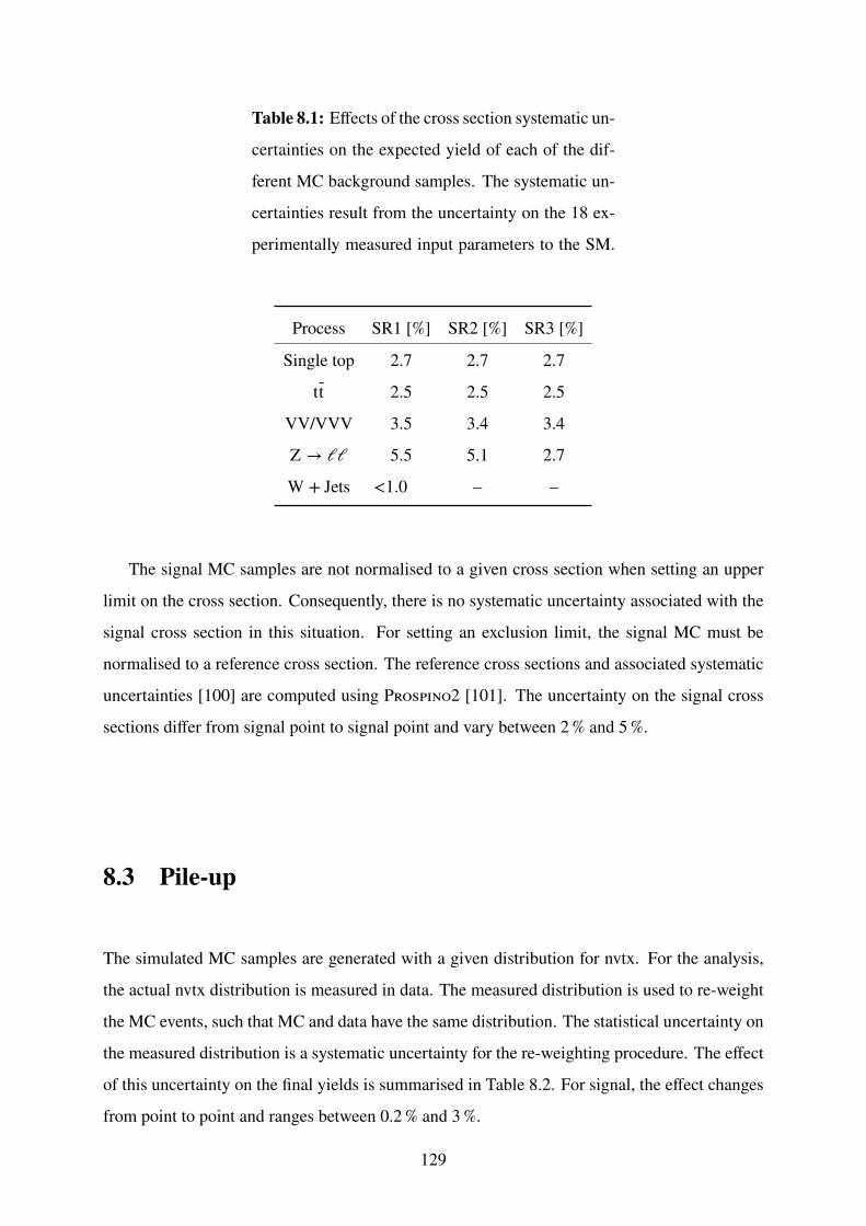
Table 8.1: Effects of the cross section systematic un-

certainties on the expected yield of each of the dif-

ferent MC background samples. The systematic un-

certainties result from the uncertainty on the 18 ex-

perimentally measured input parameters to the SM.

Process SR1 [%] SR2 [%] SR3 [%]

Single top 2.7 2.7 2.7

tt 2.5 2.5 2.5

VV/VVV 3.5 3.4 3.4

Z → ℓℓ 5.5 5.1 2.7

W + Jets <1.0 – –

The signal MC samples are not normalised to a given cross section when setting an upper

limit on the cross section. Consequently, there is no systematic uncertainty associated with the

signal cross section in this situation. For setting an exclusion limit, the signal MC must be

normalised to a reference cross section. The reference cross sections and associated systematic

uncertainties [100] are computed using Prospino2 [101]. The uncertainty on the signal cross

sections differ from signal point to signal point and vary between 2% and 5%.

8.3 Pile-up

The simulated MC samples are generated with a given distribution for nvtx. For the analysis,

the actual nvtx distribution is measured in data. The measured distribution is used to re-weight

the MC events, such that MC and data have the same distribution. The statistical uncertainty on

the measured distribution is a systematic uncertainty for the re-weighting procedure. The effect

of this uncertainty on the final yields is summarised in Table 8.2. For signal, the effect changes

from point to point and ranges between 0.2% and 3%.

129

Table 8.2: Effect of the pile Up systematic uncer-

tainty on the different MC samples and for each SR.


Single top −1.8+2.0

+5.4−4.8

+9.4−8.4

tt < 0.1 +1.6−1.2

+1.3+0.06

VV/VVV +0.8−0.6

+1.0−0.9

+0.9−0.8

Z → ℓℓ −1.8+1.8

−3.2+2.6

−2.2+1.4

W + Jets +5.4−7.2 – –

8.4 PDF

For the simulated MC events, the initial state for the event is chosen according to a Parton Dis-

tribution Function (PDF). The PDFs are measured quantities and have associated uncertainties.

Furthermore, there is a choice of which set of PDFs to use.

To account for the uncertainty on the PDF and for the choice of the chosen PDF, the PDF4LHC

prescription is used [102, 103]. To estimate the effect of this uncertainty, three sets of PDFs are

taken into account, CT10 MSTW2008 and NNPDF23, as well as their uncertainties. For each

event, the weight from each PDF set is used as well as all the uncertainty variations. The largest

deviation is the considered PDF systematic uncertainty. The effect of this uncertainty is sum-

marised in Table 8.3. For signal, the effect changes from point to point and ranges between 0.5%

and 20%.

8.5 Jet Energy Scale and Jet Energy Resolution

Charged hadrons and photons constitute about 85% of the average energy of a jet. The charged

hadron fraction is accurately measured with the tracker, where the tracks give a measurement

of the energy of the particles. The photons are measured in the ECAL. The neutral and charged

hadrons are measured by the HCAL, which is a sampling detector so only a fraction of the de-

posited energy is measured. Furthermore, to reach the HCAL the hadrons must pass through the

130

Table 8.3: Effect of the PDF systematic uncertainty

on the different MC samples and for each SR.


Single top +12.1−13.9

+42.6−47.5

+18.9−18.4

tt +9.5−9.8

+11.1−11.3

+10.1−11.2

VV/VVV +10.2−8.9

+13.7−11.3

+17.7−14.6

Z → ℓℓ +7.8−6.8

+6.9−7.1

+9.4−12.1

W + Jets +31.8−28.2 – –

ECAL, also leaving some energy depositions in it. In order to accurately reconstruct the energy

of a jet, all this information must be correctly taken into account and the non-linearity of the

detector response must be calibrated. To complicate this process, there are the PU interactions,

which provide additional background particles and energy.

To correct for all these effects and reconstruct the jet energy, the set of so-called Jet Energy

Corrections (JEC) are applied to the jets. The JEC are a set of sequential corrections to be

applied to the jets, as a function of the jet properties, and are essentially a scaling of the jet’s

four-momentum, i.e. they are setting the Jet Energy Scale (JES). Each step of the JEC corrects

for a specific effect. Naturally, the corrections are estimated from several measurements, which

have their associated uncertainties, which reflect on the final energy scale of the jets, constituting

the JES uncertainty. The final JES uncertainty is below 3% for all considered jets.

In addition to effects that affect the absolute scale of the jets, some can also affect the resolu-

tion on the transverse momentum of the jets. These effects are also estimated and are introduced

as a systematic uncertainty on the jets, the Jet Energy Resolution (JER) uncertainty. The total

JER uncertainty varies between 2% and 4% in the tracker region and goes up to 10% in the end

caps and HF. An in depth description of the JEC procedure and all associated uncertainties can

be found in [104]. The effect of these uncertainties on this analysis are summarised in Table 8.4

and 8.5. The effect of these uncertainties on signal are typically very low, below 1%, for some

signal points the effect goes up to 6%.

131

Table 8.4: Effect of the jet energy scale systematic

uncertainty on the different MC samples and for each

SR.



+4.1−7.7

+0−11.3

tt −0.9+0.4

+4.0−8.9

+0.2−4.3

VV/VVV +3.2−2.0

+4.0−4.3

+6.4−6.9

Z → ℓℓ +1.2−4.6

+0.4−2.7

+0−0

W + Jets +54.9−0 – –

Table 8.5: Effect of the jet energy resolution system-

atic uncertainty on the different MC samples and for

each SR.


Single top +0.4+3.3

+0+1.4

+0+5.8

tt +0.2+2.8

+3.1−5.2

−1.2−4.9

VV/VVV +1.5+0.2

+1.8−2.3

+3.8−0.6

Z → ℓℓ +2.9−3.9

+2.0−1.4

+0−26.0

W + Jets +0−0 – –

8.6 Lepton Energy Scale

The uncertainty in the strength of the magnetic field, the position of the individual tracking

sensors and of the position of the hits in each sensor translate into an uncertainty of the tracks

reconstructed with those hits. This uncertainty corresponds to an uncertainty of the momentum

of the associated particle, effectively it is an uncertainty on the energy scale of the particle, i.e.

a scaling factor applied to the momentum. Details on the measurement of this uncertainty for

electrons and muons can be found in [82, 85]. For muons the uncertainty is 1%, for electrons

in the barrel region the uncertainty is 2% and for electrons in the endcap regions the uncer-

tainty is 5%. Consequently, in order to evaluate the effect of this uncertainty, the scale of the

objects is varied by the corresponding uncertainty. The effect of this uncertainty is summarised

132

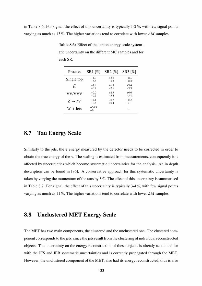
in Table 8.6. For signal, the effect of this uncertainty is typically 1-2%, with few signal points

varying as much as 13%. The higher variations tend to correlate with lower 𝛥𝑀 samples.

Table 8.6: Effect of the lepton energy scale system-

atic uncertainty on the different MC samples and for

each SR.



+3.9−5.3

+11.7−10.0

tt +1.8−0.7

+6.8−7.6

+9.4−3.3

VV/VVV +0.0−0.2

+2.3−3.4

+6.6−3.8

Z → ℓℓ +2.1+0.5

−0.7+0.4

+14.9−0

W + Jets +54.9−0 – –

8.7 Tau Energy Scale

Similarly to the jets, the τ energy measured by the detector needs to be corrected in order to

obtain the true energy of the τ. The scaling is estimated from measurements, consequently it is

affected by uncertainties which become systematic uncertainties for the analysis. An in depth

description can be found in [86]. A conservative approach for this systematic uncertainty is

taken by varying the momentum of the taus by 3%. The effect of this uncertainty is summarised

in Table 8.7. For signal, the effect of this uncertainty is typically 3-4%, with few signal points

varying as much as 11%. The higher variations tend to correlate with lower 𝛥𝑀 samples.

8.8 Unclustered MET Energy Scale

The MET has two main components, the clustered and the unclustered one. The clustered com-

ponent corresponds to the jets, since the jets result from the clustering of individual reconstructed

objects. The uncertainty on the energy reconstruction of these objects is already accounted for

with the JES and JER systematic uncertainties and is correctly propagated through the MET.

However, the unclustered component of the MET, also had its energy reconstructed, thus is also

133

Table 8.7: Effect of the tau energy scale systematic

uncertainty on the different MC samples and for each

SR.



+3.9−1.5

+11.7−11.3

tt +2.8−2.1

+5.2−14.8

+6.6−18.6

VV/VVV +1.7−2.0

+4.6−6.2

+5.2−7.5

Z → ℓℓ +4.1−6.0

+1.7−7.3

+0−0

W + Jets +0−0 – –

affected by an uncertainty. To correctly account for this uncertainty, the MET is separated into

its two components and the unclustered component has its energy varied by 10% [105]. The

effect of this uncertainty is summarised in Table 8.8. For signal, the effect is typically below

6%, with a few low 𝛥𝑀 signal point having values as large as 15%.

Table 8.8: Effect of the unclustered MET energy

scale systematic uncertainty on the different MC

samples and for each SR.



+18.4−31.8

+34.8−18.4

tt +5.4−2.7

+22.9−14.5

+32.2−25.4

VV/VVV +10.6−6.4

+10.0−11.2

+23.6−16.2

Z → ℓℓ −9.8+13.4

−17.3+13.7

+34.6−26.0

W + Jets +54.9−0 – –

8.9 Lepton ID and Isolation

The scale factors that correct for the different efficiency in data and MC of the ID and isolation

requirements are affected by uncertainties, listed in Table 5.3 and Table 5.4. The effect of this

systematic uncertainty is estimated by varying the scale factors by their associated uncertainties.

134

These systematic uncertainties have an effect of 0.1% or lower for all MC samples, signal and

background.

8.10 Tau ID

The tau ID is not required to be corrected by a scale factor. However, this evaluation was based

upon measurements, with associated uncertainties. Consequently, to account for this uncer-

tainty, the weight of the events is varied by 6%. Since all events have a tau, and the variation

of the event weights is a constant number, this systematic uncertainty affects both signal and

background MC by the same fixed amount of 6%.

8.11 Data Driven Method

The fake and prompt rates, measured in Chapter 7, used to estimate the fake tau background

contribution have a non-negligible statistical uncertainty. The statistical uncertainty on the rates

is a source of systematic uncertainty for the data driven background estimation, see Eq. 7.5 and

Eq.7.6 as an example for an event with 𝜂 (τ) = 0. To estimate the effect of this uncertainty, the

fake and prompt rates are independently varied by their statistical uncertainties. The effects of

these uncertainties on the yields of the fake component of each SR are summarised in Table 8.9.

Table 8.9: Effect of the data driven systematic un-

certainties on the estimated fake tau background for

each SR.


Fake Rate +11.1−9.8

+11.4−9.9

+11.4−10.0

Prompt Rate +0.6−0.6

+0.2−0.2

+0.3−0.3

The bias seen in the closure test of the fake tau estimation method should also be present as a

source of systematic uncertainty, an effect of about 5%. However, the uncertainty from the fake

rate has double the value. In order to be economical and conservative, only the uncertainties

from the fake rate and the prompt rate were considered since they provide the needed coverage.

135

Chapter 9

Conclusion

9.1 Final Results

The observed data and predicted SM background yields in each of the three SR are consistent

with each other, see Table 7.2. Thus, no excess of events is observed, as is expected if events

where the stau is produced were to be present. With no hint of discovery, a logical next step is

to set limits on the cross section of the signal process, in order to extract as much information

as possible. Since an SMS scenario was used to generate the signal events, the limit obtained

when using these signal samples is on the 𝜎 × BR of any process consistent with the particles

introduced in the SMS scenario. For this analysis, this corresponds to a limit on the 𝜎 × BR of

any process with stau-like particles which are pair produced and decay to a τ and an undetected

particle.

For the purpose of defining confidence intervals on the 𝜎 × BR, the modified frequentist

approach (CLs) [94, 106] is employed and a simple “cut and count” analysis is performed. The

expected event yield for each mass point is parameterised as Equation 9.1, where 𝑠 (𝑏) is the ex-

pected signal (background) yield for that mass point and is assumed to depend on some nuisance

parameters 𝜃. The signal yield is normalised to a cross section of 1 pb such that the limit on the

signal strength modifier (𝜇) can be interpreted as a limit on 𝜎 × BR.

𝜈 (𝜇, 𝜃) = 𝜇𝑠 (𝜃) + 𝑏 (𝜃) (9.1)

137

The probability to observe 𝑛 events with given an expected yield of 𝜈, is given by:

Poisson (𝑛, 𝜈) = 𝜈𝑛

𝑛!exp (−𝜈) (9.2)

With this parameterisation of the expected event yield, each source of systematic uncertainty

is associated with a nuisance parameter. The nuisance parameters are constrained by auxiliary

measurements, see Chapter 8, that restrict their values with certain confidence intervals. Un-

certainties which correspond to a scaling of the signal and background yields, such as the lu-

minosity uncertainty and efficiency uncertainties, are modelled as a nuisance parameter with a

Log-normal distribution, Equation 9.3. Where 𝑘 is defined as 𝑘 = 1+𝜖, with 𝜖 being the relative

scale of the uncertainty.

𝜌 (𝜃| 𝜃) = 1√2𝜋 ln 𝑘

exp(

−(ln 𝜃/ 𝜃)2

2 (ln 𝑘)2 )1𝜃

(9.3)

Uncertainties that result from counting a number of events (i.e. that are statistical in origin), such

as an uncertainty related to the number of events in a CR, are modelled as a nuisance parameter

with a gamma distribution, Equation 9.4. Where 𝑁 is the observed yield in the CR and 𝑛 is the

expected yield extrapolated with 𝑛 = 𝑁 ⋅ 𝛼.

𝜌 (𝑛|𝑁) = 1𝛼

(𝑛𝛼)

𝑁

𝑁!exp(

𝑛𝛼) (9.4)

The likelihood of observing 𝑛 events (data), considering all of the above, is modelled as:

𝐿 (data|𝜇, 𝜃) = Poisson(𝑛, 𝜈 (𝜇, 𝜃)) ⋅ 𝑝 (𝜃, 𝜃) (9.5)

=(𝜇𝑠 (𝜃) + 𝑏 (𝜃))

𝑛

𝑛!𝑒−(𝜇𝑠(𝜃)+𝑏(𝜃)) ⋅ 𝑝 (

𝜃, 𝜃) (9.6)

Given 𝐿, a test statistic constructed with the profile likelihood ratio is defined as Equation 9.7.

Where 𝜃𝜇 is the set of nuisance parameters which maximise the likelihood function for a fixed

value of 𝜇 and 𝜇 and 𝜃 are the values for the signal strength and nuisance parameters that result

in the global maximum of the likelihood function. The constraint 𝜇 ≤ 𝜇 forces the test statistic

to give one sided confidence intervals while the constraint 𝜇 ≥ 0 has a physical origin, which is

requiring the signal cross-section to be non-negative.

𝑞𝜇 = −2 ln𝐿 (data|𝜇, 𝜃𝜇)

𝐿 (data| 𝜇, 𝜃), constrained by 0 ≤ 𝜇 ≤ 𝜇 (9.7)

138

To establish arbitrary confidence intervals on𝜇 the sampling distribution of 𝑞𝜇, 𝑓 (𝑞𝜇|𝜇′𝑠 + 𝑏),

is needed as a function of 𝜇′. The construction of the sampling distribution can be done by gen-

erating pseudo-data with Monte Carlo techniques or, as an alternative approach, based on an

asymptotic formula for 𝑞𝜇 [95] which is valid in the large sample limit. Given an observed test

statistic, 𝑞𝑜𝑏𝑠𝜇 , the size and the power of the test are defined as:

𝑝𝜇 = 𝑃 (𝑞𝜇 > 𝑞𝑜𝑏𝑠𝜇 |𝜇𝑠 + 𝑏) = ∫

∞

𝑞𝑜𝑏𝑠𝜇

𝑓 (𝑞𝜇|𝜇𝑠 + 𝑏) 𝑑𝑞𝜇 (9.8)

1 − 𝑝𝑏 = 𝑃 (𝑞𝜇 > 𝑞𝑜𝑏𝑠𝜇 |𝑏) = ∫

∞

𝑞𝑜𝑏𝑠𝜇

𝑓 (𝑞𝜇|𝑏) 𝑑𝑞𝜇 (9.9)

The two values are combined to obtain the CLs value for a given 𝜇, Equation 9.10. The

signal strength modifier, 𝜇, is said to be excluded at a confidence level 1 − 𝛼 if CLs is equal to 𝛼.

CLs (𝜇) =𝑝𝜇

1 − 𝑝𝑏(9.10)

The CLs method, as well as other statistical methods, is implemented in the “Higgs Com-

bination Tool” [107], combine for short, developed for the 2012 Higgs boson discovery, which

is the tool that was used for this work. For each signal mass point the expected signal yield,

expected background yields and observed data are obtained and passed to combine for further

processing, accompanied by all the systematic uncertainties, n.b. the background yields and

observed data are the same for all signal mass points within the same SR which is characterised

by a range of 𝛥𝑀.

The result from processing with the combine tool is the CLs upper limit on the 𝜎 × BR at

the 95% confidence level for each signal point. The results were collated and are shown in

Figure 9.1. The expected upper limit on the 𝜎 ×BR is obtained by considering only the expected

background yield and is the result expected in the absence of signal. The observed upper limit

on the 𝜎 ×BR is obtained by taking into account the observed data yield. Given that the expected

background yield and observed data yield are consistent in the three SR, it is not surprising that

the expected and observed upper limits on the 𝜎 × BR are compatible with each other as well.

Since the properties of the signal events are expected to depend primarily on the 𝛥𝑀 (as a first

order effect), it is also expected that the upper limit will also only depend on this parameter. This

effect is clearly seen as bands of similar value travelling from bottom left to top right, where an

upper limit of 𝒪 (10) is seen for low 𝛥𝑀 signal points and the limit decreases as 𝛥𝑀 increases.

139

[GeV]StauM50 100 150 200 250 300 350 400 450 500

[GeV

]LS

PM

0

50

100

150

200

250

300

350

400

450

BR

[pb]

×σ

1−10

1

10

210

310

(a) Expected Limit

(b) Observed Limit

Figure 9.1: Expected and observed upper limit on 𝜎 × BR as a function of 𝑀τ and 𝑀LSP. The

upper limit is computed with the CLs method at 95% confidence level. The expected limit is

the expected result in the absence of signal. The observed limit is the observed upper limit on

𝜎 × BR.

A few of the signal points have no limit set, several factors contributed to this fact. The first

of which is the limited statistics of the simulated MC signal events, which combined with the

selection cuts lead to some of the points not having any events passing the full selection. Other

issues are linked to the combine tool, although not a problem with the tool itself, the algorithm

was not able to converge to a value in a reasonable amount of time. In these situations, no value

for the upper limit is reported.

It is also interesting to interpret the above limits within the pMSSM in the situation where

140

the stau is the Next to Lightest Supersymmetric Particle (NLSP) and the neutralino the LSP. If

the stau is the NLSP, it can only decay to the LSP, consequently the branching ratio, BR, is equal

to 1. In this interpretation the data is modelled with the formula: 𝑁 = 𝐵 + 𝜇′𝑆, where 𝑁 is the

expected yield, 𝐵 is the predicted background yield and 𝑆 the predicted signal yield, correctly

normalised to the theoretical cross section of stau pair production. The upper limits on 𝜎 × BR

are thus reinterpreted into upper limits on the signal strength, 𝜇′. This makes it evident whether

the stau, as the NLSP, can be excluded for any of the signal points.

In order to reinterpret the upper limits on 𝜎 × BR into upper limits on 𝜇, the reference CMS

cross sections [100] for slepton pair production are taken, which depend solely on the stau mass

and do not depend on the assumed SUSY parameters. For each signal point, the upper limit on

𝜎 × BR is then divided by the corresponding reference cross section, resulting in an upper limit

on the signal strength for each signal point, Figure 9.2. It is expected that, in this plot, any point

that has been excluded by these results will have a signal strength below 1. This interpretation

should be taken with care since it is not as model independent as the upper limits on 𝜎 ×BR. In

this interpretation there is the implicit assumption that BR = 1 and that there is no intermediate

new particle whose mass is below 2𝑀τ.

(a) Observed

Figure 9.2: Observed upper limit on the signal strength, 𝜇, as a function of 𝑀τ and 𝑀Neut.

The limit is calculated from the upper limit on the 𝜎 × BR by taking the cross section of stau

production assuming the stau is the NLSP. Points that are excluded with the current dataset,

under this assumption, are expected to have a signal strength below 1.

141

From Figure 9.2 it can be seen that, with the current analysis and processed data, it is not

possible to exclude any of the signal points. The points with the best (i.e. lowest) upper limit

on the signal strength have a value 𝒪 (10) and are located at low 𝑀Neut and with 𝑀τ between

70GeV and 250GeV.

The main result of this work is summarised in Figure 9.1 where limits on the 𝜎 × BR of

any process with stau-like particles which are pair produced and decay to a τ and an undetected

particle are set.

142

9.2 Achievements

Although the work here presented is of the sole responsibility of the author, this work was per-

formed in coordination with the Institute for Research in Fundamental Sciences (IPM) group

of Tehran, where a sustained effort was made to have a common object identification and base

event selection. This effort resulted in the base selection in the publication [33].

Taking into account Figure 9.2 it is clear that within the considered parameter space of

pMSSM, no signal points are excluded. However, it should be noted that at the time of the

writing of this thesis no published results from CMS on the stau production were available.

Thus, the results from Figure 9.1 are considered the main result from this work, whereby limits,

as model independent as possible, are set on the 𝜎 × BR of any process with stau-like particles

which are pair produced and decay to a τ and an undetected particle.

The work for this thesis successfully implemented a new data-driven background estimation

method for fake taus andwas among one of the first analysis in CMS to employ theDeconstructed

𝑀𝑇 variables, despite not being represented in the final set of selected analysis cuts. This work

also successfully implemented an analysis with different selection cuts for different 𝛥𝑀 regions,

thus resulting in a more efficient and targeted selection across the 𝑀τ, 𝑀LSP plane. Furthermore,

the selection was optimised using a FOM procedure, a quantitative procedure with repeatable

results, thus not depending upon qualitative observations.

The results of this work should be compared to the recent results from CMS in publication

[33]. In general, the results of publication [33] show lower upper limits on the cross section of

stau pair production; however it should be noted that the results of this publication use only the

hadronic final state for the stau pair production scenario. The hadronic final state is favoured

by an extremely low W + Jets contribution to the background, resulting in better limits on the

cross section. Thus, the final result is marginally improved with the introduction of the semi-

hadronic channels, explaining why the semi-hadronic final state was not considered for the final

publication [33]. A direct comparison between the work of this thesis and that of the paper

is thus not possible, since the results for the semi-hadronic channel are not shown for the stau

pair production scenario. However, this work is expected to lead to better results in a direct

comparison with the same final state of [33] since a 𝛥𝑀 dependent selection and a robust data-

143

driven background estimation were employed.

It should also be noted that the code for this analysis is embedded within an analysis frame-

work (the 2ℓ2𝜈 framework), the framework provides a common nTuple production code and

object wrapper functions. However, the full analysis code had to be written from scratch, al-

though the process is simplified by the framework. This process was valuable and useful since it

helped provide a firm grasp on the knowledge of how to set up an analysis and provided a view

on the inner workings of cmssw which is many times lost when working with a production ready

analysis where the work focuses on improving the already existing code.

9.3 Future Work

Given the time constraints for the elaboration of this work, not all aspects of the thesis were

explored to their full extent, leaving possible avenues for future work. A first consideration

is the signal MC simulation. For this analysis a sample with 10 000 events per signal mass

point was used, however this proved to be close to the threshold of usability, see Figure 9.1 and

Figure 9.2 where significant statistical fluctuations are evident. A new sample with increased

statistics per mass point would prove useful. If the time dedicated to the simulation of events

can not be increased, this could be reasonably achieved by reducing the range of the signal mass

points where samples are generated. For instance the mass points with 𝑀τ > 300GeV could

most likely be excluded since their cross sections are so low, allowing the remaining mass points

to have increased statistics.

As another example, it was observed that the di-hadronic channel, while more challenging

given the pure hadronic final state, offers a significant improvement on the expected limits, see

[33]. This is a result of the significantly reduced W + Jets background:

• in the semi-leptonic channel, the W + Jets background has proven to be very resilient

to the analysis cuts. The W decays into a real lepton (electron or muon) and a jet fakes a

tau

• in the di-hadronic channel, for W + Jets to pass the event selection two hadronic taus

must be reconstructed. The W decays to a τ in only ~10% of the cases of which only 65%

decay hadronically, in which situation a jet must fake a tau. In all remaining situations,

144

W + Jets events can only pass the selection criteria if two jets fake a tau. In this way, the

W + Jets background is significantly reduced with respect to the semi-leptonic channel

Consequently, the inclusion of the di-hadronic channel in this analysis is expected to bring a

significant improvement to the final results.

The Deconstructed 𝑀𝑇 and the 𝑀SV Fit variables were not present in the final set of analy-

sis cuts. However, it was expected that these variables would be among the most powerful to

discriminate signal from some of the backgrounds. The 𝑀SV Fit variable has a few parameters

to tune its performance, which were not able to be fully explored. For the Deconstructed 𝑀𝑇

variables, a more in depth study of the correlations between the two variables and with �E𝑇 and

𝑀𝑇 is needed to better exploit these variables. For instance, consider Figure 6.10 a non-linear

cut on the (cos𝛷ℓ−�E𝑇, 𝒬80 (ℓ)) plane should perform better than a cut on the 𝒬80 (ℓ)+cos𝛷ℓ−�E𝑇

variable.

During the initial part of the project, the author had the opportunity to work with MVA in the

context of the Higgs analysis. MVAs excel at exploiting differences in correlations of variables

between signal and background. Employing an MVA technique for this analysis would most

likely provide a significant improvement to the final result.

As a final remark, most of this work was developed during the long shutdown of the LHC

and used the latest data available from the CMS collaboration, i.e. the 8TeV data from 2012.

The LHC has since started operation at a new energy and is well on track to recording an even

larger integrated luminosity, updating the analysis to run on the new data is another path for

future development of this work.

145

Bibliography

[1] Vardan Khachatryan et al. “Search for neutral MSSMHiggs bosons decaying to a pair of

tau leptons in pp collisions”. In: JHEP 10 (2014), p. 160. doi: 10.1007/JHEP10(2014)

160. arXiv: 1408.3316 [hep-ex].

[2] S. E. Kuhn. “Observation of a New Type of ’Super’-Symmetry”. In: (2015). arXiv:

1503.09109 [physics.gen-ph].

[3] url: https://en.wikipedia.org/wiki/File:Standard_Model_of_Elementary_

Particles.svg.

[4] D. D. Ryutov. “Using Plasma Physics to Weigh the Photon”. In: Plasma Phys. Control.

Fusion 49 (2007), B429. doi: 10.1088/0741-3335/49/12B/S40.

[5] Serguei Chatrchyan et al. “Observation of a new boson at a mass of 125 GeV with the

CMS experiment at the LHC”. In: Phys. Lett. B716 (2012), pp. 30–61. doi: 10.1016/

j.physletb.2012.08.021. arXiv: 1207.7235 [hep-ex].

[6] Georges Aad et al. “Observation of a new particle in the search for the Standard Model

Higgs boson with the ATLAS detector at the LHC”. In: Phys. Lett. B716 (2012), pp. 1–

29. doi: 10.1016/j.physletb.2012.08.020. arXiv: 1207.7214 [hep-ex].

[7] Serguei Chatrchyan et al. “Evidence for the direct decay of the 125 GeV Higgs boson to

fermions”. In: Nature Phys. 10 (2014), pp. 557–560. doi: 10.1038/nphys3005. arXiv:

1401.6527 [hep-ex].

[8] Georges Aad et al. “Combined Measurement of the Higgs Boson Mass in 𝑝𝑝 Collisions

at √𝑠 = 7 and 8 TeV with the ATLAS and CMS Experiments”. In: Phys. Rev. Lett. 114

(2015), p. 191803. doi: 10.1103/PhysRevLett.114.191803. arXiv: 1503.07589

[hep-ex].

147

http://dx.doi.org/10.1007/JHEP10(2014)160


http://arxiv.org/abs/1408.3316


https://en.wikipedia.org/wiki/File:Standard_Model_of_Elementary_Particles.svg

https://en.wikipedia.org/wiki/File:Standard_Model_of_Elementary_Particles.svg

http://dx.doi.org/10.1088/0741-3335/49/12B/S40

http://dx.doi.org/10.1016/j.physletb.2012.08.021





http://dx.doi.org/10.1038/nphys3005


http://dx.doi.org/10.1103/PhysRevLett.114.191803



[9] The ATLAS and CMS Collaborations. “Measurements of the Higgs boson production

and decay rates and constraints on its couplings from a combined ATLAS and CMS

analysis of the LHC pp collision data at √𝑠 = 7 and 8 TeV”. In: (2015).

[10] S. F. Novaes. “Standard model: An Introduction”. In: Particles and fields. Proceed-

ings, 10th Jorge Andre Swieca Summer School, Sao Paulo, Brazil, February 6-12, 1999.

1999. arXiv: hep-ph/0001283 [hep-ph]. url: http://alice.cern.ch/format/

showfull?sysnb=2173689.

[11] Paul Langacker. “Introduction to the StandardModel and Electroweak Physics”. In: Pro-

ceedings of Theoretical Advanced Study Institute in Elementary Particle Physics on The

dawn of the LHC era (TASI 2008). 2010, pp. 3–48. doi: 10.1142/9789812838360_

0001. arXiv: 0901 . 0241 [hep-ph]. url: https : / / inspirehep . net / record /

810197/files/arXiv:0901.0241.pdf.

[12] S. Dawson. “SUSY and such”. In: NATO Sci. Ser. B 365 (1997), pp. 33–80. doi: 10.

1007/978-1-4615-5963-4_2. arXiv: hep-ph/9612229 [hep-ph].

[13] Howard E. Haber and M. Schmitt. “Supersymmetry”. In: Eur. Phys. J. C15.1-4 (2000),

pp. 817–844. doi: 10.1007/BF02683476.

[14] G. Arnison et al. “Experimental Observation of Lepton Pairs of Invariant Mass Around

95-GeV/c**2 at the CERN SPS Collider”. In: Phys. Lett. B126 (1983), pp. 398–410.

doi: 10.1016/0370-2693(83)90188-0.

[15] G. Arnison et al. “Experimental Observation of Isolated Large Transverse Energy Elec-

trons with Associated Missing Energy at s**(1/2) = 540-GeV”. In: Phys. Lett. B122

(1983). [,611(1983)], pp. 103–116. doi: 10.1016/0370-2693(83)91177-2.

[16] M. Banner et al. “Observation of Single Isolated Electrons of High Transverse Momen-

tum in Events with Missing Transverse Energy at the CERN anti-p p Collider”. In: Phys.

Lett. B122 (1983), pp. 476–485. doi: 10.1016/0370-2693(83)91605-2.

[17] F. J. Hasert et al. “Observation of Neutrino Like Interactions Without Muon Or Electron

in the Gargamelle Neutrino Experiment”. In: Phys. Lett. B46 (1973), pp. 138–140. doi:

10.1016/0370-2693(73)90499-1.

[18] Jean Iliopoulos. “Physics Beyond the Standard Model”. In: (2008). arXiv: 0807.4841

[hep-ph].

148

http://arxiv.org/abs/hep-ph/0001283

http://alice.cern.ch/format/showfull?sysnb=2173689

http://alice.cern.ch/format/showfull?sysnb=2173689

http://dx.doi.org/10.1142/9789812838360_0001

http://dx.doi.org/10.1142/9789812838360_0001


https://inspirehep.net/record/810197/files/arXiv:0901.0241.pdf


http://dx.doi.org/10.1007/978-1-4615-5963-4_2

http://dx.doi.org/10.1007/978-1-4615-5963-4_2


http://dx.doi.org/10.1007/BF02683476

http://dx.doi.org/10.1016/0370-2693(83)90188-0

http://dx.doi.org/10.1016/0370-2693(83)91177-2

http://dx.doi.org/10.1016/0370-2693(83)91605-2

http://dx.doi.org/10.1016/0370-2693(73)90499-1



[19] Max Baak and Roman Kogler. “The global electroweak Standard Model fit after the

Higgs discovery”. In: Proceedings, 48th Rencontres de Moriond on Electroweak In-

teractions and Unified Theories. [,45(2013)]. 2013, pp. 349–358. arXiv: 1306.0571

[hep-ph]. url: https : / / inspirehep . net / record / 1236809 / files / arXiv :

1306.0571.pdf.

[20] Y. Fukuda et al. “Evidence for oscillation of atmospheric neutrinos”. In: Phys. Rev. Lett.

81 (1998), pp. 1562–1567. doi: 10.1103/PhysRevLett.81.1562. arXiv: hep-ex/

9807003 [hep-ex].

[21] M. C. Gonzalez-Garcia and Michele Maltoni. “Phenomenology with Massive Neutri-

nos”. In: Phys. Rept. 460 (2008), pp. 1–129. doi: 10.1016/j.physrep.2007.12.004.

arXiv: 0704.1800 [hep-ph].

[22] P. A. R. Ade et al. “Planck 2015 results. XIII. Cosmological parameters”. In: (2015).

arXiv: 1502.01589 [astro-ph.CO].

[23] H. E. Haber, Gordon L. Kane, and T. Sterling. “The Fermion Mass Scale and Possible

Effects of Higgs Bosons on Experimental Observables”. In: Nucl. Phys. B161 (1979),

p. 493. doi: 10.1016/0550-3213(79)90225-6.

[24] Summary of comparison plots in simplified models spectra for the 8TeV dataset. url:

https://twiki.cern.ch/twiki/bin/view/CMSPublic/SUSYSMSSummaryPlots8TeV

(visited on 03/15/2016).

[25] Guangle Du et al. “Super-Natural MSSM”. In: Phys. Rev. D92.2 (2015), p. 025038. doi:

10.1103/PhysRevD.92.025038. arXiv: 1502.06893 [hep-ph].

[26] Jonathan J. Heckman, Jing Shao, andCumrunVafa. “F-theory and the LHC: Stau Search”.

In: JHEP 09 (2010), p. 020. doi: 10.1007/JHEP09(2010)020. arXiv: 1001.4084

[hep-ph].

[27] Jan Heisig et al. “A survey for low stau yields in theMSSM”. In: JHEP 04 (2014), p. 053.

doi: 10.1007/JHEP04(2014)053. arXiv: 1310.2825 [hep-ph].

[28] Patrick Meade, Nathan Seiberg, and David Shih. “General Gauge Mediation”. In: Prog.

Theor. Phys. Suppl. 177 (2009), pp. 143–158. doi: 10.1143/PTPS.177.143. arXiv:

0801.3278 [hep-ph].

149





http://dx.doi.org/10.1103/PhysRevLett.81.1562

http://arxiv.org/abs/hep-ex/9807003


http://dx.doi.org/10.1016/j.physrep.2007.12.004



http://dx.doi.org/10.1016/0550-3213(79)90225-6

https://twiki.cern.ch/twiki/bin/view/CMSPublic/SUSYSMSSummaryPlots8TeV

http://dx.doi.org/10.1103/PhysRevD.92.025038







http://dx.doi.org/10.1143/PTPS.177.143


[29] John R. Ellis et al. “Calculations of neutralino-stau coannihilation channels and the

cosmologically relevant region of MSSM parameter space”. In: Astropart. Phys. 13

(2000). [Erratum: Astropart. Phys.15,413(2001)], pp. 181–213. doi: 10.1016/S0927-

6505(99)00104-8. arXiv: hep-ph/9905481 [hep-ph].

[30] Jonas M. Lindert, Frank D. Steffen, and Maike K. Trenkel. “Direct stau production at

hadron colliders in cosmologically motivated scenarios”. In: JHEP 08 (2011), p. 151.

doi: 10.1007/JHEP08(2011)151. arXiv: 1106.4005 [hep-ph].

[31] Carola F. Berger et al. “The Number density of a charged relic”. In: JCAP 0810 (2008),

p. 005. doi: 10.1088/1475-7516/2008/10/005. arXiv: 0807.0211 [hep-ph].

[32] Frank Daniel Steffen. “Dark Matter Candidates - Axions, Neutralinos, Gravitinos, and

Axinos”. In: Eur. Phys. J. C59 (2009), pp. 557–588. doi: 10.1140/epjc/s10052-008-

0830-0. arXiv: 0811.3347 [hep-ph].

[33] Vardan Khachatryan et al. Search for electroweak production of charginos in final states

with two 𝜏 leptons in pp collisions at√𝑠 = 8 TeV. Tech. rep. CERN-EP-2016-225. CMS-

SUS-14-022. arXiv:1610.04870. Comments: Submitted to JHEP. Geneva: CERN, Oct.

2016. url: https://cds.cern.ch/record/2225241.

[34] Georges Aad et al. “Search for the direct production of charginos, neutralinos and staus

in final states with at least two hadronically decaying taus and missing transverse mo-

mentum in 𝑝𝑝 collisions at √𝑠 = 8 TeV with the ATLAS detector”. In: JHEP 10 (2014),

p. 096. doi: 10.1007/JHEP10(2014)096. arXiv: 1407.0350 [hep-ex].

[35] Georges Aad et al. “Search for the electroweak production of supersymmetric particles

in √𝑠=8 TeV 𝑝𝑝 collisions with the ATLAS detector”. In: Phys. Rev. D93.5 (2016),

p. 052002. doi: 10.1103/PhysRevD.93.052002. arXiv: 1509.07152 [hep-ex].

[36] G. Abbiendi et al. “Search for anomalous production of dilepton events with missing

transverse momentum in e+ e- collisions at s**(1/2) = 183-Gev to 209-GeV”. In: Eur.

Phys. J. C32 (2004), pp. 453–473. doi: 10.1140/epjc/s2003-01466-y. arXiv: hep-

ex/0309014 [hep-ex].

[37] P. Achard et al. “Search for scalar leptons and scalar quarks at LEP”. In: Phys. Lett.

B580 (2004), pp. 37–49. doi: 10.1016/j.physletb.2003.10.010. arXiv: hep-

ex/0310007 [hep-ex].

150

http://dx.doi.org/10.1016/S0927-6505(99)00104-8

http://dx.doi.org/10.1016/S0927-6505(99)00104-8




http://dx.doi.org/10.1088/1475-7516/2008/10/005


http://dx.doi.org/10.1140/epjc/s10052-008-0830-0



https://cds.cern.ch/record/2225241





http://dx.doi.org/10.1140/epjc/s2003-01466-y






[38] J. Abdallah et al. “Searches for supersymmetric particles in e+ e- collisions up to 208-

GeV and interpretation of the results within the MSSM”. In: Eur. Phys. J. C31 (2003),

pp. 421–479. doi: 10 . 1140 / epjc / s2003 - 01355 - 5. arXiv: hep - ex / 0311019

[hep-ex].

[39] A. Heister et al. “Search for scalar leptons in e+ e- collisions at center-of-mass energies

up to 209-GeV”. In: Phys. Lett. B526 (2002), pp. 206–220. doi: 10 . 1016 / S0370 -

2693(01)01494-0. arXiv: hep-ex/0112011 [hep-ex].

[40] Lyndon Evans and Philip Bryant. “LHC Machine”. In: Journal of Instrumentation 3.08

(2008), S08001. url: http://stacks.iop.org/1748-0221/3/i=08/a=S08001.

[41] Fabienne Marcastel. “CERN’s Accelerator Complex. La chaıne des accélérateurs du

CERN”. In: (Oct. 2013). General Photo. url: http://cds.cern.ch/record/1621583.

[42] url: http://lhc-machine-outreach.web.cern.ch/lhc-machine-outreach/

components/magnets/types_of_magnets.htm.

[43] B. J. Holzer. “Introduction to Transverse Beam Dynamics”. In: Proceedings, CAS -

CERN Accelerator School: Ion Sources. [,21(2014)]. 2014, pp. 27–45. doi: 10.5170/

CERN-2014-005.21,10.5170/CERN-2013-007.27. arXiv: 1404.0923 [physics.acc-ph].

url: https://inspirehep.net/record/1288538/files/arXiv:1404.0923.pdf.

[44] CMS Collaboration. “Detector Drawings”. CMS Collection. Mar. 2012. url: http://

cds.cern.ch/record/1433717.

[45] S. Chatrchyan et al. “The CMS experiment at the CERN LHC”. In: JINST 3 (2008),

S08004. doi: 10.1088/1748-0221/3/08/S08004.

[46] The CMS Collaboration. CMS Physics: Technical Design Report Volume 1: Detector

Performance and Software. Technical Design Report CMS. There is an error on cover

due to a technical problem for some items. Geneva: CERN, 2006. url: https://cds.

cern.ch/record/922757.

[47] Vardan Khachatryan et al. “CMS Tracking Performance Results from early LHC Opera-

tion”. In: Eur. Phys. J. C70 (2010), pp. 1165–1192. doi: 10.1140/epjc/s10052-010-

1491-3. arXiv: 1007.1988 [physics.ins-det].

[48] A. Benaglia. “TheCMSECALperformancewith examples”. In: JINST 9 (2014), p. C02008.

doi: 10.1088/1748-0221/9/02/C02008.

151

http://dx.doi.org/10.1140/epjc/s2003-01355-5



http://dx.doi.org/10.1016/S0370-2693(01)01494-0

http://dx.doi.org/10.1016/S0370-2693(01)01494-0


http://stacks.iop.org/1748-0221/3/i=08/a=S08001

http://cds.cern.ch/record/1621583

http://lhc-machine-outreach.web.cern.ch/lhc-machine-outreach/components/magnets/types_of_magnets.htm

http://lhc-machine-outreach.web.cern.ch/lhc-machine-outreach/components/magnets/types_of_magnets.htm

http://dx.doi.org/10.5170/CERN-2014-005.21, 10.5170/CERN-2013-007.27

http://dx.doi.org/10.5170/CERN-2014-005.21, 10.5170/CERN-2013-007.27





http://dx.doi.org/10.1088/1748-0221/3/08/S08004






http://dx.doi.org/10.1088/1748-0221/9/02/C02008

[49] CMS Collaboration. “ECAL Technical Design Report (TDR) Figures from Chapter 1”.

CMS Collection. Dec. 1997. url: https://cds.cern.ch/record/1327662.

[50] S Chatrchyan et al. “Performance of the CMS Hadron Calorimeter with Cosmic Ray

Muons and LHC Beam Data”. In: JINST 5 (2010), T03012. doi: 10 . 1088 / 1748 -

0221/5/03/T03012. arXiv: 0911.4991 [physics.ins-det].

[51] S Chatrchyan et al. “Precise Mapping of the Magnetic Field in the CMS Barrel Yoke

using Cosmic Rays”. In: JINST 5 (2010), T03021. doi: 10.1088/1748-0221/5/03/

T03021. arXiv: 0910.5530 [physics.ins-det].

[52] V. I. Klyukhin et al. “Measurement of the CMS Magnetic Field”. In: IEEE Trans. Appl.

Supercond. 18 (2008), pp. 395–398. doi: 10.1109/TASC.2008.921242. arXiv: 1110.

0306 [physics.ins-det].

[53] Serguei Chatrchyan et al. “The performance of the CMSmuon detector in proton-proton

collisions at sqrt(s) = 7 TeV at the LHC”. In: JINST 8 (2013), P11002. doi: 10.1088/

1748-0221/8/11/P11002. arXiv: 1306.6905 [physics.ins-det].

[54] S. Dasu et al. “CMS. The TriDAS project. Technical design report, vol. 1: The trigger

systems”. In: (2000).

[55] P. Sphicas. “CMS: The TriDAS project. Technical design report, Vol. 2: Data acquisition

and high-level trigger”. In: (2002).

[56] W. Adam et al. “The CMS high level trigger”. In: Eur. Phys. J.C46 (2006), pp. 605–667.

doi: 10.1140/epjc/s2006-02495-8. arXiv: hep-ex/0512077 [hep-ex].

[57] S. Chatrchyan et al. “The CMS experiment at the CERN LHC”. In: JINST 3 (2008),

S08004. doi: 10.1088/1748-0221/3/08/S08004.

[58] CMS Luminosity Based on Pixel Cluster Counting - Summer 2013 Update. Tech. rep.

CMS-PAS-LUM-13-001. Geneva: CERN, 2013. url: https://cds.cern.ch/record/

1598864.

[59] C. D. Jones et al. “The new CMS event data model and framework”. In: International

Conference on Computing in High Energy and Nuclear Physics (CHEP06). 2006.

[60] Torbjorn Sjostrand, Stephen Mrenna, and Peter Z. Skands. “A Brief Introduction to

PYTHIA 8.1”. In: Comput. Phys. Commun. 178 (2008), pp. 852–867. doi: 10.1016/j.

cpc.2008.01.036. arXiv: 0710.3820 [hep-ph].

152


http://dx.doi.org/10.1088/1748-0221/5/03/T03012

http://dx.doi.org/10.1088/1748-0221/5/03/T03012


http://dx.doi.org/10.1088/1748-0221/5/03/T03021

http://dx.doi.org/10.1088/1748-0221/5/03/T03021


http://dx.doi.org/10.1109/TASC.2008.921242



http://dx.doi.org/10.1088/1748-0221/8/11/P11002

http://dx.doi.org/10.1088/1748-0221/8/11/P11002


http://dx.doi.org/10.1140/epjc/s2006-02495-8


http://dx.doi.org/10.1088/1748-0221/3/08/S08004



http://dx.doi.org/10.1016/j.cpc.2008.01.036

http://dx.doi.org/10.1016/j.cpc.2008.01.036


[61] G. Corcella et al. “HERWIG 6: An Event generator for hadron emission reactions with

interfering gluons (including supersymmetric processes)”. In: JHEP 01 (2001), p. 010.

doi: 10.1088/1126-6708/2001/01/010. arXiv: hep-ph/0011363 [hep-ph].

[62] Z. Was. “TAUOLA the library for tau lepton decay, and KKMC / KORALB / KORALZ

/... status report”. In: Nucl. Phys. Proc. Suppl. 98 (2001). [,96(2000)], pp. 96–102. doi:

10.1016/S0920-5632(01)01200-2. arXiv: hep-ph/0011305 [hep-ph].

[63] Johan Alwall et al. “MadGraph 5 : Going Beyond”. In: JHEP 06 (2011), p. 128. doi:

10.1007/JHEP06(2011)128. arXiv: 1106.0522 [hep-ph].

[64] AndyBuckley et al. “General-purpose event generators for LHCphysics”. In:Phys. Rept.

504 (2011), pp. 145–233. doi: 10.1016/j.physrep.2011.03.005. arXiv: 1101.2599

[hep-ph].

[65] S. Agostinelli et al. “GEANT4: A Simulation toolkit”. In: Nucl. Instrum. Meth. A506

(2003), pp. 250–303. doi: 10.1016/S0168-9002(03)01368-8.

[66] Andrea Giammanco. “The Fast Simulation of the CMS Experiment”. In: J. Phys. Conf.

Ser. 513 (2014), p. 022012. doi: 10.1088/1742-6596/513/2/022012.

[67] S. Cucciarelli et al. “Track reconstruction, primary vertex finding and seed generation

with the pixel detector”. In: (2006).

[68] W. Adam et al. “Track reconstruction in the CMS tracker”. In: (2005).

[69] PaoloAzzurri. “TrackReconstruction Performance in CMS”. In:Nucl. Phys. Proc. Suppl.

197 (2009), pp. 275–278. doi: 10 . 1016 / j . nuclphysbps . 2009 . 10 . 084. arXiv:

0812.5036 [physics.ins-det].

[70] E. Chabanat and N. Estre. “Deterministic annealing for vertex finding at CMS”. In:Com-

puting in high energy physics and nuclear physics. Proceedings, Conference, CHEP’04,

Interlaken, Switzerland, September 27-October 1, 2004. 2005, pp. 287–290. url: http:

//doc.cern.ch/yellowrep/2005/2005-002/p287.pdf.

[71] E. Chabanat and N. Estre. “Deterministic annealing for vertex finding in CMS”. In:

Proceedings of International Conference on Computing in High Energy and Nuclear

Physics (CHEP04). 2004.

[72] T. Speer et al. “Vertex fitting in the CMS tracker”. In: (2006).

153

http://dx.doi.org/10.1088/1126-6708/2001/01/010


http://dx.doi.org/10.1016/S0920-5632(01)01200-2




http://dx.doi.org/10.1016/j.physrep.2011.03.005



http://dx.doi.org/10.1016/S0168-9002(03)01368-8

http://dx.doi.org/10.1088/1742-6596/513/2/022012

http://dx.doi.org/10.1016/j.nuclphysbps.2009.10.084


http://doc.cern.ch/yellowrep/2005/2005-002/p287.pdf

http://doc.cern.ch/yellowrep/2005/2005-002/p287.pdf

[73] “Particle-FlowEvent Reconstruction in CMS and Performance for Jets, Taus, andMET”.

In: (2009).

[74] Florian Beaudette. “The CMS Particle Flow Algorithm”. In: Proceedings, International

Conference on Calorimetry for the High Energy Frontier (CHEF 2013). 2013, pp. 295–

304. arXiv: 1401.8155 [hep-ex]. url: https://inspirehep.net/record/1279774/

files/arXiv:1401.8155.pdf.

[75] Matteo Cacciari, Gavin P. Salam, and Gregory Soyez. “The anti-𝑘𝑇 jet clustering algo-

rithm”. In: JHEP 04 (2008), p. 063. doi: 10.1088/1126-6708/2008/04/063. arXiv:

0802.1189 [hep-ph].

[76] M. Cacciari and G.P. Salam. “Pileup subtraction using jet areas”. In: Phys. Lett. B659

(2008), pp. 119–126. doi: 10.1016/j.physletb.2007.09.077. arXiv: 0707.1378

[hep-ph].

[77] Serguei Chatrchyan et al. “Identification of b-quark jets with the CMS experiment”. In:

JINST 8 (2013), P04013. doi: 10.1088/1748-0221/8/04/P04013. arXiv: 1211.4462

[hep-ex].

[78] CMS. “Performance of tau lepton reconstruction and identification in CMS”. In: JINST

7 (2012), P01001. doi: 10 . 1088 / 1748 - 0221 / 7 / 01 / P01001. arXiv: 1109 . 6034

[physics.ins-det].

[79] Vardan Khachatryan et al. “Performance of the CMS missing transverse momentum

reconstruction in pp data at √𝑠 = 8 TeV”. In: JINST 10.02 (2015), P02006. doi: 10.

1088/1748-0221/10/02/P02006. arXiv: 1411.0511 [physics.ins-det].

[80] Johan Alwall, Philip Schuster, and Natalia Toro. “Simplified Models for a First Char-

acterization of New Physics at the LHC”. In: Phys. Rev. D79 (2009), p. 075020. doi:

10.1103/PhysRevD.79.075020. arXiv: 0810.3921 [hep-ph].

[81] Daniele Alves. “Simplified Models for LHC New Physics Searches”. In: J. Phys. G39

(2012). Ed. by Nima Arkani-Hamed et al., p. 105005. doi: 10.1088/0954-3899/39/

10/105005. arXiv: 1105.2838 [hep-ph].

[82] Vardan Khachatryan et al. “Performance of Electron Reconstruction and Selection with

the CMS Detector in Proton-Proton Collisions at √s = 8 TeV”. In: JINST 10.06 (2015),

P06005. doi: 10.1088/1748-0221/10/06/P06005. arXiv: 1502.02701 [physics.ins-det].

154




http://dx.doi.org/10.1088/1126-6708/2008/04/063





http://dx.doi.org/10.1088/1748-0221/8/04/P04013



http://dx.doi.org/10.1088/1748-0221/7/01/P01001



http://dx.doi.org/10.1088/1748-0221/10/02/P02006

http://dx.doi.org/10.1088/1748-0221/10/02/P02006




http://dx.doi.org/10.1088/0954-3899/39/10/105005

http://dx.doi.org/10.1088/0954-3899/39/10/105005


http://dx.doi.org/10.1088/1748-0221/10/06/P06005


[83] CMS Collaboration. HiggsToTauTau Working Wiki for the 2012 analysis. Twiki Page.

2012. url: https://twiki.cern.ch/twiki/bin/view/CMS/HiggsToTauTauWorkingSummer2013.

[84] “Performance of muon identification in pp collisions at s**0.5 = 7 TeV”. In: (2010).

[85] Serguei Chatrchyan et al. “Performance of CMS muon reconstruction in 𝑝𝑝 collision

events at √𝑠 = 7 TeV”. In: JINST 7 (2012), P10002. doi: 10.1088/1748-0221/7/10/

P10002. arXiv: 1206.4071 [physics.ins-det].

[86] VardanKhachatryan et al. “Reconstruction and identification of τ lepton decays to hadrons

and ν𝜏 at CMS”. In: JINST 11.01 (2016), P01019. doi: 10.1088/1748-0221/11/01/

P01019. arXiv: 1510.07488 [physics.ins-det].

[87] CMS Collaboration. Jet Identification. Twiki Page. 2012. url: https://twiki.cern.

ch/twiki/bin/view/CMS/JetID.

[88] CMS Collaboration. “Pileup Jet Identification”. In: (2013).

[89] Serguei Chatrchyan et al. “Evidence for the 125 GeV Higgs boson decaying to a pair

of 𝜏 leptons”. In: JHEP 05 (2014), p. 104. doi: 10.1007/JHEP05(2014)104. arXiv:

1401.5041 [hep-ex].

[90] C. G. Lester and D. J. Summers. “Measuring masses of semiinvisibly decaying particles

pair produced at hadron colliders”. In: Phys. Lett. B463 (1999), pp. 99–103. doi: 10.

1016/S0370-2693(99)00945-4. arXiv: hep-ph/9906349 [hep-ph].

[91] Alan Barr, Christopher Lester, and P. Stephens. “m(T2): The Truth behind the glamour”.

In: J. Phys.G29 (2003), pp. 2343–2363. doi: 10.1088/0954-3899/29/10/304. arXiv:

hep-ph/0304226 [hep-ph].

[92] Ahmed Ismail et al. “Deconstructed Transverse Mass Variables”. In: Phys. Rev. D91.7

(2015), p. 074002. doi: 10.1103/PhysRevD.91.074002. arXiv: 1409.2868 [hep-ph].

[93] S. I. Bityukov and N. V. Krasnikov. “New physics discovery potential in future experi-

ments”. In: (1999). arXiv: physics/9811025 [physics].

[94] Alexander L. Read. “Presentation of search results: The CL(s) technique”. In: J. Phys.

G28 (2002). [,11(2002)], pp. 2693–2704. doi: 10.1088/0954-3899/28/10/313.

155

https://twiki.cern.ch/twiki/bin/view/CMS/HiggsToTauTauWorkingSummer2013

http://dx.doi.org/10.1088/1748-0221/7/10/P10002

http://dx.doi.org/10.1088/1748-0221/7/10/P10002


http://dx.doi.org/10.1088/1748-0221/11/01/P01019

http://dx.doi.org/10.1088/1748-0221/11/01/P01019


https://twiki.cern.ch/twiki/bin/view/CMS/JetID

https://twiki.cern.ch/twiki/bin/view/CMS/JetID



http://dx.doi.org/10.1016/S0370-2693(99)00945-4

http://dx.doi.org/10.1016/S0370-2693(99)00945-4


http://dx.doi.org/10.1088/0954-3899/29/10/304




http://arxiv.org/abs/physics/9811025

http://dx.doi.org/10.1088/0954-3899/28/10/313

[95] Glen Cowan et al. “Asymptotic formulae for likelihood-based tests of new physics”.

In: Eur. Phys. J. C71 (2011). [Erratum: Eur. Phys. J.C73,2501(2013)], p. 1554. doi:

10.1140/epjc/s10052-011-1554-0,10.1140/epjc/s10052-013-2501-z. arXiv:

1007.1727 [physics.data-an].

[96] CMS Collaboration. Computing the contamination from fakes in leptonic final states.

Tech. rep. 2010. url: http://cms.cern.ch/iCMS/jsp/db_notes/noteInfo.jsp?

cmsnoteid=CMS%20AN-2010/261.

[97] CMS Collaboration. Luminosity Physics Object Group. Twiki Page. 2015. url: https:

//twiki.cern.ch/twiki/bin/viewauth/CMS/TWikiLUM.

[98] CMSCollaboration. “CMSLuminosity Based on Pixel Cluster Counting - Summer 2013

Update”. In: (2013).

[99] F.Wuerthwein. StandardModel Cross Sections for CMS at 8 TeV. Twiki Page. 2015. url:

https://twiki.cern.ch/twiki/bin/viewauth/CMS/StandardModelCrossSectionsat8TeV.

[100] F. Wuerthwein. Slepton pair production cross section as used by CMS in SUS1222.

Twiki Page. 2013. url: https://twiki.cern.ch/twiki/bin/view/LHCPhysics/

SUSYCrossSections8TeVsleptonsleptonCMS.

[101] W. Beenakker, R. Hopker, and M. Spira. “PROSPINO: A Program for the production

of supersymmetric particles in next-to-leading order QCD”. In: (1996). arXiv: hep -

ph/9611232 [hep-ph].

[102] Michiel Botje et al. “The PDF4LHC Working Group Interim Recommendations”. In:

(2011). arXiv: 1101.0538 [hep-ph].

[103] Sergey Alekhin et al. “The PDF4LHC Working Group Interim Report”. In: (2011).

arXiv: 1101.0536 [hep-ph].

[104] Vardan Khachatryan et al. “Jet Energy Scale and Resolution in the CMS Experiment in

pp Collisions at 8 TeV”. In: JINST (Under Review). url: http://cms.cern.ch/iCMS/

jsp/analysis/admin/analysismanagement.jsp?ancode=JME-13-004.

[105] CMSCollaboration.Official Prescription for calculating uncertainties onMissing Trans-

verse Energy. Twiki Page. 2012. url: https://twiki.cern.ch/twiki/bin/view/

CMS/MissingETUncertaintyPrescription.

156

http://dx.doi.org/10.1140/epjc/s10052-011-1554-0, 10.1140/epjc/s10052-013-2501-z


http://cms.cern.ch/iCMS/jsp/db_notes/noteInfo.jsp?cmsnoteid=CMS%20AN-2010/261

http://cms.cern.ch/iCMS/jsp/db_notes/noteInfo.jsp?cmsnoteid=CMS%20AN-2010/261

https://twiki.cern.ch/twiki/bin/viewauth/CMS/TWikiLUM

https://twiki.cern.ch/twiki/bin/viewauth/CMS/TWikiLUM

https://twiki.cern.ch/twiki/bin/viewauth/CMS/StandardModelCrossSectionsat8TeV

https://twiki.cern.ch/twiki/bin/view/LHCPhysics/SUSYCrossSections8TeVsleptonsleptonCMS

https://twiki.cern.ch/twiki/bin/view/LHCPhysics/SUSYCrossSections8TeVsleptonsleptonCMS





http://cms.cern.ch/iCMS/jsp/analysis/admin/analysismanagement.jsp?ancode=JME-13-004

http://cms.cern.ch/iCMS/jsp/analysis/admin/analysismanagement.jsp?ancode=JME-13-004

https://twiki.cern.ch/twiki/bin/view/CMS/MissingETUncertaintyPrescription

https://twiki.cern.ch/twiki/bin/view/CMS/MissingETUncertaintyPrescription

[106] Alexander L. Read. “Modified frequentist analysis of search results (TheCL(s)method)”.

In: Workshop on confidence limits, CERN, Geneva, Switzerland, 17-18 Jan 2000: Pro-

ceedings. 2000, pp. 81–101. url: http://weblib.cern.ch/abstract?CERN-OPEN-

2000-205.

[107] url: https://twiki.cern.ch/twiki/bin/view/CMS/SWGuideHiggsAnalysisCombinedLimit.

157

http://weblib.cern.ch/abstract?CERN-OPEN-2000-205

http://weblib.cern.ch/abstract?CERN-OPEN-2000-205

https://twiki.cern.ch/twiki/bin/view/CMS/SWGuideHiggsAnalysisCombinedLimit

UniversidadedeLisboa InstitutoSuperiorTécnicoCERN-THESIS-2017-060 UniversidadedeLisboa...

Documents

Transcript of UniversidadedeLisboa InstitutoSuperiorTécnicoCERN-THESIS-2017-060 UniversidadedeLisboa...