Universidad Politécnica de Madrid Escuela Técnica Superior de Ingenieros...
252
Universidad Politécnica de Madrid Escuela Técnica Superior de Ingenieros Industriales V ISION -BASED AUTONOMOUS NAVIGATION OF M ULTIROTOR M ICRO A ERIAL V EHICLES Ph.D. Thesis Jesús Pestana Puerta M.Sc. in Automation and Robotics UPM Ingeniero Industrial UPM Master Recherche spécialité ATSI Supélec Ingénieur Supélec 2017
Transcript of Universidad Politécnica de Madrid Escuela Técnica Superior de Ingenieros...

Universidad Politécnica de MadridEscuela Técnica Superior de Ingenieros Industriales
VISION-BASED AUTONOMOUS NAVIGATIONOF MULTIROTOR MICRO AERIAL VEHICLES
Ph.D. Thesis
Jesús Pestana PuertaM.Sc. in Automation and Robotics UPM
Ingeniero Industrial UPMMaster Recherche spécialité ATSI Supélec
Ingénieur Supélec
2017


Departamento de Automática, Ingeniería Eléctrica y Electrónicae Informatica Industrial
Escuela Técnica Superior de Ingenieros IndustrialesUniversidad Politécnica de Madrid
VISION-BASED AUTONOMOUS NAVIGATIONOF MULTIROTOR MICRO AERIAL VEHICLES
A thesis submitted for the degree ofDoctor of Philosophy in Automation and Robotics
Author:Jesús Pestana Puerta
M.Sc. in Automation and Robotics UPMIngeniero Industrial UPM
Master Recherche spécialité ATSI SupélecIngénieur Supélec
Advisors:Dr. Pascual Campoy Cervera
Full Professor UPMDr. Sergio Domínguez Cabrerizo
Professor UPM
Madrid, July 2017


Título:Vision-Based Autonomous Navigation of Multirotor Micro Aerial Vehicles
Autor:Jesús Pestana Puerta
M.Sc. in Automation and Robotics UPMIngeniero Industrial UPM
Master Recherche spécialité ATSI SupélecIngénieur Supélec
Directores:Dr. Pascual Campoy Cervera
Full Professor UPMDr. Sergio Domínguez Cabrerizo
Professor UPM
Tribunal nombrado por el Mgfco. y Excmo. Sr Rector de la Universidad Politécnica de Madrid eldía.........de...................de 2017
TribunalPresidente : ......................................., ............
Secretario : ......................................., ............
Vocal : ......................................., ............
Vocal : ......................................., ............
Vocal : ......................................., ............
Suplente : ......................................., ............
Suplente : ......................................., ............
Realizado el acto de lectura y defensa de la tesis el día ........... de ................ de 2017.
calificación de la Tesis.........................................
El Presidente: Los Vocales:
El Secretario:


A mis padres Domingo y Ana,A mi novia Lola,A Domingo e Irene y Agustín,Al resto de mi familia,Y a mis amigos,
Que me han ayudado a descubrirel valor de continuar explorandoy la satisfacción que proporcionaenfrentarse a nuevos desafíos.
Jesús Pestana Puerta
i


Acknowledgements
I am delighted to express my gratitude for those who have enabled the realization of this PhD thesis.First of all, I am profoundly thankful to my supervisors, professor Pascual Campoy Cervera for hisdirection, scientific insights, innovative ideas and tireless support, and professor Sergio DomínguezCabrerizo for his advice and guidance along the years.
I am grateful to the past and current members of the Computer Vision and Aerial Robotics (CVAR)group, previously Computer Vision Group (CVG), of the Technical University of Madrid (UPM), and itsrelated professors Martin Molina and José María Sebastian; and specifically to my colleagues: IgnacioMellado, José Luis Sánchez López, Dr. Paloma de la Puente, Adrian Carrio, Ramón Suarez, CarlosSampedro, Changhong Fu, Michele Pratusevich, Dr. Iván Fernando Mondragón Bernal, Dr. Jean-FrançoisCollumeau, Dr. Carol Martínez, Dr. Aneesh Chauhan, David Galindo, Juan Carlos Garcia Gordo, Dr.Miguel Olivares and Hriday Bavle among others.
I would like to thank all the members of the Centre for Automation and Robotics (CAR, UPM-CSIC),specially the professors from whom I had the opportunity to learn during my Master’s degree; and themembers, researchers and colleagues of the former Institute of Industrial Automation (IAI, CSIC) withwhom I had the pleasure to work.
It is my pleasure to thank the Autonomous Systems Technologies Research & IntegrationLaboratory (ASTRIL) for hosting my research stay at the Arizona State University (ASU) and speciallyto professor Srikanth Saripalli for his supervision and innovative scientific vision; and my colleagues:Patrick McGarey, Yucong Lin, Aravindhan K. Krishnan and Ben Stinnett.
I am profoundly thankful to the Institute of Computer Graphics and Vision (ICG) of the TechnicalUniversity of Graz (TU Graz) and its members for hosting my research stay and following employmentfor over two years. I would like to thank specifically professors Horst Bischof for providing me withthis opportunity and letting me be part of his scientific endeavors, and Friedrich Fraundorfer for hissupervision, scientific insights, deep research discussions and support. I would also like to thankspecifically my colleagues: Michael Maurer, Dr. Daniel Muschick, Alexander Isop, Thomas Holzmann,Christian Mostegel, Dr. Manuel Hofer, Markus Rumpler, Dr. Gabriele Ermacora, Rudolf Prettenthaler,Horst Possegger, Felix Egger and Devesh Adlakha.
It is my pleasure to thank all the institutions that have provided funding for the realization of this thesisand its related works: the Spanish National Research Council (CSIC) for the pre-doctoral scholarshipthrough the “Junta de Ampliación de Estudios” (JAE, 2010) programme; the UECIMUAVS Project(PIRSES-GA-2010) included in the Marie Curie Program; the Spanish Ministry of Science MICYTDPI2010-20751-C02-01 for project funding; the Austrian Science Fund (FWF) for funding under theprojects V-MAV (I-1537), UFO - Semi-Autonomous Aerial Vehicles for Augmented Reality (I-153644);and the Austrian Research Promotion Agency (FFG) and OMICRON electronics GmbH for fundingthrough the “FreeLine” project (Bridge1/843450).
I am very grateful with my family and close friends for their unconditional support, specially to myparents, my girlfriend and my brothers and their partners.
I also thank all the persons that, while not specifically mentioned, have supported the realization ofthis PhD thesis.

iv ACKNOWLEDGEMENTS

Resumen
El objetivo de esta tesis es conseguir una navegación basada en visión fiable y explorar el potencialde los algoritmos del estado del arte moderno en visión por computador para la robótica aérea, yespecialmente aplicados a drones de tipo multirotor. Dado que las cámaras digitales pueden proveerpotencialmente de una cantidad enorme de información al robot, que son menos costosas que otrasalternativas de sensado y que son muy ligeras; los métodos de estimación basados en visión son muyprometedores para el desarrollo de aplicaciones civiles con drones. La parte principal de esta tesisconsiste en el diseño, la implementación y la evaluación de tres módulos nóveles de propósito generalpara multirotores que utilizan métodos basados en visión para tomar decisiones de navegación.
El primer módulo propuesto es un controlador de navegación para multirotores que fue diseñado paraconseguir un vuelo fiable en entornos sin disponibilidad de señal GPS por medio del uso de la visión porcomputador. Con este objetivo en mente, la estimación de velocidad basada en el flujo óptico del suelofue seleccionada para explorar las implicaciones de la utilización de métodos basados en la visión comoprincipal sistema de medida para la retroalimentación del controlador. Fijar y respetar una limitaciónen la velocidad de navegación fue identificada como una manera fiable de asegurar que la estimación develocidad basada en flujo óptico no falle. El controlador propuesto tiene en cuenta las limitaciones develocidad establecidas por el uso de un método de estimación de la posición basado en odometría visual.Esta capacidad del controlador de respetar una velocidad máxima preconfigurada ha sido utilizada conéxito para realizar investigación en la navegación descentralizada simultánea de múltiples drones.
Una capacidad comúnmente buscada en drones, es la realización de un seguimiento visual y laestabilización del vuelo mientras se adquieren imágenes de un objeto de interés. El segundo módulopropuesto en esta tesis es una arquitectura para el seguimiento en vuelo de objetos. Esta arquitectura fuedesarrollada con el propósito de explorar el potencial de los métodos modernos de seguimiento visualbasados en aprendizaje de máquina, o “machine learning” en inglés. Este tipo de algoritmos tienen comoobjeto determinar la posición de un objeto en el flujo de imágenes. Los métodos de seguimiento visualtradicionales funcionan correctamente en las condiciones para las cuales fueron originalmente diseñados,pero a menudo fallan en situaciones reales. La solución propuesta ha demostrado que los métodos actualesde seguimiento visual basados en aprendizaje de máquina permiten conseguir un seguimiento en vuelofiable de una gran variedad de objetos.
El despliegue rápido de drones autónomos en entornos desconocidos es todavía un problema actualen investigación. Uno de los principales desafíos es el cálculo de trayectorias que permitan unanavegación rápida en dichos entornos. Con este problema en mente, el tercer módulo propuesto permitela generación automática de trayectorias seguras en entornos abarrotados de obstáculos. Este módulo hasido probado utilizando mapas adquiridos en tiempo real a bordo del dron mediante el uso de algoritmosde fotogrametría basados en la visión por computador. Aun usando navegación basada en GPS, mediantela realización de experimentos se ha mostrado que el despliegue rápido de drones es factible inclusoutilizando solo el ordenador y los sensores a bordo del dron.
Parte de los módulos desarrollados han sido liberados en código abierto, contribuyendo al entorno dedesarrollo “Aerostack” de código abierto del CVAR, previamente CVG, (UPM). Los módulos propuestosen esta tesis han sido repetidamente probados con éxito en experimentos fuera del laboratorio y en eventospúblicos, demostrando su fiabilidad y potencial, y promoviendo su evaluación en diferentes escenarios.

Abstract
The aim of this thesis is to attain reliable vision-based navigation and explore the potential of state ofthe art Computer Vision algorithms in Aerial Robotics, and specifically for multirotor drones. Sincedigital cameras can potentially provide a vast amount of information to the robot, are less expensivethan their alternatives and are very lightweight, vision-based estimation methods are very promising forthe development of civilian applications for drones. The main part of this thesis consists on the design,implementation and evaluation of three novel general purpose modules for multirotors that utilize vision-based methods to make navigation decisions.
The first proposed module is a novel multirotor navigation controller that was designed to achievereliable flight in GPS-denied environments by using Computer Vision. With this objective in mind, groundoptical flow speed estimation was selected to explore the implications of using vision-based methodsas the main measurement feedback for the controller. Setting and enforcing a speed limitation duringnavigation was identified as a reliable way to ensure that the optical flow speed estimation method doesnot malfunction. The proposed controller takes into account the speed limitations established by thevision-based odometry estimation method. In addition, by leveraging this capability of the controller toensure navigation respecting the preconfigured maximum speed, it has also been successfully utilized toresearch on decentralized multi-drone navigation.
A common objective for drones is to be able to fly and stabilize looking at and close-by to an objectof interest. The second module proposed in this thesis is a novel vision-based object tracking architecturefor multirotor drones, which was designed to explore the reliability of machine learning based visualtrackers to provide feedback to an object following controller. Visual trackers have the purpose todetermine the position of an object in an image stream and are, therefore, good candidates to achieve thisobjective. However traditional visual tracking methods, though very effective in the specific conditionsfor which they were designed, have the drawback of not generalizing well to the myriad of different visualappearances that real objects exhibit. The proposed architecture has demonstrated that current machinelearning based visual tracking algorithms can reliably provide feedback to a visual servoing controller.
The fast deployment of autonomous drones in unknown environments is still an ongoing researchproblem. One of the main challenges to achieve it is the calculation of trajectories that allow fastnavigation in such areas. With this problem in mind, the third proposed module is a trajectory plannerthat delivers smooth safe trajectories in relatively cluttered environments. The algorithm has been testedexperimentally on maps obtained using an on-board real-time capable Computer Vision mapping method.Although other modules would be needed to decide the exact navigation objectives of the drone, usingthis planner we have shown that it is feasible to deploy drones in unknown outdoors environments, byleveraging the good qualities of maps obtained using state of the art photogrammetry methods.
Part of these modules have been released as open-source, contributing to the CVAR’s, previouslyCVG, (UPM) Open-Source Aerial Robotics Framework “Aerostack”, which main purpose is enablingdrone civilian applications. The proposed modules have been repeatedly evaluated with successfulresults in several out-of-the-lab demonstrations, therefore showing their potential and good qualities.The utilization of the proposed modules in public events has promoted their further testing in differentsettings and applications, e. g. indoors and outdoors flight, narrow corridors, passage through windowsand landing in different conditions.

Acronyms
Following is a description of most commonly acronyms referenced on this work:
API: Application Programming Interface
AR: Augmented Reality
AUVSI: Association for Unmanned Vehicles Systems International
BA: Bundle Adjustment
CEA: Spanish Committee of Automation
CVAR: Computer Vision and Aerial Robotics group (UPM), previously CVG
CVG: Computer Vision Group (UPM)
EKF: Extended Kalman Filter
ERSG: European RPAS Steering Group (ERSG)
EuRoC or EuRoC2014: European Robotics Challenge (2014)
FSM: Finite State-Machine
GCS: Ground Control Station
GPS: Global Positioning System
GS: Ground Station
IBVS: Image Based Visual Servoing
IMAV: International Micro Air Vehicle Conference and Flight Competition
IMU: Inertial Measurement Unit
KF: Kalman Filter
MAV: Micro-Aerial Vehicles
MAVWork: CVG Framework for interfacing with MAVs (2011)
MCL: Monte Carlo Localization
mUAV: Micro Unmanned Aerial Vehicle
NAAs: National Aviation Authorities
LRF: Laser Range Finder
LQR: Linear Quadratic Regulator

x ACRONYMS
PF: Particle Filter
PID: : Proportional-Integral-Derivative controller
QP: Quadratic Programming minimization problem
RC: Radio Controlled or Radio Controller
ROS: Robot Operating System
RPM: Revolutions per Minute
RPA: Remotely Piloted Aircraft
RPAS: Remotely Piloted Aircraft System
R&D: Research and Development
SDK: Software Development Kit
UA: Unmanned Aircraft
UAS: Unmanned Aircraft System
UAV: Unmanned Aerial Vehicle
UVS International: Association for Unmanned Vehicles Systems International
VTOL: Vertical Take-Off and Landing

Contents
Thesis Cover 1
Dedication i
Acknowledgements iii
Resumen v
Abstract vii
Acronyms ix
Contents xi
List of Figures xv
List of Tables xix
List of Algorithms xxi
1 Introduction 11.1 Introduction to UAVs and Multirotors . . . . . . . . . . . . . . . . . . . . . . . . . . . 11.2 Problem Statement . . . . . . . . . . . . . . . . . . . . . . . . . . . . . . . . . . . . . 21.3 Thesis proposal and objectives . . . . . . . . . . . . . . . . . . . . . . . . . . . . . . . 41.4 Dissertation outline . . . . . . . . . . . . . . . . . . . . . . . . . . . . . . . . . . . . . 51.5 Chapter Bibliography . . . . . . . . . . . . . . . . . . . . . . . . . . . . . . . . . . . . 6
2 A General Purpose Configurable Controller for Multirotor MAVs 92.1 Introduction . . . . . . . . . . . . . . . . . . . . . . . . . . . . . . . . . . . . . . . . . 92.2 State of the Art . . . . . . . . . . . . . . . . . . . . . . . . . . . . . . . . . . . . . . . 102.3 Controller Algorithm . . . . . . . . . . . . . . . . . . . . . . . . . . . . . . . . . . . . 12
2.3.1 Control Architecture . . . . . . . . . . . . . . . . . . . . . . . . . . . . . . . . 132.3.2 Multirotor Point Mass Kinematic Model . . . . . . . . . . . . . . . . . . . . . . 142.3.3 Middle-Level Controller . . . . . . . . . . . . . . . . . . . . . . . . . . . . . . 162.3.4 High-Level Controller - State-Machine . . . . . . . . . . . . . . . . . . . . . . 172.3.5 Speed Planner Algorithm . . . . . . . . . . . . . . . . . . . . . . . . . . . . . . 182.3.6 Configurable Parameters Set . . . . . . . . . . . . . . . . . . . . . . . . . . . . 18
xi
xii Contents
2.4 Experimental Results . . . . . . . . . . . . . . . . . . . . . . . . . . . . . . . . . . . . 182.4.1 Videos of Experiments . . . . . . . . . . . . . . . . . . . . . . . . . . . . . . . 192.4.2 Experimental Results - Indoors Flight . . . . . . . . . . . . . . . . . . . . . . . 192.4.3 Experimental Results - Outdoors Flight . . . . . . . . . . . . . . . . . . . . . . 222.4.4 Experimental Results - Flights in IMAV2013 Replica . . . . . . . . . . . . . . . 27
2.5 Future Work . . . . . . . . . . . . . . . . . . . . . . . . . . . . . . . . . . . . . . . . . 372.6 Conclusions . . . . . . . . . . . . . . . . . . . . . . . . . . . . . . . . . . . . . . . . . 372.7 Chapter Bibliography . . . . . . . . . . . . . . . . . . . . . . . . . . . . . . . . . . . . 40
3 Visual Servoing of Arbitrary Objects for Multirotors 433.1 Introduction . . . . . . . . . . . . . . . . . . . . . . . . . . . . . . . . . . . . . . . . . 433.2 State of the Art . . . . . . . . . . . . . . . . . . . . . . . . . . . . . . . . . . . . . . . 443.3 System Description . . . . . . . . . . . . . . . . . . . . . . . . . . . . . . . . . . . . . 46
3.3.1 Image Based Visual Servoing (IBVS) Controller . . . . . . . . . . . . . . . . . 473.3.2 IBVS PD Controller Parameters Breakdown . . . . . . . . . . . . . . . . . . . . 48
3.4 Experiments and Results . . . . . . . . . . . . . . . . . . . . . . . . . . . . . . . . . . 503.4.1 Videos and Dataset of Flight Experiments . . . . . . . . . . . . . . . . . . . . . 513.4.2 Qualitative performance - navigation following suburban house elements . . . . 533.4.3 Qualitative performance - navigation along a street in a suburban area . . . . . . 553.4.4 Quantitative performance - person following without decoupling control heuristics 573.4.5 Quantitative performance - person following with decoupling control heuristics . 60
3.5 Future Work . . . . . . . . . . . . . . . . . . . . . . . . . . . . . . . . . . . . . . . . . 633.6 Conclusions . . . . . . . . . . . . . . . . . . . . . . . . . . . . . . . . . . . . . . . . . 633.7 Chapter Bibliography . . . . . . . . . . . . . . . . . . . . . . . . . . . . . . . . . . . . 66
4 Smooth Trajectory Planning for Multirotors 694.1 Introduction . . . . . . . . . . . . . . . . . . . . . . . . . . . . . . . . . . . . . . . . . 694.2 State of the Art . . . . . . . . . . . . . . . . . . . . . . . . . . . . . . . . . . . . . . . 704.3 Developed Trajectory Planner - Summary . . . . . . . . . . . . . . . . . . . . . . . . . 71
4.3.1 Online Structure-from-Motion (SfM) - Real-Time Mapping . . . . . . . . . . . 724.4 Trajectory Planning - Theoretical Background . . . . . . . . . . . . . . . . . . . . . . . 74
4.4.1 OctoMap - Probabilistic 3D Mapping Framework . . . . . . . . . . . . . . . . . 754.4.2 Dynamic Efficient Obstacle Distance Calculation . . . . . . . . . . . . . . . . . 764.4.3 Probabilistic RoadMap - Planning Algorithm . . . . . . . . . . . . . . . . . . . 764.4.4 Rapidly-Exploring Random Trees - Planning Algorithm . . . . . . . . . . . . . 774.4.5 Utilized open-source libraries . . . . . . . . . . . . . . . . . . . . . . . . . . . 78
4.5 Obstacle-free Smooth Trajectory Planning . . . . . . . . . . . . . . . . . . . . . . . . . 794.5.1 Planner initialization . . . . . . . . . . . . . . . . . . . . . . . . . . . . . . . . 794.5.2 Obstacle-aware Geometric Trajectory Planning . . . . . . . . . . . . . . . . . . 794.5.3 Obstacle-aware Trajectory Shortening and Smoothing . . . . . . . . . . . . . . 804.5.4 Speed, Acceleration and Time-of-passage Planning . . . . . . . . . . . . . . . . 804.5.5 Communication with other modules . . . . . . . . . . . . . . . . . . . . . . . . 864.5.6 Configuration Parameters . . . . . . . . . . . . . . . . . . . . . . . . . . . . . . 87
4.6 Geometric Speed Planner . . . . . . . . . . . . . . . . . . . . . . . . . . . . . . . . . . 874.7 Experimental Results . . . . . . . . . . . . . . . . . . . . . . . . . . . . . . . . . . . . 88
4.7.1 Videos of Experiments . . . . . . . . . . . . . . . . . . . . . . . . . . . . . . . 884.7.2 Experimental Setup . . . . . . . . . . . . . . . . . . . . . . . . . . . . . . . . . 884.7.3 Results in EuRoC 2014 - Challenge 3 - Simulation Contest . . . . . . . . . . . . 894.7.4 Results in 2016 DJI Developer Challenge - Experimental Flights . . . . . . . . . 103
4.8 Future Work . . . . . . . . . . . . . . . . . . . . . . . . . . . . . . . . . . . . . . . . . 1084.9 Conclusions . . . . . . . . . . . . . . . . . . . . . . . . . . . . . . . . . . . . . . . . . 1084.10 Chapter Bibliography . . . . . . . . . . . . . . . . . . . . . . . . . . . . . . . . . . . . 110

Contents xiii
5 Conclusions and Future Work 1135.1 Thesis Contributions . . . . . . . . . . . . . . . . . . . . . . . . . . . . . . . . . . . . 1135.2 Conclusions . . . . . . . . . . . . . . . . . . . . . . . . . . . . . . . . . . . . . . . . . 1185.3 Future Work . . . . . . . . . . . . . . . . . . . . . . . . . . . . . . . . . . . . . . . . . 119
Appendices 121
A Scientific Dissemination 123A.1 Journals . . . . . . . . . . . . . . . . . . . . . . . . . . . . . . . . . . . . . . . . . . . 123A.2 Publications in peer-reviewed conferences . . . . . . . . . . . . . . . . . . . . . . . . . 124A.3 Book Chapters . . . . . . . . . . . . . . . . . . . . . . . . . . . . . . . . . . . . . . . 125A.4 Participation in Conference Workshops . . . . . . . . . . . . . . . . . . . . . . . . . . 125
B UAVs and Multicopters 127B.1 Appendix Bibliography . . . . . . . . . . . . . . . . . . . . . . . . . . . . . . . . . . . 130
C Multirotor Software Interface 131C.1 Introduction . . . . . . . . . . . . . . . . . . . . . . . . . . . . . . . . . . . . . . . . . 131C.2 Robotics Middleware . . . . . . . . . . . . . . . . . . . . . . . . . . . . . . . . . . . . 131C.3 Multirotor Driver . . . . . . . . . . . . . . . . . . . . . . . . . . . . . . . . . . . . . . 132
C.3.1 Notes on the adaptation of the Asctec Pelican to the Multirotor Driver . . . . . . 133C.4 Example Software Architecture (IMAV2012) . . . . . . . . . . . . . . . . . . . . . . . 134C.5 Appendix Bibliography . . . . . . . . . . . . . . . . . . . . . . . . . . . . . . . . . . . 136
D Multirotor dynamics modeling 137D.1 Introduction . . . . . . . . . . . . . . . . . . . . . . . . . . . . . . . . . . . . . . . . . 137D.2 Model based on rigid body dynamics . . . . . . . . . . . . . . . . . . . . . . . . . . . . 137
D.2.1 Brief explanation of the Low-level and Mid-level control of a quadrotor . . . . . 138D.2.2 Shortcomings of the model based on rigid body dynamics . . . . . . . . . . . . 139
D.3 Model based on rigid body dynamics with autopilot . . . . . . . . . . . . . . . . . . . . 140D.4 Simplified model with altitude and yaw hold . . . . . . . . . . . . . . . . . . . . . . . . 142D.5 Complete multirotor simplified model . . . . . . . . . . . . . . . . . . . . . . . . . . . 143
D.5.1 Identification method for this model . . . . . . . . . . . . . . . . . . . . . . . . 145D.5.2 Identification example: Parrot AR Drone with indoors hull . . . . . . . . . . . . 146D.5.3 AR Drone model, comparison with experimental data . . . . . . . . . . . . . . . 149D.5.4 Identification example: Asctec Pelican . . . . . . . . . . . . . . . . . . . . . . . 153
D.6 Conclusions . . . . . . . . . . . . . . . . . . . . . . . . . . . . . . . . . . . . . . . . . 155D.7 Appendix Bibliography . . . . . . . . . . . . . . . . . . . . . . . . . . . . . . . . . . . 156
E An Extended Kalman Filter for Multirotors with Ground Speed Sensing 157E.1 Introduction . . . . . . . . . . . . . . . . . . . . . . . . . . . . . . . . . . . . . . . . . 157E.2 State of the Art . . . . . . . . . . . . . . . . . . . . . . . . . . . . . . . . . . . . . . . 158E.3 Dynamic systems and filtering algorithms . . . . . . . . . . . . . . . . . . . . . . . . . 163
E.3.1 Filtering in State-Observation models . . . . . . . . . . . . . . . . . . . . . . . 164E.4 Kalman filter . . . . . . . . . . . . . . . . . . . . . . . . . . . . . . . . . . . . . . . . 165
E.4.1 The Kalman Filter algorithm . . . . . . . . . . . . . . . . . . . . . . . . . . . 166E.4.2 Extended Kalman Filter . . . . . . . . . . . . . . . . . . . . . . . . . . . . . . 167
E.5 Complete simplified multirotor model, state equations . . . . . . . . . . . . . . . . . . . 168E.6 Testing the EKF on experimental data . . . . . . . . . . . . . . . . . . . . . . . . . . . 169
E.6.1 EKF with odometry measurements . . . . . . . . . . . . . . . . . . . . . . . . . 170E.6.2 EKF with position measurements . . . . . . . . . . . . . . . . . . . . . . . . . 174
E.7 Particle Filter . . . . . . . . . . . . . . . . . . . . . . . . . . . . . . . . . . . . . . . . 178E.7.1 The PF algorithm . . . . . . . . . . . . . . . . . . . . . . . . . . . . . . . . . . 178E.7.2 Testing the PF on experimental data . . . . . . . . . . . . . . . . . . . . . . . . 179
E.8 Conclusions . . . . . . . . . . . . . . . . . . . . . . . . . . . . . . . . . . . . . . . . . 181E.9 Appendix Bibliography . . . . . . . . . . . . . . . . . . . . . . . . . . . . . . . . . . . 182

xiv Contents
F Proportional-Integral-Derivative (PID) controllers 187
G Contributions to the Open-Source Aerial Robotics Framework Aerostack 189
H Utilized Multirotor MAV Platforms 191H.1 AscTec Pelican from Ascending Technologies . . . . . . . . . . . . . . . . . . . . . . . 192
H.1.1 Asctec Pelican Multirotor Experimental Setup - IMAV 2012 . . . . . . . . . . . 193H.1.2 Asctec Pelican Multirotor Experimental Setup - IARC 2014 . . . . . . . . . . . 193
H.2 Parrot AR Drone 1&2 . . . . . . . . . . . . . . . . . . . . . . . . . . . . . . . . . . . . 194H.3 DJI M100 Quadcopter . . . . . . . . . . . . . . . . . . . . . . . . . . . . . . . . . . . 196
H.3.1 DJI M100 Multirotor Experimental Setup - DJIC 2016 . . . . . . . . . . . . . . 196H.4 Appendix Bibliography . . . . . . . . . . . . . . . . . . . . . . . . . . . . . . . . . . . 199
I International Micro Aerial Vehicle Competitions 201I.1 2016 DJI Developer Challenge - DJIC 2016 . . . . . . . . . . . . . . . . . . . . . . . . 202
I.1.1 External Links . . . . . . . . . . . . . . . . . . . . . . . . . . . . . . . . . . . 202I.1.2 Short description . . . . . . . . . . . . . . . . . . . . . . . . . . . . . . . . . . 202I.1.3 Achieved Results . . . . . . . . . . . . . . . . . . . . . . . . . . . . . . . . . . 202
I.2 International Micro Air Vehicle Conference and Flight Competition 2016 - IMAV 2016 . 203I.2.1 External Links . . . . . . . . . . . . . . . . . . . . . . . . . . . . . . . . . . . 203I.2.2 Short description . . . . . . . . . . . . . . . . . . . . . . . . . . . . . . . . . . 203I.2.3 Achieved Results . . . . . . . . . . . . . . . . . . . . . . . . . . . . . . . . . . 203
I.3 European Robotics Challenges 2014 - Simulation Challenge 3 - EuRoC 2014 . . . . . . 204I.3.1 External Links . . . . . . . . . . . . . . . . . . . . . . . . . . . . . . . . . . . 204I.3.2 Short description . . . . . . . . . . . . . . . . . . . . . . . . . . . . . . . . . . 204I.3.3 Achieved Results . . . . . . . . . . . . . . . . . . . . . . . . . . . . . . . . . . 204
I.4 International Aerial Robotics Competition 2014 - Mission 7 - IARC 2014 . . . . . . . . 205I.4.1 External Links . . . . . . . . . . . . . . . . . . . . . . . . . . . . . . . . . . . 205I.4.2 Short description . . . . . . . . . . . . . . . . . . . . . . . . . . . . . . . . . . 205I.4.3 Achieved Results . . . . . . . . . . . . . . . . . . . . . . . . . . . . . . . . . . 205
I.5 International Micro Air Vehicle Conference and Flight Competition 2013 - IMAV 2013 . 206I.5.1 External Links . . . . . . . . . . . . . . . . . . . . . . . . . . . . . . . . . . . 206I.5.2 Short description . . . . . . . . . . . . . . . . . . . . . . . . . . . . . . . . . . 206I.5.3 Achieved Results . . . . . . . . . . . . . . . . . . . . . . . . . . . . . . . . . . 206
I.6 International Micro Air Vehicle Conference and Flight Competition 2012 - IMAV 2012 . 207I.6.1 External Links . . . . . . . . . . . . . . . . . . . . . . . . . . . . . . . . . . . 207I.6.2 Short description . . . . . . . . . . . . . . . . . . . . . . . . . . . . . . . . . . 207I.6.3 Achieved Results . . . . . . . . . . . . . . . . . . . . . . . . . . . . . . . . . . 207
I.7 Contest on Control Engineering 2012 - CEA 2012 . . . . . . . . . . . . . . . . . . . . . 208I.7.1 External Links . . . . . . . . . . . . . . . . . . . . . . . . . . . . . . . . . . . 208I.7.2 Short description . . . . . . . . . . . . . . . . . . . . . . . . . . . . . . . . . . 208I.7.3 Achieved Results . . . . . . . . . . . . . . . . . . . . . . . . . . . . . . . . . . 208
J Other Micro Aerial Vehicle Autonomous Flight Demonstrations 209J.1 Using Trajectory Controller and/or State Estimator . . . . . . . . . . . . . . . . . . . . 210J.2 Using Visual Servoing Architecture . . . . . . . . . . . . . . . . . . . . . . . . . . . . 211J.3 Using Trajectory and Speed Planner . . . . . . . . . . . . . . . . . . . . . . . . . . . . 212
Bibliography 213
List of Figures
2.1 Asctec Pelican quadrotor in the IMAV2012 . . . . . . . . . . . . . . . . . . . . . . . . 102.2 General architecture of the controller . . . . . . . . . . . . . . . . . . . . . . . . . . . . 132.3 Free body diagram of a quadrotor . . . . . . . . . . . . . . . . . . . . . . . . . . . . . 142.4 Mid-level controller architecture, IMAV 2012 . . . . . . . . . . . . . . . . . . . . . . . 162.5 High-level control finite state machine . . . . . . . . . . . . . . . . . . . . . . . . . . . 172.6 Controller, experimental test, vertical eight-shape trajectory . . . . . . . . . . . . . . . . 202.7 Controller, experimental test, horizontal square trajectory . . . . . . . . . . . . . . . . . 202.8 Controller, experimental test, horizontal eight-shape trajectory . . . . . . . . . . . . . . 212.9 Controller, experimental test, horizontal eight-shape trajectory . . . . . . . . . . . . . . 212.10 Controller, outdoors test, pseudo-square trajectory . . . . . . . . . . . . . . . . . . . . . 242.11 Controller, outdoors test, pseudo-hexagon trajectory . . . . . . . . . . . . . . . . . . . . 252.12 Controller, outdoors test, pseudo-octagon trajectory . . . . . . . . . . . . . . . . . . . . 262.13 Flights in IMAV2013 Replica - Summary figure . . . . . . . . . . . . . . . . . . . . . . 272.14 Flights in IMAV2013 Replica - IMAV2013 Coordinate Frames . . . . . . . . . . . . . . 282.15 IMAV2013 Replica Experimental Flight - Overview . . . . . . . . . . . . . . . . . . . . 312.16 IMAV2013 Replica Experimental Flight - Highlights . . . . . . . . . . . . . . . . . . . 322.17 IMAV2013 Replica Experimental Flight - Drift correction . . . . . . . . . . . . . . . . . 332.18 IMAV2013 Replica Experimental Flight - Drone 1 . . . . . . . . . . . . . . . . . . . . . 342.19 IMAV2013 Replica Experimental Flight - Drone 2 . . . . . . . . . . . . . . . . . . . . . 352.20 IMAV2013 Replica Experimental Flight - Drone 3 . . . . . . . . . . . . . . . . . . . . . 36
3.1 Visual Servoing Summary with AR Drone . . . . . . . . . . . . . . . . . . . . . . . . . 443.2 Visual Servoing, main reference frames . . . . . . . . . . . . . . . . . . . . . . . . . . 463.3 Visual Servoing, system overview . . . . . . . . . . . . . . . . . . . . . . . . . . . . . 473.4 Diagram of the Image Based Visual Servoing (IBVS) Controller . . . . . . . . . . . . . 483.5 Visual Servoing, Controller Gains Breakdown . . . . . . . . . . . . . . . . . . . . . . . 493.6 Selection of on-board camera images I . . . . . . . . . . . . . . . . . . . . . . . . . . . 503.7 Selection of on-board camera images II . . . . . . . . . . . . . . . . . . . . . . . . . . 503.8 Selection of on-board camera images - navigation following suburban house elements . . 543.9 Selection of on-board camera images - navigation along a street in a suburban area . . . 553.10 Selection of images - navigation along a street in a suburban area II . . . . . . . . . . . . 563.11 Selection of on-board camera images III . . . . . . . . . . . . . . . . . . . . . . . . . . 573.12 Visual Servoing, test 1, measured and reference values . . . . . . . . . . . . . . . . . . 583.13 Visual Servoing, test 1, controller commands . . . . . . . . . . . . . . . . . . . . . . . 593.14 Selection of on-board camera images IV . . . . . . . . . . . . . . . . . . . . . . . . . . 60
xv

xvi List of Figures
3.15 Visual Servoing, test 2, measured and reference values . . . . . . . . . . . . . . . . . . 613.16 Visual Servoing, test 2, controller commands . . . . . . . . . . . . . . . . . . . . . . . 62
4.1 Simulated outdoor static environment of EuRoC 2014. . . . . . . . . . . . . . . . . . . 714.2 Outdoor map generated using the SfM “Off-board Approach”. . . . . . . . . . . . . . . 724.3 Outdoor map from SfM “Real-Time On-board Approach”. . . . . . . . . . . . . . . . . 734.4 OcTree, data-structure schematic representation . . . . . . . . . . . . . . . . . . . . . . 754.5 Probabilistic roadmap (PRM), motion planning algorithm . . . . . . . . . . . . . . . . . 774.6 Rapidly-exploring random tree (RRT), motion planning algorithm . . . . . . . . . . . . 784.7 Velocity Smoothing - EuRoC2014 - Example Trajectory 1 - Plots . . . . . . . . . . . . . 914.8 Velocity Smoothing - EuRoC2014 - Example Trajectory 7 - Plots . . . . . . . . . . . . . 924.9 Velocity Smoothing - Number of passes - Example Trajectory 7 . . . . . . . . . . . . . 934.10 Trajectory Planner - EuRoC2014 - Example Trajectory 1 - RGB . . . . . . . . . . . . . 944.11 Trajectory Planner - EuRoC2014 - Example Trajectory 1 - Plots . . . . . . . . . . . . . 944.12 Trajectory Planner - EuRoC2014 - Example Trajectory 2 - RGB . . . . . . . . . . . . . 954.13 Trajectory Planner - EuRoC2014 - Example Trajectory 2 - Plots . . . . . . . . . . . . . 954.14 Trajectory Planner - EuRoC2014 - Example Trajectory 3 - RGB . . . . . . . . . . . . . 964.15 Trajectory Planner - EuRoC2014 - Example Trajectory 3 - Plots . . . . . . . . . . . . . 964.16 Trajectory Planner - EuRoC2014 - Example Trajectory 4 - RGB . . . . . . . . . . . . . 974.17 Trajectory Planner - EuRoC2014 - Example Trajectory 4 - Plots . . . . . . . . . . . . . 974.18 Trajectory Planner - EuRoC2014 - Example Trajectory 5 - RGB . . . . . . . . . . . . . 984.19 Trajectory Planner - EuRoC2014 - Example Trajectory 5 - Plots . . . . . . . . . . . . . 984.20 Trajectory Planner - EuRoC2014 - Example Trajectory 6 - RGB . . . . . . . . . . . . . 994.21 Trajectory Planner - EuRoC2014 - Example Trajectory 6 - Plots . . . . . . . . . . . . . 994.22 Trajectory Planner - EuRoC2014 - Example Trajectory 7 - RGB . . . . . . . . . . . . . 1004.23 Trajectory Planner - EuRoC2014 - Example Trajectory 7 - Plots . . . . . . . . . . . . . 1004.24 Trajectory Planner - EuRoC2014 - Example Trajectory 8 - RGB . . . . . . . . . . . . . 1014.25 Trajectory Planner - EuRoC2014 - Example Trajectory 8 - Plots . . . . . . . . . . . . . 1014.26 Trajectory Planner - EuRoC2014 - Example Trajectory 9 - RGB . . . . . . . . . . . . . 1024.27 Trajectory Planner - EuRoC2014 - Example Trajectory 9 - Plots . . . . . . . . . . . . . 1024.28 Trajectory Planner - DJIC2016 - Example Trajectory 1 - RGB . . . . . . . . . . . . . . 1044.29 Trajectory Planner - DJIC2016 - Example Trajectory 1 - Plots . . . . . . . . . . . . . . 1044.30 Trajectory Planner - DJIC2016 - Example Trajectory 2 - RGB . . . . . . . . . . . . . . 1054.31 Trajectory Planner - DJIC2016 - Example Trajectory 2 - Plots . . . . . . . . . . . . . . 1054.32 Trajectory Planner - DJIC2016 - Example Trajectory 3 - RGB . . . . . . . . . . . . . . 1064.33 Trajectory Planner - DJIC2016 - Example Trajectory 3 - Plots . . . . . . . . . . . . . . 1064.34 Trajectory Planner - DJIC2016 - Example Trajectory 4 - RGB . . . . . . . . . . . . . . 1074.35 Trajectory Planner - DJIC2016 - Example Trajectory 4 - Plots . . . . . . . . . . . . . . 107
B.1 Example of fixed-wing UAV. . . . . . . . . . . . . . . . . . . . . . . . . . . . . . . . . 128B.2 Example of multirotor drone. . . . . . . . . . . . . . . . . . . . . . . . . . . . . . . . . 128
C.1 Abstract multirotor representation or Multirotor Driver . . . . . . . . . . . . . . . . . . 132C.2 IMAV2012 software architecture overview. . . . . . . . . . . . . . . . . . . . . . . . . 134
D.1 Free body diagram of a quadrotor . . . . . . . . . . . . . . . . . . . . . . . . . . . . . 138D.2 Rigid body model with autopilot . . . . . . . . . . . . . . . . . . . . . . . . . . . . . . 141D.3 AR Drone black-box model . . . . . . . . . . . . . . . . . . . . . . . . . . . . . . . . . 141D.4 Pelican black-box model as equipped by the CVG_UPM team for the IMAV2012 . . . . 142D.5 Quadrotor 2D simplified model . . . . . . . . . . . . . . . . . . . . . . . . . . . . . . . 143D.6 Complete multirotor simplified model . . . . . . . . . . . . . . . . . . . . . . . . . . . 143D.7 Experimental identification of LTI blocks for the AR Drone, multirotor simplified model 146D.8 Experimental aerodynamic friction data, AR Drone identification . . . . . . . . . . . . . 147D.9 Experimental aerodynamic friction data (2), AR Drone identification . . . . . . . . . . . 147D.10 Experimental aerodynamic friction data (3), AR Drone identification . . . . . . . . . . . 148D.11 Comparison of AR Drone identified model to experimental data, X-Y trajectory . . . . . 149D.12 Comparison of AR Drone identified model to experimental data, speed in body frame . . 150

List of Figures xvii
D.13 Comparison of AR Drone identified model to experimental data, position coordinates . . 151D.14 Comparison of the AR Drone identified model to experimental data, attitude angles . . . 152D.15 Experimentally identified LTI blocks for Asctec Pelican, multirotor simplified model . . 153
E.1 Multirotor complete simplified model . . . . . . . . . . . . . . . . . . . . . . . . . . . 168E.2 EKF performance using odometry data - X-Y trajectory . . . . . . . . . . . . . . . . . . 170E.3 EKF performance using odometry data - speed in the body frame . . . . . . . . . . . . . 171E.4 EKF performance using odometry data - position coordinates . . . . . . . . . . . . . . . 172E.5 EKF performance using odometry data - attitude angle . . . . . . . . . . . . . . . . . . 173E.6 EKF performance using odometry and Vicon data - X-Y trajectory . . . . . . . . . . . . 174E.7 EKF performance using odometry and Vicon data - speed in the body frame . . . . . . . 175E.8 EKF performance using odometry and Vicon data - position coordinates . . . . . . . . . 176E.9 EKF performance using odometry and Vicon data - attitude angles . . . . . . . . . . . . 177E.10 Particle Filter on a real replica of the IMAV 2012 house, autonomy challenge . . . . . . 179E.11 Particle Filter on a real replica of the IMAV 2012 house, autonomy challenge (2) . . . . 180
F.1 Proportional-Integral-Derivative (PID) controller block diagram . . . . . . . . . . . . . 187
H.1 Asctec Pelican quadrotor - CVG-UPM at IARC2014 . . . . . . . . . . . . . . . . . . . 192H.2 Pelican on CVG Framework for interfacing with MAVs . . . . . . . . . . . . . . . . . . 193H.3 Parrot AR Drone 2.0 quadcopter . . . . . . . . . . . . . . . . . . . . . . . . . . . . . . 194H.4 Fully equipped DJI M100 quadcopter . . . . . . . . . . . . . . . . . . . . . . . . . . . 196H.5 Our fully equipped DJI M100 Quadrotor MAV . . . . . . . . . . . . . . . . . . . . . . 197H.6 MAV Hardware - Onboard Computer, Autopilot and GPS Module . . . . . . . . . . . . 197H.7 MAV Hardware - Guidance Sensing System . . . . . . . . . . . . . . . . . . . . . . . . 198H.8 MAV Hardware - Gimbal Camera and Guidance Sensing System . . . . . . . . . . . . . 198


List of Tables
2.1 Controller, results summary of experimental tests (IMAV2012) . . . . . . . . . . . . . . 222.2 Controller, results summary of experimental tests (IMAV2012) . . . . . . . . . . . . . . 222.3 IMAV2013 Replica Experimental Flight - Performance parameters . . . . . . . . . . . . 30
4.1 Trajectory planning and control performance - EuRoC2014 . . . . . . . . . . . . . . . . 904.2 Trajectory planning and control performance - DJIC2016 . . . . . . . . . . . . . . . . . 103
H.1 Asctec Pelican characteristics, from Asctec Pelican website . . . . . . . . . . . . . . . . 192H.2 Parrot AR Drone characteristics . . . . . . . . . . . . . . . . . . . . . . . . . . . . . . 194
xix


List of Algorithms
1 Velocity_Plan_Sweep_Double_Pass(s,r,{t∗i }i ,vdesired ,config
). . . . . . . . . . . . . 82
2 Velocity_Plan_Sweep(vinit ,s,v,r,{t∗i }i ,config
). . . . . . . . . . . . . . . . . . . . . 83
3 Velocity_Max_Direction(d,config) . . . . . . . . . . . . . . . . . . . . . . . . . . . . 834 Acceleration_Max_Direction(d,config) . . . . . . . . . . . . . . . . . . . . . . . . . . 835 Velocity_Smoothing
(s,r,{t∗i }i ,vplan,∆tplan,r
). . . . . . . . . . . . . . . . . . . . . . 87
6 The Monte Carlo Localization algorithm for a robot using a LRF sensor . . . . . . . . . 179
xxi


Chapter 1Introduction
1.1 Introduction to UAVs and Multirotors
The Research and Development (R&D) in the field of Unmanned Aerial Systems is experiencing anincreasing quantity of investment all around the world. Small UAVs are often used as experimental plat-forms to research on state estimation, control, robotic collaboration, etc; since their dynamic maneuveringand natural instability pose important challenges that are not present with other robotic platforms. In ad-dition, the maneuverability of UAVs is combined with a low payload capability, which in turn requires thedevelopment of algorithms with constrained computation requirements. This fact has resulted in manyresearch focused on testing and demonstrating the possibilities of many different sensors on these plat-forms. It is specially remarkable the usage of cameras (Campoy et al., 2009; Y.-C. Liu et al., 2010; P.Liu et al., 2014), since they are very lightweight and consume little power they are a potentially adequatesensor for UAVs. And consequently, small UAVs have been the target platform for the development anddemonstration of very competitive Computer Vision algorithms.
Many of the R&D is being performed by Universities and other Research institutions, but in the pastfew years there has been a growing number of companies selling UAV platforms, and offering civilianapplication services such as 3D reconstruction based mapping and surveying, visual inspection, etc. Thepaper (Pajares, 2015) presents an overview on remote sensing technologies utilized on small UAVS forsurveying. Since there exists a wide range of possible civilian applications to UAVs, there are many stud-ies that can be consulted. It is interesting to compare and see the evolution of the usage of UAVs over theyears. In the late 90s, the usage of UAVs was still too expensive to allow their commercial development,since manned flights were more cost-effective. The only exception was the development of JapaneseUAVs for agriculture applications (Aerosystems, 1999; Van Blyenburgh, 1999). The progressive minia-turization of computers, inertial measurements units and the extended use of GPS have made possible themanufacturing of small drones. A very good example is the toy AR Drone quadrotor, which demonstratesautomatic take-off, hovering and landing capabilities (Bristeau et al., 2011). These factors and others haveallowed the wider set of civilian applications that are possible to perform nowadays (Pajares, 2015), driv-ing many countries around the world to almost simultaneously conceive a legal regulation framework forthese platforms. The regulations are also aiming to address the growing privacy concerns of the general
1

2 1.2. Problem Statement
public, and some research also focuses on how the current legal framework affects UAVs and proposessolutions (Finn et al., 2012). The general time schedule for the deployment of these frameworks can beconsulted in the following document (ERSG, 2013), which mainly concerns the European Union (EU).The United States of America, Canada, Australia, among many other countries; are advancing the imple-mentation of their legal regulation in a similar pace as the EU. With the advent of these necessary legalframeworks, it is expected that UASs will generate a wide range of new commercial applications. Theinterest on these applications is directing part of the research effort to the necessary safety measures to berequired on commercial UAVs such as obstacle detection and avoidance, visual detectability of UAS, safecommunication data-links and related human factors (ERSG, 2013).
The work in this thesis is mainly concerned with multirotors. Although this work may be applicableto various UAV sizes, the conducted experimental works have been performed with multirotors on the0.350 kg to 4.00 kg weight range and with horizontal sizes of approximately 0.450 m to 1.20 m. Based onthese weight and size characteristics, these aircrafts can be currently classified as multirotors of the MicroAerial Vehicle (MAV) category. In general, throughout this text the term MAV can be considered to bereferred to a multirotor drone or UAV.
Considering only civilian applications, UAVs and their related usages are very active fields of researchand development. Considering only small ones, MAVs are aerial data acquisition platforms that can beutilized at a fraction of the cost of any manned counterpart. Furthermore, this reduced cost allows thedevelopment of aerial data gathering solutions for sectors that could not possibly afford to use a mannedhelicopter; effectively opening untapped commercial markets. For instance, this is the case of periodicalsurveying of agriculture crops.
In addition, UAVs, as any other robotic platforms are suitable to be used in tasks termed as “3D”,Dull, Dangerous or Dirty (Welch et al., 2005); or other inaccessible tasks. UAVs can fly for very extendedperiods of time, longer than any human pilot could possible withstand. Additionally, they can be put atrisk, without endangering a human pilot. These are the reasons why they are used as communication relaysin remote locations, for border patrol and control and surveillance applications. UAVs can be equippedwith adequate payloads and be converted into efficient aerial sensing platforms, making them suitable notonly for aerial photography, but for wildlife monitoring, detection of illegal hunting or general (land, airand some sea) surveying applications. The only factors currently impeding the expansion of commercialapplications based on these platforms are the ongoing development of appropriate regulations, and thestill open robotic technical challenges.
1.2 Problem Statement
During the last few years the ongoing trend towards the integration of robotic systems into existingindustrial applications and their utilization in new innovative and well-suited operations is intensifying.Therefore, there exists a big effort towards the vision-based realization of fully autonomous tasks usinglightweight Unmanned Aerial Systems (UAS). The increasing computational power of small computersand the advent of lightweight general-purpose and application-specific sensors and sensing systems isaccelerating the design of lightweight UAS for civilian applications. In order to put this trend into context,the reader may consider the several new products related to the development of lightweight UAS that havebeen released in the last 4 years. Regarding small computing platforms consider, for instance, the powerand weight of the following on-board computers: the Snapdragon Flight (Qualcomm Technologies, Inc.,2015), the Intel Aero (Intel Corporation, 2016a) and the Nvidia Jetson TK1 (Nvidia Corporation, 2014).There exist now several developer drones which ease the design and implementation of new applicationsusing lightweight multirotors. Some examples of them are: the Intel Aero development drone (IntelCorporation, 2016b), the DJI Matrice (DJI - Da-Jiang Innovations Science and Technology Co., Ltd,2015) multirotor series and the Parrot Bebop 2 (Parrot SA, 2014). The following modern vision-basedsensing systems are examples of specialized lightweight sensors for UAVs. The extremely lightweightdepth-sensor RealSense (Intel Corporation, 2014). And the sensing systems that are able to estimate theirpose and perform obstacle sensing using vision-based depth estimation: the DJI Guidance (Zhou et al.,2015) and the Parrot SLAM dunk (Parrot SA, 2016).
Given the increasing interest in utilizing drones for civilian applications were people may be around,there is an interest in achieving drones lightweight enough for them be harmless. In this sense, the leg-islation is heavily rewarding lightweight UAVs, thus motivating the research in vision-based navigation

Chapter 1. Introduction 3
and control, since digital cameras are lightweight and feature a low power consumption. Stabilizing andcontrolling the drone by means of vision-based feedback, odometry (Fraundorfer and Scaramuzza, 2012;Scaramuzza et al., 2011) and localization are important steps in this direction. Vision-based navigationmay enable the drone to navigate in GPS-denied and indoor environments, for instance (Bachrach et al.,2011). The control and pose estimation problems are not independent, since aggressive maneuvers resultin more rapidly changing image streams from the on-board cameras, therefore they can potentially causethe drone to fail to estimate its motion properly. The controller, thus, needs to account for the sensorlimitations and be able to perform smooth navigation at optimal speeds for the on-board sensors to func-tion properly. Thus, the development of novel odometry algorithms that can process very high frame-ratestreams (Forster et al., 2014) is important for UAS to be able to navigate at high speeds in indoor envi-ronments. There are still many challenges for drones to perform vision-based navigate indoors, like badlylit areas, reflective surfaces, moving objects and self-projected shadows and obstacle-avoidance in highlycluttered environments. Another issue are the presence of disturbances such as wind drafts which may beaddressed by means of a better dynamics modeling of the multirotor, specifically identifying the majorcauses contributing to aerodynamic friction in drones (Leishman et al., 2014). In some civilian applica-tions, for drones to be cost effective, it will be necessary to increase the number of drones per operator,and consider multi-drone systems (Ars Electronica Linz Gmbh, 2012; Hörtner et al., 2012), that can besuccessfully flown while performing a task for interest.
A common objective for drones is to be able to fly and stabilize looking at and close-by to an object ofinterest. This kind of application is defined as visual servoing (Corke, 2011), or object following, and it isof great interest for the visual inspection of infrastructure. Drones have a lot of economic potential for thispurpose, as they promise to lower the cost of such necessary operations or even change their implicationsentirely by allowing to inspect big infrastructure, e. g. bridges, without stopping its normal operation.A closely related task is the realization of person following, enabling a drone to take pictures and videoof a person from interesting vantage points, for instance, while practicing sports or while doing tourism.In order to perform the visual servoing operation, the usage of vision-based methods is very promisingsince images contain a lot of information. Algorithms that are able to locate an object in a sequentialimage stream are defined as visual trackers. There exists a diversity of such methods depending ontheir working principle: based on features, direct methods, based on statistical properties of the trackedobject such as color or shape and others (Baker et al., 2004). Some recent research have worked in theimprovement of traditional methods (Possegger et al., 2015), achieving very competitive results. However,setting aside such important works, traditional methods, though very effective in the specific conditionsfor which they were designed, have the drawback of not generalizing well to the myriad of different visualappearances that real objects exhibit. A very important trend in modern visual tracking research focuseson tackling the problem through data driven approaches and machine learning (Kalal et al., 2012). Thesemethods learn a model for the object of interest on-the-fly, thus they can potentially create a model tailoredfor the object of interest and its surrounding environment and arguably that better discriminates betweenboth, thus achieving more reliable tracking.
The autonomous navigation in real-world environments, for the realization of civilian applications ingeneral situations, requires the drone to map the environment and specifically to be able to detect staticand moving obstacles and avoid collisions with them. Since assuming that the drone knows its sur-rounding environment is a big limitation, a common task that needs to be performed by the drone, whilerealizing a task of interest, is the exploration (Fraundorfer, Heng, et al., 2012) of the environment. Duringthis operation, it is required to incrementally build a map, usually named SLAM (Davison et al., 2007),and decide which parts of the space are occupied by obstacles using statistical methods and memory andcomputationally efficient map representations (Hornung et al., 2013). Navigation through cluttered envi-ronments can be performed reactively (Ross et al., 2013) or by calculating collision-free paths based onthe currently mapped obstacles, a problem which is generally defined as trajectory planning (LaValleet al., 2001). The navigation control performs better when following smooth trajectories, allowing fastermotion, and it benefits from faster trajectory generation algorithms, allowing the drone to make fast de-cisions while navigating in cluttered environments; therefore giving rise to different research trends intrajectory planning. Since robots can move and affect which data is going to be gathered for the mappingof the environment, another innovative research trend is acknowledging the inter-dependence in roboticsof exploration, obstacle mapping and trajectory planning.
The scientific community is starting to acknowledge the importance of experiment reproducibility.In Computer Science related fields, the best way to accomplish it is by releasing the source-code as

4 1.3. Thesis proposal and objectives
open-source and sharing the experimental data, so that other researchers can individually confirm theresults of scientific publications and investigate the capabilities of published methods. In robotics thiskind of reproducibility can be achieved at the level of task-specific libraries and modules or at the big-ger scale of general-purpose robotics architectures. Since modularization can ease this process greatly,researchers favor the adoption of common robotics middle-ware frameworks that provide inter-modulecommunication and other features, among which the Robot Operating System (ROS) has achieved thebiggest acceptance (Willow Garage, 2007). Additionally, in the case of drones there exists a number ofopen-hardware and open-source autopilot boards, one particularly favored board is the Pixhawk autopi-lot (Meier et al., 2015). At a bigger scale the Dronecode Project (Linux Foundation, 2014), supported bythe Linux Foundation, seeks to develop an open-source UAV platform for civilian applications.
The necessity of implementing novel and reliable vision-based navigation methods, exploring thecapabilities of state of the art Computer Vision methods and their applicability to Robotics defines theresearch framework from which this thesis has been developed. This thesis has a strong experimentalbasis and the main research problems tackled during its realization have been: vision-based navigation,vision-based object tracking and following, smooth trajectory and speed planning for drones, and theutilization of vision-based acquired maps for the calculation of obstacle-free paths.
1.3 Thesis proposal and objectivesThe main goal of the Computer Vision Group (CVG-UPM) (CVG-UPM, 2012) in the field of aerial
robotics is the use of Unmanned Aerial Vehicles guided and controlled by a computer to perform appli-cations in non-segregated civilian spaces in an autonomous or semi-autonomous fashion; or to developpost-processing algorithms to increase the degree of automation of the subsequent tasks that are to beconducted after inspection works. This PhD thesis aims to improve the state of the art in this growingfield by making contributions to this general proposal considering the following objectives.
• The development of a novel middle-level controller for multirotors. Its main specification is toconsider possible speed limitations established by the sensing capabilities of the on-board sensors.This main objective is further split into the following requirements:
– The controller will have as output a common interface specification for multirotors. Thismodule should enable the MAV to autonomously track position or speed control references.
– The controller needs to be extended to be able to follow a trajectory and be thoroughly de-bugged and tested, so that it can be used in subsequent projects.
– It is also required for the controller to have several configurable parameters so as to be ad-justable to work with different multirotors, sensors and odometry estimation algorithms.
– Building up on the prior requirement, some odometry estimation algorithms may fail to deliverestimates when navigating at inadequate velocities. As an example, in vision-based odometryestimation it becomes increasingly difficult to match image patches or features in subsequentimages, due to a lack of overlap between them, thus, in practice, setting a maximum navigationvelocity. Therefore, the controller, under normal working conditions, should be able to ensurethat the trajectory will be executed at the optimum speed for the on-board sensors to workproperly.
• The development of a novel visual servoing control architecture for arbitrary object following. Themain objective is attaining stable flight against various objects, and to explore the possibility oftracking objects determined by the user on-the-fly. The development of this architecture will allowto understand the feasibility of safely performing the following of arbitrary objects that are specifiedsequentially by an user during flight.
• The development of a novel trajectory planner for multirotors to fly in outdoors cluttered environ-ments. This main objective is further split into the following requirements:
– The algorithm needs to be lightweight enough to be executed on the on-board computer of themultirotor.

Chapter 1. Introduction 5
– The algorithm has to be tested experimentally on maps obtained using real-time capable Com-puter Vision methods.
– It has to work using a commonly accepted map representation in robotics, calculate obstacle-free smooth trajectories when possible at a safe distance from obstacles and provide a speed,acceleration and time-of-passage plans along with the trajectory path.
– It has to be possible to set the maximum desired speed and acceleration for the trajectorycalculation.
– The speed plan should bound the jerk, i. e. the derivative of the acceleration, of the trajectoryso that the multirotor can fly through it using smooth rotations.
• Providing contributions, in the form of tested and working modules, to the general software archi-tecture for UAVs, and specifically for multirotors, named “Aerostack” that is being continuouslydeveloped and improved by the CVAR, previously CVG, (UPM). Aerostack is a multipurpose soft-ware framework that aims to enable MAVs to perform civilian applications. The author has toactively participate in the publication of open-source software for this framework. The contributedmodules to Aerostack need to be, therefore, reusable by others and reconfigurable so that they canbe utilized in tasks related to the main purpose of the module.
In order to ease the diffusion of results, once the previously listed objectives were achieved and tested,the author has actively participated in public flight demonstrations, such as international MAV competi-tions and other events. The participation in such events also showcases the performance and capabilitiesof Aerostack, fosters the research collaboration among team members and colleagues and promotes thefurther testing of the developed modules in different settings and applications, e. g. indoors and outdoorsflight, narrow corridors, passage through windows, landing in different conditions and so on.
1.4 Dissertation outlineThe chapters of this PhD thesis are dedicated to the main contributions of the author to the state of
the art. A general purpose controller for multirotor MAVs, that has been showcased in many public in-ternational MAV competitions, is presented in Chap. 2. An innovative visual servoing architecture formultirotor MAVs that enables them to follow arbitrarily selected objects is presented in Chap. 3. A tra-jectory and speed planner developed to be compatible with the reknown robotics mapping representationOctomap and that has been shown to work using vision-based reconstructed geo-referenced 3D models ispresented in Chap. 4. The multirotor drones utilized in the realization of experiments during the course ofthis thesis are described in Appx. H. The main body of this PhD thesis ends with Chap. 5 that discussesthe thesis contributions, conclusions and future work.
The software modules, developed during this thesis, that have been released as open-source as partof “Aerostack”, a multipurpose software framework for MAVs developed mainly at the CVAR, or CVG,(UPM), are enumerated in Appx. G. They include the controller architectures discussed in Chap. 2 & 3,and a simple kinematics simulator and a state estimator, presented in Appx. E, that are based on the modelpresented in Appx. D.
During the course of this PhD thesis and as part of the collaboration on the development of“Aerostack”, the robotics modules developed by the author have been utilized for the participation inthe International MAV competitions described, and listed with their corresponding achieved results, inAppx. I. These modules have been also showcased in several public events, which are listed in Appx. J.

6 1.5. Chapter Bibliography
1.5 Chapter BibliographyAerosystems, B. (1999). “Civilian applications: the challenges facing the UAV industry”. Air & Space
Europe (cit. on p. 1).Ars Electronica Linz Gmbh (2012). SPAXELS: DRONE SHOWS SINCE 2012. https : / / www .
spaxels.at/. Accessed: 2017-03-19 (cit. on p. 3).Bachrach, A., Prentice, S., He, R., and Roy, N. (2011). “RANGE-Robust autonomous navigation in GPS-
denied environments”. Journal of Field Robotics 28.5, pp. 644–666 (cit. on p. 3).Baker, S. and Matthews, I. (2004). “Lucas-kanade 20 years on: A unifying framework”. International
journal of computer vision 56.3, pp. 221–255 (cit. on p. 3).Bristeau, P.-J., Callou, F., Vissiere, D., Petit, N., et al. (2011). “The navigation and control technology
inside the ar. drone micro uav”. In: 18th IFAC World Congress. Vol. 18, pp. 1477–1484 (cit. on p. 1).Campoy, P., Correa, J. F., Mondragón, I., Martínez, C., Olivares, M., Mejías, L., and Artieda, J. (2009).
“Computer Vision Onboard UAVs for Civilian Tasks”. Journal of Intelligent and Robotic Systems54.1-3, pp. 105–135 (cit. on p. 1).
Corke, P. (2011). Robotics, vision and control: fundamental algorithms in MATLAB. Vol. 73. Springer(cit. on p. 3).
Davison, A. J., Reid, I. D., Molton, N. D., and Stasse, O. (2007). “MonoSLAM: Real-time single cameraSLAM”. IEEE transactions on pattern analysis and machine intelligence 29.6 (cit. on p. 3).
DJI - Da-Jiang Innovations Science and Technology Co., Ltd (2015). DJI Matrice developer drone line.https://www.dji.com/matrice100. Accessed: 2017-03-18 (cit. on p. 2).
ERSG (2013). Roadmap for the integration of civil Remotely - Piloted Aircraft Systems into the EuropeanAviation System. Tech. rep. European RPAS Steering Group (cit. on p. 2).
Finn, R. L. and Wright, D. (2012). “Unmanned aircraft systems: Surveillance, ethics and privacy in civilapplications”. Computer Law & Security Review 28.2, pp. 184–194 (cit. on p. 2).
Forster, C., Pizzoli, M., and Scaramuzza, D. (2014). “SVO: Fast Semi-Direct Monocular Visual Odome-try”. In: IEEE International Conference on Robotics and Automation (ICRA) (cit. on p. 3).
Fraundorfer, F., Heng, L., Honegger, D., Lee, G. H., Meier, L., Tanskanen, P., and Pollefeys, M. (2012).“Vision-based autonomous mapping and exploration using a quadrotor MAV”. In: Intelligent Robotsand Systems (IROS), 2012 IEEE/RSJ International Conference on. IEEE, pp. 4557–4564 (cit. on p. 3).
Fraundorfer, F. and Scaramuzza, D. (2012). “Visual odometry: Part II: Matching, robustness, optimization,and applications”. IEEE Robotics & Automation Magazine 19.2, pp. 78–90 (cit. on p. 3).
Hornung, A., Wurm, K. M., Bennewitz, M., Stachniss, C., and Burgard, W. (2013). “OctoMap: An effi-cient probabilistic 3D mapping framework based on octrees”. Autonomous Robots 34.3, pp. 189–206(cit. on p. 3).
Hörtner, H., Gardiner, M., Haring, R., Lindinger, C., and Berger, F. (2012). “Spaxels, Pixels in Space-ANovel Mode of Spatial Display.” In: International Conference on Signal Processing and MultimediaApplications, SIGMAP, pp. 19–24 (cit. on p. 3).
Intel Corporation (2014). Intel RealSense Developer Kits. https : / / click . intel . com /realsense.html. Accessed: 2017-03-18 (cit. on p. 2).
Intel Corporation (2016a). Intel Aero Compute Board. https://click.intel.com/intel-aero-platform-for-uavs-compute-board.html. Accessed: 2017-03-18 (cit. on p. 2).
Intel Corporation (2016b). Intel Aero Ready to Fly Drone. https://click.intel.com/intel-aero-ready-to-fly-drone.html. Accessed: 2017-03-18 (cit. on p. 2).
Kalal, Z., Mikolajczyk, K., and Matas, J. (2012). “Tracking-Learning-Detection”. IEEE Transactions onPattern Analysis and Machine Intelligence 34.7, pp. 1409–1422 (cit. on p. 3).
LaValle, S. M. and Kuffner, J. J. (2001). “Randomized kinodynamic planning”. The International Journalof Robotics Research 20.5, pp. 378–400 (cit. on p. 3).
Leishman, R. C., Macdonald, J., Beard, R. W., and McLain, T. W. (2014). “Quadrotors and accelerom-eters: State estimation with an improved dynamic model”. Control Systems, IEEE 34.1, pp. 28–41(cit. on p. 3).
Linux Foundation (2014). Dronecode Project. https://www.dronecode.org/about/. Ac-cessed: 2017-03-18 (cit. on p. 4).
Liu, Y.-C. and Dai, Q.-h. (2010). “A survey of computer vision applied in aerial robotic vehicles”. In:Optics Photonics and Energy Engineering (OPEE), 2010 International Conference on. Vol. 1. IEEE,pp. 277–280 (cit. on p. 1).

Chapter 1. Introduction 7
Liu, P., Chen, A. Y., Huang, Y.-N., Han, J.-Y., Lai, J.-S., Kang, S.-C., Wu, T.-H., Wen, M.-C., and Tsai,M.-H. (2014). “A review of rotorcraft Unmanned Aerial Vehicle (UAV) developments and applicationsin civil engineering”. SMART STRUCTURES AND SYSTEMS 13.6, pp. 1065–1094 (cit. on p. 1).
Meier, L., Honegger, D., and Pollefeys, M. (2015). “PX4: A node-based multithreaded open sourcerobotics framework for deeply embedded platforms”. In: Robotics and Automation (ICRA), 2015 IEEEInternational Conference on. IEEE, pp. 6235–6240 (cit. on p. 4).
Nvidia Corporation (2014). NVIDIA Jetson TK1 developer kit. https : / / www . nvidia . com /object/jetson-tk1-embedded-dev-kit.html. Accessed: 2017-03-18 (cit. on p. 2).
Pajares, G. (2015). “Overview and Current Status of Remote Sensing Applications Based on UnmannedAerial Vehicles (UAVs)”. Photogrammetric Engineering & Remote Sensing 81.4, pp. 281–330 (cit. onp. 1).
Parrot SA (2014). Parrot BEBOP 2. https://www.parrot.com/us/Drones/Parrot-bebop-2. Accessed: 2017-03-18 (cit. on p. 2).
Parrot SA (2016). Parrot S.L.A.M. dunk. https : / / www . parrot . com / us / business -solutions/parrot-slamdunk. Accessed: 2017-03-14 (cit. on p. 2).
Possegger, H., Mauthner, T., and Bischof, H. (2015). “In defense of color-based model-free tracking”. In:Proceedings of the IEEE Conference on Computer Vision and Pattern Recognition, pp. 2113–2120(cit. on p. 3).
Qualcomm Technologies, Inc. (2015). Snapdragon Flight Kit. https://developer.qualcomm.com/hardware/snapdragon-flight. Accessed: 2017-03-18 (cit. on p. 2).
Willow Garage, S. A. I. L. (2007). Robot Operating System (ROS). http://www.ros.org/wiki/(cit. on p. 4).
Ross, S., Melik-Barkhudarov, N., Shankar, K. S., Wendel, A., Dey, D., Bagnell, J. A., and Hebert, M.(2013). “Learning monocular reactive uav control in cluttered natural environments”. In: Roboticsand Automation (ICRA), 2013 IEEE International Conference on. IEEE, pp. 1765–1772 (cit. on p. 3).
Scaramuzza, D. and Fraundorfer, F. (2011). “Visual odometry [tutorial]”. IEEE robotics & automationmagazine 18.4, pp. 80–92 (cit. on p. 3).
Van Blyenburgh, P. (1999). “UAVs: an overview”. Air & Space Europe 1.5, pp. 43–47 (cit. on p. 1).CVG-UPM (2012). Universidad Politécnica de Madrid. Computer Vision Group. Vision for UAV Project.
http://www.vision4uav.com (cit. on p. 4).Welch, G. and Bishop, G. (2005). European Civil Unmanned Air Vehicle Roadmap, Volume 3 Strategic
Research Agenda. Tech. rep. European Civil UAV FP5 R&D Program Members (cit. on p. 2).Zhou, G., Fang, L., Tang, K., Zhang, H., Wang, K., and Yang, K. (2015). “Guidance: A visual sensing
platform for robotic applications”. In: IEEE Conference on Computer Vision and Pattern RecognitionWorkshops, 2015 IEEE CVPR Workshop, pp. 9–14 (cit. on p. 2).


Chapter 2A General Purpose ConfigurableController for Multirotor MAVs
2.1 IntroductionThe final objective of robot applications is for the robot to perform some useful task. The problem of
making an autonomous or semi-autonomous robot perform a task is hard and is realized by a combinationof control, odometry, state estimation and planning algorithms. Planning algorithms have to decide asuccession of steps that leads to the accomplishment of the required objectives. They require to approachthe problem in a friendly set of coordinates, usually related to position coordinates. They may also workwith speed coordinates, but only to optimize certain specifications of the task, and the planning problemusually does not output actuator/engine commands. For instance, if an application requires a quadrotor toapproach multiple points of interest to send video and images to a ground station, the common solution isto approach the problem in position coordinates where static obstacles are defined. Another aspect is thatthe task planner has to assume that the multirotor will be stabilized automatically, and that it will followcommands in position coordinates.
These and other issues are solved by adding interface layers between the multirotor and the taskplanner. In the case of multirotors, the main two problems that have to be addressed are:
• The estimation problem: both the planning algorithm and the controller require an estimation of thestate of the quadrotor. For example the task scheduler, that ensures that the steps specified by theplanning algorithm are being accomplished, will need feedback to determine the accomplishmentof the successive mission objectives. The estimation problem has been described and discussed inAppx. E.
• The stabilization of the vehicle and the capacity to follow paths and position commands are solvedusing ‘controllers’. Controllers are automation algorithms that ultimately generate the commandsfor the engines of the robot, in real-time using feedback from sensors or from an estimator such asan Extended Kalman Filter (EKF). In the case of multirotors the controller should offer an interfaceto specify a trajectory, position or speed commands; thus, simplifying the planning problem.
9
10 2.2. State of the Art
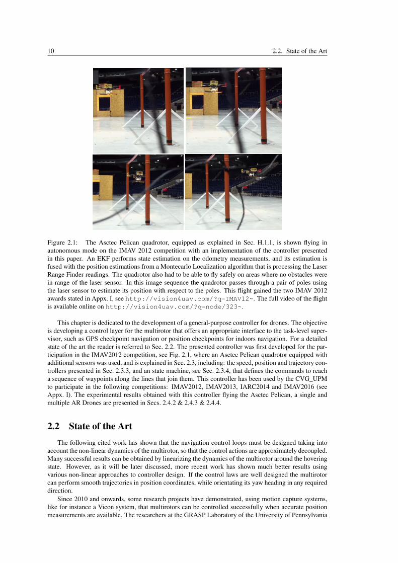
Figure 2.1: The Asctec Pelican quadrotor, equipped as explained in Sec. H.1.1, is shown flying inautonomous mode on the IMAV 2012 competition with an implementation of the controller presentedin this paper. An EKF performs state estimation on the odometry measurements, and its estimation isfused with the position estimations from a Montecarlo Localization algorithm that is processing the LaserRange Finder readings. The quadrotor also had to be able to fly safely on areas where no obstacles werein range of the laser sensor. In this image sequence the quadrotor passes through a pair of poles usingthe laser sensor to estimate its position with respect to the poles. This flight gained the two IMAV 2012awards stated in Appx. I, see http://vision4uav.com/?q=IMAV12~. The full video of the flightis available online on http://vision4uav.com/?q=node/323~.
This chapter is dedicated to the development of a general-purpose controller for drones. The objectiveis developing a control layer for the multirotor that offers an appropriate interface to the task-level super-visor, such as GPS checkpoint navigation or position checkpoints for indoors navigation. For a detailedstate of the art the reader is referred to Sec. 2.2. The presented controller was first developed for the par-ticipation in the IMAV2012 competition, see Fig. 2.1, where an Asctec Pelican quadrotor equipped withadditional sensors was used, and is explained in Sec. 2.3, including: the speed, position and trajectory con-trollers presented in Sec. 2.3.3, and an state machine, see Sec. 2.3.4, that defines the commands to reacha sequence of waypoints along the lines that join them. This controller has been used by the CVG_UPMto participate in the following competitions: IMAV2012, IMAV2013, IARC2014 and IMAV2016 (seeAppx. I). The experimental results obtained with this controller flying the Asctec Pelican, a single andmultiple AR Drones are presented in Secs. 2.4.2 & 2.4.3 & 2.4.4.
2.2 State of the ArtThe following cited work has shown that the navigation control loops must be designed taking into
account the non-linear dynamics of the multirotor, so that the control actions are approximately decoupled.Many successful results can be obtained by linearizing the dynamics of the multirotor around the hoveringstate. However, as it will be later discussed, more recent work has shown much better results usingvarious non-linear approaches to controller design. If the control laws are well designed the multirotorcan perform smooth trajectories in position coordinates, while orientating its yaw heading in any requireddirection.
Since 2010 and onwards, some research projects have demonstrated, using motion capture systems,like for instance a Vicon system, that multirotors can be controlled successfully when accurate positionmeasurements are available. The researchers at the GRASP Laboratory of the University of Pennsylvania

Chapter 2. A General Purpose Configurable Controller for Multirotor MAVs 11
have been able to execute very precise trajectory following, using cascade control laws with non-linear de-coupling functions and precise feedforward command laws (Mellinger et al., 2010; B. Y. N. Michael et al.,2010). They have also demonstrated excellent performance in aggressive maneuvering with small AsctecHummingbird quadrotors, such as multi-flips, perching in vertical landing platforms and precise maneu-vers synchronized with environment events. Several experimental tests have been carried out involving4+ quadrotors in collaborative tasks, examples of such experiments are quadrotor swarming 1 (Kushleyevet al., 2012), a swarming artistic quadrotor show 2 , with lighting effects and movement, that took placeon Cannes Lions Festival of Creativity 2012; and the construction of small-sized buildings using toyconstruction sets 3.
In a similar research line, also making use of a motion capture system, the ETH - IDSC - FlyingMachine Arena project at the Eidgenössische Technische Hochschule Zürich (ETHZ), have also demon-strated impressive quadrotor flight performance on aggressive maneuvering (S. et al., 2010), and synchro-nizing with music (Schölling et al., 2010). The synchronization with music has been shown playing thepiano4 and performing diverse navigation maneuvers following the rhythm of music5. The multirotorplatforms used in this lab are Asctec Hummingbird quadrotors. The synchronization between multiplesUAS platforms is useful for swarming and the exploration of indoors buildings, so that quadrotors canfly together precisely maneuvering without crashing with each other. The environmental music is used tocreate human emotional appeal to the experiments.
The main issue with these works is the requirement of a structured environment, where a motioncapture system has to be in place. Their research work has been extremely fruitful demonstrating whatmany different control approaches can attain. In principle these controllers should perform equally welloutside these environments, if they are fed with a good enough state estimate. However, it is importantto know what is possible for a quadrotor to do outside such structured environments. By that time, therewere research groups that had shown already good autonomous multirotor navigation capabilities usingonly GPS positioning data, or performing (SLAM) during building exploration.
The STARMAC project 6, from the Stanford University shows competitive outdoors performance intrajectory tracking (Hoffmann, Gabriel M et al., 2008) relying only on GPS. Unlike both prior researchlabs, the STARMAC (, 2012) is a bigger multirotor, about 80x80 cm large; and it is also designed by theStanford and Berkeley Universities. Prior work for post-disaster assessment was presented on (Hoffmann,Waslander, et al., 2006). Their work has also been focused on the study of the aerodynamic disturbancesthat are present during quadrotor navigation, for example in the stall turn maneuver (Hoffmann, G.M. etal., 2009), where the multirotor has to change its navigation direction to move backwards. An interestingstudy, from both the theoretical and experimental point of view, was done in the work (Gillula et al., 2010),where the STARMAC platform was able to make single-flip maneuvers in an outdoors environment 7. Thecalculations performed in this study, would allow a quadrotor to determine if a maneuver can be performedsuccessfully, and how near would it be to instability. The control laws used in the STARMAC projectsremained relying on cascade control laws around the hovering linearized state and that took into accountthe non-linear decoupling, using the yaw, of the pitch and roll commands.
Around that time other impressive work, not involving the usage of tracking systems, had been per-formed. The project on collaborative and swarming of multirotor platforms, like the Collaborative Micro-drones project (Quaritsch et al., 2008), works at the GRASP Lab (N. Michael et al., 2012) and the sFlyproject 8 (Scaramuzza et al., 2013). In terms of control, one of the biggest contributions of the sFly projectwas to show that their visual-inertial based architecture could function quite well even with a gap of 1 sec-ond between image measurements (Weiss et al., 2012), which were simulated as pose measurements. Thispaper really showed what a well integrated IMU sensor can attain, in terms of adding robustness to thewhole architecture. In terms of autonomous exploration using quadrotors, some works also have shownthat it was possible for a quadrotor to explore a man-made environments using different sensors: likedLIDAR (A. G. Bachrach, 2009; Shen, N. Michael, et al., 2011), LIDAR and Stereo Cameras (Achteliket al., 2009; A. Bachrach et al., 2011), Stereo cameras only (Heng et al., 2014) and Kinect sensors (A. S.
1https://www.youtube.com/watch?v=YQIMGV5vtd4 , 20122http://www.uasvision.com/2012/07/06/a-flying-quadrotor-light-show-spectacular/ , 20123http://www.youtube.com/watch?v=W18Z3UnnS_0 , 20114http://www.youtube.com/watch?v=ToACDIXTzo0 , 20105http://www.youtube.com/watch?v=7r281vgfotg , 20116http://www.youtube.com/watch?v=rJ9r2orcaYo , 20087http://www.youtube.com/watch?v=iD3QgGpzzIM , 20098http://www.sfly.org/
12 2.3. Controller Algorithm
Huang et al., 2011). Other groups have increased the situational awareness of the mUAVs using opticalflow sensors and cooperative robots. For instance, a ground vehicle can estimate the position and attitudeof the mUAV (Rudol et al., 2008). These two research works (Lippiello et al., 2011; Zingg et al., 2010)are focused on navigation in corridors and obstacle collision avoidance strategies using multiple opticalflow sensors. In outdoors navigation, optical flow sensors were used in a fixed-wing mUAV in (Zuffereyet al., 2010) to avoid the collision with trees and other obstacles in a GPS waypoint trajectory.
Currently, among the most aggressive maneuvering multirotor research projects performed in unstruc-tured environments are probably the following. Fast dynamic trajectory maneuvering has been achieved inindoors flight using LIDAR and IMU integration, but for a previously mapped environment, by Richter etal. (Richter, Charles et al., 2013). And using a mixture of monocular and stereo vision, Shen et al. (Shen,Shaojie et al., 2013; Shen, Mulgaonkar, et al., 2013) have achieved similar capabilities in both indoorsand outdoors environments with a limited short-time visual mapping capability. However this last UASwas still not able to track trajectories as fast as in Richter et al.’s approach.
Next the related research work will be summarized in terms of the control laws themselves, whetherthey can be considered as linear control laws or non-linear ones. The discussion is first done with con-trollers that are linear or designed by linearizing the quadrotor dynamics. Most of these works explicitlylinearize the multirotor dynamics around the hovering position, and then develop the control law for thelinearized system. Then the control problem is subdivided into the attitude stabilization problem, whichis then used as the inner control loop of a nested control architecture, and into the position control prob-lem (Bouabdallah, Murrieri, et al., 2005; Hoffmann, H. Huang, et al., 2007; B. Y. N. Michael et al., 2010).Some of these works still take into account part of the nonlinear characteristics of the system to improvethe general performances of the controller due to varying thrust requirements when tilted and to the rotordrag (Hoffmann, G.M. et al., 2009); or use different operating modes for trajectory following and hov-ering (Hoffmann, Gabriel M et al., 2008; Mellinger et al., 2010). The performances of quadrotors usingLQR control allows around the hovering positions are well studied in the following articles (Cowlinget al., 2010; Nice, 2004; Valenti et al., 2006). However, as shown in (Castillo, Lozano, et al., 2005) thestability may be lost when the flight develops far from the linearized hovering state. This same work alsoshows how a non-linear controller may keep the stability in these cases.
Now, turning the discussion into research on non-linear controllers. Some of them still rely on thelinearized model around the hovering state (Castillo, Lozano, et al., 2005), and saturating or limiting thevalues of interim control commands, effectively saturating the commanded attitude values (Guenard et al.,2005). Very promising results were shown in the following work that applied backstepping (Bouabdallahand Siegwart, 2005; Madani et al., 2007), sliding mode control techniques to multirotors (Bouabdallahand Siegwart, 2005; D. Lee et al., 2009), and research that separate the attitude control problem from thetranslation one (Kendoul et al., 2010; Raffo et al., 2010), feedback linearization control (Driessen et al.,2004; Fritsch et al., 2012; D. Lee et al., 2009; Mistler et al., 2001) and other techniques (Castillo, Dzul,et al., 2004; Guenard et al., 2005; Hua et al., 2009).
A very influencing work by Taeyoung Lee et al. (T. Lee et al., 2010) was done based on the GeometricControl Theory (Agrachev et al., 2004; Jurdjevic, 1997). Although this work only tested the developedcontrol laws in simulation, it demonstrated the stability qualities of the proposed controller, of exponentialattractiveness for attitude errors of up to 90°, and almost exponential attractiveness for errors of up to 180°;and also was formulated in a way that there were no singularities in terms of the attitude representation.
Another influencing work by Oliver Fritsch et al. (Fritsch et al., 2012) performed quasi-static feedbacklinearization for the translation dynamics using a quaternion formulation for the attitude of the multirotor.First the altitude control loop and the heading are controlled using feedback linearization and then in asecond step the lateral translation is also feedback linearized. This control law can be considered to bebuilt on the differential flatness property of the dynamics of the multirotor.
2.3 Controller Algorithm
In this chapter a navigation controller that uses a set of configurable parameters to be adaptable todifferent quadrotors and sensing options is proposed. It is inspired on previous work from other re-search centers (Hoffmann, Gabriel M et al., 2008; B. Y. N. Michael et al., 2010) and by the STARMACproject (Hoffmann, Waslander, et al., 2006). The proposed controller consists of a main control architec-ture and a state machine that provides trajectory following commands to the main control architecture.

Chapter 2. A General Purpose Configurable Controller for Multirotor MAVs 13
Both subsystems are designed to provide control commands that are consistent with a configurable maxi-mum speed parameter.
First, the overall control architecture is introduced in Sec. 2.3.1. Then a simple multirotor point masskinematic model is described in Sec. 2.3.2. Then the main control architecture, named the middle-levelcontroller, is introduced in Sec. 2.3.3. Then the high level controller state-machine is introduced with thedescription of the configurable parameters that are derived from the modelin Secs. 2.3.4 & 2.3.5 & 2.3.6.Then final part of the chapter introduces the experimental results in Sec.2.4 and the conclusions in Sec. 2.6.
2.3.1 Control Architecture
The goal for the controller design task is to make the multirotor follow a path specified by a sequenceof checkpoints. The general controller architecture, shown in Fig. 2.2, consists of: a mid-level controller,that calculates the actual commands that will be sent to the quadrotor; and a high-level controller thattracks the quadrotor position relative to the desired path and calculates the speed and position referencesfor the mid-level controller. The state estimator that was utilized in the experiments and its related modelare explained in Appx. E & D respectively.
ExtendedKalman Filter
High-Level Controller
Finite-State Machine
speedcommands
positioncommands
yawc
zcstate
estimation
Telemetry
Optical flow
Altitude sensors
IMU
Laser Rane Finder
Distance measurements
Various camerasDown-facing image
Frontal-facing image
Mid
-Lev
el C
on
tro
ller
Quadrotor on CVG Framework
Figure 2.2: General architecture of the controller. The measurements are processed by an estimatorthat includes an EKF and a Particle Filter, which are discussed in Appx. E. Then, in order to minimizethe route time, the controller includes a speed planner in a state machine that sends optimized reachablespeed commands to the mid-level controller. The state estimation is used by the high-level controller todetermine optimized reachable speed commands to the mid-level controller, which sends commands tothe drone through the CVG Framework (Mellado Bataller, I., 2012; Mellado-Bataller, Mejias, et al., 2012;Mellado-Bataller, Pestana, et al., 2013) or its pseudo-equivalent ROS node.
The multirotor is stabilized using odometry-based position estimates and for that reason the boundarieswhere the quality of these estimates is lost must be determined. For instance, the optical flow algorithmthat is calculated on the down-facing images is affected by the texture and reflectiveness of the floor sur-face, the size of the floor texture details, the lighting conditions of the environment and the computingpower of the on-board computer. This characteristics set a maximum speed boundary on the speed esti-mation over which the estimates do not provide meaningful information and may cause the malfunctionof the estimation and control architecture.
For instance, the maximum speed that could be reliably estimated at low altitude by our optical flowalgorithm in the indoors playground where most of the tests where carried out was about 0.5-0.75 m/s,and so, this boundary was used in our indoors tests. Based on our experience, the AR Drone at the samealtitude provides speed estimation feedback even navigating at high speeds, up to 3 m/s. The direction ofthe speed estimation maintains a good accuracy at all working conditions if the yaw rotations are kept low.On the other hand, the absolute value of the speed can be affected by several conditions. For example,when the drone switches from ultrasound sensor based to pressure-only based altitude estimation, theaccuracy of the speed estimates is degraded. Also the speed measurement at speed in the 2-3 m/s speedrange is not accurate, but its enough to keep our controller architecture working.

14 2.3. Controller Algorithm
2.3.2 Multirotor Point Mass Kinematic Model
A multirotor is a flying vehicle that propels itself by pointing the thrust force in the required directionand thus can be simplified as a point mass moving in the 3D space. The thrust force is perpendicular thepropeller’s rotating surface, as shown in Fig. 2.3] The vehicle tilts to exert force in the horizontal plane,and changes the average propeller speeds to control the amount of thrust force. A maximum speed is setin practice by various reasons, for instance, due to the aerodynamic friction of the movement through theair. It is also important to take into account that the multirotor is commanded using feedback loop controllaws that produce a response that can be characterized by a set of parameters. The speed planner can takeadvantage of a simple kinematic model built upon these facts in order to take decisions.
The body frame, {Xm, Ym, Zm}, of the vehicle, shown in Fig. 2.3, is described as follows. The{Xm, Ym} axis are horizontal and the Zm axis points down to the floor. The Xm axis points to the frontof the vehicle and the Ym axis points to the right obtaining a orthonormal right-handed reference frame.The euler angles are denoted {φ , roll}, {θ ,pitch} and {ψ,yaw}, and they define the rotation of the thebody frame, {Xm, Ym, Zm}, with respect to the world frame, {X , Y, Z}.
φψ
θ
T2
T4
T1T3 M2
M3M1
M4
Figure 2.3: Free body diagram of a quadrotor. The four propellers, and each of their performed thrust Tiand torque Mi are labeled 1-4. The euler angles are denoted {φ , roll}, {θ ,pitch} and {ψ,yaw}
The quadrotor rigid body dynamics model, see Eq. 2.1 and Fig. 2.3, is infered from physical laws asexplained in Appx. D:
Ixφ = ψ θ (Iy− Iz)+ l (T1 +T2−T3−T4)
Iyθ = φ ψ (Iz− Ix)+ l (T1 +T4−T2−T3)
Izψ = θ φ (Ix− Iy)+∑4i=1Mi (2.1)
mx = (−sinφ sinψ− cosφ sinθ cosψ)∑4i=1Ti−K f r x2
my = (−cosφ sinθ sinψ + sinφ cosψ)∑4i=1Ti−K f r y2
mz = mg− cosθ cosφ ∑4i=1Ti−K f r z2
Where the following variables have been introduced: the position of the quadrotor with respect to theworld frame is denoted by the {x, y, z} coordinates, the attitude of the vehicle is represented by the yawψ , pitch θ and roll φ euler angles; the quadrotor rigid body is characterized by its mass m and its threeprincipal mass moments of inertia {Ix, Iy, Iz}, each propeller i generates a thrust Ti and a heading torqueMi, K f r is an aerodynamic friction constant and the l constant is the arm between each pair of thrusts, inthis case the distance between the propellers 1 and 2, as denoted in Fig. 2.3.
The following control loops are usually implemented inside the autopilot board of the multirotor: theattitude (roll, φ , pitch, θ , and yaw, ψ) control loops and altitude, z, control loop. The autopilot boardsusually accept roll, pitch, yaw speed and altitude speed references. So that the saturation bounds for thesevariables is set by the autopilot board and drone capabilities. Thus, it is only required to further developthe equations of movement in the horizontal plane.
If the flight is performed at constant altitude then, ∑4i=1 Ti ≈ mg, and taking the approximation to low
roll and pitch angles, then the equations that define the mouvement in the horizontal plane are derived
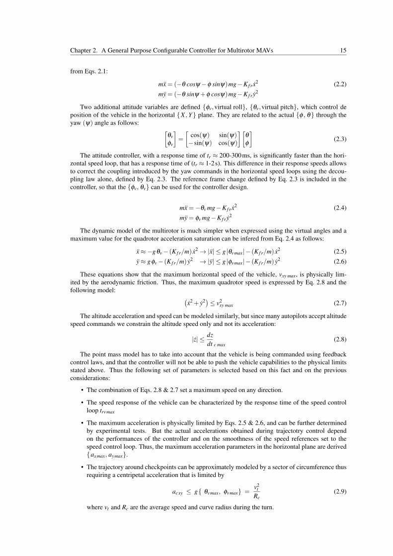
Chapter 2. A General Purpose Configurable Controller for Multirotor MAVs 15
from Eqs. 2.1:
mx = (−θ cosψ−φ sinψ)mg−K f r x2 (2.2)
my = (−θ sinψ +φ cosψ)mg−K f r y2
Two additional attitude variables are defined {φv,virtual roll}, {θv,virtual pitch}, which control deposition of the vehicle in the horizontal {X , Y} plane. They are related to the actual {φ , θ} through theyaw (ψ) angle as follows: [
θvφv
]=
[cos(ψ) sin(ψ)−sin(ψ) cos(ψ)
][θ
φ
](2.3)
The attitude controller, with a response time of tr ≈ 200-300ms, is significantly faster than the hori-zontal speed loop, that has a response time of (tr ≈ 1-2s). This difference in their response speeds allowsto correct the coupling introduced by the yaw commands in the horizontal speed loops using the decou-pling law alone, defined by Eq. 2.3. The reference frame change defined by Eq. 2.3 is included in thecontroller, so that the {φv, θv} can be used for the controller design.
mx =−θv mg−K f r x2 (2.4)
my = φv mg−K f r y2
The dynamic model of the multirotor is much simpler when expressed using the virtual angles and amaximum value for the quadrotor acceleration saturation can be infered from Eq. 2.4 as follows:
x≈−gθv− (K f r/m) x2→ |x| ≤ g |θvmax|− (K f r/m) x2 (2.5)
y≈ gφv− (K f r/m) y2 → |y| ≤ g |φvmax|− (K f r/m) y2 (2.6)
These equations show that the maximum horizontal speed of the vehicle, vxy max, is physically lim-ited by the aerodynamic friction. Thus, the maximum quadrotor speed is expressed by Eq. 2.8 and thefollowing model: (
x2 + y2)≤ v2xy max (2.7)
The altitude acceleration and speed can be modeled similarly, but since many autopilots accept altitudespeed commands we constrain the altitude speed only and not its acceleration:
|z| ≤ dzdt c max
(2.8)
The point mass model has to take into account that the vehicle is being commanded using feedbackcontrol laws, and that the controller will not be able to push the vehicle capabilities to the physical limitsstated above. Thus the following set of parameters is selected based on this fact and on the previousconsiderations:
• The combination of Eqs. 2.8 & 2.7 set a maximum speed on any direction.
• The speed response of the vehicle can be characterized by the response time of the speed controlloop trvmax
• The maximum acceleration is physically limited by Eqs. 2.5 & 2.6, and can be further determinedby experimental tests. But the actual accelerations obtained during trajectotry control dependon the performances of the controller and on the smoothness of the speed references set to thespeed control loop. Thus, the maximum acceleration parameters in the horizontal plane are derived{axmax, aymax}.
• The trajectory around checkpoints can be approximately modeled by a sector of circumference thusrequiring a centripetal acceleration that is limited by
acxy ≤ g{ θvmax, φvmax} =v2
t
Rc(2.9)
where vt and Rc are the average speed and curve radius during the turn.
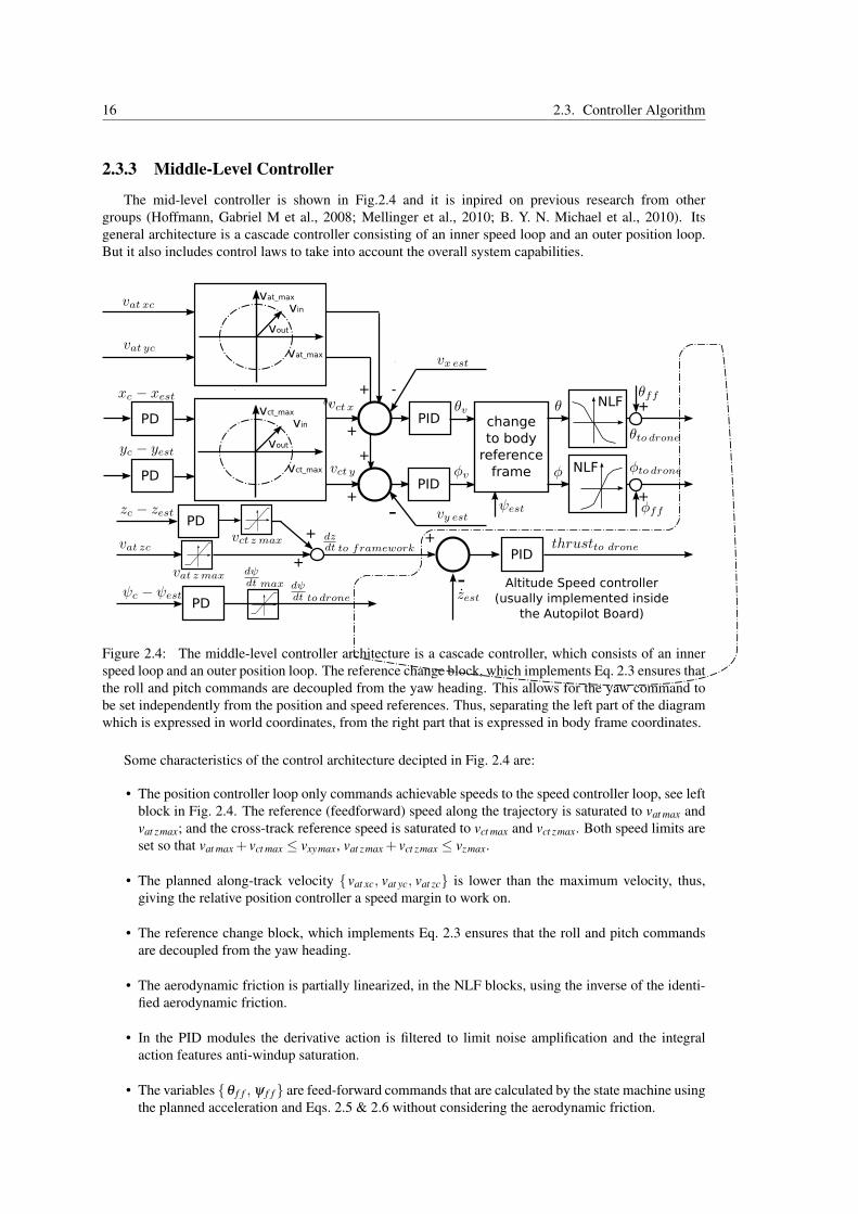
16 2.3. Controller Algorithm
2.3.3 Middle-Level Controller
The mid-level controller is shown in Fig.2.4 and it is inpired on previous research from othergroups (Hoffmann, Gabriel M et al., 2008; Mellinger et al., 2010; B. Y. N. Michael et al., 2010). Itsgeneral architecture is a cascade controller consisting of an inner speed loop and an outer position loop.But it also includes control laws to take into account the overall system capabilities.
vct_max
vct_max
+
+PID
-
+
+
-
NLF
PIDNLF
changeto body
referenceframe
PD
PD
+
-PID
PD
PD
vat_max
vat_max
vin
vout
vin
vout
+
+
+
+
Altitude Speed controller(usually implemented inside
the Autopilot Board)
Figure 2.4: The middle-level controller architecture is a cascade controller, which consists of an innerspeed loop and an outer position loop. The reference change block, which implements Eq. 2.3 ensures thatthe roll and pitch commands are decoupled from the yaw heading. This allows for the yaw command tobe set independently from the position and speed references. Thus, separating the left part of the diagramwhich is expressed in world coordinates, from the right part that is expressed in body frame coordinates.
Some characteristics of the control architecture decipted in Fig. 2.4 are:
• The position controller loop only commands achievable speeds to the speed controller loop, see leftblock in Fig. 2.4. The reference (feedforward) speed along the trajectory is saturated to vat max andvat zmax; and the cross-track reference speed is saturated to vct max and vct zmax. Both speed limits areset so that vat max + vct max ≤ vxymax, vat zmax + vct zmax ≤ vzmax.
• The planned along-track velocity {vat xc, vat yc, vat zc} is lower than the maximum velocity, thus,giving the relative position controller a speed margin to work on.
• The reference change block, which implements Eq. 2.3 ensures that the roll and pitch commandsare decoupled from the yaw heading.
• The aerodynamic friction is partially linearized, in the NLF blocks, using the inverse of the identi-fied aerodynamic friction.
• In the PID modules the derivative action is filtered to limit noise amplification and the integralaction features anti-windup saturation.
• The variables {θ f f , ψ f f } are feed-forward commands that are calculated by the state machine usingthe planned acceleration and Eqs. 2.5 & 2.6 without considering the aerodynamic friction.

Chapter 2. A General Purpose Configurable Controller for Multirotor MAVs 17
2.3.4 High-Level Controller - State-MachineThe HL controller is implemented using a Finite State Machine (FSM), Fig. 2.5, which uses the
state estimation from the EKF to calculate the mid-level controller references. The FSM has three statescorresponding to three control strategies: hover in a desired position, follow a straight segment of thetrajectory and turn to head to the next trajectory segment.
Straight Segment navigationat entry: speed planification
calculate mid-controller references
Turn navigation Hoverto Checkpointcalculate
mid-controllerreferences
calculatemid-controller
references
1StraightSegmentEnd
not(LastCheckpoint)LastCheckpoint
not(LastCheckpoint)2 2
TurnEnd1
CheckpointReached CheckpointReachedand
not(CheckpointReached)
Waypoint trajectory following
Hover todesired position
Navigateat reference
speed
Figure 2.5: High-level control finite state machine. The state machine accepts three flying modes:‘waypoint trajectory following’, ‘hover to reference position’ and ’navigate at reference speed’. Thestates correspond to navigation control strategies. The state transitions are activated depending on theposition of the drone relative to the current trajectory.
The main purpose of the FSM is to navigate along a waypoint trajectory, and therefore its main actions,during trajectory tracking, can be summarized as the repetition of the following steps:
1. Follow a straight segment, accelerating at first, and slowing down before reaching the next turn,
2. Around the mid-waypoints of the trajectory, perform a turn controlling the speed direction toachieve a soft alignment with the next straight segment.
The FSM has also two additional operation modes where the quadrotor is controlled either only in positioncontrol, or in speed control. These can be used by the task scheduler to perform certain tasks. Duringtrajectory tracking, every time the controller output is calculated the FSM calculates the planned speed atthe current position vplan(s), where s is a coordinate along the trajectory:
1. The speed, {Vturn i}, inner turn angle, {αi}, and radius, {Rturn i}, at checkpoint i during each turn areprecalculated each time the reference trajectory is changed, for instance when a waypoint is added.The radius is calculated so that the trajectory passes at a distance Rcon f /2 from the checkpoint,where Rcon f is the maximum distance at which the checkpoint is considered to be reached. Theplanned speed for each turn is selected either according to Eq. 2.9 either considering that the turnrequires a stall-turn or turn-around maneuver, vstall turn, which corresponds to a planned speed nearzero.
2. The algorithm explained in Sec. 2.3.5 is used to calculate the planned speed, vplan(s), at the currentposition.
The middle-level (ML) controller, see Fig. 2.2, receives position, {xc, yc, zc}, yaw heading, ψc, speed,{vat xc, vat yc, vat zc}, and tilt feed-forward, {θ f f , ψ f f }, commands from the FSM, as shown in Fig. 2.4.The presented controller allows to use a single mid-level architecture for the three control modes: trajec-tory, position and speed modes. These references to the ML controller are calculated by the FSM in sucha way that the relative position and speed commands are orthogonal:
• The position references [xc, yc, zc] are caltulated projecting the estimated position [ xest , yest , zest ]onto the reference trajectory.
• The along-track speed commands, [vat xc, vat yc, vat zc], are parallel to the trajectory vplan(s)~utangent .
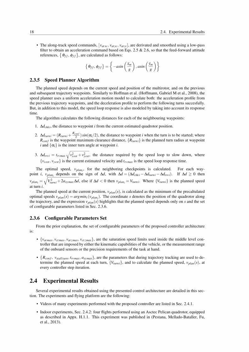
18 2.4. Experimental Results
• The along-track speed commands, [vat xc, vat yc, vat zc], are derivated and smoothed using a low-passfilter to obtain an acceleration command based on Eqs. 2.5 & 2.6, so that the feed-forward attitudereferences,
{θ f f , φ f f
}, are calculated as follows:
{θ f f , φ f f
}=
{−asin
(xm
g
), asin
(ym
g
)}
2.3.5 Speed Planner AlgorithmThe planned speed depends on the current speed and position of the multirotor, and on the previous
and subsequent trajectory waypoints. Similarly to Hoffman et al. (Hoffmann, Gabriel M et al., 2008), thespeed planner uses a uniform acceleration motion model to calculate both: the acceleration profile fromthe previous trajectory waypoints, and the deceleration profile to perform the following turns succesfully.But, in addition to this model, the speed loop response is also modeled by taking into account its responsetime.
The algorithm calculates the following distances for each of the neighbouring waypoints:
1. ∆dchk i, the distance to waypoint i from the current estimated quadrotor position.
2. ∆dturn i = (Rturn i +Rcon f
2 )sin(αi/2), the distance to waypoint i when the turn is to be started; whereRcon f is the waypoint maximum clearance distance, {Rturn i} is the planned turn radius at waypointi and {αi} is the inner turn angle at waypoint i.
3. ∆dtrv i = trvmax
√v2
xest + v2yest , the distance required by the speed loop to slow down, where
{vxest , vyest} is the current estimated velocity and trvmax is the speed loop response time.
The optimal speed, vplani , for the neighboring checkpoints is calculated. For each way-point i, vplani depends on the sign of ∆d, with ∆d = (∆dchk i−∆dturn i−∆dtrv i). If ∆d ≥ 0 then
vplani =√
V 2turn i +2axymax ∆d, else if ∆d < 0 then vplani =Vturn i. Where {Vturn i} is the planned speed
at turn i.The planned speed at the current position, vplan(s), is calculated as the minimum of the precaltulated
optimal speeds vplan(s) = argmini (vplani). The coordinate s denotes the position of the quadrotor alongthe trajectory, and the expression vplan(s) highlights that the planned speed depends only on s and the setof configurable parameters listed in Sec. 2.3.6.
2.3.6 Configurable Parameters SetFrom the prior explanation, the set of configurable parameters of the proposed controller architecture
is:
• {vat max, vct max, vat zmax, vct zmax}, are the saturation speed limits used inside the middle level con-troller that are imposed by either the kinematic capabilities of the vehicle, or the measurement rangeof the onboard sensors or the precision requirements of the task at hand.
• {Rcon f , vstall turn, trvmax, axymax}, are the parameters that during trajectory tracking are used to de-termine the planned speed at each turn, {Vturn i}, and to calculate the planned speed, vplan(s), atevery controller step iteration.
2.4 Experimental ResultsSeveral experimental results obtained using the presented control architecture are detailed in this sec-
tion. The experiments and flying platform are the following:
• Videos of many experiments performed with the proposed controller are listed in Sec. 2.4.1.
• Indoor experiments, Sec. 2.4.2: four flights performed using an Asctec Pelican quadrotor, equippedas described in Appx. H.1.1. This experiment was published in (Pestana, Mellado-Bataller, Fu,et al., 2013).

Chapter 2. A General Purpose Configurable Controller for Multirotor MAVs 19
• Outdoor experiments, Sec. 2.4.3: three flights performed using an AR Drone 2.0 quadrotor, de-scribed in Appx. H.2. This experiment was published in (Pestana, Mellado-Bataller, Sanchez-Lopez, et al., 2014).
• Indoor experiments in a replica of the IMAV 2013 competition environment, Sec. 2.4.4: one flightwith three AR Drone 2.0 quadrotors flying simultaneously in the same area. This experiment waspublished in (Pestana, Sanchez-Lopez, et al., 2015).
2.4.1 Videos of ExperimentsSeveral playlists are uploaded in YouTube related to experiments and flights by the CVAR/CVG
(UPM) that have been performed using the proposed controller. The main ones are related to the par-ticipation of our research group in international MAV competitions, for details on this events with theircorresponding achieved results the reader is refered to Appx. I.. Therefore the following list is given:
• International Micro Air Vehicle Conference and Flight Competition 2016 (IMAV 2016),video playlist: https://goo.gl/tdZyGu.
• Asia Venue of the AUVSI International Aerial Robotics Competition 2014 (IARC 2014),video playlist: https://goo.gl/bEvK3F.
• International Micro Air Vehicle Conference and Flight Competition 2013 (IMAV 2013),video playlist: https://goo.gl/KosWKH.
• International Micro Air Vehicle Conference and Flight Competition 2012, (IMAV 2012),video playlist: https://goo.gl/PRns2D.
2.4.2 Experimental Results - Indoors FlightThis section describes four separate experimental flights that show the navigation capabilities of
the presented controller architecture. These flights were performed using an Asctec Pelican quadrotor,equipped as described in Sec. H.1.1. These flights were originally performed as part of the publica-tion (Pestana, Mellado-Bataller, Fu, et al., 2013). All the flights are trajectory tracking tests in autonomousnavigation carried out in an indoor espacious room, simulating a GPS-denied situation. Thus, the GPS sig-nal is not used in the estimation algorithms. One of the tests consists on the Pelican following a trajectoryin a vertical XZ plane, see Fig. 2.6. There is a second test performed by this quadrotor following a squarehorizontal trajectory shown on Fig. 2.7. The last two tests were done using the AR Drone following thehorizontal eight-shaped trajectory shown in Figs. 2.8 & 2.9. A summary of the controller performancesin these tests is shown in Table 2.1.
The Pelican was configured with the following parameters values. {vat max, vct max , vat zmax, vct zmax}where fixed to 0.5 m/s. and the horizontal speed was constrained with an additional saturation to0.70 m/s. This limitation ensured that the speed reference for the speed control loop was inside the reli-able measurement range of our optical flow implementation. The FSM parameters were: Rcon f = 0.30 m,vstall turn = 0.30 m/s, trvmax was set to 0 s because the planned speed was always lower than 0.7 m/s (thisparameter does not give an advantage in this situation), and the maximum acceleration axymax was set to0.5 m/s2.
The vertical flight of the Pelican on the XZ plane shown in Fig. 2.6 consisted on two laps. The meanand maximum tracking errors during the test were 0.15 m and 0.38 m correspondingly. The vehiclenavigated at a mean and maximum speeds of 0.42 m/s and 0.7 m/s. During half of the flight the vehiclewas commanded to change its yaw heading, without affecting the trajectory tracking objectives.
The horizontal flight of the Pelican shown in Fig. 2.7 was carried out setting a constant yaw headingreference so that the results could be compared with those of the previous test, shown on Fig. 2.6. Themean and maximum tracking errors during the test were 0.09 m and 0.27 m correspondingly. The Pelicannavigated at a mean and maximum speeds were 0.51 m/s and 0.60 m/s. The trajectory controller featuressimilar performances on both types of trajectory.

20 2.4. Experimental Results
0
2
4
6
8
−2
0
2
11.5
22.5
X coordinate [m]
Z c
oo
rdin
ate
[m
]
Y coordinate [m]
EKF reference limits
0
2
4
−2
0
2
11.5
22.5
X coordinate [m]
Z c
oord
inate
[m
]
Y coordinate [m]
EKF reference Heading limits
Figure 2.6: Asctec Pelican test on a vertical eight-shape trajectory, where two laps were com-pleted. The graph above shows the trajectory in the XYZ space, and the bounding box graph(‘limits’ on the legend) shows that the Y error was kept low. A video of the test is available onhttp://vision4uav.com/?q=node/338 . During the second lap the yaw reference was changed repeatedlywithout affecting the trajectory tracking.
2
4
−3−2
−10
0
1
2
X coordinate [m]
Z c
oord
inate
[m
]
Y coordinate [m]
EKF reference limits
Figure 2.7: Asctec Pelican test on horizontal square trajectory. The quadrotor performed two turns car-rying out the trajectory tracking task. The altitude hold worked successfully during this test, and the yawheading reference was kept constant.
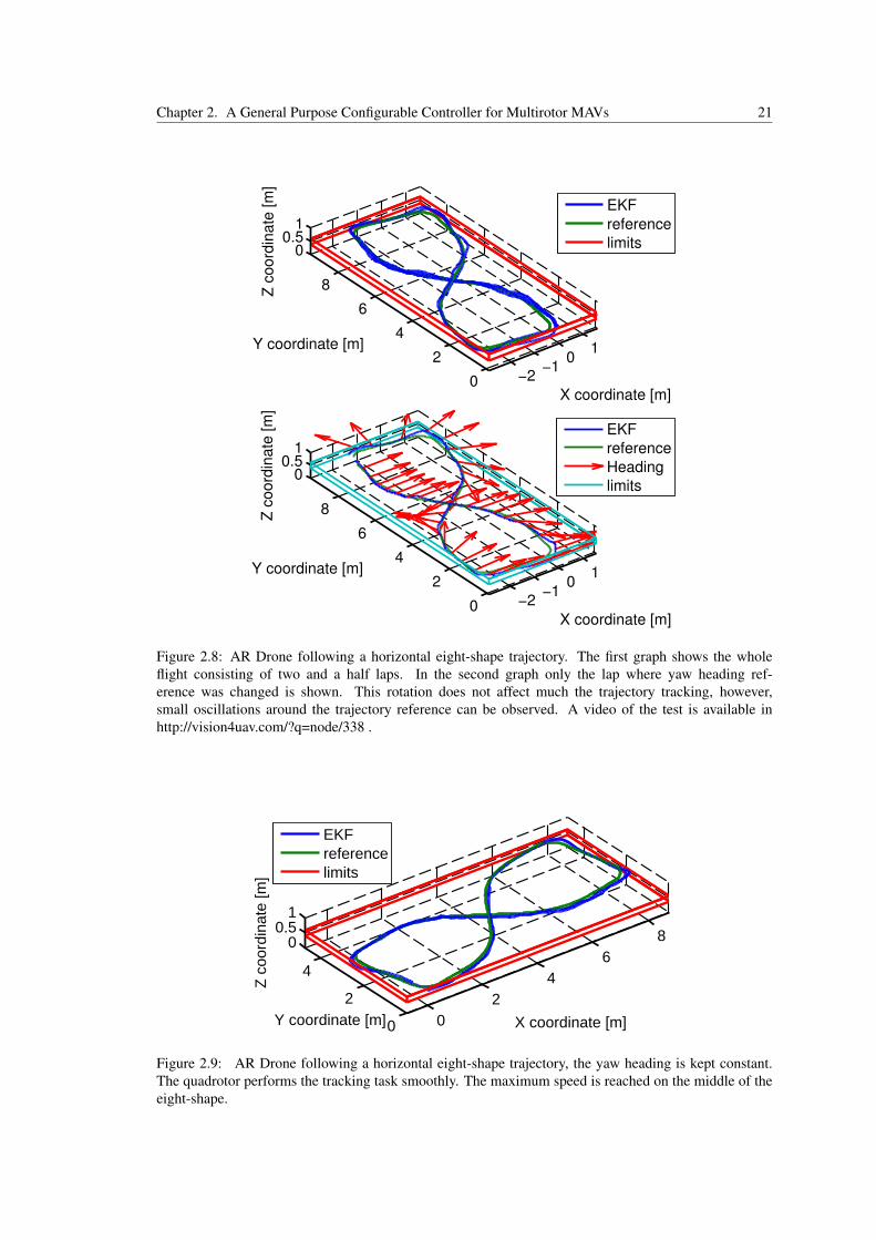
Chapter 2. A General Purpose Configurable Controller for Multirotor MAVs 21
−2−1
01
0
2
4
6
8
00.5
1
X coordinate [m]
Z c
oord
inate
[m
]
Y coordinate [m]
EKF
reference
limits
−2−1
01
0
2
4
6
8
00.5
1
X coordinate [m]
Z c
oord
inate
[m
]
Y coordinate [m]
EKF
reference
Heading
limits
Figure 2.8: AR Drone following a horizontal eight-shape trajectory. The first graph shows the wholeflight consisting of two and a half laps. In the second graph only the lap where yaw heading ref-erence was changed is shown. This rotation does not affect much the trajectory tracking, however,small oscillations around the trajectory reference can be observed. A video of the test is available inhttp://vision4uav.com/?q=node/338 .
0
2
4
6
8
0
2
4
00.5
1
X coordinate [m] Y coordinate [m]
Z c
oord
inate
[m
]
EKF
reference
limits
Figure 2.9: AR Drone following a horizontal eight-shape trajectory, the yaw heading is kept constant.The quadrotor performs the tracking task smoothly. The maximum speed is reached on the middle of theeight-shape.

22 2.4. Experimental Results
The AR Drone was configured with the following parameters values. The maximum horizontalspeed was set to 2 m/s, where vat max = 1.4 m/s, vct max = 0.8 m/s. The FSM parameters were set toRcon f = 0.50 m, vstall turn = 0.25 m/s, trvmax = 1.7 s, and the maximum acceleration to axymax = 0.4 m/s2.The configuration parameters were selected to work on trajectories made up of short segments, with theobjective of optimizing speed while keeping low tracking error.
Fig. (Pel.) 2.6 (Pel.) 2.7 (ARD.) 2.8 (ARD.) 2.9dmean [m] 0.15 0.09 0.10 0.09dmax [m] 0.38 0.27 0.29 0.28
vmean [m/s] 0.42 0.51 0.61 0.61vmax [m/s] 0.70 0.60 1.10 1.10
Table 2.1: Summary of results of the experimental tests: average, dmean, and maximum, dmax, trackingerror; average, vmean, and maximum, vmax, speed during the test
Both flights shown in Figs. 2.8 & 2.9, were performed following the same eight-shape trajectory tocheck whether the trajectory control actions are decoupled from the yaw reference. The obtained resultswere a mean and maximum tracking errors of 0.09 m and 0.28 m correspondingly. The vehicle navigatedat a mean and maximum speeds of 0.61 m/s and 1.10 m/s. The similarity between both tests demonstratesthat the yaw heading is approximately decoupled from the trajectory tracking.
The flights of both quadrotors were mostly unaffected during yaw heading rotation. In the flights ex-posed in this section the yaw rotation speed was about 25-30 ◦/s. The experimental data clarify, however,that both vehicles tend to oscillate around the reference trajectory during the yaw rotation, a comparisonbetween Figs. 2.8 & 2.9 shows this fact. High yaw rotation speeds do affect the position control, but thisis not an interesting action for many applications.
2.4.3 Experimental Results - Outdoors FlightThis section describes three separate experimental flights that show the navigation capabilities of the
presented controller architecture. These flights were performed using an AR Drone 2.0 quadrotor. Allthe flights are trajectory tracking tests in autonomous navigation carried out in an outdoors environment,simulating a GPS-denied situation. Thus, GPS was unavailable and unused during the tests. All the flightswere performed with the AR Drone 2.0 with the outdoors hull. These flights were originally performed aspart of the publication (Pestana, Mellado-Bataller, Sanchez-Lopez, et al., 2014). The flight trajectories areshown in Figs. 2.10 & 2.11 & 2.12. The system has been tested following regular polygon trajectories onthe XY plane, with varying altitude on each waypoint, of values of 0-3 m higher than the first checkpoint’saltitude. A summary of the controller performances in these tests is shown in Table 2.2.
Parameter dmean dmax vmean vmax ∆Lmean ∆ttestunits [m] [m] [m/s] [m/s] [m] [s]
Square, Fig. 2.10 0.17 0.70 0.92 1.90 7.72 123.0Hexagon, Fig. 2.11 0.31 1.71 1.09 1.95 7.75 123.0Octagon, Fig. 2.12 0.32 2.90 1.17 2.10 7.75 95.0
Table 2.2: Summary of results of the experimental tests obtained for the trajectories shown inFigs. 2.10 & 2.11 & 2.12. The specified parameters are: average, dmean, and maximum, dmax, track-ing error; average, vmean, and maximum, vmax, speed along-trajectory; ∆Lmean , mean distance betweenwaypoints and ∆ttest , duration of the test. The tested trajectories and poligons on the XY plane, withvarying values of altitude on each waypoint. The tracking error is calculated from the odometry based po-sition estimates. The mean and maximum speed are calculated taking into account the component alongthe trajectory, where the number of laps on each test was 2−3 laps.
The AR Drone 2.0 was configured with the following parameters values. The maximum horizontalspeed was set to 2.75 m/s, where vat max = 2.0 m/s, vct max = 0.75 m/s. The FSM parameters were set toRcon f = 0.25 m, vstall turn = 0.25 m/s, trvmax = 1.20 s, and the maximum acceleration to axymax = 0.70 m/s2.

Chapter 2. A General Purpose Configurable Controller for Multirotor MAVs 23
The configuration parameters were selected to obtain high speeds on the straight segments, with theobjective of studying the controller performance on this configuration on outdoors environments.
Each experiment is shown in one figure: the first experiment consisted of a pseudo-square trajectoryshown on Fig. 2.10, the second one was a pseudo-hexagon shown on Fig. 2.11, and the last one was apseudo octagon shown on Fig. 2.12. As shown the drone follows a trajectory made out of straight segmentsand circle segments around the corners. The first graphs {(a), (c) and (e)} show only the trajectoryreference and the estimated position, and the second ones {(b), (d) and (f)} show also the yaw headingduring one of the laps. As can be appreciated from the graphs; the yaw control can be handled separatelyfrom the position control.
The trajectory tracking position error is measured against the odometry based position estimation. Asexpected this estimation is not accurate, and accumulates error over time. A ground truth to calculate anaccurate tracking error is difficult to obtain without a motion capture system, which is the reason whyit is not calculated. The drift depends on many circumstances that affect the quality of the optical flowspeed estimation: texture of the floor, size of identifiable features in floor texture, illumination, altitude ofthe flight, yaw rotation speed, etc. To keep a good quality on the position measurements the yaw rotationspeed commands are saturated at 50◦/s, and are usually below 30◦/s. The flights were mostly anaffectedduring yaw heading rotation. In the flights exposed in this section the yaw rotation speed attained valuesof about 30−50◦/s. The experimental data clarify, however, that the vehicle tends to oscillate around thereference trajectory during the yaw rotation. High yaw rotation speeds do affect the position control, but50 ◦/s is an acceptable value for many applications.
The altitude on each experiment was 2.5− 5.5 m, 5.5− 8.5 m and 3.0− 6.0 m respectively. TheAR Drone 2.0 can measure altitude precisely of up to 6 m (Bristeau et al., 2011) using the ultrasoundsensor. For higher altitudes the drone has to switch to using the pressure sensor. In practice, the dronetelemetry will show a good tracking on the altitude coordinate, while on reality the vehicle is correctingthe altitude internally moving upwards or downwards. This was specially appreciable during some of theexperiments, but is not visible on the plots because the sensor reading is misleading.
The selected tests show how our architecture is able to deal with moderate winds and how it takes intoaccount automatically the curve inner angles of the trajectory at each waypoint. The trajectories have avarying number of waypoints to provide a varying inside angle of the trajectory at their waypoints. Sincethey are all regular polygons on the XY plane, then the higher the number of waypoints the bigger theinner angles of the trajectory will be, allowing for faster passes through them. This is appreciated by themean speed during trajectory tracking, see vmean in Table 2.1. The other factor that affects the maximumand mean speeds, vmax and vmean respectively, is the distance between waypoints; but all the trajectorieswhere performed with similar distances. Longer distances between waypoints allow the multirotor toaccelerate to and decelerate from higher speeds.
In some occasions, the drone drifts in the curves of the trajectory. But this behavior is not determinis-tic and the same error is not committed in every corner and is not even repeated on the next lap. However,it could be avoided lowering the axymax and trvmax to more restrictive values. It would also be convenientto have separate values of acceleration for the curves and the straight lines, as the controller architecturedoes not perform equally well on straight trajectory segments than in the curves. Then the solutions areimproving the controller, or adding parameters to the speed planning algorithm to take into account thisissue. Another occasional behavior is that the odometry error may increase substantially and the dronemight perform a 20-50% bigger trajectory than commanded, due to odometry estimation errors; or subse-quently accumulate a constant drift per lap on a certain direction. This behavior might be triggered by theAR Drone’s altitude sensor switching solution, but we do not have experimental evidence to ascertain thesource of this occasional problem.

24 2.4. Experimental Results
−6−4
−20
2
02
46
8
−5−4−3
(a)
x [m]y [m]
z [
m]
position est.
reference
−8−6
−4−2
02
02
46
810
−5−4−3
(b)
x [m]y [m]
z [m
]
position est.
reference
heading
Figure 2.10: Pseudo-square trajectory following experimental test on an outdoors environment performedusing our achitecture and an AR Drone 2.0. The (a) graph shows the referece and followed trajectoryin the XYZ space, and the (b) graph additionally shows the vehicle heading during the second lap ofthe experiment were the yaw controller interaction with the trajectory following task was tested. Thetrajectory is a square on the XY plane with varying values of altitude, on the 2.5-5.5 m range, at eachcheckpoint. The test consisted on three laps, where the yaw heading control was tested on the secondlap, which is plotted on graph (b). Some performance parameters obtained from this test are shown inTable 2.1.

Chapter 2. A General Purpose Configurable Controller for Multirotor MAVs 25
−10
−5
0
0
5
10
−8
−6
(c)
x [m]y [m]
z [m
]position est.
reference
−10
−5
0
0
5
10
−8−7−6
(d)
x [m]y [m]
z [m
]
position est.
reference
heading
Figure 2.11: Pseudo-hexagon trajectory following experimental test on an outdoors environment per-formed using our achitecture and an AR Drone 2.0. The (c) graph shows the referece and followed tra-jectory in the XYZ space, and the (d) graph additionally shows the vehicle heading during the second lapof the experiment were the yaw controller interaction with the trajectory following task was tested. Thetrajectory is an hexagon on the XY plane with varying values of altitude, on the 5.5-8.5 m range, at eachcheckpoint. The test consisted on three laps, where the yaw heading control was tested on the secondlap, which is plotted on graph (d). Some performance parameters obtained from this test are shown inTable 2.1.

26 2.4. Experimental Results
−15−10
−50
0
5
10
15
−6
−4
(e)
x [m]y [m]
z [m
]
position est.
reference
−15−10
−50
0
5
10
15
−6
−4
(f)
x [m]y [m]
z [
m]
position est.
reference
heading
Figure 2.12: Pseudo-octagon trajectory following experimental test on an outdoors environment per-formed using our achitecture and an AR Drone 2.0. The (e) graph shows the referece and followed tra-jectory in the XYZ space, and the (f) graph additionally shows the vehicle heading during the second lapof the experiment were the yaw controller interaction with the trajectory following task was tested. Thetrajectory is an octagon on the XY plane with varying values of altitude, on the 3.0-6.0 m range, at eachcheckpoint. The test consisted on two laps, where the yaw heading control was tested on the second lap,which is plotted on graph (f). The test was interrupted at the end of the second lap due to poor WiFiperformance. Some performance parameters obtained from this test are shown in Table 2.1.

Chapter 2. A General Purpose Configurable Controller for Multirotor MAVs 27
2.4.4 Experimental Results - Flights in IMAV2013 ReplicaIn this section one experimental test with three AR Drone 2.0 quadrotors flying simultaneously is
described. This experiment was published in (Pestana, Sanchez-Lopez, et al., 2015). This test shows theperformance of our architecture in a replica of the IMAV 2013 competition environment.
Waitingto avoidcollision
Performinglaps
Performinglaps
Performinglaps
pole obstacleavoidance
(a) (b)
(c) (d)
Figure 2.13: A navigation architecture has been designed for AR Drone 2.0 platforms. Figure (a) shows apicture of three of these quadrotors. The experiments are performed in a replica of the IMAV 2013 IndoorChallenge environment, shown in figure (b). This environment consists of a wall with two windows andeight poles. The position of the wall is previously known but not the location of the windows along it.The wall and the poles represent obstacles that must be avoided by the drones while flying. Only theposition of the four corner poles is previously known. All the poles and the windows are stamped usingArUco visual markers (Garrido-Jurado et al., 2014), see (b) and (c). Figure (c) shows an experimentalflight at the moment when the quadrotors are crossing the unknown poles area. The unknown poles arerobustly located in previous laps, when the drone performs laps around the known poles, ensuring a goodestimation of their positions. The collision avoidance with other agents is solved at the trajectory planningstep. For instance in (d), a drone has to wait until the path to cross the window is free. The flight shown in(c) is described and analyzed in Sec. 2.4.4.3. Videos of this and other flights are available at the websitehttp://www.vision4uav.com/?q=node/386 .

28 2.4. Experimental Results
Aru
co #
id
Figure 2.14: Relevant coordinate frames of our proposed solution. The figure shows a simplified depictionof the IMAV2013 environment: the initial take-off position is shown in gray; the static obstacles, the walland columns, in green; two drones in green and a marker in red. The world coordinate frame, Fworld , islocated in one of the corners of the wall. The frames of the drones, Fdrone1 and Fdrone2; and the marker,Fmarker, are also shown. Only the position of the windows and the four inner columns are not known.
2.4.4.1 Multi-Agent-Level Mission Coordination
For the realization of a multi-robot flight in the IMAV2013 competition, a trajectory planner wasutilized. Visual markers were positioned in the flying field, so that all obstacles were tagged, and thedrones could periodically locate themselves in global coordinates against them. The position in globalcoordinates was known only for part of the visual markers. The trajectory planner module had a mapof the competition environment which was precise except for the position of the windows and part ofthe obstacles. The map is shown in Fig. 2.14. The trajectory planner also knew the position of all flyingdrones. Therefore this module had the capability to deliver obstacle-free trajectories during the flight. Thedrones performed only navigation related missions. The overall expected behavior of the agents duringmission execution is:
• Each agent follows a sequence of waypoints given by its mission specification. The mission sched-uler executes it sequentially.
• During execution, the trajectory planner will attempt to find trajectories that are collision-free. If itfails, the quadrotor will be controlled to stay in the current position.
• The other drones are considered obstacles only when they are inside a 4 m radius from the agents’position. When other drones are nearby, the expected behavior is the following:
– If other robotic agents enter the current trajectory, the trajectory planner will detect it andit will command the trajectory controller, and thus also the quadrotor, to stay in its currentposition while attempting to find a collision-free path to the current waypoint.
– If another robotic agent is on or enters the current waypoint, then the trajectory planner handlesthe situation in the same manner. The trajectory controller is commanded to stay in the currentposition. A new collision-free path will be calculated when the current waypoint is free again.
One interesting characteristic of this multi-robot system is that there is no central mission supervisor.Rather, the synchronization of the drone navigation mission is achieved by the set of rules and conventionsspecified in the Trajectory Planner and the Trajectory Controller, of which one instance is running on eachagent. Arguably, this intelligence does not allow to solve every possible navigation conflict between therobotic agents. However, if the mission is specified correctly unsolvable conflicts will not occur.
The number of drones that can be flown using our architecture is limited by the WiFi bandwidthrequirements of the AR Drones. Experimental testing has shown us, that by limiting the quality of thevideo stream sent by each drone, it is possible to fly up to 9 drones, which share the three availableindependent WiFi channels in groups of 3. The problem is the requirement of the AR Drone 2.0 forvisual-based navigation of sending the imagery to the ground station. Otherwise, using drones with anon-board computer running an instance of our agent-level architecture would allow for higher numbers ofdrones to fly simultaneously.

Chapter 2. A General Purpose Configurable Controller for Multirotor MAVs 29
2.4.4.2 Mission specification - Flights in IMAV2013 Replica
The mission specification is identical for all drones flying and corresponds to the following sequenceof tasks, see Fig. 2.14:
1. Start the agent flight architecture (autopilot interface, controller, state estimators, visual markerdetector, trajectory planner, mission scheduler and agent monitor) and take-off,
2. Move in front of the window and then move to one corner of the poles area (thus, crossing the bigwindow). During this task, the quadrotor is controlled to look at the poles area perpendicularly tothe wall, which results in a constant yaw reference,
3. Perform laps around the poles area for 3 minutes,
4. Cross the poles area moving towards the upper right corner of the map,
5. Navigate to the final scoring location and perform the landing, hovering and landing task specifiedin the IMAV 2013 rules. During this task, the quadrotor is controlled to look at the poles areaperpendicularly to the wall, which results in a constant yaw reference.
The laps and the crossing through the unknown poles area tasks are specified so that all the drones willprobably navigate in the same direction. This mission specification requirement minimizes the occurrenceof navigation conflicts. During tasks 3 and 4, the quadrotor is controlled to look at a specific cornercolumn. The laps around the poles area are specified by waypoints in the corners and in the middle pointsof the square lap. The drone switches to looking at the next column in these middle points.
Considering the size of the map, 10x15m, and the size of the AR Drones, around 52x52cm, the com-petition environment gets relatively crowded when more than 5 drones are navigating around the columns’area. In our experiments, the main factor, more important than localization and control inaccuracies, thataffects the selected safety distance between quadrotors is the necessity to avoid interference among theultrasound altimeters of the AR Drones. Additionally to the altimeter problems, in real flights, WiFibandwidth limitations may also limit the maximum number of drones to around six, and in our experiencemaximally nine, drones flying simultaneously.
2.4.4.3 Experimental Results - Flights in IMAV2013 Replica
The mission specification was described in Sec. 2.4.4.1. Subfig. 2.13(c) shows the drones attemptingto cross the unknown pole area during this flight. And the figures 2.15 and 2.16 summarize the experi-mental flight. In these figures, the obstacles, the wall with two windows and the eight poles, are shown inblack. The trajectories executed by the drones, as estimated by the localization module, are shown withlines. The agents know the position of the four corner poles and the wall, and the size of the windows; butneed to estimate the position of the four unknown poles and the windows.
A 2D overview plot of the flight is shown in Fig. 2.15. As shown in the videos, the quadrotors arecommanded to look at specific known poles to control the odometry position error. At the middle of eachside the agents are commanded to look at the next corner pole. At this moment the position estimatemight change. These events increase the localization error in specific points of the mission execution andtrigger the planning of new trajectories. In this flight they occur repeatedly in the points [−0.5,7.75] and[5.5,10.5], see Fig. 2.15.
The explained emergent synchronized behavior of the drones is shown in Fig. 2.16. The missionis specified to minimize navigation conflicts and maximize the final achieved competition score. Forexample all the agents perform laps in the same direction.
In Fig. 2.16 the current estimated position and orientation of each quadrotor is shown with a markerand an arrow, the last 30 seconds of the executed trajectory are shown by a line and the currently plannedtrajectory is shown by a segmented line with markers. Subfigs. 2.16(a)-(d) show the startup sequence,where the drones cross the big window and the automatic synchronization is achieved. Subfigs. 2.16(e)-(f) show the final steps of the mission execution, where the drones cross the unknown pole area andland in the final position. More details of the execution of this mission can be read in the caption of theexperiment figures 2.15 and 2.16.
Additionally, Fig. 2.17 shows, for drone1 only, plots of the drift-free (green) and the odometry-based(blue) estimates. The known environment elements are shown in black and the progressively mapped
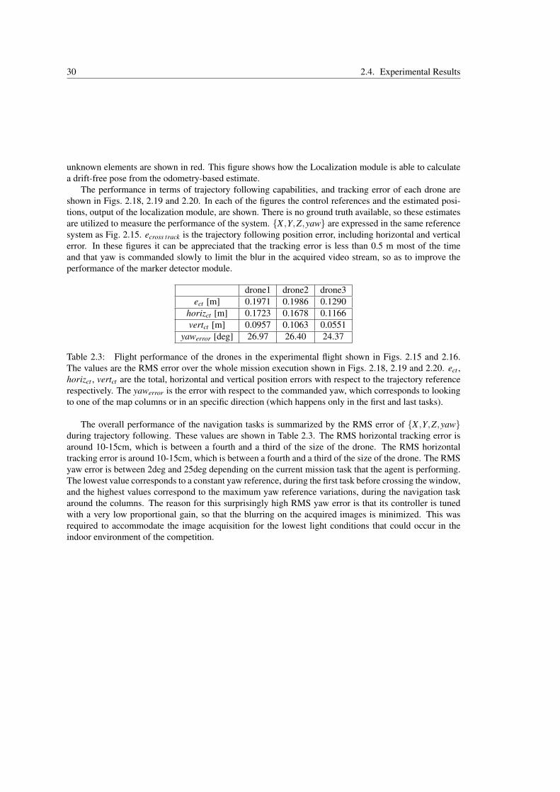
30 2.4. Experimental Results
unknown elements are shown in red. This figure shows how the Localization module is able to calculatea drift-free pose from the odometry-based estimate.
The performance in terms of trajectory following capabilities, and tracking error of each drone areshown in Figs. 2.18, 2.19 and 2.20. In each of the figures the control references and the estimated posi-tions, output of the localization module, are shown. There is no ground truth available, so these estimatesare utilized to measure the performance of the system. {X ,Y,Z,yaw} are expressed in the same referencesystem as Fig. 2.15. ecross track is the trajectory following position error, including horizontal and verticalerror. In these figures it can be appreciated that the tracking error is less than 0.5 m most of the timeand that yaw is commanded slowly to limit the blur in the acquired video stream, so as to improve theperformance of the marker detector module.
drone1 drone2 drone3ect [m] 0.1971 0.1986 0.1290
horizct [m] 0.1723 0.1678 0.1166vertct [m] 0.0957 0.1063 0.0551
yawerror [deg] 26.97 26.40 24.37
Table 2.3: Flight performance of the drones in the experimental flight shown in Figs. 2.15 and 2.16.The values are the RMS error over the whole mission execution shown in Figs. 2.18, 2.19 and 2.20. ect ,horizct , vertct are the total, horizontal and vertical position errors with respect to the trajectory referencerespectively. The yawerror is the error with respect to the commanded yaw, which corresponds to lookingto one of the map columns or in an specific direction (which happens only in the first and last tasks).
The overall performance of the navigation tasks is summarized by the RMS error of {X ,Y,Z,yaw}during trajectory following. These values are shown in Table 2.3. The RMS horizontal tracking error isaround 10-15cm, which is between a fourth and a third of the size of the drone. The RMS horizontaltracking error is around 10-15cm, which is between a fourth and a third of the size of the drone. The RMSyaw error is between 2deg and 25deg depending on the current mission task that the agent is performing.The lowest value corresponds to a constant yaw reference, during the first task before crossing the window,and the highest values correspond to the maximum yaw reference variations, during the navigation taskaround the columns. The reason for this surprisingly high RMS yaw error is that its controller is tunedwith a very low proportional gain, so that the blurring on the acquired images is minimized. This wasrequired to accommodate the image acquisition for the lowest light conditions that could occur in theindoor environment of the competition.

Chapter 2. A General Purpose Configurable Controller for Multirotor MAVs 31
0 2 4 6 8−4
−2
0
2
4
6
8
10
12
14
X [m]
Y[m
]
drone1
drone2
drone3
Figure 2.15: Experimental flight, three drones fly simultaneously performing navigationtasks. The environment is a replica of the IMAV 2013 Indoor Challenge environment.Figs. 2.15, 2.16, 2.18, 2.19 and 2.20 correspond to this experimental flight. The inner unknown polelocations are the estimates of drone1. The flight through this area is usually successful even when the po-sition of the unknown poles is not precisely known, because the agents localize themselves with respectto these poles when they see them, thus planning obstacle-free trajectories with respect to their positionestimate. The execution of this flight was successful, with all agents accomplishing their missions. Avideo of this test is available at the website: http://www.vision4uav.com/?q=node/386 .

32 2.4. Experimental Results
−2 0 2 4 6 8
−2
0
2
4
6
8(a)
X [m]
Y[m
]
0 5 10
−2
0
2
4
6
8
10(b)
X [m]
Y[m
] drone1
drone2
drone3
0 5 10
−2
0
2
4
6
8
10(c)
X [m]
Y[m
]
0 2 4 6 80
2
4
6
8
10(d)
X [m]
Y[m
]
0 2 4 6 80
2
4
6
8
10(e)
X [m]
Y[m
]
0 5 100
2
4
6
8
10
12
14(f)
X [m]
Y[m
]
Figure 2.16: Same experimental flight as shown in Fig. 2.15. These figures, labeled a-f, are ordered intime, and each agent’s plots have a different color and line style. The drones ordered by their launch timesare plotted with: (drone1) green-solid lines, (drone2) blue-dash dotted lines and (drone3) red-dashed lines.The planned trajectory is shown with a thicker width than the actual executed trajectory. The dotted linesare the current trajectory references at the end of the plotted time period. The arrows indicate the directionat which the quadrotor is estimated to be looking in the plotted position. As shown, the quadrotors arecommanded to look at one of the four known corner columns of the map. The unknown poles localizedby drone1 are shown in these figures. (a), (b), (c) and (d) show consecutive flight intervals of 30 secondsshowing the startup sequence of the multi-robot system. In this period, drone1 crosses the window andperforms 1.25 laps. (e) and (f) show consecutive flight intervals of 30 second of the final stages of themission. The drones cross the unknown poles area by planning and executing obstacle-free trajectories.
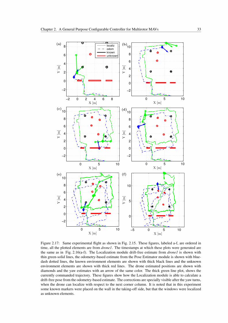
Chapter 2. A General Purpose Configurable Controller for Multirotor MAVs 33
−2 0 2 4 6 8
−2
0
2
4
6
8(a)
X [m]
Y[m
]
localiz
odom
known
unknown
0 5 10
−2
0
2
4
6
8
10(b)
X [m]
Y[m
]
0 5 10
−2
0
2
4
6
8
10(c)
X [m]
Y[m
]
0 5 10
−2
0
2
4
6
8
10(d)
X [m]
Y[m
]
0 5 10
−2
0
2
4
6
8
10(e)
X [m]
Y[m
]
−5 0 5 10
0
5
10
(f)
X [m]
Y[m
]
Figure 2.17: Same experimental flight as shown in Fig. 2.15. These figures, labeled a-f, are ordered intime, all the plotted elements are from drone1. The timestamps at which these plots were generated arethe same as in Fig. 2.16(a-f). The Localization module drift-free estimate from drone1 is shown withthin green-solid lines, the odometry-based estimate from the Pose Estimator module is shown with blue-dash dotted lines, the known environment elements are shown with thick black lines and the unknownenvironment elements are shown with thick red lines. The drone estimated positions are shown withdiamonds and the yaw estimates with an arrow of the same color. The thick green line plot, shows thecurrently commanded trajectory. These figures show how the Localization module is able to calculate adrift-free pose from the odometry-based estimate. The corrections are specially visible after the yaw turns,when the drone can localize with respect to the next corner column. It is noted that in this experimentsome known markers were placed on the wall in the taking-off side, but that the windows were localizedas unknown elements.

34 2.4. Experimental Results
20 40 60 80 100 120 140 160 180 200
0
2
4
6
8
X[m
]
xcxs
20 40 60 80 100 120 140 160 180 200
0
5
10
15
Y[m
]
ycys
20 40 60 80 100 120 140 160 180 200−2
−1
0
Z[m
]
zczs
20 40 60 80 100 120 140 160 180 2000
0.5
1
ecrosstrack
[m]
20 40 60 80 100 120 140 160 180 200
−2
0
2
time [s]
yaw
[rad]
yawcyaws
Figure 2.18: Flight performance of drone1, same experimental flight as shown in Figs. 2.15 and 2.16.The plots show the estimated position and yaw of the quadrotor and the inputs given to the position andspeed control loops inside the trajectory controller module. The ecrosstrack plot shows the absolute posi-tion control error based on these commands and the estimated position, as calculated by the localizationmodule. The yaw command only changes sharply when the drone is commanded to look at a differentcolumn. The rest of the time when a sharp change is shown it has just evolved to the opposite side of the[−π,+π] interval.

Chapter 2. A General Purpose Configurable Controller for Multirotor MAVs 35
40 60 80 100 120 140 160 180 200 220 240
0
2
4
6
8
X[m
]
xcxs
40 60 80 100 120 140 160 180 200 220 240
0
5
10
15
Y[m
]
ycys
40 60 80 100 120 140 160 180 200 220 240−2
−1
0
Z[m
]
zczs
40 60 80 100 120 140 160 180 200 220 2400
0.5
1
ecrosstrack
[m]
40 60 80 100 120 140 160 180 200 220 240
−2
0
2
time [s]
yaw
[rad]
yawcyaws
Figure 2.19: Flight performance of drone2, same experimental flight as shown in Figs. 2.15 and 2.16.The interpretation of this figure is similar to that of Fig. 2.18.

36 2.4. Experimental Results
100 150 200 250 300
0
2
4
6
8
X[m
]
xcxs
100 150 200 250 300
0
5
10
15
Y[m
]
ycys
100 150 200 250 300−2
−1
0
Z[m
]
zczs
100 150 200 250 3000
0.5
1
ecrosstrack
[m]
100 150 200 250 300
−2
0
2
time [s]
yaw
[rad]
yawcyaws
Figure 2.20: Flight performance of drone3, same experimental flight as shown in Figs. 2.15 and 2.16.The interpretation of this figure is similar to that of Fig. 2.18.
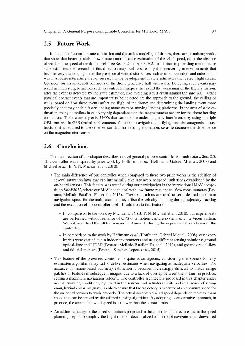
Chapter 2. A General Purpose Configurable Controller for Multirotor MAVs 37
2.5 Future WorkIn the area of control, estate estimation and dynamics modeling of drones, there are promising works
that show that better models allow a much more precise estimation of the wind speed, or, in the absenceof wind, of the speed of the drone itself, see Sec. 3.2 and Appx. E.2. In addition to providing more precisestate estimates, the research in this direction may lead to safer flight maneuvering in environments thatbecome very challenging under the presence of wind disturbances such as urban corridors and indoor hall-ways. Another interesting area of research is the development of state estimators that detect flight issues.Consider, for instance, soft collisions of the drone protective hull with walls. Detecting such events mayresult in interesting behaviors such as control techniques that avoid the worsening of the flight situation,after the event is detected by the state estimator, like avoiding a full crash against the said wall. Otherphysical contact events that are important to be detected are the approach to the ground, the ceiling orwalls, based on how these events affect the flight of the drone; and determining the landing event moreprecisely, that may enable faster landing maneuvers on moving landing platforms. In the area of state es-timation, many autopilots have a very big dependence on the magnetometer sensor for the drone headingestimation. There currently exist UAVs that can operate under magnetic interference by using multipleGPS sensors. In GPS-denied environments, for indoor navigation and flying near ferromagnetic infras-tructure, it is required to use other sensor data for heading estimation, so as to decrease the dependenceon the magnetometer sensor.
2.6 ConclusionsThe main section of this chapter describes a novel general purpose controller for multirotors, Sec. 2.3.
This controller was inspired by prior work by Hoffmann et al. (Hoffmann, Gabriel M et al., 2008) andMichael et al. (B. Y. N. Michael et al., 2010):
• The main difference of our controller when compared to these two prior works is the addition ofseveral saturation laws that can intrinsically take into account speed limitations established by theon-board sensors. This feature was tested during our participation in the international MAV compe-tition IMAV2012, where our MAV had to deal with low frame-rate optical-flow measurements (Pes-tana, Mellado-Bataller, Fu, et al., 2013). These saturations are used to set a desired maximumnavigation speed for the multirotor and they affect the velocity planning during trajectory trackingand the execution of the controller itself. In addition to this feature:
– In comparison to the work by Michael et al. (B. Y. N. Michael et al., 2010), our experimentsare performed without reliance of GPS or a motion capture system, e. g. a Vicon system.We utilize instead the EKF discussed in Annex. E during the experimental validation of thecontroller.
– In comparison to the work by Hoffmann et al. (Hoffmann, Gabriel M et al., 2008), our exper-iments were carried out in indoor environments and using different sensing solutions: groundoptical-flow and LIDAR (Pestana, Mellado-Bataller, Fu, et al., 2013), and ground optical-flowand fiducial markers (Pestana, Sanchez-Lopez, et al., 2015).
• This feature of the presented controller is quite advantageous, considering that some odometryestimation algorithms may fail to deliver estimates when navigating at inadequate velocities. Forinstance, in vision-based odometry estimation it becomes increasingly difficult to match imagepatches or features in subsequent images, due to a lack of overlap between them, thus, in practice,setting a maximum navigation velocity. The controller architecture proposed in this chapter undernormal working conditions, e.g. within the sensors and actuators limits and in absence of strongenough wind and wind-gusts, is able to ensure that the trajectory is executed at an optimum speed forthe on-board sensors to work properly. The actual acceptable wind speed depends on the maximumspeed that can be sensed by the utilized sensing algorithm. By adopting a conservative approach, inpractice, the acceptable wind speed is set lower than the sensor limits.
• An additional usage of the speed saturations proposed in the controller architecture and in the speedplanning step is to simplify the flight rules of decentralized multi-robot navigation, as showcased
38 2.6. Conclusions
in Sec. 2.4.4. This particular use of the speed saturations was utilized by the CVG_UPM during itsparticipation in the IMAV 2013 competition.
• The presented controller has been successfully utilized as part of an autonomous flight architecturein several international MAV competitions, showcasing its tested reliable implementation, and itscode has been released as open-source in github.
The main publications related to this chapter are:
• J. Pestana, J. L. Sanchez-Lopez, P. de la Puente, A. Carrio, P. Campoy. “A Vision-based QuadrotorMulti-robot Solution for the Indoor Autonomy Challenge of the 2013 International Micro Air Vehi-cle Competition”. In Journal of Intelligent and Robotic Systems, JINT2015. Springer Netherlands.
• J. Pestana, I. Mellado-Bataller, C. Fu, J. L. Sanchez-Lopez, I. F. Mondragon, P. Campoy. “AGeneral Purpose Configurable Controller for Indoors and Outdoors GPS-Denied Navigation forMultirotor Unmanned Aerial Vehicles”. In JINT2013.
• J. L. Sanchez-Lopez, J. Pestana, P. de la Puente, P. Campoy. “A reliable open-source systemarchitecture for the fast designing and prototyping of autonomous multi-uav systems: Simulationand experimentation”. In JINT2015.
• I. Mellado-Bataller, J. Pestana, M. A. Olivares-Mendez , P. Campoy, and L. Mejias, book chapter,“MAVwork: a Framework for Unified Interfacing between Micro Aerial Vehicles and Visual Con-trollers”, in book “Frontiers of Intelligent Autonomous Systems”, serie “Studies in ComputationalIntelligence Series”, Springer, 2013.
• J. Pestana, I. Mellado-Bataller, C. Fu, J. L. Sanchez-Lopez, I. F. Mondragon, P. Campoy. “Ageneral purpose configurable navigation controller for micro aerial multirotor vehicles”, In 2013International Conference on Unmanned Aircraft Systems (ICUAS), 2013.
This general purpose controller for multirotors has been used by the CVG in its participation in fiveinternational MAV competitions:
• International Micro Air Vehicle Conference and Flight Competition 2016 (IMAV 2016)9, where theCVG team was able to solve multiple tasks in fully autonomous mode and was the team to achievethe highest number of tasks, although in separate flights, in fully autonomous mode.
Despite its outstanding performance, the CVG team earned the 4th position due to the scoringsystem leaning very heavily towards the usage of very small MAVs.
• Asia Venue of the AUVSI International Aerial Robotics Competition 2014 (IARC 2014)10, sameas other teams, we were still far from achieving the interaction with the ground robots. Therefore,the CVG_UPM team showed similar capabilities to other contestants. Our level of developmentwas good as a first step towards continuing our participation the next year for IARC 2015.
• International Micro Air Vehicle Conference and Flight Competition 2013 (IMAV 2013)11, wherethe team that represented the UPM and the Computer Vision Group (CVG, UPM) was awardedwith: first place in the “Indoor Autonomy - IMAV 2013”.
• International Micro Air Vehicle Conference and Flight Competition 2012, (IMAV 2012)12, Theteam that represented the CAR and the Computer Vision Group (CVG) was twice awarded with:
– the special award “Best Automatic Performance - IMAV 2012”, as part of the overall resultsof the competitions, and
– second place in the “Indoor Flight Dynamics - Rotary Wing MAV” challenge, where the firstplace was obtained by a remotely piloted multirotor.
9IMAV 2016 video playlist: https://goo.gl/tdZyGu10IARC 2014 video playlist: https://goo.gl/bEvK3F11IMAV 2013 video playlist: https://goo.gl/KosWKH12IMAV 2012 video playlist: https://goo.gl/PRns2D

Chapter 2. A General Purpose Configurable Controller for Multirotor MAVs 39
• Contest on Control Engineering 2012, (IC CEA 2012), organized by the Spanish Committee ofAutomation. Two teams participated representing the Universidad Politécnica de Madrid (UPM)and the Computer Vision Group (CVG_UPM), and were awarded with:
– Undergraduate students’ of the ETSII-UPM engineering school using their own developedsoftware supervised by J. Pestana: the first (phase 1 - simulation) and third places (final phase- autonomous flight event)
– CVG PhD students’ team, using the presented controller: the second (phase 1 - simulation)and fifth places (final phase - autonomous flight event). In the final phase of the competitionour team achieved the fifth place, due to our controller, when compared to other teams, leaningtowards low tracking error with higher round-trip times.
The source of this controller has been released as open-source as part of the stack for the control ofmultirotor MAVs from the CVG, first integrated to MAVwork1314 and currently as part of Aerostack1516.
This controller has been showcased in several live demos by the CVG (UPM):
• CivilDRON 2017 congress17, Madrid (Spain)Simplified version of IMAV 2016 competition missionJanuary 2017
• CivilDRON 2016 congress18, Madrid (Spain)Multi-robot mission and vision-based person followingMay 2016
• Semana de la Ciencia 2015 - Science Week 20151920, Madrid (Spain)Multi-robot mission and vision-based person followingNovember 2-15, 2015
• Noche Europea de los investigadores - European Researchers’ Night 201521
Multi-robot mission, vision-based person following and a simple search and rescue mission, whichincluded the usage of a multi-modal human-machine interface with the MAV.Madrid (Spain), September 2015
• Semana de la Ciencia 2014 - Science Week 201422, Madrid (Spain)Multi-robot mission and vision-based person followingNovember 2014
• Semana de la Ciencia 2013 - Science Week 201323, Madrid (Spain)Multi-robot mission and vision-based person followingNovember 4-17, 2013
13Git repository: https://github.com/uavster/mavwork14Git repository: https://github.com/jespestana/MultirotorController4mavwork15Git repository: https://github.com/Vision4UAV/cvg_quadrotor_swarm16Git repository: https://github.com/Vision4UAV/Aerostack17CivilDRON 2017: http://www.civildron.com/18CivilDRON 2016: http://www.aerpas.es/wp-content/uploads/2015/04/CivilDRON16_v2.pdf19Semana de la Ciencia 2015 - Website:http://bit.ly/2lN9RNg20Semana de la Ciencia 2015 - Results Report:http://bit.ly/2muELHG21European Researchers’ Night 2015 - Website: http://bit.ly/2mM6a9Q22Semana de la Ciencia 2014 - Results Report:http://bit.ly/2lNg1NA23Semana de la Ciencia 2013 - Results Report:http://bit.ly/2npz2lF

40 2.7. Chapter Bibliography
2.7 Chapter BibliographyAchtelik, M., Bachrach, A., He, R., Prentice, S., and Roy, N. (2009). “Stereo vision and laser odometry
for autonomous helicopters in GPS-denied indoor environments”. In: SPIE Defense, Security, andSensing. International Society for Optics and Photonics, pp. 733219–733219 (cit. on p. 11).
Agrachev, A. A. and Sachkov, Y. (2004). Control theory from the geometric viewpoint. Vol. 2. SpringerScience & Business Media (cit. on p. 12).
Bachrach, A. G. (2009). “Autonomous flight in unstructured and unknown indoor environments”. MAthesis. Massachusetts Institute of Technology (cit. on p. 11).
Bachrach, A., Prentice, S., He, R., and Roy, N. (2011). “RANGE-Robust autonomous navigation in GPS-denied environments”. Journal of Field Robotics 28.5, pp. 644–666 (cit. on p. 11).
Bouabdallah, S., Murrieri, P., and Siegwart, R. (2005). “Towards autonomous indoor micro VTOL”. Au-tonomous Robots 18.2, pp. 171–183 (cit. on p. 12).
Bouabdallah, S. and Siegwart, R. (2005). “Backstepping and sliding-mode techniques applied to an indoormicro quadrotor”. In: Robotics and Automation, 2005. ICRA 2005. Proceedings of the 2005 IEEEInternational Conference on. IEEE, pp. 2247–2252 (cit. on p. 12).
Bristeau, P.-J., Callou, F., Vissiere, D., Petit, N., et al. (2011). “The navigation and control technologyinside the ar. drone micro uav”. In: 18th IFAC World Congress. Vol. 18, pp. 1477–1484 (cit. on p. 23).
Castillo, P., Dzul, A., and Lozano, R. (2004). “Real-time stabilization and tracking of a four-rotor minirotorcraft”. Control Systems Technology, IEEE Transactions on 12.4, pp. 510–516 (cit. on p. 12).
Castillo, P., Lozano, R., and Dzul, A. (2005). “Stabilization of a mini rotorcraft with four rotors”. IEEEControl Systems Magazine 25.6, pp. 45–55 (cit. on p. 12).
Cowling, I. D., Yakimenko, O. A., Whidborne, J. F., and Cooke, A. K. (2010). “Direct method basedcontrol system for an autonomous quadrotor”. Journal of Intelligent & Robotic Systems 60.2, pp. 285–316 (cit. on p. 12).
Mellado Bataller, I. (2012). A new framework for interfacing with MAVs. https://github.com/uavster/mavwork (cit. on p. 13).
Driessen, B. J. and Robin, A. L. (2004). “A globally convergent tracking controller for the X4 flyer rotorcraft for reference trajectories with positive thrust”. Robotica 22.04, pp. 375–388 (cit. on p. 12).
Fritsch, O., De Monte, P., Buhl, M., and Lohmann, B. (2012). “Quasi-static feedback linearization forthe translational dynamics of a quadrotor helicopter”. In: American Control Conference (ACC), 2012.IEEE, pp. 125–130 (cit. on p. 12).
Garrido-Jurado, S., Muñoz-Salinas, R., Madrid-Cuevas, F. J., and Marín-Jiménez, M. J. (2014). “Auto-matic generation and detection of highly reliable fiducial markers under occlusion”. Pattern Recogni-tion 47.6, pp. 2280–2292 (cit. on p. 27).
Gillula, J. H., Huang, H., Vitus, M. P., and Tomlin, C. J. (2010). “Design of Guaranteed Safe ManeuversUsing Reachable Sets : Autonomous Quadrotor Aerobatics in Theory and Practice”. IEEE ElectricalEngineering (2010), pp. 1649–1654 (cit. on p. 11).
Guenard, N., Hamel, T., and Moreau, V. (2005). “Dynamic modeling and intuitive control strategy for an"X4-flyer"”. In: Control and Automation, 2005. ICCA’05. International Conference on. Vol. 1. IEEE,pp. 141–146 (cit. on p. 12).
Heng, L., Honegger, D., Lee, G. H., Meier, L., Tanskanen, P., Fraundorfer, F., and Pollefeys, M. (2014).“Autonomous visual mapping and exploration with a micro aerial vehicle”. Journal of Field Robotics31.4, pp. 654–675 (cit. on p. 11).
Hoffmann, Gabriel M, Waslander, Steven L, and Tomlin, Claire J (2008). “Quadrotor Helicopter Trajec-tory Tracking Control”. Electrical Engineering (2008), pp. 1–14 (cit. on pp. 11, 12, 16, 18, 37).
Hoffmann, G.M., Waslander, S.L., and Tomlin, C.J. (2009). “Aerodynamics and control of autonomousquadrotor helicopters in aggressive maneuvering”. In: 2009 IEEE International Conference onRobotics and Automation. Ieee, pp. 3277–3282 (cit. on pp. 11, 12).
Hoffmann, G. M., Huang, H., Waslander, S. L., and Tomlin, C. J. (2007). “Quadrotor helicopter flightdynamics and control: Theory and experiment”. In: Proc. of the AIAA Guidance, Navigation, andControl Conference. Vol. 2 (cit. on p. 12).
Hoffmann, G. M., Waslander, S. L., and Tomlin, C. J. (2006). “Distributed Cooperative Search usingInformation-Theoretic Costs for Particle Filters , with Quadrotor Applications”. Electrical Engineer-ing, pp. 1–21 (cit. on pp. 11, 12).

Chapter 2. A General Purpose Configurable Controller for Multirotor MAVs 41
Hua, M.-D., Hamel, T., Morin, P., and Samson, C. (2009). “A control approach for thrust-propelled un-deractuated vehicles and its application to VTOL drones”. Automatic Control, IEEE Transactions on54.8, pp. 1837–1853 (cit. on p. 12).
Huang, A. S., Bachrach, A., Henry, P., Krainin, M., Fox, D., and Roy, N. (2011). “Visual Odometry andMapping for Autonomous Flight Using an RGB-D Camera”. Camera (cit. on p. 11).
Jurdjevic, V. (1997). Geometric control theory. Cambridge university press (cit. on p. 12).Kendoul, F., Yu, Z., and Nonami, K. (2010). “Guidance and nonlinear control system for autonomous
flight of minirotorcraft unmanned aerial vehicles”. Journal of Field Robotics 27.3, pp. 311–334 (cit.on p. 12).
Kushleyev, A., Kumar, V., and Mellinger, D. (2012). “Towards A Swarm of Agile Micro Quadrotors”. In:Proceedings of Robotics: Science and Systems. Sydney, Australia (cit. on p. 11).
Lee, D., Kim, H. J., and Sastry, S. (2009). “Feedback linearization vs. adaptive sliding mode control fora quadrotor helicopter”. International Journal of control, Automation and systems 7.3, pp. 419–428(cit. on p. 12).
Lee, T., Leoky, M., and McClamroch, N. H. (2010). “Geometric tracking control of a quadrotor UAVon SE (3)”. In: Decision and Control (CDC), 2010 49th IEEE Conference on. IEEE, pp. 5420–5425(cit. on p. 12).
Lippiello, V., Loianno, G., and Siciliano, B. (2011). “MAV indoor navigation based on a closed-formsolution for absolute scale velocity estimation using Optical Flow and inertial data”. In: Decision andControl and European Control Conference (CDC-ECC), 2011 50th IEEE Conference on, pp. 3566–3571 (cit. on p. 12).
Madani, T. and Benallegue, A. (2007). “Backstepping control with exact 2-sliding mode estimation for aquadrotor unmanned aerial vehicle”. In: Intelligent Robots and Systems, 2007. IROS 2007. IEEE/RSJInternational Conference on. IEEE, pp. 141–146 (cit. on p. 12).
Mellado-Bataller, I., Mejias, L., Campoy, P., and Olivares-Mendez, M. A. (2012). “Rapid prototypingframework for visual control of autonomous micro aerial vehicles”. In: 12th International Conferenceon Intelligent Autonomous System (IAS-12). Jeju Island, Korea (cit. on p. 13).
Mellado-Bataller, I., Pestana, J., Olivares-Mendez, M. A., Campoy, P., and Mejias, L. (2013). “MAVwork:a framework for unified interfacing between micro aerial vehicles and visual controllers”. In: Frontiersof Intelligent Autonomous Systems. Springer, pp. 165–179 (cit. on p. 13).
Mellinger, D., Michael, N., and Kumar, V. (2010). “Trajectory Generation and Control for Precise Ag-gressive Maneuvers with Quadrotors”. In: Int Symposium on Experimental Robotics (2010) (cit. onpp. 11, 12, 16).
Michael, B. Y. N., Mellinger, D., and Lindsey, Q. (2010). “The GRASP Multiple Micro UAV Testbed”.IEEE Robotics & Automation Magazine, pp. 56–65 (cit. on pp. 11, 12, 16, 37).
Michael, N., Shen, S., Mohta, K., Mulgaonkar, Y., Kumar, V., Nagatani, K., Okada, Y., Kiribayashi, S.,Otake, K., Yoshida, K., et al. (2012). “Collaborative mapping of an earthquake-damaged building viaground and aerial robots”. Journal of Field Robotics 29.5, pp. 832–841 (cit. on p. 11).
Mistler, V., Benallegue, A., and M’sirdi, N. (2001). “Exact linearization and noninteracting control of a4 rotors helicopter via dynamic feedback”. In: Robot and Human Interactive Communication, 2001.Proceedings. 10th IEEE International Workshop on. IEEE, pp. 586–593 (cit. on p. 12).
Nice, E. B. (2004). “Design of a four rotor hovering vehicle”. PhD thesis. Cornell University (cit. onp. 12).
Pestana, J., Mellado-Bataller, I., Fu, C., Sanchez-Lopez, J. L., Mondragon, I. F., and Campoy, P. (2013).“A general purpose configurable navigation controller for micro aerial multirotor vehicles”. In: Un-manned Aircraft Systems (ICUAS), 2013 International Conference on. IEEE, pp. 557–564 (cit. onpp. 18, 19, 37).
Pestana, J., Mellado-Bataller, I., Sanchez-Lopez, J. L., Fu, C., Mondragón, I. F., and Campoy, P. (2014).“A general purpose configurable controller for indoors and outdoors gps-denied navigation for multi-rotor unmanned aerial vehicles”. Journal of Intelligent & Robotic Systems 73.1-4, pp. 387–400 (cit. onpp. 19, 22).
Pestana, J., Sanchez-Lopez, J. L., Puente, P. de la, Carrio, A., and Campoy, P. (2015). “A Vision-basedQuadrotor Multi-robot Solution for the Indoor Autonomy Challenge of the 2013 International MicroAir Vehicle Competition”. Journal of Intelligent & Robotic Systems, pp. 1–20 (cit. on pp. 19, 27, 37).
Quaritsch, M., Stojanovski, E., Bettstetter, C., Friedrich, G., Hellwagner, H., Rinner, B., Hofbaur, M.,and Shah, M. (2008). “Collaborative Microdrones: Applications and Research Challenges”. In: Pro-

42 2.7. Chapter Bibliography
ceedings of the Second International ICST Conference on Autonomic Computing and CommunicationSystems. Gent, BELGIUM: Icst (cit. on p. 11).
Raffo, G. V., Ortega, M. G., and Rubio, F. R. (2010). “An integral predictive/nonlinear Hinf controlstructure for a quadrotor helicopter”. Automatica 46.1, pp. 29–39 (cit. on p. 12).
Richter, Charles, Bry, Adam, and Roy, Nicholas (2013). “Polynomial trajectory planning for aggressivequadrotor flight in dense indoor environments”. In: Proceedings of the International Symposium onRobotics Research (ISRR) (cit. on p. 12).
Rudol, P., Wzorek, M., Conte, G., and Doherty, P. (2008). “Micro unmanned aerial vehicle visual servoingfor cooperative indoor exploration”. In: Aerospace, 2008 IEEE Conference on (cit. on p. 12).
S., L., A., S., M, S., and D’Andrea, R. (2010). “A Simple Learning Strategy for High-Speed QuadrocopterMulti-Flips”. In: 2010 IEEE International Conference on Robotics and Automation (ICRA 2010),pp. 1642–1648 (cit. on p. 11).
Scaramuzza, D., Achtelik, M., Doitsidis, L., Fraundorfer, F., Kosmatopoulos, E., Martinelli, A., et al.(2013). “Vision-controlled micro flying robots: from system design to autonomous navigation andmapping in gps-denied environments”. IEEE Robotics and Automation Magazine (cit. on p. 11).
Schölling, A., Augugliaro, F., Lupashin, S., and D’Andrea, R. (2010). “Synchronizing the Motion ofa Quadrocopter to Music”. In: IEEE International Conference on Robotics and Automation ICRA,pp. 3355–3360 (cit. on p. 11).
Shen, Shaojie, Mulgaonkar, Yash, Michael, Nathan, and Kumar, Vijay (2013). “Vision-based state estima-tion for autonomous rotorcraft mavs in complex environments”. In: Robotics and Automation (ICRA),2013 IEEE International Conference on. IEEE, pp. 1758–1764 (cit. on p. 12).
Shen, S., Michael, N., and Kumar, V. (2011). “Autonomous multi-floor indoor navigation with a compu-tationally constrained MAV”. Robotics and Automation (ICRA), 2011 IEEE International Conferenceon, pp. 20–25 (cit. on p. 11).
Shen, S., Mulgaonkar, Y., Michael, N., and Kumar, V. (2013). “Vision-Based State Estimation and Tra-jectory Control Towards High-Speed Flight with a Quadrotor.” In: Robotics: Science and Systems.Citeseer (cit. on p. 12).
(2012). The Stanford/Berkeley Testbed of Autonomous Rotorcraft for Multi-Agent Control (STARMAC)project. http://hybrid.eecs.berkeley.edu/starmac/ (cit. on p. 11).
Valenti, M., Bethke, B., Fiore, G., How, J. P., and Feron, E. (2006). “Indoor multi-vehicle flight testbedfor fault detection, isolation, and recovery”. In: Proceedings of the AIAA Guidance, Navigation, andControl Conference and Exhibit, Keystone, CO. Vol. 63, p. 64 (cit. on p. 12).
Weiss, S., Achtelik, M. W., Chli, M., and Siegwart, R. (2012). “Versatile distributed pose estimation andsensor self-calibration for an autonomous MAV”. In: Robotics and Automation (ICRA), 2012 IEEEInternational Conference on. IEEE, pp. 31–38 (cit. on p. 11).
Zingg, S., Scaramuzza, D., Weiss, S., and Siegwart, R. (2010). “MAV Navigation through Indoor Corri-dors Using Optical Flow”. In: Robotics and Automation (ICRA), 2010 IEEE International Conferenceon (cit. on p. 12).
Zufferey, J.-C., Beyeler, A., and Floreano, D. (2010). “Autonomous flight at low altitude with vision-based collision avoidance and GPS-based path following”. In: Proceedings of the IEEE InternationalConference on Robotics and Automation (ICRA). Anchorage, Alaska: IEEE (cit. on p. 12).
Chapter 3Visual Servoing of Arbitrary Objectsfor Multirotors
3.1 IntroductionThis research showcases visual object tracking for Unmanned Air Vehicles (UAV) to perform GPS-
denied object following tasks, on a big variety of objects in outdoors suburban environments. Navigationis more challenging for a flying robot than for ground robots because it requires feedback to stabilizeitself. This fact provides a second objective, which is to show that visual servoing or visual based objectfollowing is possible and reliable for a great variety of objects. The capability of autonomous tracking andfollowing of arbitrary objects is interesting by itself; because it can be directly applied to visual inspectionamong other civilian tasks. So far, this work has been a feasibility project to showcase the possibilitiesof visual servoing to operate in relatively spacious unknown outdoors environments in suburban areas.The proposed architecture addresses these objectives through the knowledgeable choice of robust reliablecomponents, namely: the open-source object tracker OpenTLD (Kalal, 2011; Kalal et al., 2012), and theAR Drone 2.0 (see Fig. 3.1-left).
The Vertical Take-Off and Landing (VTOL) UAV platform used in the experimental work is the mul-tirotor Parrot AR.Drone 2.0, shown in Figs. 3.1 & 3.2. Recent research has demonstrated that the theAR Drone is a realiable platform for VTOL UAV vision based navigation algorithm prototyping. Forinstance, the AR Drone has been used on the following research: autonomous navigation of hallwaysand stairs (Bills et al., 2011), visual SLAM based navigation (Engel et al., 2012) and reactive obstacleavoidance in natural environments (Ross et al., 2013).
The AR Drone 2 platform was selected for experimental testing of the presented work for multiplereasons: it is practically harmless to people and third-party objects, its ease of use thanks to its built-inflying modes, its low price, and its robustness to crashes. Since one of the main objectives of the presentedresearch work was to perform person following from close distances, the chosen multirotor platform hadto be safe to fly close to people.
This work is a continuation of previous work by the CVG group (Mondragoón et al., 2011) where
43
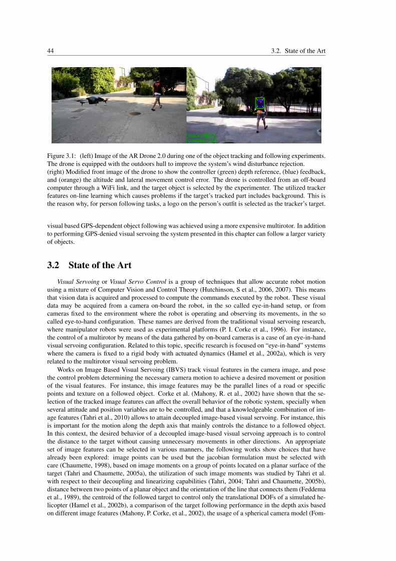
44 3.2. State of the Art
Figure 3.1: (left) Image of the AR Drone 2.0 during one of the object tracking and following experiments.The drone is equipped with the outdoors hull to improve the system’s wind disturbance rejection.(right) Modified front image of the drone to show the controller (green) depth reference, (blue) feedback,and (orange) the altitude and lateral movement control error. The drone is controlled from an off-boardcomputer through a WiFi link, and the target object is selected by the experimenter. The utilized trackerfeatures on-line learning which causes problems if the target’s tracked part includes background. This isthe reason why, for person following tasks, a logo on the person’s outfit is selected as the tracker’s target.
visual based GPS-dependent object following was achieved using a more expensive multirotor. In additionto performing GPS-denied visual servoing the system presented in this chapter can follow a larger varietyof objects.
3.2 State of the ArtVisual Servoing or Visual Servo Control is a group of techniques that allow accurate robot motion
using a mixture of Computer Vision and Control Theory (Hutchinson, S et al., 2006, 2007). This meansthat vision data is acquired and processed to compute the commands executed by the robot. These visualdata may be acquired from a camera on-board the robot, in the so called eye-in-hand setup, or fromcameras fixed to the environment where the robot is operating and observing its movements, in the socalled eye-to-hand configuration. These names are derived from the traditional visual servoing research,where manipulator robots were used as experimental platforms (P. I. Corke et al., 1996). For instance,the control of a multirotor by means of the data gathered by on-board cameras is a case of an eye-in-handvisual servoing configuration. Related to this topic, specific research is focused on “eye-in-hand” systemswhere the camera is fixed to a rigid body with actuated dynamics (Hamel et al., 2002a), which is veryrelated to the multirotor visual servoing problem.
Works on Image Based Visual Servoing (IBVS) track visual features in the camera image, and posethe control problem determining the necessary camera motion to achieve a desired movement or positionof the visual features. For instance, this image features may be the parallel lines of a road or specificpoints and texture on a followed object. Corke et al. (Mahony, R. et al., 2002) have shown that the se-lection of the tracked image features can affect the overall behavior of the robotic system, specially whenseveral attitude and position variables are to be controlled, and that a knowledgeable combination of im-age features (Tahri et al., 2010) allows to attain decoupled image-based visual servoing. For instance, thisis important for the motion along the depth axis that mainly controls the distance to a followed object.In this context, the desired behavior of a decoupled image-based visual servoing approach is to controlthe distance to the target without causing unnecessary movements in other directions. An appropriateset of image features can be selected in various manners, the following works show choices that havealready been explored: image points can be used but the jacobian formulation must be selected withcare (Chaumette, 1998), based on image moments on a group of points located on a planar surface of thetarget (Tahri and Chaumette, 2005a), the utilization of such image moments was studied by Tahri et al.with respect to their decoupling and linearizing capabilities (Tahri, 2004; Tahri and Chaumette, 2005b),distance between two points of a planar object and the orientation of the line that connects them (Feddemaet al., 1989), the centroid of the followed target to control only the translational DOFs of a simulated he-licopter (Hamel et al., 2002b), a comparison of the target following performance in the depth axis basedon different image features (Mahony, P. Corke, et al., 2002), the usage of a spherical camera model (Fom-

Chapter 3. Visual Servoing of Arbitrary Objects for Multirotors 45
ena et al., 2007), projecting image features into the unit sphere and using them in the control law (Tahri,Chaumette, and Mezouar, 2008), and also even projecting the triangle surfaces between image featuresinto the unit sphere (Tahri et al., 2009). Interestingly, recent research has included non-overlapping multi-camera robotic systems (Comport et al., 2011).
The visual servoing strategy con be modified to avoid following non-straight or far-away image featureposition references, by defining desired feature-paths using different techniques: including the nonlinearminimization methods to select the desired image feature path on the image plane based on a Hessiancalculation (Lapresté et al., 2004; Malis, 2004; Tahri and Mezouar, 2010); a combination of path planningand visual servoing allows to perform longer camera displacements around the target while keeping thetarget in the field of view of the camera and respecting the joint limits of the robot (Chesi and Vicino,2004; Mezouar et al., 2002), including big orientation reference changes (Schramm et al., 2007), and alsoto avoid obstacles during object tracking (Chesi, 2009).
Different research work has been done where a vision system with range sensors was used for ObjectFollowing tasks. On (Argyros et al., 2002) an omnidirectional visual system was used as a bearing sensor,while the distance to the target is measured using a range sensor, for control a robotic wheelchair on in-doors. Others systems have been proposed only based on visual information for cooperative robotics (Ko-rodi et al., 2008).
Visual information have been exploited on many projects involving UAVs, for instance to allow: fixedwing UAVs to fly at a constant altitude following a moving object on a ground planar surface (Fahd Rafi etal., 2006; Savkin et al., 2008), rotary wing UAVs to follow a terrestrial target (Deng et al., 2009; Lin et al.,2010), pose-based methods for autonomous landing on moving objects (Saripalli et al., 2007), and GPSdependent visual servoing for low altitude moving targets (Mondragoón et al., 2011). Also, recent workon visual based navigation using monocular SLAM methods for indoors environment has been achievedwith promising results (Achtelik et al., 2011; Engel et al., 2012).
Recent research on Visual Tracking has been focused on online learning and detection algo-rithms (Babenko et al., 2009; Kalal et al., 2012). Such trackers have demonstrated to be able to tracka wide variety of targets in real-time. When compared to prior research, the main advantage of the UAVVisual Servoing system proposed in this Thesis is that we use a tracker, OpenTLD, which allows to per-form visual servoing with a large number of different targets. Our proposed architecture addresses theseobjectives through the knowlegeable choice of robust reliable components, namely: the open-source ob-ject tracker OpenTLD (Kalal, 2011; Kalal et al., 2012), and the AR Drone 2.0. Following arbitrarilychosen targets is a big improvement compared to following targets marked with blobs of different sizes,which is a commonly used target to measure the performance of visual servoing controllers, see for in-stance (Bourquardez et al., 2009) or (Espiau et al., 1992), or when compared to following balloons usingcolor based tracking (Mondragoón et al., 2011; Zhang et al., 1999). However, our architecture is not ableto estimate the depth at which the target is located as in (Mahony, Brasch, et al., 2005), or the relativeattitude of the target with respect to the drone, as in (Martínez et al., 2013).
Other works have focused on developing image trackers designed with UAV object following in mind.Teuliere et al. (Teuliere et al., 2011) propose using a color based tracker using a multi-part representationof the followed target using particle filter based estimation. Danelljan et al. (Danelljan, Khan, et al., 2014;Danelljan, Shahbaz Khan, et al., 2014) used a novel color based tracking method and a combination ofstate of the art filtering and Artificial Intelligence (AI) algorithms to achieve person following and multi-person visual tracking. Haag. et al. (Haag et al., 2015) proposed a novel visual-based tracker to follow aperson and tested it on various following scenarios, like walking at different speeds or riding a bike.
Road following and corridor navigation tasks by UAVs have also received attention. A commonlyreferenced work for including computer vision directly in a control loop where only visual features areused as measurements and control references was done by Espiau et al. (Espiau et al., 1992), whichincluded experiments on target and road following. A road following task by an airship which followsthe horizon line and a vanishing point on the image plane was proposed by Rives et al. (Rives et al.,2004). Bills et al. (Bills et al., 2011) proposed using a CV classifier to determine the type of indoorenvironment where an quadrotor is navigating, and then used this information to control the UAV basedon perspective cues specifically tailor to the detected environment such as the perspective vanishing point.Ross et al. (Ross et al., 2013) used visual cues for achieving relatively safe UAV flight in forests byavoiding trees on the direction of navigation using a reactive control law.

46 3.3. System Description
3.3 System Description
Our system consists of several modules which communicate with each other under the Robot Oper-ating System (ROS) framework (Quigley et al., 2009). The main modules of our system are an objecttracker and an Image Based Visual Servoing IBVS controller. As shown in Fig. 3.3, the AR.Drone 2.0 iscommanded from a computer via WiFi link using the ardrone_autonomy ROS package (Mani Monajjemi,2012).
Figure 3.2: (left) Parrot AR.Drone 2.0 and its body reference frame, {Xm, Ym, Zm}. Xm points towardsthe front of the vehicle, Ym points towards the right and Zm points downwards, obtaining an orthonormalright-handed reference frame. The attitude is defined using Euler angles, which are denoted {φ , roll},{θ ,pitch} and {ψ,yaw}.(right) While performing the visual servoing tasks the drone tracks the target from a constant distance.The target’s relative position, [∆xtm,∆ytm,∆ztm], is estimated from the image feedback using an expectedtarget’s size value, Aexp. ψtelemre f is a variable internal yaw reference which specifies the prefered relativetracking direction.
The following is a brief description of each of the modules:
1. Object tracker: our software is currently using a C++ open-source implementation of the OpenTLDtracker (Nebehay, 2012). The OpenTLD tracker was originally developed by Z. Kalal at the Uni-versity of Surrey during his PhD Thesis (Kalal, 2011; Kalal et al., 2012). The repositories relatedto this library can be found in (Kalal, Z, 2011; Nebehay, G, 2012; Chauvin, R, 2012).
OpenTLD can robustly track objects in the drone’s video stream without any previous knowledge ofthe target. The tracker feeds back a bounding box (location, height and width) around the trackedobject along with a confidence ratio. OpenTLD was tested during flight with a great variety ofobjects, see the objects shown in Figs. 3.6 & 3.7 & 3.11 & 3.14. The only constraints that weredetermined to be important to get high repeatability during testing were that: the tracker’s learningfeature has to be switched off to enable the target occlusion capability, and small targets require thebounding box not to include any background.
2. IBVS controller: the controller closes four feedback loops based on three image features, whichare the target’s bounding box centroid and size, see Fig. 3.4. The references to the controller are itsdesired values. The resulting system’s behavior is that the drone will turn to look at the target andapproximately control its relative position with regards to it.
As a result of the above mentioned system architecture, the sensor information required during theexperiments is, see Fig. 3.4:
1. During successful object tracking: the built-in operation of the drone requires, at all times, to use theIMU and the ultrasound altitude sensor. Additionally, our off-board software uses the front cameraimage and part of the IMU telemetry data. Since the AR Drone is executing its internal “flyingmode”, it does not use optical flow based speed estimation during the execution of this operationmode of our architecture.
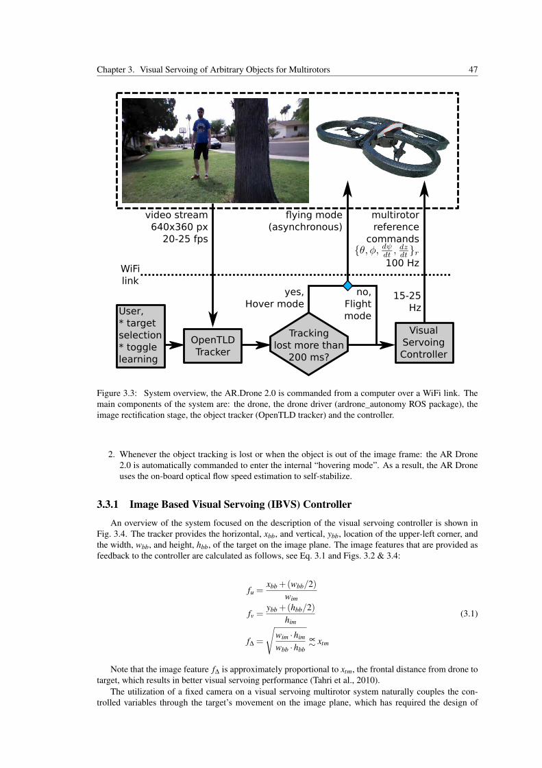
Chapter 3. Visual Servoing of Arbitrary Objects for Multirotors 47
video stream640x360 px
20-25 fps
WiFilink
OpenTLDTracker
User,* targetselection* togglelearning
Trackinglost more than
200 ms?
Visual ServoingController
yes, Hover mode
no,Flightmode
flying mode(asynchronous)
15-25 Hz
multirotorreference
commands
100 Hz
Figure 3.3: System overview, the AR.Drone 2.0 is commanded from a computer over a WiFi link. Themain components of the system are: the drone, the drone driver (ardrone_autonomy ROS package), theimage rectification stage, the object tracker (OpenTLD tracker) and the controller.
2. Whenever the object tracking is lost or when the object is out of the image frame: the AR Drone2.0 is automatically commanded to enter the internal “hovering mode”. As a result, the AR Droneuses the on-board optical flow speed estimation to self-stabilize.
3.3.1 Image Based Visual Servoing (IBVS) Controller
An overview of the system focused on the description of the visual servoing controller is shown inFig. 3.4. The tracker provides the horizontal, xbb, and vertical, ybb, location of the upper-left corner, andthe width, wbb, and height, hbb, of the target on the image plane. The image features that are provided asfeedback to the controller are calculated as follows, see Eq. 3.1 and Figs. 3.2 & 3.4:
fu =xbb +(wbb/2)
wim
fv =ybb +(hbb/2)
him(3.1)
f∆ =
√wim ·him
wbb ·hbb∝∼ xtm
Note that the image feature f∆ is approximately proportional to xtm, the frontal distance from drone totarget, which results in better visual servoing performance (Tahri et al., 2010).
The utilization of a fixed camera on a visual servoing multirotor system naturally couples the con-trolled variables through the target’s movement on the image plane, which has required the design of

48 3.3. System Description
Attitude& HeightControl
Built-in On-Board software
User interaction:* target selection* toggle learning* IBVS references:
FlightMode
Hovering IMU,magnetometer,
ultrasound altitude sensor
PositionHold
Control
Optical flowbased speedestimation
ImageRectification
Object Tracker
WiFilink
IBVS Controller
PD
Contr
olle
rs
Deco
up
ling
heuri
stic
s
Figure 3.4: Diagram of the Image Based Visual Servoing (IBVS) Controller. Since the tracker is work-ing properly at this moment, the drone is operating under the flight mode and following the drone ref-erence commands that the off-board computer is sending via WiFi. During flight mode, the optical flowspeed estimation is unused. The figure shows the image features utilized by the controller, which are:{ fu, fv ∈ [0,1]} related to the centroid position and { f∆ > 0} to the size of the bounding box.
decoupling control heuristics for the altitude and lateral movement degrees of freedom. Thus, the cor-rection shown on Eq. 3.2 on the tracking error is calculated, which greatly decreases the mentioned DOFcouplings. The terms related to the decoupling control heuristics for the image features and the DOFs ofthe quadrotor are the two terms specified on the right side of Eq. 3.2.
∆ fuψ = ∆ fu
∆ fuy = ∆ fu−ψtelemre f −ψtelem
FOVu(3.2)
∆ fvz = ∆ fv−θcentroid re f −θtelem
FOVv∆ f∆x = ∆ f∆
θtelem and ψtelem are the pitch and yaw angles of the vehicle respectively, as shown in Fig. 3.2, whichare obtained from the AR Drone telemetry data. FOVu and FOVv denote the horizontal and vertical fieldof view of the camera. ψtelemre f is a yaw heading reference which is updated to ψtelem everytime that thedrone is commanded to enter the Flight Mode or whenever |ψtelemre f − ψtelem| > 25◦. θcentroid re f isalways 0.0, and θtelem is obtained from the drone’s telemetry data.
3.3.2 IBVS PD Controller Parameters BreakdownIn this subsection the controller gains are decomposed, see Fig. 3.5, in parameters related to various
system components: process of image formation on the camera, a previously tunned position controller;

Chapter 3. Visual Servoing of Arbitrary Objects for Multirotors 49
targetdependent
cameracalibration
positioncontroller
modelidentification
Figure 3.5: IBVS Controller Breakdown, the PD controllers shown in Fig. 3.4 can be de-composed to show how they relate to a regular position controller. The shown parameterscome from: the camera parameters, the expected target size Aexp and distance to the targetdexp, the position controller gains and the aerodynamic friction of the vehicle. The obtainedPD gains are: {PD fu→ytm , K p =−0.298, Kd =−0.145}, {PD fu→∆ψ , K p =−0.990, Kd =−0.119},{PD fv→ztm , K p = 1.430, Kd = 0.371}, {PD f∆x→xtm , K p = 0.0254, Kd = 0.0124}, for the following ARDrone command gains configuration: {θr = 1→ 12◦}, {φr = 1→ 12◦}, { dψr
dt = 1→ 100 degs }, { dz
dt = 1→1 m
s }.
and the stationary relationship between speeds and drone reference commands. This decomposition al-lows to understand the effect that each parameter can have on the overall behaviour of the system duringthe Visual Servoing task.
The meaning of the the constants in Fig. 3.5 is:
• The target dependent parameters are the size of the tracked object’s target surface,Aexp = 40×30 cm; and the expected distance to the target dexp = 3 m.
• The camera dependent parameters are: the image resolution along width wim and height him; thefocal length measured in pixels αu, αv; and the horizontal field of view of the camera, FOVu,obtained from the rectified image projection matrix P, see Eq. 3.3:
P =
αu 0 u0 00 αv v0 00 0 1 0
(3.3)
• {∆xtme,∆ytme,∆ztme,∆ψtme} is the estimated relative position of the target with respect to the drone,expressed in the drone’s reference frame, as shown in Fig. 3.2.
{∆vxmr,∆vymr
}are speed commands
in the same reference frame.
• PDvar1→var2 are the PD controllers of an already tunned position controller which outputs speedcommands. For the experimental work the position controller presented in (Pestana, Mellado-Bataller, et al., 2013), and Sec. 2, was used.
•{
kθ→vx ,kφ→vy
}, are the static relationship between the multirotor tilt and the attained horizontal
steady-state speed. In multirotors this constant is related to the aerodynamic profile of the vehicle.Using the methodology presented in (Pestana, 2012), and Appx. D, for the AR Drone with theoutdoors hull, they were estimated to be ktilt→vxy ≈ 5−7m/s
24◦ for angles lower than 12◦.
•{
θr,φr,dψrdt ,
dzdt
}are the reference commands, Fig. 3.4.
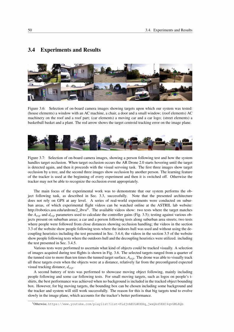
50 3.4. Experiments and Results
3.4 Experiments and Results
Figure 3.6: Selection of on-board camera images showing targets upon which our system was tested:(house elements) a window with an AC machine, a chair, a door and a small window; (roof elements) ACmachinery on the roof and a roof part; (car elements) a moving car and a car logo; (street elements) abasketball basket and a plant. The red arrow shows the target centroid tracking error on the image plane.
Figure 3.7: Selection of on-board camera images, showing a person following test and how the systemhandles target occlusion. When target occlusion occurs the AR Drone 2.0 starts hovering until the targetis detected again, and then it proceeds with the visual servoing task. The first three images show targetocclusion by a tree, and the second three images show occlusion by another person. The learning featureof the tracker is used at the beginning of every experiment and then it is switched off. Otherwise thetracker may not be able to recognize the occlusion event appropriately.
The main focus of the experimental work was to demonstrate that our system performs the ob-ject following task, as described in Sec. 3.3, successfully. Note that the presented architecturedoes not rely on GPS at any level. A series of real-world experiments were conducted on subur-ban areas, of which experimental flight videos can be watched online at the ASTRIL lab website:http://robotics.asu.edu/ardrone2_ibvs/1. The available videos show: two tests where the target matchesthe Aexp and dexp parameters used to calculate the controller gains (Fig. 3.5); testing against various ob-jects present on suburban areas; a car and a person following tests along suburban area streets; two testswhere people were followed from close distances showing occlusion handling; the videos in the section3.3 of the website show people following tests where the indoors hull was used and without using the de-coupling heuristics including the test presented in Sec. 3.4.4; the videos in the section 3.5 of the websiteshow people following tests where the outdoors hull and the decoupling heuristics were utilized. includingthe test presented in Sec. 3.4.5.
Various tests were performed to ascertain what kind of objects could be tracked visually. A selectionof images acquired during test flights is shown in Fig. 3.6. The selected targets ranged from a quarter ofthe tunned size to more than ten times the tunned target surface, Aexp. The drone was able to visually trackall these targets even when the objects were at a distance, relatively far from the preconfigured expectedvisual tracking distance, dexp.
A second battery of tests was performed to showcase moving object following, mainly includingpeople following and some car following tests. For small moving targets, such as logos on people’s t-shirts, the best performance was achieved when no background is included in the tracked object boundingbox. However, for big moving targets, the bounding box can be chosen including some background andthe tracker and system will still work successfully. The reason for this is that big targets tend to evolveslowly in the image plane, which accounts for the tracker’s better performance.
1Otherwise, https://www.youtube.com/playlist?list=PLdjvAEULWOEHq_jwxQkd5RXC4qvGMLRQb
Chapter 3. Visual Servoing of Arbitrary Objects for Multirotors 51
People following was highly successful. As shown in Fig. 3.7, our solution can handle occlusionby objects such as trees and also by other people. In this kind of situation, the system will automaticallyswitch to hovering mode until the target is detected again; and then it will proceed with the visual servoingtask. On these experiments, the learning feature of the tracker was switched off after a 10-30 secondsperiod of learning. Occlusion handling was highly degraded if the tracker still had the learning featureenabled.
The flight time, when including target loss, second detection, etc; can reach battery depletion providedthat the outdoors environment is spacious.
3.4.1 Videos and Dataset of Flight ExperimentsThe videos of the experiments can be watched online at the ASTRIL lab website
http://robotics.asu.edu/ardrone2_ibvs/; or directly in YouTube and Vimeo in the following links:
• Playlist with all the videos:
– https://www.youtube.com/playlist?list=PLdjvAEULWOEHq_jwxQkd5RXC4qvGMLRQb
• Overview video showing how the drone can follow different targets:
– https://youtu.be/ruboUgHM-PQ
– https://vimeo.com/71961365
• the videos in the section 3.5 of the website show people following tests where the outdoors hull andthe decoupling heuristics were utilized, including the test presented in Sec. 3.4.5:
– https://youtu.be/67RXf5P7bfg
– https://youtu.be/MkQOlZdQn0Q
– https://vimeo.com/75887484
– https://vimeo.com/76358967
• two tests where people were followed from close distances showing occlusion handling:
– https://youtu.be/aKIdJLnJK_A
– https://youtu.be/JcEXloZOzbI
– https://youtu.be/9uzCmyVJZow
– https://youtu.be/G-95g_5EUB0
– https://vimeo.com/72177117
– https://vimeo.com/72177116
– https://vimeo.com/72177118
– https://vimeo.com/72177115
• a car and a person following tests along suburban area streets:
– https://youtu.be/I-Y0yisBI4Y
– https://youtu.be/PKs5f3taLW0
– https://youtu.be/c9oIdGefyVU
– https://youtu.be/Ansxfhvs12g
– https://vimeo.com/71953201
– https://vimeo.com/71960163
– https://vimeo.com/71960162
– https://vimeo.com/71960164

52 3.4. Experiments and Results
• testing against various objects present on suburban areas:
– https://youtu.be/JbvaEupa_jA
– https://youtu.be/JKsHZSP2ntw
– https://vimeo.com/71953202
– https://vimeo.com/71959032
• two tests where the target matches the Aexp and dexp parameters used to calculate the controllergains (Fig. 3.5):
– https://youtu.be/K9uKbp_KEbs
– https://youtu.be/FTUMDGZYm4E
– https://youtu.be/jE5_AMT3BIo
– https://vimeo.com/71952027
– https://vimeo.com/71952028
– https://vimeo.com/71887823
• Other videos:
– Flight with Asctec Pelican quadrotor:https://youtu.be/Z4x20ed91Ps
– In the Spanish Antena 3 news:https://youtu.be/0Y8Ikv6bor4
The images and telemetry data from these experiments are available, for research purposes, here:
• In the CVG-UPM ftp (user:publicftp , pass:usuarioftp):ftp://138.100.76.91/CVG_PUBLIC/DataSets/IBVS_ardrone2_datasets/
• In google drive: http://bit.ly/1sp3qxG
Chapter 3. Visual Servoing of Arbitrary Objects for Multirotors 53
3.4.2 Qualitative performance evaluating navigation following suburban houseelements - without decoupling control heuristics
In this experiment we show how the proposed visual servoing architecture is reliable enough to followmultiple static targets in the front of a suburban house. A sequence of on-board images of this experimentis shown in Fig. 3.8. In this case, since the targets are static, the background changes slower than in otherexperiments allowing to keep the learning of the OpenTLD tracker activated during the experiment. Thedrone flew quite stable while switching from one object to the next in the sequence. Only in some partsof the flight the coupling between pitch and vertical movement caused the drone to oscillate, but neverresulting in a crash. This is partly thanks to the experience of the experimenter, who switches to hoveringin such cases. The conclusions about this experiment and the next one are given in Sec. 3.4.3.
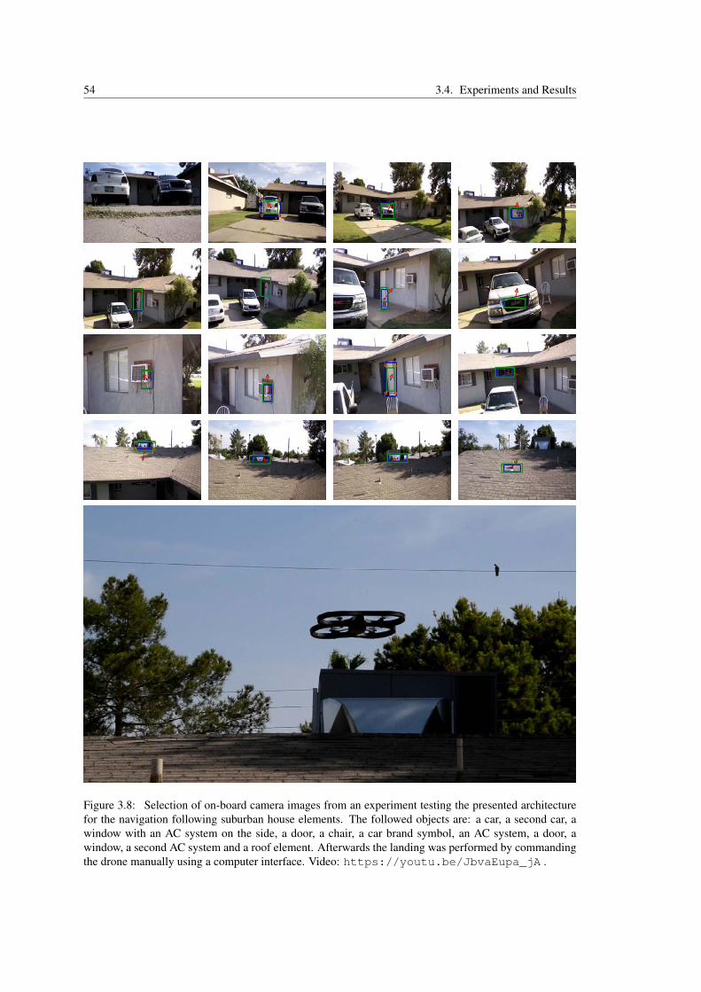
54 3.4. Experiments and Results
Figure 3.8: Selection of on-board camera images from an experiment testing the presented architecturefor the navigation following suburban house elements. The followed objects are: a car, a second car, awindow with an AC system on the side, a door, a chair, a car brand symbol, an AC system, a door, awindow, a second AC system and a roof element. Afterwards the landing was performed by commandingthe drone manually using a computer interface. Video: https://youtu.be/JbvaEupa_jA .
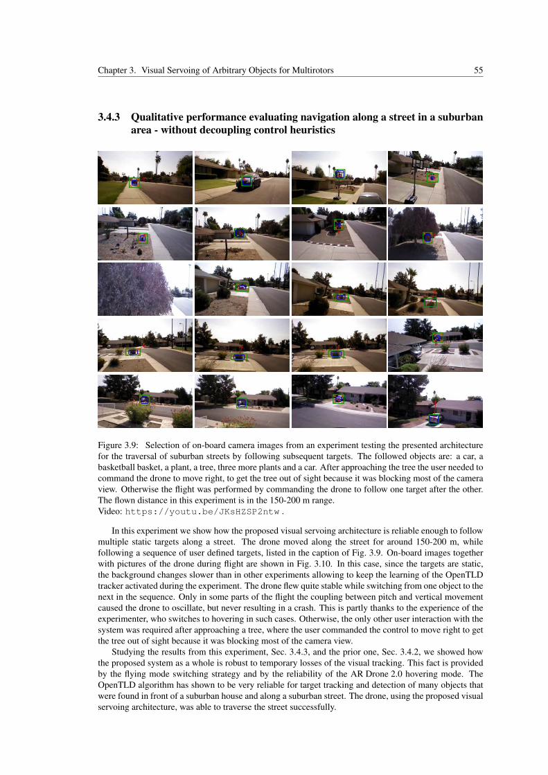
Chapter 3. Visual Servoing of Arbitrary Objects for Multirotors 55
3.4.3 Qualitative performance evaluating navigation along a street in a suburbanarea - without decoupling control heuristics
Figure 3.9: Selection of on-board camera images from an experiment testing the presented architecturefor the traversal of suburban streets by following subsequent targets. The followed objects are: a car, abasketball basket, a plant, a tree, three more plants and a car. After approaching the tree the user needed tocommand the drone to move right, to get the tree out of sight because it was blocking most of the cameraview. Otherwise the flight was performed by commanding the drone to follow one target after the other.The flown distance in this experiment is in the 150-200 m range.Video: https://youtu.be/JKsHZSP2ntw .
In this experiment we show how the proposed visual servoing architecture is reliable enough to followmultiple static targets along a street. The drone moved along the street for around 150-200 m, whilefollowing a sequence of user defined targets, listed in the caption of Fig. 3.9. On-board images togetherwith pictures of the drone during flight are shown in Fig. 3.10. In this case, since the targets are static,the background changes slower than in other experiments allowing to keep the learning of the OpenTLDtracker activated during the experiment. The drone flew quite stable while switching from one object to thenext in the sequence. Only in some parts of the flight the coupling between pitch and vertical movementcaused the drone to oscillate, but never resulting in a crash. This is partly thanks to the experience of theexperimenter, who switches to hovering in such cases. Otherwise, the only other user interaction with thesystem was required after approaching a tree, where the user commanded the control to move right to getthe tree out of sight because it was blocking most of the camera view.
Studying the results from this experiment, Sec. 3.4.3, and the prior one, Sec. 3.4.2, we showed howthe proposed system as a whole is robust to temporary losses of the visual tracking. This fact is providedby the flying mode switching strategy and by the reliability of the AR Drone 2.0 hovering mode. TheOpenTLD algorithm has shown to be very reliable for target tracking and detection of many objects thatwere found in front of a suburban house and along a suburban street. The drone, using the proposed visualservoing architecture, was able to traverse the street successfully.

56 3.4. Experiments and Results
Figure 3.10: Selection of on-board camera images from an experiment testing the presented architecturefor the traversal of suburban streets by following subsequent targets. (left) On-board image (right) Ap-proximately corresponding image of the drone during the flight experiment.Video: https://youtu.be/JKsHZSP2ntw .
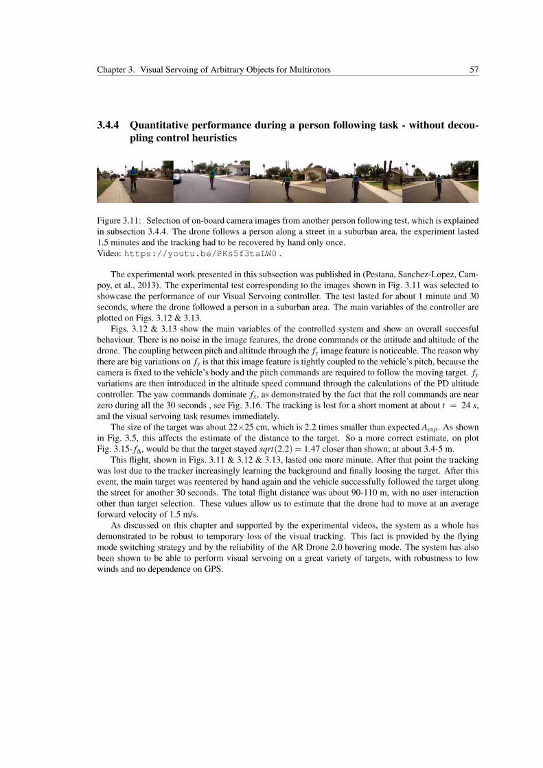
Chapter 3. Visual Servoing of Arbitrary Objects for Multirotors 57
3.4.4 Quantitative performance during a person following task - without decou-pling control heuristics
Figure 3.11: Selection of on-board camera images from another person following test, which is explainedin subsection 3.4.4. The drone follows a person along a street in a suburban area, the experiment lasted1.5 minutes and the tracking had to be recovered by hand only once.Video: https://youtu.be/PKs5f3taLW0 .
The experimental work presented in this subsection was published in (Pestana, Sanchez-Lopez, Cam-poy, et al., 2013). The experimental test corresponding to the images shown in Fig. 3.11 was selected toshowcase the performance of our Visual Servoing controller. The test lasted for about 1 minute and 30seconds, where the drone followed a person in a suburban area. The main variables of the controller areplotted on Figs. 3.12 & 3.13.
Figs. 3.12 & 3.13 show the main variables of the controlled system and show an overall succesfulbehaviour. There is no noise in the image features, the drone commands or the attitude and altitude of thedrone. The coupling between pitch and altitude through the fy image feature is noticeable. The reason whythere are big variations on fy is that this image feature is tightly coupled to the vehicle’s pitch, because thecamera is fixed to the vehicle’s body and the pitch commands are required to follow the moving target. fyvariations are then introduced in the altitude speed command through the calculations of the PD altitudecontroller. The yaw commands dominate fx, as demonstrated by the fact that the roll commands are nearzero during all the 30 seconds , see Fig. 3.16. The tracking is lost for a short moment at about t = 24 s,and the visual servoing task resumes immediately.
The size of the target was about 22×25 cm, which is 2.2 times smaller than expected Aexp. As shownin Fig. 3.5, this affects the estimate of the distance to the target. So a more correct estimate, on plotFig. 3.15- f∆, would be that the target stayed sqrt(2.2) = 1.47 closer than shown; at about 3.4-5 m.
This flight, shown in Figs. 3.11 & 3.12 & 3.13, lasted one more minute. After that point the trackingwas lost due to the tracker increasingly learning the background and finally loosing the target. After thisevent, the main target was reentered by hand again and the vehicle successfully followed the target alongthe street for another 30 seconds. The total flight distance was about 90-110 m, with no user interactionother than target selection. These values allow us to estimate that the drone had to move at an averageforward velocity of 1.5 m/s.
As discussed on this chapter and supported by the experimental videos, the system as a whole hasdemonstrated to be robust to temporary loss of the visual tracking. This fact is provided by the flyingmode switching strategy and by the reliability of the AR Drone 2.0 hovering mode. The system has alsobeen shown to be able to perform visual servoing on a great variety of targets, with robustness to lowwinds and no dependence on GPS.
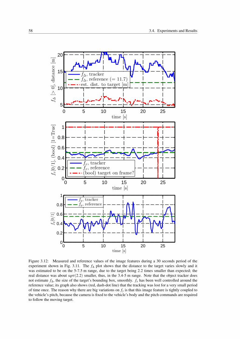
58 3.4. Experiments and Results
0 5 10 15 20 25
5
10
15
20f∆[>
0],distance
[m]
time [s]
f∆, trackerf∆, reference (= 11.7)est. dist. to target [m]
0 5 10 15 20 250
0.2
0.4
0.6
0.8
1
f x[0/1],(bool)[1=True]
time [s]
fx, trackerfx, reference(bool) target on frame?
0 5 10 15 20 250
0.2
0.4
0.6
0.8
1
f y[0/1]
time [s]
fy, trackerfy, reference
Figure 3.12: Measured and reference values of the image features during a 30 seconds period of theexperiment shown in Fig. 3.11. The f∆ plot shows that the distance to the target varies slowly and itwas estimated to be on the 5-7.5 m range, due to the target being 2.2 times smaller than expected; thereal distance was about sqrt(2.2) smaller, thus, in the 3.4-5 m range. Note that the object tracker doesnot estimate f∆, the size of the target’s bounding box, smoothly. fx has been well controlled around thereference value; its graph also shows (red, dash-dot line) that the tracking was lost for a very small periodof time once. The reason why there are big variations on fy is that this image feature is tightly coupled tothe vehicle’s pitch, because the camera is fixed to the vehicle’s body and the pitch commands are requiredto follow the moving target.

Chapter 3. Visual Servoing of Arbitrary Objects for Multirotors 59
0 5 10 15 20 25
−15
−10
−5
0
5
pitch,θ[deg]
time [s]
telemetrycontroller command
0 5 10 15 20 25
−4
−3
−2
−1
0
1
2
3
roll,φ[deg]
time [s]
telemetrycontroller command
0 5 10 15 20 25
0
0.5
1
1.5
2
Alt.[m
],Alt.speed[m
/s]
time [s]
Altitude, telemetryAlt. controller command
0 5 10 15 20 25
0
20
40
60
80
100
120
Yaw
,ψ
[deg]
dψ dtr[deg/s]
time [s]
yaw, telemetry (0 deg, North)yaw, controller command
Figure 3.13: Controller commands during a 30 seconds period of the experiment shown in Fig. 3.11. Asshown, none of the commands have a noticeable level of noise. The pitch command has a negative averagebecause the drone is following a person and it has to move forward. The roll command is approximatelyzero, as explained on the article the roll command is used just to stabilize the vehicle laterally. The dronestayed at an altitude of 1 to 2.0 m during the experiment, as measured by the ultrasound altitude sensor.The altitude speed command suffer from the influence of fy on the pitch commands, because fy is theimage feature used to feedback the altitude controller. The yaw plot shows a constant heading whilecrossing the street and then it changes when the drone moves parallel to the street.

60 3.4. Experiments and Results
3.4.5 Quantitative performance during a person following task - with decouplingcontrol heuristics
Figure 3.14: Selection of on-board camera images from another person following test, which is explainedin subsection 3.4.5. The robot tracks and follows a person along a street corridor in a suburban area. Theexperiment lasted 45 seconds where the AR Drone 2.0 covered a distance of about 120-140 m, thusnavigating at an average speed of 2.65-3.10 m/s. The orange arrow shows the decoupled altitude andlateral movement control actions. Video: https://youtu.be/67RXf5P7bfg .
The experimental work presented in this subsection was published in (Pestana, Sanchez-Lopez, Sari-palli, et al., 2014). The experimental test corresponding to the images shown in Fig. 3.14 was selectedto showcase the performance of our Visual Servoing controller. First, the tracker was trained to learn thetarget. Then, the learning feature of the tracker was switched off before the experimenter started running.The run lasted 45 seconds where the AR Drone 2.0 covered a distance of about 120-140 m. Thus, thedrone navigated at an average speed of 2.65-3.10 m/s. Thus far, these values show the peak performanceof our IBVS controller.
The Figs. 3.15 & 3.16 show the main variables of the controlled system during the experiment. Thereis low noise in the controlled image features, the drone commands and the attitude and altitude of thedrone. In spite of the decoupling heuristics, the coupling between pitch and altitude through the fv imagefeature near the end of the test is still noticeable. The reason why there are big variations in fv is that thisimage feature is tightly coupled to the vehicle’s pitch, because the camera is fixed to the vehicle’s bodyand the pitch commands are required to follow the moving target. fv variations are then introduced in thealtitude speed command through the calculations of the PD altitude controller. Another improvement thatwas introduced lately in our controller was the utilization of the outdoors hull and the yaw-lateral move-ment decoupling heuristic. Again, it is difficult to quantify the wind disturbance rejection improvementin any other way than investigating the external videos of the tests, which in our opinion show a clearimprovement.
As discussed in this chapter and supported by the experimental videos, the system as a whole hasdemonstrated to be robust to temporary loss of the visual tracking. This fact is provided by the flying modeswitching strategy and by the reliability of the AR Drone 2.0 hovering mode. The OpenTLD algorithm,to the extent of our limited group of experiments, has shown to be very reliable for target tracking anddetection and it has only rarely detected a wrong object.

Chapter 3. Visual Servoing of Arbitrary Objects for Multirotors 61
85 90 95 100 105 110 115 120 1250
10
20
30
40
f∆[>
0],distance
[m]
time [s]
f∆, trackerf∆, reference (= 11.7)est. dist. to target [m]
85 90 95 100 105 110 115 120 1250
0.2
0.4
0.6
0.8
1
f u[0/1],(bool)[1=True]
time [s]
fu, trackerfu, reference(bool) target on frame?
85 90 95 100 105 110 115 120 1250
0.2
0.4
0.6
0.8
1
f v[0/1]
time [s]
fv, trackerfv, reference
20 40 60 80 100 120
−30
−20
−10
0
10
20
YEast[m]
X North [m]
X Y , opt. flow EKF (·1.71)X Y , target position estimate
Figure 3.15: Measured and reference values of the image features during the experiment shown inFig. 3.14. The f∆ plot shows that the distance to the target varies slowly and it was estimated to be onthe 5-10.5 m range. Due to the target being 2.2 times smaller than expected; the real distance was aboutsqrt(2.2) smaller, thus, in the 3.5-7 m range. We note that the object tracker does not estimate f∆, the sizeof the target’s bounding box, smoothly all the time; the target bounding box sometimes jumps to anotherestimate on the image plane. fu has been well controlled around the reference value; it’s graph also shows(red, dash-dot line) that the tracking was not lost during this test. There are big variations in fv near theend of test which might be due to this feature being coupled to the vehicle’s pitch. The navigation speedof the vehicle or an estimation error on the vehicle’s pitch might be the cause of the decoupling’s heuristicdegradation on that part of the test. The last plot shows an estimate of the vehicle’s trajectory based on thevehicle’s telemetry using the EKF presented on (Pestana, 2012). The target’s position estimate is obtainedadding the estimate {∆xtme,∆ytme,∆ztme}, shown in Fig. 3.5, to the EKF’s drone’s position estimate.

62 3.4. Experiments and Results
85 90 95 100 105 110 115 120 125−15
−10
−5
0
5
pitch,θ[deg]
time [s]
telemetrycontroller command
85 90 95 100 105 110 115 120 125
−4
−2
0
2
roll,φ[deg]
time [s]
telemetrycontroller command
85 90 95 100 105 110 115 120 125
0
0.5
1
1.5
Alt.[m
],Alt.speed[m
/s]
time [s]
Altitude, telemetryAlt. controller command
85 90 95 100 105 110 115 120 125
−20
−10
0
10
20
30
40
Yaw
,ψ
[deg]
dψ dtr[deg/s]
time [s]
yaw, telemetryyaw, controller command
Figure 3.16: Controller commands during the experiment shown in Fig. 3.14. As shown, none of thecommands present a high level of noise. The pitch command has a negative average because the droneis following a person who is running and it has to move forward to keep up. The roll command is lowand only used during lateral movement or wind disturbance rejection to stabilize the vehicle’s lateralmovement. The drone stayed at an altitude of 1 to 1.5 m during most of the experiment, as measuredby the ultrasound altitude sensor. Near the end of the test, the altitude speed command is coupled withthe pitch command, which is caused by the coupling of the fv image feature with the pitch command.The yaw plot shows a constant heading during the first half of the experiment and then it shows the turnon the last part of the street corridor covered during the experiment, see the last plot of Fig. 3.15. Asexplained before, the yaw heading is controlled directly to keep the target in the middle of the imagewhich is important to avoid tracking loss events. The effect of the internal yaw reference ψtelemre f is thatthe vehicle tends to look at the target from the same direction.

Chapter 3. Visual Servoing of Arbitrary Objects for Multirotors 63
3.5 Future WorkThe first line is related with the tracking algorithm. Since the OpenTLD is one of the best tracking
algorithms which includes not only the tracking step, but also the detection one. However, it only providestranslation, and scaling to specify the real movement of the followed object in the image. But, thisassumption is restrictive. As future work, our aim is to use other trackers, like (Martínez et al., 2013),which provide the projective transformation in the image plane.
The second proposed improvement to the system is related with the reliability of the architecture.Now, when the tracked object leaves the image, the quadrotor starts to hover and it is not able to recoverit unless the object appears again in the image. One option could be to switch from the IBVS controllerto a PBVS controller when the object is lost. An EKF would be estimating the quadrotor’s and also thetarget’s 3D pose while the IBVS controller is working. Then when the target is lost, the PBVS controlleris enabled based on the EKF prediction of the followed object’s pose.
In the area of visual servoing there is an strong inter-dependence between the performance of thevisual tracker and the successful realization of an object following task by a controller. Therefore, newmethods could combine specific characteristics of the tracked objects and the surrounding environmentinto a better control strategy. For instance, it may be beneficial to select positions relative to the followedobject that result in viewing angles without light glare reflections or strong shadows. In the same direc-tion, the development of visual trackers that allow for object model introspection should be preferred. Forinstance, consider models that include the 3D structure of the object or the reflective properties of thedifferent surfaces of the object. A very interesting ongoing challenge that may require model introspec-tion is the International Aerial Robotics Competition (IARC) Mission 7, see Sec. I.4, where the droneneeds to physically interact with ground robots that exhibit pseudo-random navigation behavior. From anavigation stand point, obstacle avoidance needs to be incorporated more strongly into the visual servoingtask to enable following an object through a cluttered environment, like a sportsman through a forest.In this sense, obstacles that are difficult to map, such as trees, could be avoided considering their visualappearance rather than their difficult to reconstruct 3D structure.
3.6 ConclusionsIn this chapter, a novel visual based object tracking and following architecture for multirotor vehicles
is presented. The contributions of this work are two-fold:
• First, it has been demonstrated that current tracking algorithms, such as OpenTLD, can reliablywork on a fixed camera multirotor vehicle to feedback an Image Based Visual Servoing (IBVS)controller, even during high velocity autonomous navigation.
• Second, our architecture has been able to follow a large variety of unmarked targets of differentsizes and from a wide range of distances. Moreover, the algorithm is validated using a low-costplatform, the Parrot AR Drone 2.0, in outdoor conditions while tracking and following people. Thesystem has successfully and repeatedly handled occlusion events and tracked fast moving targets,such as a person running, showing the robustness of our system against wind disturbances andillumination changes.
The main features of our architecture that made it unique at the time of the publication of our worksare:
• Our system is able to follow and stabilize itself and it is able to track a large variety of differentobjects.
• Additionally, safety is assured even when the wireless connection is suddenly degraded, the trackingis lost or the target is occluded. This is achieved by using a multirotor platform that can attain on-board autonomous hovering by means of floor optical flow based odometry. The experimentalwork was performed using an AR Drone 2.0, and the algorithms where run on an off-board laptopcomputer via a WiFi link.
• Our system has been able to repeatedly perform object following tasks for long periods of timeof up to 7 minutes (see the related videos), and fully depleting the UAV battery, after the user isexperienced enough to understand the capabilities of our object following solution.

64 3.6. Conclusions
• Our system has been able to perform visual servoing with targets of varying size, from a quarter tomore than ten times the tunned target size, at varying distances from 1-2 m to 10-15 m of distancefrom the target, and it has has achieved person following at speeds up to 2.5-3.0 m/s for a period of45 seconds.
• The reliability of our system has been demonstrated in live demos: several performed by the CVG,at the SSRR2013 conference and with the ICG - TU Graz.
The main publications related to this chapter are:
• J. Pestana, J. L. Sanchez-Lopez, S. Saripalli, P. Campoy. “Computer Vision Based General ObjectFollowing for GPS-denied Multirotor Unmanned Vehicles”. In 2014 American Control Conference(ACC 2014). Portland, Oregon (United States). June 4th - 6th 2014
• J. Pestana, J. L. Sanchez-Lopez, S. Saripalli, P. Campoy. “Vision based GPS-denied Object track-ing and Following for Unmanned Aerial Vehicles”. Best Paper Award Finalist in 2013 The 11thIEEE International Symposium on Safety, Security, and Rescue Robotics (SSRR 2013). Linköping(Sweden). Oct 21-26, 2013.
The source of this aerial robotics visual servoing architecture has been released as open-source2, andit has been integrated by my colleagues as part of the stack for the control of multirotor MAVs from theCVAR/CVG (UPM) Aerostack3. The architecture has been successfully tested using an Asctec Pelicanand a powerful on-board computer, the Asctec Mastermind. Therefore, flights have been performed notrequiring an external ground station.
This aerial robotics visual servoing architecture has been showcased in several live demos:
• CivilDRON 2016 congress4, Madrid (Spain)Multi-robot mission and vision-based person followingMay 2016
• Semana de la Ciencia 2015 - Science Week 201556, Madrid (Spain)Multi-robot mission and vision-based person followingNovember 2-15, 2015
• 2015 European Robotics Week78, Madrid (Spain)Vision-based person followingSeptember 2015
• Noche Europea de los investigadores - European Researchers’ Night 20159
Multi-robot mission, vision-based person following and a simple search and rescue missionMadrid (Spain), September 2015
• 2014 European Robotics1011, Madrid (Spain)Vision-based person followingNovember 2014
• Semana de la Ciencia 2014 - Science Week 201412, Madrid (Spain)Multi-robot mission and vision-based person followingNovember 2014
2GitHub Repository: https://github.com/Vision4UAV/cvg_ardrone2_ibvs3GitHub Repository: https://github.com/Vision4UAV/Aerostack4CivilDRON 2016: http://www.aerpas.es/wp-content/uploads/2015/04/CivilDRON16_v2.pdf5Semana de la Ciencia 2015 - Website:http://bit.ly/2lN9RNg6Semana de la Ciencia 2015 - Results Report:http://bit.ly/2muELHG72015 European Robotics Week - Website: http://bit.ly/2mcMglt8European Robotics Week - Website: http://bit.ly/2mT12Bh9European Researchers’ Night 2015 - Website: http://bit.ly/2mM6a9Q
102014 European Robotics Week - Website: http://bit.ly/2mMaTIV11European Robotics Week - Website: http://bit.ly/2mT12Bh12Semana de la Ciencia 2014 - Results Report:http://bit.ly/2lNg1NA
Chapter 3. Visual Servoing of Arbitrary Objects for Multirotors 65
• OpenLabNight 201413, ICG - TU Graz (Austria)Vision-based person followingOctober 9, 2014
• Semana de la Ciencia 2013 - Science Week 201314, Madrid (Spain)Multi-robot mission and vision-based person followingNovember 4-17, 2013
• The 11th IEEE International Symposium on Safety, Security, and Rescue Robotics (SSRR 2013)15
Vision-based person followingLinköping (Sweden), October 21-26, 2013
For a full list of videos showing the performance of the presented visual servoing architecture thereader is referred to Sec. 3.4.1.
13OpenLabNight 2014, ICG - TU Graz, Website: http://bit.ly/2mwigU414Semana de la Ciencia 2013 - Results Report:http://bit.ly/2npz2lF15SSRR 2013 Demos Website:http://www.ssrr-conference.org/2013/Demos.html

66 3.7. Chapter Bibliography
3.7 Chapter BibliographyAchtelik, M., Achtelik, M., Weiss, S., and Siegwart, R. (2011). “Onboard IMU and monocular vision
based control for MAVs in unknown in- and outdoor environments”. In: Robotics and Automation(ICRA), 2011 IEEE International Conference on, pp. 3056–3063 (cit. on p. 45).
Mani Monajjemi (2012). ardrone_autonomy : A ROS Driver for ARDrone 1.0 & 2.0. https : / /github.com/AutonomyLab/ardrone_autonomy. Autonomy Lab, Simon Fraser Univer-sity (cit. on p. 46).
Argyros, A., Georgiadis, P., Trahanias, P., and Tsakiris, D. (2002). “Semi-autonomous Navigation of aRobotic Wheelchair”. Journal of Intelligent and Robotic Systems 34 (3), pp. 315–329 (cit. on p. 45).
Babenko, B., Yang, M.-H., and Belongie, S. (2009). “Visual tracking with online Multiple Instance Learn-ing”. In: Computer Vision and Pattern Recognition, 2009. CVPR 2009. IEEE Conference on, pp. 983–990 (cit. on p. 45).
Bills, C., Chen, J., and Saxena, A. (2011). “Autonomous MAV flight in indoor environments using singleimage perspective cues”. In: Robotics and Automation (ICRA), 2011 IEEE International Conferenceon, pp. 5776–5783 (cit. on pp. 43, 45).
Bourquardez, O., Mahony, R., Guenard, N., Chaumette, F., Hamel, T., and Eck, L. (2009). “Image-BasedVisual Servo Control of the Translation Kinematics of a Quadrotor Aerial Vehicle”. Robotics, IEEETransactions on 25.3, pp. 743–749 (cit. on p. 45).
Chaumette, F. (1998). “Potential problems of stability and convergence in image-based and position-basedvisual servoing”. In: The confluence of vision and control. Springer, pp. 66–78 (cit. on p. 44).
Chesi, G. (2009). “Visual servoing path planning via homogeneous forms and LMI optimizations”.Robotics, IEEE Transactions on 25.2, pp. 281–291 (cit. on p. 45).
Chesi, G. and Vicino, A. (2004). “Visual servoing for large camera displacements”. Robotics, IEEE Trans-actions on 20.4, pp. 724–735 (cit. on p. 45).
Comport, A., Mahony, R., and Spindler, F. (2011). “A visual servoing model for generalised cameras: Casestudy of non-overlapping cameras”. In: Robotics and Automation (ICRA), 2011 IEEE InternationalConference on, pp. 5683–5688 (cit. on p. 45).
Corke, P. I. et al. (1996). Visual Control of Robots: high-performance visual servoing. Research StudiesPress Taunton, UK (cit. on p. 44).
Danelljan, M., Khan, F. S., Felsberg, M., Granström, K., Heintz, F., Rudol, P., Wzorek, M., Kvarnström,J., and Doherty, P. (2014). “A low-level active vision framework for collaborative unmanned aircraftsystems”. In: Workshop at the European Conference on Computer Vision. Springer, pp. 223–237 (cit.on p. 45).
Danelljan, M., Shahbaz Khan, F., Felsberg, M., and Van de Weijer, J. (2014). “Adaptive color attributes forreal-time visual tracking”. In: Proceedings of the IEEE Conference on Computer Vision and PatternRecognition, pp. 1090–1097 (cit. on p. 45).
Deng, H., Zhao, X., and How, Z. (2009). “A Vision-Based Ground Target Tracking System for a Small-Scale Autonomous Helicopter”. Image and Graphics, International Conference on, pp. 739–743 (cit.on p. 45).
Engel, J., Sturm, J., and Cremers, D. (2012). “Camera-Based Navigation of a Low-Cost Quadrocopter”.In: Proc. of the International Conference on Intelligent Robot Systems (IROS) (cit. on pp. 43, 45).
Espiau, B., Chaumette, F., and Rives, P. (1992). “A new approach to visual servoing in robotics”. ieeeTransactions on Robotics and Automation 8.3, pp. 313–326 (cit. on p. 45).
Fahd Rafi Saad Khan, K. S. and Shah, M. (2006). “Autonomous target following by unmanned aerialvehicles”. In: Proc. SPIE. Orlando (Kissimmee), FL, USA (cit. on p. 45).
Feddema, J. T. and Mitchell, O. R. (1989). “Vision-guided servoing with feature-based trajectory genera-tion [for robots]”. Robotics and Automation, IEEE Transactions on 5.5, pp. 691–700 (cit. on p. 44).
Fomena, R. T. and Chaumette, F. (2007). “Visual servoing from spheres using a spherical projectionmodel”. In: Robotics and Automation, 2007 IEEE International Conference on. IEEE, pp. 2080–2085(cit. on p. 44).
Haag, K., Dotenco, S., and Gallwitz, F. (2015). “Correlation filter based visual trackers for person pursuitusing a low-cost Quadrotor”. In: Innovations for Community Services (I4CS), 2015 15th InternationalConference on. IEEE, pp. 1–8 (cit. on p. 45).

Chapter 3. Visual Servoing of Arbitrary Objects for Multirotors 67
Hamel, T. and Mahony, R. (2002a). “Visual servoing of an under-actuated dynamic rigid-body system: animage-based approach”. Robotics and Automation, IEEE Transactions on 18.2, pp. 187–198 (cit. onp. 44).
Hamel, T. and Mahony, R. (2002b). “Visual servoing of an under-actuated dynamic rigid-body system: animage-based approach”. Robotics and Automation, IEEE Transactions on 18.2, pp. 187–198 (cit. onp. 44).
Hutchinson, S and Chaumette, F (2006). “Visual servo control, Part I: Basic approaches”. IEEE Roboticsand Automation Magazine 13.4, pp. 82–90 (cit. on p. 44).
Hutchinson, S and Chaumette, F (2007). “Visual servo control, Part II: Advanced approaches”. IEEERobotics and Automation Magazine 14.1, pp. 109–118 (cit. on p. 44).
Kalal, Z. (2011). “Tracking Learning Detection”. PhD thesis. University of Surrey (cit. on pp. 43, 45, 46).Kalal, Z., Mikolajczyk, K., and Matas, J. (2012). “Tracking-Learning-Detection”. IEEE Transactions on
Pattern Analysis and Machine Intelligence 34.7, pp. 1409–1422 (cit. on pp. 43, 45, 46).Korodi, A., Codrean, A., Banita, L., and Volosencu, C. (2008). “Aspects regarding the object following
control procedure for wheeled mobile robots”. WSEAS Trans. Sys. Ctrl. 3 (6), pp. 537–546 (cit. onp. 45).
Lapresté, J.-T. and Mezouar, Y. (2004). “A Hessian approach to visual servoing”. In: Intelligent Robotsand Systems, 2004.(IROS 2004). Proceedings. 2004 IEEE/RSJ International Conference on. Vol. 1.IEEE, pp. 998–1003 (cit. on p. 45).
Lin, F., Chen, B., Lum, K. Y., and Lee, T. (2010). “A robust vision system on an unmanned helicopterfor ground target seeking and following”. In: Intelligent Control and Automation (WCICA), 2010 8thWorld Congress on, pp. 276–281 (cit. on p. 45).
Mahony, R., Corke, P., and Chaumette, F. (2002). “Choice of image features for depth-axis control inimage based visual servo control”. In: Intelligent Robots and Systems, 2002. IEEE/RSJ InternationalConference on. Vol. 1, 390–395 vol.1 (cit. on p. 44).
Mahony, R., Brasch, A., Corke, P., and Hamel, T. (2005). “Adaptive depth estimation in image basedvisual servo control of dynamic systems.” In: Decision and Control, 2005 and 2005 European ControlConference. CDC-ECC ’05. 44th IEEE Conference on, pp. 5372–5378 (cit. on p. 45).
Mahony, R., Corke, P., and Chaumette, F. (2002). “Choice of image features for depth-axis control inimage based visual servo control”. In: Intelligent Robots and Systems, 2002. IEEE/RSJ InternationalConference on. Vol. 1. IEEE, pp. 390–395 (cit. on p. 44).
Malis, E. (2004). “Improving vision-based control using efficient second-order minimization techniques”.In: Robotics and Automation, 2004. Proceedings. ICRA’04. 2004 IEEE International Conference on.Vol. 2. IEEE, pp. 1843–1848 (cit. on p. 45).
Martínez, C., Mondragón, I. F., Campoy, P., Sánchez-López, J. L., and Olivares-Méndez, M. A. (2013). “AHierarchical Tracking Strategy for Vision-Based Applications On-Board UAVs”. Journal of Intelligent& Robotic Systems, pp. 1–23 (cit. on pp. 45, 63).
Mezouar, Y. and Chaumette, F. (2002). “Path planning for robust image-based control”. Robotics andAutomation, IEEE Transactions On 18.4, pp. 534–549 (cit. on p. 45).
Mondragoón, I., Campoy, P., Olivares-Mendez, M., and Martinez, C. (2011). “3D object following basedon visual information for Unmanned Aerial Vehicles”. In: Robotics Symposium, 2011 IEEE IX LatinAmerican and IEEE Colombian Conference on Automatic Control and Industry Applications (LARC),pp. 1–7 (cit. on pp. 43, 45).
Nebehay, G. (2012). “Robust Object Tracking Based on Tracking-Learning-Detection”. MA thesis. Aus-tria: Vienna University of Technology (cit. on p. 46).
Kalal, Z (2011). OpenTLD object image tracker source repositories: (2011) Kalal, Z (PhD Thesis); Mat-lab OpenTLD implementation https://github.com/zk00006/OpenTLD (cit. on p. 46).
Nebehay, G (2012). OpenTLD object image tracker source repositories: (2012) Nebehay, G (Msc. Thesis);C++ OpenTLD implementation https://github.com/gnebehay/OpenTLD (cit. on p. 46).
Chauvin, R (2012). OpenTLD object image tracker source repositories: (2013) Chauvin, R; C++ ROSOpenTLD wrapper https://github.com/Ronan0912/ros_opentld (cit. on p. 46).
Pestana, J. (2012). “On-board control algorithms for Quadrotors and indoors navigation”. MA thesis.Spain: Universidad Politécnica de Madrid (cit. on pp. 49, 61).
Pestana, J., Mellado-Bataller, I., Fu, C., Sanchez-Lopez, J. L., Mondragon, I. F., and Campoy, P. (2013).“A general purpose configurable navigation controller for micro aerial multirotor vehicles”. In: Un-
68 3.7. Chapter Bibliography
manned Aircraft Systems (ICUAS), 2013 International Conference on. IEEE, pp. 557–564 (cit. onp. 49).
Pestana, J., Sanchez-Lopez, J. L., Campoy, P., and Saripalli, S. (2013). “Vision based gps-denied objecttracking and following for unmanned aerial vehicles”. In: 2013 IEEE International Symposium onSafety, Security, and Rescue Robotics (SSRR). IEEE, pp. 1–6 (cit. on p. 57).
Pestana, J., Sanchez-Lopez, J. L., Saripalli, S., and Campoy, P. (2014). “Computer vision based generalobject following for GPS-denied multirotor unmanned vehicles”. In: 2014 American Control Confer-ence. IEEE, pp. 1886–1891 (cit. on p. 60).
Quigley, M., Gerkey, B., Conley, K., Faust, J., Foote, T., Leibs, J., Berger, E., Wheeler, R., and Ng,A. (2009). “ROS : an open-source Robot Operating System”. In: IEEE International Conference onRobotics and Automation (ICRA 2009) (cit. on p. 46).
Rives, P. and Azinheira, J. R. (2004). “Linear structures following by an airship using vanishing point andhorizon line in a visual servoing scheme”. In: Robotics and Automation, 2004. Proceedings. ICRA’04.2004 IEEE International Conference on. Vol. 1. IEEE, pp. 255–260 (cit. on p. 45).
Ross, S., Melik-Barkhudarov, N., Shankar, K. S., Wendel, A., Dey, D., Bagnell, J. A., and Hebert, M.(2013). “Learning monocular reactive uav control in cluttered natural environments”. In: Robotics andAutomation (ICRA), 2013 IEEE International Conference on. IEEE, pp. 1765–1772 (cit. on pp. 43,45).
Saripalli, S. and Sukhatme, G. S. (2007). “Landing a Helicopter on a Moving Target”. In: Proceedingsof IEEE International Conference on Robotics and Automation. Rome, Italy, pp. 2030–2035 (cit. onp. 45).
Savkin, A. and Teimoori, H. (2008). “Bearings-only guidance of an autonomous vehicle following amoving target with a smaller minimum turning radius”. In: Decision and Control, 2008. CDC 2008.47th IEEE Conference on, pp. 4239–4243 (cit. on p. 45).
Schramm, F., Geffard, F., Morel, G., and Micaelli, A. (2007). “Calibration free image point path planningsimultaneously ensuring visibility and controlling camera path”. In: Robotics and Automation, 2007IEEE International Conference on. IEEE, pp. 2074–2079 (cit. on p. 45).
Tahri, O. and Chaumette, F. (2005a). “Point-based and region-based image moments for visual servoingof planar objects”. Robotics, IEEE Transactions on 21.6, pp. 1116–1127 (cit. on p. 44).
Tahri, O., Mezouar, Y., Chaumette, F., and Corke, P. (2010). “Decoupled Image-Based Visual Servoing forCameras Obeying the Unified Projection Model”. Robotics, IEEE Transactions on 26.4, pp. 684–697(cit. on pp. 44, 47).
Tahri, O. (2004). “Utilisation des moments en asservissement visuel et en calcul de pose”. PhD thesis.Rennes 1 (cit. on p. 44).
Tahri, O. and Chaumette, F. (2005b). “Point-based and region-based image moments for visual servoingof planar objects”. Robotics, IEEE Transactions on 21.6, pp. 1116–1127 (cit. on p. 44).
Tahri, O., Chaumette, F., and Mezouar, Y. (2008). “New decoupled visual servoing scheme based oninvariants from projection onto a sphere”. In: Robotics and Automation, 2008. ICRA 2008. IEEEInternational Conference on. IEEE, pp. 3238–3243 (cit. on p. 45).
Tahri, O. and Mezouar, Y. (2010). “On visual servoing based on efficient second order minimization”.Robotics and Autonomous Systems 58.5, pp. 712–719 (cit. on p. 45).
Tahri, O., Mezouar, Y., Chaumette, F., and Corke, P. (2009). “Generic decoupled image-based visualservoing for cameras obeying the unified projection model”. In: Robotics and Automation, 2009.ICRA’09. IEEE International Conference on. IEEE, pp. 1116–1121 (cit. on p. 45).
Teuliere, C., Eck, L., and Marchand, E. (2011). “Chasing a moving target from a flying UAV”. In: 2011IEEE/RSJ International Conference on Intelligent Robots and Systems. IEEE, pp. 4929–4934 (cit. onp. 45).
Zhang, H. and Ostrowski, J. (1999). “Visual servoing with dynamics: control of an unmanned blimp”. In:Robotics and Automation, 1999. Proceedings. 1999 IEEE International Conference on. Vol. 1, 618–623 vol.1 (cit. on p. 45).

Chapter 4Smooth Trajectory Planning forMultirotors
4.1 IntroductionThis chapter describes the development of a trajectory planner that generates smooth sampled
obstacle-free trajectories and accompanying speed and acceleration plans for multirotors. This trajectoryplanner was developed to participate in the Simulation Contest of the European Robotics Challenge (Eu-RoC 2014) - Challenge 3, which focus was on drones applied to plant servicing and inspection. Theplanner was later improved, verified experimentally and executed on-board a quadrotor while participat-ing in the 2016 DJI Developer Challenge. The main purpose of this module is to generate paths that canbe traversed smoothly and fast by the quadrotor, while remaining at a safe distance from nearby obstacles.
A state-of-the-art planner is used to obtain a path that minimizes a weighted length. Each stretch ofpath is weighted depending on various factors, e. g. proximity to obstacles. A fixed amount of time isalotted for this task, and the best solution found so far is used for the rest of the calculations. With theseobjectives in mind:
• The planner calculates obstacle-free trajectories for multirotor drones. Given that these platformsare omnidirectional, they can move at any point in any direction, the trajectory planning step isperformed in 3D space; no attitude angles, only position.
• A map of the environment must be provided as an octomap representation. The map does not needto be static, this planner was extended to work in dynamic maps/environments while participatingin the 2016 DJI Developer Challenge.
• The generated paths stay away from obstacles by associating, inside an optimization formulation,an increased cost to navigating near them. Similarly a higher cost is associated to trajectories thatrealize unnecessary changes in altitude.
• The trajectories are smoothed in order to avoid sharp angles in curves, so that the multirotor canfollow them smoothly without decelerating strongly on every curve. The smoothing operation is
69

70 4.2. State of the Art
obstacle-aware, which ensures that the smoothed trajectory is approximately as far from obstaclesas the originally planned raw trajectory.
• The trajectories are finely sampled to allow for the estimation of the radius of curvature at everywaypoint of the trajectory. Its calculation is required to compute a time of passage through everywaypoint, a speed and an acceleration plan.
• In addition to the positions, the sets of values for the time of passage, speed and acceleration areused by a controller to calculate interpolating splines of third order (or higher, depending on theutilized data) over the waypoints of the path. The resulting spline is later used during trajectoryexecution by the controller to perform navigation.
• For our work, it is important to use algorithms that can provide a feasible trajectory in a reasonableamount of time, for path lengths of 30-150 m, so that they can be used in real-time operation in theon-board computer of the multirotor. Consider as an application scenario the plant servicing andinspection in industrial environments.
The layout of this chapter is the following. First, the state of the art and a summary of the devel-oped trajectory planning approach is presented. Then, the theoretical background related to the developedtrajectory planner is introduced. It includes a description of the probabilistic map representation Oc-tomap (Hornung et al., 2013), an efficient calculation of the distance to obstacles (Lau et al., 2013) usingthe said map representation, the two tested state-of-the-art trajectory planning algorithms ProbabilisticRoadMap Star (PRM∗) (Karaman et al., 2011; Kavraki et al., 1996) and Rapidly-exploring Random TreeStar (RRT∗) (LaValle, 1998); and the open-source libraries utilized during implementation (Sucan et al.,2012). Then, the detailed description of the developed planner is introduced; including the related uti-lization of the said open-source libraries. Afterwards, the results in two international competitions arediscussed, including a description of the utilized experimental platform. The chapter finishes with theconclusions and the objectives achieved along with the utilization of the developed trajectory planner.
4.2 State of the ArtModern efficient trajectory planning approaches for multirotors are based on them being differentially
flat dynamic systems. For instance, the control law by Fritsch et al. (Fritsch et al., 2012) can be consid-ered to be built on the differential flatness property of the dynamics of the multirotor (Fliess et al., 1995;Murray et al., 1995), which is well explained in (Mellinger et al., 2011). A system is differentially flat ifthere exists a set of outputs from it which fully determine the state of the system given the values of theflat outputs and their derivatives (to a given order). When a non-linear system is differentially flat, thischaracteristic can be used for both: control and trajectory generation (Dunbar et al., 2003; Van Nieuw-stadt et al., 1998). Some of the first works to exploit the differential flatness of multirotors to performtrajectory planning and generation was performed by (Cowling et al., 2010). In this work, many differentapproaches to parametrize the trajectory were proposed: Chebyshev polynomials, Laguerre polynomials,trigonometric functions and piecewise polynomials among others; however results were only shown for asingle polynomial per coordinate.
Probably, one of the most known works that makes use of the differential flatness to perform trajectorygeneration and tracking with quadrotors was carried out by Daniel Mellinger et al. (Mellinger et al., 2011)from the GRASP Laboratory. In this work the trajectory was divided in segments were a high-degreepolynomial is fit, and the polynomials were fitted optimizing a Quadratic Programming (QP) problemthat minimize the snap of the trajectory and includes corridor constraints, that allow to traverse tightpassages demonstrated by making the quadrotor go through static and moving hula hoops. In this work,the trajectory could also be scaled in time to perform either faster tracking or a slower more stable flight.
However, it was not yet clearly developed how this trajectory generation methods can be combinedwith traditional trajectory planning techniques, such as Probabilistic RoadMaps (PRMs) or Rapidly ex-ploring Random Tree (RRTs). The work by Charles Richter et al. (Richter, Charles et al., 2013; Richteret al., 2013) from the MIT, showed how to input a trajectory calculated by an RRT* planning algorithminto a Quadratic Programming (QP) to calculate an optimal flight trajectory using splines. Their novelapproach optimizes the trajectory in terms of traversal time and aggressiveness, so that it can be used to
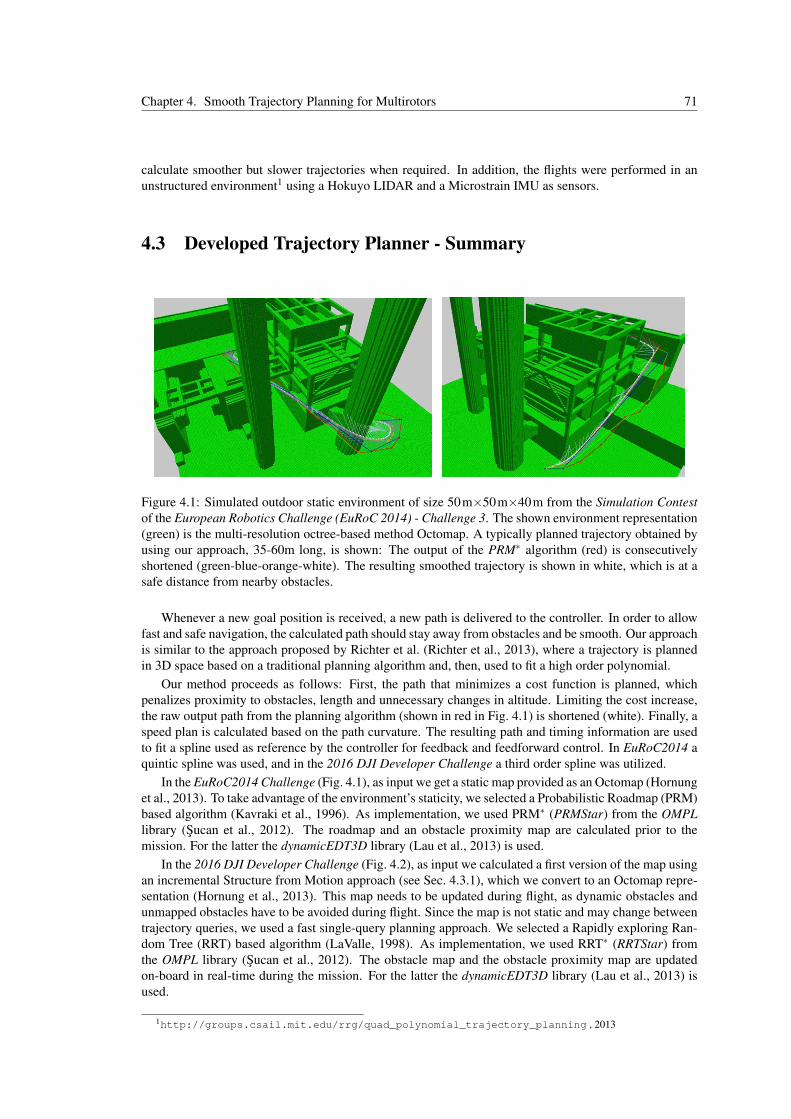
Chapter 4. Smooth Trajectory Planning for Multirotors 71
calculate smoother but slower trajectories when required. In addition, the flights were performed in anunstructured environment1 using a Hokuyo LIDAR and a Microstrain IMU as sensors.
4.3 Developed Trajectory Planner - Summary
Figure 4.1: Simulated outdoor static environment of size 50m×50m×40m from the Simulation Contestof the European Robotics Challenge (EuRoC 2014) - Challenge 3. The shown environment representation(green) is the multi-resolution octree-based method Octomap. A typically planned trajectory obtained byusing our approach, 35-60m long, is shown: The output of the PRM∗ algorithm (red) is consecutivelyshortened (green-blue-orange-white). The resulting smoothed trajectory is shown in white, which is at asafe distance from nearby obstacles.
Whenever a new goal position is received, a new path is delivered to the controller. In order to allowfast and safe navigation, the calculated path should stay away from obstacles and be smooth. Our approachis similar to the approach proposed by Richter et al. (Richter et al., 2013), where a trajectory is plannedin 3D space based on a traditional planning algorithm and, then, used to fit a high order polynomial.
Our method proceeds as follows: First, the path that minimizes a cost function is planned, whichpenalizes proximity to obstacles, length and unnecessary changes in altitude. Limiting the cost increase,the raw output path from the planning algorithm (shown in red in Fig. 4.1) is shortened (white). Finally, aspeed plan is calculated based on the path curvature. The resulting path and timing information are usedto fit a spline used as reference by the controller for feedback and feedforward control. In EuRoC2014 aquintic spline was used, and in the 2016 DJI Developer Challenge a third order spline was utilized.
In the EuRoC2014 Challenge (Fig. 4.1), as input we get a static map provided as an Octomap (Hornunget al., 2013). To take advantage of the environment’s staticity, we selected a Probabilistic Roadmap (PRM)based algorithm (Kavraki et al., 1996). As implementation, we used PRM∗ (PRMStar) from the OMPLlibrary (Sucan et al., 2012). The roadmap and an obstacle proximity map are calculated prior to themission. For the latter the dynamicEDT3D library (Lau et al., 2013) is used.
In the 2016 DJI Developer Challenge (Fig. 4.2), as input we calculated a first version of the map usingan incremental Structure from Motion approach (see Sec. 4.3.1), which we convert to an Octomap repre-sentation (Hornung et al., 2013). This map needs to be updated during flight, as dynamic obstacles andunmapped obstacles have to be avoided during flight. Since the map is not static and may change betweentrajectory queries, we used a fast single-query planning approach. We selected a Rapidly exploring Ran-dom Tree (RRT) based algorithm (LaValle, 1998). As implementation, we used RRT∗ (RRTStar) fromthe OMPL library (Sucan et al., 2012). The obstacle map and the obstacle proximity map are updatedon-board in real-time during the mission. For the latter the dynamicEDT3D library (Lau et al., 2013) isused.
1http://groups.csail.mit.edu/rrg/quad_polynomial_trajectory_planning , 2013

72 4.3. Developed Trajectory Planner - Summary
Figure 4.2: Outdoor map environment of size 55m×170m×40m generated using the “Off-board Ap-proach” explained in Sec. 4.3.1. The shown environment representation is the Octomap obstacle map.Typical planned trajectories, up to around 100m long, are shown: The output of the RRT∗ algo-rithm (red) is consecutively shortened (green-blue-orange-white). The resulting smoothed trajectoryis shown in white, which is at a safe distance from nearby obstacles. Our DJI M100 quadrotor flewsuch trajectories as part of our second deliverable for the 2016 DJI Developer Challenge, see video:http://bit.ly/2faublQ.
4.3.1 Online Structure-from-Motion (SfM) - Rescue Area Real-Time Mapping -2016 DJI Developer Challenge
We use an in-house 3D Reconstruction and Structure from Motion library developed over the years bythe Institute of Computer Graphics of the TU Graz2. We use the real-time (on-line) Structure-from-Motion(SfM) pipeline which was first proposed and developed by Hoppe et al. (Hoppe, Klopschitz, Rumpler, etal., 2012). This Online SfM framework (or pipeline) is very runtime efficient. It uses SIFT features (Lowe,2004). The model is initialized from the first two images for which a valid relative pose estimate can becomputed. It iteratively utilizes the fast absolute pose estimation developed by Kneip et al. (Kneip et al.,2011) to align the latest acquired high-resolution image to the current sparse 3D model in real-time. Usingan incremental and real-time version of Line3D++ (Hofer et al., 2016), a set of 3D lines is also calculatedfrom the aligned images. Thus, the model consists of a sparse point cloud, a set of line segments and thecamera poses related to each acquired image. The set of 3D lines helps to visually interpret the sparse 3Dmap, specially in the case of man-made environments (and other line-rich environments).
Utilizing the GPS measurements at the acquisition time of the images, the sparse 3D map is correctly
2http://icg.tugraz.at/

Chapter 4. Smooth Trajectory Planning for Multirotors 73
Figure 4.3: Outdoor map environment of size 60m×95m generated using the “Real-Time On-boardApproach” explained in Sec. 4.3.1. The left image is an overview of the mapped area, the target 50m×50m region is around the parking lot. Man-made obstacles, such as the buildings and cars, and big treesare quite well acquired as obstacles. However, smaller tries are often not correctly mapped and need tobe sensed during nearby flight at low altitude. Our DJI M100 quadrotor is equipped with several stereoheads (the DJI Guidance System) that correctly acquires point-clouds of trees; which we use to update themap with dynamic and unmapped obstacles during flight. The trajectory planner, then, uses the updatedmap to calculate obstacle free smooth paths in the area.
scaled and geo-referenced. The on-board implementation matches the GPS measurements to the cameralocations of the model by means of a robust RANSAC-based minimum least squares minimization of thedistance between both sets of locations. This effectively provides the correct scale, rotation and relativetranslation for the sparse 3D map. In addition, a better geo-referenciation can be obtained by placinggeo-referenced fiducial markers on site (Rumpler et al., 2016), but this approach was not possible in theSearch and Rescue scenario proposed in the 2016 DJI Developer Challenge.
In addition to the sparse 3D map, the pipeline also creates a surface model on-the-fly (Hoppe, Klops-chitz, Donoser, et al., 2013). The current implementation uses the approach by Labatut et al. (Labatut etal., 2007), rather than the approach outlined in Hoppe’s work (Hoppe, Klopschitz, Donoser, et al., 2013).This model can then directly be converted to an Octomap (Hornung et al., 2013) by direct point-samplingof the triangle-mesh. The obtained Octomap can be updated in real-time and utilized by the presentedtrajectory planner during flight.
All these map representations of the environment are geo-referenced, based on the GPS data fromthe acquired images. This allows to locate the drone, a DJI M100 quadrotor, with respect to this mapby simply using its GPS measurements. Other advantages of the geo-referencing of the map are that:no-fly zones can be added, and that the survivors can be located on the acquired map and referred tocorresponding images (and pixel locations) of the mapping dataset.
To generate the map, the multirotor is first flown autonomously over the area to be mapped at a safealtitude (e. g. 34m). A set of top down images is used to generate a sparse 3D map on-the-fly, as explainedabove. Simultaneously a 3D mesh is fitted to the sparse model, which is finally used to obtain the Octomaprepresentation of the environment, the obstacle map, by fine sampling of the said 3D mesh.
[Off-board Approach] During our first experiments, the Online SfM framework was used to processan image stream acquired by flying above the Rescue Area from a safe height. The images from theZenmuse X3 Gimbal (resolution of 1280x720 pixels) were processed on a laptop during the acquisitionflight. Our Online SfM runs faster than real-time on a 4 fps image stream.
[Real-Time On-board Approach] Currently the image stream from the Zenmuse X3 Gimbal (reso-lution of 1280x720 pixels) is fully processed on-board our DJI M100 quadrotor. This is made possibleby leveraging the GPU of the on-board computer, the DJI Manifold (basically a Nvidia Tegra K1 de-velopment board). The Online SfM pipeline is able to process 1 image every 3.0s during flight (or 1image every 1.5s at the office). An area of 50×50m with a final map size of up to around 65×105m(for level-ground) is mapped on-board the DJI M100 in 2.5min. This time includes the overview-flight,acquisition of images, the generation of the sparse 3D model, the meshing, the geo-referenciation anthe conversion to the Octomap obstacle map representation. One of the seven 3D reconstructions (Oc-
74 4.4. Trajectory Planning - Theoretical Background
tomap model), processed on-board during the 2016 DJI Developer Challenge is shown in the see video:http://bit.ly/2faublQ, and another map obtained in the same fashion is shown in Fig. 4.3.
4.4 Trajectory Planning - Theoretical BackgroundFor a comprehensive description of trajectory planning algorithms, the reader is referred to the freely
available book from S.M. LaValle (LaValle and Kuffner, 2001). In the context of this chapter, the objectiveof the trajectory planning task is to calculate a smooth path to the next target point from the currentposition of the multirotor, while remaining reasonably away from obstacles and resulting in a reasonablyshort path. Staying away from obstacles and calculating the shortest path are often rather opposite andcompeting objectives that need to be combined in a common weighting scheme. The path that achievesboth objectives “reasonably” is preferred over the shortest path or over the one that stays away fromobstacles as much as possible.
The reason why the planning problem is focused on the positions only is the following. Commonmultirotors can theoretically follow trajectories defined in position as long as they are continuous upto the fourth derivative, with the heading angle being continuous up to the second derivative (Fritschet al., 2012; Mellinger et al., 2011). The heading can otherwise be set to look in any desired directionduring the trajectory. This very interesting property of the quadrotor dynamics model is exploited in theworks by Mellinger et al. (Mellinger et al., 2011) and Fritsch et al. (Fritsch et al., 2012); and it can beunderstood as the quadrotor dynamics model being differentially flat with respect to the trajectory pathand heading. This property allows to solve the trajectory planning problem including the dynamics of thequadrotor intrinsically considering a position-only path, by just enforcing the continuity of the path up tothe said derivatives. This is a very advantageous approach, because it allows to use simpler path planningalgorithms with a faster computation time than general-purpose dynamics-aware trajectory planners.
A map representation is needed to describe the environment and divide it between the free-space andthe obstacle-space. For a given robot, this allows to determine which positions of the vehicle do not col-lide with obstacles and are thus permissible. In order to achieve real-time execution time, an efficient maprepresentation able to represent general-shaped obstacles is used, the Octomap map representation (Hor-nung et al., 2013). This map representation has the additional advantage to be able to encode mappinguncertainty, by encoding the probability of a point in space to be occupied by an obstacle. A relatedopen-source algorithm specifically designed for regular grid-based representations of 3D space, includingOctomap, is available to efficiently determine the distance of every point in the free-space to the closestobstacle (Lau et al., 2013).
In order to achieve a real-time competitive execution time while calculating an optimal path, sampling-based trajectory planning algorithms were selected. The reason for selecting sampling-based methods isthat they have proofed to work very well in practice. More specific reasons for this decision are:
• the speed with which the solution is obtained will not depend on the sampling resolution of theOctomap (as it would happen with a grid-based planning approach).
• that the planning time should scale better with the complexity and the size of the map than grid-based approaches.
Specifically, our planner has been tested using the Probabilistic RoadMap Star (PRM∗)(Karaman etal., 2011; Kavraki et al., 1996) and Rapidly-exploring Random Tree Star (RRT∗)(LaValle, 1998) planningalgorithms. As stated above, the path is optimal using a combined path weight for: path-length, proximity-to-obstacles and height changes. The main difference between both is that PRM∗ is a multiple-queryalgorithm, allowing to retrieve multiple trajectories faster when the map is known and static; and RRT∗,which is single-query, requires to calculate the path from scratch for every trajectory query, but that isstraight-forward to use in situations where the obstacle map needs to be updated during execution, e. g.when updating an uncertain map, or in the presence of dynamic obstacles. These algorithms do notconsider positions of the robot uniformly on the environment, but sample them randomly. The use of thisapproaches result in a number of advantages over grid-based methods, a discussion about this topic canbe found in (LaValle and Kuffner, 2001).
The rest of this section (4.4) is dedicated to describing the main works, that were introduced in thissection, leveraged to achieve the implementation of our trajectory planner.
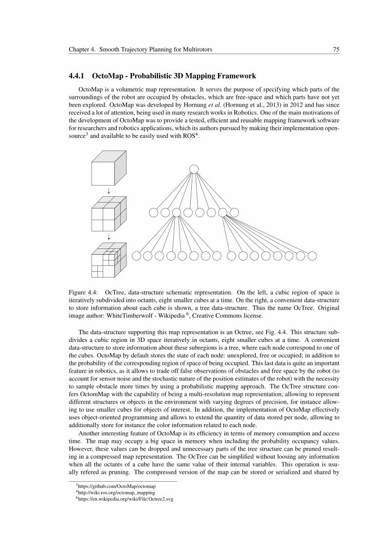
Chapter 4. Smooth Trajectory Planning for Multirotors 75
4.4.1 OctoMap - Probabilistic 3D Mapping Framework
OctoMap is a volumetric map representation. It serves the purpose of specifying which parts of thesurroundings of the robot are occupied by obstacles, which are free-space and which parts have not yetbeen explored. OctoMap was developed by Hornung et al. (Hornung et al., 2013) in 2012 and has sincereceived a lot of attention, being used in many research works in Robotics. One of the main motivations ofthe development of OctoMap was to provide a tested, efficient and reusable mapping framework softwarefor researchers and robotics applications, which its authors pursued by making their implementation open-source3 and available to be easily used with ROS4.
Figure 4.4: OcTree, data-structure schematic representation. On the left, a cubic region of space isiteratively subdivided into octants, eight smaller cubes at a time. On the right, a convenient data-structureto store information about each cube is shown, a tree data-structure. Thus the name OcTree. Originalimage author: WhiteTimberwolf - Wikipedia 6, Creative Commons license.
The data-structure supporting this map representation is an Octree, see Fig. 4.4. This structure sub-divides a cubic region in 3D space iteratively in octants, eight smaller cubes at a time. A convenientdata-structure to store information about these subregions is a tree, where each node correspond to one ofthe cubes. OctoMap by default stores the state of each node: unexplored, free or occupied; in addition tothe probability of the corresponding region of space of being occupied. This last data is quite an importantfeature in robotics, as it allows to trade off false observations of obstacles and free space by the robot (toaccount for sensor noise and the stochastic nature of the position estimates of the robot) with the necessityto sample obstacle more times by using a probabilistic mapping approach. The OcTree structure con-fers OctomMap with the capability of being a multi-resolution map representation; allowing to representdifferent structures or objects in the environment with varying degrees of precision, for instance allow-ing to use smaller cubes for objects of interest. In addition, the implementation of OctoMap effectivelyuses object-oriented programming and allows to extend the quantity of data stored per node, allowing toadditionally store for instance the color information related to each node.
Another interesting feature of OctoMap is its efficiency in terms of memory consumption and accesstime. The map may occupy a big space in memory when including the probability occupancy values.However, these values can be dropped and unnecessary parts of the tree structure can be pruned result-ing in a compressed map representation. The OcTree can be simplified without loosing any informationwhen all the octants of a cube have the same value of their internal variables. This operation is usu-ally refered as pruning. The compressed version of the map can be stored or serialized and shared by
3https://github.com/OctoMap/octomap4http://wiki.ros.org/octomap_mapping6https://en.wikipedia.org/wiki/File:Octree2.svg
76 4.4. Trajectory Planning - Theoretical Background
multiple autonomous agents, resulting in a reduced utilization of communication bandwidth. The Oc-toMap implementation provides a serialization interface that allows to send the compressed map so thatit can be shared between robots over bandwidth constrained networks, such as wireless over long dis-tances (Yanmaz et al., 2014). For more details, the reader is refered to the publication about OctoMap byHornung et al. (Hornung et al., 2013).
Various OctoMap representations have been shown already on this chapter: the simulation environ-ment of the EuRoC2014 autonomous flight challenge, see Fig. 4.1, and two maps obtained by using a fullvision-based Structure from Motion pipeline, see Sec. 4.3.1, that were utilized in the participation in the2016 DJI Developer Challenge, see Figs. 4.2 & 4.3.
4.4.2 Dynamic Efficient Obstacle Distance CalculationAs shown in Fig. 4.4, the OcTree representation of the environment subdivides the space in cubic
regions. A grid representation of the OcTree at a fixed resolution can be extracted, to which it is possibleto apply a distance transform resulting in a distance map to obstacles. The distance map is a matrix, fromwhich each value corresponds to a small cube in space at the mentioned fixed resolution. The value storesthe distance to the closest mapped obstacle in 3D space.
An implementation for Octomap of such an approach was developed by Lau et. al. (Lau et al., 2013)and released as open-source as a library named “DynamicEDT3D: A library for Incrementally UpdatableEuclidean distance transforms in 3D”. The code is available inside the OctoMap source-code repository.This distance map implementation is well tested and still supported in 2016. Its main characteristics arebeing compatible with 2D and 3D maps, time efficiency and being compatible with OctoMap.
This type of distance map is grown from the obstacle-space towards the interior of the free-space, upto a maximum desired distance (for computational efficiency reasons). Points further away from obstaclesare all filled in to be at this said maximum distance. The distance map can be updated incrementally whennew obstacles are located in the environment. Such incremental modifications to the distance map aredirectly performed after updates to the OctoMap representation.
Since the internal data-structure storing the distance map is basically an array, its access time is ex-tremely fast. This means that a node distance lookup requires constant time: checking whether a point inspace is occupied, collision checks, calculating the clearance of a patch from obstacles and the calculationof obstacle-free paths can be integrated very efficiently inside the motion planning algorithm.
In the present chapter, the distance map has been utilized to speed the calculation of obstacle-freepaths for quadrotor drones in relatively open outdoors environments. For more details about the Dynam-icEDT3D distance map implementation, the reader is refered to the publication (Lau et al., 2013).
4.4.3 Probabilistic RoadMap - Planning AlgorithmThis motion planning method solves the problem of finding an obstacle-free path between an start-
ing position and a goal position. The Probabilistic RoadMap (PRM) algorithm was proposed byKavraki et. al. (Kavraki et al., 1996). It is a sampling-based motion planning algorithm that works inthe configuration space of the robot, where each point corresponds to a fully defined position of the robotin 3D space.
The trajectory planning problem is separated in two phases: the roadmap construction phase and thequery phase. These two phases are depicted in Fig. 4.5. The roadmap construction is shown in the firstfive drawings of the figure, followed by an example of a query phase in the last drawing. The roadmap isbasically a graph where the nodes are feasible robot configurations and the edges represent simple motionprimitives that are only added when they are tested to be obstacle-free.
The PRM constitutes a multiple-query planning algorithm, i. e. it allows to solve multiple motionplanning queries potentially making the planning queries less computationally demanding as the roadmapgrows and becomes more complete. The queries are handled quite fast by first trying to connect thestarting and goal points to the roadmap, and then solving for the shortest path by using the A* Dijkstra’salgorithm (Dijkstra, 1959). If the starting or goal points cannot be added to the roadmap by simplemotion primitives, then the roadmap is grown with the objective of connecting these two points to it. Thedownside, is that the roadmap needs to be remade or at least updated after every update to the obstacle
8https://commons.wikimedia.org/wiki/File:Motion_planning_configuration_space_road_map_path.svg

Chapter 4. Smooth Trajectory Planning for Multirotors 77
Figure 4.5: Probabilistic roadmap (PRM), motion planning algorithm. The main insight of this algorithmis to construct a graph of connected points in the configuration space of the robot. The gray region showsthe obstacle-space, and the white the free-space. This graph sown by the nodes and edges in the figureis what is called the roadmap. Every edge represents obstacle-free paths. The graph is constructed byiteratively randomly sampling points in the configuration space of the robot, and trying to connect tonearby points and to the current roadmap by simple motion primitives. The first five drawings depict theroadmap construction. The last drawing shows how the roadmap can be used to quite fast answer to newmotion queries by using the A* Dijkstra’s shortest path algorithm (Dijkstra, 1959). Original image author:Simeon87 - Wikipedia8, Creative Commons license.
map, as priorly obstacle-free edges and feasible nodes of the graph might become occluded by newlylocated obstacles. This fact limits the advantages of the multiple-query capability in applications wherethe obstacle map needs to be explored in real-time or in presence of dynamic obstacles.
The PRM sampling-based motion planning algorithm is proven to have very good statistical propertieswith regards to the motion planning objective. The PRM algorithm is probabilistically complete, meaningthat given that there is a solution path for the current motion planning query, then the PRM method ensuresthat given enough time to perform the calculation it can find a feasible solution path. In addition, if thepoints in the configuration space have a good visibility, meaning that there not many obstacles with smallbottlenecks, then a solution to the motion planning query will be found in a relatively short time.
The algorithm utilized in our work is the PRM* (Karaman et al., 2011), which is an improvement onthe PRM. It allows not only to find a solution path to the motion planning query, but it also converges tothe minimum cost optimal solution. We utilized the open-source implementation from the Open MotionPlanning Library (OMPL) (Sucan et al., 2012).
4.4.4 Rapidly-Exploring Random Trees - Planning AlgorithmThis motion planning method solves the problem of finding an obstacle-free path between an starting
position and a goal position. The Rapidly-Exploring Random Trees (RRT) algorithm was proposed byLavalle in 1998 et. al. (LaValle, 1998). It is a sampling-based motion planning algorithm that works inthe configuration space of the robot, where each point corresponds to a fully defined position of the robotin 3D space.
The main insight to this algorithm lies in the creation of a tree shaped graph that tends to fill in all thefree-space available to the robot for navigation. The interpretation of the graph is similar to that of the
10https://commons.wikimedia.org/wiki/File:Rapidly-exploring_Random_Tree_(RRT)_500x373.gif

78 4.4. Trajectory Planning - Theoretical Background
Figure 4.6: Rapidly-exploring random tree (RRT), motion planning algorithm. These drawings show howthis planning algorithm grows a tree-shaped connected graph of feasible states by means of obstacle-freepaths. In this case there are no obstacles. The purpose of the figure is to show how the nodes are sampled,and how they tend to explore the whole free-space. The RRT is a single-query algorithm. Original imageauthor: Javed Hossain - Wikipedia10, Creative Commons license.
roadmap in the PRM. Nodes correspond to feasible positions and edges to obstacle-free simple motionprimitives between nodes. The tree is grown by randomly sampling points in the configuration space ofthe robot. The algorithm tries to connect each new sample to the current RRT tree. The growth of an RRTtree in a region with no obstacles is depicted in Fig. 4.6. The tree is grown from the starting position ofthe motion planning query, and every certain number of samples the algorithm will try to connect the goalpoint to the tree. At this point, a feasible path is returned as solution solution to the query. This methodsis a single-query algorithm, and it is very well suited to applications where the obstacle map is updated inreal-time.
The RRT sampling-based motion planning algorithm, similarly to the PRM, is also proven to havevery good statistical properties with regards to the motion planning objective. For instance the RRT isproven to be probabilistically complete.
The algorithm utilized in our work is the RRT* (Karaman et al., 2011), which is an improvement onthe RRT. It allows not only to find a solution path to the motion planning query, but it also converges tothe minimum cost optimal solution. We utilized the open-source implementation from the Open MotionPlanning Library (OMPL) (Sucan et al., 2012).
4.4.5 Utilized open-source librariesThese are the utilized external software libraries:
• Octomap: map representation, see Sec. 4.4.1
• ROS octomap_mapping package11: visualization in Rviz.
• DynamicEDT3DOctomap: this library delivers a clearance distance map for every cell in the map,see Sec. 4.4.2.
• OMPL - Open Motion Planning Library: PRM* and RRT* planning algorithms, seeSecs. 4.4.3 & 4.4.4. This library was selected because it is used in the MoveIt community in ROS,and also because it is under active development.
• Eigen3 library12: for matrix operations.11https://github.com/OctoMap/octomap_mapping12http://eigen.tuxfamily.org/
Chapter 4. Smooth Trajectory Planning for Multirotors 79
4.5 Obstacle-free Smooth Trajectory Planning
The main calculations realized during the operation of the trajectory planner are the following:
1. Planer initialization.
2. Answering to planning queries.
(a) Geometric Trajectory Planning.
(b) Geometric Trajectory Shortening and Smoothing.
(c) Speed planning along the trajectory.
The following information is also provided in this section:
• Communication with other modules
• Configuration Parameters
4.5.1 Planner initialization
1. Open the file that contains the octomap representation of the static map/environment.
2. The map is stored as a octomap octree (low memory consumption) and as aDynamicEDT3DOctomap distance map (high memory consumption). Every cell of the dis-tance map contains the location of the nearest obstacle and the distance to it (or clearance).
3. Trajectory planner object initialization, the type depends on the kind of environment under consid-eration:
(a) Static: the PRM* planning algorithm is used. The RoadMap of the planner is initialized witha prefixed number of nodes.
(b) Dynamic: the RRT* planning algorithm is used. The trajectories are calculated in a single-query fashion using the latest version of the Octomap, which is updated with the latest obstacledata, for instance using depth maps acquired with a stereo camera.
4.5.2 Obstacle-aware Geometric Trajectory Planning
The trajectory planning is performed in 3D space (no attitude angles, only position), assuming thatthe quadrotor is omnidirectional (it can move at any point in any direction) using the PRM* or the RRT*algorithms. In this step a cost function is evaluated over candidate paths and the delivered trajectory isof minimum cost. The cost penalizes length, proximity to obstacles and changes in the altitude of thetrajectory. Ideally the trajectory is preferred to, in this order, not have unnecessary changes in altitude, notbe unnecessarily near obstacles and be as short as possible.
The trajectory queries are from the current pose estimate as starting point to the goal position. Thecollision check is performed using the DynamicEDT3D distance map, which was is very fast in run-time.The collision check is done recursively from bigger to smaller parts of the quadrotor bounding box. If thenearest obstacle is nearer than the size of the currently evaluated bounding box, then the 8 neighbouringsub-bouding boxes are checked and so on.
A cost function is used to assign a cost to the obstacle-free trajectories that are a valid solution to theplanning query. The cost function evaluates:
• Changes in altitude between consecutive waypoints: a more horizontal trajectory is preferred.
• Clearance to nearby obstacles : higher clearance is preferred.
• Path length : shorter paths are preferred.
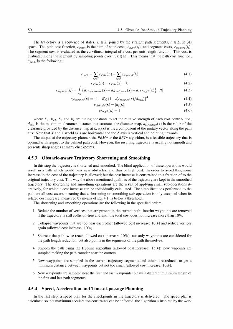
80 4.5. Obstacle-free Smooth Trajectory Planning
The trajectory is a sequence of states, si ∈ S, joined by the straight path segments, li ∈ L, in 3Dspace. The path cost function, cpath, is the sum of state costs, cstate(si), and segment costs, csegment(li).The segment cost is evaluated as the curvilinear integral of a cost per unit length function. This cost isevaluated along the segment by sampling points over it, x ∈ R3. This means that the path cost function,cpath, is the following:
cpath = ∑si∈S
cstate(si)+ ∑li∈L
csegment(li) (4.1)
cstate(si) = cstate(x) = 0 (4.2)
csegment(li) =∫
li
{Kc cclearance(x)+Ka caltitude(x)+Kl clength(x)
}|dl| (4.3)
cclearance(x) = {1+Kc2 (1−dclearance(x)/dmax)}4 (4.4)caltitude(x) = |uz(x)| (4.5)
clength(x) = 1 (4.6)
where Kc, Kc2, Ka and Kl are tuning constants to set the relative strength of each cost contribution,dmax is the maximum clearance distance that saturates the distance map, dclearance(x) is the value of theclearance provided by the distance map at x, uz(x) is the z component of the unitary vector along the pathat x. Note that X and Y world axis are horizontal and the Z axis is vertical and pointing upwards.
The output of the trajectory planner, the PRM* or the RRT* algorithm, is a feasible trajectory that isoptimal with respect to the defined path cost. However, the resulting trajectory is usually not smooth andpresents sharp angles at many checkpoints.
4.5.3 Obstacle-aware Trajectory Shortening and SmoothingIn this step the trajectory is shortened and smoothed. The blind application of these operations would
result in a path which would pass near obstacles, and thus of high cost. In order to avoid this, someincrease in the cost of the trajectory is allowed; but the cost increase is constrained to a fraction of to theoriginal trajectory cost. This way the above mentioned qualities of the trajectory are kept in the smoothedtrajectory. The shortening and smoothing operations are the result of applying small sub-operations it-eratively, for which a cost increase can be individually calculated. The simplifications performed to thepath are all cost-aware, meaning that a shortening or smoothing sub-operation is only accepted when itsrelated cost increase, measured by means of Eq. 4.1, is below a threshold.
The shortening and smoothing operations are the following in the specified order:
1. Reduce the number of vertices that are present in the current path: interim waypoints are removedif the trajectory is still collision-free and until the total cost does not increase more than 10%.
2. Collapse waypoints that are too near each other (allowed cost increase: 10%) and reduce verticesagain (allowed cost increase: 10%)
3. Shortcut the path twice (each allowed cost increase: 10%): not only waypoints are considered forthe path length reduction, but also points in the segments of the path themselves.
4. Smooth the path using the BSpline algorithm (allowed cost increase: 15%): new wapoints aresampled making the path rounder near the corners.
5. New waypoints are sampled in the current trajectory segments and others are reduced to get aminimum distance between waypoints but not too small (allowed cost increase: 10%).
6. New waypoints are sampled near the first and last waypoints to have a different minimum length ofthe first and last path segments.
4.5.4 Speed, Acceleration and Time-of-passage PlanningIn the last step, a speed plan for the checkpoints in the trajectory is delivered. The speed plan is
calculated so that maximum acceleration constraints can be enforced, the algorithm is inspired by the work

Chapter 4. Smooth Trajectory Planning for Multirotors 81
of Hoffman. et al. (Hoffmann, Gabriel M et al., 2008), but with improvements. A speed plan is calculatediteratively to obtain an acceleration plan whose derivative is bounded. The speed plan calculation isperformed by the following steps, in the specified order:
1. Geometric calculations are performed to estimate the tangent, normal and binormal vectors at eachwaypoint.
2. Then, the radius of curvature in each waypoint is calculated:
• A system of equations to determine the circumference that approximates each waypoint[i] andits neighbours is calculated.
• For each point[i], its neighbours are projected into the plane formed by the normal and tangentvectors estimated at point[i].
• The radius of curvature in each waypoint is calculated and the tangent and normal are cor-rected based on the solution of the system of equations.
Steps 1 & 2 amount to the following calculations. For each point, pi. First, Nnc neighboring points,pni j, are sampled around, pi, each one separated by a predefined distance dnc to pi or to anotherneighbor, pni j. By this definition, pni0 = pi and for j < 0 ( j > 0) the point pni j is before (after) pi inthe trajectory path. Second, see Eqs. 4.7 & 4.8 & 4.9, the tangent, ti, binormal, bi, and normal, ni,of the trajectory at point pi are estimated by calculating mean values using the Nnc neighbors pni jaround the point i, pi:
ti j =pni j+1−pni j
|pni j+1−pni j|with j =
{−Nnc
2,−Nnc
2+1, . . . ,
Nnc
2−1}
ti =∑ j ti j
Nnc; ti =
ti
|ti|(4.7)
bi j = ti j× ti( j+1) with j ={−Nnc
2,−Nnc
2+1, . . . ,
Nnc
2−2}
bi =∑ j bi j
Nnc−1; bi =
bi
|bi|(4.8)
ni j = bi j× ti j with j ={−Nnc
2,−Nnc
2+1, . . . ,
Nnc
2−2}
ni =∑ j ni j
Nnc−1; ni =
ni
|ni|(4.9)
And third, the radius of curvature ri at the point pi is calculated. In order to perform the estimationof this value, the Nnc neighbors are projected onto the plane defined by the tangent, ti, and normal,ni, vectors of the trajectory at the point pi. Then, see Eqs. 4.10 & 4.11 & 4.12, their 2D coordinates{
xi j,yi j}
on this plane are used to solve the following system of equations. It provides an estimate ofthe radius of curvature ri, and the corresponding center of curvature, ci or
{cxi,cyi
}, at the point pi.
This is also used to obtain a better estimate of the normal and tangent vectors, n∗i and t∗i , which areused in the rest of the calculations.
xi j = (pni j−pi) · ti yi j = (pni j−pi) ·ni (4.10)[xi j yi j 1...
......
] −2cxi−2cyi
c2xi + c2
yi− r2i
=
[−x2
i j− y2i j
...
]
with j ={−Nnc
2,−Nnc
2+1, . . . ,
+Nnc
2
}(4.11)
n∗i =cxiti + cyini
|cxiti + cyini|t∗i = n∗i ×bi (4.12)

82 4.5. Obstacle-free Smooth Trajectory Planning
Configuration values for this calculation that have worked well in our experiments are Nnc = 8 anddnc = 0.50m. Predefined result values are used for special cases. For instance, when all the Nncneighboring points around waypoint j are aligned in a straight line, then its radius of curvature isset to a high value for the rest of the algorithm.
3. The main configuration of the algorithm consists of the maximum upwards, downwards and hori-zontal velocities and accelerations. These values are used to calculate the maximum velocity andacceleration as a function of a unitary direction vector, see Algs. 3 & 4. Note that in Algs. 3 & 4the maximum velocity and acceleration constraints are set by an ellipsoid so as to make the outputof these functions continuous with respect to the trajectory direction.
4. The desired speed for the trajectory is set at every point to the minimum of the followingtwo values: (1) the maximum configured velocity Velocity_Max_Direction, see Alg. 3, and(2) the maximum attainable velocity set by the radius of curvature vmax,i =
√amax,n · ri whereamax,n = Acceleration_Max_Direction(n∗i ,config) , see Alg. 4. Then, the desired initial and finalvelocities are set, which are usually both set to zero.
5. A first speed plan is calculated that complies with the acceleration constraints. This algorithm,that we are going to call velocity_plan_sweep_double_pass, see Alg. 1, was implemented follow-ing the publication (Hoffmann, Gabriel M et al., 2008) with only minor modifications. Note thatthe equations relating path trajectory lengths, velocities and accelerations correspond to those oflinear uniformly accelerated motion (for every section of the trajectory). The modifications to thisalgorithm are: (1) see line 3 of Alg. 2 and (2) Algs. 3 & 4. Later on, a velocity smoothing stepis proposed that provides a much more continuous and feasible acceleration plan than proposed byHoffman et al. in (Hoffmann, Gabriel M et al., 2008). For a comparison between smoothed andnon-smoothed speed-plans, the reader is referred to Sec. 4.7.3.1.
Algorithm 1 Velocity_Plan_Sweep_Double_Pass(s,r,{t∗i }i ,vdesired ,config
)1: vplan = vdesired2: vinit ← vdesired,13: vend ← vdesired,N4: flip
{s,r,{t∗i }i ,vdesired ,vplan
}: /* the flip function flips, or interchanges, the elements of each vector,
so that they are time-wise reversed */5: s = (−1) · s6:{
vplan,aat,plan,∆∆∆tplan}= Velocity_Plan_Sweep
(vend ,s,vplan,r,{t∗i }i ,config
); /* see Alg. 2 */
7: flip{
s,r,{t∗i }i ,vdesired ,vplan}
8: s = (−1) · s9:{
vplan,aat,plan,∆∆∆tplan}= Velocity_Plan_Sweep
(vinit ,s,vplan,r,{t∗i }i ,config
)10: return
{vplan,aat,plan,∆∆∆tplan
}; /* note that the cross-track acceleration is act,plan =
[v2
plan,i/ri
]*/

Chapter 4. Smooth Trajectory Planning for Multirotors 83
Algorithm 2 Velocity_Plan_Sweep(vinit ,s,v,r,{t∗i }i ,config
)1: v1← vinit2: for i = 1 to N do3: amax = Acceleration_Max_Direction(t∗i ,config)− v2
iri
; /* see Alg. 4 */
4: aat,i←min(
amax,v2
i −(vi+1)2
2(si−si+1)
)5: if aat,i > 0 then
6: vi+1←√
v2i −2aat,i(si− si+1)
7: ∆ti←−vi+√
v2i −2aat,i(si−si+1)
aat,i
8: else9: if vi > vi+1 then
10: vi+1← vi+1
11: aat,i←v2
i −v2i+1
2(si−si+1)
12: ∆ti←−vi+√
v2i −2aat,i(si−si+1)
aat,i
13: else14: vi+1← vi15: aat,i← 016: ∆ti← (si+1−si)
vi17: end if18: end if19: end for20: return
{vplan = v,aat,plan,∆∆∆tplan
}; // note that the cross-track acceleration is act,plan =
[v2
plan,i/ri
]
Algorithm 3 Velocity_Max_Direction(d,config)1: vmax,h = vmax,xy2: if dz > 0 then3: vmax,v = vmax,z,up4: else5: vmax,v = vmax,z,down6: end7: vmax,d =
vmax,hvmax,v√v2
max,v(d2x+d2
y )+v2max,hd2
z
8: return vmax,d
Algorithm 4 Acceleration_Max_Direction(d,config)1: amax,h = amax,xy2: if dz > 0 then3: amax,v = amax,z,up4: else5: amax,v = amax,z,down6: end7: amax,d =
amax,hamax,v√a2
max,v(d2x+d2
y )+a2max,hd2
z
8: return amax,d
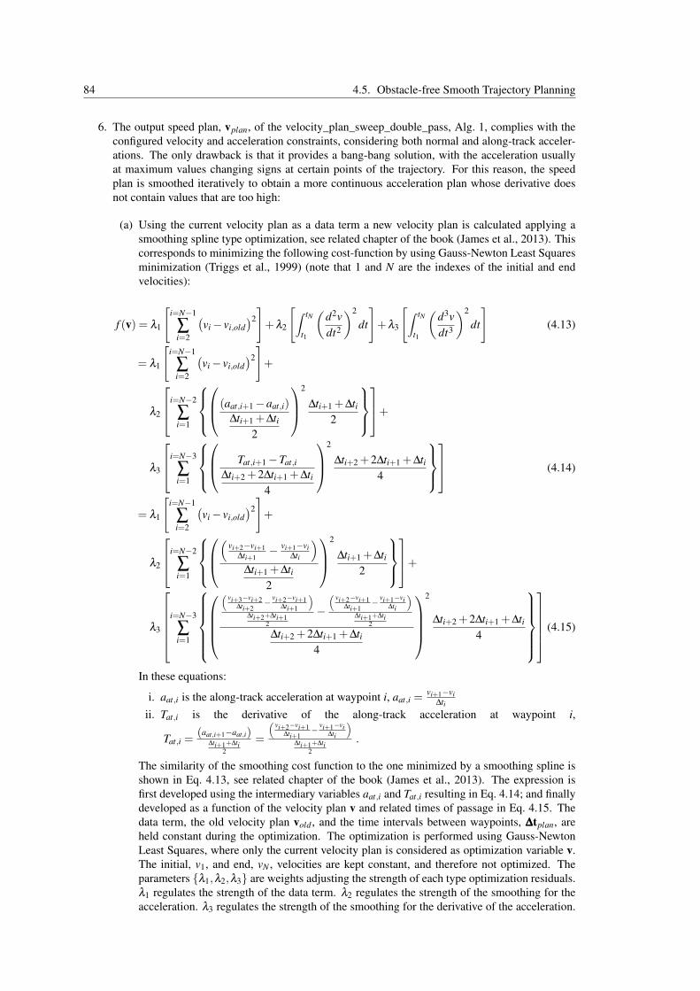
84 4.5. Obstacle-free Smooth Trajectory Planning
6. The output speed plan, vplan, of the velocity_plan_sweep_double_pass, Alg. 1, complies with theconfigured velocity and acceleration constraints, considering both normal and along-track acceler-ations. The only drawback is that it provides a bang-bang solution, with the acceleration usuallyat maximum values changing signs at certain points of the trajectory. For this reason, the speedplan is smoothed iteratively to obtain a more continuous acceleration plan whose derivative doesnot contain values that are too high:
(a) Using the current velocity plan as a data term a new velocity plan is calculated applying asmoothing spline type optimization, see related chapter of the book (James et al., 2013). Thiscorresponds to minimizing the following cost-function by using Gauss-Newton Least Squaresminimization (Triggs et al., 1999) (note that 1 and N are the indexes of the initial and endvelocities):
f (v) = λ1
[i=N−1
∑i=2
(vi− vi,old
)2
]+λ2
[∫ tN
t1
(d2vdt2
)2
dt
]+λ3
[∫ tN
t1
(d3vdt3
)2
dt
](4.13)
= λ1
[i=N−1
∑i=2
(vi− vi,old
)2
]+
λ2
i=N−2
∑i=1
(aat,i+1−aat,i)
∆ti+1 +∆ti2
2
∆ti+1 +∆ti2
+
λ3
i=N−3
∑i=1
Tat,i+1−Tat,i
∆ti+2 +2∆ti+1 +∆ti4
2
∆ti+2 +2∆ti+1 +∆ti4
(4.14)
= λ1
[i=N−1
∑i=2
(vi− vi,old
)2
]+
λ2
i=N−2
∑i=1
(
vi+2−vi+1∆ti+1
− vi+1−vi∆ti
)∆ti+1 +∆ti
2
2
∆ti+1 +∆ti2
+
λ3
i=N−3
∑i=1
( vi+3−vi+2
∆ti+2− vi+2−vi+1
∆ti+1
)∆ti+2+∆ti+1
2
−( vi+2−vi+1
∆ti+1− vi+1−vi
∆ti
)∆ti+1+∆ti
2
∆ti+2 +2∆ti+1 +∆ti4
2
∆ti+2 +2∆ti+1 +∆ti4
(4.15)
In these equations:
i. aat,i is the along-track acceleration at waypoint i, aat,i =vi+1−vi
∆tiii. Tat,i is the derivative of the along-track acceleration at waypoint i,
Tat,i =(aat,i+1−aat,i)
∆ti+1+∆ti2
=
( vi+2−vi+1∆ti+1
− vi+1−vi∆ti
)∆ti+1+∆ti
2
.
The similarity of the smoothing cost function to the one minimized by a smoothing spline isshown in Eq. 4.13, see related chapter of the book (James et al., 2013). The expression isfirst developed using the intermediary variables aat,i and Tat,i resulting in Eq. 4.14; and finallydeveloped as a function of the velocity plan v and related times of passage in Eq. 4.15. Thedata term, the old velocity plan vold , and the time intervals between waypoints, ∆∆∆tplan, areheld constant during the optimization. The optimization is performed using Gauss-NewtonLeast Squares, where only the current velocity plan is considered as optimization variable v.The initial, v1, and end, vN , velocities are kept constant, and therefore not optimized. Theparameters {λ1,λ2,λ3} are weights adjusting the strength of each type optimization residuals.λ1 regulates the strength of the data term. λ2 regulates the strength of the smoothing for theacceleration. λ3 regulates the strength of the smoothing for the derivative of the acceleration.
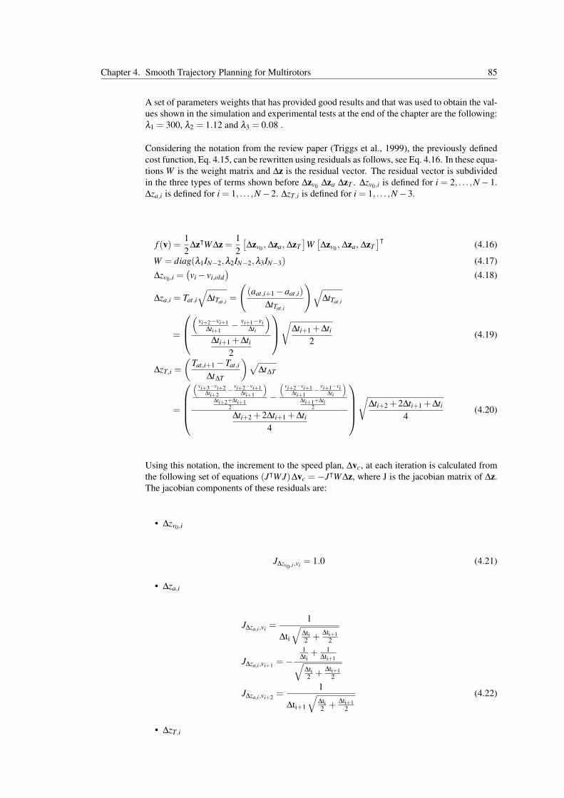
Chapter 4. Smooth Trajectory Planning for Multirotors 85
A set of parameters weights that has provided good results and that was used to obtain the val-ues shown in the simulation and experimental tests at the end of the chapter are the following:λ1 = 300, λ2 = 1.12 and λ3 = 0.08 .
Considering the notation from the review paper (Triggs et al., 1999), the previously definedcost function, Eq. 4.15, can be rewritten using residuals as follows, see Eq. 4.16. In these equa-tions W is the weight matrix and ∆z is the residual vector. The residual vector is subdividedin the three types of terms shown before ∆zv0 ∆za ∆zT . ∆zv0,i is defined for i = 2, . . . ,N− 1.∆za,i is defined for i = 1, . . . ,N−2. ∆zT,i is defined for i = 1, . . . ,N−3.
f (v) =12
∆zᵀW∆z =12[∆zv0 , ∆za, ∆zT
]W[∆zv0 , ∆za, ∆zT
]ᵀ (4.16)
W = diag(λ1IN−2,λ2IN−2,λ3IN−3) (4.17)∆zv0,i =
(vi− vi,old
)(4.18)
∆za,i = Tat,i
√∆tTat,i =
((aat,i+1−aat,i)
∆tTat,i
)√∆tTat,i
=
(
vi+2−vi+1∆ti+1
− vi+1−vi∆ti
)∆ti+1 +∆ti
2
√∆ti+1 +∆ti2
(4.19)
∆zT,i =
(Tat,i+1−Tat,i
∆t∆T
)√∆t∆T
=
( vi+3−vi+2
∆ti+2− vi+2−vi+1
∆ti+1
)∆ti+2+∆ti+1
2
−( vi+2−vi+1
∆ti+1− vi+1−vi
∆ti
)∆ti+1+∆ti
2
∆ti+2 +2∆ti+1 +∆ti4
√
∆ti+2 +2∆ti+1 +∆ti4
(4.20)
Using this notation, the increment to the speed plan, ∆vc, at each iteration is calculated fromthe following set of equations (JᵀWJ)∆vc = −JᵀW∆z, where J is the jacobian matrix of ∆z.The jacobian components of these residuals are:
• ∆zv0,i
J∆zv0,i,vi = 1.0 (4.21)
• ∆za,i
J∆za,i,vi =1
∆ti√
∆ti2 +
∆ti+12
J∆za,i,vi+1 =−1
∆ti+ 1
∆ti+1√∆ti2 +
∆ti+12
J∆za,i,vi+2 =1
∆ti+1
√∆ti2 +
∆ti+12
(4.22)
• ∆zT,i

86 4.5. Obstacle-free Smooth Trajectory Planning
J∆zT,i,vi =−1
∆ti(
∆ti2 +
∆ti+12
)√∆ti4 +
∆ti+12 +
∆ti+24
J∆zT,i,vi+1 =
1∆ti+1
(∆ti+1
2 +∆ti+2
2
) + 1∆ti
+ 1∆ti+1
∆ti2 +
∆ti+12√
∆ti4 +
∆ti+12 +
∆ti+24
J∆zT,i,vi+2 =−
1∆ti+1
(∆ti2 +
∆ti+12
) + 1∆ti+1
+ 1∆ti+2
∆ti+12 +
∆ti+22√
∆ti4 +
∆ti+12 +
∆ti+24
J∆zT,i,vi+3 =1
∆ti+2
(∆ti+1
2 +∆ti+2
2
)√∆ti4 +
∆ti+12 +
∆ti+24
(4.23)
(b) After every iteration of the smoothing spline optimization the resulting speed plan is not self-consistent. That means that the values
{vplan,aat,plan,∆∆∆tplan
}do not verify the equations of an
uniformly accelerated motion for all segments of the trajectory. This is because the smoothingprocedure does not enforce them. For this reason, after every iteration of the smoothing splineoptimization a new pass of velocity_plan_sweep_double_pass is performed, so that a new setof self-consistent values for
{vplan,aat,plan,∆∆∆tplan
}is obtained. This amounts to the following
function call:[vplan,aat,plan,∆∆∆tplan
]= Velocity_Plan_Sweep_Double_Pass
(s,r,{t∗i }i ,vnewmax,config
)Where vnewmax is defined for every component as the minimum of vplan +∆vc and vdesired ,that is: vnewmax =
{vnewmax,i = min
(vplan,i +∆vc,i,vdesired,i
)}.
The Gauss-Newton Least Squares optimization, that encodes velocity smoothing, is stopped:when (1) the norm of the jacobian of the cost function, f (v) increased in the last iteration or(2) when a preset number of iterations, 10 provides consistently good results, is reached.
(c) Rerunning the smoothing spline optimization exchanging the data term by the last smoothedvelocity plan allows the algorithm to gradually forget the strong initial bang-bang velocityplan. For a given set of the smoothing strength parameters {λ1,λ2,λ3}, increasing the numberof reruns of the smoothing spline optimization results in smoother speed plans, with lowermaximum values for the acceleration derivative. This effect is demonstrated in the results sec-tion, see Sec. 4.7.3.2. This fact allows to calculate a speed plan with an acceleration derivativebounded by a certain value. In practice, in order to obtain efficient computation times, thesmoothing spline optimization is repeated a fixed number of times. In our experiments 10provides consistently good results, see Secs. 4.7.3.3 & 4.7.4.1.
The velocity smoothing operation is summarized in Alg. 5:
7. The calculated trajectory message for the trajectory controller is filled-in including the speed andacceleration plans. This is the final trajectory which is to be executed by the trajectory controller.Take into account that the trajectory controller, used in both in EuRoC and the DJI Challenge,calculates a smoother trajectory by fitting a spline to the provided trajectory, times-of-passage,speed and acceleration plans.
4.5.5 Communication with other modulesOur trajectory planner ROS node communicates using the following topics:
• Subscription to the goal position.
• Subscription to the current pose estimate.
• Subscription to the depth maps of the stereo cameras on the drone. The depth data is used to updatethe planner’s internal map representation.

Chapter 4. Smooth Trajectory Planning for Multirotors 87
Algorithm 5 Velocity_Smoothing(s,r,{t∗i }i ,vplan,∆tplan,r
)1: for i = 1 to num_passes do2: vold = vplan3: for j = 1 to max_iterations_per_pass do
4:
{∆vc,
∣∣∣ d fdv
∣∣∣j
}= velocity_smoothing_optimization_iteration
(vplan,vold ,∆∆∆tplan,r
)5: if
(( j == 1) or
(∣∣∣ d fdv
∣∣∣j<∣∣∣ d f
dv
∣∣∣j−1
))6: vnewmax = min
(vplan +∆vc,vdesired
)={
vnewmax,i = min(vplan,i +∆vc,i, vdesired,i
)}7:
[vplan,aat,plan,∆∆∆tplan
]= Velocity_Plan_Sweep_Double_Pass
(s,r,{t∗i }i ,vnewmax,config
)8: else9: break
10: end if11: end for; /* j */12: end for; /* i */13: return
{vplan,aat,plan,∆∆∆tplan
}; /* note that the cross-track acceleration is act,plan =
[v2
plan,i/ri
]*/
• Publication of the calculated trajectory, which includes the waypoints and the corresponding times-of-passage, acceleration and speed plans.
4.5.6 Configuration ParametersThe most important parameters are the following:
• Desired maximum velocity over the trajectory (vertical upwards and downwards; and horizontal).
• Desired maximum acceleration over the trajectory (vertical upwards and downwards; and horizon-tal).
• Maximum clearance distance, dmax, calculated by the DynamicEDT3D library. Points at furtherdistances are simply set to this maximum value, therefore reducing the computation requirementsof the distance map calculation.
• The multirotor’s horizontal and vertical sizes in m.
• The maximum planning time in seconds allocated for the calculation of an obstacle free trajectoryby the OMPL library.
• Maximum distance between waypoints in the output trajectory.
• For the PRM* algorithm, the minimum number of nodes calculated to populate the free space duringthe planner initialization.
• The parameters {λ1,λ2,λ3} that adjust the weights of each type of optimization residuals of thevelocity smoothing operation.
4.6 Geometric Speed PlannerThe previous section, Sec. 4.5 “Obstacle-free Smooth Trajectory Planning”, described a planning
approach which divides the problem in separate subproblems: obstacle-free path planning, obstacle-awaretrajectory shortening and smoothing and speed planning. The presented speed planning approach can alsobe used when the drone needs to fly in obstacle-free areas over paths defined by waypoints. For thispurpose, a module named “Geometric Speed Planner” was developed. In the obstacle-free scenario, thismodule serves as an interface to the controller which is expecting as trajectory a path supplemented witha speed, an acceleration and a time-of-passage plans. The “Geometric Speed Planner” implements onlythe following two subproblems: trajectory smoothing and speed planning. These steps correspond to thefollowing:

88 4.7. Experimental Results
1. Trajectory smoothing with no cost-checking:
1. Add waypoints in the current path until the path segments are all smaller than a given smalldistance, for instance 1m. Then, reduce consecutive waypoints that are too near each otherat less distance than a given value, for instance 7m. This has the effect of dividing sharptrajectory corners into two or more softer corners, which helps in the next step.
2. Smooth the path using the BSpline algorithm (for instance 6 passes): new wapoints are sam-pled making the path rounder near the corners.
3. Reduce consecutive waypoints that are too near each other at less distance than a given value,for instance 1.5m. This reduces the number of waypoints that are sampled very close to eachother.
4. Reduce consecutive waypoints that are in a straight line and too near each other at less distancethan a given value, for instance 5.0m. This is important to reduce the number of points overwhich the speed plan is calculated, and also the time that the controller needs to calculate theinterpolating spline over the trajectory.
5. The first and last trajectory segments are subdivided two times to increase the number ofwaypoints for the initial and final accelerations, which is helpful for the subsequent speedplanning approach.
2. Speed planning: the algorithm explained in Sec. 4.5.4 is used.
4.7 Experimental Results
4.7.1 Videos of ExperimentsThe following videos show a multirotor in real and simulated flight executing trajectories delivered by
the presented trajectory planner:
• 2016 DJI Developer Challenge (DJIC 2016), http://bit.ly/2faublQ : this video summa-rizes the participation of the “Graz Griffins” team in the challenge. Starting at 2:38, first, someplanned trajectories and, second, the experimental autonomous flight where the trajectories plottedin Sec. 4.7.4 were executed are shown.
• An experimental fully autonomous package delivery flight demonstration made by theICG - TU Graz, https://youtu.be/bxM6dls2wuo:this demo was made in collaborationwith the company SFL Technologies as part of the roll-out of their brand new electric vehicle,the ELI. The roll-out of this vehicle and the autonomous flight demo have been described by twoAustrian newspapers: Mein Bezirk13 and Kleine Zeitung14.
• European Robotics Challenge (EuRoC 2014), https://bit.ly/2cQnO6I : this video showsthe performance of a simulated Asctec Firefly hexacopter MAV executing trajectories produced bythe presented planner by means of a controller developed by D. Muschick, a colleague from theInstitute of Automation and Control - TU Graz. Both algorithms where succinctly described in thepaper (Pestana et al., 2015).
4.7.2 Experimental Setup4.7.2.1 Flights in a Simulation Environment
The trajectory planner was first tested using the octomap map provided by the EuRoC2014 organizers.The Simulation Contest of EuRoC Challenge 3 takes places in a simulated outdoors industry environmentof size 50mx50mx40m, see Fig. 4.1; which is described using an Octomap with a leaf size of 0.25m. Thequadrotor has a diameter of (actually less than) 1.00m and a height of (actually less than) 0.50m. Fortask 4.3 of the simulation contest, the trajectories had to be calculated rather fast and executed at average
13ELI roll-out - Mein Bezirk - http://bit.ly/2hott8t14ELI roll-out - Kleine Zeitung - http://bit.ly/2it6N2P

Chapter 4. Smooth Trajectory Planning for Multirotors 89
speeds of around 3.5m/s to attain the best score in the simulation contest. The overall trajectory planningand execution had to be done in less than 10 seconds.
The feasibility of the calculated speed and acceleration plans were then tested in simulation, on theaccompanying simulator. A publication explaining the implementation, capabilities, and configuration ofthis simulator, the RotorS simulator framework (Furrer et al., 2016)15, has been published in 2016. Themain feature of the RotorS simulator are that it utilizes the Gazebo physics engine, that it can be easilyrun and interfaced using ROS, that it provides a controller and a state estimator to help the user gettingstarted, and that it provides an already implemented evaluation framework. For instance, the propellers aremodeled separately, so that multirotors with different number of propellers can be meaningfully simulated.There are currently a few MAVs available in the simulator: the AR Drone; the Asctec Firefly, Pelican andHummingbird and the 3D Robotics Iris.
It is noted here that there are other open-source multirotor drone simulators, among others: the hec-tor_quadrotor (Meyer et al., 2012)16, hardware and software in the loop simulators for the Pixhawk au-topilot1718 and the AirSim simulator19 (Shah et al., 2017) from Microsoft Research.
4.7.2.2 Experimental Flights with a Multirotor
The experimental flights were done as part of the participation on the 2016 DJI Developer Challenge,and they have been performed using a DJI M100 quadrotor drone. Our fully equipped DJI M100 quadrotorincludes: the DJI Manifold onboard computer, the DJI Guidance sensing system and the DJI Zenmuse X3gimbal camera. For more details on the used setup the reader is referred to Appx. H.3.1.
4.7.3 Results in EuRoC 2014 - Challenge 3 - Simulation ContestThe trajectory planner used in the participation of the “Graz Griffins” to the EuRoC 2014 challenge
utilized the PRM* planning algorithm. The performance characteristics of the planner are the following:
• Selected planning algorithm: PRM*.
• Memory usage:
– 300MB = 200MB map representations + 100MB [20.000 nodes] in planner data
– 633MB = 200MB map representations + 433MB [100.000 nodes] in planner data
• 20.000 nodes were used for the final submission. New nodes are created with each trajectoryplanning task. When there are too many nodes in the data structure the planner becomes slower inanswering individual queries.
• The loading time of the planner in the laptop Intel Core i7-4710HQ processor @ 2.5 GHz for 100knodes is around 50-70seconds.
• The planner is set to execute as a low priority process.
• The total computation time is around 0.7−1.2 s. This time is used as follows: 0.5 s for planning,0.1 s for trajectory simplification and 0.3 s for speed planning; resulting in a mean planning time ofaround 0.9 s.
• Main configuration parameters:
– dmax approximately set a desired safety distance to be kept between the MAV and the en-vironment. A wall can be approached as much as needed (for instance if the goal target isnear obstacles). However, the planner won’t do this unless needed and will stay away fromobstacles otherwise. This parameter was set to 4.0m.
15https://github.com/ethz-asl/rotors_simulator16http://wiki.ros.org/hector_quadrotor17http://ardupilot.org/dev/docs/sitl-simulator-software-in-the-loop.html18https://pixhawk.org/users/hil19https://github.com/Microsoft/AirSim

90 4.7. Experimental Results
– One of the last trajectory simplification steps resamples the trajectory before performing thespeed planning and delivering both to the Trajectory Controller. It sets the minimum (desired)distance between trajectory waypoints. This parameters was set to 1.0 m.
The evaluation of the EuRoC2014 organizers showed that the control framework developed byD. Muschick (Holzmann et al., 2015; Pestana et al., 2015) for the “Graz Griffins” team achieved a positionRMS error of 0.055 m and an angular velocity RMS error of 0.087 rad/s in stationary hovering. For theevaluation they used the RoToRs simulator, briefly described above. The simulated sensor uncertaintieswere typical of a multirotor such as the Asctec Firefly. The controlled drone was able to reject constantand variable wind disturbances. The effect of a constant lateral wind is rejected in 3.6 s.
path length [m] time plan execution total [s] max speed[m/s]
33.70 0.77 7.55 / 8.60 8.32 / 9.37 7.7220.25 0.56 6.00 / 6.33 6.56 / 6.89 5.5025.17 0.57 6.00 / 7.13 6.62 / 7.70 6.1837.60 0.72 8.79 / 9.22 9.57 / 9.94 7.6629.18 0.65 7.08 / 7.83 7.76 / 8.47 « averages
Table 4.1: Trajectory planning and control performance - EuRoC2014. Results for the goal positionssequence utilized be the challenge organizers for evaluation. The shown values are a combination ofevaluation made on my own computer and the feedback from the organizers after their evaluation of allteams’ submissions. The planning times are different because different processors were used: (ours)Intel Core i7-4710HQ and (eval) Intel® CoreTM2 6700. The path length, planning time and max speedare for the evaluation on our computer. The execution and total time are shown as (ours) / (eval). Thisshows that similar results are obtained using both computers. The last row shows average values. Theaverage achieved navigation speed is: [(ours) / (eval)] 4.12 / 3.73 m/s. The planning time correspondsto the whole trajectory generation time. The execution time to the time that it takes for the controller toperform the commanded trajectory. And the total time is the sum of both.
The trajectory controller achieved the performance detailed in table 4.1 in combination with thementioned controller. The EuRoC2014 organizers executed our architecture in a Intel® CoreTM2 6700processor @ 2.66 Ghz, which can be mounted in a Asctec Firefly quadrotor. The performance of the tra-jectory following is such that paths of 35 m are planned in 0.75 s and can be safely executed in 7.55 s to8.8 s with average speeds of 4.2 m/s and peak speeds of 7.70 m/s.
In the next subsection trajectories resulting from the presented trajectory planning and subsequentspeed and acceleration planning algorithms are shown. They are calculated using the EuRoC2014 - Chal-lenge 3 octomap. These plots show the following:
• The calculated obstacle-free smooth trajectories
• The calculated speed and acceleration plans, and the corresponding times-of-passage plan.
• The estimated radius of curvature at each point of the trajectory path. Note how the radius ofcurvature affects the maximum velocity of the speed plan before, inside and after curves.
• Note how the acceleration and speed plans are correctly limited to the desired values, and how thederivative of the acceleration remains reasonable.

Chapter 4. Smooth Trajectory Planning for Multirotors 91
4.7.3.1 Comparison - with and without velocity smoothing - speed and acceleration plans
−4−2
02 −25
−20−15
−10−5
0
579
111315
3D path plan
Y [m]X [m]
Z [
m]
path
vel.
accel.
−4−2
02 −25
−20−15
−10−5
579
111315
Y [m]
X [m]
Z [
m]
rad
ius o
f cu
rva
ture
(m
)
0
10
20
30
40
50path
radius
0 1 2 3 4 5 6 7 80
2
4
6
8
10
12
14
16
18
20speed plan
t [s]
v [
m/s
]
vmax
vplan
0 1 2 3 4 5 6 7 8−20
−15
−10
−5
0
5
10
15
20acceleration plan
t [s]
a [
m/s
2]
a
at
act
atotal
daat
/dt
0 1 2 3 4 5 6 7 80
5
10
15
20speed plan
t [s]
v [m
/s]
vmax
vplan
0 1 2 3 4 5 6 7 8−20
−15
−10
−5
0
5
10
15
20acceleration plan
t [s]
a [m
/s2]
a
at
act
atotal
daat
/dt
Figure 4.7: Velocity Smoothing - EuRoC2014 - Example Trajectory 1 - Plots. See Figs. 4.10 for a visu-alization the corresponding planned trajectory. The top left plot shows the trajectory path in 3D (green)along with the speed (blue) and acceleration (red) plans. The top right plot shows the trajectory path colorcoded with the radius of curvature, black color denote parts of the trajectory estimated to be straight.For the center and bottom plots, (left) is the result of applying the velocity smoothing optimization and(right) the result of applying only the velocity_plan_sweep_double_pass. The center plots show the fi-nal along-track speed plan (red) with the maximum desired velocity (green) affected and limited by theradius of curvature. The bottom plots show the along-track (red), cross-track (blue) and total (magenta)acceleration, along with the derivative of the acceleration (green). As shown, the velocity smoothing endsup with a very similar final trajectory execution time, but with a much smoother and feasible velocity andacceleration plan.
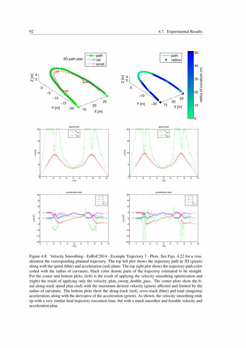
92 4.7. Experimental Results
1520
25
−20
−15
−10
−5
0
2
4
X [m]
3D path plan
Y [m]
Z [
m]
path
vel.
accel.
1520
25
−20
−10
0
24
X [m]Y [m]
Z [
m]
rad
ius o
f cu
rva
ture
(m
)
0
10
20
30
40
50path
radius
0 1 2 3 4 5 6 7 8 9 100
5
10
15
20speed plan
t [s]
v [
m/s
]
v
max
vplan
0 1 2 3 4 5 6 7 8 9 10−20
−15
−10
−5
0
5
10
15
20acceleration plan
t [s]
a [
m/s
2]
a
at
act
atotal
daat
/dt
0 1 2 3 4 5 6 7 8 9 100
5
10
15
20speed plan
t [s]
v [
m/s
]
v
max
vplan
0 1 2 3 4 5 6 7 8 9 10−20
−15
−10
−5
0
5
10
15
20acceleration plan
t [s]
a [
m/s
2]
a
at
act
atotal
daat
/dt
Figure 4.8: Velocity Smoothing - EuRoC2014 - Example Trajectory 7 - Plots. See Figs. 4.22 for a visu-alization the corresponding planned trajectory. The top left plot shows the trajectory path in 3D (green)along with the speed (blue) and acceleration (red) plans. The top right plot shows the trajectory path colorcoded with the radius of curvature, black color denote parts of the trajectory estimated to be straight.For the center and bottom plots, (left) is the result of applying the velocity smoothing optimization and(right) the result of applying only the velocity_plan_sweep_double_pass. The center plots show the fi-nal along-track speed plan (red) with the maximum desired velocity (green) affected and limited by theradius of curvature. The bottom plots show the along-track (red), cross-track (blue) and total (magenta)acceleration, along with the derivative of the acceleration (green). As shown, the velocity smoothing endsup with a very similar final trajectory execution time, but with a much smoother and feasible velocity andacceleration plan.

Chapter 4. Smooth Trajectory Planning for Multirotors 93
4.7.3.2 Comparison - Number of velocity smoothing passes - speed and acceleration plans
0 1 2 3 4 5 6 7 8 9 100
5
10
15
20speed plan
t [s]
v [m
/s]
v
max
vplan
0 1 2 3 4 5 6 7 8 9 10−20
−15
−10
−5
0
5
10
15
20acceleration plan
t [s]
a [m
/s2]
a
at
act
atotal
daat
/dt
0 1 2 3 4 5 6 7 8 9 100
5
10
15
20speed plan
t [s]
v [m
/s]
v
max
vplan
0 1 2 3 4 5 6 7 8 9 10−20
−15
−10
−5
0
5
10
15
20acceleration plan
t [s]
a [m
/s2]
a
at
act
atotal
daat
/dt
0 1 2 3 4 5 6 7 8 9 100
5
10
15
20speed plan
t [s]
v [m
/s]
v
max
vplan
0 1 2 3 4 5 6 7 8 9 10−20
−15
−10
−5
0
5
10
15
20acceleration plan
t [s]
a [m
/s2]
a
at
act
atotal
daat
/dt
0 1 2 3 4 5 6 7 8 9 100
5
10
15
20speed plan
t [s]
v [m
/s]
v
max
vplan
0 1 2 3 4 5 6 7 8 9 10−20
−15
−10
−5
0
5
10
15
20acceleration plan
t [s]
a [m
/s2]
a
at
act
atotal
daat
/dt
Figure 4.9: Velocity Smoothing - EuRoC2014 - Example Trajectory 7 - Plots. See Figs. 4.22 for avisualization the corresponding planned trajectory. Each pair of plots shows a different number of veloc-ity smoothing passes and maximum acceleration derivative, (upper left)
[1; 19 m
s3
](upper right)
[5; 15 m
s3
](down left)
[10; 11 m
s3
](down right)
[20; 9 m
s3
]. The top plots show the final along-track speed plan (red)
with the maximum desired velocity (green) affected and limited by the radius of curvature. The bot-tom plots show the along-track (red), cross-track (blue) and total (magenta) acceleration, along with thederivative of the acceleration (green). As shown, for a given set of the smoothing strength parameters{λ1,λ2,λ3}, increasing the number of reruns of the smoothing spline optimization results in smootherspeed plans, with lower maximum values for the acceleration derivative.

94 4.7. Experimental Results
4.7.3.3 Plots of trajectories, speed and acceleration plans
Figure 4.10: Trajectory Planner - EuRoC2014 - Example Trajectory 1 - RGB. The octomap is color-coded from low altitude (pink) to high altitude (clear blue). A typical planned trajectory is shown: Theoutput of the PRMStar algorithm (red) is consecutively shortened (green-blue-orange-white). The semitransparent lines show the velocity and acceleration plans.
−4
−2
0
2 −25
−20
−15
−10
−5
0
5
7
9
11
13
15
3D path plan
Y [m]
X [m]
Z [m
]
path
vel.
accel.
−4
−2
0
2 −25
−20
−15
−10
−5
5
7
9
11
13
15
Y [m]
X [m]
Z [m
]
radiu
s o
f curv
atu
re (
m)
0
5
10
15
20
25
30
35
40
45
50path
radius
0 1 2 3 4 5 6 7 80
2
4
6
8
10
12
14
16
18
20speed plan
t [s]
v [
m/s
]
vmax
vplan
0 1 2 3 4 5 6 7 8−20
−15
−10
−5
0
5
10
15
20acceleration plan
t [s]
a [
m/s
2]
a
at
act
atotal
daat
/dt
Figure 4.11: Trajectory Planner - EuRoC2014 - Example Trajectory 1 - Plots. The top left plot showsthe trajectory path in 3D (green) along with the speed (blue) and acceleration (red) plans. The bottom leftplot shows the trajectory path color coded with the radius of curvature, black color denote parts of thetrajectory estimated to be straight. The right top plot shows the final along-track speed plan (red) with themaximum desired velocity (green) affected and limited by the radius of curvature. The right bottom plotshows the along-track (red), cross-track (blue) and total (magenta) acceleration, along with the derivativeof the acceleration (green).

Chapter 4. Smooth Trajectory Planning for Multirotors 95
Figure 4.12: Trajectory Planner - EuRoC2014 - Example Trajectory 2 - RGB. The octomap is color-coded from low altitude (pink) to high altitude (clear blue). A typical planned trajectory is shown: Theoutput of the PRMStar algorithm (red) is consecutively shortened (green-blue-orange-white). The semitransparent lines show the velocity and acceleration plans.
5
10
15
20
−25
−20
−15
X [m]
3D path plan
Y [m]
Z [m
]
path
vel.
accel.
5
10
15
20
−25
−20
−15
X [m]Y [m]
Z [m
]
radiu
s o
f curv
atu
re (
m)
0
5
10
15
20
25
30
35
40
45
50path
radius
0 1 2 3 4 5 6−5
0
5
10
15
20speed plan
t [s]
v [
m/s
]
vmax
vplan
0 1 2 3 4 5 6−20
−15
−10
−5
0
5
10
15
20acceleration plan
t [s]
a [
m/s
2]
a
at
act
atotal
daat
/dt
Figure 4.13: Trajectory Planner - EuRoC2014 - Example Trajectory 2 - Plots. The top left plot showsthe trajectory path in 3D (green) along with the speed (blue) and acceleration (red) plans. The bottom leftplot shows the trajectory path color coded with the radius of curvature, black color denote parts of thetrajectory estimated to be straight. The right top plot shows the final along-track speed plan (red) with themaximum desired velocity (green) affected and limited by the radius of curvature. The right bottom plotshows the along-track (red), cross-track (blue) and total (magenta) acceleration, along with the derivativeof the acceleration (green).
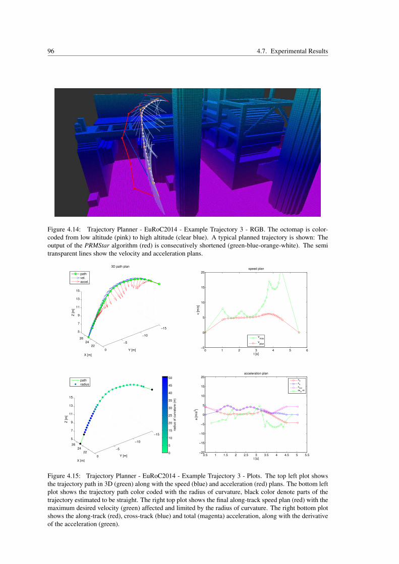
96 4.7. Experimental Results
Figure 4.14: Trajectory Planner - EuRoC2014 - Example Trajectory 3 - RGB. The octomap is color-coded from low altitude (pink) to high altitude (clear blue). A typical planned trajectory is shown: Theoutput of the PRMStar algorithm (red) is consecutively shortened (green-blue-orange-white). The semitransparent lines show the velocity and acceleration plans.
2224
26
−15
−10
−5
0
5
7
9
11
13
15
Y [m]
3D path plan
X [m]
Z [m
]
path
vel.
accel.
22
24
26
−15
−10
−5
0
5
7
9
11
13
15
Y [m]
X [m]
Z [m
]
radiu
s o
f curv
atu
re (
m)
0
5
10
15
20
25
30
35
40
45
50path
radius
0 1 2 3 4 5 6−5
0
5
10
15
20speed plan
t [s]
v [
m/s
]
vmax
vplan
0.5 1 1.5 2 2.5 3 3.5 4 4.5 5 5.5−20
−15
−10
−5
0
5
10
15
20acceleration plan
t [s]
a [
m/s
2]
a
at
act
atotal
daat
/dt
Figure 4.15: Trajectory Planner - EuRoC2014 - Example Trajectory 3 - Plots. The top left plot showsthe trajectory path in 3D (green) along with the speed (blue) and acceleration (red) plans. The bottom leftplot shows the trajectory path color coded with the radius of curvature, black color denote parts of thetrajectory estimated to be straight. The right top plot shows the final along-track speed plan (red) with themaximum desired velocity (green) affected and limited by the radius of curvature. The right bottom plotshows the along-track (red), cross-track (blue) and total (magenta) acceleration, along with the derivativeof the acceleration (green).
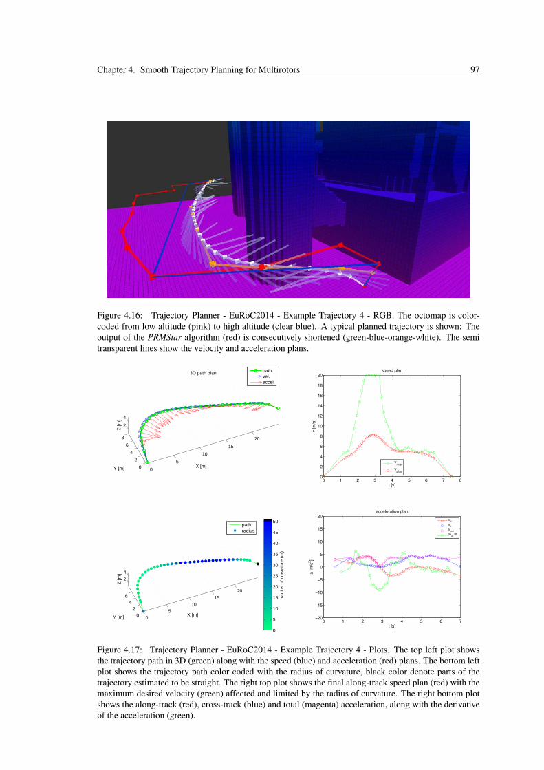
Chapter 4. Smooth Trajectory Planning for Multirotors 97
Figure 4.16: Trajectory Planner - EuRoC2014 - Example Trajectory 4 - RGB. The octomap is color-coded from low altitude (pink) to high altitude (clear blue). A typical planned trajectory is shown: Theoutput of the PRMStar algorithm (red) is consecutively shortened (green-blue-orange-white). The semitransparent lines show the velocity and acceleration plans.
0
5
10
15
20
0
2
4
6
8
2
4
3D path plan
X [m]
Y [m]
Z [m
]
path
vel.
accel.
0
5
10
15
20
0
2
4
6
2
4
X [m]
Y [m]
Z [m
]
radiu
s o
f curv
atu
re (
m)
0
5
10
15
20
25
30
35
40
45
50path
radius
0 1 2 3 4 5 6 7 80
2
4
6
8
10
12
14
16
18
20speed plan
t [s]
v [
m/s
]
vmax
vplan
0 1 2 3 4 5 6 7−20
−15
−10
−5
0
5
10
15
20acceleration plan
t [s]
a [
m/s
2]
a
at
act
atotal
daat
/dt
Figure 4.17: Trajectory Planner - EuRoC2014 - Example Trajectory 4 - Plots. The top left plot showsthe trajectory path in 3D (green) along with the speed (blue) and acceleration (red) plans. The bottom leftplot shows the trajectory path color coded with the radius of curvature, black color denote parts of thetrajectory estimated to be straight. The right top plot shows the final along-track speed plan (red) with themaximum desired velocity (green) affected and limited by the radius of curvature. The right bottom plotshows the along-track (red), cross-track (blue) and total (magenta) acceleration, along with the derivativeof the acceleration (green).

98 4.7. Experimental Results
Figure 4.18: Trajectory Planner - EuRoC2014 - Example Trajectory 5 - RGB. The octomap is color-coded from low altitude (pink) to high altitude (clear blue). A typical planned trajectory is shown: Theoutput of the PRMStar algorithm (red) is consecutively shortened (green-blue-orange-white). The semitransparent lines show the velocity and acceleration plans.
0
5
10
15
20
−15
−10
−5
0
5
5
7
9
11
13
15
X [m]
3D path plan
Y [m]
Z [
m]
path
vel.
accel.
0
5
10
15
20
−15
−10
−5
0
5
5
7
9
11
13
15
X [m]Y [m]
Z [
m]
rad
ius o
f cu
rva
ture
(m
)
0
5
10
15
20
25
30
35
40
45
50path
radius
0 1 2 3 4 5 6 7 8 90
2
4
6
8
10
12
14
16
18
20speed plan
t [s]
v [
m/s
]
vmax
vplan
0 1 2 3 4 5 6 7 8 9−20
−15
−10
−5
0
5
10
15
20acceleration plan
t [s]
a [
m/s
2]
a
at
act
atotal
daat
/dt
Figure 4.19: Trajectory Planner - EuRoC2014 - Example Trajectory 5 - Plots. The top left plot showsthe trajectory path in 3D (green) along with the speed (blue) and acceleration (red) plans. The bottom leftplot shows the trajectory path color coded with the radius of curvature, black color denote parts of thetrajectory estimated to be straight. The right top plot shows the final along-track speed plan (red) with themaximum desired velocity (green) affected and limited by the radius of curvature. The right bottom plotshows the along-track (red), cross-track (blue) and total (magenta) acceleration, along with the derivativeof the acceleration (green).
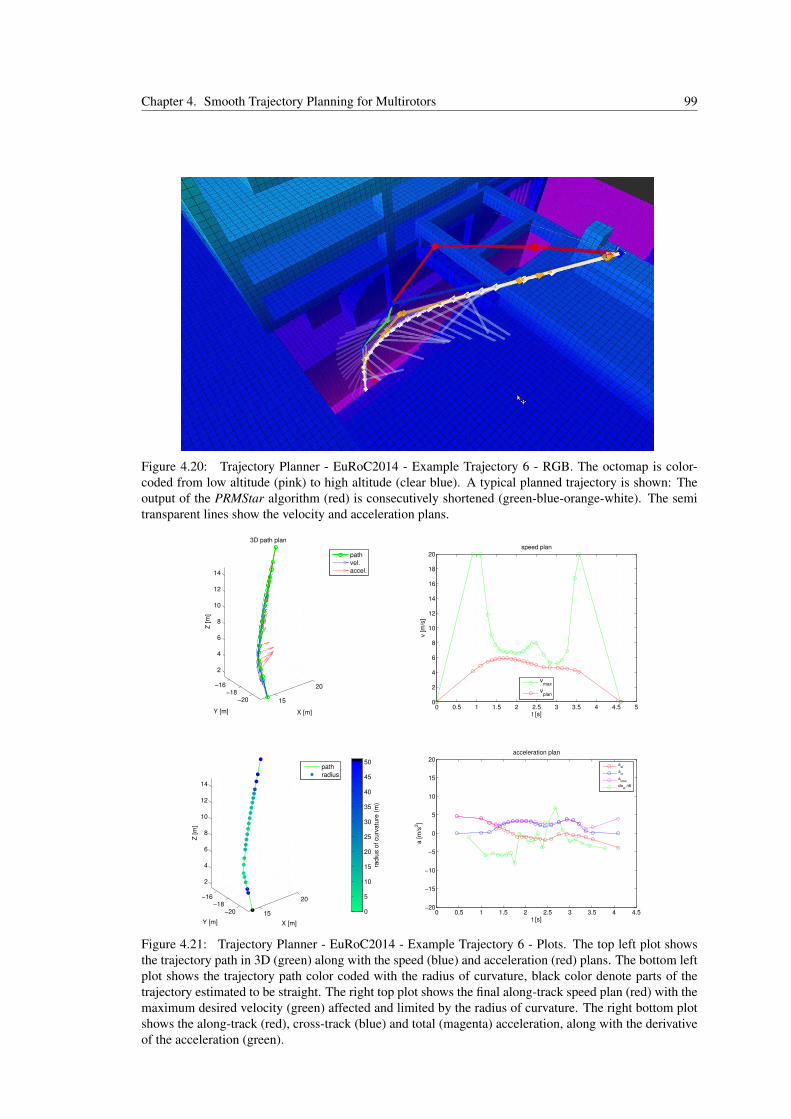
Chapter 4. Smooth Trajectory Planning for Multirotors 99
Figure 4.20: Trajectory Planner - EuRoC2014 - Example Trajectory 6 - RGB. The octomap is color-coded from low altitude (pink) to high altitude (clear blue). A typical planned trajectory is shown: Theoutput of the PRMStar algorithm (red) is consecutively shortened (green-blue-orange-white). The semitransparent lines show the velocity and acceleration plans.
15
20
−20−18
−16
2
4
6
8
10
12
14
X [m]
3D path plan
Y [m]
Z [m
]
path
vel.
accel.
15
20
−20−18
−16
2
4
6
8
10
12
14
X [m]Y [m]
Z [m
]
radiu
s o
f curv
atu
re (
m)
0
5
10
15
20
25
30
35
40
45
50path
radius
0 0.5 1 1.5 2 2.5 3 3.5 4 4.5 50
2
4
6
8
10
12
14
16
18
20speed plan
t [s]
v [m
/s]
vmax
vplan
0 0.5 1 1.5 2 2.5 3 3.5 4 4.5−20
−15
−10
−5
0
5
10
15
20acceleration plan
t [s]
a [m
/s2]
a
at
act
atotal
daat
/dt
Figure 4.21: Trajectory Planner - EuRoC2014 - Example Trajectory 6 - Plots. The top left plot showsthe trajectory path in 3D (green) along with the speed (blue) and acceleration (red) plans. The bottom leftplot shows the trajectory path color coded with the radius of curvature, black color denote parts of thetrajectory estimated to be straight. The right top plot shows the final along-track speed plan (red) with themaximum desired velocity (green) affected and limited by the radius of curvature. The right bottom plotshows the along-track (red), cross-track (blue) and total (magenta) acceleration, along with the derivativeof the acceleration (green).

100 4.7. Experimental Results
Figure 4.22: Trajectory Planner - EuRoC2014 - Example Trajectory 7 - RGB. The octomap is color-coded from low altitude (pink) to high altitude (clear blue). A typical planned trajectory is shown: Theoutput of the PRMStar algorithm (red) is consecutively shortened (green-blue-orange-white). The semitransparent lines show the velocity and acceleration plans.
15
20
25
−20
−15
−10
−5
0
2
4
X [m]
3D path plan
Y [m]
Z [m
]
path
vel.
accel.
15
20
25
−20
−15
−10
−5
0
2
4
X [m]
Y [m]
Z [m
]
radiu
s o
f curv
atu
re (
m)
0
5
10
15
20
25
30
35
40
45
50path
radius
0 1 2 3 4 5 6 7 8 9 100
5
10
15
20speed plan
t [s]
v [m
/s]
v
max
vplan
0 1 2 3 4 5 6 7 8 9 10−20
−15
−10
−5
0
5
10
15
20acceleration plan
t [s]
a [m
/s2]
a
at
act
atotal
daat
/dt
Figure 4.23: Trajectory Planner - EuRoC2014 - Example Trajectory 7 - Plots. The top left plot showsthe trajectory path in 3D (green) along with the speed (blue) and acceleration (red) plans. The bottom leftplot shows the trajectory path color coded with the radius of curvature, black color denote parts of thetrajectory estimated to be straight. The right top plot shows the final along-track speed plan (red) with themaximum desired velocity (green) affected and limited by the radius of curvature. The right bottom plotshows the along-track (red), cross-track (blue) and total (magenta) acceleration, along with the derivativeof the acceleration (green).

Chapter 4. Smooth Trajectory Planning for Multirotors 101
Figure 4.24: Trajectory Planner - EuRoC2014 - Example Trajectory 8 - RGB. The octomap is color-coded from low altitude (pink) to high altitude (clear blue). A typical planned trajectory is shown: Theoutput of the PRMStar algorithm (red) is consecutively shortened (green-blue-orange-white). The semitransparent lines show the velocity and acceleration plans.
5
10
15
20
25
−20
−15
−10
5
7
9
11
13
15
X [m]
3D path plan
Y [m]
Z [m
]
path
vel.
accel.
5
10
15
20
25
−20
−15
−10
5
7
9
11
13
15
X [m]Y [m]
Z [m
]
radiu
s o
f curv
atu
re (
m)
0
5
10
15
20
25
30
35
40
45
50path
radius
0 1 2 3 4 5 6 7 80
2
4
6
8
10
12
14
16
18
20speed plan
t [s]
v [
m/s
]
vmax
vplan
0 1 2 3 4 5 6 7 8−20
−15
−10
−5
0
5
10
15
20acceleration plan
t [s]
a [
m/s
2]
a
at
act
atotal
daat
/dt
Figure 4.25: Trajectory Planner - EuRoC2014 - Example Trajectory 8 - Plots. The top left plot showsthe trajectory path in 3D (green) along with the speed (blue) and acceleration (red) plans. The bottom leftplot shows the trajectory path color coded with the radius of curvature, black color denote parts of thetrajectory estimated to be straight. The right top plot shows the final along-track speed plan (red) with themaximum desired velocity (green) affected and limited by the radius of curvature. The right bottom plotshows the along-track (red), cross-track (blue) and total (magenta) acceleration, along with the derivativeof the acceleration (green).

102 4.7. Experimental Results
Figure 4.26: Trajectory Planner - EuRoC2014 - Example Trajectory 9 - RGB. The octomap is color-coded from low altitude (pink) to high altitude (clear blue). A typical planned trajectory is shown: Theoutput of the PRMStar algorithm (red) is consecutively shortened (green-blue-orange-white). The semitransparent lines show the velocity and acceleration plans.
02
4−6
−4−2
0
5
7
9
11
13
15
X [m]
3D path plan
Y [m]
Z [m
]
path
vel.
accel.
02
4−5
0
2
4
6
8
10
12
14
16
X [m]Y [m]
Z [m
]
radiu
s o
f curv
atu
re (
m)
0
5
10
15
20
25
30
35
40
45
50path
radius
0 1 2 3 4 5 6 7−5
0
5
10
15
20speed plan
t [s]
v [m
/s]
vmax
vplan
0 1 2 3 4 5 6−20
−15
−10
−5
0
5
10
15
20acceleration plan
t [s]
a [m
/s2]
a
at
act
atotal
daat
/dt
Figure 4.27: Trajectory Planner - EuRoC2014 - Example Trajectory 9 - Plots. The top left plot showsthe trajectory path in 3D (green) along with the speed (blue) and acceleration (red) plans. The bottom leftplot shows the trajectory path color coded with the radius of curvature, black color denote parts of thetrajectory estimated to be straight. The right top plot shows the final along-track speed plan (red) with themaximum desired velocity (green) affected and limited by the radius of curvature. The right bottom plotshows the along-track (red), cross-track (blue) and total (magenta) acceleration, along with the derivativeof the acceleration (green).

Chapter 4. Smooth Trajectory Planning for Multirotors 103
4.7.4 Results in 2016 DJI Developer Challenge - Experimental FlightsThe trajectory planner used in the participation of the “Graz Griffins” to the 2016 DJI Developer
Challenge utilized the PRM* for the second deliverable and the RRT* later on. The main differencebetween using one or the other in terms of usability is that using the RRT* allows to work with dynamicenvironments. The trajectories shown in this section where generated using the PRM* algorithm.
The controller utilized in this challenge was inspired by the one used by the team in the EuRoC2014and it was also developed by D. Muschick for the “Graz Griffins” team. In this case, a third order splineis fitted to the provided trajectory path and times of passage. The following performance parameters,see Table 4.2, correspond to the video uploaded here20. In this experiment the octomap size is around200×55 m, and the octomap resolution used by the planner is 1 m (which does not match what is shownin the figures of the next subsection, that show an octomap of resolution 0.50 m). For the trajectoryplanner, the maximum speed was set to 4.0 m/s and the acceleration to 0.15 g = 1.47 m/s2 All thecontrol architecture is executed on-board the drone except for a user interface to command the drone onwhere to fly next.
path length [m] UI+plan execution total time [s] max speed[m/s]
77.24 2.52 26.57 / 25.47 29.09 / 27.99 4.0043.53 1.66 15.67 / 14.93 17.33 / 16.59 4.0044.96 2.09 15.58 / 14.89 17.67 / 16.98 4.0080.52 2.88 24.68 / 23.78 27.56 / 26.66 4.0061.56 2.29 20.63 / 19.77 22.91 / 22.06 « averages
Table 4.2: Trajectory planning and control performance - 2016 DJI Developer Challenge. All the valuesshown in the table are derived from a datalog of the flight, considering the times at which ROS messageswere published. All the control architecture is executed on-board the drone except for a user interface tocommand the drone on where to fly next. The UI+plan time corresponds to the whole trajectory generationtime plus the time that it took between clicking on the next target point on the User Interface (ROS Rviz)to receiving the goal point in the drone through WiFi. The execution time is the time that it took thecontroller to perform the commanded trajectory, where the left column shows the actual execution timeand the right expected or planned execution time. And the total time is the sum of both. The averageachieved navigation speed was: [(real) / (planned)] 2.98 / 3.11 m/s.
In the next subsection trajectories resulting from the presented trajectory planning and subsequentspeed and acceleration planning algorithms are shown. The trajectories are the ones utilized during theexecution of the same video20. These plots show the following:
• The calculated obstacle-free smooth trajectories
• The calculated speed and acceleration plans, and the corresponding times-of-passage plan.
• The estimated radius of curvature at each point of the trajectory path. Note how the radius ofcurvature affects the maximum velocity of the speed plan before, inside and after curves.
• Note how the acceleration and speed plans are correctly limited to the desired values, and how thederivative of the acceleration remains reasonable.
20 https://youtu.be/9DXzIGKKqbU

104 4.7. Experimental Results
4.7.4.1 Plots of trajectories, speed and acceleration plans
Figure 4.28: Trajectory Planner - 2016 DJI Developer Challenge - Example Trajectory 1 - RGB. Theoctomap is color-coded from low altitude (pink) to high altitude (green). A typical planned trajectory isshown in white, and the semi transparent lines show the velocity and acceleration plans.
−30
−20
−10
0
−20
−10
0
10
20
30
02
X [m]
3D path plan
Y [m]
Z [
m]
path
vel.
accel.
−20
−10
0
−20
−10
0
10
20
02
X [m]
Y [m]
Z [
m]
rad
ius o
f cu
rva
ture
(m
)
0
5
10
15
20
25
30
35
40
45
50path
radius
0 5 10 15 20 250
0.5
1
1.5
2
2.5
3
3.5
4speed plan
t [s]
v [
m/s
]
vmax
vplan
0 5 10 15 20 25−2
−1.5
−1
−0.5
0
0.5
1
1.5
2acceleration plan
t [s]
a [
m/s
2]
aat
act
atotal
daat
/dt
Figure 4.29: Trajectory Planner - 2016 DJI Developer Challenge - Example Trajectory 1 - Plots. Thetop left plot shows the trajectory path in 3D (green) along with the speed (blue) and acceleration (red)plans. The bottom left plot shows the trajectory path color coded with the radius of curvature, black colordenote parts of the trajectory estimated to be straight. The right top plot shows the final along-track speedplan (red) with the maximum desired velocity (green) affected and limited by the radius of curvature. Theright bottom plot shows the along-track (red), cross-track (blue) and total (magenta) acceleration, alongwith the derivative of the acceleration (green).

Chapter 4. Smooth Trajectory Planning for Multirotors 105
Figure 4.30: Trajectory Planner - 2016 DJI Developer Challenge - Example Trajectory 2 - RGB. Theoctomap is color-coded from low altitude (pink) to high altitude (green). A typical planned trajectory isshown in white, and the semi transparent lines show the velocity and acceleration plans.
−45
−40
−35
−30
−25
30
35
40
45
50
55
0
2
X [m]
3D path plan
Y [m]
Z [m
]
path
vel.
accel.
−40
−35
−30
30
35
40
45
50
55
0
2
X [m]
Y [m]
Z [m
]
radiu
s o
f curv
atu
re (
m)
0
5
10
15
20
25
30
35
40
45
50path
radius
0 5 10 150
0.5
1
1.5
2
2.5
3
3.5
4speed plan
t [s]
v [
m/s
]
vmax
vplan
0 2 4 6 8 10 12 14−2
−1.5
−1
−0.5
0
0.5
1
1.5
2acceleration plan
t [s]
a [
m/s
2]
aat
act
atotal
daat
/dt
Figure 4.31: Trajectory Planner - 2016 DJI Developer Challenge - Example Trajectory 2 - Plots. Thetop left plot shows the trajectory path in 3D (green) along with the speed (blue) and acceleration (red)plans. The bottom left plot shows the trajectory path color coded with the radius of curvature, black colordenote parts of the trajectory estimated to be straight. The right top plot shows the final along-track speedplan (red) with the maximum desired velocity (green) affected and limited by the radius of curvature. Theright bottom plot shows the along-track (red), cross-track (blue) and total (magenta) acceleration, alongwith the derivative of the acceleration (green).

106 4.7. Experimental Results
Figure 4.32: Trajectory Planner - 2016 DJI Developer Challenge - Example Trajectory 3 - RGB. Theoctomap is color-coded from low altitude (pink) to high altitude (green). A typical planned trajectory isshown in white, and the semi transparent lines show the velocity and acceleration plans.
−40
−35
−30
−25
25
30
35
40
45
50
55
0
2
X [m]
3D path plan
Y [m]
Z [
m]
path
vel.
accel.
−40
−35
−30
30
35
40
45
50
55
0
2
X [m]
Y [m]
Z [
m]
rad
ius o
f cu
rva
ture
(m
)
0
5
10
15
20
25
30
35
40
45
50path
radius
0 5 10 150
0.5
1
1.5
2
2.5
3
3.5
4speed plan
t [s]
v [
m/s
]
vmax
vplan
0 2 4 6 8 10 12 14−2
−1.5
−1
−0.5
0
0.5
1
1.5
2acceleration plan
t [s]
a [m
/s2]
aat
act
atotal
daat
/dt
Figure 4.33: Trajectory Planner - 2016 DJI Developer Challenge - Example Trajectory 3 - Plots. Thetop left plot shows the trajectory path in 3D (green) along with the speed (blue) and acceleration (red)plans. The bottom left plot shows the trajectory path color coded with the radius of curvature, black colordenote parts of the trajectory estimated to be straight. The right top plot shows the final along-track speedplan (red) with the maximum desired velocity (green) affected and limited by the radius of curvature. Theright bottom plot shows the along-track (red), cross-track (blue) and total (magenta) acceleration, alongwith the derivative of the acceleration (green).

Chapter 4. Smooth Trajectory Planning for Multirotors 107
Figure 4.34: Trajectory Planner - 2016 DJI Developer Challenge - Example Trajectory 4 - RGB. Theoctomap is color-coded from low altitude (pink) to high altitude (green). A typical planned trajectory isshown in white, and the semi transparent lines show the velocity and acceleration plans.
−20
−10
0
−40
−30
−20
−10
0
10
20
02
X [m]
3D path plan
Y [m]
Z [m
]
path
vel.
accel.
−20
−10
0
−30
−20
−10
0
10
20
02
X [m]
Y [m]
Z [m
]
radiu
s o
f curv
atu
re (
m)
0
5
10
15
20
25
30
35
40
45
50path
radius
0 5 10 15 20 250
0.5
1
1.5
2
2.5
3
3.5
4speed plan
t [s]
v [
m/s
]
vmax
vplan
0 5 10 15 20 25−2
−1.5
−1
−0.5
0
0.5
1
1.5
2acceleration plan
t [s]
a [
m/s
2]
aat
act
atotal
daat
/dt
Figure 4.35: Trajectory Planner - 2016 DJI Developer Challenge - Example Trajectory 4 - Plots. Thetop left plot shows the trajectory path in 3D (green) along with the speed (blue) and acceleration (red)plans. The bottom left plot shows the trajectory path color coded with the radius of curvature, black colordenote parts of the trajectory estimated to be straight. The right top plot shows the final along-track speedplan (red) with the maximum desired velocity (green) affected and limited by the radius of curvature. Theright bottom plot shows the along-track (red), cross-track (blue) and total (magenta) acceleration, alongwith the derivative of the acceleration (green).

108 4.8. Future Work
4.8 Future WorkIn the area of trajectory planning, the navigation control performs better when following smooth
trajectories, allowing faster motion. Additionally, less computer intensive trajectory generation algorithmsallow the drone to make rapid decisions while navigating in cluttered environments or while performingtime critical operations. Since robots can move and affect which data is going to be gathered for themapping of the environment, another innovative research trend is acknowledging the inter-dependencein robotics of exploration, obstacle mapping and trajectory planning. For instance, the development oftrajectory planning strategies that utilize obstacle maps that encode uncertainty. There is also a trend tocombine image processing and motion planning where these two tasks are not separated in modules butrather solved together by means of deep learning. Some works have already shown promising results inobject grasping and door opening by robot arm manipulators, but similar techniques are still to be appliedto drones.
4.9 ConclusionsIn this chapter, a novel trajectory planner for multirotors has been presented. The main purpose of
this planner is to enable outdoors flight in relatively cluttered environments. As shown in the results theplanner is able to deliver smooth safe trajectories when flying near buildings and other obstacles. Thefollowing features of the planner have been demonstrated:
• The algorithm is lightweight enough that it can be executed on the on-board computer of the drone.
• The algorithm has been tested experimentally on maps obtained using an on-board real-time capableComputer Vision photogrammetry method.
• It utilizes the Octomap obstacle map representation, which is commonly used in robotics. Theutilization of a distance map, to all present obstacles, is leveraged for the calculation of obstacle-free smooth trajectories.
• A feasible speed, acceleration and time-of-passage plans are delivered along with the trajectorypath. The algorithm enforces the set maximum desired speed and acceleration. The speed plan isthe result of a refinement to bound the jerk, i. e. the derivative of the acceleration, of the trajectoryso that the drone can fly through it using smoother rotations. The speed plan refinement has beenshown to improve the result in terms of lower acceleration derivative values and of smoother speedand acceleration plans.
• Although other modules would be needed to decide the exact navigation objectives of the drone,using this planner we have shown that it is feasible to deploy drones in unknown outdoors envi-ronments, by leveraging the good qualities of maps obtained using state of the art photogrammetrymapping methods.
The main publications related to this chapter are:
• J. Pestana, M. Maurer, D. Muschick, D. Adlakha, H. Bischof, F. Fraundorfer, “Package DeliveryExperiments with a Camera Drone”. In Austrian Robotics Workshop 2017, OAGM/AAPR2017 jointWorkshop. To be published.
• J. Pestana and F. Fraundorfer, “Vision based safe navigation for search and rescue drones” inthe IEEE/RSJ IROS2016 Workshop “Vision-Based High Speed Autonomous Navigation of UAVs”.[No Proceedings] https://www.seas.upenn.edu/~loiannog/workshopIROS2016uav/
• J. Pestana, R. Prettenthaler, T. Holzmann, D. Muschick, C. Mostegel, F. Fraundorfer, H. Bischof“Graz Griffins' Solution to the European Robotics Challenges 2014”. In Austrian Robotics Work-shop 2015, ARW2015.
• T Holzmann, R Prettenthaler, J. Pestana, D Muschick, G Graber, C Mostegel, F Fraundorfer, HBischof “Performance Evaluation of Vision-Based Algorithms for MAVs”. In Austrian Associationfor Pattern Recognition Conference 2015, OAGM2015.

Chapter 4. Smooth Trajectory Planning for Multirotors 109
• The author of this thesis is currently working in two publications based on works related to eitherthe presented trajectory planner or the 2016 DJI Developer Challenge.
The presented trajectory planner and related speed planning algorithm has been used by the ICG - TUGraz in its participation in two international MAV competitions as the team named the “Graz Griffins”:
• 2016 DJI Developer Challenge (DJIC 2016)21: the competition recreated a drone Search and Res-cue scenario. The “Graz Griffins” team qualified through successive rounds, from the initial ≈140teams, to be part of the last 10 teams showing their solution experimentally in the finals. The teamshowed a very innovative solution using on-board mapping based on photogrammetry algorithms.The on-board calculated map is converted to an obstacle-map that can be used by the presentedplanner to deliver trajectories that are then executed by the controller, all in the same flight andwithout requiring any off-board computation.
• European Robotics Challenge (EuRoC 2014)22: The “Graz Griffins” took part in the SimulationContest of the European Robotics Challenge (EuRoC) - Challenge 3. The developed fast real-timetrajectory and speed planner enabled reliable obstacle avoidance and very fast trajectory executionby the simulated quadrotor that replicated the capabilities of an Asctec Firefly MAV. The developedplanner contributed to the 6th position of the “Graz Griffins” out of 21 teams, which included worldrenowned European universities and laboratories. This fact enabled the team to present a proposalin collaboration with a company to the next stage of the challenge.
The works related to the 2016 DJI Developer Challenge have been presented or showcased in twopublic events so far:
• An experimental fully autonomous package delivery flight demonstration made by theICG - TU Graz23in collaboration with the company SFL Technologies as part of the roll-out of theirbrand new electric vehicle, the ELI. The roll-out of this vehicle and the autonomous flight demohave been described by two Austrian newspapers: Mein Bezirk24 and Kleine Zeitung25.November 2016
• A public presentation, with no experimental flights, named Intelligent Search and Rescue Dronein the world renowned Ars Electronica Festival 2016 - DroneLab - FutureLab26. This festivalshows modern artwork that utilizes technology as a medium of expression and tries to deliver anoutstanding and open view of current technology developments to its public.September 8-12, 2016
21DJIC 2016 video playlist: http://bit.ly/2faublQ22EuRoC 2014 trajectory flight video: http://bit.ly/2cQnO6I23Fully autonomous package delivery flight demonstration: https://youtu.be/bxM6dls2wuo24ELI roll-out - Mein Bezirk - http://bit.ly/2hott8t25ELI roll-out - Kleine Zeitung - http://bit.ly/2it6N2P26Ars Electronica Festival 2016 - DroneLab: http://www.aec.at/radicalatoms/en/ars-electronica-dronelab/

110 4.10. Chapter Bibliography
4.10 Chapter BibliographyCowling, I. D., Yakimenko, O. A., Whidborne, J. F., and Cooke, A. K. (2010). “Direct method based
control system for an autonomous quadrotor”. Journal of Intelligent & Robotic Systems 60.2, pp. 285–316 (cit. on p. 70).
Dijkstra, E. W. (1959). “A note on two problems in connexion with graphs”. Numerische mathematik 1.1,pp. 269–271 (cit. on pp. 76, 77).
Dunbar, N. and Franz, R. (2003). “Online control customization via optimization, based control”.Software-Enabled Control: Information Technology for Dynamical Systems, p. 149 (cit. on p. 70).
Fliess, M., Lévine, J., Martin, P., and Rouchon, P. (1995). “Flatness and defect of non-linear systems: in-troductory theory and examples”. International journal of control 61.6, pp. 1327–1361 (cit. on p. 70).
Fritsch, O., De Monte, P., Buhl, M., and Lohmann, B. (2012). “Quasi-static feedback linearization forthe translational dynamics of a quadrotor helicopter”. In: American Control Conference (ACC), 2012.IEEE, pp. 125–130 (cit. on pp. 70, 74).
Furrer, F., Burri, M., Achtelik, M., and Siegwart, R. (2016). “RotorS-A Modular Gazebo MAV SimulatorFramework”. In: Robot Operating System (ROS). Springer, pp. 595–625 (cit. on p. 89).
Hofer, M., Maurer, M., and Bischof, H. (2016). “Efficient 3D scene abstraction using line segments”.Computer Vision and Image Understanding (cit. on p. 72).
Hoffmann, Gabriel M, Waslander, Steven L, and Tomlin, Claire J (2008). “Quadrotor Helicopter Trajec-tory Tracking Control”. Electrical Engineering (2008), pp. 1–14 (cit. on pp. 81, 82).
Holzmann, T., Prettenthaler, R., Pestana, J., Muschick, D., Graber, G., Mostegel, C., Fraundorfer, F., andBischof, H. (2015). “Performance Evaluation of Vision-Based Algorithms for MAVs”. arXiv preprintarXiv:1505.02247 (cit. on p. 90).
Hoppe, C., Klopschitz, M., Donoser, M., and Bischof, H. (2013). “Incremental Surface Extraction fromSparse Structure-from-Motion Point Clouds.” In: BMVC, pp. 94–1 (cit. on p. 73).
Hoppe, C., Klopschitz, M., Rumpler, M., Wendel, A., Kluckner, S., Bischof, H., and Reitmayr, G. (2012).“Online Feedback for Structure-from-Motion Image Acquisition.” In: BMVC. Vol. 2, p. 6 (cit. onp. 72).
Hornung, A., Wurm, K. M., Bennewitz, M., Stachniss, C., and Burgard, W. (2013). “OctoMap: An effi-cient probabilistic 3D mapping framework based on octrees”. Autonomous Robots 34.3, pp. 189–206(cit. on pp. 70, 71, 73–76).
James, G., Witten, D., Hastie, T., and Tibshirani, R. (2013). An introduction to statistical learning. Vol. 6.Springer (cit. on p. 84).
Karaman, S. and Frazzoli, E. (2011). “Sampling-based algorithms for optimal motion planning”. Theinternational journal of robotics research 30.7, pp. 846–894 (cit. on pp. 70, 74, 77, 78).
Kavraki, L. E., Svestka, P., Latombe, J.-C., and Overmars, M. H. (1996). “Probabilistic roadmaps for pathplanning in high-dimensional configuration spaces”. IEEE transactions on Robotics and Automation12.4, pp. 566–580 (cit. on pp. 70, 71, 74, 76).
Kneip, L., Scaramuzza, D., and Siegwart, R. (2011). “A novel parametrization of the perspective-three-point problem for a direct computation of absolute camera position and orientation”. In: ComputerVision and Pattern Recognition (CVPR), 2011 IEEE Conference on. IEEE, pp. 2969–2976 (cit. onp. 72).
Labatut, P., Pons, J.-P., and Keriven, R. (2007). “Efficient multi-view reconstruction of large-scale scenesusing interest points, delaunay triangulation and graph cuts”. In: 2007 IEEE 11th international con-ference on computer vision. IEEE, pp. 1–8 (cit. on p. 73).
Lau, B., Sprunk, C., and Burgard, W. (2013). “Efficient grid-based spatial representations for robot navi-gation in dynamic environments”. Elsevier RAS2013 (cit. on pp. 70, 71, 74, 76).
LaValle, S. M. (1998). “Rapidly-Exploring Random Trees: A New Tool for Path Planning” (cit. on pp. 70,71, 74, 77).
LaValle, S. M. and Kuffner, J. J. (2001). “Randomized kinodynamic planning”. The International Journalof Robotics Research 20.5, pp. 378–400 (cit. on p. 74).
Lowe, D. G. (2004). “Distinctive image features from scale-invariant keypoints”. International journal ofcomputer vision 60.2, pp. 91–110 (cit. on p. 72).
Mellinger, D. and Kumar, V. (2011). “Minimum snap trajectory generation and control for quadrotors”.In: Robotics and Automation (ICRA), 2011 IEEE International Conference on. IEEE, pp. 2520–2525(cit. on pp. 70, 74).

Chapter 4. Smooth Trajectory Planning for Multirotors 111
Meyer, J., Sendobry, A., Kohlbrecher, S., Klingauf, U., and Stryk, O. von (2012). “Comprehensive sim-ulation of quadrotor uavs using ros and gazebo”. In: Simulation, Modeling, and Programming forAutonomous Robots. Springer, pp. 400–411 (cit. on p. 89).
Murray, R. M., Rathinam, M., and Sluis, W. (1995). “Differential flatness of mechanical control systems:A catalog of prototype systems”. In: ASME International Mechanical Engineering Congress and Ex-position. Citeseer (cit. on p. 70).
Pestana, J., Prettenthaler, R., Holzmann, T., Muschick, D., Mostengel, C., Fraundorfer, F., and Bischof, H.(2015). “Graz griffins’ solution to the european robotics challenges 2014”. In: Proceedings of AustrianRobotics Workshop 2015, pp. 11–12 (cit. on pp. 88, 90).
Richter, Charles, Bry, Adam, and Roy, Nicholas (2013). “Polynomial trajectory planning for aggressivequadrotor flight in dense indoor environments”. In: Proceedings of the International Symposium onRobotics Research (ISRR) (cit. on p. 70).
Richter, C., Bry, A., and Roy, N. (2013). “Polynomial trajectory planning for quadrotor flight”. In: Inter-national Conference on Robotics and Automation (cit. on pp. 70, 71).
Rumpler, M., Tscharf, A., Mostegel, C., Daftry, S., Hoppe, C., Prettenthaler, R., Fraundorfer, F., Mayer,G., and Bischof, H. (2016). “Evaluations on multi-scale camera networks for precise and geo-accuratereconstructions from aerial and terrestrial images with user guidance”. Computer Vision and ImageUnderstanding (cit. on p. 73).
Shah, S., Dey, D., Lovett, C., and Kapoor, A. (2017). Aerial Informatics and Robotics Platform. Tech. rep.MSR-TR-2017-9. Microsoft Research (cit. on p. 89).
Sucan, I. A., Moll, M., and Kavraki, L. E. (2012). “The Open Motion Planning Library”. IEEE Robotics& Automation Magazine (cit. on pp. 70, 71, 77, 78).
Triggs, B., McLauchlan, P. F., Hartley, R. I., and Fitzgibbon, A. W. (1999). “Bundle adjustment - a modernsynthesis”. In: International workshop on vision algorithms. Springer, pp. 298–372 (cit. on pp. 84, 85).
Van Nieuwstadt, M. J. and Murray, R. M. (1998). “Real-time trajectory generation for differentially flatsystems”. International Journal of Robust and Nonlinear Control 8.11, pp. 995–1020 (cit. on p. 70).
Yanmaz, E., Hayat, S., Scherer, J., and Bettstetter, C. (2014). “Experimental performance analysis of two-hop aerial 802.11 networks”. In: 2014 IEEE Wireless Communications and Networking Conference(WCNC). IEEE, pp. 3118–3123 (cit. on p. 76).

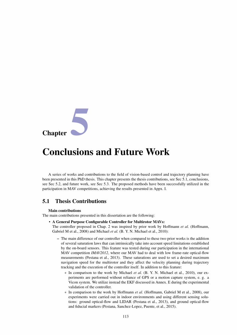
Chapter 5Conclusions and Future Work
A series of works and contributions to the field of vision-based control and trajectory planning havebeen presented in this PhD thesis. This chapter presents the thesis contributions, see Sec 5.1, conclusions,see Sec 5.2, and future work, see Sec 5.3. The proposed methods have been successfully utilized in theparticipation in MAV competitions, achieving the results presented in Appx. I.
5.1 Thesis ContributionsMain contributions
The main contributions presented in this dissertation are the following:
• A General Purpose Configurable Controller for Multirotor MAVs:The controller proposed in Chap. 2 was inspired by prior work by Hoffmann et al. (Hoffmann,Gabriel M et al., 2008) and Michael et al. (B. Y. N. Michael et al., 2010):
– The main difference of our controller when compared to these two prior works is the additionof several saturation laws that can intrinsically take into account speed limitations establishedby the on-board sensors. This feature was tested during our participation in the internationalMAV competition IMAV2012, where our MAV had to deal with low frame-rate optical-flowmeasurements (Pestana et al., 2013). These saturations are used to set a desired maximumnavigation speed for the multirotor and they affect the velocity planning during trajectorytracking and the execution of the controller itself. In addition to this feature:
* In comparison to the work by Michael et al. (B. Y. N. Michael et al., 2010), our ex-periments are performed without reliance of GPS or a motion capture system, e. g. aVicon system. We utilize instead the EKF discussed in Annex. E during the experimentalvalidation of the controller.
* In comparison to the work by Hoffmann et al. (Hoffmann, Gabriel M et al., 2008), ourexperiments were carried out in indoor environments and using different sensing solu-tions: ground optical-flow and LIDAR (Pestana et al., 2013), and ground optical-flowand fiducial markers (Pestana, Sanchez-Lopez, Puente, et al., 2015).
113
114 5.1. Thesis Contributions
– This feature of the presented controller is quite advantageous, considering that some odometryestimation algorithms may fail to deliver estimates when navigating at inadequate velocities.For instance, in vision-based odometry estimation it becomes increasingly difficult to matchimage patches or features in subsequent images, due to a lack of overlap between them, thus, inpractice, setting a maximum navigation velocity. The controller architecture proposed in thischapter under normal working conditions, e.g. within the sensors and actuators limits and inabsence of strong enough wind and wind-gusts, is able to ensure that the trajectory is executedat an optimum speed for the on-board sensors to work properly. The actual acceptable windspeed depends on the maximum speed that can be sensed by the utilized sensing algorithm.By adopting a conservative approach, in practice, the acceptable wind speed is set lower thanthe sensor limits.
– An additional usage of the speed saturations proposed in the controller architecture and inthe speed planning step is to simplify the flight rules of decentralized multi-robot navigation,as showcased in Sec. 2.4.4. This particular use of the speed saturations was utilized by theCVG_UPM during its participation in the IMAV 2013 competition.
– The presented controller has been successfully utilized as part of an autonomous flight archi-tecture in several international MAV competitions, showcasing its tested reliable implementa-tion, and its code has been released as open-source in github.
• Visual Servoing of Arbitrary Objects for Multirotors:In Chap. 3, a novel visual based object tracking and following architecture for multirotor vehiclesis presented. The contributions of this work are two-fold:
– First, it has been demonstrated that current tracking algorithms, such as OpenTLD, can reli-ably work on a fixed camera multirotor vehicle to feedback an Image Based Visual Servoing(IBVS) controller, even during high velocity autonomous navigation.
– Second, our architecture has been able to follow a large variety of unmarked targets of differentsizes and from a wide range of distances. Moreover, the algorithm is validated using a low-cost platform, the Parrot AR Drone 2.0, in outdoor conditions while tracking and followingpeople. The system has successfully and repeatedly handled occlusion events and tracked fastmoving targets, such as a person running, showing the robustness of our system against winddisturbances and illumination changes.
The main features of our architecture that made it unique at the time of the publication of our worksare:
– Our system is able to follow and stabilize itself and it is able to track a large variety of differentobjects.
– Additionally, safety is assured even when the wireless connection is suddenly degraded, thetracking is lost or the target is occluded. This is achieved by using a multirotor platform thatcan attain on-board autonomous hovering by means of floor optical flow based odometry. Theexperimental work was performed using an AR Drone 2.0, and the algorithms where run onan off-board laptop computer via a WiFi link.
– Our system has been able to repeatedly perform object following tasks for long periods oftime of up to 7 minutes (see the related videos), and fully depleting the UAV battery, after theuser is experienced enough to understand the capabilities of our object following solution.
– Our system has been able to perform visual servoing with targets of varying size, from aquarter to more than ten times the tunned target size, at varying distances from 1-2 m to 10-15 m of distance from the target, and it has has achieved person following at speeds up to2.5-3.0 m/s for a period of 45 seconds.
– The reliability of our system has been demonstrated in live demos: several performed by theCVG, at the SSRR2013 conference and with the ICG - TU Graz.
• Smooth Trajectory Planning for Multirotors:In Chap. 4, a novel trajectory planner for multirotor drones has been presented. The main purposeof this planner is to enable outdoors flight in relatively cluttered environments. As shown in the

Chapter 5. Conclusions and Future Work 115
results the planner is able to deliver smooth safe trajectories when flying near buildings and otherobstacles. The following features of the planner have been demonstrated:
– The algorithm is lightweight enough that it can be executed on the on-board computer of thedrone.
– The algorithm has been tested experimentally on maps obtained using an on-board real-timecapable Computer Vision photogrammetry method.
– It utilizes the Octomap obstacle map representation, which is commonly used in robotics.The utilization of a distance map, to all present obstacles, is leveraged for the calculation ofobstacle-free smooth trajectories.
– A feasible speed, acceleration and time-of-passage plans are delivered along with the trajec-tory path. The algorithm enforces the set maximum desired speed and acceleration. The speedplan is the result of a refinement to bound the jerk, i. e. the derivative of the acceleration, ofthe trajectory so that the drone can fly through it using smoother rotations. The speed plan re-finement has been shown to improve the result in terms of lower acceleration derivative valuesand of smoother speed and acceleration plans.
– Although other modules would be needed to decide the exact navigation objectives of thedrone, using this planner we have shown that it is feasible to deploy drones in unknown out-doors environments, by leveraging the good qualities of maps obtained using state of the artphotogrammetry mapping methods.
Main scientific publications:The main scientific publications derived from the work realized during the realization of this PhD Thesisare the following:
• A General Purpose Configurable Controller for Multirotor MAVsThe main publications related to control architecture proposed in Chap. 2 are:
– J. Pestana, J. L. Sanchez-Lopez, P. de la Puente, A. Carrio, P. Campoy. “A Vision-basedQuadrotor Multi-robot Solution for the Indoor Autonomy Challenge of the 2013 InternationalMicro Air Vehicle Competition”. In Journal of Intelligent and Robotic Systems, JINT2015.Springer Netherlands.
– J. Pestana, I. Mellado-Bataller, C. Fu, J. L. Sanchez-Lopez, I. F. Mondragon, P. Campoy. “AGeneral Purpose Configurable Controller for Indoors and Outdoors GPS-Denied Navigationfor Multirotor Unmanned Aerial Vehicles”. In JINT2013.
– J. L. Sanchez-Lopez, J. Pestana, P. de la Puente, P. Campoy. “A reliable open-source systemarchitecture for the fast designing and prototyping of autonomous multi-uav systems: Simula-tion and experimentation”. In JINT2015.
– I. Mellado-Bataller, J. Pestana, M. A. Olivares-Mendez , P. Campoy, and L. Mejias, bookchapter, “MAVwork: a Framework for Unified Interfacing between Micro Aerial Vehicles andVisual Controllers”, in book “Frontiers of Intelligent Autonomous Systems”, serie “Studiesin Computational Intelligence Series”, Springer, 2013.
– J. Pestana, I. Mellado-Bataller, C. Fu, J. L. Sanchez-Lopez, I. F. Mondragon, P. Campoy. “Ageneral purpose configurable navigation controller for micro aerial multirotor vehicles”, In2013 International Conference on Unmanned Aircraft Systems (ICUAS), 2013.
• Visual Servoing of Arbitrary Objects for MultirotorsThe main publications related to visual servoing architecture proposed in Chap. 3 are:
– J. Pestana, J. L. Sanchez-Lopez, S. Saripalli, P. Campoy. “Computer Vision Based GeneralObject Following for GPS-denied Multirotor Unmanned Vehicles”. In 2014 American ControlConference (ACC 2014). Portland, Oregon (United States). June 4th - 6th 2014
– J. Pestana, J. L. Sanchez-Lopez, S. Saripalli, P. Campoy. “Vision based GPS-denied Objecttracking and Following for Unmanned Aerial Vehicles”. Best Paper Award Finalist in 2013The 11th IEEE International Symposium on Safety, Security, and Rescue Robotics (SSRR2013). Linköping (Sweden). Oct 21-26, 2013.

116 5.1. Thesis Contributions
• Smooth Trajectory Planning for MultirotorsThe main publications related to the trajectory planning approach presented in Chap. 4 are:
– J. Pestana, M. Maurer, D. Muschick, D. Adlakha, H. Bischof, F. Fraundorfer, “PackageDelivery Experiments with a Camera Drone”. In Austrian Robotics Workshop 2017, OAG-M/AAPR2017 joint Workshop. To be published.
– J. Pestana and F. Fraundorfer, “Vision based safe navigation for search and rescue drones”in the IEEE/RSJ IROS2016 Workshop “Vision-Based High Speed Autonomous Navigation ofUAVs”. [No Proceedings] https://www.seas.upenn.edu/~loiannog/workshopIROS2016uav/
– J. Pestana, R. Prettenthaler, T. Holzmann, D. Muschick, C. Mostegel, F. Fraundorfer, H.Bischof “Graz Griffins' Solution to the European Robotics Challenges 2014”. In AustrianRobotics Workshop 2015, ARW2015.
– T Holzmann, R Prettenthaler, J. Pestana, D Muschick, G Graber, C Mostegel, F Fraundorfer,H Bischof “Performance Evaluation of Vision-Based Algorithms for MAVs”. In AustrianAssociation for Pattern Recognition Conference 2015, OAGM2015.
– The author of this thesis is currently working in two publications based on works related toeither the presented trajectory planner or the 2016 DJI Developer Challenge.
Contributions to the Open-Source Aerial Robotics Framework Aerostack:Aerostack12is an Open-Source Aerial Robotics Framework developed mainly at the CVG (UPM), seeAppx. G. Its main purpose is enabling MAV civilian applications. The tasks that have been performedwith Aerostack are: single-MAV navigation, multi-MAV navigation, object tracking and following, persontracking and following, human-machine interaction with the drone, entering buildings through windowsor doors and pick and place operations with objects. As a reference of the types of missions achievedusing Aerostack, this framework was used to participate in IMAV 2013, IARC 2014 and IMAV 2016, seeAppx. I. This appendix also explains which was the role and contribution of the author to the participationon each of the listed international MAV competitions.
The contributions of the author of this dissertation to the Aerostack framework are:• Flight controller module presented in Ch. 2,• Aerial robotics visual servoing module presented in Chap. 3,• State estimator module presented in Appx. E,• Simple kinematics simulator module based on the model presented in Appx. D.The author has actively participated in the release of open-source software for the Aerostack frame-
work. The contributed modules to Aerostack are reusable by others and reconfigurable so that they canbe utilized in tasks related to the main purpose of the module. The author has actively participated inpublic flight demonstrations, such as international MAV competitions and other events, with the objectiveof publicly showcasing the performance of Aerostack. The participation in such events has resulted in thefurther testing of the developed modules in different settings and applications, e. g. indoors and outdoorsflight, narrow corridors, passage through windows, landing in different conditions and so on.
Participation in international MAV competitions and other public events:In order to ease the diffusion of results, the author has actively participated in public flight demonstrations,such as international MAV competitions, see Appx. I and other events, see Appx. J. Appx. I also explainswhich was the role and contribution of the author to the participation on each of the listed internationalMAV competitions. The participation in such events has showcased the performance and increasingcapabilities of Aerostack and it has promoted the further testing of the developed modules in differentsettings and applications, e. g. indoors and outdoors flight, narrow corridors, passage through windows,landing in different conditions and so on. The achieved results by the teams of which the author has beenpart, or by colleagues using modules developed by the author, in international aerial robotics competitionsare the following:
• 2016 DJI Developer Challenge - DJIC 2016:The competition recreated a drone Search and Rescue scenario. The “Graz Griffins” team qualified
1Aerostack website: https://github.com/Vision4UAV/Aerostack/wiki2Github repository:https://github.com/Vision4UAV/Aerostack
Chapter 5. Conclusions and Future Work 117
through successive rounds, from the initial ≈140 teams, to be part of the last 10 teams showingtheir solution experimentally in the finals.
Although the team was unable to integrate all prepared tasks in a single flight for the competitionevent, overall the team showed a very innovative solution using on-board mapping based on pho-togrammetry algorithms3. The on-board calculated map is converted to an obstacle-map that canbe used by the presented planner to deliver trajectories that are then executed by the controller, allin the same flight and without requiring any off-board computation.
• International Micro Air Vehicle Conference and Flight Competition 2016 - IMAV 2016:The only contribution of the author to the results was the utilization of controller module presentedin Ch. 2. The CVG_UPM team was able to solve multiple tasks in fully autonomous mode and wasthe team to achieve the highest number of tasks, although in separate flights, in fully autonomousmode4. Despite its outstanding performance, the CVG team earned the 4th position due to thescoring system leaning very heavily towards the usage of very small MAVs.
• European Robotics Challenges 2014 - Simulation Challenge 3 - EuRoC 2014:The developed fast real-time trajectory and speed planner5 enabled reliable obstacle avoidanceand very fast trajectory execution by the simulated quadrotor that replicated the capabilities ofan Asctec Firefly. The “Graz Griffins” team achieved the 6th position out of 21 teams, which in-cluded world renowned European universities and laboratories, in the EuRoC 2014 - Challenge 3 -Simulation Competition. This fact enabled the team to present a proposal in collaboration with acompany to the next stage of EuRoC.
• International Aerial Robotics Competition 2014 - Mission 7 - IARC 2014:Same as other teams, we were still far from achieving the interaction with the ground robots. There-fore, the CVG_UPM6 team showed similar capabilities to other contestants. Our level of develop-ment was good as a first step towards continuing our participation the next year for IARC 2015.
• International Micro Air Vehicle Conference and Flight Competition 2013 - IMAV 2013:The CVG_UPM showed an outstanding multi-robot autonomous solution to IMAV 20137. Theteam that represented the UPM and the Computer Vision Group (CVG, UPM) was awarded with:first place in “Indoor Autonomy - IMAV 2013”.
• International Micro Air Vehicle Conference and Flight Competition 2012 - IMAV 2012:The CVG_UPM was the only team to show a fully autonomous solution to the IMAV 2012 IndoorDynamics Competition 8. The team that represented the UPM and the Computer Vision Group(CVG) was twice awarded with:
– the special award “Best Automatic Performance - IMAV 2012”, as part of the overall resultsof the competitions, and
– second place in the “Indoor Flight Dynamics - Rotary Wing MAV” challenge, where the firstplace was obtained by a remotely piloted multirotor.
• Contest on Control Engineering 2012 - CEA 2012:Two teams participated representing the Universidad Politécnica de Madrid (UPM) and the Com-puter Vision Group (CVG_UPM), and were awarded with:
– Undergraduate students’ team of the ETSII-UPM engineering school using their own devel-oped software supervised by J. Pestana: the first (phase 1 - simulation) and third places (finalphase - autonomous flight event)
– CVG_UPM PhD students’ team: the second (phase 1 - simulation) and fifth places (final phase- autonomous flight event). In the final phase of the competition our team achieved the fifthplace, due to our controller, when compared to other teams, leaning towards low tracking errorwith higher round-trip times.
3DJIC 2016 video playlist: http://bit.ly/2faublQ4IMAV 2016 video playlist: https://goo.gl/tdZyGu5EuRoC 2014 trajectory flight video: http://bit.ly/2cQnO6I6IARC 2014 video playlist: https://goo.gl/bEvK3F7IMAV 2013 video playlist: https://goo.gl/KosWKH8IMAV 2012 video playlist: https://goo.gl/PRns2D
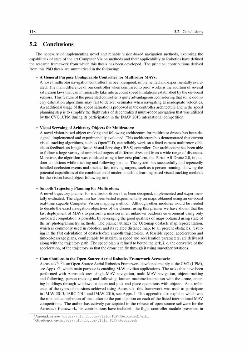
118 5.2. Conclusions
5.2 ConclusionsThe necessity of implementing novel and reliable vision-based navigation methods, exploring the
capabilities of state of the art Computer Vision methods and their applicability to Robotics have definedthe research framework from which this thesis has been developed. The principal contributions derivedfrom this PhD thesis are summarized in the following:
• A General Purpose Configurable Controller for Multirotor MAVs:A novel multirotor navigation controller has been designed, implemented and experimentally evalu-ated. The main difference of our controller when compared to prior works is the addition of severalsaturation laws that can intrinsically take into account speed limitations established by the on-boardsensors. This feature of the presented controller is quite advantageous, considering that some odom-etry estimation algorithms may fail to deliver estimates when navigating at inadequate velocities.An additional usage of the speed saturations proposed in the controller architecture and in the speedplanning step is to simplify the flight rules of decentralized multi-robot navigation that was utilizedby the CVG_UPM during its participation in the IMAV 2013 international competition.
• Visual Servoing of Arbitrary Objects for Multirotors:A novel vision-based object tracking and following architecture for multirotor drones has been de-signed, implemented and experimentally evaluated. This architecture has demonstrated that currentvisual tracking algorithms, such as OpenTLD, can reliably work on a fixed camera multirotor vehi-cle to feedback an Image Based Visual Servoing (IBVS) controller. Our architecture has been ableto follow a large variety of unmarked targets of different sizes and from a wide range of distances.Moreover, the algorithm was validated using a low-cost platform, the Parrot AR Drone 2.0, in out-door conditions while tracking and following people. The system has successfully and repeatedlyhandled occlusion events and tracked fast moving targets, such as a person running, showing thepotential capabilities of the combination of modern machine learning based visual tracking methodsfor the vision-based object following task.
• Smooth Trajectory Planning for Multirotors:A novel trajectory planner for multirotor drones has been designed, implemented and experimen-tally evaluated. The algorithm has been tested experimentally on maps obtained using an on-boardreal-time capable Computer Vision mapping method. Although other modules would be neededto decide the exact navigation objectives of the drones, using this planner we have shown that thefast deployment of MAVs to perform a mission in an unknown outdoors environment using onlyon-board computation is possible, by leveraging the good qualities of maps obtained using state ofthe art photogrammetry methods. The planner utilizes the Octomap obstacle map representation,which is commonly used in robotics, and its related distance map, to all present obstacles, result-ing in the fast calculation of obstacle-free smooth trajectories. A feasible speed, acceleration andtime-of-passage plans, configurable by maximum speed and acceleration parameters, are deliveredalong with the trajectory path. The speed plan is refined to bound the jerk, i. e. the derivative of theacceleration, of the trajectory so that the drone can fly through it using smoother rotations.
• Contributions to the Open-Source Aerial Robotics Framework Aerostack:Aerostack9,10is an Open-Source Aerial Robotics Framework developed mainly at the CVG (UPM),see Appx. G, which main purpose is enabling MAV civilian applications. The tasks that have beenperformed with Aerostack are: single-MAV navigation, multi-MAV navigation, object trackingand following, person tracking and following, human-machine interaction with the drone, enter-ing buildings through windows or doors and pick and place operations with objects. As a refer-ence of the types of missions achieved using Aerostack, this framework was used to participatein IMAV 2013, IARC 2014 and IMAV 2016, see Appx. I. This appendix also explains which wasthe role and contribution of the author to the participation on each of the listed international MAVcompetitions. The author has actively participated in the release of open-source software for theAerostack framework, his contributions have included: the flight controller module presented in
9Aerostack website: https://github.com/Vision4UAV/Aerostack/wiki10Github repository:https://github.com/Vision4UAV/Aerostack

Chapter 5. Conclusions and Future Work 119
Ch. 2, the aerial robotics visual servoing module presented in Chap. 3, the state estimator modulepresented in Appx. E and the simple kinematics simulator module based on the model presented inAppx. D.
• Participation in international MAV competitions and other public events:In order to ease the diffusion of results, the author has actively participated in public flight demon-strations, such as international MAV competitions, see Appx. I and other events, see Appx. J.Appx. I also explains which was the role and contribution of the author to the participation oneach of the listed international MAV competitions. The participation in such events has showcasedthe performance and increasing capabilities of Aerostack and it has promoted the further testing ofthe developed modules in different settings and applications, e. g. indoors and outdoors flight, nar-row corridors, passage through windows, landing in different conditions and so on. Teams of whichthe author has been part or in which colleagues have used modules explained in this dissertationand developed by author have participated in the following international aerial robotics competi-tions: 2016 DJI Developer Challenge - DJIC 2016, International Micro Air Vehicle Conference andFlight Competition 2016 - IMAV 2016, European Robotics Challenges 2014 - Simulation Chal-lenge 3 - EuRoC 2014, International Aerial Robotics Competition 2014 - Mission 7 - IARC 2014,International Micro Air Vehicle Conference and Flight Competition 2013 - IMAV 2013, Interna-tional Micro Air Vehicle Conference and Flight Competition 2012 - IMAV 2012 and the Concursoen Ingeniería de Control 2012 - CEA 2012.
5.3 Future WorkThe strong experimental basis of this work and the main research problems tackled during its realiza-
tion point towards the following areas for potential future work:
• In the area of control, estate estimation and dynamics modeling of drones, there are promising worksthat show that better models allow a much more precise estimation of the wind speed, or, in theabsence of wind, of the speed of the drone itself, see Sec. 3.2 and Appx. E.2. In addition to providingmore precise state estimates, the research in this direction may lead to safer flight maneuvering inenvironments that become very challenging under the presence of wind disturbances such as urbancorridors and indoor hallways. Another interesting area of research is the development of stateestimators that detect flight issues. Consider, for instance, soft collisions of the drone protectivehull with walls. Detecting such events may result in interesting behaviors such as control techniquesthat avoid the worsening of the flight situation, after the event is detected by the state estimator, likeavoiding a full crash against the said wall. Other physical contact events that are important to bedetected are the approach to the ground, the ceiling or walls, based on how these events affectthe flight of the drone; and determining the landing event more precisely, that may enable fasterlanding maneuvers on moving landing platforms. In the area of state estimation, many autopilotshave a very big dependence on the magnetometer sensor for the drone heading estimation. Therecurrently exist UAVs that can operate under magnetic interference by using multiple GPS sensors.In GPS-denied environments, for indoor navigation and flying near ferromagnetic infrastructure, itis required to use other sensor data for heading estimation, so as to decrease the dependence on themagnetometer sensor.
• In the area of visual servoing there is an strong inter-dependence between the performance of thevisual tracker and the successful realization of an object following task by a controller. Therefore,new methods could combine specific characteristics of the tracked objects and the surroundingenvironment into a better control strategy. For instance, it may be beneficial to select positionsrelative to the followed object that result in viewing angles without light glare reflections or strongshadows. In the same direction, the development of visual trackers that allow for object modelintrospection should be preferred. For instance, consider models that include the 3D structure of theobject or the reflective properties of the different surfaces of the object. A very interesting ongoingchallenge that may require model introspection is the International Aerial Robotics Competition(IARC) Mission 7, see Sec. I.4, where the drone needs to physically interact with ground robotsthat exhibit pseudo-random navigation behavior. From a navigation stand point, obstacle avoidance

120 5.3. Future Work
needs to be incorporated more strongly into the visual servoing task to enable following an objectthrough a cluttered environment, like a sportsman through a forest. In this sense, obstacles that aredifficult to map, such as trees, could be avoided considering their visual appearance rather than theirdifficult to reconstruct 3D structure.
• In the area of trajectory planning, the navigation control performs better when following smoothtrajectories, allowing faster motion. Additionally, less computer intensive trajectory generationalgorithms allow the drone to make rapid decisions while navigating in cluttered environments orwhile performing time critical operations. Since robots can move and affect which data is going tobe gathered for the mapping of the environment, another innovative research trend is acknowledgingthe inter-dependence in robotics of exploration, obstacle mapping and trajectory planning. Forinstance, the development of trajectory planning strategies that utilize obstacle maps that encodeuncertainty. There is also a trend to combine image processing and motion planning where thesetwo tasks are not separated in modules but rather solved together by means of deep learning. Someworks have already shown promising results in object grasping and door opening by robot armmanipulators, but similar techniques are still to be applied to drones.
• In the area of vision-based navigation, it would be important to increase the effort on the develop-ment of algorithms that can use a minimal setting of sensors and low power on-board computers.The research on novel vision-based and low computationally intensive pose estimation techniquesis of great importance for the development of autonomous very lightweight UAVs. These platformscan be rather harmless and may enable the use of drones around people in civilian applications.

Appendices
121


Appendix AScientific Dissemination
A.1 Journals
J. Pestana, J. L. Sanchez-Lopez, P. de la Puente, A. Carrio, P. Campoy. “A Vision-based QuadrotorMulti-robot Solution for the Indoor Autonomy Challenge of the 2013 International Micro Air VehicleCompetition”. In Journal of Intelligent and Robotic Systems. 2015. Springer Netherlands. Print ISSN:0921-0296. Online ISSN: 1573-0409.
J. L. Sanchez-Lopez, J. Pestana, P. de la Puente, P. Campoy. “A reliable open-source system archi-tecture for the fast designing and prototyping of autonomous multi-uav systems: Simulation and exper-imentation”. In Journal of Intelligent and Robotic Systems. 2015. Springer Netherlands. Print ISSN:0921-0296. Online ISSN: 1573-0409.
J. Pestana, I. Mellado-Bataller, C. Fu, J. L. Sanchez-Lopez, I. F. Mondragon, P. Campoy. “A Gen-eral Purpose Configurable Controller for Indoors and Outdoors GPS-Denied Navigation for MultirotorUnmanned Aerial Vehicles”. In Journal of Intelligent and Robotic Systems. 2013. Springer Netherlands.Print ISSN: 0921-0296. Online ISSN: 1573-0409.
J. L. Sanchez-Lopez, J. Pestana, S. Saripalli, P. Campoy. “An Approach Towards Visual Autonomousship board landing of a VTOL UAV”. In Journal of Intelligent and Robotic Systems. 2013. SpringerNetherlands. Print ISSN: 0921-0296. Online ISSN: 1573-0409.
L. Hernández Hernández, J. Pestana, D. Casares Palomeque, P. Campoy, J. L. Sanchez-Lopez “Iden-tificación y control en cascada mediante inversión de las no linealidades del cuatrirrotor del concurso decontrol inteligente CEA IFAC 2012”, in Revista Iberoamericana de automática e informática industrial,July–September 2013. Volume 10, Issue 3, pp. 356-367. ISSN: 1697-7912. ISSN: 1697-7920.
123

124 A.2. Publications in peer-reviewed conferences
A.2 Publications in peer-reviewed conferencesJ. Pestana, M. Maurer, D. Muschick, D. Adlakha, H. Bischof, F. Fraundorfer, “Package Delivery Ex-
periments with a Camera Drone”. In Austrian Robotics Workshop 2017, OAGM/AAPR2017 joint Work-shop.
J. L. Sanchez-Lopez, J. Pestana, P. Campoy. “A Robust Real Time Path Planner for the CollisionFree Navigation of Multirotor Aerial Robots in Dynamic Environments”. 2017 International Conferenceon Unmanned Aircraft Systems (ICUAS).
W. A. Isop, J. Pestana, G. Ermacora, F. Fraundorfer, D. Schmalstieg “Micro Aerial Projector - Sta-bilizing Projected Images Of An Airborne Robotics Projection Platform”. In IEEE/RSJ InternationalConference on Intelligent Robots and Systems, IROS2016
J. L. Sanchez-Lopez, R. A. Suárez Fernández, H. Bavle, C. Sampedro, M. Molina, J. Pestana, P.Campoy “AEROSTACK: An Architecture and Open-Source Software Framework for Aerial Robotics”. In2016 International Conference on Unmanned Aircraft Systems, ICUAS16
J. Pestana, R Prettenthaler, T Holzmann, D Muschick, C Mostegel, F Fraundorfer, H Bischof “GrazGriffins’ Solution to the European Robotics Challenges 2014”. In Austrian Robotics Workshop 2015,ARW2015
T Holzmann, R Prettenthaler, J. Pestana, D Muschick, G Graber, C Mostegel, F Fraundorfer, HBischof “Performance Evaluation of Vision-Based Algorithms for MAVs”. In Austrian Association forPattern Recognition Conference 2015, OAGM2015
J. L. Sanchez-Lopez, J. Pestana, JF Collumeau, Ramon Suarez-Fernandez, P. Campoy, M. Molina “Avision based aerial robot solution for the Mission 7 of the International Aerial Robotics Competition”. In2015 International Conference on Unmanned Aircraft Systems, ICUAS15
J. Pestana, J. L. Sanchez-Lopez, R. Suarez-Fernandez, J. F. Collumeau, P. Campoy, J. Martin-Cristobal, M. Molina, J. De Lope, and D. Maravall. “A Vision Based Aerial Robot solution for the IARC2014 by the Technical University of Madrid". In AUVSI International Aerial Robotics Competition 2014
J. Pestana, J. L. Sanchez-Lopez, P. de la Puente, A. Carrio, P. Campoy. “A Vision-based QuadrotorSwarm for the participation in the 2013 International Micro Air Vehicle Competition”. In 2014 Interna-tional Conference on Unmanned Aircraft Systems, ICUAS14
J. L. Sanchez-Lopez, J. Pestana, P. de la Puente, R. Suarez-Fernandez, P. Campoy. “A System forthe Design and Development of Vision-based Multi-robot Quadrotor Swarms”. In 2014 InternationalConference on Unmanned Aircraft Systems, ICUAS14
A. Carrio, C. Fu, J. Pestana, P. Campoy. “A Ground-Truth Video Dataset for the Development andEvaluation of Vision-based Sense-and-Avoid systems”. In 2014 International Conference on UnmannedAircraft Systems, ICUAS14
J. Pestana, J. L. Sanchez-Lopez, S. Saripalli, P. Campoy. “Computer Vision Based General ObjectFollowing for GPS-denied Multirotor Unmanned Vehicles”. In 2014 American Control Conference (ACC2014). Portland, Oregon (United States). June 4th - 6th 2014
J. Pestana, J. L. Sanchez-Lopez, S. Saripalli, P. Campoy. “Vision based GPS-denied Object trackingand Following for Unmanned Aerial Vehicles”. Best Paper Award Finalist in 2013 The 11th IEEEInternational Symposium on Safety, Security, and Rescue Robotics (SSRR 2013). Linköping (Sweden).Oct 21-26, 2013.

Appendix A. Scientific Dissemination 125
J. Pestana, I. Mellado-Bataller, C. Fu, J. L. Sanchez-Lopez, I. F. Mondragon, P. Campoy. “Ageneral purpose configurable navigation controller for micro aerial multirotor vehicles", In 2013 In-ternational Conference on Unmanned Aircraft Systems (ICUAS), pp. 557-564, 28-31 May 2013 doi:10.1109/ICUAS.2013.6564733
J. L. Sanchez-Lopez, S. Saripalli, P. Campoy, J. Pestana, C. Fu. “Visual Autonomous Ship BoardLanding of a VTOL UAV”. In 2013 International Conference on Unmanned Aircraft Systems (ICUAS’13).Atlanta, Georgia (USA). May 28-31, 2013.
J. Pestana, I. Mellado-Bataller, J. L. Sanchez-Lopez, C. Fu, I. F. Mondragon, P. Campoy. “FloorOptical Flow Based Navigation Controller for Multirotor Aerial Vehicles”. Robot 2013: First IberianRobotics Conference (ROBOT 2013).
J. L. Sanchez-Lopez, J. Pestana, P. de la Puente, A. Carrio, P. Campoy. “Visual Quadrotor Swarmfor IMAV 2013 Indoor Competition”. Robot 2013: First Iberian Robotics Conference (ROBOT 2013).
Jesús Pestana, Ignacio Mellado-Bataller, Fu Changhong, Jose Luis Sanchez-Lopez, Iván F. Mon-dragón, and Pascual Campoy “A Visual Guided Quadrotor for IMAV 2012 Indoor Autonomy Competitionand Visual Control of a Quadrotor for the IMAV 2012 Indoor Dynamics Competition”, at InternationalMicro Air Vehicle Conference and Flight Competition, IMAV 2012, July 2012
Changhong Fu, Jesús Pestana, Ignacio Mellado-Bataller, Jose Luis Sanchez-Lopez, and PascualCampoy “Visual Identification and Tracking for Vertical and Horizontal Targets in Unknown Indoor En-vironment”, at International Micro Air Vehicle Conference and Flight Competition, IMAV 2012, July2012
J. Pestana, J. L. Sánchez-López, I. Mellado, F. Changhong, P. Campoy, “AR Drone Identification andNavigation Control at CVG-UPM”, in XXXIII Jornadas de Automática, September 2012
J. Pestana, R. Bombín, E. Garcia, “Characterization of Magnetic Shape Memory Alloys (MSMA)Oriented to Periodic Actuation”, in 12th International Conference on New Actuators/6th InternationalExhibition on Smart Actuators and Drive Systems, Bremen, Germany, 2010
J. Pestana, R.Bombín, J. C. Arevalo and E. Garcia, “Characterization of emerging actuators for em-powering legged robots”, in 13th International Conference on Climbing and Walking Robots, CLAWAR,Nagoya, Japan, 2010
J. C. Arevalo, J. Pestana, F. Sanchez, J. F. Sarria and E. Garcia, “Impedance control of an agile-locomotion robotic leg”, in 13th International Conference on Climbing and Walking Robots, CLAWAR,Nagoya, Japan, 2010
A.3 Book ChaptersI. Mellado-Bataller, J. Pestana, M. A. Olivares-Mendez , P. Campoy, and L. Mejias, book chapter,
“MAVwork: a Framework for Unified Interfacing between Micro Aerial Vehicles and Visual Controllers”,in book “Frontiers of Intelligent Autonomous Systems”, serie “Studies in Computational IntelligenceSeries”, Springer, 2013, Volume 466, ISBN 978-3-642-35484-7, pp 165-179
A.4 Participation in Conference WorkshopsOct. 14, 2016: IEEE/RSJ International Conference IROS2016 Daejeon, Korea
Workshop on Vision-Based High Speed Autonomous Navigation of UAVs, presented “Vision based safenavigation for search and rescue drones” based on participation on the 2016 DJI Developer Challenge.


Appendix BUAVs and Multicopters
An Unmanned Aircraft (UA) or Unmanned Aerial Vehicle (UAV) is an aircraft without a human pi-lot on-board. These aircrafts are either piloted remotely by a human operator or autonomous, in whichcase the UAV does not depend on a human operator to fly safely. The degree of autonomy varies fromnavigation-only capabilities, to performing the decision-making necessary to perform a task or missionautomatically. Certainly, as it is common with current robotic technology, these systems cannot yet ac-complish general complex tasks by themselves; and full autonomy is still limited to specific use cases,such as automated data gathering for surveying purposes. However, autonomy does divide UAVs in thetwo major types specified above: Remotely Piloted Aircrafts (RPA), which require a human pilot, andAutonomous UAVs, which navigate themselves. It is remarked that RPA do have an on-board controlsystem that performs lower-level operations, such as tracking the attitude of the vehicle and adjusting itto follow the pilot’s commands. The main difference between both types is, thus, in the capability tonavigate themselves without direct human interaction.
A second term has been adopted to refer, not only to the aircraft, but to all the associated equipment.This term is Unmanned Aerial System (UAS), and includes the Ground Control Station (GCS), the com-munications, data links, telemetry and all the other equipment necessary to operate the UAV. The termUAS was initially used only for large sized systems, but it is currently more and more commonly usedfor small ones too. Both terms are correct, but one or the other should be utilized depending on whetheronly the aircraft or the whole system is alluded. In the same manner the term Remotely Piloted Aircraft(RPA) refers to the flying platform and the term Remotely Piloted Aircraft System (RPAS) refers also tothe rest of the equipment and instruments. Note that all RPAS are UAS, but not all UAS, for instance fullyautonomous ones, are RPAS.
UAVs can be classified by various characteristics, mainly weight, endurance and propulsion principle.The most common types, based on the latter, are fixed and rotary UAVs. Fixed wing aircraft produce liftforce by means of their forward speed and the shape of their wings, an example of them are airplanes.Various fixed-wing UAVs are shown in Fig. B.2. In rotary wing aircraft, or rotorcraft, the wings revolvearound a mast, and a common example are helicopters. There are other types of propulsion used in UAVs,for instance flapping wing aircraft move their wings as a bird to produce lift force. This thesis is focused
127
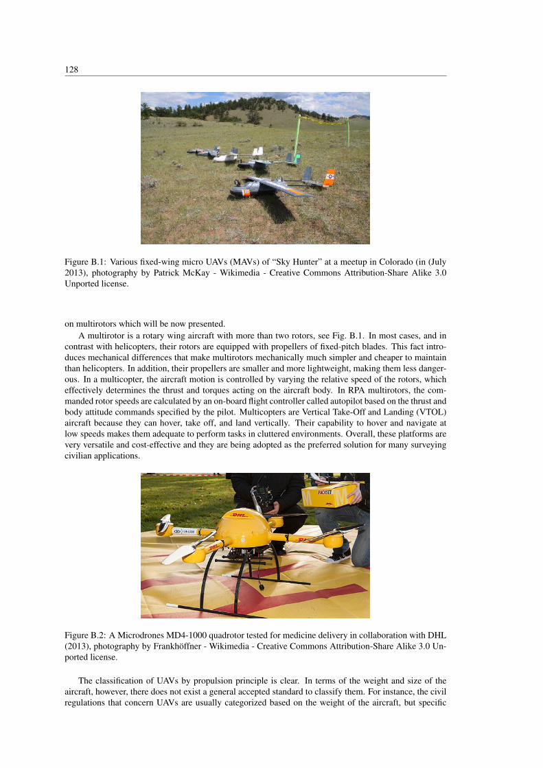
128
Figure B.1: Various fixed-wing micro UAVs (MAVs) of “Sky Hunter” at a meetup in Colorado (in (July2013), photography by Patrick McKay - Wikimedia - Creative Commons Attribution-Share Alike 3.0Unported license.
on multirotors which will be now presented.A multirotor is a rotary wing aircraft with more than two rotors, see Fig. B.1. In most cases, and in
contrast with helicopters, their rotors are equipped with propellers of fixed-pitch blades. This fact intro-duces mechanical differences that make multirotors mechanically much simpler and cheaper to maintainthan helicopters. In addition, their propellers are smaller and more lightweight, making them less danger-ous. In a multicopter, the aircraft motion is controlled by varying the relative speed of the rotors, whicheffectively determines the thrust and torques acting on the aircraft body. In RPA multirotors, the com-manded rotor speeds are calculated by an on-board flight controller called autopilot based on the thrust andbody attitude commands specified by the pilot. Multicopters are Vertical Take-Off and Landing (VTOL)aircraft because they can hover, take off, and land vertically. Their capability to hover and navigate atlow speeds makes them adequate to perform tasks in cluttered environments. Overall, these platforms arevery versatile and cost-effective and they are being adopted as the preferred solution for many surveyingcivilian applications.
Figure B.2: A Microdrones MD4-1000 quadrotor tested for medicine delivery in collaboration with DHL(2013), photography by Frankhöffner - Wikimedia - Creative Commons Attribution-Share Alike 3.0 Un-ported license.
The classification of UAVs by propulsion principle is clear. In terms of the weight and size of theaircraft, however, there does not exist a general accepted standard to classify them. For instance, the civilregulations that concern UAVs are usually categorized based on the weight of the aircraft, but specific

Appendix B. UAVs and Multicopters 129
category thresholds differ between countries. There does not exist a common regulation framework for allcountries, and each National Aviation Authority (NAA) has a similar but different set of rules concerningUAVs. A reliable perspective of how the European regulations will evolve to allow autonomous UAVs tofly in the common airspace is provided by the report (ERSG, 2013): “Roadmap for the integration of civilRemotely - Piloted Aircraft Systems into the European Aviation System”, written by the European RPASSteering Group (June 2013).
A comprehensive classification of UAVs, which is still applicable nowadays, was proposed by Blyen-burgh (Blyenburgh, 2006) and is backed by the Association for Unmanned Vehicles Systems International(UVS International). Two scholar articles that can also be consulted to understand this classificationare (Bento, 2008), which focuses on military UAVs, and (Watts et al., 2012) that describes also UAS usedfor civilian applications.

130 B.1. Appendix Bibliography
B.1 Appendix BibliographyBento, M. (2008). “Unmanned aerial vehicles: an overview”. Inside GNSS 3.1, pp. 54–61 (cit. on p. 129).Blyenburgh, P. v. (2006). “UAV Systems : Global Review”. In: Avionics’06 Conference. Amsterdam, The
Netherlands (cit. on p. 129).ERSG (2013). Roadmap for the integration of civil Remotely - Piloted Aircraft Systems into the European
Aviation System. Tech. rep. European RPAS Steering Group (cit. on p. 129).Watts, A. C., Ambrosia, V. G., and Hinkley, E. A. (2012). “Unmanned aircraft systems in remote sensing
and scientific research: Classification and considerations of use”. Remote Sensing 4.6, pp. 1671–1692(cit. on p. 129).
Appendix CMultirotor Software Interface
C.1 Introduction
In order to convert a commercial multirotor into an autonomous aerial robot several modules need tobe developed and integrated together. The development of software modules is eased by the utilization offrameworks that manage the data communication between them. To aid the development of the variousprocessing modules, the multirotor is adapted to provide a minimal set of functionalities and to commu-nicate using common interface commands and sensing data. This chapter describes the communicationframework, the abstract interface for the multirotor and an example of a software architecture used duringthe course of this thesis. The purpose of the main processing modules related to the works realized in thisthesis are introduced along with an example software architecture.
First the Robotics Middleware frameworks utilized for communicating data between processes areshortly introduced in Sec. C.2. Then, the abstract interface of the multirotor is described in Sec. C.3.Finally the software modules and architecture utilized to participate in the IMAV2012 competition areshortly discussed on Sec. C.4.
C.2 Robotics Middleware
There are many ways of putting the software of a robot together. Nowadays, there are various frame-works that allow each module to be developed separately; and that offer an easy way to communicateeach module with each other. The main goal of this approach is to free the developer of the burden ofputting together a complex communication system. Every member of the team can focus on their partof the project, without having to work on the underlying system architecture that takes care of commu-nicating the data. In robotics, this type of software is commonly known as middleware. Using popularrobotics middleware is very advantageous for open-source projects because it increases the shareabilityof the code. Any developer that is familiar with the utilized middleware knows how the communicationinterface works.
For instance, the Robot Operating System (ROS) (Quigley et al., 2009; Willow Garage, 2007) offers
131
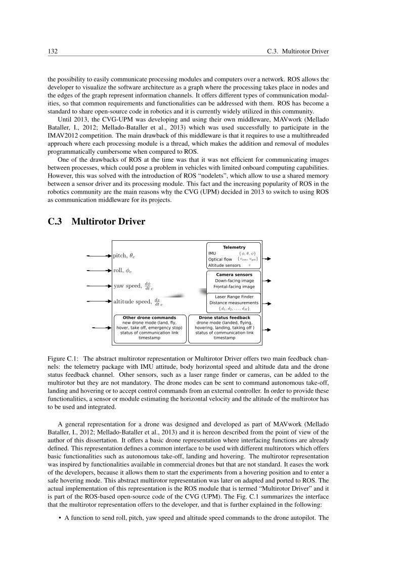
132 C.3. Multirotor Driver
the possibility to easily communicate processing modules and computers over a network. ROS allows thedeveloper to visualize the software architecture as a graph where the processing takes place in nodes andthe edges of the graph represent information channels. It offers different types of communication modal-ities, so that common requirements and functionalities can be addressed with them. ROS has become astandard to share open-source code in robotics and it is currently widely utilized in this community.
Until 2013, the CVG-UPM was developing and using their own middleware, MAVwork (MelladoBataller, I., 2012; Mellado-Bataller et al., 2013) which was used successfully to participate in theIMAV2012 competition. The main drawback of this middleware is that it requires to use a multithreadedapproach where each processing module is a thread, which makes the addition and removal of modulesprogrammatically cumbersome when compared to ROS.
One of the drawbacks of ROS at the time was that it was not efficient for communicating imagesbetween processes, which could pose a problem in vehicles with limited onboard computing capabilities.However, this was solved with the introduction of ROS “nodelets”, which allow to use a shared memorybetween a sensor driver and its processing module. This fact and the increasing popularity of ROS in therobotics community are the main reasons why the CVG (UPM) decided in 2013 to switch to using ROSas communication middleware for its projects.
C.3 Multirotor Driver
Telemetry
Optical flow
Altitude sensors
IMU
Laser Range Finder
Distance measurements
Camera sensors
Down-facing image
Frontal-facing image
Drone status feedbackdrone mode (landed, flying,
hovering, landing, taking off )status of communication link
timestamp
Other drone commandsnew drone mode (land, fly,
hover, take off, emergency stop)status of communication link
timestamp
Figure C.1: The abstract multirotor representation or Multirotor Driver offers two main feedback chan-nels: the telemetry package with IMU attitude, body horizontal speed and altitude data and the dronestatus feedback channel. Other sensors, such as a laser range finder or cameras, can be added to themultirotor but they are not mandatory. The drone modes can be sent to command autonomous take-off,landing and hovering or to accept control commands from an external controller. In order to provide thesefunctionalities, a sensor or module estimating the horizontal velocity and the altitude of the multirotor hasto be used and integrated.
A general representation for a drone was designed and developed as part of MAVwork (MelladoBataller, I., 2012; Mellado-Bataller et al., 2013) and it is hereon described from the point of view of theauthor of this dissertation. It offers a basic drone representation where interfacing functions are alreadydefined. This representation defines a common interface to be used with different multirotors which offersbasic functionalities such as autonomous take-off, landing and hovering. The multirotor representationwas inspired by functionalities available in commercial drones but that are not standard. It eases the workof the developers, because it allows them to start the experiments from a hovering position and to enter asafe hovering mode. This abstract multirotor representation was later on adapted and ported to ROS. Theactual implementation of this representation is the ROS module that is termed “Multirotor Driver” and itis part of the ROS-based open-source code of the CVG (UPM). The Fig. C.1 summarizes the interfacethat the multirotor representation offers to the developer, and that is further explained in the following:
• A function to send roll, pitch, yaw speed and altitude speed commands to the drone autopilot. The

Appendix C. Multirotor Software Interface 133
commands can be sent in an asynchronous fashion, at the pace defined by the user,
• Several drone modes can be commanded, offering autonomous take off and landing. During flightthe drone can be commanded to enter position hold mode (hover mode), where the drone approx-imately stays in position by using the speed estimates. The ‘flying’ mode obeys the attitude andaltitude speed commands sent by the user application,
• Timestamps and the status of the communication link are exchanged between the drone and theapplication with no intervention from the client application,
• The telemetry feedback channel sends back IMU attitude, body horizontal speed an altitude data,
• The actual drone mode is sent back to the client application inside the telemetry package.
• Other sensors, such as a laser range finder or cameras, can be added to the multirotor but they arenot mandatory,
• From the user point of view, the feedback channels are independent threads that are woken up whena new measurement is available. And the commands are transfered to the multirotor autopilot assoon as they are received.
In order to provide the take-off, landing and hovering functionalities, a sensor or module estimatingthe horizontal velocity and the altitude of the multirotor has to be integrated with the Multirotor Driver.This data is readily available in the AR Drone, where it is obtained using an ultrasound altimeter and aground optical flow speed sensor. Other drones have to be adapted by using appropriate sensors dependingon the application.
C.3.1 Notes on the adaptation of the Asctec Pelican to the Multirotor DriverThe Pelican does not natively provide support for the described MAVwork framework. In order to add
it, by the members of the CVG (UPM) as part of prior works and for the participation in IMAV2012, aserial communication link was first implemented between the high-level autopilot board and the onboardIntel Atom running Linux, which is used as main processing platform. In this way, a framework-compliantproxy could be implemented on the Atom onboard computer, using the WiFi interface for networking. Forthe IMAV2012, the Pelican proxy was interfaced with a Hokuyo range finder, whose readings were sentto the control application through a camera channel.
The Pelican autopilot does not naturally support the MAV1 protocol, used by MAVwork (MelladoBataller, I., 2012; Mellado-Bataller et al., 2013). It neither interprets commands in the required format norgives navigation information as expected by the protocol. Therefore, some software adaptations involvingreference frame changes and conversion of units were carried out on the already available commands andfeedback to suit the MAV1 specification. However, some measures, like the drone speed estimate or thealtitude, required also the addition of new hardware and special processing. For the altitude measurements,a couple of ultrasound sensors were added. When they point to the ground they can give a much betterestimate than the Pelican internal altitude sensor, which is based on air pressure measurements. Thedrone speed is estimated with a camera, also pointing to the ground. At every frame, the optical flow iscomputed with the OpenCV implementation of the pyramidal Lucas-Kanade algorithm for some imagefeatures selected by the Shi-Tomasi method.
The ROS version of the Multirotor Driver for the Asctec Pelican was integrated with the PX4Flowsensor (Honegger et al., 2013), which provides altitude and horizontal speed measurements in a simi-lar manner to the AR Drone. This version of the driver was first used to participate in the IARC2014competition.
By using the Multirotor Driver, the Pelican and the AR Drone offer a common interface and theirbehaviors are similar. In 2012, a control application for them was implemented using MAVwork (MelladoBataller, I., 2012), which later came to be adapted to the common Multirotor Driver interface in ROS.MAVwork exposes an Application Programming Interface (API), independent of the drone type, throughwhich visual control applications can communicate with MAVs without worrying about their hardwarespecifics. Deeper explanations of how the framework is implemented can be found on (Mellado Bataller,I., 2012; Mellado-Bataller et al., 2013; Pestana et al., 2012). Thanks to this approach, the trajectorycontroller used in the IMAV2012 dynamics challenge was first tested and debugged on a Parrot AR Drone,

134 C.4. Example Software Architecture (IMAV2012)
which we often use as prototyping platform. Once tests showed that the software was bug-free and robust,the controller was run and fine-tuned on the Pelican without changing the application structure; only theparameters of the dynamic controllers were modified to suit the Pelican flight dynamics.
C.4 Example Software Architecture (IMAV2012)
Multirotorautopilot
IMU, magnetometer& pressure sensor
ESCs & motors
MultirotorDriver
AutopilotBoard
Cameraoptical flow
speedestimation
ultrasoundaltimeter
HokuyoLaser Range Finder
StateEstimator & particle
filter
TaskScheduler
TrajectoryController
UserInterface
& monitoring
fused IMU
horiz. speed
altitude
flight-mode command
commandstrajectorycommand
state estimate
laser scan
autopilotinterface
Onboard Computer& Sensors
Figure C.2: Overview of the software architecture utilized to participate in the IMAV2012 competition.The autopilot takes care of the data acquisition and low-level control tasks of the multirotor. The onboardcomputer acquires information from additional sensors, a camera, an ultrasound altimeter and a Hokuyolaser range finder, and uses it to enable the multirotor to perform the autonomous flight in the competition.The Multirotor Driver centralizes the communications with the autopilot and offers the practical flight-mode commands interface by taking care of middle-level tasks such as take-off, land and hover. The stateestimator assesses the current position and speed of the multirotor based on the sensor data. It also feedsits estimate to the particle filter that can calculate a drift-free position estimate by comparing the laserscans to the known obstacle map. The controller calculates attitude and altitude speeds commands forstabilizing the drone and follow trajectory commands. The competition dynamics challenge is achievedautonomously by using a rigid task scheduler that leverages the discussed software architecture. It moni-tors the state of the drone and its battery status and issues a series of flight-mode and trajectory commandsas the realization of the navigation tasks proceeds and are accomplished.
The development of an autonomous robot requires engineering many different software modules. Forthe participation in the IMAV2012, the software architecture was implemented using a single programin a multi-threaded approach based on MAVwork (Mellado Bataller, I., 2012; Mellado-Bataller et al.,2013; Pestana et al., 2012). The following list of modules and Fig. C.2 describe the software that wasrunning during the competition, which allowed to follow trajectories and perform the dynamics challengeautonomously in the environment described by the competition rules:
• Low-level sensing, control and hardware interfaces: many multirotors provide these functionali-ties out of the box, these tasks being accomplished by a board called autopilot. However, manycommercial drones do not provide a convenient way to command the drone from an onboard com-puter, and are only designed to be flown by human pilots. The information from several sensors isacquired to determine the attitude of the aerial robot and, usually using GPS, its position. Theseinformation together with the flight commands is used to stabilize the flight of the multirotor.
• Interfacing the onboard computer with the autopilot and various sensors: each sensor module isinterfaced using the libraries provided by the manufacturer. A multi-threaded approach or separateprograms that communicate through a robotics middleware are used to obtain the sensor data assoon as it is available. These interfaces have to be reliable and thus require debugging and testing.
Appendix C. Multirotor Software Interface 135
• A state estimation module provides a real-time assessment of the position, attitude and velocity ofthe flying robot, based on the information available in the sensor measurements.
• A controller module which principal objective is to allow other modules to move the vehicle with amore friendly set of commands. In the case of multirotors a position controller allows commandingthe multirotor directly in the {x, y, z, ψ} coordinates, which represent its position and heading.Another options which was used in the IMAV2012, is to make a controller that can follow trajectorycommands. The control module has to be able to safely communicate with the estimation modulein a bidirectional fashion. The estimation algorithm can benefit from knowing which commandsthe controller is sending to the multirotor autopilot, and the controller needs the estimation of theposition and velocities of the robot to calculate the commands.
• A task scheduler, which is in charge of chaining a set of steps that accomplish the mission ob-jectives. The task scheduler requires to communicate with the priorly explained modules: theMultirotor Driver, the Trajectory Controller and the State Estimator. The communications with theestimation module and additional sensors are used to update the status of accomplishment of themission objectives; and the scheduler uses the controller to command the robot where to move next.
• A user interface, either graphical or through a simple console interface: the user needs to be ableto monitor what the robot is doing and if necessary to take command over the robot, basicallydeactivating the task scheduler and/or controller; and sending commands himself.

136 C.5. Appendix Bibliography
C.5 Appendix BibliographyMellado Bataller, I. (2012). A new framework for interfacing with MAVs. https://github.com/
uavster/mavwork (cit. on pp. 132–134).Honegger, D., Meier, L., Tanskanen, P., and Pollefeys, M. (2013). “An open source and open hardware
embedded metric optical flow cmos camera for indoor and outdoor applications”. In: Robotics andAutomation (ICRA), 2013 IEEE International Conference on. IEEE, pp. 1736–1741 (cit. on p. 133).
Mellado-Bataller, I., Pestana, J., Olivares-Mendez, M. A., Campoy, P., and Mejias, L. (2013). “MAVwork:a framework for unified interfacing between micro aerial vehicles and visual controllers”. In: Frontiersof Intelligent Autonomous Systems. Springer, pp. 165–179 (cit. on pp. 132–134).
Pestana, J., Mellado-Bataller, I., Fu, C., Sanchez-Lopez, J. L., Mondragon, I. F., and Campoy, P. (2012).“A Visual Guided Quadrotor for IMAV 2012 Indoor Autonomy Competition and Visual Control ofa Quadrotor for the IMAV 2012 Indoor Dynamics Competition”. International Micro Air Vehicle(IMAV), 2012 Conference and Flight Competition (cit. on pp. 133, 134).
Quigley, M., Gerkey, B., Conley, K., Faust, J., Foote, T., Leibs, J., Berger, E., Wheeler, R., and Ng,A. (2009). “ROS : an open-source Robot Operating System”. In: IEEE International Conference onRobotics and Automation (ICRA 2009) (cit. on p. 131).
Willow Garage, S. A. I. L. (2007). Robot Operating System (ROS). http://www.ros.org/wiki/(cit. on p. 131).

Appendix DMultirotor dynamics modeling
D.1 IntroductionThe purpose of this appendix is to present the multirotor models that have been used during the
course of this PhD Thesis. Sec. D.2, describes the rigid body dynamics of the multirotor. This model isuseful to understand the attitude controller which in the multirotors utilized in this thesis has always beenexecuted inside the autopilot, which motivates the next section. For medium-level controllers the rigidbody model, Sec. D.3, is augmented to simulate a multirotor with an autopilot board that accepts the usualmultirotor attitude and thrust or altitude velocity command set. For the design of the Extended KalmanFilter (EKF) and the controllers designed and implemented as part of this PhD Thesis simplified modelswere considered, so that only the main characteristics of the multirotor dynamics system are represented.These simplified models are presented in the rest of this chapter. Sec. D.4 introduces a simplification to2 degrees of freedom of the multirotor model, where the simulated vehicle flies in a horizontal plane andwith a constant heading. A complete simplified model for the multirotor vehicle is proposed in Sec. D.5,which is inspired in the previously discussed models from Secs. D.3 & D.4. The last section, Sec. D.6,summarizes the uses of these models during the progress of this PhD Thesis.
D.2 Model based on rigid body dynamicsThe Fig. D.1 shows the free body diagram of a quadrotor. The principal magnitudes that affect the
dynamic movement of this aircraft are: the mass properties of the vehicle body, and the forces and torquesgenerated by the propellers. The following symbols describe them and are used in later equations anddiscussion:
• the position of the quadrotor is denoted by the {x, y, z} coordinates,
• the attitude of the vehicle is represented by the yaw, pitch and roll Euler angles. Which are denoted:{φ , roll}, {θ ,pitch} and {ψ,yaw},
137

138 D.2. Model based on rigid body dynamics
φψ
θ
T2
T4
T1T3 M2
M3M1
M4
Figure D.1: Free body diagram of a quadrotor. The four propellers, and each of their performed thrust Tiand torque Mi are labeled 1-4. The euler angles are denoted {φ , roll}, {θ ,pitch} and {ψ,yaw}
• the quadrotor rigid body is characterized by its mass m and its three principal mass moments ofinertia {Ix, Iy, Iz},
• each propeller i generates a thrust Ti and a heading torque Mi,
• the l constant is the distance between the centers of each pair of opposite propellers, such us pro-pellers 1 and 3 in Fig. D.1,
• each propeller rotates at speed ωi; and its thrust causes a torque with respect to the center of massof the quadrotor that can tip the aircraft body frontward, backward or sideways.
The quadrotor rigid body dynamics model, see Eq. D.1 and Fig. D.1, is inferred by considering theeffects of the forces described above and is explained in multiple articles (Hoffmann, Gabriel M et al.,2008; Michael et al., 2010).
Ix φ = ψ θ (Iy− Iz)+(l/√
2)(+T1−T2−T3 +T4)
Iy θ = φ ψ (Iz− Ix)+(l/√
2)(−T1−T2 +T3 +T4)Iz ψ = θ φ (Ix− Iz)+(−M1 +M2−M3 +M4)mx = (−sφ sψ− cφ sθ cψ) ∑
4i=1 Ti
my = (−cφ sθ sψ + sφ cψ) ∑4i=1 Ti
mz = mg− cθ cφ ∑4i=1 Ti
(D.1)
It is generally accepted to approximate Ti and Mi as Ti = kT ·ω2 and Mi = kM ·ω2, where ω , kMand kT are the propeller speed and two propeller characteristic constants. The differences between thesetheoric equations and the reality are dealt with by the attitude controller implemented in the autopilot.The attitude controllers can be PIDs, and still provide good results (Hoffmann, Gabriel M et al., 2008;Michael et al., 2010). However, this is suboptimal because the attitude of the quadrotor determines itslinear acceleration. Thus the derivatives of the acceleration are determined by the rotation velocity of thequadrotor body. Nonlinear controllers based on this observation outperform its PID counterparts (Fritschet al., 2012), but require the usage of more complex state estimators that estimate the correspondinglyaugmented state of the aircraft, which needs to estimate the derivatives of the acceleration.
Using the above mentioned relationships Ti = kT ·ω2 and Mi = kM ·ω2, the input to this model isthe speed of each propeller, and the output would be the position and attitude of the quadrotor. Theseinputs correspond to the autopilot outputs, because the vehicle has interface boards, called ElectronicSpeed Controllers (ESC), that receive the autopilot commands and approximately control the speed of thepropeller rotors.
D.2.1 Brief explanation of the Low-level and Mid-level control of a quadrotorThe terms of the Eq. D.1 are explained here, and then their relations to the low-level and mid-level
control laws are clarified. This point of view of the problem helps to better understand the quadrotor rigidbody model, and how a cascade of PID controllers can be used to command the aircraft. The terms inEq. D.1 can be understood as follows:
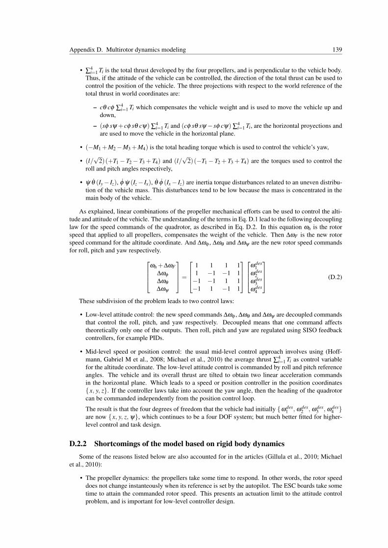
Appendix D. Multirotor dynamics modeling 139
• ∑4i=1 Ti is the total thrust developed by the four propellers, and is perpendicular to the vehicle body.
Thus, if the attitude of the vehicle can be controlled, the direction of the total thrust can be used tocontrol the position of the vehicle. The three projections with respect to the world reference of thetotal thrust in world coordinates are:
– cθ cφ ∑4i=1 Ti which compensates the vehicle weight and is used to move the vehicle up and
down,
– (sφ sψ +cφ sθ cψ) ∑4i=1 Ti and (cφ sθ sψ− sφ cψ) ∑
4i=1 Ti, are the horizontal proyections and
are used to move the vehicle in the horizontal plane.
• (−M1 +M2−M3 +M4) is the total heading torque which is used to control the vehicle’s yaw,
• (l/√
2)(+T1−T2−T3 +T4) and (l/√
2)(−T1−T2 +T3 +T4) are the torques used to control theroll and pitch angles respectively,
• ψ θ (Iy− Iz), φ ψ (Iz− Ix), θ φ (Ix− Iz) are inertia torque disturbances related to an uneven distribu-tion of the vehicle mass. This disturbances tend to be low because the mass is concentrated in themain body of the vehicle.
As explained, linear combinations of the propeller mechanical efforts can be used to control the alti-tude and attitude of the vehicle. The understanding of the terms in Eq. D.1 lead to the following decouplinglaw for the speed commands of the quadrotor, as described in Eq. D.2. In this equation ωh is the rotorspeed that applied to all propellers, compensates the weight of the vehicle. Then ∆ωF is the new rotorspeed command for the altitude coordinate. And ∆ωφ , ∆ωθ and ∆ωψ are the new rotor speed commandsfor roll, pitch and yaw respectively.
ωh +∆ωF∆ωφ
∆ωθ
∆ωψ
=
1 1 1 11 −1 −1 1−1 −1 1 1−1 1 −1 1
ωdes1
ωdes2
ωdes3
ωdes4
(D.2)
These subdivision of the problem leads to two control laws:
• Low-level attitude control: the new speed commands ∆ωφ , ∆ωθ and ∆ωψ are decoupled commandsthat control the roll, pitch, and yaw respectively. Decoupled means that one command affectstheoretically only one of the outputs. Then roll, pitch and yaw are regulated using SISO feedbackcontrollers, for example PIDs.
• Mid-level speed or position control: the usual mid-level control approach involves using (Hoff-mann, Gabriel M et al., 2008; Michael et al., 2010) the average thrust ∑
4i=1 Ti as control variable
for the altitude coordinate. The low-level attitude control is commanded by roll and pitch referenceangles. The vehicle and its overall thrust are tilted to obtain two linear acceleration commandsin the horizontal plane. Which leads to a speed or position controller in the position coordinates{x, y, z}. If the controller laws take into account the yaw angle, then the heading of the quadrotorcan be commanded independently from the position control loop.
The result is that the four degrees of freedom that the vehicle had initially {ωdes1 , ωdes
2 , ωdes3 , ωdes
4 }are now {x, y, z, ψ}, which continues to be a four DOF system; but much better fitted for higher-level control and task design.
D.2.2 Shortcomings of the model based on rigid body dynamicsSome of the reasons listed below are also accounted for in the articles (Gillula et al., 2010; Michael
et al., 2010):
• The propeller dynamics: the propellers take some time to respond. In other words, the rotor speeddoes not change instanteously when its reference is set by the autopilot. The ESC boards take sometime to attain the commanded rotor speed. This presents an actuation limit to the attitude controlproblem, and is important for low-level controller design.

140 D.3. Model based on rigid body dynamics with autopilot
• Aerodynamic disturbances: aside from wind disturbances, there are aerodynamic disturbances thatdo not manifest in normal navigation, and appear for example during a stall turn maneuver (Hoff-mann, G.M. et al., 2009).
• The communication delay between the ESCs and the controller which might be implemented onthe autopilot, an onboard computer or a groundstation,
• The damping coefficients in the horizontal plane, that model the aerodynamic friction, serve topartly explain the response time of the linear speed dynamics of the quadrotor and to have a goodsteady-state model fixing the correspondence between roll and pitch values to steady-state horizon-tal speed values. It is also important to model the maximum speed of the vehicle, because it is alimiting factor for the velocity controller design. For example, based on our experiments, whenusing the indoors hull the Parrot AR Drone 1 has a maximum speed of about 2.5 m/s, even tiltingthe vehicle further will not achieve faster speeds.
• Regarding the aerodynamic friction, recent studies (Abeywardena et al., 2013; Leishman et al.,2014) have identified the horizontal aerodynamic friction of the propellers as a mayor force con-tributing to the dynamics of the quadrotor that affects the readings of the accelerometers in suchvehicles. These frictions are explained as blade flapping, profile and induced drag forces on thepropellers.
Some reasons for not using the rigid body model are:
• A multirotor with a closed autopilot software, such as the AR Drone does not accept rotor speedcommands, but roll, pitch and yaw speed commands; for the altitude the are two possibilites eitheran altitude speed or a thrust command.
• Most closed autopilots that are intended for private or public developers give at least attitude mea-surements. But in order to use the acceleration measurements from the IMU the bias affecting themneeds to be identified in real-time, for example using a Kalman Filter formulation.
• For the linear speed or position controller design of a quadrotor with an embedded attitude con-troller, there are other parameters that need to be identified. All saturations that affect the modeland the response time of the variables that are to be controlled have to be . The following are listof such parameters that are considered in the identification process: the maximum speeds that thevehicle can reach, the response time of the attitude angles (as controlled by the autopilot), the re-sponse time of the horizontal speed after step commands in pitch and roll; the response time of thealtitude speed to a step command; and similarly for the yaw speed. A methodology to obtain thesedata will also be explained in later sections; it basically requires to make judicious experimentaltests.
To solve the first problem, in the next section, Sec. D.3, an attitude controller is added to the model.For the last issue some simplified models have been developed in Sec. D.4&D.5.
D.3 Model based on rigid body dynamics with autopilotThe difference between this model and the rigid body model is on the inputs and outputs. The inputs
are not rotor speed comands, but roll, pitch and yaw speed commands; and for the altitude there aretwo possibilities either an altitude speed or a thrust command. These corresponds to the usual inputsof a multirotor autopilot. Similarly, the outputs are selected to be the same as the autopilot availablemeasurements. This would result in a model with the block diagram shown in Fig. D.2:
The idea is to imitate the response of a multirotor that has already a low-level controller implementedin the autopilot board. A way of obtaining such a model is the following, see Fig. D.2:
• Identify the rigid body model, as explained in Sec. D.2.
• Perform experimental tests to identify the saturation limits of the system: φmax, θmax, ψmax, zmax andvxymax. vxymax is the maximum horizontal speed of the multirotor. It is also worthwhile to determinethe maximum speed that the speed measurement method can safely estimate.

Appendix D. Multirotor dynamics modeling 141
Rotor speed
Decoupling Law,
Propeller Dynamics
Rigid Body
Dynamics model
Attitude controller
Roll
Pitch
Yaw
Thrust
omega_roll
omega_pitch
omega_yaw
M_i
Thrust_i measurements
IMU feedback
Figure D.2: Rigid body model with autopilot. The altitude control is added if it is present on the autopilot.The most important thing to do, is to have a model that has the same inputs and outputs as the actualmultirotor. And that both have the same saturation limits and response times, among other characteristics,as the real system.
• Perform experimental tests to identify the critical response times of the multirotor:
– Response times on φ , θ , ψ , z.
– Estimate the response time of the horizontal speed. This can be done measuring the speedafter a roll or a pitch step command.
• Implement the “Rotor speed Decoupling Law, and Propeller Dynamics” box: the thrust commandmust be converted to ∆ωF using the relation T hrust = kT (ωh +∆ωF)
2. Then the decoupling lawspecified in Eq. D.2 must be implemented to pass from ∆ωi commands to ωi references for the ESCboards. Then the propellers can be modeled as a first order system with an appropiate responsetime. The output of these blocks would be the simulated rotor speeds ωi. For example in (Michaelet al., 2010) a first order system with response time of 50 ms was used for the propeller dynamics,it is probable that the response time is bigger for quadrotors of bigger size such as the AsctecPelican, Sec. H.1. And finally the rotor speeds are converted to thrusts and heading torques usingthe relations Ti = kT ·ω2 and Mi = kM ·ω2.
• The attitude controller and, if necessary, the altitude controller have to be implemented, for instancePID controllers can be used. The most important thing is that the simulated system must presentresponse times similar to the experimental data from the identification tests and to the multirotoritself.
pitch
roll
d(Yaw)/dt
X, Y, Z
Roll,Pitch,Yaw
d(Alt)/dt
Figure D.3: AR Drone black-box model. The specified inputs match the real system’s. The Euler anglesand the altitude outputs are available from the AR Drone telemetry data. To the contrary, the only availabledata from the drone about the X and Y directions are speed estimates. These estimates are obtained bymeans of a down-facing camera and optical flow algorithms.

142 D.4. Simplified model with altitude and yaw hold
A good example of a multirotor that can be represented by the rigid body model with autopilot isthe Parrot AR Drone. The input commands of the drone are roll, pitch, yaw speed and altitude speedcommands, as illustrated in Fig. D.3. The software of the autopilot is totally closed, and the measurementsare communicated to the host computer via WiFi every 60-70 ms. The available measurements from thedrone are attitude and altitude measurements, and about the X and Y coordinates only speed measurementsare available; the parrot does not have a GPS receiver. The horizontal speed measurements are obtainedfrom the down-facing camera image by means of visual odometry algorithms (Bristeau et al., 2011).
Telemetry
Optical flow
Altitude sensors
IMU
Laser Range Finder
Distance measurements
Various camerasDown-facing image
Frontal-facing image
Figure D.4: Pelican black-box model as equipped by the CVG_UPM team for the IMAV2012. Thespecified inputs match the real system’s. The Euler angles are available from the Pelican telemetry data.Two sonar altitude sensors were added using a USB mini acquisition board, “PhidgetInterfaceKit 2/2/2”,to obtain an altitude measurement. The available data from the quadrotor about the X and Y directions arespeed measurements obtained by means of an optical flow algorithm applied to down-facing images; andthe measurement from a Hokuyo Scanning Laser Range Finder that was added to perform localization.
Another good example of a multirotor that can be represented by the rigid body model with autopilotis the Asctec Pelican. The vehicle was used as illustrated in Fig. D.4 to participate on the IMAV2012international competition. The autopilot was configured to accept attitude and thrust commands. TheAsctec Pelican has a closed embedded autopilot that performs the attitude control, and that providesmeasurements regarding the low-level state of the vehicle. Two sonar sensors where added to obtainaltitude measurements. A down-facing camera is used to have an image of the ground, the optical flowprocessing on its images combined with the altitude measurements results on a speed estimate. Finally aHokuyo Scanning Laser Range Finder was added to perform localization.
D.4 Simplified model with altitude and yaw hold
This model was developed to participate in the international competition “Concurso de Ingenieríade Control 2012, Control Autónomo del seguimiento de trayectorias de un vehículo cuatrirrotor”, whichfinal phase was held in Vigo, Galicia; in September 2012. This competition will be called CEA 2012competition for the rest of this appendix. The model is easier to identify and control, because it has only2 inputs and 2 outputs. The altitude and yaw heading are not modeled. Only the roll and pitch commandsare available; and the outputs of the model are only related to the X and Y coordinates.
To simplify the identification and control problems, the organizers of the CEA 2012 competition haddecided to constrain the quadrotor movement to the horizontal plane and also to fix the yaw heading.Thus, leaving roll and pitch as the only command variables. An inspection of the underlying dynamicmodel, from Eq. D.1, reveals that the pitch angle controls the speed in the X direction, and the roll anglecontrols the speed in the Y direction.
Taking into account these contraints the simplified model depicted in Fig. D.5 is proposed:

Appendix D. Multirotor dynamics modeling 143
pitch
roll
commandsaturation
+aerodynamic
friction+
non-symmetric behavior
vx
pitchLTI
system
rollLTI
system
1/s
vy
1/s
x
y
non-linearfunction
linear time-invariant (LTI)transter function
vx_ss
vy_ss
Figure D.5: Quadrotor simplified model, only the pitch and roll inputs are kept, along with the mainresulting quadrotor behavior.
• A non-linear function models and fixes the steady-state correspondance between {φ ,θ} and{vx,vy}. The quadrotor characteristics modeled by this non-linear function are:
– aerodynamic friction: it can be expressed as a correspondance between constant input val-ues and steady-state speed values {vx_ss,vy_ss}. This relationship can be non-symmetric,[vx_ss, vy_ss] = f(θ , φ), i. e. presenting different maximum speed values for each direction.
– maximum tilt angle: expressed by a 2D command saturation (φ/φmax)2 + (θ/θmax)
2 ≤ 1
• The dynamics of the quadrotor are modeled by a linear time invariant (LTI) system, i. e. a transferfunction. The LTI systems model: the roll and pitch closed loop response, and the resultant dampedspeed response. Instead of including all the high frequency poles and the whole physical behaviorof the drone, the actual transfer function can be simplified and just include the slowest poles anddynamics.
D.5 Complete multirotor simplified model
The model presented in this subsection retains the simplicity of the previous model in the sense thatthe identification experimental tests are easy to perform. The quadrotor movement in the horizontal planeis strongly determined by the aerodynamic friction and the attitude offset of the IMU. It is really importantthat the friction stays opposite to the actual speed of the quadrotor in the world frame, being independentof the yaw orientation of the vehicle.
pitch
vx
LTIsystem
1/s
vy
1/s
x
y
aerodynamicfriction
model in vehicle
reference frame
pitchc
rollLTIsystem
rollc
dyawLTIsystem
dyawc1/s
yaw
dzLTIsystem
dzc1/s
z
thrust horizontal proyection calculation
ktr
ktr
changeto world
referenceframe
vx
vy
Fxm_friction
Fym_friction
Fxm
Fym
1/s1/s
1/s
-
-
axm
aym
ax
ay
yaw
Figure D.6: Complete multirotor simplified model, all inputs are taken into account. The altitude andyaw loops are supposed to have a speed controller, so that the model roughly identifies the closed loopbehavior.
Taking into account these constraints the simplified model depicted in Fig. D.6 is proposed:

144 D.5. Complete multirotor simplified model
• A non-linear function models the aerodynamic friction, which can be specified in the vehicle refer-ence frame. In order to obtain a friction force opposite to the speed in the world frame the modelincludes a change of the reference coordinates from the world to the vehicle frame:
– The roll and pitch angles {φ ,θ} produce a force specified in the vehicle frame: {Fx =−mgsin(θ),Fy = mgsin(φ)}. This force is a gross magnitude, from which the friction mustbe substracted.
– Aerodynamic friction: the friction is specified by a non-linear function that depends on the ori-entation of the horizontal speed, α , in the vehicle frame and on the modulus of the speed. Ex-perimental data is being fitted to the following model: Ff riction = c1(α) ( |vm| + c2(α) ) vm.The vehicle speed is changed from the world frame to the body frame, using the yaw angle.And then the aerodynamic friction equation is used. The result is the friction force in the bodyframe coordinates, that can now be subsctracted from the gross horizontal thrust force.
– The aerodynamic friction is substracted to the horizontal component of the quadrotor’s thrust,obtaining a resulting pseudo-acceleration. The acceleration that will be applied to calculatethe speed is proportional to the one calculated before.
– Horizontal speed response time: the pseudo-acceleration is multiplied by a positive gain, totune the response time to experimental data. Then an artificial gain ktr is added to the model,so that the response time of the model can be tuned. The relation between this constant andthe approximate obtained response time is: tr =
3ktrc1(2|vm|+c2)
. The obtained response is similarto a first-order model response.
• The other dynamics of the quadrotor are modeled by several linear time invariant (LTI) systems,i. e. transfer functions.
• The fastest multirotor dynamics that are modeled explicitly by the model are the pitch and rollangles. In the AR Drone the response time of these variables is about 150-300 ms; and the responsetime of the yaw speed command and altitude speed is about 500 ms. In the rigid body model,Secs. D.2 & D.3, the fastest response time is the propeller response, which will respond in about50 ms. This fact, makes that the system can be simulated at slower sampling times, and also thatthere are less state variables; which may be useful for certain purposes.
An advantage of the model is that several saturation limits of the system can be directly specified:
• maximum roll, pitch, altitude speed and yaw speed can be fixed putting saturation limits at the inputof the model.
• the aerodynamic friction together with the roll and pitch limits fix the maximum horizontal speedof the multirotor model.
• disturbances can be added to the model, for example, pitch and roll disturbances. This would makethe quadrotor not hover in position with zero pitch and roll commands.
Another convenience of this model is that the response times of the principal variables can be fixedeasily in the model:
• the roll, pitch, altitude speed and yaw speed response times are fixed by their respective (LTI)systems.
• the response time of the horizontal speed is fixed by ktr.
Some other interesting facts about the model are:
• The multirotor model can perform a horizontal circle with similar inputs as the real multirotor. Notests have been done checking actual values of both inputs. The meaning of this is that with a con-stant command of roll, pitch and yaw speed, a multirotor will perform horizontal circle trajectoriesof varying radius.
Appendix D. Multirotor dynamics modeling 145
• The aerodynamic friction is always parallel to the current speed of the multirotor. For instance, ifthe vehicle has a certain velocity direction and then the pitch and roll are set to zero, and then ayaw turn is performed; the model will continue moving in the same direction as before, but slowingdown due to aerodynamic friction. This was one of the characteristics that were sought in the designof this multirotor model.
• the model is simple and has parameters to adjust many important aspects of the multirotor dynamics.
It is important to keep in mind that this is an approximate model, and that there are characteristics ofthe multirotor behavior that are not be explained by the model.
D.5.1 Identification method for this modelA list of steps to perform identification on the “Complete simplified model”, Sec D.5 will be enu-
merated. This identification process does not require to have expensive sensors such us a Vicon motioncapture system. The tests require to have a sports playground such as a basketball, or a volleyball fieldwith some space around it. It is important that the test software has some kind of safe stop switch. Forexample, the AR Drone quadrotor can enter hover mode, sending just one command to it. And the AsctecPelican can be completely passed to manual mode just with one switch, passing the control to the RCpilot. The test to be performed on the system are step commands of different values on the various inputs.
The identification process requires to perform the tests explained later in this section. It is highlyadvised to perform first the tests that the experimenter estimate the least dangerous. It is also importantto make the tests in a closed room with no other people than the two experimenters; one that will be incharge of the user interface of the test software and the other that will be the pilot and that must takecontrol of the vehicle if necessary. The steps explained here are specific to multirotors with inputs similarto the AR Drone’s, see Fig. D.3. The reader should compare the following steps with Fig. D.6. The stepsof the identification process are:
1. Test the safe stop switch command, and make several training flights with the pilot and the exper-imenter. Multirotors are easy to fly so that an expert pilot is not required for these tests as longas there is good communication between both persons of the team. When the test gets dangerousfor the vehicle it is important that both team members now how to react and are able to do it fastenough.
2. Perform separate step commands for each input: roll, pitch, yaw speed and altitude speed. With astep time of two seconds the system should be able to reach the steady state response. These testscan be used to identify the LTI blocks at the input of the model.
3. Obtain the saturation limits of the inputs. These corresponds to performing tests to obtain themaximum roll, pitch, and yaw speed that the multirotor can reach. Note that the yaw speed testsare dangerous because they can make the pilot lose the reference of the front part of the vehicle.It is also necessary to obtain the maximum altitude speed (going upwards only), this test can bereally dangerous for the vehicle. Actually it is enough to try to reach a maximum desired speed.For example, the team may decide that they need to climb at most at 1 m/s.
4. The rest of the flights are pitch and roll step tests, to identify the horizontal speed behavior of themultirotor:
• It is important to perform the tests in a place where some distances are known. As an example,suppose a basketball field is available; the length of it can be measured and it can be used tocalculate average speed during the tests.
• The multirotor is placed so that when it is tilted by the pitch or roll command it will movealong the basketball field. The step commands are initiated approximately from hover positionin one side of the field, and they are finished when the vehicle arrives to the other side.
• If possible the vehicle speed is acquired and saved for later analysis.
• It is important to test increasing values of the pitch (roll) steps to obtain a correspondencebetween pitch (roll) step commands and the speed values, vx (vy) .
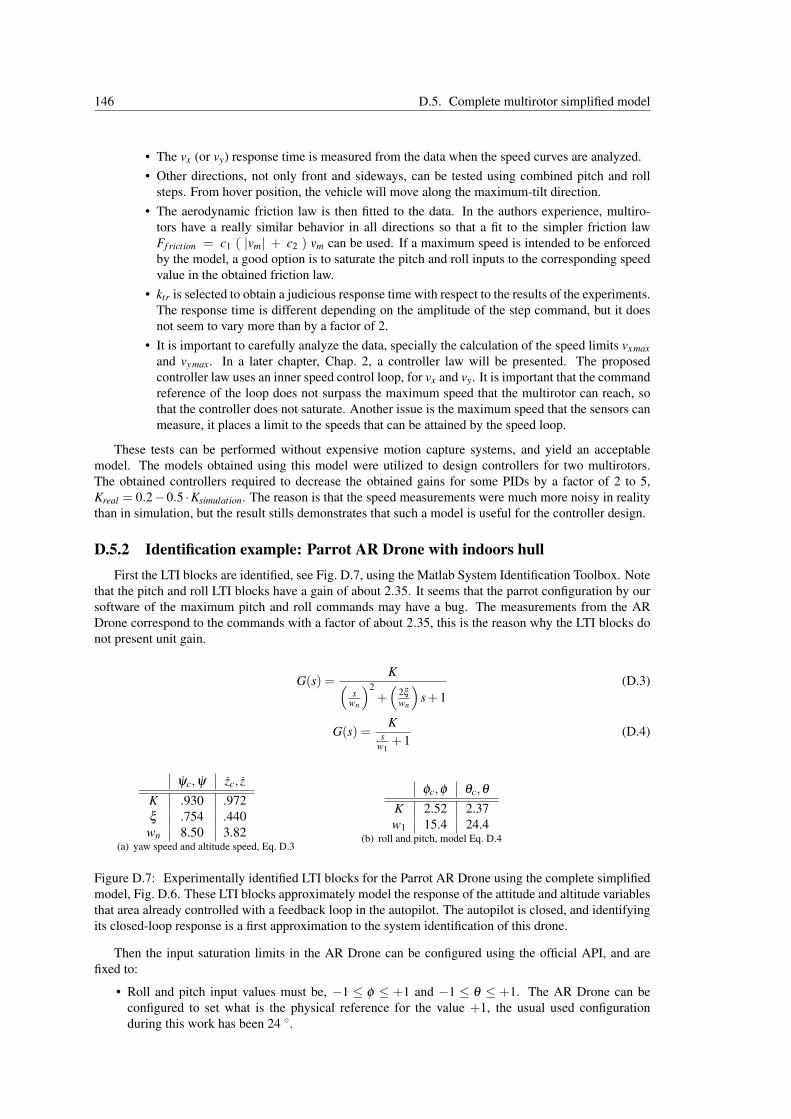
146 D.5. Complete multirotor simplified model
• The vx (or vy) response time is measured from the data when the speed curves are analyzed.• Other directions, not only front and sideways, can be tested using combined pitch and roll
steps. From hover position, the vehicle will move along the maximum-tilt direction.• The aerodynamic friction law is then fitted to the data. In the authors experience, multiro-
tors have a really similar behavior in all directions so that a fit to the simpler friction lawFf riction = c1 ( |vm| + c2 ) vm can be used. If a maximum speed is intended to be enforcedby the model, a good option is to saturate the pitch and roll inputs to the corresponding speedvalue in the obtained friction law.
• ktr is selected to obtain a judicious response time with respect to the results of the experiments.The response time is different depending on the amplitude of the step command, but it doesnot seem to vary more than by a factor of 2.
• It is important to carefully analyze the data, specially the calculation of the speed limits vxmaxand vymax. In a later chapter, Chap. 2, a controller law will be presented. The proposedcontroller law uses an inner speed control loop, for vx and vy. It is important that the commandreference of the loop does not surpass the maximum speed that the multirotor can reach, sothat the controller does not saturate. Another issue is the maximum speed that the sensors canmeasure, it places a limit to the speeds that can be attained by the speed loop.
These tests can be performed without expensive motion capture systems, and yield an acceptablemodel. The models obtained using this model were utilized to design controllers for two multirotors.The obtained controllers required to decrease the obtained gains for some PIDs by a factor of 2 to 5,Kreal = 0.2−0.5 ·Ksimulation. The reason is that the speed measurements were much more noisy in realitythan in simulation, but the result stills demonstrates that such a model is useful for the controller design.
D.5.2 Identification example: Parrot AR Drone with indoors hullFirst the LTI blocks are identified, see Fig. D.7, using the Matlab System Identification Toolbox. Note
that the pitch and roll LTI blocks have a gain of about 2.35. It seems that the parrot configuration by oursoftware of the maximum pitch and roll commands may have a bug. The measurements from the ARDrone correspond to the commands with a factor of about 2.35, this is the reason why the LTI blocks donot present unit gain.
G(s) =K(
swn
)2+(
2ξ
wn
)s+1
(D.3)
G(s) =K
sw1
+1(D.4)
ψc, ψ zc, zK .930 .972ξ .754 .440wn 8.50 3.82
(a) yaw speed and altitude speed, Eq. D.3
φc,φ θc,θ
K 2.52 2.37w1 15.4 24.4
(b) roll and pitch, model Eq. D.4
Figure D.7: Experimentally identified LTI blocks for the Parrot AR Drone using the complete simplifiedmodel, Fig. D.6. These LTI blocks approximately model the response of the attitude and altitude variablesthat area already controlled with a feedback loop in the autopilot. The autopilot is closed, and identifyingits closed-loop response is a first approximation to the system identification of this drone.
Then the input saturation limits in the AR Drone can be configured using the official API, and arefixed to:
• Roll and pitch input values must be, −1 ≤ φ ≤ +1 and −1 ≤ θ ≤ +1. The AR Drone can beconfigured to set what is the physical reference for the value +1, the usual used configurationduring this work has been 24 ◦.

Appendix D. Multirotor dynamics modeling 147
• The yaw speed is configured to uψ =+1command = 100 ◦/s = 1.745 rad/s
• The altitude speed is configured to uz =+1command = 1.0 m/s
Then several tests where performed in order to obtain the aerodynamic friction model. It is importantto note that all tests where done with the protective hull of the AR Drone. These tests were performedin a volleyball field that has a length of 18 m. The aerodynamic friction law was fitted using the MatlabCurve Fitting Toolbox, see Figs. D.8 & D.9.
(a) Pitch vs vx (b) Roll vs vy
Figure D.8: The figures show the average values of speed obtained in the aerodyncamic friction tests forthe Parrot AR Drone. Each graph correspondes to a different direction of movement: front movementusing step commands in pitch, and lateral movement using step commands in roll. The maximum speedobtained during tests was about 2.25 m/s, and for tilt values higher that 12 ◦ the speed was approximatelythe same and around 2 m/s.
Figure D.9: The figures show the average values of speed obtained in the aerodyncamic friction testsfor the Parrot AR Drone. Several datasets on the diagonal movement of the drone using step commandswith equal commands, φ = θ . The maximum speed obtained during tests was about 2.25 m/s, and fortilt values higher than 12 ◦ the speed was approximately the same around 2 m/s. The commands withtilt ≥ +1 were sent with the API, but probably the drone saturates this commands to +1.
The results for pitch step commands are shown in Fig. D.8(a) corresponding to frontal movement. Thefirst thing that stands out is that there is a part of the data that is linear, until pitch ≈ 0.5; but the rest ofthe graph shows that the steady-state speed is constant.
A possible explanation for this behavior is that for small angles the vehicle speed increases as thepitch increases. If the data is analyzed carefully the relationship is less linear as the angle increases, this isdue to the increasing surface area that the vehicle is showing in the direction of movement. This behavior

148 D.5. Complete multirotor simplified model
continues until at a specific angle, pitch, φ ≈ 12 ◦. A possible explanation is that at this point the flowaround the vehicle changes; causing that there is a maximum speed of about 2.25 m/s.
Data curves with similar characteristics where obtained for two more test directions: lateral and 45 ◦
diagonal directions. These curves are shown in Figs. D.8(b) & D.9.
(a) front direction (b) laterial direction
(c) diagonal direction (d) speed response for different step values
Figure D.10: Experimental identification of the aerodynamic friction law. The subfig-ures D.10(a) & D.10(b) & D.10(c) show the same data points as shown in Figs. D.8 & D.9,and also the curve that was obtained using data regression techniques with a funcion model:Ff riction = c1 ( |vm| + c2 ) vm. The subfigure D.10(d) shows the acquired speed measurements overtime for several of the step commands with different step values. A careful analysis of the curves insubfigure D.10(d) shows that the response time is about 3-4 s.
The subfigures D.10(a) & D.10(b) & D.10(c), shown in Fig. D.10, show the regression curves thatwhere used to fit the aerodynamic friction test data to the model Ff riction = c1 ( |vm| + c2 ) vm. TheMatlab Curve Fitting Toolbox was used to solve the regression problem. The values that were obtainedwere c1 = 0.0496 rad/(m/s) and c2 = 4.0 m/s, where c2 was fixed around the values obtained for threedatasets (one for each test direction). In the actual code, it is important to scale c1 by the gain of the pitchand roll LTI blocks, and c1 = 0.0496 ·2.35 rad/(m/s).
The last thing that was obtained from these tests was the response time of the horizontal speed in stepcommands tests. The obtained speed curves are shown in Fig. D.10(d), where several tests are shown.There are tests with different step values shown in the graph, but the response times remain approximately3-4 s, which corresponds to ktr ≈ 2.0 (adim).

Appendix D. Multirotor dynamics modeling 149
D.5.3 AR Drone model, comparison with experimental data
−2 −1 0 1 2
−4
−3
−2
−1
0
1Y
coord
inate
[m
]
X coodinatet [m]
vicon
model
Figure D.11: Comparison of AR Drone identified model to experimental data, X-Y trajectory. The shapeof the model’s trajectory is similar to the ground truth, the model estimates the loops in the waypoints ofthe trajectory. On the other hand, a lot of error is accumulated as the time passes.
It is important to compare the identified model with reality. As part of the development ofthe CVG Framework for interfacing with MAVs (Mellado Bataller, I., 2012; Mellado-Bataller etal., 2013), the author of the framework performed a test showing the viability of of the frameworkwith a trajectory controller. The AR Drone control problem was simplified using feedback infor-mation from a Vicon motion capture system, thus isolating the navigation problem from the local-ization/estimation problem. The video recorded during the test is available online in the websitehttps://www.youtube.com/watch?v=MFxfaHb7jT0. The data from the test offers: experimental input,telemetry and ground truth data (from the Vicon system). The availability of ground truth data for this testwas the main reason to use it as a comparison with the model implementation. The control during thistest was based on four PIDs: forward speed, lateral speed, yaw and altitude, which were adjusted from amodel estimation. The controller is a trajectory controller that follows a trajectory defined by waypoints.The feedback information required for navigation was obtained from a Vicon motion capture system.
The measurements are available with a common timescale and the data is divided in three sets:
1. Input data: {φ (roll), θ (pitch), ψ (yaw speed),−z (altitude speed)}
2. Telemetry data: the data that the AR Drone sends to the ground station which are the{φ roll, θ pitch, ψ yaw} coordinates, the altitude (from the sonar) and the {vxm, vym} speed esti-mations. The speed estimations are given in body frame coordinates (x, frontal direction, and y,lateral direction).
3. Ground truth localization dataset (Vicon): position and attitude data. The {x, y, ψ (yaw)} coordi-nates with respect to the world frame are compared with the model estimation.

150 D.5. Complete multirotor simplified model
In the following, several graphs are shown where the model data is either compared with the vicondata or the telemetry data. It is important to note that the model is only using the input dataset, nomeasurements are being used to increase the estimation quality. The take-off was eliminated from theestimation process, because the model did not perform well in that part; it estimated much higher speedsthan compared to reality. It was decided not to consider that part of the data for the analysis, for threereasons:
• the take-off mode of the AR Drone ignores the roll and pitch commands until the maneuver isfinished,
• it helps in the analysis task to work on data that corresponds to the conditions that the identificationprocess was aimed for,
• the take-off situation differs from the normal flying conditions and should be analyzed separately.
In general terms, the model behaves similarly to the system: the shape of the trajectory and the generalappearance of the curves in terms of rapidity/response time are comparable. However, it is clear from thehorizontal X −Y coordinates graph, Fig. D.11, that the position error increases gradually over time. Thisis expected as errors in the estimated velocities are integrated, resulting in the gradual increase of theposition error.
0 2 4 6 8 10 12 14 16 18 20
0.2
0.4
0.6
0.8
1
1.2
Vxm
[m
/s]
time [s]
telemetry
model
(a) Speed in body frame, frontal speed vxm
0 2 4 6 8 10 12 14 16 18 20
−1
−0.5
0
Vym
[m
/s]
time [s]
telemetry
model
(b) Speed in body frame, laterial speed vym
Figure D.12: Comparison of AR Drone identified model to experimental data, speed in body frame.The frontal speed estimation, vxm, is much more acceptable than the lateral speed, vym. The error in thelateral speed estimations makes the estimated trajectory shown in Fig. D.11, deviate to one side of theground truth. Both curves, estimated and telemetry, evolve similarly, with comparable response times.The take-off part of the simulation was not taken into account for the analysis and is not shown in thegraphs.
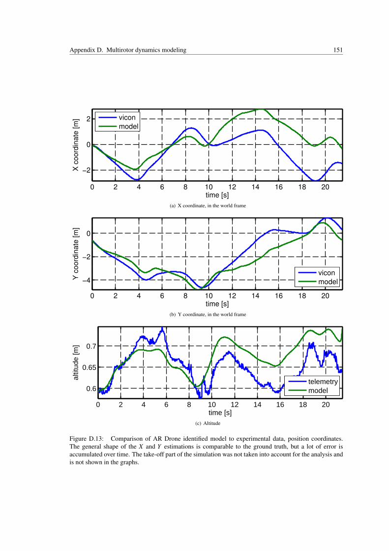
Appendix D. Multirotor dynamics modeling 151
0 2 4 6 8 10 12 14 16 18 20
−2
0
2
X c
oord
inate
[m
]
time [s]
vicon
model
(a) X coordinate, in the world frame
0 2 4 6 8 10 12 14 16 18 20
−4
−2
0
Y c
oord
inate
[m
]
time [s]
vicon
model
(b) Y coordinate, in the world frame
0 2 4 6 8 10 12 14 16 18 20
0.6
0.65
0.7
altitude [m
]
time [s]
telemetry
model
(c) Altitude
Figure D.13: Comparison of AR Drone identified model to experimental data, position coordinates.The general shape of the X and Y estimations is comparable to the ground truth, but a lot of error isaccumulated over time. The take-off part of the simulation was not taken into account for the analysis andis not shown in the graphs.

152 D.5. Complete multirotor simplified model
0 2 4 6 8 10 12 14 16 18 20−0.2
0
0.2
pitch [ra
d]
time [s]
telemetry
model
(a) Pitch angle
0 2 4 6 8 10 12 14 16 18 20−0.2
−0.1
0
0.1
roll
[rad]
time [s]
telemetry
model
(b) Roll angle
0 2 4 6 8 10 12 14 16 18 20−8
−6
−4
−2
0
Yaw
[ra
d]
time [s]
telemetry
model
vicon
(c) Yaw angle
Figure D.14: Comparison of the AR Drone identified model to experimental data, attitude angles. Thepitch estimation has an offset and it is noisy. The noise in the estimation is due to the control input, whichwas noisy for some reason (for instance, it could be a problem in the derivative part of the utilized PIDcontroller). The roll and the yaw estimation show good results. The take-off part of the simulation wasnot taken into account for the analysis and is not shown in the graphs.

Appendix D. Multirotor dynamics modeling 153
The speed estimation shows better results, Fig. D.12. The frontal speed, vxm, of the model has similaraverage value compared to the telemetry data. The laterial speed, vxm, is also similar, but the error is muchbigger. A really good characteristic of the model is that the curves in this figure have a similar appereance.Both curves seem to change smoothly, and present similar response times. The constant offset betweenthe commanded pitch and roll and its real values, see Fig. D.14, causes part of the estimation error invelocity.
The position coordinates {x, y} (with respect to the world frame) and the altitude are shown inFig.D.13. It can be seen again the similarity in the appereance of the curves. The estimation error isbig as commented before.
Finally, the attitude angles are shown in Fig. D.14. The pitch is much noisier than the roll estimation.This is probably due to differences in the frontal speed controller, and the lateral position controller;leading to the pitch command to be noisy. The roll estimation is good, and the pitch estimation presentsan offset with respect to the telemetry data. The yaw estimation is good and has little error.
It is interesting that during all the trajectory, the model estimation is oriented a little bit to the right,compared to the ground truth. This can be appreciated in the X −Y , Fig. D.11. The trajectory can bedivided in four segments, and comparing the corresponding segments between the estimation and theground truth; in three of them the model segment is deviated to the right with respect to the ground truth.The AR Drone was always oriented along the trajectory; with the heading parallel to the trajectory. It ispossible that the estimation error is due to an internal estimation offset in the roll and pitch angles.
D.5.4 Identification example: Asctec Pelican
ψc, ψ zc,zK 1.164 1.097ξ 1.398 .636wn 16.99 3.33
(a) yaw speed and altitude speed, Eq. D.3
φc,φ θc,θ
K 0.962 0.934w1 10.48 11.76
(b) roll and pitch, model Eq. D.4
Figure D.15: Experimentally identified LTI blocks for the Asctec Pelican using the complete simplifiedmodel, Fig. D.6. These LTI blocks approximately model the response of the attitude variables that areaalready controlled with a feedback loop in the autopilot. The altitude controller is implemented in theMAVwork framework.
First the LTI blocks are identified, see Fig. D.7, using the Matlab System Identification Toolbox.Then the input saturation limits in the Asctec Pelican can be configured using the CVG Framework forinterfacing with MAVs (Mellado Bataller, I., 2012; Mellado-Bataller et al., 2013). The values that wereused as saturation limits are:
• Roll and pitch input values are limited to 10 ◦.
• The yaw speed is configured for a maximum speed of 100 ◦/s.
• The altitude speed is configured to obtain a maximum of 1.0 m/s.
The aerodynamic friction tests where not performed for several reasons:
• A the moment our speed measurement system is a down-facing camera which images are processedusing optical flow algorithms. The optical flow is computed with the OpenCV implementation ofthe pyramidal Lucas-Kanade algorithm for some image features selected by the Shi-Tomasi method.The maximum speed that can be measured reliably at low altitude with this system was aroundvmeasurement,max = 0.75 m/s.
• The pelican was not well balanced at the moment, and it was difficult to stabilize it in hovering po-sition. Many tests ended because the vehicle was not moving in the correct direction but sideways,probably due to an offset in the commanded attitude angles internally controlled by the AsctecAutopilot.

154 D.5. Complete multirotor simplified model
• A the moment the developer team had the priority to participate in the IMAV 2012 competition.
As a summary, some tests were done and the following parameters were selected:
• For the aerodynamic friction law Ff riction = c1 ( |vm| + c2 ) vm, c1 = 0.1139rad/(m/s) and c2 =3.0 m/s
• The response time was about 4-6 s, and a value of 5 seconds was kept as response time. Then avalue of ktr = 1.317 (adim) was used.
The Asctec Pelican model has no been compared to ground thruth data, because no such data was avail-able.

Appendix D. Multirotor dynamics modeling 155
D.6 ConclusionsMore details on the identification methods and evaluations on real data of the described models can
be found in the MSc. thesis of the author Pestana, 2012, where these models were first presented. Themodels presented on this appendix have been used during the course of this PhD Thesis for the design of:
1. A speed, position and trajectory controller and an EKF for multirotors with an attitude controller ontheir Autopilot board. The EKF is used to estimate the position and velocity of the multirotor. Thecombined architecture has repeatedly allowed stable and precise quadrotor flight and our researchgroup has successfully used it and been awarded in its participation on various International MicroAerial Vehicle competitions, see Appx. I.
2. The design of an image based visual servoing controller, showcasing the capability of followingmany different targets using the low-cost AR Drone platform, see Chap. 3.
The main purpose of the discussed models was the design of reliable controllers for out of the lab au-tonomous flight, which was successfully achieved as demonstrated by the participation of the CVG_UPMin international MAV competitions and by the reliability of the developed visual-based object followingarchitecture.
However, more precise non-linear models have been identified successfully by other researchers dur-ing the course of this thesis. For the identification of the parameters of the rigid body dynamics basedmodel for multirotors the work by Achtelik et al. (Achtelik et al., 2013) is recommended. Also recentwork by other authors (Abeywardena et al., 2013; Leishman et al., 2014) have identified the horizontalaerodynamic friction on the propellers as a mayor force contributing to the dynamics of the multirotor andhave used this fact to derive improved estimation algorithms of the multirotor state.
156 D.7. Appendix Bibliography
D.7 Appendix BibliographyAbeywardena, D., Kodagoda, S., Dissanayake, G., and Munasinghe, R. (2013). “Improved State Esti-
mation in Quadrotor MAVs: A Novel Drift-Free Velocity Estimator”. IEEE Robotics & AutomationMagazine 20.4, pp. 32–39 (cit. on pp. 140, 155).
Achtelik, M. W., Lynen, S., Chli, M., and Siegwart, R. (2013). “Inversion based direct position controland trajectory following for micro aerial vehicles”. In: Intelligent Robots and Systems (IROS), 2013IEEE/RSJ International Conference on. IEEE, pp. 2933–2939 (cit. on p. 155).
Bristeau, P.-J., Callou, F., Vissiere, D., Petit, N., et al. (2011). “The navigation and control technologyinside the ar. drone micro uav”. In: 18th IFAC World Congress. Vol. 18, pp. 1477–1484 (cit. on p. 142).
Mellado Bataller, I. (2012). A new framework for interfacing with MAVs. https://github.com/uavster/mavwork (cit. on pp. 149, 153).
Fritsch, O., De Monte, P., Buhl, M., and Lohmann, B. (2012). “Quasi-static feedback linearization forthe translational dynamics of a quadrotor helicopter”. In: American Control Conference (ACC), 2012.IEEE, pp. 125–130 (cit. on p. 138).
Gillula, J. H., Huang, H., Vitus, M. P., and Tomlin, C. J. (2010). “Design of Guaranteed Safe ManeuversUsing Reachable Sets : Autonomous Quadrotor Aerobatics in Theory and Practice”. IEEE ElectricalEngineering (2010), pp. 1649–1654 (cit. on p. 139).
Hoffmann, Gabriel M, Waslander, Steven L, and Tomlin, Claire J (2008). “Quadrotor Helicopter Trajec-tory Tracking Control”. Electrical Engineering (2008), pp. 1–14 (cit. on pp. 138, 139).
Hoffmann, G.M., Waslander, S.L., and Tomlin, C.J. (2009). “Aerodynamics and control of autonomousquadrotor helicopters in aggressive maneuvering”. In: 2009 IEEE International Conference onRobotics and Automation. Ieee, pp. 3277–3282 (cit. on p. 140).
Leishman, R. C., Macdonald, J., Beard, R. W., and McLain, T. W. (2014). “Quadrotors and accelerom-eters: State estimation with an improved dynamic model”. Control Systems, IEEE 34.1, pp. 28–41(cit. on pp. 140, 155).
Mellado-Bataller, I., Pestana, J., Olivares-Mendez, M. A., Campoy, P., and Mejias, L. (2013). “MAVwork:a framework for unified interfacing between micro aerial vehicles and visual controllers”. In: Frontiersof Intelligent Autonomous Systems. Springer, pp. 165–179 (cit. on pp. 149, 153).
Michael, B. Y. N., Mellinger, D., and Lindsey, Q. (2010). “The GRASP Multiple Micro UAV Testbed”.IEEE Robotics & Automation Magazine, pp. 56–65 (cit. on pp. 138, 139, 141).
Pestana, J. (2012). “On-board control algorithms for Quadrotors and indoors navigation”. MA thesis.Spain: Universidad Politécnica de Madrid (cit. on p. 155).
Appendix EAn Extended Kalman Filter forMultirotors with Ground SpeedSensing
E.1 Introduction
For a mobile robot to navigate safely in any environment, it requires to have feedback about its ownmotion and about its localization. But multirotors and other rotary wing flying vehicles require informa-tion about their own speed to attain stabilization. This is an important difference between multirotors andother ground robots. A ground robot has some certainty about how to be in a stable position, and mea-suring the speed of its wheels gives a reliable speed measurement for this purpose. The direction of themovement can be commanded with a good level of certainty, and together with the speed estimation givesa somewhat reliable source of information. Its control algorithms can be based in the relative certaintythat is obtained from the speed measurements and of the effects of the commands on the movement of therobot to navigate. The robot still needs to localize to perform missions; but at least the robot can navigateslowly or stop moving when it is too uncertain of its localization or about nearby obstacles.
To the contrary, a multirotor has some uncertainty about its attitude. The problem is that little angleoffsets in the pitch or roll estimates, can lead to motion with a relatively high speed; easily of 0.5 m/s aftersome seconds. This means that if a speed controller with no reliable feedback has as objective to attainhover conditions, it can fail if it does not have reliable speed measurements. And more often than not,the vehicle is going to move at relatively high speeds. The attitude measurements alone are not enough tostabilize a multirotor. Multirotors can be in this situation for several reasons, for instance, if the weightis not well balanced the angle offset is aggravated. The consequence is that multirotors require goodself-motion feedback to attain reliable stabilization, in addition to the localization problem.
In multirotors the high-level (mission planning and supervision) and mid-level (speed, position andtrajectory control) control laws require a certain amount of accurate information about the quadrotor speedand position relative to the environment. This problem is not fully solved, but specific approaches give
157

158 E.2. State of the Art
an acceptable estimation for simplified environment models. For a detailed state of the art the reader isreferred to Sec. E.2.
The estimation and localization problem is really complex, some relevant bibliography about the prob-lem is (Koller et al., 2009; Rudy, 2003; Russell et al., 2003; Thrun, 2002). The measurements that areavailable for a robot can be classified as one of the following:
• The robot may have access to an a-priori known map describing the environment.
• The robot can use local navigation and measurements information to obtain his relative positionfrom a certain starting point. This gives rise to relative position measurements that are usuallyclassified as:
– Inertial: it involves using rotation speed and acceleration measurements from gyroscopes andaccelerometers. The IMU from a quadrotor uses both types of sensors to estimate the at-titude of the multirotor. However, this information is not enough to stabilize a multirotorautonomously.
– Odometry: essentially these are measurements related to the speed of the robot; with no ad-ditional localization information. The odometry measurements are integrated over time toobtain a relative position. The localization obtained has a good short-term accuracy, but theposition uncertainty increases over time. As explained before a multirotor requires odometryor relatively frequent position measurements to stabilize.
• Absolute position measurements supply information about the location of the robot with regards tothe environment and nearby obstacles; the location is not derived from integrating a sequence ofmeasurements, but directly from measurements that contain information about the robots relativeposition to nearby objects or from signals from beacons.
The methods to obtain absolute measurements can be divided into methods based on the use oflandmarks or beacons and methods based on the use of maps. Landmarks can be passive or active,depending on wether they actively send information to the robot or not. And maps can be geometricor topological: geometric maps describe the environment in metric terms, and topological mapsdescribe the environment in terms of characteristic features at specific locations and ways to getfrom one location to another. Both kind of maps can be known a priori by the robot, thus only havingto match sensor reading to the known map; or learnt while navigating through the environment. Themap learning task is known as SLAM (Thrun, 2002), Simultaneous Localization and Mapping, andit constitutes a very important and widely studied research topic.
This chapter is dedicated to explaining the filtering algorithms that have been implemented and suc-cessfully utilized during the course of this work. Sec. E.3, explains the filtering problem from a statisticalpoint of view introducing the state-observation model and the assumptions used by recursive filters, then,the Sec. E.3.1 is dedicated to general aspects of recursive filters. Sec. E.4, is dedicated to the KalmanFilter, with and explanation of the algorithm on Sec. E.4.1, and a brief explanation of the ExtendedKalman Filter on Sec. E.4.2. The equations of the complete multirotor simplified model are stated onSec. E.5, which was introduced in Appx. D.5. The experimental tests using the Kalman filter are shownin Secs. E.6 & E.6.1 & E.6.2. The Monte Carlo Localization is introduced in Sec. E.7, then the algo-rithm is explained in Sec. E.7.1; and a test of the implemented filter on experimental data is discussed inSec. E.7.2.
E.2 State of the ArtIn general terms, state estimation refers to the problem of calculating an estimate of the internal state
of the robot. It is interesting to understand this problem from a theoretical point of view, for instance asit is explained in the following two books: Artificial Intelligence: A Modern Approach (Russell et al.,2003), and Probabilistic Graphical Models: Principles and Techniques (Koller et al., 2009); and with amore experimental approach in the Msc. Thesis by Negenborn R., which gives a good insight into Kalmanfilters and other estimation algorithms applied to ground mobile robots (Rudy, 2003).
In order for a multicopter to, first, fly autonomously and, second, to take decisions, the robotic plat-form needs an accurate estimate of its position with regards to the environment. For the stabilization of
Appendix E. An Extended Kalman Filter for Multirotors with Ground Speed Sensing 159
the platform in the air, the mid-level control laws are provided with speed and position measurements,then enabling the position hold capacity to the multirotor. This basic operation is, for instance, interest-ing in maintenance operations of communication towers where the vehicle provides a close view of thecomponents of the tower.
The state estimation problem for multirotors remains an active research field, because dynamic ma-neuvers require fast and reliable estimates in the limited on-board hardware of the platform. However,specific approaches using Laser Range Finders (LRFs or lidars) give successful results for simplifiedenvironment models. In recent years, vision-based approaches are showing drastically improved results.
The environment model utilized by a robot limits the hazardous situations to which it can react suc-cessfully, thus limiting the commercial applications of mobile robots in unstructured environments. Forinstance, the ability to avoid an obstacle is limited by the type of obstacles that the robot can detect.Regarding the problem of indoors obstacle avoidance many previous work used a small number of ultra-sound or infrared sensors to attain basic obstacle avoidance in indoor environments (Bouabdallah, Samir,Murrieri, Pierpaolo, et al., 2005; Matsue et al., 2005; Roberts et al., 2007). Moving to the field of Com-puter Vision (CV), a camera can be used to classify the type of indoor environment where the MAV is in,and use this information to control the UAV based on perspective cues to estimate the desired directionto fly (Bills et al., 2011). However, more generally applicable solutions are required, such as real-timeSimultaneous Localization and Mapping (SLAM).
Inside buildings, a popular approach is the usage of laser range finders (LRFs) (such as theHokuyo URG-04LX-UG01) and lightweight implementations of SLAM algorithms. The following sur-vey by (Thrun, 2002) by Thrun S., gives an early introduction to the robotics SLAM problem. TheCSAIL MIT laboratory has used an Asctec Pelican quadrotor platform to explore unknown areas suc-cessfully (A. G. Bachrach, 2009; A. Bachrach et al., 2011). This areas would be similar to human-madeenvironments, were self-localization with respect to the lateral walls gives a good idea of the flyableobstacle-free space. The UAV used an stereo camera rig and an LRF to obtain the speed and positionmeasurements (A. Bachrach et al., 2011), and it was able to win the 2009 International Aerial Roboticscompetition (IARC2009), hosted by the Association of Unmanned Vehicle Systems Inter-national (AU-VSI); where the vehicle had to explore an environment made of hallways and rooms with little clutter,and locate a blinking device on a wall.
The GRASP laboratory of the Univesity of Pennsylvania has desmonstrated similar exploring capa-bilities 1 using a similar arrange of sensors with the Asctec Pelican (Shen, Michael, and Kumar, 2011).The vehicle was able to explore an unknown building with multiple floors, joining perfectly the obtainedmap whenever the vehicle came back to the same place through a new path. Later on (Shen and Michael,2013), the setup was improved to allow the UAV to fly changing from indoors to outdoors environments.The localization successfully switched to add GPS measurements to the state estimate 2. In a similarline collaborative mapping was also investigated, using a mobile robot along with the quadrotor (Michaelet al., 2012).
There are many industrial sites that are difficult to reach or hazardous for humans to enter, but they stillrequire inspection from time to time for routine or emergency reasons. An application research projectaimed to work on these conditions using an autonomous hexarotor was carried out at the Warwick MobileRobotics group (Abdul Shukor, 2013; Winkvist, 2013; Winkvist et al., 2013). As a motivation to thepossibilities of UAVs equipped with a LRF, the following are two demonstration videos of this projectwhere the UAV performs mapping during the a semi-autonomous flight: mapping of nuclear sites 3 and aflight demonstration 4.
The recent proliferation of cameras that provide depth along with the image, such as the MicrosoftKinect 5, has moved forward the field of processing point clouds in real-time. The Kinect and otherrelated sensors, use a hardware setup similar to an stereo camera, where one of the cameras is substitutedby an infrared projector that projects a pattern on the environment, which allows to perform triangulationwith the partner camera. A collaboration between the CSAIL lab of the MIT, and the Robotics and StateEstimation Lab (RSE-Lab) of the University of Washington gave as a result an Asctec Pelican quadrotorthat performed SLAM using a Kinect sensor. The so called RGB-D SLAM algorithm creates a 3D colored
1http://www.youtube.com/watch?v=IMSozUpFFkU , 20102https://www.youtube.com/watch?v=G_vtm46eGtU , 20123http://www.youtube.com/watch?v=Mz5z_xaB9i8 , 20114http://www.youtube.com/watch?v=w5tQ7iVJ4p8 , 20115http://en.wikipedia.org/wiki/Kinect , 2010

160 E.2. State of the Art
map of the environment (A. S. Huang et al., 2011). The paper from the RSE-Lab regarding this work isthe following (Henry et al., 2010).
In the last years there has been an increasing potential of computer vision based algorithms. Thefollowing study, on the performances of vision based point cloud algorithms versus their LIDAR (LRF)based counterparts (Leberl et al., 2010), shows that computer vision bundle adjustment methods are, since2010, cost-effective and obtain better results. The study is based in two practical examples comparingpoint clouds created from LIDAR systems and from images: aerial surface mapping and street mapping.In general terms the image based methods have an accuracy comparable to LRFs, but they offer a higherpixel density, meaning that more points are reconstructed per unit surface. Regarding this topic, thereference book to introduce the relationships between image points on images of the same scene is thebook Multiple View Geometry in Computer Vision, (Hartley et al., 2004).
One of the first works that achieved a real-time SLAM algorithm based on vision, and that was able toperform real-time robot exploration was the thesis by Andrew Davidson (A. J. Davison, 1998), which wasdemonstrated using a ground robot. The approach uses an algorithm that is able to recognize new featuresof the scene that can be located repeatedly from different viewpoints. An EKF is used to filter the dataand obtain the camera position with respect to the environment, the estimated position of the features isadded as part of the state representation of the filter. This work gave way to more improvements (Moltonet al., 2004) and applications , for example the development of a wearable camera that interacts with theuser to highlight objects in the scene (Mayol et al., 2004).
In recent research, new approaches to the visual SLAM problem showed much better results than thefiltering or EKF approach, both in terms of computation efficiency and accuracy. George Klein et al.designed a new localization algorithm (Klein et al., 2007) called Parallel Tracking and Mapping (PTAM)for Augmented Reality applications. The algorithm first required the computing power of a laptop, buttwo years later was able to make it work on an iPhone (Klein et al., 2009). Further works by the group ledby Davidson studied the advantages of PTAM over the former filtering-based algorithms (Strasdat et al.,2010), explaining the reasons for its better performance. An improved version of PTAM was designedby this group, and was called Live Dense Reconstruction (DTAM) (R. A. N. Davison et al., 2010). Thisnew algorithm uses not only salient points and image features, but also the texture of potentially allpoints in the image, to perform the localization calculations. DTAM has been shown to be stable andvery precise in more difficult conditions: fast camera movements and camera defocusing among others6. The approach was to include more pixel information on the map by combining the current cameraposition estimations with dense optical flow techniques. However, PTAM has been preferred in the UAVcommunity, first because is available as open-source software for research, and second because it has lesscomputing requirements, which allows to run it on-board an UAV.
The PTAM algorithm was widely used in the sFly project 7. First results, showed how to fuse themeasurements from the IMU with the output of the PTAM algorithm (Nützi et al., 2011), based on theusage of an Extended Kalman Filter (EKF). Later results, showed autonomous flight performance inoutdoors environments and scale recovery of the PTAM reconstructed map (M. W. Achtelik, Lynen, S.Weiss, et al., 2012; S. Weiss, M. W. Achtelik, Lynen, et al., 2012). The following paper summarizesthe research contribution of the sFly project, in terms 3D Mapping, collaborative mapping and of visual-inertial fusion for state estimation and control of multirotors (Scaramuzza et al., 2013). The latter has beenpartially released as open-source software 8, which can work in a low-end on-board computer. Related tothis works, there are two other software repositories which are designed to perform a visual-inertial basedstate estimation for multicopters by fusing the output of PTAM, IMU measurements, and other sensors.They are the result of multiple consecutive works (Lynen et al., 2013; S. M. Weiss, 2012; S. Weiss,M. W. Achtelik, Chli, et al., 2012; S. Weiss, Scaramuzza, et al., 2011; S. Weiss and Siegwart, 2011) andhave resulted in two popular open-source repositories 9 10. Another influencing research on fusing IMUmeasurements with the output of PTAM was performed by Jakob Engel et al. in 2012 (Engel, Jakob et al.,2014; Engel et al., 2012), and is also available as an open-source package 11. The main difference betweenboth works is that the latter was realized using an off-board computer, since the flying platform is an AR
6 https://www.youtube.com/watch?v=Df9WhgibCQA , 20117http://www.sfly.org/ , Swarm of Micro Flying Robots (FP7/2007-2013)8http://wiki.ros.org/asctec_mav_framework , 20129http://wiki.ros.org/ethzasl_sensor_fusion, 2012
10https://github.com/ethz-asl/ethzasl_msf, 201211https://github.com/tum-vision/tum_ardrone , 2012

Appendix E. An Extended Kalman Filter for Multirotors with Ground Speed Sensing 161
Drone, and that the scale of the map is recovered in a different manner. PTAM has also been explored asa technique to perform collision avoidance in indoors environments for wall-like obstacles in (Fu et al.,2013).
The Aerial Vision Group of the Institute for Computer Graphics and Vision of the Graz University ofTechnology (Wendel, Maurer, et al., 2011) is applying several 3D vision techniques to images acquiredby quadrotors. Both for reconstruction purposes and for localization. A localization technique based onthe PTAM algorithm for multirotors was developed in (Wendel, Irschara, et al., 2011). The techniquerequired to obtain a 3D map of the environment from hand-held camera images. The map was specificallydesigned to be able to locate the camera. Their work often applies the concept of vocabulary trees (Nisteret al., 2006) to asses the identification of the same image point in several images. The algorithm has theadvantage of being able to manage larger feature databases, by relating them if they appear together inseveral images. The vocabulary tree algorithm has its origins on web crawlers and web-page indexingalgorithms.
New advancements in vision-based SLAM have been done since the development of PTAM andDTAM. For instance, a collaborative SLAM approach performed by multiple multicopters (Forster, Ly-nen, et al., 2013). But more interestingly, two outstanding new algorithms that are based on direct-visionmethods, which means that they do not employ image features, are the LSD-SLAM algorithm12 fromJakob Engel et al. (Engel, Schöps, et al., 2014; Engel et al., 2013) from the TU Munich Computer Visiongroup; and the SVO algorithm13 by Christian Forster et al. (Forster, Pizzoli, et al., 2014) from the ETHZurich Robotics & Perception Group. As their names suggest, one of them is a full SLAM method, andthe other is a Visual Odometry one, both have in common the requirement that the image streams need tohave a high frame-rate; so that the tracked points do not experience a big displacement between frames.However, they can both run on hardware with limited computing power. Both of these algorithms areprobably going to inspire much research, in the same way that PTAM has done in the past.
It is also outstanding the highly optimized visual-inertial odometry pipeline developed by ShaojieShen et al. (Shen, Shaojie et al., 2013; Shen, Mulgaonkar, et al., 2013) at the GRASP Laboratory ofthe University of Pennsylvania. In comparison to SVO, the pipeline is featured-based; but leveragesIMU integration, carefully selected fast CV algorithms that decouple rotation from translation estima-tion (Burschka et al., 2008) and the utilization of Unscented Kalman Filters (Julier et al., 1995; NøRgaardet al., 2000; Wan et al., 2001). This pipeline has been demonstrated to be able to perform real-time stateestimation while flying and being executed in a low-end on-board computing platform, on a board with atwo-core Atom processor computer. In the same line of visual-inertial fusion, it is very remarkable the ac-complishment of fusing IMU measurements with visual based ones jointly in a SLAM bundle adjustmentoptimization framework by Stefan Leutenegger et al. (Leutenegger, Furgale, et al., 2013; Leutenegger,Lynen, et al., 2014) from the ETH Zurich. Additionally, this works are complemented by the devel-opment of a commercially available Visual-Inertial Stereo camera sensor, that efficiently synchronizesIMU measurements and the image acquired data (Nikolic et al., 2014), and also by a the new Binary Ro-bust Invariant Scalable Keypoints (BRISK) descriptor (Leutenegger, Chli, et al., 2011); which performssimilarly to more computationally intensive descriptors but that is orders of magnitude faster. Althoughshowing that this algorithm can run on real-time on limited computing hardware is still to be done, it isoutstanding that it is the first algorithm of its class, and it may give way to a new family of algorithmsthat can optimally fuse visual-based measurements with data gathered from other sensors using BundleAdjustment (BA); which has usually been done in the past using EKF or related frameworks.
Probably one of the best exponents of EKF based visual-inertial fusion are the works by Mourikis etal. (Mourikis and Roumeliotis, 2006; Mourikis and Roumeliotis, 2007), which developed the so-calledMulti-State Constraint Kalman Filter (MSCKF). A slightly modified version of this algorithm was shownto be able to drastically improve the accuracy of the localization of an spacecraft entry and landing oper-ation, which was simulated acquiring real data during a sounding rocket experiment (Mourikis, Trawny,et al., 2009). The MSCKF algorithm has been improved during the years still with the participationof Mourikis (Li et al., 2013), and many interesting issues have been tackled: like an approach to dealwith rolling-shutter cameras during SLAM (Li et al., 2014b), and works regarding the on-line temporalcalibration of visual and inertial measurements (Li et al., 2014a).
12Large-Scale Direct Monocular SLAM (LSD-SLAM), released as open-source in GitHub https://github.com/tum-vision/lsd_slam , 2014
13Fast Semi-Direct Monocular Visual Odometry (SVO), released as open-source in GitHub https://github.com/uzh-rpg/rpg_svo , 2014

162 E.2. State of the Art
After discussing recent advances in localization estimation techniques, the discussion is here focusedagain on the topic of multicopters. Mapping, potentially recognizing obstacles to be avoided and localiz-ing the drone with respect to the environment are critical robotic tasks; but what state is otherwise neces-sary to estimate, to attain a competitive flight control, will be now discussed. Of the control approachesused with quadrotors, it is interesting to address this topic from the ones that exploit the differentialflatness of quadrotor flight. A system is differentially flat if there exists a set of outputs from it whichfully determine the state of the system given the values of the flat outputs and their derivatives (to a givenorder)14 (Fliess et al., 1995; Murray et al., 1995). When a non-linear system is differentially flat, this char-acteristic can be used for both: control and trajectory generation (Dunbar et al., 2003; Van Nieuwstadtet al., 1998). This concept is of great interest for multicopters, since they are highly non-linear dynamicsystems. The characteristic that they are differentially flat was demonstrated and shown by Mellinger etal. in (Mellinger et al., 2011). This fact has allowed the development of very competitive control (Fritschet al., 2012) and trajectory generation algorithms (Mellinger et al., 2011; Richter et al., 2013) for theseplatforms. By the property of differential flatness, and as exploited by the two latter cited papers, the stateof the quadrotor can be fully determined by its linear position, speed, acceleration, jerk and jounce (orsnap); and by its yaw rotation, speed and acceleration (Mellinger et al., 2011). This means, that besideslocalization and mapping, it is desirable for multicopter control to determine its position, speed, accel-eration; attitude and rotation speed; and possibly more of their derivatives, until the orders mentionedabove.
In terms of multicopter model identification, there are many unknowns to be determined: mass, mo-ments of inertia, thrust and torque constants of the propellers, etc. The full quadrotor model identificationscheme introduced by Markus Achtelik et al. (M. W. Achtelik, Lynen, Chli, et al., 2013), which waspartly motivated by prior work in the ETHZ Flying Arena (Schoellig et al., 2012), can be used for systemparameter estimation purposes and is able to determine the subset of them that is absolutely necessary toperform dynamics inversion based control.
In terms of attitude estimation, the issue is that competitive attitude estimators are a research topicby themselves. There are many different mathematical attitude representation methods (Shuster, 1993).Quaternions are probably the preferred rotation representation method (Kuipers, 2002), because of theirlack of singularities and minimal number of parameters, but care must be taken to know which quaternionconvention is used. There are two main conventions: the Hamilton convention and the JPL conven-tion (Breckenridge, 1999), which is for instance used in this attitude estimation paper (Trawny et al.,2005). A neat explanation of quaternion conventions is given in this technical report by Joan Solà (Sola,2012), which might be used in combination with these papers (Barfoot et al., 2011; Trawny et al., 2005)to understand the linearization of the state error of attitude states when represented by quaternions. Thusas a first step, it is very important to know which convention is used in a given paper or software library.Then, there are multiple attitude estimation methods that have been already tested. The following workpresents a detailed summary of non-linear observers (Misawa et al., 1989), and a more modern overviewof attitude estimation methods is presented in (Crassidis et al., 2007). The conventional way of performingattitude estimation is based on the Extended Kalman Filter (EKF) algorithm (Farrell, 1970; Lefferts et al.,1982; Schmidt, 1981), and the Multiplicative Extended Kalman Filter (MEKF) (Markley, 2003; Murrell,1978). Popular attitude quaternion estimators are presented in (Shuster and Oh, 1981) and (Psiaki, 2000).The Unscented Kalman Filter (UKF) (Julier et al., 1995; NøRgaard et al., 2000; Wan et al., 2001) canbe also used for attitude estimation and it is based on performing second order or higher approximationsof the non-linear system; which differs from the EKF that is based on a first order approximation. How-ever, many of the afore mentioned methods still put constraints on the probability density function of thetracked system. A popular estimation approach which does not make any such assumptions is the ParticleFilter or Monte Carlo Method (Arulampalam et al., 2002; Doucet et al., 2001), which has been applied toattitude estimation in the following works (Cheng et al., 2004; Oshman et al., 2004).
Currently, there are three quadrotor open-source quadrotor simulators based on the Gazebo 3D rigidbody simulator for robots, the first was developed by Meyer et al. (Meyer et al., 2012) from TU Darmstadt15 , and the second is an adaption from the first by Hongrong Huang et al. 16 to simulate an AR Drone1.0 or 2.0 quadrotor. The third, the RotorS simulator framework (Furrer et al., 2016), was utilized by
14http://en.wikipedia.org/wiki/Flatness_%28systems_theory%29 , 201515https://github.com/tu-darmstadt-ros-pkg/hector_quadrotor , 201216https://github.com/tum-vision/tum_simulator , 2013

Appendix E. An Extended Kalman Filter for Multirotors with Ground Speed Sensing 163
the EuRoC201417 organizers during the simulation challenge. The main feature of the RotorS simulatorare that it utilizes the Gazebo physics engine, that it can be easily run and interfaced using ROS, that itprovides a controller and a state estimator to help the user getting started, and that it provides an alreadyimplemented evaluation framework. Comprehensive models for quadrotors can be found in many papers,but the two following are highlighted, the hector_quadrotor simulator paper (Meyer et al., 2012), and themulticopter parameter identification described in the following paper by Markus Achletik et al. (M. W.Achtelik, Lynen, Chli, et al., 2013). Previous works by the STARMAC project, a quadrotor projectthat took place at the Standford University, describe aerodynamic considerations that should be takeninto account by multicopter models (Hoffmann et al., 2007; H. Huang et al., 2009). A quadrotor modeldeveloped for the open-source FlightGear flight simulator is described in (Goel et al., 2009). And a modelthat includes many aerodynamic effects present in quadrotors was introduced in (Bouabdallah, Samir andSiegwart, Roland, 2007).
However, a very important aspect that is often not described, is the mathematical modeling of theinertial sensors themselves. The MSc thesis by Minha Park was focused on determining the sources ofmeasurement error in MEMS (Microelectromechanical systems) based inertial sensors (Park, 2004). Gy-roscopes measure the rotational speed of a rigid body with respect to an inertial frame, and are affectedby noise and by a time varying drift. More concise works which give the mathematical model represen-tations for gyroscope sensors are provided in (Abeywardena et al., 2013; Crassidis, 2006; Farrenkopf,1978). Accelerometers measure the specific acceleration of a body, which means that they measure theacceleration of the body minus the gravity. Thus, in order to exploit their measurements, it is desirableto use a model that takes into account most, if not all, of the forces acting on the quadrotor body. Thus,the model should include aerodynamic forces among others, and this fact has been the target of recentresearch (Abeywardena et al., 2013; Leishman et al., 2014) which have demonstrated that the inclusion ofsuch forces increases the overall performance of the multicopter state estimator. The authors achieved thisby identifying the friction on the propellers of the multicopter as a mayor contributor to the aerodynamicfriction of the aircraft (Leishman et al., 2014).
E.3 Dynamic systems and filtering algorithms
There are two sources of information that a robot can exploit to navigate, see (Koller et al., 2009; Rudy,2003; Russell et al., 2003; Thrun, 2002). The first, is the commands it is sending to its engines or actuators.For example, a multirotor could use the rotor speed references it is sending to the ESC boards, to simulateits rigid body dynamics, see Appx. D.2. The second, is that the robot can use sensor measurements tocorrect the estimation of his self-motion. Both information sources are available frequently over time, ina discrete manner.
In order to reason mathematically about the motion of a robot, and be able to implement estimationalgorithms; it is important to have a dynamic stochastic model of the robot. The model encodes manyinformation about the system. For instance, the minimum required frequency of arrival of measurementsand commands to the estimation module can be determined from the model. As a specific example, ifthe horizontal speed of a multirotor shows a response time of 3 seconds, then the minimum frequencyrequired for the speed measurements is about 1
3 s/5 ≈ 1.7 Hz.The dynamics model, also called a State-Observation model, of the robot has the following elements:
• Xt : a set of state variables that among other things, represent the position, speed and orientation ofthe robot. Part of these variables may be measured but always with a varying level of uncertainty.‘t’ denotes the time variable.
• Ut : is the set of command variables that are sent to the engines of the robot.
• Ot : denotes the set of measurements
• A transition model that specifies how the state of the robot may evolve. It is usually specified as anstochastic relationship P(Xt+1 |X1:t ,U1:t), between the previous values of the state and the currentcommand Ut .
17http://www.euroc-project.eu/

164 E.3. Dynamic systems and filtering algorithms
• A observation model that specifies the probability distribution of the measurements depending onthe state P(Ot |X1:t , O1:t−1).
The term P(Xt |X1:t ,U1:t) is called belief state, and it containts the probability distribution of Xt takinginto account all the prior information about the system’s trajectory. It is important to note that it potentiallydepends on all the past values of the variables at the right. The problem is that the past values of the stateand commands can grow unboundedly over time. This problem is usually solved making the ‘Markovassumption’, which basically states that the current state of a dynamic system depends only in a finitefixed number of previous states and commands. The simpler version of the assumption is the first-orderMarkov process which states that the current state depends only on the previous state and command:
P(Xt+1|X1:t ,U1:t) = P(Xt+1|Xt ,Ut) (E.1)
This equation is further simplified assuming “time invariance”, that is, that the robot is governedby model equations that do not themselves change over time. Both hypothesis are also applied to theobservation model, obtaining:
P(Ot |X1:t , O1:t−1) = P(Ot |Xt) (E.2)
The type of inference problems that can be solved using the dynamic model of the robot are:
• Filtering: it is the task of computing the belief state (the posterior distribution over the most re-cent state) given all the evidence to date. With the prior notation this would involve calculating,P(Xt+1|O1:t ,U1:t).
• Prediction: this is the task of computing the posterior distribution over the future state, given allevidence to date. That is, to calculate P(Xt+k|O1:t ,U1:t) for k ≥ 0.
• Smoothing: this is the task of computing the posterior distribution over a past state, given all evi-dence up to the present. That is, to compute P(Xk|O1:t ,U1:t) for some k such that 0≤ k < t.
• Most likely explanation: given a sequence of observations, we might wish to find the se-quence of states that is most likely to have generated those observations. That is, to calculateargmaxX1:t
P(X1:t |O1:t ,U1:t)
A useful filtering algorithm needs to maintain a current state estimate and update it, rather than goingback over the entire history of measurements for each new update. Otherwise, the cost of each updatewould increase as time goes by. A filtering algorithm with this property is called a recursive filteringalgorithm. This means that it is necessary that given the posterior distribution P(Xt |O1:t ,U1:t) and thenew measurement Ot+1 the algorithm must be able to calculate
P(Xt+1|O1:t+1,U1:t+1) = f (Ot+1, P(Xt |O1:t ,U1:t)) (E.3)
Note the requirement to only use the posterior distribution and the new measurement, this is reallyimportant because it permits to decrease the memory requirements of the algorithm.
E.3.1 Filtering in State-Observation modelsFocusing on the filtering of the dynamic system state, there exists an approach that provides a simple
recursive rule for the filtering problem. The Markovian assumption underlying the State-Observationmodel provides a recursive two step approach that relies only in the posterior distribution P(Xt |O1:t ,U1:t)and the new measurement Ot+1 to calculate P(Xt+1|O1:t+1,U1:t+1). The two steps are the following:
First there is a prediction step, that uses the state estimation and the command input to predict thestate at the moment of arrival of the measurement:
P(Xt+1|O1:t ,U1:t) = ∑Xt
P(Xt+1|Xt , O1:t ,U1:t) P(Xt |O1:t ,U1:t)
(Markov assumption) = ∑Xt
P(Xt+1|Xt ,Ut) P(Xt |O1:t ,U1:t) (E.4)

Appendix E. An Extended Kalman Filter for Multirotors with Ground Speed Sensing 165
Note that the transition model of the system is used as part of this step. This step can be understood as aconvolution of the posterior probability at t and the transition model to predict the state at t +1, that canbe called prior belief state.
The first step is repeated over time whenever a state estimation is required by some module of thesystem. Then, when a measurement is available, the prior belief state is conditioned on the measurementto update the state estimation:
P(Xt+1|Ot+1, O1:t ,U1:t) =
(Bayes Rule) =P(Ot+1|Xt+1, O1:t ,U1:t) P(Xt+1|O1:t ,U1:t)
P(Ot+1|O1:t ,U1:t)
(State-Observation model) =P(Ot+1|Xt+1) P(Xt+1|O1:t ,U1:t)
P(Ot+1|O1:t ,U1:t)(E.5)
This simple recursive filtering procedure maintains the belief state over time, without keeping track ofa network or a sequence of observations of growing length. This characteristic reduces both the memoryrequirements of the algorithm and also the number of computations to propagate the belief state over time.
This two-step process is used in the two approaches that are explained in this chapter: the KalmanFilter (KF), and the Particle Filter (PF).
As it will be explained in Sec. E.4, the Kalman Filter performs the calculations steps in Eqs. E.4 & E.5making the assumption that all the variables (measurements, inputs and state) can be modeled as Gaussiandistributions. It is important to note that the acceptance of this assumption depends on the quality of themodel. If the model explains well enough the internal dynamics of the system, then it is probable thatthe relationship between the state variables can be modeled with Gaussians. The Kalman Filter has thelimitation that it works only with unimodal distributions, which can be a limitation in some situations.
On the other hand, the Particle Filter, Sec. E.7, implements the Eqs. E.4 & E.5 using sampling meth-ods. The algorithm maintains a population of particles that is updated overtime using these equations.Its main advantages are that it is easy to implement and it is easy to incorporate new sensors to the im-plementation. It is specially well prepared to work with sensors such as laser range finders. And a bigdifference with the Kalman Filter is that it can maintain multimodal distributions. In the case where themeasurements are ambiguous, the population is divided between the possible sources of the measurementuntil new measurements and navigation data clarify which population is the correct one.
E.4 Kalman filterThe Kalman Filter (KF) is a recursive data processing algorithm that has successfully been used in
a wide range of applications and specifically in many artificial intelligence and robotics problems. Forinstance, it can be used as a sensor data fusion algorithm in the IMU of a multirotor that combines themeasurements from the gyroscopes, accelerometers and magnetometer together.
The KF, as a recursive filtering algorithm, can be understood as an implementation of the two stepprediction-correction algorithm explained before, see Eqs. E.4 & E.5. The State-Observation model ex-plained in Sec. E.3 is stochastic and includes uncertainty in both the transition and the observation models.It is important to note that the uncertainty is specified adding white noise stochastic variables in the equa-tions of the model. Then, these noise variables are defined with different variance values to account forthe different levels of uncertainty.
In the measurement update step, Eq. E.5, the KF compares the uncertainty of the state estimation andthe measurements, and combines both distributions to minimize variance of the state estimation error.During the propagation over time of the belief state using Eq. E.4 the uncertainty increases gradually dueto the presence white noise in the model. And in the measurement step, the uncertainty is reduced again,providing a mechanism to bound and minimize the uncertainty of the estimation over time.
The variance values of the noise variables are selected, first taking measurements about the concernedparts of the system. This can lead sometimes to a KF that relies to much either on the measurementsor in the transition model. Therefore, the variance values are further tuned to obtain a somewhat optimalfiltering behavior. This is important, because in many robotic problems the KF is used to provide feedbackto a controller, and a good tuning of these parameters leads to a more preferable navigation behavior ofthe robot.

166 E.4. Kalman filter
E.4.1 The Kalman Filter algorithmThe KF is based on a number of hypothesis on the system, measurements and different noises that are
involved in the estimation problem. The KF assumes that the system is adequately modeled by a lineardynamic system:
Transition model: xt = Axt−1 +But−1 +wt−1 (E.6)Observation model: zt = Hxt +νt (E.7)
where,
• The true state of the system xt depends on the previous state xt−1 trough the state matrix A, thecommand in the previous state ut−1 trough the command matrix B, and the state noise wt−1.
• The state noise is a Gaussian white noise, wt ∼N (0, Qt)
• The command is stochastic with mean ut , ut ∼N (ut ,Ut)
• The true measurement zt depends linearly on the state at time t, xt , trough the observation matrixH. The uncertainty in the measurement is modeled through the measurement noise νt .
• The measurement noise νt is a Gaussian white noise, νt ∼N (0, Rt)
The noise variables are independent from one another, white, Gaussian and with zero-mean. Moreover,the KF assumes that an estimate of the initial state of the system is available and that it can be representedwith an independent Gaussian distribution.
x0 ∼N ( x0, P0) (E.8)
The Kalman Filter starts with an initialization step after which it alternatively performs prediction andcorrection steps. The algorithm itself is described in the following:
Initialization:The filter is initialized with an estimated state, x0, and a state estimation error covariance, P0.
Prediction equations:If the equation E.4 is implemented using the state-observation model introduced before, then the followingequations are obtained:
x−t = Ax+t−1 +But−1 (E.9)
P−t = AP+t−1AT +BUt−1BT +Qt−1 (E.10)
The set, { x−t+1, P−t+1}, consisting of the state and the state covariance matrix at t +1 is called prior beliefstate. This step can be performed multiple times until a new measurement is acquired. As stated before,the uncertainty over the state estimation increases over time. The correction step bounds the variance ofthe estimation by means of the comparison of the uncertainties of the belief state and the measurements.
Correction equations:The correction or the measurement update equations use the new measurement to update the state estimate.The measurements give information about the current state of the system. The correction equation are aversion of Eq. E.5 adapted to the Kalman Filter hypothesis:
x+t = x−t +Kt(zt −Hx−t
)(E.11)
P+t+1 = (I−KtH)P−t (E.12)
Kt = P−t HT (HP−t HT +Rt)−1
(E.13)
First the measurement innovation,(zt −Hx−t
), is calculated. Then the uncertainty of the prior belief and
from the measurement are compared to calculate the strength, Kt , with which the innovation is used toupdate the state estimate, x+t , and the estimation covariance, P+
t+1.The new posterior belief is used in the next time step to compute the new prior belief. This recursive
nature of KFs allows for practical implementations, because not all of the data is required to estimate thestates. Also note that the filter can be used with multiple asynchronous measurement update frequencies.

Appendix E. An Extended Kalman Filter for Multirotors with Ground Speed Sensing 167
When the filter has much more confidence in the model than in the measurements, then Kk ≈ 0, andthen x+t ≈ x−t +0, P+
t+1 ≈ P−t . To the contrary, when the filter overestimates the uncertainty of the model,then Kk ≈H−1
t , and then x+t ≈H−1t zt . These two last equations are too simplified and only apply on same
cases where all the states are measured.In short, the KF calculates the belief state by performing two alternating steps:
• In the prediction step the KF calculates the prior belief. This belief consists of the prior stateestimate and the prior error covariance, which describes the uncertainty in the state estimate. Giventhe model and the last state estimate the prediction step predicts the most likely current state of thesystem after a time step.
• The KF applies the correction step when it has access to a measurement. It uses the measurement toform the posterior belief. The KF computes the measurement innovation as the difference betweenthe true measurement and a measurement prediction. It uses the kalman gain to determine to whatextent the measurement innovation should be incorporated into the state estimate.
E.4.2 Extended Kalman FilterThe EKF is an extension of the KF to the case where the model dynamics are non linear:
Transition model: xt = f (xt−1, ut−1)+wt−1 (E.14)Observation model: zt = h(xt)+νt (E.15)
where the state matrixes are derived from the model trough derivation:
At =∂ f∂x
∣∣∣∣xt
(E.16)
Bt =∂ f∂u
∣∣∣∣ut
(E.17)
Ht =∂h∂x
∣∣∣∣xt
(E.18)
The algorithm follows the same steps as the KF, but utilizes the first-order approximation of the modelaround the current belief state at t:
Initialization:The filter is initialized with an estimated state, x0, and a state estimation error covariance, P0.
Prediction equations:If the equation E.4 is implemented using the state-observation model introduced before, then the followingequations are obtained:
x−t = Ax+t−1 +But−1 (E.19)
P−t = AP+t−1AT +BUt−1BT +Qt−1 (E.20)
At =∂ f∂x
∣∣∣∣x+t−1, ut−1
Bt =∂ f∂u
∣∣∣∣x+t−1, ut−1
Correction equations:The correction equation are the version of Eq. E.5 adapted to the Kalman Filter hypothesis:
x+t = x−t +Kt(zt −Hx−t
)(E.21)
P+t+1 = (I−KtH)P−t (E.22)
Kk = P−t HT (HP−t HT +Rt)−1
(E.23)
Ht =∂h∂x
∣∣∣∣x−t
The Jacobian matrices Ak and Hk are evaluated at the most recent state estimates. Since the stateestimates are not known in advance, the Jacobians can not be computed off-line as is the case with theKF. Thus, in the EKF case, the Jacobians have to be computed on-line, resulting in higher computationalcosts.
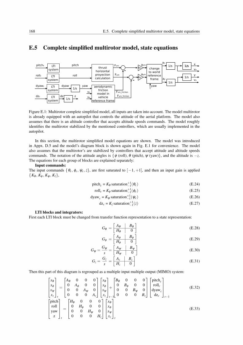
168 E.5. Complete simplified multirotor model, state equations
E.5 Complete simplified multirotor model, state equations
pitch
vx
LTIsystem
1/s
vy
1/s
x
y
aerodynamicfriction
model in vehicle
reference frame
pitchc
rollLTIsystem
rollc
dyawLTIsystem
dyawc1/s
yaw
dzLTIsystem
dzc1/s
z
thrust horizontal proyection calculation
ktr
ktr
changeto world
referenceframe
vx
vy
Fxm_friction
Fym_friction
Fxm
Fym
1/s1/s
1/s
-
-
axm
aym
ax
ay
yaw
Figure E.1: Multirotor complete simplified model, all inputs are taken into account. The model multirotoris already equipped with an autopilot that controls the attitude of the aerial platform. The model alsoassumes that there is an altitude controller that accepts altitude speeds commands. The model roughlyidentifies the multirotor stabilized by the mentioned controllers, which are usually implemented in theautopilot.
In this section, the multirotor simplified model equations are shown. The model was introducedin Appx. D.5 and the model’s diagram block is shown again in Fig. E.1 for convenience. The modelalso assumes that the multirotor’s are stabilized by controllers that accept attitude and altitude speedscommands. The notation of the attitude angles is {φ (roll), θ (pitch), ψ (yaw)}, and the altitude is −z.The equations for each group of blocks are explained separately:
Input commands:The input commands {θc, φc, ψc, z}, are first saturated to [−1,+1], and then an input gain is applied{Kθ , Kφ , Kψ , Kz},
pitchc = Kθ saturation+1−1(θc) (E.24)
rollc = Kφ saturation+1−1(φc) (E.25)
dyawc = Kψ saturation+1−1(ψc) (E.26)
dzc = Kz saturation+1−1(z) (E.27)
LTI blocks and integrators:First each LTI block must be changed from transfer function representation to a state representation:
Gθ =
[Aθ Bθ
Hθ 0
](E.28)
Gφ =
[Aφ Bφ
Hφ 0
](E.29)
Gψ =Gψ
s=
[Aψ Bψ
Hψ 0
](E.30)
Gz =Gz
s=
[Az BzHz 0
](E.31)
Then this part of this diagram is regrouped as a multiple input multiple output (MIMO) system:xθ
xφ
xψ
xz
t
=
Aθ 0 0 00 Aφ 0 00 0 Aψ 00 0 0 Az
xθ
xφ
xψ
xz
t−1
+
Bθ 0 0 00 Bφ 0 00 0 Bψ 00 0 0 Bz
pitchcrollc
dyawcdzc
t−1
(E.32)
pitchrollyaw
z
t
=
Hθ 0 0 00 Hφ 0 00 0 Hψ 00 0 0 Hz
xθ
xφ
xψ
xz
t
(E.33)

Appendix E. An Extended Kalman Filter for Multirotors with Ground Speed Sensing 169
Calculation of the available thrust and aerodynamic forces:The aerodynamic friction is identified using to parameters c1 and c2, and the thrust force is obtained fromthe equations of the rigid body model, assuming a thrust that approximately counteracts the gravity.[
FxmFym
]t=
[mg 00 mg
][−cos(roll)sin(pitch)
sin(roll)
]t−1
(E.34)[Fxm_frictionFym_friction
]t=
[cos(yaw) sin(yaw)−sin(yaw) cos(yaw)
]t−1
(c1
√v2
x + v2y + c1c2
)t−1
[vxvy
]t−1
(E.35)
Calculation of the acceleration in body frame coordinates:This equation includes the parameter that tunes the response time of the horizontal speed, ktr which hasunits of kg−1. [
axmaym
]t=
[ktr 00 ktr
][Fxm−Fxm frictionFym−Fym friction
]t−1
(E.36)
Calculation of the speed and position:The speed and position are derived from the integration of the acceleration, which only needs to be trans-formed again to world coordinates.
xvxyvy
t
=
∆t ∆t2
2 0 00 ∆t 0 00 0 ∆t ∆t2
20 0 0 ∆t
vxaxvyay
t−1
(E.37)
[axay
]t=
[cos(yaw) −sin(yaw)sin(yaw) cos(yaw)
]t−1
[axmaym
]t−1
(E.38)
E.6 Testing the EKF on experimental dataAn Extended Kalman Filter EKF has been implemented using the model explained in Appx. E.5
and Appx. D.5. This EKF was implemented in collaboration with my colleague from the CVG (UPM)J. L. Sanchez-Lopez, who implemented a utilized EKF-library during his MSc. thesis (Sanchez Lopez,2012). It is important to evaluate the EKF estimation with experimental measurements. As part of thedevelopment of the MAVwork (Mellado Bataller, I., 2012), the author, I. Mellado, of the framework per-formed a test showing the viability of the framework with a position controller. The AR Drone controlproblem was simplified using feedback information from a Vicon motion capture system, thus isolatingthe navigation problem from the localization/estimation problem. The video recorded during the test isavailable online in the website https://youtu.be/MFxfaHb7jT0. The data from the test includes: experi-mental input, telemetry and ground truth data (from the Vicon system). The availability of ground truthdata for these test was the main reason to use them it for the evaluation of the implemented EKF. Thecontrol during this test was based on four PIDs: forward speed, lateral speed, yaw and altitude, whichwere adjusted from a model estimation. The controller is a trajectory controller that follows a trajec-tory defined by waypoints. The feedback information required for navigation was obtained from a Viconmotion capture system.
The data was recorded with a common timescale, and it includes:
1. Input/command dataset:{φ (roll), θ (pitch), ψ (yaw speed),−z (altitude speed)}
2. Telemetry dataset: the data that the AR Drone sends to the ground station are the{φ roll, θ pitch, ψ yaw} attitude coordinates, the altitude (from the sonar) and the {vxm, vym}ground optical-flow speed estimations. The speed estimations are given in body frame coordinates(x, front direction, and y, rightwards lateral direction).
3. Ground truth localization dataset (Vicon): position and attitude data, the {x, y, ψ (yaw)} coordi-nates with respect to the world frame.

170 E.6. Testing the EKF on experimental data
−2 −1 0 1
−5
−4
−3
−2
−1
0
1Y
coord
inate
[m
]
X coodinatet [m]
vicon EKF Integration of odometry
Figure E.2: Comparison of the EKF using odometry data, compared to experimental data, X-Y trajectory.The figure shows the ground truth data, the EKF estimation and the direct integration of the odometry data{x, y, ψ}. The graph shows that the EKF estimation is pretty near the integration of the odometry data.
E.6.1 EKF with odometry measurementsIn the following, several graphs are shown where the EKF estimation data is either compared with
the vicon data, the telemetry data, or the direct integration of the {x, y, ψ} odometry data (that yields anestimation of the X−Y trajectory). It is important to note that the EKF is only using the input dataset andthe telemetry data. In this subsection, the measurements of the Vicon (the ground truth) are not used atall as input to the EKF. The take-off was eliminated from the estimation process; it was decided not toconsider that part of the data for the analysis, for three reasons:
• the take-off mode of the AR Drone ignores the roll and pitch commands until the maneuver isfinished,
• it helps in the analysis task to work on data that corresponds to the conditions that the identificationprocess was aimed for,
• the take-off situation differs from the normal flying conditions and should be analyzed separately.
A comparison of the EKF running the AR Drone model versus the experimental data is shown inFig. E.2. The figure shows the ground truth data, the EKF estimation and the direct integration of theodometry data {x, y, ψ}. It is clear that the EKF estimation is very similar to the integration of theodometry data. This makes sense, because the speed estimates are using the odometry measurements, andthe EKF is tuned to have a certain level of confidence in the measurements over the model. It is worthcomparing this figure to Fig. D.11. Finally the estimation error increases over time but stayed below 1 mduring all the test, which was 40 seconds long.

Appendix E. An Extended Kalman Filter for Multirotors with Ground Speed Sensing 171
0 5 10 15 20 25 30
0.4
0.6
0.8
1
1.2V
xm
[m
/s]
time [s]
telemetry
EKF
(a) Speed in the body frame, frontal speed vxm
0 5 10 15 20 25 30
−0.4
−0.2
0
0.2
0.4
Vym
[m
/s]
time [s]
telemetry
EKF
(b) Speed in the body frame, lateral speed vym
Figure E.3: Comparison of the EKF using odometry data, compared to experimental data, speed in thebody frame. Both estimations , vxm and vym, are similar to the odometry data. But it is clear that the EKFis not completely relying in the measurements and it is performing noise filtering.
The speed estimation, shows good results, Fig. E.3. The graphs show the speed coordinates withrespect to the body frame. On one hand the EKF is managing to use the measurements correctly andprovides a good estimation with respect to them. On the other hand it is not completely relying on themeasurements and it is performing some degree of noise filtering. Both estimations , vxm and vym, aresimilar to the odometry data. A really good characteristic of the estimation is that the curves in this figurehave a similar appearance. Both curves change smoothly, and present similar response times.
The position coordinates {x, y} (with respect to the world frame and the altitude are shown in Fig.E.4.In some parts of the trajectory the X and Y estimations work really well and the EKF manages to estimatethe movement of the drone correctly. More importantly the error accumulated over time increases slowly,and after 40 seconds it is only about 1 m.
Finally, the attitude angles are shown in Fig. E.5. The pitch is much noisier than the roll estimation.This is probably due to differences in the frontal speed controller, and the lateral position controller;leading to the pitch command to be noisy. The roll estimation is good, and the pitch estimation presentsan offset with respect to the telemetry data. The yaw estimation is good and has little error.
The estimation seems to be good enough to implement a controller using it as feedback. In factthe EKF shown here, was used to implement several controllers that are explained in the next chapter.Although the EKF estimate is really similar to the direct integration of the odometry measurements, thefiltering process provides some advantages:
• The measurements are filtered, and their estimates present less noise than before. This is importantto decrease the bad effects of noise on the derivate actions of the PID controllers.
• The EKF can generate estimates whenever needed. It provides a method to separate the samplinginstants of the controller from the sampling times of each measurement.
• The EKF permits to perform data fusion, for example, to utilize the positioning data and speedmeasurements, or the speed estimates from different sensors.

172 E.6. Testing the EKF on experimental data
0 5 10 15 20 25 30
−2
−1
0
1
X c
oord
inate
[m
]
time [s]
vicon
EKF
direct integration
(a) X coordinate, in the world frame
0 5 10 15 20 25 30
−4
−2
0
Y c
oord
inate
[m
]
time [s]
vicon
EKF
direct integration
(b) Y coordinate, in the world frame
0 5 10 15 20 25 30
1
1.5
2
altitude [m
]
time [s]
telemetry
EKF
(c) Altitude
Figure E.4: Comparison of the EKF using odometry data, compared to experimental data, positioncoordinates. In some parts of the trajectory the X and Y estimations work really well and the EKF managesto estimate the movement of the drone correctly. More importantly the error accumulated over timeincreases slowly, and after 40 seconds it is only about 1 m.

Appendix E. An Extended Kalman Filter for Multirotors with Ground Speed Sensing 173
0 5 10 15 20 25 30
−0.2
0
0.2
pitch [ra
d]
time [s]
telemetry
EKF
(a) Pitch angle
0 5 10 15 20 25 30
−0.2
0
0.2
roll
[rad]
time [s]
telemetry
EKF
(b) Roll angle
0 5 10 15 20 25 30−8
−6
−4
−2
0
Yaw
[ra
d]
time [s]
telemetry
EKF
vicon
(c) Yaw angle
Figure E.5: Comparison of the EKF using odometry data, compared to experimental data, attitude angles.The pitch estimation has an offset and it is noisy. The noise in the estimation is due to the control input,which was noisy for some reason (for instance, it could be a tuning problem on the frontal speed PID).The roll and the yaw estimation show good results. The take-off part of the experiment was not taken intoaccount for the analysis and is not shown in the graphs.

174 E.6. Testing the EKF on experimental data
E.6.2 EKF with position measurements
−2 −1 0 1
−5
−4
−3
−2
−1
0
1
Y c
oord
inate
[m
]
X coodinatet [m]
vicon EKF Integration of odometry
Figure E.6: Comparison of the EKF using odometry and Vicon position data, compared to experimentaldata, X-Y trajectory. The figure shows the ground truth data, the EKF estimation and the direct integrationof the odometry data {x, y, ψ}. The graph shows that the EKF is corrected every 0.75 s using the Vicondata. The EKF was tuned to consider that the position measurements have little uncertainty.
In the following, several graphs are shown where the EKF estimation data is either compared with theVicon position data, the telemetry data, or the direct integration of the odometry data, {x, y, ψ}, that yieldsan estimation of the X −Y trajectory. It is important to note that the EKF is using the input dataset, thetelemetry data and the Vicon position dataset. The telemetry measurements arrive every 60 ms in average,and the position measurements from the Vicon are used every 0.75 s. The take-off was eliminated from theestimation process; it was decided not to consider that part of the data for the analysis, for three reasons:
• the take-off mode of the AR Drone ignores the roll and pitch commands until the maneuver isfinished,
• it helps in the analysis task to work on data that corresponds to the conditions that the identificationprocess was aimed for,
• the take-off situation differs from the normal flying conditions and should be analyzed separately.
The comparison of the EKF running the AR Drone model versus the experimental data is shown inFig. E.6. The figure shows the ground truth data, the EKF estimation and the direction integration of theodometry data. The graph shows that the EKF is corrected every 0.75 s using the Vicon data. The EKFwas tuned to consider that the position measurements have little uncertainty. During the time betweenposition measurements the EKF estimates only with the odometry measurements. The estimation error

Appendix E. An Extended Kalman Filter for Multirotors with Ground Speed Sensing 175
0 5 10 15 20 25 30
0.4
0.6
0.8
1
1.2V
xm
[m
/s]
time [s]
telemetry
EKF
(a) Speed in body frame, frontal speed vxm
0 5 10 15 20 25 30
−0.4
−0.2
0
0.2
0.4
Vym
[m
/s]
time [s]
telemetry
EKF
(b) Speed in body frame, laterial speed vym
Figure E.7: Comparison of the EKF using odometry and Vicon data, compared to experimental data,speed in the body frame. Both estimations , vxm and vym, are similar to the odometry data. It is interestinghow incorporating more data on the filter (the Vicon data) is not changing visibly the speed estimationdata.
stays below 0.5 m during all the test, which was 40 seconds long. Depending of the frequency with whichthe position measurements arrive the error can be smaller.
The speed estimation, shows good results, Fig. E.7. The graphs show the speed coordinates withrespect to the body frame. On one hand, the EKF is managing to use the measurements correctly andproviding an estimate based on them. On the other hand, it is not completely relying on the measurementsand it is performing noise filtering. Both speed estimates, vxm and vym, are similar to the estimates obtainedusing odometry data only.
The position coordinates {x, y}, with respect to the world frame, and the altitude are shown in Fig.E.8.It is clear that the position measurements increase the quality of the X and Y estimates. The estimation er-ror is decreased every time that the measurements arrive. The estimation error increases between positionsamples, but at different rates depending on the maneuver that the drone is performing. This is due to thefact that the quality of the speed measurements is worse during turns than when the drone is navigatingapproximately straight on.
Finally, the attitude angles are shown in Fig. E.9. The pitch is much noisier than the roll estimation.
Again the estimation is good enough could be used to implement a controller using it as feedback.Taking into account the quality of the estimation, if the position measurements could arrive more fre-quently the multirotor could probably pass through narrow spaces, such as doors and hallways.
In the IMAV2012, a laser range finder (LRF) was used to derive position measurements. In order toobtain the position feedback from this sensor a particle filter was implemented, which relied on know-ing the map, basically obstacles, located on the environment. The particle filter utilized as localizationalgorithm, with no mapping capabilities, is explained in the next section.

176 E.6. Testing the EKF on experimental data
0 5 10 15 20 25 30
−2
−1
0
1
X c
oord
inate
[m
]
time [s]
vicon
EKF
direct integration
(a) X coordinate, in the world frame
0 5 10 15 20 25 30
−4
−2
0
Y c
oord
inate
[m
]
time [s]
vicon
EKF
direct integration
(b) Y coordinate, in the world frame
0 5 10 15 20 25 30
1
1.5
2
altitude [m
]
time [s]
telemetry
EKF
(c) Altitude
Figure E.8: Comparison of the EKF using odometry and Vicon data, compared to experimental data,position coordinates. It is clear that the position measurements increase a lot the quality of the X andY estimates. The estimation error is decreased every time that the measurements arrive. The estimationerror increases between position samples, but at different rates depending on the maneuver that the droneis performing. This is due to the fact that the quality of the speed measurements is worse during turnsthan when the drone navigates approximately straight on. It is interesting how incorporating the Vicondata is only changing the estimation at the position measurement update, and the trajectory between theseupdates is really similar, in shape, to the one estimated based on telemetry data only.

Appendix E. An Extended Kalman Filter for Multirotors with Ground Speed Sensing 177
0 5 10 15 20 25 30
−0.2
0
0.2
pitch [ra
d]
time [s]
telemetry
EKF
(a) Pitch angle
0 5 10 15 20 25 30
−0.2
0
0.2
roll
[rad]
time [s]
telemetry
EKF
(b) Roll angle
0 5 10 15 20 25 30−8
−6
−4
−2
0
Yaw
[ra
d]
time [s]
telemetry
EKF
vicon
(c) Yaw angle
Figure E.9: Comparison of the EKF using odometry and Vicon data, compared to experimental data,attitude angles. The pitch estimation has an offset and it is noisy. The noise in the estimation is due to thecontrol input, which was noisy for some reason (for instance, it could be a tuning problem of the frontalspeed PID). The roll and the yaw estimation show good results. It is interesting how incorporating moredata on the filter (the Vicon data) is not changing visibly the attitude estimation result.

178 E.7. Particle Filter
E.7 Particle FilterParticle filters (PF) are recursive algorithms that use a sampling approach to the filtering prob-
lem (Koller et al., 2009; Russell et al., 2003), see Appx. E.3.1. They can be used to solve inferenceproblems to estimate the state of a system over time. For instance they could be used to track the evo-lution of an illness in a patient. For this specific example, the filter would need a transition model thatdescribes the evolution of the illness depending on various related variables; and a sensor model, thatwould relate the measurements (such as blood tests and the dose of medicines that the patient is taking)to the state of the patient.
Some important aspects of particle filters are:
• recursive filters need to have a way of representing the belief state, P(Xt |X1:t ,U1:t). As we saw theKalman Filter used a unimodal Gaussian distribution represented by the mean and the multivariatevariance of the state variables. The PF does not make the Gaussian assumption, and it uses a popu-lation of ‘particles’ that keep track of the evolution of the system/robot. Each particle represents ahypothesis of the state of the system. In robotics, each particle would be a robot that can sense theenvironment. The particles are sometimes concentrated in separate groups, where each group wouldrepresent a possible position of the robot, with a mean value and a variance. This would representa multimodal distribution of the state estimate, which cannot be considered using a traditional KFor EKF.
• in order to track the evolution of the system, the PF focus the set of samples/particles on the high-probability regions of the state space. To achieve this it throws away particles that are not probable,according to the measurements/observations.
• the computing time is kept manageable by bounding the total number of particles, Np. This boundsthe memory required to run the algorithm, as well as the approximate number of calculations permeasurement cycle.
• The PF is based on the recursive filtering equations discussed in Appx. E.3.1, the prediction andmeasurement update Eqs. E.4 & E.5.
The Particle Filter algorithm was chosen because it offers an elegant and effective way of processingLRF readings. These sensors use a laser to measure the distance from the sensor to obstacles in theenvironment. The direction of the laser ray is rotated in a periodic cycle using movable mirrors, thusgiving a set of measurements corresponding to the distances along a horizontal plane to the surroundingsof the robot. The LRF used in the present work was a Hokuyo URG-04LX-UG01 18.
If the robot has a map of the environment, either a known or a learnt map; then it can compare theactual reading with the simulated measurements from each particle. If both are similar, then the particlewould have a high probability or weight and would probably be replicated as part of the algorithm cycle.If they are not similar the particle would receive a low probability or weight and would probably be thrownaway.
E.7.1 The PF algorithmParticle filtering works as follows, see Alg. 6: first, a population of Np initial-state samples is created
by sampling from the prior distribution P(X0). Then, the update cycle is repeated for each time step:
1. Each particle is predicted forward in time by sampling its next state xt+1, using its prior state xt , bymeans of the state transition model P(Xt+1|xt).
2. Each sample is weighted by the likelihood it assigns to the new measurements, P(Ot+1|xt+1).
3. Then in a resampling process, a new population of Np samples is obtained. Each new particle isselected from the current population; the probability that a particular sample is selected is propor-tional to its weight. In the next measurement cycle, the particles are unweighted; the probabilitydistribution is contained in the number of particles that there are around each region of the statespace.
18http://www.hokuyo-aut.jp/02sensor/07scanner/urg_04lx_ug01.html

Appendix E. An Extended Kalman Filter for Multirotors with Ground Speed Sensing 179
Algorithm 6 The Monte Carlo Localization algorithm, robot using a LRF sensor and with previous knowl-edge of a map, from (Russell et al., 2003).
function MONTECARLOLOCALIZATION(a, z, N, P(X ′|X , v, ω), P(z|z∗), m)returns a population of particles for the next measurement cycle
inputs: a, robot velocities v and ω
z, range scan z1, . . . , zMP(X ′|X , v, ω), motion modelP(z|z∗), range sensor noise modelm, 2D map of the environment
persistent: S, a vector of samples of size Nreset, boolean flag
local variables: W , a vector of weights of size NS′, a temporary vector of particles of size NW ′, a vector of weights of size N
if (S is empty) or (reset == true) then {Initialization or reset phase}for i = 1, . . . ,N do
S[i]← sample from P(X0)reset = false
for i = 1, . . . ,N do {update cycle}S′[i]← sample from P(X ′|X = S[i], v, ω)W ′[i]← 1for j = 1, . . . ,M do
z∗← RAYCAST ( j, X = S′[i], m)W ′[i]←W ′[i] ·P(z j|z∗)if (argminiW
′[i]<Wmin) then {min weight check}reset = true
S←WEIGHTEDSAMPLEWITHREPLACEMENT (N,S′,W ′)return: S
The Localization of a robot using this algorithm is called Monte Carlo Localization, MCL. It is aninstance of the particle filter algorithm where the transition model and the sensor model are specified bythe robot and its application. As explained before, LRF are easily modeled using a map of the robotsurroundings, where the map can be learnt by the robot or known from before. The pseudocode of theMCL algorithm is shown in Alg. 6.
E.7.2 Testing the PF on experimental data
4 6 8
4
6
8
X [m]
Y [m
]
Sensor Readings
(a) Hokuyo readings
4 6 8
4
5
6
7
8
X [m]
Y [m
]
(b) Particle population
4 6 8
4
5
6
7
8
X [m]
Y [m
]
(c) Mean estimate
Figure E.10: Particle Filter on a real replica of the IMAV 2012 house, autonomy challenge. This figureshows how the Monte Carlo Localization algorithm is able to pass from a (a) laser scan, through a (b)sampling based on the particle population; to obtain (c) the mean estimated position of the sensor.
The International Micro Air Vehicle Conference and Flight Competition 2012 (IMAV 2012) compe-tition comprises two indoors challenges. The main goal of the ‘autonomy’ challenge was to demonstrate

180 E.7. Particle Filter
the MAV’s capabilities of fulfilling a sophisticated mission including the operation inside a small buildingwith a covered ceiling. The small building was a one room house of 4x3m and 3m of height. In order tomake experimental tests beforehand, a full scale replica was constructed. Though, finally there was notenough time to make experimental flight tests inside the replica some measurements were taken using aHokuyo Laser Range Finder (LRF). The data was acquired on a laptop, walking around the house withthe sensor on hand. In some parts of the dataset, the sensor was moved intentionally to capture the wallabove the windows and door, to be able to check the behavior of the algorithm in those cases.
In this section, using one of these datasets the results of the application of the produced implementationof the Monte Carlo Localization / Particle Filter algorithm are shown. A video is available on internet,Youtube video - Particle Filter 19, where the results are shown in three graphs simultaneously. Thesegraphs correspond to the ones shown in Fig. E.10. The left graph, (Fig. E.10(a)), shows the raw readingsfrom the sensor, the middle one, (Fig. E.10(b)), shows the particle population of the PF, and the rightgraph, (Fig. E.10(c)), shows the weighted mean of the coordinates of the particles.
0 2 4 6 8
2
4
6
8
std
de
v [
m]
or
[ra
d]
time [s]
traj. orient. house
(a) Particle Filter, estimated trajectory in {x, y, ψ}
0 20 400
0.1
0.2
0.3
std
de
v [
m]
or
[ra
d]
time [s]
σ
x
σy
σyaw
(b) Standard deviation of particle population
Figure E.11: Particle Filter on a real replica of the IMAV 2012 house, autonomy challenge. This figureshows the results using Monte Carlo Localization algorithm: (a) the trajectory estimation around thehouse, and (b) the standard deviation of the estimation. In the shown case, the estimation is wrong untilthe sensor enters the building, due to the house being symmetric on both sides. In practice, this could beavoided by starting the filter using an estimate of the initial position of the multicopter.
In Fig. E.11, the graph to the (Fig. E.11(a), left) shows the estimated trajectory of the sensor duringthe whole test. The graph to the (Fig. E.11(b), right) shows how the standard deviation of the estimationevolved over time.
During the acquisition, the Hokuyo LRF was looking almost always towards the house. First, theexperimenter approached the house from the upper right corner of the house (with respect to how it isdrawn in Fig. E.10), then he walked to the front of the house beside the right wall, and then he entered thehouse through the door. As it is shown in the Fig. E.11, the particle filter estimated that the experimenterhad approached the house from the lower left corner of the house, then that he walked beside the leftmostwall of the house, and then when he approached the upper wall; the filter reset the estimation. In theAlg. 6, there is a safeguard to reset the estimation when the measurements do not match well with anyparticle of the population. In this case the estimation is reseted, and the filter tries to locate the sensor asit did during the initialization.
Each time the standard deviation of the estimation, Fig. E.11(b), went higher than 0.3 was due todiscrepancies between the measurement and the particle population:
• The first time, the filter estimated that the sensor was out of the house beyond the upper wall, but inreality the LRF was in front of the door.
19https://youtu.be/FBx4DlNpFJo

Appendix E. An Extended Kalman Filter for Multirotors with Ground Speed Sensing 181
• The second time, the PF assumed that he was lost because the sensor captured the upper part ofthe wall above the door, which is a discrepancy with regards to the map known by the filter. But inreality the estimation was correct. The PF reseted again.
• The last time the PF did not reset the estimation. The hokuyo was looking to to the area in front ofthe door, where there was nothing. The particles started to spread due to the lack of information inthe reading. When the hokuyo looked again in the direction of the house, the particles convergedagain to the correct estimation without a reset.
In the IMAV2012 dynamics challenge the PF was used to locate the multirotor with respect to thevertical pylons. However, it is important to note that the measurement model used in this challenge andthe dynamics challenge were different. In the dynamics challenge of the IMAV 2012, most of the spacearound the obstacles is empty. While the lack of a LRF measurement in both, simulated particle and realdata, inside the house gives information about the position of the windows, in the dynamics challenge thesame situation does not give any information. This required to use different measurement models, wherethe lack of measurement was treated differently. In the autonomy challenge, this event increased theweight of the particle; while in the dynamics challenge this event did not affect the weight of the particle.The weight threshold that resets the filter had to be selected manually for each challenge by evaluation theresult on experimental data acquired from the replicas of the competition.
E.8 ConclusionsMore details on the design and considerations leading to the development of the presented EKF
and particle filter can be found in the MSc. thesis of the author (Pestana, 2012), where they werefirst presented. The EKF was implemented in collaboration with my colleague from the CVG (UPM)J. L. Sanchez-Lopez, who implemented a utilized EKF-library during his MSc. thesis (Sanchez Lopez,2012).
The EKF based state estimator presented in this chapter, based on the model discussed inAppx. D.5&E.5, requires horizontal speed estimates, for instance from the ground optical flow, in orderto work properly. It differs from other research in that it fuses the attitude and altitude speeds commandsand the filtered IMU measurements.
• In comparison to the work by Weiss et al. (S. Weiss, M. W. Achtelik, Chli, et al., 2012), theyfuse the raw IMU measurements with visual-based pose measurements. These data are the directreadings from the three-axis accelerometers and gyroscopes from the drone’s autopilot, and to beuseful require the estimation of the IMU biases during flight.
• Recent research (Abeywardena et al., 2013; Leishman et al., 2014) has shown that the filtered IMUmeasurements in quadcopters are commonly biased due to the neglect of the propeller aerodynamicfrictions which dominate all other aerodynamic frictions during normal multicopter flight.
• Arguably, there are better physical grounds to fuse the propeller thrust and torque commands thanthe attitude and altitude speed commands, but with the AR Drone 2.0 only the later commands{θc,φc,
dzdt c,
dψ
dt c} are available.
In spite of these differences, our odometry-based pose estimator has repeatedly allowed stable and precisequadrotor flight, and our research group has successfully used it in its participation on the InternationalMicro Aerial Vehicle competitions, see Appx. I: IMAV2012, IMAV2013 and IARC2014. The ParticleFilter was specifically designed and only used to participate in the IMAV2012 competition.
182 E.9. Appendix Bibliography
E.9 Appendix BibliographyAbdul Shukor, S. (2013). “A geometrical-based approach to recognise structure of complex interiors”.
PhD thesis. University of Warwick (cit. on p. 159).Abeywardena, D., Kodagoda, S., Dissanayake, G., and Munasinghe, R. (2013). “Improved State Esti-
mation in Quadrotor MAVs: A Novel Drift-Free Velocity Estimator”. IEEE Robotics & AutomationMagazine 20.4, pp. 32–39 (cit. on pp. 163, 181).
Achtelik, M. W., Lynen, S., Chli, M., and Siegwart, R. (2013). “Inversion based direct position controland trajectory following for micro aerial vehicles”. In: Intelligent Robots and Systems (IROS), 2013IEEE/RSJ International Conference on. IEEE, pp. 2933–2939 (cit. on pp. 162, 163).
Achtelik, M. W., Lynen, S., Weiss, S., Kneip, L., Chli, M., and Siegwart, R. (2012). “Visual-inertial SLAMfor a small helicopter in large outdoor environments”. In: Intelligent Robots and Systems (IROS), 2012IEEE/RSJ International Conference on. IEEE, pp. 2651–2652 (cit. on p. 160).
Arulampalam, M. S., Maskell, S., Gordon, N., and Clapp, T. (2002). “A tutorial on particle filters foronline nonlinear/non-Gaussian Bayesian tracking”. Signal Processing, IEEE Transactions on 50.2,pp. 174–188 (cit. on p. 162).
Bachrach, A. G. (2009). “Autonomous flight in unstructured and unknown indoor environments”. MAthesis. Massachusetts Institute of Technology (cit. on p. 159).
Bachrach, A., Prentice, S., He, R., and Roy, N. (2011). “RANGE-Robust autonomous navigation in GPS-denied environments”. Journal of Field Robotics 28.5, pp. 644–666 (cit. on p. 159).
Barfoot, T., Forbes, J. R., and Furgale, P. T. (2011). “Pose estimation using linearized rotations and quater-nion algebra”. Acta Astronautica 68.1, pp. 101–112 (cit. on p. 162).
Bills, C., Chen, J., and Saxena, A. (2011). “Autonomous MAV flight in indoor environments using singleimage perspective cues”. In: Robotics and Automation (ICRA), 2011 IEEE International Conferenceon, pp. 5776–5783 (cit. on p. 159).
Bouabdallah, Samir, Murrieri, Pierpaolo, and Siegwart, Roland (2005). “Towards Autonomous IndoorMicro VTOL”. Autonomous Robots 18 (2). 10.1007/s10514-005-0724-z, pp. 171–183 (cit. on p. 159).
Bouabdallah, Samir and Siegwart, Roland (2007). “Full control of a quadrotor”. In: Intelligent robots andsystems, 2007. IROS 2007. IEEE/RSJ international conference on. IEEE, pp. 153–158 (cit. on p. 163).
Breckenridge, W. (1999). “Quaternions proposed standard conventions”. Jet Propulsion Laboratory,Pasadena, CA, Interoffice Memorandum IOM, pp. 343–79 (cit. on p. 162).
Burschka, D. and Mair, E. (2008). “Direct pose estimation with a monocular camera”. In: Robot Vision.Springer, pp. 440–453 (cit. on p. 161).
Cheng, Y. and Crassidis, J. L. (2004). “Particle filtering for sequential spacecraft attitude estimation”. In:Proc. of the 2004 AIAA Guidance, Navigation, and Control Conference, p. 5337 (cit. on p. 162).
Crassidis, J. L. (2006). “Sigma-point Kalman filtering for integrated GPS and inertial navigation”.Aerospace and Electronic Systems, IEEE Transactions on 42.2, pp. 750–756 (cit. on p. 163).
Crassidis, J. L., Markley, F. L., and Cheng, Y. (2007). “Survey of nonlinear attitude estimation methods”.Journal of Guidance, Control, and Dynamics 30.1, pp. 12–28 (cit. on p. 162).
Mellado Bataller, I. (2012). A new framework for interfacing with MAVs. https://github.com/uavster/mavwork (cit. on p. 169).
Davison, A. J. (1998). “Mobile Robot Navigation Using Active Vision”. PhD thesis. University of Oxford(cit. on p. 160).
Davison, R. A. N. and J., A. (2010). “Live Dense Reconstruction with a Single Moving Camera”. In:Computer Vision and Pattern Recognition (cit. on p. 160).
Doucet, A., De Freitas, N., and Gordon, N. (2001). An introduction to sequential Monte Carlo methods.Springer (cit. on p. 162).
Dunbar, N. and Franz, R. (2003). “Online control customization via optimization, based control”.Software-Enabled Control: Information Technology for Dynamical Systems, p. 149 (cit. on p. 162).
Engel, Jakob, Sturm, Jürgen, and Cremers, Daniel (2014). “Scale-aware navigation of a low-cost quadro-copter with a monocular camera”. Robotics and Autonomous Systems 62.11, pp. 1646–1656 (cit. onp. 160).
Engel, J., Schöps, T., and Cremers, D. (2014). “LSD-SLAM: Large-scale direct monocular SLAM”. In:Computer Vision–ECCV 2014. Springer, pp. 834–849 (cit. on p. 161).

Appendix E. An Extended Kalman Filter for Multirotors with Ground Speed Sensing 183
Engel, J., Sturm, J., and Cremers, D. (2013). “Semi-dense visual odometry for a monocular camera”.In: Computer Vision (ICCV), 2013 IEEE International Conference on. IEEE, pp. 1449–1456 (cit. onp. 161).
Engel, J., Sturm, J., and Cremers, D. (2012). “Accurate figure flying with a quadrocopter using onboardvisual and inertial sensing”. IMU 320, p. 240 (cit. on p. 160).
Farrell, J. L. (1970). “Attitude determination by Kalman filtering”. Automatica 6.3, pp. 419–430 (cit. onp. 162).
Farrenkopf, R. (1978). “Analytic steady-state accuracy solutions for two common spacecraft attitude es-timators”. Journal of Guidance, Control, and Dynamics 1.4, pp. 282–284 (cit. on p. 163).
Fliess, M., Lévine, J., Martin, P., and Rouchon, P. (1995). “Flatness and defect of non-linear systems: in-troductory theory and examples”. International journal of control 61.6, pp. 1327–1361 (cit. on p. 162).
Forster, C., Lynen, S., Kneip, L., and Scaramuzza, D. (2013). “Collaborative monocular SLAM with mul-tiple micro aerial vehicles”. In: Intelligent Robots and Systems (IROS), 2013 IEEE/RSJ InternationalConference on. IEEE, pp. 3962–3970 (cit. on p. 161).
Forster, C., Pizzoli, M., and Scaramuzza, D. (2014). “SVO: Fast Semi-Direct Monocular Visual Odome-try”. In: IEEE International Conference on Robotics and Automation (ICRA) (cit. on p. 161).
Fritsch, O., De Monte, P., Buhl, M., and Lohmann, B. (2012). “Quasi-static feedback linearization forthe translational dynamics of a quadrotor helicopter”. In: American Control Conference (ACC), 2012.IEEE, pp. 125–130 (cit. on p. 162).
Fu, C., Olivares-Mendez, M. A., Campoy, P., and Suarez-Fernandez, R. (2013). “UAS see-and-avoidstrategy using a fuzzy logic controller optimized by Cross-Entropy in Scaling Factors and Member-ship Functions”. In: Unmanned Aircraft Systems (ICUAS), 2013 International Conference on. IEEE,pp. 532–541 (cit. on p. 161).
Furrer, F., Burri, M., Achtelik, M., and Siegwart, R. (2016). “RotorS-A Modular Gazebo MAV SimulatorFramework”. In: Robot Operating System (ROS). Springer, pp. 595–625 (cit. on p. 162).
Goel, R., Shah, S. M., Gupta, N. K., and Ananthkrishnan, N. (2009). “Modeling, simulation and flighttesting of an autonomous quadrotor”. Proceedings of ICEAE, pp. 1–7 (cit. on p. 163).
Hartley, R. I. and Zisserman, A. (2004). Multiple View Geometry in Computer Vision. Second. CambridgeUniversity Press, ISBN: 0521540518 (cit. on p. 160).
Henry, P., Krainin, M., Herbst, E., Ren, X., and Fox, D. (2010). “RGB-D Mapping : Using Depth Cam-eras for Dense 3D Modeling of Indoor Environments”. In: International Symposium on ExperimentalRobotics (ISER), 2010 (cit. on p. 160).
Hoffmann, G. M., Huang, H., Waslander, S. L., and Tomlin, C. J. (2007). “Quadrotor helicopter flightdynamics and control: Theory and experiment”. In: Proc. of the AIAA Guidance, Navigation, andControl Conference. Vol. 2 (cit. on p. 163).
Huang, A. S., Bachrach, A., Henry, P., Krainin, M., Fox, D., and Roy, N. (2011). “Visual Odometry andMapping for Autonomous Flight Using an RGB-D Camera”. Camera (cit. on p. 160).
Huang, H., Hoffmann, G. M., Waslander, S. L., and Tomlin, C. J. (2009). “Aerodynamics and control ofautonomous quadrotor helicopters in aggressive maneuvering”. In: Robotics and Automation, 2009.ICRA’09. IEEE International Conference on. IEEE, pp. 3277–3282 (cit. on p. 163).
Julier, S. J., Uhlmann, J. K., and Durrant-Whyte, H. F. (1995). “A new approach for filtering nonlinearsystems”. In: American Control Conference, Proceedings of the 1995. Vol. 3. IEEE, pp. 1628–1632(cit. on pp. 161, 162).
Klein, G. and Murray, D. (2007). “Parallel Tracking and Mapping for Small AR Workspaces”. In: 20076th IEEE and ACM International Symposium on Mixed and Augmented Reality, pp. 1–10 (cit. onp. 160).
Klein, G. and Murray, D. (2009). “Parallel Tracking and Mapping on a camera phone”. In: 2009 8th IEEEInternational Symposium on Mixed and Augmented Reality, pp. 83–86 (cit. on p. 160).
Koller, D. and Friedman, N. (2009). Probabilistic Graphical Models: Principles and Techniques. MITPress (cit. on pp. 158, 163, 178).
Kuipers, J. (2002). Quaternions and Rotation Sequences: A Primer with Applications to Orbits, Aerospaceand Virtual Reality (cit. on p. 162).
Leberl, F., Irschara, A., Pock, T., Meixner, P., Gruber, M., Scholz, S., Wiechert, A., and Scholz, S. (2010).“Point Clouds : Lidar versus 3D Vision”. Photogrammetric Engineering & Remote Sensing 76.10 (cit.on p. 160).

184 E.9. Appendix Bibliography
Lefferts, E. J., Markley, F. L., and Shuster, M. D. (1982). “Kalman filtering for spacecraft attitude estima-tion”. Journal of Guidance, Control, and Dynamics 5.5, pp. 417–429 (cit. on p. 162).
Leishman, R. C., Macdonald, J., Beard, R. W., and McLain, T. W. (2014). “Quadrotors and accelerom-eters: State estimation with an improved dynamic model”. Control Systems, IEEE 34.1, pp. 28–41(cit. on pp. 163, 181).
Leutenegger, S., Chli, M., and Siegwart, R. Y. (2011). “BRISK: Binary robust invariant scalable key-points”. In: Computer Vision (ICCV), 2011 IEEE International Conference on. IEEE, pp. 2548–2555(cit. on p. 161).
Leutenegger, S., Furgale, P. T., Rabaud, V., Chli, M., Konolige, K., and Siegwart, R. (2013). “Keyframe-Based Visual-Inertial SLAM using Nonlinear Optimization.” In: Robotics: Science and Systems (cit.on p. 161).
Leutenegger, S., Lynen, S., Bosse, M., Siegwart, R., and Furgale, P. (2014). “Keyframe-based visual–inertial odometry using nonlinear optimization”. The International Journal of Robotics Research,p. 0278364914554813 (cit. on p. 161).
Li, M. and Mourikis, A. I. (2013). “High-Precision, Consistent EKF-based Visual-Inertial Odometry”.International Journal of Robotics Research 32.6, pp. 690–711 (cit. on p. 161).
Li, M. and Mourikis, A. I. (2014a). “Online Temporal Calibration for Camera-IMU Systems: Theory andAlgorithms”. International Journal of Robotics Research 33.7, pp. 947–964 (cit. on p. 161).
Li, M. and Mourikis, A. I. (2014b). “Vision-aided Inertial Navigation with Rolling-Shutter Cameras”.International Journal of Robotics Research. in print (cit. on p. 161).
Lynen, S., Achtelik, M. W., Weiss, S., Chli, M., and Siegwart, R. (2013). “A robust and modular multi-sensor fusion approach applied to mav navigation”. In: Intelligent Robots and Systems (IROS), 2013IEEE/RSJ International Conference on. IEEE, pp. 3923–3929 (cit. on p. 160).
Markley, F. L. (2003). “Attitude error representations for Kalman filtering”. Journal of guidance, control,and dynamics 26.2, pp. 311–317 (cit. on p. 162).
Matsue, A., Hirosue, W., Tokutake, H., Sunada, S., and Ohkura, A. (2005). “Navigation of Small andLightweight Helicopter”. Transactions of the Japan Society for Aeronautical and Space Sciences48.161, pp. 177–179 (cit. on p. 159).
Mayol, W., Davison, A., and Tordoff, B. (2004). “Interaction between hand and wearable camera in 2Dand 3D environments”. In: British Machine Vision Conference (cit. on p. 160).
Mellinger, D. and Kumar, V. (2011). “Minimum snap trajectory generation and control for quadrotors”.In: Robotics and Automation (ICRA), 2011 IEEE International Conference on. IEEE, pp. 2520–2525(cit. on p. 162).
Meyer, J., Sendobry, A., Kohlbrecher, S., Klingauf, U., and Stryk, O. von (2012). “Comprehensive sim-ulation of quadrotor uavs using ros and gazebo”. In: Simulation, Modeling, and Programming forAutonomous Robots. Springer, pp. 400–411 (cit. on pp. 162, 163).
Michael, N., Shen, S., Mohta, K., Mulgaonkar, Y., Kumar, V., Nagatani, K., Okada, Y., Kiribayashi, S.,Otake, K., Yoshida, K., et al. (2012). “Collaborative mapping of an earthquake-damaged building viaground and aerial robots”. Journal of Field Robotics 29.5, pp. 832–841 (cit. on p. 159).
Misawa, E. and Hedrick, J. (1989). “Nonlinear observers - a state-of-the-art survey”. Journal of dynamicsystems, measurement, and control 111.3, pp. 344–352 (cit. on p. 162).
Molton, N., Davison, A., and Reid, I. (2004). “Locally Planar Patch Features for Real-Time Structurefrom Motion”. British Machine Vision Conference, 2004, pp. 90.1–90.10 (cit. on p. 160).
Mourikis, A. I. and Roumeliotis, S. I. (2006). A Multi-State Constraint Kalman Filter for Vision-aidedInertial Navigation. Tech. rep. www.cs.umn.edu/∼mourikis/tech_reports/TR_MSCKF.pdf. Dept. ofComputer Science and Engineering, University of Minnesota (cit. on p. 161).
Mourikis, A. I. and Roumeliotis, S. I. (2007). “A multi-state constraint Kalman filter for vision-aidedinertial navigation”. In: Robotics and Automation, 2007 IEEE International Conference on. IEEE,pp. 3565–3572 (cit. on p. 161).
Mourikis, A. I., Trawny, N., Roumeliotis, S. I., Johnson, A. E., Ansar, A., and Matthies, L. (2009).“Vision-aided inertial navigation for spacecraft entry, descent, and landing”. Robotics, IEEE Transac-tions on 25.2, pp. 264–280 (cit. on p. 161).
Murray, R. M., Rathinam, M., and Sluis, W. (1995). “Differential flatness of mechanical control systems:A catalog of prototype systems”. In: ASME International Mechanical Engineering Congress and Ex-position. Citeseer (cit. on p. 162).
Appendix E. An Extended Kalman Filter for Multirotors with Ground Speed Sensing 185
Murrell, J. W. (1978). “Precision attitude determination for multimission spacecraft”. AIAA paper 78,p. 1248 (cit. on p. 162).
Nikolic, J., Rehder, J., Burri, M., Gohl, P., Leutenegger, S., Furgale, P. T., and Siegwart, R. (2014). “Asynchronized visual-inertial sensor system with FPGA pre-processing for accurate real-time SLAM”.In: Robotics and Automation (ICRA), 2014 IEEE International Conference on. IEEE, pp. 431–437(cit. on p. 161).
Nister, D. and Stewenius, H. (2006). “Scalable Recognition with a Vocabulary Tree”. In: 2006 IEEEComputer Society Conference on Computer Vision and Pattern Recognition - Volume 2 (CVPR’06).Ieee, pp. 2161–2168 (cit. on p. 161).
NøRgaard, M., Poulsen, N. K., and Ravn, O. (2000). “New developments in state estimation for nonlinearsystems”. Automatica 36.11, pp. 1627–1638 (cit. on pp. 161, 162).
Nützi, G., Weiss, S., Scaramuzza, D., and Siegwart, R. (2011). “Fusion of IMU and vision for absolutescale estimation in monocular SLAM”. Journal of intelligent & robotic systems 61.1-4, pp. 287–299(cit. on p. 160).
Oshman, Y. and Carmi, A. (2004). “Estimating attitude from vector observations using a geneticalgorithm-embedded quaternion particle filter”. In: AIAA Guidance, Navigation, and Control Con-ference and Exhibit. AIAA Reston, VA, pp. 1–24 (cit. on p. 162).
Park, M. (2004). Error analysis and stochastic modeling of MEMS based inertial sensors for land vehiclenavigation applications. University of Calgary, Department of Geomatics Engineering (cit. on p. 163).
Pestana, J. (2012). “On-board control algorithms for Quadrotors and indoors navigation”. MA thesis.Spain: Universidad Politécnica de Madrid (cit. on p. 181).
Psiaki, M. L. (2000). “Attitude-determination filtering via extended quaternion estimation”. Journal ofGuidance, Control, and Dynamics 23.2, pp. 206–214 (cit. on p. 162).
Richter, C., Bry, A., and Roy, N. (2013). “Polynomial trajectory planning for quadrotor flight”. In: Inter-national Conference on Robotics and Automation (cit. on p. 162).
Roberts, J. F., Stirling, T., Zufferey, J.-C., and Floreano, D. (2007). “Quadrotor Using Minimal SensingFor Autonomous Indoor Flight”. In: European Micro Air Vehicle Conference and Flight Competition(EMAV2007). Toulouse, France (cit. on p. 159).
Rudy, N. (2003). “Robot Localization and Kalman Filters”. MA thesis. Netherlands: Utrecht University(cit. on pp. 158, 163).
Russell, S. and Norvig, P. (2003). Artificial Intelligence: A Modern Approach. 3rd edition. Prentice-Hall,Englewood Cliffs, NJ (cit. on pp. 158, 163, 178, 179).
Sanchez Lopez, J. L. (2012). “Path Following Control System for car-like Unmanned Ground Systems”.MA thesis. Spain: Universidad Politécnica de Madrid (cit. on pp. 169, 181).
Scaramuzza, D., Achtelik, M., Doitsidis, L., Fraundorfer, F., Kosmatopoulos, E., Martinelli, A., et al.(2013). “Vision-controlled micro flying robots: from system design to autonomous navigation andmapping in gps-denied environments”. IEEE Robotics and Automation Magazine (cit. on p. 160).
Schmidt, S. F. (1981). “The Kalman filter-Its recognition and development for aerospace applications”.Journal of Guidance, Control, and Dynamics 4.1, pp. 4–7 (cit. on p. 162).
Schoellig, A. P., Wiltsche, C., and D’Andrea, R. (2012). “Feed-forward parameter identification for pre-cise periodic quadrocopter motions”. In: American Control Conference (ACC), 2012. IEEE, pp. 4313–4318 (cit. on p. 162).
Shen, Shaojie, Mulgaonkar, Yash, Michael, Nathan, and Kumar, Vijay (2013). “Vision-based state estima-tion for autonomous rotorcraft mavs in complex environments”. In: Robotics and Automation (ICRA),2013 IEEE International Conference on. IEEE, pp. 1758–1764 (cit. on p. 161).
Shen, S., Michael, N., and Kumar, V. (2011). “Autonomous multi-floor indoor navigation with a compu-tationally constrained MAV”. Robotics and Automation (ICRA), 2011 IEEE International Conferenceon, pp. 20–25 (cit. on p. 159).
Shen, S. and Michael, N. (2013). “State estimation for indoor and outdoor operation with a micro-aerialvehicle”. In: Experimental Robotics. Springer, pp. 273–288 (cit. on p. 159).
Shen, S., Mulgaonkar, Y., Michael, N., and Kumar, V. (2013). “Vision-Based State Estimation and Tra-jectory Control Towards High-Speed Flight with a Quadrotor.” In: Robotics: Science and Systems.Citeseer (cit. on p. 161).
Shuster, M. D. (1993). “A survey of attitude representations”. Navigation 8.9 (cit. on p. 162).Shuster, M. D. and Oh, S. (1981). “Three-axis attitude determination from vector observations”. Journal
of Guidance, Control, and Dynamics 4.1, pp. 70–77 (cit. on p. 162).

186 E.9. Appendix Bibliography
Sola, J. (2012). “Quaternion kinematics for the error-state KF”. Laboratoire d’Analyse et d’Architecturedes Systemes-Centre national de la recherche scientifique (LAAS-CNRS), Toulouse, France, Tech. Rep(cit. on p. 162).
Strasdat, H., Montiel, J., and Davison, A. (2010). “Real-time monocular SLAM: Why filter?” In: Roboticsand Automation (ICRA), 2010 IEEE International Conference on, pp. 2657–2664 (cit. on p. 160).
Thrun, S. (2002). “Robotic Mapping: A Survey”. In: Exploring Artificial Intelligence in the New Mille-nium. Ed. by G. Lakemeyer and B. Nebel. Morgan Kaufmann (cit. on pp. 158, 159, 163).
Trawny, N. and Roumeliotis, S. I. (2005). “Indirect Kalman filter for 3D attitude estimation”. Universityof Minnesota, Dept. of Comp. Sci. & Eng., Tech. Rep 2 (cit. on p. 162).
Van Nieuwstadt, M. J. and Murray, R. M. (1998). “Real-time trajectory generation for differentially flatsystems”. International Journal of Robust and Nonlinear Control 8.11, pp. 995–1020 (cit. on p. 162).
Wan, E. A. and Van Der Merwe, R. (2001). “The unscented Kalman filter”. Kalman filtering and neuralnetworks, pp. 221–280 (cit. on pp. 161, 162).
Weiss, S. M. (2012). “Vision based navigation for micro helicopters”. PhD thesis. Diss., EidgenössischeTechnische Hochschule ETH Zürich, Nr. 20305, 2012 (cit. on p. 160).
Weiss, S., Achtelik, M. W., Chli, M., and Siegwart, R. (2012). “Versatile distributed pose estimation andsensor self-calibration for an autonomous MAV”. In: Robotics and Automation (ICRA), 2012 IEEEInternational Conference on. IEEE, pp. 31–38 (cit. on pp. 160, 181).
Weiss, S., Achtelik, M. W., Lynen, S., Chli, M., and Siegwart, R. (2012). “Real-time onboard visual-inertial state estimation and self-calibration of mavs in unknown environments”. In: Robotics andAutomation (ICRA), 2012 IEEE International Conference on. IEEE, pp. 957–964 (cit. on p. 160).
Weiss, S., Scaramuzza, D., and Siegwart, R. (2011). “Monocular-SLAM–based navigation for au-tonomous micro helicopters in GPS-denied environments”. Journal of Field Robotics 28.6, pp. 854–874 (cit. on p. 160).
Weiss, S. and Siegwart, R. (2011). “Real-time metric state estimation for modular vision-inertial systems”.In: Robotics and Automation (ICRA), 2011 IEEE International Conference on. IEEE, pp. 4531–4537(cit. on p. 160).
Wendel, A., Irschara, A., and Bischof, H. (2011). “Natural Landmark - based Monocular Localization forMAVs”. In: IEEE International Conference on Robotics and Automation (ICRA 2011) (cit. on p. 161).
Wendel, A., Maurer, M., Irschara, A., and Bischof, H. (2011). “3D Vision Applications for MAVs: Local-ization and Reconstruction”. In: International Symposium on 3D Data Processing, Visualization andTransmission (3DPVT), 2011, pp. 3–4 (cit. on p. 161).
Winkvist, S. (2013). “Low computational SLAM for an autonomous indoor aerial inspection vehicle”.PhD thesis. University of Warwick (cit. on p. 159).
Winkvist, S., Rushforth, E., and Young, K. (2013). “Towards an autonomous indoor aerial inspectionvehicle”. Industrial Robot: An International Journal 40.3, pp. 196–207 (cit. on p. 159).

Appendix FProportional-Integral-Derivative (PID)controllers
dynamic systemcommandsaturation
SaturatedIntegrator
PID Controller
FilteredDerivative
Figure F.1: Proportional-Integral-Derivative (PID) controller block diagram. The figure shows the usualfeedback loop architecture for a Single Input Single Output (SISO) dynamic system. The PID has threeadditional features: filtering of the derivative action, anti-windup of the integral action, and saturation ofthe command output.
PIDs are widely used in industry, for a variety of control problems. The Fig. F.1 shows a dynamicsystem commanded using a feedback loop architecture with a PID controller. The variables shown inthe figure are the magnitude that is sought to be automatically controlled y(t), its measurement ym(t) andits desired reference value yre f (t); and the command variable u(t). The PID algorithm takes as inputthe tracking error, εy = ∆y(t), and outputs the command value corresponding to the following equation,
187

188
Eq. F.1:
u(t) = Kp ·{
εy(t)+1Ti
∫εy(t)dt +Td
dεy(t)dt
}(F.1)
PID controllers use three kind of control actions, each corresponding to one of the terms in Eq. F.1:
• proportional action, Kp εy(t): it is the main term of the controller as it fixes the strength of controllerand is tunned by the parameter Kp. Higher values of Kp lead to faster system response, until a limitvalue where the system starts to behave badly or becomes unstable. When the rest of the parametersare tuned, usually Kp is increased to obtain the fastest response time possible.
• derivative, Kp Td εy(t): the effect of the derivative term is to dampen oscillations, and it is tuned bythe parameter Td .
• integral, KpTi
∫εy(t)dt: when there is no integral term, perturbations on the system can make that
y 6= yre f in steady-state. The integral term can compensate for constant disturbances, non-modeledforces, etc. In the case of multirotors, the integral term on a linear speed controller can compensateslow varying wind disturbances.
The PIDs used in the controllers explained in this PhD thesis are implemented with the followingadditional features and contribute to a much more reliable behavior of the controlled system:
• Filtering of the derivative action: if the sampling time and the derivation algorithm are not wellselected, this command action can output short high values. This can lead to undesired oscillationsof the controlled variable. In order to solve this issue the output of the derivative action is low-passfiltered.
• Output saturation: all the dynamic systems have boundaries for the command input u(t), then, thePID output is saturated to only send acceptable commands to the system. Additionally, it may bedesirable to bound the control action to ensure a less aggressive behavior of the system.
• Anti-windup of the integral action: the output of the controller has to be kept between the minimumand maximum values of the command variable, which is set by the capabilities of the controlledsystem. When the calculated command variable is out of these limits it is saturated, and set tothe nearest of them (the minimum or the maximum value). When the integral action reaches thesaturation of the command variable u(t), then the integration is not performed whenever it leadsto values over the saturation limit. The integration only continues when its value is such that theintegral value is unsaturated.
Appendix GContributions to the Open-SourceAerial Robotics Framework Aerostack
Aerostack is an Open-Source Aerial Robotics Framework developed at the Computer Vision Groupof the Universidad Politécnica de Madrid (CVG, UPM). Its purpose is to provide a set of modules foraerial robotics, which are interfaced and tested to work properly together, with the main objectives of: (1)achieving autonomous flight of the MAV and (2) being versatile and able to perform different types ofmissions autonomously. Currently, it is also used as a common framework for the CVG to collaborate withthe Artificial Intelligence Department of the Informatics Engineering School of the UPM (ETSII, UPM).The tasks that have been performed with Aerostack are: single-drone navigation, multi-robot navigation,object tracking and following, person tracking and following, human-machine interaction with the drone,entering buildings through windows or doors and pick and place operations with objects. As a referenceof the types of missions achieved using Aerostack, this framework was used to participate in IMAV 2013,IARC 2014 and IMAV 2016, see Appx. I, and it has been utilized in performances in many public demon-strations, see Appx. J.1 & J.2.
More information about the Aerostack framework:• Article: “Aerostack: An architecture and open-source software framework for aerial robotics.”
Sanchez-Lopez, Jose Luis, Ramón A. Suárez Fernández, Hriday Bavle, Carlos Sampedro, Mar-tin Molina, Jesus Pestana, and Pascual Campoy. In Unmanned Aircraft Systems (ICUAS), 2016International Conference on, pp. 332-341. IEEE, 2016.
• Aerostack website: https://github.com/Vision4UAV/Aerostack/wiki• Github repository: https://github.com/Vision4UAV/Aerostack
Contributions of author to Aerostack framework:• Flight controller module presented in Ch. 2,• Aerial robotics visual servoing module presented in Chap. 3,• State estimator module presented in Appx. E,• Simple kinematics simulator module based on the model presented in Appx. D.
189


Appendix HUtilized Multirotor MAV Platforms
This appendix describes the multirotors that have been used during the course of this PhD thesis, whichare the Asctec Pelican, the Parrot AR Drone 1&2 and the DJI M100. The main differences between theseplatforms is their degree of openness and usability:
• The easiest to use, but do not provide the possibility to program its Autopilot, of the three are theParrot AR Drone 1&2, described in Sec. H.2. They are also the most lightweight, even to the pointof being mostly harmless. Unlike the Asctec Pelican and the DJI M100, they are not prepared tocarry an onboard computer.
• The Asctec Pelican, described in Sec. H.1, os the only of these three MAVs that allows the developerto access the Autopilot and program their own software on it. It is prepared to carry an onboardcomputer, and has a payload capability of 1 kg and plenty of space to add sensors.
• While both of the other two previous quadcopters were first released around 2010, the DJI M100,described in Sec. H.3, was released in 2015. Similar to the Pelican it has around a 1 kg payloadcapability and its frame makes it easy to mount new sensors on it.
Other multicopter MAVs with which the author or his colleagues at the CVG have utilized parts of thecontrol and trajectory planning algorithms presented in this thesis are: the UASTech LinkQuad (UASTechnologies Sweden AB Company, 2012)1 and MAVs utilizing the Pixhawk Autopilot23.
1https://youtu.be/gD__BfdF9OI2https://pixhawk.org/3https://www.youtube.com/playlist?list=PLdjvAEULWOEHLOGpsQe2Smuw7bplB51jw
191

192 H.1. AscTec Pelican from Ascending Technologies
H.1 AscTec Pelican from Ascending TechnologiesAscending Technologies (AscendingTechnologies, 2010), see Fig. H.1, is a German company spe-
cialized in multi-rotor flying platforms. The Asctec Pelican is a mUAV that can perform GPS navigation,with a nominal payload of 500 g and an endurance of about 10-15 min. The autopilot board of the AsctecPelican has low-level stability controllers that control pitch, roll and yaw using the IMU and a magne-tometer. This board can also control altitude using a pressure sensor. The Pelican quadrotor can performaltitude hold, with a precision that is enough for outdoors environments. When GPS signal are avail-able, the autopilot can control position using the GPS signal. These enables the Pelican to make reliableposition hold in outdoors missions and follow GPS waypoints. The Asctec Autopilot allows to choosebetween the different control modes specified previously: attitude commands and thrust or altitude speed,and GPS-based speed and heading rotation commands. The following table, Table. H.1, shows a summaryof some characteristics of the Pelican quadrotor.
weight 1000-1200 gpayload 500 g, with a payload limit of 1000 g
max. speed 2-3 m/sflight time 10-20 min
sensors IMU, magnetometer, pressure altitude sensor, GPS receiverother payload Atom Processor Board (90g), computer vision cameras, LIDAR
Table H.1: Asctec Pelican characteristics, from Asctec Pelican website
Figure H.1: CVG-UPM (CVG-UPM, 2012) Asctec Pelican quadrotor fully equipped during the CVG-UPM’s participation in the International Competition IARC 2014. The Pelican is equipped with 5 cam-eras, a ground optical flow sensor and a powerful Asctec Mastermind (multi-core i7 processor).
The CVG-UPM, has developped an interface for the Pelican to work with the CVG’s Framework forinterfacing with MAVs (Mellado Bataller, I., 2012), MAVWork. This framework takes care of acquiringtelemetry from the Autopilot and the delivery of the flight commands. It allows to easily integrate stateestimation and control methods on the onboard computer of the quadcopter and perform the necessarycommunications with the Autopilot seamlessly. MAVWork was successfully implemented and used forour participation in the IMAV2012 competition.
There exists, however, a more commonly used ROS alternative, which was released at around thesame time in 2011-12, the asctec_mav_framework (Achtelik, Markus, 2011).

Appendix H. Utilized Multirotor MAV Platforms 193
H.1.1 Asctec Pelican Multirotor Experimental Setup - IMAV 2012The implemented hardware architecture is inspired on the AR Drone quadrotor, which capabilities
are described in (Bristeau et al., 2011). An Asctec Pelican quadrotor was equipped with a camera andan on-board computer to obtain a similar setup. The advantages of using the Asctec Pelican are that allthe algorithms can run on the on-board computer, and that the vehicle can be equipped with more sensorssuch as cameras and Laser Range Finders.
Telemetry
Optical flow
Altitude sensors
IMU
Laser Range Finder
Distance measurements
Camera sensors
Down-facing image
Frontal-facing image
Drone status feedbackdrone mode (landed, flying,hovering, landing, taking off )status of communication link
timestamp
Other drone commandsnew drone mode (land, fly,
hover, take off, emergency stop)status of communication link
timestamp
Figure H.2: Pelican on CVG Framework for interfacing with MAVs (Mellado Bataller, I., 2012), userpoint of view. The Pelican offers several feedback channels: the telemetry package with IMU attitude,horizontal body speed and altitude data, and camera feedback channels where each camera is identifiedwith an ID value. The drone modes are replicated from those available on the AR Drone.
The Asctec Pelican shown in Figure H.2 is equipped with an autopilot board that stabilizes the vehicleusing information from GPS (only when outdoors), IMU, pressure altimeter and magnetometer fusedusing a Kalman Filter. This controller is embedded, closed, unmodifiable but gains are tunable. Thisquadrotor has also been equipped with a series of complementary sensors: a Hokuyo Scanning LaserRange Finder for horizontal depth mapping, a sonar altitude sensor for height estimation improvement andtwo cameras, one of them a downward looking sensor for velocity estimation based on optical flow. Theoptical flow is calculated using the OpenCV implementation of the pyramidal Lucas-Kanade algorithmfor some image features selected by the Shi-Tomasi method. The state estimation and control processingare exeuted onboard in an Atom Board, which has a dual core Atom 1.6 GHz processor with 1 GB ofRAM.
H.1.2 Asctec Pelican Multirotor Experimental Setup - IARC 2014For the IARC 2014 the Asctec Pelican was used as shown in Fig. H.1. It is equipped with 5 cameras,
a ground optical flow sensor, the PX4Flow sensor (Honegger et al., 2013), and a powerful onboard com-puter, the Asctec Mastermind (multi-core i7 processor)4. The MAV was over its highest recommendedpayload, thus, providing a flight-time slightly lower than 10 minutes. The 5 computer vision camerasare looking in all directions: down, front, right, back and left. This was necessary to be able to detectthe IARC 2014 ground robots in any possible direction. In addition to this equipment, the Pelican had aswitch that could be triggered by the team to completely disconnect the battery from the MAV, thereforestopping al propellers and the operation of the MAV.
The communication between software modules was achieved using ROS. The utilized main softwaremodules are now open-source and part of AeroStack (Sanchez-Lopez et al., 2016).
4http://www.asctec.de/en/asctec-mastermind/
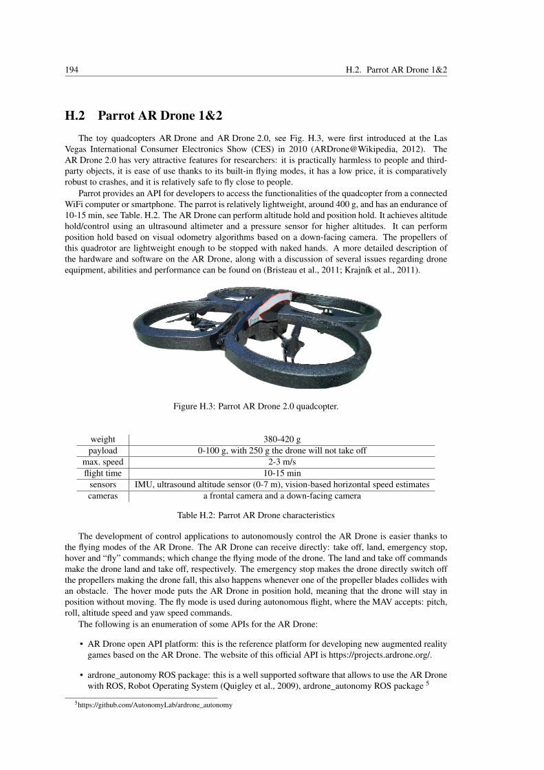
194 H.2. Parrot AR Drone 1&2
H.2 Parrot AR Drone 1&2The toy quadcopters AR Drone and AR Drone 2.0, see Fig. H.3, were first introduced at the Las
Vegas International Consumer Electronics Show (CES) in 2010 (ARDrone@Wikipedia, 2012). TheAR Drone 2.0 has very attractive features for researchers: it is practically harmless to people and third-party objects, it is ease of use thanks to its built-in flying modes, it has a low price, it is comparativelyrobust to crashes, and it is relatively safe to fly close to people.
Parrot provides an API for developers to access the functionalities of the quadcopter from a connectedWiFi computer or smartphone. The parrot is relatively lightweight, around 400 g, and has an endurance of10-15 min, see Table. H.2. The AR Drone can perform altitude hold and position hold. It achieves altitudehold/control using an ultrasound altimeter and a pressure sensor for higher altitudes. It can performposition hold based on visual odometry algorithms based on a down-facing camera. The propellers ofthis quadrotor are lightweight enough to be stopped with naked hands. A more detailed description ofthe hardware and software on the AR Drone, along with a discussion of several issues regarding droneequipment, abilities and performance can be found on (Bristeau et al., 2011; Krajník et al., 2011).
Figure H.3: Parrot AR Drone 2.0 quadcopter.
weight 380-420 gpayload 0-100 g, with 250 g the drone will not take off
max. speed 2-3 m/sflight time 10-15 min
sensors IMU, ultrasound altitude sensor (0-7 m), vision-based horizontal speed estimatescameras a frontal camera and a down-facing camera
Table H.2: Parrot AR Drone characteristics
The development of control applications to autonomously control the AR Drone is easier thanks tothe flying modes of the AR Drone. The AR Drone can receive directly: take off, land, emergency stop,hover and “fly” commands; which change the flying mode of the drone. The land and take off commandsmake the drone land and take off, respectively. The emergency stop makes the drone directly switch offthe propellers making the drone fall, this also happens whenever one of the propeller blades collides withan obstacle. The hover mode puts the AR Drone in position hold, meaning that the drone will stay inposition without moving. The fly mode is used during autonomous flight, where the MAV accepts: pitch,roll, altitude speed and yaw speed commands.
The following is an enumeration of some APIs for the AR Drone:
• AR Drone open API platform: this is the reference platform for developing new augmented realitygames based on the AR Drone. The website of this official API is https://projects.ardrone.org/.
• ardrone_autonomy ROS package: this is a well supported software that allows to use the AR Dronewith ROS, Robot Operating System (Quigley et al., 2009), ardrone_autonomy ROS package 5
5https://github.com/AutonomyLab/ardrone_autonomy

Appendix H. Utilized Multirotor MAV Platforms 195
• CVG Framework for interfacing with MAVs (Mellado Bataller, I., 2012; Mellado-Bataller, Mejias,et al., 2012; Mellado-Bataller, Pestana, et al., 2013): it is an open framework which objective is tosimplify the development of control applications for quadcopters.
This Vertical Take-Off and Landing (VTOL) MAV has proven to be a realiable platform for visionbased navigation algorithm prototyping. These are but just a few of the projects developed by developersand researchers:
• Autonomous flight in hallways and navigation in stairs using computer vision (Bills et al., 2011).
• Indoors navigations and surveillance applications with cooperative ground robots and the ARDrone (Faigl et al., 2010; Krajník et al., 2010).
• Autonomous flight through a forest using visual-based reactive control (Ross et al., 2013).
• Autonomous navigation using the well-known visual SLAM algorithm PTAM (Engel et al., 2012a;Engel et al., 2012b)
• Active exploration of indoor environments Mostegel et al., 2014.

196 H.3. DJI M100 Quadcopter
H.3 DJI M100 Quadcopter
Figure H.4: Fully equipped DJI M100 quadcopter. The equipment includes the DJI Manifold onboardcomputer, the DJI Guidance sensing system and the DJI Zenmuse X3 gimbal camera.
This quadcopter, shown in Fig. H.5, is a developer platform from DJI, which has similar capabilitiesto the Asctec Pelican: attitude and thrust or altitude speed control or GPS-based flight. Therefore themain user for this quadcopter are developers aiming to work in civilian applications for MAVs. The DJIM100 is very well integrated with DJI specific sensors: DJI Zenmuse line gimbal cameras and the DJIGuidance sensor, which has 5 stereo head cameras specifically designed for obstacle detection and visualodometry. The preferred onboard computer for this quadcopter is the DJI Manifold. It has a payloadcapability of 1000 g and a flight time varying in the 10-25min range. DJI offers an API to interface withthe Quadcopter6, and an associated ROS node7.
H.3.1 DJI M100 Multirotor Experimental Setup - DJIC 2016The following lists summarize the specifications and capabilities of the equipment that is available on
our DJI M100 quadcopter MAV. The list only details the main characteristics of the equipment that weconsider important from a technical point of view.
[Fig. H.5] DJI Matrice 100 Quadrotor:• Equipment and payload:
– DJI Manifold Onboard Computer, 197g– DJI Guidance Sensing System, 337g– DJI Zenmuse X3 Gimbal and Camera, 221g– (x1) DJI TB47D Flight Battery, 600g, 4500mah, 6-cell battery (22.2V nominal)
6https://github.com/dji-sdk/Onboard-SDK-ROS7ttps://github.com/dji-sdk/Onboard-SDK

Appendix H. Utilized Multirotor MAV Platforms 197
Figure H.5: Picture of our fully equipped DJI Matrice 100 Quadrotor MAV.
• Fully equipped DJI M100 quadcopter MAV:– Weight: 3.2Kg– Flight-time: ∼10min– Size, propeller tip-to-tip quadrotor diameter: 0.996m
• Autopilot Control Interfaces:– Lowest-level: roll, pitch and yaw_rate attitude commands {φ ,θ , dψ
dt }c, and thrust Tc.– Highest-level: desired velocity {vx,vy,vz} and heading /yaw rotation speeds ωψ .
[Fig. H.6] Onboard Computer - DJI Manifold:• (Very similar to) Nvidia Jetson TK1 development board:• Ubuntu 14.04 and Robot Operating System (ROS) Indigo• Processors:
– Quad-core, 4-Plus-1 ARM Cortex-A15 MPcore Processor with NEON technology– Low-power NVIDIA Kepler-based GeForce graphics processor
• Memory: 2GB DDR3L system RAM
DJI M100 Autopilot Board
GPS Module
NVIDIA Jetson TK1- Quad-core ARM Processor- NVIDIA Kepler GPU
Figure H.6: MAV Hardware - Onboard Computer, Autopilot and GPS Module
[Fig. H.7] DJI Guidance Visual Sensing System:• Embedded computing hardware: DJI Guidance Core - [Very similar to] Altera Cyclone V (low-cost
SoC FPGA) - FPGA + dual Core ARM Processor.• Sensors:
– Built-in IMU

198 H.3. DJI M100 Quadcopter
DJI Guidance SystemGuidance Core(5x) Stereo Camera (5x) Distance Sensor
Figure H.7: MAV Hardware - Guidance Sensing System, which is composed of 5 stereo heads and anembedded processing unit.
Gimbal and CameraDJI Zemuse X3
DJI Guidance SystemGuidance Core(5x) Stereo Camera (5x) Distance Sensor
Figure H.8: MAV Hardware - Gimbal Camera and Guidance Sensing System, which is composed of 5stereo heads and an embedded processing unit.
– (x5) Stereo camera heads: front, rear, left, right and bottom
* Built-in ultrasonic distance sensor
* Built-in stereo camera pair• Velocity measurement (only from downwards looking stereo head), 0-16m/s at 2m altitude• Embedded visual-inertial odometry algorithm from DJI to estimate the motion of the MAV in GPS-
denied/degraded environments. Integrates the IMU measurements with the five camera view direc-tions (monocular or stereo depending on current conditions). The visual-inertial odometry algo-rithm is described in the following three scientific works (Zhou, Fang, et al., 2015; Zhou, Liu, et al.,2014; Zhou, Ye, et al., 2014).
• Acquisition rate of the sensors configured using a GUI from DJI[Fig. H.8] DJI Zenmuse X3 Gimbal and Camera:
• Note: Max. resolution is ∼4K standard, but the resolution available onboard: image frame is 1280X 720 pixel (pixel format NV12)
• Gimbal position commands are directed through the Autopilot, the Gimbal is very well stabilized.
Appendix H. Utilized Multirotor MAV Platforms 199
H.4 Appendix BibliographyAscendingTechnologies (2010). Ascending Technologies. http://www.asctec.de (cit. on p. 192).Bills, C., Chen, J., and Saxena, A. (2011). “Autonomous MAV flight in indoor environments using single
image perspective cues”. In: Robotics and Automation (ICRA), 2011 IEEE International Conferenceon, pp. 5776–5783 (cit. on p. 195).
Bristeau, P.-J., Callou, F., Vissiere, D., Petit, N., et al. (2011). “The navigation and control technologyinside the ar. drone micro uav”. In: 18th IFAC World Congress. Vol. 18, pp. 1477–1484 (cit. on pp. 193,194).
Mellado Bataller, I. (2012). A new framework for interfacing with MAVs. https://github.com/uavster/mavwork (cit. on pp. 192, 193, 195).
Engel, J., Sturm, J., and Cremers, D. (2012a). “Camera-Based Navigation of a Low-Cost Quadrocopter”.In: Proc. of the International Conference on Intelligent Robot Systems (IROS) (cit. on p. 195).
Engel, J., Sturm, J., and Cremers, D. (2012b). “Accurate figure flying with a quadrocopter using onboardvisual and inertial sensing”. IMU 320, p. 240 (cit. on p. 195).
Faigl, J., Krajník, T., Vonásek, V., and Preucil, L. (2010). “Surveillance Planning with Localization Un-certainty for UAVs”. In: 3rd Israeli Conference on Robotics, Ariel: Ariel University Center, pages(cit. on p. 195).
Honegger, D., Meier, L., Tanskanen, P., and Pollefeys, M. (2013). “An open source and open hardwareembedded metric optical flow cmos camera for indoor and outdoor applications”. In: Robotics andAutomation (ICRA), 2013 IEEE International Conference on. IEEE, pp. 1736–1741 (cit. on p. 193).
Krajník, T., Faigl, J., Vonásek, V., Košnar, K., Kulich, M., and Preucil, L. (2010). “Simple, Yet StableBearing-Only Navigation”. Journal of Field Robotics 27.5, pp. 511–533 (cit. on p. 195).
Krajník, T., Vonásek, V., Fišer, D., and Faigl, J. (2011). “AR-Drone as a Platform for Robotic Researchand Education”. In: Research and Education in Robotics: EUROBOT 2011. Heidelberg: Springer (cit.on p. 194).
Mellado-Bataller, I., Mejias, L., Campoy, P., and Olivares-Mendez, M. A. (2012). “Rapid prototypingframework for visual control of autonomous micro aerial vehicles”. In: 12th International Conferenceon Intelligent Autonomous System (IAS-12). Jeju Island, Korea (cit. on p. 195).
Mellado-Bataller, I., Pestana, J., Olivares-Mendez, M. A., Campoy, P., and Mejias, L. (2013). “MAVwork:a framework for unified interfacing between micro aerial vehicles and visual controllers”. In: Frontiersof Intelligent Autonomous Systems. Springer, pp. 165–179 (cit. on p. 195).
Mostegel, C., Wendel, A., and Bischof, H. (2014). “Active monocular localization: Towards autonomousmonocular exploration for multirotor mavs”. In: Robotics and Automation (ICRA), 2014 IEEE Inter-national Conference on. IEEE, pp. 3848–3855 (cit. on p. 195).
Quigley, M., Gerkey, B., Conley, K., Faust, J., Foote, T., Leibs, J., Berger, E., Wheeler, R., and Ng,A. (2009). “ROS : an open-source Robot Operating System”. In: IEEE International Conference onRobotics and Automation (ICRA 2009) (cit. on p. 194).
Achtelik, Markus (2011). ROS asctec_mav_framework repository, https://github.com/ethz-asl/asctec_mav_framework (cit. on p. 192).
Ross, S., Melik-Barkhudarov, N., Shankar, K. S., Wendel, A., Dey, D., Bagnell, J. A., and Hebert, M.(2013). “Learning monocular reactive uav control in cluttered natural environments”. In: Robotics andAutomation (ICRA), 2013 IEEE International Conference on. IEEE, pp. 1765–1772 (cit. on p. 195).
Sanchez-Lopez, J. L., Fernández, R. A. S., Bavle, H., Sampedro, C., Molina, M., Pestana, J., and Campoy,P. (2016). “Aerostack: An architecture and open-source software framework for aerial robotics”. In:Unmanned Aircraft Systems (ICUAS), 2016 International Conference on. IEEE, pp. 332–341 (cit. onp. 193).
UAS Technologies Sweden AB Company (2012). UAS Technologies Sweden AB Company website.http://www.uastech.com/ (cit. on p. 191).
CVG-UPM (2012). Universidad Politécnica de Madrid. Computer Vision Group. Vision for UAV Project.http://www.vision4uav.com (cit. on p. 192).
ARDrone@Wikipedia (2012). Parrot AR Drone article at english Wikipedia. http : / / en .wikipedia.org/wiki/Parrot_AR.Drone (cit. on p. 194).
Zhou, G., Fang, L., Tang, K., Zhang, H., Wang, K., and Yang, K. (2015). “Guidance: A Visual SensingPlatform For Robotic Applications”. In: Proceedings of the IEEE Conference on Computer Vision andPattern Recognition Workshops, pp. 9–14 (cit. on p. 198).

200 H.4. Appendix Bibliography
Zhou, G., Liu, A., Yang, K., Wang, T., and Li, Z. (2014). “An embedded solution to visual mapping forconsumer drones”. In: Proceedings of the IEEE Conference on Computer Vision and Pattern Recog-nition Workshops, pp. 656–661 (cit. on p. 198).
Zhou, G., Ye, J., Ren, W., Wang, T., and Li, Z. (2014). “On-board inertial-assisted visual odometer onan embedded system”. In: 2014 IEEE International Conference on Robotics and Automation (ICRA).IEEE, pp. 2602–2608 (cit. on p. 198).
Appendix IInternational Micro Aerial VehicleCompetitions
This appendix provides a short description and a summary of the achieved results for each of the aerialrobotics competitions in which, to this date, some of the algorithms developed during this thesis has beenused. The description will be kept concise, but the link to the main website of the competition and tothe competition rules, when available, are provided. The following are the competitions and the eventsin which the author of the thesis either participated directly and/or tutored students and/or some of thealgorithms presented in this thesis were utilized by his colleagues.
• 2016 DJI Developer Challenge - DJIC 2016
• International Micro Air Vehicle Conference and Flight Competition 2016 - IMAV 2016
• European Robotics Challenges 2014 - Simulation Challenge 3 - EuRoC 2014
• International Aerial Robotics Competition 2014 - Mission 7 - IARC 2014
• International Micro Air Vehicle Conference and Flight Competition 2013 - IMAV 2013
• International Micro Air Vehicle Conference and Flight Competition 2012 - IMAV 2012
• Concurso en Ingeniería de Control 2012 - CEA 2012
201
202 I.1. 2016 DJI Developer Challenge - DJIC 2016
I.1 2016 DJI Developer Challenge - DJIC 2016
I.1.1 External Links• Website: https://developer.dji.com/challenge2016/• Rules: https://dl.djicdn.com/downloads/dev/DevChallenge2016/2016%20DJI%20Developer%20Challenge%20Official%20Rules_v1.0.pdf
• Teams qualified for final round:https://developer.dji.com/news/2016-dji-developer-challenge-10-teams-enter-final-round/
• DJI’s summary video: https://youtu.be/DIRkzH3cTAM
I.1.2 Short descriptionThis competition was organized by DJI, a manufacturer of UAVs, mainly multicopters, and related
products such as flight controllers and propulsion systems; gimbal stabilized mounts for cameras andcameras. The competition proposed an outdoor emulated search and rescue scenario. The participantshad to submit a proposal and get selected to participate, and later on get qualified in successive stagesof the competition in order to be able to participate in the finals. The hardware for the competition wasmostly supplied by DJI, with little space to use alternatives, and included: the DJI M100 quadcopter, theDJI Guidance sensing system, the DJI Zenmuse X3 Gimbal and the DJI Manifold onboard computer.
The competition hosted only one event, in which a team from the TU Graz participated and qualifiedto participate in the finals. It featured an emulated search and rescue mission, whose main objectives were:(0) perform the mission completely in Autonomous mode with no interaction with the pilot, (1) take-offfrom a moving vehicle, (2) enter a search area and find survivors, emulated using small fiducial markers,and (3) come back to the pick-up area and land on a moving vehicle, alternatively on a static vehicle.
I.1.3 Achieved ResultsExperimental MAV Platform: DJI M100 as described in Sec. H.3.1.
Contributions of author to results:• Module utilized in autonomous flight architecture: trajectory and speed planner presented in Ch. 4.• Other roles of the author as part of the team: team leader, main system integrator, experimental
tester and being part of the team members participating and performing the MAV deployment inthe event finals.
Achieved Results:The competition recreated a drone Search and Rescue scenario. The “Graz Griffins” team qualifiedthrough successive rounds, from the initial ≈140 teams, to be part of the last 10 teams showing theirsolution experimentally in the finals.
At the time of the competition our MAV could perform the following tasks autonomously:• take-off from a moving vehicle,• produce a map performing an overview flight of an area using only onboard computation,• use the created map to navigate safely avoiding obstacles while adding new obstacles to the map,• land on the static vehicle.We were not able to integrate all these tasks in a single flight for the competition. However, overall our
team showed a very innovative solution using on-board mapping based on photogrammetry algorithms1.The on-board calculated map is converted to an obstacle-map that can be used by the presented plannerto deliver trajectories that are then executed by the controller, all in the same flight and without requiringany off-board computation.
1DJIC 2016 video playlist: http://bit.ly/2faublQ
Appendix I. International Micro Aerial Vehicle Competitions 203
I.2 International Micro Air Vehicle Conference and FlightCompetition 2016 - IMAV 2016
I.2.1 External Links• Website: http://www.imavs.org/2016/• Rules: http://www.imavs.org/2016/documents/IMAV2016_Competition_rules_v2.3.pdf• Results: http://www.imavs.org/2016/result.html• Proceedings: http://www.imavs.org/imav2016proceedings/• Video of proposal: https://vimeo.com/156657670
I.2.2 Short descriptionThis competition proposed two events, an outdoor mission and an indoor mission. The choice of
MAV, sensors and autonomy level are quite open; but the scoring system promotes autonomy, althoughmanual piloting entries are also accepted, and very heavily custom lightweight MAVs. Therefore, thiscompetitions tries to attract and bring both: robotics autonomy and new lightweight MAV designs.
The main objectives of the IMAV 2016 Indoor Competition, in which the CVG_UPM participated,were: (1) take-off, (2) enter a building, several options are available, (3) pick up and release items, (4) exitthe building, (5) land, with also several options are available and (6) build a map of the environment.
I.2.3 Achieved Results - Indoor CompetitionExperimental MAV Platform: custom MAV based on the Pixhawk Autopilot2.
Contributions of author to results:• Module utilized in autonomous flight architecture: controller presented in Ch. 2.
Achieved Results:At the time of the competition our MAV could perform the following tasks autonomously:
• take-off,• enter a building through the door,• pick up and release items,• exit the building,• land.The CVG_UPM team was able to solve multiple tasks in fully autonomous mode and was the team to
achieve the highest number of tasks, although in separate flights, in fully autonomous mode3. Despite itsoutstanding performance, the CVG team earned the 4th position due to the scoring system leaning veryheavily towards the usage of very small MAVs.
2https://pixhawk.org/3IMAV 2016 video playlist: https://goo.gl/tdZyGu

204 I.3. European Robotics Challenges 2014 - Simulation Challenge 3 - EuRoC 2014
I.3 European Robotics Challenges 2014 - Simulation Challenge 3 -EuRoC 2014
I.3.1 External Links• Website: http://www.euroc-project.eu/index.php?id=euroc_project• Challenge 3: http://www.euroc-project.eu/index.php?id=challenge_3• Rules: http://www.euroc-project.eu/index.php?id=motivation0• Results (Simulation Challenge 3):http://www.euroc-project.eu/index.php?id=simulation_challenge3
• Publications: http://www.euroc-project.eu/index.php?id=publications
I.3.2 Short descriptionThe European Robotics Challenges (EuRoC) have a very general motivation, they seek to accelerate
the adoption of robotics by the industry. The first challenge started in 2014, and included three main eventcategories:
Challenge 1 - Reconfigurable Interactive Manufacturing Cell - research in advanced concepts forrobotic arm manipulators.
Challenge 2 - Shop Floor Logistics and Manipulation - robotic object manipulation from mobilerobots equipped with an arm manipulator.
Challenge 3 - Plant Servicing and Inspection - integration of MAVs in industrial environments.
The first stage of all three challenges was a simulation competition with precise scoring rules, eval-uated using an automatic script. The 10 top qualified teams passed to the next stage, which promotedthe proposal along with an industry partner of innovative high impact projects. The TU Graz participatedin Challenge 3. The simulation challenge of this track required the development of algorithms for threeseparate tasks. These three tasks were scored separately and had the following objectives, which applyvery well to MAVs:
• The development of high precision real-time vision-based localization algorithms.
• The development of high precision real-time obstacle mapping algorithms.
• The development of state-estimation, trajectory control and trajectory planning algorithms.
I.3.3 Achieved Results - EuRoC 2014 - Challenge 3 - Simulation CompetitionExperimental MAV Platform: simulated MAV, prepared by competition organizers.
Contributions of author to results:• Module utilized in autonomous flight architecture: trajectory and speed planner presented in Ch. 4.• Other roles of the author as part of the team: close collaboration with main developer of the state
estimator and controller used in the flight simulation.
Achieved Results:The developed fast real-time trajectory and speed planner4 enabled reliable obstacle avoidance and veryfast trajectory execution by the simulated quadrotor that replicated the capabilities of an Asctec Firefly.
The “Graz Griffins” team achieved the 6th position out of 21 teams, which included world renownedEuropean universities and laboratories, in the EuRoC 2014 - Challenge 3 - Simulation Competition. Thisfact enabled the team to present a proposal in collaboration with a company to the next stage of EuRoC.
4EuRoC 2014 trajectory flight video: http://bit.ly/2cQnO6I

Appendix I. International Micro Aerial Vehicle Competitions 205
I.4 International Aerial Robotics Competition 2014 - Mission 7 -IARC 2014
I.4.1 External Links• Website: http://www.aerialroboticscompetition.org/index.php• Rules - Mission 7: http://www.aerialroboticscompetition.org/rules.php• Proceedings: http://www.aerialroboticscompetition.org/symposium2014.php• Competitors: http://www.aerialroboticscompetition.org/competitors.php
I.4.2 Short descriptionThe International Aerial Robotics Competition (IARC) seeks to propose high difficulty robotic chal-
lenges that are currently not solved by either universities or industry. The organization proposes a“Mission” which is yearly organized as a competition event with little changes in the rules until a par-ticipant is able to achieve the proposed objectives. Once a team is able to demonstrate a solution to thecurrent objectives, a new “Mission” is conceived. After three decades of IARC challenges, the current“Mission” is Mission 7. Past challenges, Mission 5 and Mission 6, have already tackled MAV indoorsnavigation, autonomous exploration, Simultaneous Localization and Mapping (SLAM) and small objectsearch, picking and delivery.
The current objectives proposed in Mission 7, in which the CVG_UPM participated in 2014, areextremely challenging and require the combination of: MAV odometry localization, object detection, rea-soning on the behavior of a of group ground robots, autonomous decision making by the MAV and in thefuture also to reason on the behavior of another challenger MAV. More precisely, the flight environment isa square region where 2 sets of ground robots are navigating autonomously, 1 set are the target robots andthe others are obstacles, which hold columns. The MAV has to navigate in this area avoiding obstacles andcan affect the navigation direction of the target robots by interacting physically with them, which follow apseudo-random navigation behavior. The main objective of the challenge is for the MAV to successfullyredirect 4 or more target robots to exit the challenge square area through one specific border.
I.4.3 Achieved Results - IARC 2014 - Asia VenueExperimental MAV Platform: Asctec Pelican as described in Sec. H.1.2.
Contributions of author to results:• Modules utilized in autonomous flight architecture: controller presented in Ch. 2 and state estimator
presented in Appx. E.• Other roles of the author as part of the team: system integrator, experimental tester and being part
of the team members participating and performing the MAV deployment in the competition event.
Achieved Results:At the time of the competition our MAV could perform the following tasks autonomously:
• take-off,• navigate inside the competition area,• ground-robot detection,• simple ground robot avoidance technique,• land.Same as other teams, we were still far from achieving the interaction with the ground robots. There-
fore, the CVG_UPM5 team showed similar capabilities to other contestants. Our level of developmentwas good as a first step towards continuing our participation the next year for IARC 2015.
5IARC 2014 video playlist: https://goo.gl/bEvK3F

206 I.5. International Micro Air Vehicle Conference and Flight Competition 2013 - IMAV 2013
I.5 International Micro Air Vehicle Conference and FlightCompetition 2013 - IMAV 2013
I.5.1 External Links• Website: http://www.imavs.org/2013/index.html• Rules 1: http://www.imavs.org/2013/index.php/information.html• Rules 2: http://www.imav2013.org/images/IMAV2013_General_Rules.pdf• Results 1: http://www.imavs.org/imav2013/• Results 2: http://www.imavs.org/2013/index.php/final-results.html• Proceedings: http://www.imavs.org/imav2013proceedings/
I.5.2 Short descriptionThis competition proposed two events, an outdoor mission and an indoor mission. The choice of
MAV, sensors and autonomy level are quite open; but the scoring system promotes autonomy, althoughmanual piloting entries are also accepted, and very heavily custom lightweight MAVs. Therefore, thiscompetitions tries to attract and bring both: robotics autonomy and new lightweight MAV designs.
The main objectives of the IMAV 2013 Indoor Mission, in which the CVG_UPM participated, were:(1) take-off, (2) cross a window, with two available options, (3) several navigation objectives through andaround an area with column obstacles, (4) column obstacle detection and (5) alternative tasks such asmoving landing, static landing and precise object dropping.
I.5.3 Achieved Results - Indoor MissionExperimental MAV Platform: multi-robot solution using the AR Drone 2.0, see Appx. H.2.
Contributions of author to results:• Modules utilized in autonomous flight architecture: controller presented in Ch. 2 and state estimator
presented in Appx. E, integrated as part of a ROS-based multi-robot autonomous system.• Other roles of the author as part of the team: system integrator, experimental tester and being part
of the team members participating and performing the MAV deployment in the competition event.
Achieved Results:At the time of the competition our MAV could perform the following tasks autonomously:
• take-off,• localization achieved by placing visual fiducial markers in the competition arena,• enter the navigation area by crossing the big window,• multi-robot navigation around the obstacle area,• multi-robot navigation through unknown obstacle area,• land on static target.The CVG_UPM showed an outstanding multi-robot autonomous solution to IMAV 20136. The team
that represented the UPM and the Computer Vision Group (CVG, UPM) was awarded with: first place in“Indoor Autonomy - IMAV 2013”.
6IMAV 2013 video playlist: https://goo.gl/KosWKH

Appendix I. International Micro Aerial Vehicle Competitions 207
I.6 International Micro Air Vehicle Conference and FlightCompetition 2012 - IMAV 2012
I.6.1 External Links• Website: http://www.imavs.org/2012/• Rules: http://hadmernok.hu/132_31_bekesib.pdf• Results: http://www.imavs.org/imav2012results/• Proceedings: http://www.imavs.org/imav2012proceedings/• Video - AKAFlieg Summary: https://www.youtube.com/watch?v=E2fwMWeuqGw
I.6.2 Short descriptionThis competition proposed two events, an outdoor mission and an indoor mission. The choice of
MAV, sensors and autonomy level are quite open; but the scoring system promotes autonomy, althoughmanual piloting entries are also accepted, and very heavily custom lightweight MAVs. Therefore, thiscompetitions tries to attract and bring both: robotics autonomy and new lightweight MAV designs.
The CVG_UPM participated in the IMAV 2012 Indoor Dynamics Competition. This challenge soughtonly fast navigation and obstacle avoidance objectives. The flight environment had two opposing horizon-tal tubes, each supported by two vertical columns on the sides, and was precisely described in the rules.The main objectives to be achieved were: (1) to perform the localization task in this environment and(2) to perform as many 8-shaped laps around the 2 horizontal tubes as possible.
I.6.3 Achieved Results - Indoor Dynamics CompetitionExperimental MAV Platform: Asctec Pelican, equipped as described in Sec. H.1.1.
Contributions of author to results:• Modules utilized in autonomous flight architecture: controller presented in Ch. 2, state estimator
and particle filter presented in Appx. E.• Other roles of the author as part of the team: system integrator, experimental tester and being part
of the team members participating and performing the MAV deployment in the competition event.
Achieved Results:At the time of the competition our MAV could perform the following tasks autonomously:
• take-off,• localization achieved by a using a Lidar sensor combined with a particle filter,• otherwise, odometry-based state estimation combining different sensor technologies,• perform 8-shaped laps around the 2 horizontal tubes,• land.
The CVG_UPM was the only team to show a fully autonomous solution to the IMAV 2012 Indoor Dy-namics Competition 7. The team that represented the UPM and the Computer Vision Group (CVG) wastwice awarded with:
• the special award “Best Automatic Performance - IMAV 2012”, as part of the overall results of thecompetitions, and
• second place in the “Indoor Flight Dynamics - Rotary Wing MAV” challenge, where the first placewas obtained by a remotely piloted multirotor.
7IMAV 2012 video playlist: https://goo.gl/PRns2D

208 I.7. Contest on Control Engineering 2012 - CEA 2012
I.7 Contest on Control Engineering 2012 - CEA 2012
I.7.1 External Links• Website:http://intranet.ceautomatica.es/og/ingenieria-de-control/benchmark-2011-2012
• Rules: http://intranet.ceautomatica.es/sites/default/files/upload/13/files/Concurso%20IC2012%20-%20Bases(1).pdf
• Video Summary: https://www.youtube.com/watch?v=uWYatwnze-A
I.7.2 Short descriptionThe Contest on Control Engineering 2012 (in Spanish “Concurso en Ingeniería de Control 2012”),
organized by the Spanish Committee of Automation, has the objective of proposing a challenge that canbe solved by bachelor and master students, mainly from the field of control and automation.
By using the off-the-shelf AR Drone MAV, the students could focus on the identification, state-estimation and control tasks. This MAV was probably chosen because it provides out-of-the-box velocityand attitude estimates as part of its telemetry.
The challenge was divided in two stages: simulation and flight competition. For the simulationstage, the scoring was divided in the three main target tasks: (1) model design and identification, and(2) state-estimation and trajectory control. The scoring system in the finals evaluated the tracking errorand the trajectory round-trip time. The CVG_UPM participated with 2 teams, a team of PhD students anda team of undergraduate students, tutored by the PhD students’ team.
I.7.3 Achieved ResultsExperimental MAV Platform: AR Drone 2.0 quadrotor, see Appx. H.2.
Contributions of author to results:• Module utilized in autonomous flight architecture: controller similar to presented in Ch. 2.• Other roles of the author as part of the team: tutoring the undergraduate students’ team and being
part of the team members participating and performing the MAV deployment in the competitionevent.
Achieved Results:Two teams participated representing the Universidad Politécnica de Madrid (UPM) and the ComputerVision Group (CVG_UPM), and were awarded with:
• Undergraduate students’ team of the ETSII-UPM engineering school using their own developedsoftware supervised by J. Pestana: the first (phase 1 - simulation) and third places (final phase -autonomous flight event)
• CVG_UPM PhD students’ team: the second (phase 1 - simulation) and fifth places (final phase -autonomous flight event). In the final phase of the competition our team achieved the fifth place,due to our controller, when compared to other teams, leaning towards low tracking error with higherround-trip times.
Appendix JOther Micro Aerial VehicleAutonomous Flight Demonstrations
The modules developed during the course of this PhD thesis have been used as part of robotics soft-ware architectures to achieve autonomous flight and task execution in several experimental autonomousflight demonstrations. Setting aside their usage as part of the participation in International MAV Compe-titions, which has been described in Appx. I, the presented modules have been utilized in the followingautonomous flight demonstrations.
209

210 J.1. Using Trajectory Controller and/or State Estimator
J.1 Using Trajectory Controller and/or State EstimatorThe controller presented in Chap. 2 and/or the state estimator presented in Appx. E have been show-
cased in the following live demos by the Computer Vision Group of the Universidad Politécnica de Madrid(CVG, UPM):
• CivilDRON 2017 congress1, Madrid (Spain)Simplified version of IMAV 2016 competition missionJanuary 2017
• CivilDRON 2016 congress2, Madrid (Spain)Multi-robot mission and vision-based person followingMay 2016
• Semana de la Ciencia 2015 - Science Week 201534, Madrid (Spain)Multi-robot mission and vision-based person followingNovember 2-15, 2015
• Noche Europea de los investigadores - European Researchers’ Night 20155
Multi-robot mission, vision-based person following and a simple search and rescue mission, whichincluded the usage of a multi-modal human-machine interface with the MAV.Madrid (Spain), September 2015
• Semana de la Ciencia 2014 - Science Week 20146, Madrid (Spain)Multi-robot mission and vision-based person followingNovember 2014
• Semana de la Ciencia 2013 - Science Week 20137, Madrid (Spain)Multi-robot mission and vision-based person followingNovember 4-17, 2013
1CivilDRON 2017: http://www.civildron.com/2CivilDRON 2016: http://www.aerpas.es/wp-content/uploads/2015/04/CivilDRON16_v2.pdf3Semana de la Ciencia 2015 - Website:http://bit.ly/2lN9RNg4Semana de la Ciencia 2015 - Results Report:http://bit.ly/2muELHG5European Researchers’ Night 2015 - Website: http://bit.ly/2mM6a9Q6Semana de la Ciencia 2014 - Results Report:http://bit.ly/2lNg1NA7Semana de la Ciencia 2013 - Results Report:http://bit.ly/2npz2lF

Appendix J. Other Micro Aerial Vehicle Autonomous Flight Demonstrations 211
J.2 Using Visual Servoing ArchitectureThe aerial robotics visual servoing architecture presented in Chap. 3 has been showcased in the fol-
lowing live demos mostly by the CVG (UPM), and one demo by the Institute of Computer Graphics of theGraz University of Technology (ICG, TU Graz). These demonstrations have shown the MAV performinga person following task:
• CivilDRON 2016 congress8, Madrid (Spain)Multi-robot mission and vision-based person followingMay 2016
• Semana de la Ciencia 2015 - Science Week 2015910, Madrid (Spain)Multi-robot mission and vision-based person followingNovember 2-15, 2015
• 2015 European Robotics Week1112, Madrid (Spain)Vision-based person followingSeptember 2015
• Noche Europea de los investigadores - European Researchers’ Night 201513
Multi-robot mission, vision-based person following and a simple search and rescue missionMadrid (Spain), September 2015
• 2014 European Robotics1415, Madrid (Spain)Vision-based person followingNovember 2014
• Semana de la Ciencia 2014 - Science Week 201416, Madrid (Spain)Multi-robot mission and vision-based person followingNovember 2014
• OpenLabNight 201417, ICG - TU Graz (Austria)Vision-based person followingOctober 9, 2014
• Semana de la Ciencia 2013 - Science Week 201318, Madrid (Spain)Multi-robot mission and vision-based person followingNovember 4-17, 2013
• The 11th IEEE International Symposium on Safety, Security, and Rescue Robotics (SSRR 2013)19
Vision-based person followingLinköping (Sweden), October 21-26, 2013
8CivilDRON 2016: http://www.aerpas.es/wp-content/uploads/2015/04/CivilDRON16_v2.pdf9Semana de la Ciencia 2015 - Website:http://bit.ly/2lN9RNg
10Semana de la Ciencia 2015 - Results Report:http://bit.ly/2muELHG112015 European Robotics Week - Website: http://bit.ly/2mcMglt12European Robotics Week - Website: http://bit.ly/2mT12Bh13European Researchers’ Night 2015 - Website: http://bit.ly/2mM6a9Q142014 European Robotics Week - Website: http://bit.ly/2mMaTIV15European Robotics Week - Website: http://bit.ly/2mT12Bh16Semana de la Ciencia 2014 - Results Report:http://bit.ly/2lNg1NA17OpenLabNight 2014, ICG - TU Graz, Website: http://bit.ly/2mwigU418Semana de la Ciencia 2013 - Results Report:http://bit.ly/2npz2lF19SSRR 2013 Demos Website:http://www.ssrr-conference.org/2013/Demos.html

212 J.3. Using Trajectory and Speed Planner
J.3 Using Trajectory and Speed PlannerThe works related to the 2016 DJI Developer Challenge, which entailed the improvement and
development of the trajectory planner presented in Chap. 4, have been showcased, representing theICG - TU Graz, in the following two public events:
• An experimental fully autonomous package delivery flight demonstration made by theICG - TU Graz20in collaboration with the company SFL Technologies as part of the roll-out of theirbrand new electric vehicle, the ELI. The roll-out of this vehicle and the autonomous flight demohave been described by two Austrian newspapers: Mein Bezirk21 and Kleine Zeitung22.November 2016
• A public presentation, with no experimental flights, named Intelligent Search and Rescue Dronein the world renowned Ars Electronica Festival 2016 - DroneLab - FutureLab23. This festivalshows modern artwork that utilizes technology as a medium of expression and tries to deliver anoutstanding and open view of current technology developments to its public.September 8-12, 2016
20Fully autonomous package delivery flight demonstration: https://youtu.be/bxM6dls2wuo21ELI roll-out - Mein Bezirk - http://bit.ly/2hott8t22ELI roll-out - Kleine Zeitung - http://bit.ly/2it6N2P23Ars Electronica Festival 2016 - DroneLab: http://www.aec.at/radicalatoms/en/ars-electronica-dronelab/
Bibliography
Abdul Shukor, S. (2013). “A geometrical-based approach to recognise structure of complex interiors”.PhD thesis. University of Warwick.
Abeywardena, D., Kodagoda, S., Dissanayake, G., and Munasinghe, R. (2013). “Improved State Esti-mation in Quadrotor MAVs: A Novel Drift-Free Velocity Estimator”. IEEE Robotics & AutomationMagazine 20.4, pp. 32–39.
Achtelik, M., Achtelik, M., Weiss, S., and Siegwart, R. (2011). “Onboard IMU and monocular visionbased control for MAVs in unknown in- and outdoor environments”. In: Robotics and Automation(ICRA), 2011 IEEE International Conference on, pp. 3056–3063.
Achtelik, M. W., Lynen, S., Chli, M., and Siegwart, R. (2013). “Inversion based direct position controland trajectory following for micro aerial vehicles”. In: Intelligent Robots and Systems (IROS), 2013IEEE/RSJ International Conference on. IEEE, pp. 2933–2939.
Achtelik, M. W., Lynen, S., Weiss, S., Kneip, L., Chli, M., and Siegwart, R. (2012). “Visual-inertial SLAMfor a small helicopter in large outdoor environments”. In: Intelligent Robots and Systems (IROS), 2012IEEE/RSJ International Conference on. IEEE, pp. 2651–2652.
Achtelik, M., Bachrach, A., He, R., Prentice, S., and Roy, N. (2009). “Stereo vision and laser odometryfor autonomous helicopters in GPS-denied indoor environments”. In: SPIE Defense, Security, andSensing. International Society for Optics and Photonics, pp. 733219–733219.
Aerosystems, B. (1999). “Civilian applications: the challenges facing the UAV industry”. Air & SpaceEurope.
Agrachev, A. A. and Sachkov, Y. (2004). Control theory from the geometric viewpoint. Vol. 2. SpringerScience & Business Media.
Mani Monajjemi (2012). ardrone_autonomy : A ROS Driver for ARDrone 1.0 & 2.0. https : / /github.com/AutonomyLab/ardrone_autonomy. Autonomy Lab, Simon Fraser Univer-sity.
Argyros, A., Georgiadis, P., Trahanias, P., and Tsakiris, D. (2002). “Semi-autonomous Navigation of aRobotic Wheelchair”. Journal of Intelligent and Robotic Systems 34 (3), pp. 315–329.
Ars Electronica Linz Gmbh (2012). SPAXELS: DRONE SHOWS SINCE 2012. https : / / www .spaxels.at/. Accessed: 2017-03-19.
Arulampalam, M. S., Maskell, S., Gordon, N., and Clapp, T. (2002). “A tutorial on particle filters foronline nonlinear/non-Gaussian Bayesian tracking”. Signal Processing, IEEE Transactions on 50.2,pp. 174–188.
AscendingTechnologies (2010). Ascending Technologies. http://www.asctec.de.Babenko, B., Yang, M.-H., and Belongie, S. (2009). “Visual tracking with online Multiple Instance Learn-
ing”. In: Computer Vision and Pattern Recognition, 2009. CVPR 2009. IEEE Conference on, pp. 983–990.
213
214 Bibliography
Bachrach, A. G. (2009). “Autonomous flight in unstructured and unknown indoor environments”. MAthesis. Massachusetts Institute of Technology.
Bachrach, A., Prentice, S., He, R., and Roy, N. (2011). “RANGE-Robust autonomous navigation in GPS-denied environments”. Journal of Field Robotics 28.5, pp. 644–666.
Baker, S. and Matthews, I. (2004). “Lucas-kanade 20 years on: A unifying framework”. Internationaljournal of computer vision 56.3, pp. 221–255.
Barfoot, T., Forbes, J. R., and Furgale, P. T. (2011). “Pose estimation using linearized rotations and quater-nion algebra”. Acta Astronautica 68.1, pp. 101–112.
Bento, M. (2008). “Unmanned aerial vehicles: an overview”. Inside GNSS 3.1, pp. 54–61.Bills, C., Chen, J., and Saxena, A. (2011). “Autonomous MAV flight in indoor environments using single
image perspective cues”. In: Robotics and Automation (ICRA), 2011 IEEE International Conferenceon, pp. 5776–5783.
Blyenburgh, P. v. (2006). “UAV Systems : Global Review”. In: Avionics’06 Conference. Amsterdam, TheNetherlands.
Bouabdallah, Samir, Murrieri, Pierpaolo, and Siegwart, Roland (2005). “Towards Autonomous IndoorMicro VTOL”. Autonomous Robots 18 (2). 10.1007/s10514-005-0724-z, pp. 171–183.
Bouabdallah, Samir and Siegwart, Roland (2007). “Full control of a quadrotor”. In: Intelligent robots andsystems, 2007. IROS 2007. IEEE/RSJ international conference on. IEEE, pp. 153–158.
Bouabdallah, S., Murrieri, P., and Siegwart, R. (2005). “Towards autonomous indoor micro VTOL”. Au-tonomous Robots 18.2, pp. 171–183.
Bouabdallah, S. and Siegwart, R. (2005). “Backstepping and sliding-mode techniques applied to an indoormicro quadrotor”. In: Robotics and Automation, 2005. ICRA 2005. Proceedings of the 2005 IEEEInternational Conference on. IEEE, pp. 2247–2252.
Bourquardez, O., Mahony, R., Guenard, N., Chaumette, F., Hamel, T., and Eck, L. (2009). “Image-BasedVisual Servo Control of the Translation Kinematics of a Quadrotor Aerial Vehicle”. Robotics, IEEETransactions on 25.3, pp. 743–749.
Breckenridge, W. (1999). “Quaternions proposed standard conventions”. Jet Propulsion Laboratory,Pasadena, CA, Interoffice Memorandum IOM, pp. 343–79.
Bristeau, P.-J., Callou, F., Vissiere, D., Petit, N., et al. (2011). “The navigation and control technologyinside the ar. drone micro uav”. In: 18th IFAC World Congress. Vol. 18, pp. 1477–1484.
Burschka, D. and Mair, E. (2008). “Direct pose estimation with a monocular camera”. In: Robot Vision.Springer, pp. 440–453.
Campoy, P., Correa, J. F., Mondragón, I., Martínez, C., Olivares, M., Mejías, L., and Artieda, J. (2009).“Computer Vision Onboard UAVs for Civilian Tasks”. Journal of Intelligent and Robotic Systems54.1-3, pp. 105–135.
Castillo, P., Dzul, A., and Lozano, R. (2004). “Real-time stabilization and tracking of a four-rotor minirotorcraft”. Control Systems Technology, IEEE Transactions on 12.4, pp. 510–516.
Castillo, P., Lozano, R., and Dzul, A. (2005). “Stabilization of a mini rotorcraft with four rotors”. IEEEControl Systems Magazine 25.6, pp. 45–55.
Chaumette, F. (1998). “Potential problems of stability and convergence in image-based and position-basedvisual servoing”. In: The confluence of vision and control. Springer, pp. 66–78.
Cheng, Y. and Crassidis, J. L. (2004). “Particle filtering for sequential spacecraft attitude estimation”. In:Proc. of the 2004 AIAA Guidance, Navigation, and Control Conference, p. 5337.
Chesi, G. (2009). “Visual servoing path planning via homogeneous forms and LMI optimizations”.Robotics, IEEE Transactions on 25.2, pp. 281–291.
Chesi, G. and Vicino, A. (2004). “Visual servoing for large camera displacements”. Robotics, IEEE Trans-actions on 20.4, pp. 724–735.
Comport, A., Mahony, R., and Spindler, F. (2011). “A visual servoing model for generalised cameras: Casestudy of non-overlapping cameras”. In: Robotics and Automation (ICRA), 2011 IEEE InternationalConference on, pp. 5683–5688.
Corke, P. (2011). Robotics, vision and control: fundamental algorithms in MATLAB. Vol. 73. Springer.Corke, P. I. et al. (1996). Visual Control of Robots: high-performance visual servoing. Research Studies
Press Taunton, UK.Cowling, I. D., Yakimenko, O. A., Whidborne, J. F., and Cooke, A. K. (2010). “Direct method based
control system for an autonomous quadrotor”. Journal of Intelligent & Robotic Systems 60.2, pp. 285–316.

Bibliography 215
Crassidis, J. L. (2006). “Sigma-point Kalman filtering for integrated GPS and inertial navigation”.Aerospace and Electronic Systems, IEEE Transactions on 42.2, pp. 750–756.
Crassidis, J. L., Markley, F. L., and Cheng, Y. (2007). “Survey of nonlinear attitude estimation methods”.Journal of Guidance, Control, and Dynamics 30.1, pp. 12–28.
Mellado Bataller, I. (2012). A new framework for interfacing with MAVs. https://github.com/uavster/mavwork.
Danelljan, M., Khan, F. S., Felsberg, M., Granström, K., Heintz, F., Rudol, P., Wzorek, M., Kvarnström,J., and Doherty, P. (2014). “A low-level active vision framework for collaborative unmanned aircraftsystems”. In: Workshop at the European Conference on Computer Vision. Springer, pp. 223–237.
Danelljan, M., Shahbaz Khan, F., Felsberg, M., and Van de Weijer, J. (2014). “Adaptive color attributes forreal-time visual tracking”. In: Proceedings of the IEEE Conference on Computer Vision and PatternRecognition, pp. 1090–1097.
Davison, A. J., Reid, I. D., Molton, N. D., and Stasse, O. (2007). “MonoSLAM: Real-time single cameraSLAM”. IEEE transactions on pattern analysis and machine intelligence 29.6.
Davison, A. J. (1998). “Mobile Robot Navigation Using Active Vision”. PhD thesis. University of Oxford.Davison, R. A. N. and J., A. (2010). “Live Dense Reconstruction with a Single Moving Camera”. In:
Computer Vision and Pattern Recognition.Deng, H., Zhao, X., and How, Z. (2009). “A Vision-Based Ground Target Tracking System for a Small-
Scale Autonomous Helicopter”. Image and Graphics, International Conference on, pp. 739–743.Dijkstra, E. W. (1959). “A note on two problems in connexion with graphs”. Numerische mathematik 1.1,
pp. 269–271.DJI - Da-Jiang Innovations Science and Technology Co., Ltd (2015). DJI Matrice developer drone line.
https://www.dji.com/matrice100. Accessed: 2017-03-18.Doucet, A., De Freitas, N., and Gordon, N. (2001). An introduction to sequential Monte Carlo methods.
Springer.Driessen, B. J. and Robin, A. L. (2004). “A globally convergent tracking controller for the X4 flyer rotor
craft for reference trajectories with positive thrust”. Robotica 22.04, pp. 375–388.Dunbar, N. and Franz, R. (2003). “Online control customization via optimization, based control”.
Software-Enabled Control: Information Technology for Dynamical Systems, p. 149.Engel, Jakob, Sturm, Jürgen, and Cremers, Daniel (2014). “Scale-aware navigation of a low-cost quadro-
copter with a monocular camera”. Robotics and Autonomous Systems 62.11, pp. 1646–1656.Engel, J., Sturm, J., and Cremers, D. (2012a). “Camera-Based Navigation of a Low-Cost Quadrocopter”.
In: Proc. of the International Conference on Intelligent Robot Systems (IROS).Engel, J., Schöps, T., and Cremers, D. (2014). “LSD-SLAM: Large-scale direct monocular SLAM”. In:
Computer Vision–ECCV 2014. Springer, pp. 834–849.Engel, J., Sturm, J., and Cremers, D. (2013). “Semi-dense visual odometry for a monocular camera”. In:
Computer Vision (ICCV), 2013 IEEE International Conference on. IEEE, pp. 1449–1456.Engel, J., Sturm, J., and Cremers, D. (2012b). “Accurate figure flying with a quadrocopter using onboard
visual and inertial sensing”. IMU 320, p. 240.ERSG (2013). Roadmap for the integration of civil Remotely - Piloted Aircraft Systems into the European
Aviation System. Tech. rep. European RPAS Steering Group.Espiau, B., Chaumette, F., and Rives, P. (1992). “A new approach to visual servoing in robotics”. ieee
Transactions on Robotics and Automation 8.3, pp. 313–326.Fahd Rafi Saad Khan, K. S. and Shah, M. (2006). “Autonomous target following by unmanned aerial
vehicles”. In: Proc. SPIE. Orlando (Kissimmee), FL, USA.Faigl, J., Krajník, T., Vonásek, V., and Preucil, L. (2010). “Surveillance Planning with Localization Un-
certainty for UAVs”. In: 3rd Israeli Conference on Robotics, Ariel: Ariel University Center, pages.Farrell, J. L. (1970). “Attitude determination by Kalman filtering”. Automatica 6.3, pp. 419–430.Farrenkopf, R. (1978). “Analytic steady-state accuracy solutions for two common spacecraft attitude es-
timators”. Journal of Guidance, Control, and Dynamics 1.4, pp. 282–284.Feddema, J. T. and Mitchell, O. R. (1989). “Vision-guided servoing with feature-based trajectory genera-
tion [for robots]”. Robotics and Automation, IEEE Transactions on 5.5, pp. 691–700.Finn, R. L. and Wright, D. (2012). “Unmanned aircraft systems: Surveillance, ethics and privacy in civil
applications”. Computer Law & Security Review 28.2, pp. 184–194.Fliess, M., Lévine, J., Martin, P., and Rouchon, P. (1995). “Flatness and defect of non-linear systems:
introductory theory and examples”. International journal of control 61.6, pp. 1327–1361.
216 Bibliography
Fomena, R. T. and Chaumette, F. (2007). “Visual servoing from spheres using a spherical projectionmodel”. In: Robotics and Automation, 2007 IEEE International Conference on. IEEE, pp. 2080–2085.
Forster, C., Lynen, S., Kneip, L., and Scaramuzza, D. (2013). “Collaborative monocular SLAM with mul-tiple micro aerial vehicles”. In: Intelligent Robots and Systems (IROS), 2013 IEEE/RSJ InternationalConference on. IEEE, pp. 3962–3970.
Forster, C., Pizzoli, M., and Scaramuzza, D. (2014). “SVO: Fast Semi-Direct Monocular Visual Odome-try”. In: IEEE International Conference on Robotics and Automation (ICRA).
Fraundorfer, F., Heng, L., Honegger, D., Lee, G. H., Meier, L., Tanskanen, P., and Pollefeys, M. (2012).“Vision-based autonomous mapping and exploration using a quadrotor MAV”. In: Intelligent Robotsand Systems (IROS), 2012 IEEE/RSJ International Conference on. IEEE, pp. 4557–4564.
Fraundorfer, F. and Scaramuzza, D. (2012). “Visual odometry: Part II: Matching, robustness, optimization,and applications”. IEEE Robotics & Automation Magazine 19.2, pp. 78–90.
Fritsch, O., De Monte, P., Buhl, M., and Lohmann, B. (2012). “Quasi-static feedback linearization forthe translational dynamics of a quadrotor helicopter”. In: American Control Conference (ACC), 2012.IEEE, pp. 125–130.
Fu, C., Olivares-Mendez, M. A., Campoy, P., and Suarez-Fernandez, R. (2013). “UAS see-and-avoidstrategy using a fuzzy logic controller optimized by Cross-Entropy in Scaling Factors and Member-ship Functions”. In: Unmanned Aircraft Systems (ICUAS), 2013 International Conference on. IEEE,pp. 532–541.
Furrer, F., Burri, M., Achtelik, M., and Siegwart, R. (2016). “RotorS-A Modular Gazebo MAV SimulatorFramework”. In: Robot Operating System (ROS). Springer, pp. 595–625.
Garrido-Jurado, S., Muñoz-Salinas, R., Madrid-Cuevas, F. J., and Marín-Jiménez, M. J. (2014). “Auto-matic generation and detection of highly reliable fiducial markers under occlusion”. Pattern Recogni-tion 47.6, pp. 2280–2292.
Gillula, J. H., Huang, H., Vitus, M. P., and Tomlin, C. J. (2010a). “Design of Guaranteed Safe ManeuversUsing Reachable Sets : Autonomous Quadrotor Aerobatics in Theory and Practice”. IEEE ElectricalEngineering (2010), pp. 1649–1654.
Goel, R., Shah, S. M., Gupta, N. K., and Ananthkrishnan, N. (2009). “Modeling, simulation and flighttesting of an autonomous quadrotor”. Proceedings of ICEAE, pp. 1–7.
Guenard, N., Hamel, T., and Moreau, V. (2005). “Dynamic modeling and intuitive control strategy for an"X4-flyer"”. In: Control and Automation, 2005. ICCA’05. International Conference on. Vol. 1. IEEE,pp. 141–146.
Haag, K., Dotenco, S., and Gallwitz, F. (2015). “Correlation filter based visual trackers for person pursuitusing a low-cost Quadrotor”. In: Innovations for Community Services (I4CS), 2015 15th InternationalConference on. IEEE, pp. 1–8.
Hamel, T. and Mahony, R. (2002a). “Visual servoing of an under-actuated dynamic rigid-body system: animage-based approach”. Robotics and Automation, IEEE Transactions on 18.2, pp. 187–198.
Hamel, T. and Mahony, R. (2002b). “Visual servoing of an under-actuated dynamic rigid-body system: animage-based approach”. Robotics and Automation, IEEE Transactions on 18.2, pp. 187–198.
Hartley, R. I. and Zisserman, A. (2004). Multiple View Geometry in Computer Vision. Second. CambridgeUniversity Press, ISBN: 0521540518.
Heng, L., Honegger, D., Lee, G. H., Meier, L., Tanskanen, P., Fraundorfer, F., and Pollefeys, M. (2014).“Autonomous visual mapping and exploration with a micro aerial vehicle”. Journal of Field Robotics31.4, pp. 654–675.
Henry, P., Krainin, M., Herbst, E., Ren, X., and Fox, D. (2010). “RGB-D Mapping : Using Depth Cam-eras for Dense 3D Modeling of Indoor Environments”. In: International Symposium on ExperimentalRobotics (ISER), 2010.
Hofer, M., Maurer, M., and Bischof, H. (2016). “Efficient 3D scene abstraction using line segments”.Computer Vision and Image Understanding.
Hoffmann, Gabriel M, Waslander, Steven L, and Tomlin, Claire J (2008). “Quadrotor Helicopter Trajec-tory Tracking Control”. Electrical Engineering (2008), pp. 1–14 (cit. on p. 113).
Hoffmann, G.M., Waslander, S.L., and Tomlin, C.J. (2009). “Aerodynamics and control of autonomousquadrotor helicopters in aggressive maneuvering”. In: 2009 IEEE International Conference onRobotics and Automation. Ieee, pp. 3277–3282.
Bibliography 217
Hoffmann, G. M., Huang, H., Waslander, S. L., and Tomlin, C. J. (2007). “Quadrotor helicopter flightdynamics and control: Theory and experiment”. In: Proc. of the AIAA Guidance, Navigation, andControl Conference. Vol. 2.
Hoffmann, G. M., Waslander, S. L., and Tomlin, C. J. (2006). “Distributed Cooperative Search usingInformation-Theoretic Costs for Particle Filters , with Quadrotor Applications”. Electrical Engineer-ing, pp. 1–21.
Holzmann, T., Prettenthaler, R., Pestana, J., Muschick, D., Graber, G., Mostegel, C., Fraundorfer, F., andBischof, H. (2015). “Performance Evaluation of Vision-Based Algorithms for MAVs”. arXiv preprintarXiv:1505.02247.
Honegger, D., Meier, L., Tanskanen, P., and Pollefeys, M. (2013). “An open source and open hardwareembedded metric optical flow cmos camera for indoor and outdoor applications”. In: Robotics andAutomation (ICRA), 2013 IEEE International Conference on. IEEE, pp. 1736–1741.
Hoppe, C., Klopschitz, M., Donoser, M., and Bischof, H. (2013). “Incremental Surface Extraction fromSparse Structure-from-Motion Point Clouds.” In: BMVC, pp. 94–1.
Hoppe, C., Klopschitz, M., Rumpler, M., Wendel, A., Kluckner, S., Bischof, H., and Reitmayr, G. (2012).“Online Feedback for Structure-from-Motion Image Acquisition.” In: BMVC. Vol. 2, p. 6.
Hornung, A., Wurm, K. M., Bennewitz, M., Stachniss, C., and Burgard, W. (2013). “OctoMap: An ef-ficient probabilistic 3D mapping framework based on octrees”. Autonomous Robots 34.3, pp. 189–206.
Hörtner, H., Gardiner, M., Haring, R., Lindinger, C., and Berger, F. (2012). “Spaxels, Pixels in Space-ANovel Mode of Spatial Display.” In: International Conference on Signal Processing and MultimediaApplications, SIGMAP, pp. 19–24.
Hua, M.-D., Hamel, T., Morin, P., and Samson, C. (2009). “A control approach for thrust-propelled un-deractuated vehicles and its application to VTOL drones”. Automatic Control, IEEE Transactions on54.8, pp. 1837–1853.
Huang, A. S., Bachrach, A., Henry, P., Krainin, M., Fox, D., and Roy, N. (2011). “Visual Odometry andMapping for Autonomous Flight Using an RGB-D Camera”. Camera.
Huang, H., Hoffmann, G. M., Waslander, S. L., and Tomlin, C. J. (2009). “Aerodynamics and control ofautonomous quadrotor helicopters in aggressive maneuvering”. In: Robotics and Automation, 2009.ICRA’09. IEEE International Conference on. IEEE, pp. 3277–3282.
Hutchinson, S and Chaumette, F (2006). “Visual servo control, Part I: Basic approaches”. IEEE Roboticsand Automation Magazine 13.4, pp. 82–90.
Hutchinson, S and Chaumette, F (2007). “Visual servo control, Part II: Advanced approaches”. IEEERobotics and Automation Magazine 14.1, pp. 109–118.
Intel Corporation (2014). Intel RealSense Developer Kits. https : / / click . intel . com /realsense.html. Accessed: 2017-03-18.
Intel Corporation (2016a). Intel Aero Compute Board. https://click.intel.com/intel-aero-platform-for-uavs-compute-board.html. Accessed: 2017-03-18.
Intel Corporation (2016b). Intel Aero Ready to Fly Drone. https://click.intel.com/intel-aero-ready-to-fly-drone.html. Accessed: 2017-03-18.
James, G., Witten, D., Hastie, T., and Tibshirani, R. (2013). An introduction to statistical learning. Vol. 6.Springer.
Julier, S. J., Uhlmann, J. K., and Durrant-Whyte, H. F. (1995). “A new approach for filtering nonlinearsystems”. In: American Control Conference, Proceedings of the 1995. Vol. 3. IEEE, pp. 1628–1632.
Jurdjevic, V. (1997). Geometric control theory. Cambridge university press.Kalal, Z. (2011). “Tracking Learning Detection”. PhD thesis. University of Surrey.Kalal, Z., Mikolajczyk, K., and Matas, J. (2012). “Tracking-Learning-Detection”. IEEE Transactions on
Pattern Analysis and Machine Intelligence 34.7, pp. 1409–1422.Karaman, S. and Frazzoli, E. (2011). “Sampling-based algorithms for optimal motion planning”. The
international journal of robotics research 30.7, pp. 846–894.Kavraki, L. E., Svestka, P., Latombe, J.-C., and Overmars, M. H. (1996). “Probabilistic roadmaps for path
planning in high-dimensional configuration spaces”. IEEE transactions on Robotics and Automation12.4, pp. 566–580.
Kendoul, F., Yu, Z., and Nonami, K. (2010). “Guidance and nonlinear control system for autonomousflight of minirotorcraft unmanned aerial vehicles”. Journal of Field Robotics 27.3, pp. 311–334.
218 Bibliography
Klein, G. and Murray, D. (2007). “Parallel Tracking and Mapping for Small AR Workspaces”. In: 20076th IEEE and ACM International Symposium on Mixed and Augmented Reality, pp. 1–10.
Klein, G. and Murray, D. (2009). “Parallel Tracking and Mapping on a camera phone”. In: 2009 8th IEEEInternational Symposium on Mixed and Augmented Reality, pp. 83–86.
Kneip, L., Scaramuzza, D., and Siegwart, R. (2011). “A novel parametrization of the perspective-three-point problem for a direct computation of absolute camera position and orientation”. In: ComputerVision and Pattern Recognition (CVPR), 2011 IEEE Conference on. IEEE, pp. 2969–2976.
Koller, D. and Friedman, N. (2009). Probabilistic Graphical Models: Principles and Techniques. MITPress.
Korodi, A., Codrean, A., Banita, L., and Volosencu, C. (2008). “Aspects regarding the object followingcontrol procedure for wheeled mobile robots”. WSEAS Trans. Sys. Ctrl. 3 (6), pp. 537–546.
Krajník, T., Faigl, J., Vonásek, V., Košnar, K., Kulich, M., and Preucil, L. (2010). “Simple, Yet StableBearing-Only Navigation”. Journal of Field Robotics 27.5, pp. 511–533.
Krajník, T., Vonásek, V., Fišer, D., and Faigl, J. (2011). “AR-Drone as a Platform for Robotic Researchand Education”. In: Research and Education in Robotics: EUROBOT 2011. Heidelberg: Springer.
Kuipers, J. (2002). Quaternions and Rotation Sequences: A Primer with Applications to Orbits, Aerospaceand Virtual Reality.
Kushleyev, A., Kumar, V., and Mellinger, D. (2012). “Towards A Swarm of Agile Micro Quadrotors”. In:Proceedings of Robotics: Science and Systems. Sydney, Australia.
Labatut, P., Pons, J.-P., and Keriven, R. (2007). “Efficient multi-view reconstruction of large-scale scenesusing interest points, delaunay triangulation and graph cuts”. In: 2007 IEEE 11th international con-ference on computer vision. IEEE, pp. 1–8.
Lapresté, J.-T. and Mezouar, Y. (2004). “A Hessian approach to visual servoing”. In: Intelligent Robotsand Systems, 2004.(IROS 2004). Proceedings. 2004 IEEE/RSJ International Conference on. Vol. 1.IEEE, pp. 998–1003.
Lau, B., Sprunk, C., and Burgard, W. (2013). “Efficient grid-based spatial representations for robot navi-gation in dynamic environments”. Elsevier RAS2013.
LaValle, S. M. (1998). “Rapidly-Exploring Random Trees: A New Tool for Path Planning”.LaValle, S. M. and Kuffner, J. J. (2001). “Randomized kinodynamic planning”. The International Journal
of Robotics Research 20.5, pp. 378–400.Leberl, F., Irschara, A., Pock, T., Meixner, P., Gruber, M., Scholz, S., Wiechert, A., and Scholz, S. (2010).
“Point Clouds : Lidar versus 3D Vision”. Photogrammetric Engineering & Remote Sensing 76.10.Lee, D., Kim, H. J., and Sastry, S. (2009). “Feedback linearization vs. adaptive sliding mode control for a
quadrotor helicopter”. International Journal of control, Automation and systems 7.3, pp. 419–428.Lee, T., Leoky, M., and McClamroch, N. H. (2010). “Geometric tracking control of a quadrotor UAV on
SE (3)”. In: Decision and Control (CDC), 2010 49th IEEE Conference on. IEEE, pp. 5420–5425.Lefferts, E. J., Markley, F. L., and Shuster, M. D. (1982). “Kalman filtering for spacecraft attitude estima-
tion”. Journal of Guidance, Control, and Dynamics 5.5, pp. 417–429.Leishman, R. C., Macdonald, J., Beard, R. W., and McLain, T. W. (2014). “Quadrotors and accelerome-
ters: State estimation with an improved dynamic model”. Control Systems, IEEE 34.1, pp. 28–41.Leutenegger, S., Chli, M., and Siegwart, R. Y. (2011). “BRISK: Binary robust invariant scalable key-
points”. In: Computer Vision (ICCV), 2011 IEEE International Conference on. IEEE, pp. 2548–2555.Leutenegger, S., Furgale, P. T., Rabaud, V., Chli, M., Konolige, K., and Siegwart, R. (2013). “Keyframe-
Based Visual-Inertial SLAM using Nonlinear Optimization.” In: Robotics: Science and Systems.Leutenegger, S., Lynen, S., Bosse, M., Siegwart, R., and Furgale, P. (2014). “Keyframe-based visual–
inertial odometry using nonlinear optimization”. The International Journal of Robotics Research,p. 0278364914554813.
Li, M. and Mourikis, A. I. (2013). “High-Precision, Consistent EKF-based Visual-Inertial Odometry”.International Journal of Robotics Research 32.6, pp. 690–711.
Li, M. and Mourikis, A. I. (2014a). “Online Temporal Calibration for Camera-IMU Systems: Theory andAlgorithms”. International Journal of Robotics Research 33.7, pp. 947–964.
Li, M. and Mourikis, A. I. (2014b). “Vision-aided Inertial Navigation with Rolling-Shutter Cameras”.International Journal of Robotics Research. in print.
Lin, F., Chen, B., Lum, K. Y., and Lee, T. (2010). “A robust vision system on an unmanned helicopterfor ground target seeking and following”. In: Intelligent Control and Automation (WCICA), 2010 8thWorld Congress on, pp. 276–281.

Bibliography 219
Linux Foundation (2014). Dronecode Project. https://www.dronecode.org/about/. Ac-cessed: 2017-03-18.
Lippiello, V., Loianno, G., and Siciliano, B. (2011). “MAV indoor navigation based on a closed-formsolution for absolute scale velocity estimation using Optical Flow and inertial data”. In: Decision andControl and European Control Conference (CDC-ECC), 2011 50th IEEE Conference on, pp. 3566–3571.
Liu, Y.-C. and Dai, Q.-h. (2010). “A survey of computer vision applied in aerial robotic vehicles”. In:Optics Photonics and Energy Engineering (OPEE), 2010 International Conference on. Vol. 1. IEEE,pp. 277–280.
Liu, P., Chen, A. Y., Huang, Y.-N., Han, J.-Y., Lai, J.-S., Kang, S.-C., Wu, T.-H., Wen, M.-C., and Tsai,M.-H. (2014). “A review of rotorcraft Unmanned Aerial Vehicle (UAV) developments and applicationsin civil engineering”. SMART STRUCTURES AND SYSTEMS 13.6, pp. 1065–1094.
Lowe, D. G. (2004). “Distinctive image features from scale-invariant keypoints”. International journal ofcomputer vision 60.2, pp. 91–110.
Lynen, S., Achtelik, M. W., Weiss, S., Chli, M., and Siegwart, R. (2013). “A robust and modular multi-sensor fusion approach applied to mav navigation”. In: Intelligent Robots and Systems (IROS), 2013IEEE/RSJ International Conference on. IEEE, pp. 3923–3929.
Madani, T. and Benallegue, A. (2007). “Backstepping control with exact 2-sliding mode estimation for aquadrotor unmanned aerial vehicle”. In: Intelligent Robots and Systems, 2007. IROS 2007. IEEE/RSJInternational Conference on. IEEE, pp. 141–146.
Mahony, R., Corke, P., and Chaumette, F. (2002). “Choice of image features for depth-axis control inimage based visual servo control”. In: Intelligent Robots and Systems, 2002. IEEE/RSJ InternationalConference on. Vol. 1, 390–395 vol.1.
Mahony, R., Brasch, A., Corke, P., and Hamel, T. (2005). “Adaptive depth estimation in image basedvisual servo control of dynamic systems.” In: Decision and Control, 2005 and 2005 European ControlConference. CDC-ECC ’05. 44th IEEE Conference on, pp. 5372–5378.
Mahony, R., Corke, P., and Chaumette, F. (2002). “Choice of image features for depth-axis control inimage based visual servo control”. In: Intelligent Robots and Systems, 2002. IEEE/RSJ InternationalConference on. Vol. 1. IEEE, pp. 390–395.
Malis, E. (2004). “Improving vision-based control using efficient second-order minimization techniques”.In: Robotics and Automation, 2004. Proceedings. ICRA’04. 2004 IEEE International Conference on.Vol. 2. IEEE, pp. 1843–1848.
Markley, F. L. (2003). “Attitude error representations for Kalman filtering”. Journal of guidance, control,and dynamics 26.2, pp. 311–317.
Martínez, C., Mondragón, I. F., Campoy, P., Sánchez-López, J. L., and Olivares-Méndez, M. A. (2013). “AHierarchical Tracking Strategy for Vision-Based Applications On-Board UAVs”. Journal of Intelligent& Robotic Systems, pp. 1–23.
Matsue, A., Hirosue, W., Tokutake, H., Sunada, S., and Ohkura, A. (2005). “Navigation of Small andLightweight Helicopter”. Transactions of the Japan Society for Aeronautical and Space Sciences48.161, pp. 177–179.
Mayol, W., Davison, A., and Tordoff, B. (2004). “Interaction between hand and wearable camera in 2Dand 3D environments”. In: British Machine Vision Conference.
Meier, L., Honegger, D., and Pollefeys, M. (2015). “PX4: A node-based multithreaded open sourcerobotics framework for deeply embedded platforms”. In: Robotics and Automation (ICRA), 2015 IEEEInternational Conference on. IEEE, pp. 6235–6240.
Mellado-Bataller, I., Mejias, L., Campoy, P., and Olivares-Mendez, M. A. (2012). “Rapid prototypingframework for visual control of autonomous micro aerial vehicles”. In: 12th International Conferenceon Intelligent Autonomous System (IAS-12). Jeju Island, Korea.
Mellado-Bataller, I., Pestana, J., Olivares-Mendez, M. A., Campoy, P., and Mejias, L. (2013). “MAVwork:a framework for unified interfacing between micro aerial vehicles and visual controllers”. In: Frontiersof Intelligent Autonomous Systems. Springer, pp. 165–179.
Mellinger, D. and Kumar, V. (2011). “Minimum snap trajectory generation and control for quadrotors”.In: Robotics and Automation (ICRA), 2011 IEEE International Conference on. IEEE, pp. 2520–2525.
Mellinger, D., Michael, N., and Kumar, V. (2010). “Trajectory Generation and Control for Precise Ag-gressive Maneuvers with Quadrotors”. In: Int Symposium on Experimental Robotics (2010).

220 Bibliography
Meyer, J., Sendobry, A., Kohlbrecher, S., Klingauf, U., and Stryk, O. von (2012). “Comprehensive sim-ulation of quadrotor uavs using ros and gazebo”. In: Simulation, Modeling, and Programming forAutonomous Robots. Springer, pp. 400–411.
Mezouar, Y. and Chaumette, F. (2002). “Path planning for robust image-based control”. Robotics andAutomation, IEEE Transactions On 18.4, pp. 534–549.
Michael, B. Y. N., Mellinger, D., and Lindsey, Q. (2010). “The GRASP Multiple Micro UAV Testbed”.IEEE Robotics & Automation Magazine, pp. 56–65 (cit. on p. 113).
Michael, N., Shen, S., Mohta, K., Mulgaonkar, Y., Kumar, V., Nagatani, K., Okada, Y., Kiribayashi, S.,Otake, K., Yoshida, K., et al. (2012). “Collaborative mapping of an earthquake-damaged building viaground and aerial robots”. Journal of Field Robotics 29.5, pp. 832–841.
Misawa, E. and Hedrick, J. (1989). “Nonlinear observers - a state-of-the-art survey”. Journal of dynamicsystems, measurement, and control 111.3, pp. 344–352.
Mistler, V., Benallegue, A., and M’sirdi, N. (2001). “Exact linearization and noninteracting control of a4 rotors helicopter via dynamic feedback”. In: Robot and Human Interactive Communication, 2001.Proceedings. 10th IEEE International Workshop on. IEEE, pp. 586–593.
Molton, N., Davison, A., and Reid, I. (2004). “Locally Planar Patch Features for Real-Time Structurefrom Motion”. British Machine Vision Conference, 2004, pp. 90.1–90.10.
Mondragoón, I., Campoy, P., Olivares-Mendez, M., and Martinez, C. (2011). “3D object following basedon visual information for Unmanned Aerial Vehicles”. In: Robotics Symposium, 2011 IEEE IX LatinAmerican and IEEE Colombian Conference on Automatic Control and Industry Applications (LARC),pp. 1–7.
Mostegel, C., Wendel, A., and Bischof, H. (2014). “Active monocular localization: Towards autonomousmonocular exploration for multirotor mavs”. In: Robotics and Automation (ICRA), 2014 IEEE Inter-national Conference on. IEEE, pp. 3848–3855.
Mourikis, A. I. and Roumeliotis, S. I. (2006). A Multi-State Constraint Kalman Filter for Vision-aidedInertial Navigation. Tech. rep. www.cs.umn.edu/∼mourikis/tech_reports/TR_MSCKF.pdf. Dept. ofComputer Science and Engineering, University of Minnesota.
Mourikis, A. I. and Roumeliotis, S. I. (2007). “A multi-state constraint Kalman filter for vision-aidedinertial navigation”. In: Robotics and Automation, 2007 IEEE International Conference on. IEEE,pp. 3565–3572.
Mourikis, A. I., Trawny, N., Roumeliotis, S. I., Johnson, A. E., Ansar, A., and Matthies, L. (2009).“Vision-aided inertial navigation for spacecraft entry, descent, and landing”. Robotics, IEEE Transac-tions on 25.2, pp. 264–280.
Murray, R. M., Rathinam, M., and Sluis, W. (1995). “Differential flatness of mechanical control systems:A catalog of prototype systems”. In: ASME International Mechanical Engineering Congress and Ex-position. Citeseer.
Murrell, J. W. (1978). “Precision attitude determination for multimission spacecraft”. AIAA paper 78,p. 1248.
Nebehay, G. (2012). “Robust Object Tracking Based on Tracking-Learning-Detection”. MA thesis. Aus-tria: Vienna University of Technology.
Nice, E. B. (2004). “Design of a four rotor hovering vehicle”. PhD thesis. Cornell University.Nikolic, J., Rehder, J., Burri, M., Gohl, P., Leutenegger, S., Furgale, P. T., and Siegwart, R. (2014). “A
synchronized visual-inertial sensor system with FPGA pre-processing for accurate real-time SLAM”.In: Robotics and Automation (ICRA), 2014 IEEE International Conference on. IEEE, pp. 431–437.
Nister, D. and Stewenius, H. (2006). “Scalable Recognition with a Vocabulary Tree”. In: 2006 IEEEComputer Society Conference on Computer Vision and Pattern Recognition - Volume 2 (CVPR’06).Ieee, pp. 2161–2168.
NøRgaard, M., Poulsen, N. K., and Ravn, O. (2000). “New developments in state estimation for nonlinearsystems”. Automatica 36.11, pp. 1627–1638.
Nützi, G., Weiss, S., Scaramuzza, D., and Siegwart, R. (2011). “Fusion of IMU and vision for absolutescale estimation in monocular SLAM”. Journal of intelligent & robotic systems 61.1-4, pp. 287–299.
Nvidia Corporation (2014). NVIDIA Jetson TK1 developer kit. https : / / www . nvidia . com /object/jetson-tk1-embedded-dev-kit.html. Accessed: 2017-03-18.
Kalal, Z (2011). OpenTLD object image tracker source repositories: (2011) Kalal, Z (PhD Thesis); Mat-lab OpenTLD implementation https://github.com/zk00006/OpenTLD.

Bibliography 221
Nebehay, G (2012). OpenTLD object image tracker source repositories: (2012) Nebehay, G (Msc. Thesis);C++ OpenTLD implementation https://github.com/gnebehay/OpenTLD.
Chauvin, R (2012). OpenTLD object image tracker source repositories: (2013) Chauvin, R; C++ ROSOpenTLD wrapper https://github.com/Ronan0912/ros_opentld.
Oshman, Y. and Carmi, A. (2004). “Estimating attitude from vector observations using a geneticalgorithm-embedded quaternion particle filter”. In: AIAA Guidance, Navigation, and Control Con-ference and Exhibit. AIAA Reston, VA, pp. 1–24.
Pajares, G. (2015). “Overview and Current Status of Remote Sensing Applications Based on UnmannedAerial Vehicles (UAVs)”. Photogrammetric Engineering & Remote Sensing 81.4, pp. 281–330.
Park, M. (2004). Error analysis and stochastic modeling of MEMS based inertial sensors for land vehiclenavigation applications. University of Calgary, Department of Geomatics Engineering.
Parrot SA (2014). Parrot BEBOP 2. https://www.parrot.com/us/Drones/Parrot-bebop-2. Accessed: 2017-03-18.
Parrot SA (2016). Parrot S.L.A.M. dunk. https : / / www . parrot . com / us / business -solutions/parrot-slamdunk. Accessed: 2017-03-14.
Pestana, J., Mellado-Bataller, I., Fu, C., Sanchez-Lopez, J. L., Mondragon, I. F., and Campoy, P. (2012).“A Visual Guided Quadrotor for IMAV 2012 Indoor Autonomy Competition and Visual Control ofa Quadrotor for the IMAV 2012 Indoor Dynamics Competition”. International Micro Air Vehicle(IMAV), 2012 Conference and Flight Competition.
Pestana, J. (2012). “On-board control algorithms for Quadrotors and indoors navigation”. MA thesis.Spain: Universidad Politécnica de Madrid.
Pestana, J., Mellado-Bataller, I., Fu, C., Sanchez-Lopez, J. L., Mondragon, I. F., and Campoy, P. (2013).“A general purpose configurable navigation controller for micro aerial multirotor vehicles”. In: Un-manned Aircraft Systems (ICUAS), 2013 International Conference on. IEEE, pp. 557–564 (cit. onp. 113).
Pestana, J., Mellado-Bataller, I., Sanchez-Lopez, J. L., Fu, C., Mondragón, I. F., and Campoy, P. (2014).“A general purpose configurable controller for indoors and outdoors gps-denied navigation for multi-rotor unmanned aerial vehicles”. Journal of Intelligent & Robotic Systems 73.1-4, pp. 387–400.
Pestana, J., Prettenthaler, R., Holzmann, T., Muschick, D., Mostengel, C., Fraundorfer, F., and Bischof, H.(2015). “Graz griffins’ solution to the european robotics challenges 2014”. In: Proceedings of AustrianRobotics Workshop 2015, pp. 11–12.
Pestana, J., Sanchez-Lopez, J. L., Campoy, P., and Saripalli, S. (2013). “Vision based gps-denied objecttracking and following for unmanned aerial vehicles”. In: 2013 IEEE International Symposium onSafety, Security, and Rescue Robotics (SSRR). IEEE, pp. 1–6.
Pestana, J., Sanchez-Lopez, J. L., Puente, P. de la, Carrio, A., and Campoy, P. (2015). “A Vision-basedQuadrotor Multi-robot Solution for the Indoor Autonomy Challenge of the 2013 International MicroAir Vehicle Competition”. Journal of Intelligent & Robotic Systems, pp. 1–20 (cit. on p. 113).
Pestana, J., Sanchez-Lopez, J. L., Saripalli, S., and Campoy, P. (2014). “Computer vision based generalobject following for GPS-denied multirotor unmanned vehicles”. In: 2014 American Control Confer-ence. IEEE, pp. 1886–1891.
Possegger, H., Mauthner, T., and Bischof, H. (2015). “In defense of color-based model-free tracking”. In:Proceedings of the IEEE Conference on Computer Vision and Pattern Recognition, pp. 2113–2120.
Psiaki, M. L. (2000). “Attitude-determination filtering via extended quaternion estimation”. Journal ofGuidance, Control, and Dynamics 23.2, pp. 206–214.
Qualcomm Technologies, Inc. (2015). Snapdragon Flight Kit. https://developer.qualcomm.com/hardware/snapdragon-flight. Accessed: 2017-03-18.
Quaritsch, M., Stojanovski, E., Bettstetter, C., Friedrich, G., Hellwagner, H., Rinner, B., Hofbaur, M.,and Shah, M. (2008). “Collaborative Microdrones: Applications and Research Challenges”. In: Pro-ceedings of the Second International ICST Conference on Autonomic Computing and CommunicationSystems. Gent, BELGIUM: Icst.
Quigley, M., Gerkey, B., Conley, K., Faust, J., Foote, T., Leibs, J., Berger, E., Wheeler, R., and Ng,A. (2009). “ROS : an open-source Robot Operating System”. In: IEEE International Conference onRobotics and Automation (ICRA 2009).
Raffo, G. V., Ortega, M. G., and Rubio, F. R. (2010). “An integral predictive/nonlinear Hinf controlstructure for a quadrotor helicopter”. Automatica 46.1, pp. 29–39.

222 Bibliography
Richter, Charles, Bry, Adam, and Roy, Nicholas (2013). “Polynomial trajectory planning for aggressivequadrotor flight in dense indoor environments”. In: Proceedings of the International Symposium onRobotics Research (ISRR).
Richter, C., Bry, A., and Roy, N. (2013). “Polynomial trajectory planning for quadrotor flight”. In: Inter-national Conference on Robotics and Automation.
Rives, P. and Azinheira, J. R. (2004). “Linear structures following by an airship using vanishing point andhorizon line in a visual servoing scheme”. In: Robotics and Automation, 2004. Proceedings. ICRA’04.2004 IEEE International Conference on. Vol. 1. IEEE, pp. 255–260.
Roberts, J. F., Stirling, T., Zufferey, J.-C., and Floreano, D. (2007a). “Quadrotor Using Minimal SensingFor Autonomous Indoor Flight”. In: European Micro Air Vehicle Conference and Flight Competition(EMAV2007). Toulouse, France.
Achtelik, Markus (2011). ROS asctec_mav_framework repository, https://github.com/ethz-asl/asctec_mav_framework.
Willow Garage, S. A. I. L. (2007). Robot Operating System (ROS). http://www.ros.org/wiki/.Ross, S., Melik-Barkhudarov, N., Shankar, K. S., Wendel, A., Dey, D., Bagnell, J. A., and Hebert, M.
(2013). “Learning monocular reactive uav control in cluttered natural environments”. In: Roboticsand Automation (ICRA), 2013 IEEE International Conference on. IEEE, pp. 1765–1772.
Rudol, P., Wzorek, M., Conte, G., and Doherty, P. (2008). “Micro unmanned aerial vehicle visual servoingfor cooperative indoor exploration”. In: Aerospace, 2008 IEEE Conference on.
Rudy, N. (2003). “Robot Localization and Kalman Filters”. MA thesis. Netherlands: Utrecht University.Rumpler, M., Tscharf, A., Mostegel, C., Daftry, S., Hoppe, C., Prettenthaler, R., Fraundorfer, F., Mayer,
G., and Bischof, H. (2016). “Evaluations on multi-scale camera networks for precise and geo-accuratereconstructions from aerial and terrestrial images with user guidance”. Computer Vision and ImageUnderstanding.
Russell, S. and Norvig, P. (2003). Artificial Intelligence: A Modern Approach. 3rd edition. Prentice-Hall,Englewood Cliffs, NJ.
S., L., A., S., M, S., and D’Andrea, R. (2010). “A Simple Learning Strategy for High-Speed QuadrocopterMulti-Flips”. In: 2010 IEEE International Conference on Robotics and Automation (ICRA 2010),pp. 1642–1648.
Sanchez Lopez, J. L. (2012). “Path Following Control System for car-like Unmanned Ground Systems”.MA thesis. Spain: Universidad Politécnica de Madrid.
Sanchez-Lopez, J. L., Fernández, R. A. S., Bavle, H., Sampedro, C., Molina, M., Pestana, J., and Campoy,P. (2016). “Aerostack: An architecture and open-source software framework for aerial robotics”. In:Unmanned Aircraft Systems (ICUAS), 2016 International Conference on. IEEE, pp. 332–341.
Saripalli, S. and Sukhatme, G. S. (2007). “Landing a Helicopter on a Moving Target”. In: Proceedings ofIEEE International Conference on Robotics and Automation. Rome, Italy, pp. 2030–2035.
Savkin, A. and Teimoori, H. (2008). “Bearings-only guidance of an autonomous vehicle following amoving target with a smaller minimum turning radius”. In: Decision and Control, 2008. CDC 2008.47th IEEE Conference on, pp. 4239–4243.
Scaramuzza, D., Achtelik, M., Doitsidis, L., Fraundorfer, F., Kosmatopoulos, E., Martinelli, A., et al.(2013). “Vision-controlled micro flying robots: from system design to autonomous navigation andmapping in gps-denied environments”. IEEE Robotics and Automation Magazine.
Scaramuzza, D. and Fraundorfer, F. (2011). “Visual odometry [tutorial]”. IEEE robotics & automationmagazine 18.4, pp. 80–92.
Schmidt, S. F. (1981). “The Kalman filter-Its recognition and development for aerospace applications”.Journal of Guidance, Control, and Dynamics 4.1, pp. 4–7.
Schoellig, A. P., Wiltsche, C., and D’Andrea, R. (2012). “Feed-forward parameter identification for pre-cise periodic quadrocopter motions”. In: American Control Conference (ACC), 2012. IEEE, pp. 4313–4318.
Schölling, A., Augugliaro, F., Lupashin, S., and D’Andrea, R. (2010). “Synchronizing the Motion ofa Quadrocopter to Music”. In: IEEE International Conference on Robotics and Automation ICRA,pp. 3355–3360.
Schramm, F., Geffard, F., Morel, G., and Micaelli, A. (2007). “Calibration free image point path planningsimultaneously ensuring visibility and controlling camera path”. In: Robotics and Automation, 2007IEEE International Conference on. IEEE, pp. 2074–2079.

Bibliography 223
Shah, S., Dey, D., Lovett, C., and Kapoor, A. (2017). Aerial Informatics and Robotics Platform. Tech. rep.MSR-TR-2017-9. Microsoft Research.
Shen, Shaojie, Mulgaonkar, Yash, Michael, Nathan, and Kumar, Vijay (2013). “Vision-based state estima-tion for autonomous rotorcraft mavs in complex environments”. In: Robotics and Automation (ICRA),2013 IEEE International Conference on. IEEE, pp. 1758–1764.
Shen, S., Michael, N., and Kumar, V. (2011). “Autonomous multi-floor indoor navigation with a compu-tationally constrained MAV”. Robotics and Automation (ICRA), 2011 IEEE International Conferenceon, pp. 20–25.
Shen, S. and Michael, N. (2013). “State estimation for indoor and outdoor operation with a micro-aerialvehicle”. In: Experimental Robotics. Springer, pp. 273–288.
Shen, S., Mulgaonkar, Y., Michael, N., and Kumar, V. (2013). “Vision-Based State Estimation and Tra-jectory Control Towards High-Speed Flight with a Quadrotor.” In: Robotics: Science and Systems.Citeseer.
Shuster, M. D. (1993). “A survey of attitude representations”. Navigation 8.9.Shuster, M. D. and Oh, S. (1981). “Three-axis attitude determination from vector observations”. Journal
of Guidance, Control, and Dynamics 4.1, pp. 70–77.Sola, J. (2012). “Quaternion kinematics for the error-state KF”. Laboratoire d’Analyse et d’Architecture
des Systemes-Centre national de la recherche scientifique (LAAS-CNRS), Toulouse, France, Tech. Rep.Strasdat, H., Montiel, J., and Davison, A. (2010). “Real-time monocular SLAM: Why filter?” In: Robotics
and Automation (ICRA), 2010 IEEE International Conference on, pp. 2657–2664.Sucan, I. A., Moll, M., and Kavraki, L. E. (2012). “The Open Motion Planning Library”. IEEE Robotics
& Automation Magazine.Tahri, O. and Chaumette, F. (2005a). “Point-based and region-based image moments for visual servoing
of planar objects”. Robotics, IEEE Transactions on 21.6, pp. 1116–1127.Tahri, O., Mezouar, Y., Chaumette, F., and Corke, P. (2010). “Decoupled Image-Based Visual Servoing for
Cameras Obeying the Unified Projection Model”. Robotics, IEEE Transactions on 26.4, pp. 684–697.Tahri, O. (2004). “Utilisation des moments en asservissement visuel et en calcul de pose”. PhD thesis.
Rennes 1.Tahri, O. and Chaumette, F. (2005b). “Point-based and region-based image moments for visual servoing
of planar objects”. Robotics, IEEE Transactions on 21.6, pp. 1116–1127.Tahri, O., Chaumette, F., and Mezouar, Y. (2008). “New decoupled visual servoing scheme based on
invariants from projection onto a sphere”. In: Robotics and Automation, 2008. ICRA 2008. IEEEInternational Conference on. IEEE, pp. 3238–3243.
Tahri, O. and Mezouar, Y. (2010). “On visual servoing based on efficient second order minimization”.Robotics and Autonomous Systems 58.5, pp. 712–719.
Tahri, O., Mezouar, Y., Chaumette, F., and Corke, P. (2009). “Generic decoupled image-based visualservoing for cameras obeying the unified projection model”. In: Robotics and Automation, 2009.ICRA’09. IEEE International Conference on. IEEE, pp. 1116–1121.
Teuliere, C., Eck, L., and Marchand, E. (2011). “Chasing a moving target from a flying UAV”. In: 2011IEEE/RSJ International Conference on Intelligent Robots and Systems. IEEE, pp. 4929–4934.
(2012). The Stanford/Berkeley Testbed of Autonomous Rotorcraft for Multi-Agent Control (STARMAC)project. http://hybrid.eecs.berkeley.edu/starmac/.
Thrun, S. (2002). “Robotic Mapping: A Survey”. In: Exploring Artificial Intelligence in the New Mille-nium. Ed. by G. Lakemeyer and B. Nebel. Morgan Kaufmann.
Trawny, N. and Roumeliotis, S. I. (2005). “Indirect Kalman filter for 3D attitude estimation”. Universityof Minnesota, Dept. of Comp. Sci. & Eng., Tech. Rep 2.
Triggs, B., McLauchlan, P. F., Hartley, R. I., and Fitzgibbon, A. W. (1999). “Bundle adjustment - a modernsynthesis”. In: International workshop on vision algorithms. Springer, pp. 298–372.
UAS Technologies Sweden AB Company (2012). UAS Technologies Sweden AB Company website.http://www.uastech.com/.
Valenti, M., Bethke, B., Fiore, G., How, J. P., and Feron, E. (2006). “Indoor multi-vehicle flight testbedfor fault detection, isolation, and recovery”. In: Proceedings of the AIAA Guidance, Navigation, andControl Conference and Exhibit, Keystone, CO. Vol. 63, p. 64.
Van Blyenburgh, P. (1999). “UAVs: an overview”. Air & Space Europe 1.5, pp. 43–47.Van Nieuwstadt, M. J. and Murray, R. M. (1998). “Real-time trajectory generation for differentially flat
systems”. International Journal of Robust and Nonlinear Control 8.11, pp. 995–1020.

224 Alphabetical Index
CVG-UPM (2012a). Universidad Politécnica de Madrid. Computer Vision Group. Vision for UAV Project.http://www.vision4uav.com.
Wan, E. A. and Van Der Merwe, R. (2001). “The unscented Kalman filter”. Kalman filtering and neuralnetworks, pp. 221–280.
Watts, A. C., Ambrosia, V. G., and Hinkley, E. A. (2012). “Unmanned aircraft systems in remote sensingand scientific research: Classification and considerations of use”. Remote Sensing 4.6, pp. 1671–1692.
Weiss, S. M. (2012). “Vision based navigation for micro helicopters”. PhD thesis. Diss., EidgenössischeTechnische Hochschule ETH Zürich, Nr. 20305, 2012.
Weiss, S., Achtelik, M. W., Chli, M., and Siegwart, R. (2012). “Versatile distributed pose estimation andsensor self-calibration for an autonomous MAV”. In: Robotics and Automation (ICRA), 2012 IEEEInternational Conference on. IEEE, pp. 31–38.
Weiss, S., Achtelik, M. W., Lynen, S., Chli, M., and Siegwart, R. (2012). “Real-time onboard visual-inertial state estimation and self-calibration of mavs in unknown environments”. In: Robotics andAutomation (ICRA), 2012 IEEE International Conference on. IEEE, pp. 957–964.
Weiss, S., Scaramuzza, D., and Siegwart, R. (2011). “Monocular-SLAM–based navigation for au-tonomous micro helicopters in GPS-denied environments”. Journal of Field Robotics 28.6, pp. 854–874.
Weiss, S. and Siegwart, R. (2011). “Real-time metric state estimation for modular vision-inertial systems”.In: Robotics and Automation (ICRA), 2011 IEEE International Conference on. IEEE, pp. 4531–4537.
Welch, G. and Bishop, G. (2005). European Civil Unmanned Air Vehicle Roadmap, Volume 3 StrategicResearch Agenda. Tech. rep. European Civil UAV FP5 R&D Program Members.
Wendel, A., Irschara, A., and Bischof, H. (2011b). “Natural Landmark - based Monocular Localizationfor MAVs”. In: IEEE International Conference on Robotics and Automation (ICRA 2011).
Wendel, A., Maurer, M., Irschara, A., and Bischof, H. (2011). “3D Vision Applications for MAVs: Local-ization and Reconstruction”. In: International Symposium on 3D Data Processing, Visualization andTransmission (3DPVT), 2011, pp. 3–4.
ARDrone@Wikipedia (2012). Parrot AR Drone article at english Wikipedia. http : / / en .wikipedia.org/wiki/Parrot_AR.Drone.
Winkvist, S. (2013). “Low computational SLAM for an autonomous indoor aerial inspection vehicle”.PhD thesis. University of Warwick.
Winkvist, S., Rushforth, E., and Young, K. (2013). “Towards an autonomous indoor aerial inspectionvehicle”. Industrial Robot: An International Journal 40.3, pp. 196–207.
Yanmaz, E., Hayat, S., Scherer, J., and Bettstetter, C. (2014). “Experimental performance analysis of two-hop aerial 802.11 networks”. In: 2014 IEEE Wireless Communications and Networking Conference(WCNC). IEEE, pp. 3118–3123.
Zhang, H. and Ostrowski, J. (1999). “Visual servoing with dynamics: control of an unmanned blimp”. In:Robotics and Automation, 1999. Proceedings. 1999 IEEE International Conference on. Vol. 1, 618–623 vol.1.
Zhou, G., Fang, L., Tang, K., Zhang, H., Wang, K., and Yang, K. (2015a). “Guidance: A Visual SensingPlatform For Robotic Applications”. In: Proceedings of the IEEE Conference on Computer Vision andPattern Recognition Workshops, pp. 9–14.
Zhou, G., Fang, L., Tang, K., Zhang, H., Wang, K., and Yang, K. (2015b). “Guidance: A visual sensingplatform for robotic applications”. In: IEEE Conference on Computer Vision and Pattern RecognitionWorkshops, 2015 IEEE CVPR Workshop, pp. 9–14.
Zhou, G., Liu, A., Yang, K., Wang, T., and Li, Z. (2014). “An embedded solution to visual mapping forconsumer drones”. In: Proceedings of the IEEE Conference on Computer Vision and Pattern Recog-nition Workshops, pp. 656–661.
Zhou, G., Ye, J., Ren, W., Wang, T., and Li, Z. (2014). “On-board inertial-assisted visual odometer onan embedded system”. In: 2014 IEEE International Conference on Robotics and Automation (ICRA).IEEE, pp. 2602–2608.
Zingg, S., Scaramuzza, D., Weiss, S., and Siegwart, R. (2010). “MAV Navigation through Indoor Corri-dors Using Optical Flow”. In: Robotics and Automation (ICRA), 2010 IEEE International Conferenceon.
Zufferey, J.-C., Beyeler, A., and Floreano, D. (2010). “Autonomous flight at low altitude with vision-based collision avoidance and GPS-based path following”. In: Proceedings of the IEEE InternationalConference on Robotics and Automation (ICRA). Anchorage, Alaska: IEEE.