Universidad de Cuenca “Sitcoms as a resource for acquiring ... · María Isabel Pinos Espinoza 5...
189
Universidad de Cuenca Facultad de Filosofía, Letras y Ciencias de la Educación Departamento de Investigación y Posgrados Maestría en Lengua Inglesa y Lingüística Aplicada “Sitcoms as a resource for acquiring lexicon and developing strategies for understanding vocabulary in context” Tesis previa a la obtención del Grado de Magister en Lengua Inglesa y Lingüística Aplicada Author: Esp. María Isabel Pinos Espinoza Director: Anne Carr, Ph.D. Cuenca – Ecuador 2014
Transcript of Universidad de Cuenca “Sitcoms as a resource for acquiring ... · María Isabel Pinos Espinoza 5...

Universidad de Cuenca
Facultad de Filosofía, Letras y Ciencias de la Educación Departamento de Investigación y Posgrados
Maestría en Lengua Inglesa y Lingüística Aplicada
“Sitcoms as a resource for acquiring lexicon and developing strategies for understanding vocabulary in context”
Tesis previa a la obtención del Grado de Magister en Lengua Inglesa y Lingüística Aplicada
Author: Esp. María Isabel Pinos Espinoza Director: Anne Carr, Ph.D.
Cuenca – Ecuador 2014

María Isabel Pinos Espinoza 1
UNIVERSIDAD DE CUENCA
RESUMEN
Diferentes estudios afirman que el vocabulario está directamente relacionado
con la habilidad para la lectura comprensiva, sin embargo su aprendizaje es un
proceso difícil.
El objetivo de este trabajo de investigación es medir el grado de utilidad de
los “sitcoms” (comedias situacionales) como un recurso para el aprendizaje de
vocabulario y para la adquisición de estrategias para entender vocabulario en
contexto y el impacto de estos en la lectura comprensiva.
El tratamiento consistió en mostrar a los participantes un grupo de video clips
cuidadosamente seleccionados junto con sus guiones y actividades para realizar
antes y después de mirar el video, con el objetivo de promover el aprendizaje de
vocabulario y el desarrollo de estrategias para entender vocabulario en contexto.
El impacto del tratamiento fue medido mediante exámenes previos y
posteriores a su aplicación, los resultados obtenidos fueron analizados utilizando
análisis estadísticos multivariados y tests T; se realizaron entrevistas luego de la
aplicación del tratamiento para recolectar las percepciones de los estudiantes sobre
el tratamiento, además se mantuvo un diario para registrar aspectos relacionados
con la actitud de los participantes y el tratamiento.
Los resultados muestran que este tratamiento es efectivo para la adquisición
de vocabulario y el desarrollo de estrategias para entender vocabulario en contexto,
sin embargo no tiene un impacto significativo en la lectura comprensiva.
Palabras clave: Vocabulario, sitcoms, video clips, vocabulario en contexto, lectura
comprensiva.
María Isabel Pinos Espinoza 2
UNIVERSIDAD DE CUENCA
ABSTRACT
According to different studies, vocabulary is directly related to the reading
comprehension ability but its learning is a difficult process.
This research aimed to measure the degree of usefulness of sitcoms as a
teaching resource for the acquisition of lexicon as well as the acquisition of
strategies for understanding vocabulary in context and their impact on reading
comprehension.
The treatment consisted of showing participants selected video clips of
sitcoms along with transcripts and pre and post viewing activities in order to promote
vocabulary acquisition and develop strategies for understanding vocabulary in
context.
The impact of the treatment was measured through pre and post-tests and the
data collected was analysed using multivariate statistical analyses and t-tests;
interviews were held in order to collect information about participants’ perceptions of
the treatment and a journal was kept during the administration of the same to record
perceptions of the participants and the details of the process.
The results show that this treatment is effective for the acquisition of lexicon
and strategies for understanding vocabulary in context but it does not have a
significant impact on reading comprehension.
Key words: Vocabulary, sitcoms, video clips, vocabulary in context, reading
comprehension.

María Isabel Pinos Espinoza 3
UNIVERSIDAD DE CUENCA
TABLE OF CONTENTS RESUMEN ................................................................................................................. 1
ABSTRACT ................................................................................................................ 2
TABLE OF CONTENTS ............................................................................................. 3
LIST OF FIGURES ..................................................................................................... 6
LIST OF TABLES ..................................................................................................... 10
LIST OF APPENDICES ............................................................................................ 10
ACKNOWLEDGMENTS ........................................................................................... 14
INTRODUCTION ...................................................................................................... 15
CHAPTER I THEORETICAL FRAMEWORK ...................................................... 19
1.1. Vocabulary: Knowledge and Acquisition ...................................................... 19
1.1. Vocabulary Teaching ................................................................................... 24
1.2. Vocabulary Learning Strategies (VLS) ........................................................ 27
1.3. Vocabulary Learning .................................................................................... 28
1.4. Vocabulary Assessment .............................................................................. 31
1.5. Vocabulary and Reading ............................................................................. 35
1.6. Teaching Vocabulary with Videos ................................................................ 36
CHAPTER II RESEARCH METHODOLOGY ....................................................... 39
2.1. Participants .................................................................................................. 39
2.2. Data Collection Instruments ......................................................................... 40
2.3. Treatment .................................................................................................... 48
2.4. Procedure .................................................................................................... 51
CHAPTER III DATA ANALYSIS ............................................................................ 53
3.1. Analysis of Questionnaires .......................................................................... 53
3.1.1 Characterization of the group .......................................................... 53
3.1.2 Participant habits ............................................................................ 55
3.1.3 Participants and Sitcoms ................................................................ 59
3.2. Pre-test Analysis .......................................................................................... 64
3.2.1 Overall Pre-test Results .................................................................. 64
3.2.2 Results broken down by sections of the Pre-test ............................ 65
3.3. Analysis of Pre-test results against variables from questionnaires .............. 68
3.3.1 Effect of Sex and Age on pre-test scores ........................................ 68
María Isabel Pinos Espinoza 4
UNIVERSIDAD DE CUENCA
3.3.2 Test scores against participant-perceived levels............................. 70
3.3.3 Test scores against teacher-assigned levels .................................. 73
3.3.4 MANOVA and ANOVA tests ........................................................... 79
3.4. Effect of using sitcoms as a tool for vocabulary learning in the classroom .. 86
3.4.1 Comparison of final results between beginners and intermediates . 86
3.4.2 Comparison of Beginners’ pre-test and post-test results ................ 87
3.4.3 Overall pre-test and post-test results for Intermediates .................. 91
3.5. Effect of Treatment on the two levels .......................................................... 95
3.5.1 Overall improvement of the two levels ............................................ 95
3.6. Interviews .................................................................................................... 98
3.7. Teacher’s journal ....................................................................................... 103
CHAPTER IV DISCUSSION, CONCLUSIONS AND RECOMMENDATIONS ..... 105
4.1. Level of English within the sample group .................................................. 105
4.2. Relationships between pre-test scores and participant characteristics and
habits ............................................................................................ 105
4.3. Effect of treatment on Sample Group ........................................................ 108
4.4. Vocabulary Learning .................................................................................. 108
4.5. Vocabulary in Context ............................................................................... 109
4.6. Reading Comprehension ........................................................................... 110
4.7. Overall thoughts ........................................................................................ 111
4.8. Conclusions ............................................................................................... 111
4.9. Recommendations ..................................................................................... 113
REFERENCES ....................................................................................................... 115
APPENDICES ........................................................................................................ 119
Appendix 1 Pilot Questionnaire ........................................................................ 119
Appendix 2 Final Questionnaire ....................................................................... 119
Appendix 3 Demographics Questionnaire........................................................ 122
Appendix 4 Pre and Post Test ......................................................................... 123
Appendix 5 Teacher’s Journal ......................................................................... 127
Appendix 6 Self-Evaluation Form .................................................................... 128
Appendix 7 Multivariate Analysis of Variance of Beginners’ Results According to
Teacher-Defined Level. ................................................................. 129
María Isabel Pinos Espinoza 5
UNIVERSIDAD DE CUENCA
Appendix 8 Multivariate Analysis of Variance of Beginners’ Results According to
Teacher-Defined Level with Student Who Never Watched Sitcoms
Removed. ..................................................................................... 141
Appendix 9 Multivariate Analysis of Variance of Intermediates’ Results According
to Teacher-Defined Level. ............................................................. 150
Appendix 10 Multivariate Analysis of Variance of Intermediates’ Results According
to Teacher-Defined Level with Student Who Scored High and Never
Watched Sitcoms Removed. ......................................................... 159
Appendix 11 Multivariate Analysis of Variance of All Participants Results
According to Teacher-Defined Level Except the Advanced
Participant. .................................................................................... 167
Appendix 12 Multivariate Analysis of Variance of All Participants Results
According to Teacher-Defined Level with Advanced Participant and
the Participants Removed from the MANOVAS of Beginners and
Intermediates Removed. ............................................................... 178

María Isabel Pinos Espinoza 6
UNIVERSIDAD DE CUENCA
LIST OF FIGURES Fig. 1 Richards and Quian’s considered aspects when defining vocabulary
knowledge ................................................................................................... 20
Fig. 2 Thornbury’s stages of vocabulary acquisition. ................................................ 21
Fig. 3 Diagram of vocabulary dimensions and types. ............................................... 23
Fig. 4 Example of Vocabulary level test proposed by Nation. .................................. 33
Fig. 5 Example from the Vocabulary Level Test proposed by Nation. ...................... 34
Fig. 6 Example from the Vocabulary Knowledge Test. ............................................. 35
Fig. 7 Instruments used in the study......................................................................... 40
Fig. 8 Examples of closed-item questions used in the pilot questionnaire................ 41
Fig. 9 Examples of open-ended questions used in the pilot questionnaire. .............. 41
Fig. 10 Questions used in the final questionnaire to get data about the characteristics
of the sample. .............................................................................................. 42
Fig. 11 Differences between the pilot and final questionnaires ................................ 43
Fig. 12 Example of a question in a Vocabulary Levels Test ..................................... 44
Fig. 13 Examples of questions used in the first section of pre and post-tests. ......... 45
Fig. 14 Examples of questions used in the second section of pre and post-tests. ... 45
Fig. 15 Common European Framework Levels and their corresponding international
tests. ............................................................................................................ 46
Fig. 16 Questions used in the structured interviews ................................................. 47
Fig. 17 Structure of the journal. ............................................................................... 48
Fig. 18 Stages of the treatment. ............................................................................... 49
Fig. 19 Example of transcript used during the previewing activities. ........................ 50
Fig. 20 Gender of the Sample Group. ...................................................................... 53
Fig. 21 Age Range of Participants. ........................................................................... 54
Fig. 22 Participant Perceived Level of English. ........................................................ 54
Fig. 23 Participants' opinions of why it is important to learn English. ....................... 55
Fig. 24 Histogram of Frequency of Student Contact with English. ........................... 56
Fig. 25 Histogram of how students are in contact with English. ............................... 56
Fig. 26 Frequency participants use English with Friends and Family ....................... 57
Fig. 27 Frequency participants have English classes outside of University. ............. 57

María Isabel Pinos Espinoza 7
UNIVERSIDAD DE CUENCA
Fig. 28 Histogram of hours students state they study English outside of the
University. .................................................................................................... 58
Fig. 29 Kernal Density Estimate of Hours students state they study English outside
the University. .............................................................................................. 59
Fig. 30 Frequency participants watch English language sitcoms. ............................ 59
Fig. 31 Participants' use of subtitles when watching sitcoms. .................................. 60
Fig. 32 Number of hours participants had spent watching sitcoms the previous week.
.................................................................................................................... 61
Fig. 33 Relationship between stated frequency of viewing sitcoms and number of
hours spent watching sitcoms the previous week ........................................ 61
Fig. 34 The Sitcoms participants watch in order of preference. ................................ 62
Fig. 35 Calculated number of different sitcoms viewed by participants. ................... 62
Fig. 36 Reasons participants gave for watching sitcoms. ......................................... 63
Fig. 37 How participants believe sitcoms have helped them in their English learning.
.................................................................................................................... 64
Fig. 38 How participants feel the watching of sitcoms in a group environment has
helped them learn. ....................................................................................... 64
Fig. 39 Histogram of the overall scores achieved by sample group on the Pre-test. 65
Fig. 40 Histogram of scores on the vocabulary section of the Pre-test. ................... 66
Fig. 41 Histogram of scores on the vocabulary in context section of the Pre-test. ... 67
Fig. 42 Histogram of scores on the reading section of the Pre-test. ......................... 68
Fig. 43 Kernel Density Estimate of participant scores separated by participant-
perceived level. ............................................................................................ 70
Fig. 44 Kernel Density Estimate of vocabulary scores separated by participant-
perceived level. ............................................................................................ 71
Fig. 45 Kernal Density Estimate of vocabulary in context scores separated by
participant-perceived level. .......................................................................... 72
Fig. 46 Kernal Density Estimate of vocabulary in context scores separated by
participant-perceived level. .......................................................................... 73
Fig. 47 Kernel Density Estimate of Overall test scores separated by Teacher-
assigned Levels. .......................................................................................... 75

María Isabel Pinos Espinoza 8
UNIVERSIDAD DE CUENCA
Fig. 48 Kernal Density Estimate of Vocabulary Scores separated by Teacher-
assigned levels. ........................................................................................... 76
Fig. 49 Kernal Density Estimate of Vocabulary Scores separated by Teacher-
assigned levels. ........................................................................................... 77
Fig. 50 Kernel Density Estimate of Reading Scores separated by Teacher-assigned
levels. .......................................................................................................... 78
Fig. 51 Boxplot showing the results of Reading score against Frequency participants
watched Sitcoms the previous week. ........................................................... 80
Fig. 52 Boxplot showing the scores on the Vocabulary in Context section of the pre-
test against Frequency with which participants watch sitcoms combined with
the number of Sitcoms they watch. .............................................................. 82
Fig. 53 Boxplot showing the scores on the Vocabulary in Context section of the pre-
test against Frequency with which participants watch sitcoms combined with
the frequency with which they use English outside the classroom. ............ 83
Fig. 54 Boxplot showing the relationship between Vocabulary in Context Scores and
the frequency with which participants use English outside of the classroom.
.................................................................................................................... 84
Fig. 55 Kernel Density Estimate for Beginners' Overall Pre-test and Post-test Scores.
.................................................................................................................... 87
Fig. 56 Kernel Density Estimate of Beginners' pre-test and post-test scores in the
vocabulary section. ...................................................................................... 88
Fig. 57 Kernel Density Estimate for Beginners' pre-test and posttest scores on the
vocabulary in context section. ...................................................................... 89
Fig. 58 Kernel Density Estimate of Beginners' pre-test and post-test scores on the
reading section. ........................................................................................... 90
Fig. 59 Kernel Density Estimate for Intermediates' overall performance on the pre-
tests and post-tests. .................................................................................... 91
Fig. 60 Kernel Density Estimate of Intermediates pre-test and post-test scores on the
Vocabulary section. ..................................................................................... 92
Fig. 61 Kernel Density Estimate of intermediates pre-test and post-test scores on the
vocabulary in context section. ...................................................................... 93

María Isabel Pinos Espinoza 9
UNIVERSIDAD DE CUENCA
Fig. 62 Kernel Density Estimate for Intermediates' pre-test and posttest scores in the
reading section. ........................................................................................... 94
Fig. 63 Boxplot showing the overall improvement of participants separated by
teacher-assigned level. ................................................................................ 95
Fig. 64 Boxplot showing the improvement of participants on the vocabulary section of
the test separated by Teacher-assigned level. ............................................ 96
Fig. 65 Boxplot showing the difference in the pre-test and post-test scores on the
vocabulary in context section of the test separated by teacher-assigned
level. ............................................................................................................ 97
Fig. 66 Boxplot showing the differences in score on the pre-test and post-test on the
reading section separated by Teacher-assigned level. ................................ 98
Fig. 67 Histogram of beginners participants’ feelings during the treatment. ............. 99
Fig. 68 Histogram of intermediate participants’ feelings during the treatment. ......... 99
Fig. 69 Histogram of intermediate participants’ feelings during the treatment. ....... 100
Fig. 70 Histogram of how difficult intermediate participants felt understanding what
they were watching. ................................................................................... 101
Fig. 71 Histogram of how beginner participants felt that watching sitcoms ............ 102
Fig. 72 Histogram of how intermediate participants felt that watching .................... 102

María Isabel Pinos Espinoza 10
UNIVERSIDAD DE CUENCA
LIST OF TABLES Table 1 Changes made to participant levels using overall Pre-test score as a
measure....................................................................................................... 74
Table 2 Unpaired t-test results for posttest comparing beginners and intermediates.
.................................................................................................................... 86
LIST OF APPENDICES Appendix 1 Pilot Questionnaire ............................................................................ 119
Appendix 2 Final Questionnaire………………………………………………………119
Appendix 3 Demographics Questionnaire ............................................................ 122
Appendix 4 Pre And Post Test ............................................................................. 123
Appendix 5 Teacher’s Journal .............................................................................. 127
Appendix 6 Self Evaluation Form ......................................................................... 128
Appendix 7 Multivatiate Analysis of Variance of Beginners Results According to
Teacher-Defined Level................................................................................... 129
Appendix 8 ......... Multivatiate Analysis of Variance of Beginners Results According to
Teacher-Defined Level with Student who Never Watched Sitcoms Removed. ....
....................................................................................................................... 141
Appendix 9 Multivatiate Analysis of Variance of Intermediates Results According to
Teacher-Defined Level................................................................................... 150
Appendix 10 Multivatiate Analysis of Variance of Intermediates Results According to
Teacher-Defined Level with Student who Scored High and Never Watched
Sitcoms Removed. ......................................................................................... 159
Appendix 11 Multivatiate Analysis of Variance of all Participants Results According
to Teacher-Defined Level Except the Advanced Participant. ......................... 167
Appendix 12 Multivariate Analysis of Variance of all Participants Results According
to Teacher-Defined Level with Advanced Participant and the Participants
Removed from the MANOVAS of Beginners and Intermediates Removed.... 178

María Isabel Pinos Espinoza 11
UNIVERSIDAD DE CUENCA
Yo, María Isabel Pinos Espinoza, autor de la tesis “Sitcoms as a resource for
acquiring lexicon and developing strategies for understanding vocabulary in context”
reconozco y acepto el derecho de la Universidad de Cuenca, en base al Art. 5 literal
c) de su Reglamento de Propiedad Intelectual, de publicar este trabajo por cualquier
medio conocido o por conocer, al ser este requisito para la obtención de mi título de
Magíster en Lengua Inglesa y Lingüística Aplicada. El uso que la Universidad de
Cuenca hiciere de este trabajo, no implicará afección alguna de mis derechos
morales o patrimoniales como autor.
Cuenca, 27 de junio de 2014
María Isabel Pinos Espinoza
C.I. 0916195852
María Isabel Pinos Espinoza 12
UNIVERSIDAD DE CUENCA
Yo, María Isabel Pinos Espinoza, autora de la tesis “Sitcoms as a resource for
acquiring lexicon and developing strategies for understanding vocabulary in context”,
certifico que todas las ideas, opiniones y contenidos expuestos en la presente
investigación son de exclusiva responsabilidad de su autora.
Cuenca, 27 de junio de 2014
María Isabel Pinos Espinoza
C.I: 091619585-2

María Isabel Pinos Espinoza 13
UNIVERSIDAD DE CUENCA
To Julian: The sunshine who makes true happiness.

María Isabel Pinos Espinoza 14
UNIVERSIDAD DE CUENCA
ACKNOWLEDGMENTS
I would like to thank my thesis director, Anne Carr, for being an outstanding
guide throughout the process; your comments, suggestions and corrections have
made the completion of this research possible.
Thanks also to David, his knowledge of statistics and his patience made an
enormous contribution to the finalization of this document.

María Isabel Pinos Espinoza 15
UNIVERSIDAD DE CUENCA
INTRODUCTION
Reading comprehension is an important second or foreign language skill to be
acquired by learners. Harmer states that there are many reasons why students
should read; for example, they need to read for their careers, for study purposes, or
simply for pleasure (68). He also states that reading helps in the acquisition of the
language because it provides opportunities to study vocabulary, grammar,
punctuation, sentence construction, paragraphs and texts. Furthermore “good
reading texts can introduce interesting topics, stimulate discussion, excite
imaginative responses and be the springboard for well-rounded, fascinating lessons”
(Harmer 68).
Vocabulary and reading seem to have a close relationship; for example,
Laufer affirms that without vocabulary it is not possible to understand a text in either
one’s native language or in a foreign language and Chall affirms that reading can
contribute to vocabulary growth which in turn helps reading (qtd. in Mehrpour and
Rahimi, 293). Furthermore, according to Yorio, learners themselves affirm that the
main problem when reading L2 authentic texts is their limited vocabulary (qtd. in
Mehrpour and Rahimi, 293). Additionally, Nation, Quian and Read affirm that studies
in first and second language have shown that the reading ability and the capacity to
obtain details from texts is related to vocabulary knowledge (qtd. in Soodeh, Zainalb,
and Ghaderpour, 555)
One of the main problems students at Universidad del Azuay face when
reading is understanding unknown vocabulary; as Lehr, Osborn, and Hiebert affirm,
in order to “get meaning from what they read, students need both a great many
words in their vocabularies and the ability to use various strategies to establish the
meanings of new words when they encounter them” (35). For this reason, the
acquisition of a larger lexicon and strategies for understanding new words may
greatly help students when reading.
A textbook is generally the main material used in a traditional language
classroom, but with the invention of computers, media-based materials such as
videos have been broadly introduced into the language classrooms with the objective

María Isabel Pinos Espinoza 16
UNIVERSIDAD DE CUENCA
of promoting traditional language learning to a holistic and multi-sensory level. Harji,
Woods and Alabi maintain sustain that multimedia technology aims to integrate real-
life situations with the target language into the classroom; in this atmosphere
students are exposed to an authentic environment of the target language which
helps them to expand their language acquisition (37). For example, Bilsborough
affirms that “sitcoms are funny and everybody enjoys laughing.” She goes on to state
that “watching a humorous video clip in class can be rewarding for students and
helps to create a positive classroom atmosphere.” This aspect should be taken into
account when deciding teaching methodologies and materials;
“Video materials provide a unique opportunity to present, teach, and
internalize authentic information—linguistic, cultural, and visual. Because
these materials can be edited for presentation, they are also excellent
venues for focusing our students' attention on specific details, and for
creating exercise materials based on the video itself. In short, judicious
use of this material can substantially increase the quantity and quality of
time spent on tasks with the language and culture” (Foreign Language
Teaching Methods 3).
In the particular case of sitcoms, they are authentic material as they approach
real English, in real situations with real English speakers and are produced for the
enjoyment of real native speakers. Thus they can be used as a resource for
acquiring lexicon and developing strategies for understanding vocabulary in context.
PROBLEM STATEMENT The main learning objective of the University of Azuay is the development of
reading strategies in order to help students acquire reading competence to provide
them with tools that they will use not only when reading academic information or
studying postgraduate courses, but in their professional lives when interacting with
other professionals in this globalized world. The current material includes a text book
(UPSTREAM series) which focuses on developing the four competences of the
language (listening, reading, writing and speaking), the complementary series of
academic videos which present situations related to the course content (focused
exclusively on reinforcement of either vocabulary or grammar structures), and a
booklet with a compilation of readings and related activities.
María Isabel Pinos Espinoza 17
UNIVERSIDAD DE CUENCA
There seems to be a strong relationship between vocabulary and reading,
thus it is extremely important to use non-traditional resources such as videos in order
to facilitate vocabulary acquisition.
Carefully selected videos of sitcoms may motivate students to learn, but
especially help those with different learning styles to acquire a larger lexicon or
achieve specific learning objectives such as developing strategies for understanding
vocabulary in context.
OBJECTIVES
• To collect data, using questionnaires, from students in order to determine
which sitcoms are appealing to them.
• To compile a selection of level appropriate subtitled sitcom video clips with
transcripts and subtitles to be used in class for developing strategies for
understanding vocabulary in context and teaching vocabulary (lexicon
acquisition).
• To determine the effectiveness of this approach through pre-test and post-
test.
• To collect information from the students through interviews in order to
determine the positive or negative attitudes towards this approach.
RESEARCH QUESTION:
• To what extent the use of selected sitcom video clips and supporting material
promote the development of lexicon and strategies for understanding
vocabulary in context which will lead to the improvement of students’ reading
competence?
HYPOTHESIS The selected use of sitcom videos (audio visual inputs) will promote the
acquisition of lexicon as well as the development of strategies for understanding
vocabulary in context which in turn will positively affect the reading comprehension
competence.

María Isabel Pinos Espinoza 18
UNIVERSIDAD DE CUENCA
SCOPE OF THE RESEARCH The research was carried out in the University of Azuay, a private institution
with upper middle class students, in Cuenca, Ecuador. The research was applied to
22 18- to 20-year-old first level students at the university whose initial English level is
expected to be A1 according to the Common European Framework. By the end of
the semester, they should have acquired an A2 level. The study was developed over
one semester (80 hours of classes). While sitcoms provide sociolinguistic and
pragmatic language elements, this research aimed exclusively to measure the
effectiveness of using sitcom video clips as a teaching resource to acquire lexicon
and develop strategies for understanding vocabulary in context and its consequent
effect on the students’ reading competence.
OPERATIONALIZATION OF THE RESEARCH The first two dependent variables of the research, acquisition of lexicon and
strategies for understanding vocabulary in context, were operationalized through pre-
and post-testing the number of words students knew and also how many previously
unseen words students could understand from using their context. The reading
comprehension skill was operationalized through pre- and post-testing the ability to
understand a short text framed within the A2 level of the Common European
Framework.
The independent variable, or the treatment, consisted of the use of a selection
of level appropriate subtitled sitcom video clips which were selected based on the
students’ preferences collected through a questionnaire.

María Isabel Pinos Espinoza 19
UNIVERSIDAD DE CUENCA
CHAPTER I THEORETICAL FRAMEWORK
Nowadays, most people consider it important to learn a second language in
order to be able to communicate in a global world. Vocabulary is considered a
fundamental part of the second or foreign language learning process (qtd. in Fazeli
177) as it enables the learner to understand the language and communicate in
different situations; therefore teachers need to promote the acquisition of vocabulary.
However, learning vocabulary is a difficult process that involves different dimensions
of lexical knowledge.
Lai states that contemporary vocabulary instruction is based on learners’
different needs, goals and learning styles. Furthermore teachers are aware that
vocabulary has to be learned outside of the classroom, so their objectives are to
encourage students not only to learn the different levels of knowing a lexical item but
also to teach the different vocabulary learning strategies (9). In turn, the level to
which these objectives are achieved will determine the amount of words a student
knows - directly influencing his or her capacity to understand oral and written
language as well as the ability for speaking and communicating.
As teachers are aware of the importance of vocabulary instruction, they are
constantly looking for novel strategies and methodologies to help students in this
process; for example, Tschirner believes that resources such as internet and videos
should be used to provide students with rich real language inputs which may help
vocabulary learning (25) and the use of video as integral parts of classroom based
instruction is being put forward by some for learning vocabulary and developing
comprehension (Hall and Dougherty Stahl 403; Lin 199).
1.1. VOCABULARY: KNOWLEDGE AND ACQUISITION
N. Ellis affirms that the richness of the learner’s vocabulary is a major
determinant of both their communicative efficiency and understanding of their
second language (3).
Vocabulary can have different definitions, for example, as "the body words
used in particular language or in a particular sphere of activity", or "all the words

María Isabel Pinos Espinoza 20
UNIVERSIDAD DE CUENCA
used by a particular person or all the words which exist in a particular language or
subject" (qtd. in Fazeli 175). According to Ma (29), when defining actual knowledge
of vocabulary authors seem to consider three aspects:
1. Knowledge of various features of vocabulary based on the first language
(L1) knowledge.
2. Vocabulary knowledge is described by stages.
3. Vocabulary knowledge is defined as a dynamic learning process and
development.
While native speakers define vocabulary knowledge as “knowing the meaning
of a word and how to use it appropriately in different contexts” (Ma 27), Richards
suggests that for second language learners seven aspects should be taken into
account when defining vocabulary knowledge: frequency, register, syntax, derivation,
association, semantic values, and polysemy, and Quian added three more aspects:
pronunciation, spelling and collocation (qtd. in Ma 27, 28).
Meara’s global approach proposes three dimensions of a learner’s lexical
knowledge: “a size dimension, a lexical structure dimension, and a lexical access
Frequency
Register
Syntax
Derivation
Association
Semantic values
Polysemy
Pronunciation
Spelling
Collocation
VOCABULARY KNOWLEDGE
Fig. 1 Richards and Quian’s considered aspects when defining vocabulary knowledge
María Isabel Pinos Espinoza 21
UNIVERSIDAD DE CUENCA
dimension” (qtd. in Ma 28). Chapelle proposes similar aspects for defining
vocabulary knowledge which include size of vocabulary, word characteristic
knowledge, organization of lexicon and lexical access (qtd. in Ma 28), while
Thornbury says that knowing a word on the most basic level involves knowing its
form and its meaning (qtd. in Kersten 52), which is possibly the simplest concept that
fulfills the requirements needed in order to understand written and spoken language,
although Lai (6) maintains that the knowledge of the different levels in which a lexical
item is involved is needed in order to understand the target language when listening
or reading and to use it appropriately when producing written or spoken ideas.
The semantics of what vocabulary is and how to describe a learner’s
knowledge of second language (L2) vocabulary might eventually be down to
personal taste or beliefs, but how is vocabulary knowledge acquired, utilized and
practiced? Learning a word implies logical, psychological, and pedagogical
processes, which are complex and vary according to lexicons specialized for
different channels of Input/Output: an individual is able to understand a spoken word
if the auditory process recognizes a sound pattern which may differ across speakers
and dialects; an individual is able to read a word when the visual input lexicon
recognizes an orthographic pattern; and when a speaker says a word the speech
output lexicon must tune a motor program for its pronunciation (N. Ellis 2, 3).
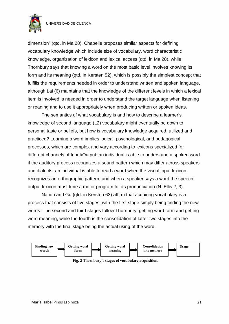
Nation and Gu (qtd. in Kersten 63) affirm that acquiring vocabulary is a
process that consists of five stages, with the first stage simply being finding the new
words. The second and third stages follow Thornbury; getting word form and getting
word meaning, while the fourth is the consolidation of latter two stages into the
memory with the final stage being the actual using of the word.
Finding new words
Getting word form
Getting word meaning
Consolidation into memory
Usage
Fig. 2 Thornbury’s stages of vocabulary acquisition.
María Isabel Pinos Espinoza 22
UNIVERSIDAD DE CUENCA
These stages may be conscious or unconscious; Nick Ellis suggests that
people are naturally active processors of information, and there are two compatible
hypotheses of how vocabulary is acquired: an implicit vocabulary learning hypothesis
which holds that “the meaning of a new word is acquired totally unconsciously as a
result of abstraction from repeated exposures in a range of contexts”, and an explicit
vocabulary learning hypothesis that holds that vocabulary acquisition can be
facilitated by the use of metacognitive strategies such as “(i) noticing that the word is
unfamiliar, (ii) making attempts to infer the word from context (or acquiring the
definition from consulting others or dictionaries or vocabularies), (iii) making attempts
to consolidate this new understanding by repetition and associational learning
strategies such as semantic or imagery mediation techniques” (5).
The two dissociable learning abilities used when learning vocabulary: the
natural, simple, unconscious process of implicit learning and the conscious,
controlled operation of explicit learning in which individuals look for structures that
allow them to test hypotheses should be both taken into account when teaching
vocabulary “…however vocabulary acquisition may be achieved, it can only enhance
the natural acquisition of language competence” (N. Ellis 10). Consequently when
teaching-learning vocabulary a variety of strategies such as inference from context,
use of dictionaries, collocations, guessing skills, etc. should be employed (N. Ellis 5,
6, 10). Coady (qtd. in Kersten 64) simplifies these ideas into three principles to be
taken into account when teaching vocabulary:
1. It is essential to provide definitional and contextual information about
words.
2. Motivate learners to process information about words at a deeper level.
3. Learners should have multiple exposures to a word.
These three principles are supported by many authors although Carter affirms
that the first vocabulary that a language learner acquires needs to be explicitly taught
because acquiring words incidentally (implicit learning) will only happen when the
learners have a certain repertoire of words at their disposal (qtd. in Kersten 68).
Schmitt reiterates this point by stating that vocabulary acquisition involves different
aspects of word knowledge which will be mastered at different stages of learning and
at different rates (qtd. in Ma 29).
María Isabel Pinos Espinoza 23
UNIVERSIDAD DE CUENCA
Vocabulary acquisition, be it implicit or explicit, requires time and practice,
thus it is an ongoing process which needs discipline, students need to work each day
in learning vocabulary in order to put new words in their long term memory
(Mehering 3). Nation and Waring stated that “learners need to encounter the word
multiple times in authentic speaking, reading, and writing context and the student’s
appropriate level” (qtd. in Mehering 3).
According to Mehering vocabulary needs to be learned through context in
order to make students understand the correct usage of a word avoiding misusing it
which usually happens when based exclusively on its dictionary meaning. To make
students learn vocabulary better it is important that they find the new words useful as
well as being able to use these new words more often when they are studying (4),
which seems to be one important reason to expose students to videos that contain
authentic language such as sitcoms.
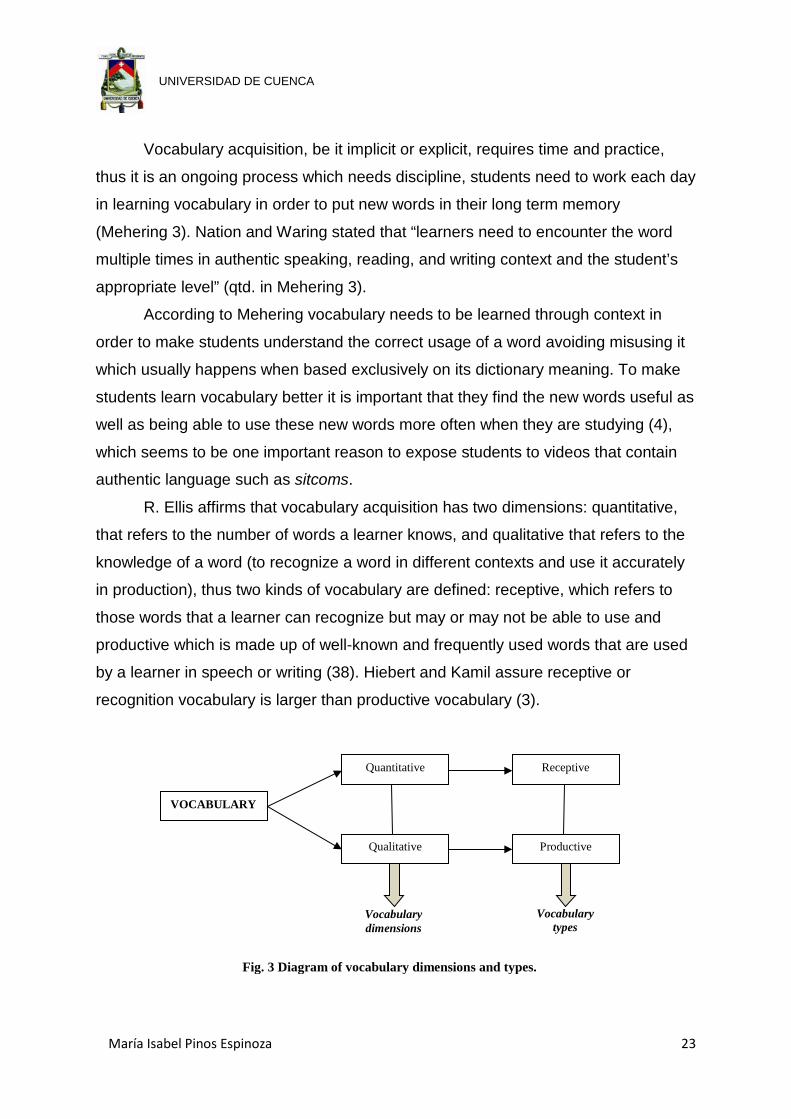
R. Ellis affirms that vocabulary acquisition has two dimensions: quantitative,
that refers to the number of words a learner knows, and qualitative that refers to the
knowledge of a word (to recognize a word in different contexts and use it accurately
in production), thus two kinds of vocabulary are defined: receptive, which refers to
those words that a learner can recognize but may or may not be able to use and
productive which is made up of well-known and frequently used words that are used
by a learner in speech or writing (38). Hiebert and Kamil assure receptive or
recognition vocabulary is larger than productive vocabulary (3).
Qualitative Productive
VOCABULARY
Quantitative Receptive
Vocabulary dimensions
Vocabulary types
Fig. 3 Diagram of vocabulary dimensions and types.

María Isabel Pinos Espinoza 24
UNIVERSIDAD DE CUENCA
1.1. VOCABULARY TEACHING
Vocabulary is a main part of language teaching, which unfortunately in the
teaching and learning process has usually been undervalued. For example, Howatt
and Rivers state that during the Grammar Translation Method (the first method to be
used in teaching a second language), students were given bilingual vocabulary lists
to learn in order to support them being able to translate long classical passages and
literary language samples with obsolete vocabulary were used, thus realistic
vocabulary was not taught (qtd. in Boyd 5-7). During the Reform Movement, which
started in the 1920s and emphasized the importance of oral communication and
phonetic training, vocabulary words taught in classes were associated with reality.
Furthermore, they were selected according to their simplicity and usefulness (Boyd
8).
Boyd mentions that the Direct Method brought interaction as the foundation
for natural language acquisition thus encouraging the use of the target language
without translations. For this reason, everyday vocabulary and sentences were used,
thus vocabulary was simple and familiar. It was explained through labeled pictures
and demonstrations for concrete vocabulary and the association of ideas were used
for abstract vocabulary. Charts, pictures and objects were also used to explain
meaning of words and the term realia or realien was adopted at this time (9).
During the 1920s and 1930s, the Reading Method began in the United States
and Situational Language Teaching in Great Britain, which aimed to develop reading
skills. For the first time it was considered that vocabulary was one of the most
important aspects of second language learning thus emphasis was placed on
“developing a scientific and rational basis for selecting the vocabulary content of
language courses” (Boyd 10).
The Audio Lingual Method considered language learning as a process of habit
formation, it paid systematic attention to pronunciation and intensive oral drilling of
basic sentence patterns, as a result vocabulary items were selected according to
their simplicity and familiarity and drills were used to introduce new words.
Unfortunately, language learners used to overvalue word knowledge equating it with
language knowledge (Boyd 11, 12).

María Isabel Pinos Espinoza 25
UNIVERSIDAD DE CUENCA
Boyd assures that the publication of Syntactic Structures by Noam Chomsky,
in 1957 was “a revolutionary reminder of the creativity of language and a challenge
to the behaviorist view of language as a set of habits”. Chomsky proposed an
autonomous linguistic competence in which the sociolinguistic and pragmatic factors
were the basis for effective language use (12). On the other hand, Dell Hymes
introduced the concept of communicative competence which was defined as the
“internalized knowledge of the situational appropriateness of language” (qtd. in Boyd
12).
As a result of Chomsky’s and Hymes’ models, language teaching changed
from focusing on command of structures to communicative proficiency, thus
Communicative Language teaching was established. According to Stern, the latter
had the objective of making language learners be in closer contact with the target
language encouraging fluency over accuracy (qtd. in Boyd 13). Although vocabulary
was extremely important to the point that Widdowson claimed that native speakers
are able to understand grammatically incorrect utterances if they have accurate
vocabulary rather than those ones with correct grammar and inaccurate vocabulary,
it was not the focus of the method itself or research (qtd. in Boyd 13). Larsen-
Freeman mentions that vocabulary teaching used real situations, contextualized
activities, which focused on the discourse; these aiming to give students the
opportunities to develop strategies for interpreting and using the language as it is
actually used by native speakers (qtd. in Boyd 14). Furthermore, Boyd sustains that
“since vocabulary development occurs naturally in L1 through contextualized, natural
sequenced language, it will develop with natural communicative exposure in L2”
(14).
Schmitt points out that during the late 70’s and early 80’s second language
acquisition research turned attention to how the learner’s actions may affect their
language acquisition. As a consequence, language teachers were motivated to
analyse successful language learners and their learning strategies, thus changing
from a teacher-centred to a student-centred methodology (qtd. in Lai 2).
Krashen and Terrel described the Natural Approach as a method designed
mainly with the objective of making a beginner student able to reach appropriate
levels of oral communicative ability in the language classroom. Thus it “emphasizes
María Isabel Pinos Espinoza 26
UNIVERSIDAD DE CUENCA
comprehensible and meaningful input rather than grammatically correct production”.
For the Natural Approach methodology, the acquisition of a new language happens
through the comprehension of vocabulary. Consequently the teaching of vocabulary
focuses on the use of important and relevant input in order to achieve true
vocabulary acquisition. The method also recommends reading as a means to
acquire new vocabulary (131-156).
Lai notes that traditional approaches of teaching a foreign language focused
on teaching vocabulary unsystematically in class leave students to learn the lexicon
on their own without much instruction; on the other hand current vocabulary
instruction is based on different learners´ needs, goals and learning styles, thus
words that students are expected to meet frequently are presented systematically.
Furthermore teachers are aware that vocabulary needs to be learned outside of the
classroom, thus encouraging students to know the different levels of knowing a
lexical item as well as teaching the different vocabulary learning strategies are the
teachers’ objectives. From the different vocabulary learning strategies, guessing
from context is considered to be the most useful. In this approach teachers use
partially or fully contextualized activities such as reading, listening, speaking and
writing in authentic communication activities (9).
Vocabulary teaching has changed from the direct teaching of vocabulary
during the grammar translation method to incidental vocabulary teaching in the
communicative approach, and currently to implicit and explicit learning. Teaching
independent learning strategies in order to make students learn vocabulary on their
own is essential for vocabulary teaching (qtd. in Lai 9, 10).
Nowadays vocabulary is considered as fundamental part of the second or
foreign language acquisition process (qtd. in Fazeli 177), it enables the learner to
communicate and understand the language in real situations.
Teaching vocabulary is essential in the learning process but a difficult task as
it requires students’ time, motivation and self-learning strategies. It seems to be that
this process becomes easier when the words taught are useful for the learner and
he/she can find them in use outside of the classroom. Thus, students may be able to
find words used in real contexts and situations when watching sitcoms; T.V.

María Isabel Pinos Espinoza 27
UNIVERSIDAD DE CUENCA
programs that, according to interviews with learners, they like and watch outside the
classroom.
1.2. VOCABULARY LEARNING STRATEGIES (VLS)
Rahimy and Kiana mention that students find it difficult to learn vocabulary as
they always forget whatever words they have memorized. In order to provide a
solution for this issue, research has been made in the field of Vocabulary Learning
(VL) with the objective of defining and analyzing different strategies used by students
to learn vocabulary (142). Thus, Siriwan affirms that language students will benefit
and become independent language learners if teachers introduce a great number of
VLS [Vocabulary Learning Strategies] to them because they will be able to select the
strategies that best suit their different learning needs (qtd. in Rahimy and Kiana 142).
Intaraprasert defines Vocabulary Learning Strategies (VLS) as "any set of
techniques or learning behaviors which language learners use to understand the
meaning of a new word, to restore the knowledge of newly-learned words, and to
expand one’s knowledge of vocabulary" (qtd. in Rahimy and Kiana 141). Cameron
simply defines VLSs as "the actions that learners take to help themselves
understand and remember vocabulary items", while Catalan expands on it to include
the different aims of vocabulary acquisition; "knowledge about the mechanisms
(processes, strategies) used in order to learn vocabulary as well as steps or actions
taken by students (a) to find out the meaning of unknown words, (b) to retain them in
long-term memory,(c) to recall them at will, and (d) to use them in oral or written
mode" (qtd. in Rahimy and Kiana 142).
The acquisition of lexical items is extremely important for L2 learners, thus a
considerable body of literature about VLSs has been developed by various authors.
For example, Schmitt classifies strategies into two groups; those used to define the
word’s meaning, known as discovery strategies, which include determination and
social strategies, and the consolidation strategies which are social and memory
strategies used to store the meaning of a word into the memory. Schmitt also affirms
that “using a bilingual dictionary, guessing from context, and asking classmates for
help were the most common discovery strategies, while verbal repetition, written
María Isabel Pinos Espinoza 28
UNIVERSIDAD DE CUENCA
repetition, and studying the spelling of the word were the most frequent consolidation
strategies” (qtd. in Winke and Abbuhl 698).
Alternatively, Cohen proposes strategies that deal with remembering words,
semantic strategies, and vocabulary learning and practicing strategies. Lawson and
Hoben propose individual vocabulary learning strategies which are: repetition, word
feature analysis, simple elaboration and complex elaboration (qtd. in Rahimy and
Kiana 143-145).
Winke and Abbuhl affirm that different authors and researchers mention Input-
Based strategies which are based on “listening to native speakers of the target
language, asking for a translation into the first language (L1), consulting reference
works in the L2, listening to various media (e.g., TV, radio), and reading as steps L2
learners take to learn more about target vocabulary”, this means that the learner is
looking for oral or written input in the target language in order to learn or remember
vocabulary (700).
Taking into account Winke and Abbuhl’s affirmation and the fact that learners
are usually in close contact with TV, it is possible to believe that TV programs can
help students to learn vocabulary.
Some authors also mention Output-based strategies which refer to “taking
notes, speaking with native speakers, engaging in oral or written rehearsal/repetition,
creating and maintaining a vocabulary notebook, and attaching English labels to
objects”, in these strategies, the learner is engaged in the use of L2 in written or oral
forms (Winke and Abbuhl 700). Furthermore, analyzing word meanings, using
association to remember words (such as associating an image with the new word),
guessing from context or common sense, planning one's course of study, monitoring
one's progress, and testing oneself are defined as cognition-based strategies (Winke
and Abbuhl 700).
1.3. VOCABULARY LEARNING
Do we need to learn vocabulary? The intuitive answer is, of course, yes. How
can we communicate or understand anything in a second or foreign language
without having the tools to do it? Schmitt suggests that the only way to truly
communicate is to have the appropriate lexicon to do so; between 8000 and 9000

María Isabel Pinos Espinoza 29
UNIVERSIDAD DE CUENCA
word families for written English, and 5000 to 7000 for spoken communication and
that the only true way to achieve this is to develop long-term programs which engage
learners with the lexical items to be learned (329).
What is understood by vocabulary learning? Siriwan defines vocabulary
learning as the process of learning a “collection or the total stock of words in a
language that are used in particular contexts" or “learning a package of sub-sets of
words as well as learning how to use strategies to cope with unknown or unfamiliar
words” (qtd. in Rahimy and Kiana 141).
There are many theories as to how students manage to learn vocabulary and
what actually the best method is. Many teachers, and textbooks are dedicated to the
idea that vocabulary should be learned in context (Prince 478) and we should move
away from the translation method. Prince himself questioned the validity of the idea,
above all because it had not been empirically proven (479). His research pointed to
several important factors, the most important being that learning strategies employed
by students of different levels differs considerably. Weaker students tended to rely
more heavily on direct translation, and when asked to perform such a task, were able
to outperform against more advanced students (485). However, Prince found that
while weaker students could remember this vocabulary, it remained isolated and
could not be transferred to other situations – when asked to provide the same words
in context, whereas students who were stronger could more easily adapt and use
new words (486). Prince suggests that one of the reasons for the disparity is the
sheer “cost” weaker students face when learning and using vocabulary in context – it
requires not only recall, but also syntactic elements (487). The overall effect of this
learning through translation, according to Prince is that when it comes to the transfer
of knowledge of the lexicon to productive situations, students are unable to do so
(489).
When it comes to vocabulary in context, there has been a lot of research;
Nation looked at the ability of students to guess vocabulary in context by replacing
real words with nonsense words, and found that on average, higher proficiency
students performed substantially better than low proficiency students and that the
number of unknown words in a text also affects students’ ability to guess vocabulary
in context (33). More recently, Nation looked at what vocabulary actually is; he broke

María Isabel Pinos Espinoza 30
UNIVERSIDAD DE CUENCA
vocabulary down into categories: High-frequency vocabulary, academic vocabulary,
technical vocabulary, and low frequency vocabulary (11-12). Almost 80% of
academic texts are made up of high frequency words of which around 77% are found
as the most common 1000 words in any corpus (16). Nation also suggests that on
average a good technical dictionary will contain 1000 specific words (12). In the end,
in order to be able to read with minimal disturbance a reader requires a vocabulary
of 15,000 to 20,000 words and so teachers should focus on teaching strategies for
learning and remembering vocabulary (20).
“Guessing from context is probably one of the most useful skills learners can
acquire and apply both inside and outside the classroom. What’s more, it seems to
be one that can be taught and implemented relatively easily. It is also one that we all
already use – perhaps unconsciously – when reading and listening in our mother
tongue” (Harmer 148).
Learning vocabulary in context is defined as “…the active, deliberate
acquisition of a meaning for a word in a text by reasoning from context, without
external sources of help such as dictionaries or people.”(Rapaport 1). That having
been said, Rapaport goes on to argue that the “context” itself has to be much more
broadly defined to include a network of factors including background knowledge, the
situation (written or visual), and internalization of the situation (perhaps incorrectly)
(12-15). As Clarke and Silberstein said in Birch, it is extremely important that
students are aware of the different clues available to them when they cannot
recognize a word. They should realize they can continue reading the text and
understand the unfamiliar word; above all students need to be taught situations in
which the meaning of a particular word or phrase is not essential to understand a
passage (129).
The question still remains as to how we can teach, or at least use, specific
methodologies in the classroom. The most important step is to choose what
vocabulary has to be learned, how it should be learned and how we are going to
assess it. Nation and Chung believe teachers need to concentrate on the high
frequency words – again suggesting that the first 1000 high frequency words are the
most important, followed by academic and technical words, suggesting that technical
María Isabel Pinos Espinoza 31
UNIVERSIDAD DE CUENCA
words have been underestimated in their importance, between 30 and 20% of
running text may be technical words in a technical text (543-546).
Sonbul and Schmir found that direct teaching of vocabulary to be more
effective in helping students learn and assimilate vocabulary than reading alone
(253), but can other media, such as video help students learn vocabulary? Tschirner
believes that with the advent of broadband internet and sites such as Youtube, it is
inevitable that these resources should be used to provide students with rich
language inputs (25) and suggests some practical criteria to use when choosing the
videos you wish to use: Short enough that they can be seen several times, yet long
enough to engage the students and be selected for relevance, validity, and the
quantity and quality of linguistic input.(34-35). Other studies developed by White,
Easton and Anderson of the use of video have found that students, when left to
choose when to watch a video related to a lesson will choose it first to help them
become acquainted with the context of the new lesson (167). Furthermore, the use
of video as integral parts of classroom based instruction is being put forward by
some for learning vocabulary and developing comprehension and has been found to
help learners of all levels (Hall and Dougherty Stahl 403; Lin 199)
1.4. VOCABULARY ASSESSMENT
Read affirms that vocabulary assessment can be a simple activity that consists
of selecting a suitable number of target words and assessing if they are known by
the use of established test formats such as multiple choice, gap filling, matching or
some form of translation; these tests are widely used in second language teaching
for different purposes, and if they are correctly designed, they can be an important
and efficient tool to measure learners’ competence (106).
One area of vocabulary assessment is the measurement of vocabulary size,
which is known as breadth of vocabulary knowledge and it aims to determine the
number of words known by the use of word frequency lists. A second area that is
generally used to assess is the depth of vocabulary knowledge which focuses on
assessing how well a particular word is known by the use of word associates formats
with the Vocabulary Knowledge Scale (Read 106). Lessard-Clouston (186) mention
that depth of vocabulary includes a person's knowledge about the quality of a word
María Isabel Pinos Espinoza 32
UNIVERSIDAD DE CUENCA
including a word's sound pattern, referential meanings, affixes, function in the
grammar, collocational restrictions, register, dialectical restrictions, idiomatic uses,
metaphorical extensions, synonyms, anonyms, and hyponyms, and graphic forms.
Depth of a lexical item in the mental lexicon not only specifies the word's meaning
but also refers to the "morphology, phonology, syntax, sociolinguistic aspects,
differences between written and spoken uses, and strategies for approaching
unknown words" (Bromley 529).
The assessing of vocabulary breadth has been a longstanding area of research
because the size of vocabulary knowledge has closely been associated with the
reading comprehension ability, and for L2 learners this type of assessment “can
reveal the extent of the lexical gap they face in coping with authentic reading
materials and undertaking other communicative tasks in the target language” (Read
107).
“Vocabulary size measures typically require a relatively large sample of words
that represent a defined frequency range, together with a sample response tasks to
indicate whether each word is known or not” (Read 107).
Read states that there are different vocabulary size tests such as the General
Service List (GSL) developed by West in 1953, which contains a selection of 2000
high frequency word families that can be found in any written or spoken English text
but it has been criticized as contains outmoded entries and the lack of modern terms.
The Academic Word List (AWL) developed by Coxhead in 2000 combine criteria of
frequency, range, familiarity and pedagogy, it contains 570 word families which can
frequently be found in written texts across a range of university disciplines, thus it
has been widely used in teaching and testing English for academic purposes (108).
Read also affirms that more work is still needed in order to develop a well-formulated
word list that can be used to measure the vocabulary size, therefore an alternative
approach is to rely on the judgment of a language teachers or other linguistic experts
(109, 110).
Nation’s Vocabulary Level tests and Vocabulary Size Test are the most widely
used measure of English vocabulary size for second language learners. The tests
contain two types of questions: matching words with their synonyms or short
definitions, or a multiple choice format that presents each target word in a short non-

María Isabel Pinos Espinoza 33
UNIVERSIDAD DE CUENCA
defining sentence followed by four definitions as options. These kinds of questions
provide evidence that the target words are actually known (Read 110).
Fig. 4 Example of Vocabulary level test proposed by Nation.
Other vocabulary size tests are those that use the Yes/No format (checklist).
A series of words are presented and the test taker needs to indicate whether he/she
knows each word or not, thus the honesty of the test taker is extremely important.
These kinds of tests are usually used as placement tests or as a general
measurement of breadth in vocabulary or competence in the language. The Yes/No
format has been proved to be effective for assessing the state of learner’s
vocabulary knowledge (Read 110-113).

María Isabel Pinos Espinoza 34
UNIVERSIDAD DE CUENCA
Fig. 5 Example from the Vocabulary Level Test proposed by Nation.
The measurement of vocabulary quality or depth focuses on analyzing the
knowledge of words as functional units in the learner’s L2 lexicon; pronunciation and
spelling of a word, its morphological forms, syntactic functions, frequency, and its
correct use from a sociolinguistic perspective and so on. It is generally agreed that
assessing all that learners may know about a particular set of words is not
necessary; on the contrary measures that focus on selective key aspects of word
knowledge are widely used. Furthermore, there is no consensus of what aspects of
word knowledge are the most important and which of them should be assessed in
standardized tests (Read 113, 114).
The vocabulary tests that have been mentioned, present the target words as
isolated lexical units with no reference to context. Hyland and Tse affirm that
“learners should engage with the actual use of lexical items in specific contexts if
they are to be successful language users in the academic environment or elsewhere”
(qtd. in Read 115).
Read’s word association format has been extensively adopted in order to test
deep word knowledge in a meaningful way. The test is built on the concept of word
association assessing key elements of the core meaning of the target word, or
alternatively more than one meaning of the word (Read 113).
María Isabel Pinos Espinoza 35
UNIVERSIDAD DE CUENCA
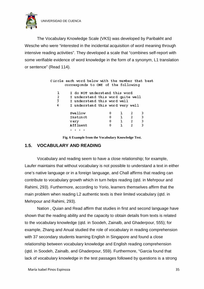
The Vocabulary Knowledge Scale (VKS) was developed by Paribakht and
Wesche who were “interested in the incidental acquisition of word meaning through
intensive reading activities”. They developed a scale that “combines self-report with
some verifiable evidence of word knowledge in the form of a synonym, L1 translation
or sentence” (Read 114).
Fig. 6 Example from the Vocabulary Knowledge Test.
1.5. VOCABULARY AND READING
Vocabulary and reading seem to have a close relationship; for example,
Laufer maintains that without vocabulary is not possible to understand a text in either
one’s native language or in a foreign language, and Chall affirms that reading can
contribute to vocabulary growth which in turn helps reading (qtd. in Mehrpour and
Rahimi, 293). Furthermore, according to Yorio, learners themselves affirm that the
main problem when reading L2 authentic texts is their limited vocabulary (qtd. in
Mehrpour and Rahimi, 293).
Nation , Quian and Read affirm that studies in first and second language have
shown that the reading ability and the capacity to obtain details from texts is related
to the vocabulary knowledge (qtd. in Soodeh, Zainalb, and Ghaderpour, 555); for
example, Zhang and Anual studied the role of vocabulary in reading comprehension
with 37 secondary students learning English in Singapore and found a close
relationship between vocabulary knowledge and English reading comprehension
(qtd. in Soodeh, Zainalb, and Ghaderpour, 559). Furthermore, “Garcia found that
lack of vocabulary knowledge in the test passages followed by questions is a strong

María Isabel Pinos Espinoza 36
UNIVERSIDAD DE CUENCA
element influencing fifth and sixth grade of Latino bilingual learners on a test of
reading comprehension” (qtd. in Soodeh, Zainalb, and Ghaderpour, 559). Nagy
affirms that “vocabulary knowledge positively affects reading comprehension, and
instruction needs to be multifaceted” (qtd. in Mehrpour and Rahimi, 294).
It seems then that vocabulary size and knowledge of meanings have a direct
influence in the reading comprehension ability; thus when the main teaching
objective is making students into proficient readers, vocabulary teaching should be a
priority.
1.6. TEACHING VOCABULARY WITH VIDEOS
A textbook is generally the main material used in a traditional language
classroom but with the invention of computers media-based materials, such as
videos, have been broadly introduced into the language classrooms with the
objective of promoting traditional language learning to a holistic and multi-sensory
level. Researchers have suggested that learning was facilitated when visual and
audio representations co-occurred in a person's working memory. Mayer and
Moreno maintain that “in order to meaningfully comprehend a text in a multimedia
format, learners select relevant pictorial and linguistic information, organize the input
into coherent visual and verbal mental representations, and construct referential
connections between the two” (qtd. in Wang 218). Wang affirms that empirical
studies have shown that language learning is enhanced by the use of pictures and
translations. As well as the effects of visual and audio aids on L2 vocabulary
learning, the studies also manifested “the capacity theory that could be explained as
pictures and sounds bridging the gap of unconnected themes, saving spaces for
learners' working memory and eventually speeding up the process of
comprehension” (218). Furthermore, Brett, Egbert &Jessup, and Khalid have
demonstrated strong evidence that multimedia has rich and authentic
comprehensible input which positively affects language learning (qtd. in Harji, Woods
and Alabi 38).
Harji, Woods and Alabi sustain that multimedia technology aims to integrate
real-life situations with the target language into the classroom; in this atmosphere

María Isabel Pinos Espinoza 37
UNIVERSIDAD DE CUENCA
students are exposed to authentic environment of the target language which helps
them to expand their language acquisition (37).
Video is a multimedia tool that is widely used in language classes since it
seems to be more convenient, entertaining, and generally very handy. Furthermore,
empirical studies have confirmed the positive effect of visual and audio aids on L2
vocabulary learning as well as the use of pictures and translations (Wang 217, 218).
Canning-Wilson found that lexical learning which provided the learners with
immediate meaning in terms of vocabulary recognition can be reinforced through
images contextualized in video. Likewise, Hoogeveen proposes that the use of
videos might help learners to interact with the information with more personal
feelings instead of just receiving it and turning learning into a more fun and happier
process (qtd. in Wang 217).
Wang performed a study with twenty-eight Taiwanese EFL adult learners in
the process of implementing American TV drama in L2 vocabulary learning from
learners' perspectives. The results show that TV drama has a facilitative role in
learning new vocabulary; additionally learners confirm that the interest level and the
content’s familiarity play an important role in the process of learning as well as the
images, subtitles and repetition helped participants to "remember" the target words.
Other factors which contribute to the learning of the L2 vocabulary are the
authenticity of the language, the contextual meaning of the words, and dramatic
performances (217).
But what is it understood by “video”? Sherman defines video as the selection
and sequence of messages in an audio-visual context which contextualized the
learning process because teachers are able to introduce any aspects of real life into
the classroom (qtd. in Wang 219). On the other hand, Wang defines video as a
multimedia tool that helps to display content as well as to enhance lexical and
grammatical learning through the combination of sounds, images, and sometimes
texts, together with the socio-cultural information about human acts, traditions, living
styles, and their thinking patterns. Videos can be instructional, specifically created
with teaching purposes, or authentic, such as films, TV series, or commercials which
are created for native speakers of the target language. Through the use of videos,
which have a combination of visual and audio aids, messages are clarified and

María Isabel Pinos Espinoza 38
UNIVERSIDAD DE CUENCA
language points enhanced, they provide more rooms for learners’ working memory
capacity and lead to more successful retention of new information. Additionally,
videos have social cultural messages that allow learners to experience the real use
of the target language (219).
Videos can be used with subtitles. In fact, different studies affirm “the aspect
that the use of subtitles causes multisensory processing, interacting with audio,
video and print mechanisms. These information input foundations make the process
of language learning enhanced, improve the comprehension of the content, and
increase vocabulary by looking at the subtitled words in meaningful and stimulating
circumstances”(qtd. in Harji, Woods and Alabi 38). The findings of a study conducted
by Neuman support the impact of the use of subtitles on bilingual students'
acquisition of language, literacy, and conceptual knowledge. Neuman and Koskinen
also sustain that the use of subtitles influences ESL students’ acquisition of
vocabulary and reading development because they provide powerful comprehensible
input. Bean and Wilson reported that students who viewed L2 subtitled materials
showed significant improvement in reading comprehension, listening
comprehension, vocabulary acquisition, and word recognition (qtd. in Harji, Woods
and Alabi 39).
Harji, Woods and Alabi performed a study on the effectiveness on English
subtitles on the EFL learner’s vocabulary learning with 92 Iranian participants
randomly assigned to control and treatment groups; “the findings show that
participants viewing the videos with subtitles could obtain a significantly higher mean
score of the CST vocabulary tests than those who viewed the videos without
subtitles” (37).
The authors mentioned in this theoretical framework agree that vocabulary
learning is a complex interplay of different factors which means that the teaching
process needs to be carefully analyzed, thought out and planned in order to achieve
objectives which in turn must be defined according to students’ needs. This review
has also established a strong link between vocabulary knowledge and reading
comprehension, as well as the usefulness of videos for vocabulary learning.
Research into amalgamating the aforementioned areas is therefore justified.

María Isabel Pinos Espinoza 39
UNIVERSIDAD DE CUENCA
CHAPTER II RESEARCH METHODOLOGY
In order to carry out this dissertation within a theoretical-applied research
approach, pre-tests and post-tests were applied without a control group. Quantitative
and qualitative methods were used for the research; instruments such as
questionnaires, pre-test, post-test, interviews, teacher’s journal were used for data
gathering.
2.1. PARTICIPANTS
A sample of 22 students from the first level of the school of Early Stimulation,
which is part of the Faculty of Philosophy of the private University of Azuay,
participated in this research. The group was made up of 20 female and 2 male
students. Most of them consider it important to learn English as they believe they
will have better professional opportunities; others learn English because it is
mandatory for graduation in University of Azuay. The age of the students varies from
18 to 24 years old and most of them consider themselves having an English level of
beginners. The majority of participants affirmed that they were in contact with English
outside the classroom for one hour a week. They affirmed being in contact with the
language mainly by watching TV series or movies, listening to music, attending
private lessons and using the internet (chat and mail) but they do not use the
languge with friends or family.
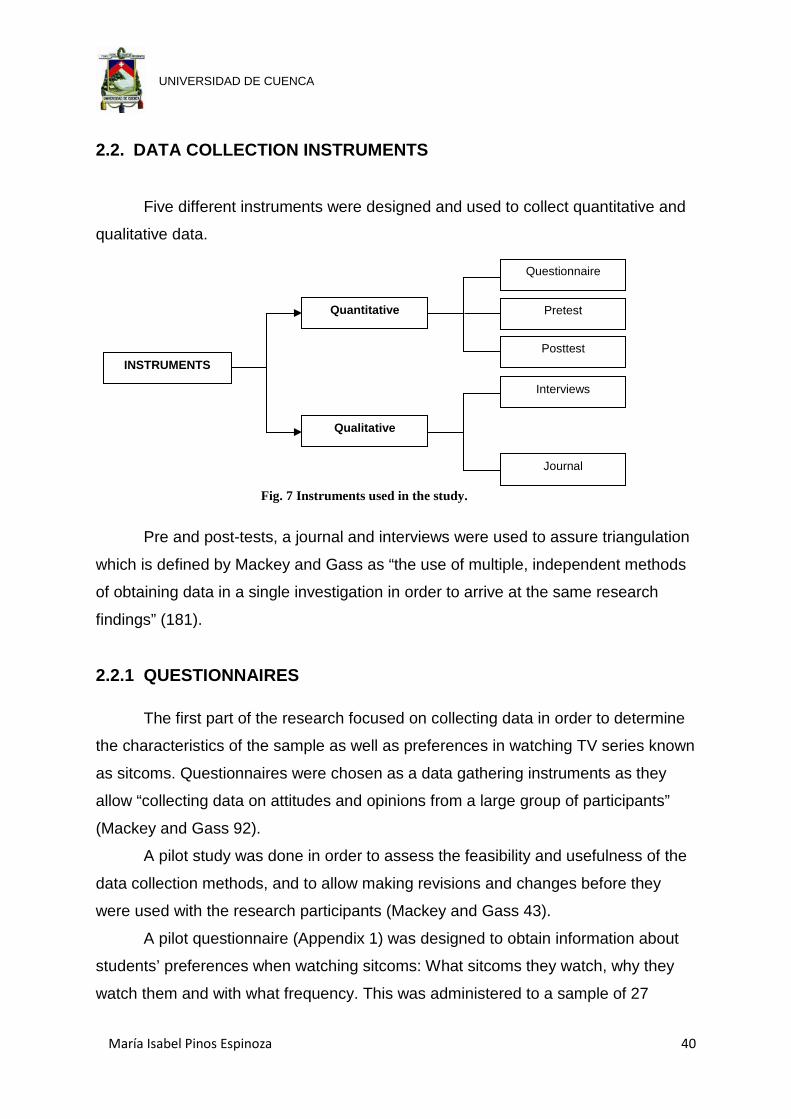
María Isabel Pinos Espinoza 40
UNIVERSIDAD DE CUENCA
2.2. DATA COLLECTION INSTRUMENTS
Five different instruments were designed and used to collect quantitative and
qualitative data.
Pre and post-tests, a journal and interviews were used to assure triangulation
which is defined by Mackey and Gass as “the use of multiple, independent methods
of obtaining data in a single investigation in order to arrive at the same research
findings” (181).
2.2.1 QUESTIONNAIRES
The first part of the research focused on collecting data in order to determine
the characteristics of the sample as well as preferences in watching TV series known
as sitcoms. Questionnaires were chosen as a data gathering instruments as they
allow “collecting data on attitudes and opinions from a large group of participants”
(Mackey and Gass 92).
A pilot study was done in order to assess the feasibility and usefulness of the
data collection methods, and to allow making revisions and changes before they
were used with the research participants (Mackey and Gass 43).
A pilot questionnaire (Appendix 1) was designed to obtain information about
students’ preferences when watching sitcoms: What sitcoms they watch, why they
watch them and with what frequency. This was administered to a sample of 27
INSTRUMENTS
Qualitative
Quantitative
Questionnaire
Pretest
Posttest
Interviews
Journal
Fig. 7 Instruments used in the study.

María Isabel Pinos Espinoza 41
UNIVERSIDAD DE CUENCA
students who were taking a first English level summer course at the University of
Azuay. The sample included male and female students whose ages range of
between 18 to 22 years old. The main objective of the questionnaire was “to gather
information that learners are able to report about themselves” (Mackey and Gass
92). Furthermore, the pilot questionnaire was used in order to test the questions,
language construction and its layout.
The questionnaire was administered in the L1 (Spanish) in order to minimize
any bias that may arise from misunderstandings or difficulty in answering questions
and obtain accurate information while avoiding participant boredom. Questions 1, 2
and 3 were closed-item (table 1) and there were four open-ended questions (3, 4, 5
and 7), as shown in table 2, which were used in order to guide hypothesis formation.
Question number two was used as a filter in order to determine whether or not the
participants were qualified to continue answering.
1. ¿Usted usualmente mira comedias de situaciones cuyo lenguaje original es inglés?
SI NO
2. ¿Con qué frecuencia mira comedias de situaciones?
Nunca una vez por semana dos o más veces por semana
6. ¿Le gustaría que las comedias de situaciones que menciona en este cuestionario sean
utilizadas en las clases de inglés?
SI NO
Fig. 8 Examples of closed-item questions used in the pilot questionnaire.
3. Por favor escriba que comedias de situaciones usted mira.
4. ¿Cuál es su favorita?
5. Por favor escriba tres razones del porqué le gusta mirar comedias de situaciones
7. Si su respuesta es SI a la pregunta anterior, por favor escriba una razón del porqué de su
respuesta.
Fig. 9 Examples of open-ended questions used in the pilot questionnaire.
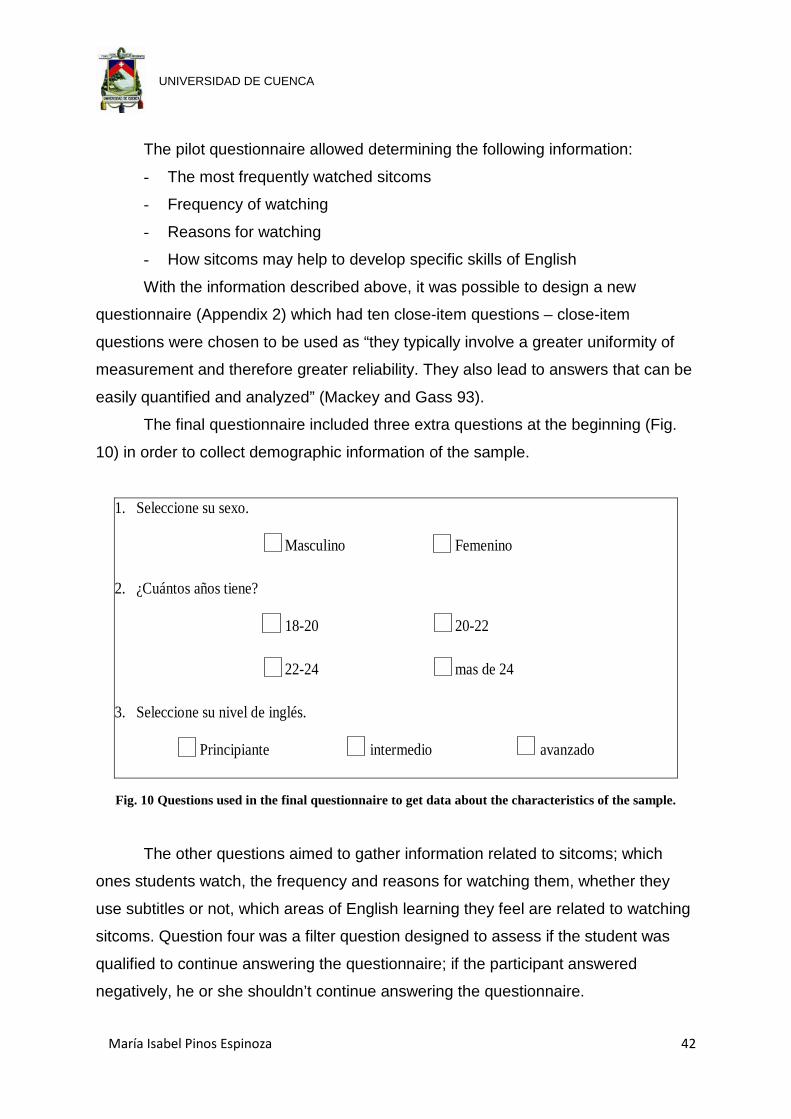
María Isabel Pinos Espinoza 42
UNIVERSIDAD DE CUENCA
The pilot questionnaire allowed determining the following information:
- The most frequently watched sitcoms
- Frequency of watching
- Reasons for watching
- How sitcoms may help to develop specific skills of English
With the information described above, it was possible to design a new
questionnaire (Appendix 2) which had ten close-item questions – close-item
questions were chosen to be used as “they typically involve a greater uniformity of
measurement and therefore greater reliability. They also lead to answers that can be
easily quantified and analyzed” (Mackey and Gass 93).
The final questionnaire included three extra questions at the beginning (Fig.
10) in order to collect demographic information of the sample.
1. Seleccione su sexo.
Masculino Femenino
2. ¿Cuántos años tiene?
18-20 20-22 22-24 mas de 24
3. Seleccione su nivel de inglés.
Principiante intermedio avanzado
Fig. 10 Questions used in the final questionnaire to get data about the characteristics of the sample.
The other questions aimed to gather information related to sitcoms; which
ones students watch, the frequency and reasons for watching them, whether they
use subtitles or not, which areas of English learning they feel are related to watching
sitcoms. Question four was a filter question designed to assess if the student was
qualified to continue answering the questionnaire; if the participant answered
negatively, he or she shouldn’t continue answering the questionnaire.

María Isabel Pinos Espinoza 43
UNIVERSIDAD DE CUENCA
This first questionnaire was used to gather information about sitcoms, which
was later used in the treatment.
PILOT QUESTIONNAIRE
FINAL QUESTIONNAIRE
Number of questions 7 10 Closed-item questions 3 10 Open-ended questions 4 0 Questions related to characteristics of the sample
0 3
Questions related to frequency of watching sitcoms
1 2
Questions related to sitcoms and their influence in learning English
1 2
Questions related to the use of subtitles
0 1
Fig. 11 Differences between the pilot and final questionnaires
A second demographics questionnaire (Appendix 3) was designed and
administered in order to gather more specific information about the characteristics of
the sample: reasons for learning English, frequency of contact with the language
outside the classroom as well as time dedicated to learn or practice English outside
the classroom. It was important to collect this data as it could affect the results of the
treatment.
This questionnaire included seven questions, five of them closed-item and two
opened-ended.
2.2.2 PRE AND POST TESTS
Mackey and Gass affirm that pre and post tests are used to measure the
immediate effect of the treatment and to what extent a treatment truly resulted in
learning (149).
The tests (Appendix 4) were designed in order to measure two aspects that
involve receptive vocabulary which are closely related to reading comprehension
ability: size (breadth) of vocabulary and meaning in context. Furthermore, the tests
also measured reading comprehension ability as it involves vocabulary recognition
and comprehension; as Read affirms this type of assessment “can reveal the extent
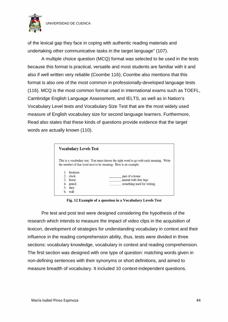
María Isabel Pinos Espinoza 44
UNIVERSIDAD DE CUENCA
of the lexical gap they face in coping with authentic reading materials and
undertaking other communicative tasks in the target language” (107).
A multiple choice question (MCQ) format was selected to be used in the tests
because this format is practical, versatile and most students are familiar with it and
also if well written very reliable (Coombe 116); Coombe also mentions that this
format is also one of the most common in professionally-developed language tests
(116). MCQ is the most common format used in international exams such as TOEFL,
Cambridge English Language Assessment, and IELTS, as well as in Nation’s
Vocabulary Level tests and Vocabulary Size Test that are the most widely used
measure of English vocabulary size for second language learners. Furthermore,
Read also states that these kinds of questions provide evidence that the target
words are actually known (110).
Fig. 12 Example of a question in a Vocabulary Levels Test
Pre test and post test were designed considering the hypothesis of the
research which intends to measure the impact of video clips in the acquisition of
lexicon, development of strategies for understanding vocabulary in context and their
influence in the reading comprehension ability, thus, tests were divided in three
sections: vocabulary knowledge, vocabulary in context and reading comprehension.
The first section was designed with one type of question: matching words given in
non-defining sentences with their synonyms or short definitions, and aimed to
measure breadth of vocabulary. It included 10 context-independent questions.

María Isabel Pinos Espinoza 45
UNIVERSIDAD DE CUENCA
9. REMEDY: We found a good remedy.
a. way to improve health b. way to prepare food c. rule about numbers d. place to eat in public
10. UPSET: I am upset.
a. Unhappy b. Rich c. Famous d. Tired
Fig. 13 Examples of questions used in the first section of pre and post-tests.
The second section included ten content dependent questions which were
used to measure the ability of using context clues to match a word given in a
sentence with its correct meaning.
1. Jennifer implied that she wanted to be Jim's girlfriend, but she didn't say so directly.
a. inferred b. declared c. refused d. questioned
2. The principal is extremely popular with the students because he is a strong advocate of students' rights.
a. opponent b. enemy c. member d. supporter
Fig. 14 Examples of questions used in the second section of pre and post-tests.
The first and second sections of the tests cover vocabulary appropriate to A1
and A2 level on the Common European Framework of Reference (CEFR), which
was selected from international vocabulary lists and include exclusively receptive
vocabulary (words that the student is expected to understand but which are not the
focus of a question) and productive vocabulary (words that the student needs to

María Isabel Pinos Espinoza 46
UNIVERSIDAD DE CUENCA
know in order to answer a question). The vocabulary students learn according to the
level’s syllabus was not used to avoid bias in the research and prevent external input
influencing the results.
The third section aimed to measure the reading comprehension competence,
it was designed based on the Diagnostic Assessment of Reading Comprehension
(DARC) Test structure, which “is an experimental test that involves reading
passages of three sentences, but it is specifically designed to control for the level of
decoding that is required” (Fletcher 326).
The different questions and reading were chosen from exercises used for
preparation for the Key English Test (KET), which is a basic level qualification that
shows people can use English to communicate in simple situations and belongs to
A2 level of the Common European Framework.
Fig. 15 Common European Framework Levels and their
corresponding international tests.
The posttest included the same sections and questions, the latter were
arranged in different order to guarantee the comparability of results.
2.2.3 STRUCTURED INTERVIEWS
Structured interviews were used to collect data of students’ perceptions and
feelings about the treatment; they allowed collecting data that was not directly
observable. Seidman states that these types of interviews aim to understand the
experience of other people and the meaning they make of that experience (qtd. in
Sahragard 263).
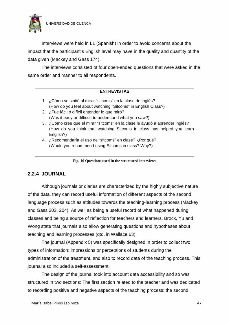
María Isabel Pinos Espinoza 47
UNIVERSIDAD DE CUENCA
Interviews were held in L1 (Spanish) in order to avoid concerns about the
impact that the participant’s English level may have in the quality and quantity of the
data given (Mackey and Gass 174).
The interviews consisted of four open-ended questions that were asked in the
same order and manner to all respondents.
ENTREVISTAS
1. ¿Cómo se sintió al mirar “sitcoms” en la clase de inglés? (How do you feel about watching “Sitcoms” in English Class?)
2. ¿Fue fácil o difícil entender lo que miró? (Was it easy or difficult to understand what you saw?)
3. ¿Cómo cree que el mirar “sitcoms” en la clase le ayudó a aprender inglés? (How do you think that watching Sitcoms in class has helped you learn English?)
4. ¿Recomendaría el uso de “sitcoms” en clase? ¿Por qué? (Would you recommend using Sitcoms in class? Why?)
Fig. 16 Questions used in the structured interviews
2.2.4 JOURNAL
Although journals or diaries are characterized by the highly subjective nature
of the data, they can record useful information of different aspects of the second
language process such as attitudes towards the teaching-learning process (Mackey
and Gass 203, 204). As well as being a useful record of what happened during
classes and being a source of reflection for teachers and learners, Brock, Yu and
Wong state that journals also allow generating questions and hypotheses about
teaching and learning processes (qtd. in Wallace 63).
The journal (Appendix 5) was specifically designed in order to collect two
types of information: impressions or perceptions of students during the
administration of the treatment, and also to record data of the teaching process. This
journal also included a self-assessment.
The design of the journal took into account data accessibility and so was
structured in two sections: The first section related to the teacher and was dedicated
to recording positive and negative aspects of the teaching process; the second
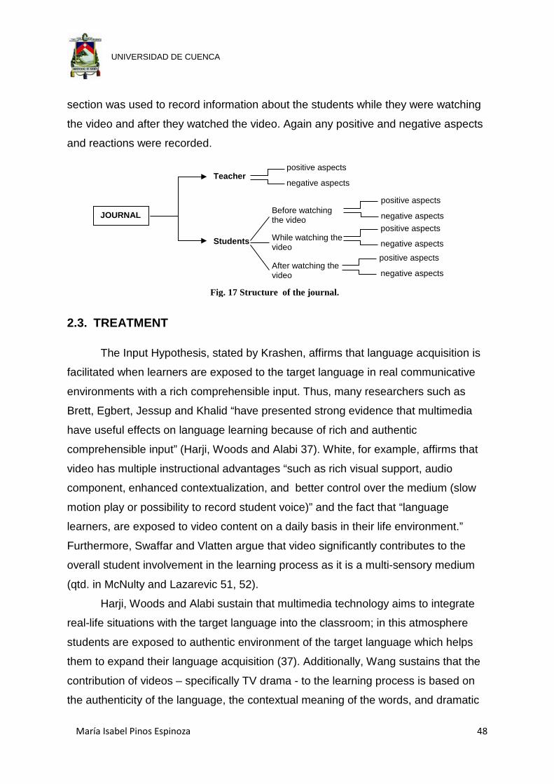
María Isabel Pinos Espinoza 48
UNIVERSIDAD DE CUENCA
section was used to record information about the students while they were watching
the video and after they watched the video. Again any positive and negative aspects
and reactions were recorded.
2.3. TREATMENT
The Input Hypothesis, stated by Krashen, affirms that language acquisition is
facilitated when learners are exposed to the target language in real communicative
environments with a rich comprehensible input. Thus, many researchers such as
Brett, Egbert, Jessup and Khalid “have presented strong evidence that multimedia
have useful effects on language learning because of rich and authentic
comprehensible input” (Harji, Woods and Alabi 37). White, for example, affirms that
video has multiple instructional advantages “such as rich visual support, audio
component, enhanced contextualization, and better control over the medium (slow
motion play or possibility to record student voice)” and the fact that “language
learners, are exposed to video content on a daily basis in their life environment.”
Furthermore, Swaffar and Vlatten argue that video significantly contributes to the
overall student involvement in the learning process as it is a multi-sensory medium
(qtd. in McNulty and Lazarevic 51, 52).
Harji, Woods and Alabi sustain that multimedia technology aims to integrate
real-life situations with the target language into the classroom; in this atmosphere
students are exposed to authentic environment of the target language which helps
them to expand their language acquisition (37). Additionally, Wang sustains that the
contribution of videos – specifically TV drama - to the learning process is based on
the authenticity of the language, the contextual meaning of the words, and dramatic
JOURNAL
Teacher
Students negative aspects
negative aspects
positive aspects
negative aspects
positive aspects
negative aspects Before watching the video
After watching the video
While watching the video
positive aspects
positive aspects
Fig. 17 Structure of the journal.
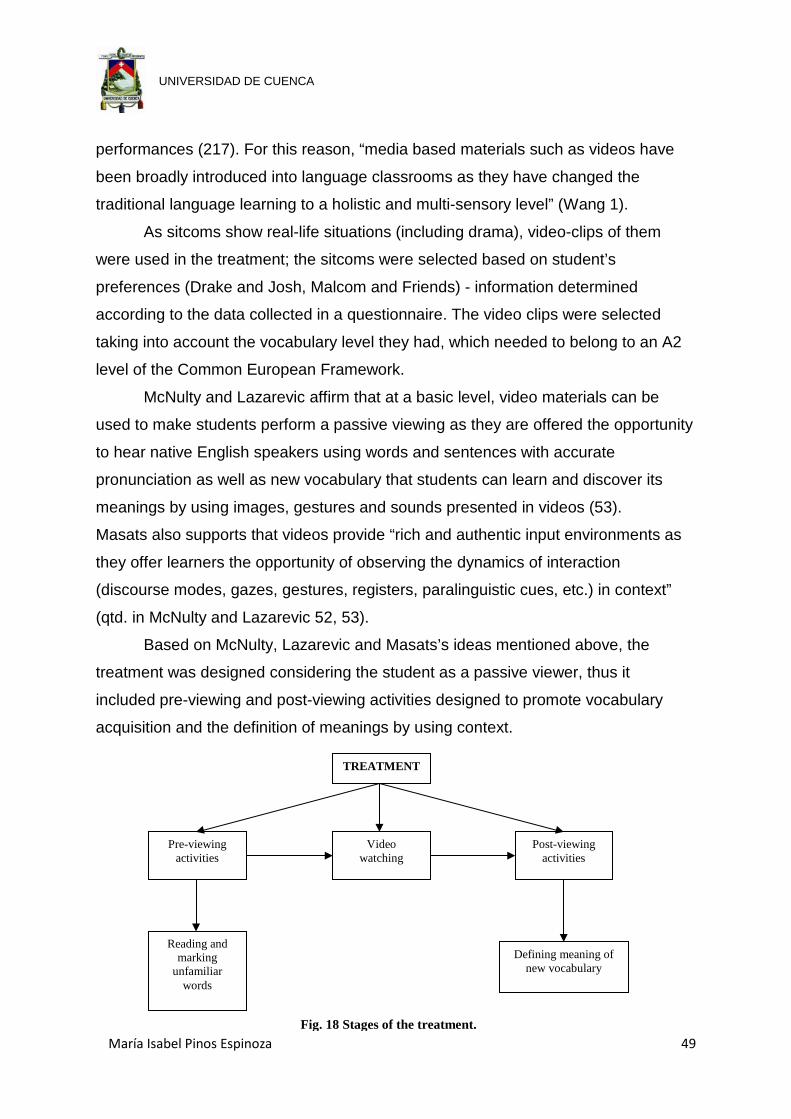
María Isabel Pinos Espinoza 49
UNIVERSIDAD DE CUENCA
performances (217). For this reason, “media based materials such as videos have
been broadly introduced into language classrooms as they have changed the
traditional language learning to a holistic and multi-sensory level” (Wang 1).
As sitcoms show real-life situations (including drama), video-clips of them
were used in the treatment; the sitcoms were selected based on student’s
preferences (Drake and Josh, Malcom and Friends) - information determined
according to the data collected in a questionnaire. The video clips were selected
taking into account the vocabulary level they had, which needed to belong to an A2
level of the Common European Framework.
McNulty and Lazarevic affirm that at a basic level, video materials can be
used to make students perform a passive viewing as they are offered the opportunity
to hear native English speakers using words and sentences with accurate
pronunciation as well as new vocabulary that students can learn and discover its
meanings by using images, gestures and sounds presented in videos (53).
Masats also supports that videos provide “rich and authentic input environments as
they offer learners the opportunity of observing the dynamics of interaction
(discourse modes, gazes, gestures, registers, paralinguistic cues, etc.) in context”
(qtd. in McNulty and Lazarevic 52, 53).
Based on McNulty, Lazarevic and Masats’s ideas mentioned above, the
treatment was designed considering the student as a passive viewer, thus it
included pre-viewing and post-viewing activities designed to promote vocabulary
acquisition and the definition of meanings by using context.
TREATMENT
Pre-viewing activities
Post-viewing activities
Video watching
Reading and marking
unfamiliar words
Defining meaning of new vocabulary
Fig. 18 Stages of the treatment.
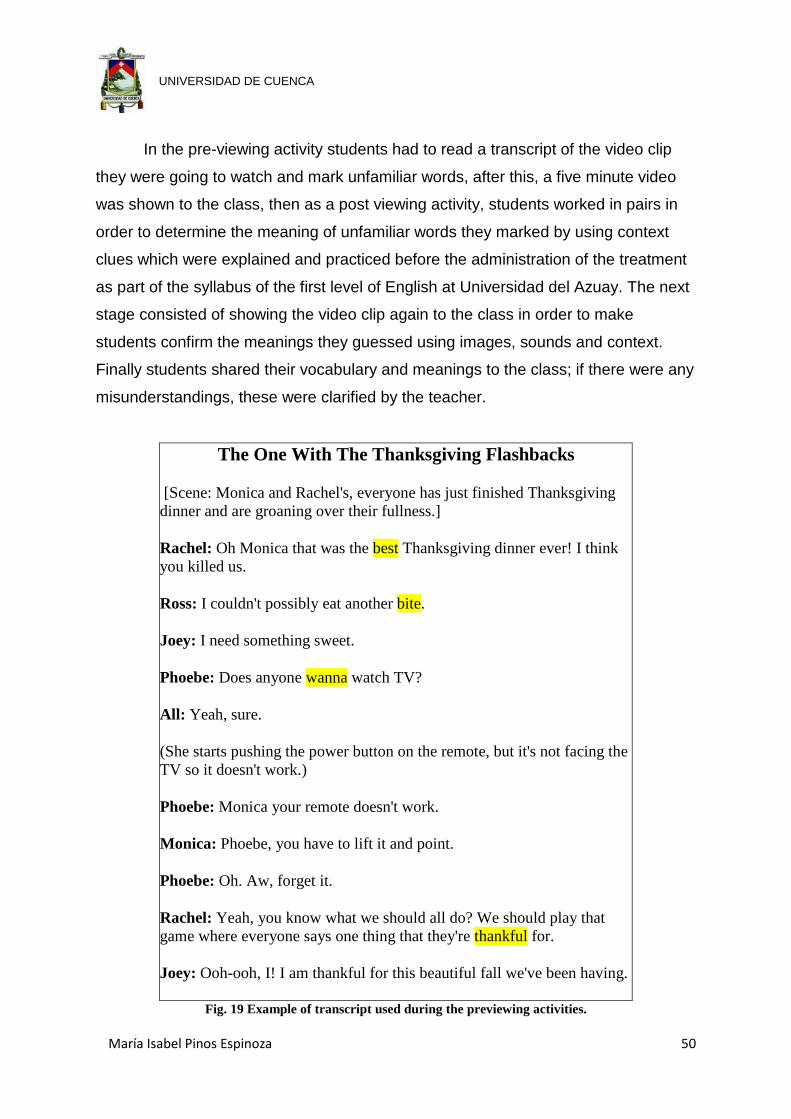
María Isabel Pinos Espinoza 50
UNIVERSIDAD DE CUENCA
In the pre-viewing activity students had to read a transcript of the video clip
they were going to watch and mark unfamiliar words, after this, a five minute video
was shown to the class, then as a post viewing activity, students worked in pairs in
order to determine the meaning of unfamiliar words they marked by using context
clues which were explained and practiced before the administration of the treatment
as part of the syllabus of the first level of English at Universidad del Azuay. The next
stage consisted of showing the video clip again to the class in order to make
students confirm the meanings they guessed using images, sounds and context.
Finally students shared their vocabulary and meanings to the class; if there were any
misunderstandings, these were clarified by the teacher.
The One With The Thanksgiving Flashbacks
[Scene: Monica and Rachel's, everyone has just finished Thanksgiving dinner and are groaning over their fullness.]
Rachel: Oh Monica that was the best Thanksgiving dinner ever! I think you killed us.
Ross: I couldn't possibly eat another bite.
Joey: I need something sweet.
Phoebe: Does anyone wanna watch TV?
All: Yeah, sure.
(She starts pushing the power button on the remote, but it's not facing the TV so it doesn't work.)
Phoebe: Monica your remote doesn't work.
Monica: Phoebe, you have to lift it and point.
Phoebe: Oh. Aw, forget it.
Rachel: Yeah, you know what we should all do? We should play that game where everyone says one thing that they're thankful for.
Joey: Ooh-ooh, I! I am thankful for this beautiful fall we've been having.
Fig. 19 Example of transcript used during the previewing activities.

María Isabel Pinos Espinoza 51
UNIVERSIDAD DE CUENCA
2.4. PROCEDURE
The research took place during the March-July 2013 semester, although the
pilot questionnaire was administered in the previous semester in February.
The research consisted in six stages:
1. Pilot questionnaire administration
2. Data gathering collection about demographics of the sample and sitcoms
students watch through the administration of two questionnaires.
3. Pre-test administration
4. Treatment application
5. Post-test administration
6. Interviews
The pilot questionnaire was administered in February 2013 on a sample of 23
students of the first level who were taking the summer course; the sample was
formed by 21 female and 2 male students aged between 18 and 24 years old.
Participants were given around 20 minutes to answer seven questions in a written
format. The data gathered in this questionnaire was quantified and allowed
determining specific information about what sitcoms students watch, subsequently
used in a new questionnaire that included ten questions answered in around thirty
minutes which was administered to the research group at the beginning of the 2013
March-July semester.
A second questionnaire was administered three weeks later in order to gather
more specific demographic information about the sample as well as finding out their
reasons for learning English, what frequency of contact with the language outside
the classroom the students had, as well as the time students dedicated to learning or
practicing English outside the classroom.
The next stage consisted of the administration of the pre-test in which
students answered a series of multiple-choice questions with a time limit of one hour.
After this, the treatment was applied for a period of a month with a total of twenty
hours in one-hour sessions five days a week. During the treatment, a teacher’s self-
assessment (Appendix 6) was done in order to control teaching methodologies and
how they may or may not have affected the research. The teacher also kept a journal

María Isabel Pinos Espinoza 52
UNIVERSIDAD DE CUENCA
during the treatment application, noting perceptions and impressions of the
treatment. As soon as the treatment application concluded, students were given the
post-test. One week later, structured interviews in Spanish were held; due to time
constrains, students were grouped together into fives – this allowed a structured
discussion which lasted for approximately twenty minutes and the information was
recorded in written notes.

María Isabel Pinos Espinoza 53
UNIVERSIDAD DE CUENCA
CHAPTER III DATA ANALYSIS
3.1. ANALYSIS OF QUESTIONNAIRES
3.1.1 CHARACTERIZATION OF THE GROUP The sample group was not chosen randomly as it was assigned to the
investigator. In one sense this meant that the researcher had no influence on who
was part of the trial, it also meant that several possibly important variables were not
controlled. The group, made up of 22 participants, turned out to be heterogeneous in
several aspects. One aspect dealt with was the characterization of the group.
The group was comprised of mainly female participants (Fig. 20). The ages of
the participants were also found to vary, although the majority of participants being in
the age range of 18-20, as would be expected for first level participants at University
(Fig. 21).
Fig. 20 Gender of the Sample Group.
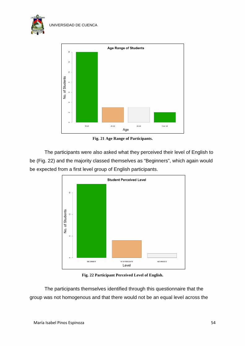
María Isabel Pinos Espinoza 54
UNIVERSIDAD DE CUENCA
Fig. 21 Age Range of Participants.
The participants were also asked what they perceived their level of English to
be (Fig. 22) and the majority classed themselves as “Beginners”, which again would
be expected from a first level group of English participants.
Fig. 22 Participant Perceived Level of English.
The participants themselves identified through this questionnaire that the
group was not homogenous and that there would not be an equal level across the
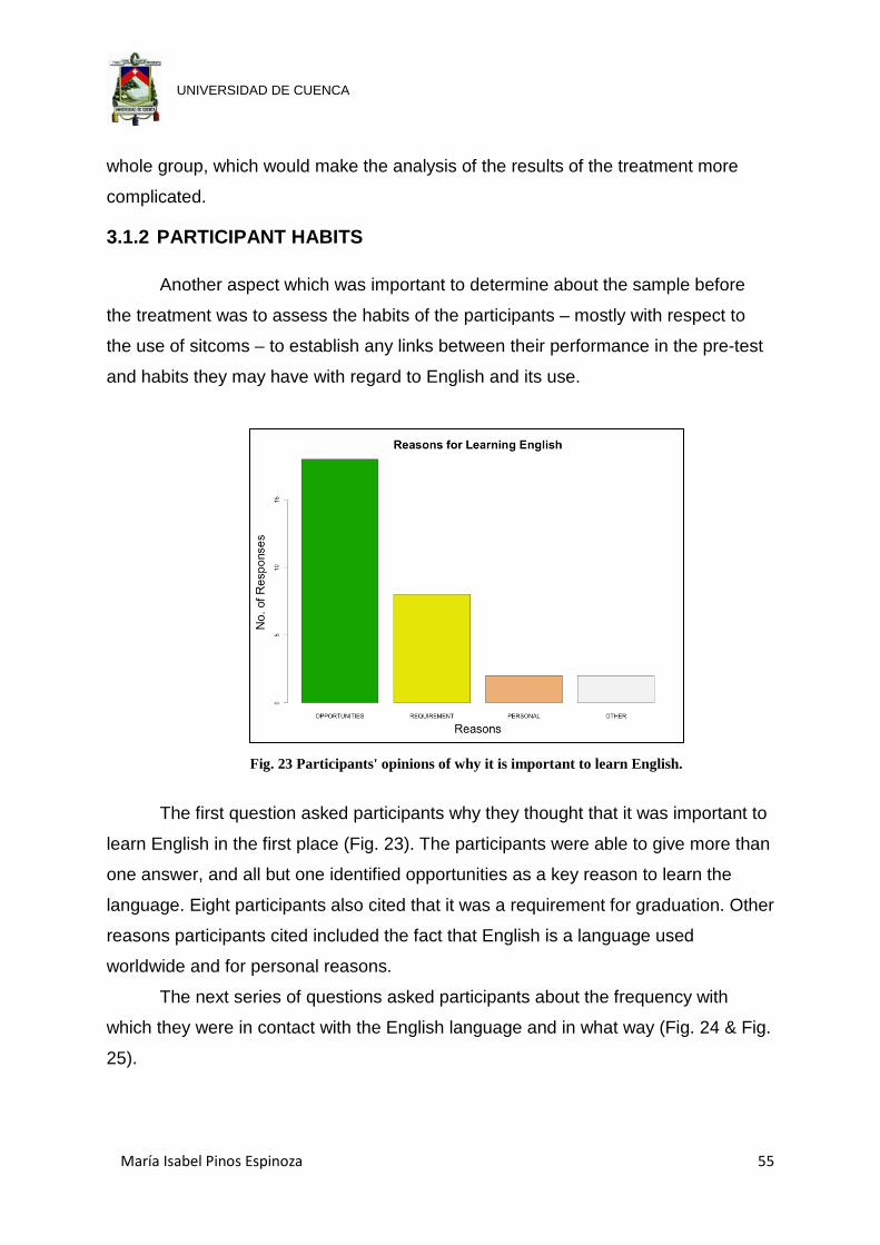
María Isabel Pinos Espinoza 55
UNIVERSIDAD DE CUENCA
whole group, which would make the analysis of the results of the treatment more
complicated.
3.1.2 PARTICIPANT HABITS
Another aspect which was important to determine about the sample before
the treatment was to assess the habits of the participants – mostly with respect to
the use of sitcoms – to establish any links between their performance in the pre-test
and habits they may have with regard to English and its use.
Fig. 23 Participants' opinions of why it is important to learn English.
The first question asked participants why they thought that it was important to
learn English in the first place (Fig. 23). The participants were able to give more than
one answer, and all but one identified opportunities as a key reason to learn the
language. Eight participants also cited that it was a requirement for graduation. Other
reasons participants cited included the fact that English is a language used
worldwide and for personal reasons.
The next series of questions asked participants about the frequency with
which they were in contact with the English language and in what way (Fig. 24 & Fig.
25).
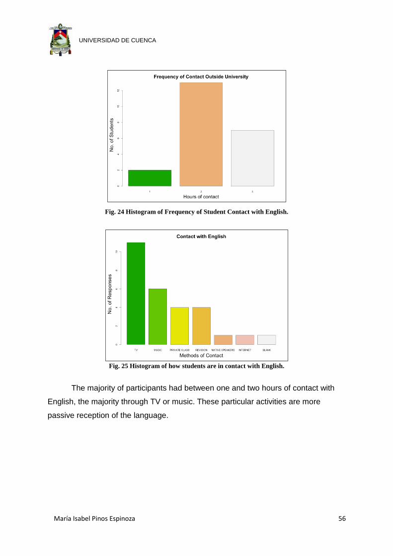
María Isabel Pinos Espinoza 56
UNIVERSIDAD DE CUENCA
Fig. 24 Histogram of Frequency of Student Contact with English.
Fig. 25 Histogram of how students are in contact with English.
The majority of participants had between one and two hours of contact with
English, the majority through TV or music. These particular activities are more
passive reception of the language.
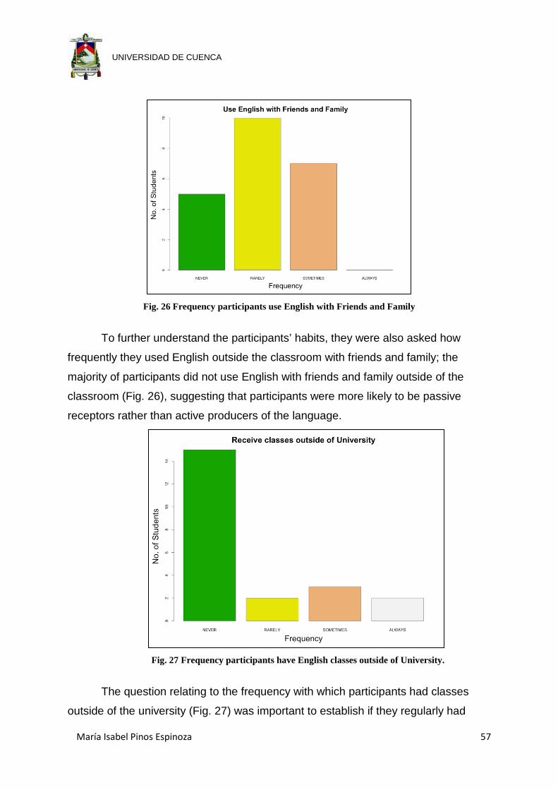
María Isabel Pinos Espinoza 57
UNIVERSIDAD DE CUENCA
Fig. 26 Frequency participants use English with Friends and Family
To further understand the participants’ habits, they were also asked how
frequently they used English outside the classroom with friends and family; the
majority of participants did not use English with friends and family outside of the
classroom (Fig. 26), suggesting that participants were more likely to be passive
receptors rather than active producers of the language.
Fig. 27 Frequency participants have English classes outside of University.
The question relating to the frequency with which participants had classes
outside of the university (Fig. 27) was important to establish if they regularly had
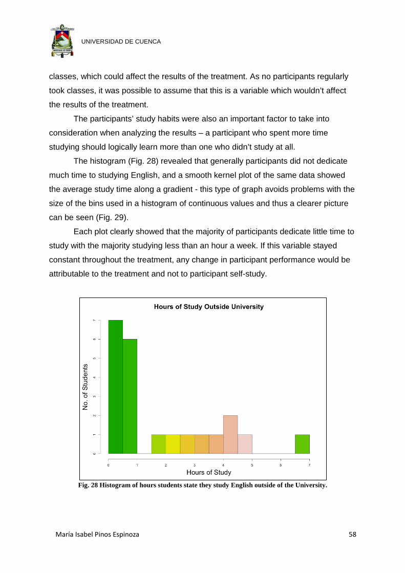
María Isabel Pinos Espinoza 58
UNIVERSIDAD DE CUENCA
classes, which could affect the results of the treatment. As no participants regularly
took classes, it was possible to assume that this is a variable which wouldn’t affect
the results of the treatment.
The participants’ study habits were also an important factor to take into
consideration when analyzing the results – a participant who spent more time
studying should logically learn more than one who didn’t study at all.
The histogram (Fig. 28) revealed that generally participants did not dedicate
much time to studying English, and a smooth kernel plot of the same data showed
the average study time along a gradient - this type of graph avoids problems with the
size of the bins used in a histogram of continuous values and thus a clearer picture
can be seen (Fig. 29).
Each plot clearly showed that the majority of participants dedicate little time to
study with the majority studying less than an hour a week. If this variable stayed
constant throughout the treatment, any change in participant performance would be
attributable to the treatment and not to participant self-study.
Fig. 28 Histogram of hours students state they study English outside of the University.
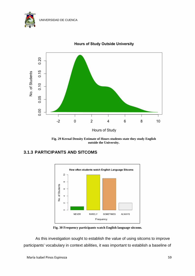
María Isabel Pinos Espinoza 59
UNIVERSIDAD DE CUENCA
Fig. 29 Kernal Density Estimate of Hours students state they study English
outside the University.
3.1.3 PARTICIPANTS AND SITCOMS
Fig. 30 Frequency participants watch English language sitcoms.
As this investigation sought to establish the value of using sitcoms to improve
participants’ vocabulary in context abilities, it was important to establish a baseline of
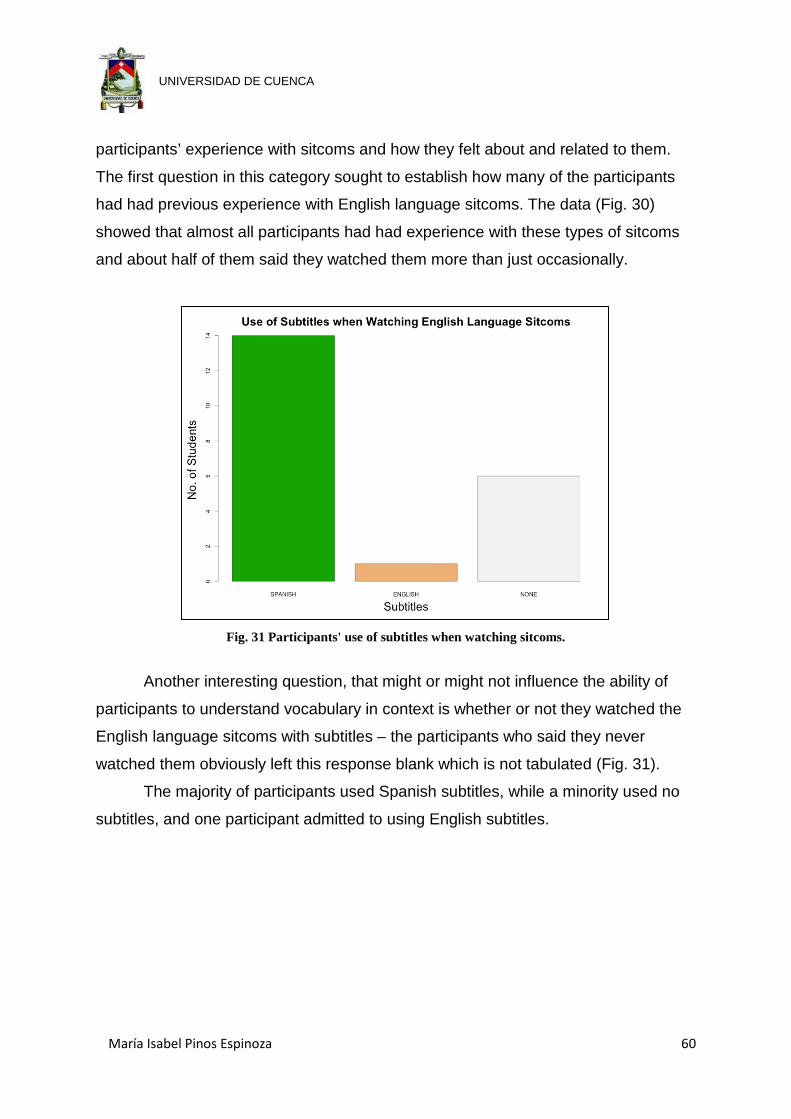
María Isabel Pinos Espinoza 60
UNIVERSIDAD DE CUENCA
participants’ experience with sitcoms and how they felt about and related to them.
The first question in this category sought to establish how many of the participants
had had previous experience with English language sitcoms. The data (Fig. 30)
showed that almost all participants had had experience with these types of sitcoms
and about half of them said they watched them more than just occasionally.
Fig. 31 Participants' use of subtitles when watching sitcoms.
Another interesting question, that might or might not influence the ability of
participants to understand vocabulary in context is whether or not they watched the
English language sitcoms with subtitles – the participants who said they never
watched them obviously left this response blank which is not tabulated (Fig. 31).
The majority of participants used Spanish subtitles, while a minority used no
subtitles, and one participant admitted to using English subtitles.

María Isabel Pinos Espinoza 61
UNIVERSIDAD DE CUENCA
Fig. 32 Number of hours participants had spent watching sitcoms the previous week.
When asked how many times the participants watched sitcoms the previous
week, the majority claimed to have watched between one and two hours of sitcoms
(Fig. 32). This tied in with the response to the question with what frequency
participants watch sitcoms. This suggests that participants were aware of how much
TV they watch.
Fig. 33 Relationship between stated frequency of viewing sitcoms and
number of hours spent watching sitcoms the previous week
A significant relationship was found between the amount of sitcoms the
participants watched the previous week and the frequency that participants claimed
to watch sitcoms in general (Pearson's Chi-squared test (X2 = 21.55, df = 6, p-value
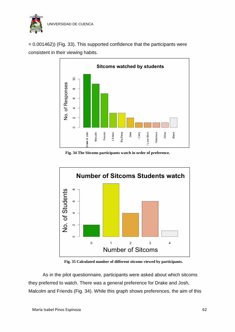
María Isabel Pinos Espinoza 62
UNIVERSIDAD DE CUENCA
= 0.001462)) (Fig. 33). This supported confidence that the participants were
consistent in their viewing habits.
Fig. 34 The Sitcoms participants watch in order of preference.
Fig. 35 Calculated number of different sitcoms viewed by participants.
As in the pilot questionnaire, participants were asked about which sitcoms
they preferred to watch. There was a general preference for Drake and Josh,
Malcolm and Friends (Fig. 34). While this graph shows preferences, the aim of this

María Isabel Pinos Espinoza 63
UNIVERSIDAD DE CUENCA
question was also to gauge the number of sitcoms that participants watched. The
results are shown in Fig. 35.
Fig. 36 Reasons participants gave for watching sitcoms.
The last part of the questionnaire asked participants about their opinions and
thoughts about sitcoms. The first question asked participants the reason why they
watched sitcoms in the first place. Participants could give multiple responses to this
question and almost all of them stated that it was because they were fun to watch
and a large minority stated that they watched them to learn English and some
included the reason that sitcoms contained real language (Fig. 36).
The last two questions asked participants how they considered that the use of
sitcoms had helped them learn English, the first on a personal level and the second
question in a group environment. The overwhelming response to both questions was
pronunciation and vocabulary although pronunciation was greater on a personal
level, and vocabulary in a group setting.
The data of these two questions were compared statistically using Pearson's
Chi-squared test, and the results show that there was no significant difference
between the two answers (X2 = 78.83, df = 24, p-value = 9.324e-08), despite some
participants adding grammar as something they learned in a group setting (Fig. 37
and Fig. 38).

María Isabel Pinos Espinoza 64
UNIVERSIDAD DE CUENCA
3.2. PRE-TEST ANALYSIS
The pre-test was one of the most important instruments in this investigation as
it not only identified the participants’ level prior to the treatment, but also permitted
investigation into which habits or previous experience may affect participant’s
abilities in the various aspects of English encountered in the test. As the test was
made up of three distinct aspects of vocabulary learning and testing, the results were
analysed on four levels: Vocabulary: Raw knowledge of words; Vocabulary in
Context: Using context clues to help understand the meaning of words; Reading:
Finding the correct word to match the meaning given; and finally the overall grade for
the test was also analysed.
3.2.1 OVERALL PRE-TEST RESULTS
The histogram of participants’ scores showed very skewed scores. Rather
than the bell-shaped curve that would be expected when graphing test scores, there
were two distinct peaks and one datum much further away (Fig. 39). The highest
possible score was twenty-seven, and only one participant came close to the
maximum score while four others managed to score over 50%.
Fig. 37 How participants believe sitcoms have helped them in their English learning.
Fig. 38 How participants feel the watching of sitcoms in a group environment has helped them learn.
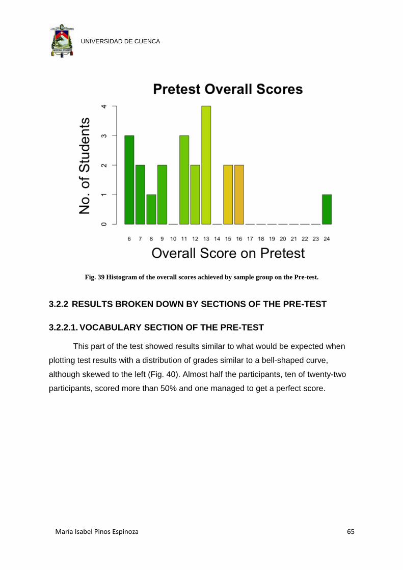
María Isabel Pinos Espinoza 65
UNIVERSIDAD DE CUENCA
Fig. 39 Histogram of the overall scores achieved by sample group on the Pre-test.
3.2.2 RESULTS BROKEN DOWN BY SECTIONS OF THE PRE-TEST
3.2.2.1. VOCABULARY SECTION OF THE PRE-TEST
This part of the test showed results similar to what would be expected when
plotting test results with a distribution of grades similar to a bell-shaped curve,
although skewed to the left (Fig. 40). Almost half the participants, ten of twenty-two
participants, scored more than 50% and one managed to get a perfect score.

María Isabel Pinos Espinoza 66
UNIVERSIDAD DE CUENCA
Fig. 40 Histogram of scores on the vocabulary section of the Pre-test.
3.2.2.2. VOCABULARY IN CONTEXT SECTION OF THE PRE-TEST
The results of this section also had a good approximation to a bell-curve albeit
with a long tail (Fig. 41). The data from this section showed that the whole group
appeared to be normally distributed with respect to this ability. Although there was a
very good curve, it was toward the lower score range; this section had a possible ten
points and the majority of participants got less than 50% right in this section – only
two participants managed to score higher.

María Isabel Pinos Espinoza 67
UNIVERSIDAD DE CUENCA
Fig. 41 Histogram of scores on the vocabulary in context section of the Pre-test.
3.2.2.3. READING SECTION OF PRE-TEST
The data from this section also showed a good approximation to a bell curve,
although as above, it was skewed toward the lower end of the possible scores with 7
being the highest score possible (Fig. 42). Seven participants managed to score
higher than 50%.
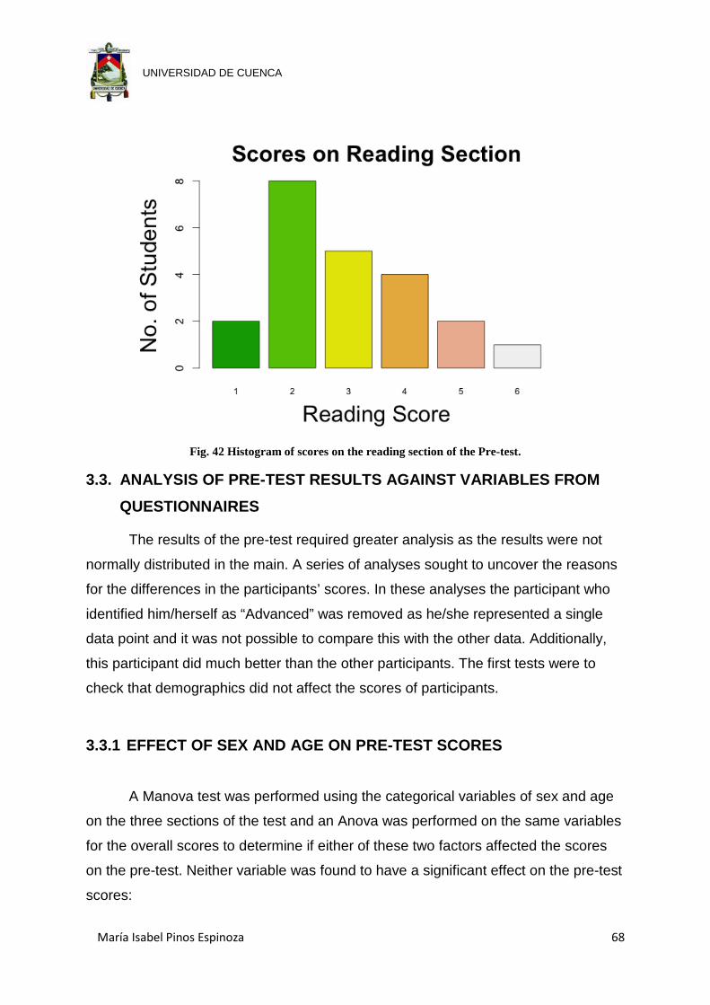
María Isabel Pinos Espinoza 68
UNIVERSIDAD DE CUENCA
Fig. 42 Histogram of scores on the reading section of the Pre-test.
3.3. ANALYSIS OF PRE-TEST RESULTS AGAINST VARIABLES FROM
QUESTIONNAIRES
The results of the pre-test required greater analysis as the results were not
normally distributed in the main. A series of analyses sought to uncover the reasons
for the differences in the participants’ scores. In these analyses the participant who
identified him/herself as “Advanced” was removed as he/she represented a single
data point and it was not possible to compare this with the other data. Additionally,
this participant did much better than the other participants. The first tests were to
check that demographics did not affect the scores of participants.
3.3.1 EFFECT OF SEX AND AGE ON PRE-TEST SCORES
A Manova test was performed using the categorical variables of sex and age
on the three sections of the test and an Anova was performed on the same variables
for the overall scores to determine if either of these two factors affected the scores
on the pre-test. Neither variable was found to have a significant effect on the pre-test
scores:

María Isabel Pinos Espinoza 69
UNIVERSIDAD DE CUENCA
Manova for Age Df Pillai approx F num Df den Df Pr(>F)
age 3 0.215 0.439 9 51 0.91
Residuals 17
Manova for Gender Df Pillai approx F num Df den Df Pr(>F)
sex 1 0.181 1.25 3 17 0.32
Residuals 19
Anova for Age Df Sum Sq Mean Sq F value Pr(>F)
age 3 10.78 3.595 0.287 0.834
Residuals 17 213.03 12.531
Anova for Gender Df Sum Sq Mean Sq F value Pr(>F)
age 3 10.78 3.595 0.287 0.834
Residuals 17 213.03 12.531
These data suggested that as there was no significant difference in the results
based on these two variables the whole group should be treated as one.
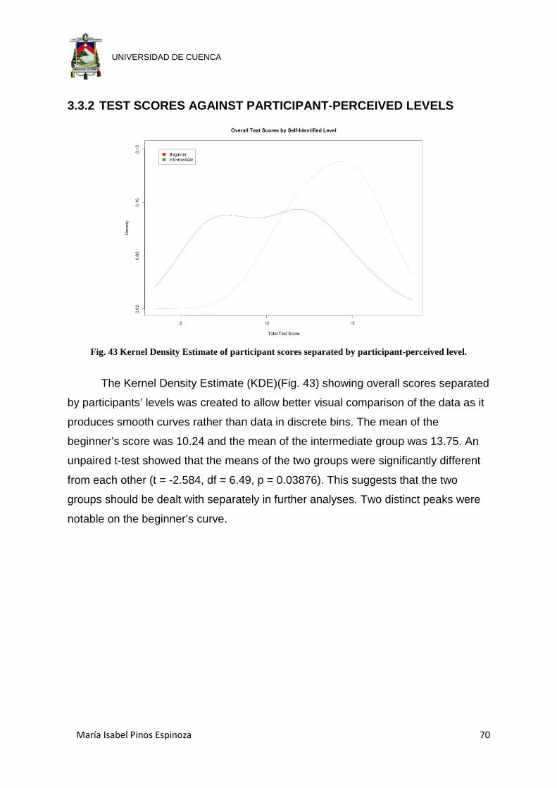
María Isabel Pinos Espinoza 70
UNIVERSIDAD DE CUENCA
3.3.2 TEST SCORES AGAINST PARTICIPANT-PERCEIVED LEVELS
Fig. 43 Kernel Density Estimate of participant scores separated by participant-perceived level.
The Kernel Density Estimate (KDE)(Fig. 43) showing overall scores separated
by participants’ levels was created to allow better visual comparison of the data as it
produces smooth curves rather than data in discrete bins. The mean of the
beginner’s score was 10.24 and the mean of the intermediate group was 13.75. An
unpaired t-test showed that the means of the two groups were significantly different
from each other (t = -2.584, df = 6.49, p = 0.03876). This suggests that the two
groups should be dealt with separately in further analyses. Two distinct peaks were
notable on the beginner’s curve.

María Isabel Pinos Espinoza 71
UNIVERSIDAD DE CUENCA
Fig. 44 Kernel Density Estimate of vocabulary scores separated by participant-perceived level.
Fig. 44, the KDE of vocabulary score by self-identified level, showed a similar
pattern to the overall scores, and again two distinct peaks were notable, although
this time in the Intermediate results. The means of the vocabulary scores of two
groups were: Beginners = 4.35 and Intermediates = 7.50. An unpaired t-test
confirmed what could be seen visually that there was a significant difference
between the means of the two groups (t = -3.22, df = 4.801, p = 0.02487). This again
suggests that the two groups should be treated separately in further analyses.

María Isabel Pinos Espinoza 72
UNIVERSIDAD DE CUENCA
Fig. 45 Kernal Density Estimate of vocabulary in context scores
separated by participant-perceived level.
The means of the two groups in the vocabulary in context section of the test
were very similar (Beginners = 3, Intermediates = 3.75) (Fig. 45) and an unpaired t-
test confirmed that there was no significant difference between the two means (t = -
1.247, df = 7.026, p = 0.2522). This result would suggest that the two groups should
be analysed together.
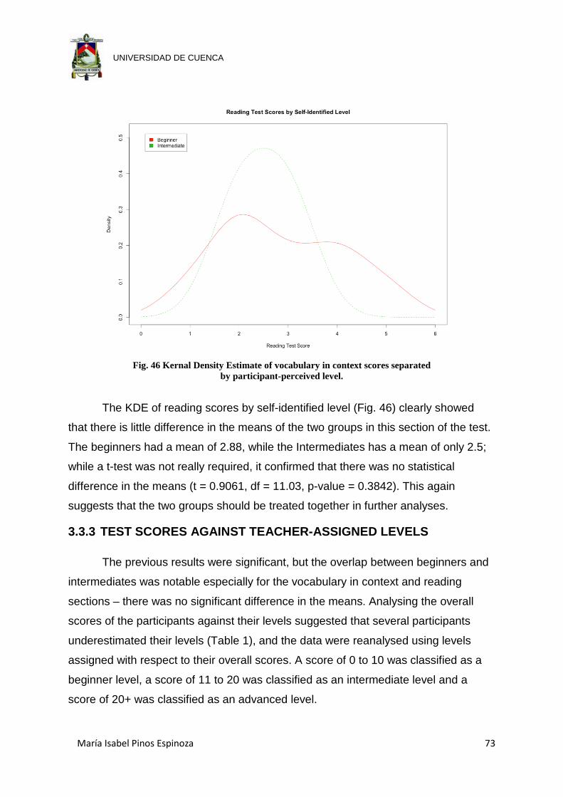
María Isabel Pinos Espinoza 73
UNIVERSIDAD DE CUENCA
Fig. 46 Kernal Density Estimate of vocabulary in context scores separated
by participant-perceived level.
The KDE of reading scores by self-identified level (Fig. 46) clearly showed
that there is little difference in the means of the two groups in this section of the test.
The beginners had a mean of 2.88, while the Intermediates has a mean of only 2.5;
while a t-test was not really required, it confirmed that there was no statistical
difference in the means (t = 0.9061, df = 11.03, p-value = 0.3842). This again
suggests that the two groups should be treated together in further analyses.
3.3.3 TEST SCORES AGAINST TEACHER-ASSIGNED LEVELS
The previous results were significant, but the overlap between beginners and
intermediates was notable especially for the vocabulary in context and reading
sections – there was no significant difference in the means. Analysing the overall
scores of the participants against their levels suggested that several participants
underestimated their levels (Table 1), and the data were reanalysed using levels
assigned with respect to their overall scores. A score of 0 to 10 was classified as a
beginner level, a score of 11 to 20 was classified as an intermediate level and a
score of 20+ was classified as an advanced level.

María Isabel Pinos Espinoza 74
UNIVERSIDAD DE CUENCA
Table showing Changes to levels assigned by the Researcher
PARTICIPANT Participant-
identified level
Overall Pre-test
Score
Teacher-assigned
Level
Participant 1 ADVANCED 24 ADVANCED
Participant 2 INTERMEDIATE 16 INTERMEDIATE
Participant 3 BEGINNER 16 INTERMEDIATE
Participant 4 BEGINNER 15 INTERMEDIATE
Participant 5 INTERMEDIATE 15 INTERMEDIATE
Participant 6 BEGINNER 13 INTERMEDIATE
Participant 7 BEGINNER 13 INTERMEDIATE
Participant 8 INTERMEDIATE 13 INTERMEDIATE
Participant 9 BEGINNER 13 INTERMEDIATE
Participant 10 BEGINNER 12 INTERMEDIATE
Participant 11 BEGINNER 12 INTERMEDIATE
Participant 12 BEGINNER 11 INTERMEDIATE
Participant 13 INTERMEDIATE 11 INTERMEDIATE
Participant 14 BEGINNER 11 INTERMEDIATE
Participant 15 BEGINNER 9 BEGINNER
Participant 16 BEGINNER 9 BEGINNER
Participant 17 BEGINNER 8 BEGINNER
Participant 18 BEGINNER 7 BEGINNER
Participant 19 BEGINNER 7 BEGINNER
Participant 20 BEGINNER 6 BEGINNER
Participant 21 BEGINNER 6 BEGINNER
Participant 22 BEGINNER 6 BEGINNER Table 1 Changes made to participant levels using overall Pre-test score as a measure.
This would obviously affect the means of the overall score for beginners and
intermediates as they have been artificially separated, but of greater interest is the
effect it may have on the distinct sections of the test.

María Isabel Pinos Espinoza 75
UNIVERSIDAD DE CUENCA
Fig. 47 Kernel Density Estimate of Overall test scores separated by Teacher-assigned Levels.
The graph of overall test scores by teacher-assigned level unsurprisingly had
a greater separation between the two means (Beginners = 7.25, Intermediates =
13.15) (Fig. 47), and the differences were highly significant when the unpaired t-test
was applied (t = -8.707, df = 18.51, p = 5.744e-08) - the p value is much lower than
the original (p = 0.03876).
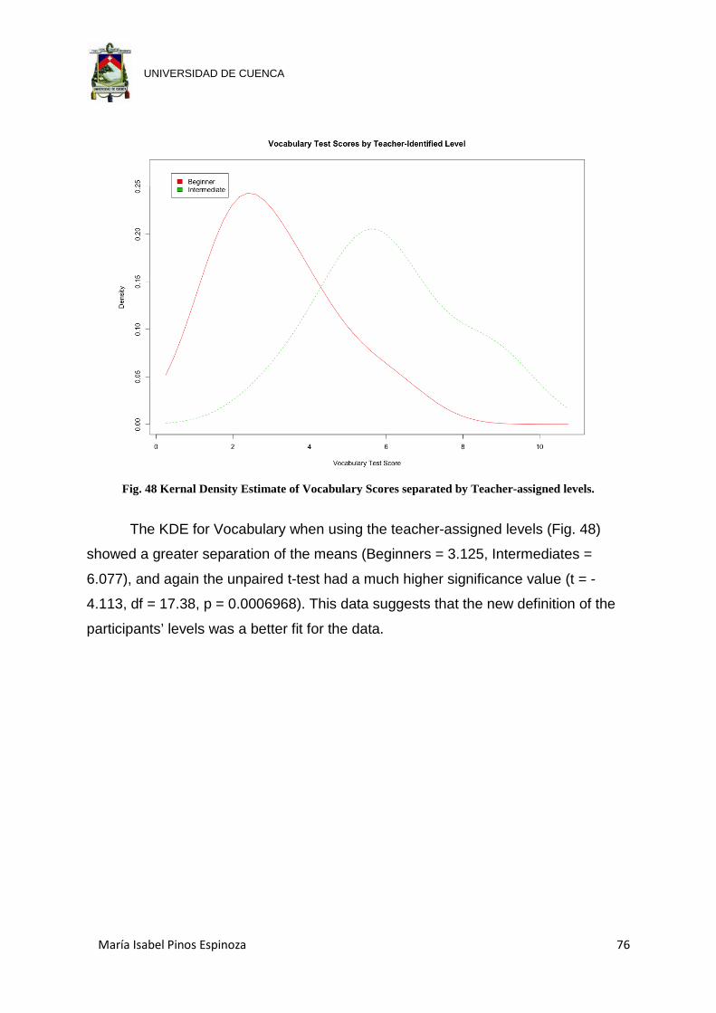
María Isabel Pinos Espinoza 76
UNIVERSIDAD DE CUENCA
Fig. 48 Kernal Density Estimate of Vocabulary Scores separated by Teacher-assigned levels.
The KDE for Vocabulary when using the teacher-assigned levels (Fig. 48)
showed a greater separation of the means (Beginners = 3.125, Intermediates =
6.077), and again the unpaired t-test had a much higher significance value (t = -
4.113, df = 17.38, p = 0.0006968). This data suggests that the new definition of the
participants’ levels was a better fit for the data.
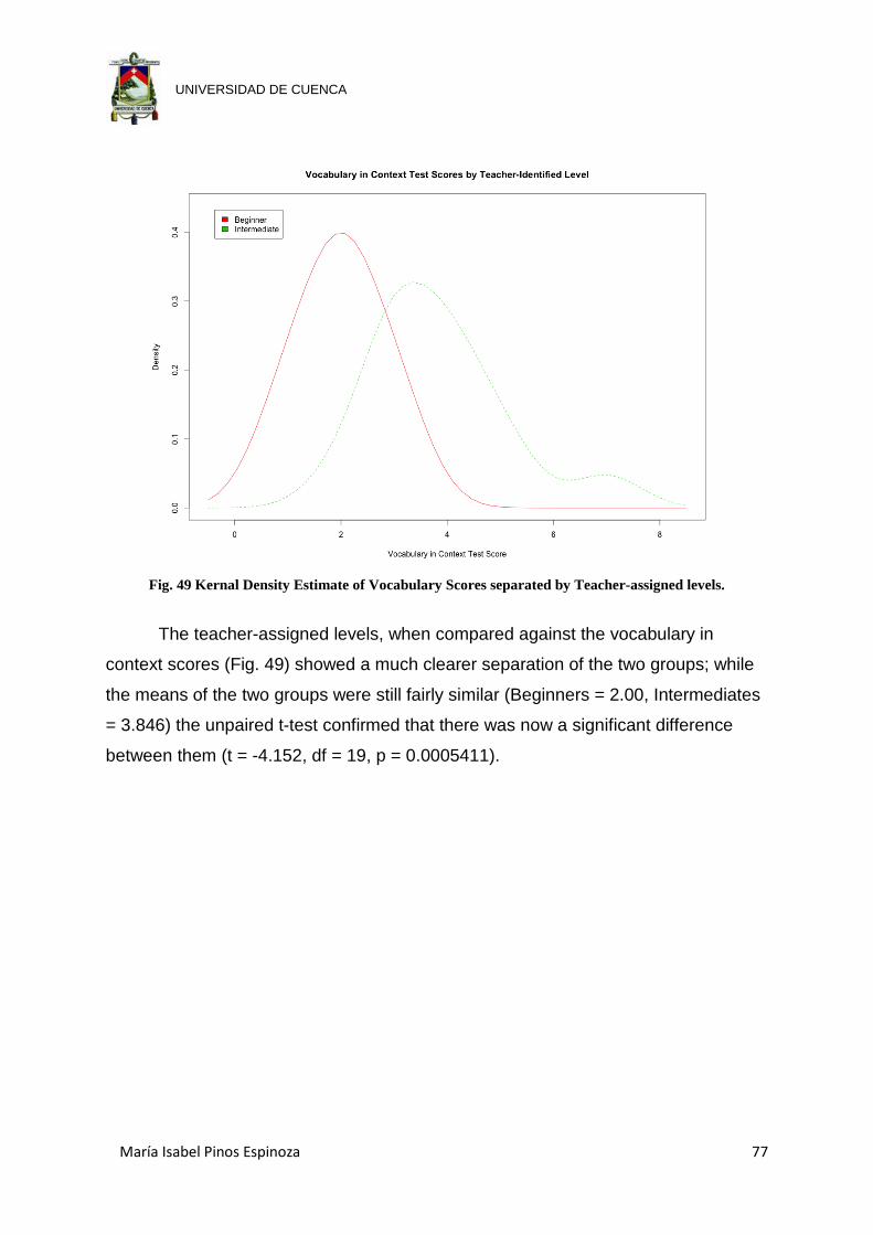
María Isabel Pinos Espinoza 77
UNIVERSIDAD DE CUENCA
Fig. 49 Kernal Density Estimate of Vocabulary Scores separated by Teacher-assigned levels.
The teacher-assigned levels, when compared against the vocabulary in
context scores (Fig. 49) showed a much clearer separation of the two groups; while
the means of the two groups were still fairly similar (Beginners = 2.00, Intermediates
= 3.846) the unpaired t-test confirmed that there was now a significant difference
between them (t = -4.152, df = 19, p = 0.0005411).
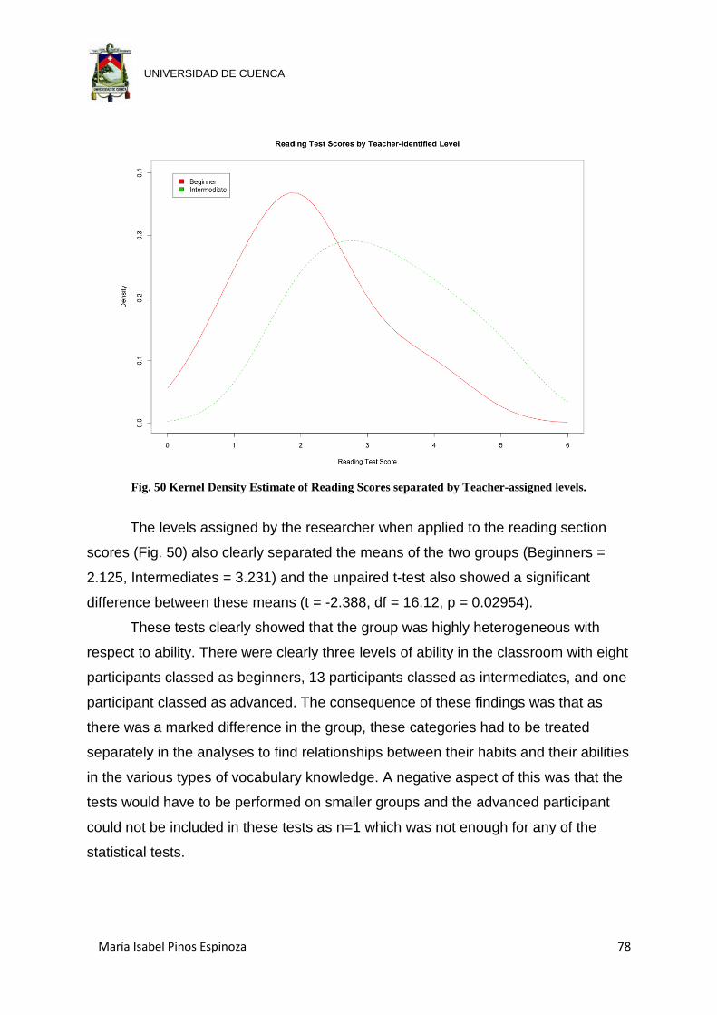
María Isabel Pinos Espinoza 78
UNIVERSIDAD DE CUENCA
Fig. 50 Kernel Density Estimate of Reading Scores separated by Teacher-assigned levels.
The levels assigned by the researcher when applied to the reading section
scores (Fig. 50) also clearly separated the means of the two groups (Beginners =
2.125, Intermediates = 3.231) and the unpaired t-test also showed a significant
difference between these means (t = -2.388, df = 16.12, p = 0.02954).
These tests clearly showed that the group was highly heterogeneous with
respect to ability. There were clearly three levels of ability in the classroom with eight
participants classed as beginners, 13 participants classed as intermediates, and one
participant classed as advanced. The consequence of these findings was that as
there was a marked difference in the group, these categories had to be treated
separately in the analyses to find relationships between their habits and their abilities
in the various types of vocabulary knowledge. A negative aspect of this was that the
tests would have to be performed on smaller groups and the advanced participant
could not be included in these tests as n=1 which was not enough for any of the
statistical tests.

María Isabel Pinos Espinoza 79
UNIVERSIDAD DE CUENCA
3.3.4 MANOVA AND ANOVA TESTS MANOVA tests were chosen to analyse the data as it is a Multivariate
Analysis of Variance that allowed us to test multiple dependent variables, in this case
the results of the three sections of the Pre-test, against multiple independent
variables, which were the responses to the questionnaire. By using MANOVA, it was
possible to go beyond looking at the effect of one independent variable and look for
patterns or interactions between independent variables (Scheiner, 99-102). A simple
calculation within the statistics program (RStudio, Version 0.98.501) illustrates the
ANOVA responses of each individual variable. Significance was measured at 95%.
3.3.4.1. EFFECTS OF BEGINNER LEVEL PARTICIPANT HABITS ON PRE-TEST SCORES
Due to the small number of participants within this group (n=8), no more than
two independent variables could be used at the same time to test for correlations
between habits.
At first sight, the results looked very promising with several of the MANOVAs
showing significant effects (Appendix 7). However, on closer inspection of the
results, it was found that one of the data points was seriously skewing the results.
The participant in question got one of the higher scores in the vocabulary section, yet
claimed to never watch sitcoms. This result was causing many of the ANOVAs of
individual parts of the test – particularly the vocabulary section – to show significant
links when there were none obvious to see.
As a result of this – given that one of the aims of this analysis was to seek
patterns of habits that may influence participant ability in vocabulary – this participant
was removed from the matrix and the tests were rerun (Appendix 8). The results of
the new set of tests were much less significant and only one slightly significant
correlation was found related with how often the participants had watched sitcoms
the previous week.

María Isabel Pinos Espinoza 80
UNIVERSIDAD DE CUENCA
Response PRT3 :
Df Sum Sq Mean Sq F value Pr(>F)
howoften 2 5.36 2.679 7.14 0.048 *
Residuals 4 1.50 0.375
---
Signif. codes: 0 '***' 0.001 '**' 0.01 '*' 0.05 '.' 0.1 ' ' 1
Fig. 51 Boxplot showing the results of Reading score against Frequency
participants watched Sitcoms the previous week.
As the graph in Fig. 51 showed, there was a clear distinction between the
frequency participants watch sitcoms and their score on reading; however, the
distinction did not take into account the fact that participants who did not watch any
sitcoms at all did better than those who watched 1-2 hours of sitcoms. A logical
reading of this graph was that although statistically it was significant, it essentially
meant little.

María Isabel Pinos Espinoza 81
UNIVERSIDAD DE CUENCA
3.3.4.2. EFFECTS OF INTERMEDIATE LEVEL PARTICIPANT HABITS ON PRE-TEST SCORES
The same tests were performed on the intermediate participants. In this case,
no significant effect of habits was found for the results of the pre-test (Appendix 9).
An intermediate participant also claimed to never watch sitcoms and so to be fair, the
tests were also run with the participant who never watched sitcoms removed from
the sample (Appendix 10), but again no significant correlations were found.
3.3.4.3. EFFECTS OF PARTICIPANT HABITS AT ALL LEVELS ON PRE-TEST SCORES
As no significant effects were found for level of participants, the data were
pooled and the tests were rerun (Appendix 11). The first set of tests included all
participants except the advanced participant. A fairly significant relationship was
found between their vocabulary in context score and the frequency with which
participants watched sitcoms combined with the number of sitcoms they watched:
Response PRT2 :
Df Sum Sq Mean Sq F value Pr(>F)
watch:No.Sitcoms 10 33.8 3.38 5.01 0.0089 **
Residuals 10 6.8 0.68
---
Signif. codes: 0 '***' 0.001 '**' 0.01 '*' 0.05 '.' 0.1 ' ' 1

María Isabel Pinos Espinoza 82
UNIVERSIDAD DE CUENCA
Fig. 52 Boxplot showing the scores on the Vocabulary in Context section of the pre-test against Frequency
with which participants watch sitcoms combined with the number of Sitcoms they watch.
As can be seen by the plot (Fig. 52), as with the response of beginners
reading scores to the frequency with which they watch sitcoms (Fig. 51), it was
difficult to understand the significant relationship until the boxplot was read looking at
the first combined variable separately; once done it was possible to see that there
was a trend towards improving grades relative to the number of sitcoms a participant
watched. A similar, yet slightly more significant, result was found for the frequency
with which participants watched sitcoms combined with the frequency with which
they used English outside of the classroom against their vocabulary in context score
(Fig. 53):

María Isabel Pinos Espinoza 83
UNIVERSIDAD DE CUENCA
Response PRT2 :
Df Sum Sq Mean Sq F value Pr(>F)
use:watch 8 31.1 3.88 4.91 0.0071 **
Residuals 12 9.5 0.79
---
Signif. codes: 0 '***' 0.001 '**' 0.01 '*' 0.05 '.' 0.1 ' ' 1
Fig. 53 Boxplot showing the scores on the Vocabulary in Context section of the pre-test against
Frequency with which participants watch sitcoms combined with the frequency with which they use English outside the classroom.
This plot had a better correlation, especially in the “sometimes watch sitcoms”
category, and a general trend towards higher ability with increased frequency of use
of English outside the classroom (note again the trends within the categories; those
who rarely watch sitcoms generally did better as they increase their use of English
outside of the classroom, as did those who sometimes watch sitcoms).
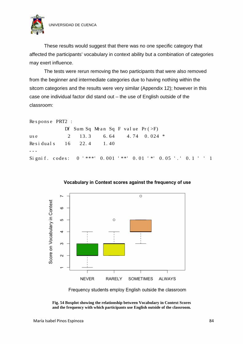
María Isabel Pinos Espinoza 84
UNIVERSIDAD DE CUENCA
These results would suggest that there was no one specific category that
affected the participants’ vocabulary in context ability but a combination of categories
may exert influence.
The tests were rerun removing the two participants that were also removed
from the beginner and intermediate categories due to having nothing within the
sitcom categories and the results were very similar (Appendix 12); however in this
case one individual factor did stand out – the use of English outside of the
classroom:
Response PRT2 :
Df Sum Sq Mean Sq F value Pr(>F)
use 2 13.3 6.64 4.74 0.024 *
Residuals 16 22.4 1.40
---
Signif. codes: 0 '***' 0.001 '**' 0.01 '*' 0.05 '.' 0.1 ' ' 1
Fig. 54 Boxplot showing the relationship between Vocabulary in Context Scores and the frequency with which participants use English outside of the classroom.

María Isabel Pinos Espinoza 85
UNIVERSIDAD DE CUENCA
Fig. 54 was the first to really show any kind of consistent relationship between
scores on the pre-test and habits. There was a clear positive relationship between
the frequency with which participants used English outside the classroom and their
scores in the vocabulary in context section of the pre-test. The results that were
significant in the previous tests with the whole group remained significant in this
round of tests; the relationship between their vocabulary in context score and the
frequency with which participants watched sitcoms combined with the number of
sitcoms they watched became more significant (p = 0.081), while for the frequency
with which participants watched sitcoms combined with the frequency with which
they used English outside of the classroom against their vocabulary in context score
the relationship became less significant (p = 0.015).
3.3.4.4. DISCUSSIONS AND CONCLUSIONS ABOUT THE RELATIONSHIPS BETWEEN PRE-TEST SCORES AND PARTICIPANT CHARACTERISTICS AND HABITS
There were essentially no relationships between participant habits and their
scores on the pre-test. The few relationships that could be considered as significant
relate to the use of the language outside the classroom, and a relationship between
the frequency participants watch sitcoms combined with either the use of the
language outside of the classroom or with the number of different sitcoms
participants watch.
Over all, there were not enough samples to truly explore the relationships
between the categories satisfactorily as to do these tests effectively several data
values have to fall into the majority of categories, and when data such as use of
English and frequency with watching sitcoms is combined, there were many blank
categories and several data points that had only one data value.
Analysing the results as they stand, it suggested that the need to use the
language (frequency of use outside the classroom) compelled participants to absorb
more vocabulary and use vocabulary in context tools to communicate. In other
words, this conditioning – added to the greater practice from watching more English
language sitcoms with greater frequency – improved participants’ abilities in this area
of language competence. By the same token, there was no discernible effect of
habits in the areas of raw vocabulary knowledge or reading vocabulary ability.

María Isabel Pinos Espinoza 86
UNIVERSIDAD DE CUENCA
3.4. EFFECT OF USING SITCOMS AS A TOOL FOR VOCABULARY LEARNING IN THE CLASSROOM
As the effects of participants’ habits on abilities in vocabulary tests were
minimal, it was possible to suggest that any effects seen on the post-test were
largely due to the treatment itself. The first set of statistical tests investigated if the
treatment had had any significant effect on the participants’ scores on the test in
general and on each of the distinct parts of the test. The groups identified by the
teacher as being beginners or intermediates were again used and the advanced
participant as a singleton was omitted as being impossible to compare.
3.4.1 COMPARISON OF FINAL RESULTS BETWEEN BEGINNERS AND INTERMEDIATES
The results of a series of unpaired t-tests showed that overall the participants
retained the differences between the groups with the means being significantly
different in all but the raw vocabulary section of the test suggesting a great
improvement in raw vocabulary by the beginner group (Table 2); however, of greater
interest in this study is how the groups had improved.
Mean
Beginners
Mean
Intermediates
t Df p-value
Overall 11.00 14.77 -3.851 13.33 0.0072
Vocabulary 5.75 6.54 -1.212 11.95 0.2488
Vocabulary
in Context
3.5 5.08 -2.469 18.13 0.0237
Reading 1.75 3.15 -3.171 13.33 0.0072 Table 2 Unpaired t-test results for posttest comparing beginners and intermediates.
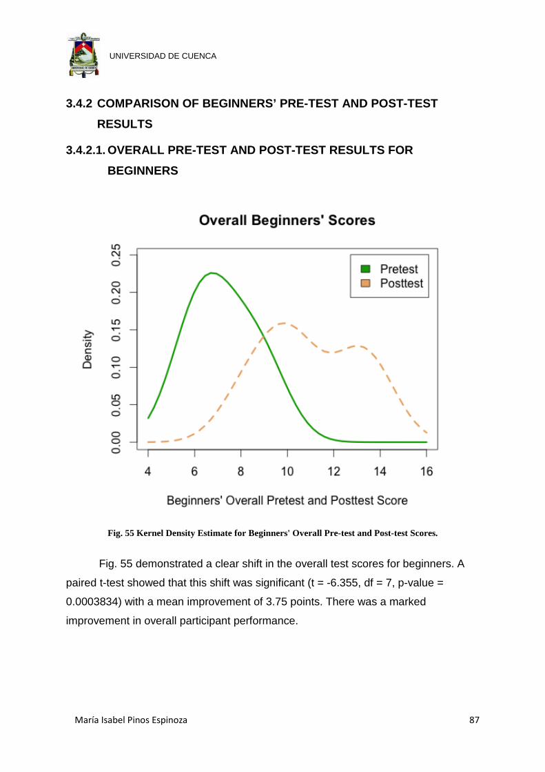
María Isabel Pinos Espinoza 87
UNIVERSIDAD DE CUENCA
3.4.2 COMPARISON OF BEGINNERS’ PRE-TEST AND POST-TEST RESULTS
3.4.2.1. OVERALL PRE-TEST AND POST-TEST RESULTS FOR BEGINNERS
Fig. 55 Kernel Density Estimate for Beginners' Overall Pre-test and Post-test Scores.
Fig. 55 demonstrated a clear shift in the overall test scores for beginners. A
paired t-test showed that this shift was significant (t = -6.355, df = 7, p-value =
0.0003834) with a mean improvement of 3.75 points. There was a marked
improvement in overall participant performance.
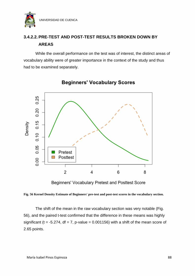
María Isabel Pinos Espinoza 88
UNIVERSIDAD DE CUENCA
3.4.2.2. PRE-TEST AND POST-TEST RESULTS BROKEN DOWN BY AREAS
While the overall performance on the test was of interest, the distinct areas of
vocabulary ability were of greater importance in the context of the study and thus
had to be examined separately.
Fig. 56 Kernel Density Estimate of Beginners' pre-test and post-test scores in the vocabulary section.
The shift of the mean in the raw vocabulary section was very notable (Fig.
56), and the paired t-test confirmed that the difference in these means was highly
significant (t = -5.274, df = 7, p-value = 0.001156) with a shift of the mean score of
2.65 points.
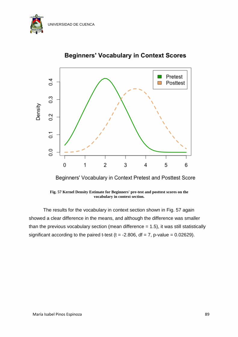
María Isabel Pinos Espinoza 89
UNIVERSIDAD DE CUENCA
Fig. 57 Kernel Density Estimate for Beginners' pre-test and posttest scores on the
vocabulary in context section.
The results for the vocabulary in context section shown in Fig. 57 again
showed a clear difference in the means, and although the difference was smaller
than the previous vocabulary section (mean difference = 1.5), it was still statistically
significant according to the paired t-test (t = -2.806, df = 7, p-value = 0.02629).

María Isabel Pinos Espinoza 90
UNIVERSIDAD DE CUENCA
Fig. 58 Kernel Density Estimate of Beginners' pre-test and post-test
scores on the reading section.
Fig. 58 clearly showed that there had been no improvement in the reading
section of the test by beginner participants (t = 1.158, df = 7, p-value = 0.2849) with
an actual lowering of mean performance with the mean score dropping 0.38 points.
These results showed that the treatment had a positive effect on participants’
abilities in raw vocabulary and vocabulary in context, while having no effect on their
reading abilities.
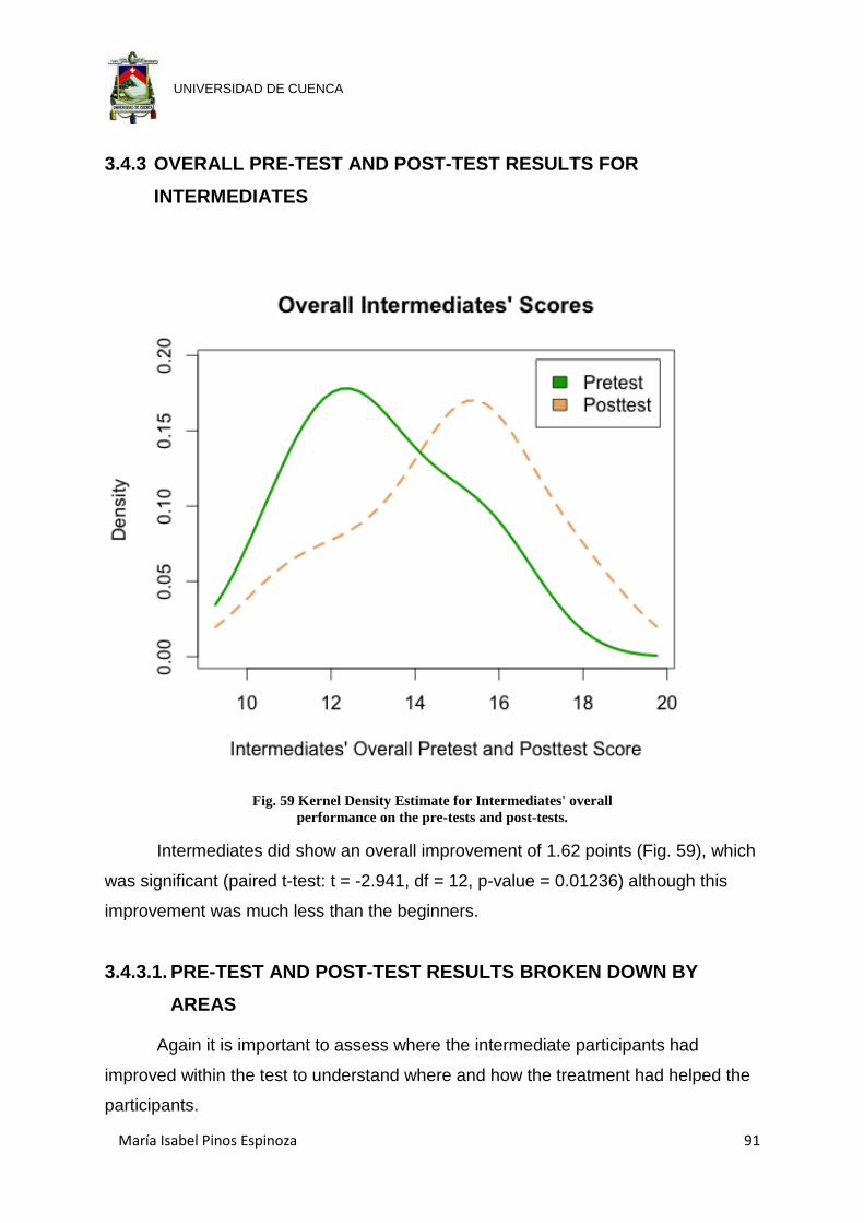
María Isabel Pinos Espinoza 91
UNIVERSIDAD DE CUENCA
3.4.3 OVERALL PRE-TEST AND POST-TEST RESULTS FOR INTERMEDIATES
Fig. 59 Kernel Density Estimate for Intermediates' overall
performance on the pre-tests and post-tests.
Intermediates did show an overall improvement of 1.62 points (Fig. 59), which
was significant (paired t-test: t = -2.941, df = 12, p-value = 0.01236) although this
improvement was much less than the beginners.
3.4.3.1. PRE-TEST AND POST-TEST RESULTS BROKEN DOWN BY AREAS
Again it is important to assess where the intermediate participants had
improved within the test to understand where and how the treatment had helped the
participants.
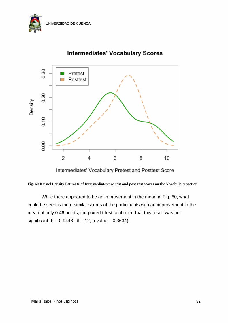
María Isabel Pinos Espinoza 92
UNIVERSIDAD DE CUENCA
Fig. 60 Kernel Density Estimate of Intermediates pre-test and post-test scores on the Vocabulary section.
While there appeared to be an improvement in the mean in Fig. 60, what
could be seen is more similar scores of the participants with an improvement in the
mean of only 0.46 points, the paired t-test confirmed that this result was not
significant (t = -0.9448, df = 12, p-value = 0.3634).

María Isabel Pinos Espinoza 93
UNIVERSIDAD DE CUENCA
Fig. 61 Kernel Density Estimate of intermediates pre-test and post-test
scores on the vocabulary in context section.
The curves shown in Fig. 61 showed very little change in the scores for the
majority of the participants although two participants who did exceptionally well (as
seen in the second hump of the Post-test) elevated the mean difference 1.23 points.
This difference was still not significantly different (t = -2.049, df = 12, p-value =
0.06303).

María Isabel Pinos Espinoza 94
UNIVERSIDAD DE CUENCA
Fig. 62 Kernel Density Estimate for Intermediates' pre-test
and posttest scores in the reading section.
Fig. 62 showed the results for the reading section and it was obvious that
there has been little change about the mean. In fact there had been an overall drop
in mean score by 0.08 points, although this was not significant (t = 0.21, df = 12, p-
value = 0.8372). The change in shape to the curve was due to more participants
getting 4 out of seven, but many participants actually did worse on the second test
and so the overall mean is the same.
These tests showed that while the intermediate participants did make
significant improvement to their overall score, it could not be attributed to any
particular section of the test.

María Isabel Pinos Espinoza 95
UNIVERSIDAD DE CUENCA
3.5. EFFECT OF TREATMENT ON THE TWO LEVELS
3.5.1 OVERALL IMPROVEMENT OF THE TWO LEVELS
The previous section showed that the treatment did not affect the two levels
equally, so an exploration of the differences between the improvements was merited.
Fig. 63 Boxplot showing the overall improvement of participants
separated by teacher-assigned level.
Fig. 63 clearly showed that the beginners improved their scores in general a
lot more than the intermediate participants (Mean beginners = 3.75, mean
intermediates = 1.62). An unpaired t-test confirmed that the difference was significant
(t = 2.648, df = 16.96, p-value = 0.01695).
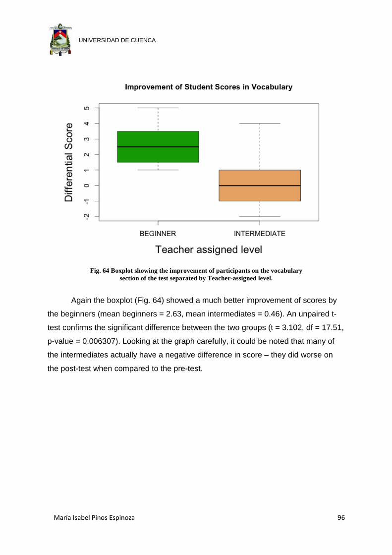
María Isabel Pinos Espinoza 96
UNIVERSIDAD DE CUENCA
Fig. 64 Boxplot showing the improvement of participants on the vocabulary
section of the test separated by Teacher-assigned level.
Again the boxplot (Fig. 64) showed a much better improvement of scores by
the beginners (mean beginners = 2.63, mean intermediates = 0.46). An unpaired t-
test confirms the significant difference between the two groups (t = 3.102, df = 17.51,
p-value = 0.006307). Looking at the graph carefully, it could be noted that many of
the intermediates actually have a negative difference in score – they did worse on
the post-test when compared to the pre-test.

María Isabel Pinos Espinoza 97
UNIVERSIDAD DE CUENCA
Fig. 65 Boxplot showing the difference in the pre-test and post-test scores on the vocabulary
in context section of the test separated by teacher-assigned level.
Fig. 65 showed mixed results; while there was generally a small improvement
of the beginner participants (mean = 1.5) the mean performance of the intermediate
group was lower (mean = 1.23). The circles on the graph are outliers, data points
that are far away from the mean, and in the intermediate group we can see that
some participants did improve substantially, although others did less well than in the
pre-test. A t-test confirmed that these results were not significantly different (t =
0.3348, df = 18.57, p-value = 0.7415).
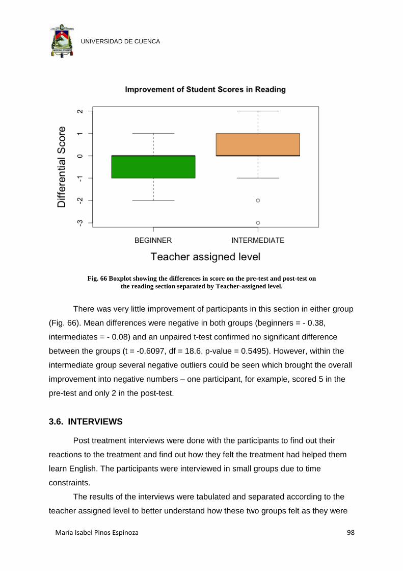
María Isabel Pinos Espinoza 98
UNIVERSIDAD DE CUENCA
Fig. 66 Boxplot showing the differences in score on the pre-test and post-test on
the reading section separated by Teacher-assigned level.
There was very little improvement of participants in this section in either group
(Fig. 66). Mean differences were negative in both groups (beginners = - 0.38,
intermediates = - 0.08) and an unpaired t-test confirmed no significant difference
between the groups (t = -0.6097, df = 18.6, p-value = 0.5495). However, within the
intermediate group several negative outliers could be seen which brought the overall
improvement into negative numbers – one participant, for example, scored 5 in the
pre-test and only 2 in the post-test.
3.6. INTERVIEWS
Post treatment interviews were done with the participants to find out their
reactions to the treatment and find out how they felt the treatment had helped them
learn English. The participants were interviewed in small groups due to time
constraints.
The results of the interviews were tabulated and separated according to the
teacher assigned level to better understand how these two groups felt as they were
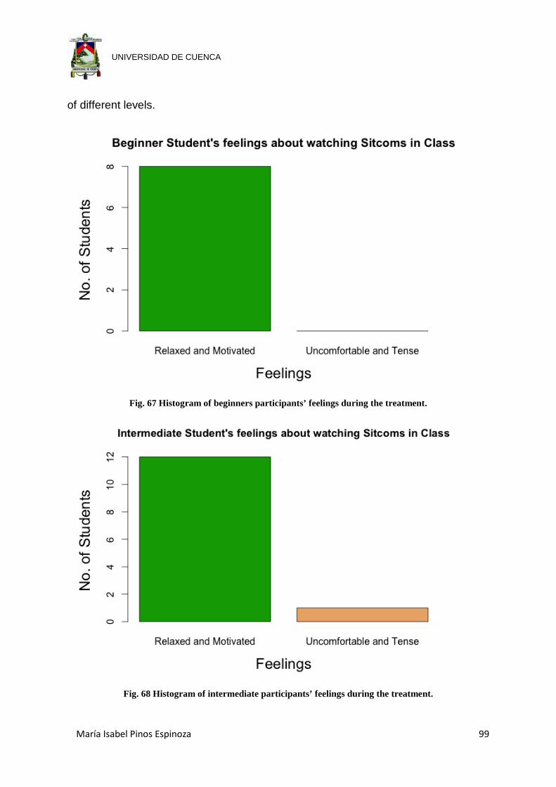
María Isabel Pinos Espinoza 99
UNIVERSIDAD DE CUENCA
of different levels.
Fig. 67 Histogram of beginners participants’ feelings during the treatment.
Fig. 68 Histogram of intermediate participants’ feelings during the treatment.

María Isabel Pinos Espinoza 100
UNIVERSIDAD DE CUENCA
Whether the treatment was successful or not, it was important to gauge how
the participants reacted during and after the treatment and in general the two levels
both felt comfortable during the treatment, although one participant did not (Fig. 67
and Fig. 68). As a classroom activity, the treatment was successful in the sense that
the participants did not have problems with the treatment itself, although as
previously noted the differing levels finished the set tasks at different times, which
must be addressed in future treatments.
Fig. 69 Histogram of intermediate participants’ feelings during the treatment.

María Isabel Pinos Espinoza 101
UNIVERSIDAD DE CUENCA
Fig. 70 Histogram of how difficult intermediate participants felt
understanding what they were watching.
The second question asked the participants how easy it had been to
understand what they were watching (Fig. 69 and Fig. 70). Here the levels
distinguished themselves in how they felt the watching of sitcoms only in English
was; all of the beginners felt this part of the treatment was difficult while only two of
the twelve intermediate participants thought that this part of the treatment was
difficult.
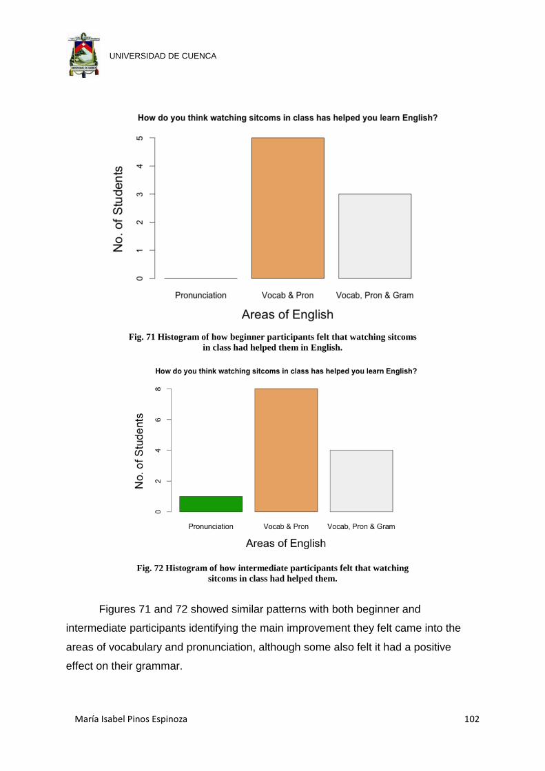
María Isabel Pinos Espinoza 102
UNIVERSIDAD DE CUENCA
Fig. 71 Histogram of how beginner participants felt that watching sitcoms
in class had helped them in English.
Fig. 72 Histogram of how intermediate participants felt that watching
sitcoms in class had helped them.
Figures 71 and 72 showed similar patterns with both beginner and
intermediate participants identifying the main improvement they felt came into the
areas of vocabulary and pronunciation, although some also felt it had a positive
effect on their grammar.
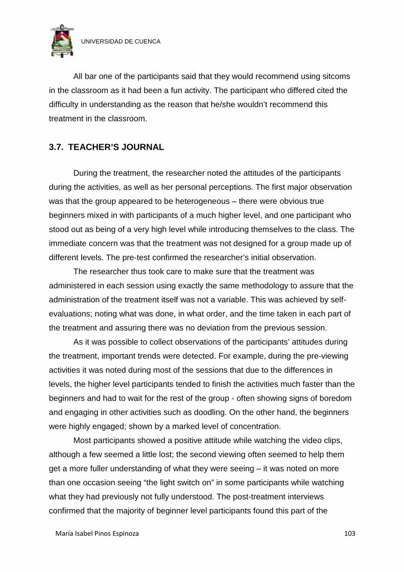
María Isabel Pinos Espinoza 103
UNIVERSIDAD DE CUENCA
All bar one of the participants said that they would recommend using sitcoms
in the classroom as it had been a fun activity. The participant who differed cited the
difficulty in understanding as the reason that he/she wouldn’t recommend this
treatment in the classroom.
3.7. TEACHER’S JOURNAL
During the treatment, the researcher noted the attitudes of the participants
during the activities, as well as her personal perceptions. The first major observation
was that the group appeared to be heterogeneous – there were obvious true
beginners mixed in with participants of a much higher level, and one participant who
stood out as being of a very high level while introducing themselves to the class. The
immediate concern was that the treatment was not designed for a group made up of
different levels. The pre-test confirmed the researcher’s initial observation.
The researcher thus took care to make sure that the treatment was
administered in each session using exactly the same methodology to assure that the
administration of the treatment itself was not a variable. This was achieved by self-
evaluations; noting what was done, in what order, and the time taken in each part of
the treatment and assuring there was no deviation from the previous session.
As it was possible to collect observations of the participants’ attitudes during
the treatment, important trends were detected. For example, during the pre-viewing
activities it was noted during most of the sessions that due to the differences in
levels, the higher level participants tended to finish the activities much faster than the
beginners and had to wait for the rest of the group - often showing signs of boredom
and engaging in other activities such as doodling. On the other hand, the beginners
were highly engaged; shown by a marked level of concentration.
Most participants showed a positive attitude while watching the video clips,
although a few seemed a little lost; the second viewing often seemed to help them
get a more fuller understanding of what they were seeing – it was noted on more
than one occasion seeing “the light switch on” in some participants while watching
what they had previously not fully understood. The post-treatment interviews
confirmed that the majority of beginner level participants found this part of the
María Isabel Pinos Espinoza 104
UNIVERSIDAD DE CUENCA
treatment difficult to understand, while the intermediate participants claimed to have
little problems understanding what they were watching. This phenomenon was noted
in the post-viewing activities as beginners were highly motivated to understand the
vocabulary that they had seen, and many questions were asked of the researcher
regarding the new vocabulary they were finding, while the higher level participants
did not seem to be as motivated to continue investigating the vocabulary. Exceptions
to the above included two intermediate participants who worked together extremely
well during the treatment, and responded the best during the post-test.
One of the things noted by the researcher was a general lax attitude to both
the pre-test and the post-test by the participants; their knowledge that the results had
no bearing on their final grades seemed to promote this attitude; In general the
researcher felt that the participants’ motivation during the pre- and post-viewing
activities was reflected in the improvements shown in the post-test.
While Mackey and Gass correctly stated that journals and diaries are usually
very subjective (203,204) – the researcher noted this style in her own notes – the
researcher found that it was extremely helpful in both assessing her teaching and
arriving at conclusions relating to the participants during this treatment. It would have
been unlikely that the researcher would have remembered which participants had
been the most engaged while analyzing the results after the treatment; as the
researcher made notes during each session, there was a record of participant
involvement as well as of the whole process.
The keeping of a journal during the treatment allowed the triangulation of the
data, thus pre-test, post-test, journal and interviews could all be used in conjunction
to reach conclusions.
María Isabel Pinos Espinoza 105
UNIVERSIDAD DE CUENCA
CHAPTER IV DISCUSSION, CONCLUSIONS AND RECOMMENDATIONS
4.1. LEVEL OF ENGLISH WITHIN THE SAMPLE GROUP
Participants were asked what they thought their level of English was
before they took the pre-test and the results were initially analysed based on
this. The results showed significant differences between the two means in
overall scores and in the vocabulary knowledge section although there were
unusual shapes in the Kernel Density Estimates. The overall scores of the
participants were analysed against their self-identified level and it was found
that many participants possibly underestimated their level (Table 1). The
participants were placed into categories that were more in line with their overall
scores – this was chosen as at the end of the day a participant’s overall score
would be what they would be judged on. However, only one participant placed
in the advanced category – this meant that this participant could not be
compared with the others using the statistical tests as a mean was required.
As the levels were artificially chosen, the difference in overall scores
should be significantly different, and it was found to be so (Fig. 47); however
this readjustment had significant effects on other sections of the test. There was
a highly significant separation between the intermediate and beginner groups in
the vocabulary knowledge section and vocabulary in context section and a
significant difference in the reading comprehension section. This exercise
managed to separate the sample into two significantly different groups, which
ultimately meant that these two groups should be treated separately with
respect to the effect of treatment and compared. The graphs also showed a
much better Gaussian distribution (normal distribution), which was important for
the statistical tests to be applied.
4.2. RELATIONSHIPS BETWEEN PRE-TEST SCORES AND PARTICIPANT CHARACTERISTICS AND HABITS
Participant characteristics, with the exception of their self-identified level
of English dealt with in the previous section, had no effect on their abilities on

María Isabel Pinos Espinoza 106
UNIVERSIDAD DE CUENCA
the test – gender and age had no effect on their scores. While this was the
expected result it is always important to assure that the sample group is as free
of bias as possible; a small sample group such as this could have shown
significant effects in these characteristics if, for example, both male participants
were either exceptionally good or exceptionally bad or those in a particular age
group showed these characteristics. To test the effect of these new beginner
and intermediate categories all previous tests were rerun, although few
significant relationships were found (Appendix 8 & Appendix 9). The significant
result of reading comprehension against frequency of watching sitcoms in
beginners was found to be an artificial side effect of small sample number (Fig.
51).
Despite rigorous testing of relationships with all the variables from the
questionnaires, few significant ones could be found between participants’ habits
and their scores on the pre-test, whether run as one group or as the two levels
of English. The few relationships that could be considered as significant relate
to the use of the language outside the classroom, and a relationship between
the frequency participants watch sitcoms combined with either the use of the
language outside of the classroom or with the number of different sitcoms
participants watch with the whole group considered as one.
The vocabulary in context versus the frequency and number of sitcoms
had a significant relationship. Participants who never watched sitcoms were
removed, which essentially invalidated the results; however this was done in the
search for patterns – the participants who never watched sitcoms were not bad
participants and their results obscured possible patterns as is discussed here.
The boxplot (Fig. 52) showed an interesting pattern where number of sitcoms
participants watch positively affected the score of the vocabulary in context
section when it was related to the frequency with which participants watch
sitcoms. The relationship was unusual as those who rarely watched sitcoms
generally did better for a given number of sitcoms than those who claimed to
watch sitcoms sometimes.
Use of English outside of the classroom had a significant relationship,
although it could be interpreted in one of two ways; it might affect the ability of
participants to use and find vocabulary due to greater practice and need, or this
María Isabel Pinos Espinoza 107
UNIVERSIDAD DE CUENCA
result came from the participants’ greater confidence in using vocabulary in
context tools allowing them to use it more frequently outside of the classroom.
This result supports Lai’s affirmation about the fact that teachers are
aware that vocabulary has to be learned outside of the classroom, thus their
objectives are to encourage participants not only to learn the different levels of
knowing a lexical item but also to teach the different vocabulary learning
strategies (9).
It was found that the sample size for this type of analysis was limiting. To
truly explore the relationships between the categories satisfactorily and to do
these tests effectively several data values have to fall into the majority of
categories, and in this case, when such data were combined, e.g. Fig. 52, there
were many blank categories and several data points that had only one data
value. However, despite this, there are no other statistical ways to explore the
data as effectively.
These results suggest that participant habits did have some effect on
their ability to use vocabulary in context. The need to use the language
(frequency of use outside the classroom) might compel participants to use
vocabulary in context tools to communicate. The other notable aspect was that
a relationship existed between the number of sitcoms and the frequency with
which they watch them and vocabulary in context ability. As this is essentially
the hypothesis of this thesis it was heartening to find a relationship in this part of
the results.
No significant relationships were found between the other scores on the
test, vocabulary knowledge and reading comprehension, and participants’
habits. This was not too surprising, as the words in the vocabulary section were
very specific, and there was unlikely to be a discernable relationship between
watching sitcoms and reading comprehension ability.
The important result of this analysis is the lack of relationships between
the variables measured here; the lack of relationships means that any
significant changes discerned in the post-test are directly attributable to the
treatment rather than being a side effect of participants’ habits.
María Isabel Pinos Espinoza 108
UNIVERSIDAD DE CUENCA
4.3. EFFECT OF TREATMENT ON SAMPLE GROUP
The differences between the two levels with respect to their post-test
scores were calculated and the two groups remain separated – while the
beginners generally improved so did the intermediates, although there was no
significant difference in the vocabulary knowledge section (Table 2). In general
the beginners improved more than the intermediates, although in the reading
comprehension section the best that can be said is that the intermediates did
less badly.
Thus, Wang’s (217, 218) affirmation about the positive effect of the use
of video in vocabulary learning as it has a facilitative role in learning vocabulary
has been supported by this research.
4.4. VOCABULARY LEARNING Beginners showed greatest overall improvement, significantly improving
their scores in this section with an average increase of 2.65 points. The
maximum increase was five points and the minimum was one point. This
increase showed that the treatment had been effective in building vocabulary
knowledge – beginner participants picked up secondary vocabulary from the
treatment. Intermediate participants on the other hand, while overall improving
their scores, only did so with an average of 0.46 – which was not a significant
difference from the pre-test.
These results, at face value, suggest that the treatment was only
effective for beginner participants with respect to vocabulary knowledge;
however the researcher noted during the treatment that the disparity of levels
within the class led to the higher participants “switching off” during the class.
The higher participants had problems maintaining their interest as the
treatment classes were designed for beginner level participants in the first
place; the high number of intermediate participants possibly meant that the
class ran too slowly, and while the beginners benefitted from this extra time the
higher level participants were negatively affected by what would be essentially
boredom – it was noted in the researchers journal that some participants had

María Isabel Pinos Espinoza 109
UNIVERSIDAD DE CUENCA
lost interest in the activities – they finished the first one much earlier than some
participants and were not able to engage in the subsequent activities.
Another possible reason for the disparity in learning was that the
beginners were still learning higher frequency words; the beginners picked up
more words than the intermediates simply because they had more words to
learn. The words in the vocabulary knowledge section of the test were not
specifically taught, but on many occasions beginners picked several of these
words out during pre-reading for attention.
The results for this section suggest that the treatment is not adequate for
mixed-level groups in its current format. It would be premature to conclude that
this treatment does not work for intermediate level participants – rather that the
treatment either has to be adapted to accommodate mixed levels with extra
activities for the higher level participants to maintain their interest while
beginners finish the exercises, or, more simply there has to be a better filtering
of participants to make sure that the levels of English within the class are not
too different as was found in this group of participants.
4.5. VOCABULARY IN CONTEXT
Both intermediate and beginner participants benefitted from the
treatment with respect to the vocabulary in context section of the test; although
only the beginners’ difference was significant. Beginner participants showed the
greater average improvement of 1.5 points with the intermediates close behind
at 1.23 points. Closer inspection of the intermediates’ scores showed that two of
the participants really improved in this area which brought up the average which
otherwise would have been an increase of only 0.45 points.
The two intermediate participants actually improved the most compared
to the whole group in this area, and the overall positive result of the participants
showed that at least some tools to understand vocabulary in context had been
acquired. Unfortunately due to the nature of the interviews and time constraints,
it was impossible to question more deeply the participants who showed these
marked improvements as to why they had benefitted more than the other
participants in this aspect. This was definitely a flaw in the design of the
María Isabel Pinos Espinoza 110
UNIVERSIDAD DE CUENCA
treatment – although imposed by class schedule – that should be rectified in
any subsequent treatments; it must be possible to identify participants and
inquire why they felt they have benefitted more or less in a particular area.
However, the researcher did note that these participants were in general
engaged and positive during the treatment.
However, again the beginners showed significant improvement, while the
intermediates did not. Again the researcher noted that as the beginners
generally took longer and finished the pre-reading just before the watching of
the sitcom clip, they remained engaged throughout most of the treatment.
While the overall results were not as hoped, again the overriding factor at
play is probably the differences in participant ability across the group, which led
to higher participants being less engaged in the activities.
The best solution would be to develop a more rigorous system of
selection for participants to create more equal groups where the treatment could
be better adapted to levels – although there may be no need to adapt the
treatment only with higher groups where the rhythm of the class could be faster
relieving the previously noted boredom. If, however, it is not possible to divide
groups in such a way, it would be prudent to adapt the teaching techniques and
use the pre-test to create pairs of academically dissimilar participants –
intermediate with beginner for example – to aid retaining interest in the
intermediate participants through their helping their less able partner.
4.6. READING COMPREHENSION
This treatment had no effect on reading comprehension ability in either
sub group or the group as a whole. The treatment was not designed to
specifically work on these skills and this part of the test was a control to see if
participants could transfer what they had learned in the treatment with respect
to vocabulary and strategies for guessing vocabulary in context. The result here
clearly led to two important conclusions; the first that the transfer of vocabulary
learning and strategies for understanding vocabulary in context to reading
comprehension is a skill that has to be specifically taught and is unlikely to be
“picked up” during other activities, and the other main conclusion is that the
María Isabel Pinos Espinoza 111
UNIVERSIDAD DE CUENCA
treatment has truly effected that areas of knowledge it had been designed to
effect.
Thus, contrary to Nagy’s affirmation that “vocabulary knowledge
positively affects reading comprehension” (qtd. in Mehrpour and Rahimi, 294),
in this research that has not been demonstrated. Furthermore, it is in agreement
with Prince’s affirmation that when it comes to the transfer of knowledge of the
lexicon learned to productive situations, participants are unable to do so (489).
4.7. OVERALL THOUGHTS
One of the limitations of this study was that the participants had little or
no pressure to apply themselves to the tasks, as they were completely aware
that at the end of the day whatever results they achieved did not affect their
grades. It was noted that many of the participants did not fully apply themselves
to the tasks or to the exams, especially those who considered themselves to be
of a higher level. In the researcher’s opinion, while this may have affected the
grades, improvements may become more significant as they occurr passively,
that is, without active study to learn the vocabulary by rote or to specifically
learn strategies taught by a teacher.
4.8. CONCLUSIONS
This investigation was limited to a convenience sample of participants;
first year participants in the first level of English. Mackey and Gass suggest that
this is a safe enough option, as one would expect a group such as this to have
similar proficiency (110). Unfortunately, the levels within the group were not
homogeneous; Mackey and Gass maintain that it is important that participants
have equal proficiency in the feature being studied (111), in this case
vocabulary. This led to an immediate problem, as the treatment was not equally
effective for the disparate levels.
Beginner participants benefitted more than intermediate participants in
this treatment; although, due to the different levels, the possible benefits for
intermediate participants may have been obscured.
María Isabel Pinos Espinoza 112
UNIVERSIDAD DE CUENCA
Exploration of sample demographics demonstrated that they had little
effect on participant proficiency, although a relationship was found between how
much participants use English outside of the classroom. Unfortunately, it is
open to debate about the nature of the relationship - and if there is a cause-
effect relationship, which way it is working? Do vocabulary in context skills give
greater confidence to use English outside of the classroom or does having the
confidence to use English outside of the classroom lead to better vocabulary in
context skills? This research cannot answer these questions.
The treatment did not affect the group equally – there was a significant
difference between the levels identified by the pre-test. The treatment was more
effective for beginner participants, whose performance came closer to the
intermediates’ in the vocabulary and vocabulary in context sections of the post-
test which supports Wang’s affirmation of the positive effect of using video in
language learning (217,218). The treatment was possibly less effective for
intermediate participants as the majority of the key vocabulary words being
focussed on were high frequency ones, which the intermediates generally got
right in the pre-test and continued to do so in the post-test. Reading
comprehension proficiency was not affected by the treatment.
The treatment effectively responded to one of the research questions
proposed: to what degree does the use of selected sitcom video clips and
supporting material (transcripts) promote the development of lexicon and
strategies for understanding vocabulary in context? The target group was
beginners in the first level of English in the University of Azuay, and the
treatment was developed to target this specific group. The treatment effectively
helped this group to both develop new lexicon and strategies for understanding
vocabulary in context; however the group also included many intermediate
participants who were not helped as much possibly due to the rhythm with
which the class developed. This treatment appears to be most effective when
the exercises and group correspond in level.
The second research question asked if participants would then be able to
transfer this increased development of lexicon and vocabulary in context
strategies to reading competence. Here the treatment was not effective. There
seems to be a gap between these basic skills and their application in a whole
María Isabel Pinos Espinoza 113
UNIVERSIDAD DE CUENCA
text scenario which means that to effectively use sitcoms video clips to improve
reading competence, a bridge needs to be found between learning the
vocabulary and context strategies and their application in reading
comprehension.
4.9. RECOMMENDATIONS
This investigation has found that the use of sitcom video clips is an
effective way to develop both lexicon and learn vocabulary in context strategies;
however, the researcher has identified several areas where this investigation
could be improved or expanded upon.
The first recommendation would be to assure that the participating
groups - in research with similar characteristics to this one, or for the application
of this treatment in class – are more homogeneous in general English
proficiency, but especially in vocabulary.
Another issue found was related to the relatively small sample size. To
assure the adequate exploration of the relationships between English
proficiency and participant habits, a much larger sample size would be required
and a larger sample size would also reduce the effect of exceptional
participants.
A further issue related to experimental design and application relates to
the post-test interviews. The interviews should be done individually, and with
participant’s results to hand, so that a deeper exploration of reasons why some
participants may have outperformed others, or may have had better motivation
can be done. Additionally, it would be extremely important to administer
delayed post- tests in order to determine if the results have longer term effects;
unfortunately in the present research it was not possible to do because of time
constraints.
To use this treatment to effectively address the needs of the University of
Azuay, an important step would be to seek the bridge between the acquisition of
vocabulary and vocabulary in context strategies and their application to reading
comprehension. This would require an amplification of the treatment to include
reading comprehension strategies.

María Isabel Pinos Espinoza 114
UNIVERSIDAD DE CUENCA
Finally, it might be worthwhile either including this treatment within the
classroom setting where grades are important to see if this added impetus
affects participant performance in the tests and during the treatment itself, or
reapplying the treatment and include a control group to better gauge the effects
of the treatment.
María Isabel Pinos Espinoza 115
UNIVERSIDAD DE CUENCA
REFERENCES Birch, Barbara M. English L2 Reading: Getting to the Bottom. Mahwah, NJ:
Lawrence Erlbaum Associates, 2002. Print. Boyd, Cheryl. Historical trends in second language vocabulary instruction.
Second language vocabulary acquisition: a rationale for pedagogy. Ed.
Coady, James, and Thomas N. Huckin. New York: Cambridge University
Press, 1997. 5-19. Print.
Bromley, Karen. Nine Things Every Teacher Should Know About Words and
Vocabulary Instruction. Journal of Adolescent & Adult Literacy 50.7
(2007): 528-37. Print.
Chen, Chih-Ming, and Yi-Lun Li. Personalized context-aware ubiquitous
learning system for supporting effective English vocabulary learning.
Interactive Learning Environments 18.4 (2010): 341-364. Web. 12 Apr.
2012.
Chih-cheng, Lin, and Tseng Yi-fang. Videos and Animations for Vocabulary
Learning: A Study on Difficult Words. TOJET : The Turkish Online
Journal of Educational Technology 11.4 (2012)ProQuest. Web. 10 Sep.
2013.
Coxhead, A. An academic word list. (1998): 1-9. Web. 1 July 2012.
Ellis, Nick. The Psychology of Foreign Language Vocabulary Acquisition:
Implications for CALL. International Journal of Computer Assisted
Language Learning (CALL) 8. 2-3 (1995): 103-128. Print.
Ellis, Rod, and Sandra Fotos. Factors in the incidental acquisition of second
language vocabulary from oral input. Learning a second language
through interaction. Amsterdam: J. Benjamins, 1999. 37-62. Print.
Fazeli, Seyed Hossein. The exploring nature of vocabulary acquisition and
common main gaps in the current studies of vocabulary acquisition.
Language in India Mar. 2012: 175+. Academic OneFile. Web. 17 Oct.
2013
María Isabel Pinos Espinoza 116
UNIVERSIDAD DE CUENCA
Hall, Matthew, and Katherine A. Dougherty Stahl. Devillainizing Video in
Support of Comprehension and Vocabulary Instruction. The Reading
Teacher 65.6 (2012): 403-406. Web. 1 July 2012.
Harji, Madhubala Bava, Peter Charles Woods, and Zhinoos Kamal Alavi. The
Effect of Viewing Subtitled Videos on Vocabulary Learning. Journal of
College Teaching and Learning 7.9 (2010): 37-42. ProQuest. Web. 10
Sep. 2013.
Harmer, Jeremy. Teach English. Essex: Longman. 1998. Print.
---. Teach Vocabulary. Essex: Longman. 2002. Print
Hiebert, Elfrieda H., and Michael L. Kamil. Teaching and learning vocabulary:
bringing research to practice. Mahwah, N.J.: L. Erlbaum Associates,
2005. Print.
Kersten, Saskia. The mental lexicon and vocabulary learning: Implications for
the foreign language classroom. Tübingen: Narr, 2010. Print.
Krashen, Stephen D., and Tracy D. Terrell. The Natural Approach: Language
Acquisition in the Classroom. Oxford [Oxfordshire: Pergamon, 1983. 131-
56. Print.
Lai, Yu-Ling. Teaching Vocabulary Learning Strategies: Awareness, Beliefs,
and Practices. A Survey on Taiwanese EFL Senior High School
Teachers. Diss. University of Essex, 2005. Print.
Lessard-Clouston, Michael. Breadth and Depth: Specialized Vocabulary
Learning in Theology among Native and Non-native English Speakers.
The Canadian Modern Language Review / La Revue Canadienne Des
Langues Vivantes 63.2 (2006): 175-98. Print.
Lin, Lu Fang. A video based CALL program for proficient and less proficient L2
learners’ comprehension ability, incidental vocabulary acquisition.
Educational Media International 47.3 (2010): 199-216. Web. 6 Apr. 2012.
Ma, Qing. Vocabulary knowledge and use. Second language vocabulary
acquisition. Bern: Peter Lang, 2009. 27-30. Print.

María Isabel Pinos Espinoza 117
UNIVERSIDAD DE CUENCA
Mehrpour, Saeed, and Mohammad Rahimi. The Impact of General and Specific
Vocabulary Knowledge on Reading and Listening Comprehension: A
Case of Iranian EFL Learners. System 38.2 (2010): 292-300. Print.
Nagy, William, and Dianna Townsend. Words as Tools: Learning Academic
Vocabulary as Language Acquisition. Ed. Nonie Lesaux & Norbert
Schmitt. Reading Research Quarterly 47.1 (2012): 91-108. Web. 2 Apr.
2012.
Nation, I.S.P. Factors Affecting Guessing Vocabulary in Context. RELC Journal
16.1 (1985): 33-42. Web. 1 July 2012.
Nation, I.S.P. Learning vocabulary in another language. (2002): n. pag. Web. 1
July 2012.
Nation, Paul, and Teresa Chung. The handbook of language teaching blackwell
handbooks in linguistics. First. Ed. Michael H Long & Catherine Doughty.
Hong Kong: Blackwell, 2009. Web. 1 July 2012.
Paula, M. Winke, and Rebekha Abbuhl. Taking a Closer Look at Vocabulary
Learning Strategies: A Case Study of a Chinese Foreign Language
Class. Foreign Language Annals 40.4 (2007): 697-712. ProQuest. Web.
3 Dec. 2013.
Prince, P. Second language vocabulary learning: The role of context versus
translations as a function of proficiency. The Modern Language Journal
80.4 (1996): 478-493. Web. 1 July 2012.
Rahimy, Ramin, and Kiana Shams. An Investigation of the Effectiveness of
Vocabulary Learning Strategies on Iranian EFL Learners' Vocabulary
Test Score. International Education Studies 5.5 (2012): 141-52.
ProQuest. Web. 2 Dec. 2013.
Rapaport, WJ. What is the “context” for contextual vocabulary acquisition.
Proceedings of the 4th International Conference on (2003): 1-28. Web. 1
July 2012.
María Isabel Pinos Espinoza 118
UNIVERSIDAD DE CUENCA
Read John. Second Language Vocabulary Assessment: Current Practices and
New Directions. International Journal for English Studies ns 7.2 (2007):
105-25. Print.
Schmitt, N. Review article: Instructed second language vocabulary learning.
Language Teaching Research 12.3 (2008): 329-363.
Schmitt, N. Review article: Instructed second language vocabulary learning.
Cambridge: Language Teaching Research. 2008. Print.
Sonbul, S, and N Schmitt. Direct teaching of vocabulary after reading: is it worth
the effort? ELT Journal 64.3 (2009): 253-260.
Soodeh, Zainalb, and Ghaderpour. A Review on the Important Role of
Vocabulary Knowledge in Reading Comprehension Performance.
Procedia Social and Behavioral Sciences 66 (2012): 555-563. Print.
Talavan, Nao. Join Academia.edu & Share Your Research with the World.
Learning Vocabulary through Authentic Video and Subtitles. TESOL-
SPAIN Newsletter, 2007. Web. 24 Jan. 2014.
Tschirner, Edwin. Video clips, input processing and language learning. Media
in Foreign Language Teaching and Learning. First. Ed. Wai Meng Chan
et al. Boston: De Gruyter Mouton, 2011. 422.
Wang, Yu-Chia. Learning L2 Vocabulary with American TV Drama from the
Learner's Perspective. English Language Teaching 5.8 (2012): 217-25.
ProQuest. Web. 10 Sep. 2013.
White, C., P. Easton, and C. Anderson. Students’ Perceived Value of Video in a
Multimedia Language Course. Educational Media International 37.3
(2000): 167-175. Web. 1 July 2012.

María Isabel Pinos Espinoza 119
UNIVERSIDAD DE CUENCA
APPENDICES
APPENDIX 1 PILOT QUESTIONNAIRE CUESTIONARIO PILOTO
Este es un cuestionario corto sobre sitcoms: abreviatura en inglés de situational comedy, que se refiere a comedias de situaciones, las cuales son un tipo de serie televisiva cuyos episodios se desarrollan regularmente en los mismos lugares y con los mismos personajes.
El objetivo de este cuestionario es recolectar información para desarrollar la tesis de maestría en Lengua Inglesa y Lingüística Aplicada titulada “Sitcoms as a resource for acquiring lexicon and developing strategies for understanding vocabulary in context”. Sus opiniones son de gran importancia; por favor lea y responda cuidadosamente. MUCHAS GRACIAS POR EL TIEMPO ENTREGADO PARA RESPONDER ESTE QUESTIONARIO. 1. ¿Usted usualmente mira comedias de situaciones cuyo lenguaje original es Inglés?
SI NO
2. ¿Con qué frecuencia mira comedias de situaciones?
Nunca una vez por semana dos o más veces por semana 3. Por favor escriba que comedias de situaciones usted mira. _____________________________________________________________________________
4. ¿Cuál es su favorita?
_____________________________________________________________________________ 5. Por favor escriba tres razones del porqué le gusta mirar comedias de situaciones
a. __________________________________________________________________________
b. __________________________________________________________________________ c. __________________________________________________________________________
6. ¿Le gustaría que las comedias de situaciones que menciona en este cuestionario sean utilizadas en las
clases de Inglés?
SI NO
7. Si su respuesta es SI a la pregunta anterior, por favor escriba una razón del porqué de su respuesta. ____________________________________________________________________________________
APPENDIX 2 FINAL QUESTIONNAIRE CUESTIONARIO

María Isabel Pinos Espinoza 120
UNIVERSIDAD DE CUENCA
Este es un cuestionario corto sobre sitcoms: abreviatura en inglés de situational comedy; se refiere a un tipo de comedias televisivas que muestra los mismos personajes (amigos, familia o compañeros de trabajo) que comparten un lugar en común como por ejemplo, trabajo, hogar, en donde se desarrollan secuencias cómicas y diálogos con bromas. El objetivo de este cuestionario es recolectar información para desarrollar la tesis de maestría en Lengua Inglesa y Lingüística Aplicada titulada “Sitcoms as a resource for acquiring lexicon and developing strategies for understanding vocabulary in context”. Sus opiniones son de gran importancia; por favor lea y responda cuidadosamente.
MUCHAS GRACIAS POR RESPONDER ESTE QUESTIONARIO. 1. Seleccione su sexo.
Masculino Femenino
2. ¿Cuántos años tiene?
18-20 20-22 22-24 mas de 24
3. Seleccione su nivel de inglés.
Principiante intermedio avanzado
4. Usa el idioma Inglés con sus amigos o familia.
Siempre A veces Rara vez Nunca
5. Recibe clases de inglés fuera de la Universidad.
Siempre A veces Rara vez Nunca
6. Usted mira comedias de situaciones cuyo lenguaje original es Inglés:
nunca rara vez
a veces siempre
7. Cuando usted mira comedias de situaciones, usted usa:
Subtítulos en español subtítulos en inglés sin subtítulos
8. ¿Cuántas veces miró comedias de situaciones la semana pasada?
0 1-2 veces 3 o más

María Isabel Pinos Espinoza 121
UNIVERSIDAD DE CUENCA
9. Seleccione las comedias que miró la semana pasada.
Malcom Big Bang theory Two and a half men
Friends Drake and Josh
Otra:______________
10. Seleccione las razones por las cuales le gusta mirar comedias de situaciones.
Diversión/entretenimiento Usan lenguaje y situaciones de la vida real Ayudan a aprender inglés Otra: ___________________________
11. ¿De qué manera las comedias de situaciones le han ayudado a mejora su nivel de inglés?
Tiempos verbales, orden de palabras, adverbios, adjetivos, etc. Pronunciación
Vocabulario
Otro: _________________________________________________________
12. Si usted mira comedias de situaciones con otras personas, cree que esto le ha ayudado a aprender:
Tiempos verbales, orden de palabras, adverbios, adjetivos, etc.
Pronunciación
Vocabulario
Otro: __________________________________________________________

María Isabel Pinos Espinoza 122
UNIVERSIDAD DE CUENCA
APPENDIX 3 DEMOGRAPHICS QUESTIONNAIRE
CUESTIONARIO El objetivo de este cuestionario es recolectar información para desarrollar la tesis de maestría en Lengua Inglesa y Lingüística Aplicada titulada “Sitcoms as a resource for acquiring lexicon and developing strategies for understanding vocabulary in context”. Sus opiniones son de gran importancia; por favor lea y responda cuidadosamente.
MUCHAS GRACIAS POR RESPONDER ESTE QUESTIONARIO.
1. ¿Por qué considera importante aprender Inglés?
Mejores oportunidades profesionales Razones personales
Es un requisito de graduación No es importante
Otro: _____________________________________________________
2. Seleccione su nivel de inglés.
Principiante Intermedio Avanzado
3. ¿Con qué frecuencia está en contacto con el idioma inglés fuera del aula de clase?
Más de 1 hora por día 1 hora por día Nunca
4. ¿Cómo está en contacto con el idioma Inglés fuera del aula de clase?
__________________________________________________________________________
5. ¿Usa el idioma Inglés con sus amigos o familia?
Siempre A veces Rara vez Nunca
6. Recibe clases de inglés fuera de la Universidad.
Siempre A veces Rara vez Nunca
7. Cuantas horas por semana estudia Inglés fuera del aula de clase.
______________________________________________________________

María Isabel Pinos Espinoza 123
UNIVERSIDAD DE CUENCA
APPENDIX 4 PRE AND POST TEST
8. SICK: Tom is feeling sick.
PRETEST
NAME: _________________________________
VOCABULARY KNOWLEDGE
A. In each question, you must choose the right meaning to go with the word in CAPITAL letters.
1. MAINTAIN: Can they maintain it?
a. keep it as it is b. get it
c. get a better one than it d. make it large
2. STANDARD: Her standards are very high.
a. the bits at the back under her shoes b. the marks she gets in school
c. the money she asks for d. the levels she reaches in everything
3. POOR: We are poor.
a. have no money b. are very interested
c. feel happy d. do not like to work hard
4. BIRTH: Birth, fortunately, is still a natural process.
a. a process to make something b. a process to produce a result
c. a process to deliver a baby d. a process to start something
5. BEST: Tom is the best student of the class.
a. The opposite of least b. The opposite of worst
c. The opposite of happiest d. The opposite of saddest
6. WEATHER: Tomorrow’s weather can be very cold.
a. Time b. Food
c. Climate d. Money
7. TEAM: My favorite soccer team is Manchester United.
a. Group of workers b. Group of players
c. Group of doctors d. Group of students

María Isabel Pinos Espinoza 124
UNIVERSIDAD DE CUENCA
a. Unwell b. Unhappy
c. Unlucky d. Uncomfortable
9. REMEDY: We found a good remedy.
a. way to improve health b. way to prepare food
c. rule about numbers d. place to eat in public
10. UPSET: I am upset.
a. Unhappy b. Rich
c. Famous d. Tired
VOCABULARY IN CONTEXT B. Select the option that matches the meaning of the word in bold. 1. Jennifer implied that she wanted to be Jim's girlfriend, but she didn't say so directly. inferred declared
refused questioned
2. The principal is extremely popular with the students because he is a strong advocate of students' rights. opponent enemy
member supporter
3. The decision to convert the school year to a ten-month calendar was very controversial among both students and teachers, some liked the idea while others didn’t. creating popularity causing excitement
creating profits causing disagreement
4. Many of us have ambivalent feelings about our politicians, admiring but also doubting them. a. mixed b. critical
c. approving d. confusing
5. Changes in such abilities as learning, reasoning, thinking, and language are aspects of cognitive development.
a. Physical b. Mental
c. Spiritual d. Biological

María Isabel Pinos Espinoza 125
UNIVERSIDAD DE CUENCA
6. Doctors should alleviate the pain of terminally ill patients so that their final days are as comfortable as possible.
a. diagnose b. relieve
c. aggravate d. improve
7. Many ships have vanished during hurricanes. No survivors from the lost ships have ever been found.
a. arrived b. departed
c. returned d. disappeared
8. Almost every Saturday night Jeremy implemented a plan for leaving the house late at night without his parents ever realizing that he was gone.
a. planned b. succeeded
c. put into action d. dreamed up
9. Make sure you give your parents explicit directions for where to pick you up after soccer practice so they can’t get lost.
a. complicated b. clearly stated
c. in chronological order d. factual
10. The adverse effects of the drug, including dizziness, nausea, and headaches, have caused it to be removed from the market.
a. artificial b. energetic
c. harmful d. active
READING
C. Read the article about Intelligence pills. Mark the sentences ‘Right’ or ‘Wrong.’ If there is not enough information to answer ‘Right’ or ‘Wrong’, choose ‘Doesn’t say’.
Intelligence pills
Some scientists have predicted that healthy adults and children may one day take drugs to improve their intelligence and intellectual performance. A research group has suggested that such drugs might become as common as coffee or tea within the next couple of decades.
To counter this, students taking exams might have to take drugs tests like athletes. There are already drugs that are known to improve mental performance, like Ritalin, which is given to children with problems concentrating. A drug given to people with trouble sleeping also helps people remember numbers.
María Isabel Pinos Espinoza 126
UNIVERSIDAD DE CUENCA
These drugs raise serious legal and moral questions, but people already take vitamins to help them remember things better, so it will not be a simple problem to solve. It will probably be very difficult to decide at what point a food supplement becomes an unfair drug in an examination.
1. Only children will take pills to improve their intellectual performance. a. right b. wrong c. doesn’t say 2. Intelligence pills are already as common as coffee or tea. a. right b. wrong c. doesn’t say 3. Coffee is as common as tea. a. right b. wrong c. doesn’t say 4. Students could have to take intelligence drugs tests. a. right b. wrong c. doesn’t say 5. A sleeping pill helps people remember numbers. a. right b. wrong c. doesn’t say 6. Vitamins to help people study are illegal. a. right b. wrong c. doesn’t say 7. Food supplements are unfair. a. right b. wrong c. doesn’t say

María Isabel Pinos Espinoza 127
UNIVERSIDAD DE CUENCA
APPENDIX 5 TEACHER’S JOURNAL JOURNAL
Date: ___________________________ Video:___________________
TEACHING STUDENTS Positive Aspects Negative aspects While watching the video After watching the video
Positive aspects Negative aspects Positive aspects Negative aspects
Observations: ____________________________________________________________________________________________________________________________________________________________________________________________________________________________________________________________________________________________________________________________________________________________________________________________________________

María Isabel Pinos Espinoza 128
UNIVERSIDAD DE CUENCA
APPENDIX 6 SELF-EVALUATION FORM
REFLECTIVE TEACHING NOTES
Date: _______________________ Video clip: ________________________
TEACHER SELF EVALUATION GENERAL NOTES ABOUT THE CLASS
Planning 1 2 3 4 5 Preparation 1 2 3 4 5 Methodology 1 2 3 4 5 Activities 1 2 3 4 5 Connection 1 2 3 4 5 Success 1 2 3 4 5 Teacher enjoyment 1 2 3 4 5 Students enjoyment 1 2 3 4 5 Students performance 1 2 3 4 5 SPECIFIC CONCERNS/PROBLEMS NOTES FOR FOLLOW UP Students motivation 1 2 3 4 5
Rating Key 1 = poor 2 = fair 3 = acceptable 4 = good 5 = excellent
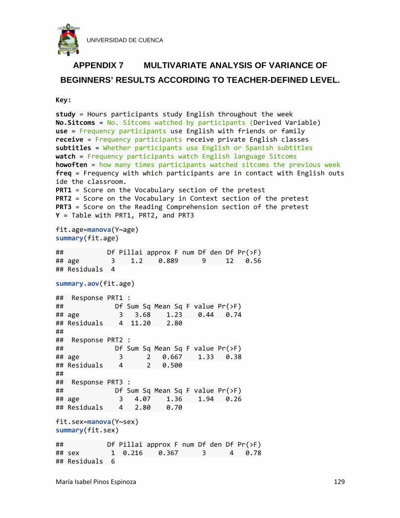
María Isabel Pinos Espinoza 129
UNIVERSIDAD DE CUENCA
APPENDIX 7 MULTIVARIATE ANALYSIS OF VARIANCE OF BEGINNERS’ RESULTS ACCORDING TO TEACHER-DEFINED LEVEL.
Key:
study = Hours participants study English throughout the week No.Sitcoms = No. Sitcoms watched by participants (Derived Variable) use = Frequency participants use English with friends or family receive = Frequency participants receive private English classes subtitles = Whether participants use English or Spanish subtitles watch = Frequency participants watch English language Sitcoms howoften = how many times participants watched sitcoms the previous week freq = Frequency with which participants are in contact with English outside the classroom. PRT1 = Score on the Vocabulary section of the pretest PRT2 = Score on the Vocabulary in Context section of the pretest PRT3 = Score on the Reading Comprehension section of the pretest Y = Table with PRT1, PRT2, and PRT3
fit.age=manova(Y~age) summary(fit.age)
## Df Pillai approx F num Df den Df Pr(>F) ## age 3 1.2 0.889 9 12 0.56 ## Residuals 4
summary.aov(fit.age)
## Response PRT1 : ## Df Sum Sq Mean Sq F value Pr(>F) ## age 3 3.68 1.23 0.44 0.74 ## Residuals 4 11.20 2.80 ## ## Response PRT2 : ## Df Sum Sq Mean Sq F value Pr(>F) ## age 3 2 0.667 1.33 0.38 ## Residuals 4 2 0.500 ## ## Response PRT3 : ## Df Sum Sq Mean Sq F value Pr(>F) ## age 3 4.07 1.36 1.94 0.26 ## Residuals 4 2.80 0.70
fit.sex=manova(Y~sex) summary(fit.sex)
## Df Pillai approx F num Df den Df Pr(>F) ## sex 1 0.216 0.367 3 4 0.78 ## Residuals 6
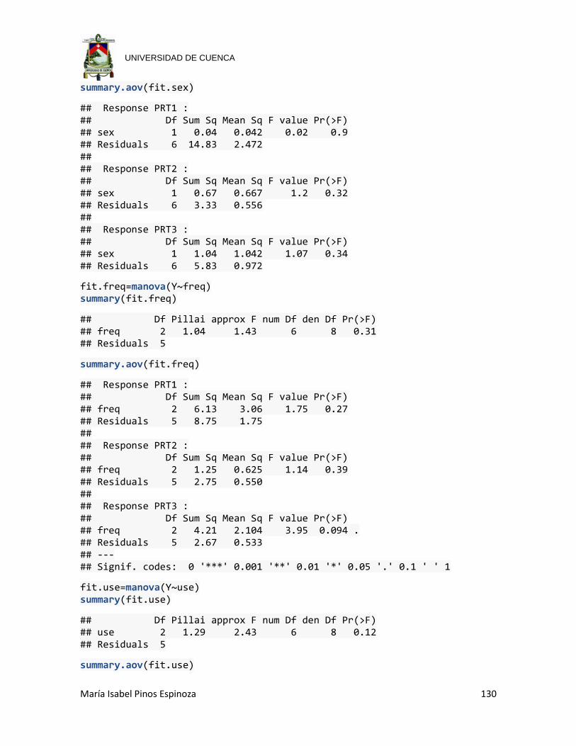
María Isabel Pinos Espinoza 130
UNIVERSIDAD DE CUENCA
summary.aov(fit.sex)
## Response PRT1 : ## Df Sum Sq Mean Sq F value Pr(>F) ## sex 1 0.04 0.042 0.02 0.9 ## Residuals 6 14.83 2.472 ## ## Response PRT2 : ## Df Sum Sq Mean Sq F value Pr(>F) ## sex 1 0.67 0.667 1.2 0.32 ## Residuals 6 3.33 0.556 ## ## Response PRT3 : ## Df Sum Sq Mean Sq F value Pr(>F) ## sex 1 1.04 1.042 1.07 0.34 ## Residuals 6 5.83 0.972
fit.freq=manova(Y~freq) summary(fit.freq)
## Df Pillai approx F num Df den Df Pr(>F) ## freq 2 1.04 1.43 6 8 0.31 ## Residuals 5
summary.aov(fit.freq)
## Response PRT1 : ## Df Sum Sq Mean Sq F value Pr(>F) ## freq 2 6.13 3.06 1.75 0.27 ## Residuals 5 8.75 1.75 ## ## Response PRT2 : ## Df Sum Sq Mean Sq F value Pr(>F) ## freq 2 1.25 0.625 1.14 0.39 ## Residuals 5 2.75 0.550 ## ## Response PRT3 : ## Df Sum Sq Mean Sq F value Pr(>F) ## freq 2 4.21 2.104 3.95 0.094 . ## Residuals 5 2.67 0.533 ## --- ## Signif. codes: 0 '***' 0.001 '**' 0.01 '*' 0.05 '.' 0.1 ' ' 1
fit.use=manova(Y~use) summary(fit.use)
## Df Pillai approx F num Df den Df Pr(>F) ## use 2 1.29 2.43 6 8 0.12 ## Residuals 5
summary.aov(fit.use)
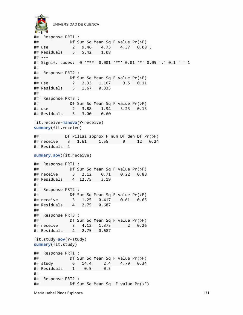
María Isabel Pinos Espinoza 131
UNIVERSIDAD DE CUENCA
## Response PRT1 : ## Df Sum Sq Mean Sq F value Pr(>F) ## use 2 9.46 4.73 4.37 0.08 . ## Residuals 5 5.42 1.08 ## --- ## Signif. codes: 0 '***' 0.001 '**' 0.01 '*' 0.05 '.' 0.1 ' ' 1 ## ## Response PRT2 : ## Df Sum Sq Mean Sq F value Pr(>F) ## use 2 2.33 1.167 3.5 0.11 ## Residuals 5 1.67 0.333 ## ## Response PRT3 : ## Df Sum Sq Mean Sq F value Pr(>F) ## use 2 3.88 1.94 3.23 0.13 ## Residuals 5 3.00 0.60
fit.receive=manova(Y~receive) summary(fit.receive)
## Df Pillai approx F num Df den Df Pr(>F) ## receive 3 1.61 1.55 9 12 0.24 ## Residuals 4
summary.aov(fit.receive)
## Response PRT1 : ## Df Sum Sq Mean Sq F value Pr(>F) ## receive 3 2.12 0.71 0.22 0.88 ## Residuals 4 12.75 3.19 ## ## Response PRT2 : ## Df Sum Sq Mean Sq F value Pr(>F) ## receive 3 1.25 0.417 0.61 0.65 ## Residuals 4 2.75 0.687 ## ## Response PRT3 : ## Df Sum Sq Mean Sq F value Pr(>F) ## receive 3 4.12 1.375 2 0.26 ## Residuals 4 2.75 0.687
fit.study=aov(Y~study) summary(fit.study)
## Response PRT1 : ## Df Sum Sq Mean Sq F value Pr(>F) ## study 6 14.4 2.4 4.79 0.34 ## Residuals 1 0.5 0.5 ## ## Response PRT2 : ## Df Sum Sq Mean Sq F value Pr(>F)

María Isabel Pinos Espinoza 132
UNIVERSIDAD DE CUENCA
## study 6 4 0.667 8.65e+32 <2e-16 *** ## Residuals 1 0 0.000 ## --- ## Signif. codes: 0 '***' 0.001 '**' 0.01 '*' 0.05 '.' 0.1 ' ' 1 ## ## Response PRT3 : ## Df Sum Sq Mean Sq F value Pr(>F) ## study 6 6.37 1.06 2.12 0.48 ## Residuals 1 0.50 0.50
fit.watch=manova(Y~watch) summary(fit.watch)
## Df Pillai approx F num Df den Df Pr(>F) ## watch 2 1.07 1.55 6 8 0.28 ## Residuals 5
summary.aov(fit.watch)
## Response PRT1 : ## Df Sum Sq Mean Sq F value Pr(>F) ## watch 2 9.88 4.94 4.94 0.066 . ## Residuals 5 5.00 1.00 ## --- ## Signif. codes: 0 '***' 0.001 '**' 0.01 '*' 0.05 '.' 0.1 ' ' 1 ## ## Response PRT2 : ## Df Sum Sq Mean Sq F value Pr(>F) ## watch 2 2.33 1.167 3.5 0.11 ## Residuals 5 1.67 0.333 ## ## Response PRT3 : ## Df Sum Sq Mean Sq F value Pr(>F) ## watch 2 0.21 0.104 0.08 0.93 ## Residuals 5 6.67 1.333
fit.subtitles=manova(Y~subtitles) summary(fit.subtitles)
## Df Pillai approx F num Df den Df Pr(>F) ## subtitles 2 1.4 3.12 6 8 0.07 . ## Residuals 5 ## --- ## Signif. codes: 0 '***' 0.001 '**' 0.01 '*' 0.05 '.' 0.1 ' ' 1
summary.aov(fit.subtitles)
## Response PRT1 : ## Df Sum Sq Mean Sq F value Pr(>F) ## subtitles 2 11.4 5.69 8.12 0.027 * ## Residuals 5 3.5 0.70

María Isabel Pinos Espinoza 133
UNIVERSIDAD DE CUENCA
## --- ## Signif. codes: 0 '***' 0.001 '**' 0.01 '*' 0.05 '.' 0.1 ' ' 1 ## ## Response PRT2 : ## Df Sum Sq Mean Sq F value Pr(>F) ## subtitles 2 2 1.0 2.5 0.18 ## Residuals 5 2 0.4 ## ## Response PRT3 : ## Df Sum Sq Mean Sq F value Pr(>F) ## subtitles 2 1.54 0.771 0.72 0.53 ## Residuals 5 5.33 1.067
fit.howoften=manova(Y~howoften) summary(fit.howoften)
## Df Pillai approx F num Df den Df Pr(>F) ## howoften 2 0.967 1.25 6 8 0.38 ## Residuals 5
summary.aov(fit.howoften)
## Response PRT1 : ## Df Sum Sq Mean Sq F value Pr(>F) ## howoften 2 1.46 0.729 0.27 0.77 ## Residuals 5 13.42 2.683 ## ## Response PRT2 : ## Df Sum Sq Mean Sq F value Pr(>F) ## howoften 2 2.33 1.167 3.5 0.11 ## Residuals 5 1.67 0.333 ## ## Response PRT3 : ## Df Sum Sq Mean Sq F value Pr(>F) ## howoften 2 5.21 2.604 7.81 0.029 * ## Residuals 5 1.67 0.333 ## --- ## Signif. codes: 0 '***' 0.001 '**' 0.01 '*' 0.05 '.' 0.1 ' ' 1
fit.sitcoms=manova(Y~No.Sitcoms) summary(fit.sitcoms)
## Df Pillai approx F num Df den Df Pr(>F) ## No.Sitcoms 2 1.16 1.82 6 8 0.21 ## Residuals 5
summary.aov(fit.sitcoms)
## Response PRT1 : ## Df Sum Sq Mean Sq F value Pr(>F) ## No.Sitcoms 2 9.54 4.77 4.47 0.077 .
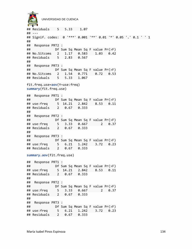
María Isabel Pinos Espinoza 134
UNIVERSIDAD DE CUENCA
## Residuals 5 5.33 1.07 ## --- ## Signif. codes: 0 '***' 0.001 '**' 0.01 '*' 0.05 '.' 0.1 ' ' 1 ## ## Response PRT2 : ## Df Sum Sq Mean Sq F value Pr(>F) ## No.Sitcoms 2 1.17 0.583 1.03 0.42 ## Residuals 5 2.83 0.567 ## ## Response PRT3 : ## Df Sum Sq Mean Sq F value Pr(>F) ## No.Sitcoms 2 1.54 0.771 0.72 0.53 ## Residuals 5 5.33 1.067
fit.freq.use=aov(Y~use:freq) summary(fit.freq.use)
## Response PRT1 : ## Df Sum Sq Mean Sq F value Pr(>F) ## use:freq 5 14.21 2.842 8.53 0.11 ## Residuals 2 0.67 0.333 ## ## Response PRT2 : ## Df Sum Sq Mean Sq F value Pr(>F) ## use:freq 5 3.33 0.667 2 0.37 ## Residuals 2 0.67 0.333 ## ## Response PRT3 : ## Df Sum Sq Mean Sq F value Pr(>F) ## use:freq 5 6.21 1.242 3.72 0.23 ## Residuals 2 0.67 0.333
summary.aov(fit.freq.use)
## Response PRT1 : ## Df Sum Sq Mean Sq F value Pr(>F) ## use:freq 5 14.21 2.842 8.53 0.11 ## Residuals 2 0.67 0.333 ## ## Response PRT2 : ## Df Sum Sq Mean Sq F value Pr(>F) ## use:freq 5 3.33 0.667 2 0.37 ## Residuals 2 0.67 0.333 ## ## Response PRT3 : ## Df Sum Sq Mean Sq F value Pr(>F) ## use:freq 5 6.21 1.242 3.72 0.23 ## Residuals 2 0.67 0.333

María Isabel Pinos Espinoza 135
UNIVERSIDAD DE CUENCA
fit.receive.study=aov(Y~receive:study) summary(fit.receive.study)
## Response PRT1 : ## Df Sum Sq Mean Sq F value Pr(>F) ## receive:study 6 14.4 2.4 4.79 0.34 ## Residuals 1 0.5 0.5 ## ## Response PRT2 : ## Df Sum Sq Mean Sq F value Pr(>F) ## receive:study 6 4 0.667 8.65e+32 <2e-16 *** ## Residuals 1 0 0.000 ## --- ## Signif. codes: 0 '***' 0.001 '**' 0.01 '*' 0.05 '.' 0.1 ' ' 1 ## ## Response PRT3 : ## Df Sum Sq Mean Sq F value Pr(>F) ## receive:study 6 6.38 1.06 2.13 0.48 ## Residuals 1 0.50 0.50
summary.aov(fit.receive.study)
## Response PRT1 : ## Df Sum Sq Mean Sq F value Pr(>F) ## receive:study 6 14.4 2.4 4.79 0.34 ## Residuals 1 0.5 0.5 ## ## Response PRT2 : ## Df Sum Sq Mean Sq F value Pr(>F) ## receive:study 6 4 0.667 8.65e+32 <2e-16 *** ## Residuals 1 0 0.000 ## --- ## Signif. codes: 0 '***' 0.001 '**' 0.01 '*' 0.05 '.' 0.1 ' ' 1 ## ## Response PRT3 : ## Df Sum Sq Mean Sq F value Pr(>F) ## receive:study 6 6.38 1.06 2.13 0.48 ## Residuals 1 0.50 0.50
fit.sitcom=manova(Y~howoften:No.Sitcoms) summary(fit.sitcom)
## Df Pillai approx F num Df den Df Pr(>F) ## howoften:No.Sitcoms 4 2.12 1.82 12 9 0.19 ## Residuals 3
summary.aov(fit.sitcom)
## Response PRT1 : ## Df Sum Sq Mean Sq F value Pr(>F) ## howoften:No.Sitcoms 4 12.21 3.052 3.43 0.17
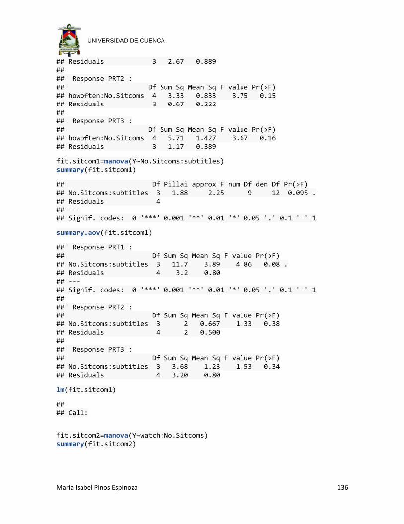
María Isabel Pinos Espinoza 136
UNIVERSIDAD DE CUENCA
## Residuals 3 2.67 0.889 ## ## Response PRT2 : ## Df Sum Sq Mean Sq F value Pr(>F) ## howoften:No.Sitcoms 4 3.33 0.833 3.75 0.15 ## Residuals 3 0.67 0.222 ## ## Response PRT3 : ## Df Sum Sq Mean Sq F value Pr(>F) ## howoften:No.Sitcoms 4 5.71 1.427 3.67 0.16 ## Residuals 3 1.17 0.389
fit.sitcom1=manova(Y~No.Sitcoms:subtitles) summary(fit.sitcom1)
## Df Pillai approx F num Df den Df Pr(>F) ## No.Sitcoms:subtitles 3 1.88 2.25 9 12 0.095 . ## Residuals 4 ## --- ## Signif. codes: 0 '***' 0.001 '**' 0.01 '*' 0.05 '.' 0.1 ' ' 1
summary.aov(fit.sitcom1)
## Response PRT1 : ## Df Sum Sq Mean Sq F value Pr(>F) ## No.Sitcoms:subtitles 3 11.7 3.89 4.86 0.08 . ## Residuals 4 3.2 0.80 ## --- ## Signif. codes: 0 '***' 0.001 '**' 0.01 '*' 0.05 '.' 0.1 ' ' 1 ## ## Response PRT2 : ## Df Sum Sq Mean Sq F value Pr(>F) ## No.Sitcoms:subtitles 3 2 0.667 1.33 0.38 ## Residuals 4 2 0.500 ## ## Response PRT3 : ## Df Sum Sq Mean Sq F value Pr(>F) ## No.Sitcoms:subtitles 3 3.68 1.23 1.53 0.34 ## Residuals 4 3.20 0.80
lm(fit.sitcom1)
## ## Call:
fit.sitcom2=manova(Y~watch:No.Sitcoms) summary(fit.sitcom2)
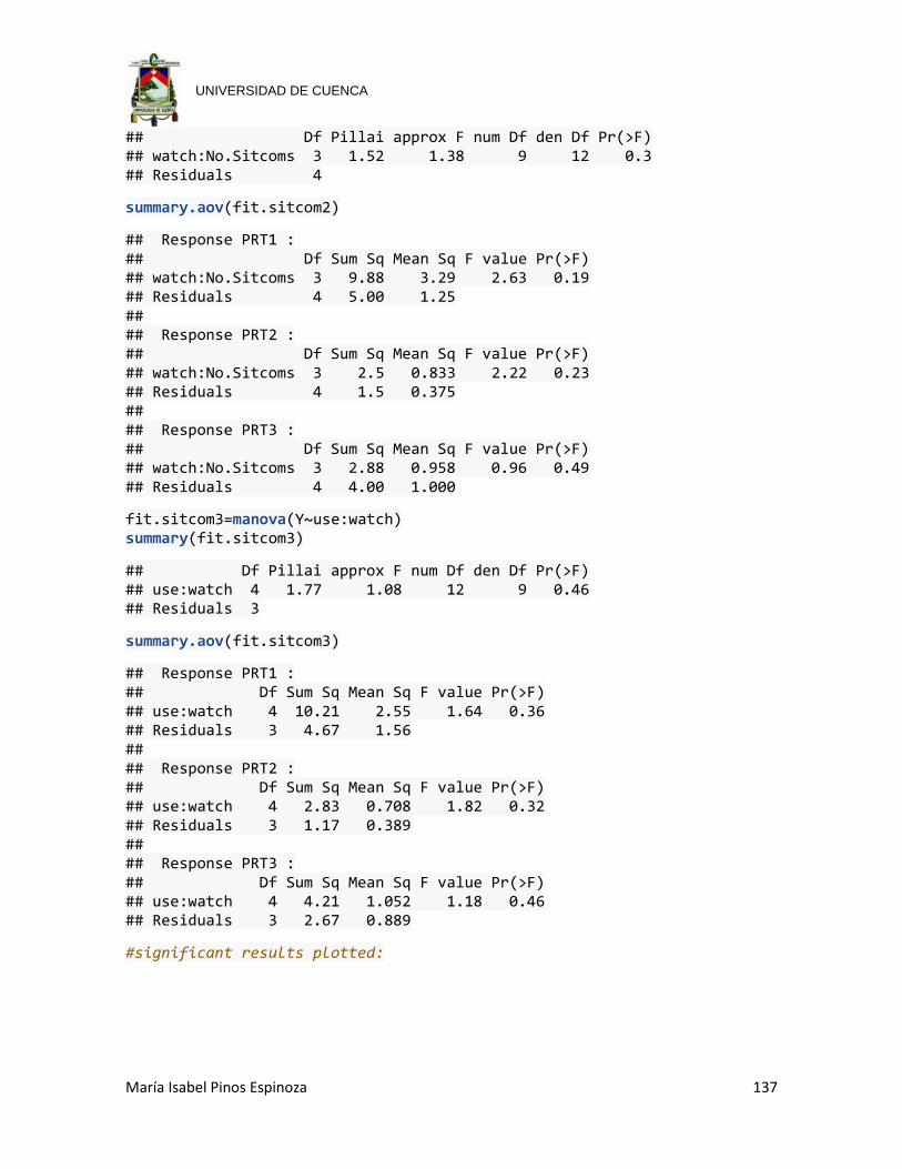
María Isabel Pinos Espinoza 137
UNIVERSIDAD DE CUENCA
## Df Pillai approx F num Df den Df Pr(>F) ## watch:No.Sitcoms 3 1.52 1.38 9 12 0.3 ## Residuals 4
summary.aov(fit.sitcom2)
## Response PRT1 : ## Df Sum Sq Mean Sq F value Pr(>F) ## watch:No.Sitcoms 3 9.88 3.29 2.63 0.19 ## Residuals 4 5.00 1.25 ## ## Response PRT2 : ## Df Sum Sq Mean Sq F value Pr(>F) ## watch:No.Sitcoms 3 2.5 0.833 2.22 0.23 ## Residuals 4 1.5 0.375 ## ## Response PRT3 : ## Df Sum Sq Mean Sq F value Pr(>F) ## watch:No.Sitcoms 3 2.88 0.958 0.96 0.49 ## Residuals 4 4.00 1.000
fit.sitcom3=manova(Y~use:watch) summary(fit.sitcom3)
## Df Pillai approx F num Df den Df Pr(>F) ## use:watch 4 1.77 1.08 12 9 0.46 ## Residuals 3
summary.aov(fit.sitcom3)
## Response PRT1 : ## Df Sum Sq Mean Sq F value Pr(>F) ## use:watch 4 10.21 2.55 1.64 0.36 ## Residuals 3 4.67 1.56 ## ## Response PRT2 : ## Df Sum Sq Mean Sq F value Pr(>F) ## use:watch 4 2.83 0.708 1.82 0.32 ## Residuals 3 1.17 0.389 ## ## Response PRT3 : ## Df Sum Sq Mean Sq F value Pr(>F) ## use:watch 4 4.21 1.052 1.18 0.46 ## Residuals 3 2.67 0.889
#significant results plotted:
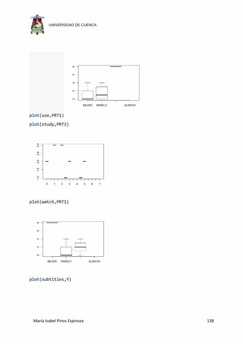
María Isabel Pinos Espinoza 138
UNIVERSIDAD DE CUENCA
plot(use,PRT1)
plot(study,PRT2)
plot(watch,PRT1)
plot(subtitles,Y)
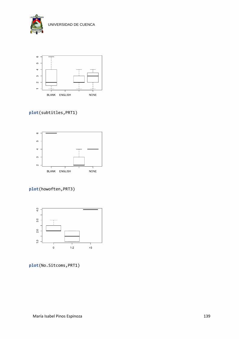
María Isabel Pinos Espinoza 139
UNIVERSIDAD DE CUENCA
plot(subtitles,PRT1)
plot(howoften,PRT3)
plot(No.Sitcoms,PRT1)

María Isabel Pinos Espinoza 140
UNIVERSIDAD DE CUENCA
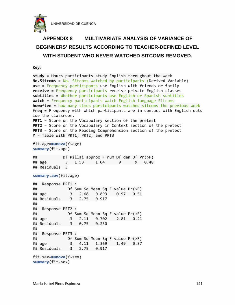
María Isabel Pinos Espinoza 141
UNIVERSIDAD DE CUENCA
APPENDIX 8 MULTIVARIATE ANALYSIS OF VARIANCE OF BEGINNERS’ RESULTS ACCORDING TO TEACHER-DEFINED LEVEL
WITH STUDENT WHO NEVER WATCHED SITCOMS REMOVED.
Key:
study = Hours participants study English throughout the week No.Sitcoms = No. Sitcoms watched by participants (Derived Variable) use = Frequency participants use English with friends or family receive = Frequency participants receive private English classes subtitles = Whether participants use English or Spanish subtitles watch = Frequency participants watch English language Sitcoms howoften = how many times participants watched sitcoms the previous week freq = Frequency with which participants are in contact with English outside the classroom. PRT1 = Score on the Vocabulary section of the pretest PRT2 = Score on the Vocabulary in Context section of the pretest PRT3 = Score on the Reading Comprehension section of the pretest Y = Table with PRT1, PRT2, and PRT3
fit.age=manova(Y~age) summary(fit.age)
## Df Pillai approx F num Df den Df Pr(>F) ## age 3 1.53 1.04 9 9 0.48 ## Residuals 3
summary.aov(fit.age)
## Response PRT1 : ## Df Sum Sq Mean Sq F value Pr(>F) ## age 3 2.68 0.893 0.97 0.51 ## Residuals 3 2.75 0.917 ## ## Response PRT2 : ## Df Sum Sq Mean Sq F value Pr(>F) ## age 3 2.11 0.702 2.81 0.21 ## Residuals 3 0.75 0.250 ## ## Response PRT3 : ## Df Sum Sq Mean Sq F value Pr(>F) ## age 3 4.11 1.369 1.49 0.37 ## Residuals 3 2.75 0.917
fit.sex=manova(Y~sex) summary(fit.sex)

María Isabel Pinos Espinoza 142
UNIVERSIDAD DE CUENCA
## Df Pillai approx F num Df den Df Pr(>F) ## sex 1 0.238 0.313 3 3 0.82 ## Residuals 5
summary.aov(fit.sex)
## Response PRT1 : ## Df Sum Sq Mean Sq F value Pr(>F) ## sex 1 0.23 0.229 0.22 0.66 ## Residuals 5 5.20 1.040 ## ## Response PRT2 : ## Df Sum Sq Mean Sq F value Pr(>F) ## sex 1 0.357 0.357 0.71 0.44 ## Residuals 5 2.500 0.500 ## ## Response PRT3 : ## Df Sum Sq Mean Sq F value Pr(>F) ## sex 1 1.16 1.16 1.02 0.36 ## Residuals 5 5.70 1.14
fit.freq=manova(Y~freq) summary(fit.freq)
## Df Pillai approx F num Df den Df Pr(>F) ## freq 2 1.13 1.3 6 6 0.38 ## Residuals 4
summary.aov(fit.freq)
## Response PRT1 : ## Df Sum Sq Mean Sq F value Pr(>F) ## freq 2 2.68 1.339 1.95 0.26 ## Residuals 4 2.75 0.688 ## ## Response PRT2 : ## Df Sum Sq Mean Sq F value Pr(>F) ## freq 2 1.61 0.804 2.57 0.19 ## Residuals 4 1.25 0.313 ## ## Response PRT3 : ## Df Sum Sq Mean Sq F value Pr(>F) ## freq 2 4.36 2.179 3.49 0.13 ## Residuals 4 2.50 0.625
fit.use=manova(Y~use) summary(fit.use)
## Df Pillai approx F num Df den Df Pr(>F) ## use 1 0.602 1.51 3 3 0.37 ## Residuals 5

María Isabel Pinos Espinoza 143
UNIVERSIDAD DE CUENCA
summary.aov(fit.use)
## Response PRT1 : ## Df Sum Sq Mean Sq F value Pr(>F) ## use 1 0.01 0.012 0.01 0.92 ## Residuals 5 5.42 1.083 ## ## Response PRT2 : ## Df Sum Sq Mean Sq F value Pr(>F) ## use 1 1.19 1.190 3.57 0.12 ## Residuals 5 1.67 0.333 ## ## Response PRT3 : ## Df Sum Sq Mean Sq F value Pr(>F) ## use 1 3.86 3.86 6.43 0.052 . ## Residuals 5 3.00 0.60 ## --- ## Signif. codes: 0 '***' 0.001 '**' 0.01 '*' 0.05 '.' 0.1 ' ' 1
fit.receive=aov(Y~receive) summary(fit.receive)
## Response PRT1 : ## Df Sum Sq Mean Sq F value Pr(>F) ## receive 3 2.76 0.921 1.04 0.49 ## Residuals 3 2.67 0.889 ## ## Response PRT2 : ## Df Sum Sq Mean Sq F value Pr(>F) ## receive 3 0.857 0.286 0.43 0.75 ## Residuals 3 2.000 0.667 ## ## Response PRT3 : ## Df Sum Sq Mean Sq F value Pr(>F) ## receive 3 4.19 1.397 1.57 0.36 ## Residuals 3 2.67 0.889
fit.study=aov(Y~study) summary(fit.study)
## Response PRT1 : ## Df Sum Sq Mean Sq F value Pr(>F) ## study 1 0.15 0.149 0.14 0.72 ## Residuals 5 5.28 1.056 ## ## Response PRT2 : ## Df Sum Sq Mean Sq F value Pr(>F) ## study 1 0.553 0.553 1.2 0.32 ## Residuals 5 2.304 0.461 ##

María Isabel Pinos Espinoza 144
UNIVERSIDAD DE CUENCA
## Response PRT3 : ## Df Sum Sq Mean Sq F value Pr(>F) ## study 1 2.43 2.432 2.75 0.16 ## Residuals 5 4.43 0.885
fit.watch=manova(Y~watch) summary(fit.watch)
## Df Pillai approx F num Df den Df Pr(>F) ## watch 1 0.602 1.51 3 3 0.37 ## Residuals 5
summary.aov(fit.watch)
## Response PRT1 : ## Df Sum Sq Mean Sq F value Pr(>F) ## watch 1 0.43 0.429 0.43 0.54 ## Residuals 5 5.00 1.000 ## ## Response PRT2 : ## Df Sum Sq Mean Sq F value Pr(>F) ## watch 1 1.19 1.190 3.57 0.12 ## Residuals 5 1.67 0.333 ## ## Response PRT3 : ## Df Sum Sq Mean Sq F value Pr(>F) ## watch 1 0.19 0.19 0.14 0.72 ## Residuals 5 6.67 1.33
fit.subtitles=manova(Y~subtitles) summary(fit.subtitles)
## Df Pillai approx F num Df den Df Pr(>F) ## subtitles 1 0.801 4.03 3 3 0.14 ## Residuals 5
summary.aov(fit.subtitles)
## Response PRT1 : ## Df Sum Sq Mean Sq F value Pr(>F) ## subtitles 1 1.93 1.93 2.76 0.16 ## Residuals 5 3.50 0.70 ## ## Response PRT2 : ## Df Sum Sq Mean Sq F value Pr(>F) ## subtitles 1 0.857 0.857 2.14 0.2 ## Residuals 5 2.000 0.400 ## ## Response PRT3 : ## Df Sum Sq Mean Sq F value Pr(>F)
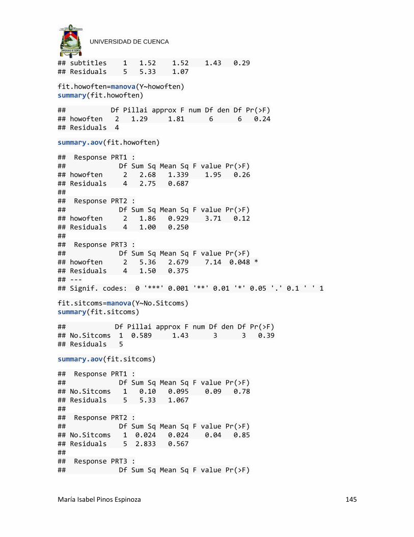
María Isabel Pinos Espinoza 145
UNIVERSIDAD DE CUENCA
## subtitles 1 1.52 1.52 1.43 0.29 ## Residuals 5 5.33 1.07
fit.howoften=manova(Y~howoften) summary(fit.howoften)
## Df Pillai approx F num Df den Df Pr(>F) ## howoften 2 1.29 1.81 6 6 0.24 ## Residuals 4
summary.aov(fit.howoften)
## Response PRT1 : ## Df Sum Sq Mean Sq F value Pr(>F) ## howoften 2 2.68 1.339 1.95 0.26 ## Residuals 4 2.75 0.687 ## ## Response PRT2 : ## Df Sum Sq Mean Sq F value Pr(>F) ## howoften 2 1.86 0.929 3.71 0.12 ## Residuals 4 1.00 0.250 ## ## Response PRT3 : ## Df Sum Sq Mean Sq F value Pr(>F) ## howoften 2 5.36 2.679 7.14 0.048 * ## Residuals 4 1.50 0.375 ## --- ## Signif. codes: 0 '***' 0.001 '**' 0.01 '*' 0.05 '.' 0.1 ' ' 1
fit.sitcoms=manova(Y~No.Sitcoms) summary(fit.sitcoms)
## Df Pillai approx F num Df den Df Pr(>F) ## No.Sitcoms 1 0.589 1.43 3 3 0.39 ## Residuals 5
summary.aov(fit.sitcoms)
## Response PRT1 : ## Df Sum Sq Mean Sq F value Pr(>F) ## No.Sitcoms 1 0.10 0.095 0.09 0.78 ## Residuals 5 5.33 1.067 ## ## Response PRT2 : ## Df Sum Sq Mean Sq F value Pr(>F) ## No.Sitcoms 1 0.024 0.024 0.04 0.85 ## Residuals 5 2.833 0.567 ## ## Response PRT3 : ## Df Sum Sq Mean Sq F value Pr(>F)
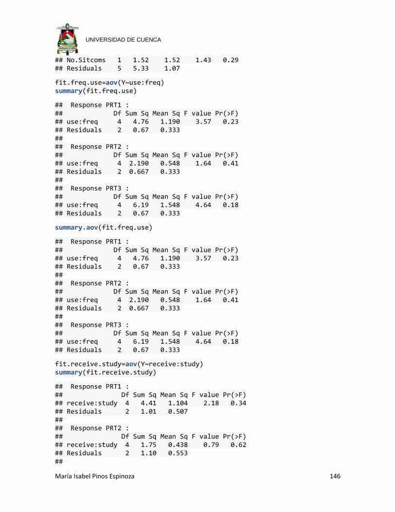
María Isabel Pinos Espinoza 146
UNIVERSIDAD DE CUENCA
## No.Sitcoms 1 1.52 1.52 1.43 0.29 ## Residuals 5 5.33 1.07
fit.freq.use=aov(Y~use:freq) summary(fit.freq.use)
## Response PRT1 : ## Df Sum Sq Mean Sq F value Pr(>F) ## use:freq 4 4.76 1.190 3.57 0.23 ## Residuals 2 0.67 0.333 ## ## Response PRT2 : ## Df Sum Sq Mean Sq F value Pr(>F) ## use:freq 4 2.190 0.548 1.64 0.41 ## Residuals 2 0.667 0.333 ## ## Response PRT3 : ## Df Sum Sq Mean Sq F value Pr(>F) ## use:freq 4 6.19 1.548 4.64 0.18 ## Residuals 2 0.67 0.333
summary.aov(fit.freq.use)
## Response PRT1 : ## Df Sum Sq Mean Sq F value Pr(>F) ## use:freq 4 4.76 1.190 3.57 0.23 ## Residuals 2 0.67 0.333 ## ## Response PRT2 : ## Df Sum Sq Mean Sq F value Pr(>F) ## use:freq 4 2.190 0.548 1.64 0.41 ## Residuals 2 0.667 0.333 ## ## Response PRT3 : ## Df Sum Sq Mean Sq F value Pr(>F) ## use:freq 4 6.19 1.548 4.64 0.18 ## Residuals 2 0.67 0.333
fit.receive.study=aov(Y~receive:study) summary(fit.receive.study)
## Response PRT1 : ## Df Sum Sq Mean Sq F value Pr(>F) ## receive:study 4 4.41 1.104 2.18 0.34 ## Residuals 2 1.01 0.507 ## ## Response PRT2 : ## Df Sum Sq Mean Sq F value Pr(>F) ## receive:study 4 1.75 0.438 0.79 0.62 ## Residuals 2 1.10 0.553 ##

María Isabel Pinos Espinoza 147
UNIVERSIDAD DE CUENCA
## Response PRT3 : ## Df Sum Sq Mean Sq F value Pr(>F) ## receive:study 4 6.35 1.589 6.33 0.14 ## Residuals 2 0.50 0.251
summary.aov(fit.receive.study)
## Response PRT1 : ## Df Sum Sq Mean Sq F value Pr(>F) ## receive:study 4 4.41 1.104 2.18 0.34 ## Residuals 2 1.01 0.507 ## ## Response PRT2 : ## Df Sum Sq Mean Sq F value Pr(>F) ## receive:study 4 1.75 0.438 0.79 0.62 ## Residuals 2 1.10 0.553 ## ## Response PRT3 : ## Df Sum Sq Mean Sq F value Pr(>F) ## receive:study 4 6.35 1.589 6.33 0.14 ## Residuals 2 0.50 0.251
fit.sitcom=manova(Y~howoften:No.Sitcoms) summary(fit.sitcom)
## Df Pillai approx F num Df den Df Pr(>F) ## howoften:No.Sitcoms 3 1.84 1.58 9 9 0.25 ## Residuals 3
summary.aov(fit.sitcom)
## Response PRT1 : ## Df Sum Sq Mean Sq F value Pr(>F) ## howoften:No.Sitcoms 3 2.76 0.921 1.04 0.49 ## Residuals 3 2.67 0.889 ## ## Response PRT2 : ## Df Sum Sq Mean Sq F value Pr(>F) ## howoften:No.Sitcoms 3 2.190 0.730 3.29 0.18 ## Residuals 3 0.667 0.222 ## ## Response PRT3 : ## Df Sum Sq Mean Sq F value Pr(>F) ## howoften:No.Sitcoms 3 5.69 1.897 4.88 0.11 ## Residuals 3 1.17 0.389
fit.sitcom1=manova(Y~No.Sitcoms:subtitles) summary(fit.sitcom1)

María Isabel Pinos Espinoza 148
UNIVERSIDAD DE CUENCA
## Df Pillai approx F num Df den Df Pr(>F) ## No.Sitcoms:subtitles 2 1.45 2.64 6 6 0.13 ## Residuals 4
summary.aov(fit.sitcom1)
## Response PRT1 : ## Df Sum Sq Mean Sq F value Pr(>F) ## No.Sitcoms:subtitles 2 2.23 1.11 1.39 0.35 ## Residuals 4 3.20 0.80 ## ## Response PRT2 : ## Df Sum Sq Mean Sq F value Pr(>F) ## No.Sitcoms:subtitles 2 0.857 0.429 0.86 0.49 ## Residuals 4 2.000 0.500 ## ## Response PRT3 : ## Df Sum Sq Mean Sq F value Pr(>F) ## No.Sitcoms:subtitles 2 3.66 1.83 2.29 0.22 ## Residuals 4 3.20 0.80
fit.sitcom2=manova(Y~watch:No.Sitcoms) summary(fit.sitcom2)
## Df Pillai approx F num Df den Df Pr(>F) ## watch:No.Sitcoms 2 1.07 1.16 6 6 0.43 ## Residuals 4
summary.aov(fit.sitcom2)
## Response PRT1 : ## Df Sum Sq Mean Sq F value Pr(>F) ## watch:No.Sitcoms 2 0.43 0.214 0.17 0.85 ## Residuals 4 5.00 1.250 ## ## Response PRT2 : ## Df Sum Sq Mean Sq F value Pr(>F) ## watch:No.Sitcoms 2 1.36 0.679 1.81 0.28 ## Residuals 4 1.50 0.375 ## ## Response PRT3 : ## Df Sum Sq Mean Sq F value Pr(>F) ## watch:No.Sitcoms 2 2.86 1.43 1.43 0.34 ## Residuals 4 4.00 1.00
fit.sitcom3=manova(Y~use:watch) summary(fit.sitcom3)
## Df Pillai approx F num Df den Df Pr(>F) ## use:watch 3 1.35 0.819 9 9 0.61 ## Residuals 3
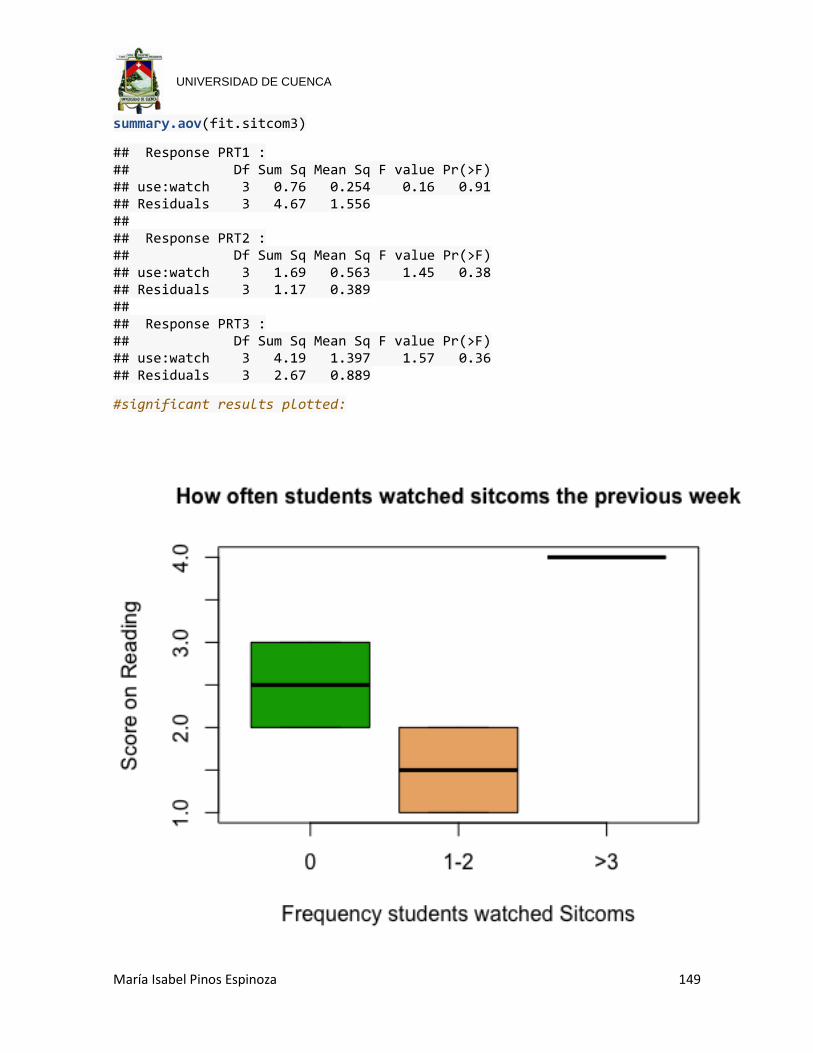
María Isabel Pinos Espinoza 149
UNIVERSIDAD DE CUENCA
summary.aov(fit.sitcom3)
## Response PRT1 : ## Df Sum Sq Mean Sq F value Pr(>F) ## use:watch 3 0.76 0.254 0.16 0.91 ## Residuals 3 4.67 1.556 ## ## Response PRT2 : ## Df Sum Sq Mean Sq F value Pr(>F) ## use:watch 3 1.69 0.563 1.45 0.38 ## Residuals 3 1.17 0.389 ## ## Response PRT3 : ## Df Sum Sq Mean Sq F value Pr(>F) ## use:watch 3 4.19 1.397 1.57 0.36 ## Residuals 3 2.67 0.889
#significant results plotted:

María Isabel Pinos Espinoza 150
UNIVERSIDAD DE CUENCA
APPENDIX 9 MULTIVARIATE ANALYSIS OF VARIANCE OF INTERMEDIATES’ RESULTS ACCORDING TO TEACHER-DEFINED LEVEL.
Key:
study = Hours participants study English throughout the week No.Sitcoms = No. Sitcoms watched by participants (Derived Variable) use = Frequency participants use English with friends or family receive = Frequency participants receive private English classes subtitles = Whether participants use English or Spanish subtitles watch = Frequency participants watch English language Sitcoms howoften = how many times participants watched sitcoms the previous week freq = Frequency with which participants are in contact with English outside the classroom. PRT1 = Score on the Vocabulary section of the pretest PRT2 = Score on the Vocabulary in Context section of the pretest PRT3 = Score on the Reading Comprehension section of the pretest Y = Table with PRT1, PRT2, and PRT3
fit.age=manova(Y~age) summary(fit.age)
## Df Pillai approx F num Df den Df Pr(>F) ## age 3 0.339 0.382 9 27 0.93 ## Residuals 9
summary.aov(fit.age)
## Response PRT1 : ## Df Sum Sq Mean Sq F value Pr(>F) ## age 3 4.5 1.52 0.4 0.76 ## Residuals 9 34.4 3.82 ## ## Response PRT2 : ## Df Sum Sq Mean Sq F value Pr(>F) ## age 3 1.19 0.397 0.19 0.9 ## Residuals 9 18.50 2.056 ## ## Response PRT3 : ## Df Sum Sq Mean Sq F value Pr(>F) ## age 3 1.81 0.603 0.43 0.73 ## Residuals 9 12.50 1.389
fit.sex=manova(Y~sex) summary(fit.sex)
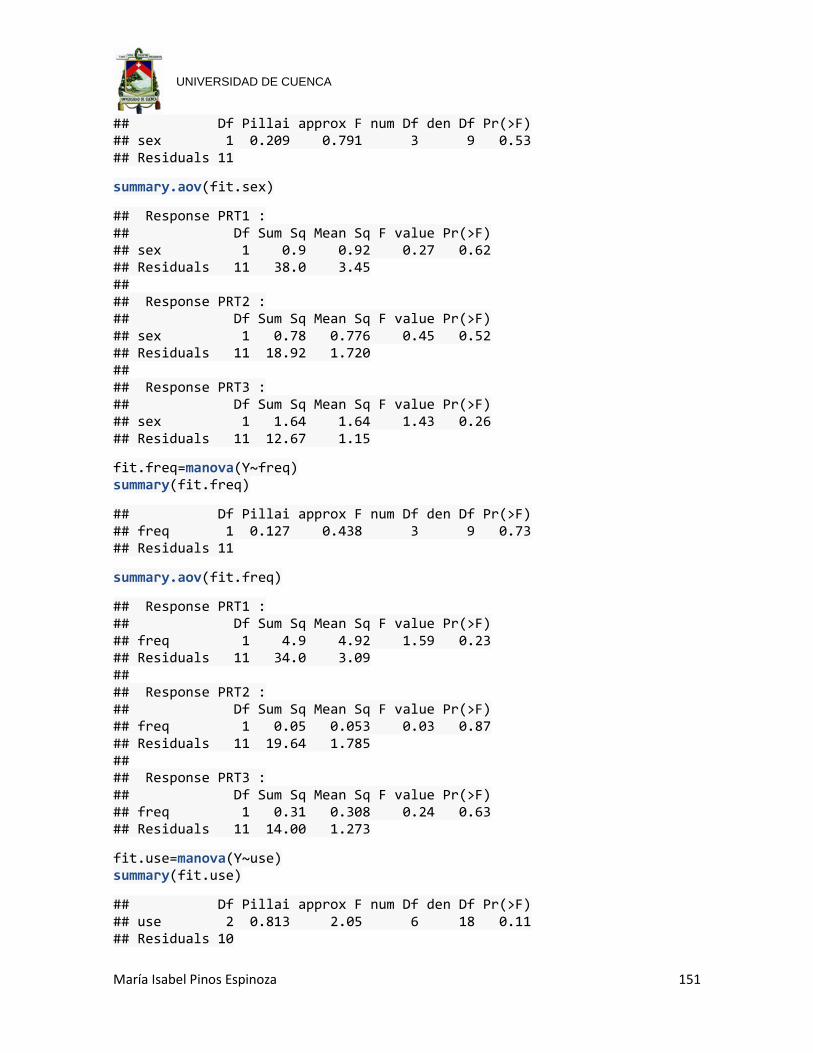
María Isabel Pinos Espinoza 151
UNIVERSIDAD DE CUENCA
## Df Pillai approx F num Df den Df Pr(>F) ## sex 1 0.209 0.791 3 9 0.53 ## Residuals 11
summary.aov(fit.sex)
## Response PRT1 : ## Df Sum Sq Mean Sq F value Pr(>F) ## sex 1 0.9 0.92 0.27 0.62 ## Residuals 11 38.0 3.45 ## ## Response PRT2 : ## Df Sum Sq Mean Sq F value Pr(>F) ## sex 1 0.78 0.776 0.45 0.52 ## Residuals 11 18.92 1.720 ## ## Response PRT3 : ## Df Sum Sq Mean Sq F value Pr(>F) ## sex 1 1.64 1.64 1.43 0.26 ## Residuals 11 12.67 1.15
fit.freq=manova(Y~freq) summary(fit.freq)
## Df Pillai approx F num Df den Df Pr(>F) ## freq 1 0.127 0.438 3 9 0.73 ## Residuals 11
summary.aov(fit.freq)
## Response PRT1 : ## Df Sum Sq Mean Sq F value Pr(>F) ## freq 1 4.9 4.92 1.59 0.23 ## Residuals 11 34.0 3.09 ## ## Response PRT2 : ## Df Sum Sq Mean Sq F value Pr(>F) ## freq 1 0.05 0.053 0.03 0.87 ## Residuals 11 19.64 1.785 ## ## Response PRT3 : ## Df Sum Sq Mean Sq F value Pr(>F) ## freq 1 0.31 0.308 0.24 0.63 ## Residuals 11 14.00 1.273
fit.use=manova(Y~use) summary(fit.use)
## Df Pillai approx F num Df den Df Pr(>F) ## use 2 0.813 2.05 6 18 0.11 ## Residuals 10
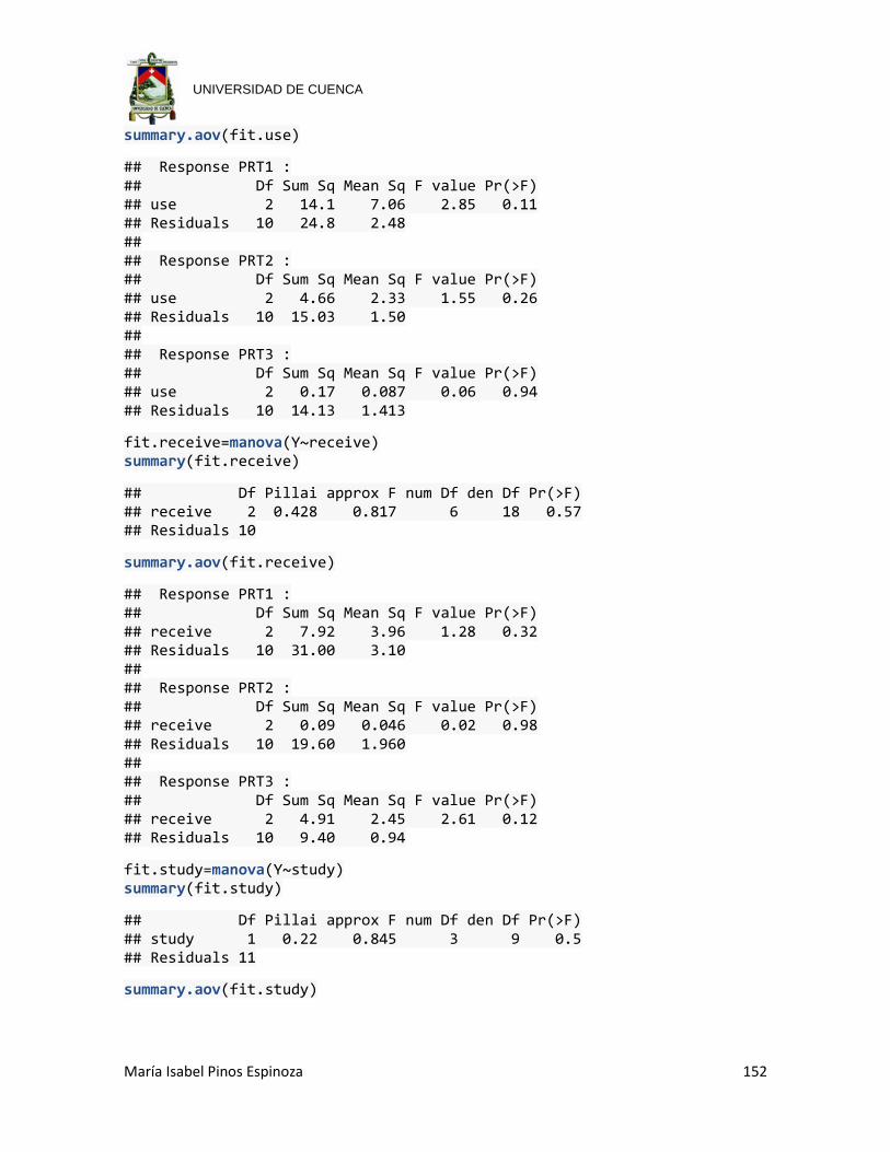
María Isabel Pinos Espinoza 152
UNIVERSIDAD DE CUENCA
summary.aov(fit.use)
## Response PRT1 : ## Df Sum Sq Mean Sq F value Pr(>F) ## use 2 14.1 7.06 2.85 0.11 ## Residuals 10 24.8 2.48 ## ## Response PRT2 : ## Df Sum Sq Mean Sq F value Pr(>F) ## use 2 4.66 2.33 1.55 0.26 ## Residuals 10 15.03 1.50 ## ## Response PRT3 : ## Df Sum Sq Mean Sq F value Pr(>F) ## use 2 0.17 0.087 0.06 0.94 ## Residuals 10 14.13 1.413
fit.receive=manova(Y~receive) summary(fit.receive)
## Df Pillai approx F num Df den Df Pr(>F) ## receive 2 0.428 0.817 6 18 0.57 ## Residuals 10
summary.aov(fit.receive)
## Response PRT1 : ## Df Sum Sq Mean Sq F value Pr(>F) ## receive 2 7.92 3.96 1.28 0.32 ## Residuals 10 31.00 3.10 ## ## Response PRT2 : ## Df Sum Sq Mean Sq F value Pr(>F) ## receive 2 0.09 0.046 0.02 0.98 ## Residuals 10 19.60 1.960 ## ## Response PRT3 : ## Df Sum Sq Mean Sq F value Pr(>F) ## receive 2 4.91 2.45 2.61 0.12 ## Residuals 10 9.40 0.94
fit.study=manova(Y~study) summary(fit.study)
## Df Pillai approx F num Df den Df Pr(>F) ## study 1 0.22 0.845 3 9 0.5 ## Residuals 11
summary.aov(fit.study)
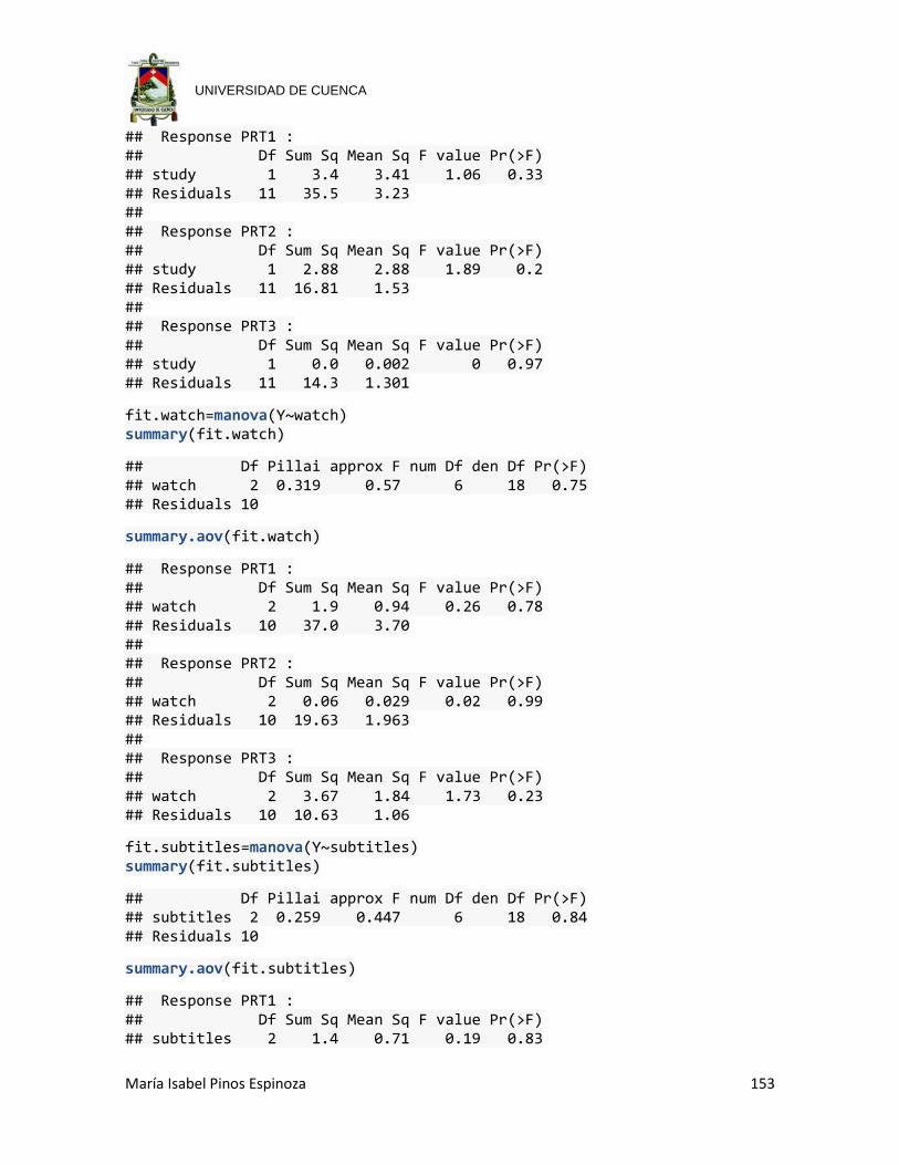
María Isabel Pinos Espinoza 153
UNIVERSIDAD DE CUENCA
## Response PRT1 : ## Df Sum Sq Mean Sq F value Pr(>F) ## study 1 3.4 3.41 1.06 0.33 ## Residuals 11 35.5 3.23 ## ## Response PRT2 : ## Df Sum Sq Mean Sq F value Pr(>F) ## study 1 2.88 2.88 1.89 0.2 ## Residuals 11 16.81 1.53 ## ## Response PRT3 : ## Df Sum Sq Mean Sq F value Pr(>F) ## study 1 0.0 0.002 0 0.97 ## Residuals 11 14.3 1.301
fit.watch=manova(Y~watch) summary(fit.watch)
## Df Pillai approx F num Df den Df Pr(>F) ## watch 2 0.319 0.57 6 18 0.75 ## Residuals 10
summary.aov(fit.watch)
## Response PRT1 : ## Df Sum Sq Mean Sq F value Pr(>F) ## watch 2 1.9 0.94 0.26 0.78 ## Residuals 10 37.0 3.70 ## ## Response PRT2 : ## Df Sum Sq Mean Sq F value Pr(>F) ## watch 2 0.06 0.029 0.02 0.99 ## Residuals 10 19.63 1.963 ## ## Response PRT3 : ## Df Sum Sq Mean Sq F value Pr(>F) ## watch 2 3.67 1.84 1.73 0.23 ## Residuals 10 10.63 1.06
fit.subtitles=manova(Y~subtitles) summary(fit.subtitles)
## Df Pillai approx F num Df den Df Pr(>F) ## subtitles 2 0.259 0.447 6 18 0.84 ## Residuals 10
summary.aov(fit.subtitles)
## Response PRT1 : ## Df Sum Sq Mean Sq F value Pr(>F) ## subtitles 2 1.4 0.71 0.19 0.83

María Isabel Pinos Espinoza 154
UNIVERSIDAD DE CUENCA
## Residuals 10 37.5 3.75 ## ## Response PRT2 : ## Df Sum Sq Mean Sq F value Pr(>F) ## subtitles 2 2.07 1.03 0.59 0.57 ## Residuals 10 17.63 1.76 ## ## Response PRT3 : ## Df Sum Sq Mean Sq F value Pr(>F) ## subtitles 2 2.68 1.34 1.15 0.35 ## Residuals 10 11.62 1.16
fit.howoften=manova(Y~howoften) summary(fit.howoften)
## Df Pillai approx F num Df den Df Pr(>F) ## howoften 2 0.25 0.429 6 18 0.85 ## Residuals 10
summary.aov(fit.howoften)
## Response PRT1 : ## Df Sum Sq Mean Sq F value Pr(>F) ## howoften 2 1.5 0.76 0.2 0.82 ## Residuals 10 37.4 3.74 ## ## Response PRT2 : ## Df Sum Sq Mean Sq F value Pr(>F) ## howoften 2 0.79 0.396 0.21 0.81 ## Residuals 10 18.90 1.890 ## ## Response PRT3 : ## Df Sum Sq Mean Sq F value Pr(>F) ## howoften 2 1.71 0.854 0.68 0.53 ## Residuals 10 12.60 1.260
fit.sitcoms=manova(Y~No.Sitcoms) summary(fit.sitcoms)
## Df Pillai approx F num Df den Df Pr(>F) ## No.Sitcoms 4 0.912 0.874 12 24 0.58 ## Residuals 8
summary.aov(fit.sitcoms)
## Response PRT1 : ## Df Sum Sq Mean Sq F value Pr(>F) ## No.Sitcoms 4 11.5 2.88 0.84 0.54 ## Residuals 8 27.4 3.43 ## ## Response PRT2 :
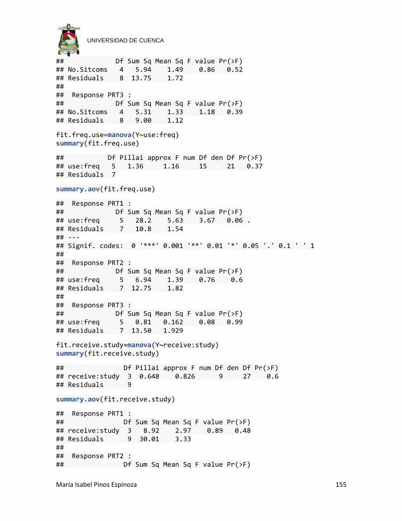
María Isabel Pinos Espinoza 155
UNIVERSIDAD DE CUENCA
## Df Sum Sq Mean Sq F value Pr(>F) ## No.Sitcoms 4 5.94 1.49 0.86 0.52 ## Residuals 8 13.75 1.72 ## ## Response PRT3 : ## Df Sum Sq Mean Sq F value Pr(>F) ## No.Sitcoms 4 5.31 1.33 1.18 0.39 ## Residuals 8 9.00 1.12
fit.freq.use=manova(Y~use:freq) summary(fit.freq.use)
## Df Pillai approx F num Df den Df Pr(>F) ## use:freq 5 1.36 1.16 15 21 0.37 ## Residuals 7
summary.aov(fit.freq.use)
## Response PRT1 : ## Df Sum Sq Mean Sq F value Pr(>F) ## use:freq 5 28.2 5.63 3.67 0.06 . ## Residuals 7 10.8 1.54 ## --- ## Signif. codes: 0 '***' 0.001 '**' 0.01 '*' 0.05 '.' 0.1 ' ' 1 ## ## Response PRT2 : ## Df Sum Sq Mean Sq F value Pr(>F) ## use:freq 5 6.94 1.39 0.76 0.6 ## Residuals 7 12.75 1.82 ## ## Response PRT3 : ## Df Sum Sq Mean Sq F value Pr(>F) ## use:freq 5 0.81 0.162 0.08 0.99 ## Residuals 7 13.50 1.929
fit.receive.study=manova(Y~receive:study) summary(fit.receive.study)
## Df Pillai approx F num Df den Df Pr(>F) ## receive:study 3 0.648 0.826 9 27 0.6 ## Residuals 9
summary.aov(fit.receive.study)
## Response PRT1 : ## Df Sum Sq Mean Sq F value Pr(>F) ## receive:study 3 8.92 2.97 0.89 0.48 ## Residuals 9 30.01 3.33 ## ## Response PRT2 : ## Df Sum Sq Mean Sq F value Pr(>F)
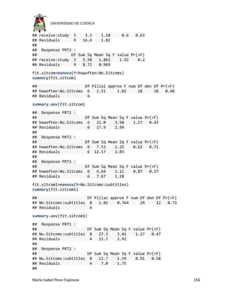
María Isabel Pinos Espinoza 156
UNIVERSIDAD DE CUENCA
## receive:study 3 3.3 1.10 0.6 0.63 ## Residuals 9 16.4 1.82 ## ## Response PRT3 : ## Df Sum Sq Mean Sq F value Pr(>F) ## receive:study 3 5.58 1.861 1.92 0.2 ## Residuals 9 8.72 0.969
fit.sitcom=manova(Y~howoften:No.Sitcoms) summary(fit.sitcom)
## Df Pillai approx F num Df den Df Pr(>F) ## howoften:No.Sitcoms 6 1.51 1.02 18 18 0.48 ## Residuals 6
summary.aov(fit.sitcom)
## Response PRT1 : ## Df Sum Sq Mean Sq F value Pr(>F) ## howoften:No.Sitcoms 6 21.0 3.50 1.17 0.43 ## Residuals 6 17.9 2.99 ## ## Response PRT2 : ## Df Sum Sq Mean Sq F value Pr(>F) ## howoften:No.Sitcoms 6 7.53 1.25 0.62 0.71 ## Residuals 6 12.17 2.03 ## ## Response PRT3 : ## Df Sum Sq Mean Sq F value Pr(>F) ## howoften:No.Sitcoms 6 6.64 1.11 0.87 0.57 ## Residuals 6 7.67 1.28
fit.sitcom1=manova(Y~No.Sitcoms:subtitles) summary(fit.sitcom1)
## Df Pillai approx F num Df den Df Pr(>F) ## No.Sitcoms:subtitles 8 1.81 0.764 24 12 0.72 ## Residuals 4
summary.aov(fit.sitcom1)
## Response PRT1 : ## Df Sum Sq Mean Sq F value Pr(>F) ## No.Sitcoms:subtitles 8 27.3 3.41 1.17 0.47 ## Residuals 4 11.7 2.92 ## ## Response PRT2 : ## Df Sum Sq Mean Sq F value Pr(>F) ## No.Sitcoms:subtitles 8 12.7 1.59 0.91 0.58 ## Residuals 4 7.0 1.75 ##
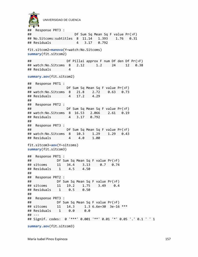
María Isabel Pinos Espinoza 157
UNIVERSIDAD DE CUENCA
## Response PRT3 : ## Df Sum Sq Mean Sq F value Pr(>F) ## No.Sitcoms:subtitles 8 11.14 1.393 1.76 0.31 ## Residuals 4 3.17 0.792
fit.sitcom2=manova(Y~watch:No.Sitcoms) summary(fit.sitcom2)
## Df Pillai approx F num Df den Df Pr(>F) ## watch:No.Sitcoms 8 2.12 1.2 24 12 0.38 ## Residuals 4
summary.aov(fit.sitcom2)
## Response PRT1 : ## Df Sum Sq Mean Sq F value Pr(>F) ## watch:No.Sitcoms 8 21.8 2.72 0.63 0.73 ## Residuals 4 17.2 4.29 ## ## Response PRT2 : ## Df Sum Sq Mean Sq F value Pr(>F) ## watch:No.Sitcoms 8 16.53 2.066 2.61 0.19 ## Residuals 4 3.17 0.792 ## ## Response PRT3 : ## Df Sum Sq Mean Sq F value Pr(>F) ## watch:No.Sitcoms 8 10.3 1.29 1.29 0.43 ## Residuals 4 4.0 1.00
fit.sitcom3=aov(Y~sitcoms) summary(fit.sitcom3)
## Response PRT1 : ## Df Sum Sq Mean Sq F value Pr(>F) ## sitcoms 11 34.4 3.13 0.7 0.74 ## Residuals 1 4.5 4.50 ## ## Response PRT2 : ## Df Sum Sq Mean Sq F value Pr(>F) ## sitcoms 11 19.2 1.75 3.49 0.4 ## Residuals 1 0.5 0.50 ## ## Response PRT3 : ## Df Sum Sq Mean Sq F value Pr(>F) ## sitcoms 11 14.3 1.3 6.6e+30 3e-16 *** ## Residuals 1 0.0 0.0 ## --- ## Signif. codes: 0 '***' 0.001 '**' 0.01 '*' 0.05 '.' 0.1 ' ' 1
summary.aov(fit.sitcom3)
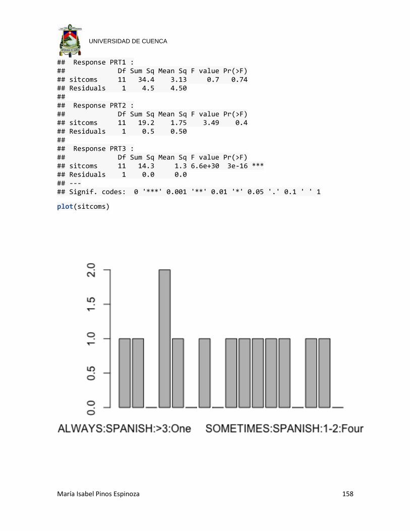
María Isabel Pinos Espinoza 158
UNIVERSIDAD DE CUENCA
## Response PRT1 : ## Df Sum Sq Mean Sq F value Pr(>F) ## sitcoms 11 34.4 3.13 0.7 0.74 ## Residuals 1 4.5 4.50 ## ## Response PRT2 : ## Df Sum Sq Mean Sq F value Pr(>F) ## sitcoms 11 19.2 1.75 3.49 0.4 ## Residuals 1 0.5 0.50 ## ## Response PRT3 : ## Df Sum Sq Mean Sq F value Pr(>F) ## sitcoms 11 14.3 1.3 6.6e+30 3e-16 *** ## Residuals 1 0.0 0.0 ## --- ## Signif. codes: 0 '***' 0.001 '**' 0.01 '*' 0.05 '.' 0.1 ' ' 1
plot(sitcoms)
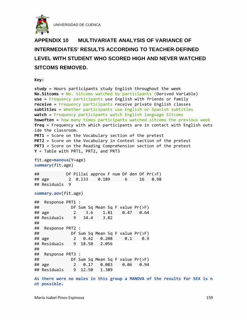
María Isabel Pinos Espinoza 159
UNIVERSIDAD DE CUENCA
APPENDIX 10 MULTIVARIATE ANALYSIS OF VARIANCE OF INTERMEDIATES’ RESULTS ACCORDING TO TEACHER-DEFINED LEVEL WITH STUDENT WHO SCORED HIGH AND NEVER WATCHED SITCOMS REMOVED.
Key:
study = Hours participants study English throughout the week No.Sitcoms = No. Sitcoms watched by participants (Derived Variable) use = Frequency participants use English with friends or family receive = Frequency participants receive private English classes subtitles = Whether participants use English or Spanish subtitles watch = Frequency participants watch English language Sitcoms howoften = how many times participants watched sitcoms the previous week freq = Frequency with which participants are in contact with English outside the classroom. PRT1 = Score on the Vocabulary section of the pretest PRT2 = Score on the Vocabulary in Context section of the pretest PRT3 = Score on the Reading Comprehension section of the pretest Y = Table with PRT1, PRT2, and PRT3
fit.age=manova(Y~age) summary(fit.age)
## Df Pillai approx F num Df den Df Pr(>F) ## age 2 0.133 0.189 6 16 0.98 ## Residuals 9
summary.aov(fit.age)
## Response PRT1 : ## Df Sum Sq Mean Sq F value Pr(>F) ## age 2 3.6 1.81 0.47 0.64 ## Residuals 9 34.4 3.82 ## ## Response PRT2 : ## Df Sum Sq Mean Sq F value Pr(>F) ## age 2 0.42 0.208 0.1 0.9 ## Residuals 9 18.50 2.056 ## ## Response PRT3 : ## Df Sum Sq Mean Sq F value Pr(>F) ## age 2 0.17 0.083 0.06 0.94 ## Residuals 9 12.50 1.389
As there were no males in this group a MANOVA of the results for SEX is not possible.

María Isabel Pinos Espinoza 160
UNIVERSIDAD DE CUENCA
fit.freq=manova(Y~freq) summary(fit.freq)
## Df Pillai approx F num Df den Df Pr(>F) ## freq 1 0.178 0.576 3 8 0.65 ## Residuals 10
summary.aov(fit.freq)
## Response PRT1 : ## Df Sum Sq Mean Sq F value Pr(>F) ## freq 1 6 6.0 1.88 0.2 ## Residuals 10 32 3.2 ## ## Response PRT2 : ## Df Sum Sq Mean Sq F value Pr(>F) ## freq 1 0.17 0.167 0.09 0.77 ## Residuals 10 18.75 1.875 ## ## Response PRT3 : ## Df Sum Sq Mean Sq F value Pr(>F) ## freq 1 0.67 0.667 0.56 0.47 ## Residuals 10 12.00 1.200
fit.use=manova(Y~use) summary(fit.use)
## Df Pillai approx F num Df den Df Pr(>F) ## use 2 0.776 1.69 6 16 0.19 ## Residuals 9
summary.aov(fit.use)
## Response PRT1 : ## Df Sum Sq Mean Sq F value Pr(>F) ## use 2 15.9 7.95 3.24 0.087 . ## Residuals 9 22.1 2.46 ## --- ## Signif. codes: 0 '***' 0.001 '**' 0.01 '*' 0.05 '.' 0.1 ' ' 1 ## ## Response PRT2 : ## Df Sum Sq Mean Sq F value Pr(>F) ## use 2 4.02 2.01 1.21 0.34 ## Residuals 9 14.90 1.66 ## ## Response PRT3 : ## Df Sum Sq Mean Sq F value Pr(>F) ## use 2 0.17 0.083 0.06 0.94 ## Residuals 9 12.50 1.389

María Isabel Pinos Espinoza 161
UNIVERSIDAD DE CUENCA
fit.receive=manova(Y~receive) summary(fit.receive)
## Df Pillai approx F num Df den Df Pr(>F) ## receive 2 0.428 0.726 6 16 0.64 ## Residuals 9
summary.aov(fit.receive)
## Response PRT1 : ## Df Sum Sq Mean Sq F value Pr(>F) ## receive 2 7.28 3.64 1.07 0.38 ## Residuals 9 30.72 3.41 ## ## Response PRT2 : ## Df Sum Sq Mean Sq F value Pr(>F) ## receive 2 0.03 0.014 0.01 0.99 ## Residuals 9 18.89 2.099 ## ## Response PRT3 : ## Df Sum Sq Mean Sq F value Pr(>F) ## receive 2 4.17 2.083 2.21 0.17 ## Residuals 9 8.50 0.944
fit.study=manova(Y~study) summary(fit.study)
## Df Pillai approx F num Df den Df Pr(>F) ## study 1 0.208 0.701 3 8 0.58 ## Residuals 10
summary.aov(fit.study)
## Response PRT1 : ## Df Sum Sq Mean Sq F value Pr(>F) ## study 1 3 3.03 0.87 0.37 ## Residuals 10 35 3.50 ## ## Response PRT2 : ## Df Sum Sq Mean Sq F value Pr(>F) ## study 1 2.57 2.57 1.57 0.24 ## Residuals 10 16.35 1.64 ## ## Response PRT3 : ## Df Sum Sq Mean Sq F value Pr(>F) ## study 1 0.01 0.012 0.01 0.92 ## Residuals 10 12.65 1.265
fit.watch=manova(Y~watch) summary(fit.watch)
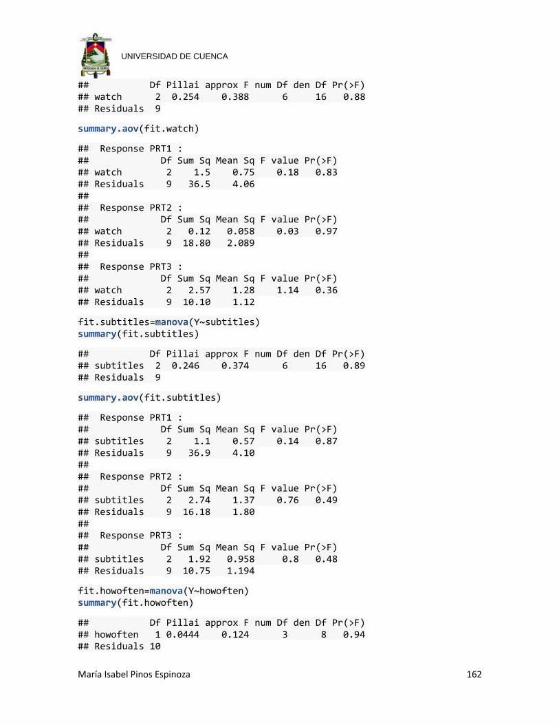
María Isabel Pinos Espinoza 162
UNIVERSIDAD DE CUENCA
## Df Pillai approx F num Df den Df Pr(>F) ## watch 2 0.254 0.388 6 16 0.88 ## Residuals 9
summary.aov(fit.watch)
## Response PRT1 : ## Df Sum Sq Mean Sq F value Pr(>F) ## watch 2 1.5 0.75 0.18 0.83 ## Residuals 9 36.5 4.06 ## ## Response PRT2 : ## Df Sum Sq Mean Sq F value Pr(>F) ## watch 2 0.12 0.058 0.03 0.97 ## Residuals 9 18.80 2.089 ## ## Response PRT3 : ## Df Sum Sq Mean Sq F value Pr(>F) ## watch 2 2.57 1.28 1.14 0.36 ## Residuals 9 10.10 1.12
fit.subtitles=manova(Y~subtitles) summary(fit.subtitles)
## Df Pillai approx F num Df den Df Pr(>F) ## subtitles 2 0.246 0.374 6 16 0.89 ## Residuals 9
summary.aov(fit.subtitles)
## Response PRT1 : ## Df Sum Sq Mean Sq F value Pr(>F) ## subtitles 2 1.1 0.57 0.14 0.87 ## Residuals 9 36.9 4.10 ## ## Response PRT2 : ## Df Sum Sq Mean Sq F value Pr(>F) ## subtitles 2 2.74 1.37 0.76 0.49 ## Residuals 9 16.18 1.80 ## ## Response PRT3 : ## Df Sum Sq Mean Sq F value Pr(>F) ## subtitles 2 1.92 0.958 0.8 0.48 ## Residuals 9 10.75 1.194
fit.howoften=manova(Y~howoften) summary(fit.howoften)
## Df Pillai approx F num Df den Df Pr(>F) ## howoften 1 0.0444 0.124 3 8 0.94 ## Residuals 10

María Isabel Pinos Espinoza 163
UNIVERSIDAD DE CUENCA
summary.aov(fit.howoften)
## Response PRT1 : ## Df Sum Sq Mean Sq F value Pr(>F) ## howoften 1 0.6 0.60 0.16 0.7 ## Residuals 10 37.4 3.74 ## ## Response PRT2 : ## Df Sum Sq Mean Sq F value Pr(>F) ## howoften 1 0.02 0.017 0.01 0.93 ## Residuals 10 18.90 1.890 ## ## Response PRT3 : ## Df Sum Sq Mean Sq F value Pr(>F) ## howoften 1 0.07 0.067 0.05 0.82 ## Residuals 10 12.60 1.260
fit.sitcoms=manova(Y~No.Sitcoms) summary(fit.sitcoms)
## Df Pillai approx F num Df den Df Pr(>F) ## No.Sitcoms 3 0.778 0.934 9 24 0.51 ## Residuals 8
summary.aov(fit.sitcoms)
## Response PRT1 : ## Df Sum Sq Mean Sq F value Pr(>F) ## No.Sitcoms 3 10.6 3.53 1.03 0.43 ## Residuals 8 27.4 3.43 ## ## Response PRT2 : ## Df Sum Sq Mean Sq F value Pr(>F) ## No.Sitcoms 3 5.17 1.72 1 0.44 ## Residuals 8 13.75 1.72 ## ## Response PRT3 : ## Df Sum Sq Mean Sq F value Pr(>F) ## No.Sitcoms 3 3.67 1.22 1.09 0.41 ## Residuals 8 9.00 1.12
fit.freq.use=manova(Y~use:freq) summary(fit.freq.use)
## Df Pillai approx F num Df den Df Pr(>F) ## use:freq 5 1.35 0.98 15 18 0.51 ## Residuals 6
summary.aov(fit.freq.use)
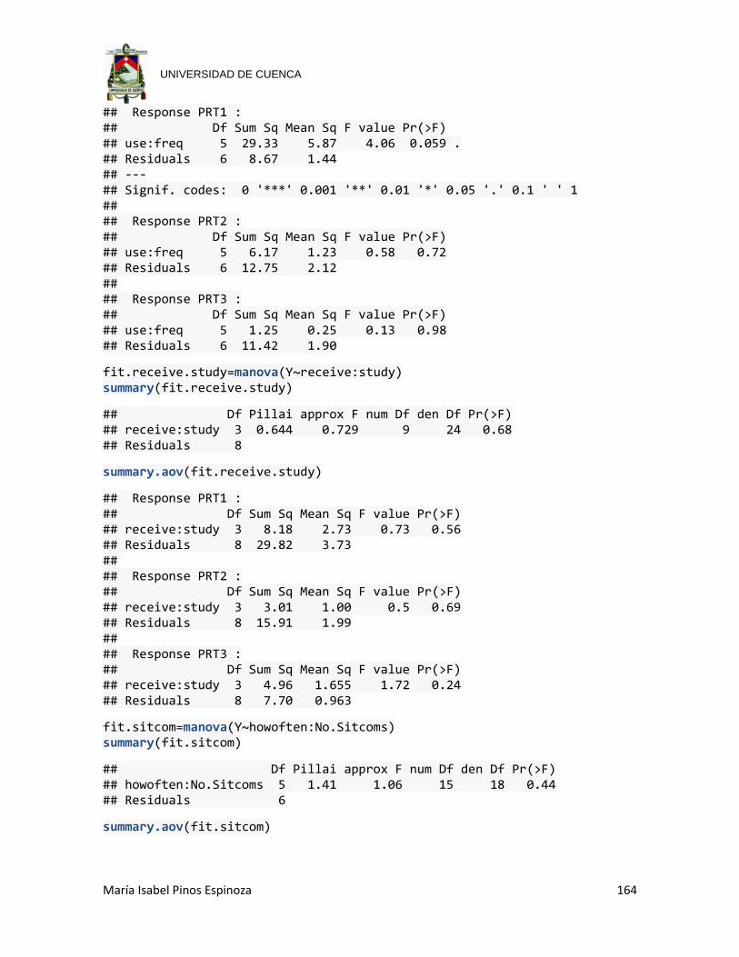
María Isabel Pinos Espinoza 164
UNIVERSIDAD DE CUENCA
## Response PRT1 : ## Df Sum Sq Mean Sq F value Pr(>F) ## use:freq 5 29.33 5.87 4.06 0.059 . ## Residuals 6 8.67 1.44 ## --- ## Signif. codes: 0 '***' 0.001 '**' 0.01 '*' 0.05 '.' 0.1 ' ' 1 ## ## Response PRT2 : ## Df Sum Sq Mean Sq F value Pr(>F) ## use:freq 5 6.17 1.23 0.58 0.72 ## Residuals 6 12.75 2.12 ## ## Response PRT3 : ## Df Sum Sq Mean Sq F value Pr(>F) ## use:freq 5 1.25 0.25 0.13 0.98 ## Residuals 6 11.42 1.90
fit.receive.study=manova(Y~receive:study) summary(fit.receive.study)
## Df Pillai approx F num Df den Df Pr(>F) ## receive:study 3 0.644 0.729 9 24 0.68 ## Residuals 8
summary.aov(fit.receive.study)
## Response PRT1 : ## Df Sum Sq Mean Sq F value Pr(>F) ## receive:study 3 8.18 2.73 0.73 0.56 ## Residuals 8 29.82 3.73 ## ## Response PRT2 : ## Df Sum Sq Mean Sq F value Pr(>F) ## receive:study 3 3.01 1.00 0.5 0.69 ## Residuals 8 15.91 1.99 ## ## Response PRT3 : ## Df Sum Sq Mean Sq F value Pr(>F) ## receive:study 3 4.96 1.655 1.72 0.24 ## Residuals 8 7.70 0.963
fit.sitcom=manova(Y~howoften:No.Sitcoms) summary(fit.sitcom)
## Df Pillai approx F num Df den Df Pr(>F) ## howoften:No.Sitcoms 5 1.41 1.06 15 18 0.44 ## Residuals 6
summary.aov(fit.sitcom)

María Isabel Pinos Espinoza 165
UNIVERSIDAD DE CUENCA
## Response PRT1 : ## Df Sum Sq Mean Sq F value Pr(>F) ## howoften:No.Sitcoms 5 20.1 4.02 1.35 0.36 ## Residuals 6 17.9 2.99 ## ## Response PRT2 : ## Df Sum Sq Mean Sq F value Pr(>F) ## howoften:No.Sitcoms 5 6.75 1.35 0.67 0.66 ## Residuals 6 12.17 2.03 ## ## Response PRT3 : ## Df Sum Sq Mean Sq F value Pr(>F) ## howoften:No.Sitcoms 5 5.00 1.00 0.78 0.6 ## Residuals 6 7.67 1.28
fit.sitcom1=manova(Y~No.Sitcoms:subtitles) summary(fit.sitcom1)
## Df Pillai approx F num Df den Df Pr(>F) ## No.Sitcoms:subtitles 7 1.73 0.781 21 12 0.7 ## Residuals 4
summary.aov(fit.sitcom1)
## Response PRT1 : ## Df Sum Sq Mean Sq F value Pr(>F) ## No.Sitcoms:subtitles 7 26.3 3.76 1.29 0.43 ## Residuals 4 11.7 2.92 ## ## Response PRT2 : ## Df Sum Sq Mean Sq F value Pr(>F) ## No.Sitcoms:subtitles 7 11.9 1.70 0.97 0.54 ## Residuals 4 7.0 1.75 ## ## Response PRT3 : ## Df Sum Sq Mean Sq F value Pr(>F) ## No.Sitcoms:subtitles 7 9.50 1.357 1.71 0.31 ## Residuals 4 3.17 0.792
fit.sitcom2=manova(Y~watch:No.Sitcoms) summary(fit.sitcom2)
## Df Pillai approx F num Df den Df Pr(>F) ## watch:No.Sitcoms 7 2.02 1.17 21 12 0.4 ## Residuals 4
summary.aov(fit.sitcom2)
## Response PRT1 : ## Df Sum Sq Mean Sq F value Pr(>F) ## watch:No.Sitcoms 7 20.8 2.98 0.69 0.69
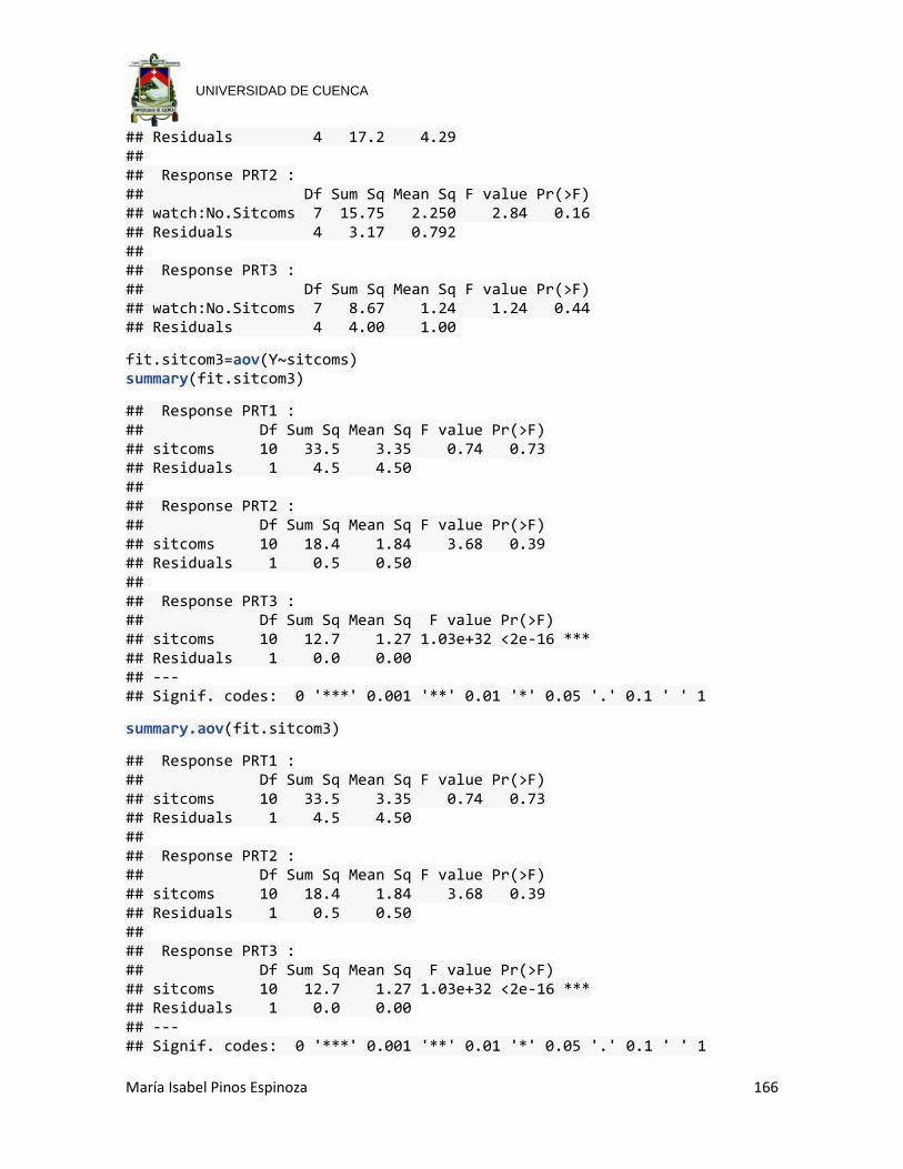
María Isabel Pinos Espinoza 166
UNIVERSIDAD DE CUENCA
## Residuals 4 17.2 4.29 ## ## Response PRT2 : ## Df Sum Sq Mean Sq F value Pr(>F) ## watch:No.Sitcoms 7 15.75 2.250 2.84 0.16 ## Residuals 4 3.17 0.792 ## ## Response PRT3 : ## Df Sum Sq Mean Sq F value Pr(>F) ## watch:No.Sitcoms 7 8.67 1.24 1.24 0.44 ## Residuals 4 4.00 1.00
fit.sitcom3=aov(Y~sitcoms) summary(fit.sitcom3)
## Response PRT1 : ## Df Sum Sq Mean Sq F value Pr(>F) ## sitcoms 10 33.5 3.35 0.74 0.73 ## Residuals 1 4.5 4.50 ## ## Response PRT2 : ## Df Sum Sq Mean Sq F value Pr(>F) ## sitcoms 10 18.4 1.84 3.68 0.39 ## Residuals 1 0.5 0.50 ## ## Response PRT3 : ## Df Sum Sq Mean Sq F value Pr(>F) ## sitcoms 10 12.7 1.27 1.03e+32 <2e-16 *** ## Residuals 1 0.0 0.00 ## --- ## Signif. codes: 0 '***' 0.001 '**' 0.01 '*' 0.05 '.' 0.1 ' ' 1
summary.aov(fit.sitcom3)
## Response PRT1 : ## Df Sum Sq Mean Sq F value Pr(>F) ## sitcoms 10 33.5 3.35 0.74 0.73 ## Residuals 1 4.5 4.50 ## ## Response PRT2 : ## Df Sum Sq Mean Sq F value Pr(>F) ## sitcoms 10 18.4 1.84 3.68 0.39 ## Residuals 1 0.5 0.50 ## ## Response PRT3 : ## Df Sum Sq Mean Sq F value Pr(>F) ## sitcoms 10 12.7 1.27 1.03e+32 <2e-16 *** ## Residuals 1 0.0 0.00 ## --- ## Signif. codes: 0 '***' 0.001 '**' 0.01 '*' 0.05 '.' 0.1 ' ' 1

María Isabel Pinos Espinoza 167
UNIVERSIDAD DE CUENCA
APPENDIX 11 MULTIVARIATE ANALYSIS OF VARIANCE OF ALL PARTICIPANTS RESULTS ACCORDING TO TEACHER-DEFINED LEVEL EXCEPT THE ADVANCED PARTICIPANT.
Key:
study = Hours participants study English throughout the week No.Sitcoms = No. Sitcoms watched by participants (Derived Variable) use = Frequency participants use English with friends or family receive = Frequency participants receive private English classes subtitles = Whether participants use English or Spanish subtitles watch = Frequency participants watch English language Sitcoms howoften = how many times participants watched sitcoms the previous week freq = Frequency with which participants are in contact with English outside the classroom. PRT1 = Score on the Vocabulary section of the pretest PRT2 = Score on the Vocabulary in Context section of the pretest PRT3 = Score on the Reading Comprehension section of the pretest Y = Table with PRT1, PRT2, and PRT3
fit.age=manova(Y~age) summary(fit.age)
## Df Pillai approx F num Df den Df Pr(>F) ## age 3 0.215 0.439 9 51 0.91 ## Residuals 17
summary.aov(fit.age)
## Response PRT1 : ## Df Sum Sq Mean Sq F value Pr(>F) ## age 3 4.1 1.38 0.25 0.86 ## Residuals 17 92.8 5.46 ## ## Response PRT2 : ## Df Sum Sq Mean Sq F value Pr(>F) ## age 3 1.1 0.366 0.16 0.92 ## Residuals 17 39.5 2.322 ## ## Response PRT3 : ## Df Sum Sq Mean Sq F value Pr(>F) ## age 3 3.8 1.27 0.92 0.45 ## Residuals 17 23.4 1.38
fit.sex=manova(Y~sex) summary(fit.sex)
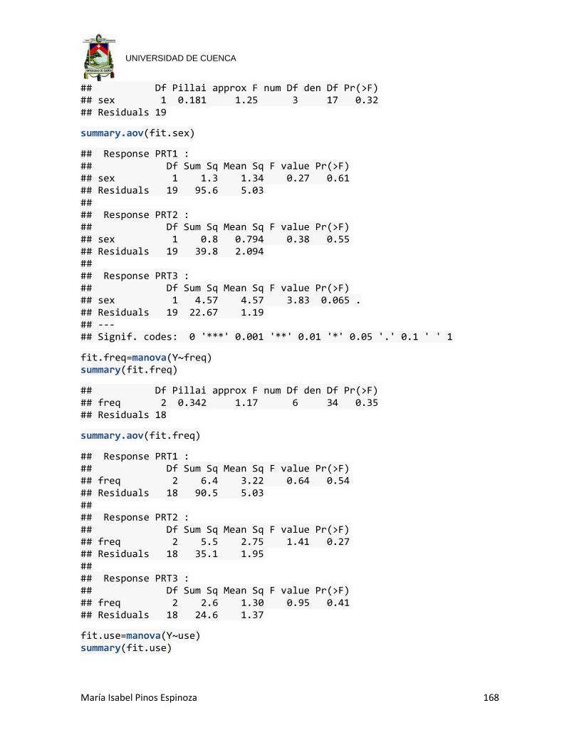
María Isabel Pinos Espinoza 168
UNIVERSIDAD DE CUENCA
## Df Pillai approx F num Df den Df Pr(>F) ## sex 1 0.181 1.25 3 17 0.32 ## Residuals 19
summary.aov(fit.sex)
## Response PRT1 : ## Df Sum Sq Mean Sq F value Pr(>F) ## sex 1 1.3 1.34 0.27 0.61 ## Residuals 19 95.6 5.03 ## ## Response PRT2 : ## Df Sum Sq Mean Sq F value Pr(>F) ## sex 1 0.8 0.794 0.38 0.55 ## Residuals 19 39.8 2.094 ## ## Response PRT3 : ## Df Sum Sq Mean Sq F value Pr(>F) ## sex 1 4.57 4.57 3.83 0.065 . ## Residuals 19 22.67 1.19 ## --- ## Signif. codes: 0 '***' 0.001 '**' 0.01 '*' 0.05 '.' 0.1 ' ' 1
fit.freq=manova(Y~freq) summary(fit.freq)
## Df Pillai approx F num Df den Df Pr(>F) ## freq 2 0.342 1.17 6 34 0.35 ## Residuals 18
summary.aov(fit.freq)
## Response PRT1 : ## Df Sum Sq Mean Sq F value Pr(>F) ## freq 2 6.4 3.22 0.64 0.54 ## Residuals 18 90.5 5.03 ## ## Response PRT2 : ## Df Sum Sq Mean Sq F value Pr(>F) ## freq 2 5.5 2.75 1.41 0.27 ## Residuals 18 35.1 1.95 ## ## Response PRT3 : ## Df Sum Sq Mean Sq F value Pr(>F) ## freq 2 2.6 1.30 0.95 0.41 ## Residuals 18 24.6 1.37
fit.use=manova(Y~use) summary(fit.use)
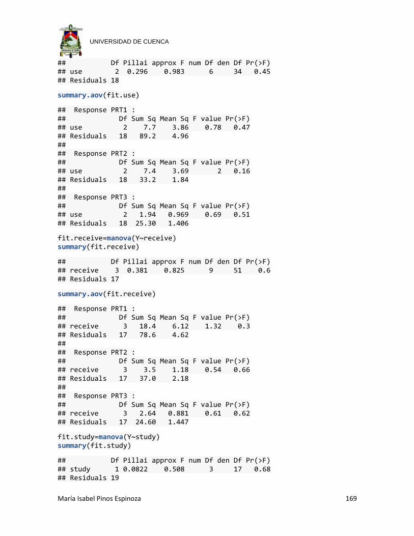
María Isabel Pinos Espinoza 169
UNIVERSIDAD DE CUENCA
## Df Pillai approx F num Df den Df Pr(>F) ## use 2 0.296 0.983 6 34 0.45 ## Residuals 18
summary.aov(fit.use)
## Response PRT1 : ## Df Sum Sq Mean Sq F value Pr(>F) ## use 2 7.7 3.86 0.78 0.47 ## Residuals 18 89.2 4.96 ## ## Response PRT2 : ## Df Sum Sq Mean Sq F value Pr(>F) ## use 2 7.4 3.69 2 0.16 ## Residuals 18 33.2 1.84 ## ## Response PRT3 : ## Df Sum Sq Mean Sq F value Pr(>F) ## use 2 1.94 0.969 0.69 0.51 ## Residuals 18 25.30 1.406
fit.receive=manova(Y~receive) summary(fit.receive)
## Df Pillai approx F num Df den Df Pr(>F) ## receive 3 0.381 0.825 9 51 0.6 ## Residuals 17
summary.aov(fit.receive)
## Response PRT1 : ## Df Sum Sq Mean Sq F value Pr(>F) ## receive 3 18.4 6.12 1.32 0.3 ## Residuals 17 78.6 4.62 ## ## Response PRT2 : ## Df Sum Sq Mean Sq F value Pr(>F) ## receive 3 3.5 1.18 0.54 0.66 ## Residuals 17 37.0 2.18 ## ## Response PRT3 : ## Df Sum Sq Mean Sq F value Pr(>F) ## receive 3 2.64 0.881 0.61 0.62 ## Residuals 17 24.60 1.447
fit.study=manova(Y~study) summary(fit.study)
## Df Pillai approx F num Df den Df Pr(>F) ## study 1 0.0822 0.508 3 17 0.68 ## Residuals 19
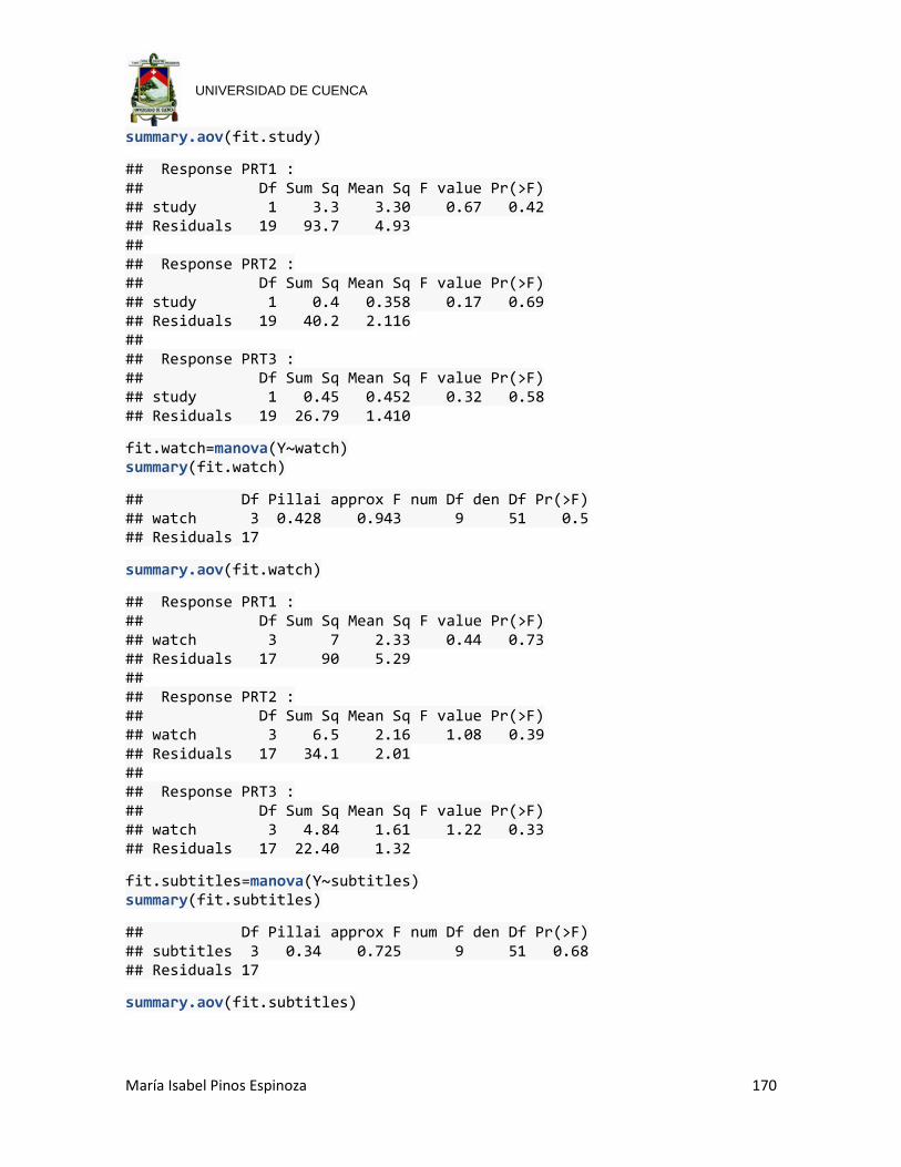
María Isabel Pinos Espinoza 170
UNIVERSIDAD DE CUENCA
summary.aov(fit.study)
## Response PRT1 : ## Df Sum Sq Mean Sq F value Pr(>F) ## study 1 3.3 3.30 0.67 0.42 ## Residuals 19 93.7 4.93 ## ## Response PRT2 : ## Df Sum Sq Mean Sq F value Pr(>F) ## study 1 0.4 0.358 0.17 0.69 ## Residuals 19 40.2 2.116 ## ## Response PRT3 : ## Df Sum Sq Mean Sq F value Pr(>F) ## study 1 0.45 0.452 0.32 0.58 ## Residuals 19 26.79 1.410
fit.watch=manova(Y~watch) summary(fit.watch)
## Df Pillai approx F num Df den Df Pr(>F) ## watch 3 0.428 0.943 9 51 0.5 ## Residuals 17
summary.aov(fit.watch)
## Response PRT1 : ## Df Sum Sq Mean Sq F value Pr(>F) ## watch 3 7 2.33 0.44 0.73 ## Residuals 17 90 5.29 ## ## Response PRT2 : ## Df Sum Sq Mean Sq F value Pr(>F) ## watch 3 6.5 2.16 1.08 0.39 ## Residuals 17 34.1 2.01 ## ## Response PRT3 : ## Df Sum Sq Mean Sq F value Pr(>F) ## watch 3 4.84 1.61 1.22 0.33 ## Residuals 17 22.40 1.32
fit.subtitles=manova(Y~subtitles) summary(fit.subtitles)
## Df Pillai approx F num Df den Df Pr(>F) ## subtitles 3 0.34 0.725 9 51 0.68 ## Residuals 17
summary.aov(fit.subtitles)
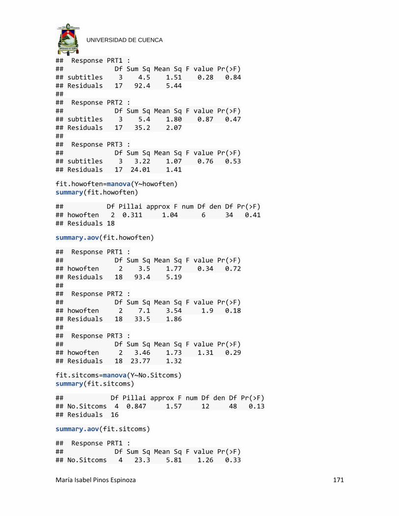
María Isabel Pinos Espinoza 171
UNIVERSIDAD DE CUENCA
## Response PRT1 : ## Df Sum Sq Mean Sq F value Pr(>F) ## subtitles 3 4.5 1.51 0.28 0.84 ## Residuals 17 92.4 5.44 ## ## Response PRT2 : ## Df Sum Sq Mean Sq F value Pr(>F) ## subtitles 3 5.4 1.80 0.87 0.47 ## Residuals 17 35.2 2.07 ## ## Response PRT3 : ## Df Sum Sq Mean Sq F value Pr(>F) ## subtitles 3 3.22 1.07 0.76 0.53 ## Residuals 17 24.01 1.41
fit.howoften=manova(Y~howoften) summary(fit.howoften)
## Df Pillai approx F num Df den Df Pr(>F) ## howoften 2 0.311 1.04 6 34 0.41 ## Residuals 18
summary.aov(fit.howoften)
## Response PRT1 : ## Df Sum Sq Mean Sq F value Pr(>F) ## howoften 2 3.5 1.77 0.34 0.72 ## Residuals 18 93.4 5.19 ## ## Response PRT2 : ## Df Sum Sq Mean Sq F value Pr(>F) ## howoften 2 7.1 3.54 1.9 0.18 ## Residuals 18 33.5 1.86 ## ## Response PRT3 : ## Df Sum Sq Mean Sq F value Pr(>F) ## howoften 2 3.46 1.73 1.31 0.29 ## Residuals 18 23.77 1.32
fit.sitcoms=manova(Y~No.Sitcoms) summary(fit.sitcoms)
## Df Pillai approx F num Df den Df Pr(>F) ## No.Sitcoms 4 0.847 1.57 12 48 0.13 ## Residuals 16
summary.aov(fit.sitcoms)
## Response PRT1 : ## Df Sum Sq Mean Sq F value Pr(>F) ## No.Sitcoms 4 23.3 5.81 1.26 0.33
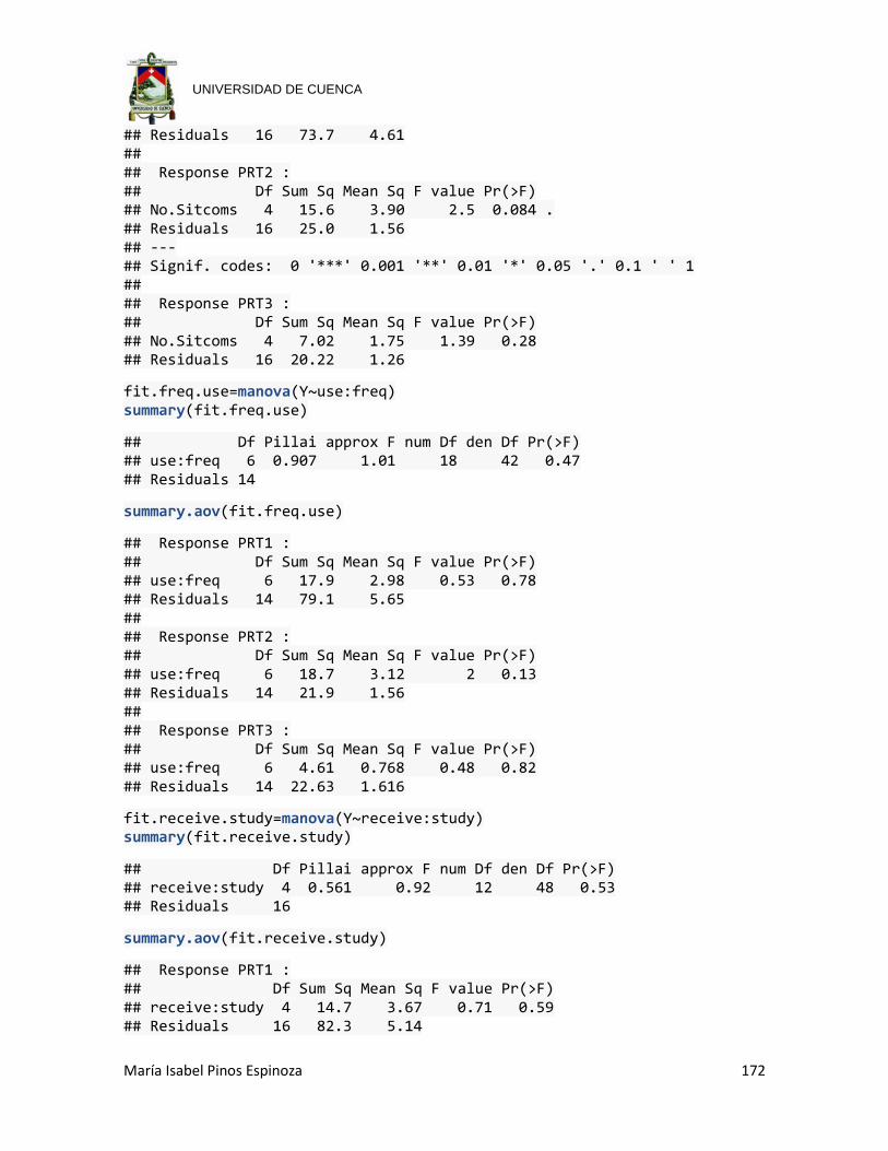
María Isabel Pinos Espinoza 172
UNIVERSIDAD DE CUENCA
## Residuals 16 73.7 4.61 ## ## Response PRT2 : ## Df Sum Sq Mean Sq F value Pr(>F) ## No.Sitcoms 4 15.6 3.90 2.5 0.084 . ## Residuals 16 25.0 1.56 ## --- ## Signif. codes: 0 '***' 0.001 '**' 0.01 '*' 0.05 '.' 0.1 ' ' 1 ## ## Response PRT3 : ## Df Sum Sq Mean Sq F value Pr(>F) ## No.Sitcoms 4 7.02 1.75 1.39 0.28 ## Residuals 16 20.22 1.26
fit.freq.use=manova(Y~use:freq) summary(fit.freq.use)
## Df Pillai approx F num Df den Df Pr(>F) ## use:freq 6 0.907 1.01 18 42 0.47 ## Residuals 14
summary.aov(fit.freq.use)
## Response PRT1 : ## Df Sum Sq Mean Sq F value Pr(>F) ## use:freq 6 17.9 2.98 0.53 0.78 ## Residuals 14 79.1 5.65 ## ## Response PRT2 : ## Df Sum Sq Mean Sq F value Pr(>F) ## use:freq 6 18.7 3.12 2 0.13 ## Residuals 14 21.9 1.56 ## ## Response PRT3 : ## Df Sum Sq Mean Sq F value Pr(>F) ## use:freq 6 4.61 0.768 0.48 0.82 ## Residuals 14 22.63 1.616
fit.receive.study=manova(Y~receive:study) summary(fit.receive.study)
## Df Pillai approx F num Df den Df Pr(>F) ## receive:study 4 0.561 0.92 12 48 0.53 ## Residuals 16
summary.aov(fit.receive.study)
## Response PRT1 : ## Df Sum Sq Mean Sq F value Pr(>F) ## receive:study 4 14.7 3.67 0.71 0.59 ## Residuals 16 82.3 5.14
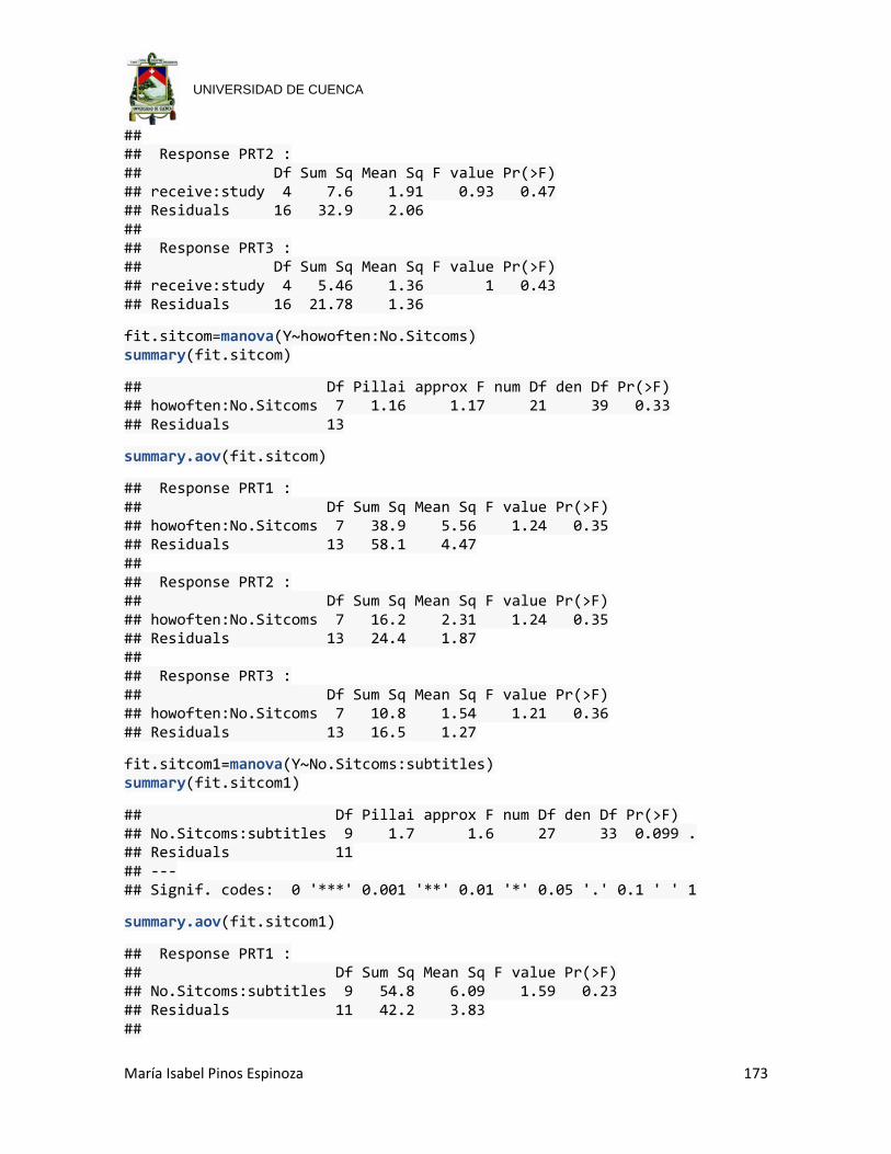
María Isabel Pinos Espinoza 173
UNIVERSIDAD DE CUENCA
## ## Response PRT2 : ## Df Sum Sq Mean Sq F value Pr(>F) ## receive:study 4 7.6 1.91 0.93 0.47 ## Residuals 16 32.9 2.06 ## ## Response PRT3 : ## Df Sum Sq Mean Sq F value Pr(>F) ## receive:study 4 5.46 1.36 1 0.43 ## Residuals 16 21.78 1.36
fit.sitcom=manova(Y~howoften:No.Sitcoms) summary(fit.sitcom)
## Df Pillai approx F num Df den Df Pr(>F) ## howoften:No.Sitcoms 7 1.16 1.17 21 39 0.33 ## Residuals 13
summary.aov(fit.sitcom)
## Response PRT1 : ## Df Sum Sq Mean Sq F value Pr(>F) ## howoften:No.Sitcoms 7 38.9 5.56 1.24 0.35 ## Residuals 13 58.1 4.47 ## ## Response PRT2 : ## Df Sum Sq Mean Sq F value Pr(>F) ## howoften:No.Sitcoms 7 16.2 2.31 1.24 0.35 ## Residuals 13 24.4 1.87 ## ## Response PRT3 : ## Df Sum Sq Mean Sq F value Pr(>F) ## howoften:No.Sitcoms 7 10.8 1.54 1.21 0.36 ## Residuals 13 16.5 1.27
fit.sitcom1=manova(Y~No.Sitcoms:subtitles) summary(fit.sitcom1)
## Df Pillai approx F num Df den Df Pr(>F) ## No.Sitcoms:subtitles 9 1.7 1.6 27 33 0.099 . ## Residuals 11 ## --- ## Signif. codes: 0 '***' 0.001 '**' 0.01 '*' 0.05 '.' 0.1 ' ' 1
summary.aov(fit.sitcom1)
## Response PRT1 : ## Df Sum Sq Mean Sq F value Pr(>F) ## No.Sitcoms:subtitles 9 54.8 6.09 1.59 0.23 ## Residuals 11 42.2 3.83 ##

María Isabel Pinos Espinoza 174
UNIVERSIDAD DE CUENCA
## Response PRT2 : ## Df Sum Sq Mean Sq F value Pr(>F) ## No.Sitcoms:subtitles 9 19.9 2.21 1.18 0.39 ## Residuals 11 20.7 1.88 ## ## Response PRT3 : ## Df Sum Sq Mean Sq F value Pr(>F) ## No.Sitcoms:subtitles 9 16.6 1.84 1.9 0.16 ## Residuals 11 10.7 0.97
fit.sitcom2=manova(Y~watch:No.Sitcoms) summary(fit.sitcom2)
## Df Pillai approx F num Df den Df Pr(>F) ## watch:No.Sitcoms 10 1.56 1.09 30 30 0.41 ## Residuals 10
summary.aov(fit.sitcom2)
## Response PRT1 : ## Df Sum Sq Mean Sq F value Pr(>F) ## watch:No.Sitcoms 10 33.1 3.31 0.52 0.84 ## Residuals 10 63.8 6.38 ## ## Response PRT2 : ## Df Sum Sq Mean Sq F value Pr(>F) ## watch:No.Sitcoms 10 33.8 3.38 5.01 0.0089 ** ## Residuals 10 6.8 0.68 ## --- ## Signif. codes: 0 '***' 0.001 '**' 0.01 '*' 0.05 '.' 0.1 ' ' 1 ## ## Response PRT3 : ## Df Sum Sq Mean Sq F value Pr(>F) ## watch:No.Sitcoms 10 11.2 1.11 0.69 0.71 ## Residuals 10 16.1 1.61
fit.sitcom3=manova(Y~use:watch:No.Sitcoms) summary(fit.sitcom3)
## Df Pillai approx F num Df den Df Pr(>F) ## use:watch:No.Sitcoms 12 1.78 0.973 36 24 0.54 ## Residuals 8
summary.aov(fit.sitcom3)
## Response PRT1 : ## Df Sum Sq Mean Sq F value Pr(>F) ## use:watch:No.Sitcoms 12 47.5 3.95 0.64 0.77 ## Residuals 8 49.5 6.19 ## ## Response PRT2 :
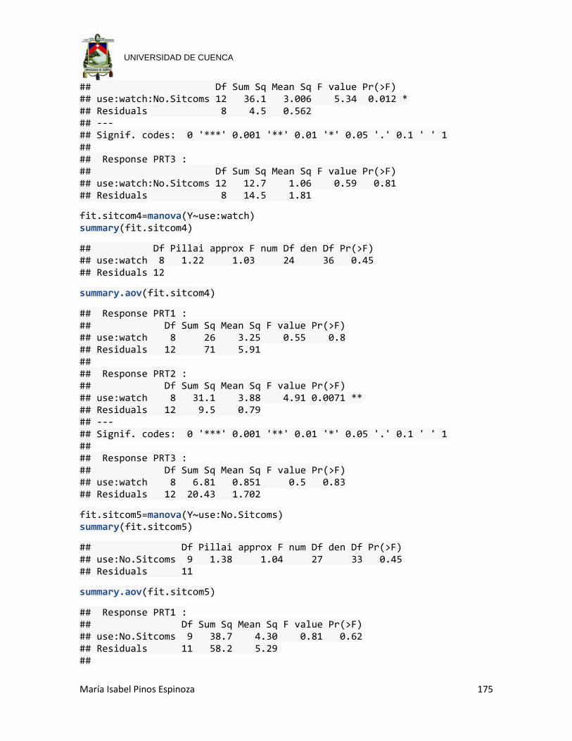
María Isabel Pinos Espinoza 175
UNIVERSIDAD DE CUENCA
## Df Sum Sq Mean Sq F value Pr(>F) ## use:watch:No.Sitcoms 12 36.1 3.006 5.34 0.012 * ## Residuals 8 4.5 0.562 ## --- ## Signif. codes: 0 '***' 0.001 '**' 0.01 '*' 0.05 '.' 0.1 ' ' 1 ## ## Response PRT3 : ## Df Sum Sq Mean Sq F value Pr(>F) ## use:watch:No.Sitcoms 12 12.7 1.06 0.59 0.81 ## Residuals 8 14.5 1.81
fit.sitcom4=manova(Y~use:watch) summary(fit.sitcom4)
## Df Pillai approx F num Df den Df Pr(>F) ## use:watch 8 1.22 1.03 24 36 0.45 ## Residuals 12
summary.aov(fit.sitcom4)
## Response PRT1 : ## Df Sum Sq Mean Sq F value Pr(>F) ## use:watch 8 26 3.25 0.55 0.8 ## Residuals 12 71 5.91 ## ## Response PRT2 : ## Df Sum Sq Mean Sq F value Pr(>F) ## use:watch 8 31.1 3.88 4.91 0.0071 ** ## Residuals 12 9.5 0.79 ## --- ## Signif. codes: 0 '***' 0.001 '**' 0.01 '*' 0.05 '.' 0.1 ' ' 1 ## ## Response PRT3 : ## Df Sum Sq Mean Sq F value Pr(>F) ## use:watch 8 6.81 0.851 0.5 0.83 ## Residuals 12 20.43 1.702
fit.sitcom5=manova(Y~use:No.Sitcoms) summary(fit.sitcom5)
## Df Pillai approx F num Df den Df Pr(>F) ## use:No.Sitcoms 9 1.38 1.04 27 33 0.45 ## Residuals 11
summary.aov(fit.sitcom5)
## Response PRT1 : ## Df Sum Sq Mean Sq F value Pr(>F) ## use:No.Sitcoms 9 38.7 4.30 0.81 0.62 ## Residuals 11 58.2 5.29 ##
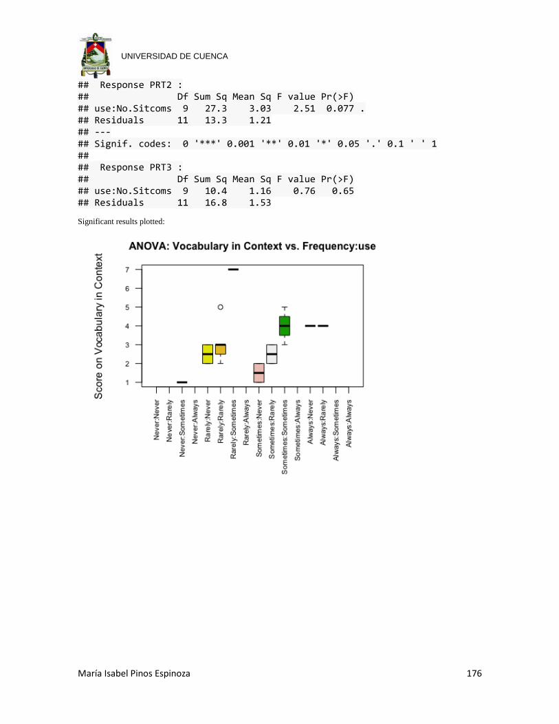
María Isabel Pinos Espinoza 176
UNIVERSIDAD DE CUENCA
## Response PRT2 : ## Df Sum Sq Mean Sq F value Pr(>F) ## use:No.Sitcoms 9 27.3 3.03 2.51 0.077 . ## Residuals 11 13.3 1.21 ## --- ## Signif. codes: 0 '***' 0.001 '**' 0.01 '*' 0.05 '.' 0.1 ' ' 1 ## ## Response PRT3 : ## Df Sum Sq Mean Sq F value Pr(>F) ## use:No.Sitcoms 9 10.4 1.16 0.76 0.65 ## Residuals 11 16.8 1.53
Significant results plotted:
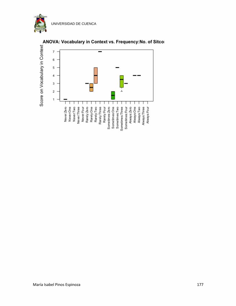
María Isabel Pinos Espinoza 177
UNIVERSIDAD DE CUENCA

María Isabel Pinos Espinoza 178
UNIVERSIDAD DE CUENCA
APPENDIX 12 MULTIVARIATE ANALYSIS OF VARIANCE OF ALL PARTICIPANTS RESULTS ACCORDING TO TEACHER-DEFINED LEVEL WITH ADVANCED PARTICIPANT AND THE PARTICIPANTS REMOVED FROM THE MANOVAS OF BEGINNERS AND INTERMEDIATES REMOVED.
Key:
study = Hours participants study English throughout the week No.Sitcoms = No. Sitcoms watched by participants (Derived Variable) use = Frequency participants use English with friends or family receive = Frequency participants receive private English classes subtitles = Whether participants use English or Spanish subtitles watch = Frequency participants watch English language Sitcoms howoften = how many times participants watched sitcoms the previous week freq = Frequency with which participants are in contact with English outside the classroom. PRT1 = Score on the Vocabulary section of the pretest PRT2 = Score on the Vocabulary in Context section of the pretest PRT3 = Score on the Reading Comprehension section of the pretest Y = Table with PRT1, PRT2, and PRT3
fit.age=manova(Y~age) summary(fit.age)
## Df Pillai approx F num Df den Df Pr(>F) ## age 3 0.257 0.469 9 45 0.89 ## Residuals 15
summary.aov(fit.age)
## Response PRT1 : ## Df Sum Sq Mean Sq F value Pr(>F) ## age 3 11.5 3.83 0.72 0.55 ## Residuals 15 79.7 5.31 ## ## Response PRT2 : ## Df Sum Sq Mean Sq F value Pr(>F) ## age 3 2.1 0.70 0.31 0.82 ## Residuals 15 33.6 2.24 ## ## Response PRT3 : ## Df Sum Sq Mean Sq F value Pr(>F) ## age 3 2.87 0.958 0.63 0.61 ## Residuals 15 22.92 1.528
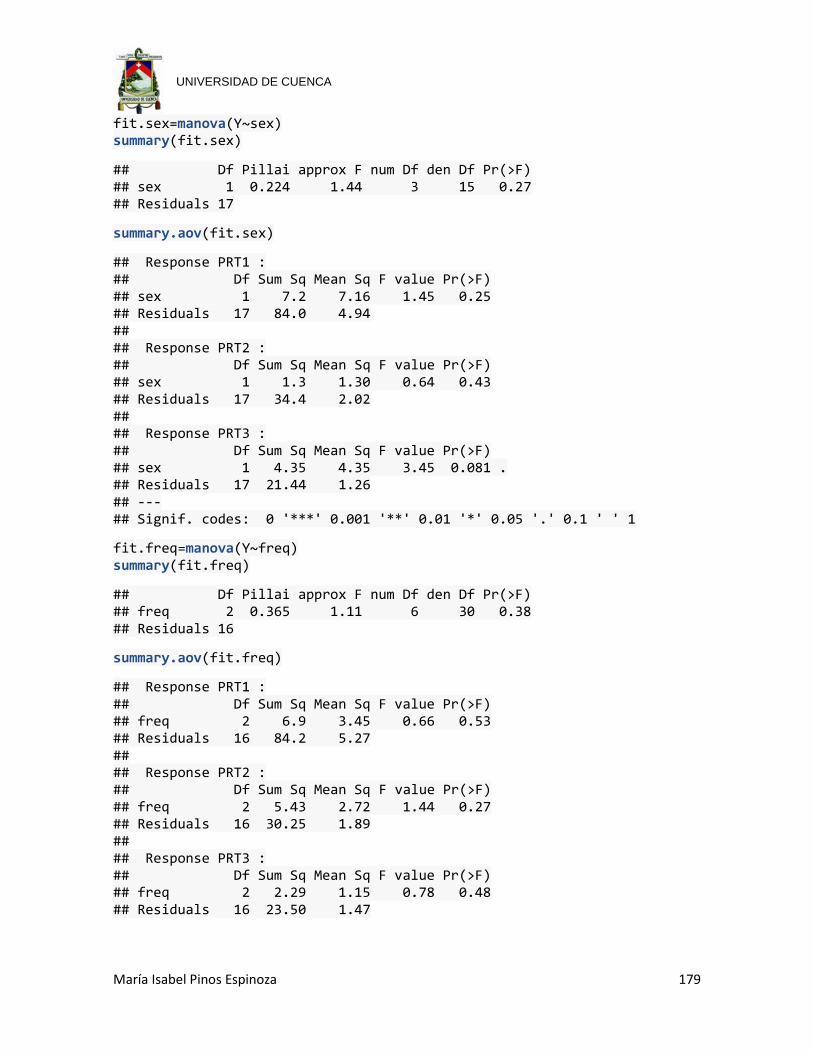
María Isabel Pinos Espinoza 179
UNIVERSIDAD DE CUENCA
fit.sex=manova(Y~sex) summary(fit.sex)
## Df Pillai approx F num Df den Df Pr(>F) ## sex 1 0.224 1.44 3 15 0.27 ## Residuals 17
summary.aov(fit.sex)
## Response PRT1 : ## Df Sum Sq Mean Sq F value Pr(>F) ## sex 1 7.2 7.16 1.45 0.25 ## Residuals 17 84.0 4.94 ## ## Response PRT2 : ## Df Sum Sq Mean Sq F value Pr(>F) ## sex 1 1.3 1.30 0.64 0.43 ## Residuals 17 34.4 2.02 ## ## Response PRT3 : ## Df Sum Sq Mean Sq F value Pr(>F) ## sex 1 4.35 4.35 3.45 0.081 . ## Residuals 17 21.44 1.26 ## --- ## Signif. codes: 0 '***' 0.001 '**' 0.01 '*' 0.05 '.' 0.1 ' ' 1
fit.freq=manova(Y~freq) summary(fit.freq)
## Df Pillai approx F num Df den Df Pr(>F) ## freq 2 0.365 1.11 6 30 0.38 ## Residuals 16
summary.aov(fit.freq)
## Response PRT1 : ## Df Sum Sq Mean Sq F value Pr(>F) ## freq 2 6.9 3.45 0.66 0.53 ## Residuals 16 84.2 5.27 ## ## Response PRT2 : ## Df Sum Sq Mean Sq F value Pr(>F) ## freq 2 5.43 2.72 1.44 0.27 ## Residuals 16 30.25 1.89 ## ## Response PRT3 : ## Df Sum Sq Mean Sq F value Pr(>F) ## freq 2 2.29 1.15 0.78 0.48 ## Residuals 16 23.50 1.47
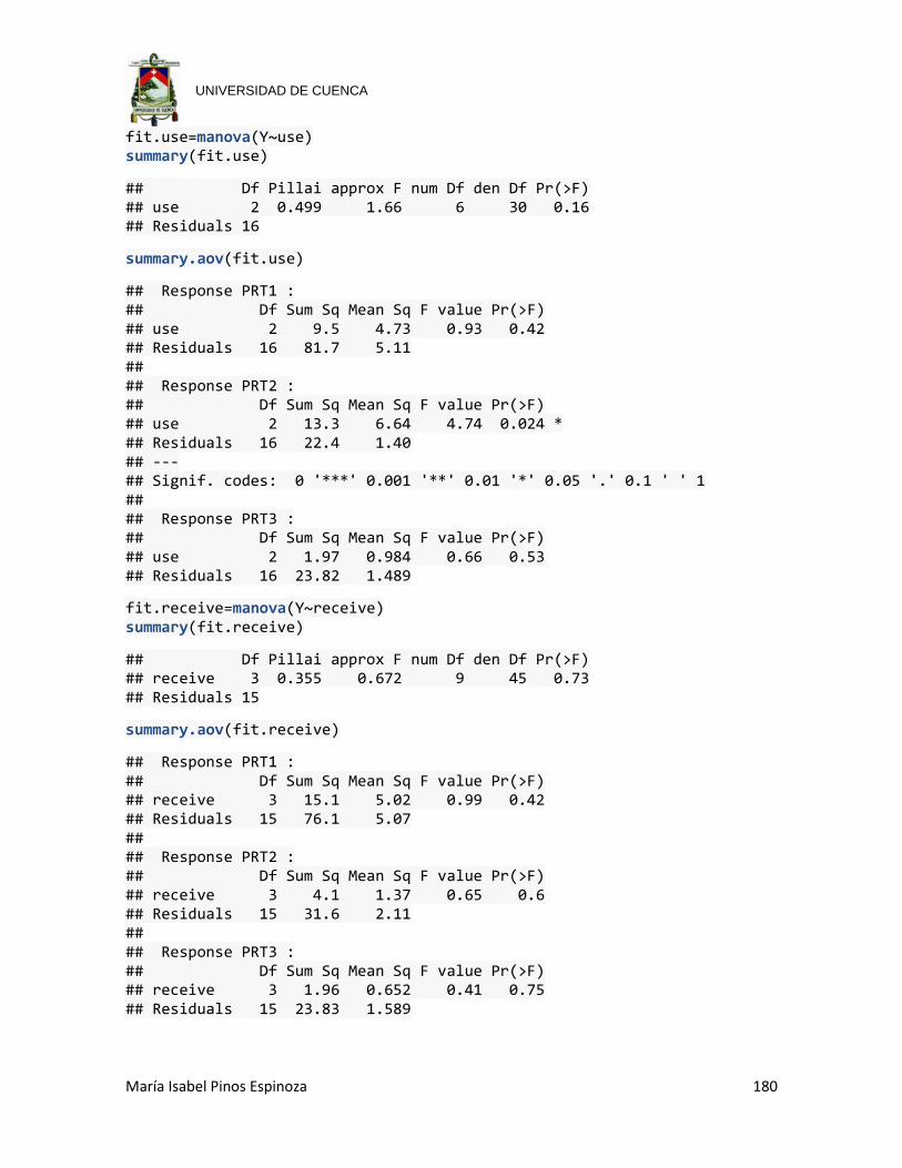
María Isabel Pinos Espinoza 180
UNIVERSIDAD DE CUENCA
fit.use=manova(Y~use) summary(fit.use)
## Df Pillai approx F num Df den Df Pr(>F) ## use 2 0.499 1.66 6 30 0.16 ## Residuals 16
summary.aov(fit.use)
## Response PRT1 : ## Df Sum Sq Mean Sq F value Pr(>F) ## use 2 9.5 4.73 0.93 0.42 ## Residuals 16 81.7 5.11 ## ## Response PRT2 : ## Df Sum Sq Mean Sq F value Pr(>F) ## use 2 13.3 6.64 4.74 0.024 * ## Residuals 16 22.4 1.40 ## --- ## Signif. codes: 0 '***' 0.001 '**' 0.01 '*' 0.05 '.' 0.1 ' ' 1 ## ## Response PRT3 : ## Df Sum Sq Mean Sq F value Pr(>F) ## use 2 1.97 0.984 0.66 0.53 ## Residuals 16 23.82 1.489
fit.receive=manova(Y~receive) summary(fit.receive)
## Df Pillai approx F num Df den Df Pr(>F) ## receive 3 0.355 0.672 9 45 0.73 ## Residuals 15
summary.aov(fit.receive)
## Response PRT1 : ## Df Sum Sq Mean Sq F value Pr(>F) ## receive 3 15.1 5.02 0.99 0.42 ## Residuals 15 76.1 5.07 ## ## Response PRT2 : ## Df Sum Sq Mean Sq F value Pr(>F) ## receive 3 4.1 1.37 0.65 0.6 ## Residuals 15 31.6 2.11 ## ## Response PRT3 : ## Df Sum Sq Mean Sq F value Pr(>F) ## receive 3 1.96 0.652 0.41 0.75 ## Residuals 15 23.83 1.589

María Isabel Pinos Espinoza 181
UNIVERSIDAD DE CUENCA
fit.study=manova(Y~study) summary(fit.study)
## Df Pillai approx F num Df den Df Pr(>F) ## study 1 0.102 0.565 3 15 0.65 ## Residuals 17
summary.aov(fit.study)
## Response PRT1 : ## Df Sum Sq Mean Sq F value Pr(>F) ## study 1 2.7 2.7 0.52 0.48 ## Residuals 17 88.5 5.2 ## ## Response PRT2 : ## Df Sum Sq Mean Sq F value Pr(>F) ## study 1 0.5 0.481 0.23 0.64 ## Residuals 17 35.2 2.071 ## ## Response PRT3 : ## Df Sum Sq Mean Sq F value Pr(>F) ## study 1 0.39 0.388 0.26 0.62 ## Residuals 17 25.40 1.494
fit.watch=manova(Y~watch) summary(fit.watch)
## Df Pillai approx F num Df den Df Pr(>F) ## watch 2 0.218 0.612 6 30 0.72 ## Residuals 16
summary.aov(fit.watch)
## Response PRT1 : ## Df Sum Sq Mean Sq F value Pr(>F) ## watch 2 6.6 3.28 0.62 0.55 ## Residuals 16 84.6 5.29 ## ## Response PRT2 : ## Df Sum Sq Mean Sq F value Pr(>F) ## watch 2 1.7 0.842 0.4 0.68 ## Residuals 16 34.0 2.125 ## ## Response PRT3 : ## Df Sum Sq Mean Sq F value Pr(>F) ## watch 2 3.57 1.78 1.28 0.3 ## Residuals 16 22.22 1.39
fit.subtitles=manova(Y~subtitles) summary(fit.subtitles)

María Isabel Pinos Espinoza 182
UNIVERSIDAD DE CUENCA
## Df Pillai approx F num Df den Df Pr(>F) ## subtitles 2 0.157 0.426 6 30 0.86 ## Residuals 16
summary.aov(fit.subtitles)
## Response PRT1 : ## Df Sum Sq Mean Sq F value Pr(>F) ## subtitles 2 4.7 2.36 0.44 0.65 ## Residuals 16 86.4 5.40 ## ## Response PRT2 : ## Df Sum Sq Mean Sq F value Pr(>F) ## subtitles 2 0.6 0.288 0.13 0.88 ## Residuals 16 35.1 2.194 ## ## Response PRT3 : ## Df Sum Sq Mean Sq F value Pr(>F) ## subtitles 2 2.22 1.11 0.75 0.49 ## Residuals 16 23.57 1.47
fit.howoften=manova(Y~howoften) summary(fit.howoften)
## Df Pillai approx F num Df den Df Pr(>F) ## howoften 2 0.325 0.97 6 30 0.46 ## Residuals 16
summary.aov(fit.howoften)
## Response PRT1 : ## Df Sum Sq Mean Sq F value Pr(>F) ## howoften 2 18.5 9.25 2.04 0.16 ## Residuals 16 72.7 4.54 ## ## Response PRT2 : ## Df Sum Sq Mean Sq F value Pr(>F) ## howoften 2 4.18 2.09 1.06 0.37 ## Residuals 16 31.50 1.97 ## ## Response PRT3 : ## Df Sum Sq Mean Sq F value Pr(>F) ## howoften 2 2.27 1.13 0.77 0.48 ## Residuals 16 23.52 1.47
fit.sitcoms=manova(Y~No.Sitcoms) summary(fit.sitcoms)
## Df Pillai approx F num Df den Df Pr(>F) ## No.Sitcoms 3 0.664 1.42 9 45 0.21 ## Residuals 15
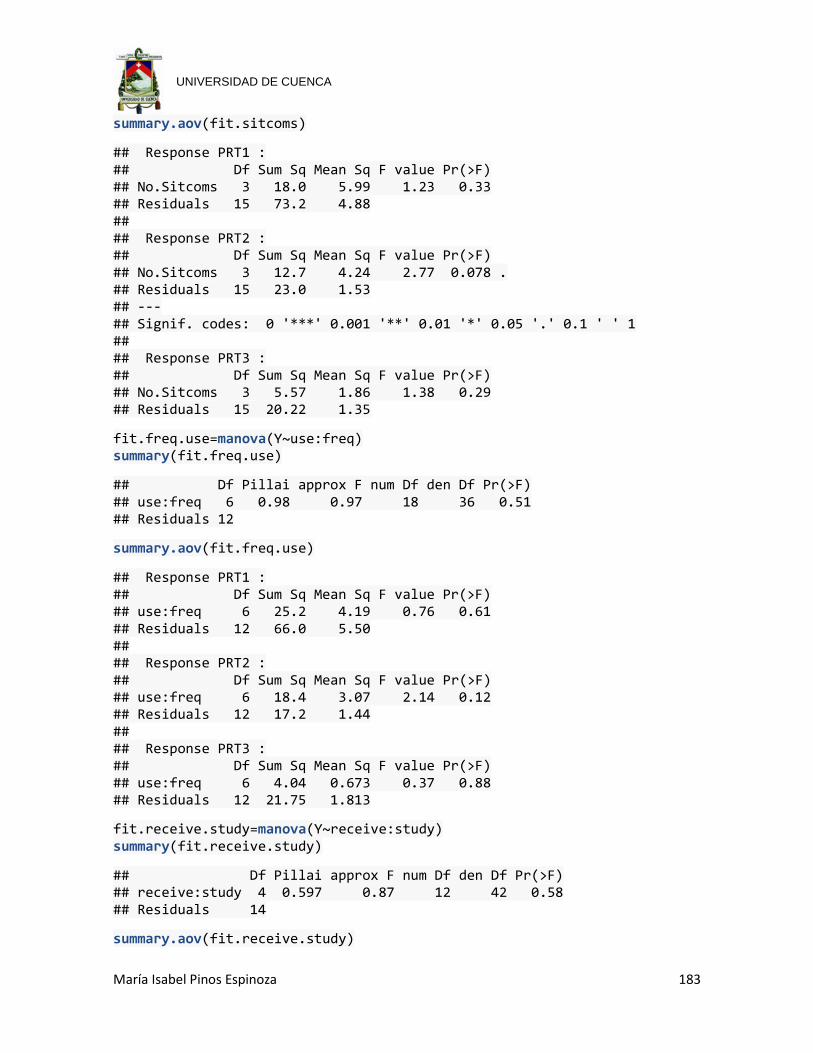
María Isabel Pinos Espinoza 183
UNIVERSIDAD DE CUENCA
summary.aov(fit.sitcoms)
## Response PRT1 : ## Df Sum Sq Mean Sq F value Pr(>F) ## No.Sitcoms 3 18.0 5.99 1.23 0.33 ## Residuals 15 73.2 4.88 ## ## Response PRT2 : ## Df Sum Sq Mean Sq F value Pr(>F) ## No.Sitcoms 3 12.7 4.24 2.77 0.078 . ## Residuals 15 23.0 1.53 ## --- ## Signif. codes: 0 '***' 0.001 '**' 0.01 '*' 0.05 '.' 0.1 ' ' 1 ## ## Response PRT3 : ## Df Sum Sq Mean Sq F value Pr(>F) ## No.Sitcoms 3 5.57 1.86 1.38 0.29 ## Residuals 15 20.22 1.35
fit.freq.use=manova(Y~use:freq) summary(fit.freq.use)
## Df Pillai approx F num Df den Df Pr(>F) ## use:freq 6 0.98 0.97 18 36 0.51 ## Residuals 12
summary.aov(fit.freq.use)
## Response PRT1 : ## Df Sum Sq Mean Sq F value Pr(>F) ## use:freq 6 25.2 4.19 0.76 0.61 ## Residuals 12 66.0 5.50 ## ## Response PRT2 : ## Df Sum Sq Mean Sq F value Pr(>F) ## use:freq 6 18.4 3.07 2.14 0.12 ## Residuals 12 17.2 1.44 ## ## Response PRT3 : ## Df Sum Sq Mean Sq F value Pr(>F) ## use:freq 6 4.04 0.673 0.37 0.88 ## Residuals 12 21.75 1.813
fit.receive.study=manova(Y~receive:study) summary(fit.receive.study)
## Df Pillai approx F num Df den Df Pr(>F) ## receive:study 4 0.597 0.87 12 42 0.58 ## Residuals 14
summary.aov(fit.receive.study)
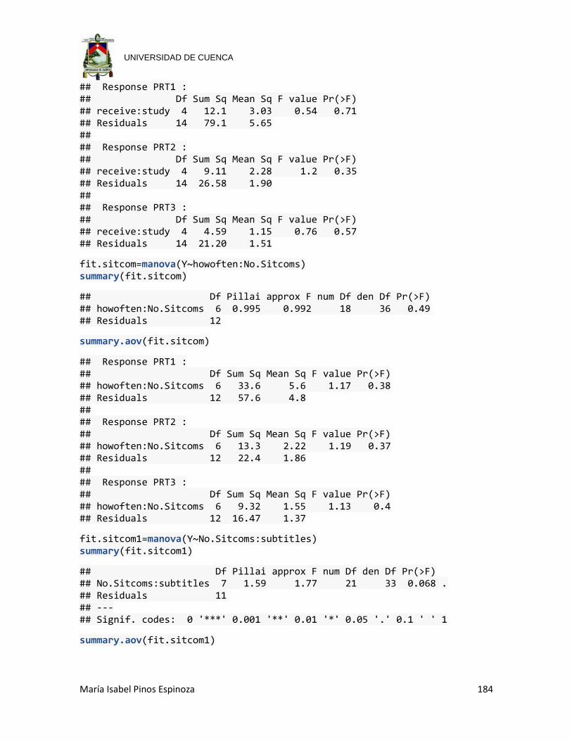
María Isabel Pinos Espinoza 184
UNIVERSIDAD DE CUENCA
## Response PRT1 : ## Df Sum Sq Mean Sq F value Pr(>F) ## receive:study 4 12.1 3.03 0.54 0.71 ## Residuals 14 79.1 5.65 ## ## Response PRT2 : ## Df Sum Sq Mean Sq F value Pr(>F) ## receive:study 4 9.11 2.28 1.2 0.35 ## Residuals 14 26.58 1.90 ## ## Response PRT3 : ## Df Sum Sq Mean Sq F value Pr(>F) ## receive:study 4 4.59 1.15 0.76 0.57 ## Residuals 14 21.20 1.51
fit.sitcom=manova(Y~howoften:No.Sitcoms) summary(fit.sitcom)
## Df Pillai approx F num Df den Df Pr(>F) ## howoften:No.Sitcoms 6 0.995 0.992 18 36 0.49 ## Residuals 12
summary.aov(fit.sitcom)
## Response PRT1 : ## Df Sum Sq Mean Sq F value Pr(>F) ## howoften:No.Sitcoms 6 33.6 5.6 1.17 0.38 ## Residuals 12 57.6 4.8 ## ## Response PRT2 : ## Df Sum Sq Mean Sq F value Pr(>F) ## howoften:No.Sitcoms 6 13.3 2.22 1.19 0.37 ## Residuals 12 22.4 1.86 ## ## Response PRT3 : ## Df Sum Sq Mean Sq F value Pr(>F) ## howoften:No.Sitcoms 6 9.32 1.55 1.13 0.4 ## Residuals 12 16.47 1.37
fit.sitcom1=manova(Y~No.Sitcoms:subtitles) summary(fit.sitcom1)
## Df Pillai approx F num Df den Df Pr(>F) ## No.Sitcoms:subtitles 7 1.59 1.77 21 33 0.068 . ## Residuals 11 ## --- ## Signif. codes: 0 '***' 0.001 '**' 0.01 '*' 0.05 '.' 0.1 ' ' 1
summary.aov(fit.sitcom1)

María Isabel Pinos Espinoza 185
UNIVERSIDAD DE CUENCA
## Response PRT1 : ## Df Sum Sq Mean Sq F value Pr(>F) ## No.Sitcoms:subtitles 7 49.0 7.00 1.83 0.18 ## Residuals 11 42.2 3.83 ## ## Response PRT2 : ## Df Sum Sq Mean Sq F value Pr(>F) ## No.Sitcoms:subtitles 7 15.0 2.15 1.14 0.4 ## Residuals 11 20.7 1.88 ## ## Response PRT3 : ## Df Sum Sq Mean Sq F value Pr(>F) ## No.Sitcoms:subtitles 7 15.1 2.16 2.23 0.11 ## Residuals 11 10.7 0.97
fit.sitcom2=manova(Y~watch:No.Sitcoms) summary(fit.sitcom2)
## Df Pillai approx F num Df den Df Pr(>F) ## watch:No.Sitcoms 8 1.39 1.08 24 30 0.42 ## Residuals 10
summary.aov(fit.sitcom2)
## Response PRT1 : ## Df Sum Sq Mean Sq F value Pr(>F) ## watch:No.Sitcoms 8 27.3 3.42 0.54 0.81 ## Residuals 10 63.8 6.38 ## ## Response PRT2 : ## Df Sum Sq Mean Sq F value Pr(>F) ## watch:No.Sitcoms 8 28.93 3.62 5.36 0.0081 ** ## Residuals 10 6.75 0.68 ## --- ## Signif. codes: 0 '***' 0.001 '**' 0.01 '*' 0.05 '.' 0.1 ' ' 1 ## ## Response PRT3 : ## Df Sum Sq Mean Sq F value Pr(>F) ## watch:No.Sitcoms 8 9.71 1.21 0.75 0.65 ## Residuals 10 16.08 1.61
fit.sitcom3=manova(Y~use:watch:No.Sitcoms) summary(fit.sitcom3)
## Df Pillai approx F num Df den Df Pr(>F) ## use:watch:No.Sitcoms 10 1.61 0.931 30 24 0.58 ## Residuals 8
summary.aov(fit.sitcom3)

María Isabel Pinos Espinoza 186
UNIVERSIDAD DE CUENCA
## Response PRT1 : ## Df Sum Sq Mean Sq F value Pr(>F) ## use:watch:No.Sitcoms 10 41.7 4.17 0.67 0.73 ## Residuals 8 49.5 6.19 ## ## Response PRT2 : ## Df Sum Sq Mean Sq F value Pr(>F) ## use:watch:No.Sitcoms 10 31.2 3.118 5.54 0.012 * ## Residuals 8 4.5 0.563 ## --- ## Signif. codes: 0 '***' 0.001 '**' 0.01 '*' 0.05 '.' 0.1 ' ' 1 ## ## Response PRT3 : ## Df Sum Sq Mean Sq F value Pr(>F) ## use:watch:No.Sitcoms 10 11.3 1.13 0.62 0.76 ## Residuals 8 14.5 1.81
fit.sitcom4=manova(Y~use:watch) summary(fit.sitcom4)
## Df Pillai approx F num Df den Df Pr(>F) ## use:watch 7 1.11 0.925 21 33 0.57 ## Residuals 11
summary.aov(fit.sitcom4)
## Response PRT1 : ## Df Sum Sq Mean Sq F value Pr(>F) ## use:watch 7 27.9 3.99 0.69 0.68 ## Residuals 11 63.2 5.75 ## ## Response PRT2 : ## Df Sum Sq Mean Sq F value Pr(>F) ## use:watch 7 26.2 3.74 4.33 0.015 * ## Residuals 11 9.5 0.86 ## --- ## Signif. codes: 0 '***' 0.001 '**' 0.01 '*' 0.05 '.' 0.1 ' ' 1 ## ## Response PRT3 : ## Df Sum Sq Mean Sq F value Pr(>F) ## use:watch 7 5.46 0.779 0.42 0.87 ## Residuals 11 20.33 1.848
fit.sitcom5=manova(Y~use:No.Sitcoms) summary(fit.sitcom5)
## Df Pillai approx F num Df den Df Pr(>F) ## use:No.Sitcoms 7 1.17 1 21 33 0.48 ## Residuals 11
summary.aov(fit.sitcom5)

María Isabel Pinos Espinoza 187
UNIVERSIDAD DE CUENCA
## Response PRT1 : ## Df Sum Sq Mean Sq F value Pr(>F) ## use:No.Sitcoms 7 32.9 4.71 0.89 0.55 ## Residuals 11 58.2 5.29 ## ## Response PRT2 : ## Df Sum Sq Mean Sq F value Pr(>F) ## use:No.Sitcoms 7 22.4 3.20 2.64 0.072 . ## Residuals 11 13.3 1.21 ## --- ## Signif. codes: 0 '***' 0.001 '**' 0.01 '*' 0.05 '.' 0.1 ' ' 1 ## ## Response PRT3 : ## Df Sum Sq Mean Sq F value Pr(>F) ## use:No.Sitcoms 7 8.99 1.28 0.84 0.58 ## Residuals 11 16.80 1.53
Significant results plotted:
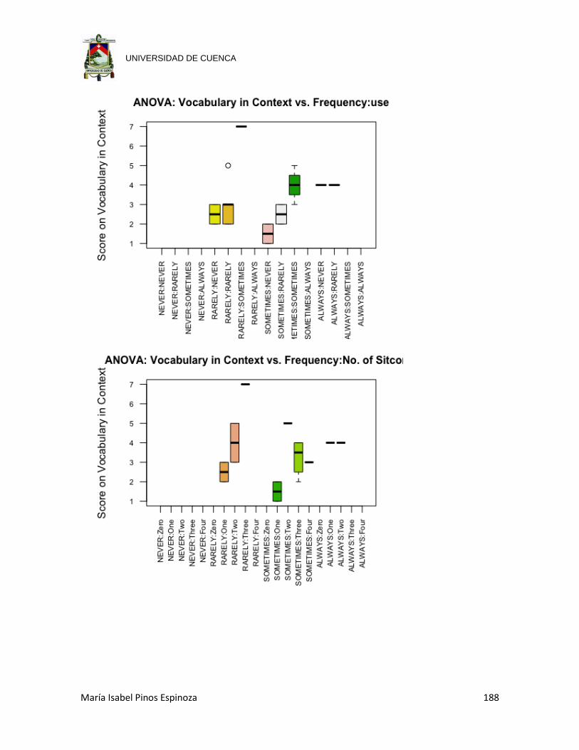
María Isabel Pinos Espinoza 188
UNIVERSIDAD DE CUENCA