UNIVERSIDAD DE ALICANTE FACULTAD DE CIENCIAS ECONÓMICAS … · UNIVERSIDAD DE ALICANTE FACULTAD DE...

UNIVERSIDAD DE ALICANTE

FACULTAD DE CIENCIAS ECONÓMICAS Y EMPRESARIALES

GRADO EN ECONOMÍA

CURSO ACADÉMICO 2016 - 2017

Gender wage gap. A complete view from Italy

Autor: Miguel Angel González Simón

Tutor: Francesco Serti

Investigación en econometría aplicada

Alicante, Julio de 2017

2

Abstract

Wage discrimination has been widely investigated so that I try to contribute to this

strand of the literature showing if there is evidence to exist in Italy for the period from

2000 to 2012 by using panel data from SHIW. Moreover, I focus the investigation on

the informal labour market but I also do on the formal one. To get this, I perform

Oaxaca-Blinder decomposition model. The main goal of these estimates is observing

whether the results change when I include a variable to control non-random selection

processes. In accordance with this, I obtain that gender wage gap is larger among formal

workers when I control for this correction term than when I do not control for it and

smaller among informal workers. Finally, I perform a robustness check to observe how

this discrimination affects in each part of the informal workers distribution.

Keywords: wage discrimination, informal labour market, Italy, non-random selection

3

Index

1. Introduction and literature review……………………………4

2. Data collection………………………………………………….8

3. Empirical strategy…………………………………………......9

The raw and adjusted wage gaps………………9

Treatment for selection into multiple statuses.11

Identification…………………………………….14

4. Descriptive statistics…………………………………………15

5. Results…………………………………………………………21

6. Robustness checks…………………………………………..26

7. Conclusions…………………………………………………..28

8. References……………………………………………………30

9. Appendix……………………………………………………..31

4

1. Introduction and literature review

Shadow economy plays a role in the GDP of all the countries of the world although the

size of this is different for each other. Recent estimates indicate that the undeclared

sector represents a lower value for developed countries than for developing countries. In

particular, Enste (2015) finds that german and italian shadow economies indicate 14.6%

and 22.5% of GDP in the period 2003-2013, respectively meanwhile for countries such

as Panama or Bolivia Schneider (2007) shows that it becomes almost 70% of GDP.

About the shadow economy behaviour, there is strong evidence to state that the size of

it is counter-cyclical, that is, the size of the shadow economy as a ratio of GDP is bigger

in bad bussiness cycles and is reduced in good ones (Elgin, 2012).

Regarding selections processes, there is evidence that the individuals follow non-

random selection into jobs, meaning that formal workers are systematically different

from informal workers in a way that affect their wages even after controlling for

observable characteristics. Looking at European countries and the United States,

Olivetti and Petrongolo (2008) point out that non-random selection explains why gender

employment gaps are negatively correlated with gender wage gaps accross countries.

Since I consider that there is three possible statuses: unemployed, formal worker and

informal one, I follow the Bourguignon, Fournier and Gurgand (2004) method by

adding a correction term with I control for the non-random selection processes of

staying either in a status or in another. According to the related literature, some

investigators consider just two statuses and they follow the methodology proposed by

Heckman (1973) (Tansel, 2001; Deininger et al., 2013) to control for selection.

In order to perform a study about this topic we need reliable data but this is not always

possible because people who are interviewed could think that they have been

investigated and they may not tell the truth in their answers. However, in the last years

there have been some advances in this field by performing randomized experiments

(Kleven et al., 2011) or by trying to solve the selection problem (Di Porto, 2011; Di

Porto et al., 2013).

Regarding Italian shadow economy its size is around 22.5% of GDP as I mentioned

above and is a country where there have been established some policies against it. An

5

example of these may be the Biagi reform with a focus on the objectives of the

European Employment Strategy.

This reform was enacted by Legislative Decree No. 276/2003 and it aimed to raise

employment levels, promote labour market access for disadvantaged groups and

increase the number of workers in stable employment. It led to an increase in the level

of this last goal but a proper assessment will only be posible in a longer time frame

(Tiraboschi, 2005).

In this sense, Di Porto and Elia, 2013 use an identification strategy based on three

amnesty laws and they suggest that all of them changed the shape of the undeclared

sector in Italy causing a rapid emergence from this sector to the formal one. According

to this statement, (Di Porto et al., 2013) performed an investigation to check if this

effect was caused by these laws and they do not find a clear result.

A possible problem related with the ineffectivenss of labour policies is that there is

evidence to state that there is no connection between formal and informal sectors what

supports the failure to transform black employment into regular one over the last twenty

years (Bovi, 2005).

Moreover, some investigators study the effect of the size of the undeclared sector on

other labour market outcomes such as financial development (Capasso Jappelli, 2013)

and they obtain that the local financial development is associated with a smaller size of

the underground economy.

Focusing on how the undeclared sector structure is related with the level of education of

workers, Cappariello and Zizza in 2010 conclude that the probability to end up working

in this sector is higher for those who have performed fewer years of education. These

results are based on the same data we use but for different years and they also suggest

that the wages are slightly higher for individuals who performed the compulsory

education with respect to those who did not in the informal sector.

If we refer to Italy’s economy is worth mentioning the role of immigrants because it is a

country characterized by receiving people from abroad in last recent decades. Moreover,

this immigration has been chaotic because most of them are from individuals who run

away from their origin countries.

6

Therefore, how they are integrated in the labour market is interesting and, in this sense,

there is evidence to their jobs are full of irregular components, but difficult to divide

from the functioning of the official economy and the host society (Ambrosini, 2001).

This paper is related to the literature on the dualistic view of the labour market and

according to this view, the informal labour market is characterized by lower wages so

that this paper presents some evidence to explain that the formal gender wage gap

differs from the informal one.

Therefore, if we look at the female labour market history, we may observe that they

have been rejected for several reasons until some decades ago, when they were able to

enter the labour market after several fights. Despite having the possibility to get a job,

there has always been evidence of wage discrimination as Hegewisch and Williams

(2010) suggest.

In the last years governments from many countries have performed policies to reduce

the discrimination although it is still persistent and pronounced between male and

female in all the parts of the world (Hirsch, 2016).

In spite of this Oostendorp, R., 2009 studied the relationship between the economic

development and the occupational gender wage gap in richer countries and he suggests

that the gap tends to decrease with increasing economic development in these countries.

We may think that this discrimination is provoked by the different education level

achieved by individuals because it is likely that women have not the same opportunities

to study than men. However, Livanos and Núñez (2012) study the effect of the

education level on the unexplained part of the wage gap, which is often related to

discrimination, and they find that it is lower for graduates in Greece and UK.

In addition, Arhsad and Ghani (2015) also studied whether there exists the gap for the

same education level and they suggest that in Malaysia male wages are much higher

than female ones within each education group.

For Spain, de la Rica et al. (2008) also find that the gender wage gap is high and

increases with the wage among highly educated workers while it is lower and decreases

with wage among less educated workers.

7

We may also think that a way to reduce the gap is applying policies with the aim to

increase the occupational integration because there is evidence that occupational

segregation is strongly correlated with gender earnings inequality, as suggest Cotter and

DeFiore, 1997.

If we look at Italy, Mussida and Picchio, 2014 used data for the last two decades and

they find that the unconditional gender wage gap remained roughly constant over time,

however, they also suggest that the component of the gap due to different rewards of

similar characteristics deteriorated women’s relative wage.

Moreover, these authors, by using microdata from Italy for the formal labour market,

found that those women who had a lower education level are really penalized in their

salaries (Mussida and Picchio, 2012).

Finally, focusing on papers which investigate gender wage gap in the undeclared sector

we just find (Yahmed, 2016) where it is used data from Brazil and she finds that gender

wage gap is higher in the informal labour market than in the formal one but she also

argues that this may be provoked by the selection processes which determines why

individuals choose either a sector or another. This is why she controls for endogenous

selection into both sectors and we will try to do the same.

The remainder part is organized as follows. The Section 2 explains what data I use to

estimate the model and how I obtained it and the Section 3 is about the empirical

strategy I follow where I explain with detail why I perform each step. The next section

shows the descriptive statistics and the fifth one presents the main results of the model.

The last two sections are added to show some robustness checks and the conclusions.

8

2. Data collection

To perform the empirical analysis I use individual data from the Bank of Italy – Survey

on Household Income and Wealth (SHIW). This dataset shows a highly detailed

information from different perspectives by using some multipurpose surveys where we

may observe distributional information and evidence on correlations such as family

composition with economic behaviour. This is really important because it allows us to

observe the effect through different subpopulations and to establish causality from a

policy. The survey is carried out every two years and to the scope of this paper I

consider the period 2000-2012. The target population includes individuals aged from 15

to 65 and amounts to 96299 observations. I restrict the sample to this range because

these are the legal years to work according to italian laws. It also provides information

on demographic characteristics, household composition, specifications related to the

job, and standard labour market outcomes. To identify the experience of the individuals

I consider the potential experience variable presented by substracting the age the

individual is at contemporary moment and the age when he/she started to work. This

way to calculate the potential experience presents some problems because it does not

take into account those periods when the individual is not active in the labour market

such as when he/she is unemployed. Regarding earnings, I compute them as the ratio

between nominal earnings and the inflation rate using monthly values, because using

salaries per hour may present some problems as I have to assume the number of weeks

individuals work per month. I calculate wages this way to be able to compare them for

all workers. Taking into account all of this, the definition I use to identify informal

workers is considering those who have positive wages without receiving paid social

security contributions throughout his working career. The latter information is obtained,

as some investigators who use this survey (Di Porto Elia, 2013; Cappariello Zizza,

2010), with the following question: Considering the employment history of. . . (name),

did he/she ever pay, or his/her employer pay, the social security contributions even for

a short period? so that, if the individual gives a negative reply, along with a positive

wage, there is evidence that he/she worked in the informal labour market (Di Porto,

2015). In addition, I generate another definition of informal worker by calculating a

ratio between the same question I use above and the potential experience, although I just

use this as robustness check. However, this definition may present some misreporting

values since individuals may not say the truth about the earnings for fear of being

9

detected by the authorities, although I can exclude this possibility because the survey is

anonimous. Moreover, to avoid problems about the tax calculation to obtain the net

wages, I should use gross ones but it is not possible because they are not available and,

therefore, it may lead to not too accurate results. Finally, due to labour market decisions

and observed gender wage gaps differ accross the schooling distribution, I construct a

regional unemployment rate for different education groups in order to identify the

impact of lower labour demand even when controlling for regional dummies.

3. Estimation Strategy

As I mentioned across all the paper I replicate the model proposed in Yahmed (2016)

with data from Italy, this will may be useful in two ways: the first one is upon the

results she obtains in her investigation because if I get similar ones there is evidence

that the model may be correctly specified and the second reason is that I may be able to

contribute into this part of literature by performing some robustness checks and

checking if this gap also exists when it is used different proxies of informal workers and

using different subpopulations as I do in the final section of the paper.

In order to estimate the gender wage gap in the informal labor market and in the formal

one I explain in this section the model I use where I first estimate the raw and adjusted

wages by controlling for observable characteristics and then, I also control for selection

into the different labour statuses.

3.1 The raw and adjusted wage gaps

This section shows some simple ways to obtain gender wage gap only controlling for

observable characteristics. To do this I present how to calculate the raw wage gap and

the adjusted wage one.

The first simple idea we could perform to obtain the raw wage gap in the different

sectors from a simple equation:

ln(𝑤𝑖𝑗) = 𝛽0 + 𝛼𝑗 ∗ 𝐹𝑖𝑗 + 𝑢𝑖𝑗 (1)

10

where the dependent variable is the log wage and F is a dummy equal to one when

indicates if the employee i is a woman and the sub-index j shows the sector where the

individual belongs.

In this equation, I am interested in the coefficient we obtain (𝛼𝑗) because it indicates the

wage difference between male and female individuals1. However, this equation may

present some important problems. One of them is that it is quite likely to obtain biased

estimations due to the zero conditional mean assumption could not hold because I am

not controlling for any individual characteristics.

On the other hand, to estimate the adjusted wage gap I use a version of wage gap

decomposition model developed by Oaxaca (1976) and Blinder (1973) which separates

the gap in two parts. The first one is due to group differences in the magnitudes of the

independent variables of the referred outcome and into the second part does it for the

effects of these variables.

To perform it, I estimate three equations, two separate wage equations for men and

women and a pooled wage equation with gender dummies and an identification

restriction such as Yahmed, 2016.

ln(𝑤𝑖𝑝𝑗) = 𝛽0𝑝𝑗 + 𝛼𝑝𝑓𝑗 ∗ 𝐹𝑖 + 𝛼𝑝𝑚𝑗 ∗ 𝑀𝑖 + 𝑋𝑖 ∗ 𝛽𝑝𝑗 + 𝑢𝑖𝑗 (2.a)

ln(𝑤𝑖𝑓𝑗) = 𝛽0𝑓𝑗 + 𝑋𝑖 ∗ 𝛽𝑓𝑗 + 𝑢𝑖𝑓𝑗 (2.b)

ln(𝑤𝑖𝑚𝑗) = 𝛽0𝑚𝑗 + 𝑋𝑖 ∗ 𝛽𝑚𝑗 + 𝑢𝑖𝑚𝑗 (2.c)

where X is a set of variables to control for individual characteristics and it includes the

number of years of education, age and its square, whether the individual was born in

Italy, the experience and the experience square and indicators for the region where the

person lives and for the sector of activity where he/she works.

Since this model follows a linear form I need the zero conditional mean assumption

because the gap may be expressed as the difference in the linear prediction at the group-

specific means of the regressors (Jann, 2008) because otherwise I would obtain biased

results and it may be shown as

𝐺𝐴𝑃 = 𝐸(𝑌𝐴) − 𝐸(𝑌𝐵)) = 𝐸(𝑋𝐴)′𝛽𝐴 − 𝐸(𝑋𝐵)

′𝛽𝐵 (3)

1𝐸(𝑙𝑛(𝑤𝑗)|𝑓𝑒𝑚𝑎𝑙𝑒) − 𝐸(𝑙𝑛(𝑤𝑗) |𝑚𝑎𝑙𝑒) = 𝛼��

11

because

𝐸(𝑌𝑖) = 𝐸(𝑋𝑖′𝛽𝑖 + 𝜀𝑖) = 𝐸(𝑋𝑖)

′𝛽𝑖+ 𝐸(𝜀𝑖) = 𝐸(𝑋𝑖)

′𝛽𝑖 (4)

In other terms, the decomposition allows for selection on unobservables as long as they

are the same for both men and women and yield identical selection biases (Yahmed,

2016).

Despite of this, we may assume a weaker assumption called the ignorability one which

implies that the distribution of the error term given X is the same for the two groups but

it also may be problematic because the reasons why women and men choose working

either into the formal sector or into the informal one may be different so that we suggest

to adopt a model to be able to control for this through a selection function in the case of

having these trouble.

Under the ignorability assumption, the total wage gap may be decomposed into three

terms but we are just interested in the last two ones. These ones account for gender

differences in the prices associated with given characteristics and it is expresses as

𝑊𝐺𝑗 = (𝑋′𝑚 − 𝑋′𝑓) 𝛽𝑝�� + 𝑋′𝑓

(𝛽𝑝�� − 𝛽𝑓𝑗) (5)

where 𝛽𝑝�� indicates the benchmark from the pooled sample using male and female

observations

3.2 Treatment for selection into multiple employment statuses

In our model the individuals may be in three different statuses because they do not

choose only between working or not working but also they have the possibility of

working into the undeclared sector. This probability is different accross the individuals

so that we provide a multinomial logit model with the goal to assign the probabilities to

be in the different statuses for individuals regarding their characteristics and processes

they follow. To do this I consider that the outcome may take one of the three different

statuses: unemployed, employed in the formal labour market and employed in the

informal labour market.

12

As I mentioned in the previous section the model I present controls for a selection

equation which indicates the status in which the individual is conditional on the utility

when it takes some values such as follows:

𝑌𝑖 = 𝑗𝑖𝑓𝑉𝑖𝑗 > max𝑘≠𝑗

(𝑉𝑖𝑘) (5)

In other words, I observe the status j for the individual i when its utility is the highest

with respect to the other utilities.

Regarding assumptions I have to assume that the utility associated with each status is

linear and their errors are independent and identically distributed (iid) so that I may

estimate the probability of being in status j for individual i by using the multinomial

logit model (McFadden, 1973).

𝑃𝑖𝑗 = Pr(𝑌𝑖 = 𝑗) =exp(𝑋𝑖𝜆𝑖+𝑍𝑖𝛼𝑖)

∑ exp(𝑛𝑗 𝑍𝑖𝛼𝑗)

(6)

The full model I follow is

ln(𝑤𝑖𝑗) = 𝑋1𝑖𝑗𝛽1𝑗 + 𝑋2𝑖𝑗𝛽2𝑗 + 𝑢𝑖𝑗 , 𝑖𝑓𝑉𝑖𝑗 > max𝑘≠𝑗

(𝑉𝑖𝑘) 𝑓𝑜𝑟𝑗 = 2,3 (7)

𝑉𝑖𝑗 = 𝑋1𝑖𝜆𝑗+𝑍𝑖𝛼𝑗+𝜇𝑖𝑗, 𝑗 = 1,…, 3 (8)

In this case the biased estimations are just obtained when both errors are correlated, in

other words, when the unobserved characteristics from the selection process to be either

in a status or in other one is correlated with the unobserved factors which affect to the

individual’s wage.

In the main equation (7), the independent variables represent variables which influence

the wage in status j, in particular includes productive characteristics of the individual i

such as the number of years of education achieved, his/her age and its square, whether

the individual is italian, whether he/she lives in an urban area and to control for the

status of the labour market among regions we add regional dummies and the

unemployment rate sorted by education level and region what allows us to identify the

impact of lower labour demand even when and regional dummies. On the other hand,

the set of variables named includes some specifications that determine the wage of the

13

individual i but whose are just observable if he/she works: the time spent since the

individal started to work (experience) and the experience squared and to control for the

sector where the employee works I add indicators for the sectors of activity.

With respect to the selection equation (8), includes variables which determine the wage

and influence the work status and is a set of characteristics that do not affect wages but

are relevant to the work status identification such as the percentage of the individuals in

the family who works and receives a salary or whether the individual is head of

household.

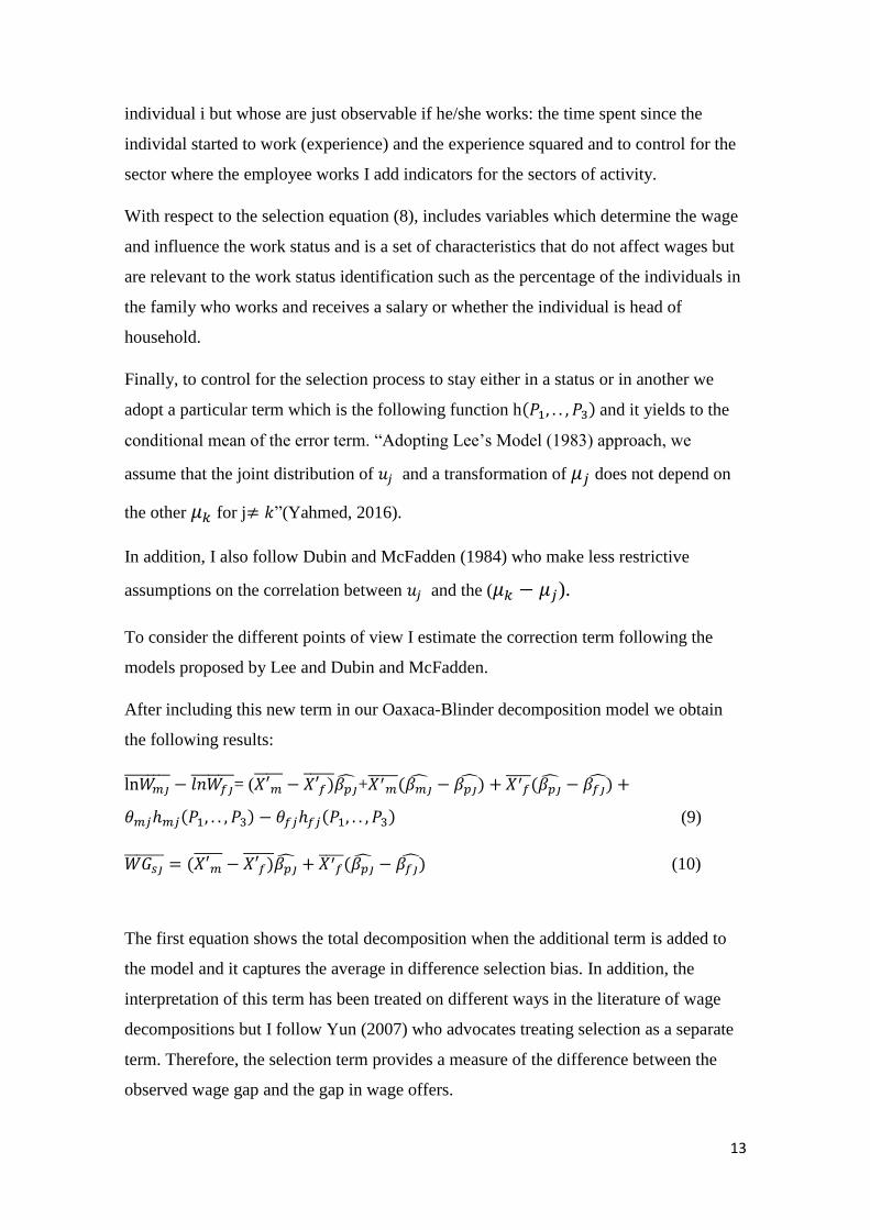
Finally, to control for the selection process to stay either in a status or in another we

adopt a particular term which is the following function h(𝑃1, . . , 𝑃3)and it yields to the

conditional mean of the error term. “Adopting Lee’s Model (1983) approach, we

assume that the joint distribution of 𝑢𝑗 and a transformation of 𝜇𝑗 does not depend on

the other 𝜇𝑘for j≠ 𝑘”(Yahmed, 2016).

In addition, I also follow Dubin and McFadden (1984) who make less restrictive

assumptions on the correlation between 𝑢𝑗 and the (𝜇𝑘 − 𝜇𝑗).

To consider the different points of view I estimate the correction term following the

models proposed by Lee and Dubin and McFadden.

After including this new term in our Oaxaca-Blinder decomposition model we obtain

the following results:

ln𝑊𝑚𝑗 − 𝑙𝑛𝑊𝑓𝑗

= (𝑋′𝑚 − 𝑋′𝑓) 𝛽𝑝��+𝑋′𝑚

(𝛽𝑚�� − 𝛽𝑝𝑗) + 𝑋′𝑓

(𝛽𝑝�� − 𝛽𝑓𝑗) +

𝜃𝑚𝑗ℎ𝑚𝑗(𝑃1, . . , 𝑃3) − 𝜃𝑓𝑗ℎ𝑓𝑗(𝑃1, . . , 𝑃3) (9)

𝑊𝐺𝑠𝑗 = (𝑋′𝑚 − 𝑋′𝑓) 𝛽𝑝�� + 𝑋′𝑓

(𝛽𝑝�� − 𝛽𝑓𝑗) (10)

The first equation shows the total decomposition when the additional term is added to

the model and it captures the average in difference selection bias. In addition, the

interpretation of this term has been treated on different ways in the literature of wage

decompositions but I follow Yun (2007) who advocates treating selection as a separate

term. Therefore, the selection term provides a measure of the difference between the

observed wage gap and the gap in wage offers.

14

On the other hand, the second one presents the wage gap between male and female

individuals and it is not equal to that showed in equation (3). The main difference with

that one is that (10) estimate consistently the coefficients following the treatment for

selection.

3.3 Identification

In this section I explain some exclusion restrictions needed to identify the effect of

selection and vanish the selection bias from the wage estimates without relying on the

functional forms. These restrictions mean that there are some variables which affect

wages only through the status where they stay. Since I am performing a replication from

Yahmed (2016) I try to use the same variables as long as they are available.

Therefore, the excluded variables I chose are the following. The first one is whether the

individual is head of household, because it may influence to stay either in a status or in

another due to the fact his/her income is the main one.

The second variable I use is the number of people compose the household, because I

think that, if this value is higher, the individual will consider working in the formal

sector to give to his/her family more security. In this sense, I also use the share of

individuals who receives income from working.

Finally, I consider two more variables where the first one represents the individual’s

civil status, because there is evidence that women may be conditionated to choose the

sector to work depending on whether they are married. The last variable I include is the

region where the individual was born because it may represent a strong characteristic to

be either a formal worker or an informal one.

15

4. Descriptive statistics

In this section I show some different specifications of the individuals to defend the

model I estimate in the final part of the paper. I present these specifications through the

following tables and distribution graphs.

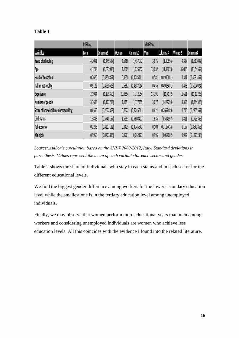
Table 1 shows some main variables from own characteristics to job related ones. In first

place, we may observe that in both sectors the mean of years of schooling are higher for

women than for men, this may be explained by the fact of those women who want to

work are high-skill workers. Moreover, these means are lower for the informal labour

market such as Addabbo and Favaro in 2011 suggested.

Regarding the mean of age in each sector we may observe that it is much higher for the

formal sector than for the informal one where this value is around thirty four years. A

plausible explanation of this may be that as people get older give preference the stability

received from the social security. The variable which represents whether the individual

is the head of household takes higher values for men than for women in both sectors.

This may agree with cultural believes about it has to be the man who brings income to

home meanwhile the woman cares about the children and the house.

If we focus on Italian individuals we may observe that there are more ones in the formal

labor market than in the informal ones. A job related characteristic we may looking at is

experience average for each sector and, we may observe that the value shows a higher

value (around 21 years) for the formal sector than for the informal one (around 12

years).

According to the composition of household we may observe to the number of people are

composed and the share of household member who are working and the values they

take are really similar for both sectors.

Finally, I focus on the public sector because it does not have to have informal labour

market but the question I am using may lead to mistake because it does not include

companies in which the government is a stakeholder, such as the postal service and the

national railways. Regarding the data we may observe that it is higher the share of

women working in this sector than the share of men. I also present whether the

individual works in his/her main job and we may observe that almost all the individuals

interviewed do.

16

Table 1

FORMAL INFORMAL

Variables Men Columna2 Women Columna1 Men Columna3 Women5 Columna4

Years of schooling 4,2041 (1,445537) 4,6466 (1,457972) 3,675 (1,39856) 4,327 (1,517042)

Age 4,1788 (1,097993) 4,1569 (1,025952) 33,632 (11,33673) 35,006 (11,54569)

Head of household 0,7626 (0,4254857) 0,3550 (0,4785411) 0,581 (0,4936601) 0,311 (0,4631467)

Italian nationality 0,5122 (0,4998626) 0,5362 (0,4987014) 0,456 (0,4983481) 0,498 (0,5004024)

Experience 2,1944 (1,179359) 20,0354 (11,12954) 13,791 (11,7172) 11,611 (11,12225)

Number of people 3,3686 (1,177708) 3,1451 (1,177455) 3,677 (1,422259) 3,364 (1,344346)

Share of household members working 0,6550 (0,2672368) 0,7522 (0,2245641) 0,621 (0,2657489) 0,746 (0,2305557)

Civil status 1,3833 (0,5748167) 1,5283 (0,7608407) 1,635 (0,534897) 1,811 (0,723365)

Public sector 0,2298 (0,4207182) 0,3425 (0,4745842) 0,109 (0,3117414) 0,157 (0,3643865)

Main job 0,9950 (0,0707806) 0,9961 (0,062127) 0,995 (0,067002) 0,982 (0,1323286)

Source:.Author’s calculation based on the SHIW 2000-2012, Italy. Standard deviations in

parenthesis. Values represent the mean of each variable for each sector and gender.

Table 2 shows the share of individuals who stay in each status and in each sector for the

different educational levels.

We find the biggest gender difference among workers for the lower secondary education

level while the smallest one is in the tertiary education level among unemployed

individuals.

Finally, we may observe that women perform more educational years than men among

workers and considering unemployed individuals are women who achieve less

education levels. All this coincides with the evidence I found into the related literature.

17

Table 2

All Unemployed Formal Informal

Men Women Men Women Men Women Men Women

Primary education 11.58 16.93 17.23 24.39 7.40 4.99 14.64 8.09

Lower secondary education 38.06 32.97 42.07 38.46 35.68 23.84 46.40 31.72

Upper and post secondary education 40.06 38.62 34.02 30.92 44.72 51.86 32.09 45.15

Tertiary education 10.31 11.48 6.68 6.23 12.20 19.32 6.87 15.05

Source: Author’s calculation based on the SHIW 2000-2012, Italy. It shows the share of

individuals who stay in each status and in each sector for the different educational levels.

Table 32 presents the regional unemployment rate by gender and different educational

levels. We may observe that this rate is much higher for female individuals in all

education groups. Despite of this, the value gets lower for the higher educational levels.

Therefore, the biggest difference occurs in primary education level. In order to identify

the impact of lower labour demand I include an index which represents the regional

unemployment rate for educational levels as control variables.

To complete the data description I present some distributions to observe how the wages

are distributed across the sample.

We may observe that, among formal workers, the wage distribution is really similar

although is a little bit fatter on the left side for women. If we look at the informal sector

we may appreciate that women wage distribution is shifted farther to the left showing us

that there exists a distributional gender wage gap.

Moreover, this fact occurs at all educational levels in both sectors since we may

observe. In the next sections I show whether this gap is different between the sectors

and whether it occurs even when controlling for some different variables.

2 Table 3 is showed in the Appendix

18

Figure 1

Source: Author’s calculation based on the SHIW 2000-2012, Italy. It shows wage distribution

for each sector and gender. The left-side figure represents the formal sector and the right-side

one, the informal sector.

Figure 2

0.2

.4.6

.81

Den

sity

0 2 4 6ln_w_hour

male

female

kernel = epanechnikov, bandwidth = 0.0487

Kernel density estimate

0.2

.4.6

.8

Den

sity

0 1 2 3 4 5ln_w_hour

male

female


Kernel density estimate0

.51

1.5

Den

sity

0 1 2 3 4ln_w_hour

male

female



0.5

11

.5

Den

sity

0 1 2 3 4 5ln_w_hour

male

female



19


for each gender among formal workers by different educational level. The images are organized

as Primary education, Lower secondary education, Upper and post secondary education and

Tertiary education, respectively.

Figure 3


for each gender among informal workers by different educational level. The images are

0.5

11

.5

Den

sity

0 2 4 6ln_w_hour

male

female



0.5

11

.5

Den

sity

0 2 4 6ln_w_hour

Male

Female



0.2

.4.6

.81

Den

sity

0 1 2 3 4ln_w_hour

male

female



0.2

.4.6

.81

Den

sity

0 1 2 3 4 5ln_w_hour

male

female



0.2

.4.6

.8

Den

sity

0 1 2 3 4 5ln_w_hour

male

female



0.5

11

.5

Den

sity

0 2 4 6ln_w_hour

male

female



20

organized as Primary education, Lower secondary education, Upper and post secondary

education and Tertiary education, respectively.

21

5. Results

In this section I show the estimations of the model presented in the “Estimation

Strategy” section.

I start the empirical analysis by commenting the multinomial logit estimates for each

sector and gender.

In first place, if we look at the formal labour market coefficients for men we may

appreciate that the probability of being in this status is different for the individuals

depending on their characteristics. This is clear because all the coefficients are

significant at all levels.

Moreover, all the signs make sense. For instance, we expect that if the individual is the

head of household, the probability to work in the formal sector increases because it

guarantees some stability.

In second place, if we focus on the informal labour market, we may observe that we

obtain almost the same results as in the formal sector. In this sense, it is worth

mentioning the fact of the educational level obtained has opposite effects in both

sectors, showing a negative effect when this level increases.

Regarding women’s results, we may observe that in the formal labour market the

variables included in the equation are significant and the signs are the expected.

Comparing them with the informal estimates we may observe that the results are the

same, even the educational level sign.

Since I mention above, the first equation I estimate the raw gender wage gap with no

control variables for the formal and informal sector. In this equations, the coefficient

obtained represents the gap.

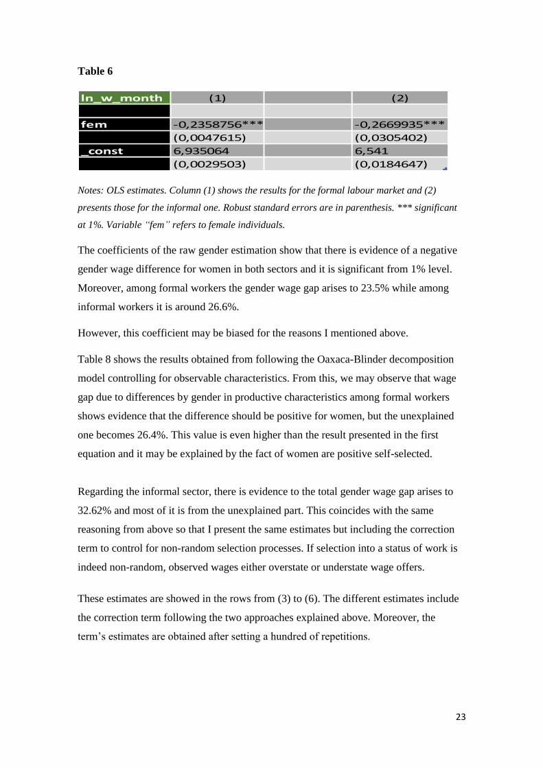
If we look at Table 6 the coefficients of the raw gender wage gap estimation show that

there is evidence of a negative gender wage difference for women in both sectors and it

is significant from 1% level. Moreover, among formal workers the gender wage gap

arises to 23.5% while among informal workers it is around 26.6%.

22

Table 4

Formal status Coef. Std. Err. z P>z [95% Conf. Interval]

Age 0,60117 0,0079375 75,74 0 0,5856163 0,6167308

Ages square -0,00798 0,0000956 -83,43 0 -0,0081642 -0,0077894

Level of education 0,16798 0,0103494 16,23 0 0,1476933 0,1882623

Italian 0,15770 0,0296269 5,32 0 0,0996321 0,2157675

Head of household 2,51256 0,0418568 60,03 0 2,430517 2,5945920

Number of components 0,39458 0,0159806 24,69 0 0,3632588 0,4259014

Share of household members working2,98332 0,0712471 41,87 0 2.843.675 3.122.959

Civil status -0,63015 0,0332102 -18,97 0 -0,6952397 -0,5650581

Birth municipality -0,13705 0,0175906 -7,79 0 -0,1715248 -0,1025711

_cons -1,32722 0,2101364 -63,16 0 -1.368.409 -1.286.037

Notes: Multinomial logit estimates for the formal sector based on the SHIW for 2000-2012,

Italy. All the coefficients are statiscally significant at 0%, 5% and 10%.

Table 5

Informal status Coef. Std. Err. z P>z [95% Conf. Interval]

Age 0,40892 0,0211 19,41 0 0,3676263 0,4502194

Ages square -0,00631 0,0003 -23,11 0 -0,0068475 -0,0057767

Level of education -0,10228 0,0302 -3,39 0,001 -0,1614114 -0,0431536

Italian 0,04404 0,0761 0,58 0,563 -0,1050993 0,1931708

Head of household 2,48686 0,1021 24,35 0 2,286683 2,687037

Number of components 0,48028 0,0363 13,24 0 0,4091786 0,5513811

Share of household members working 3,25094 0,1782 18,24 0 2.901.665 360.022

Civil status -0,36761 0,0945 -3,89 0 -0,5527653 -0,1824499

Birth municipality 0,83811 0,0579 14,46 0 0,7245482 0,9516813

_cons -1,38666 0,5202 -26,66 0 -1,488616 -1,284694

Notes: Multinomial logit estimates for the formal sector based on the SHIW for 2000-2012,

Italy. All the coefficients are statiscally significant at 1%, 5% and 10% except the Italian

nationality. This is significant just at 10% level.

23

Table 6

ln_w_month (1) (2)

fem -0,2358756*** -0,2669935***

(0,0047615) (0,0305402)

_const 6,935064 6,541

(0,0029503) (0,0184647)

Notes: OLS estimates. Column (1) shows the results for the formal labour market and (2)

presents those for the informal one. Robust standard errors are in parenthesis. *** significant

at 1%. Variable “fem” refers to female individuals.

The coefficients of the raw gender estimation show that there is evidence of a negative

gender wage difference for women in both sectors and it is significant from 1% level.

Moreover, among formal workers the gender wage gap arises to 23.5% while among

informal workers it is around 26.6%.

However, this coefficient may be biased for the reasons I mentioned above.

Table 8 shows the results obtained from following the Oaxaca-Blinder decomposition

model controlling for observable characteristics. From this, we may observe that wage

gap due to differences by gender in productive characteristics among formal workers

shows evidence that the difference should be positive for women, but the unexplained

one becomes 26.4%. This value is even higher than the result presented in the first

equation and it may be explained by the fact of women are positive self-selected.

Regarding the informal sector, there is evidence to the total gender wage gap arises to

32.62% and most of it is from the unexplained part. This coincides with the same

reasoning from above so that I present the same estimates but including the correction

term to control for non-random selection processes. If selection into a status of work is

indeed non-random, observed wages either overstate or understate wage offers.

These estimates are showed in the rows from (3) to (6). The different estimates include

the correction term following the two approaches explained above. Moreover, the

term’s estimates are obtained after setting a hundred of repetitions.

24

Table 7

Coef. Robust SE z P>z [95% Conf. Interval]

difference 0,2410407*** 0,0086466 27,88 0 0,2240937 0,2579877

(1) explained -0,0235972*** 0,0061078 -3,86 0 -0,0355683 -0,0116261

unexplained 0,2646379*** 0,0079006 33,5 0 0,249153 0,2801228

difference 0,3262214*** 0,0574351 5,68 0 0,2136507 0,4387921

(2) explained 0,0721032 0,0511183 1,41 0,158 -0,0280869 0,1722932

unexplained 0,2541182*** 0,0677344 3,75 0 0,1213612 0,3868753

difference 0,2257217*** 0,0089585 25,2 0 0,2081633 0,2432801

(3) explained -0,0062772 0,0066391 -0,95 0,344 -0,0192895 0,0067351

unexplained 0,2319989*** 0,0082761 28,03 0 0,215778 0,2482198

difference 0,335007*** 0,0638962 5,24 0 0,2097727 0,4602414

(4) explained 0,1161096* 0,060777 1,91 0,056 -0,0030111 0,2352303

unexplained 0,2188974*** 0,0759535 2,88 0,004 0,0700312 0,3677636

difference 0,2257217*** 0,0089585 25,2 0 0,2081633 0,2432801

(5) explained -0,0169073** 0,0065442 -2,58 0,01 -0,0297336 -0,004081

unexplained 0,242629*** 0,0082957 29,25 0 0,2263697 0,2588883

difference 0,335007*** 0,0638959 5,24 0 0,2097733 0,4602408

(6) explained 0,1200233** 0,0610742 1,97 0,049 0,00032 0,2397266

unexplained 0,2149837*** 0,076454 2,81 0,005 0,0651366 0,3648308

Notes: Oaxaca-Blinder decomposition estimates. Panel (1) and (2) show the results controlling

for observable characteristics for both sectors. Panel (3) and (4) present the estimation

controlling for non-random selection following Lee’s approach. Panel (5) and (6) the same than

(3) and (4) but following Dubin and McFadden’s model. Robust standard errors are in

parenthesis. *** significant at 1%. ** significant at 5%. * significant at 10%. These estimates

are based on SHIW data for 2000-2012. Control variables used are educational level, age, age

square, potential experience, potential experience square, Italian nationality and regional

unemployment rate. Selection equation: controlling for the same previous variables and head of

household, number of components in the household, share of household members working, civil

status and birth municipality.

25

As expected, among formal workers there is evidence of a decrease in the gap which

supports the idea that women are positively selected. This leads to larger results,

therefore, there is evidence that gender wage gap is overestimated. This may be

explained by the fact of employers offer lower wages to women because they have a

higher quit probability so that they expect to face higher labour costs.

However, among informal workers I can appreciate that there is evidence that total gap

is also larger than when controlling for observable characteristics. Moreover, the

unexplained part shows a decrease in both cases. This reduction comes from the

inclusion of the correction term which captures the non-random selection processes.

In addition, this is related with the idea mentioned above that women are positively

selected which means that only those who are more prepared work. Therefore, these

results are consistently estimated and support the evidence of wage discrimination

against women.

26

6. Robustness checks

To complete the investigation and checking whether the results obtained are reliable I

perform some estimations by considering another definition of informal workers. I use a

ratio between the same variable I use in the model and the potential experience and take

into account the percentiles of it. I apply this quantile decomposition to analyse the

changes of the gender wage gap at different points of the wage distribution.

I estimate the gender wage gap by using the Oaxaca and Blinder decomposition model

controlling for observable characteristics as I do in the first part of the previous section.

The table shows the results obtained and they present evidence that the gap is higher as

workers perform a higher percentage of their worklife in the informal sector. Moreover,

we may observe that this discrimination decreases when we look more to the right of the

distribution. In other words, when workers have been fewer years in this sector, the gap

is smaller.

Finally, we may observe that the unexplained part represents most of this difference. In

addition, this wage gap due to differences in returns for the same characteristics presents

smaller values when the observed part of the distribution is closer to the bottom.

27

Table 8

Coef. Robust SE z P>z [95% Conf. Interval]

difference .3308049 .0863322 3.83 0.000 .1615969 .5000129

p05 explained -.106175 .059006 -1.80 0.072 -.2218246 .0094745

unexplained .43698 .0792307 5.52 0.000 .2816907 .5922693

difference .3197186 .0368393 8.68 0.000 .2475149 .3919223

p15 explained -.0611753 .0229195 -2.67 0.008 -.1060968 -.0162539

unexplained .3808939 .0355006 10.73 0.000 .311314 .4504739

difference .2959545 .0245648 12.05 0.000 .2478084 .3441006

p25 explained -.0522043 .015873 -3.29 0.001 -.0833148 -.0210938

unexplained .3481588 .0240867 14.45 0.000 .3009497 .3953679

difference .292619 .0195673 14.95 0.000 .2542677 .3309703

p35 explained -.0494643 .0130548 -3.79 0.000 -.0750514 -.0238773

unexplained .3420833 .0186921 18.30 0.000 .3054476 .3787191

difference .2679861 .0164273 16.31 0.000 .2357891 .3001831

p45 explained -.0508064 .0114458 -4.44 0.000 -.0732397 -.0283731

unexplained .3187925 .0158132 20.16 0.000 .2877992 .3497858

Notes: Oaxaca-Blinder decomposition estimates.. Robust standard errors are in parenthesis.

*** significant at 1%. ** significant at 5%. * significant at 10%. These estimates are based on

SHIW data for 2000-2012. Control variables used are educational level, age, age square,

potential experience, potential experience square, Italian nationality and regional

unemployment rate. Selection equation: controlling for the same previous variables and head of

household, number of components in the household, share of household members working, civil

status and birth municipality.

28

7. Conclusions

After presenting all the results I can conclude that there is evidence of wage

discrimination in the formal and informal labour market during the period from 2000-

2012 in Italy.

Despite of the existence of it, I obtain that this gap is smaller when I control for non-

random selection processes following different models proposed by Lee, Dubin and

McFadden. As I mention above, it supports the idea of positive selection and presents

evidence of overestimating gender wage gap when just controlling for observable

characteristics.

In addition, this gap is almost completely unexplained by observed characteristics,

applying SHIW data for the mentioned period. I also provide evidence across the

distribution and it showed the discrimination is larger among workers who spent most

of their worklife in the undeclared sector.

If I compare the results obtained in this paper with Yahmed’s ones I may observe that

they are different. Yahmed (2016) present a qualitatively different gender wage gap

from Brazil than the one I show here in formal and informal sectors (5% and 13% vs

22.5% and 33.5%). These differences may be explained by the different laws are in each

country and how they influence wage offers by gender. Another interesting explanation

may come from the different development levels the countries have.

Moreover, if I revise gender wage gap literature I find that some investigations suggest

a smaller gap (Piazzalunga and Di Tommaso, 2015; Mussida and Picchio, 2014).

However, when they control for non-random selection, I think that the different results

are due to the fact of they just consider two statuses and perform the model proposed by

Heckman (1974).

In this sense, it would be interesting perform some estimations by using subpopulations

to check whether the size of the discrimination. These subpopulations could be either

immigrant individuals or classifying by civil status because some studies have found

that female individuals have different incentives to invest in human capital. Another

interesting idea would be considering a country where there exists the same laws for

men and women when they have children. By using this, I think it is able to find

whether this policy gets to reduce wage discrimination.

29

Finally, I perform the investigation by considering the monthly wages but I checked that

there is evidence that considering hourly ones the results are qualitatively similar.

30

8. References

OOSTENDORP, R., 2009. GLOBALIZATION AND THE GENDER WAGE GAP. THE WORLD

BANK ECONOMIC REVIEW 23, 141–161. DOI:10.1093/WBER/LHN022

EDO, A., TOUBAL, F., 2017. ’IMMIGRATION AND THE GENDER WAGE GAP. EUROPEAN

ECONOMIC REVIEW 92, 196–214. DOI:10.1016/J.EUROECOREV.2016.12.005

NYHUS, E.K., PONS, E., 2012. PERSONALITY AND THE GENDER WAGE GAP. APPLIED

ECONOMICS 44, 105–118. DOI:10.1080/00036846.2010.500272

MUSSIDA, C., PICCHIO, M., 2014. THE TREND OVER TIME OF THE GENDER WAGE GAP IN

ITALY. EMPIRICAL ECONOMICS 46, 1081–1110. DOI:10.1007/S00181-013-0710-9

DEL BONO, E., VURI, D., 2011. JOB MOBILITY AND THE GENDER WAGE GAP IN ITALY.

LABOUR ECONOMICS 18, 130–142. DOI:10.1016/J.LABECO.2010.06.002

VON STACKELBERG, H., 2011. MARKET STRUCTURE AND EQUILIBRIUM, MARKET

STRUCTURE AND EQUILIBRIUM. SPRINGER BERLIN HEIDELBERG. DOI:10.1007/978-3-642-

12586-7

COTTER, DAVID A., JOANN DEFIORE, JOAN M. HERMSEN, BRENDA MARSTELLER

KOWALEWSKI, AND REEVE VANNEMAN. "ALL WOMEN BENEFIT: THE MACRO-LEVEL

EFFECT OF OCCUPATIONAL INTEGRATION ON GENDER EARNINGS EQUALITY." AMERICAN

SOCIOLOGICAL REVIEW 62, NO. 5 (1997): 714-34.

HIRSCH, B. GENDER WAGE DISCRIMINATION. IZA WORLD OF LABOR 2016: 310 DOI:

10.15185/IZAWOL.310

LIVANOS, I., NÚÑEZ, I., 2012. THE EFFECT OF HIGHER EDUCATION ON THE GENDER

WAGE GAP. INTERNATIONAL JOUNRAL OF EDUCATION ECONOMICS AND DEVELOPMENT

3. DOI:10.1353/JDA.2015.0072

ENSTE, D. THE SHADOW ECONOMY IN INDUSTRIAL COUNTRIES. IZA WORLD OF LABOR

2015: 127 DOI: 10.15185/IZAWOL.127

PETERSEN, T., MORGAN, L.A., 1995. SEPARATE AND UNEQUAL: OCCUPATION-

ESTABLISHMENT SEX SEGREGATION AND THE GENDER WAGE GAP SEPARATE AND

UNEQUAL: OCCUPATION-ESTABLISHMENT SEX SEGREGATION AND THE GENDER WAGE

GAP’. SOURCE: AMERICAN JOURNAL OF SOCIOLOGY 101, 329–365.

31

HORRACE, W.C., OAXACA, R.L., 2001. INTER-INDUSTRY WAGE

DIFFERENTIALS AND THE GENDER WAGE GAP: AN IDENTIFICATION

PROBLEM. INDUSTRIAL & LABOR RELATIONS REVIEW 54, 611–618.

ARSHAD, M.N.M., GHANI, G.M., 2015. RETURNS TO EDUCATION AND WAGE

DIFFERENTIAL IN MALAYSIA. THE JOURNAL OF DEVELOPING AREAS 49, 213–223.

DOI:10.1080/0003684042000217571

BOURGUIGNON, F., FOURNIER, M., GURGAND, M., 2007. SELECTION BIAS CORRECTIONS BASED

ON THE MULTINOMIAL LOGIT MODEL: MONTE CARLO COMPARISONS. JOURNAL OF ECONOMIC

SURVEYS 21, 174–205. DOI:10.1111/J.1467-6419.2007.00503.X

32

9. Appendix

Table 3

Unemploy

ment rat

ePrimary

education

Lower sec

ondary ed

ucationU

pper and p

ost second

ary educa

tionTertia

ry educatio

nTotal

Male

0,3858522

0,3775373

0,3684616

0,367608

0,3738414

Female

0,6277226

0,6013935

0,5791982

0,5715309

0,5938517

Sourc

e: A

uth

or’

s ca

lcula

tion b

ase

d o

n t

he

SH

IW 2

00

0-2

01

2,

Italy

. T

he

regio

nal

unem

plo

ymen

t ra

te b

y gen

der

and e

duca

tional

leve

l

UNIVERSIDAD DE ALICANTE FACULTAD DE CIENCIAS ECONÓMICAS … · UNIVERSIDAD DE ALICANTE FACULTAD DE...

Documents

Transcript of UNIVERSIDAD DE ALICANTE FACULTAD DE CIENCIAS ECONÓMICAS … · UNIVERSIDAD DE ALICANTE FACULTAD DE...