Unit6-KCV
44
6. 1 Intro duct ion A.C Circuits made up of resistors, inductors and capacitors are said to be resonant circuits when the current drawn from the supply is in phase with the impressed sinusoidal voltage. Then 1. the resultan t reactanc e or susceptance is zero. 2. the circuit beh ave s as a resistive cir cuit. 3. the powe r factor is uni ty . A second order series resonant circuit consists of , and in series. At resonance, voltages across and are equal and opposite and these voltages are many times greater than the applied voltage. They may present a dangerous shock hazard. A second order parallel resonant circuit consists of and in par all el. At res ona nce , currents in and are circulating currents and they are considerably lar ger than the input current. Unless proper consideration is given to the magnitude of these currents, they may become very large enough to destroy the circuit elements. Resona nce is the phenomeno n which finds its applic ations in communicati on circuits: The ability of a radio or Television receiver (1) to select a particular frequency or a narrow band of frequencies transmitted by broad casting stations or (2) to suppress a band of frequencies from other broad casting stations, is based on resona nce. Thus resonance is desired in tuned circuits, design of filters, signal processing and control engi nee ring. But it is to be avoi ded in other circuits. It is to be noted tha t if = 0 in a series circuit, the circuits acts as a short circuit at resonance and if = in parallel circuit, the circuit acts as an open circuit at resonanc e.
Transcript of Unit6-KCV

8/12/2019 Unit6-KCV
http://slidepdf.com/reader/full/unit6-kcv 1/44
6.1 Introduction
A.C Circuits made up of resistors, inductors and capacitors are said to be resonant circuits when
the current drawn from the supply is in phase with the impressed sinusoidal voltage. Then
1. the resultant reactance or susceptance is zero.
2. the circuit behaves as a resistive circuit.
3. the power factor is unity.
A second order series resonant circuit consists of ,
and
in series. At resonance, voltages
across and
are equal and opposite and these voltages are many times greater than the applied
voltage. They may present a dangerous shock hazard.
A second order parallel resonant circuit consists of
and in parallel. At resonance,
currents in and are circulating currents and they are considerably larger than the input current.
Unless proper consideration is given to the magnitude of these currents, they may become very
large enough to destroy the circuit elements.
Resonance is the phenomenon which finds its applications in communication circuits: The
ability of a radio or Television receiver (1) to select a particular frequency or a narrow band of
frequencies transmitted by broad casting stations or (2) to suppress a band of frequencies from
other broad casting stations, is based on resonance.
Thus resonance is desired in tuned circuits, design of filters, signal processing and control
engineering. But it is to be avoided in other circuits. It is to be noted that if = 0 in a series
circuit, the circuits acts as a short circuit at resonance and if = in parallel circuit,
the circuit acts as an open circuit at resonance.

8/12/2019 Unit6-KCV
http://slidepdf.com/reader/full/unit6-kcv 2/44
452 | Network Analysis
6.2 Transfer Functions
As ω is varied to achieve resonance, electrical quantities are expressed as functions of ω, normally
denoted by F ( jω) and are called transfer functions. Accordingly the following notations are used.
Z ( jω) = V ( jω)
I ( jω) = Impedance function
Y ( jω) = I ( jω)
V ( jω) = Admittance function
G( jω) = V 2( jω)
V 1( jω) = Voltage ratio transfer function
α( jω) = I 2( jω)I 1( jω)
= Current ratio transfer function
If we put jω = s then the above quantities will be Z (s), Y (s), G(s), α(s) respectively. These
are treated later in this book.
6.3 Series Resonance
Fig. 6.1 represents a series resonant circuit.
Resonance can be achieved by
1. varying frequency ω
2. varying the inductance L
3. varying the capacitance C Figure 6.1 Series Resonant Circuit
The current in the circuit is
I = E
R + j(X L −X C ) =
E
R + jX
At resonance, X is zero. If ω0 is the frequency at which resonance occurs, then
ω0L = 1
ω0C or ω0 =
1√ LC
= resonant frequency.
The current at resonance is I m = V
R = maximum current.
The phasor diagram for this condition is shown in Fig. 6.2.
The variation of current with frequency is shown in Fig. 6.3.
Figure 6.2 Figure 6.3

8/12/2019 Unit6-KCV
http://slidepdf.com/reader/full/unit6-kcv 3/44
Resonance | 453
It is observed that there are two frequencies, one above and the other below the resonant
frequency, ω0 at which current is same.
Fig. 6.4 represents the variations of X L = ωL;X C = 1
ωC and |Z | with ω.
From the equation ω0 = 1√ LC
we see that any constant product of L and C give a particular
resonant frequency even if the ratio L
C is different. The frequency of a constant frequency source
can also be a resonant frequency for a number of L and C combinations. Fig. 6.5 shows how the
sharpness of tuning is affected by different L
C ratios, but the product LC remaining constant.
Figure 6.4 Figure 6.5
For larger L
C ratio, current varies more abruptly in the region of ω0. Many applications call for
narrow band that pass the signal at one frequency and tend to reject signals at other frequencies.
6.4 Bandwidth, Quality Factor and Half Power Frequencies
At resonance I = I m and the power dissipated is
P m = I 2
mR watts.
When the current is I = I m√
2power dissipated is
P m
2 =
I 2mR
2 watts.
From ω − I characteristic shown in Fig. 6.3, it is observed that there are two frequencies
ω1 and ω2 at which the current is I = I m√
2. As at these frequencies the power is only one half of
that at ω0, these are called half power frequencies or cut off frequencies.
The ratio, current at half power frequencies
Maximum current =
I m√ 2I m
= 1√ 2
When expressed in dB it is 20 log 1√ 2= −3dB.

8/12/2019 Unit6-KCV
http://slidepdf.com/reader/full/unit6-kcv 4/44
454
Network Analysis
Therefore 1 and
2 are also called 3 dB frequencies.
As
2=
2
, the magnitude of the impedance at half-power frequencies is
2 = + (
)
Therefore, the resultant reactance, =
= .
The frequency range between half - power frequencies is 2 1, and it is referred to as
passband or band width.
BW = 2 1 =
The sharpness of tuning depends on the ratio
, a small ratio indicating a high degree of
selectivity. The quality factor of a circuit can be expressed in terms of and of the inductor.
Quality factor = = 0
Writing 0 = 2 0 and multiplying numerator and denominator by
1
2
2
, we get,
= 2 0
12
2
12
2
= 2
12
2
12
2
= 2
Maximum energy stored
total energy lost in a period
Selectivity is the reciprocal of
.As =
0
and 0 = 1
0
= 1
0
and since 0 = 1
, we have
= 1
6.5 Expressions for ω1 and ω2, and Bandwidth
At half power frequencies 1 and 2,
=
2
=
2 + (
)2
1
2
∴
= i e
1
=
At = 2, = 2
1
2
Simplifying,
22 2 1 = 0

8/12/2019 Unit6-KCV
http://slidepdf.com/reader/full/unit6-kcv 5/44
Resonance
455
Solving, we get
2 = +
2
2 + 4
2
=
2
+
2
2
+ 1
(6.1)
Note that only + sign is taken before the square root. This is done to ensure that 2 is always
positive.
At = 1,
= 1
1
1
21 + 1 1 = 0
Solving 1 = +
2
2 + 4
2
=
2
+
2
2
+ 1
(6.2)
While determining 1, only positive value is considered.
Subtracting equation(6.1) from equation (6.2), we get
2 1 =
= Band width.
Since = 0
, Band width is expressed as
= 2 1 =
= 0
and therefore = 0
2 1
= 0
Multiplying equations (6.1) and (6.2), we get
1 2 =
2
4
2 +
1
2
4
2 =
1
=
20
or 0 =
1 2
The resonance frequency is the geometric mean of half power frequencies.
Normally
2
1
in which case
5
Then 1
2
+
1
and 2
2
+ 1
=
2
+ 0 and 2 =
2
+ 0
∴ 0 = 1 + 2
2 = Arithmetic mean of 1 and 2
Since
= 0
, Equations for 1 and
2 as given by equations (6.1) and (6.2) can be expressed
in terms of as
2 = 0
2
+
0
2
2
+
20

8/12/2019 Unit6-KCV
http://slidepdf.com/reader/full/unit6-kcv 6/44
456
Network Analysis
= 0
1
2
+
1 +
1
2
2
Similarly 1 = 0
1
2
+
1 +
1
2
2
Normally,
2
1
and then 5.
Consequently
1 and
2 can be approximated as
1
2
+
1
=
2
+ 0 =
2 + 0
2
2
+
1
= +
2
+ 0 =
2 + 0
so that 0 =
1 + 2
2
6.6 Frequency Response of Voltage across L and C
As frequency is varied, both the voltages across and increase with frequency upto 0 and
they are equal at 0 But their maximum values do not occur at 0
reaches its maximum at 0 and
reaches its maximum at 0. This can be verified by calculating the frequency
at which each occurs.
6.7 Expression for ω at which V
is Maximum
Current in the circuit shown in Figure 6.1 is
=
2 +
1
2
Voltage across is
= =
2 +
1
2
Squaring
2
=
2
2
2
2 +
1
2
This is maximum when
2
= 0

8/12/2019 Unit6-KCV
http://slidepdf.com/reader/full/unit6-kcv 7/44
Resonance
457
That is,
2
2
2 +
1
2
2
2
2
1
+ 1
2
= 0
2 +
1
2
=
1
+ 1
2 +
2
2 + 1
2
2 2
=
2
2
1
2
2
2
2
2 + 1 2
2 = 1
or
2(2
2
2) = 2
2 = 22
2
2
= 1
1
2
2
Let this frequency be
.
Then
2
=
20
1
1
12
2
= 0
1
1
12
2
That is,
0.
6.8 Expression for ω at which V
is Maximum
Now
=
2 +
2
1
2
2
=
2
2
2
2 +
1
2
This is maximum when
(
2
) = 0
That is,
2
2
2
2
1
1
2
+ 2
2 +
1
2
= 0
2 +
1
2
=
1
+ 1

8/12/2019 Unit6-KCV
http://slidepdf.com/reader/full/unit6-kcv 8/44
458
Network Analysis
2 +
2
2 + 1
2
2 2
= 1
2
2
2
2
2
2
2 +
2 = 2
2 = 2
2
2
2 =
1
2
2
2
= 1
1
2
2
=
20
1
1
2
2
Let this frequency be
= 0
1
1
2
2
i e
0
Variations of
and
as functions of
are shown in Fig. 6.6.Figure 6.6
We know that
=
2
2
2 + (
2
1)2
2
2
=
2
2
2 + (
2 1)2
(6.3)
Consider
2
2
2 + (
2
1)2 and at =
. Then equation(6.3) becomes
2
2
2 + (
2
1)2 =
20
1
1
2
2
2
2 +
20
1
1
2
2
1
2
= 1
2
1
1
2
2
+
20
1
1
2
2
1
20
1
2
= 1
2
1
1
2
2
+
1
4
4
= 1
2
1
2
4 +
1
4
4 =
1
2
1
1
4
2
since 1
=
20 and 0 =
1
Substituting the above expression in the denominator of equation (6.3), we get
=
1
14
2
6.9 Selectivity with Variable L
In a series resonant circuit connected to a constant voltage, with a constant frequency, when is
varied to achieve resonance, the following conditions prevail:

8/12/2019 Unit6-KCV
http://slidepdf.com/reader/full/unit6-kcv 9/44
Resonance
459
1.
is constant and =
2 +
2
when = 0.
2. With increase in
increases and
=
at
=
3. With further increase in proceeds to fall.
All these conditions are depicted in Fig. 6.7
max occurs at
0 but
max occurs at a point beyond 0.
at which
becomes a maximum is obtained in terms of
other constants.
=
2 + (
)2
1
2
2
=
2
2
2 + (
)2
Figure 6.7
This is maximum when
2
= 0.
Therefore
2 + (
)2
2
=
2
2(
)
2 +
2
+
2
2
=
2
Therefore
= 2 + 2
Let the corresponding value of is
.
Then
= (
2 +
2
)
and 0 = value of
at
0 such that
0 = 1
0
6.10 Selectivity with Variable C
In a series resonant circuit connected to a constant voltage, constant frequency supply, if
isvaried to achive resonance, the following conditions prevail:
1.
is constant.
2.
varies as inversely as
when = 0, = 0.
when =
1
, =
=
.
3. with further increase in
starts decreasing as shown in Fig. 6.8, where
is the value of
capacitance at maximum voltage across and
0 is the value of the capacitance at 0.

8/12/2019 Unit6-KCV
http://slidepdf.com/reader/full/unit6-kcv 10/44
460
Network Analysis
at which
becomes maximum can be determined in
terms of other circuit constants as follows.
=
2 + (
)2
2
=
2
2
2 + (
)2Figure 6.8
For maximim
2
= 0
Then
2 + (
)2
2
2
2(
)( 1) = 0
2 +
2
+
2
2
=
+
2
=
2 +
2
Let the correrponding value of be
.
Then
=
2 +
2
6.11 Transfer Functions
6.11.1 Voltage ratio transfer function of a series resonant circuit and frequency response
For the circuit shown in Fig. 6.9, we can
write
( ) = 0( )
( ) =
+
1
= 1
1 +
1
= 1
1 +
0
0
0 0
= 1
1 +
0
0
= 1
1 +
2
0
0
2
1
2
tan 1
0
0
Figure 6.9

8/12/2019 Unit6-KCV
http://slidepdf.com/reader/full/unit6-kcv 11/44
Resonance
461
Let be a measure of the deviation in
from
0. It is defined as
= 0
0=
0 1
Then
0
0
= ( + 1)
1
+ 1 =
( + 1)2 1
+ 1 =
2 + 2
+ 1
For small deviations from 0 1 Then,
0
0
2
Then ( ) = 11 + 2
= 1
1 + 4
2
2
tan 1 2
The amplitfude and phase response curves are as shown in Fig. 6.10.
Figure 6.10 (a) and (b): Amplitude and Phase response of a series resonance circuit
6.11.2 Impedance function
The Impedance as a function of
is given by
( ) = +
1
=
1 +
1
=
1 +
0
0
=
1 +
2
0
0
2
tan 1
0
0
For small deviations from 0, we can write
( ) [1 + 2 ] =
1 + 4
2
2
tan 1 2

8/12/2019 Unit6-KCV
http://slidepdf.com/reader/full/unit6-kcv 12/44
462
Network Analysis
6.12 Parallel Resonance
The dual of a series resonant circuit is often considered as a parallel resonant circuit and it is as
shown in Fig. 6.11.
The phasor diagram for resonance is shown in Fig. 6.12.
The admittance as seen by the current source is
( ) =
+
+
= 1
+
1
= +
Figure 6.11 Parallel Resonance Circuit Figure 6.12 Phasor Diagram
If the resonance occurs at 0
then the susceptance is zero. That is,
0
=
1
0
or
0 = 1
rad sec
At resonance,
0 =
0 = 0
and
=
0 +
0 = 0
The quality factor, as in the case of series resonant circuit is defined as
= 2
Maximum energy stored
Energy dissipated in a period
= 2
12
2
12
2m
= 2 0 = 0
Since 0 = 1
0
=
0
8/12/2019 Unit6-KCV
http://slidepdf.com/reader/full/unit6-kcv 13/44
Resonance
463
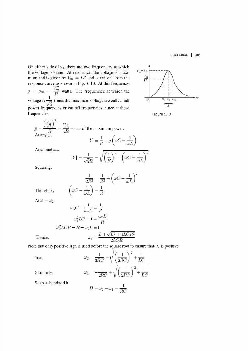
On either side of 0 there are two frequencies at which
the voltage is same. At resonance, the voltage is maxi-
mum and is given by
= and is evident from the
response curve as shown in Fig. 6.13. At this frequency,
=
=
2
watts. The frequencies at which the
voltage is 1
2times the maximum voltage are called half
power frequencies or cut off frequencies, since at these
frequencies, Figure 6.13
=
m
2
2
=
2
2
= half of the maximum power.
At any ,
= 1
+
1
At 1 and
2
= 1
2
=
1
2
+
1
2
Squaring,
1
2
2 =
1
2 +
1
2
Therefore
1
= 1
At = 2,
2
1
2
= 1
22 1 =
2
22 2 = 0
Hence 2 = +
2 + 4
2
2
Note that only positive sign is used before the square root to ensure that 2 is positive.
Thus 2 = 1
2
+
1
2
2
+ 1
Similarly 1 =
1
2
+
1
2
2
+ 1
So that, bandwidth
= 2 1 = 1

8/12/2019 Unit6-KCV
http://slidepdf.com/reader/full/unit6-kcv 14/44
464
Network Analysis
and 1 2 =
1
2
2
+ 1
1
2
2
= 1
=
20
Thus 0 =
1 2
As 0 = 1
and = 0 =
0
=
=
Since 1
2
=
2
2 =
2 +
2
2
+
20
and 1 =
2 +
2
2
+
20
Using = 0
,
2 = 0
1
2
+
1 +
1
2
2
and 1 = 0
1
2
+
1 +
1
2
2
6.13 Transfer Function and Frequency Response
The transfer function for a parallel RLC circuit shown in
Fig. 6.14. is ( ), the current ratio transfer function.
(
) =
0( )
1( ) =
1
( )
= 1
11
+
1
= 1
1 +
1
= 1
1 +
0
0
0
0 L
= 1
1 +
0
0
Figure 6.14 Parallel RLC Circuit
As in the case of series resonance, here also let
= 0
0=
0 1

8/12/2019 Unit6-KCV
http://slidepdf.com/reader/full/unit6-kcv 15/44
Resonance
465
then,
0
0
=
2 + 2
+ 1
For 1, for small deviations from 0
0
0
2
Therefore,
( ) = 1
1 +
2
6.14 Resonance in a Two Branch RL RC Parallel Circuit
Consider the two branch parallel circuit shown in Fig. 6.15. Let be the voltage across each of
the parallel circuit shown in the figure. The vector diagram at resonance is shown in Figure 6.1.
Figure 6.15 Two branch Parallel Circuit Figure 6.16
The admittance of the circuit is ( ) =
+
+
For resonance,
=
If this occurs at = 0,
then 0
2 +
20
2 =
1 0
2
+ 1
20
2
= 0
2
20
2 + 1
(1 +
20
2
2
) = (
2
+
20
2)
20(
2
2
2 ) =
2

8/12/2019 Unit6-KCV
http://slidepdf.com/reader/full/unit6-kcv 16/44
466 | Network Analysis
ω2
0 = R2
L C − 1
LC 2 R2
C − L2C
= 1
LC
R2
L C −L
(R2
C C −L
= 1
LC
R2
L − L
C
(R2
C − L
C
Therefore, ω0 = 1√
LC
R2
L − L
C
R2
C − L
C
This is the expression for resonant frequency. It is to be noted that
1. resonance is not possible for certain combination of circuit elements unlike in a series
circuit where resonance is always possible.2. resonance is also possible by varying of RL or RC .
Consider the case where
R2
C < L
C < R2
L
or
R2
L < L
C < R2
C
In both these cases, the quantity under radical is negative and therefore resonance is not pos-
sible.
The admittance at resonance of the above parallel circuit is
Y 0 =
RL
R2
L + X 2
L0
+ RC R2
C + X 2
C 0
S
where X L0 and X C 0 are the inductive and capacitive reactances respectively at resonance.
If RL = RC =
L
C
then ω0 = 1√
LC
as in R,L,C series circuit.
If RL = RC = L
C
which means
R2
L = R2
C = R2 = L
C = X LX C .
Then, BL − BC = X L
R2
L + X 2
L
− X C
R2
C + X 2
C
= 1
X L + X C − 1
X L + X C = 0

8/12/2019 Unit6-KCV
http://slidepdf.com/reader/full/unit6-kcv 17/44
Resonance
467
In this case, the circuit acts as a pure resistive circuit irrespective of frequency. That is, the
circuit is resonant for all frequencies.
In this case the circuit admittance is
=
2
+
2
+
2
+
2
=
2 +
2
+
2 +
2
4 +
2(
2
+
2
) +
2
2
=
2
2 +
2
+
2
2
4
+
2
(
2
+
2
)
=
2
2
2 +
2
+
2
2
2 +
2
+
2
= 1
=
or = =
6.14.1 Resonance by varying inductance
If resonance is achieved by varying only in the circuit shown in Figure 6.15 but with constant
current constant frequency source, then the condition for resonance is
=
2
+
2
=
2
+
2
=
2
where
2
=
2
+
2
Then
2
2
+
2
= 0
Solving, for
we get
=
2
4
4
2
2
2
Therefore =
2
2
4
4
2
2
since
=
The following conditions arise:
1. If
4
4
2
2
has two values for the circuit to resonate.
2. For
4
= 4
2
2
, = 1
2
2
for reasonance.
3. For
4
4
2
2
, No value of makes the circuit to resonate.

8/12/2019 Unit6-KCV
http://slidepdf.com/reader/full/unit6-kcv 18/44
468
Network Analysis
6.14.2 Resonance by varying capacitance
As in the previous case, we have at resonance„
=
2
+
2
=
2
where
2
=
2
+
2
Simplifying we get,
2
2
+
2
= 0
=
2
4
4
2
2
2
Therefore = 2
2
4
4
2
2
The following conditions arise:
1. For
4
4
2
2
, there are two values for to resonante.
2. For
44 = 4
2
2
, resonance occurs at =
2
2
.
3. For
4
4
2
2
, no value of makes the circuit to resonate.
6.14.3 Resonance by varying R
or R
It is often possible to adjust a two branch parallel combination to resonate by varying either
or
. This is because, when the supply is of constant current and, constant frequency, these
resistors control inphase and quadratare components of the currents in the two parallel paths.
From the condition
=
, we get
2
+
2
=
2
+
2
2
=
2
+
2
=
2 +
2
(6.4)
This equation gives the value of
for resonance when all other quantities are constant and
the term under radical is positive.
Similarly if only
is variable, keeping all other quantities constant, the value of
for
resonanace is given by
=
2
+
2
provided the term under radical is positive.

8/12/2019 Unit6-KCV
http://slidepdf.com/reader/full/unit6-kcv 19/44
Resonance | 469
6.15 Practical Parallel and Series Resonant Circuits
A practical resonant parallel circuit contains an inductive coil of resistance R and inductance L in
parallel with a capacitor C as shown in Fig. 6.17. It is called a tank circuit because it stores energy
in the magnetic field of the coil and in the electric field of the capacitor. Note that resistance RC
of the capacitor is negligibly small.
Condition for parallel resonance is shown by the phasor diagram of Fig. 6.18.
I C = I L sin φ
That is, BC = BL
⇒ ωL
R2 + ω2L2 = ωC.
Let the value of ω which satisfy this condition be ω0.
Then, R2 + ω2
0L2 =
L
C (6.5)
ω2
0 =
L
C − R2
1
L2 =
1
LC
1 − R2C
L
ω0 = 1
√ LC
1
−
R2C
L
(6.6)
Figure 6.17 Figure 6.18
Admittance of the circuit shown in figure 6.17 is
Y ( jω) = 1
R + jω L + jω C
= R
R2 + ω2L2 − jω L
R2 + ω2L2 + jω C
At ω = ω0, Y ( jω) is purely real.
Hence, Y ( jω0) = R
R2 + ω20
L2 (6.7)

8/12/2019 Unit6-KCV
http://slidepdf.com/reader/full/unit6-kcv 20/44
470 | Network Analysis
Substituting for ω0 in equation (6.7),
Y ( jω0) = R
R2 + ω20L2
= RL
C
= RC
L (6.8)
and the circuit is a pure resistive with R0 = L
CR, which is called the dynamic resistance of
the circuit. This is greater than R if there is resonance. However, note that if R2C
L > 1, there is
no resonance.
Fig. 6.19 shows a practical series resonant circuit. The input impedance as a function of ω is
Z ( jω) = jωL + GG2 + ω2C 2
− j ωC G2 + ω2C 2
Condition for resonance is
ωL = ωC
G2 + ω2C 2
ω2 =
C
L − G2
1
C 2 =
1
LC − 1
C 2R2
= 1
LC
1 − L
CR2
ω = 1
√ LC 1
−
L
CR2
Figure 6.19
Impedance at resonance is
Z 0 = G
G2 + ωC 2 = GC
L
= L
CR
The circuit at resonance is a purely resistive, and Z 0 = R0 = L
CR. However, note that here
also resonance is not possible for L
CR2 > 1.
In both the circuits, shown in Figs 6.18 and 6.19, resonance is achieved by varying either C or
L until the input impedance or admittance is real and this process is called tuning. For this reason
these circuits are called tuned circuits.
Series circuits
EXAMPLE 6.1
Two coils, one of R1 = 0.51 Ω, L1 = 32 mH, the other of R2 = 1.3 Ω and L2 = 15 mH and
two capacitors of 25 µF and 62 µF are all in series with a resistance of 0.24 Ω. Determine the
following for this circuit
(i) Resonance frequency
(ii) Q of each coil

8/12/2019 Unit6-KCV
http://slidepdf.com/reader/full/unit6-kcv 21/44
Resonance | 471
(iii) Q of the circuit
(iv) Cut off frequencies
(v) Power dissipated at resonance if E = 10 V.
SOLUTION
From the given values, we find that
Rs = 0.51 + 1.3 + 0.24 = 2.05Ω
Ls = 32 + 15 = 47 mH
C s =
25
×62
87 µF = 17
.816
µF
(i) Resonant frequency:
ω0 = 1√
LsC s
= 1√
47 × 10−3 × 17.816 × 10−6
= 1092.8 rad/ sec
(ii) Q of coils:
For Coil 1, Q1 = ω0L1
R1
= 1092.8 × 32 × 10−3
0.51 = 68.57
For Coil 2, Q2 = ω0L2
R2
= 1092.8 × 15 × 10−3
1.3 = 12.6
(iii) Q of the circuit:
Q = ω0Ls
Rs
= 1092.8 × 47 × 10−3
2.05
= 25
(iv) Cut off frequencies: Band width is,
B = ω0
Q =
1092.8
25 = 43.72
Considering Q > 5, the cut off frequencies,
ω2,1 = ω0 ± B
2 = 1092.8 ± 21.856
Therefore, ω2 = 1115 rad/ sec and ω1 = 1071 rad/ sec .

8/12/2019 Unit6-KCV
http://slidepdf.com/reader/full/unit6-kcv 22/44
472
Network Analysis
(v) Power dissipated at resonance:
Given = 10 V
We know that at resonance, only the resistance portion will come in to effect. Therefore
=
2
= 102
2 05 = 48 78 W
EXAMPLE 6.2
For the circuit shown in Fig. 6.20, find the out put voltages at
(i) = 0
(ii) = 1
(iii) = 2
when
( ) = 800 cos mV.
Figure 6.20
SOLUTION
For the circuit, using the values given, we can find that resonant frequency
0 = 1
= 1
312 10 3 1 25 10 12
= 1 6 106 rad sec
Quality factor:
= 0
= 1 6 106 312 10 3
62 5 103 = 8
Band width:
= 0
= 1 6 106
8 = 0 2 106 rad sec
As 5,
2
1 = 0
2= (1 6 0 1)106 rad sec
Hence 2 = 1 7 106 rad sec
and 1 = 1 5 106 rad sec

8/12/2019 Unit6-KCV
http://slidepdf.com/reader/full/unit6-kcv 23/44
Resonance | 473
(i) Output voltage at ω0:
Using the relationship of transfer function, we get
H ( jω)|ω=ω0
= 50I m
62.5I m
= 0.8
0
Since the current is maximum at resonance and is same in both resistors,
vo(t) = 0.8 × 800 cos(1.6 × 10⁶t) mV
= 640 cos(1.6 × 10⁶t) mV
At ω1 and ω2, Z in = √ 2Rs
±45. Therefore,
H ( jω)|ω=ω1
= Rout
Z in=
50√ 2 × 62.5
45
= 0.5657
45
and H ( jω)|ω=ω2
= 0.5657
45
(ii) Out put voltage at ω = ω1
vo(t) = 0.5657 × 800 cos(1.6 × 10⁶t + 45) mv
= 452.55 cos(1.6 × 10⁶t + 45) mV
(iii) Out put voltage at ω = ω2
vo(t) = 452.55 cos(1.6 × 10⁶t − 45) mV
EXAMPLE 6.3
In a series circuit R = 6 Ω, ω0 = 4.1 × 10⁶ rad/sec, band width = 105 rad/sec. Compute L, C ,
half power frequencies and Q.
SOLUTION
We know that Quality factor,
Q = ω0
B =
4.1 × 10⁶
105 = 41
Also, Q = ω0LR
Therefore, L = QR
ω0
= 41 × 6
4.1 × 106 = 60 µH
and Q = 1
ω0CR
Hence, C = 1
ω0QR
= 1
4.1 × 106 × 41 × 6 = 991.5 pF

8/12/2019 Unit6-KCV
http://slidepdf.com/reader/full/unit6-kcv 24/44
474 | Network Analysis
As Q > 5,
ω2,1 = ω0 ± B
2 = 4.1 × 10⁶ ± 105
2That is, ω2 = 4.15 × 10⁶ rad/ sec
and ω1 = 4.05 × 10⁶ rad/ sec
EXAMPLE 6.4
In a series resonant circuit, the current is maximum when C = 500 pF and frequency is 1 MHz. If
C is changed to 600 pF, the current decreases by 50%. Find the resistance, inductance and quality
factor.
SOLUTION
Case 1
Given, C = 500 pF
I = I m
f = 1 × 10⁶ Hz
⇒ ω0 = 2π × 106 rad/ sec
We know that
ω0 = 1√ LC
Therefore, Inductance,
L = 1
ω20
C =
1012
(2π × 106)2 × 500
= 0.0507 mH
Case 2
When C = 600 pF,
I = I m2 = E 2R ⇒ |Z | = 2R
R2 + X 2 = 2R ⇒ X =√
3R
X = X L − X C
= 2π × 106 × 0.0507 × 10−3 − 1012
2π × 106 × 600= 318.56 − 265.26
= 53.3 Ω =√
3R

8/12/2019 Unit6-KCV
http://slidepdf.com/reader/full/unit6-kcv 25/44
Resonance
475
Therefore resistance,
= 53 3
3= 30 77Ω
Quality factor,
= 0
= 318 56
30 77 = 10 35
EXAMPLE 6.5
In a series circuit with = 50 Ω,
= 0.05 H and
= 20 F, frequency is varied till the
voltage across is maximum. If the applied voltage is 100 V, find the maximum voltage across
the capacitor and the frequency at which it occurs. Repeat the problem for = 10 Ω.
SOLUTION
Case 1
Given = 50 Ω, = 0.05 H, = 20 F
We know that
0 = 1
= 103
0 05 20= 103 rad/sec
= 0
= 103 0 05
20 = 1
Using the given value of = 100 V in the relationship
=
1
14
2
we get
= 100
1
14
= 115 5 V
and the corresponding frequency at this voltage is
= 0
1
1
2
2
= 103
1
2 = 707 rad sec
Case 2
When = 10 Ω,
= 103 0 05
10 = 5
= 5 100
1
14 25
= 502 5 V
= 103
1
1
50 = 990 rad sec

8/12/2019 Unit6-KCV
http://slidepdf.com/reader/full/unit6-kcv 26/44
476
Network Analysis
EXAMPLE 6.6
(i) A series resonant circuit is tuned to 1 MHz. The quality factor of the coil is 100. What is the
ratio of current at a frequency 20 kHz below resonance to the maximum current?
(ii) Find the frequency above resonance when the current is reduced to 90% of the maximum
current.
SOLUTION
(i) Let
be the frequency 20 kHz below the resonance,
be the current and
be the impedance
at this frequency.
Then
= 106 20 103 = 980 kHz
0
0
= 980
103
103
980
= 40 408 10 3 = 2
Now the ratio of current,
=
= 1
1 + (2 )
= 1
1 100(40 408 10 3)
= 1
1
4
0408= 0 2402 /76
(ii) Let
be the frequency at which
= 0 9
Then
= 1
1 + (2 )
= 0 9
or
1 +
2 = 1
0 9where = (2 )100
Then 1 +
2 = 1
0 81 = 1 2346
or
2 = 0 2346
and = 0 4843
We know that
=
0 1 =
0 4843
200
Hence
=
1 + 0 4843
200
0
= 1 00242 MHz

8/12/2019 Unit6-KCV
http://slidepdf.com/reader/full/unit6-kcv 27/44
Resonance | 477
EXAMPLE 6.7
For the circuit shown in Fig. 6.21, obtain the values of ω0 and vC at ω0.
Figure 6.21
SOLUTION
For the series circuit,
ω0 = 1√
LC
= 1
4 × 1
4 × 10−6
= 103 rad/sec
At this ω0, I = I m. Therefore,
V 1 = 125I m
and the circuit equation is
1.5 = V 1 + (I m − 0 · 105V 1)10 + jV L − jV C
Since V L = V C , the above equation can be modified as
1.5 = 125I m + 10I m − 1.05 × 125I m
Hence, I m = 1.5
3.75 A
and V c = 1.5
3.75 × 4 × 106
103
= 1600 V
EXAMPLE 6.8
For the circuit shown in Fig. 6.22(a), obtain Z in and then find ω0 and Q.
Figure 6.22(a)

8/12/2019 Unit6-KCV
http://slidepdf.com/reader/full/unit6-kcv 28/44
478
Network Analysis
SOLUTION
Taking as the input current, we get
= 10
and the controlled current source,
0 3
= 0 3 10
= 3
The input impedance can be obtained using the standard formula
( ) = Applied voltage
Input current =
(6.6)
For futher analysis, the circuit is redrawn as shown in Fig. 6.22(b). It may be noted that the
controlled current source is transformed to its equivalent voltage source.
Figure 6.22(b)
Referring Fig. 6.22(b), the circuit equation may be obtained as
=
10 + 10 3
109
30
3
30 10 9
(6.7)
Substituting equation (6.7) in equation (6.6), we get
in = 10 +
10 3
4 109
30
Ω
For resonance, in should be purely real. This gives
10 3 =
4 109
30
Rearranging,
2 = 4 109
30 103
= 0 133 1012

8/12/2019 Unit6-KCV
http://slidepdf.com/reader/full/unit6-kcv 29/44
Resonance
479
Solving we get
= 0 =
0 133 1012
= 365 103 rad sec
Quality factor
= 0
= 365 103 10 3
10
= 36
5
Parallel circuits
EXAMPLE 6.9
For the circuit shown in Fig. 6.23(a), find 0,
, BW and half power frequencies and the out put
voltage V at 0.
Figure 6.23(a)
SOLUTION
Transforming the voltage source into current source, the circuit in Fig. 6.28(a) can be redrawn as
in Fig. 6.23(b).
Then 0 = 1
= 109
400 100
= 5 106 rad sec
= 0
= 5 106 100 10 12 100 103 = 50
= 0
= 5 106
50 = 105 rad sec
Figure 6.23(b)

8/12/2019 Unit6-KCV
http://slidepdf.com/reader/full/unit6-kcv 30/44

8/12/2019 Unit6-KCV
http://slidepdf.com/reader/full/unit6-kcv 31/44
Resonance
481
Rearraging equation (6.8),
=
0
= 2 73 106
100 50 = 546 Ω
Similarly = 1
20
= 106
1002 50 = 2 H
(ii)
0 = 100
1 = 80: Solving the same way as in case (i), we get
2 = 1002
80 = 125
BW = = 125 80 = 45 rad sec
= 100
45 = 2 22
EXAMPLE 6.11
In the circuit shown in Fig. 6.24(a),
( ) = 100cos volts. Find resonance frequency, quality
factor and obtain 1 2 3. What is the average power loss in 10 k Ω. What is the maximum stored
energy in the inductors?
Figure 6.24(a)SOLUTION
The circuit in Fig. 6.24(a) is redrawn by replacing its voltage source by equivalent current source
as shown in Fig. 6.24(b).
Resonance frequency,
0 = 1
= 1
50 10 3 1 25 10 6
= 4000 rad secFigure 6.24(b)
Quality factor,
= 0 eq
= 4000 1 25 10 6 8 103
= 40

8/12/2019 Unit6-KCV
http://slidepdf.com/reader/full/unit6-kcv 32/44
482
Network Analysis
At resonance, the current source will branch into resistors only. Hence,
( ) = (10kΩ 40kΩ)
( )
10000= 80 cos 4000 volts
1( ) lags ( ) by 90 . Therefore,
1( ) = 80
50 10 3 4000
sin 40000
= 400 sin 4000 mA
2( ) = 80
40
1000
cos 4000
= 2 cos 4000 mA
3( ) = 1( )
= 400 sin 4000 mA
Average power in 10 k Ω:
av =
802
2
10 103
= 0 32 W
Maximum stored energy in the inductance:
= 12
2
= 1
2 50 10 3
(400 10 3)2
= 4 mJ
EXAMPLE 6.12
For the network shown in Fig. 6.25(a), obtain in and then use it to determine the resonance
frequency and quality factor.
Figure 6.25(a) Figure 6.25(b)
SOLUTION
Considering as the input voltage and
as the input current, it can be found that
10kΩ
= 104
=

8/12/2019 Unit6-KCV
http://slidepdf.com/reader/full/unit6-kcv 33/44
Resonance
483
The circuit in Fig. 6.25(a) is redrawn by replacing the controlled voltage source in to its
equivalent current source by taking =
and is shown in Fig. 6.25(b). Referring Fig. 6.25(b),
10
=
+ 1
+ 1
=
+ 1
+ 11
Input admittance, with is being replaced by is
in =
= 1
104 + 1 10 8
11 103
4
4= 10 4 + 10 8
2500
At resonance, in should be purely real. This enforces that
10 8 =
2500
Therefore 0 =
108 2500
= 500 K rad sec
Quality factor:
= 0
= 500 103 104 10 8
= 50
EXAMPLE 6.13
In a parallel circuit, cut off frequencies are 103 and 118 rad/sec.
at = 105 rad/sec is
10 Ω. Find ,
and
.
SOLUTION
Given
1 = 103 rad sec
2 = 118 rad sec
Therefore
= 118 103 = 15 rad sec
Resonant frequency,
0 =
1 2
=
118 103 = 110 245 rad sec

8/12/2019 Unit6-KCV
http://slidepdf.com/reader/full/unit6-kcv 34/44
484 | Network Analysis
Quality factor
Q = ω0
B
= 110.245
15 = 7.35
Admittance,
Y = 1
R + j
ωC −
1
ωL
= 1
R
1 + j
ωCR − R
ωL
= 1
R
1 + j
ω0ωC R
ω0
− Rω0
ωω0L
Since Q = ω0RC = R
ω0L,
we get Y = 1
R
1 + jQ
ω
ω0
− ω0
ω
Note that, ω
ω0
− ω0
ω =
105
110.245 −
110.245
105 = −0.0975
Therefore, Y = 1
R (1 + j7.35(−0.0975))
= 1
R(1 − j0.7168) (6.12)
⇒ |Y | = 1
R
1 + (0.7168)2 =
1.23
R
It is given that |Z | = 10 and therefore |Y | = 1
10. Putting this value of Y in equation (6.9), we
get
1
10 = 1.23
1
R ⇒ R
= 12.3Ω
From the relationship Q = ω0CR, we get
ω0CR = 7.35
Therefore, C = 7.35
12.3 ×
1
110.245= 5.42 µF

8/12/2019 Unit6-KCV
http://slidepdf.com/reader/full/unit6-kcv 35/44
Resonance
485
Inductance,
= 1
20
= 1
110 2452 5 42 10 3
= 15 18 mH
EXAMPLE 6.14
For the circuit shown in Fig. 6.26(a), find 0,
1 at 0, and
1 at a frequency 15 k rad/sec above
0.
Figure 6.26(a)
SOLUTION
Changing voltage source of Fig. 6.26(a) into its equivalent current source, the circuit is redrawn
as shown in Fig. 6.26(b).
Referring Fig. 6.26(b),
0 = 1
= 1
100 10 6 10 10 9
= 106 rad sec
Figure 6.26(b)
Voltage across the inductor at 0 is,
1 = 106 3 10 9 5 103
= 15 V
Quality factor, = 0
= 106 10 10 9
5 103
= 50
Given
= 0 + 15 k rad/sec
= 15 103 + 106
= 1 015 106 rad sec
Now
0
0
= 1 015
1
1 015 = 0 03

8/12/2019 Unit6-KCV
http://slidepdf.com/reader/full/unit6-kcv 36/44
486 | Network Analysis
Using this relation in the equation,
Y = 1
R
1 + jQ
ωa
ω0
− ω0
ωa
we get Y = 1
5000(1 + j50 × 0.03)
= 3.6 × 10⁻⁴
56.31
The corresponding value of V 1 is
V 1 = I Y −1
= jωa × 3 × 10⁻⁹ × Y −1
= j 1.015 × 106 × 3 × 10−9
3.6 × 10⁻⁴
56.31
= 8.444
33.69 V
EXAMPLE 6.15
A parallel RLC circuit has a quality factor of 100 at unity power factor and operates at 1 kHz and
dissipates 1 Watt when driven by 1 A at 1 kHz. Find Bandwidth and the numerical values of R, Land C .
SOLUTION
Given f = 1 kHz, P = 1 W, I = 1 A, Q = 100, cos φ = 1
B = ω0
Q =
103 × 2π
100 = 20π rad/sec
P = I 2R
Therefore R = 1 Ω
L = R
ω0Q
=
1
20π × 100
= 159 µH
C = 1
ω20
L
= 10
(20π)2159
= 16.9 µF

8/12/2019 Unit6-KCV
http://slidepdf.com/reader/full/unit6-kcv 37/44
Resonance | 487
EXAMPLE 6.16
For the circuit shown in Fig. 6.27, determine resonance frequency and the input impedance.
Figure 6.27
SOLUTION
Equation for resonance frequency is
ωL =
1
LC
R2
L− L
C
R2
C − L
C
= 1
0.1 × 10−322
−100
1 − 100
= 98.47 rad/sec
We know that
X L = ω0L
= 98.47 × 0.1
= 9.847 Ω
and X C = 1
ω0
C =
1
98.47 × 10−3
= 10.16 Ω

8/12/2019 Unit6-KCV
http://slidepdf.com/reader/full/unit6-kcv 38/44
488 | Network Analysis
Admittance Y at resonance is purely real and is given by
Y = G1 + G2 + G3
= 2
2 + (0.1ω0)2 +
1
5 +
1
1 +103
ω0
2
Y = 2
22 + 9.8472 +
1
5 +
1
1 + 10.162
= 0.23 S
and the input impedance,
Z = 1
Y = 4.35 Ω
EXAMPLE 6.17
The impedance of a parallel RLC circuit as a function of ω is depicted in the diagram shown in
Fig. 6.28. Determine R, L and C of the circuit. What are the new values of ω0 and bandwidth if
C is increased by 4 times?
Figure 6.28SOLUTION
It can be seen from the figure that
ω0 = 10 rad/sec
B = 0.4 rad/sec
R = 10 Ω
Then Quality factor
Q = ω0BW
= 10
0.4 = 25
We know that
L = R
ω0Q =
10
10 × 25 = 0.04 H

8/12/2019 Unit6-KCV
http://slidepdf.com/reader/full/unit6-kcv 39/44
8/12/2019 Unit6-KCV
http://slidepdf.com/reader/full/unit6-kcv 40/44
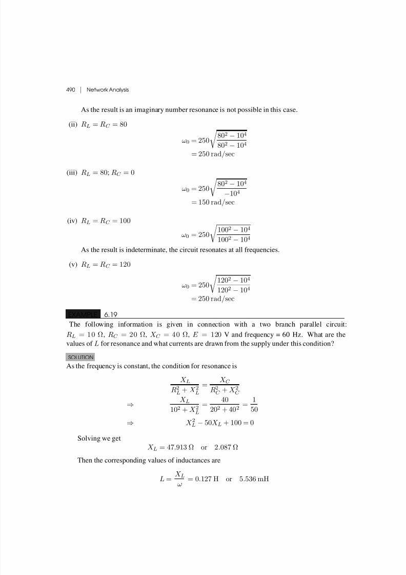
490 | Network Analysis
As the result is an imaginary number resonance is not possible in this case.
(ii) RL = RC = 80
ω0 = 250
802 − 104
802 − 104
= 250 rad/sec
(iii) RL = 80; RC = 0
ω0 = 250
802 − 104
−104
= 150 rad/sec
(iv) RL = RC = 100
ω0 = 250
1002 − 104
1002 − 104
As the result is indeterminate, the circuit resonates at all frequencies.
(v) RL = RC = 120
ω0 = 250
1202 − 104
1202 − 104
= 250 rad/
sec
EXAMPLE 6.19
The following information is given in connection with a two branch parallel circuit:
RL = 1 0 Ω, RC = 2 0 Ω, X C = 4 0 Ω, E = 120 V and frequency = 60 Hz. What are the
values of L for resonance and what currents are drawn from the supply under this condition?
SOLUTION
As the frequency is constant, the condition for resonance is
X LR2
L + X 2
L
= X C R2
C + X 2
C
⇒ X L102 + X 2
L
= 40
202 + 402 = 1
50
⇒ X 2L − 50X L + 100 = 0
Solving we get
X L = 47.913 Ω or 2.087 Ω
Then the corresponding values of inductances are
L = X Lω
= 0.127 H or 5.536 mH

8/12/2019 Unit6-KCV
http://slidepdf.com/reader/full/unit6-kcv 41/44
Resonance | 491
The supply current is
I = EG = E (GL + GC )
Thus, I = 120
10
102 + 47.9132 + 0.02
= 1.7 A for X L = 47.913 Ω
or I = 120
10
102 + 2.0872 + 0.02
= 12.7 A for X L = 2.087 Ω
Exercise Problems
E.P 6.1Refer the circuit shown in Fig. E.P. 6.1, where Ri is the source resistance
(a) Determine the transfer function of the circuit.
(b) Sketch the magnitude plot with Ri = 0 and Ri = 0.
Figure E.P. 6.1
Ans: H (s) = V o (s)
V i (s) =
R
Ls
s2 +R +R i
L
s + 1
LC
E.P 6.2
For the circuit shown in Fig. E.P. 6.2, calculate the following:
(a) f 0, (b) Q, (c) f c1 , (d) f c2 and (e) B
Figure E.P. 6.2
Ans: (a) 254.65 kHz (b) 8 (c) 239.23 kHz (d) 271.06 kHz (e) 31.83 kHz

8/12/2019 Unit6-KCV
http://slidepdf.com/reader/full/unit6-kcv 42/44
492
Network Analysis
E.P 6.3
Refer the circuit shown in Fig. E.P. 6.3, find the output voltage, when (a) = 0 (b)
= 1, and
(c) =
2.
Figure E.P. 6.3
Ans: (a) 640 cos(1.6 106 t)mV(b) 452.55 cos(1.5 106 t + 45 )mV(c) 452.55 cos(1.7 106 t 45 )mV
E.P 6.4
Refer the circuit shown in Fig. E.P. 6.4. Calculate
( ) and then find (a) 0 and (b)
.
Figure E.P. 6.4
Ans: (a) 364.69 krad/sec, (b) 36
E.P 6.5
Refer the circuit shown in Fig. E.P. 6.5. Show that at resonance,
max =
s
1
1
4Q2
.
Figure E.P. 6.5

8/12/2019 Unit6-KCV
http://slidepdf.com/reader/full/unit6-kcv 43/44

8/12/2019 Unit6-KCV
http://slidepdf.com/reader/full/unit6-kcv 44/44
494
Network Analysis
E.P 6.10
A fresher in the devices lab for sake of curiosity sets up a series RLC network as shown in Fig.
E.P.6.10. The capacitor can withstand very high voltages. Is it safe to touch the capacitor at
resonance? Find the voltage across the capacitor.
Figure E.P. 6.10
Ans: Not safe, V
max = 1600V