NASA/TP—2013-217749

August 2013

An Erratum was added to this report March 2014.

Noel N. NemethGlenn Research Center, Cleveland, Ohio

Unit-Sphere Multiaxial Stochastic-Strength ModelApplied to Anisotropic and Composite Materials

NASA STI Program . . . in Profi le

Since its founding, NASA has been dedicated to the advancement of aeronautics and space science. The NASA Scientifi c and Technical Information (STI) program plays a key part in helping NASA maintain this important role.

The NASA STI Program operates under the auspices of the Agency Chief Information Offi cer. It collects, organizes, provides for archiving, and disseminates NASA’s STI. The NASA STI program provides access to the NASA Aeronautics and Space Database and its public interface, the NASA Technical Reports Server, thus providing one of the largest collections of aeronautical and space science STI in the world. Results are published in both non-NASA channels and by NASA in the NASA STI Report Series, which includes the following report types: • TECHNICAL PUBLICATION. Reports of

completed research or a major signifi cant phase of research that present the results of NASA programs and include extensive data or theoretical analysis. Includes compilations of signifi cant scientifi c and technical data and information deemed to be of continuing reference value. NASA counterpart of peer-reviewed formal professional papers but has less stringent limitations on manuscript length and extent of graphic presentations.

• TECHNICAL MEMORANDUM. Scientifi c

and technical fi ndings that are preliminary or of specialized interest, e.g., quick release reports, working papers, and bibliographies that contain minimal annotation. Does not contain extensive analysis.

• CONTRACTOR REPORT. Scientifi c and

technical fi ndings by NASA-sponsored contractors and grantees.

• CONFERENCE PUBLICATION. Collected papers from scientifi c and technical conferences, symposia, seminars, or other meetings sponsored or cosponsored by NASA.

• SPECIAL PUBLICATION. Scientifi c,

technical, or historical information from NASA programs, projects, and missions, often concerned with subjects having substantial public interest.

• TECHNICAL TRANSLATION. English-

language translations of foreign scientifi c and technical material pertinent to NASA’s mission.

Specialized services also include creating custom thesauri, building customized databases, organizing and publishing research results.

For more information about the NASA STI program, see the following:

• Access the NASA STI program home page at http://www.sti.nasa.gov

• E-mail your question to help@sti.nasa.gov • Fax your question to the NASA STI

Information Desk at 443–757–5803 • Phone the NASA STI Information Desk at 443–757–5802 • Write to:

STI Information Desk NASA Center for AeroSpace Information 7115 Standard Drive Hanover, MD 21076–1320

NASA/TP—2013-217749

August 2013

An Erratum was added to this report March 2014.

Noel N. NemethGlenn Research Center, Cleveland, Ohio

Unit-Sphere Multiaxial Stochastic-Strength ModelApplied to Anisotropic and Composite Materials

National Aeronautics andSpace Administration

Glenn Research CenterCleveland, Ohio 44135

Acknowledgments

Available from

NASA Center for Aerospace Information7115 Standard DriveHanover, MD 21076–1320

National Technical Information Service5301 Shawnee Road

Alexandria, VA 22312

Available electronically at http://www.sti.nasa.gov

Level of Review: This material has been technically reviewed by technical management.

The author thanks Dr. John G. Gyekenyesi, Dr. Steven M. Arnold, Dr. Subodh K. Mital, Dr. Osama M. Jadaan,Dr. Robert Goldberg, and Mr. Owen J. Walton for their technical suggestions and assistance. This work

was funded by the NASA Fundamental Aeronautics Program, Supersonics Project.

Trade names and trademarks are used in this report for identifi cation only. Their usage does not constitute an offi cial endorsement, either expressed or implied, by the National Aeronautics and

Space Administration.

This work was sponsored by the Fundamental Aeronautics Program at the NASA Glenn Research Center.

 

NASA/TP—2013-217749 iii

Erratum

Issued March 2014 for

NASA/TP—2013-217749 Unit-Sphere Multiaxial Stochastic-Strength Model Applied to Anisotropic and Composite Materials

Noel N. Nemeth August 2013

Page 6: Equations (12) and (13) should be

cos for 02

02

L

LL

L

  (12)

  

 

0 for 02

sin2 2

for2 2

T

T

TT

T

 

(13) 

                             

NASA/TP—2013-217749 v

Contents Summary........................................................................................................................................................................ 1 1.0  Introduction ............................................................................................................................................................ 1 2.0  Model Description .................................................................................................................................................. 2 

2.1  Unit-Sphere Model for Isotropic Response .................................................................................................... 2 2.2  Unit-Sphere Model Extended for Transversely Isotropic Strength Response ................................................ 5 

2.2.1  Flaw-Orientation Anisotropy ............................................................................................................... 5 2.2.2  Critical Strength or Stress Intensity Factor Anisotropy ....................................................................... 6 

2.3  Failure Modes and Overall Probability of Failure .......................................................................................... 9 2.3.1  Unidirectional Composite Failure Modes .......................................................................................... 10 

3.0  Examples .............................................................................................................................................................. 10 3.1  Application to Nuclear-Grade Graphite ........................................................................................................ 10 3.2  Application to a Unidirectional Polymer Matrix Composite ........................................................................ 12 

3.2.1  Biaxial Failure Envelopes for Three Assumed Models ..................................................................... 17 3.2.2  Model M1: Flaw/Failure Plane Anisotropy ....................................................................................... 17 3.2.3  Model M2: Isotropic Matrix Material ................................................................................................ 20 3.2.4  Model M3: Anisotropic Matrix Material ........................................................................................... 25 

4.0  Summary and Conclusions ................................................................................................................................... 29 Appendix—Symbols ................................................................................................................................................... 31 References ................................................................................................................................................................... 33 

NASA/TP—2013-217749 1

Unit-Sphere Multiaxial Stochastic-Strength Model Applied to Anisotropic and Composite Materials

Noel N. Nemeth

National Aeronautics and Space Administration Glenn Research Center Cleveland, Ohio 44135

Summary

Models that predict the failure probability of brittle materi-als under multiaxial loading have been developed by authors such as Batdorf, Evans, and Matsuo. These “unit-sphere” models assume that the strength-controlling flaws are ran-domly oriented, noninteracting planar microcracks of specified geometry but of variable size. This methodology has been extended to predict the multiaxial stochastic strength response of transversely isotropic brittle materials, including polymer matrix composites (PMCs), by considering (1) flaw-orientation anisotropy, whereby a preexisting microcrack has a higher likelihood of being oriented in one direction over another direction, and (2) critical strength, or KIc orientation anisotropy, whereby the level of critical strength or fracture toughness for mode I crack propagation KIc changes with regard to the orientation of the microstructure. In this report, results from finite element analysis of a fiber-reinforced-matrix unit cell were used with the unit-sphere model to predict the biaxial strength response of a unidirectional PMC previously reported from the World-Wide Failure Exercise. Results for nuclear-grade graphite materials under biaxial loading are also shown for comparison. This effort was successful in predicting the multiaxial strength response for the chosen problems. Findings regarding stress-state interac-tions and failure modes also are provided.

1.0 Introduction The main purpose of this report is to investigate how “unit-

sphere” methodology can be used as a failure criterion inside finite-element- or micromechanics-based software codes for individual brittle (or quasi-brittle) composite-material constit-uents to predict the overall strength response. The term “unit-sphere” as used herein refers to the models that were devel-oped by Batdorf and Crose (1974), Batdorf and Heinisch (1978), Evans (1978), and Matsuo (1981) to predict the probability of failure of brittle materials under multiaxial loading. These models use a unit radius sphere representing the random orientation of flaws to calculate the effect of multiaxial stresses on material reliability. This approach assumes that the strength-controlling flaws are randomly oriented, noninteracting planar microcracks of specified geometry but of variable size. Fracture mechanics relation-

ships for mixed-mode (modes I, II, and III) crack growth, combined with the weakest-link theory and integration over the surface area of a unit radius sphere representing all possible orientations of microcracks, are used to calculate the material probability of failure. This unit-sphere methodology was originally introduced within a statistical theory of brittle material strength by Weibull (1939), though without consider-ation for the mechanics of crack growth.

This report describes the development of the unit-sphere methodology for generalized anisotropic strength response (in this case, for transverse isotropy) and the use of the methodology to predict the biaxial strength response of a unidirectional polymer matrix composite (PMC) previously reported from the World-Wide Failure Exercise (WWFE) from Hinton et al. (2004). Also shown are results for nuclear-grade graphite materials under biaxial loading. These two examples represent an application to a homogeneous material (i.e., graphite) and a heterogeneous material system (i.e., a fiber-reinforced composite) under multiaxial loading. A follow-on phase of this effort, not described here, allows this technology to work with NASA’s MAC/GMC micromechanics analysis code (MAC) of Bednarcyk and Arnold (2002), which is based on the generalized method of cells (GMC) family of micromechanics theories, including doubly and triply periodic versions of the GMC (Aboudi (1995)) and the High-Fidelity Generalized Method of Cells (HFGMC) (Aboudi et al. (2003)). This incorporation will allow the full exercise of the unit-sphere methodology, including incremental time/load steps and fatigue analysis (as described in Nemeth et al. (2005)), to predict the durability (strength and lifetime) of composite laminates and woven composite structures.

Central to this report is the assumption that a composite material is controlled by various independent failure modes and that these failure modes follow a Weibull distribution. The product of the probability of survival of the various failure modes yields the probability of survival (the reliability) of the composite. This is a weakest-link assumption. The weakest-link theory (WLT) and the Weibull distribution predict a size effect (whereby larger components have a lower average strength than equally loaded smaller components). Size-effect studies are often used by researchers as a proxy to test WLT behavior and the applicability of the Weibull strength theory for a material.

The review article by Wisnom (1999) examines the then-available experimental data for PMCs regarding size effect

NASA/TP—2013-217749 2

and Weibull distribution for various composite failure modes. Various defect populations and factors that influence the size effect are discussed, as are the strengths and weaknesses of the Weibull approach. Wisnom (1999) indicated that there was broad evidence from the literature for size effects for all failure modes, although there were also inconsistencies and complications in the experimental record. Generally Wisnom (1999) concluded that the size effect was consistent with a Weibull modulus between 13 and 29 and that size effect was larger for matrix-dominated failure, for which the experi-mental data correlated reasonably well with the trend pre-dicted by the Weibull strength theory. For ceramic matrix composites (CMCs), size effect has been studied by others—for example, Calard and Lamon (2002), Lamon (2001), and Nozawa et al. (2002), although the experimental record is relatively meager in comparison to that for PMCs. These papers are just a few noteworthy examples from the literature on the subject of size effect and strength scatter in composites.

It is clear that the phenomenon of damage accumulation and interaction, as opposed to standard WLT, complicates the situation regarding size effect. However, by focusing instead on the failure behavior of the individual composite material constituents of fiber and matrix (and interface or interphase), which by themselves are brittle or quasibrittle monolithic materials, the application of the Weibull distribution to describe damage initiation appears to be a more straightforward and reasonable exercise. Indeed this approach was taken by Guillaumat and Lamon (1996) and by Lamon et al. (1998) for their simulations of the matrix damage evolution of a woven CMC using their isotropic strength response unit-sphere model. For fiber (bundle) strength modeling in a PMC, Harlow and Phoenix (1978) indicate that WLT is an operative mechanism and that the strength distribution is approximately Weibull within the probability range of interest. This argument is also supported by Mahesh et al. (1999, 2002), Mahesh and Phoenix (2004), and Landis et al. (2000). The review article(s) by Nemeth and Bratton (2010, 2011) discuss in more detail some of the theoretical work and simulations that others have per-formed regarding strength scatter and size effect in composites.

In this report, the unit-sphere methodology is described first for an isotropic material strength response followed by the modeling needed to enable the prediction of strength response for a transversely isotropic material in fast fracture (which is the intrinsic material strength without regard to time- or cycle-dependent strength degradation). These extensions are for (1) flaw-orientation anisotropy, whereby a preexisting micro-crack has a higher likelihood of being oriented in one direction over another direction, and (2) critical strength or fracture toughness anisotropy, whereby the level of critical strength Ic or fracture toughness KIc for mode I crack propagation changes with the orientation of the microstructure (for a

tensile mode of failure only). These modeling extensions are then demonstrated for a (macroscopically) homogeneous material—in this case, nuclear-grade graphite—followed by an application to a heterogeneous material—a unidirectional glass/epoxy PMC. Only biaxial tension/compression loading was considered here. The intent is to show the progression of the model from a homogeneous isotropic material, to a homo-geneous anisotropic material, and then to a heterogeneous anisotropic composite material. This includes illustrating the consequence of shear sensitivity, global fracture planes, and failure modes on multiaxial strength.

The unit-sphere methodology is an attempt to provide a mechanistic basis to the problem of predicting the strength response of a composite under multiaxial loading that is improved in comparison to polynomial interaction equation formulations such as Tsai-Wu, Tsai-Hill, and Hashin, among others. The unit-sphere methodology is not a true physics-based simulation whereby cracks nucleate or initiate from preexisting flaws, grow, and interact to progressively damage the material. However, those methods are computationally intensive and do not establish the statistics of failure without further considera-tion of the size distribution, the spatial distribution, and the orientation biases of inherent source flaws or defects.

2.0 Model Description 2.1 Unit-Sphere Model for Isotropic

Response In the Batdorf unit-sphere theory, the incremental failure

probability PfV under an applied multiaxial state of stress at a given location in the component can be described as the product of two probabilities:

VVeqcfV PPVP 21I ,, (1)

where P1V is the probability of the existence in the volume V of a crack having an equivalent critical strength between Ieqc and Ieqc + Ieqc. Critical strength Ic is defined as the remote, uniaxial fracture strength of a given crack in pure mode I loading. The term Ieqc denotes an effective (or equivalent) critical mode I stress from applied multiaxial stresses. The second probability, P2V, denotes the probability that a crack with critical strengthIeqc will be oriented in a direction such that an effective stress Ieq (which is a function of fracture criterion, stress state, and crack configuration) satisfies the condition Ieq Ieqc. An incremental volume V is used in Equation (1) because an infinitesimal volume dV cannot enclose a crack of critical strengthIeqc and associated critical crack length of ac.

NASA/TP—2013-217749 3

The effective stress Ieq represents an equivalent normal stress on the crack face from the combined action of the normal stress n and the shear stress . The microcrack orientation is defined by the angular coordinates, and , where the direction normal to the plane of the microcrack is specified by the radial line defined by and (see Fig. 1(b)). For the sake of brevity, the development of the effective stress equations is not shown (for details, see Nemeth et al. (2003, 2005)). For a penny-shaped crack with the Shetty mixed-mode fracture criterion (Shetty (1987)), the effective stress becomes

2

2I

1 4 2 2

eq n nC

(2)

where is Poisson’s ratio and C is the Shetty shear-sensitivity coefficient, with values typically in the range 0.80 ≤ C ≤ 2.0. As C increases, the response becomes progressively more shear insensitive. Shear increases the equivalent stress as shown in Equation (2), and this has a deleterious effect on the predicted material strength. For a penny-shaped crack with a material having a Poisson’s ratio of about 0.22 and C = 0.80, 0.85, 1.05, and 1.10; Equation (2) approximates, respectively, the following criteria: Ichikawa’s maximum energy-release-rate approximation (Ichikawa (1991)), the maximum tangential stress (Erdogan and Sih (1963)), Hellen and Blackburn’s (1975) maximum strain-energy-release-rate formulation, and colinear crack extension. The value of C also can be fit empirically to experimental data—either on introduced cracks (as was done in Shetty (1987)) or on specimens being tested multiaxially.

The strength of a component containing a flaw population is related to the critical flaw size, which is implicitly used in Batdorf’s theory. Batdorf and Crose (1974) describe P1V as

I1 I

I

dd

dV eqc

V eqceqc

P V

(3)

and P2V is expressed as

4,

I2

eqcVP (4)

where V(Ieqc) is the Batdorf crack-density function and (, Ieqc) is the area of the solid angle projected onto the unit radius sphere in stress space (see Fig. 1) containing all the crack orientations for which Ieq ≥ Ieqc for the applied far-field multiaxial stress state . The infinitesimal area, dA, on the unit sphere represents a particular flaw orientation (a direction normal to the flaw plane), and Ieq is an equivalent, or effective, stress, which is a function of an assumed crack shape

Figure 1.—Projection of equivalent stress onto a unit radius

sphere. (a) Cauchy stress components on an infinitesimal tetrahedron resolving a normal stress, n, and a resultant shear stress, , on a plane normal to the direction defined by angular coordinates and . (b) Projection of equivalent stress onto a unit radius sphere in the global coordinate system. The unit radius sphere represents all possible flaw orientations, where Ieq is an equivalent (or an effective) stress, x, y, and z are normal orthogonal stress compo-nents, and xy, yz, and zx are shear stress components. An infinitesimal area, dA, on the unit sphere represents a particular flaw orientation (a direction normal to the flaw plane), and Ieq is a function of an assumed crack shape and multiaxial fracture criterion.

NASA/TP—2013-217749 4

and multiaxial fracture criterion. The constant 4 is the surface area of a unit radius sphere and corresponds to a solid angle containing all possible flaw orientations.

The probability of failure for the arbitrarily loaded volume V is

I ,max I I

0 I

, d1 exp d

4 deq eqc v eqc

fVV eqc

P V

(5)

where Ieq,max is the maximum effective stress that a flaw could experience from the given stress state and for all possible flaw orientations. The crack-density function V(Ieqc) is independent of the stress state and has been approximated by a power function (Batdorf and Heinisch (1978)). This leads to the Batdorf crack-density function of the form

V

V

moV

meqcBV

eqcVk

),,z,y,x( I

I (6)

where x, y, and z correspond to the location, and are orientation angles, mV is the shape parameter, and BVk is the normalized Batdorf crack-density coefficient.

The scale parameter oV corresponds to the stress level where 63.21 percent of tensile specimens with unit volumes would fracture. A similar quantity, the characteristic strength V, is the stress level (which is the peak stress for a nonuni-formly stressed specimen—such as a specimen undergoing four-point bending) at which 63.21 percent of specimens fail. The characteristic strength is functionally related to the scale parameter by 1 Vm

V oV eV as explained in other publica-tions, such as Nemeth et al. (2003, 2005). The effective volume Ve is an equivalent amount of volume under uniform loading (with no stress gradients) that produces the same probability of failure as a specimen of volume V under loading where stress gradients may or may not be present. For a pure tensile specimen where stress distribution is uniform in the gauge section, the effective volume is equivalent to the volume of the gauge section. When stress gradients are present, a more complicated integral relationship is required to determine Ve (Nemeth et al. (2003, 2005)).

The scale parameter oV has dimensions of stress (volume) 1/ ,Vm where mV is the shape parameter (Weibull modu-lus)—a dimensionless parameter that measures the degree of strength variability. As mV increases, the dispersion decreases.

The normalized Batdorf crack-density coefficient BVk is a function of the microcrack geometry and mixed-mode fracture criterion chosen. The value of BVk normalizes Equation (5) to the two-parameter Weibull equation for a uniaxial stress state (see Nemeth et al. (2003, 2005)). It also means that Equation (5) takes on the characteristics of a two-parameter Weibull distribution. The Weibull distribution is obtained if the defect size distribution is described by a power law. A Gumbel-type extreme-value distribution should be obtained if the defect size is exponentially distributed. Typically brittle material strength is described with the Weibull distribution. The normalized Batdorf crack-density coefficient ,BVk the scale parameter oV, and the Weibull modulus mV are evaluated from experimental inert strength (fast-fracture) data of specimens.

To determine the probability of failure over V, one must evaluate P2V (in Eq. (5)) for each elemental volume Vi within which a uniform multiaxial stress state is assumed. The solid angle (, Ieqc) depends on the selected fracture criterion, the crack configuration, and the applied stress state. For multiaxial stress states, with few exceptions, (, Ieqc) must be deter-mined numerically. Fortran was used to develop the unit-sphere numerical algorithms for this work.

For a sphere of unit radius (see Fig. 1), an elemental surface area of the sphere is dA = sin d d. If we project onto the spherical surface the equivalent (effective) stress Ieq(, , ), the solid angle (, Ieqc) will be the area of the unit sphere containing all the projected equivalent stresses satisfying Ieq ≥ Ieqc. Because of the symmetry of the stresses, this integration can be performed over one-half of the sphere (0 /2); therefore,

2

0

2

0II

I ddsin ,21

4,

eqceqeqc H (7)

where

eqceqeqceq

eqceqeqceq

H

H

IIII

IIII

0 ,

1 ,

and H is the Heaviside function. Substituting Equations (6) and (7) into Equation (5) and integrating with respect to Ieqc results in (see Batdorf (1978a,b) and Nemeth et al. (2003, 2005)):

V

m

oV

eqBVfV VkP

V

d ddsin ,,z,y,x(

2

exp 1 2

0

2

0

I (8)

NASA/TP—2013-217749 5

For a given incremental volume, Ieq(x, y, z, , ) is the projected equivalent stress over the unit radius sphere in stress space as depicted in Figure 1. Using the power-law crack-density function V of Equation (6) will characterize the Batdorf model in Equation (8) as a form of the Weibull distribution. Equation (8) circumvents the more involved numerical integration of (, Ieqc).

It should be mentioned that, in the numerical implementation of Equation (8) when n becomes compressive, its value is set to zero in Equation (2) and is adjusted by subtracting the absolute value of n from it. This happens when the absolute value of (n/) 0.5 in the algorithm so that the adjusted value of is never allowed to be less than zero. When the absolute value of (n/) 0.5 (which was a somewhat arbitrarily set value from trial and error experience), then Ieq is set to zero. These conditions are imposed to avoid an abrupt transition so that, when n goes from tension to compression, there will never be a failure of the flaw (regardless of the value of ). By subtracting the absolute value of n from , the effective stress Ieq is reduced. This provides a penalty (in a simplistic way) for the effect of friction on the crack face by increasing the resistance to mode II and III failure. This was found to be a practical way to avoid abrupt transitions in failure probability tendencies when going from tensile to compressive loading (such as seeing discontinuities in failure envelopes when contour lines of constant probability of failure are being plotted).

2.2 Unit-Sphere Model Extended for Trans-versely Isotropic Strength Response

Two different physical mechanisms were considered in order to extend the unit-sphere model to account for aniso-tropic strength response: (1) flaw-orientation anisotropy, whereby a preexisting microcrack has a higher likelihood of being oriented in one direction over another direction, and (2) critical strength or fracture toughness anisotropy, whereby the level of critical strength Ic or fracture toughness KIc for mode I crack propagation changes with regard to the orienta-tion of the microstructure (for a tensile mode of failure only in this case). Flaw-orientation anisotropy was previously consid-ered by Buch et al. (1977), and critical strength anisotropy was previously considered by Batdorf (1973). Both models were developed to model monolithic graphite anisotropic strength response. Extensions to these models are described herein for a transversely isotropic strength response. The extensions include shear sensitivity for flaws, an improved functional form for the anisotropy equations, and consideration of multiple failure modes. A corollary of the unit-sphere model is

that the probability density distribution of the orientation of critical flaws in a multiaxial stress state can be obtained. This is described separately in Nemeth (2013).

2.2.1 Flaw-Orientation Anisotropy Flaw-orientation anisotropy refers to the situation where a

flaw has a higher likelihood of being oriented in one direction than another for a given critical strength. Thus, a material will be stronger on average in one direction than another. An isotropic brittle material is equally strong in any direction, and thus its flaws are uniformly randomly oriented. However, for components made by processes such as extrusion or hot-pressing, which induce texture, a bias will exist in the orienta-tion distribution of processing flaws. Also, components finished by surface grinding will contain machining damage in the form of surface cracks that are oriented parallel and transverse to the grinding direction. For composite materials, the interface, or an interfacial layer between the fiber and the matrix, can act as a flaw with an orientation bias that induces an anisotropic strength response.

For volume-distributed flaws, flaw-orientation anisotropy relative to a material coordinate system is modeled by intro-ducing a probability density distribution into the unit-sphere formulation (see Buch et al. (1977). Then for P2V in Equation (4),

2

0

2

0II2 ddsin ,, eqceqV HP (9)

where

2

0

2

0ddsin ,

),(),( (10)

and

I I I I

I I I I

, 1

, 0

eq eqc eq eqc

eq eqc eq eqc

H

H

The term (, ) d dβ denotes the probability that a crack of critical strengthIeqc is oriented in the range between α and ( + d) and between β and (β + dβ), where the orientation of the microcrack is described by the vector that is normal to the plane of the microcrack. The function () describes the degree of anisotropy of flaw orientation, where the normal direction to the flaw plane is given by angles and .

NASA/TP—2013-217749 6

Equations (9) and (10) modify Equation (8) for probability of failure as

where the normalized crack-density coefficient BVk is evaluated numerically for a uniaxial stress state applied in one of the material coordinate system axis directions.

For a transversely isotropic strength response, ζ in Equation (10) is only a function of α. Buch et al. (1977) introduced a cosine power function for ζ(α) = [cos (α)]φ where φ is a constant. This relation is modified herein to enhance the functional flexibility:

( )

( )

cos for 02

02

L

LL

L

φ απ ς α = ≤ α ≤ Λ Λ π ς α = Λ <

(12)

Alternatively,

( )

( )

0 for 02

sin2 2

for2 2

L

T

TL

T

φ

π ς α = ≤ α < −Λ

π π ς α = α − −Λ Λ π π−Λ ≤ α ≤

(13)

where Λ and φ are constants (with subscripts L or T) that control the degree of anisotropy, and 0 < Λ ≤ π/2 and φ ≥ 0. When Λ = π/2 and φ = 0, an isotropic strength response is obtained. Equations (12) and (13) are defined for one-half of the unit sphere (the top half is as shown in Fig. 1, where 0 ≤ α ≤ π/2). Referring to Figure 2, Equation (12) represents the “polar-cap,” or longitudinal, L distribution of flaws and Equation (13) represents an “equatorial-belt,” or transverse, T distribution of flaws. The polar-cap distribution describes crack planes symmetrically distributed (centered) about a plane (in this case the σy−σz plane), and the equatorial-belt distribution describes crack planes symmetrically distributed (centered) along a line (in this case, the σx axis). For the polar-cap distribution, BVk is evaluated for a uniaxial stress

along the σx direction; and for the equatorial-belt distribution, it is evaluated in the σy (or optionally the σz) direction.

The separate polar-cap and equatorial-belt distributions are introduced to describe individual, and distinctly different, failure modes. For a unidirectional fiber-reinforced composite, the polar cap can be used to represent the fiber strength distribution and the equatorial belt can be used to represent the matrix-fiber interface. The equatorial-belt and the polar-cap distributions can be considered to equivalently represent global failure planes, which are referred to as “action planes” in the Puck multiaxial strength model for composites (see Lutz (2006) for a description). The angular width of the belt or cap with regard to angle α indicates the maximum extent of scatter of a flaw orientation. Flaws or action planes oriented outside of the scatter bands of the cap and belt are assumed not to exist or to not contribute to the likelihood of failure.

2.2.2 Critical Strength or Stress Intensity Factor Anisotropy

Batdorf (1973) approached strength anisotropy using the σIc strength ellipsoid approach (describing an ellipsoid rather than a unit sphere). In this report, strength anisotropy is used with the critical stress intensity factor (fracture toughness) KIc varying with the orientation angle on the unit sphere. This is functionally equivalent to σIc varying with orientation, and it is also functionally equivalent to the size of the flaw changing with the orientation angle. For a CMC, where failure from loading in the fiber direction is by matrix cracking with large-scale fiber bridging, fracture toughness cannot be defined on the global scale of the structure. In that case, one has to alternatively consider critical strength as a metric. However, it is acceptable to use fracture toughness on the local scale at the crack tip, where micromechanics can account for the bridging explicitly. In this report, fiber bridging is not considered directly. Of first-order importance herein is that the local fracture toughness could change with the orientation of the flaw plane (or action plane) and the applied loading. The specific micromechanics of how this might occur is not considered here.

The modeling approach taken here is similar to that described previously for flaw-orientation anisotropy. The criti-cal strength σIc is defined as the fracture strength of the crack in mode I loading and is proportional to KIc. Therefore, for anisotropic KIc(α, β) = (c σIc(α, β)) = ( )],[ Imax,I βασ cc fc , where

(11)

NASA/TP—2013-217749 7

Figure 2.—Unit sphere with probability density distribution functions (PDFs) describing the anisotropy of the flaw

orientation, where and are angular coordinates and L and T are constants in the flaw-orientation aniso-tropy function representing longitudinal and transverse distributions. Orientation is described with the normal to the crack plane. In this figure, two orientation functions are described: (1) a polar-cap distribution (Eq. (12)) describing crack planes symmetrically distributed (centered) about a plane (in this case the y–z stress plane) and (2) an equatorial-belt distribution (Eq. 13)) where crack planes are symmetrically distributed (cen-tered) along a line (in this case the x axis).

c is a constant ( caYc with crack-shape geometry factor Y and critical crack length ac), Ic,max is the maximum value of Ic over the unit sphere (for all and ), and I ,cf is a normalized function expressing the degree of this anisotropy. The unit-sphere formulation described previously is used, except the Heaviside step function in Equations (7) and (10) is modified as follows

max,II

II

max,II

II

,

0 ,

,

1 ,

eqcIc

eqeqceq

eqcIc

eqeqceq

fH

f

H

(14)

NASA/TP—2013-217749 8

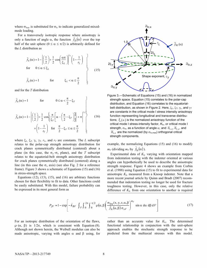
where Ieqc is substituted for Ic to indicate generalized mixed-mode loading.

For a transversely isotropic response where anisotropy is only a function of angle , the function Icf over the top half of the unit sphere (0 /2) is arbitrarily defined for the L distribution as

2for1)(

0for

11cos21

211)(

I

I

Lc

L

LLc

f

rf

L

(15)

and for the T distribution

22for11

2cos

21

211)(

20for1)(

I

I

TT

TT

c

Tc

r

f

f

T

(16)

where L, T, L, T, rL, and rT are constants. The L subscript relates to the polar-cap strength anisotropy distribution for crack planes symmetrically distributed (centered) about a plane (in this case, the yz plane), and the T subscript relates to the equatorial-belt strength anisotropy distribution for crack planes symmetrically distributed (centered) along a line (in this case the x axis) (see also Fig. 2 for a reference frame). Figure 3 shows a schematic of Equations (15) and (16) in stress-strength space.

Equations (12), (13), (15), and (16) are arbitrary functions chosen for their flexibility to fit to data. Other functions could be easily substituted. With this model, failure probability can be expressed in its most general form as

For an isotropic distribution of the orientation of the flaws, (, ) is 1/2, which is consistent with Equation (8). Although not shown herein, the Weibull modulus can also be made anisotropic, varying with angles and using, for

Figure 3.—Schematic of Equations (15) and (16) in normalized

strength space. Equation (15) correlates to the polar-cap distribution, and Equation (16) correlates to the equatorial-belt distribution, as shown in Figure 2. Here, L, T, L, and T are constants in the critical mode I stress intensity anisotropy function representing longitudinal and transverse distribu-tions; cfI is the normalized anisotropy function of the critical mode I stress-intensity factor, KIc, or critical mode I strength, Ic, as a function of angle and ,, y,Ix,I cc and

z,Ic are the normalized (by Ic,max) orthogonal critical

strength components. example, the normalizing Equations (15) and (16) to modify mV (dividing mV by cfI ).

Experimental data of KIc varying with orientation mapped from indentation testing with the indenter oriented at various angles can hypothetically be used to describe the anisotropic strength response. Figure 4 shows an example from Corbin et al. (1988) using Equation (15) to fit to experimental data for anisotropic KIc measured from a Knoop indenter. Note that a more recent journal article by Quinn and Bradt (2007) recom-mended that indentation testing no longer be used for fracture toughness testing. However, in this case, only the relative difference of KIc from one orientation to another is required

rather than an accurate value for KIc. The determined functional relationship in conjunction with the unit-sphere approach enables the stochastic strength response to be predicted from the multiaxial stresses with this model.

(17)

NASA/TP—2013-217749 9

Figure 4.—Indentation testing used to determine the relation-

ship between the critical mode I stress intensity factor, KIc, and the whisker axis direction. Here the constants in the KIc anisotropy function representing the longitudinal distribu- tion are L = /2 radians (90), L = 1.0, and rL = 1.23 from Equation (15), and is an angular coordinate. Experimental results from Corbin et al. (1988).

Alternatively, specimens could be cut at various angles to a given direction in order to obtain strength properties. From that information, the necessary functional relationship of strength with angle would also be obtained for model calibration.

2.3 Failure Modes and Overall Probability of Failure

A material is assumed to have n individual failure modes. Material reliability (probability of survival Ps where Ps = 1 – Pf) is assumed to be the product of the survival probability of all of the failure modes:

is

n

is PP ,

1

(18)

where each failure mode (denoted with the subscript i) has its own unique failure criterion and parameter description. For an isotropic material volume, two failure modes can be assumed: one for tensile failure and the other for compressive failure. The tensile-failure mode is described by Equation (8) and the effective stress relation of Equation (2). The compressive-failure criterion is assumed to be of a different nature than the tensile-failure mode—possibly involving the interaction of arrested cracks (flaws with initial crack growth that subse-quently stops because of the angle of the crack growth and the interaction with the local stress field). Regardless, the Weibull distribution is assumed to describe the stochastic strength response phenomenologically. This is argued further in Nemeth and Bratton (2011) on the basis of the statistical uncertainty in experimental data and a simple version of Freudenthal’s (1968) uniform defect model (Nemeth and Bratton (2011), App. A). The compressive-failure mode is assumed to be controlled by shear stress, and a simple Tresca-like effective stress relation can be prescribed:

Ieq = 2 (19)

The multiplier of 2 in Equation (19) is chosen so that the maximum effective stress on the unit sphere in pure uniaxial compression is equal to the applied compressive stress. When the normal stress component n on the crack face is tensile, then the value of Ieq in Equation (19) is set to zero. In this manner, the integration about the unit sphere in Equation (8) proceeds. This methodology can be used with the flaw-orientation anisotropy model of Equations (9) to (13). However, a version analogous to the critical strength anisotropy model of Equations (14) to (17) has not been developed. Therefore, for this report, an isotropic strength response was assumed with this failure mode, unless it was specifically stated that flaw-orientation anisotropy was also used with this model.

Modeling compressive failure with a Weibull distribution is a phenomenological assumption here. Scatter in strength can be substantial in compression as exemplified in Kittl and Aldunate (1983) for over 500 cement cylinders. They found that the normal, lognormal, and three-parameter Weibull distribution could not be chosen conclusively over each other as the best fit to the data. In a more rigorous treatment, Alpa (1984) extended the Batdorf unit-sphere methodology to account for compression by including the frictional effects of the opposed crack surfaces in contact for the multiaxial loading of an isotropic brittle material. Alpa’s treatment required that the Weibull modulus in tension and compression were the same. Here, failure in compression is treated as a separate failure mode, which allows the Weibull modulus for the compressive strength response to be different than the

NASA/TP—2013-217749 10

Weibull modulus in tension. Puck and Shurmann (1998) (as well as Pinho et al. (2005)) consider frictional effects in their solution of the fracture plane.

Multiaxial strength models are typically calibrated to exper-imental rupture data for simple loadings representing particu-lar failure modes, such as uniaxial tension and uniaxial compression. Specimen geometries such as cylinders, beams, or circular disks loaded in tension, flexure, or compression are usually used, and repeats of each test are required in order to obtain the fracture statistics (and hence, the Weibull param-eters). For an isotropic material, stochastic strength data in tension and compression can be obtained without regard to orientation relative to a material axis.

2.3.1 Unidirectional Composite Failure Modes

For an anisotropic material, stochastic strength data must be obtained relative to the different material axes. For a unidirec-tional PMC or CMC, this means strength testing in tension and compression for loadings parallel and transverse to the fiber direction as well as shear testing parallel and transverse to the fiber direction. Four failure modes are assumed herein for a unidirectional composite: (1) fiber fracture failure mode in longitudinal tension (loading in the fiber direction), (2) failure from longitudinal compression, (3) failure from transverse tension (loading perpendicular to the fiber direction), and (4) failure from transverse compression loading. These are assumed to be noninteracting competing failure modes possibly confined (or coalescing) along specific macroscopic fracture planes. This approach is consistent with Puck’s theory that the failure of a composite is controlled or confined to various action planes.

Tensile and compressive rupture loadings are used to esti-mate Weibull parameters, whereas shear loadings help to establish .C Failure from pure shear loading is not considered to be a separate failure mode here because it is coupled to tensile failure by the assumption that the same flaws that control the tensile-failure response also control the shear strength failure response. This is indicated in Equation (2), where mixed-mode loadings are coupled through an effective stress relation. This also implies that the Weibull modulus in transverse tension and shear loading (both matrix-controlled failure modes) are the same. However, in the PMC review by Wisnom (1999), the Weibull modulus seems to be larger in shear tests than for matrix transverse tension. It was not clear whether or not this was an artifact of the testing and the complex failure mode that results. Regardless, the assumption that shear mode failure has the same Weibull modulus of the matrix transverse tension failure mode is conservative.

For transverse compression, the shear loading on the unfavorably oriented flaws in the matrix are assumed to drive the failure response (see Eq. (19)). This is allowed herein to be a phenomenologically different failure mode from the tensile-failure mode of Equation (2). The Weibull modulus can

therefore be different from that of the matrix tensile-failure mode as discussed in Section 2.3.

Failure from transverse tension and failure from transverse compression loading are assumed to be matrix-controlled failure modes. This is handled by the unit-sphere model as described in Section 2.0. The fiber fracture failure mode for the fiber bundle is also assumed to behave in an approximately Weibull manner as discussed in Section 1.0. Here the same unit-sphere model will be used; however, fiber fracture will be assumed to be confined (or localized) to a specific fracture plane normal to the fiber (the polar-cap distribution as shown in Fig. 2). This essentially means that fibers are assumed to fail only by uniaxial tensile loading. This is not to say that a more general three-dimensional unit-sphere model could be used here to account for multiaxial loading and possible strength anisotropy in the fiber. However, for the demonstra-tion problem that follows, this simplified failure criterion suffices. For PMCs, the review by Wisnom (1999) indicates that there is a clear size effect in the matrix for transverse tensile loading consistent with the Weibull theory.

For the failure mode resulting from uniaxial compressive loading along the fiber axis (longitudinal loading), another simple criterion is assumed. In this case, failure of the compo-site occurs when the longitudinal compressive stress in the fiber exceeds a critical value. This critical value is assumed to be Weibull distributed. This criterion is provided here only so that closed failure envelopes can be shown. Failure from longitudinal compression is an area where research and model development is still evolving. It involves mechanisms such as microbuckling and fiber kinking. These are topics beyond the scope of this report. Pinho et al. (2005) provide a good overview and review of this topic. The review by Wisnom (1999) for PMCs does cite evidence for a size effect for this mode of loading, although the few studies performed made drawing firm conclusions difficult.

3.0 Examples In the two examples that follow for nuclear-grade graphite

and a unidirectional PMC, probability-of-failure strength envelopes were made for various combinations of biaxial loading. The nuclear-grade graphite material is treated as a continuum, whereas the PMC is a heterogeneous material system that requires the determination of the individual constituent micromechanical stress fields. The nuclear-grade graphite example is included to show the effect of shear sensitivity on flaws in comparison to its effect on unidirec-tional PMCs.

3.1 Application to Nuclear-Grade Graphite Figure 5 presents the predicted biaxial failure envelopes for a

near isotropic IG–110 (Sookdeo et al. (2008)) and transversely

NASA/TP—2013-217749 11

isotropic H–451 (Burchell et al. (2007)) nuclear-grade graph-ites. Testing was performed on axially loaded and internally pressurized thick-walled hollow graphite cylinders. This imparted controlled axial and hoop stresses in the specimen gauge volumes. The manufacturing process produced a mild strength anisotropy in the IG–110 graphite billets and a stronger anisotropic response in the H–451 billets. The cylindrical specimens were cut from the billet stock so that axial specimen

loading tested the stronger material direction and that hoop stresses from the internal pressurization tested the weaker material direction. Two separate failure modes for tension and compression were assumed, and the Weibull parameters used in the modeling were calibrated as such. Multiaxial strength response and the effect of the shear sensitivity parameter C (Eq. (2)) on the natural flaws were predicted.

Figure 5.—Example of predicted biaxial failure envelopes for a near isotropic and

transversely isotropic nuclear-grade graphite. Two separate failure modes for tension and compression were assumed. The envelope of the predicted effect of the shear sensitivity parameter C (Eq. (2)) on the natural flaws is shown (with C ranging between 0.82 and 100). (a) Isotropic strength response predicted for 50-percent probability of failure, Pf, for IG–110 grade graphite (Sookdeo et al. (2008)). (b) Transversely isotropic strength response predicted for H–451 graphite (Burchell et al. (2007)) for various failure probabilities and values of C .

NASA/TP—2013-217749 12

Figure 5(a) shows the predicted 50-percent probability-of-failure response for IG–110 grade graphite, where it was assumed that the strength behavior was isotropic (the actual material behavior was near isotropic). For the tensile response, the employed parameters are mV = 22.43, V = 26.38, and = 0.22 (assumed), and C ranges from 0.82 to 100. Note that oV is not specifically needed here because the stress state in the gauge section can be considered to be uniform. For the compressive response, mCV = 22.43 and CV = 81.32 MPa were assumed because there were no available compressive strength data (subscript C denotes the compressive failure mode). A strongly shear-sensitive response was imposed with C = 0.82, and a shear insensitive response was imposed with C = 100. The model correlated best to the experimental data for C 1.2, indicating a moderate shear sensitivity on the flaws. It should be mentioned that values for the Batdorf crack-density coefficient BVk are generally not provided in this report. These values are numerically calculated within the software from the experimental data and do not require any specific treatment by the user. This parameter is described further in Nemeth et al. (2003, 2005).

Figure 5(b) models a transversely isotropic strength response for H–451 graphite, showing C ranging between 0.82 and 100 and various failure probabilities. Anisotropy of KIc with flaw orientation was assumed. For the tensile response, the parameters are mV = 6.58 and V = 17.05 MPa in the axial direction, with = 0.22. In the hoop direction, a char-acteristic tensile strength response of V = 11.01 MPa was modeled, where the parameters for the equatorial-belt distribution in Equation (16) were T = 1.571 radians (90o), T = 1.0, and ( C = 0.82; rT = 2.323), (C = 1.4; rT = 1.915), and (C = 100; rT = 1.708). The values for factor rT were found using a simple interval halving search algorithm for a user-specified level of failure probability and multiaxial stress state. The values for the parameters T = 1.571 radians (90o) and T = 1.0 were arbitrarily chosen on the basis of an assumption that the variation of KIc with orientation was gradual—not abrupt. This approach is consistent with that of Figure 4 from the results of Corbin et al. (1988) for an extruded silicon-nitride/silicon-carbide whisker system. For the H–451 graphite, no information was available on the variation of KIc with orientation nor was it known if (and to what degree) anisotropic residual stresses were present in this batch of material. However, the assumption that KIc would not vary abruptly with orientation appears to be reasonable. For the compressive strength response, mCV = 12.29 and CV = 54.39 MPa. An isotropic compressive strength response was assumed because there were no available compressive strength rupture data in the hoop direction. Also, as previously mentioned, an anisotropic version of this failure criterion for

critical strength has not been developed. From Figure 5(b) the model that correlated best to the experimental data was for

1.4,C again indicating a moderate shear sensitivity on the flaws.

Figure 5(a) is shown mainly for illustrative purposes. Models of H–451 graphite assuming flaw-orientation aniso-tropy (Equations (9) to (13)) or that an anisotropic residual compressive stress was present were not attempted here. Nemeth et al. (2012) showed that the trends observed in the fracture data of an extruded H–451 graphite log (data from Price (1976)) were consistent with an anisotropic compressive residual stress component. However, any physical evidence to further support that conjecture was not available.

It can be seen in both Figure 5(a) and (b) that the shear sensitivity on the flaws primarily affects quadrants two and four (the tension-compression quadrants) for the tensile-failure model using Equation (2). The effect of C on the first (tension-tension) quadrant is small and would be difficult to detect from experimental data. The failure envelope in Figure 5(a) for compressive loadings is qualitatively compara-ble to those of Alpa (1984). Although not shown, there are transition regions present where one failure mode becomes more dominant over the other.

It should be noted that, although it is true that the param-eters of the model were tuned to the graphite data, the aniso-tropy parameters themselves do have physical meanings and they could, hypothetically, be tested independently. Also the model could be tested against other multiaxial loading scenar-ios. The fact that the model worked well in this case indicates that the modeling approach is viable.

3.2 Application to a Unidirectional Polymer Matrix Composite

The biaxial strength response for a PMC was predicted from the strength response of the individual material constituents. In order to achieve this, a finite element analysis (FEA) of a square-packed fiber-in-matrix unit cell was used to obtain the microstress distributions within the fiber and surrounding matrix under biaxial loading. The effect of residual stresses from material processing was also considered in the finite element (FE) unit-cell model.

From the FEA of the unit cell, the maximum (either positive or negative) stressed points were identified in each material constituent. Various failure mode scenarios were then applied to these individual points under biaxial loading to estimate the overall failure probability response of the composite. This approach is analogous to the direct micromechanics method (DMM) of Sankar (see Zhu and Sankar (1998) and Sankar and Karkkainen (2003)) except that unit-sphere methodology was applied as the failure criterion. The assumed failure modes were the (1) matrix in tension, (2) matrix in compression, (3) fiber bundle in tension, and (4) fiber bundle in

NASA/TP—2013-217749 13

compression. Three variations of the anisotropic unit-sphere model, designated as M1, M2, and M3, regarding flaw and failure plane anisotropy, isotropic matrix strength, and anisotropic matrix strength, respectively, were examined. Best results (in comparison to the experimental data) were obtained by the M3 model that considered the matrix as a mildly anisotropic material as opposed to considering matrix failure as being confined to specific fracture planes or to considering the matrix strength as being isotropic. The responses to biaxial loading of the individual failure modes and overall composite failure probability are also shown. This example demonstrates how unit-sphere methodology can be used as a failure criterion within finite-element- or micromechanics-based software codes for brittle composite material constituents to predict the overall stochastic strength response.

The unit-sphere methodology is intended for use with brittle or quasibrittle material constituents. For this example, rupture data for a unidirectional PMC material were used. The data come from Al-Khalil et al. (1996) and were part of the WWFE (Hinton et al. (2004)). These data have been used widely as a benchmark with which to compare new failure criteria. Because of that and because of the simplicity of the material system, specimen geometry, and loading, this particular WWFE exercise case was chosen.

Note that a PMC behaves less brittle in shear than in uni-axial tension, showing evidence of damage accumulation through matrix microcracking prior to failure. However, it is assumed here that the matrix material itself fails from shear in a brittlelike manner similar to brittle failure in tension. Hence, as currently conceived, the unit-sphere prediction for the shear failure mode in a PMC is indicative of the probability of damage initiation and not specifically of damage progression and ultimate failure.

The PMC studied here was a unidirectional lamina under combined longitudinal and transverse loading. The material was an E-glass/epoxy composite with a fiber volume fraction of 60 percent. The rupture data are reported in Al-Khalil et al. (1996) and summarized and listed in Soden et al. (2004b). As reported in Soden et al., most of the results were obtained from the testing of nearly circumferentially filament-wound tubes under combined internal pressure and axial load. For the unit-sphere-based analysis that follows, the fibers were assumed to be oriented at 0 relative to the hoop direction; however, the actual fiber winding angle was 5 from the hoop direction rather than 0. The specimens had an inner diameter of 100 mm, were 300 mm long, and were between 0.95 and 1.2 mm thick. The E-glass fiber reinforcement was Silenka 05 1L, 1200 tex; and the epoxy resin system was a Ciba-Geigy MY750/HY917/DY063 mixture. Soden et al. (2004a) provide the properties for the fiber, matrix, and the composite. The experimental failure stresses are the stresses at which leakage and fracture occurred. The stress-strain behav-ior was essentially linear elastic up to the point of failure for a

circumferentially (pressure load only) stressed tube. In the biaxial tests, all fractures were within the gauge section, and these failures occurred without prior warning.

This exercise examined the probability of failure response under biaxial loading of the fiber and matrix constituents at four highly stressed locations in an FE fiber-in-matrix micromechan-ics unit-cell model of the composite. The relative contributions of the individual failure modes, as well as the effects of stress concentration and the multiaxial stress state at each point location, were tracked. In addition, the effect of confining failure to “action planes” was examined. This exercise not only tested the capability of the unit-sphere model to predict the failure response of the composite, but it provided additional insight into the material’s mechanical failure behavior. The approach taken here of using a unit-cell model to determine the microstress distributions between the fiber and the matrix and to subsequently apply multiaxial failure criteria is consistent with the DMM of Zhu and Sankar (1998) and Sankar and Kark-kainen (2003) as mentioned in this section.

Individual failure modes were assumed as described in Sections 2.3 and 2.3.1. The reliability of the composite was computed using Equation (18). It was assumed that component failure was confined to the gauge section of the composite tube specimen and that stresses were uniform throughout the gauge section (that is, the stresses did not vary along the (axial) length, circumference, and thickness of the gauge section for a given biaxial loading). Therefore, the effect of the test component geometry and loading on the stress distribution was not considered in the analysis (consistent with the WWFE). The stress-volume integration (the integration of the stress over the whole volume of the particular material constituent of the unit-cell model) of Equation (5) was not performed. Instead this analysis only considered the effect of worst-case stresses on composite failure probability, akin to a maximum-stressed-point failure criterion. Thus, the potential effect on failure probability of the effective volume changing with multiaxial stress state was not investigated. Strength for a given probability of failure will scale with Ve

–1/mV, which means that the effect of changing Ve on strength is of a lower level of sensitivity in comparison to a directly proportional response, and this sensitivity decreases as the value of mV increases. However, the benefit of this approach (of using a maximum-stressed-point failure criterion) is that only the effect of the stress state on the failure probability is considered for different multiaxial loading conditions, without the additional confounding effect of Ve being included. This means that the comparison of the unit-sphere prediction to other failure criteria is more direct—only predictions based on stress state are compared. A goal of this report is to investigate the relative contribution of the highly stressed regions of the unit cell, considering location and failure mode, to the overall composite failure response. The effect of stress-volume integration of the unit cell will be considered for future work.

NASA/TP—2013-217749 14

An FE model of a 3-by-3 square-packed arrangement of fibers embedded in a matrix was constructed to determine the peak stresses in the respective material constituents of the composite. Only the stresses in the center fiber-in-matrix unit cell were considered in the analysis. The larger 3-by-3 model was constructed so that boundary (edge) effects on the center unit-cell of the FE model would be minimized. Figure 6(a) shows the mesh for the 3-by-3 model, and Figure 6(b) shows the mesh for the center unit cell (at the midlength along the fiber axis) with an arbitrary tensile transverse and longitudinal multiaxial loading superimposed on the model (red is tensile and blue is compressive). The model was constructed in Abaqus (version 6.10 Dassault Systèmes (2010)) with 135,540 C3D8 linear brick elements with a 60-percent volume fraction of fibers. Symmetric boundary conditions were used that restricted out-of-plane motion for the left, bottom, and back faces in Figure 6(a). Kinematic coupling constraints from a point to a surface were applied about the opposite faces (right, top, and front) to constrain out-of-plane degrees of freedom (out-of-plane motion of a face was constrained to the motion of a single point). Transverse-to-the-fiber loading was applied using pressure loads applied to the right face (in the y direction) and axial-to-the-fiber loads were applied using pressure loads to the front face (in the x direction). Residual stresses resulting from processing were accounted for by imposing an initial 120 C uniform temperature on the model and subsequently cooling to 20 C (120 C is listed as the “stress free temperature” in Soden et al. (2004a)). Isotropic material properties were assumed for the fiber and the matrix, and these are listed in Table I (see Soden et al. (2004a) for a complete listing). Linear-elastic constitutive behavior was assumed.

Soden et al. (2004b) and Al-Khalil et al. (1996) provide experimental rupture data of the composite. The strength values from uniaxial loadings, which were used to normalize the model to a 50-percent probability of failure, are shown in Table II. They are also listed in Soden et al. (2004b) as mean strengths. The biaxial loadings applied on the FE unit-cell model were in the range of the strength values shown in Table II. Various longitudinal (axial) loads were applied from –800 to 1400 MPa for fixed transverse loads of 40, 0, or –145 MPa. For these load combinations, the highest (in absolute value) stresses occurred in the regions indicated by the six points labeled in Figure 6(b). These points are designated henceforth as the “matrix left edge,” “matrix left interface,” “fiber left interface,” “matrix top edge,” “matrix top interface,” and “fiber top interface.” These peak stresses involved the x, y, and z stress components, whereas the xy, yz, and zx shear stress components were generally negligible at these four points.

Figure 7 shows the stress response in the matrix for a fixed applied transverse load of –100 MPa and a varying applied axial load between 0 and 1200 MPa without any residual stresses from processing (Figs. 7(a), (c), and (e)) and with

Figure 6.—Finite element model of a portion of a unidirectional

composite consisting of nine fibers in a square-packed arrangement. (a) Finite element mesh of 3-by-3 square-packed array of fibers embedded in a matrix. (b) Detailed mesh for center cell. A representative tensile transverse stress (y applied left to right) and longitudinal stress (x applied along the fiber axis) biaxial loading scenario is shown where red is tensile (middle of left and right edges) and blue is compressive (middle of top and bottom edges). The points shown with x’s correspond to highest stressed regions found for the biaxial loading cases examined. The left interface and top interface both include the matrix side and fiber side of the interface boundary.

NASA/TP—2013-217749 15

TABLE I.—PROPERTIES USED FOR THE FIBER AND MATRIX COMPOSITE CONSTITUENTS Material

constituent Type Young’s modulus,

E, GPa

Poisson’s ratio,

Thermal expansion coefficient, t,

10–6/Co

Fiber Silenka E-Glass 1200 tex 74.00 0.20 4.9 Matrix MY750/HY917/DY063 3.35 0.35 58.0

TABLE II.—COMPOSITE PROPERTIES

Fiber volume fraction

Longitudinal tensile strength,

MPa

Longitudinal compres-sive strength,

MPa

Transverse tensile strength,

MPa

Transverse compres-sive strength,

MPa

Stress-free temperature,

Co 0.6 1280a 800a 40a 145* 120

aAssumed to be a median strength value.

TABLE III.—RESIDUAL THERMAL STRESSES FROM PROCESSING AT THE VARIOUS POINT LOCATIONS

Point location Axial stress, x,

MPa

Transverse stress: y direction,

y, MPa

Transverse stress: z direction,

z, MPa

Matrix left edge 13.4 –30.5 20.2 Matrix left interface 12.4 –28.0 13.3 Matrix top edge 13.6 20.1 –30.4 Matrix top interface 12.3 13.1 –29.0 Fiber left interface –18.9 –28.1 1.38 Fiber top interface –18.9 1.43 –28.1

superimposed residual stresses from processing (Figs. 7(b), (d), and (f)). This loading is over the region of the fourth quadrant for biaxial loading (applied transverse compression with longitudinal axial loading). All stress trends versus axial loading are linear—as would be expected for linear elastic analysis. Generally, the lowest stresses are for the transverse compressive load component y for the left edge and left interface and the highest stresses are for axial load x at the top edge and top interface. For all stress components in Figure 7, the stresses between the top edge and top interface have similar values. This is also true for the left edge and left interface except in Figure 7(e) and (f) for the z stress compo-nent, where some divergence can be observed. Stress inter-actions are present but are relatively mild; nonetheless, they do affect the probability of failure response. For example, in Figure 7(c) for the left edge and left interface, increasing the axial load makes the y stress more compressive. Figure 7 also shows that the thermal residual stresses (listed in Table III) have only a minor effect on overall stress magnitudes.

In order to generate the multiaxial failure envelopes, a small Fortran program was created that extrapolated the x, y, and z stress components for six evaluation points (four for the matrix and two for the fiber, as shown in Fig. 6) for any combination of applied axial and transverse loads. This was done to avoid unnecessary repetition running the FE unit-cell model. Shear stress components were assumed to be negligible. Linear relationships such as those shown in Figure 7 were developed for constant applied transverse stresses of 40 and –100 MPa versus applied axial load (without thermal residual stresses). Then, for a given ratio of applied transverse stress to axial

stress, the x, y, and z stress components for the six points (for 40-MPa transverse load in stress quadrants 1 and 2 or for –100-MPa transverse load in stress quadrants 3 and 4) were scaled to correspond to a 100-MPa load on the hypotenuse formed from the right triangle of the transverse and axial applied loads, which defined an angle measured from the longitudinal loading axis. For various angles of , the x, y, and z stress components could be calculated for the 100-MPa load defined from the hypotenuse. In this manner, the x, y, z stresses were calculated versus angle , defining a circle with radius of 100 MPa in the applied biaxial load stress space. Spot checking with FEA was used to verify the Fortran program.

So that the failure envelope could be generated, the stress levels along a constant angle were proportionally scaled until a 50-percent probability of failure was obtained using the unit-sphere numerical algorithms, which were also written in Fortran. The scaling factor needed to achieve 50-percent probability of failure multiplied by the 100-MPa radius of the base circle determined the radial length from the origin for the given angle . Repeating this procedure for various angles of enabled the failure envelope to be constructed. The effects of residual thermal stresses were accounted for by simply adding the respective residual thermal stress x, y, and z compo-nents to the overall x, y, and z stresses (which were previously multiplied by the scaling factor). The residual thermal stresses are a constant and are present regardless of the level of the applied biaxial loadings.

The probability of failure calculation considered the four sampled points in the matrix and the two points sampled in the

NASA/TP—2013-217749 16

Figure 7.—Stresses at four locations (shown in Fig. 6) in the matrix for a fixed applied transverse load of –100 MPa

and a varying applied axial load. (a) x stresses without thermal load. (b) x stresses with superposed thermal load from processing. (c) y stresses without thermal load. (d) y stresses with superposed thermal load from processing. (e) z stresses without thermal load. (f) z stresses with superposed thermal load from processing.

NASA/TP—2013-217749 17

fiber for all the failure modes. Equation (18) was used to determine the overall survival probability from each individual failure mode. For example, the highest effective stress on the unit-sphere for a given angle and of the four sampled points was determined for the matrix material. Integration over the surface of the unit sphere for all angles and provided a probability of survival for the four sampled points. This calcula-tion was performed independent of the volume associated with each sampled point. Applied in this manner, the methodology becomes a maximum-stressed-point failure criterion that also includes the effect of the orientation of the flaw.

3.2.1 Biaxial Failure Envelopes for Three Assumed Models

Various combinations of unit-sphere modeling assumptions were tried to examine their behavior relative to experimental data and to well-known phenomenological failure criteria such as Tsai-Wu and Tsai-Hill. The following subsections describe the modeling combinations. In all cases, a Weibull modulus of mV = 10.0 was arbitrarily assumed for all failure modes except as noted. Failure envelopes are shown for 50-percent probabil-ity of failure. A Weibull modulus of mV = 10.0 is reasonably representative of matrix failure modes. The fiber failure mode from longitudinal tensile loading usually has a higher Weibull modulus (this is corroborated by Wisnom (1999)). For this WWFE exercise from the Al-Khalil et al. (1996) experiments, the Weibull modulus for the longitudinally loaded specimens was estimated to be in the range of mV = 20.0 (from a sample of eight specimens). However, the Weibull modulus from the matrix failure modes was unknown. Regardless, because the 50-percent probability of failure results are calibrated to the rupture strengths in Table II, the particular value of the Weibull modulus chosen had little visible effect on the presented results. It should be mentioned that Al-Khalil (1996) adjusted the reported rupture stresses to account for “addi-tional” transverse tensile stresses. This added some uncertain-ty as to the true nature of the failure modes of the longitudinally loaded specimens.

Three model variations are described—M1, M2, and M3—for flaw and failure plane anisotropy, isotropic matrix strength, and anisotropic matrix strength, respectively. In model M1, fracture is assumed to be confined to specific failure planes using the flaw-orientation anisotropy model of Section 2.2.1. In model M2, the failure response of the matrix is assumed to be isotropic (Section 2.1) and the failure response was not confined to any specific action planes. Model M3 is identical to model M2 except that the matrix strength response is assumed to be transversely isotropic using the model for critical strength anisotropy described in Section 2.2.2. These models and their subsequent results are described in the following subsections.

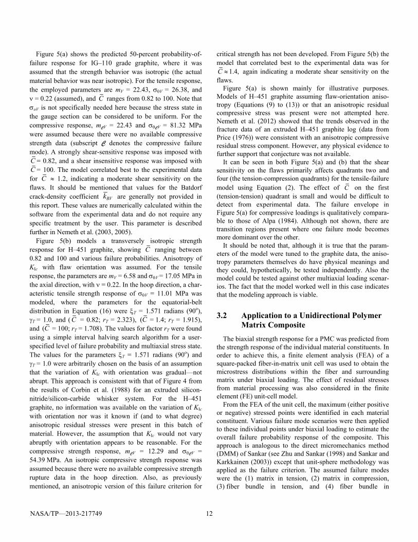
3.2.2 Model M1: Flaw/Failure Plane Anisotropy In model M1 (interactive and noninteractive versions), frac-

ture is assumed to be confined to specific failure planes or

“action planes” in a manner similar to Puck’s theory. The interactive version uses stress results from the unit-cell FEA, and the noninteractive version uses only the applied composite (macroscopic) stresses. The M1 model variation uses the flaw-orientation anisotropy model described by Equations (9) to (13).

For the fiber failure mode in tension, the failure is assumed to result from microscopic flaws in the fiber volume that are highly aligned perpendicular to the fiber axis or are confined to global failure planes as mentioned in Section 2.3.1. Fiber failure, therefore, only becomes a function of the tensile stress applied along the fiber axis (assuming in this case that the shear traction on these planes is negligible). This corresponds to the polar-cap distribution as shown in Figure 2 (and Eq. (12)), whereby the fiber axis is parallel to the x material coordinate system stress axis. Effective stress is calculated for this failure mode, using Equation (2). For the fiber compres-sion failure mode, only the compressive normal stress compo-nent is used to evaluate failure in the manner previously described in Section 2.3.1. Here L is assumed to be 1.0 with a uniform distribution (equal likelihood) of orientation over that increment (L = 0.0) for the polar-cap distribution.

For the matrix failure modes of model M1, the flaws or failure planes are assumed to be highly confined in an equatorial-belt distribution as depicted schematically in Figure 8 (also Fig. 2) and described by Equation (13), whereby T is 1.0 with a uniform distribution (equal likelihood) of orientation over that increment (T = 0.0). The tightly confined equatorial belt distribution is meant to approximate an interfacial flaw population (or global failure planes) between the fiber and the matrix. For the tensile-failure mode, Equation (2) is used to describe the effective stress, whereas for the compressive-failure mode, Equation (19) is used.

Table IV lists the parameters for these various failure modes for the interactive M1 model without the effect of the residual thermal stresses from processing, and Table V lists the param-eters that include the effects of residual stresses from thermal processing. The characteristic strength V is set to the value where the probability of failure is 50 percent for the overall composite loads indicated in Table II. The values of the charac-teristic strength are a function of the stresses at the sampled points in the fiber and matrix for the unit-cell micromechanics FE model. These values reflect the levels of stress concentration in the fiber and matrix predicted from the FE model.

A noninteractive version of the M1 model was also devel-oped. The noninteractive model has the same unit-sphere modeling assumptions as the interactive version of M1 except that it uses the global applied composite stresses—not the unit-cell microstresses of the fiber and matrix. The approach of using global applied composite stresses is similar to other polynomial failure criteria such as Tsai-Wu and Tsai-Hill. The noninteractive model did not consider the effect of thermal residual stresses. The parameters for the noninteractive M1 model are given in Table VI. The values for V were deter-mined such that the composite strength values listed in Table II correspond to a 50-percent probability of failure.

NASA/TP—2013-217749 18

Figure 8.—Model M1—matrix fracture planes are confined to be randomly oriented normal to the fiber axis; x, y, and z, orthogonal stresses.

TABLE IV.—INTERACTIVE MODEL M1 UNIT-SPHERE PARAMETERS WITHOUT RESIDUAL THERMAL STRESSES FROM PROCESSING

[One-half angle of anisotropy distribution, , 1.0; exponent of sine or cosine function, , 0.0.] Failure mode Model and modea Weibull

modulus, mV

Characteristic strength, V, MPa

Shetty shear-sensitivity

constant, C

Fiber: tensile L flaw anisotropic 10.0 2147 1.4 Fiber: compressive L flaw anisotropic 10.0 1346 NAb Matrix: transverse tensile T flaw anisotropic 10.0 79.19 1.4 Matrix: transverse compressive T flaw anisotropic 10.0 181.8 NAb aL, longitudinal; T, transverse. bNA, not applicable.

TABLE V.—INTERACTIVE MODEL M1 UNIT-SPHERE PARAMETERS WITH RESIDUAL THERMAL STRESSES FROM PROCESSING

[One-half angle of anisotropy distribution, , 1.0; exponent of sine or cosine function, , 0.0.] Failure mode Model and modea Weibull

modulus, mV

Characteristic strength, V, MPa

Shetty shear-sensitivity

constant, C

Fiber: tensile L flaw anisotropic 10.0 2128 1.4 Fiber: compressive L flaw anisotropic 10.0 1358 NAb Matrix: transverse tensile T flaw anisotropic 10.0 57.15 1.4 Matrix: transverse compressive T flaw anisotropic 10.0 232.9 NAb aL, longitudinal; T, transverse. bNA, not applicable.

NASA/TP—2013-217749 19

TABLE VI.—NONINTERACTIVE MODEL M1 UNIT-SPHERE PARAMETERS [One-half angle of anisotropy distribution, , 1.0; exponent of sine or cosine function, , 0.0.]

Failure mode Model and modea Weibull modulus,

mV

Characteristic strength, V, MPa

Shetty shear-sensitivity

constant, C

Fiber: tensile

L flaw anisotropic 10.0 1328 1.4 L flaw anisotropic 20.0 1304 1.4

Fiber: compressive

L flaw anisotropic 10.0 829.9 NAb L flaw anisotropic 20.0 814.8 NAb

Matrix: transverse tensile

T flaw anisotropic 10.0 41.49 1.4 T flaw anisotropic 20.0 40.74 1.4

Matrix: transverse compressive T flaw anisotropic 10.0 150.4 NAb T flaw anisotropic 20.0 149.7 NAb

aL, longitudinal; T, transverse. bNA, not applicable.

Figure 9.—Comparison of failure models for 50-percent probability of failure for the combined

failure modes of the M1 (anisotropic flaw plane/global failure plane) model relative to the macroscopic applied stresses. Also shown is a noninteractive model and Tsai-Wu and Tsai-Hill models for comparison. The failure envelopes for the two interactive models for the Weibull modulus for the volume-flaw failure mode, mV = 10, are shown with and without considering the predicted residual stresses resulting from processing. For the matrix tensile failure mode, Shetty shear-sensitivity constant C = 1.4.

3.2.2.1 Model M1 Results

Biaxial failure envelopes for a predicted overall 50-percent probability of failure for the combined failure modes (via Eq. (18) of Section 2.3) were generated with the unit-sphere algorithm for the M1 models for the four failure modes. These results are shown in Figure 9 relative to the macroscopic (composite) applied stresses. The Shetty shear-sensitivity parameter C = 1.4 for the tensile-failure modes was used. This parameter only has a limited effect, which will be shown later for models M2 and M3. Results from the Tsai-Wu and Tsai-Hill failure criteria are also shown in Figure 9 for comparison. The Tsai-Wu and Tsai-Hill criteria, as used here, are based on global

applied stresses and, therefore, do not consider the effect of thermal residual stresses. Figure 9 also shows the overall failure envelopes considering all failure modes for the noninteractive M1 model for mV = 10 and 20 (where all failure modes have the same Weibull modulus value for each failure envelope) compar-ing the effect of mV on the shape of the failure envelope.

Figure 9 shows the adjusted experimental data (Al-Khalil et al. (1996)) used in the WWFE exercise. What is immedi-ately apparent is that the Tsai-Wu criterion fits to the (limited amount of) experimental data quite well. Tsai-Hill also fits the data well in the fourth quadrant (longitudinal tension and transverse compression) but is conservative in the first quadrant (axial tension and transverse tension). The M1

NASA/TP—2013-217749 20

models fit less well to the data in the fourth quadrant. The M1 models are significantly different from Tsai-Wu and Tsai-Hill in all quadrants. In fact the noninteractive M1 model is nearly identical to the maximum principal stress failure criterion (see Fig. 3 in Zhu and Sankar (1998), for example) except that the corners of the envelope are slightly rounded because of the effect of Equation (18) for separate failure modes and the value of Weibull modulus mV that was used. The effect of mV is shown for the noninteractive model where the higher value of mV = 20 appears to sharpen the “corners” of the failure envelope in comparison to the envelope for mV = 10. The noninteractive M1 results are also qualitatively similar in appearance to those presented in Puck and Schurmann (2004).

The interactive M1 model does show some differences from the noninteractive model in Figure 9. This difference is most pronounced in the fourth quadrant, and it illustrates the effect that the microstresses have on the predicted failure probability. For the most part, the envelopes with and without the account-ing of thermal residual stresses from processing were quite similar, except in the first quadrant, where the results without the residual thermal stresses were noticeably unconservative. The reason for the overall similarity was that the failure envel-opes were normalized to the experimental test data of Table II (which already include any effect from thermal residual stresses). Interestingly, the failure envelope without thermal load bears a qualitative resemblance to results from Zhu and Sankar (1998) for the particular DMM case (Von-Mises failure criterion for the fiber and matrix and no interfacial failure criterion) that was illustrated in Figure 3 of that paper. Some of the reasons that the interactive M1 failure envelopes took the shapes that they did are examined next. This line of inquiry was not pursued in the Zhu and Sankar (1998) paper.

3.2.2.2 For M1: Tracking the Response of Individual Sampling Points and Failure Modes

Figure 10 shows the interactive M1 model for the individual sample points at 50-percent probability of failure relative to the applied macroscopic composite stresses for both the case with and the case without the thermal residual stresses. The failure contour lines closest to the origin dominate the failure response and create the enclosed region about the origin that results in the overall failure envelope shown in Figure 9. What is immediately apparent in Figure 10 is that the left-edge sampling point dominates the matrix failure response followed by the left interface sampling point for matrix tensile failure. The matrix top edge and top interface sampling points had little influence.

For the fiber failure modes (tension and compression)—the fiber left edge and fiber top edge—sampling points gave similar results as indicated by the vertical lines in Figure 10. These fiber failure modes indicate little influence from the matrix and transverse loading on fiber failure, as would be expected based on failure mode modeling assumptions and the small relative influence that the matrix has on the fibers. For the matrix, the influence of changing stress state is seen as a

deviation from a horizontal line. For example, in the fourth quadrant there is an increasing compressive stress for y for the left edge and interface sampling points with increasing longitudinal (axial) load as shown in Figures 7(c) and (d), which influences the matrix compressive-failure mode by increasing the probability of failure with the increasing longitudinal load. The decreasing compressive stress for z with increasing longitudinal load shown in Figures 7(e) and (f) has little influence because the magnitude of the compressive stress z is significantly smaller than that of y regardless of the level of applied longitudinal stress (within the range of interest). The x stress had no effect on the matrix probability of failure (see Figs. 7(a) and (b)) because the M1 model assumed that the flaw planes or global failure planes were essentially parallel to that direction of stress. Finally, the differences between the individual-sampled-point probability-of-failure contour lines without thermal residual stresses (Fig. 10(a)) and with thermal residual stresses (Fig. 10(b)) are not that significant, except perhaps in the first quadrant. Figure 11 shows the combined effect of all the sample points on the individual failure modes for a 50-percent failure probability for both cases with and without the residual thermal stresses present. Figure 11 provides a clearer picture of the relative contribution of the individual failure modes.

3.2.3 Model M2: Isotropic Matrix Material In model M2, the matrix was assumed to be an isotropic

strength response material, and the compressive-fiber failure mode was not used. This model only used the unit-cell microstresses. Because the strength response of the matrix was assumed to be isotropic, the M2 model also predicts the matrix strength response for applied uniaxial tensile and compressive loading in the longitudinal (fiber) direction. This differs from M1, where flaw planes or failure planes were oriented parallel to the fiber direction, and hence, matrix failure could not occur regardless of the magnitude of load (infinite matrix strength in this direction, meaning that the fiber was always assumed to fail before the matrix).

M2 used the same tensile-stress fiber-failure-mode model as M1. The matrix tensile-failure mode and the matrix compressive-failure mode both used an isotropic strength response model of the unit sphere (Section 2.1). The effective stress equations (Eqs. (2) and (19)) were used for the tensile and compressive matrix failure modes, respectively. Table VII lists the parameters for the failure modes without the effect of the residual thermal stresses from processing, and Table VIII lists the parameters that include the effects of residual stresses from thermal processing. Only results for the Shetty shear-sensitive parameter C = 1.4 for the tensile-failure modes are given. As described in Section 3.2.2 for model M1, the characteristic strength V was set to that value at which the probability of failure was 50 percent when a uniaxial load was applied at a specified magnitude and direction, as listed in Table II.

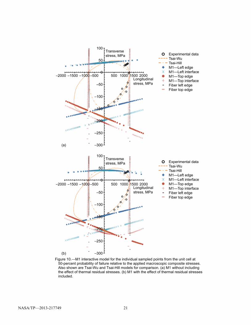
NASA/TP—2013-217749 21

Figure 10.—M1 interactive model for the individual sampled points from the unit cell at

50-percent probability of failure relative to the applied macroscopic composite stresses. Also shown are Tsai-Wu and Tsai-Hill models for comparison. (a) M1 without including the effect of thermal residual stresses. (b) M1 with the effect of thermal residual stresses included.

NASA/TP—2013-217749 22

Figure 11.—M1 interactive model for the individual failure modes from the unit cell at

50-percent probability of failure relative to the applied macroscopic composite stresses. Also shown are Tsai-Wu and Tsai-Hill models for comparison. (a) M1 without including the effect of thermal residual stresses. (b) M1 with the effect of thermal residual stresses included.

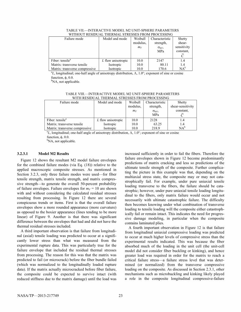
NASA/TP—2013-217749 23

TABLE VII.—INTERACTIVE MODEL M2 UNIT-SPHERE PARAMETERS WITHOUT RESIDUAL THERMAL STRESSES FROM PROCESSING

Failure mode Model and mode Weibull modulus,

mV

Characteristic strength, V, MPa

Shetty shear-

sensitivity constant,

C Fiber: tensilea L flaw anisotropic 10.0 2147 1.4 Matrix: transverse tensile Isotropic 10.0 80.11 1.4 Matrix: transverse compressive Isotropic 10.0 170.6 NAb aL, longitudinal; one-half angle of anisotropy distribution, , 1.0; exponent of sine or cosine function, , 0.0. bNA, not applicable.

TABLE VIII.—INTERACTIVE MODEL M2 UNIT-SPHERE PARAMETERS WITH RESIDUAL THERMAL STRESSES FROM PROCESSING

Failure mode Model and mode Weibull modulus,

mV

Characteristic strength, V, MPa

Shetty shear-sensitivity

constant, C

Fiber: tensilea L flaw anisotropic 10.0 2128 1.4 Matrix: transverse tensile Isotropic 10.0 63.25 1.4 Matrix: transverse compressive Isotropic 10.0 218.9 NAb aL, longitudinal; one-half angle of anisotropy distribution, , 1.0; exponent of sine or cosine function, , 0.0. bNA, not applicable.

3.2.3.1 Model M2 Results Figure 12 shows the resultant M2 model failure envelopes

for the combined failure modes (via Eq. (18)) relative to the applied macroscopic composite stresses. As mentioned in Section 3.2.3, only three failure modes were used—for fiber tensile strength, matrix tensile strength, and matrix compres-sive strength—to generate the overall 50-percent probability of failure envelopes. Failure envelopes for mV = 10 are shown with and without considering the calculated residual stresses resulting from processing. In Figure 12 there are several conspicuous trends or items. First is that the overall failure envelopes show a more rounded appearance (more curvature) as opposed to the boxier appearance (lines tending to be more linear) of Figure 9. Another is that there was significant difference between the envelopes that had and did not have the thermal residual stresses included.

A third important observation is that failure from longitudi-nal (axial) tensile loading was predicted to occur at a signifi-cantly lower stress than what was measured from the experimental rupture data. This was particularly true for the failure envelope that included the residual thermal stresses from processing. The reason for this was that the matrix was predicted to fail (or microcrack) before the fiber bundle failed (which was normalized to the longitudinally loaded rupture data). If the matrix actually microcracked before fiber failure, the composite could be expected to survive intact (with reduced stiffness due to the matrix damage) until the load was

increased sufficiently in order to fail the fibers. Therefore the failure envelopes shown in Figure 12 become predominantly predictions of matrix cracking and less so predictions of the ultimate tensile strength of the composite. Further complica-ting the picture in this example was that, depending on the multiaxial stress state, the composite may or may not cata-strophically fail. For example, under pure uniaxial tensile loading transverse to the fibers, the failure should be cata-strophic; however, under pure uniaxial tensile loading longitu-dinal to the fibers, only matrix failure would occur and not necessarily with ultimate catastrophic failure. The difficulty then becomes knowing under what combination of transverse loading to tensile loading will the composite either catastroph-ically fail or remain intact. This indicates the need for progres-sive damage modeling, in particular when the composite contains laminated plies.

A fourth important observation in Figure 12 is that failure from longitudinal uniaxial compressive loading was predicted to occur at much higher levels of compressive stress than the experimental results indicated. This was because the fiber absorbed much of the loading in the unit cell (the unit-cell model did not consider fiber buckling or kinking), and hence greater load was required in order for the matrix to reach a critical failure stress—a failure stress level that was deter-mined (or normalized) from the transverse compressive loading on the composite. As discussed in Section 2.3.1, other mechanisms such as microbuckling and kinking likely played a role in the composite longitudinal compressive-failure

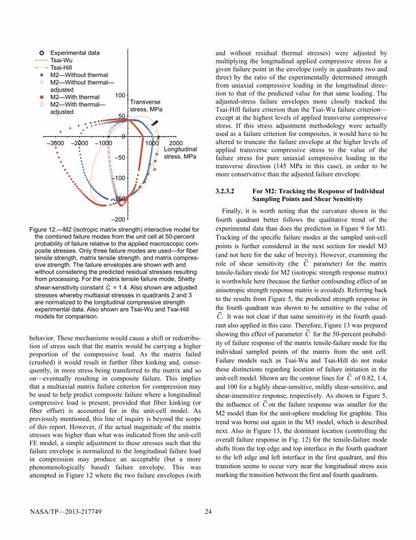
NASA/TP—2013-217749 24

Figure 12.—M2 (isotropic matrix strength) interactive model for

the combined failure modes from the unit cell at 50-percent probability of failure relative to the applied macroscopic com-posite stresses. Only three failure modes are used—for fiber tensile strength, matrix tensile strength, and matrix compres-sive strength. The failure envelopes are shown with and without considering the predicted residual stresses resulting from processing. For the matrix tensile failure mode, Shetty shear-sensitivity constant C = 1.4. Also shown are adjusted stresses whereby multiaxial stresses in quadrants 2 and 3 are normalized to the longitudinal compressive strength experimental data. Also shown are Tsai-Wu and Tsai-Hill models for comparison.

behavior. These mechanisms would cause a shift or redistribu-tion of stress such that the matrix would be carrying a higher proportion of the compressive load. As the matrix failed (crushed) it would result in further fiber kinking and, conse-quently, in more stress being transferred to the matrix and so on—eventually resulting in composite failure. This implies that a multiaxial matrix failure criterion for compression may be used to help predict composite failure where a longitudinal compressive load is present, provided that fiber kinking (or fiber offset) is accounted for in the unit-cell model. As previously mentioned, this line of inquiry is beyond the scope of this report. However, if the actual magnitude of the matrix stresses was higher than what was indicated from the unit-cell FE model, a simple adjustment to these stresses such that the failure envelope is normalized to the longitudinal failure load in compression may produce an acceptable (but a more phenomenologically based) failure envelope. This was attempted in Figure 12 where the two failure envelopes (with

and without residual thermal stresses) were adjusted by multiplying the longitudinal applied compressive stress for a given failure point in the envelope (only in quadrants two and three) by the ratio of the experimentally determined strength from uniaxial compressive loading in the longitudinal direc-tion to that of the predicted value for that same loading. The adjusted-stress failure envelopes more closely tracked the Tsai-Hill failure criterion than the Tsai-Wu failure criterion—except at the highest levels of applied transverse compressive stress. If this stress adjustment methodology were actually used as a failure criterion for composites, it would have to be altered to truncate the failure envelope at the higher levels of applied transverse compressive stress to the value of the failure stress for pure uniaxial compressive loading in the transverse direction (145 MPa in this case), in order to be more conservative than the adjusted failure envelope.

3.2.3.2 For M2: Tracking the Response of Individual Sampling Points and Shear Sensitivity

Finally, it is worth noting that the curvature shown in the fourth quadrant better follows the qualitative trend of the experimental data than does the prediction in Figure 9 for M1. Tracking of the specific failure modes at the sampled unit-cell points is further considered in the next section for model M3 (and not here for the sake of brevity). However, examining the role of shear sensitivity (the C parameter) for the matrix tensile-failure mode for M2 (isotropic strength response matrix) is worthwhile here (because the further confounding effect of an anisotropic strength response matrix is avoided). Referring back to the results from Figure 5, the predicted strength response in the fourth quadrant was shown to be sensitive to the value of

.C It was not clear if that same sensitivity in the fourth quad-rant also applied in this case. Therefore, Figure 13 was prepared showing this effect of parameter C for the 50-percent probabil-ity of failure response of the matrix tensile-failure mode for the individual sampled points of the matrix from the unit cell. Failure models such as Tsai-Wu and Tsai-Hill do not make these distinctions regarding location of failure initiation in the unit-cell model. Shown are the contour lines for C of 0.82, 1.4, and 100 for a highly shear-sensitive, mildly shear-sensitive, and shear-insensitive response, respectively. As shown in Figure 5, the influence of C on the failure response was smaller for the M2 model than for the unit-sphere modeling for graphite. This trend was borne out again in the M3 model, which is described next. Also in Figure 13, the dominant location (controlling the overall failure response in Fig. 12) for the tensile-failure mode shifts from the top edge and top interface in the fourth quadrant to the left edge and left interface in the first quadrant, and this transition seems to occur very near the longitudinal stress axis marking the transition between the first and fourth quadrants.

NASA/TP—2013-217749 25

Figure 13.—M2 model of the matrix tensile failure mode versus the applied macroscopic com-

posite stress showing the effect of the Shetty shear-sensitivity constant, C , on the 50-percent probability of failure response of the individual sampled points of the matrix in the unit cell. Shown are the contour lines for C of 0.82, 1.4, and 100, for a highly shear-sensitive, a mildly shear-sensitive, and shear-insensitive response, respectively. Only the loading case without considering residual thermal stresses from processing is shown. Also shown are Tsai-Wu and Tsai-Hill models for comparison.

3.2.4 Model M3: Anisotropic Matrix Material

In this model variation, designated as M3, the matrix was assumed to be mildly anisotropic in strength response. This was done specifically so that the matrix did not fail (or microcrack) prior to fiber bundle failure under longitudinal tensile loading. As with M2, this model only used the unit-cell microstresses. Two model variants are described: M3a and M3b. M3a used the tensile fiber failure mode described in M1 but excluded the compressive fiber failure mode (similar to what was done with M2). M3b used the same tensile- and compressive-stress fiber failure modes as M1. In M3a and M3b, the matrix tensile-failure mode was assumed to have a mildly anisotropic strength response; however, the matrix compressive-failure mode used the same isotropic strength response model of M2.

Table IX lists the parameters for the failure modes that do not include the effect of the residual thermal stresses from

processing, and Table X lists the parameters for the failure modes that include the effects of residual stresses from thermal processing. Only results with the Shetty shear-sensitive parameter C = 1.4 for the tensile-failure mode are listed. As previously described with M1, the characteristic strength V was set to a value whereby the probability of failure was 50 percent when a uniaxial load was applied at the magnitude and direction specified in Table II. For the matrix tensile-failure mode, the parameters were set for an applied tensile load that was parallel to the fiber direction at an arbitrarily set value of 1500 MPa (a value not listed in Table II), which was sufficiently stronger, for the purpose of this example, than the fiber bundle strength for the applied macroscopic load of 1280 MPa. The degree of strength anisotropy was set so that for an applied uniaxial tensile load transverse to the fiber, the strength was 40 MPa (see Table II) at a probability of failure of 50 percent.

NASA/TP—2013-217749 26

TABLE IX.—INTERACTIVE MODEL M3a AND M3b UNIT-SPHERE PARAMETERS WITHOUT RESIDUAL THERMAL STRESSES FROM PROCESSING

Failure mode Model and mode Weibull modulus,

mV

Characteristic strength, V, MPa

Shetty shear-sensitivity

constant, C

Fiber: tensilea,b L flaw anisotropic 10.0 2147 1.4 Fiber: compressivea,b,c L flaw anisotropic 10.0 1346 -- Matrix: transverse tensiled T critical strength anisotropic 10.0 111.8 1.4 Matrix: transverse compressivea Isotropic 10.0 170.6 -- aThe constants , , and r are not used. bL, longitudinal; one-half angle of anisotropy distribution, , 1.0; exponent of sine or cosine function, , 0.0. cFailure mode used with model M3b. dSet for 1500-MPa longitudinal strength at 50-percent probability of failure; one-half angle of anisotropic distribution for critical mode I stress intensity factor, , 10; exponent of sine or cosine function, , 1.0; constant, r, 1.776.

TABLE X.—INTERACTIVE MODEL M3A AND M3B UNIT-SPHERE PARAMETERS WITH RESIDUAL THERMAL STRESSES FROM PROCESSING

Failure mode Model and mode Weibull modulus,

mV

Characteristic strength, V, MPa

Shetty shear-sensitivity

constant, C

Fiber: tensilea,b L flaw anisotropic 10.0 2128 1.4 Fiber: compressivea,b,c L flaw anisotropic 10.0 1358 -- Matrix: transverse tensiled T critical strength anisotropic 10.0 127.7 1.4 Matrix: transverse compressivea Isotropic 10.0 218.9 -- aThe constants , , and r are not used. bL, longitudinal; one-half angle of anisotropy distribution, , 1.0; exponent of sine or cosine function, , 0.0. cFailure mode used with model M3b. dSet for 1500-MPa longitudinal strength at 50-percent probability of failure; one-half angle of anisotropic distribution for critical mode I stress intensity factor, , 10; exponent of sine or cosine function, , 1.0; constant, r, 2.959.

The anisotropic strength response was achieved by using the

critical-strength and stress-intensity-factor anisotropy model described by Equations (16) and (17) for an equatorial-belt distribution (see Fig. 3) of angular width T = 0.1745 radians (10) and shape exponent T = 1.0. The values for parameters T and T were chosen arbitrarily, but they were set so that a rather abrupt variation of Ic with orientation occurred. This was meant to physically simulate a weaker interface between the fiber and the matrix or to be indicative of flaws having a lower average strength (or larger average length) normal to (or nearly normal to) the fiber axis orientation in comparison to other orientations. A simple interval halving search algorithm was used to find the values for rT for a user-specified level of failure probability and multiaxial stress state. Tables IX and X list these values without considering residual thermal stresses and considering residual thermal stresses, respectively.

The amount of strength anisotropy in the matrix is seen by comparing the characteristic strength V between models M3 and M2. For example, for the characteristic strength without

residual stresses, this difference was 111.8 MPa for the anisotropic strength matrix versus 80.11 MPa for the isotropic matrix (in Tables IX and VII, respectively) for a 1.396 strength ratio. For the value of V that included the effects of residual thermal stresses, this difference was 127.7 MPa for the anisotropic strength matrix versus 63.25 MPa for the isotropic matrix (in Tables X and VIII, respectively) for a higher strength ratio of 2.019. The reason for the increased stress ratio can be seen in Figure 12, where a larger amount of adjustment is required for the case with the thermal residual stresses than for the case without the thermal residual stresses in order to normalize the longitudinal tensile strength response to the 1500 MPa value.

3.2.4.1 Model M3 Results Figure 14 shows the resultant failure envelopes for models

M3a and M3b for the combined failure modes (via Eq. (18)) considering and not considering the residual stresses from thermal processing. The M3a model is also shown with and

NASA/TP—2013-217749 27

Figure 14.—M3a and M3b (anisotropic tensile failure mode for matrix) interactive models for the

combined failure modes from the unit cell at 50-percent probability of failure relative to the applied macroscopic composite stresses. Also shown are adjusted stresses whereby multiaxial stresses in quadrants 2 and 3 are normalized to the longitudinal compressive strength experimental data. Model M3b is the same as M3a with the addition of the simple longitudinal compressive failure criterion. All failure envelopes are shown with and without considering the predicted residual stresses that resulted from processing. For the matrix tensile failure mode, Shetty shear-sensitivity constant C = 1.4 was assumed. Also shown are Tsai-Wu and Tsai-Hill models for comparison.

without the adjusted stresses (as per M2). From the figure it is observed that allowing the strength response of the matrix in tension to be anisotropic brought the failure envelopes in better alignment with the experimental data in the fourth quadrant (both with and without including the effects of residual thermal stresses) and closer to (or between) the results of the Tsai-Wu and Tsai-Hill failure criteria. The M3 and M2 models illustrate the caution that must be exercised when applying Equation (18): it is important to know what the predominant failure modes are and whether or not they imply ultimate composite failure.

In quadrant one of Figure 14, the results from the M3 model that included and did not include residual stresses were in closer agreement than were the results from the M1 model in Figure 9, although the M3 model results were also slightly more conservative in comparison to the experimental data shown in that quadrant. The predicted envelopes fell between the Tsai-Wu and Tsai-Hill failure envelopes in that quadrant.

There are also some noteworthy features in quadrants two and three. With the M3a model (with and without the effect of residual stresses), the failure envelopes for the unadjusted stresses do show some difference in shape relative to the failure envelope of the M2 model in Figure 12. This was particularly surprising in quadrant three because both the M2 and M3a models used the same isotropic strength response model for the matrix in compression. This discrepancy is explored further when the individual failure modes are examined. The difference in shape was also transferred to the

adjusted stresses, where the predicted results were somewhat more nonconservative in comparison to the Tsai-Hill criterion than were the results in Figure 12. Nevertheless, the trend remained that the adjusted stresses tracked much closer to the Tsai-Hill criterion than to the Tsai-Wu criterion. Quadrants two and three of Figure 14 also show the effect of the fiber failure mode in compression for model M3b. Although employing this failure mode was a somewhat trivial exercise, it was useful to compare the predictions of this failure mode to the predictions with the adjusted stresses. Overall, Figure 14 showed that the M3a model with the stresses adjusted in quadrants two and three followed the experimental data reasonably well and also that the failure envelopes (with and without considering residual thermal stresses) tracked rela-tively close to the Tsai-Hill failure criterion.

3.2.4.2 For M3: Tracking the Response of Individual Sampling Points and Failure Modes

Figure 15 shows the matrix tensile and compressive-failure modes for the individual sampled points in the unit cell for the M3a model without consideration of the effect of residual thermal stresses from processing. This figure reveals that the dominant failure modes were relative to the stress quadrant as well as the sampling points that were the source for this behavior. To see the contribution of the fiber failure modes, refer back to Figures 10 and 11. Some interesting trends are revealed in Figure 15. For example, the top edge sampling-point is shown to contribute significantly to matrix failure in

NASA/TP—2013-217749 28

Figure 15.—M3a model of individual points for 50-percent probability of failure for the matrix

compressive (C) and matrix tensile (T) failure modes without consideration of the effect of the residual stresses from thermal processing. For the matrix tensile failure mode, Shetty shear-sensitivity constant C = 1.4 was assumed. Also shown are Tsai-Wu and Tsai-Hill models for comparison.

the third quadrant (also compare this with Fig. 10) in both the tensile and compressive-failure modes. Also, in the third quadrant for the most extreme compressive loading case (the combination of the highest longitudinal and transverse compressive stresses acting simultaneously), a tensile-failure mode is indicated.

In the fourth quadrant of Figure 14, the failure envelope showed a curved path (or rounded corner). Figure 15 indicates that a major factor in this behavior was the compressive-failure mode at the left-edge sampling point. This contrasts with Figure 5 for graphite where the tensile-failure mode played a more prominent role in this (fourth) quadrant as evidenced by the role that the shear-sensitivity parameter C played in the resultant shape of the failure envelope. Another interesting observation in the fourth quadrant was that the tensile-failure mode at the top edge and top interface points played a significant role in matrix failure at the higher levels of applied longitudinal tensile stress. In the M2 model shown in Figure 12, these failure contour lines shifted to the left (became weaker) and resulted in the matrix being predicted to microcrack before fiber bundle failure would likely occur. Also of note in Figure 15 was that the location for the tensile-failure mode shifts from the top edge and top interface in the fourth quadrant to the left edge and left interface in the first quadrant and that this transition seems to occur very near the portion of the longitudinal stress axis that marks the transition between the first and fourth quadrants. This was also indicated to occur in the M2 model in Figure 13. Also, in the first quadrant of Figure 15 it can be seen that the prediction of

matrix failure correlated well with the experimental data. The greater conservatism seen in the failure envelope in Figure 14 was, therefore, due to the added effect of the fiber tensile-failure mode on the overall failure probability via Equation (18). The experimental data in the first quadrant were actually an adjustment made by Al-Khalil et al. (1996) that added a transverse tensile-stress component to what was originally intended as pure longitudinal tensile loading. A fiber failure mode was indicated for these data. However, it is also interesting to note that Al-Khalil et al. (1996) initially had difficulty suppressing catastrophic matrix failure transverse to the fiber under longitudinal tensile loading—perhaps illustrat-ing some sensitivity to the transverse loading component.

Figure 16 shows the effect of parameter C for the 50-percent probability-of-failure response of the matrix tensile-failure mode for the individual sampled points of the matrix from the unit cell. The individual points are shown (as opposed to the overall failure probability) so that the rela-tive contribution and sensitivity to C of each point location on the overall failure probability can also be seen. Shown are the contour lines for C of 0.82, 1.4, and 100 for a highly shear-sensitive, a mildly shear-sensitive, and a shear-insensitive response, respectively. Figure 16 shows that the influence of C on the failure response was small for the M3 models in comparison to the unit-sphere modeling for graphite shown in Figure 5. This confirmed that adding strength anisotropy to the M3 model did not appreciably affect the behavior of C in comparison to the results from M2 shown in Figure 13 for the isotropic strength response matrix.

NASA/TP—2013-217749 29

Figure 16.—M3a model of matrix tensile failure mode showing the effect of the shear sensitivity

parameter C (without thermal residual stresses). Also shown are Tsai-Wu and Tsai-Hill models for comparison.

Overall, the M3 models provided better correlation to the experimental data than did the M1 and M2 unit-sphere models (depending on when matrix microcracking initiated). Better correlation to the experimental data in the fourth quadrant could have been achieved if the strength anisotropy in the matrix had been reduced by making it weaker in the fiber direction. However, doing so would have implied that matrix failure would become more predominant over the fiber failure mode at the highest levels of applied longitudinal stress, and this was not pursued.

4.0 Summary and Conclusions This report introduced the unit-sphere methodology to the

problem of multiaxial strength response for brittle or quasi-brittle anisotropic and composite materials. This required the development of modeling extensions that allowed for (1) flaw-orientation anisotropy, whereby a preexisting microcrack has a higher likelihood of being oriented in one direction over another direction; and (2) critical strength or fracture tough-ness anisotropy, whereby the level of critical strength Ic or fracture toughness KIc for mode I crack propagation changes with regard to the orientation of the microstructure. This was done for transversely isotropic strength response materials for the tensile mode of failure. In addition, a simple shear-stress-based unit-sphere failure criterion was introduced to account for the compressive mode of failure for isotropic-strength-response materials. A central principle to this model was that various failure modes controlled the material strength response

and that these modes are stochastic and described by a Weibull distribution. The probability of material survival (the inverse of probability of failure) was the product of the probabilities of survival for the various failure modes. This assumed that weakest-link behavior was operative with no interactivity between failure modes.

The unit-sphere model for anisotropic strength response was applied to nuclear-grade IG–110 and H–451 graphite and to a unidirectional-fiber-reinforced polymer-matrix composite under biaxial loading situations (uniaxial loads applied orthogonal to one another). First, this was done to demonstrate the methodology for a macroscopically homogeneous material and, subsequently, for a heterogeneous material system.

For the nuclear-grade graphite, failure envelopes for con-stant levels of probability of failure for biaxial loading were generated for an isotropic strength response material (the IG–110 grade) and a mildly anisotropic strength response material (the H–451 grade). The experimental data for pure uniaxial loading were used to normalize or calibrate the models. The Shetty shear-sensitive mixed-mode fracture criterion with an assumed penny-shaped crack modeled the flaws in the materials for the tensile-failure mode, and the sim-ple shear-based failure criterion was used to predict the response for the compressive-failure mode. Good correlation was achieved for the H–451 rupture data, which was available only for the first and fourth biaxial-loading quadrants (the isotropic strength response for the near-isotropic IG–110 grade material was shown mainly for comparison purposes). Failure envelopes that assumed highly shear-sensitive (to mode II)

NASA/TP—2013-217749 30

and shear-insensitive flaws were also shown. The model indicated that the level of shear sensitivity significantly affected the predicted strength response in the fourth loading quadrant (for applied tensile and compressive stresses) and that a mildly shear-sensitive flaw response correlated best to the experimental data.

For the unidirectional composite problem, the test case from the WWFE for the unidirectional lamina under combined longitudinal and transverse loading was chosen. An FE model of a continuous-fiber-reinforced composite unit cell with square packing was examined. The thermal residual stresses that develop from processing (during cooldown) were also accounted for in the linear-elastic stress analysis. The stress analysis revealed that four locations (two of the locations were coincident with the fiber matrix interface) contained the highest magnitude stresses. These four locations were subse-quently used in the context of a maximum-stressed-point failure criterion to predict the probability of failure of the composite. Failure envelope predictions (at 50-percent probability of failure) from the unit-sphere model were compared with the experimental results of the WWFE test case as well as to the well-known Tsai-Wu and Tsai-Hill failure criteria.

Four failure modes were assumed to be active for the composite material: (1) fiber failure in tension, (2) fiber failure in compression, (3) matrix failure in tension, and (4) matrix failure in compression. Three variations of the anisotropic unit-sphere model were examined—designated as M1 (flaw and failure plane anisotropy), M2 (isotropic matrix strength), and M3 (anisotropic matrix strength). The major assumption behind the M1 model was that the flaw planes in the matrix were either oriented parallel to the fiber axis or that strength was controlled by global failure (action) planes that ran parallel to the fiber axis. A noninteractive version of M1 that used only applied global macroscopic stresses also was investigated. The resulting failure envelopes (with thermal residual stresses and without thermal residual stresses) did not agree with the experimental data well in the fourth stress quadrant. It was shown that a transverse stress component in the matrix that became more compressive as longitudinal load increased affected the compressive-failure mode and was responsible for the shape of the failure envelope in the fourth quadrant. The noninteractive M1 version corresponded closely to a stochastic version of the maximum principal-stress failure criterion.

Conversely, the M2 model assumed an isotropic strength matrix, and the compressive fiber failure mode was not considered in the overall failure probability calculation. The resultant failure envelopes took a distinctly more rounded

shape than the results from M1 because of the added contribu-tion of the longitudinal stress component in the matrix. Major findings indicated that (1) the matrix was predicted to micro-crack before the fiber bundle failed, (2) matrix compressive strength was much greater than the composite longitudinal compressive strength, and (3) there were significant differ-ences in the predicted strength response when residual thermal stresses were included as opposed to when they were not. The predicted failure envelopes did not correlate well with either the experimental data or the Tsai-Wu or Tsai-Hill failure criteria. Normalizing (pinning) the longitudinal uniaxial compressive response to the experimental data enabled failure envelopes in biaxial stress quadrants two and three to compare more favorably with the Tsai-Hill failure criterion results in these two quadrants.

The M3 model assumed that the matrix had a mildly aniso-tropic strength response for the tensile-failure mode so that matrix microcracking would be predicted to occur at an applied longitudinal tensile stress that was higher than the experimental strength of the fiber bundle. For M3 the overall failure envelopes tracked quite well to the limited amount of experimental data that were available and clearly provided better correlation than the M1 and M2 models.

The development of the anisotropic unit-sphere methodol-ogy was an attempt to provide an improved mechanistic basis to the problem of predicting composite strength under multi-axial loading compared with phenomenological-based poly-nomial formulations such as Tsai-Wu, Tsai-Hill, and Hashin, among others. This model is not as simple and straightforward to use as these other failure criteria; however, the value of this work is in the insights that are provided about stress-state interactions, possible failure modes, and the physical assump-tions behind predicted behaviors.

Planned future work will incorporate unit-sphere methodol-ogy into the NASA Glenn Research Center micromechanics analysis code/generalized method of cells (MAC/GMC) analysis tool. This will involve the full-field stress solution of the unit cell, including stressed-volume size effects. The ever-expanding capabilities of MAC/GMC combined with the time-stepping (and time- and cycle-dependent) transient reliability analysis capabilities of the unit-sphere algorithm conceivably will allow for stochastic-based progressive damage modeling capability that takes into account time- and cycle-dependent material degradation in a computationally efficient manner.

Glenn Research Center National Aeronautics and Space Administration Cleveland, Ohio, August 1, 2013

NASA/TP—2013-217749 31

Appendix—Symbols A area ac critical crack length or crack radius C Shetty shear-sensitivity coefficient c constant E Young’s modulus of elasticity

I ,cf normalized anisotropy function of KIc or Ic as a function of angles and

H Heaviside step function KI mode I stress-intensity factor KIc critical mode I stress-intensity factor

BVk Batdorf uniaxial stress-state normality constant for the volume-flaw failure mode (also known as the Batdorf nor-malized crack-density coefficient)

m Weibull modulus mCV Weibull modulus for the volume-flaw

failure mode for compressive stress states

mV Weibull modulus for the volume-flaw failure mode

n number of failure modes Pf probability of failure (Pf = 1– Ps) PfV probability of failure of material volume PfV probability of failure of a crack with a

strength between Ic and (Ic + Ic) in V

Ps reliability or probability of survival (Ps = 1 – Pf)

P1V probability of existence of a crack with strength between Ic and (Ic + Ic) in an incremental volume

P2V probability that a crack of critical strength will be oriented in a particular direction such that it will grow and cause failure

(, ) probability that a crack of critical strength Ieqc is oriented in the range between α and (α + dα) and between β and (β + dβ)

rL constant (ratio) or parameter in KIc anisotropy function for polar-cap distribution

rT constant (ratio) or parameter in KIc anisotropy function for equatorial-belt distribution

V volume Ve effective volume x, y, z location in the body of the structure;

Cartesian coordinates Y crack-shape geometry factor ,  orientation angles or angular coordinates,

where the direction normal to the plane of the microcrack is specified by the radial line defined by and in stress space

t thermal expansion coefficient constant or parameter in KIc anisotropy

function representing the exponent of the sine or cosine function

L constant or parameter in KIc anisotropy function representing the longitudinal (polar-cap) distribution

T constant or parameter in KIc anisotropy function representing the transverse (equatorial-belt) distribution

() as a function of angle describing the anisotropy of flaw orientation

(, ) function describing the anisotropy of the flaw orientation where the normal direction to the flaw plane is given by angles and

V(Ieqc) crack-density function for equivalent mode I strength, Ieqc, of a flaw: number of flaws per unit volume with strength equal to or less than Ieqc

angle measured from the longitudinal loading axis

constant or parameter in flaw-orientation anisotropy function repre-senting one-half of the total angular extent of the anisotropy distribution

L constant or parameter in flaw-orientation anisotropy function representing the longitudinal (polar-cap) distribution

T constant or parameter in flaw-orientation anisotropy function or in KIc anisotropy function representing the transverse (equatorial-belt) distribution

Poisson’s ratio constant or parameter in KIc anisotropy

function representing one-half of the total angular extent of the anisotropy distribution

NASA/TP—2013-217749 32

L constant or parameter in KIc anisotropy function representing the longitudinal (polar-cap) distribution

T constant or parameter in KIc anisotropy function representing the transverse (equatorial-belt) distribution

summation function; applied far-field multiaxial stress state

applied uniaxial stress Ic critical mode I strength

z,Iy,Ix,I ,, ccc orthogonal critical strength components

normalized by Ic,max Ieq equivalent, or effective, stress Ieq,max maximum value of Ieq over the unit

sphere from the applied multiaxial stress

Ieqc critical equivalent, or effective, strength Ieqc(x, y, z, , ) critical equivalent, or effective, strength

of a flaw located at coordinates x, y, and z and oriented at angles and

n applied far-field stress component normal to a crack face

oV Weibull scale parameter for the volume-flaw failure mode normalized to unit volume

x, y, z orthogonal stress components expressed relative to a global coordinate system

V Weibull characteristic strength (volume-flaw failure mode)

CV Weibull characteristic compressive strength (volume-flaw failure mode)

shear stress acting on the oblique plane whose normal is determined by angles and , which represents the applied far-field shear stress on a crack face

xy, yz, zx shear stress components expressed relative to a global coordinate system

constant or parameter in flaw-orientation anisotropy function repre-senting the exponent of the sine or cosine function

L constant or parameter in flaw-orientation anisotropy function representing the longitudinal (polar-cap) distribution

T constant or parameter in flaw-orientation anisotropy function representing the transverse (equatorial-belt) distribution

(, Ieqc) area of a solid angle projected onto a unit radius sphere in three-dimensional stress space for which Ieq Ieqc from an applied multiaxial stress state

Superscript – normalized Subscripts C compression

c critical eq equivalent, or effective I mode I i ith value or ith term L longitudinal max maximum T transverse V volume or a volume-based property

(e.g., indicates volume-flaw analysis)

Definitions fast fracture component rupture in the absence

of slow crack growth where strength is strictly controlled by the fracture toughness and the size, distribution, and orientation of inherent flaws

L longitudinal mode I crack-opening mode mode II crack-sliding mode (in-plane

shear) mode III crack-tearing mode (out-of-plane

shear) T transverse transient reliability analysis predicting the probability of

survival of a component while accounting for loads and temper-atures that can vary over time

NASA/TP—2013-217749 33

ReferencesAboudi, J. (1995): Micromechanical Analysis of Thermo-

Inelastic Multiphase Short-Fiber Composites. Compos. Eng., vol. 5, no. 7, pp. 839–850.

Aboudi, Jacob; Pindera, Marek J.; and Arnold, Steven M. (2003): Higher-Order Theory for Periodic Multiphase Materials With Inelastic Phases. Int. J. Plast., vol. 19, pp. 805–847.

Al-Khalil, M.F.S., et al. (1996): The Effects of Radial Stresses on the Strength of Thin-Walled Filament Wound GRP Composite Pressure Cylinders. Int. J. Mech. Sci., vol. 38, no. 1, pp. 97‒120.

Alpa, G. (1984): On a Statistical Approach to Brittle Rupture for Multiaxial States of Stress. Engrg. Fract. Mechan., vol. 19, no. 5, pp. 881–901.

Batdorf, Samuel B. (1973): A Statistical Theory for the Fracture of Transversely Isotropic Brittle Materials of Moderate Anisotropy. Air Force Report SAMSO–TR–73–361, Aerospace Report TR–0074(4450–76)–1, NTIS AD–770982.

Batdorf, S.B. (1978a): Fracture Statistics of Polyaxial Stress States. Fracture Mechanics, Nicholas Perrone, et al., eds., The University Press of Virginia, Charlottesville, VA, pp. 579592.

Batdorf, S.B. (1978b): New Light on Weibull Theory. Nucl. Eng. Des., vol. 47, pp. 267–272.

Batdorf, S.B.; and Crose, J.G. (1974): A Statistical Theory for the Fracture of Brittle Structures Subjected to Nonuni-form Polyaxial Stresses. J. Appl. Mech. Trans. ASME, vol. 41, no. 2, pp. 459464.

Batdorf, S.B.; and Heinisch, H.L., Jr. (1978): Weakest Link Theory Reformulated for Arbitrary Fracture Criterion. J. Am. Ceram. Soc., vol. 61, no. 7, pp. 355358.

Bednarcyk, Brett A.; and Arnold, Steven M. (2002): MAC/GMC 4.0 User’s Manual—Keywords Manual. NASA/TM—2002-212077/VOL 2, http://ntrs.nasa.gov/

Buch, J.D.; Crose, J.G.; and Robinson, E.Y. (1977): Failure Criteria in Graphite Program; Final Report. AFML–TR–77–16. Available from the Air Force Materials Laboratory.

Burchell, Tim; Yahr, Terry; and Battiste, Rick (2007): Modeling the Multiaxial Strength of H‒451 Nuclear Grade Graphite. Carbon, vol. 45, pp. 2570‒2583.

Calard, V.; and Lamon, J. (2002): A Probabilistic-Statistical Approach to the Ultimate Failure of Ceramic-Matrix Compo-sites—Part I: Experimental Investigation of 2D Woven SiC/ SiC Composites. Compos. Sci. Technol., vol. 62, pp. 385‒393.

Corbin, Normand D., et al. (1988): Material Development in the Silicon Nitride-Silicon Carbide Whisker System. Proceedings of the Twenty-sixth Automotive Technology Development Contractors’ Coordination Meeting, Dearborn, MI, Oct. 24–27.

Dassault Systèmes (2010): Abaqus/CAE User’s Manual. https://www.sharcnet.ca/Software/Abaqus610/Documentation/docs/v6.10/books/usi/default.htm Accessed Aug. 1, 2012.

Erdogan, F.; and Sih, G.C. (1963): On the Crack Extension in Plates Under Plane Loading and Transverse Shear. J. Basic Eng., vols. 85, no. 4, pp. 519525.

Evans, A.G. (1978): A General Approach for the Statistical Analysis of Multiaxial Fracture. J. Amer. Ceram. Soc., vol. 61, nos. 7–8, pp. 302–308.

Freudenthal, Alfred M. (1968): Statistical Approach to Brittle Fracture. Fracture: An Advanced Treatise, H. Liebowitz, ed., ch. 6, vol. II, pp. 591–619.

Guillaumat, L.; and Lamon, J. (1996): Probabilistic-Statistical Simulation of the Non-Linear Mechanical Behavior of a Woven SiC/SiC Composite. Compos. Sci. Technol., vol. 56, pp. 803‒808.

Harlow, D.G.; and Phoenix, S.L. (1978): The Chain-of-Bundles Probability Model for the Strength of Fibrous Materials II: A Numerical Study of Convergence. J. Compos. Mat., vol. 12, pp. 314–334.

Hellen, T.K.; and Blackburn, W.S. (1975): The Calculation of Stress Intensity Factors for Combined Tensile and Shear Loading. Int. J. Fract., vol. 11, no. 4, pp. 605617.

Hinton, M.J.; Kaddour, A.S.; and Soden, P.D. (2004): Failure Criteria in Fibre-Reinforced-Polymer Composites: The World-Wide Failure Exercise. Elsevier Ltd., New York, NY.

Hoel, Paul Gerhard; Port, Sidney C.; and Stone, Charles J. (1971): Introduction to Probability Theory. Houghton Mifflin, Boston, MA, pp. 65 and 131.

Ichikawa, Masahiro (1991): Proposal of an Approximate Analytical Expression of Maximum Energy Release Rate of a Mixed Mode Crack in Relation to Reliability Evalua-tion of Ceramic Components. J. Soc. Mat. Sci. Jpn., vol. 40, pp. 224227.

Kittl, P.; and Aldunate, R. (1983): Compression Fracture Statistics of Compacted Cement Cylinders. J. Mat. Sci., vol. 18, pp. 2947–2950.

Lamon, Jacques (2001): A Micromechanics-Based Approach to the Mechanical Behavior of Brittle-Matrix Composites. Compos. Sci. Technol., vol. 61, pp. 2259‒2272.

Lamon, J.; Thommeret, B.; and Percevault, C. (1998): Probabilistic-Statistical Approach to Matrix Damage and Stress-Strain Behavior of a 2‒D Woven SiC/SiC Ceramic Matrix Compo-sites. J. Eur. Ceram. Soc., vol. 18, pp. 1797‒1808.

Landis, Chad M.; Beyerlein, Irene J.; and McMeeking, Robert M. (2000): Micromechanical Simulation of the Failure of Fiber Reinforced Composites. J. Mech. Phys. Solids, vol. 48, pp. 621–648.

Lutz, Gunther (2006): The Puck Theory of Failure in Laminates in the Context of the New Guideline VDI 2014 Part 3. Proceedings of a Conference on Damage in Composite Materials, Stuttgart, Germany, 2006.

Mahesh, Sivasambu; Beyerlein, Irene J.; and Phoenix, S. Leigh (1999): Size and Heterogeneity Effects on the Strength of Fibrous Composites. Phys. D, vol. 133, pp. 371–389.

NASA/TP—2013-217749 34

Mahesh, S.; and Phoenix, S.L. (2004): Absence of a Tough-Brittle Transition in the Statistical Fracture of Unidirectional Composite Tapes Under Local Load Sharing. Phys. Rev. E, vol. 69, pp. 026102–1 to 026102–23.

Mahesh, Sivasambu; Phoenix, S. Leigh; and Beyerlein, Irene J. (2002): Strength Distributions and Size Effects for 2D and 3D Composites With Weibull Fibers in an Elastic Matrix. Int. J. Fract., vol. 115, pp. 41–85.

Matsuo, Yataro (1981): A Probabilistic Analysis of the Brittle Fracture Loci Under Bi-Axial Stress State: 1st Report, In the Case of Tension Being Dominant. Bull. JSME, vol. 24, no. 188, pp. 290–294.

Nemeth, Noel N. (2013): Unit-Sphere Anisotropic, Multiaxial Stochastic-Strength Model Probability Density Distribu-tion for the Orientation of Critical Flaws. NASA/TM—2013-217810, http://ntrs.nasa.gov/

Nemeth, N.N.; and Bratton, R.L. (2011): Statistical Models of Fracture Relevant to Nuclear-Grade Graphite: Review and Recommendations. NASA/TM—2011-215805, http://ntrs.nasa.gov/

Nemeth, N.N.; and Bratton, R.L. (2010): Overview of Statistical Models of Fracture for Nonirradiated Nuclear-Graphite Components. Nuc. Eng. Des., vol. 240, pp. 1–29.

Nemeth, N.N., et al. (2003): CARES/Life Ceramics Analysis and Reliability Evaluation of Structures Life Prediction Program. NASA/TM—2003-106316, http://ntrs.nasa.gov/

Nemeth, N.N., et al. (2012): Large-Scale Weibull Analysis of H–451 Nuclear-Grade Graphite Specimen Rupture Data. NASA/TM—2012-217409, http://ntrs.nasa.gov/

Nemeth, N.N.; Jadaan, O.M.; and Gyekenyesi, J.P. (2005): Lifetime Reliability Prediction of Ceramic Structures Under Transient Thermomechanical Loads. NASA/TP—2005-212505, http://ntrs.nasa.gov/

Nozawa, T., et al. (2002): Specimen Size Effects on Tensile Properties of 2D/3D SiC/SiC Composites. ASTM STP 1418, Fourth vol., 2002, pp. 294‒305.

Pinho, Silvestre T., et al. (2005): Failure Models and Criteria for FRP Under In-Plane or Three-Dimensional Stress States Including Shear Non-Linearity. NASA/TM—2005-213530, http://ntrs.nasa.gov/

Price R.J. (1976): Statistical Study of the Strength of Near-Isotropic Graphite. General Atomic Project 3224, GA–A13955.

Puck, A.; and Shurmann, H. (1998): Failure Analysis of FRP Laminates by Means of Physically Based Phenomenological Models. Compos. Sci. Technol., vol. 58, pp. 1045‒1067.

Puck, A.; and Schurmann, H. (2004): Failure Analysis of FRP Laminates by Means of Physically Based

Phenomenological Models. Failure Criteria in Fibre-Reinforced-Polymer Composites: The World-Wide Failure Exercise. M.J. Hinton, A.S. Kaddour, and P.D. Soden, eds., Elsevier Ltd., New York, NY, ch. 5.6, pp. 833‒876.

Quinn, George D.; and Bradt, Richard C. (2007): On the Vickers Indentation Fracture Toughness Test. J. Am. Ceram. Soc., vol. 90, no. 3, pp. 673–680.

Sankar, B.V.; and Karkkainen, R. (2003): Evaluation of Failure Criteria for Plain Weave Textile Composites Using Finite Element Micromechanics. International SAMPE Technical Conference 2003, Dayton Conference Proceedings: Materials and Processing—Enabling Flight, Our Legacy and Our Future, Dayton, OH.

Shetty, D.K. (1987): Mixed-Mode Fracture Criteria for Reliability Analysis and Design With Structural Ceramics. J. Eng. Gas Turbines Power, vol. 109, no. 3, pp. 282289.

Soden, P.D.; Hinton, M.J.; and Kaddour, A.S. (2004a): Lamina Properties, Lay-Up Configurations and Loading Conditions for a Range of Fibre Reinforced Composite Laminates. Failure Criteria in Fibre-Reinforced-Polymer Composites: The World-Wide Failure Exercise. M.J. Hinton, A.S. Kaddour, and P.D. Soden, eds., Elsevier Ltd., New York, NY, ch. 2.1, pp. 30‒51.

Soden, P.D.; Hinton, M.J.; and Kaddour, A.S. (2004b): Biaxial Test Results for Strength and Deformation of a Range of E-Glass and Carbon Fibre Reinforced Composite Lami-nates: Failure Exercise Benchmark Data. Failure Criteria in Fibre-Reinforced-Polymer Composites: The World-Wide Failure Exercise. Elsevier Ltd., M.J. Hinton, A.S. Kaddour, and P.D. Soden, eds., Elsevier Ltd., New York, NY, ch. 2.2, pp. 52‒96.

Sookdeo, Steven; Nemeth, Noel N.; and Bratton, Robert L. (2008): Reliability Assessment of Graphite Specimens Under Multiaxial Stresses. NASA/TM—2008-215204, http://ntrs.nasa.gov/

Weibull, Waloddi (1939): A Statistical Theory of the Strength of Materials. Ingeniorsvetenskapsakademiens Handlingar, no. 151, Sweden.

Wisnom, M.R. (1999): Size Effects in the Testing of Fibre-Composite Materials. Compos. Sci. Technol., vol. 59, pp. 1937‒1957.

Zhu, H.; and Sankar, B.V. (1998): Evaluation of Failure Criteria for Fiber Composites Using Finite Element Micromechanics. J. Compos. Mater., vol. 32, no. 8, pp. 766‒782.

REPORT DOCUMENTATION PAGE Form Approved OMB No. 0704-0188

The public reporting burden for this collection of information is estimated to average 1 hour per response, including the time for reviewing instructions, searching existing data sources, gathering and maintaining the data needed, and completing and reviewing the collection of information. Send comments regarding this burden estimate or any other aspect of this collection of information, including suggestions for reducing this burden, to Department of Defense, Washington Headquarters Services, Directorate for Information Operations and Reports (0704-0188), 1215 Jefferson Davis Highway, Suite 1204, Arlington, VA 22202-4302. Respondents should be aware that notwithstanding any other provision of law, no person shall be subject to any penalty for failing to comply with a collection of information if it does not display a currently valid OMB control number. PLEASE DO NOT RETURN YOUR FORM TO THE ABOVE ADDRESS.

1. REPORT DATE (DD-MM-YYYY) 08-01-2013

2. REPORT TYPE Technical Publication

3. DATES COVERED (From - To)

4. TITLE AND SUBTITLE Unit-Sphere Multiaxial Stochastic-Strength Model Applied to Anisotropic and Composite Materials

5a. CONTRACT NUMBER

5b. GRANT NUMBER

5c. PROGRAM ELEMENT NUMBER

6. AUTHOR(S) Nemeth, Noel, N.

5d. PROJECT NUMBER

5e. TASK NUMBER

5f. WORK UNIT NUMBER WBS 984754.02.07.03.16.03.02

7. PERFORMING ORGANIZATION NAME(S) AND ADDRESS(ES) National Aeronautics and Space Administration John H. Glenn Research Center at Lewis Field Cleveland, Ohio 44135-3191

8. PERFORMING ORGANIZATION REPORT NUMBER E-18532-2

9. SPONSORING/MONITORING AGENCY NAME(S) AND ADDRESS(ES) National Aeronautics and Space Administration Washington, DC 20546-0001

10. SPONSORING/MONITOR'S ACRONYM(S) NASA

11. SPONSORING/MONITORING REPORT NUMBER NASA/TP-2013-217749

12. DISTRIBUTION/AVAILABILITY STATEMENT Unclassified-Unlimited Subject Category: 37 Available electronically at http://www.sti.nasa.gov This publication is available from the NASA Center for AeroSpace Information, 443-757-5802

13. SUPPLEMENTARY NOTES An Erratum was added to this report March 2014.

14. ABSTRACT Models that predict the failure probability of brittle materials under multiaxial loading have been developed by authors such as Batdorf, Evans, and Matsuo. These “unit-sphere” models assume that the strength-controlling flaws are randomly oriented, noninteracting planar microcracks of specified geometry but of variable size. This methodology has been extended to predict the multiaxial strength response of transversely isotropic brittle materials, including polymer matrix composites (PMCs), by considering (1) flaw-orientation anisotropy, whereby a preexisting microcrack has a higher likelihood of being oriented in one direction over another direction, and (2) critical strength, or KIc orientation anisotropy, whereby the level of critical strength or fracture toughness for mode I crack propagation, KIc, changes with regard to the orientation of the microstructure. In this report, results from finite element analysis of a fiber-reinforced-matrix unit cell were used with the unit-sphere model to predict the biaxial strength response of a unidirectional PMC previously reported from the World-Wide Failure Exercise. Results for nuclear-grade graphite materials under biaxial loading are also shown for comparison. This effort was successful in predicting the multiaxial strength response for the chosen problems. Findings regarding stress-state interactions and failure modes also are provided. 15. SUBJECT TERMS Batdorf; Failure modes; Weibull; Brittle; Polymer matrix composite; Graphite; Anisotropy; Failure probability; Multiaxial; Strength; Unit cell 16. SECURITY CLASSIFICATION OF: 17. LIMITATION OF

ABSTRACT UU

18. NUMBER OF PAGES

44

19a. NAME OF RESPONSIBLE PERSON STI Help Desk (email:help@sti.nasa.gov)

a. REPORT U

b. ABSTRACT U

c. THIS PAGE U

19b. TELEPHONE NUMBER (include area code) 443-757-5802

Standard Form 298 (Rev. 8-98)Prescribed by ANSI Std. Z39-18