1

PRODUCTION PLANNING AND CONTROL

UNIT-I

INTRODUCTION : Definition – Objectives of production Planning andControl – Functions of

production planning and control – Elements ofproduction control – Types of production –

Organization of productionplanning and control department – Internal organization of department –

Product design factors – Process Planning sheet.

UNIT-II

FORECASTING – Importance of forecasting – Types of forecasting,their uses – General principles

offorecasting – Forecasting techniques– qualitative methods and quantitive methods.

UNIT-III

INVENTORY MANAGEMENT : Functions of inventories – relevantinventory costs – ABC

analysis – VED analysis – EOQ model – Inventorycontrol systems – P–Systems and Q-Systems.

UNIT-IV

Introduction to MRP & ERP, LOB (Line of Balance), JIT inventory, andJapanese concepts,

Introduction to supply chain management.

UNIT-V

ROUTING : Definition – Routing procedure – Route sheets – Bill ofmaterial – Factors affecting

routing procedure. Scheduling – definition –Difference with loading.

UNIT-VI

SCHEDULING POLICIES : Techniques, Standard scheduling methods.

UNIT-VII

Line Balancing, Aggregate planning, Chase planning, Expediting, controllingaspects.

UNIT-VIII

DISPATCHING : Activities of dispatcher – Dispatching procedure –follow up – definition – Reason

for existence of functions – types of followup, applications of computer in production planning and

control.

TEXT BOOKS:

1. Samuel Eilon, “Elements of Production Planning and Control”,

1st Edition, Universal Publishing Corp., 1999.

2. Baffa&RakeshSarin, “Modern Production / OperationsManagement”, 8th Edition, John Wiley &

Sons, 2002.

2

PPC

Introduction

Production Planning is a managerial function which is mainly concerned with the following

important issues:

What production facilities are required?

How these production facilities should be laid down in the space available for production?

and

How they should be used to produce the desired products at the desired rate of production?

Broadly speaking, production planning is concerned with two main aspects: (i) routing or planning

work tasks (ii) layout or spatial relationship between the resources. Production planning is dynamic

in nature and always remains in fluid state as plans may have to be changed according to the changes

in circumstances.

Production control is a mechanism to monitor the execution of the plans. It has several important

functions:

Making sure that production operations are started at planned places and planned times.

Observing progress of the operations and recording it properly.

Analyzing the recorded data with the plans and measuring the deviations.

Taking immediate corrective actions to minimize the negative impact of deviations from the

plans.

Feeding back the recorded information to the planning section in order to improve future

plans.

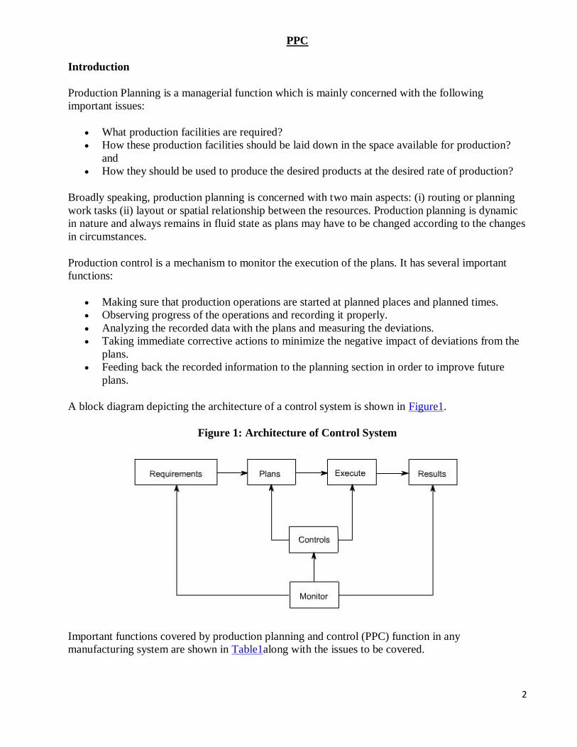
A block diagram depicting the architecture of a control system is shown in Figure1.

Figure 1: Architecture of Control System

Important functions covered by production planning and control (PPC) function in any

manufacturing system are shown in Table1along with the issues to be covered.

3

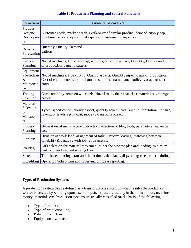
Table 1: Production Planning and control Functions

Functions Issues to be covered

Product

Design&

Developme

nt

Customer needs, market needs, availability of similar product, demand-supply gap,

functional aspects, operational aspects, environmental aspects etc.

Demand

Forecasting

Quantity, Quality, Demand

pattern.

Capacity

Planning

No. of machines, No. of tooling, workers, No.of flow lines, Quantity, Quality and rate

of production, demand pattern.

Equipment

s Selection

&

Maintenan

ce

No. of machines, type of M/c, Quality aspects, Quantity aspects, rate of production,

Cost of equipments, support from the supplier, maintenance policy, storage of spare

parts.

Tooling

Selection

Compactability between w/c steels, No. of tools, their cost, their material etc, storage

policy.

Material

Selection

&

Manageme

nt

Types, specification, quality aspect, quantity aspect, cost, supplies reputation , lot size,

inventory levels, setup cost, mode of transportation etc.

Process

Planning

Generation of manufacture instruction, selection of M/c, tools, parameters, sequence

etc.

Loading Division of work load, assignment of tasks, uniform loading, matching between

capability & capacity with job requirements.

Routing Path selection for material movement as per the process plan and loading, minimum

material handling and waiting time.

Scheduling Time based loading, start and finish times, due dates, dispatching rules, re-scheduling.

Expediting Operation Scheduling and order and progress reporting.

Types of Production Systems

A production system can be defined as a transformation system in which a saleable product or

service is created by working upon a set of inputs. Inputs are usually in the form of men, machine,

money, materials etc. Production systems are usually classified on the basis of the following:

Type of product,

Type of production line,

Rate of production,

Equipments used etc.

4

They are broadly classified into three categories:

Job shop production

Batch production

Mass production

Job Production

In this system products are made to satisfy a specific order. However that order may be produced-

only once

or at irregular time intervals as and when new order arrives

or at regular time intervals to satisfy a continuous demand

The following are the important characteristics of job shop type production system:

Machines and methods employed should be general purpose as product changes are quite

frequent.

Planning and control system should be flexible enough to deal with the frequent changes in

product requirements.

Man power should be skilled enough to deal with changing work conditions.

Schedules are actually non existent in this system as no definite data is available on the

product.

In process inventory will usually be high as accurate plans and schedules do not exist.

Product cost is normally high because of high material and labor costs.

Grouping of machines is done on functional basis (i.e. as lathe section, milling section etc.)

This system is very flexible as management has to manufacture varying product types.

Material handling systems are also flexible to meet changing product requirements.

Batch Production

Batch production is the manufacture of a number of identical articles either to meet a specific order

or to meet a continuous demand. Batch can be manufactured either-

only once

or repeatedly at irregular time intervals as and when demand arise

or repeatedly at regular time intervals to satisfy a continuous demand

The following are the important characteristics of batch type production system:

As final product is somewhat standard and manufactured in batches, economy of scale can be

availed to some extent.

Machines are grouped on functional basis similar to the job shop manufacturing.

Semi automatic, special purpose automatic machines are generally used to take advantage of

the similarity among the products.

Labor should be skilled enough to work upon different product batches.

In process inventory is usually high owing to the type of layout and material handling

policies adopted.

Semi automatic material handling systems are most appropriate in conjunction with the semi

automatic machines.

5

Normally production planning and control is difficult due to the odd size and non repetitive

nature of order.

Mass Production

In mass production, same type of product is manufactured to meet the continuous demand of the

product. Usually demand of the product is very high and market is going to sustain same demand for

sufficiently long time.

The following are the important characteristics of mass production system:

As same product is manufactured for sufficiently long time, machines can be laid down in

order of processing sequence. Product type layout is most appropriate for mass production

system.

Standard methods and machines are used during part manufacture.

Most of the equipments are semi automatic or automatic in nature.

Material handling is also automatic (such as conveyors).

Semi skilled workers are normally employed as most of the facilities are automatic.

As product flows along a pre defined line, planning and control of the system is much easier.

Cost of production is low owing to the high rate of production.

In process inventories are low as production scheduling is simple and can be implemented

with ease.

PRODUCT DESIGN

Product design is a strategic decision as the image and profit earning capacity of a small firm

depends largely on product design. Once the product to be produced is decided by the

entrepreneur the next step is to prepare its design. Product design consists of form and

function. The form designing includes decisions regarding its shape, size, color and

appearance of the product. The functional design involves the working conditions of the

product. Once a product is designed, it prevails for a long time therefore various factors are

to be considered before designing it. These

factors are listed below: -

(a) Standardization

(b) Reliability

(c) Maintainability

(d) Servicing

(e) Reproducibility

(f) Sustainability

(g) Product simplification

(h) Quality Commensuration with cost

(i) Product value

(j) Consumer quality

(k) Needs and tastes of consumers.

6

Above all, the product design should be dictated by the market demand. It is an important

decision and therefore the entrepreneur should pay due effort, time,energy and attention in

order to get the best results.

TYPES OF PRODUCTION SYSTEM

Broadly one can think of three types of production systems which are mentioned

here under: -

(a) Continuous production

(b) Job or unit production

(c) Intermittent production

(a) Continuous production: - It refers to the production of standardized products with a standard set

of process and operation sequence in anticipation of demand. It is also known as mass flow

production or assembly line productionThis system ensures less work in process inventory and high

product quality butinvolves large investment in machinery and equipment. The system is suitable in

117plants involving large volume and small variety of output e.g. oil refineries reform cement

manufacturing etc.

(b) Job or Unit production: - It involves production as per customer's specification each batch or

order consists of a small lot of identical products andis different from other batches. The system

requires comparatively smallerinvestment in machines and equipment. It is flexible and can be

adapted tochanges in product design and order size without much inconvenience. This system is

most suitable where heterogeneous products are produced againstspecific orders.

(c) Intermittent Production: Under this system the goods are produced partly for inventory and

partly for customer's orders. E.g. components are made forinventory but they are combined

differently for different customers. . Automobileplants, printing presses, electrical goods plant are

examples of this type ofmanufacturing.

FORE CASTING

Introduction

The growing competition, frequent changes in customer's demand and the trend towards automation

demand that decisions in business should not be based purely on guesses rather on a careful analysis

of data concerning the future course of events. More time and attention should be given to the future

than to the past, and the question 'what is likely to happen?' should take precedence over 'what has

happened?' though no attempt to answer the first can be made without the facts and figures being

available to answer the second. When estimates of future conditions are made on a systematic basis,

the process is called forecasting and the figure or statement thus obtained is defined as forecast.

In a world where future is not known with certainty, virtually every business and economic decision

rests upon a forecast of future conditions. Forecasting aims at reducing the area of uncertainty that

surrounds management decision-making with respect to costs, profit, sales, production, pricing,

capital investment, and so forth. If the future were known with certainty, forecasting would be

unnecessary. But uncertainty does exist, future outcomes are rarely assured and, therefore, organized

system of forecasting is necessary. The following are the main functions of forecasting:

7

The creation of plans of action.

The general use of forecasting is to be found in monitoring the continuing progress of plans

based on forecasts.

The forecast provides a warning system of the critical factors to be monitored regularly

because they might drastically affect the performance of the plan.

It is important to note that the objective of business forecasting is not to determine a curve or series

of figures that will tell exactly what will happen, say, a year in advance, but it is to make analysis

based on definite statistical data, which will enable an executive to take advantage of future

conditions to a greater extent than he could do without them. In forecasting one should note that it is

impossible to forecast the future precisely and there always must be some range of error allowed for

in the forecast.

FORECASTING FUNDAMENTALS

Forecast: A prediction, projection, or estimate of some future activity, event, or occurrence.

Types of Forecasts

- Economic forecasts

o Predict a variety of economic indicators, like money supply, inflation rates, interest

rates, etc.

- Technological forecasts

o Predict rates of technological progress and innovation.

- Demand forecasts

o Predict the future demand for a company’s products or services.

Since virtually all the operations management decisions (in both the strategic category and the

tactical category) require as input a good estimate of future demand, this is the type of forecasting

that is emphasized in our textbook and in this course.

TYPES OF FORECASTING METHODS

Qualitative methods: These types of forecasting methods are based on judgments, opinions,

intuition, emotions, or personal experiences and are subjective in nature. They do not rely on any

rigorous mathematical computations

Quantitative methods: These types of forecasting methods are based on mathematical

(quantitative) models, and are objective in nature. They rely heavily on mathematical computations.

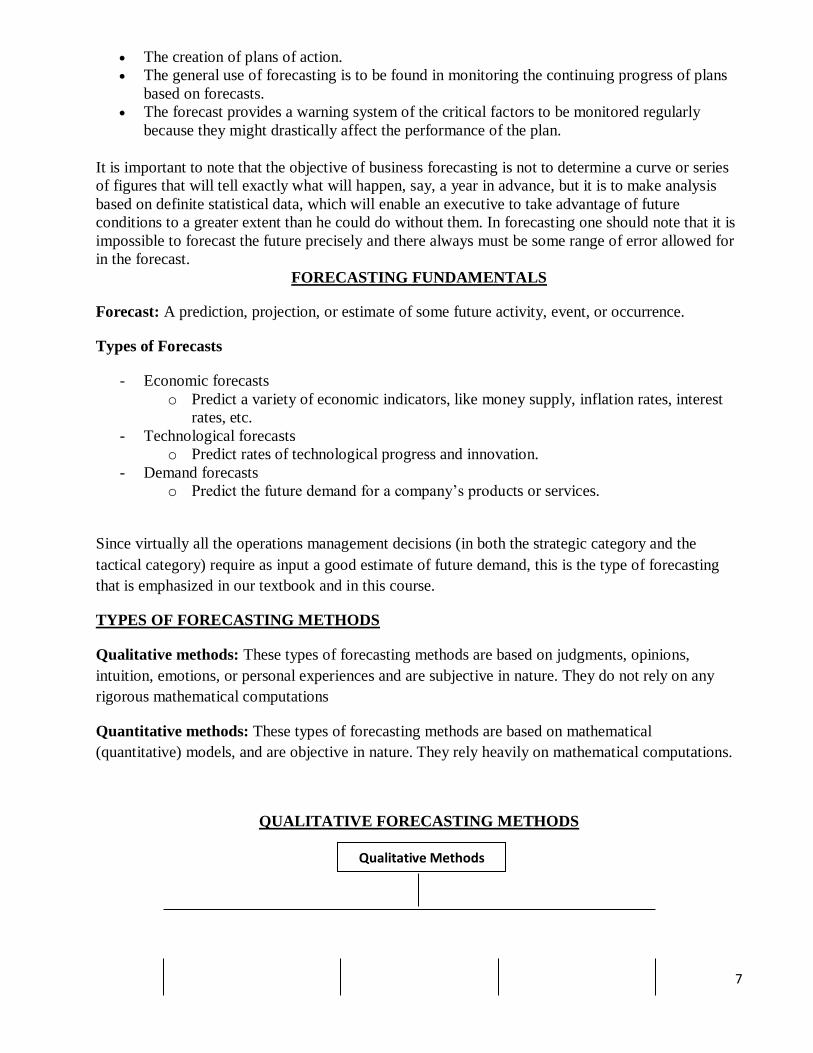
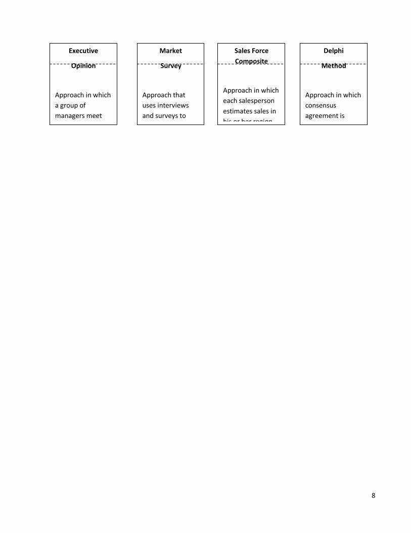
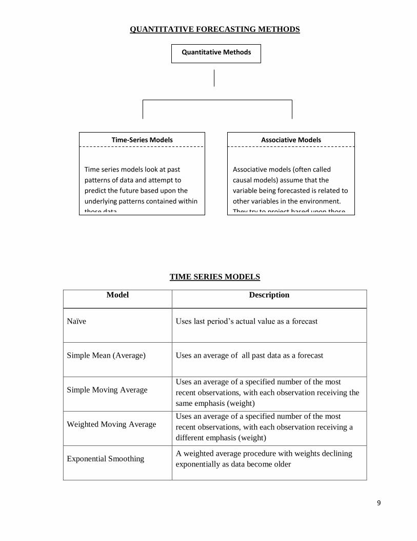
QUALITATIVE FORECASTING METHODS

Qualitative Methods

8

Executive

Opinion

Approach in which

a group of

managers meet

and collectively

develop a forecast

Market

Survey

Approach that

uses interviews

and surveys to

judge preferences

of customer and

to assess demand

Delphi

Method

Approach in which

consensus

agreement is

reached among a

group of experts

Sales Force

Composite

Approach in which

each salesperson

estimates sales in

his or her region

9

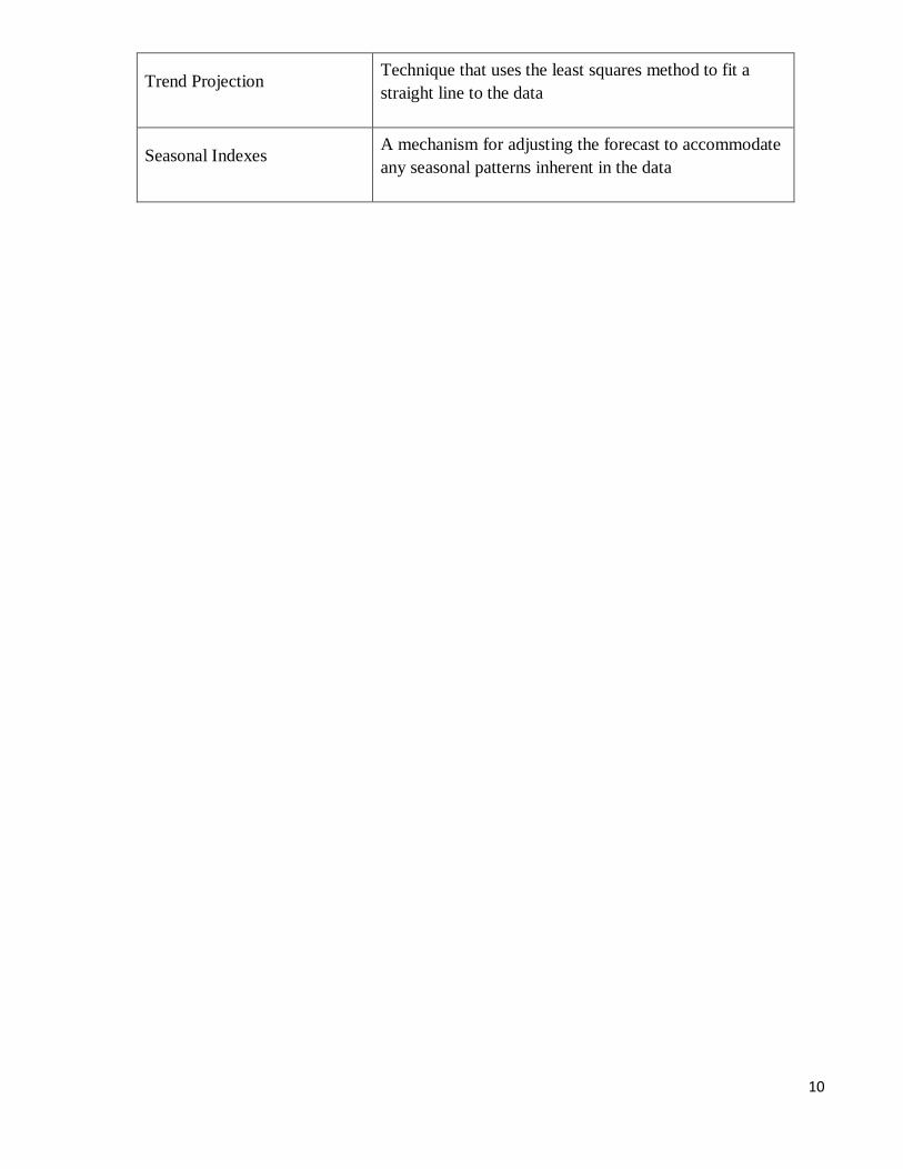
QUANTITATIVE FORECASTING METHODS

TIME SERIES MODELS

Model Description

Naïve Uses last period’s actual value as a forecast

Simple Mean (Average) Uses an average of all past data as a forecast

Simple Moving Average Uses an average of a specified number of the most

recent observations, with each observation receiving the

same emphasis (weight)

Weighted Moving Average Uses an average of a specified number of the most

recent observations, with each observation receiving a

different emphasis (weight)

Exponential Smoothing A weighted average procedure with weights declining

exponentially as data become older

Time-Series Models

Time series models look at past

patterns of data and attempt to

predict the future based upon the

underlying patterns contained within

those data.

Associative Models

Associative models (often called

causal models) assume that the

variable being forecasted is related to

other variables in the environment.

They try to project based upon those

associations.

Quantitative Methods

10

Trend Projection Technique that uses the least squares method to fit a

straight line to the data

Seasonal Indexes A mechanism for adjusting the forecast to accommodate

any seasonal patterns inherent in the data

11

DECOMPOSITION OF A TIME SERIES

Patterns that may be present in a time series

Trend: Data exhibit a steady growth or decline over time.

Seasonality: Data exhibit upward and downward swings in a short to intermediate time frame (most

notably during a year).

Cycles: Data exhibit upward and downward swings in over a very long time frame.

Random variations: Erratic and unpredictable variation in the data over time with no discernable

pattern.

ILLUSTRATION OF TIME SERIES DECOMPOSITION

Hypothetical Pattern of Historical Demand

Dependent versus Independent Demand

Demand of an item is termed as independent when it remains unaffected by the demand for any

other item. On the other hand, when the demand of one item is linked to the demand for another

item, demand is termed as dependent. It is important to mention that only independent demand needs

forecasting. Dependent demand can be derived from the demand of independent item to which it is

linked.

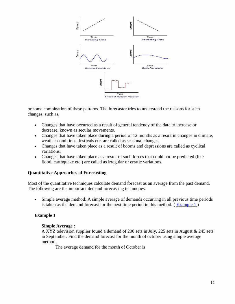
Business Time Series The first step in making a forecast consists of gathering information from the past. One should

collect statistical data recorded at successive intervals of time. Such a data is usually referred to as

time series. Analysts plot demand data on a time scale, study the plot and look for consistent shapes

and patterns. A time series of demand may have constant, trend, or seasonal pattern ( Figure 1 )

Figure 1: Business Time Series

12

or some combination of these patterns. The forecaster tries to understand the reasons for such

changes, such as,

Changes that have occurred as a result of general tendency of the data to increase or

decrease, known as secular movements.

Changes that have taken place during a period of 12 months as a result in changes in climate,

weather conditions, festivals etc. are called as seasonal changes.

Changes that have taken place as a result of booms and depressions are called as cyclical

variations.

Changes that have taken place as a result of such forces that could not be predicted (like

flood, earthquake etc.) are called as irregular or erratic variations.

Quantitative Approaches of Forecasting

Most of the quantitative techniques calculate demand forecast as an average from the past demand.

The following are the important demand forecasting techniques.

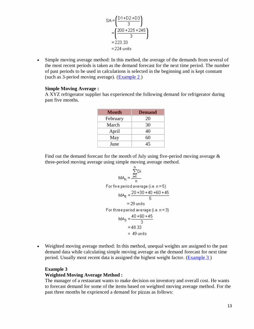
Simple average method: A simple average of demands occurring in all previous time periods

is taken as the demand forecast for the next time period in this method. ( Example 1 )

Example 1

Simple Average :

A XYZ television supplier found a demand of 200 sets in July, 225 sets in August & 245 sets

in September. Find the demand forecast for the month of october using simple average

method.

The average demand for the month of October is

13

Simple moving average method: In this method, the average of the demands from several of

the most recent periods is taken as the demand forecast for the next time period. The number

of past periods to be used in calculations is selected in the beginning and is kept constant

(such as 3-period moving average). (Example 2 )

Simple Moving Average :

A XYZ refrigerator supplier has experienced the following demand for refrigerator during

past five months.

Month Demand

February 20

March 30

April 40

May 60

June 45

Find out the demand forecast for the month of July using five-period moving average &

three-period moving average using simple moving average method.

Weighted moving average method: In this method, unequal weights are assigned to the past

demand data while calculating simple moving average as the demand forecast for next time

period. Usually most recent data is assigned the highest weight factor. (Example 3 )

Example 3

Weighted Moving Average Method :

The manager of a restaurant wants to make decision on inventory and overall cost. He wants

to forecast demand for some of the items based on weighted moving average method. For the

past three months he exprienced a demand for pizzas as follows:

14

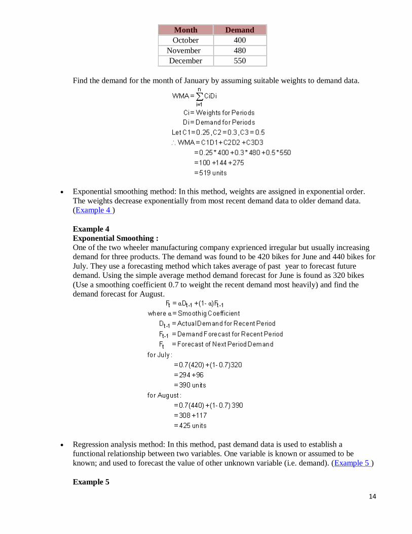
Month Demand

October 400

November 480

December 550

Find the demand for the month of January by assuming suitable weights to demand data.

Exponential smoothing method: In this method, weights are assigned in exponential order.

The weights decrease exponentially from most recent demand data to older demand data.

(Example 4 )

Example 4

Exponential Smoothing :

One of the two wheeler manufacturing company exprienced irregular but usually increasing

demand for three products. The demand was found to be 420 bikes for June and 440 bikes for

July. They use a forecasting method which takes average of past year to forecast future

demand. Using the simple average method demand forecast for June is found as 320 bikes

(Use a smoothing coefficient 0.7 to weight the recent demand most heavily) and find the

demand forecast for August.

Regression analysis method: In this method, past demand data is used to establish a

functional relationship between two variables. One variable is known or assumed to be

known; and used to forecast the value of other unknown variable (i.e. demand). (Example 5 )

Example 5

15

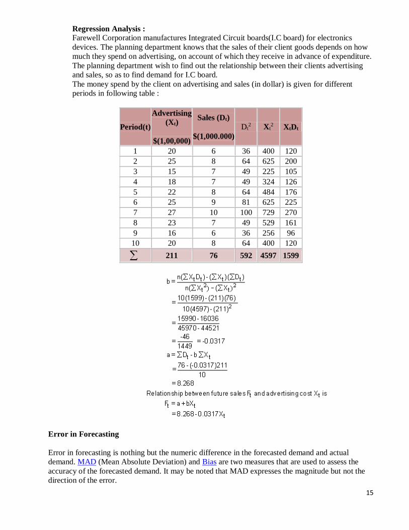
Regression Analysis :

Farewell Corporation manufactures Integrated Circuit boards(I.C board) for electronics

devices. The planning department knows that the sales of their client goods depends on how

much they spend on advertising, on account of which they receive in advance of expenditure.

The planning department wish to find out the relationship between their clients advertising

and sales, so as to find demand for I.C board.

The money spend by the client on advertising and sales (in dollar) is given for different

periods in following table :

Period(t)

Advertising

(Xt)

$(1,00,000)

Sales (Dt)

$(1,000.000)

Dt2 Xt

2 XtDt

1 20 6 36 400 120

2 25 8 64 625 200

3 15 7 49 225 105

4 18 7 49 324 126

5 22 8 64 484 176

6 25 9 81 625 225

7 27 10 100 729 270

8 23 7 49 529 161

9 16 6 36 256 96

10 20 8 64 400 120

211 76 592 4597 1599

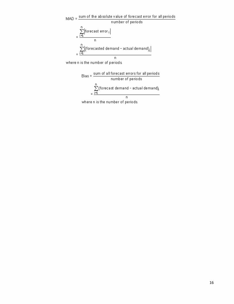
Error in Forecasting

Error in forecasting is nothing but the numeric difference in the forecasted demand and actual

demand. MAD (Mean Absolute Deviation) and Bias are two measures that are used to assess the

accuracy of the forecasted demand. It may be noted that MAD expresses the magnitude but not the

direction of the error.

16

17

INVENTORY

Introduction

The amount of material, a company has in stock at a specific time is known as inventory or in terms

of money it can be defined as the total capital investment over all the materials stocked in the

company at any specific time. Inventory may be in the form of,

raw material inventory

in process inventory

finished goods inventory

spare parts inventory

office stationary etc.

As a lot of money is engaged in the inventories along with their high carrying costs, companies

cannot afford to have any money tied in excess inventories. Any excessive investment in inventories

may prove to be a serious drag on the successful working of an organization. Thus there is a need to

manage our inventories more effectively to free the excessive amount of capital engaged in the

materials.

Why Inventories?

Inventories are needed because demand and supply can not be matched for physical and economical

reasons. There are several other reasons for carrying inventories in any organization.

To safe guard against the uncertainties in price fluctuations, supply conditions, demand

conditions, lead times, transport contingencies etc.

To reduce machine idle times by providing enough in-process inventories at appropriate

locations.

To take advantages of quantity discounts, economy of scale in transportation etc.

To decouple operations i.e. to make one operation's supply independent of another's supply.

This helps in minimizing the impact of break downs, shortages etc. on the performance of the

downstream operations. Moreover operations can be scheduled independent of each other if

operations are decoupled.

To reduce the material handling cost of semi-finished products by moving them in large

quantities between operations.

To reduce clerical cost associated with order preparation, order procurement etc.

Inventory Costs

In order to control inventories appropriately, one has to consider all cost elements that are associated

with the inventories. There are four such cost elements, which do affect cost of inventory.

Unit cost: it is usually the purchase price of the item under consideration. If unit cost is

related with the purchase quantity, it is called as discount price.

Procurement costs: This includes the cost of order preparation, tender placement, cost of

postages, telephone costs, receiving costs, set up cost etc.

18

Carrying costs: This represents the cost of maintaining inventories in the plant. It includes the

cost of insurance, security, warehouse rent, taxes, interest on capital engaged, spoilage,

breakage etc.

Stockout costs: This represents the cost of loss of demand due to shortage in supplies. This

includes cost of loss of profit, loss of customer, loss of goodwill, penalty etc.

If one year planning horizon is used, the total annual cost of inventory can be expressed as:

Total annual inventory cost = Cost of items + Annual procurement cost + Annual carrying

cost + Stockout cost

Variables in Inventory Models

D = Total annual demand (in units)

Q = Quantity ordered (in units)

Q* = Optimal order quantity (in units)

R = Reorder point (in units)

R* = Optimal reorder point (in units)

L = Lead time

S = Procurement cost (per order)

C = Cost of the individual item (cost per unit)

I = Carrying cost per unit carried (as a percentage of unit cost C)

K = Stockout cost per unit out of stock

P = Production rate or delivery rate

dl = Demand per unit time during lead time

Dl = Total demand during lead time

TC = Total annual inventory costs

TC* = Minimum total annual inventory costs

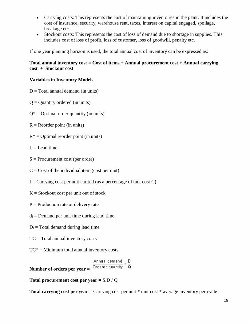
Number of orders per year =

Total procurement cost per year = S.D / Q

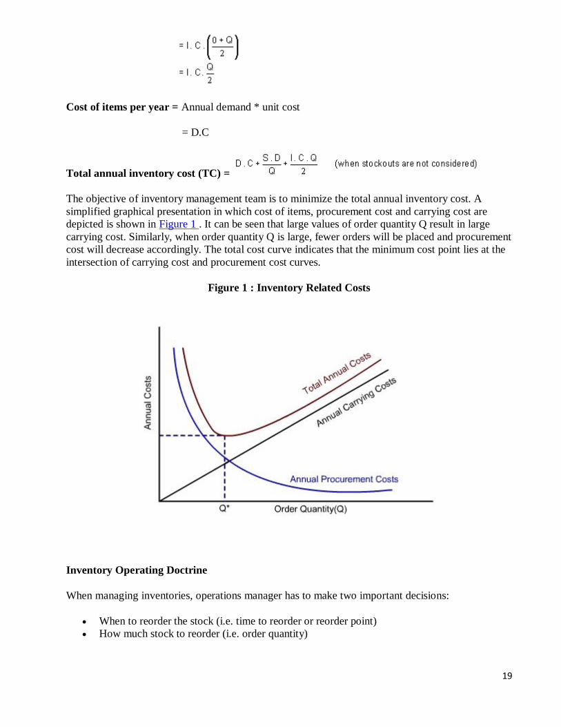
Total carrying cost per year = Carrying cost per unit * unit cost * average inventory per cycle

19

Cost of items per year = Annual demand * unit cost

= D.C

Total annual inventory cost (TC) =

The objective of inventory management team is to minimize the total annual inventory cost. A

simplified graphical presentation in which cost of items, procurement cost and carrying cost are

depicted is shown in Figure 1 . It can be seen that large values of order quantity Q result in large

carrying cost. Similarly, when order quantity Q is large, fewer orders will be placed and procurement

cost will decrease accordingly. The total cost curve indicates that the minimum cost point lies at the

intersection of carrying cost and procurement cost curves.

Figure 1 : Inventory Related Costs

Inventory Operating Doctrine

When managing inventories, operations manager has to make two important decisions:

When to reorder the stock (i.e. time to reorder or reorder point)

How much stock to reorder (i.e. order quantity)

20

Reorder point is usually a predetermined inventory level, which signals the operations manager to

start the procurement process for the next order. Order quantity is the order size.

Inventory Modelling

This is a quantitative approach for deriving the minimum cost model for the inventory problem in

hand.

Economic Order Quantity (EOQ) Model

This model is applied when objective is to minimize the total annual cost of inventory in the

organization. Economic order quantity is that size of the order which helps in attaining the above set

objective. EOQ model is applicable under the following conditions.

Demand per year is deterministic in nature

Planning period is one year

Lead time is zero or constant and deterministic in nature

Replenishment of items is instantaneous

Demand/consumption rate is uniform and known in advance

No stockout condition exist in the organization

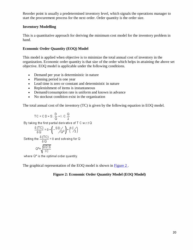
The total annual cost of the inventory (TC) is given by the following equation in EOQ model.

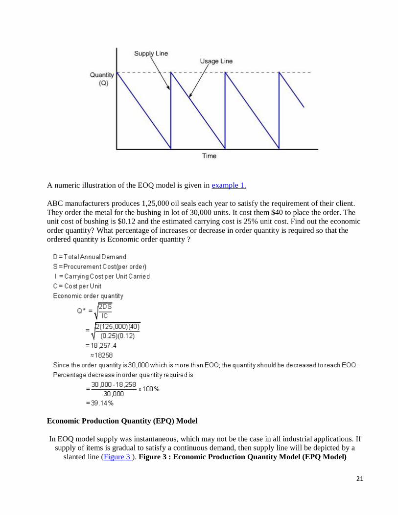
The graphical representation of the EOQ model is shown in Figure 2 .

Figure 2: Economic Order Quantity Model (EOQ Model)

21

A numeric illustration of the EOQ model is given in example 1.

ABC manufacturers produces 1,25,000 oil seals each year to satisfy the requirement of their client.

They order the metal for the bushing in lot of 30,000 units. It cost them $40 to place the order. The

unit cost of bushing is $0.12 and the estimated carrying cost is 25% unit cost. Find out the economic

order quantity? What percentage of increases or decrease in order quantity is required so that the

ordered quantity is Economic order quantity ?

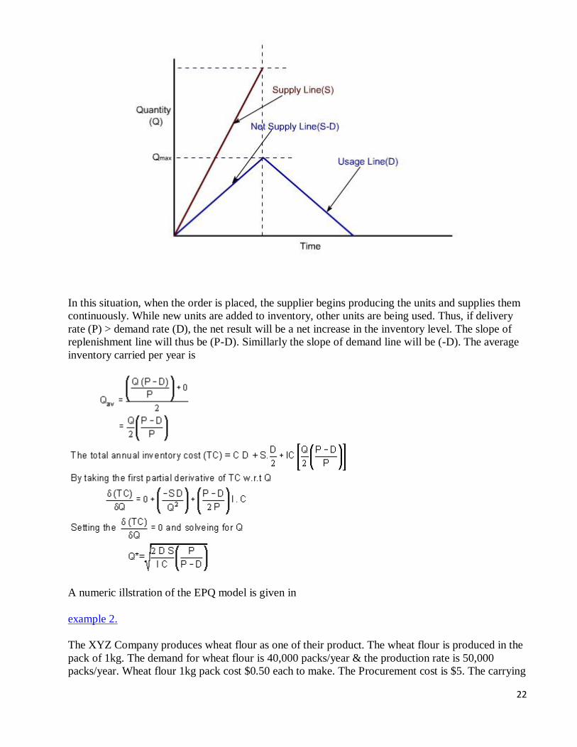
Economic Production Quantity (EPQ) Model

In EOQ model supply was instantaneous, which may not be the case in all industrial applications. If

supply of items is gradual to satisfy a continuous demand, then supply line will be depicted by a

slanted line (Figure 3 ). Figure 3 : Economic Production Quantity Model (EPQ Model)

22

In this situation, when the order is placed, the supplier begins producing the units and supplies them

continuously. While new units are added to inventory, other units are being used. Thus, if delivery

rate (P) > demand rate (D), the net result will be a net increase in the inventory level. The slope of

replenishment line will thus be (P-D). Simillarly the slope of demand line will be (-D). The average

inventory carried per year is

A numeric illstration of the EPQ model is given in

example 2.

The XYZ Company produces wheat flour as one of their product. The wheat flour is produced in the

pack of 1kg. The demand for wheat flour is 40,000 packs/year & the production rate is 50,000

packs/year. Wheat flour 1kg pack cost $0.50 each to make. The Procurement cost is $5. The carrying

23

cost is high because the product gets spoiled in few week times span. It is nearly 50 percent of cost

of one pack. Find out the operating doctrine.

MRP

Introduction

It was discussed in demand forecasting that in the dependent demand situation, if the demand for an

item is known, the demand for other related items can be deduced. For example, if the demand of an

automobile is known, the demand of its sub assemblies and sub components can easily be deduced.

For dependent demand situations, normal reactive inventory control systems (i.e. EOQ etc.) are not

suitable because they result in high inventory costs and unreliable delivery schedules. More recently,

managers have realized that inventory planning systems (such as materials requirements planning)

are better suited for dependent demand items. MRP is a simple system of calculating arithmetically

the requirements of the input materials at different points of time based on actual production plan.

MRP can also be defined as a planning and scheduling system to meet time-phased materials

requirements for production operations. MRP always tries to meet the delivery schedule of end

products as specified in the master production schedule.

MRP Objectives

MRP has several objectives, such as:

Reduction in Inventory Cost: By providing the right quantity of material at right time to

meet master production schedule, MRP tries to avoid the cost of excessive inventory.

24

Meeting Delivery Schedule: By minimizing the delays in materials procurement, production

decision making, MRP helps avoid delays in production thereby meeting delivery schedules

more consistently.

Improved Performance: By stream lining the production operations and minimizing the

unplanned interruptions, MRP focuses on having all components available at right place in

right quantity at right time.

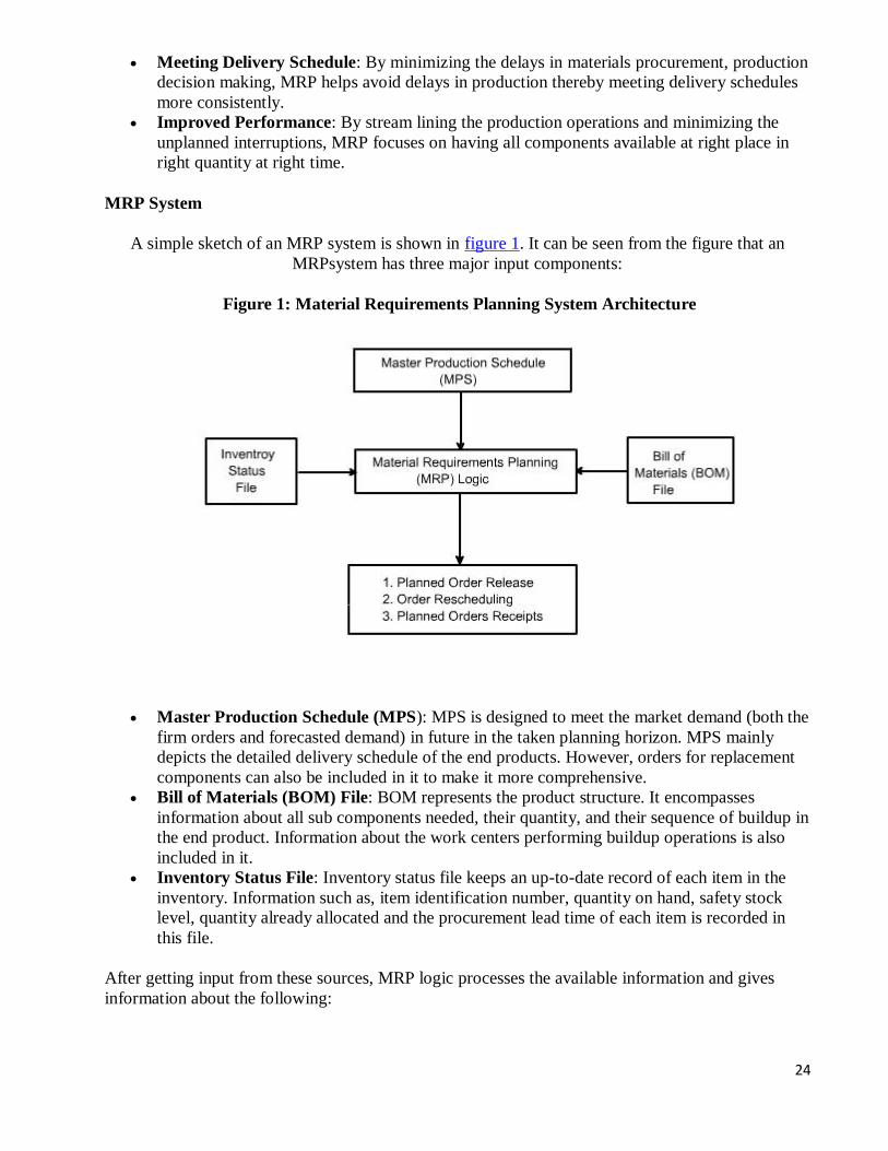
MRP System

A simple sketch of an MRP system is shown in figure 1. It can be seen from the figure that an

MRPsystem has three major input components:

Figure 1: Material Requirements Planning System Architecture

Master Production Schedule (MPS): MPS is designed to meet the market demand (both the

firm orders and forecasted demand) in future in the taken planning horizon. MPS mainly

depicts the detailed delivery schedule of the end products. However, orders for replacement

components can also be included in it to make it more comprehensive.

Bill of Materials (BOM) File: BOM represents the product structure. It encompasses

information about all sub components needed, their quantity, and their sequence of buildup in

the end product. Information about the work centers performing buildup operations is also

included in it.

Inventory Status File: Inventory status file keeps an up-to-date record of each item in the

inventory. Information such as, item identification number, quantity on hand, safety stock

level, quantity already allocated and the procurement lead time of each item is recorded in

this file.

After getting input from these sources, MRP logic processes the available information and gives

information about the following:

25

Planned Orders Receipts: This is the order quantity of an item that is planned to be ordered

so that it is received at the beginning of the period under consideration to meet the net

requirements of that period. This order has not yet been placed and will be placed in future.

Planned Order Release: This is the order quantity of an item that is planned to be ordered in

the planned time period for this order that will ensure that the item is received when needed.

Planned order release is determined by offsetting the planned order receipt by procurement

lead time of that item.

Order Rescheduling: This highlight the need of any expediting, de-expediting, and

cancellation of open orders etc. in case of unexpected situations.

CPM

Project Management

A project is a well defined task which has a definable beginning and a definable end and requires

one or more resources for the completion of its constituent activities, which are interrelated and

which must be accomplished to achieve the objectives of the project. Project management is evolved

to coordinate and control all project activities in an efficient and cost effective manner. The salient

features of a project are:

A project has identifiable beginning and end points.

Each project can be broken down into a number of identifiable activities which will consume

time and other resources during their completion.

A project is scheduled to be completed by a target date.

A project is usually large and complex and has many interrelated activities.

The execution of the project activities is always subjected to some uncertainties and risks.

Network Techniques

The network techniques of project management have developed in an evolutionary way in many

years. Up to the end of 18th century, the decision making in general and project management in

particular was intuitive and depended primarily on managerial capabilities, experience, judgment

and academic background of the managers. It was only in the early of 1900's that the pioneers of

scientific management, started developing the scientific management techniques. The forerunner to

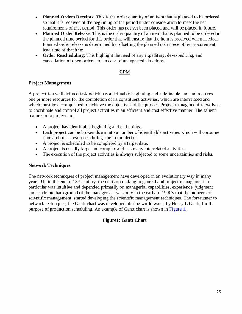
network techniques, the Gantt chart was developed, during world war I, by Henry L Gantt, for the

purpose of production scheduling. An example of Gantt chart is shown in Figure 1.

Figure1: Gantt Chart

26

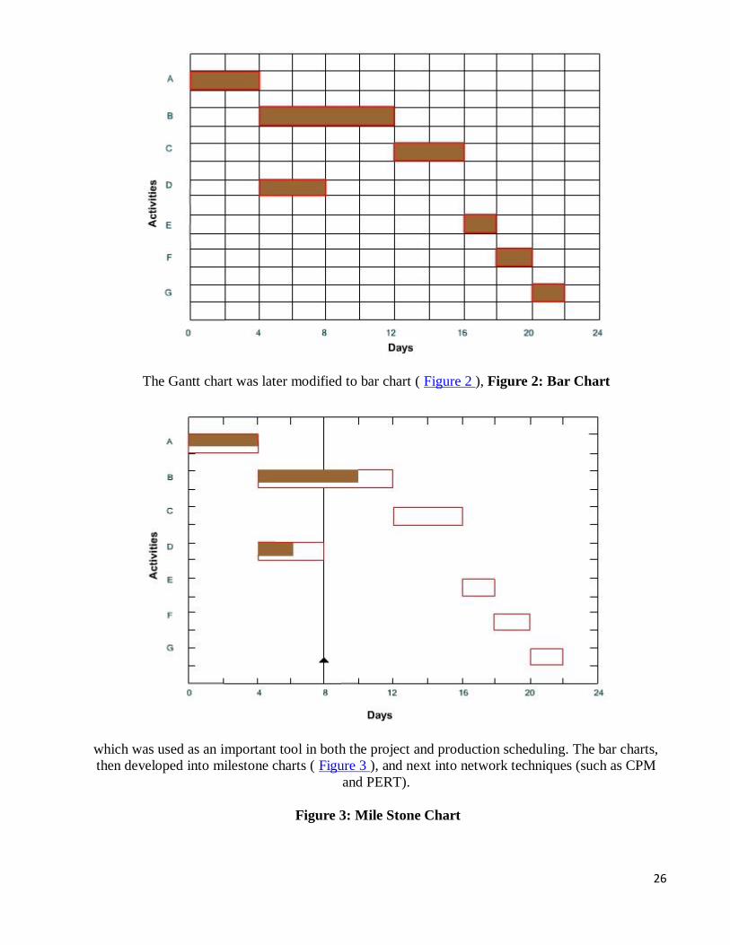
The Gantt chart was later modified to bar chart ( Figure 2 ), Figure 2: Bar Chart

which was used as an important tool in both the project and production scheduling. The bar charts,

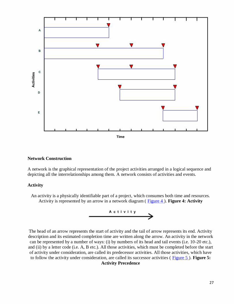
then developed into milestone charts ( Figure 3 ), and next into network techniques (such as CPM

and PERT).

Figure 3: Mile Stone Chart

27

Network Construction

A network is the graphical representation of the project activities arranged in a logical sequence and

depicting all the interrelationships among them. A network consists of activities and events.

Activity

An activity is a physically identifiable part of a project, which consumes both time and resources.

Activity is represented by an arrow in a network diagram ( Figure 4 ). Figure 4: Activity

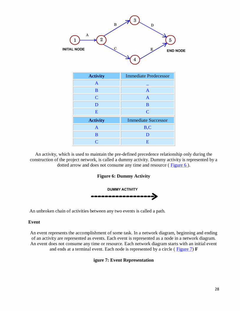
The head of an arrow represents the start of activity and the tail of arrow represents its end. Activity

description and its estimated completion time are written along the arrow. An activity in the network

can be represented by a number of ways: (i) by numbers of its head and tail events (i.e. 10-20 etc.),

and (ii) by a letter code (i.e. A, B etc.). All those activities, which must be completed before the start

of activity under consideration, are called its predecessor activities. All those activities, which have

to follow the activity under consideration, are called its successor activities ( Figure 5 ). Figure 5:

Activity Precedence

28

Activity Immediate Predecessor

A _

B A

C A

D B

E C

Activity Immediate Successor

A B,C

B D

C E

An activity, which is used to maintain the pre-defined precedence relationship only during the

construction of the project network, is called a dummy activity. Dummy activity is represented by a

dotted arrow and does not consume any time and resource ( Figure 6 ).

Figure 6: Dummy Activity

An unbroken chain of activities between any two events is called a path.

Event

An event represents the accomplishment of some task. In a network diagram, beginning and ending

of an activity are represented as events. Each event is represented as a node in a network diagram.

An event does not consume any time or resource. Each network diagram starts with an initial event

and ends at a terminal event. Each node is represented by a circle ( Figure 7) F

igure 7: Event Representation

29

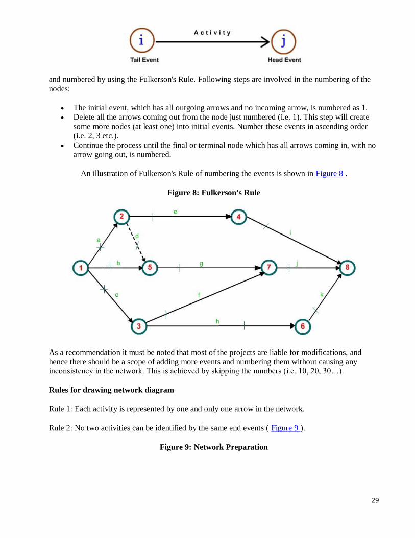
and numbered by using the Fulkerson's Rule. Following steps are involved in the numbering of the

nodes:

The initial event, which has all outgoing arrows and no incoming arrow, is numbered as 1.

Delete all the arrows coming out from the node just numbered (i.e. 1). This step will create

some more nodes (at least one) into initial events. Number these events in ascending order

(i.e. 2, 3 etc.).

Continue the process until the final or terminal node which has all arrows coming in, with no

arrow going out, is numbered.

An illustration of Fulkerson's Rule of numbering the events is shown in Figure 8 .

Figure 8: Fulkerson's Rule

As a recommendation it must be noted that most of the projects are liable for modifications, and

hence there should be a scope of adding more events and numbering them without causing any

inconsistency in the network. This is achieved by skipping the numbers (i.e. 10, 20, 30…).

Rules for drawing network diagram

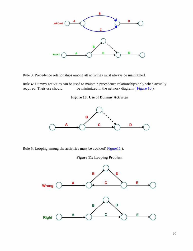
Rule 1: Each activity is represented by one and only one arrow in the network.

Rule 2: No two activities can be identified by the same end events ( Figure 9 ).

Figure 9: Network Preparation

30

Rule 3: Precedence relationships among all activities must always be maintained.

Rule 4: Dummy activities can be used to maintain precedence relationships only when actually

required. Their use should be minimized in the network diagram ( Figure 10 ).

Figure 10: Use of Dummy Activites

Rule 5: Looping among the activities must be avoided( Figure11 ).

Figure 11: Looping Problem

31

CPM and PERT

The CPM (critical path method) system of networking is used, when the activity time estimates are

deterministic in nature. For each activity, a single value of time, required for its execution, is

estimated. Time estimates can easily be converted into cost data in this technique. CPM is an activity

oriented technique.

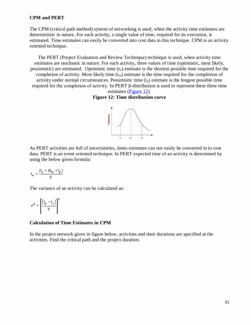
The PERT (Project Evaluation and Review Technique) technique is used, when activity time

estimates are stochastic in nature. For each activity, three values of time (optimistic, most likely,

pessimistic) are estimated. Optimistic time (to) estimate is the shortest possible time required for the

completion of activity. Most likely time (tm) estimate is the time required for the completion of

activity under normal circumstances. Pessimistic time (tp) estimate is the longest possible time

required for the completion of activity. In PERT β-distribution is used to represent these three time

estimates (Figure 12).

Figure 12: Time distribution curve

As PERT activities are full of uncertainties, times estimates can not easily be converted in to cost

data. PERT is an event oriented technique. In PERT expected time of an activity is determined by

using the below given formula:

The variance of an activity can be calculated as:

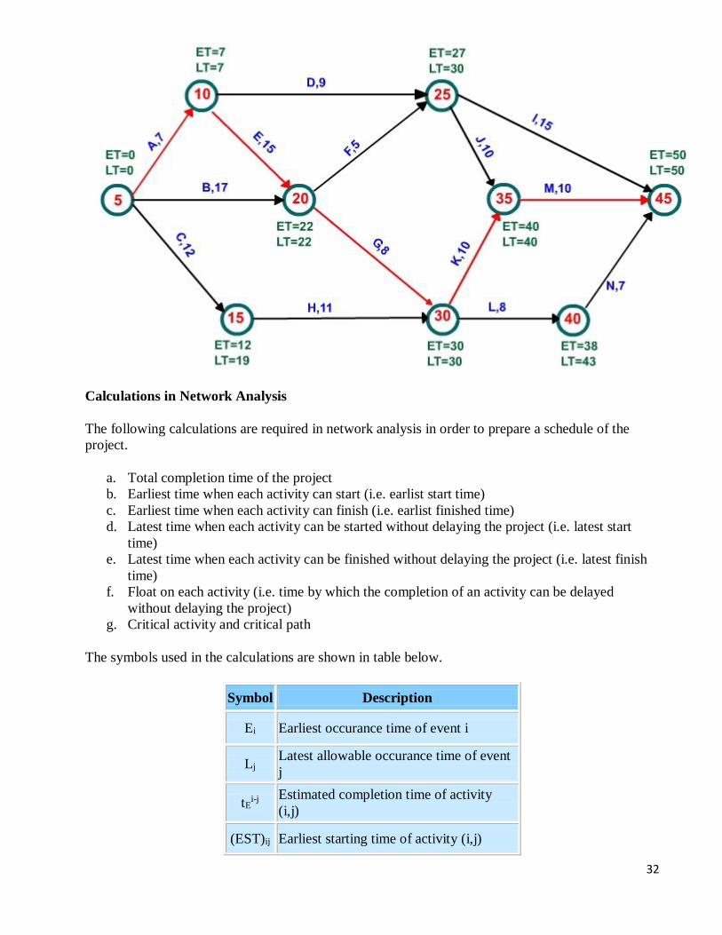
Calculation of Time Estimates in CPM

In the project network given in figure below, activities and their durations are specified at the

activities. Find the critical path and the project duration.

32

Calculations in Network Analysis

The following calculations are required in network analysis in order to prepare a schedule of the

project.

a. Total completion time of the project

b. Earliest time when each activity can start (i.e. earlist start time)

c. Earliest time when each activity can finish (i.e. earlist finished time)

d. Latest time when each activity can be started without delaying the project (i.e. latest start

time)

e. Latest time when each activity can be finished without delaying the project (i.e. latest finish

time)

f. Float on each activity (i.e. time by which the completion of an activity can be delayed

without delaying the project)

g. Critical activity and critical path

The symbols used in the calculations are shown in table below.

Symbol Description

Ei Earliest occurance time of event i

Lj Latest allowable occurance time of event

j

tEi-j

Estimated completion time of activity

(i,j)

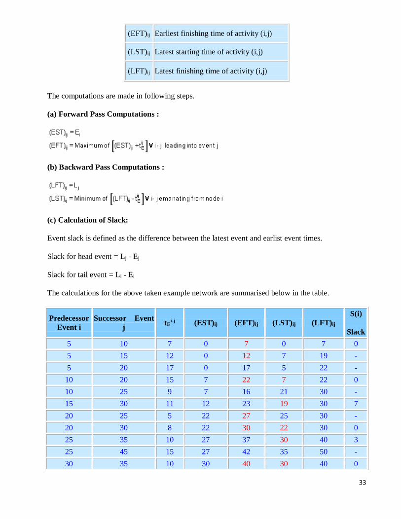
(EST)ij Earliest starting time of activity (i,j)

33

(EFT)ij Earliest finishing time of activity (i,j)

(LST)ij Latest starting time of activity (i,j)

(LFT)ij Latest finishing time of activity (i,j)

The computations are made in following steps.

(a) Forward Pass Computations :

(b) Backward Pass Computations :

(c) Calculation of Slack:

Event slack is defined as the difference between the latest event and earlist event times.

Slack for head event = Lj - Ej

Slack for tail event = Li - Ei

The calculations for the above taken example network are summarised below in the table.

Predecessor

Event i

Successor Event

j tE

i-j (EST)ij (EFT)ij (LST)ij (LFT)ij

S(i)

Slack

5 10 7 0 7 0 7 0

5 15 12 0 12 7 19 -

5 20 17 0 17 5 22 -

10 20 15 7 22 7 22 0

10 25 9 7 16 21 30 -

15 30 11 12 23 19 30 7

20 25 5 22 27 25 30 -

20 30 8 22 30 22 30 0

25 35 10 27 37 30 40 3

25 45 15 27 42 35 50 -

30 35 10 30 40 30 40 0

34

30 40 8 30 38 35 43 -

35 45 10 40 50 40 50 0

40 45 7 38 45 43 50 5

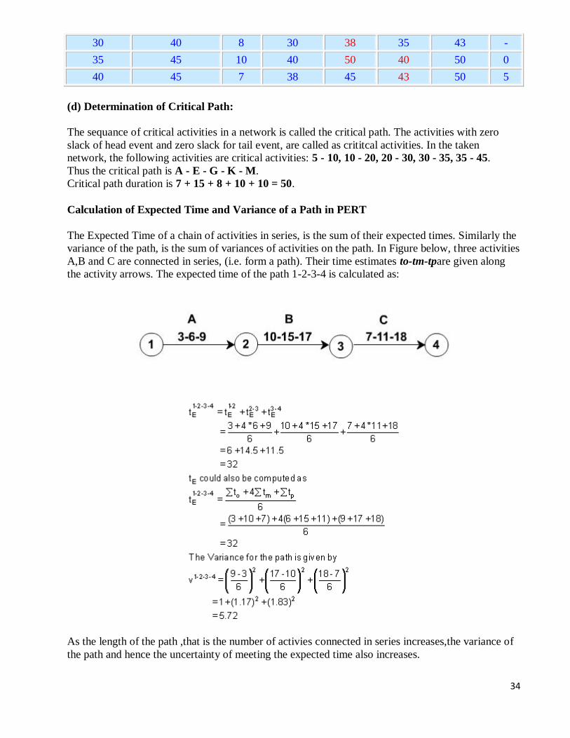
(d) Determination of Critical Path:

The sequance of critical activities in a network is called the critical path. The activities with zero

slack of head event and zero slack for tail event, are called as crititcal activities. In the taken

network, the following activities are critical activities: 5 - 10, 10 - 20, 20 - 30, 30 - 35, 35 - 45.

Thus the critical path is A - E - G - K - M.

Critical path duration is 7 + 15 + 8 + 10 + 10 = 50.

Calculation of Expected Time and Variance of a Path in PERT

The Expected Time of a chain of activities in series, is the sum of their expected times. Similarly the

variance of the path, is the sum of variances of activities on the path. In Figure below, three activities

A,B and C are connected in series, (i.e. form a path). Their time estimates to-tm-tpare given along

the activity arrows. The expected time of the path 1-2-3-4 is calculated as:

As the length of the path ,that is the number of activies connected in series increases,the variance of

the path and hence the uncertainty of meeting the expected time also increases.

35

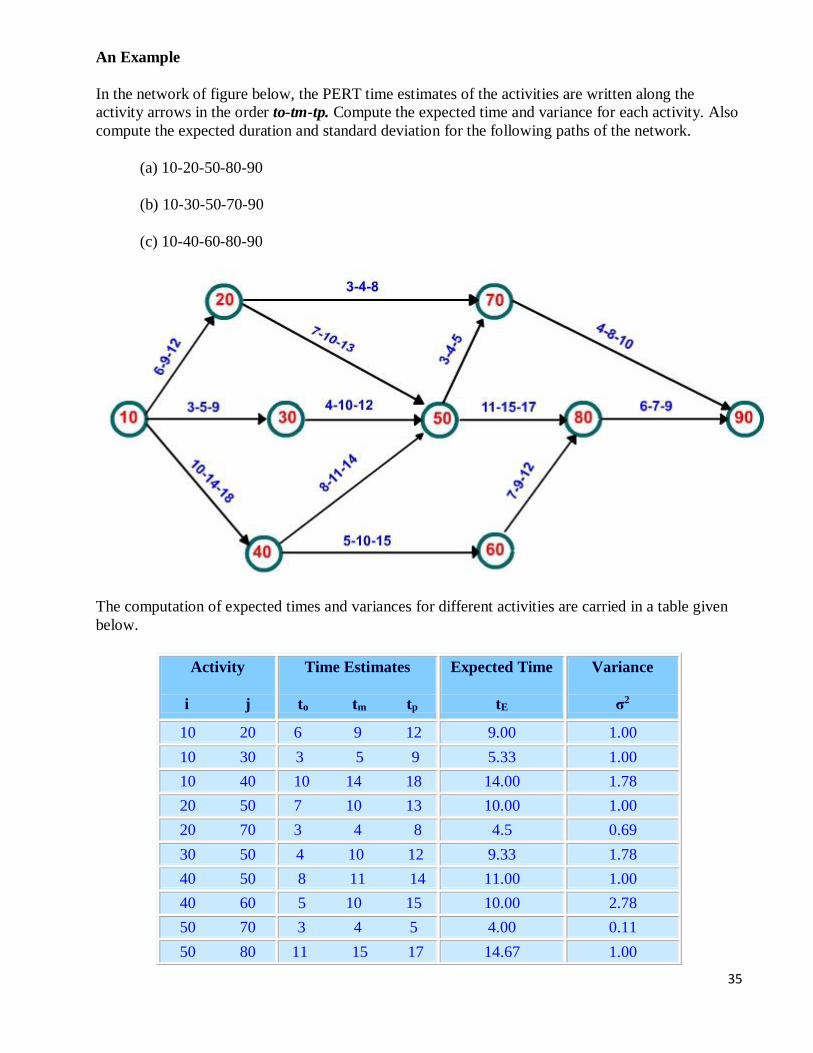
An Example

In the network of figure below, the PERT time estimates of the activities are written along the

activity arrows in the order to-tm-tp. Compute the expected time and variance for each activity. Also

compute the expected duration and standard deviation for the following paths of the network.

(a) 10-20-50-80-90

(b) 10-30-50-70-90

(c) 10-40-60-80-90

The computation of expected times and variances for different activities are carried in a table given

below.

Activity

i j

Time Estimates

to tm tp

Expected Time

tE

Variance

σ2

10 20 6 9 12 9.00 1.00

10 30 3 5 9 5.33 1.00

10 40 10 14 18 14.00 1.78

20 50 7 10 13 10.00 1.00

20 70 3 4 8 4.5 0.69

30 50 4 10 12 9.33 1.78

40 50 8 11 14 11.00 1.00

40 60 5 10 15 10.00 2.78

50 70 3 4 5 4.00 0.11

50 80 11 15 17 14.67 1.00

36

60 80 7 9 12 9.17 0.69

70 90 4 8 10 7.67 1.00

80 90 6 7 9 7.17 0.25