Unit-I

1. Introduction

o Differences between fluid and solid

o Differences between gas and liquid

2. Types of fluids:

o Newtonian & non-Newtonian fluids

o Compressible & incompressible fluids

3. Physical properties:

o Viscosity

o Vapor pressure

o Compressibility and Bulkmodulus

o Surface tension

o Capillarity

o Problems - SurfaceTension

4. Fluid statics:

o Pascal's law for pressure at a pointin a fluid

o Variation of pressure in a Static fluid

o Absolute and gauge pressure,vacuum

5. Pressure Measurement

o Fluid Pressure

o Barometers

o Piezo meters

o Manometers:

Introduction

Simple U-tube manometer

Inverted U-tube manometer

Manometer with one leg enlarged

Two fluid U-tube manometer

Inclined U-tube manometer

Manometer - limitations

o Pressure gauges - Bourdon gauge

6. Buoyancy - principles

7. Units and Dimensions

8. Similitude and model studies:

o Kinematic and dynamic similarities

o DimensionalAnalysis:

o Rayleigh's method

o Buckingham pi method

o Important DimensionlessNumbers

Unit -II

1. Fluid flow:

o Stream line

o Stream tube

o Steady & Uniform flows

o One-dimensional & multidimensional flow

o Equation of continuity

o Energy equation - Bernoulli's equation

Tank training problem

o Momentum equation

o Toricellie equation

o Trajectory of a liquid-jet issued upwards in the atmosphere

o Trajectory of a jet issued from an orifice at the side of a tank

o Water Hammer

o Laminar and Turbulent flow

2. Boundary layer concepts:

o Introduction

o Development of boundary layer for flow over a flat plate

o Development of boundary layer for flow through circular pipe

o Entry length

o Fully developed flow

o Boundary layer separation

3. Flow of incompressible fluid in pipes:

o Laminar flow

o Hagen Poiseuille equation

o Friction factor

o Pressure drop in turbulent flow

o Velocity Distribution for turbulent flow

o Surface roughness

o Flow through non-circular pipes

o Flow through curved pipes

o Expansion losses

o Contraction losses

o Losses for flow through fittings

o Equivalent length of pipe fittings

4. Types of flow problems

5. Compressible fluid flow:

o Equations of compressible flow

o Velocity of sound in fluid

o Mach number

o Nozzles & diffusers

o Maximum velocity

6. Two dimensional flow:

o Velocity potential

o Potential function

o Irrotational flow

Unit -III

1. Closed channel flow measurement:

o Venturi meter

o Orifice meter

o Venturi - Orifice Comparison

o Pitot tube

o Rotameter

o Flow measurement based on Doppler effect

o Hot wire and hot film anemometer

o Magnetic flow meter

2. Open channel flow measurement:

o Elementary theory of weirs and notches

o Rectangular notch

o V-notch

o Suppressed and contracted weirs

o Submerged weirs

o Trapezoidal notch

Unit -IV

1. Flow past immersed bodies:

o Form drag

o Wall drag

o Drag coefficients

2. Friction in flow through bed of solids:

o Blake-Kozeny Equation

o Burke-Plummer Equation

o Ergun equation

3. Packed Towers:

o Applications

o Various types of packing

o Requirements for a good packing

o Loading and Flooding

4. Fluidization:

o Minimum fluidizing velocity

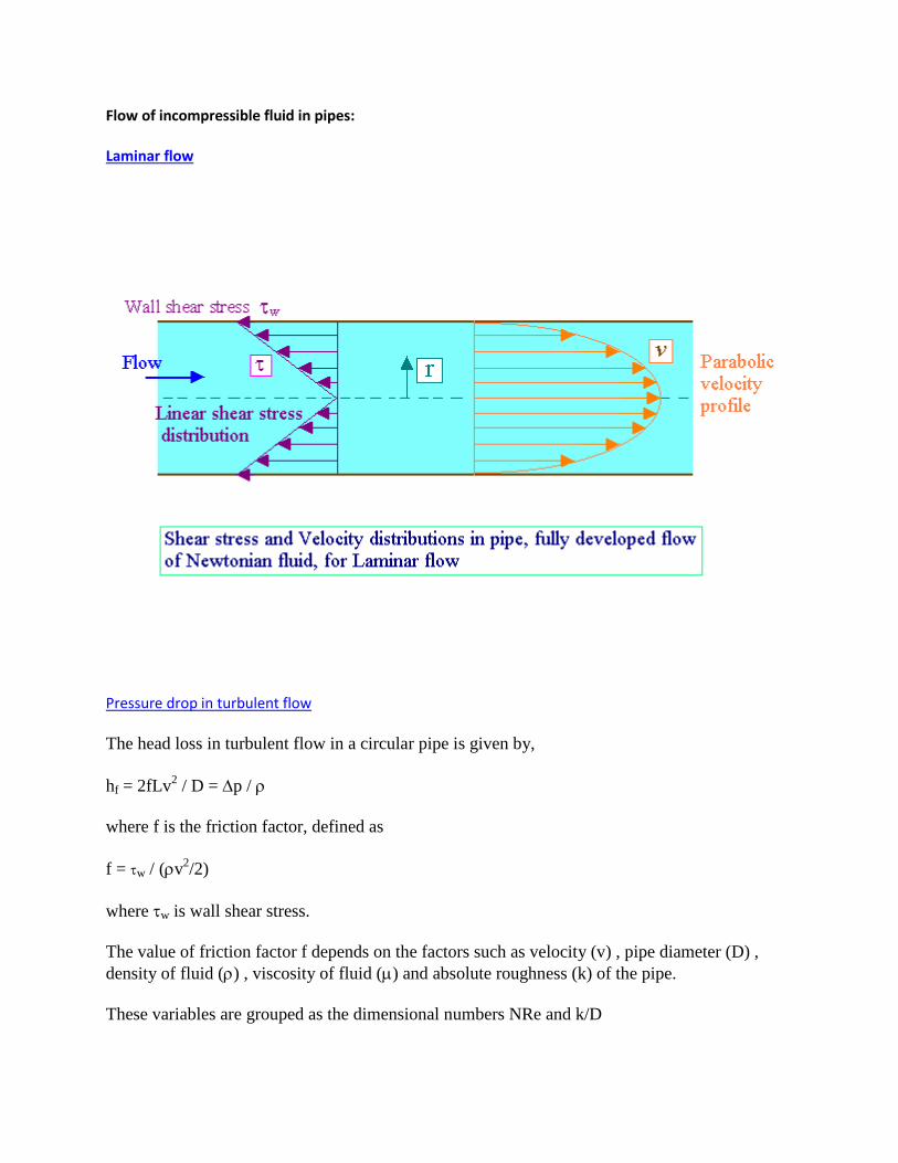
o Pressure Drop in Fluidized bed

o Fluidization Types

5. Motion of particle through fluid

6. Terminal settling velocity

7. Operating ranges of fluidization

8. Applications of fluidization

9. Pneumatic transport

Unit -V

1. Transportation of fluids:

o Pump classifications:

o Suction, discharge , net pressure heads, specific speed and power calculations

o NPSH

2. Characteristics and constructional details of centrifugal pumps

o Cavitation

o Priming

3. Positive displacement pumps:

o Piston pumps - single and double acting

o Plunger pumps

o Diaphragm pump

4. Rotary pumps

o Gear pumps

o Lobe pumps

o Screw pumps

5. Airlift pump

6. Jet pump

7. Selection of pumps

8. Fans, blowers, and compressors

Appendix

Key Contributors to Fluid Mechanics

Fluid Mechanicsis that section of applied mechanics, concerned with the statics and dynamics of

liquids and gases.

A knowledge of fluid mechanics is essential for the chemical engineer, because the majority of

chemical processing operations are conducted either partially or totally in the fluid phase.

The handling of liquids is much simpler, much cheaper, and much less troublesome than

handling solids.

Even in many operations a solid is handled in a finely divided state so that it stays in suspension

in a fluid.

Fluid Statics: Which treats fluids in the equilibrium state of no shear stress

Fluid Mechanics: Which treats when portions of fluid are in motion relative to other parts.

Fluids and their Properties

Fluids

In everyday life, we recognize three states of matter:solid,liquid and gas. Although different in

many respects, liquids and gases have a common characteristic in which they differ from solids:

they are fluids, lacking the ability of solids to offer a permanent resistance to a deforming force.

A fluid is a substance which deforms continuously under the action of shearing forces, however

small they may be.Conversely, it follows that:

If a fluid is at rest, there can be no shearing forces acting and, therefore, all forces in the fluid

must be perpendicular to the planes upon which they act.

Shear stress in a moving fluid

Although there can be no shear stress in a fluid at rest, shear stresses are developed when the

fluid is in motion, if the particles of the fluid move relative to each other so that they have

different velocities, causing the original shape of the fluid to become distorted. If, on the other

hand, the velocity of the fluid is same at every point, no shear stresses will be produced, since the

fluid particles are at rest relative to each other.

Differences between fluid and solid :

The differences between the behaviours of solids and fluids under an applied force are as

follows:

i. For a solid, the strain is a function of the applied stress, providing that the elastic limit is

not exceeded. For a fluid, the rate of strain is proportional to the applied stress.

ii. The strain in a solid is independent of the time over which the force is applied and, if the

elastic limit is not exceeded, the deformation disappears when the force is removed. A

fluid continues to flow as long as the force is applied and will not recover its original

form when the force is removed.

Differences between gas and liquid:

Although liquids and gases both share the common characteristics of fluids, they have many

distinctive characteristics of their own. A liquid is difficult to compress and, for many purposes,

may be regarded as incompressible. A given mass of liquid occupies a fixed volume, irrespective

of the size or shape of its container, and a free surface is formed if the volume of the container is

greater than that of the liquid.

A gas is comparatively easy to compress. Changes of volume with pressure are large, cannot

normally be neglected and are related to changes of temperature. A given mass of gas has no

fixed volume and will expand continuously unless restrained by a containing vessel. It will

completely fill any vessel in which it is placed and, therefore, does not form a free surface.

Types of fluids:

Newtonian & non-Newtonian fluids:

Newtonian fluids:

Fluids which obey the Newton's law of viscosity are called as Newtonian fluids. Newton's law of

viscosity is given by

= dv/dy

where = shear stress

= viscosity of fluid

dv/dy = shear rate, rate of strain or velocity gradient

All gases and most liquids which have simpler molecular formula and low molecular weight

such as water, benzene, ethyl alcohol, CCl4, hexane and most solutions of simple molecules are

Newtonian fluids.

Non-Newtonian fluids:

Fluids which do not obey the Newton's law of viscosity are called as non-Newtonian fluids.

Generally non-Newtonian fluids are complex mixtures: slurries, pastes, gels, polymer solutions

etc.,

Various non-Newtonian Behaviors:

Time-Independent behaviors:

Properties are independent of time under shear.

Bingham-plastic: Resist a small shear stress but flow easily under larger shear stresses. e.g.

tooth-paste, jellies, and some slurries.

Pseudo-plastic: Most non-Newtonian fluids fall into this group. Viscosity decreases with

increasing velocity gradient. e.g. polymer solutions, blood. Pseudoplastic fluids are also called as

Shear thinning fluids. At low shear rates(du/dy) the shear thinning fluid is more viscous than the

Newtonian fluid, and at high shear rates it is less viscous.

Dilatant fluids: Viscosity increases with increasing velocity gradient. They are uncommon, but

suspensions of starch and sand behave in this way. Dilatant fluids are also called as shear

thickening fluids.

Time dependent behaviors:

Those which are dependent upon duration of shear.

Thixotropic fluids: for which the dynamic viscosity decreases with the time for which shearing

forces are applied. e.g. thixotropic jelly paints.

Rheopectic fluids: Dynamic viscosity increases with the time for which shearing forces are

applied. e.g. gypsum suspension in water.

Visco-elastic fluids: Some fluids have elastic properties, which allow them to spring back when

a shear force is released. e.g. egg white.

Compressible & incompressible fluids

Physical properties:

Viscosity:

The viscosity () of a fluid measures its resistance to flow under an applied shear stress.

Representative units for viscosity are kg/(m.sec), g/(cm.sec) (also known as poise designated by

P). The centipoise (cP), one hundredth of a poise, is also a convenient unit, since the viscosity of

water at room temperature is approximately 1 centipoise.

The kinematic viscosity () is the ratio of the viscosity to the density:

= /

and will be found to be important in cases in which significant viscous and gravitational forces

exist.

Viscosity of liquids:

Viscosity of liquids in general, decreases with increasing temperature.

The viscosities () of liquids generally vary approximately with absolute temperature T

according to:

ln = a - b ln T

Viscosity of gases:

Viscosity of gases increases with increase in temperature.

The viscosity () of many gases is approximated by the formula:

= o(T/To)n

in which T is the absolute temperature, o is the viscosity at an absolute reference temperature

To, and n is an empirical exponent that best fits the experimental data.

The viscosity of an ideal gas is independent of pressure, but the viscosities of real gases and

liquids usually increase with pressure.

Viscosity of liquids are generally two orders of magnitude greater than gases at atmospheric

pressure. Fow example, at 25oC, water = 1 centipoise and air = 1 x 10

-2centipoise.

Vapor pressure:

The pressure at which a liquid will boil is called its vapor pressure. This pressure is a function of

temperature (vapor pressure increases with temperature). In this context we usually think about the

temperature at which boiling occurs. For example, water boils at 100oC at sea-level atmospheric

pressure (1 atm abs). However, in terms of vapor pressure, we can say that by increasing the

temperature of water at sea level to 100 oC, we increase the vapor pressure to the point at which it is

equal to the atmospheric pressure (1 atm abs), so that boiling occurs. It is easy to visualize that boiling

can also occur in water at temperatures much below 100oC if the pressure in the water is reduced to its

vapor pressure. For example, the vapor pressure of water at 10oC is 0.01 atm. Therefore, if the pressure

within water at that temperature is reduced to that value, the water boils. Such boiling often occurs in

flowing liquids, such as on the suction side of a pump. When such boiling does occur in the flowing

liquids, vapor bubbles start growing in local regions of very low pressre and then collapse in regions of

high downstream pressure. This phenomenon is called as cavitation.

Compressibility and Bulkmodulus:

All materials, whether solids, liquids or gases, are compressible, i.e. the volume V of a given

mass will be reduced to V - V when a force is exerted uniformly all over its surface. If the force

per unit area of surface increases from p to p + p, the relationship between change of pressure

and change of volume depends on the bulk modulus of the material.

Bulk modulus (K) = (change in pressure) / (volumetric strain)

Volumetric strain is the change in volume divided by the original volume. Therefore,

(change in volume) / (original volume) = (change in pressure) / (bulk modulus)

i.e., -V/V = p/K

Negative sign for V indicates the volume decreases as pressure increases.

In the limit, as p tends to 0,

K = -V dp/dV 1

Considering unit mass of substance, V = 1/ 2

Differentiating,

Vd + dV = 0

dV = - (V/)d 3

putting the value of dV from equn.3 to equn.1,

K = - V dp / (-(V/)d)

i.e. K = dp/d

The concept of the bulk modulus is mainly applied to liquids, since for gases the compressibility

is so great that the value of K is not a constant.

The relationship between pressure and mass density is more conveniently found from the

characteristic equation of gas.

For liquids, the changes in pressure occurring in many fluid mechanics problems are not

sufficiently great to cause appreciable changes in density. It is therefore usual to ignore such

changes and consider liquids as incompressible.

Gases may also be treated as incompressible if the pressure changes are very small, but usually

compressibility cannot be ignored. In general, compressibility becomes important when the

velocity of the fluid exceeds about one-fifth of the velocity of a pressure wave (velocity of

sound) in the fluid.

Typical values of Bulk Modulus:

K = 2.05 x 109 N/m

2 for water

K = 1.62 x 109 N/m

2 for oil.

Surface tension:

A molecule I in the interior of a liquid is under attractive forces in all directions and the vector

sum of these forces is zero. But a molecule S at the surface of a liquid is acted by a net inward

cohesive force that is perpendicular to the surface. Hence it requires work to move molecules to

the surface against this opposing force, and surface molecules have more energy than interior

ones.

The surface tension ( sigma) of a liquid is the work that must be done to bring enough

molecules from inside the liquid to the surface to form one new unit area of that surface (J/m2 =

N/m). Historically surface tensions have been reported in handbooks in dynes per centimeter (1

dyn/cm = 0.001 N/m).

Surface tension is the tendency of the surface of a liquid to behave like a stretched elastic

membrane. There is a natural tendency for liquids to minimize their surface area. For this reason,

drops of liquid tend to take a spherical shape in order to minimize surface area. For such a small

droplet, surface tension will cause an increase of internal pressure p in order to balance the

surface force.

We will find the amount (p = p - poutside) by which the

pressure inside a liquid droplet of radius r, exceeds the pressure

of the surrounding vapor/air by making force balances on a

hemispherical drop. Observe that the internal pressure p is

trying to blow apart the two hemispheres, whereas the surface

tension is trying to pull them together. Therefore, p r2 =

2r

i.e. p = 2/r

Similar force balances can be

made for cylindrical liquid jet.

p 2r= 2

i.e. p = /r

Similar treatment can be made for a soap

bubble which is having two free surfaces.

p r2 = 2 x 2r

i.e. p = 4/r

Surface tension generally appears only in situations involving either free

surfaces (liquid/gas or liquid/solid boundaries) or interfaces (liquid/liquid

boundaries); in the latter case, it is usually called the interfacial tension.

Representative values for the surface tensions of liquids at 20oC, in contact

either with air or their vapor (there is usually little difference between the

two), are given in Table.

Liquid Surface Tension

dyne/cm

Benzene 23.70

Benzene 28.85

Ethanol 22.75

Glycerol 63.40

Mercury 435.50

Methanol 22.61

n-Octane 21.78

Water 72.75

Capillarity:

Rise or fall of a liquid in a capillary tube is caused by surface tension and depends on the relative

magnitude of cohesion of the liquid and the adhesion of the liquid to the walls of the containing

vessel.

Liquids rise in tubes if they wet (adhesion > cohesion) and fall in tubes that do not wet (cohesion

> adhesion).

Wetting and contact angle

Fluids wet some solids and do not others.

The figure

shows some of the possible wetting behaviors of a drop of liquid placed on a horizontal, solid

surface (the remainder of the surface is covered with air, so two fluids are present).

Fig.(a) represents the case of a liquid which wets a solid surface well, e.g. water on a very clean

copper. The angle shown is the angle between the edge of the liquid surface and the solid

surface, measured inside the liquid. This angle is called the contact angle and is a measure of the

quality of wetting. For perfectly wetting, in which the liquid spreads as a thin film over the

surface of the solid, is zero.

Fig.(c) represents the case of no wetting. If there were exactly zero wetting, would be 180o.

However, the gravity force on the drop flattens the drop, so that 180o angle is never observed.

This might represent water on teflon or mercury on clean glass.

We normally say that a liquid wets a surface if is less than 90o and does not wet if is more

than 90o. Values of less than 20

o are considered strong wetting, and values of greater than

140o are strong nonwetting.

Capillarity is important (in fluid measurments) when using tubes smaller than about 10 mm in

diameter.

Capillary rise (or depression) in a tube can

be calculated by making force balances.

The forces acting are force due to surface

tension and gravity.

The force due to surface tesnion,

Fs = dcos(), where is the wetting

angle or contact angle. If tube (made of

glass) is clean is zero for water and

about 140o for Mercury.

This is opposed by the gravity force on the

column of fluid, which is equal to the

height of the liquid which is above (or

below) the free surface and which equals

Fg = (/4)d2hg,

where is the density of liquid.

Equating these forces and solving for

Capillary rise (or depression), we find

h = 4cos()/(gd)

Problems - SurfaceTension:

Air is introduced through a nozzle into a tank of water to form a stream of bubbles. If the bubbles are

intended to have a diameter of 2 mm, calculate how much the pressure of the air at the tip of the nozzle must

exceed that of the surrounding water. Assume that the value of surface tension between air and water as 72.7

x 10-3

N/m.

Data:

Surface tension () = 72.7 x 10-3

N/m

Radius of bubble (r) = 1

Formula:

p = 2/r

Calculations:

p = 2 x 72.7 x 10-3

/ 1 = 145.4 N/m2

That is, the pressure of the air at the tip of nozzle must exceed the pressure of surrounding water by 145.4 N/m2

A soap bubble 50 mm in diameter contains a pressure (in excess of atmospheric) of 2 bar. Find the surface

tension in the soap film.

Data:

Radius of soap bubble (r) = 25 mm = 0.025 m

p = 2 Bar = 2 x 105 N/m

2

Formula:

Pressure inside a soap bubble and surface tension () are related by,

p = 4/r

Calculations:

= pr/4 = 2 x 105 x 0.025/4 = 1250 N/m

Water has a surface tension of 0.4 N/m. In a 3 mm diameter vertical tube if the liquid rises 6 mm above the

liquid outside the tube, calculate the contact angle.

Data:

Surface tension () = 0.4 N/m

Dia of tube (d) = 3 mm = 0.003 m

Capillary rise (h) = 6 mm = 0.006 m

Formula:

Capillary rise due to surface tension is given by

h = 4cos()/(gd), where is the contact angle.

Calculations:

cos() = hgd/(4) = 0.006 x 1000 x 9.812 x 0.003 / (4 x 0.4) = 0.11

Therfore, contact angle = 83.7o

Fluid statics:

Pascal's law for pressure at a pointin a fluid:

The basic property of a static fluid is pressure. Pressure is familiar as a surface force exerted by a

fluid against the walls of its container. Pressure also exists at every point within a volume of

fluid. For a static fluid, as shown by the following analysis, pressure turns to be independent

direction.

By considering the equilibrium of a small fluid element in the form of a triangular prism

ABCDEF surrounding a point in the fluid, a relationship can be established between the

pressures Px in the x direction, Py in the y direction, and Ps normal to any plane inclined at any

angle to the horizontal at this point.

Px is acting at right angle to ABEF, and Py at right angle to CDEF, similarly Ps at right angle to

ABCD.

Since there can be no shearing forces for a fluid at rest, and there will be no accelerating forces,

the sum of the forces in any direction must therefore, be zero. The forces acting are due to the

pressures on the surrounding and the gravity force.

Force due to Px = Px x Area ABEF = Pxyz

Horizontal component of force due to Ps = - (Ps x Area ABCD) sin() = - Pssz y/s = -Psyz

As Py has no component in the x direction, the element will be in equilibrium, if

Pxyz-Psyz) = 0

i.e. Px = Ps

Similarly in the y direction, force due to Py = Pyxz

Component of force due to Ps = - (Ps x Area ABCD) cos() = - Pssz x/s = - Psxz

Force due to weight of element = - mg = - Vg = - (xyz/2) g

Since x, y, and z are very small quantities, xyz is negligible in comparison with other two

vertical force terms, and the equation reduces to,

Py = Ps

Therefore, Px = Py = Ps

i.e. pressure at a point is same in all directions. This is Pascal's law. This applies to fluid at rest.

Fine powdery solids resemble fluids in many respects but differs considerably in others. For one

thing, a static mass of particulate solids, can support shear stresses of considerable magnitude

and the pressure is not the same in all directions.

Variation of pressure in a Static fluid:

Consider a hypothetical differential cylindrical

element of fluid of cross sectional area A and

height (z2 - z1).

Upward force due to pressure P1 on the element

= P1A

Downward force due to pressure P2 on the

element = P2A

Force due to weight of the element = mg =

A(z2 - z1)g

Equating the upward and downward forces,

P1A = P2A + A(z2 - z1)g

P2 - P1 = - g(z2 - z1)

Thus in any fluid under gravitational acceleration, pressure decreases, with increasing height z in

the upward direction.

Equality of pressure at the same level in a static fluid:

Equating the horizontal forces, P1A = P2A (i.e. some of the horizontal forces must be zero)

Equality of pressure at the same level in a continuous body of fluid:

Pressures at the same level will be equal in a

continuous body of fluid, even though there is no

direct horizontal path between P and Q provided that

P and Q are in the same continuous body of fluid.

We know that, PR = PS

PR = PP + gh 1

PS = PQ + gh 2

From equn.1 and 2, PP = PQ

General equation for the variation of pressure due to gravity from point to point in a static

fluid:

Resolving the forces along the

axis PQ,

pA - (p + p)A - gAs cos()

= 0

p = - gs cos()

or in differential form,

dp/ds = - gcos()

In the vertical z direction, =

0.

Therefore,

dp/dz = -g

This equation predicts a pressure decrease in the vertically upwards direction at a rate

proportional to the local density.

Absolute and gauge pressure,vacuum:

In a region such as outer space, which is virtually void of gases, the pressure is essentially zero.

Such a condition can be approached very nearly in a laboratory when a vacuum pump is used to

evacuate a bottle. The pressure in a vacuum is called absolute zero, and all pressures refernced

with respect to this zero pressure are termed absolute pressures.

Many pressure-measuring devices measure not absolute pressure but only difference in pressure.

For example, a Bourdon-tube gage indicates only the difference between the pressure in the fluid

to which it is tapped and the pressure in the atmosphere. In this case, then, the reference pressure

is actually the atmospheric pressure. This type of pressure reading is called gage pressure. For

example, if a pressure of 50 kPa is measured with a gage referenced to the atmosphere and the

atmospheric pressure is 100 kPa, then the pressure can be expressed as either

p = 50 kPa gage or p = 150 kPa absolute.

Whenever atmospheric pressure is used as a reference, the possibility exists that the pressure thus

measured can be either positive or negative. Negative gage pressure are also termed as vacuum

pressures. Hence, if a gage tapped into a tank indicates a vacuum pressure of 31 kPa, this can

also be stated as 70 kPa absolute, or -31 kPa gage, assuming that the atmospheric pressure is 101

kPa absolute.

Pressure Measurement

Fluid Pressure :

In a stationary fluid the pressure is exerted equally in all directions and is referred to as the static

pressure. In a moving fluid, the static pressure is exerted on any plane parallel to the direction of

motion. The fluid pressure exerted on a plane right angles to the direction of flow is greater than

the static pressure because the surface has, in addition, to exert sufficient force to bring the fluid

to rest. The additional pressure is proportional to the kinetic energy of fluid; it cannot be

measured independently of the static pressure.

When the static pressure in a moving fluid is to be determined, the measuring surface must be

parallel to the direction of flow so that no kinetic energy is converted into pressure energy at the

surface. If the fluid is flowing in a circular pipe the measuring surface must be perpendicular to

the radial direction at any point. The pressure connection, which is known as a piezometer tube,

should flush with the wall of the pipe so that the flow is not disturbed: the pressure is then

measured near the walls were the velocity is a minimum and the reading would be subject only

to a small error if the surface were not quite parallel to the direction of flow.

The static pressure should always be measured at a distance of not less than 50 diameters from

bends or other obstructions, so that the flow lines are almost parallel to the walls of the tube. If

there are likely to be large cross-currents or eddies, a piezometer ring should be used. This

consists of 4 pressure tappings equally spaced at 90o intervals round the circumference of the

tube; they are joined by a circular tube which is connected to the pressure measuring device. By

this means, false readings due to irregular flow or avoided. If the pressure on one side of the tube

is relatively high, the pressure on the opposite side is generally correspondingly low; with the

piezometer ring a mean value is obtained.

Barometers

A barometer is a device for measuring atmospheric pressure. A

simple barometer consists of a tube more than 30 inch (760 mm) long

inserted in an open container of mercury with a closed and evacuated

end at the top and open tube end at the bottom and with mercury

extending from the container up into the tube. Strictly, the space

above the liquid cannot be a true vaccum. It contains mercury vapor

at its saturated vapor pressure, but this is extremely small at room

temperatures (e.g. 0.173 Pa at 20oC).

The atmospheric pressure is calculated from the relation Patm = ρgh

where ρ is the density of fluid in the barometer.

Piezo meters:

For measuring pressure inside a vessel or pipe in which liquid is there, a tube may be attached to

the walls of the container (or pipe) in which the liquid resides so liquid can rise in the tube. By

determining the height to which liquid rises and using the relation P1 = ρgh, gauge pressure of

the liquid can be determined. Such a device is known as piezometer. To avoid capillary effects, a

piezometer's tube should be about 1/2 inch or greater.

Manometers:

Introduction:

A somewhat more complicated device for measuring fluid pressure consists of a bent tube

containing one or more liquid of different specific gravities. Such a device is known as

manometer.

In using a manometer, generally a known pressure (which may be atmospheric) is applied to one

end of the manometer tube and the unknown pressure to be determined is applied to the other

end.

In some cases, however, the difference between pressure at ends of the manometer tube is

desired rather than the actual pressure at the either end. A manometer to determine this

differential pressure is known as differential pressure manometer.

Manometers - Various forms

1. Simple U - tube Manometer

2. Inverted U - tube Manometer

3. U - tube with one leg enlarged

4. Two fluid U - tube Manometer

5. Inclined U - tube Manometer

Simple U-tube manometer:

Equating the pressure at the level XX'(pressure at the same

level in a continuous body of fluid is equal),

For the left hand side:

Px = P1 + g(a+h)

For the right hand side:

Px' = P2 + ga + mgh

Since Px = Px'

P1 + g(a+h)P2 + ga + mgh

P1 - P2 = mgh - gh

i.e. P1 - P2 = (m - gh.

The maximum value of P1 - P2 is limited by the height of the manometer. To measure larger

pressure differences we can choose a manometer with heigher density, and to measure smaller

pressure differences with accuracy we can choose a manometer fluid which is having a density

closer to the fluid density.

Inverted U-tube manometer:

Inverted U-tube manometer is used for measuring pressure

differences in liquids. The space above the liquid in the

manometer is filled with air which can be admitted or

expelled through the tap on the top, in order to adjust the level

of the liquid in the manometer.

Equating the pressure at the level XX'(pressure at the same

level in a continuous body of static fluid is equal),

For the left hand side:

Px = P1 - g(h+a)

For the right hand side:

Px' = P2 - (ga + mgh)

Since Px = Px'

P1 - g(h+a) = P2 - (ga + mgh)

P1 - P2 = ( - m)gh

If the manometric fluid is choosen in such a way that m <<

then,

P1 - P2 = gh.

For inverted U - tube manometer the manometric fluid is

usually air.

Manometer with one leg enlarged:

Industrially, the simple U - tube

manometer has the disadvantage that the

movement of the liquid in both the limbs

must be read. By making the diameter of

one leg large as compared with the other, it

is possible to make the movement the large

leg very small, so that it is only necessary to

read the movement of the liquid in the

narrow leg.

In figure, OO' represents the level of liquid

surface when the pressure difference P1 - P2

is zero. Then when pressure is applied, the

level in the right hand limb will rise a

distance h vertically.

Volume of liquid transferred from left-hand

leg to right-hand leg

= h(4)d2

where d is the diameter of smaller diameter leg. If D is the diameter of larger diameter leg, then,

fall in level of left-hand leg

= Volume transferred/Area of left-hand leg

= (h(4)d2) / ((/4)D

2)

= h(d/D)2

For the left-hand leg, pressure at X , i.e. Px = P1 + g(h+a) + g h(d/D)2

For the right-hand leg, pressure at X', i.e. Px' = P2 + ga + g(h + h(d/D)2)

For the equality of pressure at XX',

P1 + g(h+a) + g h(d/D)2 = P2 + ga + mg(h + h(d/D)

2)

P1 - P2 = mg(h + h(d/D)2) - gh - g h(d/D)

2

If D>>d then, the term h(d/D)2 will be negligible( i.e approximately about zero)

Then P1 - P2 = (m - )gh.

Where h is the manometer liquid rise in the right-hand leg.

If the fluid density is negligible compared with the manometric fluid density ( eg. the case for air

as the fluid and water as manometric fluid ), then P1 - P2 = m gh.

Two fluid U-tube manometer:

Small differences in pressure in gases are

often measured with a manometer of the

form shown in the figure.

Inclined U-tube manometer :

Manometer - limitations

The manometer in its various forms is an extremely useful type of pressure measuring

instrument, but suffers from a number of limitations.

While it can be adapted to measure very small pressure differences, it can not be used

conveniently for large pressure differences - although it is possible to connect a number

of manometers in series and to use mercury as the manometric fluid to improve the range.

(limitation)

A manometer does not have to be calibrated against any standard; the pressure difference

can be calculated from first principles. ( Advantage)

Some liquids are unsuitable for use because they do not form well-defined menisci.

Surface tension can also cause errors due to capillary rise; this can be avoided if the

diameters of the tubes are sufficiently large - preferably not less than 15 mm diameter.

(limitation)

A major disadvantage of the manometer is its slow response, which makes it unsuitable

for measuring fluctuating pressures.(limitation)

It is essential that the pipes connecting the manometer to the pipe or vessel containing the

liquid under pressure should be filled with this liquid and there should be no air bubbles

in the liquid.(important point to be kept in mind)

Pressure gauges - Bourdon gauge:

Bourdon Gauge:

The pressure to be measured is applied to a curved tube, oval in cross section. Pressure applied to

the tube tends to cause the tube to straighten out, and the deflection of the end of the tube is

communicated through a system of levers to a recording needle. This gauge is widely used for

steam and compressed gases. The pressure indicated is the difference between that

communicated by the system to the external (ambient) pressure, and is usually referred to as the

gauge pressure.

Buoyancy - principles:

Upthrust on body = weight of fluid displaced by the body

This is known as Archimedes principle.

If the body is immersed so that part of

its volume V1 is immersed in a fluid

of density 1 and the rest of its volume

V2 in another immiscible fluid of

mass density 2,

Upthrust on upper part, R1 = 1gV1

acting through G1, the centroid of V1,

Upthrust on lower part,R2 = 2gV2

acting through G2, the centroid of V2,

Total upthrust = 1gV1 + 2gV2.

The positions of G1 and G2 are not

necessarily on the same vertical line, and the centre of buoyancy of the whole body is, therefore,

not bound to pass through the centroid of the whole body.

Units and Dimensions:

Systems of Units:

The official international system of units (System International d'Units). Strong efforts are

underway for its universal adoption as the exclusive system for all engineering and science, but

older systems, particularly the cgs and fps engineering gravitational systems are still in use and

probably will be around for some time. The chemical engineer finds many physiochemical data

given in cgs units; that many calculations are most conveniently made in fps units; and that SI

units are increasingly encountered in science and engineering. Thus it becomes necessary to be

expert in the use of all three systems.

SI system:

Primary quantities:

Quantity Unit

Mass in Kilogram kg

Length in Meter m

Time in Second s or as sec

Temperature in Kelvin K

Mole gmol or simply as mol

Derived quantities:

Quantity Unit

Force in Newton (1 N = 1 kg.m/s2) N

Pressure in Pascal (1 Pa = 1 N/m2) N/m

2

Work, energy in Joule ( 1 J = 1 N.m) J

Power in Watt (1 W = 1 J/s) W

cgs Units:

The older centimeter-gram-second (cgs) system has the following units for derived quantities:

Quantity Unit

Force in dyne (1 dyn = 1 g.cm/s2) dyn

Work, energy in erg ( 1 erg = 1 dyn.cm = 1 x 10-7

J ) erg

Heat Energy in calorie ( 1 cal = 4.184 J) cal

fps Units:

The foot-bound-second (fps) system has long been used in commerce and engineering in

English-speaking countries.

Quantity Unit

Mass in pound ( 1 lb = 0.454 kg) lb

Length in foot (1 ft = 0.3048 m) ft

Temperature in Rankine oR

Force in lbf ( 1 lbf = 32.2 lb.ft/s2) lbf

Conversion factors:

Mass:

1 lb = 0.454 kg

Length:

1 inch = 2.54 cm = 0.0254 m

1 ft = 12 inch = 0.3048 m

Energy:

1 BTU = 1055 J

1 cal = 4.184 J

Force:

1 kgf = 9.812 N

1 lbf = 4.448 N

1 dyn = 1 g.cm/s2

Power:

1 HP = 736 W

Pressure:

1 Pa = 1 N/m2

1 psi = 1 lbf/inch2

1 atm = 1.01325 x 105 N/m

2 = 14.7 psi

1 Bar = 105 N/m

2

Viscosity:

1 poise = 1 g/(cm.s)

1 cP = (1/100) poise = 0.001 kg/(m.s)

Kinematic viscosity:

1 Stoke = 1 St = 1 cm2/s

Volume:

1 ft3 = 7.481 U.S. gal

1 U.S. gal = 3.785 litre

Temperature:

ToF = 32 + 1.8

oC

ToR = 1.8K

Gas Constant:

R = 8314 J / (kmol.K)

Dimensions:

Dimensions of the primary quantities:

Fundamental dimension Symbol

Length L

Mass M

Time t

Temperature T

Dimensions of derived quantities, can be expressed in terms of the fundamental dimensions.

Quantity Representative symbol Dimensions

Angular velocity t-1

Area A L2

Density M/L3

Force F ML/t2

Kinematic viscosity L2/t

Linear velocity v L/t

Linear acceleration a L/t2

Mass flow rate m. M/t

Power P ML2/t

3

Pressure p M/Lt2

Sonic velocity c L/t

Shear stress M/Lt2

Surface tension M/t2

Viscosity M/Lt

Volume V L3

Similitude and model studies

Kinematic and dynamic similarities:

Whenever it is necessary to perform tests on a model to obtain information that cannot be

obtained by analytical means alone, the rules of similitude must be applied. Similitude is the

theory and art of predicting prototype performance from model observations.

Model Study: Present engineering practice makes use of model tests more frequently than most

people realize. For example, whenever a new airplane is designed, tests are made not only on the

general scale model but also on various components of the plane. Numerous tests are made on

individual wing sections as well as on the engine pods and tail sections.

Models of automobiles and high-speed trains are also tested in wind tunnels to predict the drag

and flow patterns for the prototype. Information derived from these model studies often indicates

potential problems that can be corrected before prototype is built, thereby saving considerable

time and expense in development of the prototype.

Marine engineers make extensive tests on model shop hulls to predict the drag of the ships.

Geometric similarity refers to linear dimensions. Two vessels of different sizes are

geometrically similar if the ratios of the corresponding dimensions on the two scales are the

same. If photographs of two vessels are completely super-impossible, they are geometrically

similar.

Kinematic similarity refers to motion and requires geometric similarity and the same ratio of

velocities for the corresponding positions in the vessels.

Dynamic similarity concerns forces and requires all force ratios for corresponding positions to

be equal in kinematically similar vessels.

The requirement for similitude of flow between model and prototype is that the significant

dimensionless parameters must be equal for model and prototype

DimensionalAnalysis:

Many important engineering problems cannot be solved completely by theoretical or

mathematical methods. Problems of this type are especially common in fluid-flow, heat-flow,

and diffusional operations. One method of attacking a problem for which no mathematical

equation can be derived is that of empirical experimentations. For example, the pressure loss

from friction in a long, round, straight, smooth pipe depends on all these variables: the length

and diameter of the pipe, the flow rate of the liquid, and the density and viscosity of the liquid. If

any one of these variables is changed, the pressure drop also changes. The empirical method of

obtaining an equation relating these factors to pressure drop requires that the effect of each

separate variable be determined in turn by systematically varying that variable while keep all

others constant. The procedure is laborious, and is difficult to organize or correlate the results so

obtained into a useful relationship for calculations.

There exists a method intermediate between formal mathematical development and a completely

empirical study. It is based on the fact that if a theoretical equation does exist among the

variables affecting a physical process, that equation must be dimensionally homogeneous.

Because of this requirement it is possible to group many factors into a smaller number of

dimensionless groups of variables. The groups themselves rather than the separate factors appear

in the final equation.

Dimensional analysis does not yield a numerical equation, and experiment is required to

complete the solution of the problem. The result of a dimensional analysis is valuable in pointing

a way to correlations of experimental data suitable for engineering use.

Dimensional analysis drastically simplifies the task of fitting experimental data to design

equations where a completely mathematical treatment is not possible; it is also useful in checking

the consistency of the units in equations, in converting units, and in the scale-up of data obtained

in physical models to predict the performance of full-scale model. The method is based on the

concept of dimension and the use of dimensional formulas.

Important DimensionlessNumbers

Dimensionless

Number Symbol Formula Numerator Denominator Importance

Reynolds

number NRe Dv/

Inertial

force Viscous force

Fluid flow

involving viscous

and inertial forces

Froude number NFr u2/gD

Inertial

force

Gravitational

force

Fluid flow with free

surface

Weber number NWe u2D/

Inertial

force Surface force

Fluid flow with

interfacial forces

Mach number NMa u/c Local

velocity Sonic velocity

Gas flow at high

velocity

Drag coefficient CD FD/(u2/2)

Total drag

force Inertial force

Flow around solid

bodies

Friction factor f w/(u2/2) Shear force Inertial force

Flow though closed

conduits

Pressure

coefficient CP p/(u

2/2)

Pressure

force Inertial force

Flow though closed

conduits. Pressure

drop estimation

Unit –II

Fluid flow:

Stream line

When streamlines are not essentially straight and parallel, variations of pressure, velocity, and

density are to be expected.

Steady & Uniform flows:

Steady flow:

When the velocity at each location is constant, the velocity field is invarient with time and the

flow is said to be steady.

Uniform flow:

Uniform flow occurs when the magnitude and direction of velocity do not change from point to

point in the fluid.

Flow of liquids through long pipelines of constant diameter is uniform whether flow is steady or

unsteady.

Non-uniform flow occurs when velocity, pressure etc., change from point to point in the fluid.

Steady, unifrom flow:

Conditions do not change with position or time.

e.g., Flow of liquid through a pipe of uniform bore running completely full at constant velocity.

Steady, non-unifrom flow:

Conditions change from point to point but do not with time.

e.g., Flow of a liquid at constant flow rate through a tapering pipe running completely full.

Unsteady, unifrom Flow: e.g. When a pump starts-up.

Unsteady, non-unifrom Flow: e.g. Conditions of liquid during pipetting out of liquid.

Equation of continuity

Let us make the mass balance for a fluid element as shown below: (an open-faced cube)

Mass balance:

Accumulation rate of mass in the system = all mass flow rates in - all mass flow rates out --> 1

The mass in the system at any instant is x y z. The flow into the system through face 1 is

and the flow out of the system through face 2 is

Similarly for the fcaes 3, 4, 5, and 6 are written as follows:

Substituting these quantities in equn.1, we get

Dividing the above equation by x y z:

Now we let x, y, and z each approach zero simulaneously, so that the cube shrinks to a point.

Taking the limit of the three ratios on the right-hand side of this equation, we get the partial

derivatives.

This is the continuity equation for every point in a fluid flow whether steady or unsteady ,

compressible or incompressible.

For steady, incompressible flow, the density is constant and the equation simplifies to

For two dimensional incompressible flow this will simplify still further to

Energy equation - Bernoulli's equation

--> 1

This is the basic from of Bernoulli equation for steady incompressible inviscid flows. It may be

written for any two points 1 and 2 on the same streamline as

--> 2

The contstant of Bernoulli equation, can be named as total head (ho) has different values on

different streamlines.

--> 3

The total head may be regarded as the sum of the piezometric head h* = p/g + z and the kinetic

head v2/2g.

Bernoullie equation is arrived from the following assumptions:

1. Steady flow - common assumption applicable to many flows.

2. Incompressible flow - acceptable if the flow Mach number is less than 0.3.

3. Frictionless flow - very restrictive; solid walls introduce friction effects.

4. Valid for flow along a single streamline; i.e., different streamlines may have different ho.

5. No shaft work - no pump or turbines on the streamline.

6. No transfer of heat - either added or removed.

Range of validity of the Bernoulli Equation:

Bernoulli equation is valid along any streamline in any steady, inviscid, incompressible flow.

There are no restrictions on the shape of the streamline or on the geometry of the overall flow.

The equation is valid for flow in one, two or three dimensions.

Modifications on Bernoulli equation:

Bernoulli equation can be corrected and used in the following form for real cases.

where 'q' is the work done by pump and 'w' is the work done by the fluid, and h is the head loss

by friction.

Tank training problem

Efflux time - It is the time required for draining out the vessel contents. It is obtained by the

application of Bernoulli equation by solving unsteady state mass balance equation.

The problem is to find the the efflux time (time needed to empty the vessel contents), for the

given experimental setup consisting of Circular tank

(i) with Orifice opening at the bottom

(ii) with an exit pipe extending from the bottom of the tank

Time needed to empty the vessel (tefflux) can be found theoretically by unsteady state mass

balance and steady state energy balance.

Mass Balance:

Rate of mass in - Rate of mass out = rate of change of mass accumulation

If there is no input, then

- rate of mass out = rate of change of mass accumulation

- mout = dm/dt

mout = volumetric flow rate x density = Ao v2

Rate of change of mass accumulation = rate of change of volume x density

= dV/dt

where dV is the change in volume of water for a time interval of dt

Since V = area of tank x height of water = AT h,

and, dV = ATdh

Therefore,

Ao v2 = AT dh/dt 1

v2 is obtained by making energy balance between the section 1 and 2:

p1 = 0 atm (g)

p2 = 0 atm (g)

v1 = 0 (negligible velocity compared to position 2)

Taking reference as position 2, (position 1 and 2 are in a continuous column of fluid)

z2 = 0

Therefore, Bernoulli equation reduces to

v22 = 2gz1

v2 = (2gz1)

The height z2 - z1 can be taken as h. (water level with respect to position at any time t)

Therefore,

v2 = (2gh) 2

Substituting from Equn.2 for v2 in Equn.1,

(2gh) = (AT/Ao) dh/dt

Separating the variables,

(AT/Ao) dh/ (2gh) = dt

Integrating between the limits z1 to z2 for a time of 0 to tefflux

tefflux = 2 AT [ z1 - z2] / [Ao (2g)]

To account for the effect of contraction, Co is introduced; and the is modified as,

tefflux = 2 AT [ z1 - z2] / [CoAo (2g)]

Similar Equation can be derived for the tank with an exit pipe extending from the bottom.

Momentum equation

Mass in per unit time = Av =

For steady flow, mass out per unit time =

Rate of momentum in =

Rate of momentum out =

Rate of increase of momentum from AB to CD = = Av v 1

Force due to p in the direction of motion = pA

Force due to p + p opposing the direction of motion = (p + p)(A + A)

Force due to pside producing a component in the direction of motion = psideA

Force due to mg producing a component opposing the direction of motion = mgcos()

Resultant force in the direction of motion = pA - (p + p)(A + A) + psideA - mgcos() 2

The value of pside will vary from p at AB to p + p at CD, and can be taken as p + kp where k is

fraction.

Mass of fluid element ABCD = m = g(A + 1/2 A) s

And s = z/cos(); since cos(z/s

Substituting in equn.2,

Resultant force in the direction of motion = pA - (p + p)(A + A) + p + kp - g(A + 1/2 A) z

= -Ap - pA + kpA - gAz - 1/2 Az

Neglecting products of small quantities,

Resultant force in the direction of motion = -Ap - gAz 3

Applying Newton's second law, (i.e., equating equns.1 & 3)

Av dv = -Ap - gAz

dividing by As,

or, in the limit as s 0,

This is known as Euler's equation, giving, in differential form

the relationship between p, v, and elevation z, along a streamline for steady flow.

It can not be integrated until the relationship density and pressure is known.

For incompressible fluid, is constant; therefore the Euler's equation is integrated to give the

following:

which is nothing but the Bernoulli equation.

Trajectory of a liquid-jet issued upwards in the atmosphere

In a free jet the pressure is atmospheric throughout the trajectory.

Vox = Vo cos= constant = Vx

Voy = Vo sin

x = Vox t

y = Voy t – gt2/2

eliminating t gives,

y = x Voy/Vox – gx2/(2Vox

2)

i.e,

y = x tan – gx2/(2Vo

2 cos

2)

This is the equation of the trajectory.

---------------

At the point of maximum elevation, Vy = 0 and application of Bernoulli’s law between the issue

point of jet and the maximum elevation level,

Vo2/(2g) = Vox

2/(2g) + ym

Since, Vo2/(2g) = Vox

2/(2g) + Voy

2/(2g)

we get,

ym = Voy2/(2g)

Trajectory of a jet issued from an orifice at the side of a tank

At the tip of the opening:

The horizontal component of jet velocity Vx = (2gh)0.5

= dx/dt

And the vertical component Vz = 0

One the jet is left the orifice, it is acted upon by gravitational forces. This makes the vertical

component of velocity to equal ‘-gt’.

i.e., Vz = -gt = dz/dt

The horizontal and vertical distances covered in time ‘t’ are, obtained from integrating the above

equations.

x = (2gh)0.5

t

and z = -gt2/2

And elimination of ‘t’ can be done as,

z = -g [x2/(2gh)] / 2

i.e,

z = - x2/(4h)

Let us take downward direction as positive z. Then

x = 2 (hz)0.5

Water Hammer

Whenever a valve is closed in a pipe, a positive pressure wave is created upstream of the valve

and travels up the pipe at the speed of sound. In this context a positive pressure wave is defined

as one for which the pressure is greater than the steady state pressure. This pressure wave may be

great enough to cause pipe failure. This phenomena is called as Water Hammer

Critical time (tc) of closure of a valve is equal to 2L/c, where L is the length of the pipe in the

upstream of the valve up to the reservoir, and c is the velocity of sound in fluid.

If the closure time of a valve is less than tc the maximum pressure difference developed in the

downstream end is given by vc. Where v is the velocity in the pipeline.

Water hammer pressures are quite large. Therefore, engineers must desgin piping systems to

keep the pressure within acceptable limits. This is done by installing an accumulator near the

valve and/or operating the valve in such a way that rapid closure is prevented. Accumulators may

be in the form of air chambers for relatively small systems, or surge tanks. Another way to

eliminate excessive water hammer pressures is to install pressure-relief valves at critical points in

the pipe system.

Boundary layer concepts:

Introduction

Boundary layer is the region near a solid where the fluid motion is affected by the solid boundary. In the bulk of the fluid the flow is usually governed by the theory of ideal fluids. By contrast, viscosity is important in the boundary layer. The division of the problem of flow past an solid object into these two parts, as suggested by Prandtl in 1904 has proved to be of fundamental importance in fluid mechanics.

Development of boundary layer for flow through circular pipe

Entry length

There is an entrance region where a nearly inviscid upstream flow converges and enters the tube.

Viscous boundary layers grow downstream, retarding the axial flow v(x, r) at the wall and

thereby accelerating the center-core flow to maintaintain the incompressible continuity

requirement

Q = v dA = constant

At a finite distance from the entrance, the boundary layers merge and the inviscid core

disappears. The flow is then entirely viscous, and the axial velocity adjusts slightly further until

at x = Le it no longer changes with x and is said to be fully developed, v = v(r) only. Downstream

of x = Le the veocity profile is constant, the wall shear is constant, and the pressure drops linearly

with x, for either laminar or turbulent flow.

Le/D = 0.06 ReD for laminar

Le/D = 4.4 ReD1/6

Where Le is the entry length; and

ReD is the Reynolds number based on Diameter.

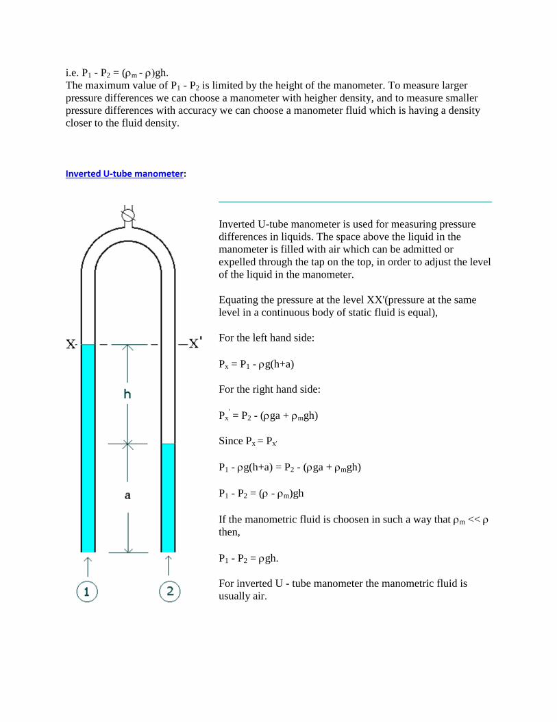
Flow of incompressible fluid in pipes:

Laminar flow

Pressure drop in turbulent flow

The head loss in turbulent flow in a circular pipe is given by,

hf = 2fLv2 / D = p /

where f is the friction factor, defined as

f = w / (v2/2)

where w is wall shear stress.

The value of friction factor f depends on the factors such as velocity (v) , pipe diameter (D) ,

density of fluid () , viscosity of fluid () and absolute roughness (k) of the pipe.

These variables are grouped as the dimensional numbers NRe and k/D

Where NRe = Dv/ = Reynolds number

and k/D is the relative roughness of the pipe.

Blasisus, in 1913 was, the first to propose an accurate empirical relation for the friction factor in

turbulent flow in smooth pipes, namely

f = 0.079 / NRe0.25

This expression yields results for head loss to + 5 percent for smooth pipes at Reynolds numbers

up to 100000.

For rough pipes, Nikuradse, in 1933, proved the validity of f dependence on the relative

roughness ratio k/D by investigating the head loss in a number of pipes which had been treated

internally with a coating of sand particles whose size could be varied.

Thus, the calculation of losses in turbulent pipe flow is dependent on the use of empirical results

and the most common reference source is the Moody chart, which is a logarithmic plot of f vs.

NRe for a range of k/D values. A typical Moody chart is presented as figure.

There are a number of distinct regions in the chart.

1. The straight line labeled 'laminar flow', representing f = 16/NRe, is a graphical

representation of the Poiseuille equation. The above equation plots as a straight line of

slope -1 on a log-log plot and is independent of the pipe surface roughness.

2. For values of k/D < 0.001 the rough pipe curves approach the Blasius smooth pipe curve.

Velocity Distribution for turbulent flow

No exact mathematical analysis of the conditions within a turbulent fluid has yet been developed,

though a number of semi-theoretical expressions for the shear stress at the walls of a pipe of

circular cross-section have been suggested.

The velocity at any point in the cross-section will be proportional to the one-seventh power of

the distance from the walls. This may be expressed as follows:

Where ux is the velocity at a distance y from the walls, uCL the velocity at the centerline of pipe,

and r the radius of the pipe.

This equation is referred to as the Prandtl one-seventh power law.

By using Prandtl one-seventh power law, the mean velocity of flow is found to be equal to 0.817

times the centerline velocity.

Surface roughness

Values of surface roughness for various materials:

Material Surface Roughness k, inch

Drawn tubing 0.00006

Commercial steel 0.0018

Galvanized iron 0.006

Cast iron 0.010

Wood stave 0.0072 - 0.036

Concrete 0.012 - 0.12

Riveted steel 0.036 - 0.36

Flow through non-circular pipes

For turbulent flow in a duct of non-circular cross-section, the hydraulic mean diameter may be

used in place of the pipe diameter and the formulae for circular pipes can then be applied without

introducing a large error. This method of approach is entirely empirical.

The hydraulic mean diameter DH is defined as four times the hydraulic mean radius rH.

Hydraulic mean radius is defined as the flow cross-sectional area divided by the wetted

perimeter: some examples are given. For circular pipe:

DH = 4(/4)D2 / (D) = D

For an annulus of outer dia Do and inner dia Di :

DH = 4 ( (Do2 /4) - (Di

2 /4) ) / ( (Do + Di) ) = (Do

2 - Di

2) / (Do + Di) = Do - Di

For a duct of rectangular cross-section Da by Db :

DH = 4 DaDb / ( 2(Da + Db) = 2DaDb / (Da + Db)

For a duct of square cross-section of size Da :

DH = 4 Da2 / (4Da) = Da

For laminar flow this method is not applicable, and exact expressions relating the pressure drop

to the velocity can be obtained for ducts of certain shapes only.

Flow through curved pipes

If the pipe is not straight, the velocity distribution over the section is altered and the direction of

flow of fluid is continuously changing. The frictional losses are therefore somewhat greater than

for a straight pipe of the same length. If the radius of the pipe divided by the radius of the bend is

less than about 0.002 however, the effects of the curvature are negligible.

It has been found that stable streamline flow persists at higher values of the Reynolds number in

coiled pipes. Thus for instance, when the ratio of the diameter of the pipe to the diameter of the

coil is 1 to 15, the transition occurs at a Reynolds number of about 8000.

Expansion losses

Contraction losses

Sudden Contraction

Losses for flow through fittings

Fitting Loss Coefficient, K

Gate valve (open to 75% shut) 0.25 - 25

Globe valve 10

Pump foot valve 1.5

Return bend 2.2

90o elbow 0.9

45o elbow 0.4

Large-radius 90o bend 0.6

Tee junction 1.8

Sharp pipe entry 0.5

Radiused pipe entry 0

Sharp pipe exit 0.5

Types of flow problems

The friction factor relates six parameters of the flow:

1. Pipe diameter

2. Average velocity

3. Fluid density

4. Fluid viscosity

5. Pipe roughness

6. The frictional losses per unit mass.

Therefore, given any five of these, we can use the friction-factor charts to find the sixth.

Most often, instead of being interested in the average velocity, we are interested in the

volumetric flow rate Q = (/4)D2V

The three most common types of problems are the following:

Type Given To find

1 D, k, , , Q hf

D, k, , , hf Q

k, , hf, Q D

Generally, type 1 can be solved directly, where as types 2 and 3 require simple trial and error.

Three fundamental problems which are commonly encountered in pipe-flow calculations:

Constants: , , g, L

1. Given D, and v or Q, compute the pressure drop. (pressure-drop problem)

2. Given D, delP, compute velocity or flow rate (flow-rate problem)

3. Given Q, delP, compute the diameter D of the pipe (sizing problem)

Compressible fluid flow:

Nozzles & diffusers

Unit –III

Closed channel flow measurement:

Venturi meter

In this meter the fluid is accelerated by its passage through a converging cone of angle

15-20o. The pressure difference between the upstream end if the cone and the throat is

measured and provides the signal for the rate of flow. The fluid is then retarded in a cone

of smaller angle (5-7o) in which large proportion of kinetic energy is converted back to

pressure energy. Because of the gradual reduction in the area there is no vena contracta

and the flow area is a minimum at the throat so that the coefficient of contraction is unity.

The attraction of this meter lies in its high energy recovery so that it may be used where

only a small pressure head is available, though its construction is expensive.

To make the pressure recovery large, the angle of downstream cone is small, so boundary

layer separation is prevented and friction minimized. Since separation does not occur in a

contracting cross section, the upstream cone can be made shorter than the downstream

cone with but little friction, and space and material are thereby conserved.

Although venturi meters can be applied to the measurement of gas, they are most

commonly used for liquids. The following treatment is limited to incompressible fluids.

The basic equation for the venturi meter is obtained by writing the Bernoulli equation for

incompressible fluids between the two sections a and b. Friction is neglected, the meter is

assumed to be horizontal.

If va and vb are the average upstream and downstream velocities, respectively, and is

the density of the fluid,

vb2 - va

2 = 2(pa - pb)/ 1

The continuity equation can be written as,

va = (Db/Da)2vb =

2vb 2

where Da = diameter of pipe

Db = diameter of throat of meter

= diameter ratio, Db/Da

If va is eliminated from equn.1 and 2, the result is

3

Equn.3 applies strictly to the frictionless flow of non-compressible fluids. To account for

the small friction loss between locations a and b, equn.3 is corrected by introducing an

empirical factor Cv. The coefficient Cv is determined experimentally. It is called the

venturi coefficient, velocity of approach not included. The effect of the approach velocity

va is accounted by the term 1/(1-4)0.5

. When Db is less than Da/4, the approach velocity

and the term can be neglected, since the resulting error is less than 0.2 percent.

For a well designed venturi, the constant Cv is about 0.98 for pipe diameters of 2 to 8 inch

and about 0.99 for larger sizes.

In a properly designed venturi meter, the permanent pressure loss is about 10% of the

venturi differential (pa - pb), and 90% of differential is recovered.

Volumetric flow rate:

The velocity through the venturi throat vb usually is not the quantity desired. The flow

rates of practical interest are the mass and volumetric flow rates through the meter.

Volumetric flow rate is calculated from,

Q = Abvb and mass flow rate from,

Mass flow rate = volumetric flow rate x density

The standard dimensions for the meter are:

Entrance cone angle (21) = 21+ 2o

Exit cone angle (22) = 5 to 15o

Throat length = one throat diameter

Orifice meter:

The venturi meter described earlier is a reliable flow measuring device. Furthermore, it causes

little pressure loss. For these reasons it is widely used, particularly for large-volume liquid and

gas flows. However this meter is relatively complex to construct and hence expensive. Especially

for small pipelines, its cost seems prohibitive, so simpler devices such as orifice meters are used.

The orifice meter consists of a flat orifice plate with a circular hole drilled in it. There is a

pressure tap upstream from the orifice plate and another just downstream. There are three

recognized methods of placing the taps. And the coefficient of the meter will depend upon the

position of taps.

Type of tap Distance of upstream tap

from face of orifice

Distance of downstream tap

from downstream face

Flange 1 inch 1 inch

Vena

contracta

1 pipe diameter (actual

inside)

0.3 to 0.8 pipe diameter,

depending on

Pipe 2.5 times nominal pipe

diameter 8 times nominal pipe diameter

The principle of the orifice meter is identical with that of the venturi meter. The reduction of

the cross section of the flowing stream in passing through the orifice increases the velocity head

at the expense of the pressure head, and the reduction in pressure between the taps is measured

by a manometer. Bernoulli's equation provides a basis for correlating the increase in velocity

head with the decrease in pressure head.

1

where = Db/Da = (Ab/Aa)0.5

One important complication appears in the orifice meter that is not found in the venturi. The area

of flow decreases from Aa at section 'a' to cross section of orifice opening (Ao) at the orifice and

then to Ab at the vena contracta. The area at the vena contracta can be conveniently related to the

area of the orifice by the coefficient of contraction Cc defined by the relation:

Cc = Ab / Ao

Therefore, vbAb = voAo , i.e., vo = vbCc

Inserting the value of Ab = CcAo in equn.1

using the coefficient of discharge Co (orifice coefficient) to take the account of frictional losses

in the meter and the parameter Cc, the flow rate (Q) through the pipe is obtained as,

Co varies considerably with changes in Ao/Aa ratio and Reynolds number. A orifice coefficient

(Co) of 0.61 may be taken for the standard meter for Reynolds numbers in excess of 104, though

the value changes noticeably at lower values of Reynolds number.

Orifice pressure recovery:

Permanent pressure loss depends on the value of ( = Do/Da). For a value of = 0.5, the lost

head is about 73% of the orifice differential.

Venturi - Orifice Comparison

In comparing the venturi meter with the orifice meter, both the cost of installation and the cost of

operation must be considered.

1. The orifice plate can easily be changed to accomodate widely different flow rates,

whereas the throat diameter of a venturi is fixed, so that its range of flow rates is

circumscribed by the practical limits of p.

2. The orifice meter has a large permanent loss of pressure because of the presence of

eddies on the downstream side of the orifice-plate; the shape of the venturi meter

prevents the formation os these eddies and greatly reduces the permanent loss.

3. The orifice is cheap and easy to install. The venturi meter is expensive, as it must be

carefully proportioned and fabricated. A home made orifice is often entirely satisfactory,

whereas a venturi meter is practically always purchased from an instrument dealer.

4. On the other hand, the head lost in the orifice for the same conditions as in the venturi is

many times greater. The power lost is proportionally greater, and, when an orifice is

inserted in a line carrying fluid continuously over long periods of time, the cost of the

power may be out of all proportion to the saving in first cost. Orifices are therefore best

used for testing purposes or other cases where the power lost is not a factor, as in steam

lines.

5. However, in spite of considerations of power loss, orifices are widely used, partly

because of their greater flexibility, because installing a new orifice plate with a different

opening is a simpler matter. The venturi meter can not be so altered. Venturi meters are

used only for permanent installations.

6. It should be noted that for a given pipe diameter and a given diameter of orifice opening

or venturi throat, the reading of the venturi meter for a given velocity is to the reading of

the orifice as (0.61/0.98)2, or 1:2.58.(i.e. orifice meter will show higher manometer

reading for a given velocity than venturi meter).

Pitot tube

The pitot tube is a device to measure the

local velocity along a streamline. The pitot

tube has two tubes: one is static tube(b),

and another is impact tube(a). The opening

of the impact tube is perpendicular to the

flow direction. The opening of the static

tube is parallel to the direction of flow. The

two legs are connected to the legs of a

manometer or equivalent device for

measuring small pressure differences. The

static tube measures the static pressure,

since there is no velocity component perpendicular to its opening. The impact tube measures

both the static pressure and impact pressure (due to kinetic energy). In terms of heads the impact

tube measures the static pressure head plus the velocity head.

The reading (hm) of the manometer will therefore measure the velocity head, and

v2/2g = Pressure head measured indicated by the pressure measuring device

i.e. v2/2 = p/

1

Pressure difference indicated by the manometer p is given by,

p = hm(m - )g

Pitot tube - A convenient setup:

It consists of two concentric tubes arranged

parallel to the direction of flow; the impact

pressure is measured on the open end of the inner

tube. The end of the outer concentric tube is

sealed and a series of orifices on the curved

surface give an accurate indication of the static

pressure. For the flow rate not to be appreciably

disturbed, the diameter of the instrument must

not exceed about one fifth of the diameter of the

pipe. An accurate measurement of the impact

pressure can be obtained using a tube of very

small diameter with its open end at right angles

to the direction of flow; hypodermic tubing is

convenient for this purpose.

The pitot tube measures the velocity of only a

filament of liquid, and hence it can be used for

exploring the velocity distribution across the pipe

cross-section. If, however, it is desired to

measure the total flow of fluid through the pipe,

the velocity must be measured at various distance

from the walls and the results integrated. The total flow rate can be calculated from a single

reading only of the velocity distribution across the cross-section is already known.

A perfect pitot tube should obey equn.1 exactly, but all actual instruments must be calibrated and

a correction factor applied.

Rotameter

In the variable head meters the area of constriction or orifice is constant and the drop in pressure

is dependent on the rate of flow. In the variable area meter, the drop in pressure is constant and

the flow rate is a function of the area of

constriction.

A typical meter of this kind, which is commonly

known as rotameter consists of a tapered glass

tube with the smallest diameter at the bottom. The

tube contains a freely moving float which rests on

a stop at the base of the tube. When the fluid is

flowing the float rises until its weight is balanced

by the upthrust of the fluid, the float reaches a

position of equilibrium, its position then indicating

the rate of flow. The flow rate can be read from

the adjacent scale, which is often etched on the

glass tube. The float is often stabilized by helical

grooves incised into it, which introduce rotation -

hence the name. Other shapes of the floats -

including spheres in the smaller instruments may

be employed.

The pressure drop across the float is equal to its

weight divided by its maximum cross-sectional area in the horizontal plane. The area for flow is

the annulus formed between the float and the wall of the tube.

This meter may thus be considered as an orifice meter with a variable aperture, and the formula

derived for orifice meter / venturi meter are applicable with

only minor changes.

Both in the orifice-type meter and in the rotameter the pressure

drop arises from the conversion of pressure energy to kinetic

energy (recall Bernoulli's equation) and from frictional losses

which are accounted for in the coefficient of discharge.

p/(g) = u22/(2g) - u1

2/(2g) 1

Continuity equation:

A1u1 = A2u2 2

Where A1 is the tube cross-section, and A2 is the cross-section of annulus (area between the tube

and float)

From equn.1 and 2,

3

The pressure drop over the float p, is given by:

p = Vf(f - )g / Af 4

where Vf is the volume of the float, f the density of the material of the float, and Af is the

maximum cross sectional area of the float in a horizontal plane.

Substituting for p from equn.4 in equn.3, and for the flow rate the equation is arrived as

The coefficient CD depends on the shape of the float and the Reynolds number (based on the

velocity in the annulus and the mean hydraulic diameter of the annulus) for the annular space of

area A2.

In general, floats which give the most nearly constant

coefficient are of such a shape that they set up eddy

currents and give low values of CD.

The constant coefficient for the float C arises from

turbulence promotion, and for this reason the

coefficient is also substantially independent of the fluid

viscosity. The meter can be made relatively insensitive

to changes in the density of the fluid by the selection of

the density of float, f. If the density of the float is

twice that of the fluid, then the position of the float for

a given float is independent of the fluid density.

Because of variable-area flowmeter relies on gravity, it

must be installed vertically (with the flowtube

perpendicular to the floor).

The range of a meter can be increased by the use of floats of different densities. For high

pressure work the glass tube is replaced by a metal tube. When a metal tube is used or when the

liquid is very dark or dirty an external indicator is required.

The advantage of rotameters are direct visual readings, wide range, nearly linear scale, and

constant (and small) head loss. It requires no straight pipe runs before and after the meter.

Open channel flow measurement:

Elementary theory of weirs and notches

Elementary theory of Notches and Weirs:

A notch is an opening in the side of a measuring tank or reservoir extending above the free

surface. A weir is a notch on a large scale, used, for example, to measure the flow of a river, and

may be sharp edged or have a substantial breadth in the direction of flow.

The method of determining the theoretical flow through a notch is the same as that adopted for a

large orifice.

For a notch of any shape shown in figure, consider a horizontal strip of width b at a depth h

below the free surface and height h.

Area of strip = bh.

Velocity through strip = (2gh)

Discharge through strip, Q = Area x velocity = bh (2gh).

Integrating from h = 0 at the free surface to h = H at the bottom of the notch,

Total theoretical discharge(Q),

1

Before the integration of equn.1 can be carried out, b must be expressed in terms of h.

Rectangular Notch:

For a rectangular notch, put b = constant = B in equn.1 giving,

2

V-Notch:

For a V-notch with an included angle put b = 2(H-h)tan(/2) in equn.1, giving

i.e.,

3

Inspection of equns.2 and 3 suggests that, by choosing a suitable shape for the sides of the notch,

any desired relationship between Q and H could be achieved.

As in the case of orifice, the actual discharge through a notch or weir can be found by

multiplying the theoretical discharge by a coefficient of discharge to allow for energy losses and

the contraction of the cross-section of the stream at the bottom and sides.

In the forgoing theory, it has been assumed that the velocity of the liquid approaching the notch

is very small so that its kinetic energy can be neglected; it can also be assumed that the velocity

through any horizontal element across the notch will depend only on its depth below the free

surface. This is a satisfactory assumption for flow over a notch or weir in the side of a large

reservoir, but, is the notch or weir is placed at the end of a narrow channel, the velocity of

approach to the weir will be substantial and the head h producing flow will be increased by the

kinetic energy of the approaching liquid to a value

x = h + v12/(2g),

where v1 is the mean velocity of the liquid in the approach channel. Note that the value of v1 is

obtained by dividing the discharge by the full cross sectional area of the channel itself, not that of

the notch. As a result, the discharge through the strip will be

Q = bh (2gx).

Coefficient of Discharge for Rectangular Weir:

Coefficient of discharge for rectangular weir given by Rehbock is,

Where P is the height of weir crest in meter.

H is the head over crest in meter.

The above equation is valid for P from 0.1 to 1.0 m and H from 0.024 to 0.6 m.

Suppressed weirs:

When the length of crest of the weir is same as the width of the channel, the weir is said to be

suppressed weir. Thus in this case, the effects of sides of the weir is eliminated or suppressed.

Thus for suppressed weirs, length of weir crest = width of channel.

Contracted weirs:

When the crest length of a rectangular weir is less than the width of the channel, there will be

lateral contraction.

Flow rate (Q) for contracted rectangular weirs is estimated from,

Where n is the number of contractions.

n = 0 if the notch is full width of the channel;

n = 1 if the notch is narrower than the channel but is arranged with one edge coincident with the

edge of the channel;

n = 2 if the notch is narrower than the channel and is situated symmetrically.

Submerged weir:

When the water on the downstream side of a weir rises above the level of the crest, the weir is

said to be a submerged weir.

The flow over the submerged weir may be considered by dividing the flow into two portions:

1. Flow over the upper part of the line AB may be considered as weir flow (H1-H2). (flow

rate Q1)

2. Flow through the remaining depth H2 may be considered as discharge through a

submerged orifice. (flow rate Q2)

Q1 = (2/3)Cd1B(H1-H2)3/2

(2g)

Q2 = Cd2BH2 (2g(H1-H2))

Total flow rate Q = Q1 + Q2

Trapezoidal Notch:

The equation for flow through trapezoidal notch is obtained from the equations for rectangular

and V-notches.

Rectangular notch

Elementary theory of Notches and Weirs:

A notch is an opening in the side of a measuring tank or reservoir extending above the free

surface. A weir is a notch on a large scale, used, for example, to measure the flow of a river, and

may be sharp edged or have a substantial breadth in the direction of flow.

The method of determining the theoretical flow through a notch is the same as that adopted for a

large orifice.

For a notch of any shape shown in figure, consider a horizontal strip of width b at a depth h

below the free surface and height h.

Area of strip = bh.

Velocity through strip = (2gh)

Discharge through strip, Q = Area x velocity = bh (2gh).

Integrating from h = 0 at the free surface to h = H at the bottom of the notch,

Total theoretical discharge(Q),

1

Before the integration of equn.1 can be carried out, b must be expressed in terms of h.

Rectangular Notch:

For a rectangular notch, put b = constant = B in equn.1 giving,

2

V-Notch:

For a V-notch with an included angle put b = 2(H-h)tan(/2) in equn.1, giving

i.e.,

3

Inspection of equns.2 and 3 suggests that, by choosing a suitable shape for the sides of the notch,

any desired relationship between Q and H could be achieved.

As in the case of orifice, the actual discharge through a notch or weir can be found by

multiplying the theoretical discharge by a coefficient of discharge to allow for energy losses and

the contraction of the cross-section of the stream at the bottom and sides.

In the forgoing theory, it has been assumed that the velocity of the liquid approaching the notch

is very small so that its kinetic energy can be neglected; it can also be assumed that the velocity

through any horizontal element across the notch will depend only on its depth below the free

surface. This is a satisfactory assumption for flow over a notch or weir in the side of a large

reservoir, but, is the notch or weir is placed at the end of a narrow channel, the velocity of

approach to the weir will be substantial and the head h producing flow will be increased by the

kinetic energy of the approaching liquid to a value

x = h + v12/(2g),

where v1 is the mean velocity of the liquid in the approach channel. Note that the value of v1 is

obtained by dividing the discharge by the full cross sectional area of the channel itself, not that of

the notch. As a result, the discharge through the strip will be

Q = bh (2gx).

Coefficient of Discharge for Rectangular Weir:

Coefficient of discharge for rectangular weir given by Rehbock is,

Where P is the height of weir crest in meter.

H is the head over crest in meter.

The above equation is valid for P from 0.1 to 1.0 m and H from 0.024 to 0.6 m.

Suppressed weirs:

When the length of crest of the weir is same as the width of the channel, the weir is said to be

suppressed weir. Thus in this case, the effects of sides of the weir is eliminated or suppressed.

Thus for suppressed weirs, length of weir crest = width of channel.

Contracted weirs:

When the crest length of a rectangular weir is less than the width of the channel, there will be

lateral contraction.

Flow rate (Q) for contracted rectangular weirs is estimated from,

Where n is the number of contractions.

n = 0 if the notch is full width of the channel;

n = 1 if the notch is narrower than the channel but is arranged with one edge coincident with the

edge of the channel;

n = 2 if the notch is narrower than the channel and is situated symmetrically.

Submerged weir:

When the water on the downstream side of a weir rises above the level of the crest, the weir is

said to be a submerged weir.

The flow over the submerged weir may be considered by dividing the flow into two portions:

1. Flow over the upper part of the line AB may be considered as weir flow (H1-H2). (flow

rate Q1)

2. Flow through the remaining depth H2 may be considered as discharge through a

submerged orifice. (flow rate Q2)

Q1 = (2/3)Cd1B(H1-H2)3/2

(2g)

Q2 = Cd2BH2 (2g(H1-H2))

Total flow rate Q = Q1 + Q2

Trapezoidal Notch:

The equation for flow through trapezoidal notch is obtained from the equations for rectangular

and V-notches.

V-notch

Elementary theory of Notches and Weirs:

A notch is an opening in the side of a measuring tank or reservoir extending above the free

surface. A weir is a notch on a large scale, used, for example, to measure the flow of a river, and

may be sharp edged or have a substantial breadth in the direction of flow.

The method of determining the theoretical flow through a notch is the same as that adopted for a

large orifice.

For a notch of any shape shown in figure, consider a horizontal strip of width b at a depth h

below the free surface and height h.

Area of strip = bh.

Velocity through strip = (2gh)

Discharge through strip, Q = Area x velocity = bh (2gh).

Integrating from h = 0 at the free surface to h = H at the bottom of the notch,

Total theoretical discharge(Q),

1

Before the integration of equn.1 can be carried out, b must be expressed in terms of h.

Rectangular Notch:

For a rectangular notch, put b = constant = B in equn.1 giving,

2

V-Notch:

For a V-notch with an included angle put b = 2(H-h)tan(/2) in equn.1, giving

i.e.,

3

Inspection of equns.2 and 3 suggests that, by choosing a suitable shape for the sides of the notch,

any desired relationship between Q and H could be achieved.

As in the case of orifice, the actual discharge through a notch or weir can be found by

multiplying the theoretical discharge by a coefficient of discharge to allow for energy losses and

the contraction of the cross-section of the stream at the bottom and sides.

In the forgoing theory, it has been assumed that the velocity of the liquid approaching the notch

is very small so that its kinetic energy can be neglected; it can also be assumed that the velocity

through any horizontal element across the notch will depend only on its depth below the free

surface. This is a satisfactory assumption for flow over a notch or weir in the side of a large

reservoir, but, is the notch or weir is placed at the end of a narrow channel, the velocity of

approach to the weir will be substantial and the head h producing flow will be increased by the

kinetic energy of the approaching liquid to a value

x = h + v12/(2g),

where v1 is the mean velocity of the liquid in the approach channel. Note that the value of v1 is

obtained by dividing the discharge by the full cross sectional area of the channel itself, not that of

the notch. As a result, the discharge through the strip will be

Q = bh (2gx).

Coefficient of Discharge for Rectangular Weir:

Coefficient of discharge for rectangular weir given by Rehbock is,

Where P is the height of weir crest in meter.

H is the head over crest in meter.

The above equation is valid for P from 0.1 to 1.0 m and H from 0.024 to 0.6 m.

Suppressed weirs:

When the length of crest of the weir is same as the width of the channel, the weir is said to be

suppressed weir. Thus in this case, the effects of sides of the weir is eliminated or suppressed.

Thus for suppressed weirs, length of weir crest = width of channel.

Contracted weirs:

When the crest length of a rectangular weir is less than the width of the channel, there will be

lateral contraction.

Flow rate (Q) for contracted rectangular weirs is estimated from,

Where n is the number of contractions.

n = 0 if the notch is full width of the channel;

n = 1 if the notch is narrower than the channel but is arranged with one edge coincident with the

edge of the channel;

n = 2 if the notch is narrower than the channel and is situated symmetrically.

Submerged weir:

When the water on the downstream side of a weir rises above the level of the crest, the weir is

said to be a submerged weir.

The flow over the submerged weir may be considered by dividing the flow into two portions:

1. Flow over the upper part of the line AB may be considered as weir flow (H1-H2). (flow

rate Q1)

2. Flow through the remaining depth H2 may be considered as discharge through a

submerged orifice. (flow rate Q2)

Q1 = (2/3)Cd1B(H1-H2)3/2

(2g)

Q2 = Cd2BH2 (2g(H1-H2))

Total flow rate Q = Q1 + Q2

Trapezoidal Notch:

The equation for flow through trapezoidal notch is obtained from the equations for rectangular

and V-notches.

Suppressed and contracted weirs

Elementary theory of Notches and Weirs:

A notch is an opening in the side of a measuring tank or reservoir extending above the free

surface. A weir is a notch on a large scale, used, for example, to measure the flow of a river, and

may be sharp edged or have a substantial breadth in the direction of flow.

The method of determining the theoretical flow through a notch is the same as that adopted for a

large orifice.

For a notch of any shape shown in figure, consider a horizontal strip of width b at a depth h

below the free surface and height h.

Area of strip = bh.

Velocity through strip = (2gh)

Discharge through strip, Q = Area x velocity = bh (2gh).

Integrating from h = 0 at the free surface to h = H at the bottom of the notch,

Total theoretical discharge(Q),

1

Before the integration of equn.1 can be carried out, b must be expressed in terms of h.

Rectangular Notch:

For a rectangular notch, put b = constant = B in equn.1 giving,

2

V-Notch:

For a V-notch with an included angle put b = 2(H-h)tan(/2) in equn.1, giving

i.e.,

3

Inspection of equns.2 and 3 suggests that, by choosing a suitable shape for the sides of the notch,

any desired relationship between Q and H could be achieved.

As in the case of orifice, the actual discharge through a notch or weir can be found by

multiplying the theoretical discharge by a coefficient of discharge to allow for energy losses and

the contraction of the cross-section of the stream at the bottom and sides.

In the forgoing theory, it has been assumed that the velocity of the liquid approaching the notch

is very small so that its kinetic energy can be neglected; it can also be assumed that the velocity

through any horizontal element across the notch will depend only on its depth below the free

surface. This is a satisfactory assumption for flow over a notch or weir in the side of a large

reservoir, but, is the notch or weir is placed at the end of a narrow channel, the velocity of

approach to the weir will be substantial and the head h producing flow will be increased by the

kinetic energy of the approaching liquid to a value

x = h + v12/(2g),

where v1 is the mean velocity of the liquid in the approach channel. Note that the value of v1 is

obtained by dividing the discharge by the full cross sectional area of the channel itself, not that of

the notch. As a result, the discharge through the strip will be

Q = bh (2gx).

Coefficient of Discharge for Rectangular Weir:

Coefficient of discharge for rectangular weir given by Rehbock is,

Where P is the height of weir crest in meter.

H is the head over crest in meter.

The above equation is valid for P from 0.1 to 1.0 m and H from 0.024 to 0.6 m.

Suppressed weirs:

When the length of crest of the weir is same as the width of the channel, the weir is said to be

suppressed weir. Thus in this case, the effects of sides of the weir is eliminated or suppressed.

Thus for suppressed weirs, length of weir crest = width of channel.

Contracted weirs:

When the crest length of a rectangular weir is less than the width of the channel, there will be

lateral contraction.

Flow rate (Q) for contracted rectangular weirs is estimated from,

Where n is the number of contractions.

n = 0 if the notch is full width of the channel;

n = 1 if the notch is narrower than the channel but is arranged with one edge coincident with the

edge of the channel;

n = 2 if the notch is narrower than the channel and is situated symmetrically.

Submerged weir:

When the water on the downstream side of a weir rises above the level of the crest, the weir is

said to be a submerged weir.

The flow over the submerged weir may be considered by dividing the flow into two portions:

1. Flow over the upper part of the line AB may be considered as weir flow (H1-H2). (flow

rate Q1)

2. Flow through the remaining depth H2 may be considered as discharge through a

submerged orifice. (flow rate Q2)

Q1 = (2/3)Cd1B(H1-H2)3/2

(2g)

Q2 = Cd2BH2 (2g(H1-H2))

Total flow rate Q = Q1 + Q2

Trapezoidal Notch:

The equation for flow through trapezoidal notch is obtained from the equations for rectangular

and V-notches.

Submerged weirs

Elementary theory of Notches and Weirs:

A notch is an opening in the side of a measuring tank or reservoir extending above the free

surface. A weir is a notch on a large scale, used, for example, to measure the flow of a river, and

may be sharp edged or have a substantial breadth in the direction of flow.

The method of determining the theoretical flow through a notch is the same as that adopted for a

large orifice.

For a notch of any shape shown in figure, consider a horizontal strip of width b at a depth h

below the free surface and height h.

Area of strip = bh.

Velocity through strip = (2gh)

Discharge through strip, Q = Area x velocity = bh (2gh).

Integrating from h = 0 at the free surface to h = H at the bottom of the notch,

Total theoretical discharge(Q),

1

Before the integration of equn.1 can be carried out, b must be expressed in terms of h.

Rectangular Notch:

For a rectangular notch, put b = constant = B in equn.1 giving,

2

V-Notch:

For a V-notch with an included angle put b = 2(H-h)tan(/2) in equn.1, giving

i.e.,

3

Inspection of equns.2 and 3 suggests that, by choosing a suitable shape for the sides of the notch,

any desired relationship between Q and H could be achieved.

As in the case of orifice, the actual discharge through a notch or weir can be found by

multiplying the theoretical discharge by a coefficient of discharge to allow for energy losses and

the contraction of the cross-section of the stream at the bottom and sides.

In the forgoing theory, it has been assumed that the velocity of the liquid approaching the notch

is very small so that its kinetic energy can be neglected; it can also be assumed that the velocity

through any horizontal element across the notch will depend only on its depth below the free

surface. This is a satisfactory assumption for flow over a notch or weir in the side of a large

reservoir, but, is the notch or weir is placed at the end of a narrow channel, the velocity of

approach to the weir will be substantial and the head h producing flow will be increased by the

kinetic energy of the approaching liquid to a value

x = h + v12/(2g),

where v1 is the mean velocity of the liquid in the approach channel. Note that the value of v1 is

obtained by dividing the discharge by the full cross sectional area of the channel itself, not that of

the notch. As a result, the discharge through the strip will be

Q = bh (2gx).

Coefficient of Discharge for Rectangular Weir:

Coefficient of discharge for rectangular weir given by Rehbock is,

Where P is the height of weir crest in meter.

H is the head over crest in meter.

The above equation is valid for P from 0.1 to 1.0 m and H from 0.024 to 0.6 m.

Suppressed weirs:

When the length of crest of the weir is same as the width of the channel, the weir is said to be

suppressed weir. Thus in this case, the effects of sides of the weir is eliminated or suppressed.

Thus for suppressed weirs, length of weir crest = width of channel.

Contracted weirs:

When the crest length of a rectangular weir is less than the width of the channel, there will be

lateral contraction.

Flow rate (Q) for contracted rectangular weirs is estimated from,

Where n is the number of contractions.

n = 0 if the notch is full width of the channel;

n = 1 if the notch is narrower than the channel but is arranged with one edge coincident with the

edge of the channel;

n = 2 if the notch is narrower than the channel and is situated symmetrically.

Submerged weir:

When the water on the downstream side of a weir rises above the level of the crest, the weir is

said to be a submerged weir.

The flow over the submerged weir may be considered by dividing the flow into two portions:

1. Flow over the upper part of the line AB may be considered as weir flow (H1-H2). (flow

rate Q1)

2. Flow through the remaining depth H2 may be considered as discharge through a

submerged orifice. (flow rate Q2)

Q1 = (2/3)Cd1B(H1-H2)3/2

(2g)

Q2 = Cd2BH2 (2g(H1-H2))

Total flow rate Q = Q1 + Q2

Trapezoidal Notch:

The equation for flow through trapezoidal notch is obtained from the equations for rectangular

and V-notches.

Trapezoidal notch

Elementary theory of Notches and Weirs:

A notch is an opening in the side of a measuring tank or reservoir extending above the free

surface. A weir is a notch on a large scale, used, for example, to measure the flow of a river, and

may be sharp edged or have a substantial breadth in the direction of flow.

The method of determining the theoretical flow through a notch is the same as that adopted for a

large orifice.

For a notch of any shape shown in figure, consider a horizontal strip of width b at a depth h

below the free surface and height h.

Area of strip = bh.

Velocity through strip = (2gh)

Discharge through strip, Q = Area x velocity = bh (2gh).

Integrating from h = 0 at the free surface to h = H at the bottom of the notch,

Total theoretical discharge(Q),

1

Before the integration of equn.1 can be carried out, b must be expressed in terms of h.

Rectangular Notch:

For a rectangular notch, put b = constant = B in equn.1 giving,

2

V-Notch:

For a V-notch with an included angle put b = 2(H-h)tan(/2) in equn.1, giving

i.e.,

3

Inspection of equns.2 and 3 suggests that, by choosing a suitable shape for the sides of the notch,

any desired relationship between Q and H could be achieved.

As in the case of orifice, the actual discharge through a notch or weir can be found by

multiplying the theoretical discharge by a coefficient of discharge to allow for energy losses and

the contraction of the cross-section of the stream at the bottom and sides.

In the forgoing theory, it has been assumed that the velocity of the liquid approaching the notch

is very small so that its kinetic energy can be neglected; it can also be assumed that the velocity

through any horizontal element across the notch will depend only on its depth below the free

surface. This is a satisfactory assumption for flow over a notch or weir in the side of a large

reservoir, but, is the notch or weir is placed at the end of a narrow channel, the velocity of

approach to the weir will be substantial and the head h producing flow will be increased by the

kinetic energy of the approaching liquid to a value

x = h + v12/(2g),

where v1 is the mean velocity of the liquid in the approach channel. Note that the value of v1 is

obtained by dividing the discharge by the full cross sectional area of the channel itself, not that of

the notch. As a result, the discharge through the strip will be

Q = bh (2gx).

Coefficient of Discharge for Rectangular Weir:

Coefficient of discharge for rectangular weir given by Rehbock is,

Where P is the height of weir crest in meter.

H is the head over crest in meter.

The above equation is valid for P from 0.1 to 1.0 m and H from 0.024 to 0.6 m.

Suppressed weirs:

When the length of crest of the weir is same as the width of the channel, the weir is said to be

suppressed weir. Thus in this case, the effects of sides of the weir is eliminated or suppressed.

Thus for suppressed weirs, length of weir crest = width of channel.

Contracted weirs:

When the crest length of a rectangular weir is less than the width of the channel, there will be

lateral contraction.

Flow rate (Q) for contracted rectangular weirs is estimated from,

Where n is the number of contractions.

n = 0 if the notch is full width of the channel;

n = 1 if the notch is narrower than the channel but is arranged with one edge coincident with the

edge of the channel;

n = 2 if the notch is narrower than the channel and is situated symmetrically.

Submerged weir:

When the water on the downstream side of a weir rises above the level of the crest, the weir is

said to be a submerged weir.

The flow over the submerged weir may be considered by dividing the flow into two portions:

1. Flow over the upper part of the line AB may be considered as weir flow (H1-H2). (flow

rate Q1)

2. Flow through the remaining depth H2 may be considered as discharge through a

submerged orifice. (flow rate Q2)

Q1 = (2/3)Cd1B(H1-H2)3/2

(2g)

Q2 = Cd2BH2 (2g(H1-H2))

Total flow rate Q = Q1 + Q2

Trapezoidal Notch:

The equation for flow through trapezoidal notch is obtained from the equations for rectangular

and V-notches.

Unit –IV

Flow past immersed bodies:

Force in the direction of flow exerted by the fluid on the solid is called drag.

Figure shows a stationary smooth sphere of diameter DP situated in a stream, whose velocity far

away from the sphere is u to the right. Except at very low velocities, when the flow is entirely

laminar, the wake immediately downstream from the sphere is unstable, and turbulent vortices

will constantly be shed from various locations round the sphere. Because of turbulence, the

pressure on the downstream side of the sphere will never fully recovered to that on the upstream

side, and there will be a form drag to the right of the sphere. (For purely laminar flow, the

pressure recovery is complete, and the form drag is zero.)

In addition, because of the velocity gradients that exist near the sphere, there will also be a net

viscous drag (also called as wall drag) to the right (In potential flow there is no wall drag). The

sum of these two effects is known as the (total) drag force, FD. A similar drag occurs for spheres

and other objects moving through an otherwise stationary fluid - it is the relative velocity that

counts.

Form drag can be minimized by forcing separations toward the rear of the body. This is

accomplished by stream lining. (see figure)

The experimental results of the drag on a smooth sphere may be correlated in terms of two

dimensionless groups - the drag coefficient CD and particles Reynolds number NReP:

NReP = u DP/

In which AP = DP2/4 is the projected area of the sphere in the direction of motion, and and

are the properties of the fluid.

There are at least three distinct regions, for flow around a sphere.

1. For NReP less than 1 (laminar), CD vs. NReP is a straight line, and is given by the relation

CD = 24/NReP (given by Stoke's law, FD = 3 u DP)

2. 1 < NReP < 1000 , CD = 18 NReP-0.6

(transition)

3. 1000 < NReP < 2 x 105 , CD = 0.44 (turbulent)

For cylinders and disks, for NReP up to 1, CD = 24/NRe and in other regimes CD varies with NReP

in the manner as shown in figure. Here the flow orientation is much important. Drag coefficients

varies with orientation of solid to the flow direction.

In all these curves the transition from laminar to turbulent flow is more gradual than that for pipe

flow (f vs. NRe curve).

Friction in flow through bed of solids:

Consider a porous medium consisting of sand or some porous rock or glass beads or cotton cloth

contained in a pipe. At any one cross section perpendicular to the flow, the average velocity may

be based on the entire cross sectional area of pipe, in which case it is called the superficial

velocity Vs

Or it may be based on the area actually open to the flowing fluid, in which case it is called the

interstitial velocity VI

Where is the porosity or void fraction.

Previously it was indicated that for non-circular ducts, the friction factor plot could be used if we

replaced the diameter in both the friction factor and the Reynolds number with 4 times the

hydraulic radius (rH)

The hydraulic radius (rH) is the cross sectional area perpendicular to flow divided by the wetted

perimeter. For a uniform duct this is a constant. For a packed bed it varies from point to point.

But if we multiply both the cross sectional area and the perimeter by the length of the bed, it

becomes,

rH for porous medium = volume open to flow / total wetted surface

i.e.

But,

Therefore,

i.e.

i.e.

hf = p / = 2fLVI2 / De

substituting for VI in terms of VS

i.e. VI = VS /

NRe = De VI /

Substituting for De and VI

As in the case of flow in pipes, there are several different friction factors in common usage for

flowing in porous media, all differing by a constant.

i.e. fPM = 3f

and NRePM = 3NRe / 2

For laminar flow, f = 16 / NRe

Therefore,

fPM / 3 = 16 / (2NRePM / 3)

fPM = 72 / NRePM

There is one obvious error in this derivation, namely the tacit assumption that the flow is in the x

direction.

Actually, the flow is zigzag; it must pass around one particle and then through another. If we

assume that this zigzag proceeds with an average angle 45o to the x axis, then the actual flow

path is 2 times as long as the flow path, and the actual interstitial velocity is 2 times the

interstitial velocity used in the above equation. If we make these changes, we conclude that to

agree with the friction factor plot, laminar flow in a porous medium made of uniformly sized

spheres should be described by fPM = 144 / NRePM

Experimental data indicate that the constant is about 150, so that for laminar flow we find

experimentally,

fPM = 150 / NRePM

i.e.

This equation is called as Blake-Kozeny equation or as Kozeny-Carman equation. It is valid for

NRePM less than about 10.

Turbulent flow:

fPM = 1.75 (experimental value)

Therefore,

This is the Burke-Plummer equation, valid for NRePM greater than 1000

Since there is a smooth transition from all-laminar to all-turbulent flow, Ergun showed that if we

add the friction factor term,

fPM = 1.75 + 150 / NRePM

the transition regions data are predicted reasonably well.

i.e.

This is the Ergun's equation.

For non-spherical particles instead of diameter an equivalent diameter is defined.

The equivalent diameter of a non-spherical particle is defined as a sphere having the same

volume as the particle. Sphericity is the ratio of surface area of this sphere to the actual surface

area of particle.

The formula for sphericity is reduced to

Sphericity (s) = 6vp/ (DpSp)

Where vp is the volume of particle, Dp is the characteristic dimension of particle, and Sp is the

surface area of particle.

For non-spherical particle Ergun equation is given by,

Packed Towers:

Packed towers are finding applications in adsorption, absorption, ion-exchange, distillation,

humdification, catalytic reactions, regenerative heaters etc.,

The packing is to provide a good contact between the contacting phases.

Based on the method of packing, packings are classified as (a) Random packings and (b) Stacked

packings

There are a variety of materials that are being used as random packings. The packings are made

with clay, porcelain, plastics or metals. The following table gives the different packing materials

and their approximate void fraction.

Packing Void fraction

Berl saddle 0.6 - 0.7

Intalox saddle 0.7 - 0.8

Rasching ring 0.6 - 0.7

Pall ring 0.9 - 0.95

Principal requirements of a tower packing are:

1. It must be chemically inert to the fluids in the tower.

2. It must be strong without excessive weight.

3. It must contain adequate passages for the contacting streams without excessive pressure

drop.

4. It must provide good contact between the contacting phases.

5. It should be reasonable in cost.

Two-phase counter current flow of liquid and gas:

Normally, the denser fluid (e.g. water) runs down the surface of the packings by gravity, while

the less dense fluid flows upward because it is introduced at the bottom of the tower at a higher

pressure than it is with drawn from the top.

Fluidization:

Minimum fluidizing velocity

Fluidization refers to those gas-solids and liquid-solids system in which the solid phase is

subjected to behave more or less like a fluid by the upwelling current of gas or liquid stream

moving through the bed of solid particles.

Fluidized bed combustion and catalytic cracking of heavy crude-oil fractions of petroleum are

the two good examples of fluidization.

Fluidization starts at a point when the bed pressure drop exactly balances the net downward

forces (gravity minus buoyancy forces) on the bed packing, so

p/L = (1-)(s - )g 1

2

substituting for p/L from Ergun's equation,

In most industrial applications involving fluidized beds, the particle diameter is small, and VS

also small. In these cases, the second term of the above equation is negligible compared to the

first, so that

3

For a given bed the above equation can be used for both the unexpanded and the expanded state.

Pressure Drop Behavior of Fluidized beds:

As VS increases, may increase and hold p constant (L will also increase but its effect is much

less than the effect of change in See all the above equations). Thus the experimental result for

such a test is shown in figure.

For velocities less than the minimum

fluidization velocity Vmf, the bed behaves

as a packed bed. However as the velocity is

increased past Vmf, not only does the bed

expand (L increases), but also the particles

move apart, and also increases to keep the

p constant.

As the velocity is further increased, the bed

become more and more expanded, and the

solid content becomes more and more

dilute. Finally, the velocity becomes as

large as terminal settling velocity Vt of the

individual particles, so the particles are

blown out of the system. Thus the velocity

range for which a fluidized bed can exist is

from Vmf (can be calculated from equn.2) to

Vt.

Types of fluidization

The equations derived for minimum fluidization velocity apply to liquids as well as gases, but

beyond the minimum fluidization velocity Vmf, the appearance of beds with liquids or gases is

quite different.

When fluidizing sand with water, the particles move further apart and their motion becomes

more vigorous as the velocity is increased, but the bed density at a given velocity is same in all

sections of the bed. This is called particulate fluidization and is characterized by a large but

uniform expansion of the bed at high velocities.

Beds of solids fluidized with air usually exhibit what is called aggregative or bubbling

fluidization. At superficial velocities much greater than Vmf most of the gas passes through the

bed as bubbles or voids which are almost free of solids, and only a small fraction of the gas flows

in the channels between the particles.

Advantages and Disadvantages of fluidization:

The chief advantage of fluidization are that the solid is vigorously agitated by the fluid passing

through the bed, and the mixing of the solid ensures that there are practically no temperature

gradients in the bed even with quite exothermic or endothermic reactions.

Disadvantages:

1. The main disadvantage of gas-solid fluidization is the uneven contacting of gas and solid.

2. Erosion of vessel internals

3. Attrition of solids. Because of attrition, the size of the solid particles is getting reduced

and possibility for entrapment of solid particles with the fluid are more.

Pressure Drop in Fluidized bed

Fluidization refers to those gas-solids and liquid-solids system in which the solid phase is

subjected to behave more or less like a fluid by the upwelling current of gas or liquid stream

moving through the bed of solid particles.

Fluidized bed combustion and catalytic cracking of heavy crude-oil fractions of petroleum are

the two good examples of fluidization.

Fluidization starts at a point when the bed pressure drop exactly balances the net downward

forces (gravity minus buoyancy forces) on the bed packing, so

p/L = (1-)(s - )g 1

2

substituting for p/L from Ergun's equation,

In most industrial applications involving fluidized beds, the particle diameter is small, and VS

also small. In these cases, the second term of the above equation is negligible compared to the

first, so that

3

For a given bed the above equation can be used for both the unexpanded and the expanded state.

Pressure Drop Behavior of Fluidized beds:

As VS increases, may increase and hold p constant (L will also increase but its effect is much

less than the effect of change in See all the above equations). Thus the experimental result for

such a test is shown in figure.

For velocities less than the minimum

fluidization velocity Vmf, the bed behaves

as a packed bed. However as the velocity is

increased past Vmf, not only does the bed

expand (L increases), but also the particles

move apart, and also increases to keep the

p constant.

As the velocity is further increased, the bed

become more and more expanded, and the

solid content becomes more and more

dilute. Finally, the velocity becomes as

large as terminal settling velocity Vt of the

individual particles, so the particles are

blown out of the system. Thus the velocity

range for which a fluidized bed can exist is

from Vmf (can be calculated from equn.2) to

Vt.

Types of fluidization

The equations derived for minimum fluidization velocity apply to liquids as well as gases, but

beyond the minimum fluidization velocity Vmf, the appearance of beds with liquids or gases is

quite different.

When fluidizing sand with water, the particles move further apart and their motion becomes

more vigorous as the velocity is increased, but the bed density at a given velocity is same in all

sections of the bed. This is called particulate fluidization and is characterized by a large but

uniform expansion of the bed at high velocities.

Beds of solids fluidized with air usually exhibit what is called aggregative or bubbling

fluidization. At superficial velocities much greater than Vmf most of the gas passes through the

bed as bubbles or voids which are almost free of solids, and only a small fraction of the gas flows

in the channels between the particles.

Advantages and Disadvantages of fluidization:

The chief advantage of fluidization are that the solid is vigorously agitated by the fluid passing

through the bed, and the mixing of the solid ensures that there are practically no temperature

gradients in the bed even with quite exothermic or endothermic reactions.

Disadvantages:

1. The main disadvantage of gas-solid fluidization is the uneven contacting of gas and solid.

2. Erosion of vessel internals

3. Attrition of solids. Because of attrition, the size of the solid particles is getting reduced

and possibility for entrapment of solid particles with the fluid are more.

Fluidization Types

Fluidization refers to those gas-solids and liquid-solids system in which the solid phase is

subjected to behave more or less like a fluid by the upwelling current of gas or liquid stream

moving through the bed of solid particles.

Fluidized bed combustion and catalytic cracking of heavy crude-oil fractions of petroleum are

the two good examples of fluidization.

Fluidization starts at a point when the bed pressure drop exactly balances the net downward

forces (gravity minus buoyancy forces) on the bed packing, so

p/L = (1-)(s - )g 1

2

substituting for p/L from Ergun's equation,

In most industrial applications involving fluidized beds, the particle diameter is small, and VS

also small. In these cases, the second term of the above equation is negligible compared to the

first, so that

3

For a given bed the above equation can be used for both the unexpanded and the expanded state.

Pressure Drop Behavior of Fluidized beds:

As VS increases, may increase and hold p constant (L will also increase but its effect is much

less than the effect of change in See all the above equations). Thus the experimental result for

such a test is shown in figure.

For velocities less than the minimum

fluidization velocity Vmf, the bed behaves

as a packed bed. However as the velocity is

increased past Vmf, not only does the bed

expand (L increases), but also the particles

move apart, and also increases to keep the

p constant.

As the velocity is further increased, the bed

become more and more expanded, and the

solid content becomes more and more

dilute. Finally, the velocity becomes as

large as terminal settling velocity Vt of the

individual particles, so the particles are

blown out of the system. Thus the velocity

range for which a fluidized bed can exist is

from Vmf (can be calculated from equn.2) to

Vt.

Types of fluidization

The equations derived for minimum fluidization velocity apply to liquids as well as gases, but

beyond the minimum fluidization velocity Vmf, the appearance of beds with liquids or gases is

quite different.

When fluidizing sand with water, the particles move further apart and their motion becomes

more vigorous as the velocity is increased, but the bed density at a given velocity is same in all

sections of the bed. This is called particulate fluidization and is characterized by a large but

uniform expansion of the bed at high velocities.

Beds of solids fluidized with air usually exhibit what is called aggregative or bubbling

fluidization. At superficial velocities much greater than Vmf most of the gas passes through the

bed as bubbles or voids which are almost free of solids, and only a small fraction of the gas flows

in the channels between the particles.

Advantages and Disadvantages of fluidization:

The chief advantage of fluidization are that the solid is vigorously agitated by the fluid passing

through the bed, and the mixing of the solid ensures that there are practically no temperature

gradients in the bed even with quite exothermic or endothermic reactions.

Disadvantages:

1. The main disadvantage of gas-solid fluidization is the uneven contacting of gas and solid.

2. Erosion of vessel internals

3. Attrition of solids. Because of attrition, the size of the solid particles is getting reduced

and possibility for entrapment of solid particles with the fluid are more.

Pneumatic transport

Pneumatic conveying involves the transport of particulate materials by air or other gases. It is

generally suitable for the transport of particles in the size range 20 m to 50mm. Finer particles

cause problems arising from their tendency to adhere together and to the walls of the pipe and

ancillary equipment. Sticky and moist powders are the worst of all. Large particles may exceed

excessively high velocities in order to maintain them in suspension or to lift them from the

bottom of the pipe in horizontal systems.

The successful operation of a pneumatic conveyor may well depend much more on the need to

achieve reliable operation, by removing the risks of blockage and of damage by erosion, than on

achieving conditions which optimize the performance of the straight sections of the pipeline. It is

important to keep changes in direction of flow as gradual as possible, to use suitable materials of

construction (polyurethane lining is frequently employed) and to use velocities of flow

sufficiently high to keep the particles moving, but not so high as to cause serious erosion.

In hydraulic conveying the densities of the solids and the fluid are of the same order of

magnitude, with the solids usually having a somewhat higher density than the liquid. Practical

flow velocities are commonly in the range of 1 to 5 m/sec.

In pneumatic transport, the solids may have a density two to three orders of magnitude greater

than the gas and velocities will be considerably greater - up to 20-30 m/sec.

Unit –V

Transportation of fluids:

Pump classifications:

The liquids used in the chemical industries differ considerably in physical and chemical

properties. And it has been necessary to develop a wide variety of pumping equipment.

The two main forms are the positive displacement type and centrifugal pumps.

In the former, the volume of liquid delivered is directly related to the displacement of the piston

and therefore increases directly with speed and is not appreciably influenced by the pressure. In

this group are the reciprocating piston pump and the rotary gear pump, both of which are

commonly used for delivery against high pressures and where nearly constant delivery rates are

required.

The centrifugal type depends on giving the liquid a high kinetic energy which is then converted

as efficiently as possible into pressure energy.

For some applications, such as the handling of liquids which are particularly corrosive or contain

abrasive solids in suspension, compressed air is used as the motive force instead of a mechanical

pump.

specific speed

For geometrically similar pumps, the quantity NQ1/2

/ (gh)3/4

is a constant. It is called as the

specific speed (Ns)of the pump.

Specific speed may be defined as the speed of the pump which will produce unit flow Q against

unit head h under conditions of maximum efficiency. Specific speed is a dimensionless quantity.

NPSH

Pumps may be arranged so that the inlet is under a suction head or the pump may be fed fom a

tank.

For any pump, the manufacturers specify the minimum value of the net positive suction head

(NPSH) which must exist at the suction point of the pump. The NPSH is the amount by which

the pressure at the suction point of the pump, expressed as the head of the liquid to be pumped,

must exceed the vapor pressure of the liquid. For any installation this must be calculated, taking

into account the absolute pressure of the liquid, the level of the pump, and the velocity and

friction heads in the suction line. The NPSH must allow for the fall in pressure occasioned by the

further acceleration of the liquid as it flows on to the impeller and for irregularities in the flow

pattern in the pump. If the required value of NPSH is not obtained, partial vaporization if liable

to occur, with the result that both the suction head and delivery head may be reduced. The loss of

suction head is more important because it may cause the pump to be starved of liquid.

If the vapor pressure of liquid is Pv, the NPSH is the difference between the total head at the

suction inlet and the head corresponding to the vapor pressure of the liquid at the pump inlet.

where Pv is the vapor pressure of the liquid being pumped.

If cavitation and loss of suction head does occur, it can sometimes be cured by increasing the

pressure in the system, either by alteration of the layout to provide a greater hydrostatic pressure

or a reduced pressure drop in the suction line. Sometimes, slightly closing the valve on the pump

delivery or reducing the pump speed by a small amount may be effective. Generally a small fast-

running pump will require a larger NPSH than a larger slow-running pump.

Characteristics and constructional details of centrifugal pumps

The fluid quantities involved in all hydraulic machines are the flow rate (Q) and the head (H),

whereas the mechanical quantities associated with the machine itself are the power (P), speed

(N), size (D) and efficiency ( ). Although they are of equal importance, the emphasis placed on

certain of these quantities is different for different pumps. The output of a pump running at a

given speed is the flow rate delivered by it and the head developed. Thus, a plot of head and flow

rate at a given speed forms the fundamental performance characteristic of a pump. In order to

achieve this performance, a power input is required which involves efficiency of energy transfer.

Thus, it is useful to plot also the power P and the efficiency against Q.

Over all efficiency of a pump ( ) = Fluid power output / Power input to the shaft = gHQ / P

Type number or Specific speed of pump, nS = NQ1/2

/ (gH)3/4

(it is a dimensionless number)

Centrifugal pump Performance

In the volute of the centrifugal pump, the cross section of the liquid path is greater than in the

impeller, and in an ideal frictionless pump the drop from the velocity V to the lower velocity is

converted according to Bernoulli's equation, to an increased pressure. This is the source of the

discharge pressure of a centrifugal pump.

If the speed of the impeller is increased from N1 to N2 rpm, the flow rate will increase from Q1 to

Q2 as per the given formula:

The head developed(H) will be proportional to the square of the quantity discharged, so that

The power consumed(W) will be the product of H and Q, and, therefore

These relationships, however, form only the roughest guide to the performance of centrifugal

pumps.

Characteristic curves:

Pump action and the performance of a pump are defined interms of their characteristic curves.

These curves correlate the capacity of the pump in unit volume per unit time versus discharge or

differential pressures. These curves usually supplied by pump manufacturers are for water only.

These curves usually shows the following relationships(for centrifugal pump).

A plot of capacity versus differential head. The differential head is the difference in

pressure between the suction and discharge.

The pump efficiency as a percentage versus capacity.

The break horsepower of the pump versus capacity.

The net poisitive head required by the pump versus capacity. The required NPSH for the

pump is a characteristic determined by the manufacturer.

Centrifugal pumps are usually rated on the basis of head and capacity at the point of maximum

efficiency.

The centrifugal pump is by far the most widely used type in the chemical and petroleum

industries. It will pump liquids with very wide ranging properties and suspensions with a high

solids contents including, for example, cement slurries, and may be constructed from a wide

range of corrosion resistant materials. The whole pump casing may be constructed from plastics

such as polypropylene or it may be fitted with a corrosion resistant lining. Because it operates at

high speed, it may be directly coupled to an electric motor and will give a high flow rate for its

size.

In this type of pump, the fluid is fed to the center of the rotating impeller (eye of the impeller)

and is thrown outward by centrifugal action. As a result of high speed of rotation the liquid

acquires a high kinetic energy and the pressure difference between the suction and delivery sides

arises from the conversion of kinetic energy into pressure energy.

The impeller consists of a series of curved vanes so shaped that the flow within the pump is as

smooth as possible. The greater the number of vanes on the impeller, the greater is the control

over the direction of motion of liquid and hence smaller are the losses due to turbulence and

circulation between the vanes.

The liquid enters the casing of the pump, normally in an axial direction, and is picked up by the

vanes of the impeller. In the simple type of centrifugal pump, the liquid discharges into a volute,

a chamber of gradually increasing cross-section with a tangential outlet

The direction of rotation of impeller:

Various Impellers:

Centrifugal pumps are made in a wide range of materials, and in many cases the impeller and

casing are covered with resistant material. Thus stainless steel, nickel, rubber, polypropylene,

stoneware, and carbon are all used.

Cavitation

In designing any installation in which a centrifugal pump is used, careful attention must be paid to check the minimum pressure which will arise at any point. If this pressure is less than the vapor pressure at the pumping temperature, vaporization will occur and the pump may not be capable of developing the required suction head. Moreover, if the liquid contains gases, these may come out of solution giving rise to packets of gas. This phenomenon is known as cavitation and may result in mechanical damage to the pump as the bubbles collapse. The onset of cavitation is accompanied by a marked increase in noise and vibration as the bubbles collapse, and a loss of head.

Positive displacement pumps:

Piston pumps - single and double acting

Plunger pumps

Plunger pump consists of a heavy walled cylinder of small diameter contains a close-fitting

plunger, which is merely an extension of the piston rod. At the limit of its stroke the plunger fills

nearly all the space in the cylinder. Plunger pumps are single-acting and can discharge against a

pressure of 1500 atm or more.

A plunger pump is differentiated from a piston in that a plunger moves past stationary packing,

whereas a piston carries packing with it.

Diaphragm pump

The diaphragm pump has been developed for handling corrosive liquids and those containing

suspensions of abrasive solids. It is in two sections separated by a diaphragm of rubber, leather,

or plastics material. In one section a piston or plunger operates in a cylinder in which a non-

corrosive fluid is displaced. The movement of the fluid is transmitted by means of flexible

diaphragm to the liquid to be pumped. The only moving parts of the pump that are in contact

with the liquid are the valves, and these can be specially designed to handle the material. In some

cases the movement of the diaphragm is produced by direct mechanical action, or the diaphragm

may be air actuated.

Pneumatically actuated diaphragm pumps require no other power source other than plant

compressed air. This is of course limited to the available air pressure. Because of the slow speed

and large valves, they are well suited to the gentle handling of liquids for which degradation of

suspended solids should be avoided.

By virtue of their construction, diaphragm pumps cannot be used for high pressure applications.

A major consideration in the application of diaphragm pump is the realization that diaphragm

failure will occur eventually.

Diaphragm pumps handle small to moderate amounts of liquid, up to about 100 gal/min, and can

develop pressures in excess of 100 atm.

The following figure shows the working of a double diaphragm pump.

Picture From www.animatedsoftware.com

Liquid inlet is from bottom to top.

The following is the action of single diaphragm pump.

Picture From www.animatedsoftware.com

. Rotary pumps.

Gear pumps

Spur Gear or External-gear pump

Picture From www.animatedsoftware.com

A external-gear pump (called as gear pump) consists essentially of two intermeshing gears which

are identical and which are surrounded by a closely fitting casing. One of the gears is driven

directly by the prime mover while the other is allowed to rotate freely. The fluid enters the

spaces between the teeth and the casing and moves with the teeth along the outer periphery until

it reaches the outlet where it is expelled from the pump.

External-gear pumps are used for flow rates up to about 400 m3/hr working against pressures as

high as 170 atm. The volumetric efficiency of gear pumps is in the order of 96 percent at

pressures of about 40 atm but decreases as the pressure rises.

Internal-gear Pump

The above figure shows the operation of a internal gear pump. In the internal-gear pump a spur

gear, or pinion, meshes with a ring gear with internal teeth. Both gears are inside the casing. The

ring gear is coaxial with the inside of the casing, but the pinion, which is externally driven, is

mounted eccentrically with respect to the center of the casing. A stationary metal crescent fills

the space between the two gears. Liquid is carried from inlet to discharge by both gears, in the

spaces between the gear teeth and the crescent.

Lobe pumps

In principle the lobe pump is similar to the external gear pump; liquid flows into the region

created as the counter-rotating lobes unmesh. Displacement volumes are formed between the

surfaces of each lobe and the casing, and the liquid is displaced by meshing of the lobes.

Relatively large displacement volumes enable large solids (nonabrasive) to be handled. They

also tend to keep liquid velocities and shear low,

making the pump type suitable for high viscosity, shear-sensitive liquids.

Two lobe pump

Three lobe pump

The choice of two or three lobe rotors depends upon solids size, liquid viscosity, and tolerance of

flow pulsation. Two lobe handles larger solids and high viscosity but pulsates more.

Larger lobe pumps cost 4-5 times a centrifugal pump of equal flow and head.

Screw pumps

A most important class of pump for dealing with highly viscous material is the screw pump.

Designs employing one, two and three screws are in use.

Multiple screw pumps operate as follows:

The displacement volume is opened at the suction as the counter-rotating screws unmesh.

Subsequent meshing of the screws produces a displacement volume bounded by the

thread roots, the thread flanks, and the pump casing.

Continued rotation of the screws translate the displacement volume to the pump

discharge.

At the pump discharge the volume is displaced by the meshing of the screw ends.

In single screw pumps, the fluid is sheared in the channel between the screw and the wall. Flow

is produced as a result of viscous forces. Pressures achieved with low viscosity materials are

negligible.

Airlift pump

Compressed gas is sometimes used for transferring liquid from one position to another in a

chemical plant, but more particularly for emptying vessels. It is frequently more convenient to

apply pressure by means of compressed gas rather than to install a pump, particularly when the

liquid is corrosive or contains solids in suspension.

Several devices have been developed to eliminate the necessity for manual operation of valves,

and the automatic acid elevator is an example of equipment incorporating such a device. The air-

lift pump makes more efficient use of the compressed air and is used for pumping corrosive

liquids. Although it is not extensively used in the chemical industry, it is used for pumping oil

from wells.

Picture From www.animatedsoftware.com

From hydrostatics, the pressure at the base of the column is obtained as,

gHo = gH(1-) 1

where is the volume fraction of air in the column of liquid of height H and is the density of

liquid.

If a mass (M) of liquid is raised through a net height (H-Ho) by a mass (m) of air, the net work

done on the liquid is Mg(Ho-H).

If the pressure of the entering air is P, the net work done (W) by the air in expanding

isothermally to atmospheric pressure Pa is given by:

W = PdV = - VdP

For isothermal process PV = constant, and V = nRT/P

Therefore,

W = nRT dP/P

= PaVa ln(P/Pa)

where Pa is the atmospheric pressure and P is the inlet pressure of air.

substituting for Va in terms of mass(m) and density(a) of air,

W = Pa(m/a)ln(P/Pa)

The expansion will be almost exactly isothermal because of the intimate contact between the

liquid and the air.

The efficiency ( of the pump is given by:

If all losses in the operation of the pump were neglected, the pressure at the point of introduction

of the compressed air would be equal to the atmospheric pressure together with the pressure

gHo (refer equn.1)

writing for atmospheric pressure in terms of head of liquid,

Pa = Hagand

P = (Ha + Ho)g

It will be seen that mass of air required per mass of liquid raised, (m/M) decreases as Ho

increases (i.e. submergence increase). If Ho is zero, (m/M) is infinite and therefore the pump will

not work. A high submergence is therefore desirable.

The submergence, expressed as the ratio Ho/H, should vary from 0.66 for a lift of 20 feet to 0.41

for a lift of 500 feet. Thirty percent mechanical efficiency is usually obtained.

There are a number of important applications of the air-lift pump in the process industry due to

its simplicity. It is particularly useful for handling radioactive materials as there are no

mechanical parts in contact with the fluid, and the pump will operate virtually indefinitely

without the need for maintenance which can prove very difficult when handling radioactive

liquids.

Jet pump

Selection of pumps

The following factors influence the choice of pump for a particular operation:

1. The quantity of liquid to be handled: This primarily affects the size of the pump and

determines whether it is desirable to use a number of pumps in parallel.

2. The head against which the liquid is to be pumped. This will be determined by the

difference in pressure, the vertical height of the downstream and upstream reservoirs and

by the frictional losses which occur in the delivery line. The suitability of a centrifugal

pump and the number of stages required will largely be determined by this factor.

3. The nature of the liquid to be pumped. For a given throughput, the viscosity largely

determines the frictional losses and hence the power required. The corrosive nature will

determine the material of construction both for the pump and the packing. With

suspensions, the clearance in the pump must be large compared with the size of the

particles.

4. The nature of power supply. If the pump is to be driven by an electric motor or internal

combustion engine, a high-speed centrifugal or rotary pump will be preferred as it can be

coupled directly to the motor.

5. If the pump is used only intermittently, corrosion troubles are more likely than with

continuous working.

Reciprocating pumps Vs centrifugal pumps

The advantages of reciprocating pumps in general over centrifugal pumps may be summarized as

follows:

1. They can be designed for higher heads than centrifugal pumps.

2. They are not subject to air binding, and the suction may be under a pressure less than

atmospheric without necessitating special devices for priming.

3. They are more flexible in operation than centrifugal pumps.

4. They operate at nearly constant efficiency over a wide range of flow rates.

The advantages of centrifugal pumps over reciprocating pumps are:

1. The simplest centrifugal pumps are cheaper than the simplest reciprocating pumps.

2. Centrifugal pumps deliver liquid at uniform pressure without shocks or pulsations.

3. They can be directly connected to motor derive without the use of gears or belts.

4. Valves in the discharge line may be completely closed without injuring them.

5. They can handle liquids with large amounts of solids in suspension.

The general result of the above considerations is strongly in favor of the centrifugal pump.

Fans, blowers, and compressors

Essentially the same basic types of mechanical equipment are used for handling gases and

liquids, though the construction may be very different in two cases. Under the normal range of

operating pressures, the density of a gas is considerably less than that of a liquid so that higher

speeds of operation can be employed and lighter valves fitted to the delivery and suction lines.

Because of the lower viscosity of a gas there is a greater tendency for leak to occur, and therefore

gas compressors are designed with smaller clearances between the moving parts. Since a large

proportion of the energy of compression appears as heat in the gas, there will normally be a

considerable increase in temperature which may limit the operation of the compressor unless

suitable cooling can be effected. For this reason, gas compression is often carried out in a

number of stages and the gas is cooled between each stage.

Fans, Blowers, and Compressors

Machinery for compressing and moving gases is conveniently considered from the standpoint of

pressure difference produced in the equipment. This order is fans, blowers, compressors.

Fans:

The commonest method of moving gases under moderate pressures is by means of some type of

fan. These are effective for pressures from 2 or 3 inch of water up to about 0.5 psi. Large fans are

usually centrifugal, operating on exactly the same principle as centrifugal pumps. Their impeller

blades, however, may be curved forward; this would lead to instability in a pump, but not in a

fan. Since the change in density in a fan is small, the incompressible flow equations used in

centrifugal pump calculations are often adequate.

The fans may be classified into three types: the propeller type, the plate fan, and the multi-blade

type.

The propeller type is represented by the familiar electric fan and is of no great importance for

moving gases in plant practice.

Plate fan consists of plate steel blades on radial arms inside a casing. These fans are satisfactory

for pressures from 0 to 5 inch of water, have from 8 to 12 blades. Another variation of the steel-

plate fan has blades curved like the vanes of centrifugal pump impellers and can be used for

pressures up to 27 inch of water.

The multi-blade fans are useful for pressures of from 0 to 5 inch of water. It is claimed that they

have much higher efficiencies than the steel-plate fan. These fans will deliver much larger

volumes for a given size of drum than steel-plate fans.

Blowers:

Any pump of the rotary type can be used as a blower. When so used they generally have only

two or three lobes on the rotating parts. These blowers are used for pressures from 0.5 to 10 psi.

Such blowers are often used for services where very large volumes must be delivered against

pressures too high for a fan. They are being replaced in many cases by centrifugal blowers.

The appearance of centrifugal blower resembles a centrifugal pump, except that the casing is

narrower and larger impeller diameter. The operating speed is high, 3000 rpm or more. The

reason for the high speed and large impeller diameter is that very high heads, measured in meters

of low-density fluid, are needed to generate moderate pressure ratios.

Compressors:

Centrifugal compressors are multistage units containing a series of impellers on a single shaft,

rotating at high speeds in a massive casing. These machines compress enormous volumes of air

or process gas - up to 100 m3/sec at the inlet - to an outlet pressure of 20 atm. Smaller capacity

machines discharge at pressures up to several hundred atmospheres. Interstage cooling is needed

on the high pressure units.

Axial flow machines handle even larger volumes of gas, up to 300 m3/sec, but at a lower

discharge pressures of 2 to 10 atm. In these units the rotor vanes propel the gas axially from one

set of vanes directly to the next. Interstage cooling is normally not required.

Rotary positive displacement compressors can be used for discharge pressures to about 6 atm.

Most compressors operating at discharge pressures above 3 atm are reciprocating positive

displacement machines. When the required compression ratio is greater than that can be achieved

in one cylinder, multistage compressors are used. The maximum pressure ratio normally

obtained in a single cylinder is 10 but values above 6 are unusual.

Appendix

Key Contributors to Fluid Mechanics

Archimedes 287 - 212 BC Greek philosopher

Pascal 1623 - 1662 French philosopher

Newton, Issac 1642 - 1727 Bristish mathematician

Bernoulli, Daniel 1700 - 1782 Swiss mathematician

Euler, Leonhard 1707 - 1783 Swiss mathematician

Hagen, Gotthilf 1797 - 1884 German engineer

Poiseuille, Jean Louis 1799 - 1869 French physiologist

Darcy, Henry 1803 - 1858 French engineer

Froude, William 1810 - 1879 British naval architect

Stokes, George 1819 - 1903 Bristish mathematician

Reynolds, Osborne 1842 - 1912 British academic

Buckingham, Edgar 1867 - 1940 American physicist

Prandtl, Ludwig 1875 - 1953 German engineer

Moody, Lewis 1880 - 1953 American engineer

von Karman, Theodore 1881 - 1963 Hungarian engineer

Blasius, Heinrich 1883 - 1970 German academic

Nikuradse, Johann 1894 - 1979 German engineer

White, Cedric 1898 - British engineer

Colebrook, Cyril 1910 - British engineer

Source: Fluid Principles, Alan Vardy, McGraw Hill

Pitot

Torricelli

Ergun

Burke-Plummer

Blake-Kozeny

Fanning