Unit 3

Motion at Constant Acceleration

Giancoli, Sec 2- 5, 6, 8

© 2006, B.J. Lieb

t (s) v ( m/s) a ( m/ s2 )

0 0 15

1 15 15

2 30 15

3 45 15

4 60 15

5 75 15

Example 3-1 Consider the case of a car that accelerates from rest with a constant acceleration of 15 m / s2 starting at t1 = 0.

t

v

tt

vva

12

12

)( 1212 ttavv )0(150 22 tsm

We see that velocity increases by 15 m/s every second and is thus a linear function of time.

Unit 3- 2

2215 tsm

Derivation of Equations for Motion at Constant Acceleration

• In the next 4 slides we will combine several known equations under the assumption that the acceleration is constant.

• This process is called a derivation.

• It will produce four equations connecting displacement, velocity, acceleration and time.

• You will use these equations to solve most of the problems in Units 3,4 and 7.

Unit 3- 3Skip Derivation

Derivations

• Much research in Physics requires derivations.

• In more advanced courses students are required to be able to perform derivations on tests and homework

• In this course you will need to know the initial assumptions, the resultant equations and how to apply them.

• You do not need to memorize derivations.

• But I could ask you to derive an equation for a specific problem. This is very similar to an ordinary problem without a numeric answer.

Unit 3- 4

Motion at Constant Acceleration - Derivation• Consider the special case acceleration equals a

constant: a = constant

• Use the subscript “0” to refer to the initial conditions

• Thus t0 refers to the initial time and we will set t0 = 0.

• At this time v0 is the initial velocity and x0 is the initial displacement.

• At a later time t, v is the velocity and x is the displacement

• In the equations t1t0 and t2 tUnit 3- 5

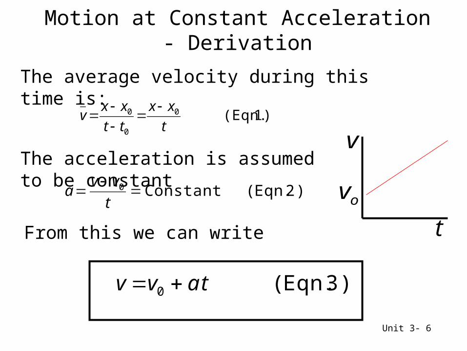
Motion at Constant Acceleration - Derivation

1)(Eqn.0

0

0

t

xx

tt

xxv

) 2 Eqn.(Constant0

t

vva

The average velocity during this time is:

The acceleration is assumed to be constant

From this we can write

) 3 Eqn. (0 tavv

t

v

ov

Unit 3- 6

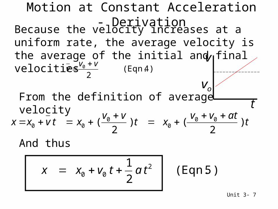
Motion at Constant Acceleration - DerivationBecause the velocity increases at a uniform rate, the average velocity is the average of the initial and final velocities

)4Eqn.(2

0 vvv

From the definition of average velocity

tatvv

xtvv

xtvxx )2

()2

( 000

000

And thus

)5Eqn.(2

1 200 tatvxx

t

v

ov

Unit 3- 7

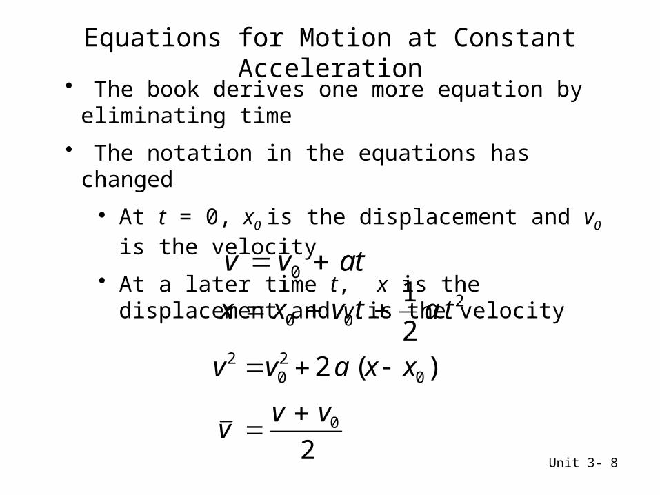
Equations for Motion at Constant Acceleration• The book derives one more equation by eliminating time

• The notation in the equations has changed

• At t = 0, x0 is the displacement and v0 is the velocity

• At a later time t, x is the displacement and v is the velocity

tavv 0

200 2

1tatvxx

)(2 020

2 xxavv

20vv

v

Unit 3- 8

0

2

0

2 2 xxavv

)(20

2

0

2

xx

vva

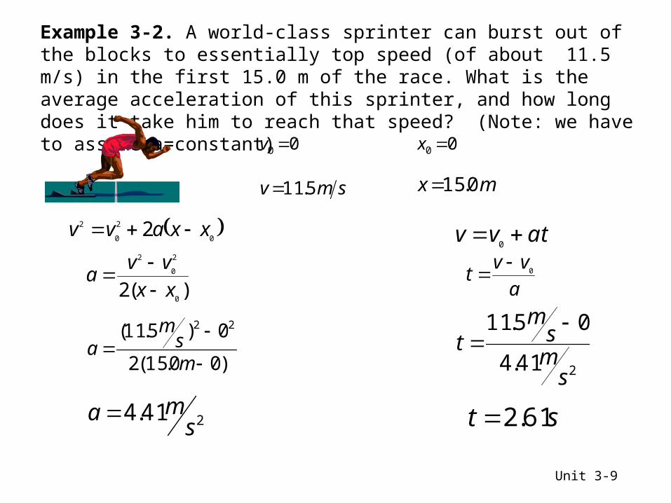
Example 3-2. A world-class sprinter can burst out of the blocks to essentially top speed (of about 11.5 m/s) in the first 15.0 m of the race. What is the average acceleration of this sprinter, and how long does it take him to reach that speed? (Note: we have to assume a=constant)

)00.15(2

0)5.11( 22

ms

ma

241.4s

ma

atvv 0

a

vvt 0

241.4

05.11

sms

mt

st 61.2

Unit 3-9

00 v

smv 5.11

00 x

mx 0.15

Graphical Analysis of Linear Motion

t

xslope

Unit 2 - 10

• Consider the graph of x vs. t. The graph is a straight line, which means the slope is constant.

• The slope of the line is the rise (Δy) over the run (Δx).

t

xv

• If we compare this with the definition of velocity,

we see that the slope of the x vs. t graph is the velocity.

Graphical Analysis of Linear Motion

t

xv

0t

lim

t

va

0t

lim

v is the slope of position vs. time graph. Since the graph is not linear, we draw a tangent line at each point and find slope of the tangent line.

Thus a is the slope of velocity vs. time graph.

Unit 3- 11

The graphs describe the motion of a car whose velocity is changing:

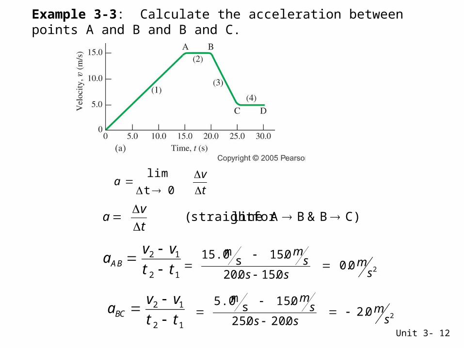
Example 3-3: Calculate the acceleration between points A and B and B and C.

t

va

0t

lim

C) B & B A for linestraight (

t

va

20.00.150.20

0.15sm15.0

sm

sss

m

12

12

tt

vva BA

20.20.200.25

0.15sm5.0

sm

sss

m

12

12

tt

vvaBC

Unit 3- 12

2

00 2

1tatvxx

tttt

tsmx t )25(

200 2

1tatvxx cccc

Example 3-4. A truck going at a constant speed of 25 m/s passes a car at rest. The instant the truck passes the car, the car begins to accelerate at a constant 1.00 m / s2. How long does it take for the car to catch up with the truck.

How far has the car traveled when it catches the truck?

22 )0.1(

2

1t

smx c

When the car catches the truck:tc

xx

tsmts

m )25()0.1(2

1 22

smts

m 25)0.1(2

12

st 50

22 )50)(0.1(

2

1ss

mxc m1250

Unit 3- 13

Example 3-4: Graphical Interpretation

In order to understand the solution to example 4, we can graph the two equations:

22 )0.1(

2

1t

smx c

tsmx t )25(

• The graph of the truck (red) is linear because the velocity is constant.• The car is accelerating so its graph (blue) is quadratic.• The two curves intersect at t = 50 s which agrees with the solution.• They intersect at x ~ 1250 m which also agrees.• The slopes of the two graphs at t = 50 s indicate that the car is traveling twice

as fast as the truck. Unit 3- 14

Unit 3 Appendix

Unit 03- 15

Photo and Clip Art Credits

Some figures electronically reproduced by permission of Pearson Education, Inc., Upper Saddle River, New Jersey Giancoli, PHYSICS,6/E © 2004.

Slide 3-2 Drawing:Copyright © Pearson Prentice Hall, Inc, reproduced with permission3-9 Sprinter: Microsoft Clipart Collection, reproduced under general license for educational purposes.4-10 Graphs: Copyright © Pearson Prentice Hall, Inc, reproduced with permission4-11 Graph: Copyright © Pearson Prentice Hall, Inc, reproduced with permission4-4 Photo:Copyright © Pearson Prentice Hall, Inc, reproduced with permission4-4 Graph: Copyright © Pearson Prentice Hall, Inc, reproduced with permission4-5, 6, 7 Soccer Kicker: Microsoft Clipart Collection, reproduced under general license for educational purposes.4-8, 9 Photo of Leaning Tower of Pisa: Microsoft Clipart Collection, reproduced under general license for educational purposes.

Quadratic Equation

Unit 3- 16

a

cabbx

2

42

A quadratic equation is a polynomial equation of the second degree (one term is squared). The general form of a quadratic equation is

02 cxbxawhere a, b and c are constants and a is not equal to zero. You will need to arrange your equation in this form in order to determine the numeric value of a, b and c. Often this semester, the unknown variable will be t instead of x.

a

cabbx

2

42 a

cabbx

2

42 and

These solutions are usually combined using the ± symbol:

• The solutions can be equal ( if b2 = 4 a c ).• If they are not equal, you will often need to select the solution that makes

sense for the problem.

A quadratic equation has two solutions or roots: