UNIT 3: ANALYSIS OF SIMPLE ALGORITHMS - IGNOU - The People's
26
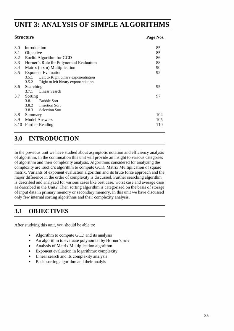
85 UNIT 3: ANALYSIS OF SIMPLE ALGORITHMS Structure Page Nos. 3.0 Introduction 85 3.1 Objective 85 3.2 Euclid Algorithm for GCD 86 3.3 Horner‟s Rule for Polynomial Evaluation 88 3.4 Matrix (n x n) Multiplication 90 3.5 Exponent Evaluation 92 3.5.1 Left to Right binary exponentiation 3.5.2 Right to left binary exponentiation 3.6 Searching 95 3.7.1 Linear Search 3.7 Sorting 97 3.8.1 Bubble Sort 3.8.2 Insertion Sort 3.8.3 Selection Sort 3.8 Summary 104 3.9 Model Answers 105 3.10 Further Reading 110 3.0 INTRODUCTION In the previous unit we have studied about asymptotic notation and efficiency analysis of algorithm. In the continuation this unit will provide an insight to various categories of algorithm and their complexity analysis. Algorithms considered for analyzing the complexity are Euclid‟s algorithm to compute GCD, Matrix Multiplication of square matrix. Variants of exponent evaluation algorithm and its brute force approach and the major difference in the order of complexity is discussed. Further searching algorithm is described and analyzed for various cases like best case, worst case and average case as described in the Unit2. Then sorting algorithm is categorized on the basis of storage of input data in primary memory or secondary memory. In this unit we have discussed only few internal sorting algorithms and their complexity analysis. 3.1 OBJECTIVES After studying this unit, you should be able to: Algorithm to compute GCD and its analysis An algorithm to evaluate polynomial by Horner‟s rule Analysis of Matrix Multiplication algorithm Exponent evaluation in logarithmic complexity Linear search and its complexity analysis Basic sorting algorithm and their analyis
Transcript of UNIT 3: ANALYSIS OF SIMPLE ALGORITHMS - IGNOU - The People's
85
Analysis of simple Algorithms UNIT 3: ANALYSIS OF SIMPLE ALGORITHMS
Structure Page Nos.
3.0 Introduction 85
3.1 Objective 85
3.2 Euclid Algorithm for GCD 86
3.3 Horner‟s Rule for Polynomial Evaluation 88
3.4 Matrix (n x n) Multiplication 90
3.5 Exponent Evaluation 92 3.5.1 Left to Right binary exponentiation
3.5.2 Right to left binary exponentiation
3.6 Searching 95 3.7.1 Linear Search
3.7 Sorting 97 3.8.1 Bubble Sort
3.8.2 Insertion Sort
3.8.3 Selection Sort
3.8 Summary 104
3.9 Model Answers 105
3.10 Further Reading 110
3.0 INTRODUCTION
In the previous unit we have studied about asymptotic notation and efficiency analysis
of algorithm. In the continuation this unit will provide an insight to various categories
of algorithm and their complexity analysis. Algorithms considered for analyzing the
complexity are Euclid‟s algorithm to compute GCD, Matrix Multiplication of square
matrix. Variants of exponent evaluation algorithm and its brute force approach and the
major difference in the order of complexity is discussed. Further searching algorithm
is described and analyzed for various cases like best case, worst case and average case
as described in the Unit2. Then sorting algorithm is categorized on the basis of storage
of input data in primary memory or secondary memory. In this unit we have discussed
only few internal sorting algorithms and their complexity analysis.
3.1 OBJECTIVES
After studying this unit, you should be able to:
Algorithm to compute GCD and its analysis
An algorithm to evaluate polynomial by Horner‟s rule
Analysis of Matrix Multiplication algorithm
Exponent evaluation in logarithmic complexity
Linear search and its complexity analysis
Basic sorting algorithm and their analyis
86
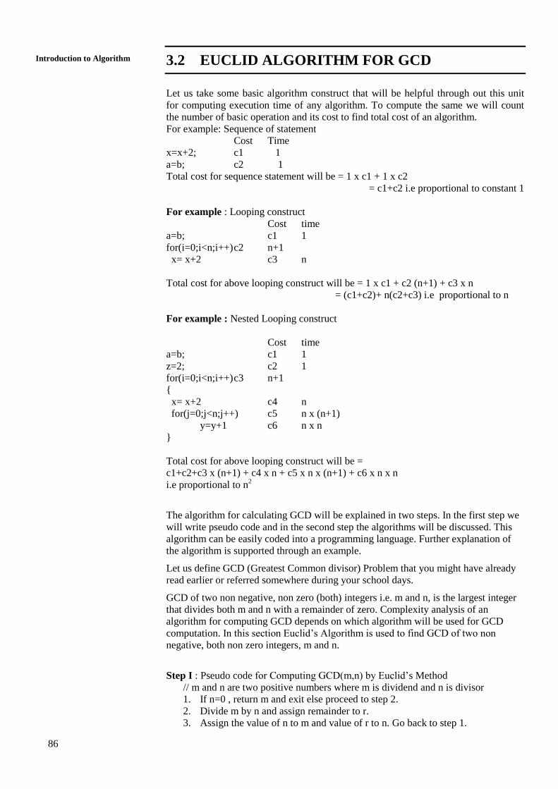
Introduction to Algorithm 3.2 EUCLID ALGORITHM FOR GCD
Let us take some basic algorithm construct that will be helpful through out this unit
for computing execution time of any algorithm. To compute the same we will count
the number of basic operation and its cost to find total cost of an algorithm.
For example: Sequence of statement
Cost Time
x=x+2; c1 1
a=b; c2 1
Total cost for sequence statement will be = 1 x c1 + 1 x c2
= c1+c2 i.e proportional to constant 1
For example : Looping construct
Cost time
a=b; c1 1
for(i=0;i<n;i++) c2 n+1
x= x+2 c3 n
Total cost for above looping construct will be = 1 x c1 + c2 (n+1) + c3 x n
= (c1+c2)+ n(c2+c3) i.e proportional to n
For example : Nested Looping construct
Cost time
a=b; c1 1
z=2; c2 1
for(i=0;i<n;i++) c3 n+1
{
x= x+2 c4 n
for(j=0;j<n;j++) c5 n x (n+1)
y=y+1 c6 n x n
}
Total cost for above looping construct will be =
c1+c2+c3 x (n+1) + c4 x n + c5 x n x (n+1) + c6 x n x n
i.e proportional to n2
The algorithm for calculating GCD will be explained in two steps. In the first step we
will write pseudo code and in the second step the algorithms will be discussed. This
algorithm can be easily coded into a programming language. Further explanation of
the algorithm is supported through an example.
Let us define GCD (Greatest Common divisor) Problem that you might have already
read earlier or referred somewhere during your school days.
GCD of two non negative, non zero (both) integers i.e. m and n, is the largest integer
that divides both m and n with a remainder of zero. Complexity analysis of an
algorithm for computing GCD depends on which algorithm will be used for GCD
computation. In this section Euclid‟s Algorithm is used to find GCD of two non
negative, both non zero integers, m and n.
Step I : Pseudo code for Computing GCD(m,n) by Euclid‟s Method
// m and n are two positive numbers where m is dividend and n is divisor
1. If n=0 , return m and exit else proceed to step 2.
2. Divide m by n and assign remainder to r.
3. Assign the value of n to m and value of r to n. Go back to step 1.
87
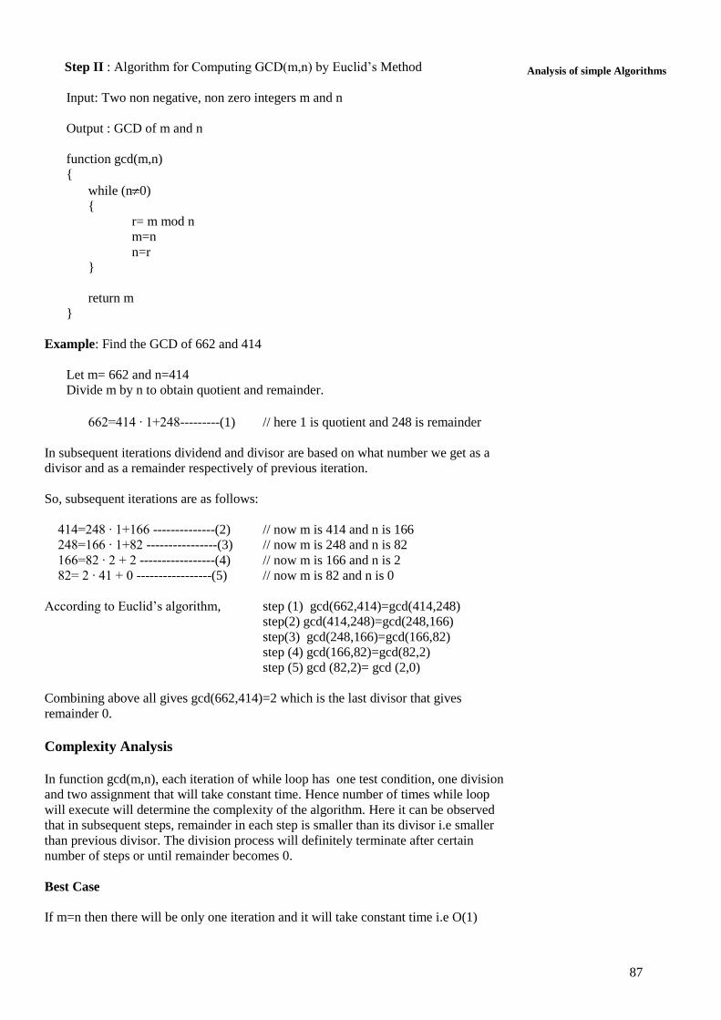
Analysis of simple Algorithms Step II : Algorithm for Computing GCD(m,n) by Euclid‟s Method
Input: Two non negative, non zero integers m and n
Output : GCD of m and n
function gcd(m,n)
{
while (n 0)
{
r= m mod n
m=n
n=r
}
return m
}
Example: Find the GCD of 662 and 414
Let m= 662 and n=414
Divide m by n to obtain quotient and remainder.
662=414 ∙ 1+248---------(1) // here 1 is quotient and 248 is remainder
In subsequent iterations dividend and divisor are based on what number we get as a
divisor and as a remainder respectively of previous iteration.
So, subsequent iterations are as follows:
414=248 ∙ 1+166 --------------(2) // now m is 414 and n is 166
248=166 ∙ 1+82 ----------------(3) // now m is 248 and n is 82
166=82 ∙ 2 + 2 -----------------(4) // now m is 166 and n is 2
82= 2 ∙ 41 + 0 -----------------(5) // now m is 82 and n is 0
According to Euclid‟s algorithm, step (1) gcd(662,414)=gcd(414,248)
step(2) gcd(414,248)=gcd(248,166)
step(3) gcd(248,166)=gcd(166,82)
step (4) gcd(166,82)=gcd(82,2)
step (5) gcd (82,2)= gcd (2,0)
Combining above all gives gcd(662,414)=2 which is the last divisor that gives
remainder 0.
Complexity Analysis
In function gcd(m,n), each iteration of while loop has one test condition, one division
and two assignment that will take constant time. Hence number of times while loop
will execute will determine the complexity of the algorithm. Here it can be observed
that in subsequent steps, remainder in each step is smaller than its divisor i.e smaller
than previous divisor. The division process will definitely terminate after certain
number of steps or until remainder becomes 0.
Best Case
If m=n then there will be only one iteration and it will take constant time i.e O(1)

88
Introduction to Algorithm
Worst Case
If n=1 then there will be m iterations and complexity will be O(m)
If m=1 then there will be n iterations and complexity will be O(n)
Average Case
By Euclid‟s algorithm it is observed that
GCD(m,n) = GCD(n,m mod n) = GCD(m mod n, n mod (m mod n))
Since m mod n = r such that m = nq + r, it follows that r < n, so m > 2r. So after every
two iterations, the larger number is reduced by at least a factor of 2 so there are at
most O(log n) iterations.
Complexity will be O(log n), where n is either the larger or the smaller number.
Check Your Progress 1
1. Find GCD(595,252) by Euclid‟s algorithm.
………………………………………………………………………………………
………………………………………………………………………………………
………………………………………………………………………………………
2. Why Euclid‟s algorithm‟s to compute GCD stops at remained 0?
………………………………………………………………………………………
………………………………………………………………………………………
………………………………………………………………………………………
3.3 HORNER’S RULE FOR POLYNOMIAL
EVALUATION
The algorithm for evaluating a polynomial at a given point using Horner‟s rule will be
explained in two steps. In the first step we will write pseudo code and in the second
step the algorithm will be discussed. This algorithm can be easily coded into any
programming language. Further explanation of the algorithm is supported through an
example.
In this section we will discuss the problem of evaluating a polynomial using Horner‟s
rule. This problem is also a familiar problem. Before discussing the algorithm , let us
define the problem of polynomial evaluation. Consider the polynomial
p(x)=anxn+an-1x
n-1+…..+a1x
1+a0x
0
where a0,a1,…..an-1,an are real numbers and we have to evaluate polynomial at a
specific value for x.
//For Example: p(x)=x2+3x+2
At x=2, p(x) = 22+3.2+2 = 4+6+2=12//
Now, we will discuss Horner‟s rule method for polynomial evaluation.
89
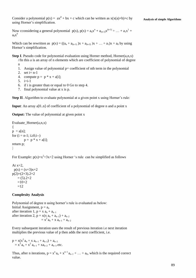
Analysis of simple Algorithms Consider a polynomial p(x) = ax2 + bx + c which can be written as x(x(a)+b)+c by
using Horner‟s simplification.
Now cconsidering a general polynomial p(x), p(x) = anxn + a(n-1)x
(n-1) + … + a1x
1 +
a0x0
Which can be rewritten as p(x) = ((an + a(n-1) )x + a(n-2) )x + … + a1)x + a0 by using
Horner‟s simplification.
Step I. Pseudo code for polynomial evaluation using Horner method, Horner(a,n,x)
//In this a is an array of n elements which are coefficient of polynomial of degree
n
1. Assign value of polynomial p= coefficient of nth term in the polynomial
2. set i= n-1
4. compute p = p * x + a[i];
5. i=i-1
6. if i is greater than or equal to 0 Go to step 4.
7. final polynomial value at x is p.
Step II. Algorithm to evaluate polynomial at a given point x using Horner‟s rule:
Input: An array a[0..n] of coefficient of a polynomial of degree n and a point x
Output: The value of polynomial at given point x
Evaluate_Horner(a,n,x)
{
p = a[n];
for (i = n-1; i 0;i--)
p = p * x + a[i];
return p;
}
For Example: p(x)=x2+3x+2 using Horner „s rule can be simplified as follows
At x=2,
p(x) = (x+3)x+2
p(2)=(2+3).2+2
= (5).2+2
=10+2
=12
Complexity Analysis
Polynomial of degree n using horner‟s rule is evaluated as below:
Initial Assignment, p = an
after iteration 1, p = x an + an–1
after iteration 2, p = x(x an + an–1) + an–2
= x2 an + x an–1 + an–2
Every subsequent iteration uses the result of previous iteration i.e next iteration
multiplies the previous value of p then adds the next coefficient, i.e.
p = x(x2 an + x an–1 + an–2) + an–2
= x3 an + x
2 an–1 + xan–2 + an–3 etc.
Thus, after n iterations, p = xn an + x
n–1 an–1 + … + a0, which is the required correct
value.
90
Introduction to Algorithm
In above function
First step is one initial assignment that takes constant time i.e O(1).
For loop in the algorithm runs for n iterations, where each iteration cost O(1)
as it includes one multiplication, one addition and one assignment which takes
constant time.
Hence total time complexity of the algorithm will be O(n) for a polynomial of
degree n.
Check Your Progress 2
1. Evaluate p(x)= 3x4+2x
3-5x+7 at x=2 using Horne‟s rule. Discuss step wise
iterations.
………………………………………………………………………………………
………………………………………………………………………………………
………………………………………………………………………………………
2. Write basic algorithm to evaluate a polynomial and find its complexity. Also
compare its complexity with complexity of Horner‟s algorithm.
………………………………………………………………………………………
………………………………………………………………………………………
………………………………………………………………………………………
3.4 MATRIX (N X N) MULTIPLICATION
Matrix is very important tool in expressing and discussing problems which arise from
real life cases. By managing the data in matrix form it will be easy to manipulate and
obtain more information. One of the basic operations on matrices is multiplication.
In this section matrix multiplication problem is explained in two steps as we have
discussed GCD and Horner‟s Rule in previous section. In the first step we will brief
pseudo code and in the second step the algorithm for the matrix multiplication will be
discussed. This algorithm can be easily coded into any programming language.
Further explanation of the algorithm is supported through an example.
Let us define problem of matrix multiplication formally , Then we will discuss how to
multiply two square matrix of order n x n and find its time complexity. Multiply two
matrices A and B of order nxn each and store the result in matrix C of order nxn.
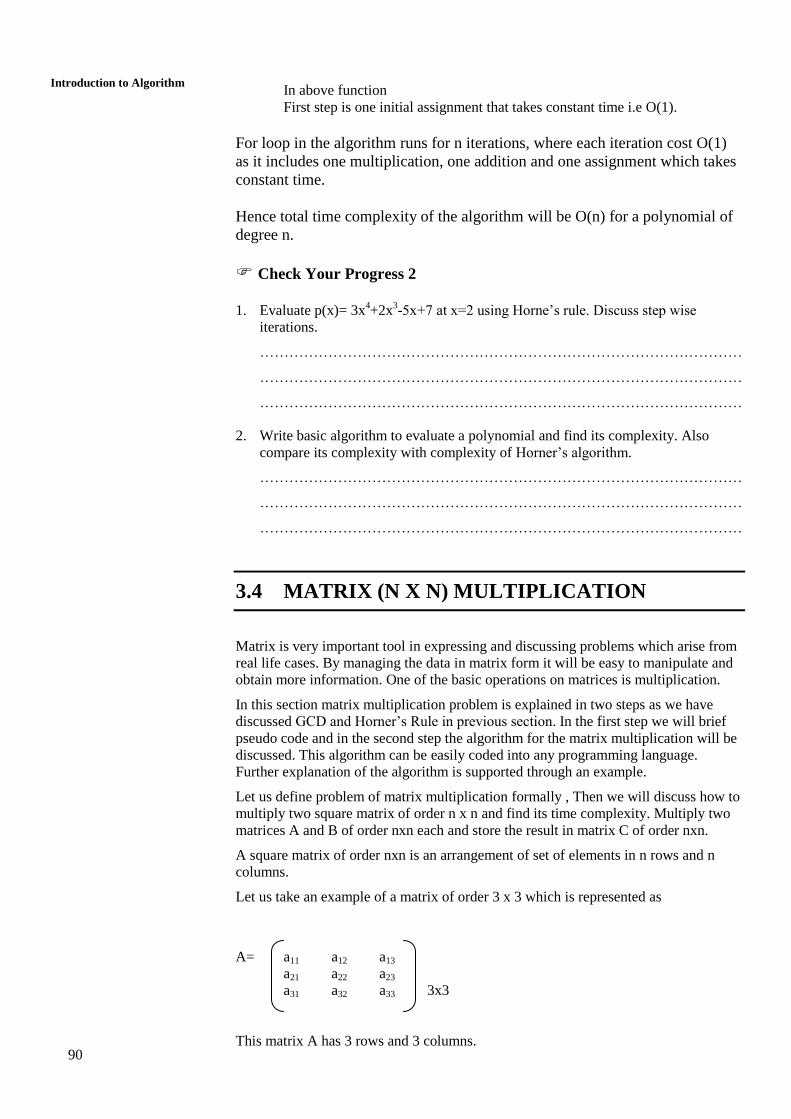
A square matrix of order nxn is an arrangement of set of elements in n rows and n
columns.
Let us take an example of a matrix of order 3 x 3 which is represented as
A= a11 a12 a13
a21 a22 a23
a31 a32 a33 3x3
This matrix A has 3 rows and 3 columns.
91
Analysis of simple Algorithms
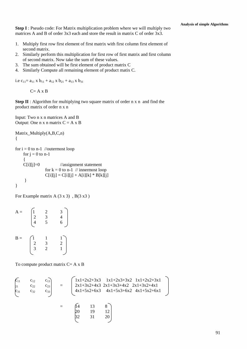
Step I : Pseudo code: For Matrix multiplication problem where we will multiply two
matrices A and B of order 3x3 each and store the result in matrix C of order 3x3.
1. Multiply first row first element of first matrix with first column first element of
second matrix.
2. Similarly perform this multiplication for first row of first matrix and first column
of second matrix. Now take the sum of these values.
3. The sum obtained will be first element of product matrix C
4. Similarly Compute all remaining element of product matix C.
i.e c11= a11 x b11 + a12 x b21 + a13 x b31
C= A x B
Step II : Algorithm for multiplying two square matrix of order n x n and find the
product matrix of order n x n
Input: Two n x n matrices A and B
Output: One n x n matrix C = A x B
Matrix_Multiply(A,B,C,n)
{
for i = 0 to n-1 //outermost loop
for j = 0 to n-1
{
C[i][j]=0 //assignment statement
for k = 0 to n-1 // innermost loop
C[i][j] = C[i][j] + A[i][k] * B[k][j]
}
}
For Example matrix A (3 x 3) , B(3 x3 )
A = 1 2 3
2 3 4
4 5 6
B = 1 1 1
2 3 2
3 2 1
To compute product matrix C= A x B
c11 c12 c13 1x1+2x2+3x3 1x1+2x3+3x2 1x1+2x2+3x1
21 c22 c23 = 2x1+3x2+4x3 2x1+3x3+4x2 2x1+3x2+4x1
c31 c32 c33 4x1+5x2+6x3 4x1+5x3+6x2 4x1+5x2+6x1
= 14 13 8
20 19 12
32 31 20
92
Introduction to Algorithm
Complexity Analysis
First step is, for loop that will be executed n number of times i.e it will take O(n) time.
The second nested for loop will also run for n number of time and will take O(n) time.
Assignment statement inside second for loop will take constant time i.e O(1) as it
includes only one assignment.
The third for loop i.e innermost nested loop will also run for n number of times and
will take O(n ) time . Assignment statement inside third for loop will cost O(1) as it
includes one multiplication, one addition and one assignment which takes constant
time.
Hence, total time complexity of the algorithm will be O(n3) for matrix multiplication
of order nxn.
Check Your Progress 3
1. Write a program in „C‟ to find multiplication of two matrices A[3x3] and B[3 x3].
………………………………………………………………………………………
………………………………………………………………………………………
………………………………………………………………………………………
3.5 EXPONENT EVALUATION
In section 3.4 of this unit we have discussed Horner‟s rule to evaluate polynomial and
its complexity analysis. But computing xn at some point x = a i.e a
n tends to brute
force multiplication of a by itself n times. So computing xn
is most important
operation. It has many applications in various fields for example one of well known
field is cryptography and encryption methods. In this section we will discuss binary
exponentiation methods to compute xn . In this section first we will discuss pseudo
code then we will explain algorithm for computing xn . In this binary representation of
exponent n is used for computation of exponent. Processing of binary string for
exponent n to compute xn can be done by following methods:
left to right binary exponentiation
right to left binary exponentiation
3.6.1 Left to right binary exponentiation
In this method exponent n is represented in binary string. This will be processed from
left to right for exponent computation xn at x=a i.e a
n . First we will discuss its pseudo
code followed by algorithm.
Step I : Pseudo code to compute an by left to right binary exponentiation method
// An array A of size s with binary string equal to exponent n, where s is length of
binary string n
1. Set result =a
2. set i=s-2
3. compute result = result * result
4. if A[i] = 1 then compute result = result * a
5. i=i-1 and if i is less than equal to 0 then go to step 4.
6. return computed value as result.

93
Analysis of simple Algorithms Step II : Algorithm to compute an by left to right binary exponentiation method is as
follows:
Input: an and binary string of length s for exponent n as an array A[s]
Output: Final value of an .
1. result =a
2. for i=s-2 to 0
3. result = result * result
4. if A[i]= 1 then
5. result= result * a
6. return result (i.e an )
Let us take an example to illustrate the above algorithm to compute a17
In this exponent n=17 which is equivalent to binary string 10001
Step by step illustration of the left to right binary exponentiation algorithm for a17
:
s=5
result=a
Iteration 1:
i=3
result=a *a= a2
A[3] 1
Iteration 2:
i=2
result= a2 * a
2 = a
4
A[2] 1
Iteration 3
i=1
result= a4 * a
4 = a
8
A[1] 1
Iteration 4
i=0
result= a8 * a
8 = a
16
A[0] = 1
result = a16
* a = a17
return a17
In this example total number of multiplication is 5 instead of 16 multiplications in
brute force algorithm i.e n-1
Complexity analysis: This algorithm performs either one multiplication or two
multiplications in each iteration of a for loop in line no. 2 of the algorithm.
Hence
Total number of multiplications in the algorithm for computing an will be in the range
of s-1 ≤ f(n) ≤ 2(s-1) where s is length of the binary string equivalent to exponent n
and f is function that represent number of multiplication in terms of exponent n. So
94
Introduction to Algorithm complexity of the algorithm will be O(log2 n) As n can be representation in binary by
using maximum of s bits i.e n=2s which further implies s= O(log2 n)
3.6.2 Right to left binary exponentiation
In right to left binary exponentiation to compute an , processing of bits will start from
least significant bit to most significant bit.
Step I : Pseudo code to compute an by right to left binary exponentiation method
// An array A of size s with binary string equal to exponent n, where s is length of
binary string n
1. Set x =a
2. if A[0]= 1 then set result =a
3. else set result =1
4. Initialize i=1
5. compute x = x * x
6. if A[i] = 1 then compute result = result * x
7. Increment i by 1 as i=i+1 and if i is less than equal to s-1 then go to step 4.
8. return computed value as result.
Step II : Algorithm to compute an by right to left binary exponentiation method
algorithm is as follows:
Input: an and binary string of length s for exponent n as an array A[s]
Output: Final value of an.
1. x=a
2. if A[0]=1 then
3. result = a
4. else
5. result=1
6. for i= 1 to s-1
7. x= x * x
8. if A[i]=1
9. result= result * x
10. return result (i.e an )
Let us take an example to illustrate the above algorithm to compute a17
In this exponent n=17 which is equivalent to binary string 10001
Step by step illustration of the right to left binary exponentiation algorithm for a17
:
s=5, the length of binary string of 1‟s and 0‟s for exponent n
Since A[0] =1 , result=a
Iteration 1:
i=1
x=a *a= a2
A[1] 1
Iteration 2:
i=2
x= a2 * a
2 = a
4
95
Analysis of simple Algorithms A[2] 1
Iteration 3
i=3
x= a4 * a
4 = a
8
A[3] 1
Iteration 4
i=4
x= a8 * a
8 = a
16
A[4] = 1
result = result * x = a * a16
= a17
return a17
In this example total number of multiplication is 5 instead of 16 multiplication in
brute force algorithm i.e n-1
Complexity analysis: This algorithm performs either one multiplication or two
multiplications in each iteration of for loop as shown in line no. 6.
Hence
Total number of multiplications in the algorithm for computing an will be in the range
of s-1 ≤ f(n) ≤ 2(s-1) where s is length of the binary string equivalent to exponent n
and f is function that represent number of multiplication in terms of exponent n. So
complexity of the algorithm will be O(log2 n) As n can be representation in binary by
using maximum of s bits i.e n=2s which further implies s= O(log2 n)
From the above discussion we can conclude that the complexity for left to right binary
exponentiation and right to left binary exponentiation is logarithmic in terms of
exponent n.
Check Your Progress 4
1. Compute a283
using left to right and right to left binary exponentiation.
………………………………………………………………………………………
………………………………………………………………………………………
………………………………………………………………………………………
3.6 SEARCHING
Computer system is generally used to store large amount of data. For accessing a data
item from a large data set based on some criteria/condition searching algorithms are
required. Many algorithms are available for searching a data item from large data set
stored in a computer viz. linear search, binary search. In this section we will discuss
the performance of linear search algorithm. Binary search will be discussed in the
Block-2. In the next section we will examine how long the linear search algorithm will
take to find a data item/key in the data set.
96
Introduction to Algorithm
3.7.1 Linear Search
Linear searching is the algorithmic process of finding a particular data item/key
element in a large collection of data items. Generally search process will return the
value as true/false whether the searching item/element is found/present in data set or
not?
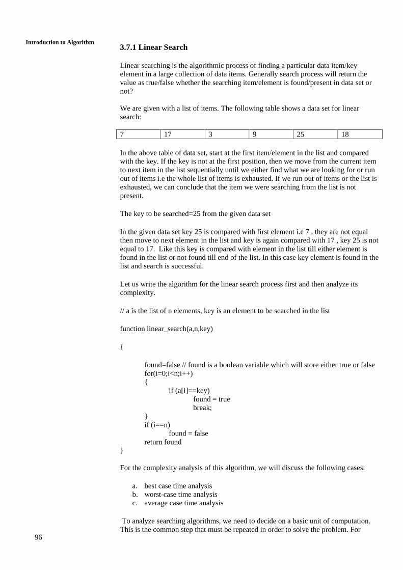
We are given with a list of items. The following table shows a data set for linear
search:
7 17 3 9 25 18
In the above table of data set, start at the first item/element in the list and compared
with the key. If the key is not at the first position, then we move from the current item
to next item in the list sequentially until we either find what we are looking for or run
out of items i.e the whole list of items is exhausted. If we run out of items or the list is
exhausted, we can conclude that the item we were searching from the list is not
present.
The key to be searched=25 from the given data set
In the given data set key 25 is compared with first element i.e 7 , they are not equal
then move to next element in the list and key is again compared with 17 , key 25 is not
equal to 17. Like this key is compared with element in the list till either element is
found in the list or not found till end of the list. In this case key element is found in the
list and search is successful.
Let us write the algorithm for the linear search process first and then analyze its
complexity.
// a is the list of n elements, key is an element to be searched in the list
function linear_search(a,n,key)
{
found=false // found is a boolean variable which will store either true or false
for(i=0;i<n;i++)
{
if (a[i]==key)
found = true
break;
}
if (i==n)
found = false
return found
}
For the complexity analysis of this algorithm, we will discuss the following cases:
a. best case time analysis
b. worst-case time analysis
c. average case time analysis
To analyze searching algorithms, we need to decide on a basic unit of computation.
This is the common step that must be repeated in order to solve the problem. For
97
Analysis of simple Algorithms searching, comparison operation is the key operation in the algorithm so it makes
sense to count the number of comparisons performed. Each comparison may or may
not discover the item we are looking for. If the item is not in the list, the only way to
know it is to compare it against every item present.
Best Case:
The best case - we will find the key in the first place we look, at the beginning of the
list i.e the first comparison returns a match or return found as true. In this case we
only require a single comparison and complexity will be O(1).
Worst Case:
In worst case either we will find the key at the end of the list or we may not find the
key until the very last comparison i.e nth comparison. Since the search requires n
comparisons in the worst case, complexity will be O(n).
Average Case:
On average, we will find the key about halfway into the list; that is, we will compare
against n/2 data items. However, that as n gets larger, the coefficients, no matter what
they are, become insignificant in our approximation, so the complexity of the linear
search, is O(n). The average time depends on the probability that the key will be found
in the collection - this is something that we would not expect to know in the majority
of cases. Thus in this case, as in most others, estimation of the average time is of little
utility.
If the performance of the system is crucial, i.e. it's part of a life-critical system, and
then we must use the worst case in our design calculations and complexity analysis as
it tends to the best guaranteed performance.
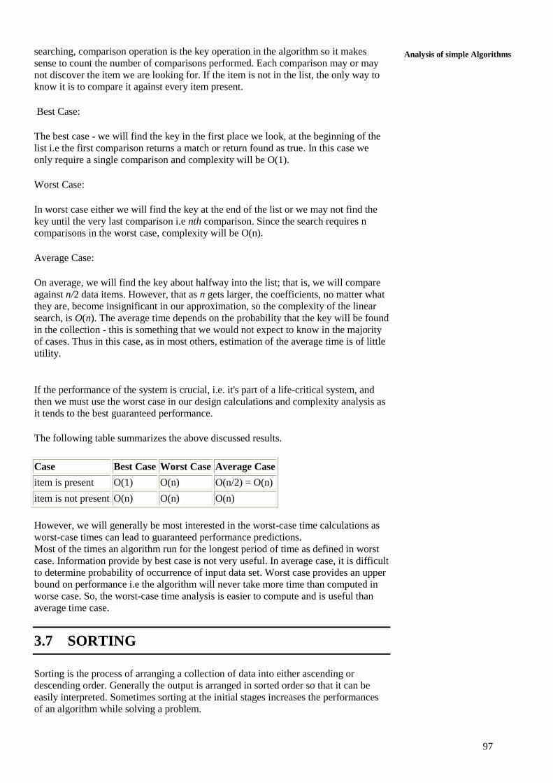
The following table summarizes the above discussed results.
Case Best Case Worst Case Average Case
item is present O(1) O(n) O(n/2) = O(n)
item is not present O(n) O(n) O(n)
However, we will generally be most interested in the worst-case time calculations as
worst-case times can lead to guaranteed performance predictions.
Most of the times an algorithm run for the longest period of time as defined in worst
case. Information provide by best case is not very useful. In average case, it is difficult
to determine probability of occurrence of input data set. Worst case provides an upper
bound on performance i.e the algorithm will never take more time than computed in
worse case. So, the worst-case time analysis is easier to compute and is useful than
average time case.
3.7 SORTING
Sorting is the process of arranging a collection of data into either ascending or
descending order. Generally the output is arranged in sorted order so that it can be
easily interpreted. Sometimes sorting at the initial stages increases the performances
of an algorithm while solving a problem.
98
Introduction to Algorithm Sorting techniques are broadly classified into two categories:
- Internal Sort: - Internal sorts are the sorting algorithms in which the complete data
set to be sorted is available in the computer‟s main memory.
- External Sort: - External sorting techniques are used when the collection of
complete data cannot reside in the main memory but must reside in secondary storage
for example on a disk.
In this section we will discuss only internal sorting algorithms. Some of the internal
sorting algorithms are bubble sort, insertion sort and selection sort. For any sorting
algorithm important factors that contribute to measure their efficiency are the size of
the data set and the method/operation to move the different elements around or
exchange the elements. So counting the number of comparisons and the number of
exchanges made by an algorithm provides useful performance measures. When
sorting large set of data, the number of exchanges made may be the principal
performance criterion, since exchanging two records will involve a lot of time. For
sorting a simple array of integers, the number of comparisons will be more important.
Let us discuss some of internal sorting algorithm and their complexity analysis in next
section.
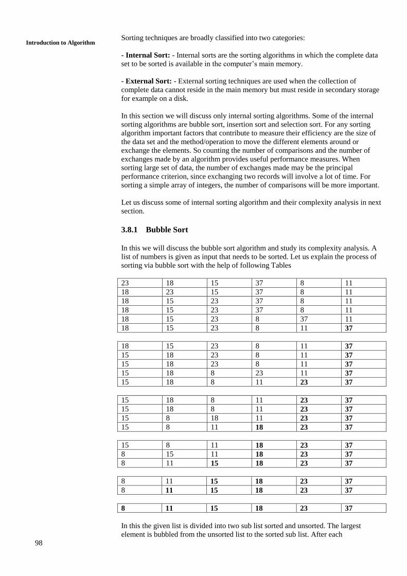
3.8.1 Bubble Sort
In this we will discuss the bubble sort algorithm and study its complexity analysis. A
list of numbers is given as input that needs to be sorted. Let us explain the process of
sorting via bubble sort with the help of following Tables
23 18 15 37 8 11
18 23 15 37 8 11
18 15 23 37 8 11
18 15 23 37 8 11
18 15 23 8 37 11
18 15 23 8 11 37
18 15 23 8 11 37
15 18 23 8 11 37
15 18 23 8 11 37
15 18 8 23 11 37
15 18 8 11 23 37
15 18 8 11 23 37
15 18 8 11 23 37
15 8 18 11 23 37
15 8 11 18 23 37
15 8 11 18 23 37
8 15 11 18 23 37
8 11 15 18 23 37
8 11 15 18 23 37
8 11 15 18 23 37
8 11 15 18 23 37
In this the given list is divided into two sub list sorted and unsorted. The largest
element is bubbled from the unsorted list to the sorted sub list. After each
99
Analysis of simple Algorithms iteration/pass size of unsorted keep on decreasing and size of sorted sub list gets on
increasing till all element of the list comes in the sorted list. With the list of n
elements, n-1 pass/iteration are required to sort. Let us discuss the result of iteration
shown in above tables.
In iteration 1, first and second element of the data set i.e 23 and 18 are compared and
as 23 is greater than 18 so they are swapped. Then second and third element will be
compared i.e 23 and 15 , again 23 is greater than 15 so swapped. Now 23 and 37 is
compared and 23 is less than 37 so no swapping take place. Then 37 and 8 is
compared and 37 is greater than 8 so swapping take place. At the end 37 is compared
with 11 and again swapped. As a result largest element of the given data set i.e 37 is
bubbled at the last position in the data set. Similarly we can perform other iterations of
bubble sort and after n-1 iteration we will get the sorted list.
The algorithm for above sorting method is as below:
// a is the list of n elements to be sorted
function bubblesort(a,n)
{
int i,j,temp,flag=true;
for(i=0; i<n-1 && flag==true; i++) // outer loop
{
flag=false
for(j=0; j<n-i-1; j++) // inner loop
{
if(a[j]>a[j+1])
{
flag=true
temp = a[j]; // exchange
a[j] = a[j+1]; // exchange
a[j+1] = temp; // exchange
}
}
}
}
Complexity analysis of bubble sort is as follows.
Best-case:
When the given data set in an array is already sorted in ascending order the number of
moves/exchanges will be 0, then it will be clear that the array is already in order
because no two elements need to be swapped. In that case, the sort should end, which
takes O(1). The total number of key comparisons will be (n-1) so complexity in best
case will be O(n).
Worst-case:
100
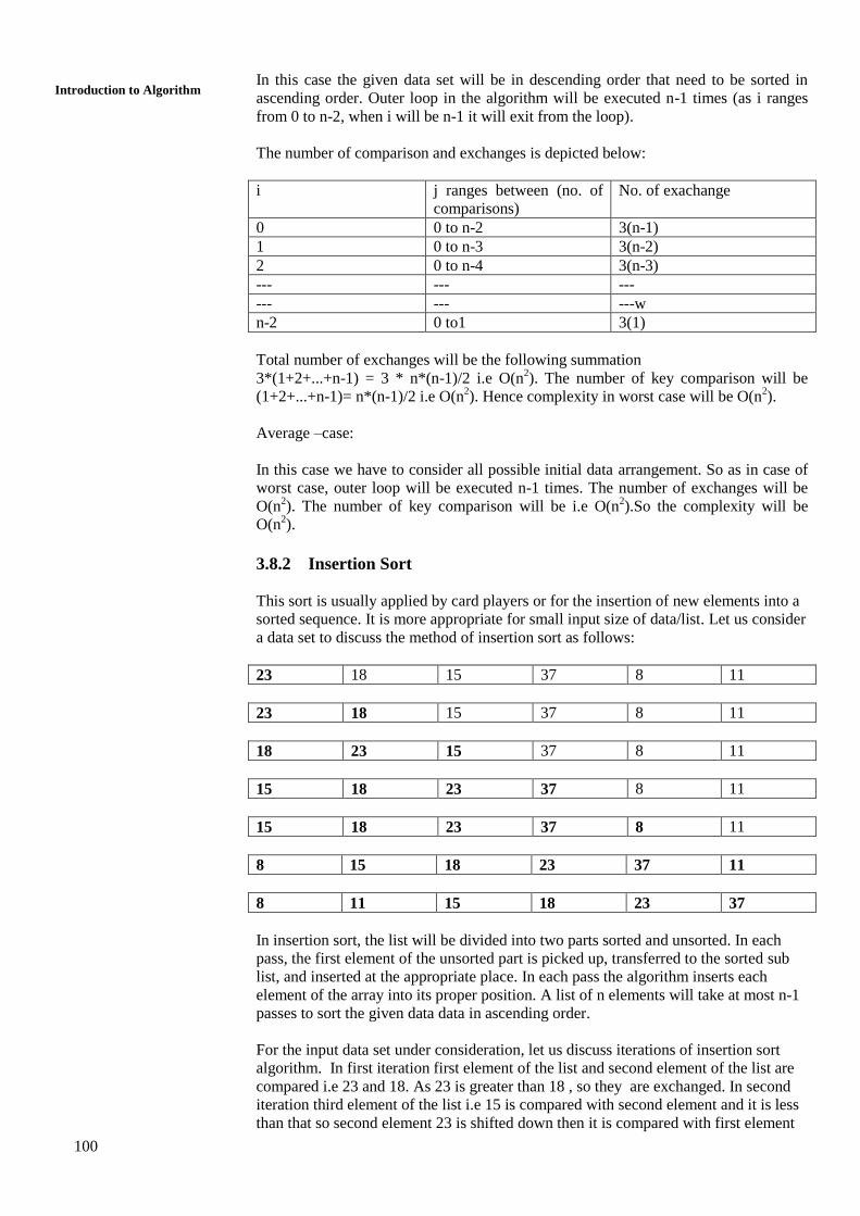
Introduction to Algorithm In this case the given data set will be in descending order that need to be sorted in
ascending order. Outer loop in the algorithm will be executed n-1 times (as i ranges
from 0 to n-2, when i will be n-1 it will exit from the loop).
The number of comparison and exchanges is depicted below:
i j ranges between (no. of
comparisons)
No. of exachange
0 0 to n-2 3(n-1)
1 0 to n-3 3(n-2)
2 0 to n-4 3(n-3)
--- --- ---
--- --- ---w
n-2 0 to1 3(1)
Total number of exchanges will be the following summation
3*(1+2+...+n-1) = 3 * n*(n-1)/2 i.e O(n2). The number of key comparison will be
(1+2+...+n-1)= n*(n-1)/2 i.e O(n2). Hence complexity in worst case will be O(n
2).
Average –case:
In this case we have to consider all possible initial data arrangement. So as in case of
worst case, outer loop will be executed n-1 times. The number of exchanges will be
O(n2). The number of key comparison will be i.e O(n
2).So the complexity will be
O(n2).
3.8.2 Insertion Sort
This sort is usually applied by card players or for the insertion of new elements into a
sorted sequence. It is more appropriate for small input size of data/list. Let us consider
a data set to discuss the method of insertion sort as follows:
23 18 15 37 8 11
23 18 15 37 8 11
18 23 15 37 8 11
15 18 23 37 8 11
15 18 23 37 8 11
8 15 18 23 37 11
8 11 15 18 23 37
In insertion sort, the list will be divided into two parts sorted and unsorted. In each
pass, the first element of the unsorted part is picked up, transferred to the sorted sub
list, and inserted at the appropriate place. In each pass the algorithm inserts each
element of the array into its proper position. A list of n elements will take at most n-1
passes to sort the given data data in ascending order.
For the input data set under consideration, let us discuss iterations of insertion sort
algorithm. In first iteration first element of the list and second element of the list are
compared i.e 23 and 18. As 23 is greater than 18 , so they are exchanged. In second
iteration third element of the list i.e 15 is compared with second element and it is less
than that so second element 23 is shifted down then it is compared with first element
101
Analysis of simple Algorithms and it is less than that also so first element will also be shifted down. Now there is no
more element above that so third element 15 appropriate position is first. This way
rest of the element will get their right position and sorted list will be obtained.
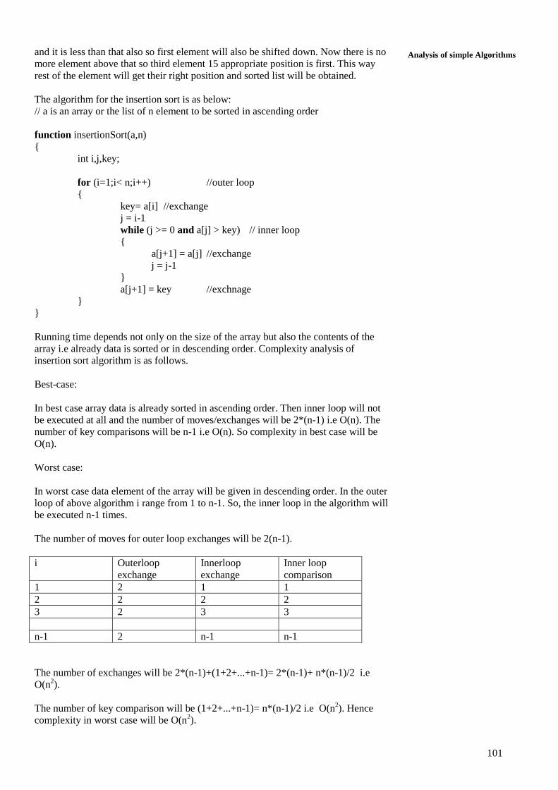
The algorithm for the insertion sort is as below:
// a is an array or the list of n element to be sorted in ascending order
function insertionSort(a,n)
{
int i,j,key;
for (i=1;i< n;i++) //outer loop
{
key= a[i] //exchange
j = i-1
while (j >= 0 and a[j] > key) // inner loop
{
a[j+1] = a[j] //exchange
j = j-1
}
a[j+1] = key //exchnage
}
}
Running time depends not only on the size of the array but also the contents of the
array i.e already data is sorted or in descending order. Complexity analysis of
insertion sort algorithm is as follows.
Best-case:
In best case array data is already sorted in ascending order. Then inner loop will not
be executed at all and the number of moves/exchanges will be 2*(n-1) i.e O(n). The
number of key comparisons will be n-1 i.e O(n). So complexity in best case will be
O(n).
Worst case:
In worst case data element of the array will be given in descending order. In the outer
loop of above algorithm i range from 1 to n-1. So, the inner loop in the algorithm will
be executed n-1 times.
The number of moves for outer loop exchanges will be 2(n-1).
i Outerloop
exchange
Innerloop
exchange
Inner loop
comparison
1 2 1 1
2 2 2 2
3 2 3 3
n-1 2 n-1 n-1
The number of exchanges will be 2*(n-1)+(1+2+...+n-1)= 2*(n-1)+ n*(n-1)/2 i.e
O(n2).
The number of key comparison will be (1+2+...+n-1)= n*(n-1)/2 i.e O(n2). Hence
complexity in worst case will be O(n2).
102
Introduction to Algorithm Average case:
In this case we have to consider all possible initial data arrangement. It is difficult to
figure out the average case. i.e. what will be probability of data set either in mixed /
random input. We can not assume all possible inputs before hand and all cases will be
equally likely. For most algorithms average case is same as the worst case. So as in
case of worst case, outer loop will be executed n-1 times. The number of
moves/assignment will be O(n2). The number of key comparison will be i.e O(n
2). So
the complexity in average case will be O(n2).
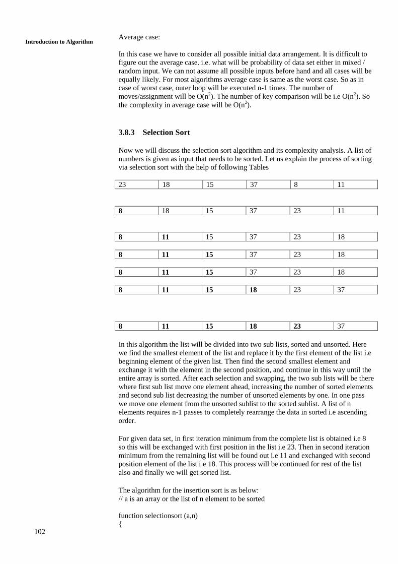
3.8.3 Selection Sort
Now we will discuss the selection sort algorithm and its complexity analysis. A list of
numbers is given as input that needs to be sorted. Let us explain the process of sorting
via selection sort with the help of following Tables
23 18 15 37 8 11
8 18 15 37 23 11
8 11 15 37 23 18
8 11 15 37 23 18
8 11 15 37 23 18
8 11 15 18 23 37
8 11 15 18 23 37
In this algorithm the list will be divided into two sub lists, sorted and unsorted. Here
we find the smallest element of the list and replace it by the first element of the list i.e
beginning element of the given list. Then find the second smallest element and
exchange it with the element in the second position, and continue in this way until the
entire array is sorted. After each selection and swapping, the two sub lists will be there
where first sub list move one element ahead, increasing the number of sorted elements
and second sub list decreasing the number of unsorted elements by one. In one pass
we move one element from the unsorted sublist to the sorted sublist. A list of n
elements requires n-1 passes to completely rearrange the data in sorted i.e ascending
order.
For given data set, in first iteration minimum from the complete list is obtained i.e 8
so this will be exchanged with first position in the list i.e 23. Then in second iteration
minimum from the remaining list will be found out i.e 11 and exchanged with second
position element of the list i.e 18. This process will be continued for rest of the list
also and finally we will get sorted list.
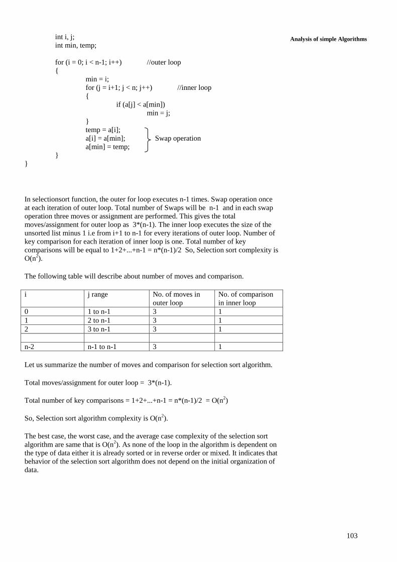
The algorithm for the insertion sort is as below:
// a is an array or the list of n element to be sorted
function selectionsort (a,n)
{
103
Analysis of simple Algorithms int i, j;
int min, temp;
for (i = 0; i < n-1; i++) //outer loop
{
min = i;
for (j = i+1; j < n; j++) //inner loop
{
if (a[j] < a[min])
min = j;
}
temp = a[i];
a[i] = a[min]; Swap operation
a[min] = temp;
}
}
In selectionsort function, the outer for loop executes n-1 times. Swap operation once
at each iteration of outer loop. Total number of Swaps will be n-1 and in each swap
operation three moves or assignment are performed. This gives the total
moves/assignment for outer loop as 3*(n-1). The inner loop executes the size of the
unsorted list minus 1 i.e from i+1 to n-1 for every iterations of outer loop. Number of
key comparison for each iteration of inner loop is one. Total number of key
comparisons will be equal to 1+2+...+n-1 = n*(n-1)/2 So, Selection sort complexity is
O(n2).
The following table will describe about number of moves and comparison.
i j range No. of moves in
outer loop
No. of comparison
in inner loop
0 1 to n-1 3 1
1 2 to n-1 3 1
2 3 to n-1 3 1
n-2 n-1 to n-1 3 1
Let us summarize the number of moves and comparison for selection sort algorithm.
Total moves/assignment for outer loop = 3*(n-1).
Total number of key comparisons = 1+2+...+n-1 = n*(n-1)/2 = O(n2)
So, Selection sort algorithm complexity is O(n2).
The best case, the worst case, and the average case complexity of the selection sort
algorithm are same that is O(n2). As none of the loop in the algorithm is dependent on
the type of data either it is already sorted or in reverse order or mixed. It indicates that
behavior of the selection sort algorithm does not depend on the initial organization of
data.

104
Introduction to Algorithm
Following Table summarizes the above discussed results for different sorting
algorithms.
Algorithm Best Case Worst Case Average Case
Bubble Sort O(n) O(n2) O(n
2)
Insertion Sort O(n) O(n2) O(n
2)
Selection Sort O(n2) O(n
2) O(n
2)
Check Your Progress 5
1. Write advantages and disadvantages of linear search algorithm.
………………………………………………………………………………………
………………………………………………………………………………………
………………………………………………………………………………………
2. Write the iterations for sorting the following list of numbers using bubble sort,
selection sort and insertion sort:
45, 67, 12, 89, 1, 37, 25, 10
………………………………………………………………………………………
………………………………………………………………………………………
………………………………………………………………………………………
………………………………………………………………………………………
………………………………………………………………………………………
………………………………………………………………………………………
3.8 SUMMARY
In this unit various categories of algorithm and their analysis is described like GCD,
matrix multiplication, polynomial evaluation, searching and sorting. For GCD
computation Euclid‟s algorithm is explained and complexity in best case O(1) , worst
case O(m) or O(n) depending upon input and in average case it is O(log n). Horner‟s
rule is discussed to evaluate the polynomial and its complexity is O(n) where n will be
the degree of polynomial. Basic matrix multiplication is explain for finding product of
two matrices of order nxn with time complexity in the order of O(n3). For exponent
evaluation both approaches i.e left to right binary exponentiation and right to left
binary exponentiation is illustrated. Time complexity of these algorithms to compute
xn is O(log n). In large data set to access an element searching algorithm are
required. Here linear search algorithm and its analysis are discussed. Sorting is the
process of arranging a collection of data into either ascending or descending order.
Classification of sorting algorithm based on data storage in primary memory or
secondary memory. Internal sorting algorithms are applied where data to be sorted is
stored in primary memory. Otherwise if input data can not be stored in primary
memory and stored in secondary memory, external sorting techniques are used. In this
unit few internal sorting algorithms like bubble, selection and insertion and their
complexity analysis in worst case, best case and average are discussed.
105
Analysis of simple Algorithms
3.9 MODEL ANSWERS
Check Your Progress 1:
Answers:
1. 595 = 2 x 252 + 91
252 = 2 x 91 +70
91 = 1 x 70 + 21
70 = 3 x 21 + 7
21 = 3 x 7 + 0
GCD(595,252)= 7
According to Euclid‟s algorithm, step (1) gcd(595,252)=gcd(252,91)
step(2) gcd(252,91)=gcd(91, 70)
step(3) gcd(91,70)=gcd(70,21)
step (4) gcd(70,21)=gcd(21,7)
step (5) gcd (21,7)= gcd (7,0)
Combining above all gives gcd(595, 252)=7 which is the last divisor that gives
remainder 0.
2. In Euclid‟s algorithm, at each step remainder decreases at least by 1. So after
finite number of steps remainder must be 0. Non zero remained gives GCD of
given two numbers.
Check Your Progress 2:
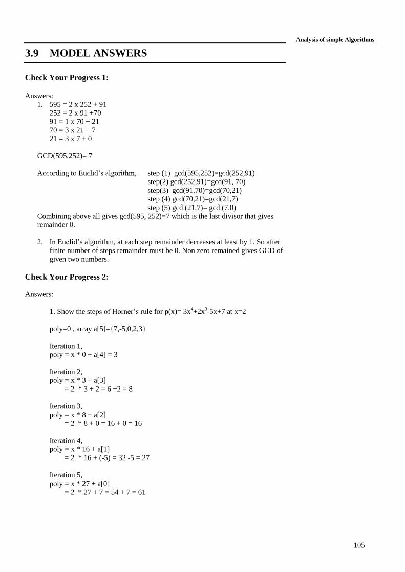
Answers:
1. Show the steps of Horner‟s rule for p(x)= 3x4+2x
3-5x+7 at x=2
poly=0 , array a[5]={7,-5,0,2,3}
Iteration 1,
poly = x * 0 + a[4] = 3
Iteration 2,
poly = x * 3 + a[3]
= 2 * 3 + 2 = 6 +2 = 8
Iteration 3,
poly = x * 8 + a[2]
= 2 * 8 + 0 = 16 + 0 = 16
Iteration 4,
poly = x * 16 + a[1]
= 2 * 16 + (-5) = 32 -5 = 27
Iteration 5,
poly = x * 27 + a[0]
= 2 * 27 + 7 = 54 + 7 = 61

106
Introduction to Algorithm
2. A basic (general) algorithm:
/* a is an array with polynomial coefficient, n is degree of polynomial, x is the point at
which polynomial will be evaluated */
function(a[n], n, x)
{
poly = 0;
for ( i=0; i <= n; i++)
{
result =1;
for (j=0; j<i; j++)
{
result= result * x;
}
poly= poly + result *a[i];
}
return poly.
}
Time Complexity of above basic algorithm is O(n2) where n is the degree of the
polynomial. Time complexity of the Horner‟s rule algorithm is O(n) for a polynomial
of degree n. Basic algorithm is inefficient algorithm in comparison to Horner‟s rule
method for evaluating a polynomial.
Check Your Progress 3:
Answers:
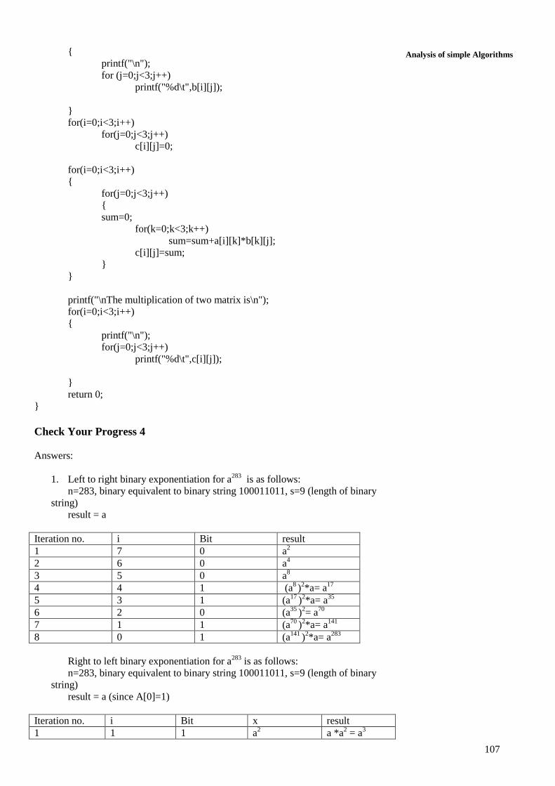
1. C program to find two matrices A[3x3] and B[3x3]
#include<stdio.h>
int main()
{
int a[3][3],b[3][3],c[3][3],i,j,k,sum=0;
printf("\nEnter the First matrix->");
for(i=0;i<3;i++)
for(j=0;j<3;j++)
scanf("%d",&a[i][j]);
printf("\nEnter the Second matrix->");
for(i=0;i<3;i++)
for(j=0;j<3;j++)
scanf("%d",&b[i][j]);
printf("\nThe First matrix is\n");
for(i=0;i<3;i++)
{
printf("\n");
for(j=0;j<3;j++)
{
printf("%d\t",a[i][j]);
}
}
printf("\nThe Second matrix is\n");
for(i=0;i<3;i++)
107
Analysis of simple Algorithms {
printf("\n");
for (j=0;j<3;j++)
printf("%d\t",b[i][j]);
}
for(i=0;i<3;i++)
for(j=0;j<3;j++)
c[i][j]=0;
for(i=0;i<3;i++)
{
for(j=0;j<3;j++)
{
sum=0;
for(k=0;k<3;k++)
sum=sum+a[i][k]*b[k][j];
c[i][j]=sum;
}
}
printf("\nThe multiplication of two matrix is\n");
for(i=0;i<3;i++)
{
printf("\n");
for(j=0;j<3;j++)
printf("%d\t",c[i][j]);
}
return 0;
}
Check Your Progress 4
Answers:
1. Left to right binary exponentiation for a283
is as follows:
n=283, binary equivalent to binary string 100011011, s=9 (length of binary
string)
result = a
Iteration no. i Bit result
1 7 0 a2
2 6 0 a4
3 5 0 a8
4 4 1 (a8 )
2*a= a
17
5 3 1 (a17
)2*a= a
35
6 2 0 (a35
)2= a
70
7 1 1 (a70
)2*a= a
141
8 0 1 (a141
)2*a= a
283
Right to left binary exponentiation for a283
is as follows:
n=283, binary equivalent to binary string 100011011, s=9 (length of binary
string)
result = a (since A[0]=1)
Iteration no. i Bit x result
1 1 1 a2 a *a
2 = a
3
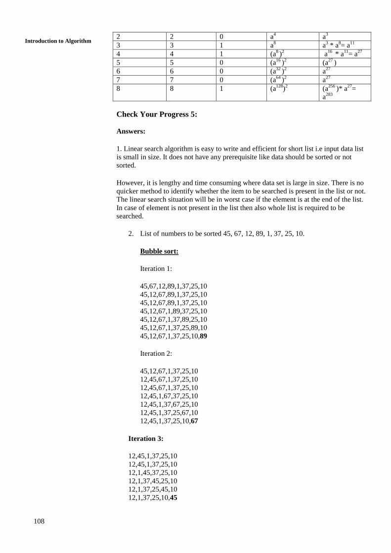
108
Introduction to Algorithm 2 2 0 a
4 a
3
3 3 1 a8 a
3 * a
8= a
11
4 4 1 (a8 )
2 a
16 * a
11= a
27
5 5 0 (a16
)2 (a
27 )
6 6 0 (a32
)2 a
27
7 7 0 (a64
)2 a
27
8 8 1 (a128
)2 (a
256 )* a
27=
a283
Check Your Progress 5:
Answers:
1. Linear search algorithm is easy to write and efficient for short list i.e input data list
is small in size. It does not have any prerequisite like data should be sorted or not
sorted.
However, it is lengthy and time consuming where data set is large in size. There is no
quicker method to identify whether the item to be searched is present in the list or not.
The linear search situation will be in worst case if the element is at the end of the list.
In case of element is not present in the list then also whole list is required to be
searched.
2. List of numbers to be sorted 45, 67, 12, 89, 1, 37, 25, 10.
Bubble sort:
Iteration 1:
45,67,12,89,1,37,25,10
45,12,67,89,1,37,25,10
45,12,67,89,1,37,25,10
45,12,67,1,89,37,25,10
45,12,67,1,37,89,25,10
45,12,67,1,37,25,89,10
45,12,67,1,37,25,10,89
Iteration 2:
45,12,67,1,37,25,10
12,45,67,1,37,25,10
12,45,67,1,37,25,10
12,45,1,67,37,25,10
12,45,1,37,67,25,10
12,45,1,37,25,67,10
12,45,1,37,25,10,67
Iteration 3:
12,45,1,37,25,10
12,45,1,37,25,10
12,1,45,37,25,10
12,1,37,45,25,10
12,1,37,25,45,10
12,1,37,25,10,45
109
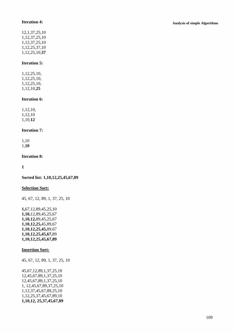
Analysis of simple Algorithms Iteration 4:
12,1,37,25,10
1,12,37,25,10
1,12,37,25,10
1,12,25,37,10
1,12,25,10,37
Iteration 5:
1,12,25,10,
1,12,25,10,
1,12,25,10,
1,12,10,25
Iteration 6:
1,12,10,
1,12,10
1,10,12
Iteration 7:
1,10
1,10
Iteration 8:
1
Sorted list: 1,10,12,25,45,67,89
Selection Sort:
45, 67, 12, 89, 1, 37, 25, 10
1,67,12,89,45,25,10
1,10,12,89,45,25,67
1,10,12,89,45,25,67
1,10,12,25,45,89,67
1,10,12,25,45,89,67
1,10,12,25,45,67,89
1,10,12,25,45,67,89
Insertion Sort:
45, 67, 12, 89, 1, 37, 25, 10
45,67,12,89,1,37,25,10
12,45,67,89,1,37,25,10
12,45,67,89,1,37,25,10
1, 12,45,67,89,37,25,10
1,12,37,45,67,89,25,10
1,12,25,37,45,67,89,10
1,10,12, 25,37,45,67,89
110
Introduction to Algorithm
3.10 FURTHER READINGS
1. T. H. Cormen, C. E. Leiserson, R. L. Rivest, Clifford Stein, “Introduction to
Algorithms”, 2 nd Ed., PHI, 2004.
2. Robert Sedgewick, “Algorithms in C”, 3rd
Edition, Pearson Education, 2004
3. Ellis Horowitz, Sartaj Sahani, Sanguthevar Rajasekaran, “Fundamentals of
Computer algorithms”, 2nd
Edition, Universities Press, 2008
4. Anany Levitin, “Introduction to the Design and Analysis of Algorithm”, Pearson
Education, 2003.