UNIT-2 Angle Modulation Systemmycsvtunotes.weebly.com/uploads/1/0/1/7/10174835/un… · ·...
88
UNIT-2 Angle Modulation System
-
Upload
truongduong -
Category
Documents
-
view
227 -
download
8
Transcript of UNIT-2 Angle Modulation Systemmycsvtunotes.weebly.com/uploads/1/0/1/7/10174835/un… · ·...

UNIT-2 Angle Modulation System

Introduction
• There are three parameters of a carrier that may carry information: – Amplitude
– Frequency
– Phase

Frequency Modulation • Power in an FM signal does not vary with modulation
• FM signals do not have an envelope that reproduces the modulation
• The figure below shows a simplified FM generator
Insert fig. 4.2

Frequency Deviation
• Frequency deviation of the carrier is proportional to the amplitude of the modulating signal as illustrated

Frequency Modulation Index
• Another term common to FM is the modulation index, as determined by the formula:
m
ff
m

Phase Modulation
• In phase modulation, the phase shift is proportional to the instantaneous amplitude of the modulating signal, according to the formula:
m
pe
k

Relationship Between FM and Phase Modulation
• Frequency is the derivative of phase, or, in other words, frequency is the rate of change of phase
• The modulation index is proportional to frequency deviation and inversely proportional to modulating frequency

Modulating Signal Frequency
Insert fig. 4.4

Converting PM to FM
• An integrator can be used as a means of converting phase modulation to frequency modulation

The Angle Modulation Spectrum
• Angle modulation produces an infinite number of sidebands
• These sidebands are separated from the carrier by multiples of fm
• For practical purposes an angle-modulated signal can be considered to be band-limited

Bessel Functions
• FM and PM signals have similar equations regarding composition
• Bessel functions represent normalized voltages for the various components of an AM or PM signal

Bandwidth • For FM, the bandwidth varies with both deviation and
modulating frequency
• Increasing modulating frequency reduces modulation index so it reduces the number of sidebands with significant amplitude
• On the other hand, increasing modulating frequency increases the frequency separation between sidebands
• Bandwidth increases with modulation frequency but is not directly proportional to it

Bandwidth
• Signal bandwidth:
– We can divide signals into two categories: The pure tone signal (the sinusoidal wave, consisting of one frequency component), and complex signals that are composed of several components, or sinusoids of various frequencies.
t (ms)
T=1x10⁻³ s f=1/1x10-3
=1000Hz=1 kHz
0 1
Pure signal

– The bandwidth of a signal composed of components of various frequencies (complex signal) is
the difference between its highest and lowest frequency components, and is expressed in Hertz (Hz) - the same as frequency.
– For example, a square wave may be constructed by adding sine waves of various frequencies:
– The resulting wave resembles a square wave. If more sine waves of other frequencies were
added, the resulting waveform would more closely resemble a square wave – Since the resulting wave contains 2 frequency components, its bandwidth is around 450-
150=300 Hz.
(ms)
150 Hz sine wave
450 Hz sine wave
Approaching a 150
Hz square wave
Pure tone
Pure tone

• Since voice signals are also composed of several components (pure tones) of various frequencies, the bandwidth of a voice signal is taken to be the difference between the highest and lowest frequencies which are 3000 Hz and (close to) 0 Hz
• Although other frequency components above 3000 Hz exist, (they are more prominent in the male voice), an acceptable degradation of voice quality is achieved by disregarding the higher frequency components, accepting the 3kHz bandwidth as a standard for voice communications
Male voice
Female voice
3000 Hz
frequency
component
3000 Hz
frequency
component

• channel bandwidth: – The bandwidth of a channel (medium) is defined to be the range of
frequencies that the medium can support. Bandwidth is measured in Hz – With each transmission medium, there is a frequency range of
electromagnetic waves that can be transmitted: • Twisted pair cable: 0 to 109 Hz (Bandwidth : 109 Hz) • Coax cable: 0 to 1010 Hz (Bandwidth : 1010 Hz) • Optical fiber: 1014 to 1016 Hz (Bandwidth : 1016 -1014 = 9.9x10¹⁵ Hz)
– Optical fibers have the highest bandwidth (they can support electromagnetic waves with very high frequencies, such as light waves)
– The bandwidth of the channel dictates the information carrying capacity of the channel
– This is calculated using Shannon’s channel capacity formula
Increasing bandwidth

Shannon’s Theorem (Shannon’s Limit for Information Capacity)
• Claude Shannon at Bell Labs figured out how much information a channel could theoretically carry:
I = B log2 (1 + S/N)
– Where I is Information Capacity in bits per second (bps)
– B is the channel bandwidth in Hz
– S/N is Signal-to-Noise ratio (SNR: unitless…don’t make into decibel: dB)
Note that the log
is base 2!

Signal-to-Noise Ratio
• S/N is normally measured in dB (decibel). It is a relationship between the signal we want versus the noise that we do not want, which is in the medium.
• It can be thought of as a fractional relationship (that is, before we take the logarithm):
• 1000W of signal power versus 20W of noise power is either: – 1000/20=50 (unitless!)
– or: about 17 dB ==> 10 log10 1000/20 = 16.9897 dB

• The block diagram on the top shows the blocks common to all communication systems
Communication systems
Digital
Analog

We recall the components of a communication
system:
Input transducer: The device that converts a physical signal from source to an electrical, mechanical or electromagnetic signal more suitable for communicating
Transmitter: The device that sends the transduced signal
Transmission channel: The physical medium on which the signal is carried
Receiver: The device that recovers the transmitted signal from the channel
Output transducer: The device that converts the received signal back into a useful quantity

Analog Modulation • The purpose of a communication system is to transmit information signals
(baseband signals) through a communication channel
• The term baseband is used to designate the band of frequencies representing the original signal as delivered by the input transducer
– For example, the voice signal from a microphone is a baseband signal, and contains frequencies in the range of 0-3000 Hz
– The “hello” wave is a baseband signal:

• Since this baseband signal must be transmitted through a communication channel (such as air or cable) using electromagnetic waves, a procedure is needed to shift the range of baseband frequencies to other frequency ranges suitable for transmission; and, a corresponding shift back to the original frequency range after reception. This is called the process of modulation and demodulation
• Remember the radio spectrum:
• For example, an AM radio system transmits electromagnetic waves with frequencies of around a few hundred kHz (MF band)
• The FM radio system operates with frequencies in the range of 88-108 MHz (VHF band)
AM radio FM radio/TV

• Since the baseband signal contains frequencies in the audio frequency range (3 kHz), some form of frequency-band shifting must be employed for the radio system to operate properly
• This process is accomplished by a device called a modulator • The transmitter block in any communications system contains the modulator device • The receiver block in any communications system contains the demodulator device • The modulator modulates a carrier wave (the electromagnetic wave) which has a
frequency that is selected from an appropriate band in the radio spectrum – For example, the frequency of a carrier wave for FM can be chosen from the VHF
band of the radio spectrum – For AM, the frequency of the carrier wave may be chosen to be around a few
hundred kHz (from the MF band of the radio spectrum) • The demodulator extracts the original baseband signal from the received modulated
signal
In Summary: • Modulation is the process of impressing a low-frequency information signal (baseband
signal) onto a higher frequency carrier signal

Basic analog communications system
Modulator
Demodulator
Transmission
Channel
Input
transducer
Transmitter
Receiver
Output
transducer
Carrier
EM waves (modulated
signal)
EM waves (modulated
signal)
Baseband signal
(electrical signal)
Baseband signal
(electrical signal)

Types of Analog Modulation
Amplitude Modulation (AM)
Amplitude modulation is the process of varying the amplitude of a carrier wave in proportion to the amplitude of a baseband signal. The frequency of the carrier remains constant
Frequency Modulation (FM)
Frequency modulation is the process of varying the frequency of a carrier wave in proportion to the amplitude of a baseband signal. The amplitude of the carrier remains constant
Phase Modulation (PM)
Another form of analog modulation technique which we will not discuss

Amplitude Modulation
Carrier wave
Baseband signal
Modulated wave
Amplitude varying-
frequency constant

Frequency Modulation
Carrier wave
Baseband signal
Modulated wave Frequency varying-
amplitude constant
Large
amplitude: high
frequency
Small
amplitude: low
frequency

Carson’s Rule
• Calculating the bandwidth of an FM signal is simple, but tedious using Bessel functions
• Carson’s Rule provides an adequate approximation for determining FM signal bandwidth:
(max)max2 mfB

Variation of FM Signal
Insert fig. 4.9

Narrowband and Wideband FM
• There are no theoretical limits to the modulation index or the frequency deviation of an FM signal
• The limits are a practical compromise between signal-to-noise ratio and bandwidth
• Government regulations limit the bandwidth of FM transmissions in terms of maximum frequency deviation and the maximum modulation frequency

Narrow- and Wideband Signals • Narrowband FM (NBFM) is used for voice transmissions
• Wideband FM (WBFM) is used for most other transmissions
• Strict definition of the term narrowband FM refers to a signal with mf of less than 0.5
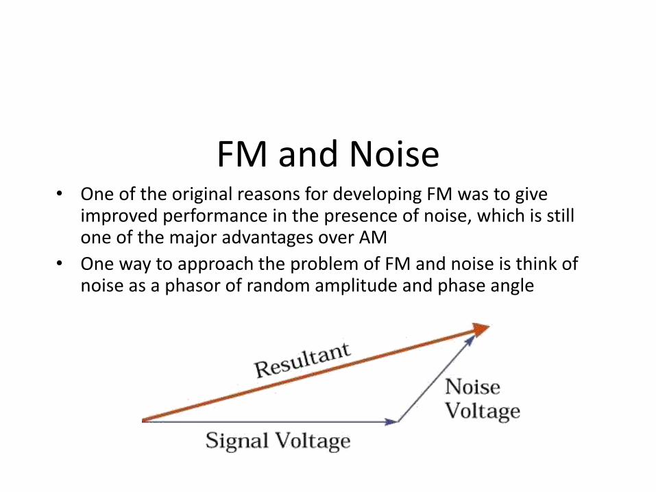
FM and Noise • One of the original reasons for developing FM was to give
improved performance in the presence of noise, which is still one of the major advantages over AM
• One way to approach the problem of FM and noise is think of noise as a phasor of random amplitude and phase angle
Insert fig. 4.10

FM Stereo
• The introduction of FM stereo in 1961 was accomplished in such a way so as to insure compatibility with existing FM monaural systems
• The mono FM receivers must be able to capture the L+R signal of a stereo transmitter

FM Broadcasting Spectra

FM Measurements
• The maximum frequency deviation of an FM transmitter is restricted by law, not by any physical constraint
• Traditional oscilloscope displays are not useful in analyzing FM signals
• A spectrum analyzer is much more useful in determining the qualities of an FM signal

FM Signal Spectrum.
The amplitudes drawn are completely arbitrary, since we have not found any value for Jn() – this sketch is only to illustrate the spectrum.

Generation of FM signals – Frequency Modulation.
An FM demodulator is:
• a voltage-to-frequency converter V/F • a voltage controlled oscillator VCO
In these devices (V/F or VCO), the output frequency is dependent on the input voltage amplitude.

FM Signal Waveforms.
The diagrams below illustrate FM signal waveforms for various inputs
At this stage, an input digital data sequence, d(t), is introduced – the output in this case will be FSK, (Frequency Shift Keying).

FM Signal Waveforms.
Assuming
s0'for
s1'for )(
V
Vtd
s0'for
s1'for
0
1
Vfff
Vfff
cOUT
cOUT
the output ‘switches’ between f1 and f0.

FM Signal Waveforms.
The output frequency varies ‘gradually’ from fc to (fc + Vm), through fc to (fc - Vm) etc.

FM Signal Waveforms.
If we plot fOUT as a function of VIN:
In general, m(t) will be a ‘band of signals’, i.e. it will contain amplitude and frequency variations. Both amplitude and frequency change in m(t) at the input are translated to (just) frequency changes in the FM output signal, i.e. the amplitude of the output FM signal is constant.
Amplitude changes at the input are translated to deviation from the carrier at the output. The larger the amplitude, the greater the deviation.

FM Signal Waveforms.
Frequency changes at the input are translated to rate of change of frequency at the output. An attempt to illustrate this is shown below:

FM Spectrum – Bessel Coefficients.
The FM signal spectrum may be determined from
n
mcncs tnJVtv )cos()()(
The values for the Bessel coefficients, Jn() may be found from graphs or, preferably, tables of ‘Bessel functions of the first kind’.

FM Spectrum – Bessel Coefficients.
In the series for vs(t), n = 0 is the carrier component, i.e. )cos()(0 tJV cc , hence the
n = 0 curve shows how the component at the carrier frequency, fc, varies in amplitude, with modulation index .
Jn()
= 2.4 = 5

FM Spectrum – Bessel Coefficients.
Hence for a given value of modulation index , the values of Jn() may be read off the graph and hence the component amplitudes (VcJn()) may be determined.
A further way to interpret these curves is to imagine them in 3 dimensions
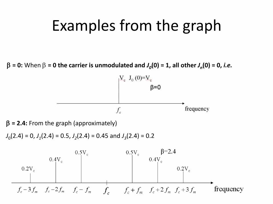
Examples from the graph
= 0: When = 0 the carrier is unmodulated and J0(0) = 1, all other Jn(0) = 0, i.e.
= 2.4: From the graph (approximately)
J0(2.4) = 0, J1(2.4) = 0.5, J2(2.4) = 0.45 and J3(2.4) = 0.2

Significant Sidebands – Spectrum.
As may be seen from the table of Bessel functions, for values of n above a certain value, the values of Jn() become progressively smaller. In FM the sidebands are considered to be significant if Jn() 0.01 (1%).
Although the bandwidth of an FM signal is infinite, components with amplitudes VcJn(), for which Jn() < 0.01 are deemed to be insignificant and may be ignored.
Example: A message signal with a frequency fm Hz modulates a carrier fc to produce FM with a modulation index = 1. Sketch the spectrum.
n Jn(1) Amplitude Frequency
0 0.7652 0.7652Vc fc
1 0.4400 0.44Vc fc+fm fc - fm
2 0.1149 0.1149Vc fc+2fm fc - 2fm
3 0.0196 0.0196Vc fc+3fm fc -3 fm
4 0.0025 Insignificant
5 0.0002 Insignificant

Significant Sidebands – Spectrum.
As shown, the bandwidth of the spectrum containing significant components is 6fm, for = 1.
Significant Sidebands – Spectrum.
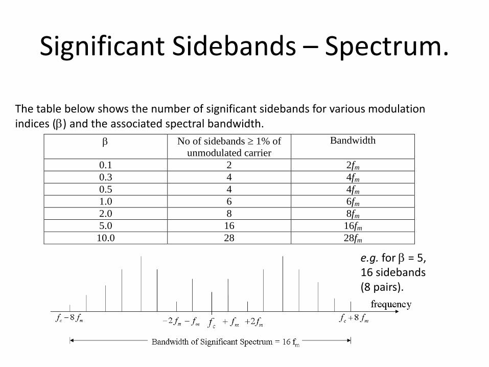
The table below shows the number of significant sidebands for various modulation indices () and the associated spectral bandwidth.
No of sidebands 1% of
unmodulated carrier
Bandwidth
0.1 2 2fm
0.3 4 4fm
0.5 4 4fm
1.0 6 6fm
2.0 8 8fm
5.0 16 16fm
10.0 28 28fm
e.g. for = 5, 16 sidebands (8 pairs).

Carson’s Rule for FM Bandwidth.
An approximation for the bandwidth of an FM signal is given by BW = 2(Maximum frequency deviation + highest modulated frequency)
)(2Bandwidth mc ff Carson’s Rule

Narrowband and Wideband FM
From the graph/table of Bessel functions it may be seen that for small , ( 0.3) there is only the carrier and 2 significant sidebands, i.e. BW = 2fm. FM with 0.3 is referred to as narrowband FM (NBFM) (Note, the bandwidth is the same as DSBAM).
For > 0.3 there are more than 2 significant sidebands. As increases the number of sidebands increases. This is referred to as wideband FM (WBFM).
Narrowband FM NBFM
Wideband FM WBFM

VHF/FM
mc Vf
VHF/FM (Very High Frequency band = 30MHz – 300MHz) radio transmissions, in the band 88MHz to 108MHz have the following parameters:
Max frequency input (e.g. music) 15kHz fm
Deviation 75kHz
Modulation Index 5 m
c
f
f
For = 5 there are 16 sidebands and the FM signal bandwidth is 16fm = 16 x 15kHz = 240kHz. Applying Carson’s Rule BW = 2(75+15) = 180kHz.
Comments FM
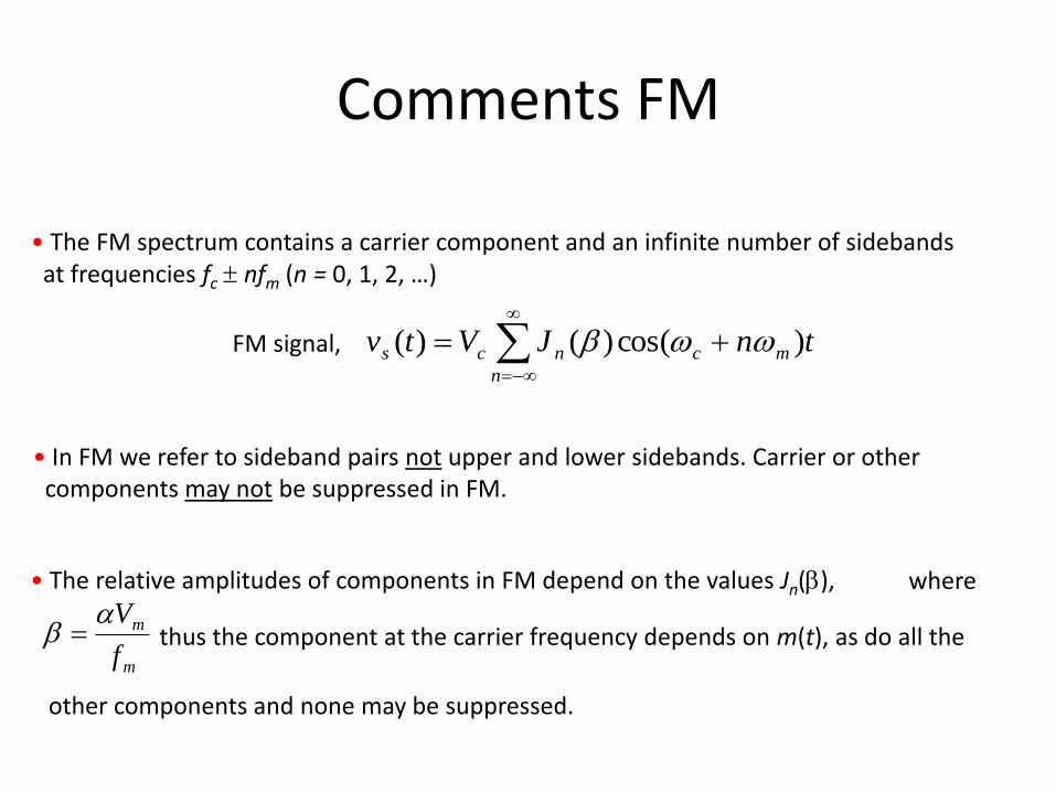
• The FM spectrum contains a carrier component and an infinite number of sidebands at frequencies fc nfm (n = 0, 1, 2, …)
FM signal,
n
mcncs tnJVtv )cos()()(
• In FM we refer to sideband pairs not upper and lower sidebands. Carrier or other components may not be suppressed in FM.
• The relative amplitudes of components in FM depend on the values Jn(), where
m
m
f
V thus the component at the carrier frequency depends on m(t), as do all the
other components and none may be suppressed.

Comments FM
• Components are significant if Jn() 0.01. For <<1 ( 0.3 or less) only J0() and J1() are significant, i.e. only a carrier and 2 sidebands. Bandwidth is 2fm, similar to DSBAM in terms of bandwidth - called NBFM.
• Large modulation index m
c
f
f means that a large bandwidth is required – called
WBFM.
• The FM process is non-linear. The principle of superposition does not apply. When m(t) is a band of signals, e.g. speech or music the analysis is very difficult (impossible?). Calculations usually assume a single tone frequency equal to the maximum input frequency. E.g. m(t) band 20Hz 15kHz, fm = 15kHz is used.
Power in FM Signals.
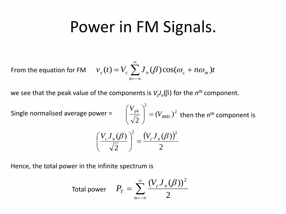
From the equation for FM
n
mcncs tnJVtv )cos()()(
we see that the peak value of the components is VcJn() for the nth component.
Single normalised average power = 2
2
)(2
RMS
pkV
V
then the nth component is
2
)(
2
)(22
ncnc JVJV
Hence, the total power in the infinite spectrum is
Total power
n
ncT
JVP
2
))(( 2
Power in FM Signals.
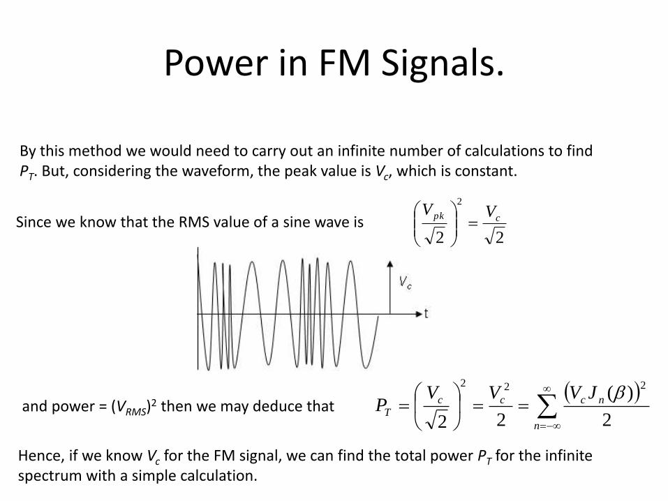
By this method we would need to carry out an infinite number of calculations to find PT. But, considering the waveform, the peak value is Vc, which is constant.
Since we know that the RMS value of a sine wave is 22
2
cpk VV
and power = (VRMS)2 then we may deduce that
n
nccc
T
JVVVP
2
)(
22
222
Hence, if we know Vc for the FM signal, we can find the total power PT for the infinite spectrum with a simple calculation.

Power in FM Signals.
Now consider – if we generate an FM signal, it will contain an infinite number of sidebands. However, if we wish to transfer this signal, e.g. over a radio or cable, this implies that we require an infinite bandwidth channel. Even if there was an infinite channel bandwidth it would not all be allocated to one user. Only a limited bandwidth is available for any particular signal. Thus we have to make the signal spectrum fit into the available channel bandwidth. We can think of the signal spectrum as a ‘train’ and the channel bandwidth as a tunnel – obviously we make the train slightly less wider than the tunnel if we can.

Power in FM Signals.
However, many signals (e.g. FM, square waves, digital signals) contain an infinite number of components. If we transfer such a signal via a limited channel bandwidth, we will lose some of the components and the output signal will be distorted. If we put an infinitely wide train through a tunnel, the train would come out distorted, the question is how much distortion can be tolerated?
Generally speaking, spectral components decrease in amplitude as we move away from the spectrum ‘centre’.
Power in FM Signals.
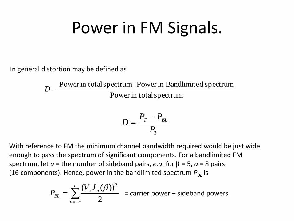
In general distortion may be defined as
spectrum in totalPower
spectrum dBandlimitein Power - spectrum in totalPower D
T
BLT
P
PPD
With reference to FM the minimum channel bandwidth required would be just wide enough to pass the spectrum of significant components. For a bandlimited FM spectrum, let a = the number of sideband pairs, e.g. for = 5, a = 8 pairs (16 components). Hence, power in the bandlimited spectrum PBL is
a
an
ncBL
JVP
2
))(( 2= carrier power + sideband powers.

Power in FM Signals.
Since 2
2
cT
VP
a
an
n
c
a
an
n
cc
JV
JVV
D 2
2
2
22
))((1
2
))((22
Distortion
Also, it is easily seen that the ratio
a
an
n
T
BL JP
PD 2))((
spectrum in totalPower
spectrum dBandlimitein Power = 1 – Distortion
i.e. proportion pf power in bandlimited spectrum to total power =
a
an
nJ 2))((

Example
Consider NBFM, with = 0.2. Let Vc = 10 volts. The total power in the infinite
2
2
cVspectrum = 50 Watts, i.e.
a
an
nJ 2))(( = 50 Watts.
From the table – the significant components are
n Jn(0.2) Amp = VcJn(0.2) Power =
2
)( 2Amp
0 0.9900 9.90 49.005
1 0.0995 0.995 0.4950125
PBL = 49.5 Watts
i.e. the carrier + 2 sidebands contain 99.050
5.49 or 99% of the total power

Example
Distortion = 01.050
5.4950
T
BLT
P
PPor 1%.
Actually, we don’t need to know Vc, i.e. alternatively
Distortion =
1
1
2))2.0((1n
nJ (a = 1)
D = 01.0)0995.0()99.0(1 22
Ratio 99.01))((1
1
2
DJP
P
n
n
T
BL

FM Demodulation –General Principles.
• An FM demodulator or frequency discriminator is essentially a frequency-to-voltage converter (F/V). An F/V converter may be realised in several ways, including for example, tuned circuits and envelope detectors, phase locked loops etc. Demodulators are also called FM discriminators.
• Before considering some specific types, the general concepts for FM demodulation will be presented. An F/V converter produces an output voltage, VOUT which is proportional to the frequency input, fIN.

FM Demodulation –General Principles.
• If the input is FM, the output is m(t), the analogue message signal. If the input is FSK, the output is d(t), the digital data sequence.
• In this case fIN is the independent variable and VOUT is the dependent variable (x and y axes respectively). The ideal characteristic is shown below.
We define Vo as the output when fIN = fc, the nominal input frequency.

FM Demodulation –General Principles.
The gradient f
V
is called the voltage conversion factor
i.e. Gradient = Voltage Conversion Factor, K volts per Hz.
Considering y = mx + c etc. then we may say VOUT = V0 + KfIN from the frequency modulator, and since V0 = VOUT when fIN = fc then we may write
INOUT VKVV 0
where V0 represents a DC offset in VOUT. This DC offset may be removed by level shifting or AC coupling, or the F/V may be designed with the characteristic shown next
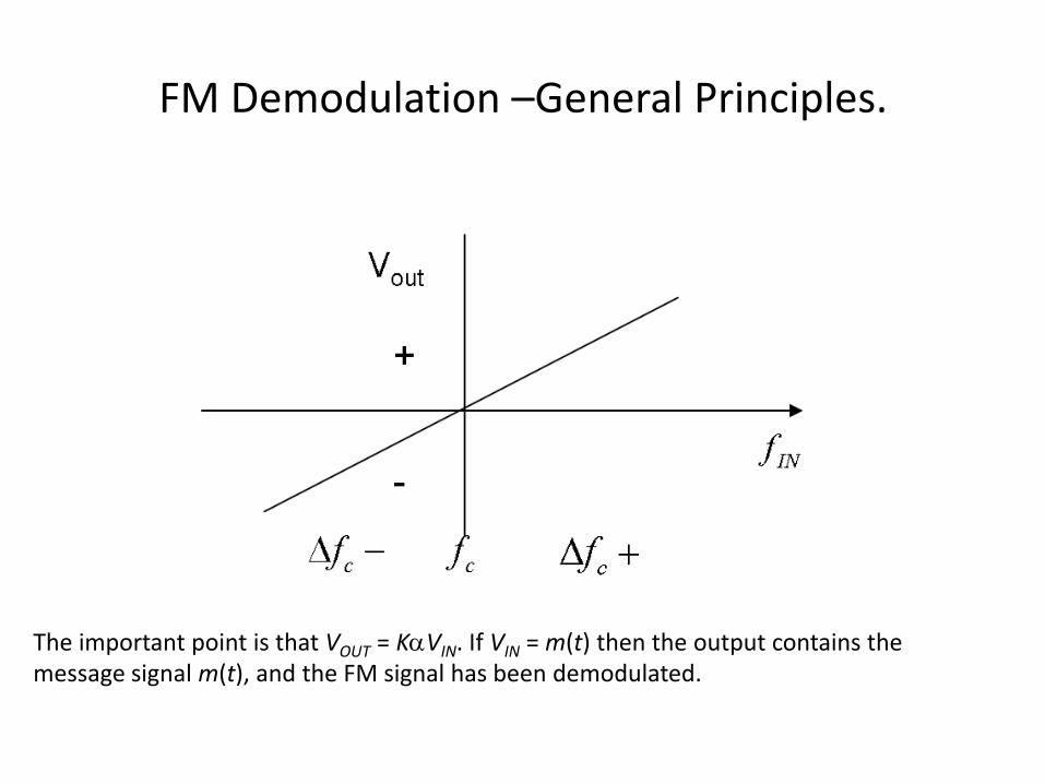
FM Demodulation –General Principles.
The important point is that VOUT = KVIN. If VIN = m(t) then the output contains the message signal m(t), and the FM signal has been demodulated.

FM Demodulation –General Principles.
Often, but not always, a system designed so that
1K , so that K = 1 and
VOUT = m(t). A complete system is illustrated.

FM Demodulation –General Principles.

Methods
Tuned Circuit – One method (used in the early days of FM) is to use the slope of a tuned circuit in conjunction with an envelope detector.
Methods
• The tuned circuit is tuned so the fc, the nominal input frequency, is on the slope, not at the centre of the tuned circuits. As the FM signal deviates about fc on the tuned circuit slope, the amplitude of the output varies in proportion to the deviation from fc. Thus the FM signal is effectively converted to AM. This is then envelope detected by the diode etc to recover the message signal.
• Note: In the early days, most radio links were AM (DSBAM). When FM came along, with its advantages, the links could not be changed to FM quickly. Hence, NBFM was used (with a spectral bandwidth = 2fm, i.e. the same as DSBAM). The carrier frequency fc was chosen and the IF filters were tuned so that fc fell on the slope of the filter response. Most FM links now are wideband with much better demodulators.
• A better method is to use 2 similar circuits, known as a Foster-Seeley Discriminator

Foster-Seeley Discriminator
This gives the composite characteristics shown. Diode D2 effectively inverts the f2 tuned circuit response. This gives the characteristic ‘S’ type detector.

Phase Locked Loops PLL
• A PLL is a closed loop system which may be used for FM demodulation. A full analytical description is outside the scope of these notes. A brief description is presented. A block diagram for a PLL is shown below.
• Note the similarity with a synchronous demodulator. The loop comprises a multiplier, a low pass filter and VCO (V/F converter as used in a frequency modulator).

Phase Locked Loops PLL
• The input fIN is applied to the multiplier and multiplied with the VCO frequency output fO, to produce = (fIN + fO) and = (fIN – fO).
• The low pass filter passes only (fIN – fO) to give VOUT which is proportional to (fIN – fO). • If fIN fO but not equal, VOUT = VIN, fIN – fO is a low frequency (beat frequency) signal to the
VCO.
• This signal, VIN, causes the VCO output frequency fO to vary and move towards fIN. • When fIN = fO, VIN (fIN – fO) is approximately constant (DC) and fO is held constant, i.e locked to
fIN. • As fIN changes, due to deviation in FM, fO tracks or follows fIN. VOUT = VIN changes to drive fO to
track fIN. • VOUT is therefore proportional to the deviation and contains the message signal m(t).

• Armstrong’s Indirect FM

Outline
Two methods of generating FM waves:
Direct method
Indirect Method Armstrong’s FM generator

Direct FM Generation
The carrier freq is directly varied by the input signal
Can be accomplished by Voltage�Controlled
Oscillator (VCO), whose output frequency is
proportional to the voltage of the input signal. A
VCO example: implemented by variable capacitor

Problems of direct FM generator
The carrier freq of VCO tends to drift away.
(Crystal oscillator cannot be used in direct FM: its
freq is too stable, and is difficult to change.)
Feedback freq stabilization circuit is required: The
complexity is increased.
The maximum freq deviation with direct FM is around 5 KHz, too small for wideband FM: Recall: the maximum freq deviation in commercial FM radio is 75kHz.

Indirect FM Generation
First obtain NBFM via a NBPM circuit with crystal oscillator
Change the phase of crystal oscillator is easier than changing its freq.
Then apply frequency multiplier
Increase both the carrier frequency and the freq deviation If necessary, use mixer to concatenate multiple multipliers
Change the carrier frequency, but not the deviation.
Indirect FM is preferred when the stability of carrier frequency is of major concern (e.g., in commercial FM broadcasting)

Recall: Narrow-band FM
if 9f is small: s ( t ) A cos( 2 π f t φ ( t )) c c
s ( t ) A cos( 2 π f t ) A φ ( t ) sin( 2 π f t ) c c c c
φ (t ) x
k π 2 f
Crystal oscillator can be used to get stable frequency (prevent drifting)
But frequency deviation of NBFM is small.
6 To get larger one, use freq multiplier…
Frequency Multipliers
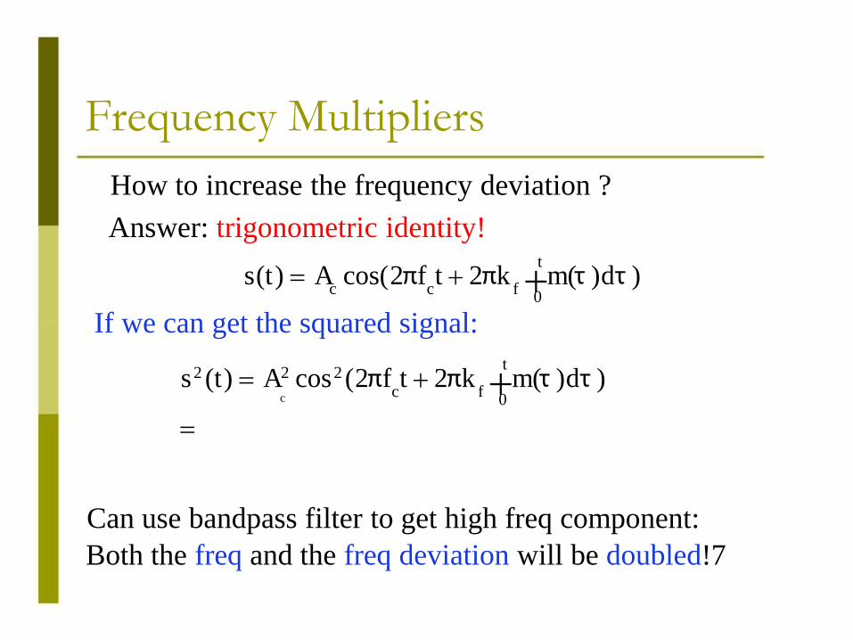
How to increase the frequency deviation ?
Answer: trigonometric identity! t
s ( t ) A cos( 2 π f t 2 π k m ( τ ) d τ ) c c f
0
If we can get the squared signal:
t 2 2 2 s ( t ) A cos ( 2 π f t 2 π k m ( τ ) d τ )
c f c
0
Can use bandpass filter to get high freq component:
Both the freq and the freq deviation will be doubled!7

Frequency Multipliers
If we can get s3(t):
3 2 s ( t ) s ( t ) s ( t )
Can use bandpass filter to get the high freq component:
Both the freq and the freq deviation will be tripled! 8

Freq Multipliers via Nonlinear Circuit
A general nonlinear circuit produces 2 n v ( t ) a s ( t ) a s ( t ) a s ( t )
1 2 n
The highest frequency and the freq sensitivity factor:
nf and nk , respective ly. c f
The bandpass filter:
Center: nfc.
Passband width: determined by Carson’s rule:
2(�f+W) In practice: n = 2, or 3. Larger n is not
efficient. 9 Can concatenate multiple stages to obtain higher orders.

Mixer & Frequency Multiplier
Frequency multiplier increases the freq and deviation
together: How to adjust them individually to get more
flexibilities? Use mixer after frequency multiplier.
freq BPF v(t) s(t) multiplier
2 cos 2 π t f1
Input: s ( t ) A cos( 2 π f t φ ( t )) c c
After freq multiplier:
After multiplying with local freq f1:
Only freq is changed! Freq deviation is untouched.
After BPF: only one freq component is kept. 10

Armstrong’s Indirect FM mixer
BPF
n n 1 2
f 1
Two stages of multiplier and mixer give flexibility between freq and deviation:
The first stage multiplier amplifies both fc and 9f.
The mixer brings down the central freq. The
second stage amplifies fc and 9f again.
11

Example A B
C LPF
n 162 n 30 1 2 f 77 97 MHz 1
NBPM output : f 500 kHz , f 15 432 Hz
Find f and f at A, B, C. (assume low�side tuning)
12

Example A B
C LPF
n 162 n 30 1 2 f 77 97 MHz 1
NBPM output : f 500 kHz , f 15 432 Hz
Point C:
Total multiplier for �f:
This is the same as
The mixer does not affect the freq deviation. 13

Summary
Direct FM generation:
The carrier freq is directly varied by the input
signal Frequency drifting is a problem
Max freq deviation: 5KHz
Indirect FM generation:
NBFM followed by freq multiplier Use
nonlinear circuit to get multiplier Can
use mixer to change the carrier freq
Combination of mixer and multiplier provides flexibilities.
14

AM vs. FM
• AM requires a simple circuit, and is very easy to generate. • It is simple to tune, and is used in almost all short wave broadcasting. • The area of coverage of AM is greater than FM (longer wavelengths
(lower frequencies) are utilized-remember property of HF waves?) • However, it is quite inefficient, and is susceptible to static and other
forms of electrical noise.
• The main advantage of FM is its audio quality and immunity to noise. Most forms of static and electrical noise are naturally AM, and an FM receiver will not respond to AM signals.
• The audio quality of a FM signal increases as the frequency deviation increases (deviation from the center frequency), which is why FM broadcast stations use such large deviation.
• The main disadvantage of FM is the larger bandwidth it requires