
UNIT 1: UNIT 2: CITSTUDENTS - WordPress.com · Control Systems 10ES43 CITSTUDENTS.IN . TEXT BOOK :...
205
Control Systems 10ES43 CITSTUDENTS.IN CONTROL SYSTEMS (Common to EC/TC/EE/IT/BM/ML) Sub Code: 10ES43 IA Marks : 25 Hrs/ Week: 04 Exam Hours : 03 Total Hrs: 52 Marks : 100 UNIT 1: Modeling of Systems: Introduction to Control Systems, Types of Control Systems, Effect of Feedback Systems, Differential equation of Physical Systems -Mechanical systems, Friction, Translational systems (Mechanical accelerometer, systems excluded), Rotational systems, Gear trains, Electrical systems, Analogous systems. 7 Hrs UNIT 2: Block diagrams and signal flow graphs: Transfer functions, Block diagram algebra, Signal Flow graphs (State variable formulation excluded), 6 Hrs UNIT 3: Time Response of feedback control systems: Standard test signals, Unit step response of First and second order systems, Time response specifications, Time response specifications of second order systems, steady123– state errors and error constants. Introduction to PID Controllers (excluding design) 7 Hrs UNIT 4: Stability analysis: Concepts of stability, Necessary conditions for Stability, Routh- stability criterion, Relative stability analysis; more on the Routh stability criterion. 6 Hrs UNIT 5: Root–Locus Techniques: Introduction, The root locus concepts,Construction of root loci 6 Hrs UNIT 6: Frequency domain analysis: Correlation between time and frequency response, Bode plots, Experimental determination of transfer functions, Assessment of relative stability using Bode Plots. Introduction to lead, lag and lead-lag compensating networks (excluding design). 7 Hrs UNIT 7: Stability in the frequency domain: Introduction to Polar Plots, (Inverse Polar Plots excluded) Mathematical preliminaries, Nyquist Stability criterion, Assessment of relative stability using Nyquist criterion, (Systems with transportation lag excluded). 7 Hrs UNIT 8: Introduction to State variable analysis: Concepts of state, state variable and state models for electrical systems, Solution of state equations. 6 Hrs CITSTUDENTS.IN
Transcript of UNIT 1: UNIT 2: CITSTUDENTS - WordPress.com · Control Systems 10ES43 CITSTUDENTS.IN . TEXT BOOK :...

Control Systems 10ES43
CITSTUDENTS.IN
CONTROL SYSTEMS (Common to
EC/TC/EE/IT/BM/ML)
Sub Code: 10ES43 IA Marks : 25
Hrs/ Week: 04 Exam Hours : 03
Total Hrs: 52 Marks : 100
UNIT 1:
Modeling of Systems: Introduction to Control Systems, Types of Control Systems, Effect of Feedback Systems, Differential equation of Physical Systems -Mechanical systems, Friction,
Translational systems (Mechanical accelerometer, systems excluded), Rotational systems, Gear
trains, Electrical systems, Analogous systems. 7 Hrs
UNIT 2:
Block diagrams and signal flow graphs: Transfer functions, Block diagram algebra, Signal Flow graphs (State variable formulation excluded), 6 Hrs
UNIT 3:
Time Response of feedback control systems: Standard test signals, Unit step response of First and second order systems, Time response specifications, Time response specifications of second
order systems, steady123– state errors and error constants. Introduction to PID Controllers
(excluding design) 7 Hrs
UNIT 4:
Stability analysis: Concepts of stability, Necessary conditions for Stability, Routh- stability criterion, Relative stability analysis; more on the Routh stability criterion. 6 Hrs
UNIT 5:
Root–Locus Techniques: Introduction, The root locus concepts,Construction of root loci 6 Hrs
UNIT 6:
Frequency domain analysis: Correlation between time and frequency response, Bode plots,
Experimental determination of transfer functions, Assessment of relative stability using Bode
Plots. Introduction to lead, lag and lead-lag compensating networks (excluding design). 7 Hrs
UNIT 7:
Stability in the frequency domain: Introduction to Polar Plots, (Inverse Polar Plots excluded) Mathematical preliminaries, Nyquist Stability criterion, Assessment of relative stability using
Nyquist criterion, (Systems with transportation lag excluded). 7 Hrs
UNIT 8:
Introduction to State variable analysis: Concepts of state, state variable and state models for
electrical systems, Solution of state equations. 6 Hrs
CITSTUDENTS.IN

Control Systems 10ES43
CITSTUDENTS.IN
TEXT BOOK :
1. J. Nagarath and M.Gopal, ―Control Systems Engineering‖, New Age
International (P) Limited, Publishers, Fourth edition – 2005
REFERENCE BOOKS:
1. “Modern Control Engineering “, K. Ogata, Pearson Education Asia/
PHI, 4th Edition, 2002.
2. “Automatic Control Systems”, Benjamin C. Kuo, John Wiley India
Pvt. Ltd., 8th Edition, 2008.
3. “Feedback and Control System”, Joseph J Distefano III et al.,
Schaum‘s Outlines, TMH, 2nd Edition 2007.
CITSTUDENTS.IN

Control Systems 10ES43
CITSTUDENTS.IN
INDEX SHEET
SL.NO
TOPIC PAGE
NO.
I UNIT 1:Modeling of Systems 1-22
1.1 Introduction to Control Systems, Types of Control Systems
1.2 Effect of Feedback Systems
1.3 Differential equation of Physical Systems -Mechanical systems, Friction
1.4 Translational systems (Mechanical accelerometer, systems excluded)
1.5 Rotational systems , Gear trains
1.6 Electrical systems, Analogous systems
II
UNIT–2 : Block diagrams and signal flow graphs
23-42
2.1 Transfer functions
2.2 Block diagram algebra
2.3 Signal Flow graphs (State variable formulation excluded)
III
UNIT – 3 :Time Response of feedback control systems
3.1 Standard test signals 43-84
3.2 Unit step response of first order systems
3.3 Unit step response of second order systems
3.4 Time response specifications
3.5 Time response specifications of second order systems
3.6 steady23 – state errors and error constants)
3.7 Introduction to PID Controllers (excluding design)
IV
UNIT – 4 : Stability analysis
85-110
4.1 Concepts of stability, Necessary conditions for Stability
4.2 Routh- stability criterion
4.3 Relative stability analysis; More on the Routh stability criterion.
V
UNIT – 5 : Root–Locus Techniques
111-133
5.1 Introduction, The root locus concepts
5.2 Construction of root loci (problems)
VI UNIT – 6 : Frequency domain analysis 134-169
6.1 Correlation between time and frequency response
6.2 Bode plots
6.3 Experimental determination of transfer functions
6.4 Assessment of relative stability using Bode Plots
6.5 Introduction to lead, lag and lead-lag compensating networks (excluding
design)
VII
UNIT – 7 : Stability in the frequency domain 170-182
7.1 Introduction to Polar Plots,(Inverse Polar Plots excluded)
7.2 Mathematical preliminaries
CITSTUDENTS.IN

Control Systems 10ES43
CITSTUDENTS.IN
7.3 Nyquist Stability criterion
7.4 Assessment of relative stability using Nyquist criterion, (Systems with
transportation lag excluded)
VIII UNIT – 8 : Introduction to State variable analysis 183-201
8.1 Concepts of state, state variable
8.2 Concepts of state models for electrical systems
8.3 Solution of state equations
CITSTUDENTS.IN

Control Systems 10ES43
CITSTUDENTS.IN Page 1
UNIT-1
A control system is an arrangement of physical components connected or related in such a
manner as to command, direct, or regulate itself or another system, or is that means by which any
quantity of interest in a system is maintained or altered in accordance with a desired manner.
Any control system consists of three essential components namely input, system and out
put. The input is the stimulus or excitation applied to a system from an external energy source.
A system is the arrangement of physical components and output is the actual response obtained
from the system. The control system may be one of the following type.
1) man made
2) natural and / or biological and 3) hybrid consisting of man made and natural or biological.
Examples:
1) An electric switch is man made control system, controlling flow of electricity.
input : flipping the switch on/off
system : electric switch
output : flow or no flow of current
2) Pointing a finger at an object is a biological control system. input : direction of the object with respect to some direction
system : consists of eyes, arm, hand, finger and brain of a man
output : actual pointed direction with respect to same direction
3) Man driving an automobile is a hybrid system.
input : direction or lane
system : drivers hand, eyes, brain and vehicle output : heading of the automobile.
Classification of Control Systems
Control systems are classified into two general categories based upon the control action which is
responsible to activate the system to produce the output viz.
1) Open loop control system in which the control action is independent of the out put.
2) Closed loop control system in which the control action is some how dependent upon the
output and are generally called as feedback control systems.
Open Loop System is a system in which control action is independent of output. To each
reference input there is a corresponding output which depends upon the system and its operating
conditions. The accuracy of the system depends on the calibration of the system. In the presence
of noise or disturbances open loop control will not perform satisfactorily.
CITSTUDENTS.IN
Control Systems 10ES43
CITSTUDENTS.IN Page 2
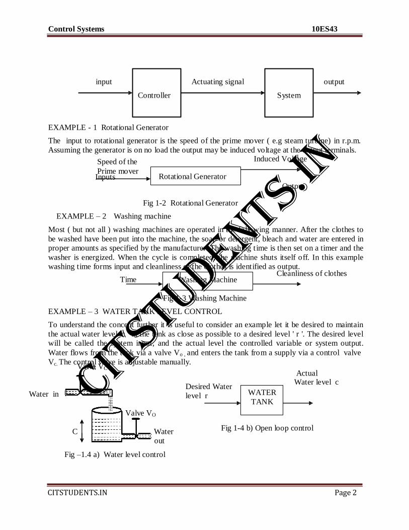
input Actuating signal output
Controller System
EXAMPLE - 1 Rotational Generator
The input to rotational generator is the speed of the prime mover ( e.g steam turbine) in r.p.m.
Assuming the generator is on no load the output may be induced voltage at the output terminals.
Speed of the
Prime mover Inputs
Rotational Generator
Induced Voltage
Output
Fig 1-2 Rotational Generator
EXAMPLE – 2 Washing machine
Most ( but not all ) washing machines are operated in the following manner. After the clothes to
be washed have been put into the machine, the soap or detergent, bleach and water are entered in
proper amounts as specified by the manufacturer. The washing time is then set on a timer and the
washer is energized. When the cycle is completed, the machine shuts itself off. In this example
washing time forms input and cleanliness of the clothes is identified as output. Cleanliness of clothes
Time Washing Machine
Fig 1-3 Washing Machine
EXAMPLE – 3 WATER TANK LEVEL CONTROL
To understand the concept further it is useful to consider an example let it be desired to maintain
the actual water level 'c ' in the tank as close as possible to a desired level ' r '. The desired level
will be called the system input, and the actual level the controlled variable or system output.
Water flows from the tank via a valve Vo , and enters the tank from a supply via a control valve
Vc. The control valve is adjustable manually. Valve VC
Water in
Valve VO
Desired Water
level r
WATER
TANK
Actual Water level c
C Water
out
Fig 1-4 b) Open loop control
Fig –1.4 a) Water level control
CITSTUDENTS.IN

Control Systems 10ES43
CITSTUDENTS.IN Page 3
A closed loop control system is one in which the control action depends on the output. In
closed loop control system the actuating error signal, which is the difference between the input
signal and the feed back signal (out put signal or its function) is fed to the controller.
Reference
input
Error
detector
Actuating
/ error
controller
Control
elements
Forward path
System /
Plant
Controlled
output
Feed back signal
Fig –1.5: Closed loop control system
EXAMPLE – 1 – THERMAL SYSTEM
Feed back elements
To illustrate the concept of closed loop control system, consider the thermal system shown in fig-
6 Here human being acts as a controller. He wants to maintain the temperature of the hot water at
a given value ro
C. the thermometer installed in the hot water outlet measures the actual
temperature C0
C. This temperature is the output of the system. If the operator watches the thermometer and finds that the temperature is higher than the desired value, then he reduc e the amount of steam supply in order to lower the temperature. It is quite possible that that if the temperature becomes lower than the desired value it becomes necessary to increase the amount of steam supply. This control action is based on closed loop operation which involves human being, hand muscle, eyes, thermometer such a system may be called manual feed back system.
Steam
Human operator
Thermometer
Desired hot
water. temp
Brain of
operator (r-c)
Muscles
Actual
Water temp
Co
C
Steam Hot water ro
c + + C
and Valve
Cold water Thermometer
Drain
Fig 1-6 a) Manual feedback thermal system b) Block diagram
EXAMPLE –2 HOME HEATING SYSTEM
The thermostatic temperature control in hour homes and public buildings is a familiar example.
An electronic thermostat or temperature sensor is placed in a central location usually on inside
CITSTUDENTS.IN

Control Systems 10ES43
CITSTUDENTS.IN Page 4
wall about 5 feet from the floor. A person selects and adjusts the desired room temperature ( r )
say 250
C and adjusts the temperature setting on the thermostat. A bimetallic coil in the thermostat is affected by the actual room temperature ( c ). If the room temperature is lower than the desired temperature the coil strip alters the shape and causes a mercury switch to operate a
relay, which in turn activates the furnace fire when the temperature in the furnace air duct system
reaches reference level ' r ' a blower fan is activated by another relay to force the warm air
throughout the building. When the room temperature ' C ' reaches the desired temperature ' r '
the shape of the coil strip in the thermostat alters so that Mercury switch opens. This deactivates
the relay and in turn turns off furnace fire, which in turn the blower.
Desired temp. ro
c +
Relay
switch
Outdoor temp change
(disturbance)
Furnace Blower House
Actual Temp.
Co C
Fig 1-7 Block diagram of Home Heating system.
A change in out door temperature is a disturbance to the home heating system. If the out side
temperature falls, the room temperature will likewise tend to decrease.
CLOSED- LOOP VERSUS OPEN LOOP CONTROL SYSTEMS
An advantage of the closed loop control system is the fact that the use of feedback makes the
system response relatively insensitive to external disturbances and internal variations in systems
parameters. It is thus possible to use relatively inaccurate and inexpensive components to obtain
the accurate control of the given plant, whereas doing so is impossible in the open-loop case.
From the point of view of stability, the open loop control system is easier to build
because system stability is not a major problem. On the other hand, stability is a major problem
in the closed loop control system, which may tend to overcorrect errors that can cause
oscillations of constant or changing amplitude.
It should be emphasized that for systems in which the inputs are known ahead of time and in
which there are no disturbances it is advisable to use open-loop control. closed loop control
systems have advantages only when unpredictable disturbances it is advisable to use open-loop
control. Closed loop control systems have advantages only when unpredictable disturbances and
/ or unpredictable variations in system components used in a closed –loop control system is more
than that for a corresponding open – loop control system. Thus the closed loop control system is
generally higher in cost.
CITSTUDENTS.IN

Control Systems 10ES43
CITSTUDENTS.IN Page 5
Definitions: Systems: A system is a combination of components that act together and perform a certain objective. The system may be physical, biological, economical, etc.
Control system: It is an arrangement of physical components connected or related in a manner
to command, direct or regulate itself or another system.
Open loop: An open loop system control system is one in which the control action is
independent of the output.
Closed loop: A closed loop control system is one in which the control action is somehow
dependent on the output.
Plants: A plant is equipment the purpose of which is to perform a particular operation. Any
physical object to be controlled is called a plant.
Processes: Processes is a natural or artificial or voluntary operation that consists of a series of controlled actions, directed towards a result.
Input: The input is the excitation applied to a control system from an external energy source. The inputs are also known as actuating signals.
Output: The output is the response obtained from a control system or known as controlled
variable.
Block diagram: A block diagram is a short hand, pictorial representation of cause and effect
relationship between the input and the output of a physical system. It characterizes the functional
relationship amongst the components of a control system.
Control elements: These are also called controller which are the components required to
generate the appropriate control signal applied to the plant.
Plant: Plant is the control system body process or machine of which a particular quantity or
condition is to be controlled.
Feedback control: feedback control is an operation in which the difference between the output
of the system and the reference input by comparing these using the difference as a means of
control.
Feedback elements: These are the components required to establish the functional relationship
between primary feedback signal and the controlled output.
Actuating signal: also called the error or control action. It is the algebraic sum consisting of
reference input and primary feedback.
Manipulated variable: it that quantity or condition which the control elements apply to the
controlled system.
Feedback signal: it is a signal which is function of controlled output
Disturbance: It is an undesired input signal which affects the output.
Forward path: It is a transmission path from the actuating signal to controlled output
Feedback path: The feed back path is the transmission path from the controlled output to the
primary feedback signal.
Servomechanism: Servomechanism is a feedback control system in which output is some
mechanical position, velocity or acceleration. Regulator: Regulator is a feedback system in which the input is constant for long time.
Transducer: Transducer is a device which converts one energy form into other
Tachometer: Tachometer is a device whose output is directly proportional to time rate of change
of input.
Synchros: Synchros is an AC machine used for transmission of angular position synchro motor-
receiver, synchro generator- transmitter.
CITSTUDENTS.IN

Control Systems 10ES43
CITSTUDENTS.IN Page 6
Block diagram: A block diagram is a short hand, pictorial representation of cause and effect
relationship between the input and the output of a physical system. It characterizes the functiona l
relationship amongst the components of a control system.
Summing point: It represents an operation of addition and / or subtraction.
Negative feedback: Summing point is a subtractor.
Positive feedback: Summing point is an adder.
Stimulus: It is an externally introduced input signal affecting the controlled output.
Take off point: In order to employ the same signal or variable as an input to more than block or
summing point, take off point is used. This permits the signal to proceed unaltered along several
different paths to several destinations.
Time response: It is the output of a system as a function of time following the application of a
prescribed input under specified operating conditions.
CITSTUDENTS.IN

Control Systems 10ES43
CITSTUDENTS.IN Page 7
DIFFERENTIAL EQUATIONS OF PHYSICAL SYSTEMS
The term mechanical translation is used to describe motion with a single degree of freedom or
motion in a straight line. The basis for all translational motion analysis is Newton‘s second law
of motion which states that the Net force F acting on a body is related to its mass M and
acceleration ‗a‘ by the equation F = Ma
‗Ma‘ is called reactive force and it acts in a direction opposite to that of acceleration. The
summation of the forces must of course be algebraic and thus considerable care must be taken in
writing the equation so that proper signs prefix the forces.
The three basic elements used in linear mechanical translational systems are ( i ) Masses (ii)
springs iii) dashpot or viscous friction units. The graphical and symbolic notations for all three
are shown in fig 1-8
M
Fig 1-8 a) Mass Fig 1-8 b) Spring Fig 1-8 c) Dashpot
The spring provides a restoring a force when a force F is applied to deform a coiled spring a
reaction force is produced, which to bring it back to its freelength. As long as deformation is
small, the spring behaves as a linear element. The reaction force is equal to the product of the
stiffness k and the amount of deformation.
Whenever there is motion or tendency of motion between two elements, frictional forces exist.
The frictional forces encountered in physical systems are usually of nonlinear nature. The
characteristics of the frictional forces between two contacting surfaces often depend on the
composition of the surfaces. The pressure between surfaces, their relative velocity and others.
The friction encountered in physical systems may be of many types
( coulomb friction, static friction, viscous friction ) but in control problems viscous friction,
predominates. Viscous friction represents a retarding force i.e. it acts in a direction opposite to
the velocity and it is linear relationship between applied force and velocity. The mathematical
expression of viscous friction F=BV where B is viscous frictional co-efficient. It should be
realized that friction is not always undesirable in physical systems. Sometimes it may be
necessary to introduce friction intentionally to improve dynamic response of the system. Friction
may be introduced intentionally in a system by use of dashpot as shown in fig 1-9. In
automobiles shock absorber is nothing but dashpot.
CITSTUDENTS.IN

Control Systems 10ES43
CITSTUDENTS.IN Page 8
a b
Applied force
F Piston
The basic operation of a dashpot, in which the housing is filled with oil. If a force f is applied to
the shaft, the piston presses against oil increasing the pressure on side ‗b‘ and decreasing
pressure side ‗a‘ As a result the oil flows from side ‗b‘ to side ‗a‘ through the wall clearance. The
friction coefficient B depends on the dimensions and the type of oil used.
Outline of the procedure
For writing differential equations
1. Assume that the system originally is in equilibrium in this way the often-troublesome
effect of gravity is eliminated.
2. Assume then that the system is given some arbitrary displacement if no distributing force
is present.
3. Draw a freebody diagram of the forces exerted on each mass in the system. There should
be a separate diagram for each mass.
4. Apply Newton‘s law of motion to each diagram using the convention that any force
acting in the direction of the assumed displacement is positive is positive.
5. Rearrange the equation in suitable form to solve by any convenient mathematical means.
Lever
Lever is a device which consists of rigid bar which tends to rotate about a fixed point
called ‗fulcrum‘ the two arms are called ―effort arm‖ and ―Load arm‖ respectively. The lever
bears analogy with transformer
L1 L2
F2 Load
effort F1
Fulcrum
CITSTUDENTS.IN

Control Systems 10ES43
CITSTUDENTS.IN Page 9
It is also called ‗mechanical transformer‘
Equating the moments of the force
F1 L1 = F2 L 2
F 2 = F1 L1
L2
Rotational mechanical system
The rotational motion of a body may be defined as motion about a fixed axis. The variables
generally used to describe the motion of rotation are torque, angular displacement , angular
velocity ( ) and angular acceleration( )
The three basic rotational mechanical components are 1) Moment of inertia J
2 ) Torsional spring 3) Viscous friction.
Moment of inertia J is considered as an indication of the property of an element, which stores the
kinetic energy of rotational motion. The moment of inertia of a given element depends on
geometric composition about the axis of rotation and its density. When a body is rotating a
reactive torque is produced which is equal to the product of its moment
of inertia (J) and angular acceleration and is given by T= J = J d2
d t2
A well known example of a torsional spring is a shaft which gets twist ed when a torque is
applied to it. Ts = K , is angle of twist and K is torsional stiffness.
There is viscous friction whenever a body rotates in viscous contact with another body. This
torque acts in opposite direction so that angular velocity is given by
T = f = f d2
Where = relative angular velocity between two bodies.
d t2
f = co efficient of viscous friction.
Newton‘s II law of motion states
T = J d2 .
d t2
Gear wheel
In almost every control system which involves rotational motion gears are necessary. It is often
necessary to match the motor to the load it is driving. A motor which usually runs at high speed
and low torque output may be required to drive a load at low speed and high torque.
CITSTUDENTS.IN

Control Systems 10ES43
CITSTUDENTS.IN Page 10
+
aring equ
+
(1) and (
= e
e see tha
Driving wheel
N1
N2 Driven wheel
Analogous Systems
Consider the mechanical system shown in fig A and the electrical system shown in fig B
The differential equation for mechanical system is
d2x
M + dt
2
dx
+ B dt
+ K X = f (t) ---------- 1
The differential equation for electrical system is
d2q
d2q
q L + R ---------- 2
dt2 dt
2 c
Comp ations 2) w t for the two systems the differential equations are of
identical form such systems are called ― analogous systems and the terms which occupy the
corresponding positions in differential equations are analogous quantities‖
The analogy is here is called force voltage analogy
Table for conversion for force voltage analogy
Mechanical System Electrical System
Force (torque) Voltage
Mass (Moment of inertia) Inductance
Viscous friction coefficient Resistance
Spring constant Capacitance
CITSTUDENTS.IN

Control Systems 10ES43
CITSTUDENTS.IN Page 11
+
+ K
Displacement Charge
Velocity Current.
Force – Current Analogy
Another useful analogy between electrical systems and mechanical systems is based on force –
current analogy. Consider electrical and mechanical systems shown in fig.
For mechanical system the differential equation is given by
d2x dx
M + B X = f (t) ---------- 1
dt2
dt
For electrical system
C d2x 1 d
+ + + = I ( t )
dt2 R dt
2 L
Comparing equations (1) and (2) we find that the two systems are analogous systems. The
analogy here is called force – current analogy. The analogous quantities are listed.
Table of conversion for force – current analogy
Mechanical System Electrical System
Force( torque) Current
Mass( Moment of inertia) Capacitance
Viscous friction coefficient Conductance
Spring constant Inductance
Displacement Flux
( angular)
Velocity (angular) Voltage
Illustration 1:For a two DOF spring mass damper system obtain the mathematical model where
F is the input x1 and x2 are responses.
CITSTUDENTS.IN

Control Systems 10ES43
CITSTUDENTS.IN Page 12
.
k2 b2 (Damper)
m2 x2 (Response)
Draw the free body diagram for mass
m1 and m2 separately as shown in figure 1.10 (b)
k1
m1
F Figure 1.10 (a)
b1
x1 (Response)
.
Apply NSL for both the masses
separately and get equations as given in
(a) and (b)
. k2 x2 b2 x2 k2 x2 b2 x2
m2 m2
. . x2
k1 x2 k1 x1 b1 x1 b1 x2
. .
k1 (x1-x2) b .
-x ) k1 x2 k1 x1
b1 x1 b1 x2
m1
x1
1 (x1 2
m1
F
F
Figure 1.10 (b)
From NSL F= ma
For mass m1
.. . . m1x1 = F - b1 (x1-x2) - k1 (x1-x2) --- (a)
For mass m2
m .x.
= b (x.
-x.
) + k (x -x ) - b x.
- k x --- (b)
2 2 1 2 1 1 2 1 2 2 2 2
CITSTUDENTS.IN

Control Systems 10ES43
CITSTUDENTS.IN Page 13
K
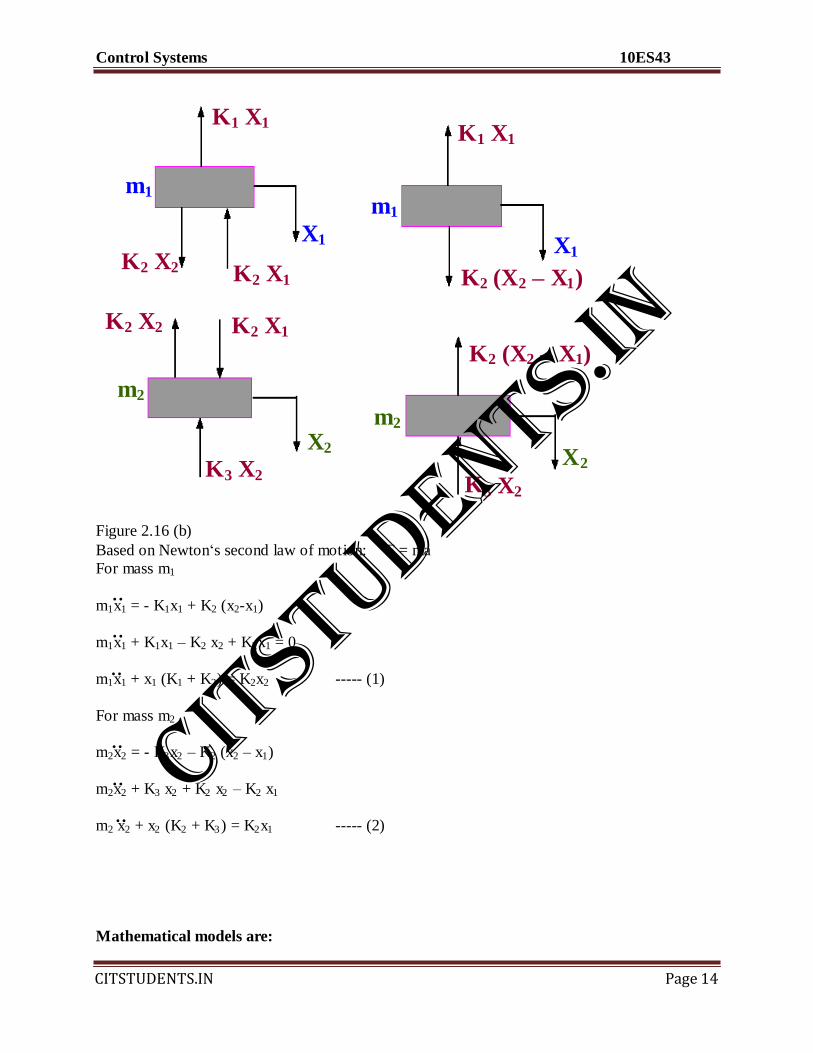
Illustration 2: For the system shown in figure 2.16 (a) obtain the mathematical model if x1 and
x2 are initial displacements.
Let an initial displacement x1 be given to mass m1 and x2 to mass m2.
K1
m1
X1
2
m2
K3 X2
Figure 1.11 (a)
CITSTUDENTS.IN
Control Systems 10ES43
CITSTUDENTS.IN Page 14
X
2 2 3 2 2 2 1
2 2 2 2 3 2 1
2 2 3 2 2 2 2 1
K
K1 X1
K1 X1
m1
m1
X1 X1
K2 X2
K2 X1
K (X
– X )
K2 X2
K2 X1
2 2 1
K2 (X2 – X1)
m2
m2
X2 2
K3 X2
3 X2
Figure 2.16 (b)
Based on Newton‘s second law of motion: F = ma
For mass m1
.. m1x1 = - K1x1 + K2 (x2-x1)
.. m1x1 + K1x1 – K2 x2 + K2x1 = 0
.. m1x1 + x1 (K1 + K2) = K2x2 ----- (1)
For mass m2
m .x.
= - K x – K (x – x )
m .x.
+ K x + K x – K x
m .x.
+ x (K + K ) = K x ----- (2)
Mathematical models are:
CITSTUDENTS.IN

Control Systems 10ES43
CITSTUDENTS.IN Page 15
1 1 1 1 2 2 2
2 2 2 2 3 2 1
m .x.
+ x (K + K ) = K x ----- (1)
m .x.
+ x (K + K ) = K x ----- (2)
1.Write the differential equation relating to motion X of the mass M to the force input u(t)
K1 K2
X
(output)
M U(t)
(input)
2. Write the force equation for the mechanical system shown in figure
X1
K B2
X (output)
F(t)
(input)
M
3. Write the differential equations for the mechanical system shown in figure.
B1
X1 X2
K1
M1
f(t)
f12
M2
f1 f2
4. Write the modeling equations for the mechanical systems shown in figure.
CITSTUDENTS.IN

Control Systems 10ES43
pt o
Xi K X
M M
force f(t) Xo
B
5. For the systems shown in figure write the differential equations and obtain the transfer
functions indicated.
Yk
K F
Xi Xo Xi Xo C
6. Write the differential equation describing the system. Assume the bar through which
force is applied is not flexible, has no mass or moment of inertia, and all
displacements are small.
f(t) b K
X
a M
B
7. Write the equations of motion in terms of given mechanical quantities.
ForcSeJBITf/ De f EKCE 1
X2
Page 16
a b
CITSTUDENTS.IN

Control Systems 10ES43
a small cylind
of inertia J2. T
moment of iner
ylinders are co
ch rotates with
viscous friction Torque T
M1
B1
8. Write the force equations for the mechanical systems shown in figure.
B1
J1
T(t)
9. Write the force equation for the mechanical system shown in figure.
T(t) K
J1 J2
1 2
10. Write the force equation for the mechanical system shown in figure.
1 K1 2 K2
3 K3
11. Torque T(t) is appliJed1to er wJit2h tia J1Jw3hi in a
larger cylinder with moment he two c upled by B1.
SJBIT/ Dept of ECEB1 B2 B3
Page 17
CITSTUDENTS.IN

Control Systems 10ES43
CITSTUDENTS.IN
Page 18
The outer cylinder has viscous friction B2 between it and the reference frame and is restrained by
a torsion spring k. write the describing differential equations.
J2 K
J1 B2
Torque T1, 1 B1
12. The polarized relay shown exerts a force f(t) = Ki. i(t) upon the pivoted bar. Assume the relay
coil has constant inductance L. The left end of the pivot bar is connected to the reference frame through a viscous damper B1 to retard rapid motion of the bar. Assume the bar has negligible
mass and moment of inertia and also that all displacements are small. Write the describing differential equations. Note that the relay coil is not free to move.
13. Figure shows a control scheme for controlling the azimuth angle of an armature controlled
dc. Motion with dc generator used as an amplifier. Determine transfer function
L (s)
CITSTUDENTS.IN

Control Systems 10ES43
CITSTUDENTS.IN
Page 19
. The parameters of the plant are given below.
u (s)
Motor torque constant = KT in N.M /amp
Motor back emf constant = KB in V/ rad / Sec
Generator gain constant Motor to load gear ratio
= =
KG in v/ amp N2
N 1
Resistance of the circuit = R in ohms.
Inductance of the circuit = L in Henry
Moment of inertia of motor = J
Viscous friction coefficient = B
Field resistance = Rf
Field inductance = Lf
14. The schematic diagram of a dc motor control system is shown in figure where Ks is error
detector gain in volt/rad, k is the amplifier gain, Kb back emf constant, Kt is torque
constant, n is the gear train ratio =
2
= Tm Bm = motion friction constant
1
T2
CITSTUDENTS.IN

Control Systems 10ES43
SJBIT/ Dept of ECE Page
Jm = motor inertia, KL = Torsional spring constant JL = load inertia.
15. Obtain a transfer function C(s) /R(s) for the positional servomechanism shown in figure.
Assume that the input to the system is the reference shaft position (R) and the system output is
the output shaft position ( C ). Assume the following constants.
Gain of the potentiometer (error detector ) K1 in V/rad
Amplifier gain ‗ Kp ‘ in V / V
Motor torque constant ‗ KT ‘ in V/ rad
Gear ratio N1 N2
Moment of inertia of load ‗J‘
Viscous friction coefficient ‗f‘
20
CITSTUDENTS.IN

Control Systems 10ES43
CITSTUDENTS.IN
Page 21
16. Find the transfer function E0 (s) / I(s)
C1
I E0
C2 R Output
input
CITSTUDENTS.IN

Control Systems 10ES43
CITSTUDENTS.IN
Page 22
Recommended Questions :
1. Name three applications of control systems.
2. Name three reasons for using feedback control systems and at least one reason for not
using them.
3. Give three examples of open- loop systems.
4. Functionally, how do closed – loop systems differ from open loop systems.
5. State one condition under which the error signal of a feedback control system would not
be the difference between the input and output.
6. Name two advantages of having a computer in the loop.
7. Name the three major design criteria for control systems.
8. Name the two parts of a system‘s response.
9. Physically, what happens to a system that is unstable?
10. Instability is attributable to what part of the total response.
11. What mathematical model permits easy interconnection of physical systems?
12. To what classification of systems can the transfer function be best applied?
13. What transformation turns the solution of differential equations into algebraic
manipulations ?
14. Define the transfer function.
15. What assumption is made concerning initial conditions when dealing with transfer
functions?
16. What do we call the mechanical equations written in order to evaluate the transfer
function ?
17. Why do transfer functions for mechanical networks look identical to transfer functions
for electrical networks?
18. What function do gears and levers perform.
19. What are the component parts of the mechanical constants of a motor‘s transfer function?
CITSTUDENTS.IN

Control Systems 10ES43
CITSTUDENTS.IN
Page 23
UNIT-2
Block Diagram:
A control system may consist of a number of components. In order to show the functions
performed by each component in control engineering, we commonly use a diagram called the
―Block Diagram‖.
A block diagram of a system is a pictorial representation of the function performed by
each component and of the flow of signals. Such a diagram depicts the inter-relationships which
exists between the various components. A block diagram has the advantage of indicating more
realistically the signal flows of the actual system.
In a block diagram all system variables are linked to each other through functional
blocks. The ―Functional Block‖ or simply ―Block‖ is a symbol for the mathematical operation on
the input signal to the block which produces the output. The transfer functions of the components
are usually entered in the corresponding blocks, which are connected by arrows to indicate the
direction of flow of signals. Note that signal can pass only in the direction of arrows. Thus a
block diagram of a control system explicitly shows a unilateral property.
Fig 2.1 shows an element of the block diagram. The arrow head pointing towards the block
indicates the input and the arrow head away from the block represents the output. Such arrows
are entered as signals.
X(s) G(s
Fig 2.1
Y(s)
The advantages of the block diagram representation of a system lie in the fact that it is
easy to form the over all block diagram for the entire system by merely connecting the blocks of
the components according to the signal flow and thus it is possible to evaluate the contribution of
each component to the overall performance of the system. A block diagram contains information
concerning dynamic behavior but does not contain any information concerning the physical
construction of the system. Thus many dissimilar and unrelated system can be represented by the
same block diagram.
CITSTUDENTS.IN

Control Systems 10ES43
CITSTUDENTS.IN
Page 24
It should be noted that in a block diagram the main source of energy is not explicitly
shown and also that a block diagram of a given system is not unique. A number of a different
block diagram may be drawn for a system depending upon the view point of analysis.
Error detector : The error detector produces a signal which is the difference between the
reference input and the feed back signal of the control system. Choice of the error detector is
quite important and must be carefully decided. This is because any imperfections in the error
detector will affect the performance of the entire system. The block diagram representation of
the error detector is shown in fig2.2
+
R(s) C(s) -
Fig2.2
C(s)
Note that a circle with a cross is the symbol which indicates a summing operation. The plus or
minus sign at each arrow head indicates whether the signal is to be added or subtracted. Note
that the quantities to be added or subtracted should have the same dimensions and the same units.
Block diagram of a closed loop system .
Fig2.3 shows an example of a block diagram of a closed system
Summing point
Branch point
R(s) C(s) +
G(s) -
Fig. 2.3
The output C(s) is fed back to the summing point, where it is compared with reference input
R(s). The closed loop nature is indicated in fig1.3. Any linear system may be represented by a
block diagram consisting of blocks, summing points and branch points. A branch is the point
from which the output signal from a block diagram goes concurrently to other blocks or
summing points.
CITSTUDENTS.IN
Control Systems 10ES43
CITSTUDENTS.IN
Page 25
C(s)
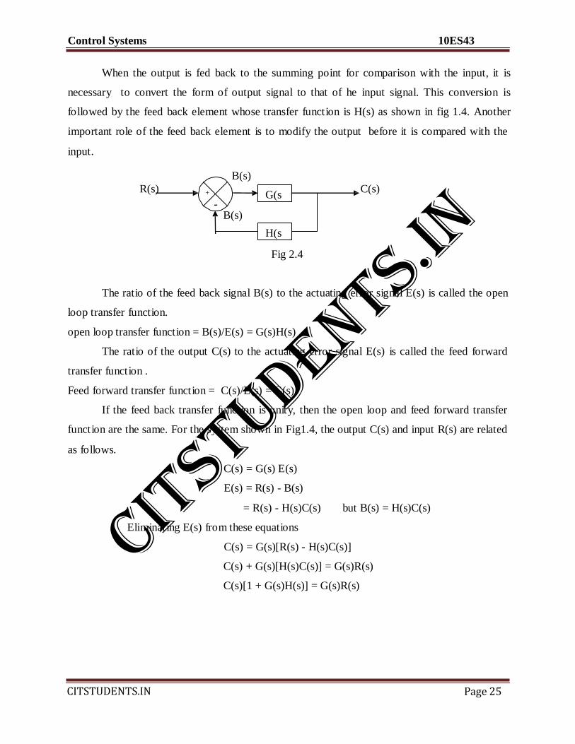
When the output is fed back to the summing point for comparison with the input, it is
necessary to convert the form of output signal to that of he input signal. This conversion is
followed by the feed back element whose transfer function is H(s) as shown in fig 1.4. Another
important role of the feed back element is to modify the output before it is compared with the
input.
R(s)
B(s)
+
- B(s)
G(s
H(s
Fig 2.4
C(s)
The ratio of the feed back signal B(s) to the actuating error signal E(s) is called the open
loop transfer function.
open loop transfer function = B(s)/E(s) = G(s)H(s)
The ratio of the output C(s) to the actuating error signal E(s) is called the feed forward
transfer function .
Feed forward transfer function = C(s)/E(s) = G(s)
If the feed back transfer function is unity, then the open loop and feed forward transfer
function are the same. For the system shown in Fig1.4, the output C(s) and input R(s) are related
as follows.
C(s) = G(s) E(s)
E(s) = R(s) - B(s)
= R(s) - H(s)C(s) but B(s) = H(s)C(s)
Eliminating E(s) from these equations
C(s) = G(s)[R(s) - H(s)C(s)]
C(s) + G(s)[H(s)C(s)] = G(s)R(s)
C(s)[1 + G(s)H(s)] = G(s)R(s)
CITSTUDENTS.IN

Control Systems 10ES43
CITSTUDENTS.IN
Page 26
C(s) G(s)
=
R(s) 1 + G(s)H(s)
C(s)/R(s) is called the closed loop transfer function.
The output of the closed loop system clearly depends on both the closed loop transfer
function and the nature of the input. If the feed back signal is positive, then
C(s) G(s)
=
R(s) 1 - G(s)H(s)
Closed loop system subjected to a disturbance
Fig2.5 shows a closed loop system subjected to a disturbance. When two inputs are present in
a linear system, each input can be treated independently of the other and the outputs
corresponding to each input alone can be added to give the complete output. The way in
which each input is introduced into the system is shown at the summing point by either a plus
or minus sign.
Disturbance
N(s)
R(s) +
-
G1(s)
+
+ G (s)
C(s)
H(s
Fig2.5
Fig2.5 closed loop system subjected to a disturbance.
Consider the system shown in fig 2.5. We assume that the system is at rest initially with
zero error. Calculate the response CN(s) to the disturbance only. Response is
CN(s) G2(s) =
R(s) 1 + G1(s)G2(s)H(s)
On the other hand, in considering the response to the reference input R(s), we may
assume that the disturbance is zero. Then the response CR(s) to the reference input R(s)is
CITSTUDENTS.IN

Control Systems 10ES43
CITSTUDENTS.IN
Page 27
CR(s) G1(s)G2(s)
= R(s) 1 + G1(s)G2(s)H(s).
The response C(s) due to the simultaneous application of the reference input R(s) and the
disturbance N(s) is given by
C(s) = CR(s) + CN(s)
G2(s)
C(s) = [G1(s)R(s) + N(s)] 1 + G1(s)G2(s)H(s)
Procedure for drawing block diagram :
To draw the block diagram for a system, first write the equation which describes the dynamic
behaviour of each components. Take the laplace transform of these equations, assuming zero
initial conditions and represent each laplace transformed equation individually in the form of
block. Finally assemble the elements into a complete block diagram.
As an example consider the Rc circuit shown in fig2.6 (a). The equations for the circuit
shown are
R
ei i eo
C
Fig. 2.6a
ei = iR + 1/c∫ idt -----------(1)
And
eo = 1/c∫ idt ---------(2)
Equation (1) becomes
ei = iR + eo
ei - eo
= i --------------(3) R
Laplace transforms of equations (2) & (3) are
CITSTUDENTS.IN

Control Systems 10ES43
CITSTUDENTS.IN
Page 28
Eo(s) = 1/CsI(s) -----------(4)
Ei(s) - Eo(s)
= I(s) -------- (5)
R
Equation (5) represents a summing operation and the corresponding diagram is shown in fig1.6
(b). Equation (4) represents the block as shown in fig2.6(c). Assembling these two elements, the
overall block diagram for the system shown in fig2.6(d) is obtained.
Ei(s) +
1/R
I(s) I(s) Eo(S)
1/C
_ Fig2.6(c)
Eo(s)
Eo(s) + I(s) Eo(s) 1/R 1/C
Fig2.6(b) _
Fig2.6(d)
SIGNAL FLOW GRAPHS
An alternate to block diagram is the signal flow graph due to S. J. Mason. A signal flow graph is
a diagram that represents a set of simultaneous linear algebraic equations. Each signal flow graph
consists of a network in which nodes are connected by directed branches. Each node represents a
system variable, and each branch acts as a signal multiplier. The signal flows in the direction
indicated by the arrow.
Definitions:
Node: A node is a point representing a variable or signal.
Branch: A branch is a directed line segment joining two nodes.
Transmittance: It is the gain between two nodes.
Input node: A node that has only outgoing branche(s). It is also, called as source and
corresponds to independent variable.
Output node: A node that has only incoming branches. This is also called as sink and
corresponds to dependent variable.
CITSTUDENTS.IN

Control Systems 10ES43
CITSTUDENTS.IN
Page 29
Mixed node: A node that has incoming and out going branches.
Path: A path is a traversal of connected branches in the direction of branch arrow.
Loop: A loop is a closed path.
Self loop: It is a feedback loop consisting of single branch.
Loop gain: The loop gain is the product of branch transmittances of the loop.
Nontouching loops: Loops that do not posses a common node.
Forward path: A path from source to sink without traversing an node more than once.
Feedback path: A path which originates and terminates at the same node.
Forward path gain: Product of branch transmittances of a forward path.
Properties of Signal Flow Graphs:
1) Signal flow applies only to linear systems.
2) The equations based on which a signal flow graph is drawn must be algebraic equations in the form of effects as a function of causes.
Nodes are used to represent variables. Normally the nodes are arranged left to right,
following a succession of causes and effects through the system.
3) Signals travel along the branches only in the direction described by the arrows of the branches.
4) The branch directing from node Xk to Xj represents dependence of the variable Xj on Xk
but not the reverse.
5) The signal traveling along the branch Xk and Xj is multiplied by branch gain akj and
signal akjXk is delivered at node Xj.
Guidelines to Construct the Signal Flow Graphs:
The signal flow graph of a system is constructed from its describing equations, or by direct
reference to block diagram of the system. Each variable of the block diagram becomes a node
and each block becomes a branch. The general procedure is
1) Arrange the input to output nodes from left to right.
2) Connect the nodes by appropriate branches.
3) If the desired output node has outgoing branches, add a dummy node and a unity gain branch.
4) Rearrange the nodes and/or loops in the graph to achieve pictorial clarity.
Signal Flow Graph Algebra
Addtion rule
CITSTUDENTS.IN

Control Systems 10ES43
CITSTUDENTS.IN
Page 30
The value of the variable designated by a node is equal to the sum of all signals entering the
node.
Transmission rule The value of the variable designated by a node is transmitted on every branch leaving the node.
Multiplication rule
A cascaded connection of n-1 branches with transmission functions can be replaced by a single branch with new transmission function equal to the product of the old ones.
Masons Gain Formula
The relationship between an input variable and an output variable of a signal flow graph is given
by the net gain between input and output nodes and is known as overall gain of the system.
Masons gain formula is used to obtain the over all gain (transfer function) of signal flow graphs.
Gain P is given by
1 P Pk k
k
Where, Pk is gain of kth
forward path,
∆ is determinant of graph
∆=1-(sum of all individual loop gains)+(sum of gain products of all possible combinations of
two nontouching loops – sum of gain products of all possible combination of three
nontouching loops) + ∙∙∙
∆k is cofactor of kth
forward path determinant of graph with loops touching kth
forward path. It is
obtained from ∆ by removing the loops touching the path Pk.
Example1
Draw the signal flow graph of the block diagram shown in Fig.2.7
H2
X1 X2 X3 X4 X5 X6 C R −
G1 G2 G3
−
H1
Figure 2.7 Multiple loop system
Choose the nodes to represent the variables say X1 .. X6 as shown in the block diagram. .
Connect the nodes with appropriate gain along the branch. The signal flow graph is shown in Fig. 2.7
CITSTUDENTS.IN

Control Systems 10ES43
CITSTUDENTS.IN
Page 31
R
-H2
R X1 X2 X3 C 1 1 G1 1 G2 G3 1
X4
X5 X6
H1
-1
Figure 1.8 Signal flow graph of the system shown in Fig. 2.7
Example 2.9
Draw the signal flow graph of the block diagram shown in Fig.2.9.
G1
X1 X2 C
− G2
G3
X3
−
G4
Figure 2.9 Block diagram feedback system
The nodal variables are X1, X2, X3.
The signal flow graph is shown in Fig. 2.10.
CITSTUDENTS.IN

Control Systems 10ES43
CITSTUDENTS.IN
Page 32
G1
R G2
X2 1
X3 1 C
X1
-G3
G4
Figure 2.10 Signal flow graph of example 2
Example 3 Draw the signal flow graph of the system of equations.
X 1 a11 X 1
X 2 a21 X 1
X 3 a31 X 1
a12 X 2
a22 X 2
a32 X 2
a13 X 3
a23 X 3
a33 X 3
b1u1
b2 u2
The variables are X1, X2, X3, u1 and u2 choose five nodes representing the variables.
Connect the various nodes choosing appropriate branch gain in accordance with the equations.
The signal flow graph is shown in Fig. 2.11.
a12
u2
a13
u1 b1
a11
b2
X2
a21
a32
a33
X1
X3
a22
a23
a31
Figure 2.11 Signal flow graph of example 2
CITSTUDENTS.IN

Control Systems 10ES43
CITSTUDENTS.IN
Page 33
c
L
Example 4
LRC net work is shown in Fig. 2.12. Draw its signal flow graph.
e(t)
−
R L
i(t) C
ec(t)
−
Figure 2.12 LRC network
The governing differential equations are
L di
Ri dt
or
di
1 idt
C
e t 1
L Ri ec
dt
dec
e t 2
C dt
i t 3
Taking Laplace transform of Eqn.1 and Eqn.2 and dividing Eqn.2 by L and Eqn.3 by C
sI s i 0
R I S
L
1 E s
L
1 E s 4
L
sEc s
ec 0 1
C I s 5
Eqn.4 and Eqn.5 are used to draw the signal flow graph shown in Fig.7.
i(0
+)
1
ec(0+)
1
L s R L
E(s)
s R 1
Cs
I(s)
-1
1
s
Ec(s)
L s R L
Figure 2.12 Signal flow graph of LRC system
CITSTUDENTS.IN

Control Systems 10ES43
CITSTUDENTS.IN
Page 34
SIGNAL FLOW GRAPHS
The relationship between an input variable and an output variable of a signal flow graph is given
by the net gain between input and output nodes and is known as overall gain of the system.
Masons gain formula is used to obtain the over all gain (transfer function) of signal flow graphs.
Masons Gain Formula
Gain P is given by
1 P Pk k
k
Where, Pk is gain of kth
forward path,
∆ is determinant of graph
∆=1-(sum of all individual loop gains)+(sum of gain products of all possible combinations of
two nontouching loops – sum of gain products of all possible combination of three
nontouching loops) + ∙∙∙
∆k is cofactor of kth
forward path determinant of graph with loops touching kth
forward path. It is
obtained from ∆ by removing the loops touching the path Pk.
Example 1 Obtain the transfer function of C/R of the system whose signal flow graph is shown in Fig. 2.13
G1
R G2 1 1 C
-G3
G4
Figure 2.13 Signal flow graph of example 1
There are two forward paths:
Gain of path 1 : P1=G1
Gain of path 2 : P2=G2
There are four loops with loop gains:
L1=-G1G3, L2=G1G4, L3= -G2G3, L4= G2G4
CITSTUDENTS.IN

Control Systems 10ES43
CITSTUDENTS.IN
Page 35
There are no non-touching loops.
∆ = 1+G1G3-G1G4+G2G3-G2G4
Forward paths 1 and 2 touch all the loops. Therefore, ∆1= 1, ∆2= 1
The transfer function T = C s R s
P1 1 P2 2
1 G1G3
G1
G1G4
G2
G2 G3
G2 G4
Example 2
Obtain the transfer function of C(s)/R(s) of the system whose signal flow graph is shown in
Fig.2.14.
R(s) 1 1
-H2
G1 G2 G3
1 C(s)
H1
-1
Figure 2.14 Signal flow graph of example 2
There is one forward path, whose gain is: P1=G1G2G3
There are three loops with loop gains:
L1=-G1G2H1, L2=G2G3H2, L3= -G1G2G3
There are no non-touching loops.
∆ = 1-G1G2H1+G2G3H2+G1G2G3
Forward path 1 touches all the loops. Therefore, ∆1= 1.
The transfer function T = C s R s
P1 1
1 G1G2 H1
G1G2 G3
G1G3 H 2
G1G2 G3
Example 3
Obtain the transfer function of C(s)/R(s) of the system whose sig nal flow graph is shown in Fig.2.15.
CITSTUDENTS.IN

Control Systems 10ES43
CITSTUDENTS.IN
Page 36
2
G6 G7
R(s)
G1 G
G3 G4
G5 1
C(s)
X1 X2 X3 X4 X5
-H1
-H2
Figure 2.15 Signal flow graph of example 3
There are three forward paths.
The gain of the forward path are: P1=G1G2G3G4G5
P2=G1G6G4G5
P3= G1G2G7
There are four loops with loop gains:
L1=-G4H1, L2=-G2G7H2, L3= -G6G4G5H2 , L4=-G2G3G4G5H2
There is one combination of Loops L1 and L2 which are nontouching with loop gain product L1L2=G2G7H2G4H1
∆ = 1+G4H1+G2G7H2+G6G4G5H2+G2G3G4G5H2+ G2G7H2G4H1
Forward path 1 and 2 touch all the four loops. Therefore ∆1= 1, ∆2= 1. Forward path 3 is not in touch with loop1. Hence, ∆3= 1+G4H1.
The transfer function T =
C s P1 1 P2 2 P3 3 G1G2 G3G4 G5 G1G4 G5G6 G1G2 G7 1 G4 H1
R s 1 G4 H
1 G
2 G
7 H
2 G
6 G
4 G
5 H
2 G
2 G
3G
4 G
5 H
2 G2 G4 G7 H1 H
2
Example 4
CITSTUDENTS.IN

Control Systems 10ES43
CITSTUDENTS.IN
Page 37
X
Find the gains X 6 ,
X 5 , X 3
for the signal flow graph shown in Fig.2.16. X 1 X 2 X 1
b
X1 a c d
-h
e X5 f X6
X2 X3 X4
-g
-i
Figure 2.16 Signal flow graph of MIMO system
X Case 1: 6
X 1
There are two forward paths.
The gain of the forward path are: P1=acdef
P2=abef There are four loops with loop gains:
L1=-cg, L2=-eh, L3= -cdei, L4=-bei There is one combination of Loops L1 and L2 which are nontouching with loop gain product L1L2=cgeh ∆ = 1+cg+eh+cdei+bei+cgeh
Forward path 1 and 2 touch all the four loops. Therefore ∆1= 1, ∆2= 1.
X 6
P1 1
P2 2
cdef abef The transfer function T =
1
1 cg
eh cdei
bei
cgeh
X Case 2:
5
X 2
The modified signal flow graph for case 2 is shown in Fig.2.17.
CITSTUDENTS.IN

Control Systems 10ES43
CITSTUDENTS.IN
Page 38
X
X2 1
b
c d
X2 X3
-h
e X5
1 X5
X4
-g
-i
Figure 2.17 Signal flow graph of example 4 case 2
The transfer function can directly manipulated from case 1 as branches a and f are removed
which do not form the loops. Hence,
X 5
P1 1
P2 2
cde be The transfer function T=
2
1 cg
eh cdei
bei
cgeh
X
Case 3: 3
X 1
The signal flow graph is redrawn to obtain the clarity of the funct ional relation as shown in
Fig.2.18. -h
X1 a X2 b e
c
X5 f
1 X3
X4 X3
-i d
-g
Figure 2.18 Signal flow graph of example 4 case 3
There are two forward paths.
The gain of the forward path are: P1=abcd
P2=ac
CITSTUDENTS.IN

Control Systems 10ES43
CITSTUDENTS.IN
Page 39
X
1
There are five loops with loop gains:
L1=-eh, L2=-cg, L3= -bei, L4=edf, L5=-befg
There is one combination of Loops L1 and L2 which are nontouching with loop gain product L1L2=ehcg ∆ = 1+eh+cg+bei+efd+befg+ehcg
Forward path 1 touches all the five loops. Therefore ∆1= 1.
Forward path 2 does not touch loop L1. Hence, ∆2= 1+ eh
X 3
P1 1
P2 2
abef ac 1 eh The transfer function T =
1
1 eh cg
bei
efd
befg
ehcg
Example 5
For the system represented by the following equations find the transfer function X(s)/U(s) using
signal flow graph technique.
X X 1 3u
X 1 a1 X 1 X 2 2 u
X 2 a2 X 1 1u
Taking Laplace transform with zero initial conditions
X s X 1 s 3U s
sX 1 s a1 X 1 s X 2 s 2U s
sX 2 s a2 X 1 s 1U s
Rearrange the above equation
X s X 1
X s
s
a1 X
3U s
s 1
X s
2 U s
1
X 2 s
s 1
a2 X s s
s 2
s
1 U s s
The signal flow graph is shown in Fig.2.19. CIT
STUDENTS.IN

Control Systems 10ES43
CITSTUDENTS.IN
Page 40
β
s 2
2
1
s
a1
2 a 2
s X1 s
s X X
X2
U β1
s 1
3
Figure 2.19 Signal flow grapgh of example 5
There are three forward paths.
The gain of the forward path are: P1= 3
P2= 1/ s2
P3= 2/ s
There are two loops with loop gains:
L a1
1 s
L a2
2 s
2
L1=-eh, L2=-cg, L3= -bei, L4=edf, L5=-befg
There are no combination two Loops which are nontouching.
1 a1 a2
s s 2
Forward path 1 does not touch loops L1 and L2. Therefore
1 a1 a2
1 s s
2
Forward path 2 path 3 touch the two loops. Hence, ∆2= 1, ∆2= 1.
X
3 P
1 1 P
2 2 P
3 3
3 a
1 s a
2
2 s
1
The transfer function T = X 1
s a1 s a
2
CITSTUDENTS.IN

Control Systems 10ES43
CITSTUDENTS.IN
Page 41
R
Recommended Questions:
1. Define block diagram & depict the block diagram of closed loop system.
2. Write the procedure to draw the block diagram.
3. Define signal flow graph and its parameters
4. Explain briefly Mason‘s Gain formula
5. Draw the signal flow graph of the block diagram shown in Fig below.
H2
X1 X2 X3 X4 X5 X6 C R −
G1 G2 G3
−
H1
6. Draw the signal flow graph of the block diagram shown in Fig below
G1
X1 X2 C
− G2
G3
X3
−
G4
7. For the LRC net work is shown in Fig Draw its signal flow graph.
CITSTUDENTS.IN
Control Systems 10ES43
CITSTUDENTS.IN
Page 42
2
e(t)
−
R L
i(t) C
ec(t)
−
Figur
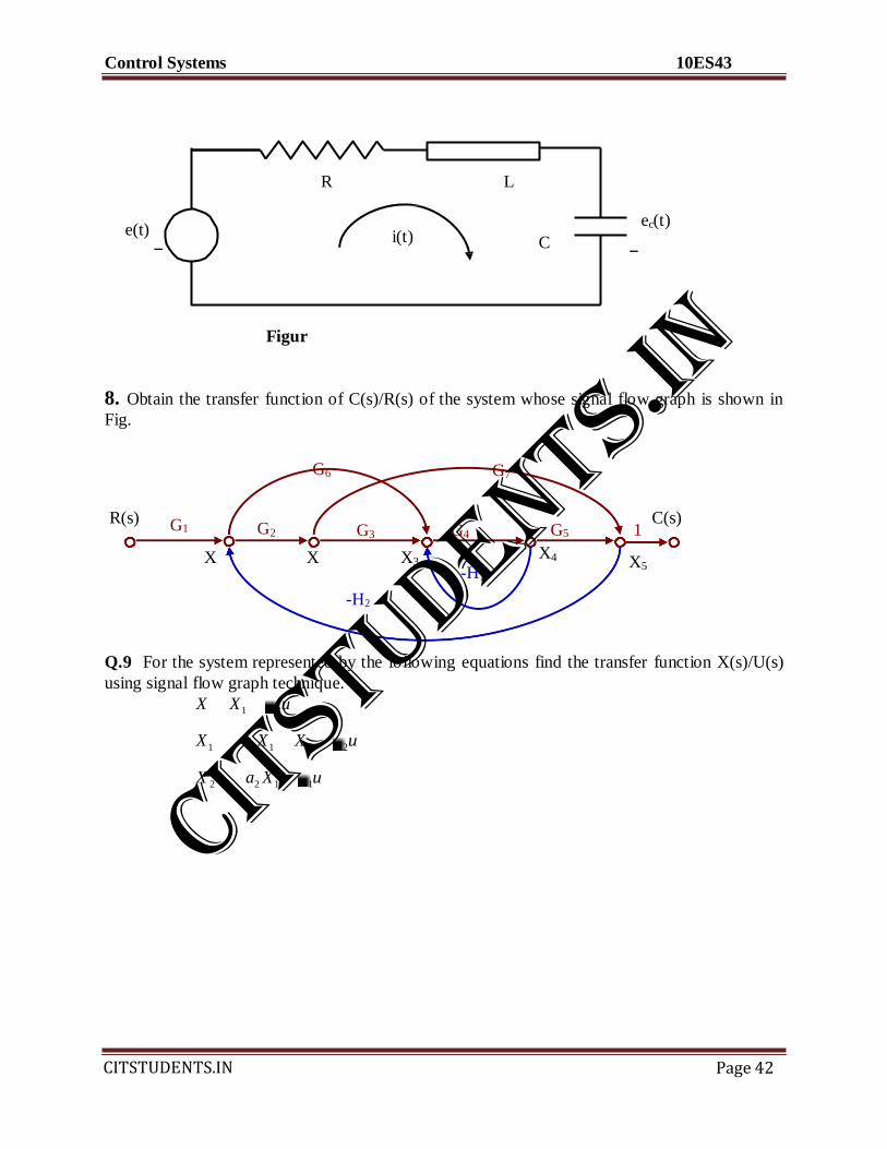
8. Obtain the transfer function of C(s)/R(s) of the system whose signal flow graph is shown in
Fig.
G6 G7
R(s) G1 G
G3 G4
G5 1 C(s)
X X X3 X4 X5
-H1
-H2
Q.9 For the system represented by the following equations find the transfer function X(s)/U(s)
using signal flow graph technique.
X X1 3u
X1 a1 X1 X 2 2u
X 2 a2 X1 1u
CITSTUDENTS.IN

Control Systems 10ES43
CITSTUDENTS.IN
Page 43
UNIT- 3
Time response analysis of control systems:
Introduction:
Time is used as an independent variable in most of the control systems. It is important to
analyse the response given by the system for the applied excitation, which is function of time.
Analysis of response means to see the variation of out put with respect to time. The output
behavior with respect to time should be within these specified limits to have satisfactory
performance of the systems. The stability analysis lies in the time response analysis that is when
the system is stable out put is finite
The system stability, system accuracy and complete evaluation is based on the time
response analysis on corresponding results.
DEFINITION AND CLASSIFICATION OF TIME RESPONSE
Time Response:
The response given by the system which is function of the time, to the applied excitation is called time response of a control system.
Practically, output of the system takes some finite time to reach to its final value.
This time varies from system to system and is dependent on different factors.
The factors like friction mass or inertia of moving elements some nonlinearities present etc. Example: Measuring instruments like Voltmeter, Ammeter.
Classification:
The time response of a control system is divided into two parts.
1 Transient response ct(t) 2 Steady state response css(t)
. . . c(t)=ct(t) +cSS(t)
Where c(t)= Time Response
Total Response=Zero State Response +Zero Input Response
Transient Response:
It is defined as the part of the response that goes to zero as time becomes very large. i,e,
Lim ct(t)=0 t
A system in which the transient response do not decay as time progresses is an Unstable
system.
CITSTUDENTS.IN

Control Systems 10ES43
CITSTUDENTS.IN
Page 44
C(t)
Step
Ct(t) Css(t)
ess
= study state
error
O Time
Transient time Study state
Time
The transient response may be experimental
or oscillatory in nature.
2. Steady State Response:
It is defined the part of the response which remains after complete transient response
vanishes from the system output.
. i,e, Lim ct(t)=css(t) t
The time domain analysis essentially involves the evaluation of the transient and
Steady state response of the control system.
Standard Test Input Signals
For the analysis point of view, the signals, which are most commonly used as refere nce
inputs, are defined as standard test inputs.
The performance of a system can be evaluated with respect to these test signals.
Based on the information obtained the design of control system is carried out.
The commonly used test signals are
1. Step Input signals. 2. Ramp Input Signals.
3. Parabolic Input Signals.
4. Impulse input signal.
Details of standard test signals
1. Step input signal (position function)
It is the sudden application of the input at a specified time as usual in the figure or
instant any us change in the reference input
Example :-
a. If the input is an angular position of a mechanical shaft a step input represent
the sudden rotation of a shaft.
b. Switching on a constant voltage in an electrical circuit.
CITSTUDENTS.IN

Control Systems 10ES43
CITSTUDENTS.IN
Page 45
R(S) = A = 1
S2
S2
LT f
c. Sudden opening or closing a valve.
r(t)
A
O t
When, A = 1, r(t) = u(t) = 1
The step is a signal who‘s value changes from 1 value (usually 0) to another level A in
Zero time.
In the Laplace Transform form R(s) = A / S
Mathematically r(t) = u(t) = 1 for t > 0
= 0 for t < 0
2. Ramp Input Signal (Velocity Functions):
It is constant rate of change in input that is gradual application of input as shown
in fig (2 b). r(t)
Ex:- Altitude Control
of a Missile
Slope = A
t
O
time.
The ramp is a signal, which starts at a value of zero and increases linearly with
Mathematically r (t) = At for t ≥ 0
= 0 for t≤ 0.
In LT form R(S) = A
S2
If A=1, it is called Unit Ramp Input
Mathematically
r(t) = t u(t)
{
In =
orm t for t ≥ 0 0 for t ≤ 0
CITSTUDENTS.IN

Control Systems 10ES43
CITSTUDENTS.IN
Page 46
1 3
3. Parabolic Input Signal (Acceleration function):
The input which is one degree faster than a ramp type of input as shown in fig (2 c) or
it is an integral of a ramp .
Mathematically a parabolic signal of magnitude
A is given by r(t) = A t
2 u(t)
2
Slope = At
r(t) At2
for t ≥ 0
= 2
0 for t ≤ 0 t
In LT form R(S) = A
S3
If A = 1, a unit parabolic function is defined as r(t) = t2
u(t)
2
ie., r(t)
{
In LT for R(S) =
S =
4. Impulse Input Signal :
t
2 for t ≥ 0
2
0 for t ≤ 0
It is the input applied instantaneously (for short duration of time ) of very high amplitude
as shown in fig 2(d)
Eg: Sudden shocks i e, HV due lightening or short circuit.
It is the pulse whose magnitude is infinite while its width tends to zero.
r(t)
ie., t 0 (zero) applied
momentarily
A
O t ∆ t 0
Area of impulse = Its magnitude
If area is unity, it is called Unit Impulse Input denoted as (t)
Mathematically it can be expressed as
r(t) = A for t = 0
CITSTUDENTS.IN

Control Systems 10ES43
CITSTUDENTS.IN
Page 47
= 0 for t ≠ 0
In LT form R(S) = 1 if A = 1
Standard test Input Signals and its Laplace Transforms.
r(t) R(S)
Unit Step 1/S
Unit ramp 1/S2
Unit Parabolic 1/S3
Unit Impulse 1
First order system:-
The 1st
order system is represent by the differential Eq:- a1dc(t )+aoc (t) = bor(t)------ (1)
dt
Where, e (t) = out put , r(t) = input, a0, a1 & b0 are constants.
Dividing Eq:- (1) by a0, then a1. d c(t ) + c(t) = bo.r (t)
a0 dt ao
T . d c(t ) + c(t) = Kr (t) ---------------------- (2)
dt
Where, T=time const, has the dimensions of time = a1 & K= static sensitivity = b0
a0 a0
Taking for L.T. for the above Eq:- [ TS+1] C(S) = K.R(S)
T.F. of a 1st
order system is ; G(S) = C(S ) = K .
R(S) 1+TS
If K=1, Then G(S) = 1 .
1+TS
[ It‘s a dimensionless T.F.]
……I
This system represent RC ckt. A simplified bloc diagram is as shown.;
R(S)+ 1 C(S)
TS
-
CITSTUDENTS.IN

Control Systems 10ES43
CITSTUDENTS.IN
Page 48
Unit step response of 1st
order system:-
Let a unit step i\p u(t) be applied to a 1st
order system,
Then, r (t)=u (t) & R(S) = 1 . ---------------(1)
S W.K.T. C(S)
= G(S). R(S)
C(S) = 1 . 1 . = 1 . T . ----------------- (2)
1+TS S S TS+1
Taking inverse L.T. for the above Eq:-
then, C(t)=u (t) – e –t/T
; t.>0.------------- (3) slope = 1 . T
At t=T, then the value of c(t)= 1- e –1
= 0.632. c (t)
The smaller the time const. T. the
faster the system response.
The slope of the tangent line at at t= 0 is 1/T.
Since dc = 1 .e -t/T
= 1 . at t .=0. ------------- (4)
dt T T
0.632
1 – e
–t/T
t
T
From Eq:- (4) , We see that the slope of the response curve c(t) decreases monotonically from 1
. at t=0 to zero. At t=
T
Second order system:-
The 2nd
order system is defined as,
a2 d2
c(t) + a1 dc(t) + a0 c(t) = b0 .r(t)-----------------(1)
dt2
dt
Where c(t) = o/p & r(t) = I/p
-- ing (1) by a0,
a2 d
2 c(t) + a1 . dc (t) + c(t) = b0 . r(t).
a0 dt2
a0 dt a0
a2 d
2 c(t) + 2a1 . a2 . dc (t) + c(t) = b0 . r(t).
a0 dt2
2 a0 a0 . a2 dt a0
3) The open loop T.F. of a unity feed back system is given by G(S) = K . where,
S(1+ST)
CITSTUDENTS.IN

Control Systems 10ES43
CITSTUDENTS.IN
Page 49
T&K are constants having + Ve values.By what factor (1) the amplitude gain be reduced so
that (a) The peak overshoot of unity step response of the system is reduced from 75% to 25%
(b) The damping ratio increases from 0.1 to 0.6.
Solution: G(S) = K .
S(1+ST)
Let the value of damping ratio is, when peak overshoot is 75% & when peak
overshoot is 25%
Mp = .
e 1- 2
ln 0. 75 = . 0.0916 = .
1- 2
1- 2
1 = 0.091 (0.0084) (1- 2) =
2
2 = 0.4037 (1.0084 2) = 0.0084
= 0.091
k .
S + S2T .
w.k.t. T.F. = G(S) = 1 + K . = K .
1+ G(S) . H(S) S + S2T S + S
2T+K
T.F. = K / T .
S2
+ S + K .
T T
Comparing with std Eq :-
Wn = K . , 2 Wn = 1 .
T T
Let the value of K = K1 When = 1 & K = K2 When = 2.
Since 2 Wn = 1 . , = 1 . = 1 .
T 2TWn 2 KT 1 .
1 . = 2 K1T = K2 .
2 1 K1
2 K2T
0.091 = K2 . K2 . = 0.0508
0.4037 K1 K1
CITSTUDENTS.IN

Control Systems 10ES43
CITSTUDENTS.IN
Page 50
K2 = 0.0508 K1
a) The amplitude K has to be reduced by a factor = 1 . = 20
0.0508
b) Let = 0.1 Where gain is K1 and
= 0.6 Where gain is K2
0.1 = K2 . K2 . = 0.027 K2 = 0.027 K1
0.6 K1 K1
The amplitude gain should be reduced by 1 . = 36
0.027
4) Find all the time domain specification for a unit y feed back control system whose open loop
T.F. is given by
G(S) = 25 .
S(S+6)
Solution:
25 .
G(S) = 25 . G(S) . = S(S+6) .
S(S+6) 1 + G(S) .H(S) 1 + 25 .
S(S+6)
= 25 .
S2 + ( 6S+25 )
W
2n = 25 , Wn = 5, 2 Wn = 6 = 6 . = 0.6
2 x 5
Wd = Wn 1- 2
= 5 1- (0.6)2
= 4
tr = - , = tan-1
Wd = Wn = 0.6 x 5 = 3
Wd
= tan-1
( 4/3 ) = 0.927 rad.
tp = . = 3.14 = 0.785 sec.
Wd 4
MP = . = 0.6 . x3.4 = 9.5%
e 1- 2
e 1- 0.62
ts = 4 . for 2% = 4 . = 1.3 ………3sec.
Wn 0.6 x 5
CITSTUDENTS.IN

Control Systems 10ES43
CITSTUDENTS.IN
Page 51
5) The closed loop T.F. of a unity feed back control system is given by
C(S) = 5 .
R(S) S2 + 4S +5
Determine (1) Damping ratio (2) Natural
undamped response frequency Wn. (3) Percent
peak over shoot Mp (4) Expression for error
resoponse.
Solution:
C(S) = 5 . , Wn2 = 5 Wn = 5 = 2.236
R(S) S2 + 4S +5
2 Wn = 4 = 4 . = 0.894. Wd = 1.0018
2 x 2.236
MP = . = 0.894 . X 3.14 = 0.19%
e 1- 2
e 1-(0.894)2
W. K.T. C(t) = e- Wnt
Cos Wdtr + . sin wdtr
1- 2
= e-0.894x2.236t
Cos 1.0018t + 0.894 . sin 1.0018t
1-(0.894)2
6) A servo mechanism is represent by the Eq:-
d2
+ 10 d = 150E , E = R- is the actuating signal calculate the
dt2
dt value of damping ratio, undamped and damped frequency of ascillation.
Soutions:- d
2 + 10 d = 15 ( r - ) , = 150r – 150 .
dt2
dt
Taking L.T., [S2
+ 10S + 150] (S) = 150 R (S).
(S) = 150 .
R(S) S2
+ 10S + 15O
Wn2
= 150 Wn = 12.25. ………………………….rad sec .1
2 Wn = 10 = 10 . = 0.408.
2 x 12.25
CITSTUDENTS.IN

Control Systems 10ES43
CITSTUDENTS.IN
Page 52
Wd = Wn 1 - 2 = 12.25 1- (0.408)2 = 11.18. rad 1sec.
7) Fig shows a mechanical system and the response when 10N of force is applied to the system.
Determine the values of M, F, K,.
K x(t)inmt
f(t) 0.00193
The T.F. of the mechanical system is , 0.02
X(S) = 1 . M
F(S) MS2
+ FS = K
f(t) = Md2X + F dX + KX
F x dt2
dt
F(S) = (MS2
+ FS + K) x (S)
1 2 3 4 5
Given :- F(S) = 10
S.
X(S) = 10 .
S(MS2
+ FS + K)
SX (S) = 10 .
MS2
+ FS + K
The steady state value of X is By applying final value theorem,
lt. SX(S) = 10 . = 10 = 0.02 ( Given from Fig.)
S O M(0) + F (0) + K K. ( K = 500.)
MP = 0.00193 = 0.0965 = 9.62%
0.02
MP = e . ln 0.0965 = .
1 - 2
1 - 2
0.744 = . 0.5539 = 2
.
1 - 2
1 - 2
0.5539 – 0.5539 2
= 2
= 0.597 = 0.6
tp = = .
Wd Wn 1 – 2
3 = . Wn = 1.31…… rad / Sec.
CITSTUDENTS.IN

Control Systems 10ES43
CITSTUDENTS.IN
Page 53
Wn 1 – (0.6)2
Sx(S) = 10/ M .
(S2
+ F S + K )
M M
Comparing with the std. 2nd
order Eq :-, then,
Wn2
= K
Wn = K (1.31)2
= 500 .
M = 291.36 kg.
M M M
F = 2 Wn F = 2 x 0.6 x 291 x 1.31
M F = 458.7 N/M/ Sec.
8) Measurements conducted on sever me mechanism show the system response to be c(t) =
1+0.2e-60t
– 1.2e-10t
, When subjected to a unit step i/p. Obtain the expression for closed
loop T.F the damping ratio and undamped natural frequency of oscillation .
Solution: C(t) = 1+0.2e
-60t –1.2e
-10t
Taking L.T., C(S) = 1 . + 0.2 . – 1.2 .
S S+60 S+10
C(S) . = 600 / S .
S2
+ 70S + + 600
Given that :- Unit step i/p r(t) = 1 R(S) = 1 .
C(S) . = 600 / S .
R(S) S2
+ 70S + + 600
Comparing, Wn2
= 600, 24.4 …..rad / Sec
70, = 70 . = 1.428
2 x 24.4
2 Wn =
10) A feed back system employing o/p damping is as shown in fig.
1) Find the value of K1 & K2 so that closed loop system resembles a 2nd
order system with = 0.5 & frequency of damped oscillation 9.5 rad / Sec.
CITSTUDENTS.IN

Control Systems 10ES43
CITSTUDENTS.IN
Page 54
2) With the above value of K1 & K2 find the % overshoot when i/p is step i/p
3) What is the % overshoot when i/p is step i/p, the settling time for 2% tolerance?
K1 1 . S(1+S)
R + C
K2S
C . = K1 .
R S2
+ ( 1 + K2 ) S + K1
Wn2
= K1 Wn = K1
2 Wn = 1 + K2 = 1 + K2
2 K1
Wd = Wn 1 - 2
Wn = 9.5 . 10.96 rad/Sec
1 – 0.52
K1 = (10.96)2
= 120.34
2 Wn = 1 + K2 , K2 = 9.97
MP = . = 16.3%
e 1 - 2
ts = 4 . = 4 . = 0.729 sec
Wn 0.5 x 10.97
Steady state Error :-
Steady state errors constitute an extremely important aspect of system
performance. The state error is a measure of system accuracy. These errors arise from the nature
of i/p‘s type of system and from non-linearties of the system components. The steady state
performance of a stable control system is generally judged by its steady state error to step, ramp
and parabolic i/p.
CITSTUDENTS.IN

Control Systems 10ES43
CITSTUDENTS.IN
Page 55
Consider the system shown in the fig.
G(S)
R(S) E(S) C(S)
H(S)
C(S) = G(S) . …………………………(1)
R(S) 1+G(S) . H(S)
The closed loop T.F is given by (1). The T.F. b/w the actuating error signal e(t) and the
i/p signal r(t) is,
E(S) = R(S) – C(S) H(S) = 1 – C(S) . H(S)
R(S) R(S) R(S)
= 1 – G(S) . H(S) . = 1 + G(S) . H(S) – G(S)H(S)
1 + G(S) . H(S) 1+G(S) . H(S)
= 1 .
1 + G(S) . H(S)
Where e(t) = Difference b/w the i/p signal and the feed back signal
E(S) = 1 . .R(S) ……………………….(1)
1 + G(S) . H(S)
The steady state error ess may be found by the use of final value theorem
and is as follows;
ess = lt e(t) = lt SE(S)
t S O
Substituting (1), ess = lt S.R(S) . ……………….(2)
S O 1+G(S) . H(S)
Eq :- (2) Shows that the steady state error depends upon the i/p R(S) and the forward T.F.
G(S) and loop T.F G(S) . H(S).
CITSTUDENTS.IN

Control Systems 10ES43
CITSTUDENTS.IN
Page 56
The expression for steady state errors for various types of standard test signals are
derived below; 1) Steady state error due to step i/p or position error constant (Kp):-
The steady state error for the step i/p is
I/P r(t) = u(t). Taking L.T., R(S) = 1/S.
From Eq:- (2), ess = lt S. R(s) . = 1 .
S O 1 +G(S). H.S 1 + lt G(S). H(S)
S O
lt G(S) . H(S) = Kp
(S O )
Where Kp = proportional error constant or position error const.
ess = 1 .
1 + Kp
(1 + Kp) ess = 1 Kp = 1 - ess
ess
Note :- ess = R . for non-unit step i/p
1 + Kp
2) Steady state error due to ramp i/p or static velocity error co-efficient (Kv) :-
The ess of the system with a unit ramp i/p or unit velocity i/p is given by,
r ( t) = t. u(t) , Taking L -T, R(S) = 1/S2
Substituting this to ess Eq:-
ess = lt S . . 1 . = lt 1 .
S O 1 + G(S) . H(s) S2
S O S +S G(S) H(s)S
lt = SG(S) . H(S) = Kv = velocity co-efficient then
S O
ess = lt 1 . ess = 1 .
S O S + Kv Kv
Velocity error is not an error in velocity , but it is an error in position error due to a ramp
i/p
3) Steady state error due to parabolic i/p or static acceleration co-efficient (Ka) :-
The steady state actuating error of the system with a unit parabolic i/p (acceleration i/p)
which is defined by r(t) + 1 . t2
Taking L.T. R(S)= 1 .
2 S3
CITSTUDENTS.IN

Control Systems 10ES43
CITSTUDENTS.IN
Page 57
S
.
ess = lt S . 1 . lt 1 .
S O 1 + G(S) . H(S) S3
S O S2
+ S2
G(S) . H(S)
lt 2 G(S) . H(S) = Ka.
S O
ess = lt 1 . = 1 .
S O S2
+ Ka Ka
Note :- ess = R . for non unit parabolic.
Ka
Types of feed back control system :-
The open loop T.F. of a unity feed back system can be written in two std, forms;
1) Time constant form and 2) Pole Zero form,
G(S) = K(TaS +1) (TbS +1)…………………..
Sn(T1 S+1) (T2S + 1)……………….
Where K = open loop gain.
Above Eq:- involves the term Sn
in denominator which corresponds to no, of
integrations in the system. A system is called Type O, Type1, Type2,……….. if n = 0, 1,
2, ………….. Respectively. The Type no., determines the value of error co-efficients. As the type no., is increased, accuracy is improved; however increasing the type no.,
aggregates the stability error. A term in the denominator represents the poles at the origin
in complex S plane. Hence Index n denotes the multiplicity of the poles at the origin.
The steady state errors co-efficient for a given type have definite values. This is
illustration as follows.
1) Type – O system :- If, n = 0, the system is called type – 0, system. The
steady state error are as follows;
Let, G(S) = K . [ . .
H(s) = 1]
S + 1
ess (Position) = 1 . = 1 . = 1 .
1 + G(O) . H(O) 1 + K 1 + Kp
. .
K
= lt G(S) . H(S) = lt K . = K
. p
S O S O S + 1
ess (Velocity) = 1 . = 1 . =
Kv O
CITSTUDENTS.IN

Control Systems 10ES43
CITSTUDENTS.IN
Page 58
Kv = lt G(S) . H(S) = lt S K . = O.
S O S O S + 1
ess (acceleration) = 1 . = 1 . =
Ka O
Ka = lt S2
G(S) . H(S) = lt S2
K . = O.
S O S O S + 1
2) Type 1 –System :- If, n = 1, the ess to various std, i/p, G(S) = K .
S (S + 1)
ess (Position) = 1 . = O
1 +
Kp = lt G(S) . H(S) = lt K . =
S O S O S( S + 1)
Kv = lt S K . = K
S O S(S+1)
ess (Velocity) = 1 . K
ess (acceleration) = 1 . = 1 . =
O O
Ka = lt S2
K . = O.
S O S (S + 1)
3) Type 2 –System :- If, n = 2, the ess to various std, i/p, are , G(S) = K .
S2
(S + 1)
Kp = lt K . = S
O S2
(S + 1)
. .
. ess (Position) = 1 . = O
Kv = lt S K . =
S O S2
(S + 1)
. .
. ess (Velocity) = 1 . = O
CITSTUDENTS.IN

Control Systems 10ES43
CITSTUDENTS.IN
Page 59
Ka = lt S2 K . = K.
S O S2
(S + 1)
. .
. ess (acceleration) = 1 . K
3) Type 3 –System :- Gives Kp = Kv = Ka = & ess = O.
(Onwards)
The error co-efficient Kp, Kv, & Ka describes the ability of the system to eliminate the steady
state error therefore they are indicative of steady state performance. It is generally described to
increase the error co-efficient while maintaining the transient response within an acceptable
limit.
PROBLEMS;
1. The unit step response of a system is given by
C (t) = 5/2 +5t – 5/2 e-2t
. Find the T. F of the system.
T/P = r(t) = U (t). Taking L.T, R(s) = 1/S.
Response C(t) = 5/2+5t-5/2 e-2t
1 + 2 - 1
S S2
S+2
Taking
L.T, C(s)
= 5 1 + 5 1 5 1 = 5
2 S S2
2 (S+2) 2
S
2 = 5
2
= 10 (S+1)
S2 (S+2)
S2+2S+2S+4—
C(s) = 5 S(S+2)+2(S+2)-
2 S2(
S+2)
T.F = C (S) = 10 (S+1) S = 10 (S+1)
R (S) S2(S+2) S(S+2)
2. The open loop T F of a unity food back system is G(s) = 100
S (S+10)
CITSTUDENTS.IN

Control Systems 10ES43
CITSTUDENTS.IN
Page 60
Find the static error constant and the steady state error of the system when subjected to an i/p
given by the polynomial
R(t) = Po + p1t + P2 t2
2
G(s) = 100 position error co-efficient
S (S+10)
S 0 S 0 S (S+10)
KP = lt G(s) = lt 100 =
Similarly KV = lt SG(s) = lt 100 x s = 100 = 10
S 0 S 0 S (S+10)
lt 100 x s2 = 0
S 0 S 0 S (S+10)
Ka = lt S2 G(S)
Given :- r(t) = Po+P1t +P2 t2
2
Therefore steady state error ess
R1 R2 R3
+ +
1+Kp Kv Ka
ess
R1 R2
R3+
+ =
P0 P1
P2
+ +
Ess = 0+0.1 P1 + =
3. Determine the error co-efficeint and static error for G(s) = 1
And H(s) = (S+2) S(S+1) (S+10)
CITSTUDENTS.IN

Control Systems 10ES43
CITSTUDENTS.IN
Page 61
(
+2)
The error constants for a non unity feed back system is as follows
Kp = lt G(S) H(S) =
lt S
G(S).H(S) =
(0+2)
=
0(0+1) (0+10)
S(S+1) (S+10)
Kv = lt G(S) H(S) =
lt
(0+2)
0(0+1) (0+10)
= 1/5 = 0.2
Ka = 0
Static Error:-
Steady state error for unit step i/p = 0
Unit ramp i/p
1 1
= = 5
Kv 0.2
Unit parabolic i/p = 1/0 =
4. A feed back C.S is described as G(S) = 50
H(S)=1/s.For unit step i/p,cal steady state error
constant and errors. S (S+2) (S+5)
Kp = lt G(S) H(S) =
lt
50
=
S2
(S+2) (S+5)
Kv = lt G(S) H(S) =
lt
50 x S
=
S2
(S+2) (S+5)
Ka = lt G(S) H(S) = lt
S 0 S 0
S2 x 50 50
= = 5
S2
(S+2) (S+5) 10
CITSTUDENTS.IN

Control Systems 10ES43
CITSTUDENTS.IN
Page 62
0)
The steady state error Ess = lt S. 1/S
S 0 1+50 Lt S
2 (S+2) (S+5)
= 0/50 = 0
S 0 S2
(S+2) (S+5) + 50
K
5. A certain feed back C.S is described by following C.S G(S)
=
H(S) = 1
S2
(S+20) (S+30)
Determine steady state error co-efficient and also determine the value of K to limit the steady to
10 units due to i/p r(t) = 1 + 10 + t 20/2 t2.
Kp = lt G(S) H(S) =
lt
50
=
S2
(S+20) (S+30)
Kv = lt S K
S 0 S2
(S+20) (S+30) =
Ka = lt S2
K
S 0 S2
(S+20) (S+3
K
600
Steady state error:-
Error due to unit step i/p
Error due o r(t) ramp i/p
1 1
+ = 0
1+Kp 1+
10 10
+ = 0
Kv
CITSTUDENTS.IN

Control Systems 10ES43
CITSTUDENTS.IN
Page 63
=
…
Error due to para i/p,
,
20 40
=
Ka 2Ka
20 x 600 12000
= K K
r (t) = 0+0 12000 = 10 = K = 1200
K
First order system:-
The 1st
order system is represent by the differential Eq:- a1dc(t )+aoc (t) = bor(t)------ (1) dt
Where, e (t) = out put , r(t) = input, a0, a1 & b0 are constants.
Dividing Eq:- (1) by a0, then a1. d c(t ) + c(t) = bo.r (t)
a0 dt ao
T . d c(t ) + c(t) = Kr (t) ---------------------- (2)
dt
Where, T=time const, has the dimensions of time = a1 & K= static sensitivity = b0
a0 a0
Taking for L.T. for the above Eq:- [ TS+1] C(S) = K.R(S)
T.F. of a 1st
order system is ; G(S) = C(S ) = K .
R(S) 1+TS
If K=1, Then G(S) = 1 .
1+TS
[ It‘s a dimensionless T.F.]
…I
This system represent RC ckt. A simplified bloc diagram is as shown.;
R(S)+ 1 C(S)
TS
-
Unit step response of 1st
order system:-
Let a unit step i\p u(t) be applied to a 1st
order system,
Then, r (t)=u (t) & R(S) = 1 . ---------------(1)
S W.K.T. C(S)
= G(S). R(S)
CITSTUDENTS.IN

Control Systems 10ES43
CITSTUDENTS.IN
Page 64
n
C(S) = 1 . 1 . = 1 . T . ----------------- (2) 1+TS S S TS+1
Taking inverse L.T. for the above Eq:-
then, C(t)=u (t) – e –t/T
; t.>0.------------- (3) slope = 1 . T
At t=T, then the value of c(t)= 1- e –1
= 0.632. c (t)
The smaller the time const. T. the
faster the system response.
The slope of the tangent line at at t= 0 is 1/T.
Since dc = 1 .e -t/T
= 1 . at t .=0. ------------- (4)
dt T T
0.632
1 – e
–t/T
t
T
From Eq:- (4) , We see that the slope of the response curve c(t) decreases monotonically from 1
. at t=0 to zero. At t=
T
Second order system:-
The 2nd
order system is defined as,
a2 d2
c(t) + a1 dc(t) + a0 c(t) = b0 .r(t)-----------------(1)
dt2
dt
Where c(t) = o/p & r(t) = I/p
-- ing (1) by a0,
a2 d
2 c(t) + a1 . dc (t) + c(t) = b0 . r(t).
a0 dt2
a0 dt a0
a2 d
2 c(t) + 2a1 . a2 . dc (t) +
c(t) = b0 . r(t). a0 dt2
2 a0 a0 . a2 dt
a0
Step response of 2nd
order system:
The T.F. = C(s) = W 2
2 Based on value
R(s) 32+2 WnS+ Wn
The system may be,
CITSTUDENTS.IN

Control Systems 10ES43
CITSTUDENTS.IN
Page 65
n
n
d n d
d d
2) Under damped system (0< <1)
3) Critically damped system ( =1)
4) Over damped system ( >1)
1) Under damped system :- (0< <1)
In this case C(s) can be written as
R(s)
C(s) = W 2
R(s) (S+ wn + jwd ) (S+ wn - jwd )
Where wd = wn 1-
2 The Freq. wd is called damped
natural frequency
For a unit step i/p :- [ R(t)= 1 R(S) = 1/S]
2 2
C(S) = Wn . X R (S) = Wn . = 1 . 2 2 2
(S2+2 Wn S+ Wn ) (S +2 WnS+ Wn ) S
C(S) = 1 . S+2 Wn .
S S2+2 WnS+ W
2
= 1 . S+ Wn . Wn . --------------- (5)
S (S+ Wn)2 + W
2 (S+ W
2 + W
2)
C(S) = 1 . S+ Wn . . Wd .
S (S+ Wn) 2 + W
2 1-
2 (S+ Wn)
2 + W
2
Taking ILT, C(t) = 1-e- Wnt
COS Wdt + . Sin Wdt ------------ (6)
1- 2
The error signal for this system is the difference b/w the I/p & o/p.
e(t) = r(t) c(t) .
= 1 c(t)
= e- Wnt
COS Wdt + . Sin Wdt --------------------- (7)
CITSTUDENTS.IN

Control Systems 10ES43
CITSTUDENTS.IN
Page 66
n
n
2
1- 2 t > o.
At t = , error exists b/w the i/p & o/p.
If the damping ratio = O, the response becomes undamped & oscillations continues
indefinitely. The response C(t) for the zero damping case is ,
c(t) =1-1(COS wnt) =1- COS wnt ; t > O --------------------- (8)
From Eq:- (8) , we see that the Wn represents the undamped natural frequency of the system. If
the linear system has any amount of damping the undamped natural frequency cannot be observed experimentally. The frequency, which may be observed, is the damped natural frequency.
Wd =wn 1
2 This frequency is always lower than the undamped natural frequency. An
increase in would reduce the damped natural frequency Wd . If is increased beyond unity,
the response over damped & will not oscillate.
Critically damped case:- ( =1).
If the two poles of C(S) are nearly equal, the system may be approximated by a
R(S)
Critically damped one.
For a step I/p R(S) = 1/S
C(S) = W 2 . 1 .
2
S2+2 Wn S+ Wn S
= 1 . 1 .
Wn .
S (S + Wn) ( S+ Wn)2
= 1 . W 2 .
Taking I.L.T.,
S ( S + Wn )2S
C(t) = 1 – e -Wnt
(1+wnt)
Over damped system :- ( > 1)
If this case, the two poles of C(S) are negative, real and unequal.
R(S)
For a unit step I/p R(S) = 1/S , then,
C(S) = Wn .
CITSTUDENTS.IN

Control Systems 10ES43
CITSTUDENTS.IN
Page 67
1 2
(S+ Wn + Wn 2 - 1 ) ( S+ Wn - Wn
2 – 1)
Taking ILT, C(t) = 1+ 1 . e ( + 2 – 1) Wn t.
S 2
– 1 ( + 2 – 1)
1 . e ( + 2 – 1) Wn t.
S 2 – 1 ( +
2 – 1)
C(t) = 1+ Wn . e-S
t . - e
-S
t . ; t > O
S 2
– 1 S1 S2
Where S1 = ( + 2 – 1) Wn
S2 = ( - 2 – 1) Wn
Time response (Transient ) Specification (Time domain) Performance :-
The performance characteristics of a controlled system are specified in terms of the
transient response to a unit step i/p since it is easy to generate & is sufficiently drastic.
MP The transient response of a practical C.S often exhibits damped oscillations before
reaching steady state. In specifying the transient response characteristic of a C.S to unit step
i/p, it is common to specify the following terms.
1) Delay time (td)
CITSTUDENTS.IN

Control Systems 10ES43
CITSTUDENTS.IN
Page 68
2) Rise time (tr)
Response curve
3) Peak time (tp)
4) Max over shoot (Mp) 5) Settling time (ts)
1) Delay time :- (td)
It is the time required for the response to reach 50% of its final value for the 1st
time.
2) Rise time :- (tr)
It is the time required for the response to rise from 10% and 90% or 0% to
100% of its final value. For under damped system, second order system the 0 to 100% rise
time is commonly used. For over damped system, the 10 to 90% rise time is commonly used.
3) Peak time :- (tp)
It is the time required for the response to reach the 1st
of peak of the overshoot.
4) Maximum over shoot :- (MP)
It is the maximum peak value of the response curve measured from unity. The amount
of max over shoot directly indicates the relative stability of the system.
5) Settling time :- (ts)
CITSTUDENTS.IN

Control Systems 10ES43
CITSTUDENTS.IN
Page 69
n
n
It is the time required for the response curve to reach & stay with in a range about the
final value of size specified by absolute percentage of the final value (usually 5% to 2%).
The settling time is related to the largest time const., of C.S.
Transient response specifications of second order system :-
W. K.T. for the second order system,
T.F. = C(S) = W
2 . ------------------------------(1)
R(S) S2+2 WnS+ W
2
Assuming the system is to be underdamped ( < 1)
Rise time tr
W. K.T. C(tr) = 1- e- Wnt
Cos Wdtr + . sin wdtr
1- 2
Let C(tr) = 1, i.e., substituting tr for t in the above Eq:
Then, C(tr) = 1 = 1- e- Wntr
Cos wdtr + . sin wdtr
1- 2
Cos wdtr + . sin wdtr = tan wdtr = - 1- 2
=
1- 2
wd .
jW
Thus, the rise time tr is , jWd
tr = 1 . tan-1
- w d = - secs Wn 1- 2
Wn
Wd wd
When must be in radians. -
Wn
Peak time :- (tp) S- Plane
Peak time can be obtained by differentiating C(t) W.r.t. t and equating that
derivative to zero.
dc = O = Sin Wdtp Wn . e- Wntp
dt t = t p 1- 2
Since the peak time corresponds to the 1st
peak over shoot.
Wdtp = = tp = .
Wd
The peak time tp corresponds to one half cycle of the frequency of damped oscillation.
CITSTUDENTS.IN

Control Systems 10ES43
CITSTUDENTS.IN
Page 70
Maximum overshoot :- (MP)
The max over shoot occurs at the peak time.
i.e. At t = tp = .
Wd
Mp = e –( / Wd)
or e –( / 1- 2)
Settling time :- (ts)
An approximate value of ts can be obtained for the system O < <1 by using the
envelope of the damped sinusoidal waveform.
Time constant of a system = T = 1 .
Wn
Setting time ts = 4x Time constant.
= 4x 1 . for a tolerance band of +/- 2% steady state.
Wn
Delay time :- (td)
The easier way to find the delay time is to plot Wn td VS . Then approximate
the curve for the range O< < 1 , then the Eq. becomes,
Wn td = 1+0.7
td = 1+0.7
Wn
PROBLEMS:
(1) Consider the 2
nd order control system, where = 0.6 & Wn = 5 rad / sec, obtain the
rise time tr, peak time tp, max overshoot Mp and settling time ts When the system is subject
to a unit step i/p.,
Given :- = 0.6, Wn = 5rad /sec, tr = ?, tp = ?, Mp = ?, ts = ?
Wd = Wn 1- 2
= 5 1-(0.6) 2
= 4
= Wn = 0.6 x 5 = 3.
tr = - , = tan
-1 Wd = tan
-1 4 = 0.927 rad
Wd 3
tr = 3.14 – 0.927 = 0.55sec.
4
CITSTUDENTS.IN

Control Systems 10ES43
CITSTUDENTS.IN
Page 71
tp = = 3.14 = 0.785 sec.
Wd 4
. = e / Wd
MP = e 1- 2
MP = e (3/4) x 3.14
= 0.094 x 100 = 9.4%
ts :- For the 2% criteria.,
ts = 4 . = 4 . = 1.33 sec.
Wn 0.6x5
EXERCISE:
For the 5% criteria.,
ts = 3 = 3 = 1 sec
3
(2) A unity feed back system has on open loop T.F. G(S) = K .
S ( S+10) Determine the value of K so that the system has a damping factors of 0.5 For this value of K
determine settling time, peak over shoot & time for peak over shoot for unit step i/p
LCS
The error co-efficient Kp, Kv, & Ka describes the ability of the system to eliminate the steady
state error therefore they are indicative of steady state performance. It is generally described to
increase the error co-efficient while maintaining the transient response within an acceptable
limit.
PROBLEMS;
2. The unit step response of a system is given by
C (t) = 5/2 +5t – 5/2 e-2t
. Find the T. F of the system.
T/P = r(t) = U (t). Taking L.T, R(s) = 1/S.
Response C(t) = 5/2+5t-5/2 e-2t
1 + 2 - 1
S S2
S+2
Taking
CITSTUDENTS.IN

Control Systems 10ES43
CITSTUDENTS.IN
Page 72
L.T, C(s) = 5 1 + 5 1 - 5 1 = 5
2 S S2 2 (S+2) 2
S
2 = 5
2
= 10 (S+1)
S2 (S+2)
S2+2S+2S+4—
C(s) = 5 S(S+2)+2(S+2)-
3 S2(
S+2)
T.F = C (S) = 10 (S+1) S = 10 (S+1)
R (S) S2(S+2) S(S+2)
2. The open loop T F of a unity food back system is G(s) = 100
S (S+10)
Find the static error constant and the steady state error of the system when subjected to an i/p
given by the polynomial
R(t) = Po + p1t + P2 t2
2 G(s) = 100 position error co-efficient
S (S+10)
S 0 S 0 S (S+10)
KP = lt G(s) = lt 100 =
Similarly KV = lt SG(s) = lt 100 x s = 100 = 10
S 0 S 0 S (S+10)
lt 100 x s2 = 0
S 0 S 0 S (S+10)
Ka = lt S2 G(S)
CITSTUDENTS.IN

Control Systems 10ES43
CITSTUDENTS.IN
Page 73
+
Given :- r(t) = Po+P1t +P2 t2
2
Therefore steady state error ess
R1 R2 R3
+ +
1+Kp Kv Ka
R1 R2 R3
+ +
ess
P0 P1 P2
1+ 10 0 + =
Ess = 0+0.1 P1 + =
1+ 10 0
3. Determine the error co-efficeint and static error for G(s) = 1
And H(s) = (S+2) S(S+1) (S+10)
The error constants for a non unity feed back system is as follows
G(S).H(S) =
(S+2)
S(S+1) (S+10)
Kp = lt G(S) H(S) = lt
S 0 S
0
(0+2)
=
0(0+1) (0+10)
Kv = lt G(S) H(S) =
lt
(0+2)
0(0+1) (0+10)
= 1/5 = 0.2
CITSTUDENTS.IN

Control Systems 10ES43
CITSTUDENTS.IN
Page 74
Ka = 0
Static Error:-
Steady state error for unit step i/p = 0
Unit ramp i/p
1 1
= = 5
Kv 0.2
Unit parabolic i/p = 1/0 =
4. A feed back C.S is described as G(S) =
H(S)=1/s.For unit step i/p,cal steady state
constant and errors.
50
S (S+2) (S+5)
error
Kp = lt G(S) H(S) =
lt
50
=
S2
(S+2) (S+5)
Kv = lt G(S) H(S) =
lt
50 x S
=
S2
(S+2) (S+5)
Ka = lt G(S) H(S) = lt S2 x 50 50
S 0 S = = 5
S2
(S+2) (S+5) 10
The steady state error Ess = lt S. 1/S
S 0 1+50
Lt S2 (S+2) (S+5)
= 0/50 = 0
S 0 S2
(S+2) (S+5) + 50
K
H(S) = 1
S2
(S+20) (S+30)
CITSTUDENTS.IN

Control Systems 10ES43
CITSTUDENTS.IN
Page 75
=
5. A certain feed back C.S is described by following C.S G(S) =
Determine steady state error co-efficient and also determine the value of K to limit the steady to
10 units due to i/p r(t) = 1 + 10 + t 20/2 t2.
Kp = lt G(S) H(S) = lt
S 0 S
0
50
=
S2
(S+20) (S+30)
Kv = lt S K
S 0 S2
(S+20) (S+30) =
Ka = lt S2
K
S 0 S2
(S+20) (S+30)
K
600
Steady state error:-
Error due to unit step i/p
Error due o r(t) ramp i/p
1 1
+ = 0
1+Kp 1+
10 10
+ = 0
Kv
Error due to para i/p,
,
20 40
=
Ka 2Ka
20 x 600 12000
=
K K
r (t) = 0+0 12000 = 10 = K = 1200
K
3) The open loop T.F. of a unity feed back system is given by G(S) = K . where,
S(1+ST)
CITSTUDENTS.IN

Control Systems 10ES43
CITSTUDENTS.IN
Page 76
T&K are constants having + Ve values.By what factor (1) the amplitude gain be reduced so
that (a) The peak overshoot of unity step response of the system is reduced from 75% to 25%
(b) The damping ratio increases from 0.1 to 0.6.
Solution: G(S) = K .
S(1+ST)
Let the value of damping ratio is, when peak overshoot is 75% & when peak
overshoot is 25%
Mp = .
e 1- 2
ln 0. 75 = . 0.0916 = .
1- 2
1- 2
1 = 0.091 (0.0084) (1- 2) =
2
2 = 0.4037 (1.0084 2) = 0.0084
= 0.091
k . S + S
2T .
w.k.t. T.F. = G(S) = 1 + K . = K .
1+ G(S) . H(S) S + S2T S + S
2T+K
T.F. = K / T .
S2
+ S + K .
T T
Comparing with std Eq :-
Wn = K . , 2 Wn = 1 .
T T
Let the value of K = K1 When = 1 & K = K2 When = 2.
Since 2 Wn = 1 . , = 1 . = 1 .
T 2TWn 2 KT
1 .
1 . = 2 K1T = K2 .
2 1 K1
2 K2T
0.091 = K2 . K2 . = 0.0508
CITSTUDENTS.IN

Control Systems 10ES43
CITSTUDENTS.IN
Page 77
0.4037 K1 K1
K2 = 0.0508 K1
a) The amplitude K has to be reduced by a factor = 1 . = 20
0.0508
b) Let = 0.1 Where gain is K1 and
= 0.6 Where gain is K2
0.1 = K2 . K2 . = 0.027 K2 = 0.027 K1
0.6 K1 K1
The amplitude gain should be reduced by 1 . = 36
0.027
4) Find all the time domain specification for a unity feed back control system whose open lo op
T.F. is given by
G(S) = 25 .
S(S+6)
Solution:
25 .
G(S) = 25 . G(S) . = S(S+6) .
S(S+6) 1 + G(S) .H(S) 1 + 25 .
S(S+6)
= 25 .
S2 + ( 6S+25 )
W
2n = 25 , Wn = 5, 2 Wn = 6 = 6 . = 0.6
2 x 5
Wd = Wn 1- 2
= 5 1- (0.6)2
= 4
tr = - , = tan-1
Wd = Wn = 0.6 x 5 = 3
Wd
= tan-1
( 4/3 ) = 0.927 rad.
tp = . = 3.14 = 0.785 sec.
Wd 4
MP = . = 0.6 . x3.4 = 9.5%
e 1- 2
e 1- 0.62
ts = 4 . for 2% = 4 . = 1.3 ………3sec.
Wn 0.6 x 5
CITSTUDENTS.IN

Control Systems 10ES43
CITSTUDENTS.IN
Page 78
5) The closed loop T.F. of a unity feed back control system is given by
C(S) = 5 .
R(S) S2 + 4S +5
Determine (1) Damping ratio (2) Natural
undamped response frequency Wn. (3) Percent
peak over shoot Mp (4) Expression for error
resoponse.
Solution:
C(S) = 5 . , Wn
2 = 5 Wn = 5 = 2.236
R(S) S2 + 4S +5
2 Wn = 4 = 4 . = 0.894. Wd = 1.0018
2 x 2.236
MP = . = 0.894 . X 3.14 = 0.19%
e 1- 2
e 1-(0.894)2
W. K.T. C(t) = e- Wnt
Cos Wdtr + . sin wdtr
1- 2
= e
-0.894x2.236t Cos 1.0018t + 0.894 . sin 1.0018t
1-(0.894)2
6) A servo mechanism is represent by the Eq:-
d2
+ 10 d = 150E , E = R- is the actuating signal calculate the
dt2
dt value of damping ratio, undamped and damped
frequency of ascillation.
Soutions:- d2
+ 10 d = 15 ( r - ) , = 150r – 150 .
dt2
dt
Taking L.T., [S2
+ 10S + 150] (S) = 150 R (S).
(S) = 150 .
R(S) S2
+ 10S + 15O
Wn2
= 150 Wn = 12.25. ………………………….rad sec .1
2 Wn = 10 = 10 . = 0.408.
CITSTUDENTS.IN

Control Systems 10ES43
CITSTUDENTS.IN
Page 79
2 x 12.25
Wd = Wn 1 - 2 = 12.25 1- (0.408)2 = 11.18. rad 1sec.
7) Fig shows a mechanical system and the response when 10N of force is applied to the system.
Determine the values of M, F, K,.
K x(t)inmt
f(t) 0.00193 The T.F. of the mechanical system is ,
0.02 X(S) = 1 .
M F(S) MS
2 + FS = K
f(t) = Md2X + F dX + KX
F x dt2
dt
F(S) = (MS2
+ FS + K) x (S)
1 2 3 4 5
Given :- F(S) = 10
S.
X(S) = 10 .
S(MS2
+ FS + K)
SX (S) = 10 .
MS2
+ FS + K
The steady state value of X is By applying final value theorem,
lt. SX(S) = 10 . = 10 = 0.02 ( Given from Fig.)
S O M(0) + F (0) + K K. ( K = 500.)
MP = 0.00193 = 0.0965 = 9.62%
0.02
MP = e . ln 0.0965 = .
1 - 2
1 - 2
0.744 = . 0.5539 = 2
.
1 - 2
1 - 2
0.5539 – 0.5539 2
= 2
= 0.597 = 0.6
tp = = .
Wd Wn 1 – 2
CITSTUDENTS.IN

Control Systems 10ES43
CITSTUDENTS.IN
Page 80
3 = . Wn = 1.31…… rad / Sec.
Wn 1 – (0.6)2
Sx(S) = 10/ M .
(S2
+ F S + K ) M M
Comparing with the std. 2
nd order Eq :-, then,
Wn
2 = K Wn = K (1.31)
2 = 500 . M = 291.36 kg.
M M M
F = 2 Wn F = 2 x 0.6 x 291 x 1.31
M F = 458.7 N/M/ Sec.
9) Measurements conducted on sever me mechanism show the system response to be c(t) =
1+0.2e-60t
– 1.2e-10t
, When subjected to a unit step i/p. Obtain the expression for closed
loop T.F the damping ratio and undamped natural frequency of oscillation .
Solution: C(t) = 1+0.2e
-60t –1.2e
-10t
Taking L.T., C(S) = 1 . + 0.2 . – 1.2 .
S S+60 S+10
C(S) . = 600 / S .
S2
+ 70S + + 600
Given that :- Unit step i/p r(t) = 1 R(S) = 1 .
S
C(S) . = 600 / S .
R(S) S2
+ 70S + + 600
Comparing, Wn2
= 600, 24.4 …..rad / Sec
2 Wn = 70, = 70 . = 1.428
2 x 24.4
9) The C.S. shown in the fig employs proportional plus error rate control. Determine the value
of error rate const. Ke, so the damping ratio is 0.6 . Determine the value of settling time, max
CITSTUDENTS.IN

Control Systems 10ES43
CITSTUDENTS.IN
Page 81
(S)
overshoot and steady state error, if the i/p is unit ramp, what will be the value of steady state
error without error rate control.
R +
1+SKe 10 .
S
10) A feed back system employing o/p damping is as shown in fig.
4) Find the value of K1 & K2 so that closed loop system resembles a 2nd
order system with
= 0.5 & frequency of damped oscillation 9.5 rad / Sec.
5) With the above value of K1 & K2 find the % overshoot when i/p is step i/p
6) What is the % overshoot when i/p is step i/p, the settling time for 2% tolerance?
K1 1 .
S(1+S)
R + C
K2S
C . = K1 .
R S2
+ ( 1 + K2 ) S + K1
Wn2
= K1 Wn = K1
2 Wn = 1 + K2 = 1 + K2
2 K1
Wd = Wn 1 - 2
Wn = 9.5 . 10.96 rad/Sec
1 – 0.52
K1 = (10.96)2
= 120.34
2 Wn = 1 + K2 , K2 = 9.97
MP = . = 16.3%
e 1 - 2
CITSTUDENTS.IN

Control Systems 10ES43
CITSTUDENTS.IN
Page 82
.
ts = 4 . = 4 . = 0.729 sec
Wn 0.5 x 10.97
Types of feed back control system :-
The open loop T.F. of a unity feed back system can be written in two std, forms;
1) Time constant form and 2) Pole Zero form,
G(S) = K(TaS +1) (TbS +1)…………………..
Sn(T1 S+1) (T2S + 1)……………….
Where K = open loop gain.
Above Eq:- involves the term Sn
in denominator which corresponds to no, of
integrations in the system. A system is called Type O, Type1, Type2,……….. if n = 0, 1,
2, ………….. Respectively. The Type no., determines the value of error co-efficients. As the type no., is increased, accuracy is improved; however increasing the type no.,
aggregates the stability error. A term in the denominator represents the poles at the origin
in complex S plane. Hence Index n denotes the multiplicity of the poles at the origin.
The steady state errors co-efficient for a given type have definite values. This is
illustration as follows.
2) Type – O system :- If, n = 0, the system is called type – 0, system. The
steady state error are as follows;
Let, G(S) = K . [ . .
H(s) = 1]
S + 1
ess (Position) = 1 . = 1 . = 1 .
1 + G(O) . H(O) 1 + K 1 + Kp
. .
K
= lt G(S) . H(S) = lt K . = K
. p
S O S O S + 1
ess (Velocity) = 1 . = 1 . =
Kv O
Kv = lt G(S) . H(S) = lt S K . = O.
S O S O S + 1
ess (acceleration) = 1 . = 1 . =
Ka O
Ka = lt S2
G(S) . H(S) = lt S2
K . = O.
S O S O S + 1
CITSTUDENTS.IN

Control Systems 10ES43
CITSTUDENTS.IN
Page 83
2) Type 1 –System :- If, n = 1, the ess to various std, i/p, G(S) = K .
S (S + 1)
ess (Position) = 1 . = O
1 +
Kp = lt G(S) . H(S) = lt K . =
S O S O S( S + 1)
Kv = lt S K . = K
S O S(S+1)
ess (Velocity) = 1 . K
ess (acceleration) = 1 . = 1 . =
O O
Ka = lt S2
K . = O.
S O S (S + 1)
3) Type 2 –System :- If, n = 2, the ess to various std, i/p, are , G(S) = K .
S2
(S + 1)
Kp = lt K . = S
O S2
(S + 1)
. .
. ess (Position) = 1 . = O
Kv = lt S K . =
S O S2
(S + 1)
. .
. ess (Velocity) = 1 . = O
Ka = lt S2 K . = K.
S O S2
(S + 1)
. .
. ess (acceleration) = 1 .
K
3) Type 3 –System :- Gives Kp = Kv = Ka = & ess = O.
(Onwards)
CITSTUDENTS.IN

Control Systems 10ES43
CITSTUDENTS.IN
Page 84
Recommended Questions
1. Define and classify time response of a system.
2. Mention the Standard Test Input Signals and its Laplace transform
3. The open loop T.F. of a unity feed back system is given by G(S) = K . Where, S(1+ST)
T&K are constants having + Ve values.By what factor (1) the amplitude gain be reduced so that
(a) The peak overshoot of unity step response of the system is reduced from 75% to 25% (b)
The damping ratio increases from 0.1 to 0.6.
4. Find all the time domain specification for a unity feed back control system whose open loop
T.F. is given by
G(S) = 25 .
S(S+6)
5. The closed loop T.F. of a unity feed back control system is given by
C(S) = 5 .
R(S) S2 + 4S +5
Determine (1) Damping ratio (2) Natural
undamped response frequency Wn. (3) Percent
peak over shoot Mp (4) Expression for error
resoponse.
6. A servo mechanism is represent by the Eq:-
d2
+ 10 d = 150E , E = R- is the actuating signal calculate the
dt2
dt value of damping ratio, undamped and damped
frequency of ascillation.
7. Measurements conducted on sever me mechanism show the system response to be c (t) =
1+0.2e-60t
– 1.2e-10t
, When subjected to a unit step i/p. Obtain the expression for closed loop T.F
the damping ratio and undamped natural frequency of oscillation .
8. A feed back system employing o/p damping is as shown in fig.
1) Find the value of K1 & K2 so that closed loop system resembles a 2nd
order system with =
0.5 & frequency of damped oscillation 9.5 rad / Sec. 2) With the above value of K1 & K2 find the % overshoot when i/p is step i/p
3) What is the % overshoot when i/p is step i/p, the settling time for 2% tolerance?
R
K1 1 . + C S(1+S)
K2S
CITSTUDENTS.IN

Control Systems 10ES43
CITSTUDENTS.IN
Page 85
Stability Analysis UNIT-4
Every System, for small amount of time has to pass through a transient period. Whether system
will reach its steady state after passing through transients or not. The answer to this question is
whether the system is stable or unstable. This is stability analysis.
For example, we want to go from one station to other. The station we want to reach is
our final steady state. The traveling period is the transient period. Now any thing
may happen during the traveling period due to bad weather, road accident etc, there is a chance
that we may not reach the next station in time. The analysis of wheather the given system can
reach steady state after passing through the transients successfully is called the stability analysis
of the system.
In this chapter, we will steady
1. The stability & the factor on which system stability depends.
2. Stability analysis & location of closed loop poles.
3. Stability analysis using Hurwitz method.
4. Stability analysis using Routh-Hurwitz method. 5. Special cases of Routh‘s array.
6. Applications of Routh-Hurwitz method.
Concept of stability:
Consider a system i.e a deep container with an object placed inside it as shown in fig(1)
force „F‟
(a) fig(1) (b)
Now, if we apply a force to take out the object, as the depth of container is more, it will oscillate
& settle down again at original position.
Assume that force required to take out the object tends to infinity i.e always object will
oscillate when force is applied & will settle down but will not come out such a system is called
absolutely stable system. No change in parameters, disturbances, changes the output.
CITSTUDENTS.IN

Control Systems 10ES43
CITSTUDENTS.IN
Page 86
Now consider a container which is pointed one, on which we try to keep a circular object. In this
object will fall down without any external application of force. Such system is called Unstable
system.
(a) fig(2) (b)
While in certain cases the container is shallow then there exsists a critical value of
force for which the object will come out of the container.
F
F F
Fig(3) F<Fcritical F>Fcritical
As long as F<Fcritical object regains its original position but if F>Fcritical object will come out.
Stability depends on certain conditions of the system, hence system is called conditionally stable system.
Pendulum where system keeps on oscillating when certain force is applied. Such
systems are neither stable nor unstable & hence called critically stable or marginally stable
systems
Stability of control systems:
The stability of a linear closed loop system can be determined from the locations of closed loop
poles in the S-plane.
If the system has closed loop T.F.
C(s) 10
R(s) (S+2) (S+4) 1
Output response for unit step input R(s) =
S
C(s) 10 A B C
S(S+2) (S+4) S S+2 S+4
Find out partial fractions
CITSTUDENTS.IN

Control Systems 10ES43
CITSTUDENTS.IN
Page 87
1 1 1
C(s) = 8 4 8 10
S S+2 S+4
= 1.25 2.5 1.25
S S+2 S+4
C(s) = 1.25 – 2.5e-2t
+1.25e-4t
=Css + Ct(t)
If the closed loop poles are located in left half of s-plane, Output response contains exponential
terms with negative indices will approach zero & output will be the steady state output.
i.e.
Ct (t) = 0
t
Transient output = 0
Such system are called absolutely stable systems.
Now let us have a system with one closed loop pole located in right half of s- plane
C(s) 10 R(s) S(S-2)(s+4)
A + B + C 10
= S S-2 S + 4
C(t) = - 1.25 + 0.833e 2t
+ 0.416e – 4 t
Here there is one exponential term with positive in transient output
Therefore Css = - 1.25
t C(t)
0 0
1 + 4.91
2 + 44.23
4 +2481.88
From the above table, it is clear that output response instead of approaching t o steady state value
as t due to exponential term with positive index, transients go on increasing in amplitude.
So such system is said to be unstable. In such system output is uncontrollable & unbounded one.
Output response of such system is as shown in fig(4).
CITSTUDENTS.IN

Control Systems 10ES43
CITSTUDENTS.IN
Page 88
C(t) C(t)
OR Steady state
output
t
(a) fig(4) t
(b)
For such unstable systems, if input is removed output may not return to zero. And if the input
power is turned on, output tends to . If no saturation takes place in system & no mechanical
stop is provided then system may get damaged.
If all the closed loop poles or roots of the characteristic equation lies in left of s-plane, then in the
output response contains steady state terms & transient terms. Such transient terms approach to
zero as time advances eventually output reaches to equilibrium & attains steady state value.
Transient terms in such system may give oscillation but the amplitude of such oscillation will
be decreasing with time & finally will vanish. So output response of such system is shown in
fig5 (a) & (b).
C(t) C(t) Damped oscillations
Steady state
----------------------- ---------------------------
OR
Steady state output
t t
(a) fig 5 (b)
BIBO Stability : This is bounded input bounded output stability.
Definition of stable system:
A linear time invariant system is said to be stable if following conditions are satisfied.
1. When system is excited by a bounded input, output is also bounded & controllable.
2. In the absence of input, output must tend to zero irrespective of the initial conditions.
Unstable system:
A linear time invariant system is said to be unstable if,
1. for a bounded input it produces unbounded output.
2. In the absence of input, output may not be returning to zero. It shows certain output
without input.
Besides these two cases, if one or more pairs simple non repeated roots are located on the
imaginary axis of the s-plane, but there are no roots in the right half of s-plane, the output
CITSTUDENTS.IN

Control Systems 10ES43
CITSTUDENTS.IN
Page 89
response will be undamped sinusoidal oscillations of constant frequency & amplitude. Such
systems are said to be critically or marginally stable systems.
Critically or Marginally stable systems:
A linear time invariant system is said to be critically or marginally stable if for a bounded
input its output oscillates with constant frequency & Amplitude. Such oscillation of output are
called Undamped or Sustained oscillations.
For such system one or more pairs of non repeated roots are located on the imaginary axis as
shown in fig6(a). Output response of such systems is as shown in fig6(b).
C(t)
Constant Amplitude & frequency oscillations
X J 2 ------------------------------------
----------------------------- steady state output
X J 1 ------------------------------------
X - J 1
X - J 2
Fig 6(a)
non repeated poles on J axis. t
CITSTUDENTS.IN

Control Systems 10ES43
CITSTUDENTS.IN
Page 90
If there are repeated poles located purely on imaginary axis system is said to be unstable.
C(t)
J 1 x x
s-plane
J 1 x x
-----------------------------------------
steady state output
t
Conditionally Stable:
A linear time invariant system is said to be conditionally stable, if for
a certain condition if a particular parameter of the system, its output is bounded one. Otherwise if
that condition is violated output becomes unbounded system becomes unstable. i.e. Stability of
the system depends the on condition of the parameter of the system. Such system is called
conditionally stable system.
S-plane can be divided into three zones from stability point of view.
J axis
Left half of s-plane Right half of s-plane
Real
Stable Unstable
S-Plane
(repeated)
unstable (non repeated roots)
Marginally stable
CITSTUDENTS.IN

Control Systems 10ES43
CITSTUDENTS.IN
Page 91
Sl.
No
Nature of closed
loop poles.
Location of closed loop
poles in s-plane
Step response Stability condition
1. Real negative i.e
in LHS of splane
J
x x
-02 -01
C(t)
---------------------
t
Absolutely stable
2.
Real positive in
RHS of s-plane J
x
a1
C(t)
------------------------
t
increasing towards
Unstable
3. Complex
conjugate with
negative real
part
J
x J 1
-a1
x
-J 2
C(t)
t
Damped oscillation
Absolutely stable.
4. Complex
conjugate with
positive real
part
J 1 x
-J 1 -x
Ct
t
oscillations with
increasing amplitude
Unstable.
CITSTUDENTS.IN

Control Systems 10ES43
CITSTUDENTS.IN
Page 92
5. Non repeated
pair on imaginary axis
J
x J 1
x -J 2
OR
J
X J 2
x J 1
x –J 1
x – J 2
Two non repeated pairs on
imaginary axis.
C(t)
t
C(t)
t Sustained oscillations
with two frequencies 1 &
2
Marginally or
critically stable
Marginally or
critically stable
6. Repeated pair
on imaginary
axis
J
x x J 1
x x -J 1
C(t)
------------------------
t
oscillation of increasing
amplitude
Unstable
CITSTUDENTS.IN

Control Systems 10ES43
CITSTUDENTS.IN
Page 93
Relative Stability:
The system is said to be relatively more stable or unstable on the basis of
settling time. System is said to be more stable if settling time for that system is less than that of
other system.
The settling time of the root or pair of complex conjugate roots is inversely proportional
to the real part of the roots.
Sofar the roots located near the J axis, settling time will be large. As the roots move
away from J axis i.e towards left half of the s-plane settling time becomes lesser or smaller &
system becomes more & more stable. So the relative stability improves.
J C(t)
Stable for P1
x x ----------------------------------
P2 P1 Relatively more stable for P2
t
J
C(t) stable for 1
x x
2 1 --------------------------------------------------------------
x x
J axis
more stable for 2
t
Relative stability s-plane
improves
Routh – Hurwitz Criterion :
CITSTUDENTS.IN

Control Systems 10ES43
CITSTUDENTS.IN
Page 94
This represents a method of determining the location of poles of a characteristics equation
with the respect to the left half & right half of the s-plane without actually solving the equation.
The T.F.of any linear closed loop system can be represented as,
C(s) b0 sm
+ b1 sm-1
+….+ bm
= R(s) a0 s
n + a1 s
n-1 + …. + an
Where ‗a‘ & ‗b‘ are constants.
To find the closed loop poles we equate F(s) =0. This equation is called as Characteristic Equation of the system.
F(s) = a0 sn
+ a1 sn-1
+ a2 sn-2
+ ….. + an = 0.
Thus the roots of the characteristic equation are the closed loop poles of the system which decide the stability of the system.
Necessary Condition to have all closed loop poles in L.H.S. of s-plane.
In order that the above characteristic equation has no root in right of s-plane, it is necessary
but not sufficient that,
1. All the coefficients off the polynomial have the same sign.
2. Non of the coefficient vanishes i.e. all powers of ‗s‘ must be present in descending order
from ‗n‘ to zero.
These conditions are not sufficient.
Hurwitz‘s Criterion :
The sufficient condition for having all roots of characteristics equation in left half of s-plane
is given by Hurwitz. It is referred as Hurwitz criterion. It states that:
The necessary & sufficient condition to have all roots of characteristic equation in left half of
s-plane is that the sub-determinants DK, K = 1, 2,………n obtained from Hurwitz determinant
‗H‘ must all be positive.
CITSTUDENTS.IN

Control Systems 10ES43
CITSTUDENTS.IN
Page 95
Method of forming Hurwitz determinant:
a1 a3 a5 …….. a2n-1
a0 a2 a4 ..…… a2n-2
0 a1 a3 .……. a2n-3
0 a0 a2 …….. a2n-4
H =
0 0 a1 ……... a2n-5
- - ……... -
- - - ……... -
0 - - ……. an
The order is n*n where n = order of characteristic equation. In Hurwitz determinant all
coefficients with suffices greater than ‗n‘ or negative suffices must all be replaced by zeros.
From Hurwitz determinant subdeterminants, DK, K= 1, 2, ….n must be formed as follows:
a1 a3 a5
D1 = a1 D2 = a1 a3 D3 = a 0 a2 a4 DK = H a0 a2 0 a1 a3
For the system to be stable, all above determinants must be positive.
Determine the stability of the given characteristics equation by Hurwitz,s method.
Ex 1: F(s)= s3
+ s2
+ s1
+ 4 = 0 is characteristic equation.
a0 = 1, a1 = 1, a2 = 1, a3 = 4, n = 3
a1 a3 a5 1 4 0
H = a 0 a2 a4 = 1 1 0 0 a1 a3 0 1 4
D1 = 1 = 1
1 4
D2 = 1 1 = -3
CITSTUDENTS.IN

Control Systems 10ES43
CITSTUDENTS.IN
Page 96
1 4 0
D3 = 1 1 0 = 4 –16 = -12.
0 1 4
As D2 & D3 are negative, given system is unstable.
Disadvantages of Hurwitz‘s method :
1. For higher order system, to solve the determinants of higher order is very complicated &
time consuming.
2. Number of roots located in right half of s-plane for unstable system cannot be judged by
this method.
3. Difficult to predict marginal stability of the system.
Due to these limitations, a new method is suggested by the scientist Routh called Routh‘s
method. It is also called Routh-Hurwitz method.
Routh‘s Stability Criterion:
It is also called Routh‘s array method or Routh-Hurwitz‘s method
Routh suggested a method of tabulating the coefficients of characteristic equation
in a particular way. Tabulation of coefficients gives an array called Routh‘s array.
Consider the general characteristic equation as,
F(s) = a0 sn
+ a1 sn-1
+ a2 sn-2
+ ….. + an = 0.
Method of forming an array :
Sn
a0 a2 a4 a6 ……….
Sn-1
a1 a3 a5 a7
Sn-2
b1 b2 b3
Sn-3
c1 c2 c3
- - - -
- - - -
S0
an
Coefficients of first two rows are written directly from characteristics equation.
From these two rows next rows can be obtained as follows.
CITSTUDENTS.IN

Control Systems 10ES43
CITSTUDENTS.IN
Page 97
1 11
6
6
11 * 6 – 6
=10
0
a1 a2 – a0 a3 a1 a4 – a0 a5 a1 a6 – a0 a7
b1 = , b2 = , b3 = a1 a1 a1
From 2nd
& 3rd
row , 4th
row can be obtained as
b1 a3 – a1 b2 b1 a5 – a1 b3
C1 = , C2 = b1 b1
This process is to be continued till the coefficient for s
0 is obtained which will be an. From this
array stability of system can be predicted.
Routh‘s criterion :
The necessary & sufficient condition for system to be stable is ― All the terms in the first
column of Routh‘s array must have same sign. There should not be any sign change in first
column of Routh‘s array‖.
If there are sign changes existing then,
1. System is unstable.
2. The number of sign changes equals the number of roots lying in the right half of the
s-plane.
Examine the stability of given equation using Routh‘s method :
Ex.2: s3+6s
2 + 11s + 6 =0
Sol: a0 = 1, a1 = 6, a2 =11, a3 = 6, n = 3
S3
S
2
S
1
6
S0
6
As there is no sign change in the first column, system is stable.
CITSTUDENTS.IN

Control Systems 10ES43
CITSTUDENTS.IN
Page 98
1 1
+4
16
4 - 16
=
-3
0
Ex. 3 s3
+ 4s2
+ s + 16 = 0
Sol: a0 =1, a1 = 4, a2 = 1, a3 = 16
S3
S
2
S
1
4
S0
+16
As there are two sign changes, system is unstable.
Number of roots located in the right half of s-plane = number of sign changes = 2.
Special Cases of Routh‟s criterion :
Special case 1 :
First element of any of the rows of Routh‘s array is zero & same remaining rows contains at
least one non-zero element.
Effect : The terms in the new row become infinite & Routh‘s test fails.
e.g. : s
5 + 2s
4 + 3s
3 + 6s
2 + 2s + 1 = 0
S
5 1 3 2
S
4 2 6 1 Special case 1 Routh‟s array failed
S
3 0 1.5 0
S2
…. …
Following two methods are used to remove above said difficulty.
First method : Substitute a small positive number ‗ ‘ in place of a zero occurred as a first
element in the row. Complete the array with this number ‗ ‘. Then
examine
lim
Sign change by taking . Consider above Example.
0
CITSTUDENTS.IN

Control Systems 10ES43
CITSTUDENTS.IN
Page 99
S5
1 3 2
S4
2 6 1
S3
1.5 0
S2
6 - 3 1 0
S1
1.5(6 - 3) 0
-
(6 - 3)
S0
1
To examine sign change, Lim
Lim = 6 - 3 = 6 - 3
0 0
= 6 -
= - sign is negative.
Lim 1.5(6 – 3) - 2
= Lim 9 - 4.5 - 2
0 6 -3 0 6 - 3
= 0 – 4.5 – 0
0 -3
= + 1.5 sign is positive
CITSTUDENTS.IN

Control Systems 10ES43
CITSTUDENTS.IN
Page 100
+1.5 0 0
1
0
0
Routh‘s array is,
S5
1 3 2
S4
2 6 1
S3
+ 1.5 0
S2 -
1 0
S1
S0
As there are two sign changes, system is unstable.
Second method : To solve the above difficulty one more method can be used. In this, replace
‗s‘ by ‗1/Z‘ in original equation. Taking L.C.M. rearrange characteristic equation in descending
powers of ‗Z‘. Then complete the Routh‘s array with this new equation in ‗Z‘ & examine the
stability with this array.
Consider F(s) = s5
+ 2s4
+ 3s3
+ 6s2
+ 2s + 1 = 0
Put s = 1 / Z
1 + 2 + 3 + 6 + 2 + 1 = 0
Z5
Z4
Z3
Z2
Z
Z5 + 2Z
4+ 6Z
3+3Z
2+2Z+ 1 = 0
Z
5 1 6 2
Z
4 2 3 1
Z
3 4.5 1.5 0
Z
2 2.33 1 0
Z
1 - 0.429 0
Z
0 1
As there are two sign changes, system is unstable.
Special case 2 :
CITSTUDENTS.IN

Control Systems 10ES43
CITSTUDENTS.IN
Page 101
a b c
d
e
f
0
0
0
All the elements of a row in a Routh‘s array are zero.
Effect : The terms of the next row can not be determined & Routh‘s test fails.
S5
S4
S3
Row of zeros, special case 2
This indicates no availability of coefficient in that row.
Procedure to eliminate this difficulty :
1. Form an equation by using the coefficients of row which is just above the row of zeros.
Such an equation is called an Auxillary equation denoted as A(s). For above case such
an equation is,
A(s) = ds4
+ es2
+ f
Note that the coefficients of any row are corresponding to alternate powers of ‗s‘ starting from the power indicated against it.
So ‗d‘ is coefficient corresponding to s4
so first term is ds4
of A(s).
Next coefficient ‗e‘ is corresponding to alternate power of ‗s‘ from 4 i.e. s2
Hence the term es 2
& so on.
2. Take the derivative of an auxillary equation with respect to ‗s‘.
i.e. dA(s)
= 4d s3
+ 2e s
ds
3. Replace row of zeros by the coefficients of dA(s)
ds
S5
a b c
S4
d e f
S3
4d 2e 0
4. Complete the array of zeros by the coefficients.
Importance of auxillary equation :
CITSTUDENTS.IN

Control Systems 10ES43
CITSTUDENTS.IN
Page 102
Auxillary equation is always the part of original characteristic equation. This means the roots of
the auxillary equation are some of the roots of original characteristics equation. Not only this but
roots of auxillary equation are the most dominant roots of the original characteristic equation,
from the stability point of view. The stability can be predicted from the roots of A(s)=0 rather
than the roots of characteristic equation as the roots of A(s) = 0 are the most dominant from the
stability point of view. The remaining roots of the characteristic equation are always in the left
half & they do not play any significant role in the stability analysis.
e.g. Let F(s) = 0 is the original characteristic equation of say order n = 5.
Let A(s) = 0 be the auxillary equation for the system due to occurrence of special case 2
of the order m = 2.
Then out of 5 roots of F(s) = 0, the 2 roots which are most dominant (dominant means very
close to imaginary axis or on the imaginary axis or in the right half of s-plane) from the stabilit y
point of view are the 2roots of A(s) = 0. The remaining 5 –2 = 3 roots are not significant from
stability point of view as they will be far away from the imaginary axis in the left half of s-plane.
The roots of auxillary equation may be,
1. A pair of real roots of opposite sign i.e.as shown in the fig. 8.10 (a).
j j
x
x x
Fig 8. 10(a)
x Fig. 8. 10 (b)
2. A pair of roots located on the imaginary axis as shown in the fig. 8.10(b).
3. The non-repeated pairs of roots located on the imaginary axis as shown in the fig.8.10 (c).
j j
x xx
x
x
x xx
Fig. 8.10(c) Fig. 8.10(d).
4. The repeated pairs of roots located on the imaginary axis as shown in the Fig.8.10 (d).
CITSTUDENTS.IN

Control Systems 10ES43
CITSTUDENTS.IN
Page 103
Hence total stability can be determined from the roots of A(s) = 0, which can be out of
four types shown above.
Change in criterion of stability in special case 2 :
After replacing a row of zeros by the coefficients of dA(s) , complete the Routh‘s array.
ds
But now, the criterion that, no sign in 1st
column of array for stability, no longer remains
sufficient but becomes a necessary. This is because though A(s) is a part of original
characteristic equation, dA(s) is not, which is in fact used to complete the array.
ds
So if sign change occurs in first column, system is unstable with number of sign changes
equal to number of roots of characteristics equation located in right half of
s-plane.
But there is no sign changes, system cannot be predicted as stable . And in such case
stability is to be determined by actually solving A(s) = 0 for its roots. And from the location
of roots of A(s) = 0 in the s-plane the system stability must be determined. Because roots
A(s) = 0 are always dominant roots of characteristic equation.
Application of Routh‘s of criterion :
Relative stability analysis :
If it is required to find relative stability of system about a line s = - . i.e. how many roots
are located in right half of this line s = - , the Routh‘s method can be used effectively.
To determine this from Routh‘s array, shift the axis of s – plane & then apply Routh‘s
array i.e. substitute s = s 1
- , ( = constant) in characteristic equation. Write polynomial in
terms of s1. Complete array from this new equation. The number of sign changes in first
column is equal to number of roots those are located to right of the vertical line
s = - .
Imaginary j
- 0
Determining range of values of K :
In practical system, an amplifier of variable gain K is introduced .
The closed loop transfer function is
C(s) KG(s)
CITSTUDENTS.IN

Control Systems 10ES43
CITSTUDENTS.IN
Page 104
=
R(s) 1+ KG(s) H(s)
Hence the characteristic equation is
F(s) = 1+ KG(s) H(s) = 0
So the roots of above equation are dependent on the proper selection of value of ‗K‘.
So unknown ‗K‘ appears in the characteristic equation. In such case Routh‘s array is to be
constructed in terms of K & then the range of values of K can be obtained in such away that it
will not produce any sign change in first column of the Routh‘s array. Hence it is possible to
obtain the range of values of K for absolute stability of the system using Routh‘s criterion. Such
a system where stability depends on the condition of parameter K, is called conditionally stable
system.
Advantages of Routh‘s criterion :
Advantages of routh‘s array method are :
1. Stability of the system can be judged without actually solving the characteristic equation.
2. No evaluation of determinants, which saves calculation time.
3. For unstable system it gives number of roots of characteristic equation having positive real part.
4. Relative stability of the system can be easily judged.
5. By using the criterion, critical value of system gain can be determined hence
frequency of sustained oscillations can be determined.
6. It helps in finding out range of values of K for system stability.
7. It helps in finding out intersection points of roots locus with imaginary axis.
Limitation of Routh‘s criterion :
1. It is valid only for real coefficients of the characteristic equation.
2. It does not provide exact locations of the closed loop poles in left or right half of s-plane. 3. It does not suggest methods of stabilizing an unstable system.
4. Applicable only to linear system.
Ex.1. s6
+ 4s5
+3s4
– 16s2- 64s – 48 = 0 Find the number of roots of this equation with positive
real part, zero real part & negative real part
Sol: S6
1 3 -16 -48
S5
4 0 -64 0
S4
3 0 -48 0
S3
0 0 0
CITSTUDENTS.IN

Control Systems 10ES43
CITSTUDENTS.IN
Page 105
1 3 -16 -48
4
0
-64
0
3
0
-48
0
12
0
0
0
( )0
-48
0
0
576
0
0
0
-48
dA
A(s) = 3S4
– 48 = 0 = 12s3
ds
S6
S5
S4
S3
S2
S
1
S0
Lim 576
0 +
Therefore One sign change & system is unstable. Thus there is one root in R.H.S of the s – plane
i.e. with positive real part. Now
solve A(s) = 0 for the dominant roots
A(s) = 3s4
– 48 =0
Put S2
= Y
3Y2
= 48 Y2 =16, Y = 16 = 4
S2
= + 4 S2
= -4
S = 2 S = 2j
So S = 2j are the two parts on imaginary axis i.e. with zero real part. Root in R.H.S. indicated
by a sign change is S = 2 as obtained by solving A(s) = 0. Total there are 6 roots as n = 6.
Roots with Positive real part = 1
Roots with zero real part = 2 Roots with negative real part = 6 –2 – 1 = 3
CITSTUDENTS.IN

Control Systems 10ES43
CITSTUDENTS.IN
Page 106
0.1
1 From s0, K > 0
0.65
K
from s1,
0.65 – 0.1K
0
0.65 – 0.1K > 0
0.65
K
0.65 > 0.1 K
6.5 > K
Ex.2 : For unity feed back system,
k
G(s) = , Find range of values of K, marginal value of K
S(1 + 0.4s) ( 1 + 0.25 s) & frequency of sustained oscillations.
Sol : Characteristic equation, 1 + G (s) H (s) = 0 & H(s) = 1
K
1 + = 0
s(1 + 0.4s) ( 1 + 0.25s)
s [ 1 + 0.65s + 0.1s2} + K = 0
0.1s3
+ 0.65s2
+s + K = 0
S3
S2
S1
S0
Range of values of K, 0 < K < 6.5
Now marginal value of ‗K‘ is that value of ‗K‘ for which system becomes marginally stable. For a marginal stable system there must be row of zeros occurring in Rout h‘s array. So value of ‗K‘ which makes any row of Routh array as row of zeros is called marginal value of ‗K‘. Now K = 0
makes row of s0
as row of zeros but K = 0 can not be marginal value because for K = 0, constant
term in characteristic equation becomes zeros ie one coefficient for s0
vanishes which makes system unstable instead of marginally stable.
Hence marginal value of ‗K‘ is a value which makes any row other than s0
as row of zeros.
0.65 – 0.1 K mar = 0
K mar = 6.5
To find frequency, find out roots of auxiliary equation at marginal value of ‗K‘
A(s) = 0.65 s2
+ K = 0 ;
0.65 s2
+ 6.5 = 0 Because K = 6.5
s2 = -10
s = j 3.162
CITSTUDENTS.IN

Control Systems 10ES43
CITSTUDENTS.IN
Page 107
comparing with s = j
= frequency of oscillations = 3.162 rad/ sec.
Ex : 3 For a system with characteristic equation
F(s) = s5
+ s4 + 2s3
+ 2s2
+ 3s +15 = , examine the stability
Solution :
S5
1 2 3
S4
1 2 15
S3
0 -12 0
S2
S
1
S0
S5
1 2 3
S4
1 2 15
S3
-12 0
S2
(2 + 12) 15 0
S1
(2 + 12)( -12 ) – 15
0
2 + 12
S0
15
Lim 2 + 12 12
0 = 2 + = 2 + = +
Lim (2 + 12)( -12 ) – 15 Lim -24 - 144 – 15 2
0 = 0 2 + 12
2 + 12
0 – 144 - 0
= = - 12
0 + 12
CITSTUDENTS.IN

Control Systems 10ES43
CITSTUDENTS.IN
Page 108
S5
1 2 3
S4
1 2 15
S3
-12 0
S2
+ 15 0
S1
- 12 0
S0
15
There are two sign changes, so
system is unstable.
Ex : 4 Using Routh Criterion, investigate the stability of a unity feedback system
whose open loop transfer function is
e -sT
G(s) = s ( s + 1 )
Sol : The characteristic equation is
1 + G(s) H(s) = 0
e -sT
1 + = 0
s ( s + 1 )
s2
+ s + e –sT
= 0
Now e – sT
can be Expressed in the series form as
s2
T2
e –sT
= 1 – sT + + ……
2!
Trancating the series & considering only first two terms we get
esT
= 1 – sT
s2
+ s + 1 – sT = 0
s2
+ s ( 1- T ) + 1 = 0
CITSTUDENTS.IN

Control Systems 10ES43
CITSTUDENTS.IN
Page 109
So routh‘s array is
S2
1 1
S 1-T 0
S0
1
1 – T > 0 for stability
T < 1
This is the required condition for stability of the system.
Ex : 5 Determine the location of roots with respect to s = -2 given that
F(s) = s
4 + 10 s
3 + 36s
2 + 70s + 75
Sol : shift the origin with respect to s = -2
s = s1
– 2
(s – 2 ) 4
+ 10 (s – 2)3
+ 36(s – 2 )2
+ 70 ( s –2) + 75 = 0
s 4
+ 2s 3
+ 0s 2
+ 14s + 15 = 0
S 4
1 0 15
S 3
2 14 0
S
2 -7 15 0
S
1 18.28 0 0
S0
15
Two sign change, there are two roots to the right of s = -2 & remaining ‗2‘ are to the left of
the line s = -2. Hence the system is unstable.
CITSTUDENTS.IN

Control Systems 10ES43
CITSTUDENTS.IN
Page 110
Recommended Questions:
1. Explain briefly how system depends on poles and zeros.
2. Mention the necessary condition to have all closed loop poles in LHS of S-Plane
3. Explain briefly the Hurwitz‘s Criterion.
4. Explain briefly the Routh‘s Stability Criterion.
5..Examine the stability of given equation using Routh‘s method
s3+6s
2 + 11s + 6 =0
6. Examine the stability of given equation using Routh‘s method
s5
+ 2s4
+ 3s3
+ 6s2
+ 2s + 1 = 0
7. Using Routh Criterion, investigate the stability of a unity feedback system whose open loop
transfer function is
G(s) =
e -sT
s ( s + 1 )
CITSTUDENTS.IN

Control Systems 10ES43
CITSTUDENTS.IN
Page 111
Root–Locus Techniques UNIT-5
The characteristics of the transient response of a closed loop control system are related to
location of the closed loop poles. If the system has a variable loop gain, then the location of the
closed loop poles depends on the value of the loop gain chosen. It is important, that the designer
knows how the closed loop poles move in the s-plane as the loop gain is varied. W. R. Evans
introduced a graphical method for finding the roots of the characteristic equation known as root
locus method. The root locus is used to study the location of the poles of the closed loop transfer
function of a given linear system as a function of its parameters, usually a loop gain, given its
open loop transfer function. The roots corresponding to a particular value of the system
parameter can then be located on the locus or the value of the parameter for a desired root
location can be determined from the locus. It is a powerful technique, as an approximate root
locus sketch can be made quickly and the designer can visualize the effects of varying system
parameters on root locations or vice versa. It is applicable for single loop as well as multiple loop
system.
ROOT LOCUS CONCEPT
To understand the concepts underlying the root locus technique, consider the second
order system shown in Fig. 1.
R(s) E(s) K C(s)
− s(s a)
Fig. 3 Second order control system
G(s)
The open loop transfer function of this system is
K
(1)
s(s a)
Where, K and a are constants. The open loop transfer function has two poles one at origin s = 0
and the other at s = -a. The closed loop transfer function of the system shown in Fig.1 is
C(s)
R(s)
G(s)
1 G(s)H(s)
K
s 2
as K
(2)
The characteristic equation for the closed loop system is obtained by setting the
denominator of the right hand side of Eqn.(2) equal to zero. That is,
1 G(s)H(s) s 2
as K 0 (3)
CITSTUDENTS.IN

Control Systems 10ES43
CITSTUDENTS.IN
Page 112
2
The second order system under consideration is always stable for positive values of a and
K but its dynamic behavior is controlled by the roots of Eqn.(3) and hence, in turn by the
magnitudes of a and K, since the roots are given by
s , s a
1 2 2
(a 2
4K) a a K
2a 2 2
(4)
From Eqn.(4), it is seen that as the system parameters a or K varies, the roots change.
Consider a to be constant and gain K to be variable. As K is varied from zero to infinity, the two
roots s1 and s2 describe loci in the s-plane. Root locations for various ranges of K are:
1) K= 0, the two roots are real and coincide with open loop poles of the system s1 =
0, s2 = -a.
2) 0 K < a2/4, the roots are real and distinct.
3) K= a2/4, roots are real and equal.
4) a2/4 < K < , the rots are complex conjugates.
The root locus plot is shown in Fig.2
Fig. 4 Root loci of s2+as+K as a function of K
Figure 2 has been drawn by the direct solution of the characteristic equation. This
procedure becomes tedious. Evans graphical procedure helps in sketching the root locus quickly.
The characteristic equation of any system is given by
Δ(s) 0 (5)
Where, (s) is the determinant of the signal flow graph of the system given by Eqn.(5).
∆=1-(sum of all individual loop gains)+(sum of gain products of all possible combinations of
two nontouching loops – sum of gain products of all possible combination of three
nontouching loops) + ∙∙∙
Or
CITSTUDENTS.IN

Control Systems 10ES43
CITSTUDENTS.IN
Page 113
Δ(s) 1 P m
m1
P m
m2
P m
m3
(6)
Where, Pmr is gain product of mth
possible combination of r nontouching loops of the graph.
The characteristic equation can be written in the form
1 P(s) 0
1 KA(s)
0 B(s)
(7)
For single loop system shown in Fig.3
P(s) G(s)H(s) (8)
Where, G(s)H(s) is open loop transfer function in block diagram terminology or transmittance in
signal flow graph terminology.
R(s) E(s)
−
G(s) C(s)
H(s)
Fig. 5 Single loop feedback system
From Eqn.(7) it can be seen that the roots of the characteristic equation (closed loop
poles)occur only for those values of s where
P(s) 1 (9)
Since, s is a complex variable, Eqn.(9) can be converted into the two Evans conditions
given below.
P(s) 1
P(s)
180
(2q
1); q
0,1,2
(10)
(11)
Roots of 1+P(s) = 0 are those values of s at which the magnitude and angle condition
given by Eqn.(10) and Eqn.(11). A plot of points in the complex plane satisfying the angle
criterion is the root locus. The value of gain corresponding to a root can be determined from the
magnitude criterion.
To make the root locus sketching certain rules have been developed which helps in
visualizing the effects of variation of system gain K ( K > 0 corresponds to the negative feed
CITSTUDENTS.IN

Control Systems 10ES43
CITSTUDENTS.IN
Page 114
back and K < 0 corresponds to positive feedback control system) and the effects of shifting
pole-zero locations and adding in anew set of poles and zeros.
GENERAL RULES FOR CONSTRUCTING ROOT LOCUS
1) The root locus is symmetrical about real axis. The roots of the characteristic equation are
either real or complex conjugate or combination of both. Therefore their locus must be
symmetrical about the real axis.
2) As K increases from zero to infinity, each branch of the root locus originates from an
open loop pole (n nos.) with K= 0 and terminates either on an open loop zero (m nos.)
with K = along the asymptotes or on infinity (zero at ). The number of branches
terminating on infinity is equal to (n – m).
3) Determine the root locus on the real axis. Root loci on the real axis are determined by
open loop poles and zeros lying on it. In constructing the root loci on the real axis choose
a test point on it. If the total number of real poles and real zeros to the right of this point
is odd, then the point lies on root locus. The complex conjugate poles and zeros of the
open loop transfer function have no effect on the location of the root loci on the real axis.
4) Determine the asymptotes of root loci. The root loci for very large values of s must be
asymptotic to straight lines whose angles are given by
Angle of asymptotes 180 (2q 1)
; q
0,1,2,n
m -1
(12) A n m
CITSTUDENTS.IN

Control Systems 10ES43
CITSTUDENTS.IN
Page 115
1
5) All the asymptotes intersect on the real axis. It is denoted by a , given by
σ sum of poles
a n
sum of zeros
m
(p p 1 2
p n ) (z z
2 z
m )
(13)
n m
6) Find breakaway and breakin points. The breakaway and breakin points either lie on the
real axis or occur in complex conjugate pairs. On real axis, breakaway points exist
between two adjacent poles and breakin in points exist between two adjacent zeros. To
calculate these polynomial dK ds
0 must be solved. The resulting roots are the breakaway
/ breakin points. The characteristic equation given by Eqn.(7), can be rearranged as
B(s) KA(s) 0 (14)
where, B(s) (s p )(s 1
p 2 )(s p ) and
n
A(s) K(s z )(s 1
z 2 )(s z
m )
The breakaway and breakin points are given by
dK d
A B ds ds
A d
B 0 ds
(15)
Note that the breakaway points and breakin points must be the roots of Eqn.(15), but
not all roots of Eqn.(15) are breakaway or breakin points. If the root is not on the root
locus portion of the real axis, then this root neither corresponds to breakaway or breakin
point. If the roots of Eqn.(15) are complex conjugate pair, to ascertain that they lie on
root loci, check the corresponding K value. If K is positive, then root is a breakaway or
breakin point.
7) Determine the angle of departure of the root locus from a complex pole
Angle of departure from a complex p 180
(sum of angles of vectors to a complex pole in question from other poles)
(sum of angles of vectors to a complex pole in question from other zeros)
(16)
8) Determine the angle of arrival of the root locus at a complex zero
Angle of arrival at complex zero 180
(sum of angles of vectors to a complex zero in question from other zeros)
(sum of angles of vectors to a complex zero in question from other poles)
(17)
CITSTUDENTS.IN

Control Systems 10ES43
CITSTUDENTS.IN
Page 116
9) Find the points where the root loci may cross the imaginary axis. The points where the
root loci intersect the j axis can be found by
a) use of Routh‘s stability criterion or
b) letting s = j in the characteristic equation , equating both the real part and
imaginary part to zero, and solving for and K. The values of thus found give
the frequencies at which root loci cross the imaginary axis. The corresponding K
value is the gain at each crossing frequency.
10) The value of K corresponding to any point s on a root locus can be obtained using the
magnitude condition, or
K product of lengths between points to poles
product of length between points to zeros
(18)
PHASE MARGIN AND GAIN MARGIN OF ROOT LOCUS
Gain Margin
It is a factor by which the design value of the gain can be multiplied before the closed
loop system becomes unstable.
Gain Margin Value of K at imaginary cross over
Design value of K
(19)
The Phase Margin
Find the point j 1 on the imaginary axis for which G j H j 1 for the design value
of K i.e. B j
/A j
K . design
The phase margin is
φ 180 argG jω
1 H(jω )
1 (20)
CITSTUDENTS.IN

Control Systems 10ES43
CITSTUDENTS.IN
Page 117
Problem No 1
Sketch the root locus of a unity negative feedback system whose forward path transfer function
is G(s) K
. s
Solution:
1) Root locus is symmetrical about real axis.
2) There are no open loop zeros(m = 0). Open loop pole is at s = 0 (n = 1). One branch of
root locus starts from the open loop pole when K = 0 and goes to asymptotically when
K .
3) Root locus lies on the entire negative real axis as there is one pole towards right of any
point on the negative real axis.
4) The asymptote angle is A = 180 (2q 1)
, q
n m 1 0. n m
Angle of asymptote is A = 180 .
5) Centroid of the asymptote is σ A (sum of poles)
n
(sum of zeros)
m
0 0.0
1
6) The root locus does not branch. Hence, there is no need to calculate the break points.
7) The root locus departs at an angle of -180 from the open loop pole at s = 0.
8) The root locus does not cross the imaginary axis. Hence there is no imaginary axis cross
over.
The root locus plot is shown in Fig.1 CITSTUDENTS.IN

Control Systems 10ES43
CITSTUDENTS.IN
Page 118
Figure 6 Root locus plot of K/s
Comments on stability:
The system is stable for all the values of K > 0. Th system is over damped.
Problem No 2
The open loop transfer function is G(s)
Solution:
K(s
(s
2) . Sketch the root locus plot
1)2
1) Root locus is symmetrical about real axis.
2) There is one open loop zero at s=-2.0(m=1). There are two open loop poles at
s=-1, -1(n=2). Two branches of root loci start from the open loop pole when
K= 0. One branch goes to open loop zero at s =-2.0 when K and other goes to
(open loop zero ) asymptotically when K .
3) Root locus lies on negative real axis for s ≤ -2.0 as the number of open loop poles plus
number of open loop zeros to the right of s=-0.2 are odd in number.
4) The asymptote angle is A = 180 (2q 1)
, q
n m 1 0. n m
Angle of asymptote is A = 180 .
5) Centroid of the asymptote is σ A (sum of poles)
n
(sum of zeros)
m
( 1 1)
1
( 2)
0.0
CITSTUDENTS.IN

Control Systems 10ES43
CITSTUDENTS.IN
Page 119
6) The root locus has break points.
K (s
1)2
(s 2)
Break point is given by dK
0 ds
2(s 1)(s
(s
2) (s
2)2
1)2
0
s1 1, K 0; s 2 3, K 4
The root loci brakesout at the open loop poles at s=-1, when K =0 and breaks in onto the
real axis at s=-3, when K=4. One branch goes to open loop zero at s=-2 and other goes to
along the asymptotically.
7) The branches of the root locus at s=-1, -1 break at K=0 and are tangential to a line s=-
1+j0 hence depart at 90 .
8) The locus arrives at open loop zero at 180 .
9) The root locus does not cross the imaginary axis, hence there is no need to find the
imaginary axis cross over.
The root locus plot is shown in Fig.2.
Figure 7 Root locus plot of K(s+2)/(s+1)2
Comments on stability:
System is stable for all values of K > 0. The system is over damped for K > 4. It is critically
damped at K = 0, 4.
CITSTUDENTS.IN

Control Systems 10ES43
CITSTUDENTS.IN
Page 120
Problem No 3
The open loop transfer function is G(s)
Solution:
K(s
s(s
4) . Sketch the root locus.
2)
1) Root locus is symmetrical about real axis.
2) There are is one open loop zero at s=-4(m=1). There are two open loop poles at s=0, -
2(n=2). Two branches of root loci start from the open loop poles when K= 0. One branch
goes to open loop zero when K and other goes to infinity asymptotically when K
.
3) Entire negative real axis except the segment between s=-4 to s=-2 lies on the root locus.
4) The asymptote angle is A = 180
(2q 1)
, q
0,1,n m 1 0. n m
Angle of asymptote are A = 180 .
5) Centroid of the asymptote is σ A (sum of poles)
n
(sum of zeros)
m
( 2) ( 4)
1
2.0
6) The brake points are given by dK/ds =0.
K s(s (s
dK (2s
ds
2)
4)
2)(s
(s
4)
4)2
(s2
2s)
0
s1 1.172, K
s 2 6.828, K
0.343;
11.7
7) Angle of departure from open loop pole at s =0 is 180 . Angle of departure from pole at
s=-2.0 is 0 .
8) The angle of arrival at open loop zero at s=-4 is 180
9) The root locus does not cross the imaginary axis. Hence there is no imaginary cross over.
The root locus plot is shown in fig.3.
CITSTUDENTS.IN

Control Systems 10ES43
CITSTUDENTS.IN
Page 121
Figure 3 Root locus plot of K(s+4)/s(s+2)
Comments on stability:
System is stable for all values of K.
0 > K > 0.343 : > 1 over damped
K = 0.343 : = 1 critically damped
0.343 > K > 11.7 : < 1 under damped
K = 11.7 : = 1 critically damped
K > 11.7 : >1 over damped.
Problem No 4
The open loop transfer function is G(s)
Solution:
K(s
s 2 (s
0.2) . Sketch the root locus.
3.6)
1) Root locus is symmetrical about real axis.
2) There is one open loop zero at s = -0.2(m=1). There are three open loop poles at
s = 0, 0, -3.6(n=3). Three branches of root loci start from the three open loop poles when
K= 0 and one branch goes to open loop zero at s = -0.2 when K and other two go to
asymptotically when K .
3) Root locus lies on negative real axis between -3.6 to -0.2 as the number of open loop
poles plus open zeros to the right of any point on the real axis in this range is odd.
4) The asymptote angle is A = 180 (2q 1)
, q
n m 1
0,1 n m
CITSTUDENTS.IN

Control Systems 10ES43
CITSTUDENTS.IN
Page 122
3
Angle of asymptote are A = 90 , 270 .
5) Centroid of the asymptote is σ A (sum of poles)
n
(sum of zeros)
m
( 3.6) (
2
0.2)
1.7
6) The root locus does branch out, which are given by dK/ds =0.
K - (s
s
3.6s2 )
0.2
dK (3s2
ds
7.2s)(s
(s
0.2)
0.2)2
(s3
3.6s2 )
2s3
4.8s2
1.44s 0
s 0, 0.432, 1.67 and K 0, 2.55, 3.66 respectively.
The root loci brakeout at the open loop poles at s = 0, when K =0 and breakin onto the
real axis at s=-0.432, when K=2.55 One branch goes to open loop zero at s=-0.2 and
other goes breaksout with the another locus starting from open loop ploe at s= -3.6. The
break point is at s=-1.67 with K=3.66. The loci go to infinity in the complex plane with
constant real part s= -1.67.
7) The branches of the root locus at s=0,0 break at K=0 and are tangential to imaginary axis
or depart at 90 . The locus departs from open loop pole at s=-3.6 at 0 .
8) The locus arrives at open loop zero at s=-0.2 at 180 .
9) The root locus does not cross the imaginary axis, hence there is no imaginary axis cross
over.
The root locus plot is shown in Fig.4.
CITSTUDENTS.IN

Control Systems 10ES43
CITSTUDENTS.IN
Page 123
Figure 4 Root locus plot of K(s+0.2)/s2(s+3.6)
Comments on stability:
System is stable for all values of K. System is critically damped at K= 2.55, 3.66. It is under
damped for 2.55 > K > 0 and K >3.66. It is over damped for 3.66 > K >2.55.
Problem No 5
The open loop transfer function is G(s)
Solution:
K
s(s 6s
25)
. Sketch the root locus.
1) Root locus is symmetrical about real axis.
2) There are no open loop zeros (m=0). There are three open loop poles at s=-0,
-3 j4(n=3). Three branches of root loci start from the open loop poles when K= 0 and all
the three branches go asymptotically when K .
3) Entire negative real axis lies on the root locus as there is a single pole at s=0 on the real
axis.
4) The asymptote angle is A = 180 (2q 1)
, q
0,1,n m 1
0, 1, 2. n m
Angle of asymptote are A = 60 , 180 , 300 .
5) Centroid of the asymptote is σ A (sum of poles)
n
(sum of zeros)
m
( 3 3)
3
2.0
CITSTUDENTS.IN

Control Systems 10ES43
CITSTUDENTS.IN
Page 124
p
p
6) The brake points are given by dK/ds =0.
K s(s2
dK 3s
2
ds
6s 12s
25) 25
(s3
0
6s2
25s)
s1,2
K1,2
2 j2.0817and
34 j18.04
For a point to be break point, the corresponding value of K is a real number greater than
or equal to zero. Hence, S1,2 are not break points.
7) Angle of departure from the open loop pole at s=0 is 180 . Angle of departure from
complex pole s= -3+j4 is
p 180
(sum of the angles of vectors to a complex pole in question from other poles)
(sum of the angles of vectors to a complex pole inquestion from zeros)
180
(180 tan
1 4 3
90 )
36.87
Similarly, Angle of departure from complex pole s= -3-j4 is
φ 180 (233.13 270
) 323.13
or 36.87
8) The root locus does cross the imaginary axis. The cross over point and the gain at the
cross over can be obtained by
Rouths criterion
The characteristic equation is s3
6s2
25s K
0 . The Routh‘s array is
s3
1 25
s2 6 K
s1 150 K
6 s
0 6
For the system to be stable K < 150. At K=150 the auxillary equation is 6s2+150=0.
s = ±j5.
or
substitute s= j in the characteristic equation. Equate real and imaginary parts to zero. Solve
for and K.
s3
6s2
25s K 0
jω 3
6 jω 2
25 jω K 0
( 6ω2
K)
jω ω2
25 0
ω 0, j5 K 0, 150
The plot of root locus is shown in Fig.5.
CITSTUDENTS.IN

Control Systems 10ES43
CITSTUDENTS.IN
Page 125
Figure 5 Root locus plot of K/s(s2+6s+25)
Comments on stability:
System is stable for all values of 150 > K > 0. At K=150, it has sustained oscillation of 5rad/sec.
The system is unstable for K >150.
Problem No 1
Sketch the root locus of a unity negative feedback system whose forward path transfer function
is G(s)H(s)
(s 1)(s
K(s
3
2)
j)(s 3
. Comment on the stability of the system. j)
Solution:
9) Root locus is symmetrical about real axis.
10) There is one open loop zero at s = -2 (m = 1). There are three open loop poles at
s = -1, -3 ± j (n=3). All the three branches of root locus start from the open loop
poles when K = 0. One locus starting from s = -1 goes to zero at s = -2 when
K , and other two branches go to asymptotically (zeros at ) when K .
11) Root locus lies on the negative real axis in the range s=-1 to s= -2 as there is one pole to
the right of any point s on the real axis in this range.
12) The asymptote angle is A = 180 (2q 1)
, q
n m 1
0,1. n m
Angle of asymptote is A = 90 , 270 .
CITSTUDENTS.IN

Control Systems 10ES43
CITSTUDENTS.IN
Page 126
p
13) Centroid of the asymptote is σ A (sum of poles)
n
(sum of zeros)
m
( 1 3 3)
1
( 2)
2.5
14) The root locus does not branch. Hence, there is no need to calculate break points.
15) The angle of departure at real pole at s=-1 is 180 . The angle of departure at the complex
pole at s=-3+j is 71.57 .
180
(sum of the angles of vectors to a complex pole in question from other poles)
(sum of the angles of vectors to a complex pole inquestion from zeros)
θ tan 1 1
1 - 2
26.57
or 153.43
θ atan2(-2,1) 1
153.43
tan 1 1
- 1
-45 or 135 , θ 3
tan 1 2
0
90
180
p (153.43
90
) 135
71.57
The angle of departure at the complex pole at s=-3-j is -71.57 .
180
p (206.57
270
) 225
71.57
16) The root locus does not cross the imaginary axis. Hence there is no imaginary axis cross
over.
The root locus plot is shown in Fig.1
CITSTUDENTS.IN

Control Systems 10ES43
CITSTUDENTS.IN
Page 127
Figure 1 Root locus plot of K(s+2)/(s+1)(s+3+j)(s+3-j)
Comments on stability:
The system is stable for all the values of K > 0.
Problem No 2
The open loop transfer function is G(s)H(s)
s(s
K
0.5)(s2
0.6s
10)
Sketch the root locus
plot. Comment on the stability of the system. .
Solution:
10) Root locus is symmetrical about real axis.
11) There are no open loop zeros (m=0). There are four open loop poles (n=4) at s=0,
-0.5, -0.3 ± j3.1480. Four branches of root loci start from the four open loop poles when
K= 0 and go to (open loop zero at infinity) asymptotically when K .
12) Root locus lies on negative real axis between s = 0 to s = -0.5 as there is one pole to the
right of any point s on the real axis in this range.
13) The asymptote angle is A = 180 (2q 1)
, q
n m 1
0,1,2,3. n m
Angle of asymptote is A = 45 , 135 , 225 , ±315 .
14) Centroid of the asymptote is σ A (sum of poles)
n
(sum of zeros)
m
CITSTUDENTS.IN

Control Systems 10ES43
CITSTUDENTS.IN
Page 128
The value of K at s=-0.275 is 0.6137.
( 0.5 0.3
4
0.3)
0.275
15) The root locus has break points.
K = -s(s+0.5)(s2+0.6s+10) = -(s
4+1.1s
3+10.3s
2+5s)
Break points are given by dK/ds = 0
dK
4s3
ds
3.3s2
20.6s 5 0
s= -0.2497, -0.2877 j 2.2189
There is only one break point at -0.2497. Value of K at s = -0.2497 is 0.6195.
16) The angle of departure at real pole at s=0 is 180 and at s=-0.5 is 0 . The angle of
departure at the complex pole at s = -0.3 + j3.148 is -91.8
p 180
(sum of the angles of vectors to a complex pole in question from other poles)
(sum of the angles of vectors to a complex pole inquestion from zeros)
θ tan 1 3.148
1 - 0.3
84.6
or 95.4
tan 1 3.148
2 0.2
86.4 , θ 3
tan 1 6.296
0
90
180
p (95.4
86.4
90
) 91.8
The angle of departure at the complex pole at s = -0.3 - j3.148 is 91.8
180
p (264.6
273.6
270
) 91.8
17) The root locus does cross the imaginary axis, The cross over frequency and gain is
obtained from Routh‘s criterion.
The characteristic equation is
s(s+0.5)(s2+0.6s+10)+K =0 or s4+1.1s3+10.3s2+5s+K=0
CITSTUDENTS.IN

Control Systems 10ES43
CITSTUDENTS.IN
Page 129
The Routh‘s array is
s4
1
s3
1.1
s2
5.75
s1 28.75-1.1K
5.75
10.3 K
5
K
s0
K
The system is stable if 0 < K < 26.13
The auxiliary equation at K 26.13 is 5.75s2+26.13 = 0 which gives s = ± j2.13 at
imaginary axis crossover.
The root locus plot is shown in Fig.2.
Figure 8 Root locus plot of K/s(s+0.5)(s2+0.6s+10)
Comments on stability:
System is stable for all values of 26.13 >K > 0. The system has sustained oscillat ion at =
2.13 rad/sec at K=26.13. The system is unstable for K > 26.13.
Problem No 3
The open loop transfer function is G(s)
s(s
K
4)(s2
4s
20)
. Sketch the root locus.
CITSTUDENTS.IN

Control Systems 10ES43
CITSTUDENTS.IN
Page 130
Solution:
10) Root locus is symmetrical about real axis.
11) There are no open loop zeros (m=0). There are three open loop poles (n=3) at s = -0, -4, -
2 j4. Three branches of root loci start from the three open loop poles when K= 0 and to
infinity asymptotically when K .
12) Root locus lies on negative real axis between s = 0 to s = -4.0 as there is one pole to the
right of any point s on the real axis in this range.
13) The asymptote angle is A = 180 (2q 1)
, q
n m 1
0, 1, 2, 3 n m
Angle of asymptote are A = 45 , 135 , 225 , 315 .
14) Centroid of the asymptote is σ A (sum of poles)
n
(sum of zeros)
m
( 2.0 2.0
4
4.0)
2.0
15) The root locus does branch out, which are given by dK/ds =0.
K s(s
(s4
4)(s2
8s3
4s
36s2
20)
80s)
Break point is given by dK
0 ds
4s3
4s3
(s
24s2
8s2
2)(4s2
72s
16s2
16s
80
32s
40)
0
40s 80 0
s 2.0, K 1
64;
s 2.0 2
j2.45, K 100
The root loci brakeout at the open loop poles at s = -2.0, when K = 64 and breakin and
breakout at s=-2+j2.45, when K=100
16) The angle of departure at real pole at s=0 is 180 and at s=-4 is 0 . The angle of
departure at the complex pole at s = -2 + j4 is -90 .
CITSTUDENTS.IN

Control Systems 10ES43
p
180
(sum of the angles of vectors to a complex pole in question from other poles)
(sum of the angles of vectors to a complex pole inquestion from zeros)
θ tan 1 4
1 - 2
63.4
or 116.6
θ atan2(4,-2) 1
116.6
θ tan 1 4
2 2
63.4 , θ 3
tan 1 8
0
90
180 - (116.6p
63.4 90
) 90
The angle of departure at the complex pole at s = -2 – j4 is 90
180 - (243.4
p 296.6
270
)
270 90
17) The root locus does cross the imaginary axis, The cross over point and gain at cross over
is obtained by either Routh‘s array or substitute s= j in the characteristic equation and
solve for and gain K by equating the real and imaginary parts to zero.
Routh‟s array
The characteristic equation is s
4 8s
3 36s
2 80s K 0
The Rouths array is
s 4
1
s 3
8
s 2
26
s1 2080 8K
26
36 K
80
K
s 0
K
For the system to be stable K > 0 and 2080-8K > 0. The imaginary crossover is given by
2080-8K=0 or K = 260.
At K = 260, the auxiliary equation is 26s2+260 = 0. The imaginary cross over occurs at s=
j 10.
or s4
put
8s3
s
36s2
jω
80s K 0
jω 4 8 jω
3 36 jω
2
80 jω K 0 Page 131
ω4
36ω2
K j 8ω3
80ω 0
Equate real and imaginary parts to zero
8ω3
80ω 0
ω 0,
j 10; s
j 10
CITSTUDENTS.IN

Control Systems 10ES43
CITSTUDENTS.IN
Page 132
The root locus plot is shown in Fig.3.
Figure 9 Root locus plot of K/s(s+4)(s2+4s+20)
Comments on stability: For 260 > K > 0 system is stable
K = 260 system has stained oscillations of 10 rad/sec.
K > 260 system is unstable.
CITSTUDENTS.IN

Control Systems 10ES43
CITSTUDENTS.IN
Page 133
Recommended Questions:
1. Give the general rules for constructing root locus.
2. Define Phase margin and Gain margin of root locus.
3. Sketch the root locus of a unity negative feedback system whose forward path transfer
function is G(s) K
. s
4. The open loop transfer function is G(s)
5. The open loop transfer function is G(s)
K(s
(s
K(s
s(s
2) . Sketch the root locus plot.
1)2
4) . Sketch the root locus.
2)
6. The open loop transfer function is G(s)
7. The open loop transfer function is G(s)
s(s
K
6s 25)
K
. Sketch the root locus.
. Sketch the root
s(s 4)(s2 4s 20)
CITSTUDENTS.IN

Control Systems 10ES43
CITSTUDENTS.IN
Page 134
Stability in the frequency domain
Introduction
UNIT- 6
Frequency response of a control system refers to the steady state response of a system subject to
sinusoidal input of fixed (constant) amplitude but frequency varying over a specific range,
usually from 0 to ∞. For linear systems the frequency of input and output signal remains the
same, while the ratio of magnitude of output signal to the input signal and phase between two
signals may change. Frequency response analysis is a complimentary method to time domain
analysis (step and ramp input analysis). It deals with only steady state and measurements are
taken when transients have disappeared. Hence frequency response tests are not generally carried
out for systems with large time constants.
The frequency response information can be obtained either by analytical methods or by
experimental methods, if the system exits. The concept and procedure is illustrated in Figure 6.1
(a) in which a linear system is subjected to a sinusoidal input. I(t) = a Sin t and the
corresponding output is O(t) = b Sin ( t + ) as shown in Figure 6.1 (b).
Figure 6.1 (a) Figure 6.1 (b)
The following quantities are very important in frequency response analysis.
M ( ) = b/a = ratio of amplitudes = Magnitude ratio or Magnification factor or gain.
( ) = = phase shift or phase angle
CITSTUDENTS.IN

Control Systems 10ES43
CITSTUDENTS.IN
Page 135
These factors when plotted in polar co-ordinates give polar plot, or when plotted in rectangular
co-ordinates give rectangular plot which depict the frequency response characteristics of a
system over entire frequency range in a single plot.
Frequency Response Data
The following procedure can be adopted in obtaining data analytically for frequency response
analysis.
1. Obtain the transfer function of the system
F (S ) O(S )
, Where F (S) is transfer function, O(S) and I(S) are the Laplace transforms I (S )
of the output and input respectively.
2. Replace S by (j ) (As S is a complex number)
F ( j ) O( j )
I ( j )
O( j )
I ( j )
A( )
B( j )
(another complex number)
3. For various values of , ranging from 0 to ∞ determine M ( ) and .
M ( ) O( j )
I ( j )
A( )
B( j )
A jB
M A2
B 2
O( j )
I ( j )
tan 1 B
A
A jB CITSTUDENTS.IN

Control Systems 10ES43
CITSTUDENTS.IN
Page 136
4. Plot the results from step 3 in polar co-ordinates or rectangular co-ordinates. These plots are
not only convenient means for presenting frequency response data but are also serve as a
basis for analytical and design methods.
Comparison between Time Domain and Frequency Domain Analysis
An interesting and revealing comparison of frequency and time domain approaches is based on
the relative stability studies of feedback systems. The Routh‘s criterion is a time domain
approach which establishes with relative ease the stability of a system, but its adoption to
determine the relative stability is involved and requires repeated application of the criterion. The
Root Locus method is a very powerful time domain approach as it reveals not only stability but
also the actual time response of the system. On the other hand, the Nyquist criterion (discussed
later in this Chapter) is a powerful frequency domain method of extracting the information
regarding stability as well as relative stability of a system without the need to evaluate roots of
the characteristic equation.
Graphical Methods to Represent Frequency Response Data
Two graphical techniques are used to represent the frequency response data. They are: 1) Polar
plots 2) Rectangular plots.
Polar Plot
The frequency response data namely magnitude ratio M( ) and phase angle ( ) when
represented in polar co-ordinates polar plots are obtained. The plot is plotted in complex plane
shown in Figure 6.2. It is also called Nyquist plot. As is varied the magnitude and phase angle
change and if the magnitude ratio M is plotted for varying phase angles, the locus obtained gives
CITSTUDENTS.IN

Control Systems 10ES43
CITSTUDENTS.IN
Page 137
the polar plot. It is easier to construct a polar plot and ready information of magnitude ratio and
phase angle can be obtained.
+90, -270 Img
Positive angles
M
+180, -180 0, + 360, -360
Real
Negative angles
+270, -90
Figure 6.2: Complex Plane Representation
A typical polar plot is shown in Figure 6.3 in which the magnitude ratio M and phase angle at a
given value of can be readily obtained.
Figure 6.3: A Typical Polar Plot
CITSTUDENTS.IN

Control Systems 10ES43
CITSTUDENTS.IN
Page 138
·
Rectangular Plot
The frequency response data namely magnitude ratio M( ) and phase angle ( ) can also be
presented in rectangular co-ordinates and then the plots are referred as Bode plots which will be
discussed in Chapter 7.
Illustrations on Polar Plots: Following examples illustrate the procedure followed in obtaining
the polar plots.
Illustration 1: A first order mechanical system is subjected to a input x(t). Obtain the polar plot,
if the time constant of the system is 0.1 sec.
x (t) (input)
K
y (t) (output)
C
Governing Differential Equation:
C. dy
Ky Kx dt
C
. dy
y x
÷ by K
K dt
. dy
y dt
x Take Laplace transform
τ SY(S) + Y(S) = X(S)
(τS+1) Y(S) = X(S)
CITSTUDENTS.IN

Control Systems 10ES43
CITSTUDENTS.IN
Page 139
Transfer function F(S) = Y (S ) 1
X (S ) S 1
Given τ = 0.1 sec
Y (S )
X (S )
1
0.1S 1
1
1 0.1S
To obtain the polar plot (i.e., frequency response data) replace S by j .
Y ( j )
X ( j )
1
0.1 j
1
1 1 j(0.1 )
Magnification Factor M = Y ( j )
X ( j )
1
1 j(0.1 )
1 j(0)
1 j(0.1 )
M 1
1 (0.1 ) 2
Phase angle = Y ( j )
X ( j )
Y ( j ) Xj
1 j(0)
(1 0.1 )
tan 1 0
1
tan 1 (0.1 )
tan 1 (0.1 )
Now obtain the values of M and for different values of ranging from 0 to ∞ as given in Table
6.1.
Table 6.1 Frequency Response Data
M 1
1 (0.1 ) 2
tan 1 (0.1 )
0 1.00 0
2 0.98 -11.13
4 0.928 -21.8
5 0.89 -26.6
6 0.86 -30.9
10 0.707 -45
20 0.45 -63.4
CITSTUDENTS.IN

Control Systems 10ES43
CITSTUDENTS.IN
Page 140
40 0.24 -76
50 0.196 -78.69
100 0.099 -84.29
∞ 0 -90
The data from Table 6.1 when plotted on the complex plane with as a parameter polar plot is
obtained as given below.
·
· = 50
=·20 ·
·
· = 6
Illustration 2: A second order system has a natural frequency of 10 rad/sec and a damping ratio
of 0.5. Sketch the polar plot for the system.
x (Input)
K
y (Response) m
C
The transfer function of the system is given by
CITSTUDENTS.IN

Control Systems 10ES43
CITSTUDENTS.IN
Page 141
n
Y (S )
X (S )
2
n
S 2
2 S
Given = 10 rad/sec and = 0.5
2
n n
Y (S )
X (S )
100
S 2
10S
100
Replace S by j
Y ( j ) 100 100 j(0)
as j 1 X ( j ) ( j )
2 10 j 100 2
10 j 100
M Y ( j ) X ( j )
(100
100 2 ) j(0)
j(10 )
(100
1002
2 )
2
(10 ) 2
Magnification Factor =
Phase angle =
M
100
(100
j(0)
100
2 )
2
(10
100
) 2
j(0)
(100
2 ) j(10 )
tan
1
0
100
tan
1
(100 2 )
10
100 2
j(10 )
Now obtain the values of M and for various value of ranging from 0 to ∞ as given in the
following Table 6.2.
Table 6.2 Frequency Response Data: Illustration 2
M( ) 0 1.00 0.0
2 1.02 -11.8
5 1.11 -33.7
8 1.14 -65.8
10 1.00 -90.0
12 0.78 -110.1
15 0.51 -129.8
20 0.28 -146.3
40 0.06 -165.1
70 0.02 -171.7
∞ 0.00 -180.0
CITSTUDENTS.IN

Control Systems 10ES43
CITSTUDENTS.IN
Page 142
The data from Table 6.2 when plotted on the complex plane with as a parameter polar plot is
obtained as given below.
Note: The polar plot intersects the imaginary axis at a frequency equal to the natural frequency of
the system = n = 10 rad/sec.
Illustration 3: Obtain the polar plot for the transfer function
F (S ) 10
Replace S by j
F ( j
(S 1)
) 10
j 1
M ( ) F ( j ) 10
2 1
( ) = F (j ) = 10 - (j +1)
tan 1
1
Table 6.3 Frequency Response Data: Illustration 3
CITSTUDENTS.IN

Control Systems 10ES43
CITSTUDENTS.IN
Page 143
M( ) 0 1.00 0
0.2 9.8 -11
0.4 9.3 -21
0.6 8.6 -31
0.8 7.8 -39
2.0 4.5 -63
3.0 3.2 -72
4.0 2.5 -76
5.0 1.9 -79
10 0.99 -84
∞ 0.00 -90
= ∞
M( ) = 0
Polar plot for Illustration 3
Guidelines to Sketch Polar Plots
Polar plots for some typical transfer function can be sketched on the following guidelines.
I (a jb)(c jd )
A jB
F (S )
--- (Transfer function) (e jf )
Magnitude Ratio = M a jb c jd a
2 b
2 * c
2 d
2
e jf e 2
f 2
Phase angle:
CITSTUDENTS.IN

Control Systems 10ES43
CITSTUDENTS.IN
Page 144
a jb c jd
e jf
(a jb)
(c jd )
(e jf )
tan 1 b
a
tan 1 d
c
tan 1 f
e
II Values of tan functions
IQ: tan-1
(b/a) – Positive:
IIQ: tan
-1 (b/-a) – Negative: 180 -
IIQ
(-a+jb)
Img IQ
(a+jb)
IIIQ: tan-1
(-b/-a) – Positive: 180 +
IVQ: tan
-1 (-b/a) – Negative: 360 -
(-a-jb)
(a-jb)
Real
IIIQ IVQ
tan-1
(0) = 00
tan-1
(-0) =1800
tan-1
(1) = 450
tan-1
(-1) = 1350
tan-1
(∞) = 900
tan-1
(-∞) = 2700
III Let K = Constant
= K + j(0)
Therefore K K 2
0 2
K Applicable for both K>0 and K<0
CITSTUDENTS.IN

Control Systems 10ES43
CITSTUDENTS.IN
Page 145
K = (K+ j0)
Img
= tan-1
(0/K)
= tan
-1 (0) = 0, if K>0
= tan
-1 (-0) = 180
0, if K<0
IV: Sn
= (j )n
= (0+j )n
= (0+j ) (0+j ) . . . . . . . . . . . . . n times
a. Magnitude
-·K+j0 ·K+j0
Real
S n
( j ) n
(0 j ) (0 j ) . . . . . . . . . . . . . n times
(0
2 ) (0 2
. . . . . . . . . . . . . n times
Therefore Sn
= n
b. Angle
S n
( j ) n
(0 j ) (0 j ) . . . . . . . . . . . . n times
= tan-1
( /0) + tan-1
( /0)+ . . . . . . . . . . . . n times
= 90
0 + 90
0 + . . . . . . . . . . . . n times
Sn
= n * 900
CITSTUDENTS.IN

Control Systems 10ES43
CITSTUDENTS.IN
Page 146
Illustration 4: Sketch the polar plot for the system represented by the following open loop
transfer function.
G(S )H (S )
S (S
10
10)(S
, obtain M and for different values of 2)
i) As 0, S 0 S j
G(S )H (S ) S 0
0.5 S
10
S *10 * 2
0.5
S
0.5
0
0 900
900
ii) As , S
G(S )H (S ) S 10
S (S )(S )
10 0
S 3
10 S 3
0 3* 90 2700
M( ) ( )
CITSTUDENTS.IN

Control Systems 10ES43
CITSTUDENTS.IN
Page 147
0
∞
-900
0
-2700
-270 Img
-180 = ∞, M = 0 0
Real
= 0, M = ∞
-90
Illustration 5: Sketch the polar plots for the system represented by the following open loop
transfer function.
G(S )H (S ) K
S 2 (S 5)
i) As
G S H
0, S
S
0 S j
K ( ) ( ) S 0
0
S 2 (S 5)
, S is far lesser than 5 and can be neglected
K
5S 2
K / 5
S 2
M ( ) K / 5 K
S 2 n
( ) K / 5
S 2
(K / 5)
S 2
= 0 – 2*90 = 0 – 180 = - 1800
ii) As , S
CITSTUDENTS.IN

Control Systems 10ES43
CITSTUDENTS.IN
Page 148
M( )
( )
0
∞
-1800
0
-2700
0
G(S )H (S ) S K K
S 2 (S 5) S
3
M ( ) K K
S 3 3
( ) K S 3
= 0 - 3*90 = - 2700
-270 Img
= 0, M = ∞
-180
= ∞, M = 0
0
Real
-90
Illustration 6: Sketch the polar plots for the system represented by the following open loop
transfer function.
G(S )H (S )
S 2 (S
10
5)(S 8)
i) As 0, S 0 S j
G(S )H (S ) S 0
0
10
S 2 .5.8
1/ 4
S 2
CITSTUDENTS.IN

Control Systems 10ES43
CITSTUDENTS.IN
Page 149
M ( ) 1/ 4
S 2
1/ 4 2
1/ 4
0
( ) 1 / 4 S 2
= 0 - 2*90
= - 2*90
0 = 180
0
ii) As , S
G(S )H (S ) S 10 10
S 2 .S.S S
4
M ( ) 10 10 S
4 4
as , M ( ) = 0
( ) 10 S 4
= 0 – 4*90 = - 360
0
CITSTUDENTS.IN

Control Systems 10ES43
CITSTUDENTS.IN
Page 150
M( )
( )
0
∞
-1800
0
-3600
0
-270 Img
= 0, M = ∞
-180
= ∞, M = 0
Real
0, -360
-90
Illustration 7: Sketch the polar plots for the system represented by the following open loop
transfer function.
G(S )H (S )
10(S 2)
S 3 (S 4)(S 5)
i) As 0, S 0 S j
G(S )H (S ) S 0
10(S 2)
0 S 3 (S 4)(S 5)
M ( )
10.2 1
S 3 .4.5 S
3
1 1
S 3 3
( ) 1 S 3
= 0 – 3*90 = - 2700
ii) As , S
G(S )H (S ) S 10.S 10
S 3 .S.S ) S
4
M ( ) 10 10 S 4 4
CITSTUDENTS.IN

Control Systems 10ES43
CITSTUDENTS.IN
Page 151
M( )
( )
0
∞
-2700
0
-3600
0
0
( ) 10 S 4
= 0 – 4*90 = -3600
-180
-270
= ∞, M = 0
Img
= 0, M = ∞
0, -360
Real
-90
Illustration 8: Sketch the polar plots for the system represented by the following open loop
transfer function.
G(S )H (S ) S (S
10
2)(S 4)
i) As 0, S 0 S j
G(S )H (S )
S 0
S (
10
2).4
10 / 8
S
M ( ) 10 / 8
S
10 / 8
( ) 10 / 8 S = 1800
- 900
= 900
ii) As , S
10 G(S )H (S ) S 3
S
M ( ) 10 10 S 3 3
CITSTUDENTS.IN

Control Systems 10ES43
CITSTUDENTS.IN
Page 152
+270
M( )
( )
0
∞
900
0
-2700
M( )
( )
0
1
1800
0
-1800
( ) 10 S 3
= 0 – 3*900
= - 2700
+180
-180
-270
+90
= ∞, M = 0
Img
= 0, M = ∞
0, -360
Real
+270
-90
Illustration 9: Sketch the polar plot for the system represented by the following transfer function.
Y (S )
X (S )
100
S 2
10S
100
i) As 0, S 0 S j
M ( ) 1 1 , for both K positive and negative
( ) 1 1800
ii) As
100
S 2
, S
M ( )
100
S 2 S
0 , ( )
100
S 2
= 0 – 2* = - 900*2 = -180
0
+180
-180
-270
+90
Img CIT
STUDENTS.IN

Control Systems 10ES43
Page 153 CITSTUDENTS.IN
= 0, M = 1
= ∞, M = 0
0, -360
Real
Experimental determination of Frequency Response
Many a times the transfer function of a physical system may not be available in such
circumstances it is necessary to obtain frequency response information experiment ally. Such data
may then be used to establish the transfer function. This method requires the actual system.
SYSTEM ANALYSIS USING POLAR PLOTS: NYQUIST CRITERION
System Analysis using Polar Plots: Nyquist Criterion
Polar plots can be used to predict feed back control system stability by the application of Nyquist
Criterion, and therefore are also referred as Nyquist Plots. It is a labor saving technique in the
analysis of dynamic behaviour of control systems in which the need for finding roots of
characteristic equation of the system is eliminated.
Consider a typical closed loop control system which may be represented by the simplified block
diagram as shown in Figure 6.4
R(S) +-
G(S)
C(S)
H(S)
Figure 6.4 Simplified System Block Diagram
CITSTUDENTS.IN

Control Systems 10ES43
Page 154 CITSTUDENTS.IN
The closed-loop transfer function or the relationship between the output and input of the system
is given by
C(S )
R(S )
G(S )
1 G(S )H (S )
The open-loop transfer function is G(S) H(S) (the transfer function with the feedback loop
broken at the summing point).
1+ G(S) H(S) is called Characteristic Function which when equated to zero gives the
Characteristic Equation of the system.
1 + G(S) H(S) = 0 Characteristic Equation
The characteristic function F(S) = 1 + G(S) H(S) can be expressed as the ratio of two factored
polynomials.
Let
F (S )
1 G(S )H (S ) K (S
k
Z1 )(S Z 2 )......... ....( S Z n )
S (S P1 )(S P2 )(S P3 )......... .(S Z n )
The Characteristic equation in general can be represented as
F(S) = K (S+Z1) (S+Z2) (S+Z3) ………. (S+Zn) = 0
Then:
–Z1, -Z2, -Z3 …. –Zn are the roots of the characteristic equation
at S= -Z1, S= -Z2, S= -Z3, 1+ G(S) H(S) becomes zero.
These values of S are termed as Zeros of F(S)
Similarly:
at S= -P1, S= -P2, S= -P3 ……. Etc. 1+ G (S) H (S) becomes infinity.
These values are called Poles of F (S).
CITSTUDENTS.IN

Control Systems 10ES43
Page 155 CITSTUDENTS.IN
Condition for Stability
For stable operation of control system all the roots of characteristic equation must be
negative real numbers or complex numbers with negative real parts. Therefore, for a system
to be stable all the ―Zeros‖ of characteristic equation (function) should be either negative real
numbers or complex numbers with negative real parts. These roots can be plotted on a complex-
plane or S-plane in which the imaginary axis divides the complex plane in to two parts: right half
plane and left half plane. Negative real numbers or complex numbers with negative real parts lie
on the left of S-plane as shown Figure 6.5.
Left half
of S Plane
Img Right half
of S Plane -3+j2·
· 2+j1
-3-j2· Figure 6.5 Two halves of Complex Plane
· 2-j1
Real
Therefore the roots which are positive real numbers or complex numbers with positive real parts
lie on the right-half of S-plane.
In view of this, the condition for stability can be stated as ―For a system to be stable all the
zeros of characteristic equation should lie on the left half of S-plane‖.
Therefore, the procedure for investigating system stability is to search for ‗Zero s‘ on the right
half of S-plane, which would lead the system to instability, if present. However, it is
impracticable to investigate every point on S-plane as to which half of S-plane it belongs to and
CITSTUDENTS.IN

Control Systems 10ES43
Page 156 CITSTUDENTS.IN
so it is necessary to have a short-cut method. Such a procedure for searching the right half of S-
plane for the presence of Zeros and interpretation of this procedure on the Polar plot is given by
the Nyquist Criterion.
Nyquist Criterion: Cauchy‘s Principle of Argument:
In order to investigate stability on the Polar plot, it is first necessary to correlate the region of
instability on the S-plane with identification of instability on the polar plot, or 1+GH plane. The
1+GH plane is frequently the name given to the plane where 1+G(S) H(S) is plotted in complex
coordinates with S replaced by j . Likewise, the plot of G(S) H(S) with S replaced by j is often
termed as GH plane. This terminology is adopted in the remainder of this discussion.
The Nyquist Criterion is based on the Cauchy‘s principle of argument o f complex variable
theory. Consider [F(S) = 1+G(S) H(S)] be a single valued rational function which is analytic
everywhere in a specified region except at a finite number of points in S-plane. (A function F(S)
is said to be analytic if the function and all its derivatives exist). The points where the function
and its derivatives does not exist are called singular points. The poles of a point are singular
points.
Let CS be a closed path chosen in S-plane as shown Figure 6.6 (a) such that the function F(S) is
analytic at all points on it. For each point on CS represented on S-plane there is a corresponding
mapping point in F(S) plane. Thus when mapping is made on F(S) plane, the curve CG mapped
by the function F(S) plane is also a closed path as shown in Figure 6.6 (b). The direction of
traverse of CG in F(S) plane may be clockwise or counter clockwise, depending upon the
particular function F(S).
CITSTUDENTS.IN

Control Systems 10ES43
Page 157 CITSTUDENTS.IN
S
Then the Cauchy principle of argument states that: The mapping made on F(S) plane will
encircle its origin as many number of times as the difference between the number of Zeros
and Poles of F(S) enclosed by the S-plane locus CS in the S-plane.
+j
S1
S5 S2
S-plane
GS4
GS5
F(S) = 1+G(S) H(S) plane
+j
GS1
-σ σ CS
S3
4
-σ GS3
CG
(0+j ) σ
GS2
-j -j
Figure 6.6 (a) Figure 6.6 (b)
Figure 6.6 Mapping on S-plane and F(S) plane
Thus N = Z – P
N0+j0 = Z – P
Where N0+j0: Number of encirclements made by F(S) plane plot (CG) about its origin.
Z and P: Number of Zeros and Poles of F(S) respectively enclosed by the locus CS in the S-
plane.
Illustration: Consider a function F(S)
F(S ) K (S 1)(S 2 j2)(S 2 j2)
S (S 3)(S 5)(S 5 j2)(S 5 j2)
Zeros: -1, (-2-j2), (-2+j2) indicated by O (dots) in the S-plane
Poles: 0, -3, -5, (-5 –j2), (-5 +j2) indicated by X (Cross) in S-plane: As shown in Figure 6.6 (c)
CITSTUDENTS.IN

Control Systems 10ES43
Page 158 CITSTUDENTS.IN
CS2
+j
CS1
S-plane
+j
CG2
F(S) = 1+G(S) H(S) plane
CG1
-σ CS1 σ -σ
O: ZEROS
X: POLES
CG2
(0+j0)
σ CG2
CS2 -j -j
Figure 6.6 (c) Figure 6.6 (d)
Now consider path CS1 (CCW) on S-plane for which:
Z: 2, P =1
Consider another path CS2 (CCW) in the same S plane for which:
Z = 1, P = 4
CG1 and CG2 are the corresponding paths on F(S) plane [Figure 6.6 (d)].
Considering CG1 [plot corresponding to CS1 on F (S) plane]
N0+j0 = Z – P = 2-1 = +1
CG1 will encircle the origin once in the same direction of CS1 (CCW)
Similarly for the path CG2
N0+j0 = Z – P = 1 – 4 = - 3
CG2 will encircle the origin 3 times in the opposite direction of CS2 (CCW)
Note: The mapping on F(S) plane will encircle its origin as many number of times as the
difference between the number of Zeros and Poles of F(S) enclosed by the S-plane locus.
From the above it can be observed that
In the expression
CITSTUDENTS.IN

Control Systems 10ES43
Page 159 CITSTUDENTS.IN
N= Z - P,
N can be positive when: Z>P
N = 0 when: Z = P
N can be negative when: Z<P
When N is positive the map CG encircles the origin N times in the same direction as that of
CS
When N = 0, No encirclements
N is negative the map CG encircles the origin N times in the opposite direction as that of CS
Nyquist Path and Nyquist Plot
The above Cauchy‘s principle of argument can be used to investigate the stability of control
systems. We have seen that if the Zeros of characteristic function lie on the right half of S -plane
it will lead to system instability. Now, to encircle the entire right half of S-plane, select a closed
path as shown in Figure 6.6 (e) such that all the Zeros lying on the right -half of S-plane will lie
inside this path. This path in S-plane is known as Nyquist path. Nyquist path is generally taken
in CCW direction. This path consists of the imaginary axis of the S-plane (S = 0+j , - < < )
and a closing semicircle of infinite radius. If the system being tested has poles of F(S) on the
imaginary axis, it is customary to modify the contour as shown Figure 6.6 (f) excluding these
poles from the path. CITSTUDENTS.IN

Control Systems 10ES43
Page 160 CITSTUDENTS.IN
+j∞
+j
S-plane
+j
0+j0
-σ 0-j0
r = ∞ σ -σ
S=+j0
S= -j0
r = ∞
σ
r ≈ 0
-j
-j∞
S= -j∞
-j
Figure 6.6 (e): Nyquist Path Figure 6.6 (f)
Corresponding to the Nyquist path a plot can be mapped on F(S) = 1+G(S) H(S) plane as shown
in Figure 6.6 (g) and the number of encirclements made by this F(S) plot about its origin can be
counted. 1+ G(S) H(S) plane
Img
Real
0+j0
Real
Img
Figure 6.6 (g)
Now from the principle of argument
N0+j0 = Z-P
N0+j0 = number of encirclements made by F(S) plane plot
Z, P: Zeros and Poles lying on right half of S-plane
For the system to be stable: Z = 0
CITSTUDENTS.IN

Control Systems 10ES43
Page 161 CITSTUDENTS.IN
N0+j0 = - P Condition for Stability
Apart from this, the Nyquist path can also be mapped on G(S) H(S) plane (Open-loop transfer
function plane) as shown in Figure 6.6 (h).
Now consider
F(S) = 1+ G(S) H(S) for which the origin is (0+j0) as shown in Figure 6.6 (g).
Therefore G(S) H(S) = F(S) – 1
= (0+j0) – 1 = (-1+j0) Coordinates for origin on G(S) H(S) plane as shown in
Figure 6.6(h)
G(S) H(S) plane Img
Origin of the plot
for G(S) H(S)
(-1+j0)
0+j0
Figure 6.6 (h)
Thus a path on 1+ G(S) H(S) plane can be easily converted to a path on G(S) H(S) plane or open
loop transfer function plane. This path will be identical to that of 1+G(S) H(S) path except that
the origin is now shifted to the left by one as shown in Figure 6.6 (h).
This concept can be made use of by making the plot in G(S) H(S) plane instead of 1+ G(S) H(S)
plane. The plot made on G(S) H(S) plane is termed as the Niquist Plot and its net encirclements
about (-1+j0) (known as critical point) will be the same as the number of net encirclements made
by F(S) plot in the F(S) = 1+G(S) H(S) plane about the origin.
Now, the principle of argument now can be re-written as
N-1+j0 = Z-P
CITSTUDENTS.IN

Control Systems 10ES43
Page 162 CITSTUDENTS.IN
Where N-1+j0 = Number of net encirclements made by the G(S) H(S) plot (Nyquist Plot) in the
G(S) H(S) plane about -1+j0
For a system to be stable Z = 0
N-1+j0 = -P
Thus the Nyquist Criterion for a stable system can be stated as The number of net
encirclements made by the Nyquist plot in the G(S) H(S) plane about the critical point
(-1+j0) is equal to the number of poles of F(S) lying in right half of S-plane. [Encirclements
if any will be in the opposite direction. Poles of F(S) are the same as the poles of G(S) H(S)] .
Thus the stability of closed-loop control system is determined from its open-loop transfer
function.
System Analysis using Nyquist Criterion: Illustrations
Illustration 1: Sketch the Nyquist plot for the system represented by the open loop transfer
function and comment on its stability.
G(S )H (S ) K
K S (S a)
0, a 0
Poles: S = 0 (on imaginary axis) and S = -a
Step 1: Define Nyquist path. Let the Nyquist path be defined as given below.
CITSTUDENTS.IN

Control Systems 10ES43
Page 163 CITSTUDENTS.IN
-
+j S= +j∞
S=+j0
-σ S= -j0
r = ∞
σ r ≈ 0
S= -j∞
-j
Nyquist Path
Section I: S = +j to S = +j0; Section II: S = +j0 to S = -j0
Section III: S = -j0 to S = -j ; Section IV: S = -j to S = +j
2. Corresponding to different sections namely I, II, III, and IV Obtain polar plots on G(S) H(S)
plane, which are nothing but Nyquist Plots.
Nyquist Plot for Section I: In S-plane section I runs from S= + j to S = +j0
To obtain polar plot in G(S) H(S) plane:
G(S )H (S ) K
K S (S a)
0, a 0
K (i) G(S )H (S ) S j 2
, S
G(S )H (S ) K
0 S
2
G(S )H (S ) K
K S 2
S 2
= 0 – 2*900
= - 1S8=00
j∞
CITSTUDENTS.IN

Control Systems 10ES43
Page 164 CITSTUDENTS.IN
S
M( )
( )
S
0
-1800
S 0
∞
-900
a
1
R
(ii) G(S )H (S ) K
K K
1
, S j 0 S.a S S
G(S) H(S) = K/a – S = 0 - 900
= - 900
Img G(S) H(S) Plane
-1800
Section I
S=j∞ Real
S=j0
-900
Nyquist Plot for Section II: In S-plane section II runs from S= + j0 to S = -j0
In this region S 0
In S-plane section II is a semicircle from S = + j0 to S = -j0 of radius r ≈ 00, covering an angle of
1800
in clockwise direction
G(S )H (S ) K K
where K1
= K/a S(a) S
But S = re+j
equation of a circle in exponential form
G(S )H (S ) K
1
re j
Re j
, where K 1
r 1
G(S) H(S) = R.e-j
R K r
(as r is very small)
CITSTUDENTS.IN

Control Systems 10ES43
Page 165 CITSTUDENTS.IN
1
1
This shows that G(S) H(S) plot of section II of Nyquist path is a circle of radius = starting
from S = +j0 and ending at a point S = -j0 covering an angle of 1800
in opposite direction of section II of Nyquist path (CCW direction i.e., negative sign)
In general if G (S) H (S) = K
S n
G(S )H (S ) K
1
r n e
jn
R.e jn
Where R = K
Img
r
n
S= -j0
R=∞
G(S) H(S) Plane
Section II
Real
S=j0
The G (S) H (S) plot will be a portion circle (part) of radius R , starting at a point S = +jθ
and ending at a point S = -jθ covering an angle of (n*1800) in the opposite direction (CCW)
(since sign is negative)
Nyquist Plot for Section III: In S-plane section III runs from S= -j0 to S = j∞
G(S )H (S ) S j 0 K
S(S a)
K
S.a
K 1
/ S
where Kl
= (K/a)
G(S )H (S ) K 1
/ S
G(S) H(S) = Kl – S, K
l is negative
= -Kl – S
G(S) H(S) = 1800
– 900
= 900
G(S )H (S ) S j
K
S (S
a) S j
= K/S2
CITSTUDENTS.IN

Control Systems 10ES43
Page 166 CITSTUDENTS.IN
G(S )H (S ) K
0 S
2
G(S) H(S) = K - S2
= 0 – 2 (-900) = 180
0 ; (‗S‘ is negative)
+900
Img
S= -j0
G(S) H(S) Plane
Section III
+1800 S= -j∞
Real
This Section III is the mirror image of section of the Section I.
Nyquist Plot for Section IV: In S-plane section IV runs from S= -j∞ to S = j∞
In this region S
In the S-plane it is a semicircle of radius R from S = - j ∞ to S = + j ∞ covering an angle of
1800
in the counter clockwise direction.
In the G(S) H(S) plane
K G(S )H (S ) S 2
S
But S = R e+j
Equation in circle in exponential form
G(S )H (S ) K
R 2 .e
j 2
r.e j 2
where r K
0 R
2
Thus G(S) H(S) plot for section IV is also a circle of radius r 0 starting at S = - j ∞ and
ending at S = + j ∞ covering an angle of 2* 1800
(2 ) in the opposite direction (CW).
CITSTUDENTS.IN

Control Systems 10ES43
Page 167 CITSTUDENTS.IN
Img
G(S) H(S) Plane
S= -j∞
S= +j∞
r ≈ 0
Section IV
Real
Now assemble the Nyquist plots of all the sections as given below to get the overall Nyquist
plot Img
-j0
G(S) H(S) Plane
-j∞
(-1+j0) j∞ Real
j0
From Nyquist Criterion:
No. of encirclements made by Nyquist plot about (– 1 +j0) = N-1+j0 = Z – P
P = No. of poles lying in the right half of S plane
CITSTUDENTS.IN

Control Systems 10ES43
Page 168 CITSTUDENTS.IN
For the function G(S )H (S )
of S-plane
K
S (S
, the Poles are: S = 0, S = - a = 0, which lie on the left half a)
Therefore P = 0: Number of poles on the right half of S-plane
N-1+j=0 = 0 as counted from the Nyquist plot
N-1+j0 = Z – P
0 = Z – 0
Therefore Z = 0
Number of zeros lying on the right half of S-plane is 0 and hence the system is stable
Illustration 2: Obtain the Nyquist diagram for the system represented by the block diagram given
below and comment on its stability
R (S) +
-
K
S 2 ( S 1)
C (S)
S
G(S ) K
S 2 ( S 1)
H (S ) S
G(S )H (S )
K * S
S 2 ( S 1)
K ,
S ( S 1)
Poles are S = 0, -1/ P = 0
Recommended Questions:
CITSTUDENTS.IN

Control Systems 10ES43
Page 169 CITSTUDENTS.IN
1. Explain briefly the different Graphical Methods to Represent Frequency Response Data .
2. A second order system has a natural frequency of 10 rad/sec and a damping ratio of 0.5.
Sketch the polar plot for the system.
3. Obtain the polar plot for the transfer function
4. Sketch the polar plots for the system represented by the following open loop transfer function.
G(S )H (S ) K
S 2 (S 5)
5. Sketch the polar plots for the system represented by the following open loop transfer function.
G(S )H (S )
S 2 (S
10
5)(S 8)
6. Sketch the polar plots for the system represented by the following open loop transfer function.
G(S )H (S )
S (S
10
2)(S 4)
7. Draw Nyquist path for the function F(s)
F(S ) K (S 1)(S 2 j2)(S 2 j2)
S (S 3)(S 5)(S 5 j2)(S 5 j2)
CITSTUDENTS.IN

Control Systems 10ES43
Page 170 CITSTUDENTS.IN
UNIT-7
Frequency domain analysis
Frequency response of a control system refers to the steady state response of a system subject to
sinusoidal input of fixed (constant) amplitude but frequency varying over a specific range,
usually from 0 to ∞. For linear systems the frequency of input and output signal remains the
same, while the ratio of magnitude of output signal to the input signal and phase between two
signals may change. Frequency response analysis is a complimentary method to time domain
analysis (step and ramp input analysis). It deals with only steady state and measurements are
taken when transients have disappeared. Hence frequency response tests are not generally carried
out for systems with large time constants.
The frequency response information can be obtained either by analytical methods o r by
experimental methods, if the system exits. The concept and procedure is illustrated in Figure 7.1
(a) in which a linear system is subjected to a sinusoidal input. I(t) = a Sin t and the
corresponding output is O(t) = b Sin ( t + ) as shown in Figure 6.1 (b).
Figure 7.1 (a) Figure 7.1 (b)
The following quantities are very important in frequency response analysis.
M ( ) = b/a = ratio of amplitudes = Magnitude ratio or Magnification factor or gain.
( ) = = phase shift or phase angle
CITSTUDENTS.IN

Control Systems 10ES43
Page 171 CITSTUDENTS.IN
These factors when plotted in polar co-ordinates give polar plot, or when plotted in rectangular
co-ordinates give rectangular plot which depict the frequency response characteristics of a
system over entire frequency range in a single plot.
Frequency Response Data
The following procedure can be adopted in obtaining data analytically for frequency response
analysis.
5. Obtain the transfer function of the system
F (S ) O(S )
, Where F (S) is transfer function, O(S) and I(S) are the Laplace transforms I (S )
of the output and input respectively.
6. Replace S by (j ) (As S is a complex number)
F ( j ) O( j )
I ( j )
O( j )
I ( j )
A( )
B( j )
(another complex number)
7. For various values of , ranging from 0 to ∞ determine M ( ) and .
M ( ) O( j )
I ( j )
A( )
B( j )
A jB
M A2
B 2
O( j )
I ( j )
tan 1 B
A
A jB CITSTUDENTS.IN

Control Systems 10ES43
Page 172 CITSTUDENTS.IN
8. Plot the results from step 3 in polar co-ordinates or rectangular co-ordinates. These plots are
not only convenient means for presenting frequency response data but are also serve as a
basis for analytical and design methods.
Comparison between Time Domain and Frequency Domain Analysis
An interesting and revealing comparison of frequency and time domain approaches is based on
the relative stability studies of feedback systems. The Routh‘s criterion is a time domain
approach which establishes with relative ease the stability of a system, but its adoption to
determine the relative stability is involved and requires repeated application of the criterion. The
Root Locus method is a very powerful time domain approach as it reveals not only stability but
also the actual time response of the system.
It was pointed out earlier that the performance of a feedback control system is more
preferably measured by its time domain response characteristics. This is in contrast to the
analysis & design of systems in the communication field, where the frequency response is of
more importance, since in this case most of the signals to be processed are either sinusoidal or
periodic in nature. However analytically, the time response of a control system is usually
difficult to determine, especially in the case of high order systems. In the design aspects, there
are no unified ways of arriving at a designed system given the time-domain specifications, such
as peak overshoot, rise time , delay time & setting time. On the other hand, there is a wealth of
graphical methods available in the frequency-domain analysis, all suitable for the analysis &
design of linear feedback control systems once the analysis & design are carried out in the
frequency domain, time domain behavior of the system can be interpreted based on the
relationships that exist between the time-domain & the frequency-domain properties. Therefore,
we may consider that the main purpose of conducting control systems analysis & design in
frequency domain is merely to use the techniques as a convenient vehicle toward the same
objectives as with time-domain methods.
The starting point in frequency-domain analysis is the transfer function.
For a single loop feed back system, the closed loop transfer function is written
C(s) G(s)
CITSTUDENTS.IN

Control Systems 10ES43
Page 173 CITSTUDENTS.IN
M(s) = = (1)
R(s) 1+ G(s) H(s)
Under the sinusoidal steady-state, we get s = j ; then equation(1.0) becomes,
C(j ) G(j )
M(j ) = = (1.1)
R(j ) 1+ G(j ) H(j )
The sinusoidal steady-state transfer relation M(j ), which is a complex function of , may be
expressed in terms of a real & an imaginary part; that is,
M((j ) = Re [ M (j )] + j Im [ M(j )] (1.2)
Or , M(j ) can be expressed in terms of its magnitude & phase as
Where
And
M(j ) = M ( ) m( ) (1.3)
G(j )
M(( ) = (1.4)
1 + G(j ) H(j )
G(j )
m( ) =
1 + G(j ) H(j )
(1.5)
= G(j ) - 1 + G(j ) H(j )
CITSTUDENTS.IN

Control Systems 10ES43
Page 174 CITSTUDENTS.IN
since the analysis is now in the frequency domain, some of the terminology used in
communication system may be applied to the present control system characterization. For
instance, M( ) of Eq. (1.4) may be regarded as the magnification of the feed back control system
is similar to the gain or amplification of an electronic amplifier. In an audio amplifier, for
instance, an ideal design criterion is that the amplifier must have a flat gain for all frequencies.
Of course, realistically, the design criterion becomes that of having a flat gain in the audio
frequency range. In control system the ideal design criterion is similar. If it is desirable to keep
the output C(j ) identical to the input R(j ) at all frequencies, M(j ) must be unity for all
frequencies. However, from Eq. (1.1) it is apparent that M(j ) can be unity only when G(j ) is
infinite, while H(j ) is finite & nonzero. An infinite magnitude for g(j ) is, of course,
impossible to achieve in practice, nor would it be desirable, since most control system become
unstable when its loop gain becomes very high. Further more, all control system are subject
noise. Thus in addition to responding to the input signal, the system should be able to reject &
suppress noise & unwanted signals. This means that the frequency response of a control system
should have a cutoff characteristic in general, & sometimes even a band-pass characteristic.
The phase characteristics of the frequency response are also of importance. The ideal situation
is that the phase must be a linear function of frequency within the frequency range of interest.
Figure 1.1 shows the gain & phase characteristics of an ideal low-pass filter, which is impossible
to realize physically. Typical gain & phase characteristics of a feedback control system are
shown in Fig. 1.2. The fact is that the great majority of control systems have the characteristics
of a low-pass filter, so the gain decreases as the frequency increases.
M( ) 0
1
m( )
0 c Deg
Fig. 1.1. Gain-phase characteristics of an ideal low-pass filter.
CITSTUDENTS.IN

Control Systems 10ES43
Page 175 CITSTUDENTS.IN
0
M( ) Mp
m( )
1 Deg
0
Fig.1.2. Typical gain & phase characteristics of a feedback control system.
Frequency-Domain characteristics:
If a control system is to be designed or analyzed using frequency-domain techniques, we need
a set of specification to describe the system performance. The following frequency-domain
specifications are often used in practice.
Peak response Mp :
The peak response Mp is defined as the maximum value of M( ) that is given in
Eq.(1.4). In general, the magnitude of Mp gives an indication of the relative stability of a feed
back control system. Normally, a large Mp corresponds to a large peak overshoot in the step
response. For most design problems it is generally accepted that an optimum value Mp of should
be somewhere between 1.1 & 1.5.
Resonant frequency p :
The resonant frequency p is defined as the frequency at which the peak resonance Mp occurs.
Bandwidth :
The bandwidth , BW, is defined as the frequency at which the magnitude of M(j ), M( ),
drops at 70.7 percent of its zero-frequency level, or 3 dB down from the zero-frequency gain. In
general, the bandwidth of a control system indicates the noise-filtering characteristics of the
system. Also, bandwidth gives a measure of the transient response properties, in that a large
bandwidth corresponds to a faster rise time, since higher-frequency signals are passed on to the
outputs. Conversely, if the bandwidth is small, only signals of relatively low frequencies are
passed, & the time response will generally be slow & sluggish.
CITSTUDENTS.IN

Control Systems 10ES43
Page 176 CITSTUDENTS.IN
Cutoff rate :
Often, bandwidth alone is inadequate in the indication of the characteristics of the system in
distinguishing signals from noise. Sometimes it may be necessary to specify the cutoff rate of the
frequency response at the higher frequencies. However, in general, a steep cutoff characteristics
may be accompanied by a large Mp, which corresponds to a system with a low stability margin.
The performance criteria defined above for the frequency-domain analysis are illustrated on
the closed-loop frequency response, as shown in Fig. 1.3.
There are other criteria defined that may be used to specify the relative stability &
performance of a feedback control system. These are defined in the ensuring sections of this
chapter.
M( )
Mp
1 Bandwidth
0
p BW
Fig.1.3. Typical magnification curve of a feedback control system.
Mp, , p & the bandwidth of a second-order system:
For a second-order feedback control system, the peak resonance Mp, the resonant frequency p,
& the bandwidth are all uniquely related to the damping ratio & the natural undamped
frequency n of the system. Consider the second-order sinusoidal steady-state transfer function
of a closed-loop system,
C(j ) 2
n
M(j ) = = (1.6)
R(j ) (j )2
+ 2 n (j ) + 2
n
1
=
CITSTUDENTS.IN

Control Systems 10ES43
Page 177 CITSTUDENTS.IN
1 + j 2 ( / n) - ( / n)2
We may simplify the last expression by letter u = / n. The Eq. (1.6) becomes
1
M(ju) = ( 1.7)
1 + j2 u - u2
The magnitude & phase of M (j ) are
1
And
M(ju) = M(u) = (1.8)
[( 1 – u2
)2
+ ( 2 u)2]
½
2 u
M(ju) = m(u) = - tan -1
(1.9)
1 – u2
The resonant frequency is determined first by taking the derivative of M(u) with respect to u &
setting it equal to zero. Thus
from which
dM(u) 1
= - [( 1 – u2
)2
+ ( 2 u)2]
–3/2 ( 4 u
3 – 4u + 8u 2) = 0 ( 1.10)
du 2
4u3
– 4u + 8u 2
= 0 ( 1.11)
The root of Eq. (1.11) are
and
up = 0 (1.12)
up = 1 - 2 2
( 1.13)
CITSTUDENTS.IN

Control Systems 10ES43
Page 178 CITSTUDENTS.IN
The solution Eq. (1.12) merely indicates that the slope of the M( ) versus curve is zero at
= 0; it is not true maximum. The solution of eq. (1.13) gives the resonant frequency,
p = n 1 - 2 2
(1.14)
Since frequency is a real quantity, Eq. (1.14) is valid only for 1 2 2
or 0.707. This means
simply that for all values of greater than 0.707, the solution of p = 0 becomes the valid one, &
Mp = 1.
Substituting Eq. (1.13) into Eq. (1.8) & simplifying, we get
1
Mp = (1.15)
2 1 - 2
It is important to note that Mp is a function of only, whereas p is a function of & n
5
4
3
Mp
2
1
0
0.5 0.707 1.0 1.5 2.0
Damping ratio
Fig.1.4 Mp versus-damping ratio for a second – order system, Mp =
1
2 1 - 2
CITSTUDENTS.IN

Control Systems 10ES43
Page 179 CITSTUDENTS.IN
.0
1
0.8
up =
p / n
0.6
0.4
0.2
0
0.5 0.707 1.0
Damping ratio
Fig 1.5. Normalized resonant frequency- versus-damping ratio for a second order system,
Up = 1 - 2
.
Fig.1.4 & 1.5 illustrate the relationship between Mp & , & u = p / n & ,
respectively.
Bandwidth :
Bandwidth BW of a system is a frequency at which M( ) drops to 70.7% of its zero
frequency level or 3 dB down from the zero frequency gain. Equating the Eq.
1
M(u) = = 0.707
[( 1 –u2)
2 + ( 2 u)
2]
½
= [( 1 –u2)
2 + ( 2 u)
2]
½ =
1
0.707
= 2.
CITSTUDENTS.IN

Control Systems 10ES43
Page 180 CITSTUDENTS.IN
Squaring both sides
Let u2
= x
( 1 –u2)2
+ 4 2u
2 = 2
1 + u4 – 2u
2 + 4
2u
2 = 2
1 + x2
– 2x + 4 2 x = 2
x2
– 2x + 4 2
x = 1
x2
– x ( 2 - 4 2
) = 1
x2
– x ( 2 - 4 2 ) – 1 = 0
a = 1, b = - ( 2 - 4 2 ) , c = -1
-b b2
– 4ac
x =
2a
(2 – 4 2 ) (2 – 4
2 )
2 + 4
=
2
(2 – 4 2 ) (4 + 16
4 – 16
2 + 4
=
2
(2 – 4 2 ) 16
4 – 16
2 + 8
=
2
2 (1 – 2 2 ) 4 + 16
4 – 16
2 + 4
=
2
2 (1 – 2 2 ) 2 2 + 4
4 – 4
2
=
2
CITSTUDENTS.IN

Control Systems 10ES43
Page 181 CITSTUDENTS.IN
2 (1 – 2 2 ) 2 2 + 4
4 – 4
2
=
2
2 [(1 – 2 2 ) 2 + 4
4 – 4
2]
=
2
u2
= x = (1 – 2 2 ) 2 + 4
4 – 4
2
/ n = u = [(1 – 2 2 ) (2 + 4
4 – 4
2 ]
1/2
BW = n [ ( 1 – 2 2 ) + 4
4 - 4
2 +2]
1/2
For the second order system under consideration, we easily establish some simple relationship
between the time – domain response & the frequency-domain response of the system.
1. The maximum over shoot of the unit step response in the time domain depends upon
only.
2. The response peak of the closed - loop frequency response Mp depends upon only.
3. The rise time increases with , & the bandwidth decreases with the increase of , for a
fixed n, therefore, bandwidth & rise time are inversely proportional to each other.
4. Bandwidth is directly proportional to n.
5. Higher bandwidth corresponds to larger Mp.
CITSTUDENTS.IN

Control Systems 10ES43
Page 182 CITSTUDENTS.IN
Recommended Questions:
1. Give the Comparison between Time Domain and Frequency Domain Analysis
2. For the second order system under consideration, establish some simple relationship between
the time – domain response & the frequency-domain response of the system.
3. Define Peak response, resonant frequency, cutoff rate and bandwidth.
CITSTUDENTS.IN

Control Systems 10ES43
Page 183 CITSTUDENTS.IN
Introduction to State variable analysis:
1 Introduction
UNIT- 8
The classical control theory and methods (such as root locus) that we have been using in
class to date are based on a simple input-output description of the plant, usually e1.rpressed
as a transfer function. These methods do not use any knowledge of the interior structure of
the plant, and limit us to single-input single-output (SISO) systems, and a'3 we have seen
allows only limited control of the closed-loop behavior when feedback control i. u eel.
Modern control theory solves many of the limitations by using a much ' richer" description
of the plant dynamics. The so-called state-space description provide the dynamics as a set
of coupled first-order differential equations in a set of internal variables known as state
variables, together with a set of algebraic equations that combine the st ate variables into
physical output variables.
1.1 Definition of System State
The concept of the state of a dynamic system refers to a minimum set of variables, known
as state variables, that fully describe the system and its response to any given set of inputs
[1-3]. In particular a state- determined system model has the characteristic that:
A mathematical description of the system in terms of a minimum set of variables
Xi( t ), i= 1 .. . , n, together with knowledge of those variables at an initial time to and t he system inputs for time t 2 t0 , are sufficient to predict the fut ure system
state and outputs for all timet > t0 .
This definition asserts that the dynamic behavior of a stat&determined system is completely
characterized by the response of the set of n variables xi( t ) where the number n is defined
to be the order of the system.
The system shown in Fig. 1 has two inputs Ut(t) and u2(t ) and fom output vari
ables y1(t), ... y4 (t ). If the system is stat&determined, knowledge of its state variables
(x1(t0) x2 (t0) , . .. ,xn( t0)) at some ini t ial time t0, and the inputs u1(t) and u2 (t) for t 2 t0 is
sufficient to determine all future behavior of the system. The state variables are an internal
description of the system which completely characterize the system state at any time t, and
from which any output variables Yi( t ) may be computed.
Large classes of engineering, biological, social and economic systems may be represented
by tate-determined system models. System models constructed with the pure and ideal
(linear) one-port elements (such as rna , spring and damper elements) are state-determined
CITSTUDENTS.IN

Control Systems 10ES43
Page 184 CITSTUDENTS.IN
Input vector u
ult) System
Output vector y
- y1(t)
, ---- ) descibed by state variables > i
u(t) t , {x1 ,x2 ' ... Xn } t > y (t)
Figure 1: System inputs and outputs.
system models. For such systems the number of state variables, n, is equal to the number of
independent energy storage elements in the system. The values of the state variables at any
time t specify the energy of each energy storage element within the system and therefore
the total system energy, and t he time derivatives of the state variables determine the rate
of change of the system energy. Fmthermore, the values of the system state variables at
any time t provide sufficient information to determine the values of all other variables in the
system at that time.
There is no unique set of state variables that describe any given system; many different
sets of variables may be selected to yield a. complete system description. However, for a
given system the order n is unique, and is independent of the particular set of state variables
chosen. State variable descriptions of systems may be formulated in terms of physical and
measurable variables, or in terms of variables that are not directly measurable. It is possible
to mathematically transform one set of state variables to another· the important point is
that any set of state variables must provide a complete description of the system. In tllis
note we concentrate on a partic ular set of state variables that are based on energy storage
variables in physical systems.
1.2 The State Equations
A standard form for the state equations is used throughout system dynamics. In the standard
form the mathematical description of the system is expressed as a set of n coupled first-order
ordinary differential equations, lmown as the state equations, in wllich the time derivative of
each state variable is eAr.pressed in terms of t he state variables x1(t), ... , xn( t ) and t he system
inputs u1(t ), ... , ur( t). In the general case the form of the n state equations is:
X1 it (x, u, t)
X2 h (x, u, t)
Xn fn( x ,u t )
(1)
CITSTUDENTS.IN

Control Systems 10ES43
Page 185 CITSTUDENTS.IN
X i auxl + ai2 X2 + + ainXn + buui + + birUr
x2 a2ixi + a22x2 + + a2nXn + b21ui + + b2rUr
[:l
where Xi = dxijdt and each of the functions fi (x, u , t ) , (i = 1, ... , n) may be a general
nonlinear , time varying function of the state variables, the sy. tern inputs, and time. i
It is common to express the state equations in a vector form, in \Vhich the . et of n state
variables is written as a state vector x( t ) = [x 1(t), x2(t), ... , xn(t)f, and the set of r inpu ts
is written as an input vector u (t) = [u1(t) , u2 (t) . . . ,ur(t)f. Each state variable is a time
varying component of the column vector x(t).
This form of the state equations explicitly represents the basic elements contained in
the definition of a state determined system. Given a set of initial conditions (the values of
the Xi at some time to) and the inputs for t 2: to , the state equations explicitly specify the
derivatives of all state variables. The value of each state variable at some time 6.t later may
then be found by direct integration.
The system state at any instant may be interpreted as a point in an n-dimensional state space, and the dynanlic state response x(t) can be interpreted as a path or tra jectory traced
out in the state space.
In vector not ation the set of n equations in Eqs. (1) may be written:
x = f (x, u, t ) . (2)
where f (x, u, t ) is a vector function with n components fi (x, u , t).
In this note we restrict attention primarily to a description of systems that are linear and
time-invariant (LTI), that is systems described by linear differential equations with constant
coefficients. For an LTI system of order n, and with r inputs, Eqs. (1) become a set of n
coupled first-order linear differential equations with constant coefficients:
Xn ani Xi + an2X2 + ... + annXn + bniUi + . .. + bnrU r
(3)
where the coefficients ai j and bij are constants that describe the system. This set of n
equations defines the derivatives of the state variables to be a weighted sum of the state
variables and the system i nputs.
Equations (8) may be written compact ly in a matrix form:
Xi au a12 al n X 1 bn b1r
d x2 a2i a22 a2n x2 b2i b2r
dt +
(4)
Xn anl
an2 . .. ann Xn bnl bnr
which may be summarized as:
x=Ax+Bu
(5)
1In this note we use bold-faced type to denote vector quantities. Upper case letters are used to denote
general matrices while lower case letters denote column vectors. See Appendi.-....: A for an introduction to
matrix notation and operat ions.
CITSTUDENTS.IN

Control Systems 10ES43
Page 186 CITSTUDENTS.IN
Y1
Cn Xl +
c12X2 + +
ClnXn +
d nul + +
d1rU r
Y 2 C21X1 + C22X2 + + C2nXn + d 21U 1 + + d 2rUr
where the state vector x is a column vector of length n, the input vector u is a column vector
of length r, A is an n x n square matrix of the constant coefficients aii, and B is an n x r
matrix of the coefficients bij that weight the inputs.
1.3 Output Equations
A system output is defined to be any system variable of interest. A description of a physical
system in terms of a set of state variables does not necessarily include all of the variables of
direct engineering interest. An important property of the linear state equation description is
that all system variables may be represented by a linear combination of the state variables
xi and the system inputs ui . An arbitrar y output variable in a system of order n with r
inputs may be written:
(6)
\vhere the ci and di are constants. If a total of m system variables are defined as outputs,
the m such equations may be written as:
Y m Cm1X1 + CmzX2 + . . . + CmnXn + d m1U1 + . .. + d m,·U r
or in matrix form:
Y 1 en c12 C1n x i dn d1r
(7)
Y 2 c21 c22 C2n Xz
d 21 dzr
+ [ J:l
(8)
Y m Cml Cm2 . .. Cmn X n dml d mr
The output equations, Eqs. (8), are commonly written in the compact form:
y = Cx+ Du (9)
where y is a column vector of the output variables Yi( t ), Cis an m x n matrix of the constant
coefficients Cij that weight the state variables, and D is an m x r matrix of the constant
coefficients dij that weight the system inputs. For many physical systems the matrix D is
the null matrix, and the output equation reduces to a simple weighted combination of the
state variables:
y = Cx. (10)
CITSTUDENTS.IN

Control Systems 10ES43
Page 187 CITSTUDENTS.IN
)
1.4 State Equation Based Modeling Procedure
The complete system model for a linear time-invariant system consists of (i) a set of n state
equations, defined in terms of the matrices A and B, and (ii) a set of output equations that
relate any output variables of interest to t he state variables and i nputs, and expres eel in
terms of the C and D matrices. The ta.<>k of modeling the system is to derive the elements
of the matrices, and to write the system model in the form:
X Ax+Bu (11)
y Cx+ Du. (12)
The matrices A and B are properties of the system and are determined by the system
structure and elements. The output equation matrices C and D are determined by the
particular choice of outpu t variables.
The overall modeling procedure developed in this chapter is based on the following steps:
1. Determination of the system order n and selection of a set of state variables from the
linear graph system representation.
2. Generation of a set of tate equations and the system A and B matrices using a well
defined methodology. This step is also based on the linear graph system description.
3. Determination of a suitable set of out put equations and derivation of the appropriate
C and D matrices.
2 Block Diagram Representation of Linear Systems
Described by State Equations
The matrix-based state equations express the derivatives of the state-variables eA.rplicitly in
term. of the states themselves and the inputs. In tllis form the state vector is expressed as
the direct result of a vector integration. The block diagram representation is shown in Fig.
2. Thls general block diagram shows the matrix operations from input to output in terms
of the A, B, C, D matrices, but does not show the path of individual variables.
In state-determined systems, the state variables may always be taken as the out puts
of integrator blocks. A system of order n has n integrators in its block diagram. The
derivatives of the state variables are the inputs to the integrator blocks and each state
equation eA.rpresses a derivative as a sum of weighted state variables and inputs. A detailed
block diagran1 representing a system of order n may be constructed directly from the state
and output equations as follows:
Step 1: Draw n integrator (S-1 blocks, and assign a state variable to t he output of each
block.
CITSTUDENTS.IN

Control Systems 10ES43
Page 188 CITSTUDENTS.IN
u(t) Y(t)
Figure 2: Vector block diagram for a linear system described by state-space system dynamics.
Step 2: At the inpu t to each block (which represents the derivative of its state variable)
draw a summing element.
St ep 3: Use the state equations to connect the state variables and inputs to the summing
elements through scaling operator block. .
St ep 4: Expand the output equations and sum the state variables and inputs through a set
of scaling operators to form the components of the output.
•Exam ple 1
Draw a block diagram for the general second-order, single-input single-output
system:
y(t) (i)
Sol ut ion: The block diagram shown in Fig. 3 was drawn using the four steps
described above.
3 Transformation From State-Space Equations to Clas
sical Form
The transfer function and the classical input-output differential equation for any system vari
able may be found directly from a state space representation through the Laplace transform.
The following exam ple illustrates the general method for a first-order system.
CITSTUDENTS.IN

Control Systems 10ES43
Page 189 CITSTUDENTS.IN
r
a
u(t)
811 r--
x2
8 22
+ y(t)
G-/ +
Figure 3: Block diagram for a state-equa tion based second-order system.
•Example 2
Find the t ransfer function and a single first-order differential equation relating
the output y(t) to the input u(t) for a system described by the fiTst-order linear
state and output equations:
dx
dt y( t)
a x( t) + bu( t )
cx(t) + du( t )
(i)
(ii)
Sol ut ion: The Laplace transform of the state equation is
sX(s) = aX (s) + bU(s) , (iii)
which may be rewritten with the state variable X(s) on the left-hand sid e:
(s - a) X(s)) = bU (s). (iv)
Then dividing by (s -a ), solve for the state variable:
b X(s) =-
s - U(s),
(v)
7
CITSTUDENTS.IN

Control Systems 10ES43
Page 190 CITSTUDENTS.IN
[
and substit ute into the Laplace transform of the outpu t equat ion Y (s) = eX (s)+ dU (s):
The transfer funct ion is:
Y (s) +d] U(s) s - a
ds + ( be - ad ) U(s)
(s-a)
H (s) = Y(s) = d s + ( be - ad )
U(s) (s - a)
(vi)
(vii)
The differential equation is found directly:
(s -a ) Y(s) = ( d s +(be - ad)) U(s) , (viii)
and rewriting as a differential equation:
dy du dt - ay = ddt + ( be - ad) u( t). (ix)
Classical representations of higher-order systems may be derived in an analogous set of
step by using the Laplace transform and matrix algebra. A et of linear tate and out put
equations written in standard for m
Ax+Bu
y Cx+ Du
(13)
(14)
may be rewritten in the Laplace domain. The sy tem equations are then
s X (s ) AX (s) + BU(s)
Y (s) = CX (s) + DU (s) (15)
and the. tate equations may be rewritten:
sx (s)- Ax(s) = [sl - A] x(s) = Bu(s). (16)
where the term sl creates ann x n matrix wi th s on the lead ing diagonal and zeros el ewhere.
(This step is necessary because matrix addition and subtraction is only defined for matrices
of the same dimension.) The matrix [sl- A] appears frequently throughout li near system
theory; it is a square n x n matrix with elements directly related to the A matrix:
(s - a u ) -a12 -aln
-a21 (s - a22) -a2n
[sl - A]= -anl -an2 (s- ann)
8
(17)
CITSTUDENTS.IN

Control Systems 10ES43
Page 191 CITSTUDENTS.IN
The state equations written in the form of Eq. (16), are a set of n simultaneous opera·
tional expressions. The common methods of solving linear algebraic equations, for examplE
Gaussian elimination, Cramer s rule, the matrix inverse, elimination and substitution, maj
be directly applied to linear operational equations such as Eq. (16). For low-order single-input single-output systems the transformation to a classical formu·
lation may be performed in the following steps:
1. Take the Laplace transform of the state equations.
2. Reorganize each state equation so that all terms in the . tate variables are on thE
left-hand side.
3. Treat the state equations a. a set of simultaneous algebraic equations and solve fo1
those state variables required to generate the output variable.
4. Substitute for the state variables in the output equation.
5. Write the output equation in operat ional form and identif y the transfer f unction.
6. Use the transfer function to write a single differential equation between the outpu1
variable and the system i nput.
This met hod is illustrated in the following two examples.
•Example 3
Use the Laplace transform method to derive a single differential equation for the
capacitor voltage Vc in the series R-L-C electric circuit shown in Fig. 4
Solution: The linear graph method of state equation generation selects the
R c R c R .· . C
'Is(t) L
(a) Physical system (b) Linear graph (c) Normal tree
Figme 4: A series RLC circuit.
CITSTUDENTS.IN

Control Systems 10ES43
Page 192 CITSTUDENTS.IN
Vc l [ 0 1/C l[ Vc l [ 0 ]l r
(viii)
capacitor voltage vc(t) and the inductor cmrent iL( t ) as state variables, and
generates the following pair of state equations:
[ tL = -1/£ -R j£ iL + 1/ £ V in·
(i)
The required output equation is:
Step 1: In Laplace transform form the state equations are:
(ii)
sVc(s)
sh(s)
OVc(s) + 1/Ch(s) + OVs(s)
-1/LVc( s) - R/ Lh(s) + 1/LVs(s) (iii)
Step 2: Reorganize the state equations:
sVc(s) - 1/Ch (s)
1/ LVc(s) + [s + R/ L] h(s)
OVs(s)
1 / LVs(s)
(iv)
(v)
Step 3: In this case we have two simultaneous operational equations in the state
variables vc and i£. The output equation requires only vc. If Eq. (iv ) is
multiplied by [s + R/ L], and Eq. (v) is multiplied by 1/C, and the equations
added , h(s) is eliminated:
[s ( s + R/ L ) + 1/LC ] Vc(s) = 1/LCVs(s) (vi)
Step 4: The out put equation is y = Vc . Operate on both sides of Eq. (vi) by
[s2 + ( R/ L )s + 1/LC r 1
and write in quotient form:
1/ LC Vc(s) = s2 + ( R/ L )s +1/LC Vs(s) (vii)
Step 5: The transfer f unction H (s) = Vc(s)/Vs(s) is:
H (s) _ 1 / LC
- s2 + ( R/ L )s + 1 / LC
Step 6: The d ifferential equation relating vc to Vs is:
d 2vc Rdvc 1 1
dt2 + L dt + LCvc = LCVs(t ) (:ix)
CITSTUDENTS.IN

Control Systems 10ES43
Page 193 CITSTUDENTS.IN
(iii)
Cramer's Rule, for the solu tion of a set of linear algebraic equations, is a useful method
to a pply to the solution of t hese equations. I n solving for the variable Xi in a set of n linear
algebraic equations, such as Ax = b the rule states:
X· = det [A(i)]
• det [ A] (18)
where A(i) is anot her n x n mat rix formed by replacing the it h column of A with the vector
b.
If
[sl- A] X(s) = BU(s) (19)
t hen the relationship between the ith state variable and the input is
det [[sl - A](i)J
X(s) = det [sl - A] U(s) (20)
where (sl - A)(i) is defined to be the matrix formed by replacing the ith column of (sl - A)
with the column vector B. The differential eq uation is
det [sl - A] x; = det [(sl - A )(i)J uk(t). (21)
•Example 4
Use Cramer's Rule to solve for vL(t) in t he electrical system of Exan1ple 3.
Solu tion: From Example 3 the state equat ions are:
(i)
and t he output eq uation is:
(ii)
In the Laplace domain the state equations are:
s -1/C ] [ Vc(s) ] _ [ 0 ]
[ l / L s + R / L h(s) - l / L Vin(s). CITSTUDENTS.IN

Control Systems 10ES43
Page 194 CITSTUDENTS.IN
)
The voltage Vc(s) is given by:
det [(si - A)( l)] - det [ 1£
-1/C ]
Vc(s)
det [(sl- A)] Vi,.(s)- [ s (s+R/ L ) V: (s)
1/LC
det 1/L -1/C ] '"
(s + R/ L )
= s2 + ( R/ L )s + (1/LC)V;,.( s ).
The current h(t ) is:
det[(sl-A)(2 ] det [ 1f£ 1£]
(iv)
h(s) = det [(sl - A )] Vin(s) = [ s -1/C ] Vin(s)
det 1/L (s +R/ L )
sj L
= s2 + ( R / L )s + (1/LC)Vin(s). (v)
The output eq uation may be written directly from the Laplace transform of Eq.
(ii):
VL(s) = -Vc(s) - Rh(s) + V.(s)
-1/ LC -(R/ L )s ]
= [s2 + (R/ L )s + ( 1/ LC) + s2 +(R/ L)s + ( 1/ LC ) + 1
V.(s)
= -1/ LC - ( R/ L)s + (s2 + ( R/ L )s + ( 1/ LC))V.(s) s2 +(R/ L )s + (1/ LC) s
sz
= s2 + ( R/ L )s + ( 1/ LC)Vs(s), (vi)
giving t he differential equation
cPvL R dvL 1 cPV.
dt2 + L dt + LCvL(t) = dt2 . (vii)
For a single-input single-output (SISO) system the transfer f unction may be fotmd directly
by evaluating the inverse matrix
X(s) = (sl - A)-1BU(s). (22)
Using the definition of the mat rix inverse:
[sl _ Ar1 = adj [sl - A] clet [sl - A] '
12
(23)
CITSTUDENTS.IN

Control Systems 10ES43
Page 195 CITSTUDENTS.IN
X ( s ) = adj [sl - A] BU (s). clet [sl - A]
and substituting into the output equations gives:
Y( s) C [sl - Ar1BU (s) + DU ( s )
= [c [sl- At1B + D] U (s).
Expanding the inverse in terms of the determinant and the adjoint matrix yields:
Y (S) C adj (sl - A) B + det [sl - A] D U(s )
det [sl - A] H (s)U (s )
so that the required differential equation may be found by e>..'-panding:
det [sl - A] Y (s) = [C adj (sl - A) B + det [sl - A] D] U (s).
and taking the inverse Laplace transform of both sides.
•Example 5
Use the matrix inverse method to find a differential equation relat ing vL( t ) to
\i,.( t ) in the system described in Example 3.
Solution: The state vector, written in the Laplace domain,
(24 (25
(26 (27
X (s) = [sl - Ar1BU (s)
from the previous example is:
(i)
[ i:] [ 1 f L s
L r [ 1L] n(s).
(ii)
1 1
The determinant of [sl- A] is
det [sl - A] = (s2 + ( R/ L )s + (1/LC)) ,
and the adjoint of [sl - A] is
aclj [ 1 f L s 1L] = [ s 11{L 1C ] .
(iii)
(iv)
From Example .5 and the previous example, the output equation v L(t) = -vc
Ri L +\i,.( t ) specifies that C = [-1 - R] and D = [1]. The transfer function, Eq. (26) is:
H( s) = C adj (sl - A) B + det }sl - A] D .
det [sl - A]
(v)
CITSTUDENTS.IN

Control Systems 10ES43
Page 196 CITSTUDENTS.IN
[
R
)
Since
C adj(sl - A ) B _ 1 _ R ] [ s + R/ L -1/L
1/C ] [ 0 ]
s 1/ L
the transfer function is
1 --s--
L LC'
(vi)
-(R/ L )s- 1/(LC) + (s2 + ( R / L )s + (1/ LC)) [ 1 ]
H (s) = (s2 + ( R / L )s + (1/ LC ))
s2
(82 + ( R / L )S + (1/ LC) )' (vii)
which is t he same result found by using Cramer 's rule in Example 4.
4 Transformation from Classical For m to State-Space
Represent at ion
The block diagram provides a convenient method for deriving a set of state equations for
a system t hat is specified in terms of a single input /out put differential equation. A set of
n state variables can be id entified as the o utputs of integrators in t he diagram, and state
equations can be written from the cond itions at the inputs to t he integrator blocks (the
derivative of the state variables). There are many methods for doing this; we present here
one convenient state equation formulation that is widely used in control system theory.
Let the differential equation representing the system be of order n, and without loss of
generality assume that t he order of the polynomial operators on both sides is the same:
(ansn + an-lsn-l + ··· + ao) Y (s) = (bnS11 + bn-lsn-l + ··· + bo) U(s). (28)
We may multiply both sides of the equation by s-n to ensure that all differential operators
have been eliminated:
(an+ an-1s-1 + ··· + a1s-(n-1) + a0s-n) Y(s) =
(bn + bn-ls-1 + · ·· + b1s-(n -
1 + ··· + bos-n) U(s) , (29)
from which t he output may be specified in ter ms of a t ransfer function. If we define a dwnmy
variable Z(s), and split Eq. (29) into two parts
Z (s)
Y(s)
(30)
(31)
CITSTUDENTS.IN

Control Systems 10ES43
Page 197 CITSTUDENTS.IN
s e
-x2
3
+ - . +>Q y(t)
u(f)
ill9.- 0®XN t EJN1-
·1
, @
aN N
I 0<--<Y--
Figure 5: Block diagram of a system represented by a classical differential equation.
Eq. (30) may be solved for U(s) ),
(32)
and rearranged to generate a feed back structure that can be used as t he basis for a block
d iagram:
Z(s) = -1U(s) - (an-11 + ···+ a1 1 + ao 1 ) Z(s) . (33) an an s an s"-1 an s-n
The dummy variable Z(s ) is specified in ter ms of t he system in pu t u(t ) and a weighted sum
of succe ive integrat ions of itself. Figure 5 shows t he overall st r ucture of tlus direct-form
block diagram. A string of n cascaded integrator (1/ s) blocks, with Z( s) defined at t he in put
to the first block, is used to generate t he feedback terms, Z(s) fs-',i = 1, ... n, in Eq. (33).
Equation (31) serves to combine t he out puts from the integrators into t he output y (t). A set of state equations may be found f rom t he block diagram by assigning t he state
variables Xi(t) to t he ou t puts of t hen integrators. Because of t he d irect cascade connection
of t he i ntegrators, t he state eq uat ions take a very simple for m. By inspection:
X 1 X2
±2 X3
--aox1-
a1 - · ·· - -an -1
,. + -1u
(t).
(34)
an an an a, CITSTUDENTS.IN

Control Systems 10ES43
Page 198 CITSTUDENTS.IN
-u
-7
In mat rix form these equations are
i;l 0 1 0 0 xl 0
i;2 0 0 0 0 x2 0
= + 'U (t) . Xn-2 0 0 1 0 Xn-2 0
Xn-1 0 0 0 1 Xn-1 0
Xn -ao f an -ad an -an-2 / an -an-1/ an X n 1/ an (35)
The A matrix has a very distinctive form. Each row, except the bottom one, is filled of
zeroes except for a one in the position just above the lead ing diagonal. Equation (35) is
a common form of t he state equations, used in control system theory and known as the
phase variable or companion for m. Tllis form leads to a set of state variables wllich may not
correspond to any physical variables within t he system.
The corresponding ou t put relationsllip is specified by Eq. (31) by noting t hat Xi(s) =
Z(s)/s(n+l-i) .
(36)
But z ( t ) = dxn/ dt , which is found from the nth state equation in Eq. (34). When substituted
into Eq. (36) the out put equation is:
+ bn
(t). a,
(37)
•Example 6
Draw a d irect form realization of a block diagram, and write the state equations
in phase variable for m, for a system wi t h the differential equation
rFy c£2y d y du
dt 3 + 7 dt2 + 19 dt + 13y = 13 dt + 26u (i)
Sol ution: The system order is 3, and using the struct ure shown in Fig. 5 t he
block diagram is as shown in Fig. 6.
The state and out put equations are found directly from Eqs. (35) and (37):
0 1
r -13 -19
0 0
1 r X! 1 r 1
0 0 1 2 + 0 u(t), X3 1
(ii)
CITSTUDENTS.IN

Control Systems 10ES43
Page 199 CITSTUDENTS.IN
l
Figure 6: Block diagram of the transfer operator of a third-order system found by a direct
realization.
y(t) [ 26 13 0 ] [ + [OJ 'l.t (t) . X3
(iii)
5 The Matrix Transfer Function
For a multiple-input mul tiple-output system Eq. 22 is writ ten in terms of the 7' component
input vector U (s)
X (s ) = [si - Ar 1BU (s) (38)
generating a set of n simultaneous linear equations, where the matrix is B is n x r. Them
component system output vector Y (s ) may be found by su bstit uting this solution for X (s)
into t he output equation as in Eq. 25:
Y(s) C [sl- Ar 1B {U(s)} + D {U(s)}
= [c [si - Ar1 B + D] {U (s)} (39)
and expanding the inverse in terms of the determinant and the ad joint matrix
Y (s) C aclj (sl- A ) B + det [sl- A] DU(s)
det [sl - A]
H(s)U(s), (40)
where H(s) is defined to be t he matrix tmnsfer function relati ng t he o utput vector Y (s) to
the input vector U(s):
H (s) = ( C adj (sl - A) B + d et [sl - A] D)
det [sl - A] (41)
CITSTUDENTS.IN

Control Systems 10ES43
Page 200 CITSTUDENTS.IN
For a system with r inpu ts U1(s), . . . ,Ur(s) and m out puts Yi (s), ... , Ym(s), H(s) is am x r
matrix whose elements are individ ual scalar t ransfer functions relating a given component
of t he output Y(s) to a component of the input U(s). Expansion of Eq. 41 generates a set
of equations:
U1(s)
U2 (s)
[ u,.(s)
(42)
where the ith component of the o utput vector Y(s) is:
(43)
The elemental transfer f u nction Hij(s) is the scalar transfer function between the ith out put
com ponent and t he jth inpu t component. Eq uation 41 shows that all of the Hi j(s) trans
fer functions in H(s) have the same denominator factor det [sl - A], giving the important
result that all i np ut-out pu t differential equations for a system have the same characteristic
polynomial, or alternatively have the same coefficients on t he left-hand side.
If the system has a single-input and a single-output, H(s) is a scalar, and the procedure
generates the input /out put transfer operator directly.
CITSTUDENTS.IN

Control Systems 10ES43
Page 201 CITSTUDENTS.IN
Recommended Questions:
1.Define state equation & write the mathematical form of it.
2. Define output variables & give the matrix form of it for n variables of the system.
3. Explain briefly the state equation based on modeling procedure.
4. Draw a block diagram for the general second-order, single-input single-output system:
5. Find the transfer function and a single first-order differential equation relating the output y(t)
to the input u(t) for a system described by the first-order linear state and output equations:
Q.6 Use the Laplace transform method to derive a single differential equation for the capacitor
voltage vC in the series R-L-C electric circuit shown in Fig below.
CITSTUDENTS.IN


