Unit 1: Money Quantity Theory of Money 9/9/2010. Learning Methods Three economic languages verbal...
53
Unit 1: Money Unit 1: Money Quantity Theory of Money Quantity Theory of Money 9/9/2010 9/9/2010
-
date post
21-Dec-2015 -
Category
Documents
-
view
217 -
download
1
Transcript of Unit 1: Money Quantity Theory of Money 9/9/2010. Learning Methods Three economic languages verbal...
Unit 1: MoneyUnit 1: Money
Quantity Theory of MoneyQuantity Theory of Money9/9/20109/9/2010
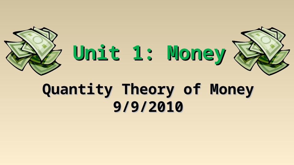
Learning MethodsLearning MethodsThree economic languagesThree economic languages• verbal (words)• algebraic (math)• graphical (diagrams)
Equation of ExchangeEquation of ExchangeThe equation of exchange is the fundamental
mathematical idea of monetary theory.
MSV = Py
DefinitionsDefinitionspurchasing power of money (PPM) purchasing power of money (PPM) –
the basket of goods and services that asingle dollar can buy (“price” of money)
price level (P) price level (P) –weighted average of prices in the economy
PPM ≡ 1/PPP
DefinitionsDefinitionsPrice level is stated in terms of price indexes.
Price indexes are inherently imprecise because you have to pick goods to include in the index and weight them.
There is no price index that includes everything.
Government price indexesGovernment price indexes• consumer price index (CPI)• producer price index (PPI)• GDP deflator
DefinitionsDefinitionsinflation inflation –
a rise in the price level (fall in PPM)
deflation deflation –a fall in the price level (rise in PPM)
DefinitionsDefinitions
relative prices relative prices –implicit barter ratios between goods
Price levels move independently of relative prices.
If the relative price of one thing goes up, logically the relative price of another thing must go down.
DefinitionsDefinitionsreal variables real variables – “constant” dollars
nominal variables nominal variables – “current” dollars
Capital letter variables are nominal. Lowercase letter variables are real.
nominal/P = real
Y/P = y
DefinitionsDefinitionsaggregate output aggregate output –
total production of finalgoods and services in the economy
aggregrate income aggregrate income –Total income of factors of production(land, labor, capital) in the economy
For our purposes:Y ≡ aggregate output = aggregate income
YY
DefinitionsDefinitionsY ≡ nominal output
y ≡ real output
Y/P = yPy = Y
In the equation of exchange,we use a lowercase y (real output)
rather than capital Y (nominal output).This is more precise than Mishkin’s notation.
yy
DefinitionsDefinitionsMS ≡ money supply
The money supply can bein terms of any of themonetary aggregates:
M1, M2, M3, MB, MZM.
Again, we will use more precise notation than Mishkin, which just
uses M instead of MS.
MS
DefinitionsDefinitionsMS/P ≡ real money stock
real money balance real money balance –quantity of money in real terms
Real money balance is an important concept in the
Keynesian money demand theory and in later studies of seigniorage.
MS/P
DefinitionsDefinitionsvelocity of money (V) –
average number of times a unit of money turns over in a given period
Velocity is defined as total spending divided by the quantity of money:
V ≡ Py/MS
So the equation of exchange is an identity: MSV = Py
V
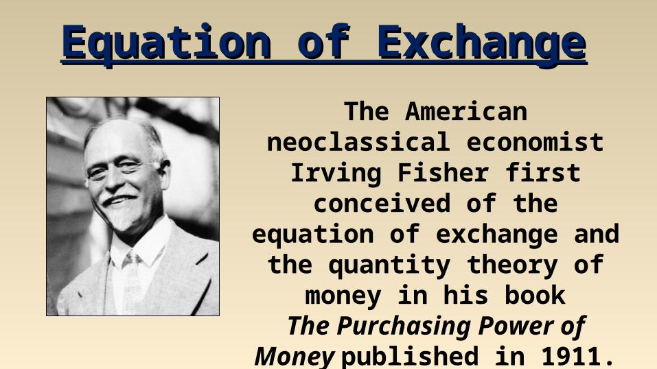
Equation of ExchangeEquation of ExchangeThe American neoclassical
economist Irving Fisher first conceived of the equation of
exchange and the quantity theory of money in his book
The Purchasing Power of Money published in 1911.
Equation of ExchangeEquation of ExchangeFisher originally conceived the equation
of exchange with all transactions instead of all final transactions.
Fisher versionMSVT = Pt
Modern version:MSV = Py
Equation of ExchangeEquation of Exchange
MSV = PyImportant notesImportant notes• an identity, not a theory (V ≡ Py/MS)• right side is nominal output (Y = Py)• MS can be any monetary aggregate (changing the aggregate changes V)
Quantity Theory of MoneyQuantity Theory of MoneyThe quantity theory of money conceived by Irving
Fisher makes two important assumptions.
AssumptionsAssumptions1. velocity is constant2. wages and prices are completely flexible
V
Quantity Theory of MoneyQuantity Theory of MoneyIf velocity is constantV then ΔMS → ΔPy
(doubling MS will double Py).VMS = Py
If P is completely flexible and y is sticky,assumey: ΔMS → ΔP
(doubling MS will double P).VMS = yP
Quantity Theory of MoneyQuantity Theory of MoneyApplying the quantity theory of money,
the equation of exchange can bereformulated into the Cambridge equation
to make the intuition clearer.
k ≡ 1/V (a constant)MSV = Py
MS = (1/V)Py
MS = kPy
k
Graphical VersionGraphical VersionWe write MS instead of the M Mishkin uses.
MSV = PyThis is to save us a step.
We should use money demand not money supply:MDV = Py
But we equilibrate demand with supply:MS = MD
Therefore:MSV = Py
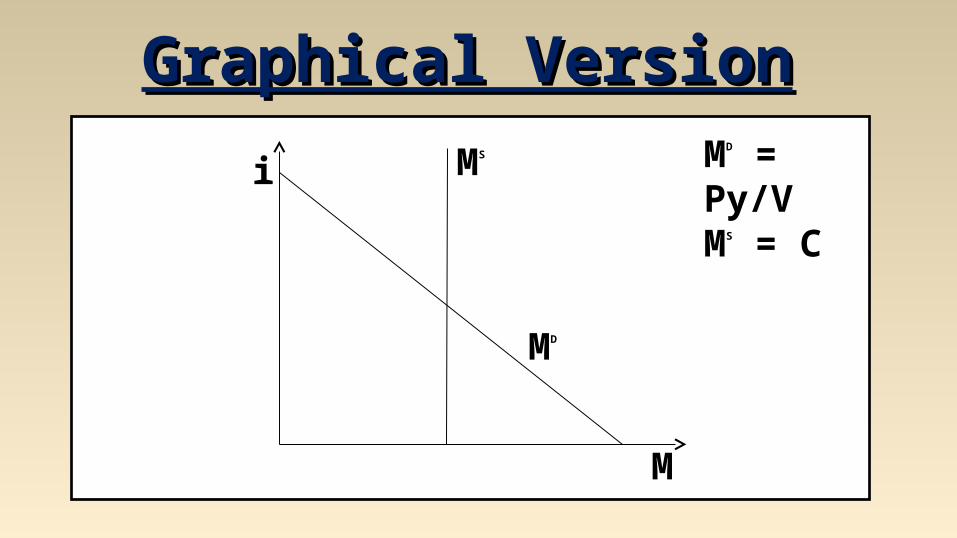
Graphical VersionGraphical VersionThe graphical version uses the money demand equation
and the money supply equation to find equilibrium.
Money demand:MD = Py/V
Money supply:MS = C
(C is a constant)
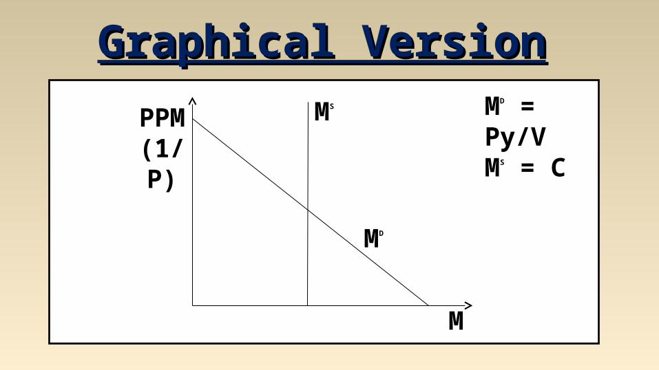
Graphical VersionGraphical VersionMD = Py/VMS = C
MD
MS
PPM(1/P)
M
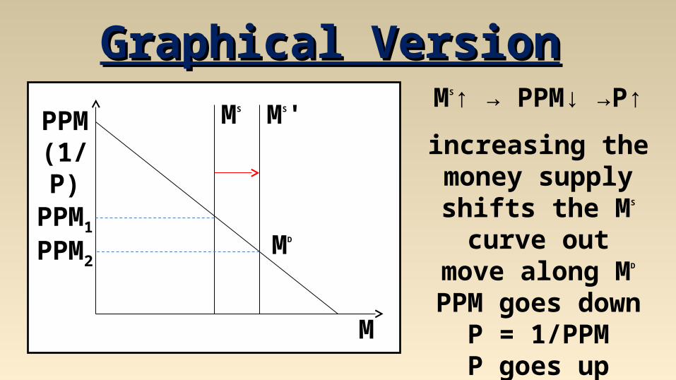
Graphical VersionGraphical VersionMS↑ → PPM↓ →P↑
increasing themoney supply
shifts the MS curve outmove along MD
PPM goes downP = 1/PPMP goes up
MD
MS
PPM(1/P)
M
MS'
PPM1
PPM2
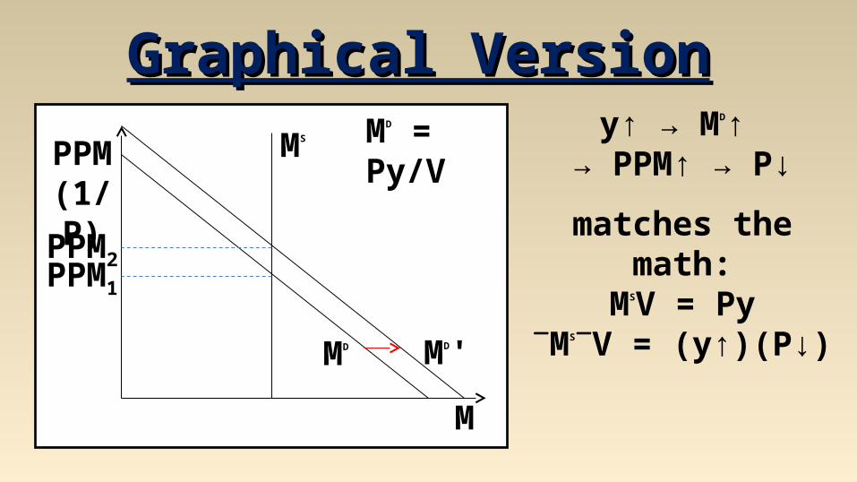
Graphical VersionGraphical Version
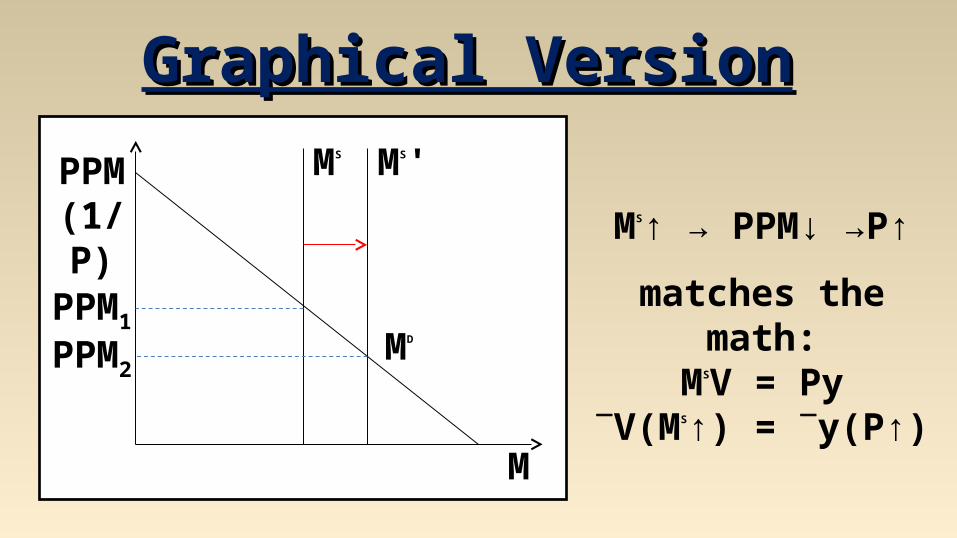
MS↑ → PPM↓ →P↑
matches the math:MSV = Py
V(MS↑) = y(P↑)MD
MS
PPM(1/P)
M
MS'
PPM1
PPM2
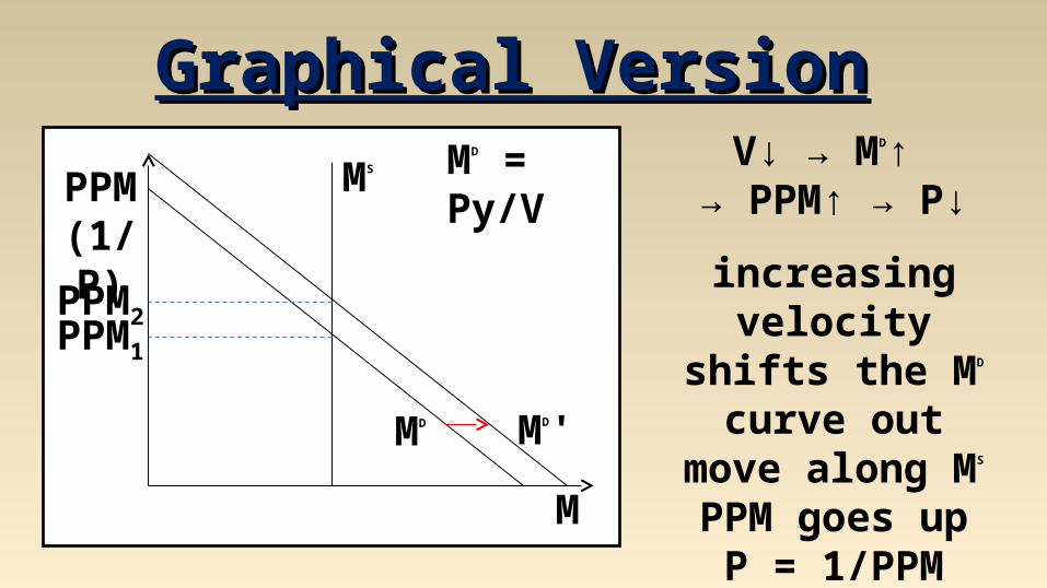
Graphical VersionGraphical VersionV↓ → MD↑
→ PPM↑ → P↓
increasing velocityshifts the MD curve out
move along MS
PPM goes upP = 1/PPM
P goes down
PPM(1/P)
PPM1
PPM2
MD'
MS
M
MD
MD = Py/V

Graphical VersionGraphical VersionV↓ → MD↑
→ PPM↑ → P↓
matches the math:MSV = Py
MS(V↓) =y(P↓)
PPM(1/P)
PPM1
PPM2
MD'
MS
M
MD
MD = Py/V
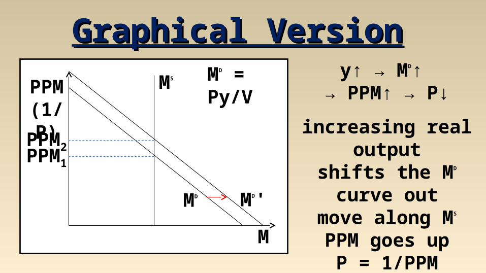
Graphical VersionGraphical Versiony↑ → MD↑
→ PPM↑ → P↓
increasing real outputshifts the MD curve out
move along MS
PPM goes upP = 1/PPM
P goes down
PPM(1/P)
PPM1
PPM2
MD'
MS
M
MD
MD = Py/V
Graphical VersionGraphical Versiony↑ → MD↑
→ PPM↑ → P↓
matches the math:MSV = Py
MSV = (y↑)(P↓)
PPM(1/P)
PPM1
PPM2
MD'
MS
M
MD
MD = Py/V
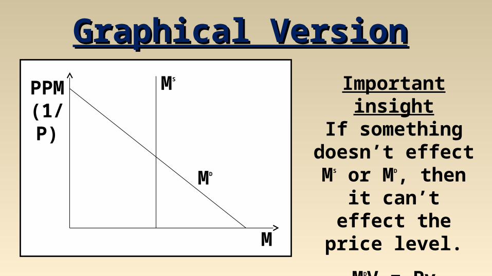
Graphical VersionGraphical VersionImportant insight
If something doesn’t effect MS or MD, then
it can’t effect the price level.
MDV = PyMS = C
MD
MS
PPM(1/P)
M
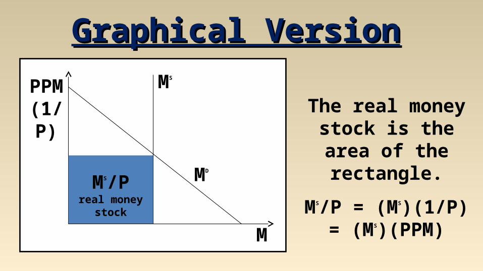
Graphical VersionGraphical Version
The real money stock is the area of the
rectangle.
MS/P = (MS)(1/P)= (MS)(PPM)
MD
MS
PPM(1/P)
M
MS/Preal money stock
But empirical evidence shows that velocity is not a constant.
Velocity declines during severe economy contractions.
Even in the short run velocity fluctuates too much to be viewed as constant.
This paved the way for a new theory.
VLiquidity Preference TheoryLiquidity Preference Theory
John Maynard Keynes,the father of macroeconomics, wrote The General Theory of Employment,
Interest, and Money in 1936.His theory of demand for money,
which he called the liquidity preference theory, explored the question “Why do
individuals hold money?
Liquidity Preference TheoryLiquidity Preference Theory
Liquidity Preference TheoryLiquidity Preference TheoryKeynes’ reasons individuals hold moneyKeynes’ reasons individuals hold money• transactions motive• precautionary motive• speculative motive
Liquidity Preference TheoryLiquidity Preference Theorytransactions motive transactions motive –
money is a medium of exchangethat can be used to carry out
everyday transactions
Keynes believed transactionswere proportional to income.
Thus the transactions componentof MD depends entirely on y.
Liquidity Preference TheoryLiquidity Preference Theoryprecautionary motive precautionary motive –
people hold money as a cushion against an unexpected purchase need
Keynes thought precautionary balances were based on future transactions, and
thus were proportional to income.Thus the precautionary component
of MD depends entirely on y.
Liquidity Preference TheoryLiquidity Preference Theoryspeculative motive speculative motive –
people hold money as analternative store of wealth to bonds
Keynes thought people would switch from bonds to money when they believed bond values would fall.
Thus the precautionary componentof MD depends on the interest rate.
Liquidity Preference TheoryLiquidity Preference TheoryKeynes thought interest rates should be in a narrow band. When interest
rates are higher than the band, people expect them to fall. When lower than the band, people expect them to rise.
If interest rates rise, then the price of a bond falls. So if you expect interest
rates to rise, you expect a capital loss from holding bonds.
Liquidity Preference TheoryLiquidity Preference TheoryKeynes’ reasons individuals hold moneyKeynes’ reasons individuals hold money• transactions motive (positively related to y)• precautionary motive (positively related to y)• speculative motive (negatively related to i)
MD/P = f(i,y)fi = –fy = +
P/MD = 1/f(i,y)Py/MD = y/f(i,y)V = y/f(i,y)
Liquidity Preference TheoryLiquidity Preference Theory
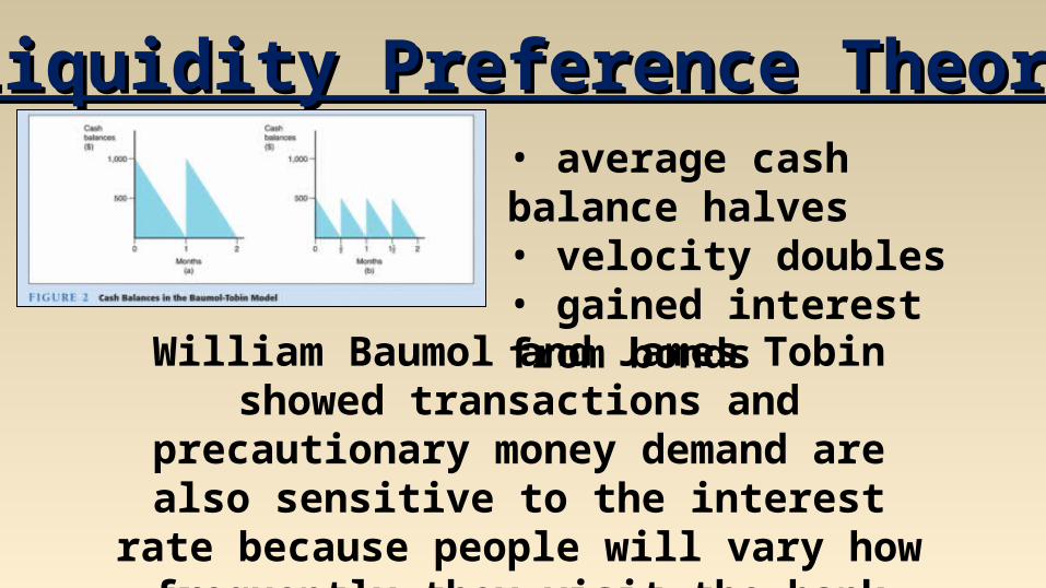
William Baumol and James Tobin showed transactions and precautionary money demand are also sensitive to the interest rate because people will vary how frequently they visit the
bank based on interest rates.
• average cash balance halves• velocity doubles• gained interest from bonds
Liquidity Preference TheoryLiquidity Preference Theorytransactions demand transactions demand –
money demand for transactions
VectorsVectors• population: N↑ → y↑ → MD↑ → P↓• output/person: y/N↑ → y↑ → MD↑ → P↓• vertical integration: merge↑ → MD↓ → P↑• clearing system efficiency: eff.↑ → MD↓ → P↑
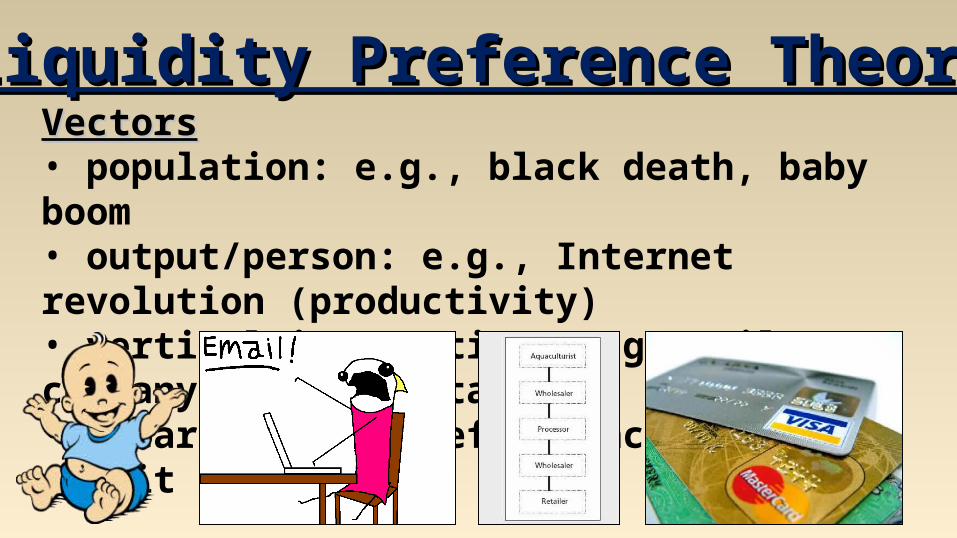
Liquidity Preference TheoryLiquidity Preference TheoryVectorsVectors• population: e.g., black death, baby boom• output/person: e.g., Internet revolution (productivity)• vertical integration: e.g., oil company buys gas stations• clearing system efficiency: e.g., credit card use
Liquidity Preference TheoryLiquidity Preference Theoryportfolio demand portfolio demand –
money demand as a store of value(captures precautionary and speculative)
VectorsVectors• wealth: W↑ → MD↑ → P↓• uncertainty: uncertainty↑ → MD↑ → P↓• interest differential: i↑ → MD↓ → P↑• anticipations about inflation: πe↓ → MD↑ → P↓
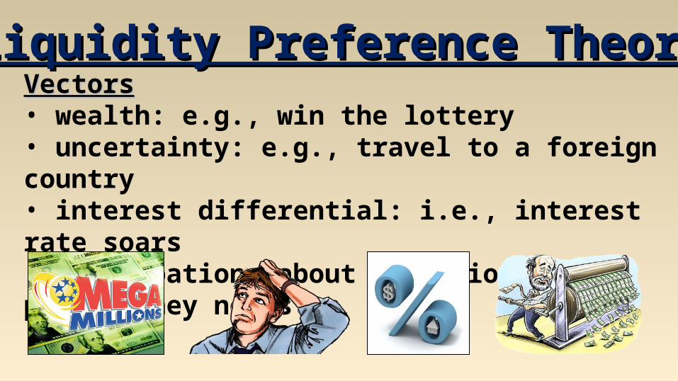
Liquidity Preference TheoryLiquidity Preference TheoryVectorsVectors• wealth: e.g., win the lottery• uncertainty: e.g., travel to a foreign country• interest differential: i.e., interest rate soars• anticipations about inflation: e.g., print money non-stop
Graphical VersionGraphical VersionMD = Py/VMS = C
MD
MS
i
M
Graphical VersionGraphical Version
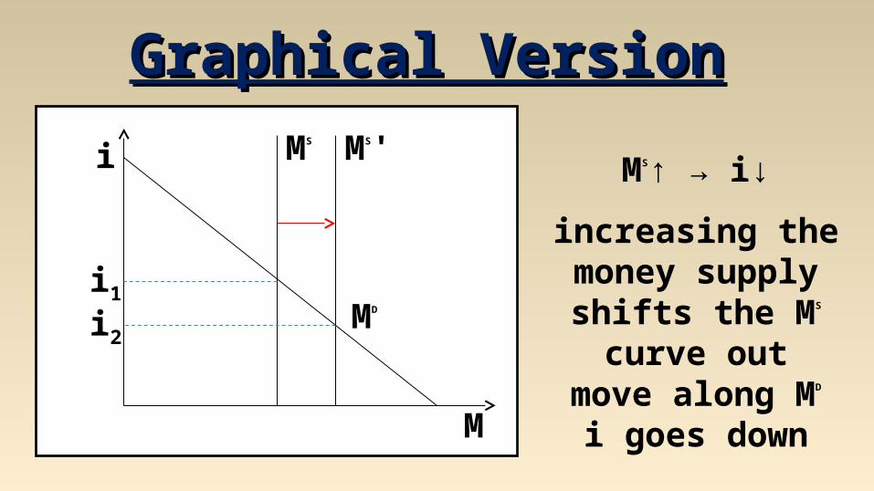
MS↑ → i↓
increasing themoney supply
shifts the MS curve outmove along MD
i goes down
MD
MS
i
M
MS'
i1
i2
Graphical VersionGraphical Version
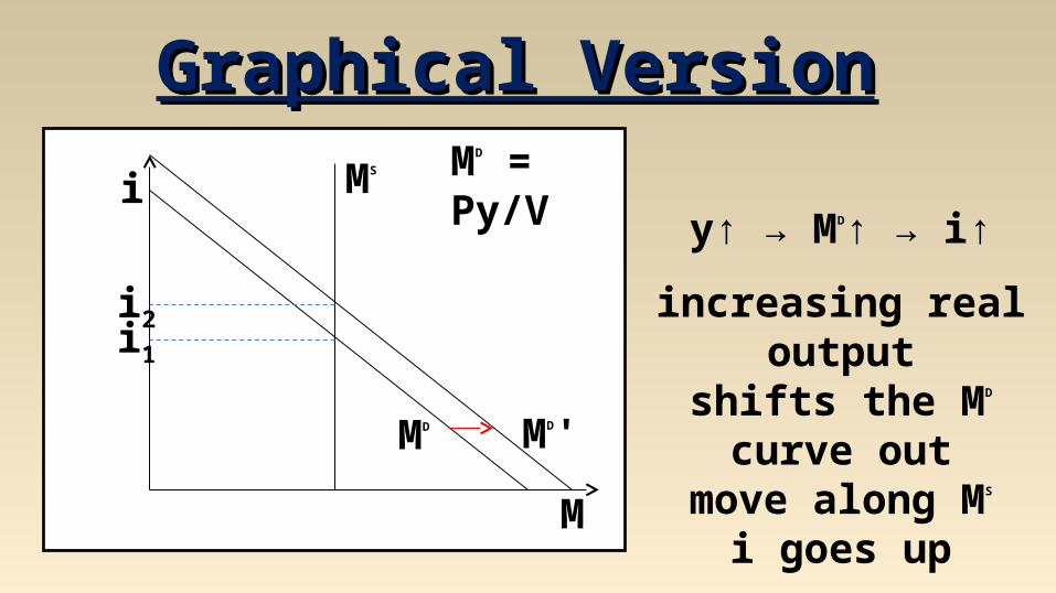
y↑ → MD↑ → i↑
increasing real outputshifts the MD curve out
move along MS
i goes up
i
i1
i2
MD'
MS
M
MD
MD = Py/V
Graphical VersionGraphical Version
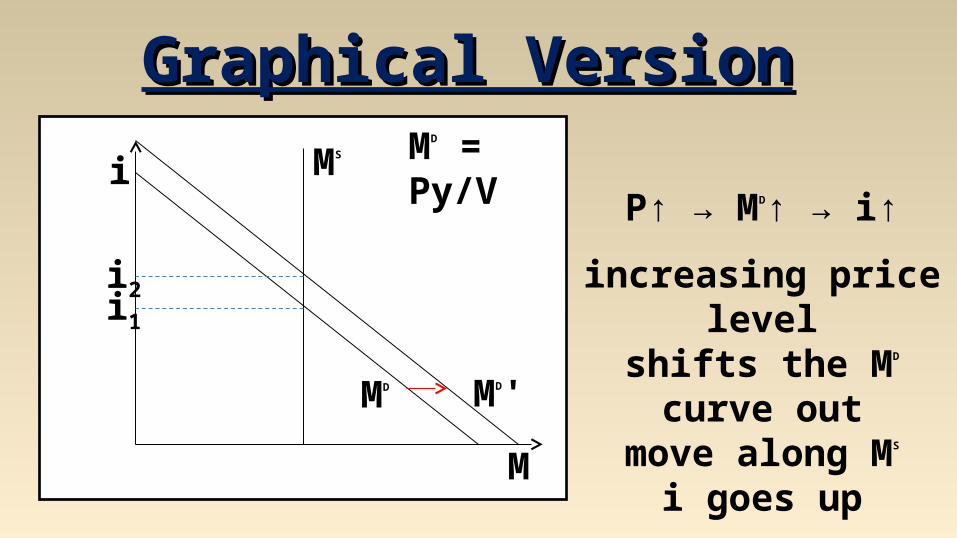
P↑ → MD↑ → i↑
increasing price levelshifts the MD curve out
move along MS
i goes up
i
i1
i2
MD'
MS
M
MD
MD = Py/V
Modern Quantity TheoryModern Quantity TheoryMilton Friedman is a Nobel prize
winning economist from the Chicago school who led the free market fight
against Keynesianism in the 60’s, 70’s, and 80’s. He developed a modern
quantity theory of money based on his permanent income hypothesis and an
expanded asset demand theory.
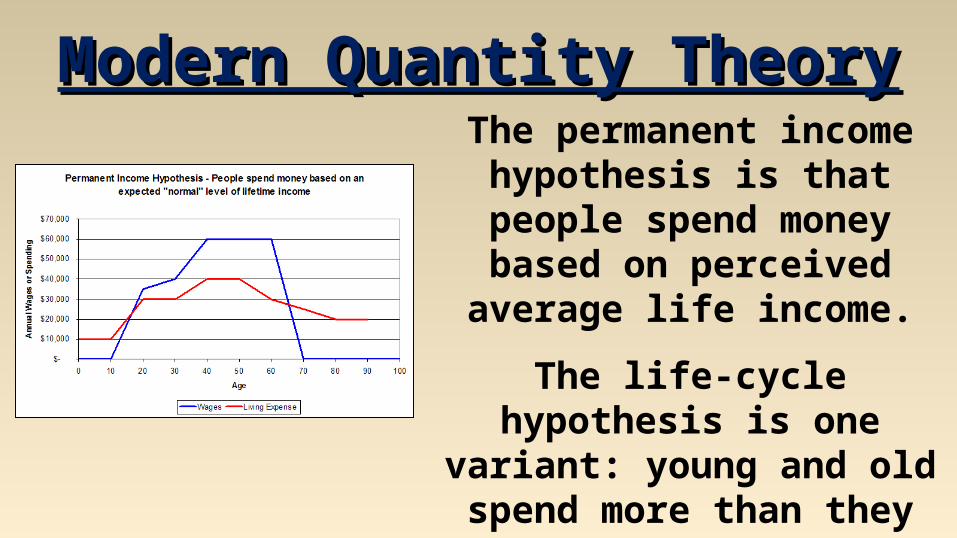
Modern Quantity TheoryModern Quantity TheoryThe permanent income
hypothesis is that people spend money based on perceived
average life income.
The life-cycle hypothesis is one variant: young and old spend more than they earn, middle
age earn more than they spend.
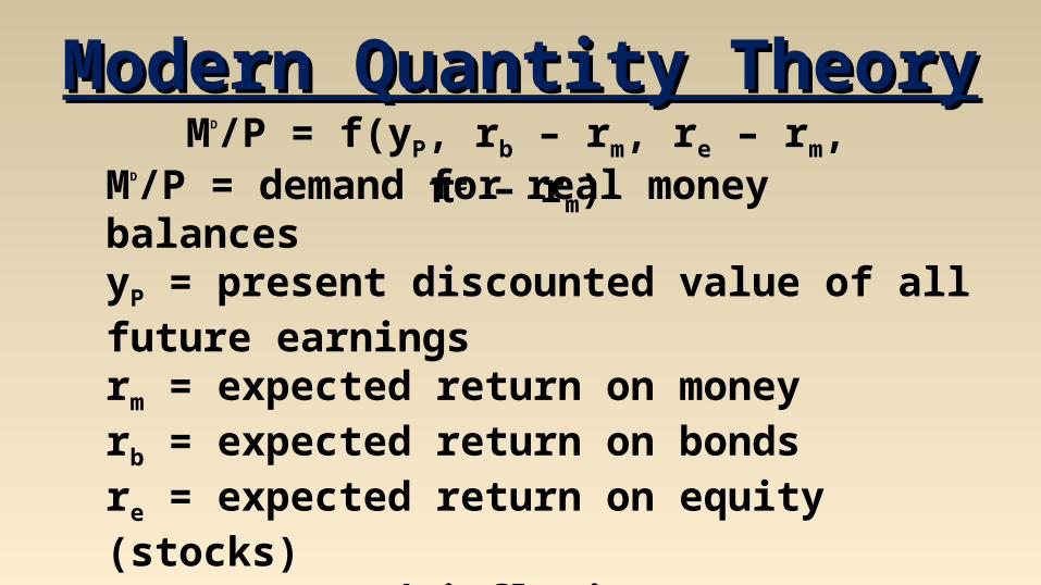
Modern Quantity TheoryModern Quantity TheoryMD/P = f(yP, rb – rm, re – rm, πe – rm)
MD/P = demand for real money balancesyP = present discounted value of all future earningsrm = expected return on moneyrb = expected return on bondsre = expected return on equity (stocks)πe = expected inflation rate
MD positively correlated to yP
MD negatively correlated to other terms
Modern Quantity TheoryModern Quantity Theory
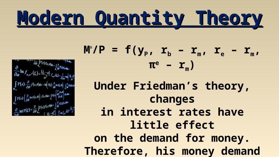
MD/P = f(yP, rb – rm, re – rm, πe – rm)
Under Friedman’s theory, changesin interest rates have little effect
on the demand for money.Therefore, his money demand
equation can be approximated by:
MD/P = f(yP)
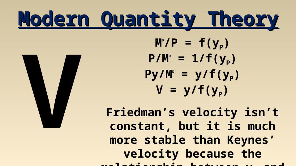
MD/P = f(yP)P/MD = 1/f(yP)Py/MD = y/f(yP)
V = y/f(yP)
Friedman’s velocity isn’t constant, but it is much more stable than Keynes’ velocity because the relationship
between yP and y is very predictable.
VModern Quantity TheoryModern Quantity Theory
Empirical EvidenceEmpirical Evidence
Empirical evidence shows thatvelocity is not constant.
Velocity is sensitive to interest rates,but is not ultra-sensitive to interest rates
when interest rates are non-zero(i.e., there is no liquidity trap).
V