Unit 1: Money Bonds & Stock Market 9/21/2010. Definitions risk structure of interest rates risk...

Unit 1: MoneyUnit 1: Money

Bonds & Stock MarketBonds & Stock Market9/21/20109/21/2010

DefinitionsDefinitionsrisk structure of interest rates risk structure of interest rates –

the relationship among the interest rates on various bonds with the same term to maturity

term structure of interest rates term structure of interest rates –the relationship among the interest rates on

various bonds with different terms to maturity

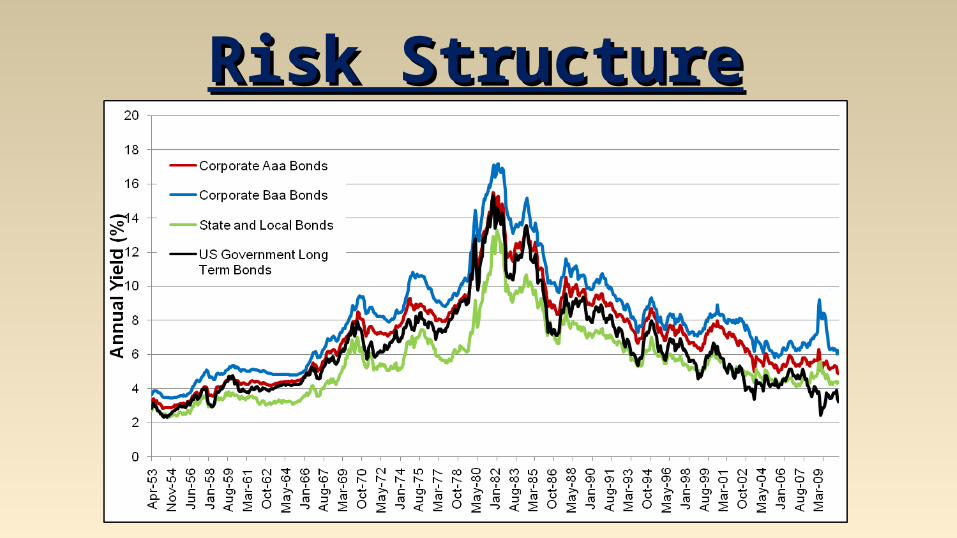
Risk StructureRisk Structure

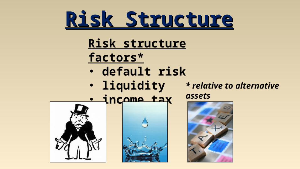
Risk structure factors*• default risk• liquidity• income tax


* relative to alternative assets

default default –party issuing debt instrument is

unable to make interest payments orpay off the amount owed at maturity

default-free bonds default-free bonds –bonds with no default risk

risk premium risk premium –interest rate spread between bonds with

default risk and default-free bonds


Mishkin claims that federal government bonds are default-free.

But just because a government can theoretically pay off a bond doesn’t

mean it can credibly commit to do so or will follow through in practice.

Many governments have defaulted.


Corporate bondsriskc↑ → BD

c↓ → PBc↓ → iBc↑(Re

c ↓ → BD

c↓ → PBc↓ → iBc↑)

Treasury bondsriskT↓ → BD

T↑ → PBT↑ → iBT↓(Re

T↑ → BD

T↑ → PBT↑ → iBT↓)

risk premium (iBc – iBT)↑

Risk is relative to alternative assets.


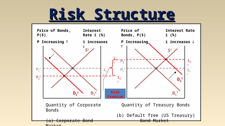
Risk StructureRisk StructurePrice of Bonds, P($)

P Increasing

Interest Rate i (%)

i increases

Quantity of Corporate Bonds

(a) Corporate Bond Market

Price of Bonds, P($)

P Increasing

Interest Rate i (%)

i increases

Quantity of Treasury Bonds

(b) Default free (US Treasury) Bond Market

D1c

Sc

D1T

ST

P1C i1

C P1T i1

T

D2c

D2T

P2T i2

T

Risk Premium

i2T

P2C i2

C

Risk StructureRisk StructureA bond with a default risk will

always have a positive risk premium, and an increase in default

risk will raise the risk premium.

Credit rating agencies rate the quality of bonds in terms of

probability of default.AAA less likely to default than CCC.

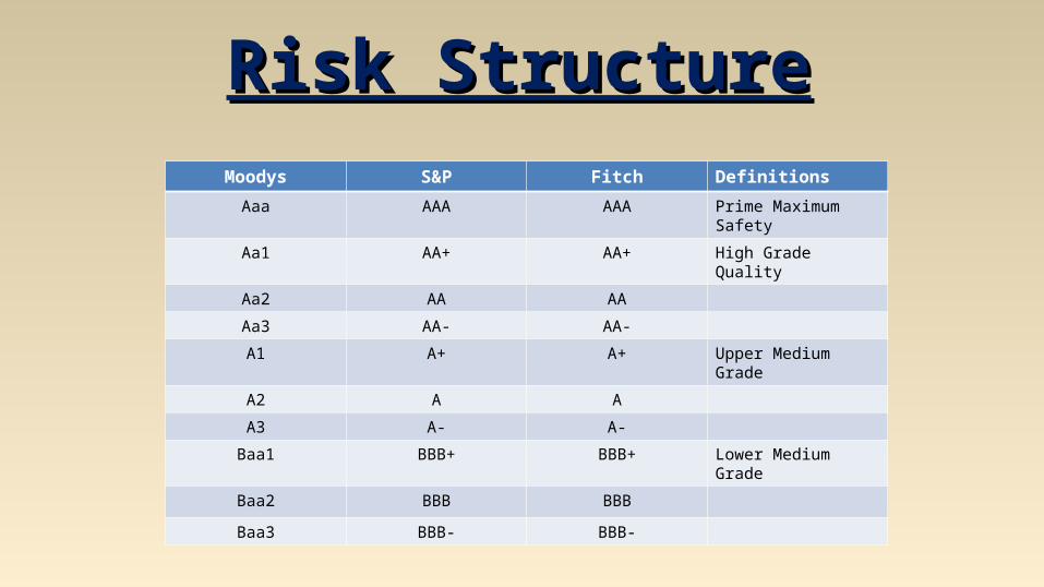
Risk StructureRisk StructureMoodys S&P Fitch Definitions

Aaa AAA AAA Prime Maximum Safety

Aa1 AA+ AA+ High Grade Quality

Aa2 AA AA

Aa3 AA- AA-

A1 A+ A+ Upper Medium Grade

A2 A A

A3 A- A-

Baa1 BBB+ BBB+ Lower Medium Grade

Baa2 BBB BBB

Baa3 BBB- BBB-

Risk StructureRisk StructureMoodys S&P Fitch Definitions

Ba1 BB+ BB+ Non Investment Grade

Ba2 BB BB Speculative

Ba3 BB- BB-

B1 B+ B+ Highly Speculative

B2 B B

B3 B- B-

Caa1 CCC+ CCC Substantial Risk

Caa2 CCC - In poor standing

Caa3 CCC- -

Ca - - Extremely speculative

C - - May be in default

- - DDD Default

- - DD -

- D D


As we’ll see later when we discuss the sub-prime crisis, rating

agencies are very unreliable.

Risk StructureRisk StructureMishkin speaks derisively of “junk

bonds”. In reality so-called junk bonds were high yield corporate bonds that

funneled money to productive companies. They short-circuited venture capital / private equity /

investment banks / hedge funds, going directly to individual investors instead.

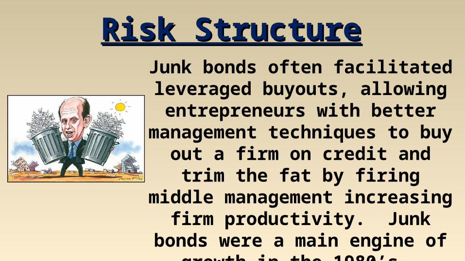
Risk StructureRisk StructureJunk bonds often facilitated leveraged buyouts, allowing entrepreneurs with better management techniques to buy out a firm on credit and trim the fat by firing middle management increasing firm productivity. Junk bonds were a main engine of growth in the 1980’s. Michael Milken, the “junk bond king,”

was a hero, not a villain.

Higher liquidity relative to alternative assets increases the demand for bonds.

Liquidity is lumped into the risk structure of interest rates even though the classification is a bit of a misnomer.


Risk StructureRisk StructureCorporate bondsliquidityc↓ → BD

c↓ → PBc↓ → iBc↑

Treasury bondsliquidityT↑ → BD

T↑ → PBT↑ → iBT↓

risk premium (iBc – iBT)↑

Liquidity is relative to alternative assets.


P Increasing

Interest Rate i (%)

i increases

Quantity of Corporate Bonds

(a) Corporate Bond Market


P Increasing

Interest Rate i (%)

i increases

Quantity of Treasury Bonds

(b) Default free (US Treasury) Bond Market

D1c

Sc

D1T

ST

P1C i1

C P1T i1

T

D2c

D2T

P2T i2

T

Risk Premium

i2T

P2C i2

C


Risk StructureRisk StructureMunicipal bonds have a lower yield than federal bonds even though they have a

higher default risk. Why?

Income from municipal bonds isnot taxed by the federal government

due to state sovereignty reasons(11th amendment).


Just as lowering risk raises expected return, making bond income tax-free

similarly raises expected return.

Municipal bondstaxesM↓ → BD

M↑ → PBM↑ → iBM↓(Re

M↑ → BD

M↑ → PBM↑ → iBM↓)

Treasury bondstaxesT↑ → BD

T↓ → PBT↓ → iBT↑(Re

T↓ → BD

T↓ → PBT↓ → iBT↑)

Taxes are relative to alternative assets.


Risk structure factors• default risk: riskB↑ → BD↓ → PB↓• liquidity: liquidityB↓ → BD↓ → PB↓• income tax: taxB↓ → BD↑ → PB↑


Term StructureTerm Structureyield curve yield curve –

plot of the yields of bonds with differingterms to maturity but the same risk structure

(risk, liquidity, and tax considerations)

inverted yield curve inverted yield curve –downward sloping yield curve

Term StructureTerm Structure

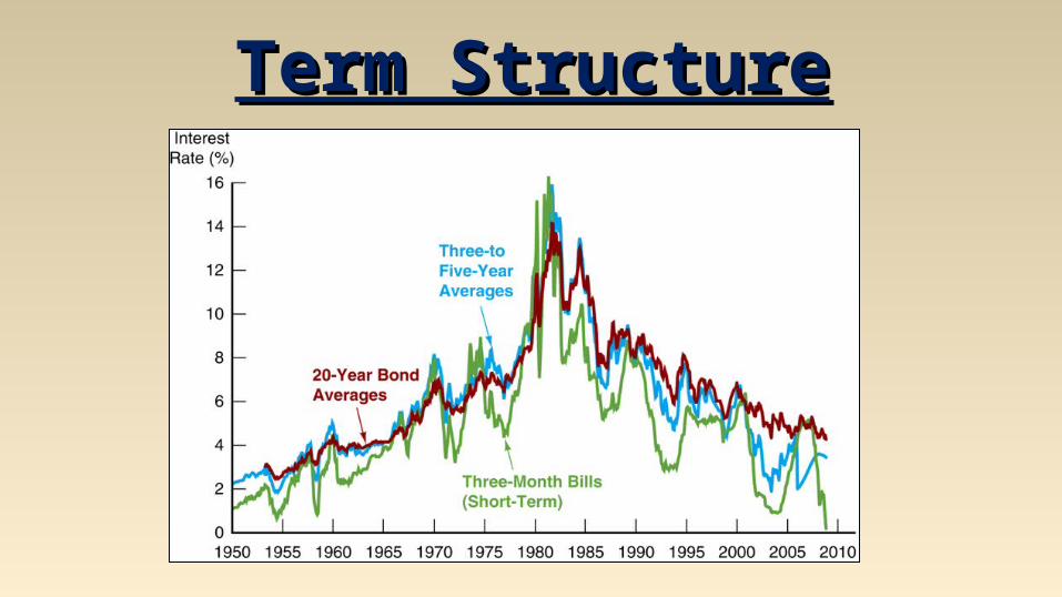
Term structure empirical facts1.interest rates on bonds of different maturities move together over time2.low short-term interest rates usually mean upward sloping yield curves; high short-term interest rates usually mean downward sloping yield curves3.yield curves almost always slope upward


Term structure theories• expectations theory• segmented markets theory• liquidity premium theory / preferred habitat theory


Term StructureTerm Structureexpectations theory expectations theory –

the interest rate of a long-term bond will equal the average of short-term interest rates people expect over the

life of the long-term bond

• Assumption: Bonds of different maturities are perfect substitutes.• Implication: Re on bonds of different maturities are equal.


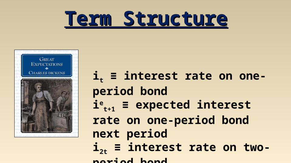
it ≡ interest rate on one-period bondie

t+1 ≡ expected interest rate on one-period bond next periodi2t ≡ interest rate on two-period bond

Term StructureTerm StructureExpected return from two-period bond(1 + i2t)(1 + i2t) – 1 = 1 + 2i2t + (i2t)2 – 1= 2i2t + (i2t)2 ≈ 2i2t

Expected return from one-period bond(1 + it)(1 + ie

t+1) – 1 = 1 + it + iet+1 + it(ie

t+1) – 1 = it + ie

t+1 + it(iet+1) ≈ it + ie

t+1

Re equal2i2t = it + ie

t+1


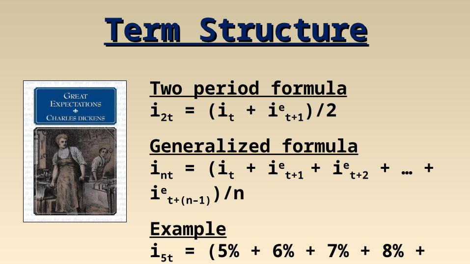
Two period formulai2t = (it + ie

t+1)/2

Generalized formulaint = (it + ie

t+1 + iet+2 + … + ie

t+(n–1))/n

Examplei5t = (5% + 6% + 7% + 8% + 9%)/5 = 7%

Term StructureTerm StructureExplains Fact 1 that short and long rates move together:

• Short rate rises are persistent• it↑ → it+1↑, it+2↑, etc. → average of future rates int↑• Therefore: it↑ → int↑, i.e., short and long rates move together


Explains Fact 2 that yield curves tend to have steep slope when short rates are low and downward slope when short rates are high:


When short rates are low, they are expected to rise to normal level, and long rate = average of future short rates will be well above today’s short rate: yield curve will have steep upward slope


When short rates are high, they will be expected to fall in future, and long rate will be below current short rate: yield curve will have downward slope

Term StructureTerm StructureDoesn’t explain Fact 3 that yield curve usually has upward slope:

Short rates as likely to fall in future as rise, so average of future short rates will not usually be higher than current short rate: therefore, yield curve will not usually slope upward

Term StructureTerm Structuresegmented markets theory segmented markets theory –

markets for different maturity bonds are completely separate;

interest rates are determined by supply and demand for that bond only

• Assumption: Bonds of different maturities are not substitutes.• Implication: Interest rate at each maturity determined seperately.

Term StructureTerm StructureExplains Fact 3 that yield curve is usually upward sloping:

People typically prefer short holding periods and thus have higher demand for short-term bonds, which have higher price and lower interest rates than long bonds.


Does not explain Fact 1 or Fact 2 because assumes long and short rates

determined independently.


liquidity premium theory liquidity premium theory –the interest rate of a long-term bond will equal the average of short-term interest rates people expect over the

life of the long-term bondplus a liquidity premium


• Assumption: Bonds of different maturities are substitutes, but not perfect substitutes.• Implication: Modifies expectations theory with features of segmented markets theory.

Term StructureTerm StructureInvestors prefer short rather than long bonds, so they must be paid positive liquidity (term) premium, lnt, to hold

long-term bonds.

lnt ≡ liquidity premium forn-period bond at time t

lnt always positive, rises with maturity.


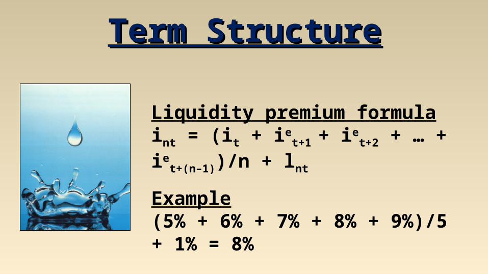
Liquidity premium formulaint = (it + ie

t+1 + iet+2 + … + ie

t+(n–1))/n + lnt

Example(5% + 6% + 7% + 8% + 9%)/5 + 1% = 8%


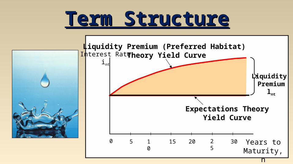
Interest Rateint

Years to Maturity, n

0 5 10 15 20 25 30

Expectations TheoryYield Curve

Liquidity Premium

lnt

Liquidity Premium (Preferred Habitat) Theory Yield Curve


Explains Fact 1 that short and long rates move together:

Interest rates on different maturity bonds move together over time; explained by the first term in the equation.

Term StructureTerm StructureExplains Fact 2 that yield curves tend to slope up when short rates are low and slope down when short rates are high:

Yield curves tend to slope upward when short-term rates are low and to be inverted when short-term rates are high; explained by the liquidity premium term in the first case and by a low expected average in the second case.


Explains Fact 3 that yield curve is usually upward sloping:

Yield curves typically slope upward; explained by a larger liquidity premium as the term to maturity lengthens

Term structure theories• expectations theory: explains 1 & 2, not 3• segmented markets theory: explains 3, not 1 & 2• liquidity premium theory: explains 1, 2, & 3


Interpreting yield curvesInterpreting yield curves

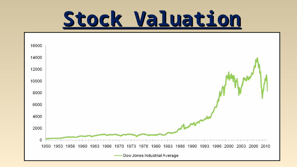
Stock ValuationStock Valuation

Current stock values are the present discounted value of

future dividends.


One-Period Stock Valuation Modelp0 ≡ current price of stockD1 ≡ dividend paid for year 1ke ≡ required return in equityp1 ≡ stock price at the end of year 1

p0 = D1/(1 + ke) + p1/(1 + ke)


Generalized Stock Valuation Model

with final sale:p0 = D1/(1 + ke)1 + D2/(1 + ke)2 +

… + Dn/(1 + ke)n + pne/(1 + ke)n

without final sale:p0 = ∑Dt/(1 + ke)t

Stock ValuationStock ValuationGeneralized Stock Valuation Model

model:p0 = D1/(1 + ke)1 + D2/(1 + ke)2 +

… + Dn/(1 + ke)n + pne/(1 + ke)n

fundamentals:D1/(1 + ke)1 + … + Dn/(1 + ke)n

bubble:pn

e/(1 + ke)n

Stock ValuationStock ValuationGordon Growth ModelD0 ≡ most recent dividend paidg ≡ expected constant growth rate

p0 = D0(1 + g)1/(1 + ke)1 +D0(1 + g)2/(1 + ke)2 + … +D0(1 + g)∞/(1 + ke)∞

simplified:p0 = D0(1 + g)/(ke – g) = D1/(ke – g)

Setting PricesSetting Prices

• uncertainty↑ → ke↑ → p0↓• economy growth↑ → g↑ → p0↑• dividends↑ → D0↑ → p0↑

Setting PricesSetting Prices• The price is set by the buyer willing to pay the highest price.• The market price will be set by the buyer who can take best advantage of the asset.• Superior information about an asset can increase its value by reducing its perceived risk.

Setting PricesSetting Prices• Information is important for individuals to value each asset.• When new information is released about a firm, expectations and prices change.• Market participants constantly receive information and revise their expectations, so stock prices change frequently.

ExpectationsExpectationsadaptive expectations adaptive expectations –

expectations are formed from past experience only

rational expectations rational expectations –expectations will be identical

to optimal forecasts(the best guess of the future)

using all available information

ExpectationsExpectations

Adaptive expectations• Expectations are formed from past experience only.• Changes in expectations will occur slowly over time as data changes.

ExpectationsExpectationsRational expectations• Boils down to assuming agents use the same model of the economy as the researcher (“model-consistent”).• People can make mistakes, but they do not make systematic forecasting errors.• Optimal prediction, may not be accurate.• It is costly not to have optimal forecast.• Xe = Xof = Et [ X | Ωt ]

Efficient Market HypothesisEfficient Market Hypothesis

efficient market hypothesis efficient market hypothesis –applies rational expectations

to financial markets;stock prices reflect

all available information

Efficient Market HypothesisEfficient Market HypothesisEfficient market hypothesis• weak form – stock prices reflect past stock price history• semi-strong form – stock prices reflect all publicly available information• strong form – stock prices reflect all information (public and insider)

Efficient Market HypothesisEfficient Market Hypothesisarbitrage arbitrage –

market participants eliminate unexploited profit opportunities

Arbitrage is the mechanism tending toward the efficient market hypothesis.

Rof > R* → pt↑ → Rof↓Rof < R* → pt↓ → Rof↑

until… Rof = R*

Efficient Market HypothesisEfficient Market Hypothesis• The optimal forecast of a security’s return using all available information equals the security’s equilibrium return.• In an efficient market, a security’s price fully reflects all available information.• All unexploited profit opportunities will be eliminated.• Efficient market holds even if there are some uninformed, irrational participants.

Efficient Market HypothesisEfficient Market HypothesisFavorable evidence• Investment analysts and mutual funds don’t beat the market• Stock prices reflect publicly available information: anticipated announcements don’t affect stock price• Stock prices close to random walk• Technical analysis doesn’t outperform market

Efficient Market HypothesisEfficient Market HypothesisUnfavorable evidence• Small-firm effect: small firms have abnormally high returns• January effect: high returns in January• Market overreaction• Excessive volatility• Mean reversion• New information is not always immediately incorporated into prices

Efficient Market HypothesisEfficient Market HypothesisImplications• Published reports of financial analysts not very valuable• Should be skeptical of hot tips• Stock prices may fall on good news• Prescription for investor

o Shouldn’t try to outguess marketo Buy and holdo Diversify with no-load mutual fund

Unit 1: Money Bonds & Stock Market 9/21/2010. Definitions risk structure of interest rates risk...

Documents

Transcript of Unit 1: Money Bonds & Stock Market 9/21/2010. Definitions risk structure of interest rates risk...