
Unit 1: 12 hrs. · · 2018-01-17Distributed vs Centralized Database System; advantages and ......
113
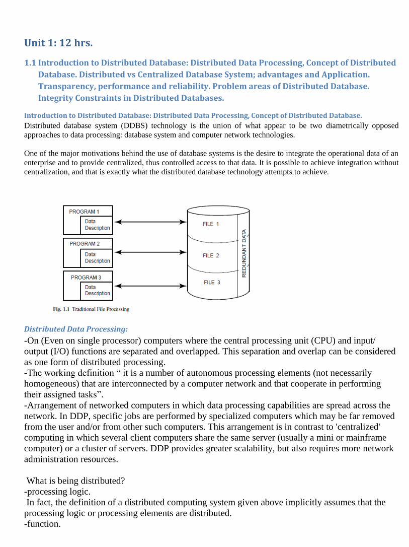
Unit 1: 12 hrs. 1.1 Introduction to Distributed Database: Distributed Data Processing, Concept of Distributed Database. Distributed vs Centralized Database System; advantages and Application. Transparency, performance and reliability. Problem areas of Distributed Database. Integrity Constraints in Distributed Databases. Introduction to Distributed Database: Distributed Data Processing, Concept of Distributed Database. Distributed database system (DDBS) technology is the union of what appear to be two diametrically opposed approaches to data processing: database system and computer network technologies. One of the major motivations behind the use of database systems is the desire to integrate the operational data of an enterprise and to provide centralized, thus controlled access to that data. It is possible to achieve integration without centralization, and that is exactly what the distributed database technology attempts to achieve. Distributed Data Processing: -On (Even on single processor) computers where the central processing unit (CPU) and input/ output (I/O) functions are separated and overlapped. This separation and overlap can be considered as one form of distributed processing. -The working definition “ it is a number of autonomous processing elements (not necessarily homogeneous) that are interconnected by a computer network and that cooperate in performing their assigned tasks”. -Arrangement of networked computers in which data processing capabilities are spread across the network. In DDP, specific jobs are performed by specialized computers which may be far removed from the user and/or from other such computers. This arrangement is in contrast to 'centralized' computing in which several client computers share the same server (usually a mini or mainframe computer) or a cluster of servers. DDP provides greater scalability, but also requires more network administration resources. What is being distributed? -processing logic. In fact, the definition of a distributed computing system given above implicitly assumes that the processing logic or processing elements are distributed. -function.
Transcript of Unit 1: 12 hrs. · · 2018-01-17Distributed vs Centralized Database System; advantages and ......
Unit 1: 12 hrs.
1.1 Introduction to Distributed Database: Distributed Data Processing, Concept of Distributed
Database. Distributed vs Centralized Database System; advantages and Application.
Transparency, performance and reliability. Problem areas of Distributed Database.
Integrity Constraints in Distributed Databases.
Introduction to Distributed Database: Distributed Data Processing, Concept of Distributed Database.
Distributed database system (DDBS) technology is the union of what appear to be two diametrically opposed
approaches to data processing: database system and computer network technologies.
One of the major motivations behind the use of database systems is the desire to integrate the operational data of an
enterprise and to provide centralized, thus controlled access to that data. It is possible to achieve integration without
centralization, and that is exactly what the distributed database technology attempts to achieve.
Distributed Data Processing:
-On (Even on single processor) computers where the central processing unit (CPU) and input/
output (I/O) functions are separated and overlapped. This separation and overlap can be considered
as one form of distributed processing.
-The working definition “ it is a number of autonomous processing elements (not necessarily
homogeneous) that are interconnected by a computer network and that cooperate in performing
their assigned tasks”.
-Arrangement of networked computers in which data processing capabilities are spread across the
network. In DDP, specific jobs are performed by specialized computers which may be far removed
from the user and/or from other such computers. This arrangement is in contrast to 'centralized'
computing in which several client computers share the same server (usually a mini or mainframe
computer) or a cluster of servers. DDP provides greater scalability, but also requires more network
administration resources.
What is being distributed?
-processing logic.
In fact, the definition of a distributed computing system given above implicitly assumes that the
processing logic or processing elements are distributed.
-function.

Various functions of a computer system could be delegated to various pieces of hardware or
software.
- data.
Data used by a number of applications may be distributed to a
number of processing sites.
- control can be distributed.
The control of the
execution of various tasks might be distributed instead of being performed by one
computer system.
Why do we distribute at all?
- to make system more reliable and more responsive
- to be better able to cope with the large-scale data management problems by divide-and-conquer
rule.
- work efficiently Distributed Data Processing(DDP) . Computers are dispersed throughout organisation . Allows greater flexibility in structure . More redundancy . More autonomy Why is DDP Increasing? . Dramatically reduced hardware costs . Increased desktop power . Improved user interfaces (!) . Ability to share data across multiple servers DDP Pros & Cons . There are no complete solutions . Key issues . How does it affect end-users? . How does it affect management? . How does it affect productivity? Benefits of DDP (1) . Responsiveness . Availability . Organisational Patterns . Resource Sharing . Incremental Growth . Increased User Involvement & Control
End-user Productivity . Distance & location independence . Privacy and security . Vendor independence Drawbacks of DDP
. Difficulties in failure diagnosis
. More components and dependence on communication means more points of failure
. Incompatibility of components
. Incompatibility of data
. More complex management & control
. Difficulty controlling information resources

. Suboptimal procurement
. Duplication of effort Reasons for DDP
. Need for new applications
. On large centralised systems, development can take years
. On small distributed systems, development can be component-based and very fast
. Need for short response time
. Centralised systems result in contention among users and processes
. Distributed systems provide dedicated resources
Concept of Distributed Database.
A distributed database is a set of interconnected databases that is distributed over the computer
network or internet. A Distributed Database Management System (DDBMS) manages the
distributed database and provides mechanisms so as to make the databases transparent to the users.
In these systems, data is intentionally distributed among multiple nodes so that all computing
resources of the organization can be optimally used.
Features
single logical database.
y a DBMS
independent of the other sites.
configuration.
ansaction processing, but it is not synonymous with a
transaction processing system.
Distributed vs Centralized Database System; advantages and Application.
Distributed databse Centralized Database A single logical database that is spread physically across computers in multiple locations that are connected by a data communications link.
Most processing is local
Need for local ownership of data
Data sharing require Note that users think they are working with a single corporate database
A single database maintained in one
location.
Managed by a database administrator.
(usually )
Access via a communications network
LAN
WAN
Terminals provide distributed access
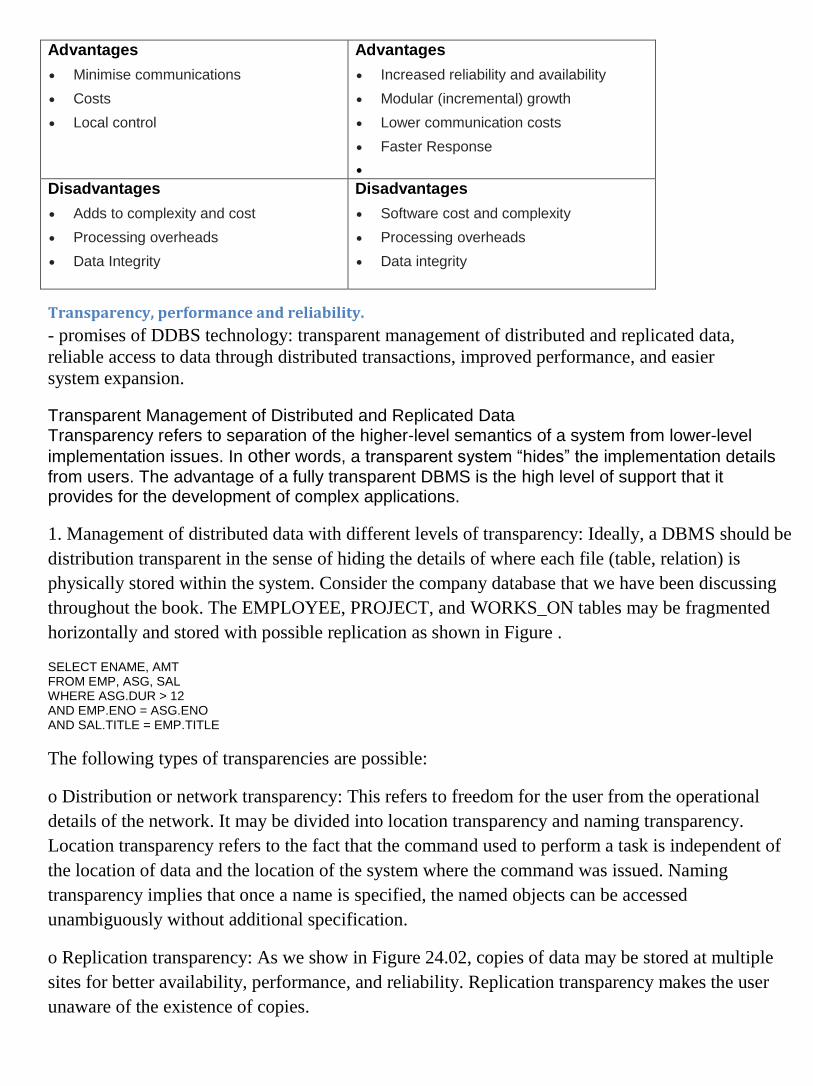
Advantages Minimise communications
Costs
Local control
Advantages Increased reliability and availability
Modular (incremental) growth
Lower communication costs
Faster Response
Disadvantages Adds to complexity and cost
Processing overheads
Data Integrity
Disadvantages Software cost and complexity
Processing overheads
Data integrity
Transparency, performance and reliability.
- promises of DDBS technology: transparent management of distributed and replicated data,
reliable access to data through distributed transactions, improved performance, and easier
system expansion.
Transparent Management of Distributed and Replicated Data Transparency refers to separation of the higher-level semantics of a system from lower-level
implementation issues. In other words, a transparent system “hides” the implementation details
from users. The advantage of a fully transparent DBMS is the high level of support that it provides for the development of complex applications.
1. Management of distributed data with different levels of transparency: Ideally, a DBMS should be
distribution transparent in the sense of hiding the details of where each file (table, relation) is
physically stored within the system. Consider the company database that we have been discussing
throughout the book. The EMPLOYEE, PROJECT, and WORKS_ON tables may be fragmented
horizontally and stored with possible replication as shown in Figure .
SELECT ENAME, AMT FROM EMP, ASG, SAL WHERE ASG.DUR > 12 AND EMP.ENO = ASG.ENO AND SAL.TITLE = EMP.TITLE
The following types of transparencies are possible:
o Distribution or network transparency: This refers to freedom for the user from the operational
details of the network. It may be divided into location transparency and naming transparency.
Location transparency refers to the fact that the command used to perform a task is independent of
the location of data and the location of the system where the command was issued. Naming
transparency implies that once a name is specified, the named objects can be accessed
unambiguously without additional specification.
o Replication transparency: As we show in Figure 24.02, copies of data may be stored at multiple
sites for better availability, performance, and reliability. Replication transparency makes the user
unaware of the existence of copies.
o Fragmentation transparency: Two types of fragmentation are possible. Horizontal fragmentation
distributes a relation into sets of tuples (rows). Vertical fragmentation distributes a relation into
subrelations where each subrelation is defined by a subset of the columns of the original relation. A
global query by the user must be transformed into several fragment queries. Fragmentation
transparency makes the user unaware of the existence of fragments.
2. Increased reliability and availability: These are two of the most common potential advantages
cited for distributed databases. Reliability is broadly defined as the probability that a system is
running (not down) at a certain time point, whereas availability is the probability that the system is
continuously available during a time interval. When the data and DBMS software are distributed
over several sites, one site may fail while other sites continue to operate. Only the data and
software that exist at the failed site cannot be accessed. This improves both reliability and
availability. Further improvement is achieved by judiciously replicating data and software at more
than one site. In a centralized system, failure at a single site makes the whole system unavailable to
all users. In a distributed database, some of the data may be unreachable, but users may still be able
to access other parts of the database.
3. Improved performance: A distributed DBMS fragments the database by keeping the data closer
to where it is needed most. Data localization reduces the contention for CPU and I/O services and
simultaneously reduces access delays involved in wide area networks. When a large database is
distributed over multiple sites, smaller databases exist at each site. As a result, local queries and
transactions accessing data at a single site have better performance because of the smaller local
databases. In addition, each site has a smaller number of transactions executing than if all
transactions are submitted to a single centralized database. Moreover, interquery and intraquery
parallelism can be achieved by executing multiple queries at different sites, or by breaking up a
query into a number of subqueries that execute in parallel. This contributes to improved
performance.
4. Easier expansion: In a distributed environment, expansion of the system in terms of adding more
data, increasing database sizes, or adding more processors is much easier.
Additional Functions of Distributed Databases
Distribution leads to increased complexity in the system design and implementation. To achieve the
potential advantages listed previously, the DDBMS software must be able to provide the following
functions in addition to those of a centralized DBMS:
• Keeping track of data: The ability to keep track of the data distribution, fragmentation, and
replication by expanding the DDBMS catalog.
• Distributed query processing: The ability to access remote sites and transmit queries and data
among the various sites via a communication network.
• Distributed transaction management: The ability to devise execution strategies for queries and
transactions that access data from more than one site and to synchronize the access to distributed
data and maintain integrity of the overall database.
• Replicated data management: The ability to decide which copy of a replicated data item to access
and to maintain the consistency of copies of a replicated data item.
• Distributed database recovery: The ability to recover from individual site crashes and from new
types of failures such as the failure of a communication links.
• Security: Distributed transactions must be executed with the proper management of the security of
the data and the authorization/access privileges of users.
• Distributed directory (catalog) management: A directory contains information (metadata) about
data in the database. The directory may be global for the entire DDB, or local for each site. The
placement and distribution of the directory are design and policy issues.
Problem areas of Distributed Database. :
Following are the Problems Areas of Distributed database. :-
1) Distributed Concurrency Control: - Distributed Concurrency Control specifies that
synchronization of access to the distributed database such that the integrity of the database is maintained. To
maintain Concurrency in distributed database different locking techniques should used which is based on mutual
exclusion of access to data. Time stamping algorithm also used where transactions are executed in some order [1].
2) Distributed Deadlock Management :- In distributed database several users are request for
resources from the database if the resources are available at that time , then database grant the resources to that
user if not available the user has to wait until the resources are released by other user. Sometimes the users are
not released the resources are blocked by some other user. This situation is known as Deadlock. Distributed
Deadlock is manage using the different algorithm and techniques such avoidance and detection algorithm.
3) Replication Control: - Replication is a technique that only applies to distributed systems. A database is said to be
replicated if the entire database or a portion of it (a table, some tables, one or more fragments, etc.) is copied and
the copies are stored at different sites. The issue with having more than one copy of a database is maintaining the
mutual consistency of the copies—ensuring that all copies have identical schema and data content.
4) Operating Environment: - To Implement Distributed Database Environment a Specific
Operating System is requirement as per Organizational needs. Operating system plays and
important role for managing the distributed database. Some time Operating system is not supported for
Distributed database.
5) Transparent Management: - Transparent management of Data is one of the major problem area in Distributed
database. In Distributed database data is situated in multiple locations and number Distributed Database Problem
areas and Approaches of users are used that database. To maintain the integrity of database transparent
management of
data is important.
6) Security and privacy: - How to apply the security policies to the interdependent system is a great issue in
distributed system. Since distributed systems deal with sensitive data and information so the system must have a
strong security and privacy measurement. Protection of distributed system assets, including base resources,
storage, communications and user-interface I/O as well as higherlevel composites of these resources, like
processes, files, messages, display windows and more complex objects, are important issues in distributed system
7) Resource management: - In distributed systems, objects consisting of resources are located on different places.
Routing is an issue at the network layer of the distributed system and at the application layer. Resource
management in a distributed system will interact with its eterogeneous Nature.
Integrity Constraints in Distributed Databases.
1.2 Distributed Database Architectures: DBMS standardization. Architectural models for
Distributed DBMS – autonomy, distribution and heterogeneity. Distributed Database
architecture – Client/Server, Peer-to-Peer distributed systems, MDBS Architecture.
Distributed Catalog management.
Distributed Database Architectures: DBMS standardization. The architecture of a system defines its structure. This means that the components of the system are identified, the function of each component is specified, and the interrelationships and interactions among these components are defined. The specification of the architecture of a system requires identification of the various modules, with their interfaces and interrelationships, in terms of the data and control flow through the system.
Architecture: The architecture of a system defines its structure:
– the components of the system are identified;
– the function of each component is specified;
– the interrelationships and interactions among the components are defined.
• Applies both for computer systems as well as for software systems, e.g,
– division into modules, description of modules, etc.
– architecture of a computer
• There is a close relationship between the architecture of a system, standardisation efforts, and a reference
model.
Motivation for Standardization of DDBMS Architecture
Standardization:
The standardization efforts in databases developed reference models of DBMS.
• Reference Model: A conceptual framework whose purpose is to divide standardization
work into manageable pieces and to show at a general level how these pieces are
related to each other.
• A reference model can be thought of as an idealized architectural model of the system.
• Commercial systems might deviate from reference model, still they are useful for the
standardization process
• A reference model can be described according to 3 different approaches:
– component-based
– function-based
– data-based
Components-based
– Components of the system are defined together with the interrelationships between the
components
– Good for design and implementation of the system
– It might be difficult to determine the functionality of the system from its components
Function-based
– Classes of users are identified together with the functionality that the system will provide
for each class
– Typically a hierarchical system with clearly defined interfaces between different layers
– The objectives of the system are clearly identified.
– Not clear how to achieve the objectives
– Example: ISO/OSI architecture of computer networks
Data-based
– Identify the different types of the data and specify the functional units that will realize
and/or use data according to these views
– Gives central importance to data (which is also the central resource of any DBMS)
!Claimed to be the preferable choice for standardization of DBMS
– The full architecture of the system is not clear without the description of functional
modules.
– Example: ANSI/SPARC architecture of DBMS
The interplay among the 3 approaches is important:
– Need to be used together to define an architectural model
– Each brings a different point of view and serves to focus on different aspects of the
model
In a homogeneous distributed database, all the sites use identical DBMS and operating systems. Its properties are:
The sites use very similar software.
The sites use identical DBMS or DBMS from the same vendor. Each site is aware of all other sites and cooperates with other sites to process user requests.
The database is accessed through a single interface as if it is a single database.

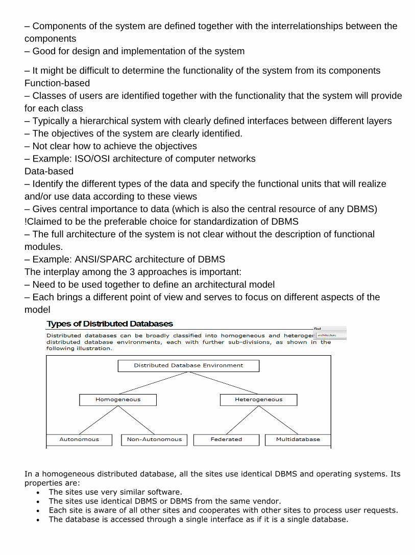
Types of Homogeneous Distributed Database There are two types of homogeneous distributed database:
Autonomous: Each database is independent that functions on its own. They are integrated by a
controlling application and use message passing to share data updates.
Non-autonomous: Data is distributed across the homogeneous nodes and a central or master
DBMS co-ordinates data updates across the sites.
Heterogeneous Distributed Databases In a heterogeneous distributed database, different sites have different operating systems, DBMS products and data models. Its properties are:
schemas and software.
erarchical or object oriented.
lex due to dissimilar schemas. re.
A site may not be aware of other sites and so there is limited co-operation in processing user
requests.
Types of Heterogeneous Distributed Databases: Federated: The heterogeneous database systems are independent in nature and integrated
together so that they function as a single database system.
Un-federated: The database systems employ a central coordinating module through which the
databases are accessed.
ANSI/SPARC architecture is based on data
3 views of data: external view, conceptual view, internal view
Defines a total of 43 interfaces between these views
Conceptual schema: Provides enterprise view of entire database RELATION EMP [
KEY = {ENO}
ATTRIBUTES = {
ENO : CHARACTER(9)
ENAME: CHARACTER(15)
TITLE: CHARACTER(10)
}
]
RELATION PAY [
KEY = {TITLE}
ATTRIBUTES = {
TITLE: CHARACTER(10)
SAL : NUMERIC(6)
RELATION PROJ [
KEY = {PNO}
ATTRIBUTES = {
PNO : CHARACTER(7)
PNAME :
CHARACTER(20)
BUDGET: NUMERIC(7)
LOC : CHARACTER(15)
}
]
RELATION ASG [
KEY = {ENO,PNO}
ATTRIBUTES = {
ENO : CHARACTER(9)
PNO : CHARACTER(7)
RESP: CHARACTER(10)
DUR : NUMERIC(3)
}
]

}
]
Internal schema: Describes the storage details of the relations.
– Relation EMP is stored on an indexed file
– Index is defined on the key attribute ENO and is called EMINX
– A HEADER field is used that might contain flags (delete, update, etc.) INTERNAL REL EMPL [
INDEX ON E# CALL EMINX
FIELD =
HEADER: BYTE(1)
E# : BYTE(9)
ENAME : BYTE(15)
TIT : BYTE(10)
]
External view: Specifies the view of different users/applications
– Application 1: Calculates the payroll payments for engineers CREATE VIEW PAYROLL (ENO, ENAME, SAL) AS
SELECT EMP.ENO,EMP.ENAME,PAY.SAL
FROM EMP, PAY
WHERE EMP.TITLE = PAY.TITLE
– Application 2: Produces a report on the budget of each project
CREATE VIEW BUDGET(PNAME, BUD) AS
SELECT PNAME, BUDGET
FROM PROJ
Architectural models for Distributed DBMS – autonomy, distribution and heterogeneity.
Architectural Models for DDBMSs (or more generally for multiple DBMSs) can be
classified along three dimensions:
– Autonomy
– Distribution
– Heterogeneity
Autonomy: Refers to the distribution of control (not of data) and indicates the degree to
which individual DBMSs can operate independently.
– Tight integration: a single-image of the entire database is available to any user who
wants to share the information (which may reside in multiple DBs); realized such that
one data manager is in control of the processing of each user request.
– Semiautonomous systems: individual DBMSs can operate independently, but have
decided to participate in a federation to make some of their local data sharable.
– Total isolation: the individual systems are stand-alone DBMSs, which know neither of
the existence of other DBMSs nor how to comunicate with them; there is no global
control.
• Autonomy has different dimensions
– Design autonomy: each individual DBMS is free to use the data models and
transaction management techniques that it prefers.
– Communication autonomy: each individual DBMS is free to decide what information
to provide to the other DBMSs
Conceptual schema:
RELATION EMP [
KEY = {ENO}
ATTRIBUTES = {
ENO : CHARACTER(9)
ENAME: CHARACTER(15)
TITLE: CHARACTER(10)
}
]

– Execution autonomy: each individual DBMS can execture the transactions that are
submitted to it in any way that it wants to.
Distribution: Refers to the physical distribution of data over multiple sites.
– No distribution: No distribution of data at all
Client/Server distribution:
_ Data are concentrated on the server, while clients provide application
environment/user interface
_ First attempt to distribution
–Peer-to-peer distribution (also called full distribution):
_ No distinction between client and server machine
_ Each machine has full DBMS functionality
Heterogeneity: Refers to heterogeneity of the components at various levels
– hardware
– communications
– operating system
– DB components (e.g., data model, query language, transaction management
algorithms)
Distributed Database architecture – Client/Server, Peer-to-Peer distributed systems, MDBS
Architecture.
Client-Server Architecture for DDBMS (Data-based) General idea: Divide the functionality into two classes:
*server functions - mainly data management, including query processing, optimization, transaction
management, etc.
*client functions
- might also include some data management functions (consistency checking, transaction
management, etc.) not just user interface
• Provides a two-level architecture
• More efficient division of work
• Different types of client/server architecture
– Multiple client/single server

– Multiple client/multiple server
Peer-to-Peer Architecture for DDBMS (Data-based)
Local internal schema (LIS)
– Describes the local physical data organization (which might be different
on each machine)

• Local conceptual schema (LCS)
– Describes logical data organization at each site
– Required since the data are fragmented and replicated
• Global conceptual schema (GCS)
– Describes the global logical view of the data
– Union of the LCSs
• External schema (ES)
– Describes the user/application view on the data
Multi-DBMS Architecture (Data-based)
Fundamental difference to peer-to-peer DBMS is in the definition of the global
conceptual schema (GCS)
– In a MDBMS the GCS represents only the collection of some of the local databases
that each local DBMS want to share.
• This leads to the question, whether the GCS should even exist in a MDBMS?
• Two different architecutre models:
– Models with a GCS
– Models without GCS
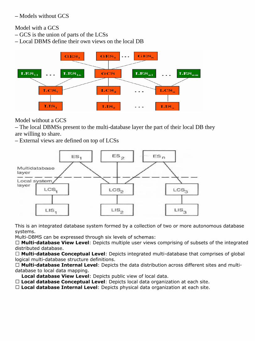
Model with a GCS
– GCS is the union of parts of the LCSs
– Local DBMS define their own views on the local DB
Model without a GCS
– The local DBMSs present to the multi-database layer the part of their local DB they
are willing to share.
– External views are defined on top of LCSs
This is an integrated database system formed by a collection of two or more autonomous database
systems. Multi-DBMS can be expressed through six levels of schemas:
Multi-database View Level: Depicts multiple user views comprising of subsets of the integrated
distributed database. Multi-database Conceptual Level: Depicts integrated multi-database that comprises of global
logical multi-database structure definitions. Multi-database Internal Level: Depicts the data distribution across different sites and multi-
database to local data mapping.
Local database View Level: Depicts public view of local data. Local database Conceptual Level: Depicts local data organization at each site.
Local database Internal Level: Depicts physical data organization at each site.
Distributed Catalog management.
1.3 Distributed Database Design: Design strategies and issues. Data Replication. Data
Fragmentation – Horizontal, Vertical and Mixed. Resource allocation. Semantic Data
Control in Distributed DBMS.
Distributed Database Design: Design strategies and issues.
Design Problem
• Design problem of distributed systems: Making decisions about the placement of data and
programs across the sites of a computer network as well as possibly designing the network itself.
• In DDBMS, the distribution of applications involves
– Distribution of the DDBMS software
– Distribution of applications that run on the database
• Distribution of applications will not be considered in the following; instead the distribution of
data is studied.
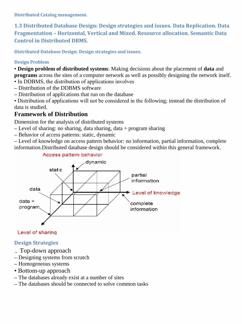
Framework of Distribution
Dimension for the analysis of distributed systems
– Level of sharing: no sharing, data sharing, data + program sharing
– Behavior of access patterns: static, dynamic
– Level of knowledge on access pattern behavior: no information, partial information, complete
information.Distributed database design should be considered within this general framework.
Design Strategies
Top-down approach – Designing systems from scratch
– Homogeneous systems
• Bottom-up approach – The databases already exist at a number of sites
– The databases should be connected to solve common tasks

Fig: Top-Down Design Process
Fig: Bottom-Up Design Process
Distribution design is the central part of the design in DDBMSs (the other tasks are similar to traditional databases)
– Objective: Design the LCSs by distributing the entities (relations) over the sites
– Two main aspects have to be designed carefully
∗ Fragmentation
· Relation may be divided into a number of sub-relations, which are distributed
∗ Allocation and replication
· Each fragment is stored at site with ”optimal” distribution
· Copy of fragment may be maintained at several sites
Distribution Design Issues
The following set of interrelated questions covers the entire issue. We will therefore

seek to answer them in the remainder of this section. 1. Why fragment at all? 2. How should we fragment? 3. How much should we fragment? 4. Is there any way to test the correctness of decomposition? 5. How should we allocate? 6. What is the necessary information for fragmentation and allocation?
Data Replication. Data Fragmentation – Horizontal, Vertical and Mixed.
What is a reasonable unit of distribution? Relation or fragment of relation?
• Relations as unit of distribution:
– If the relation is not replicated, we get a high volume of remote data accesses.
– If the relation is replicated, we get unnecessary replications, which cause problems in
executing updates and waste disk space
– Might be an Ok solution, if queries need all the data in the relation and data stays at
the only sites that uses the data
• Fragments of relationas as unit of distribution:
– Application views are usually subsets of relations
– Thus, locality of accesses of applications is defined on subsets of relations
– Permits a number of transactions to execute concurrently, since they will access
different portions of a relation
– Parallel execution of a single query (intra-query concurrency)
– However, semantic data control (especially integrity enforcement) is more difficult
⇒ Fragments of relations are (usually) the appropriate unit of distribution.
Fragmentation aims to improve:
– Reliability
– Performance
– Balanced storage capacity and costs
– Communication costs
– Security
• The following information is used to decide fragmentation:
– Quantitative information: frequency of queries, site, where query is run, selectivity of
the queries, etc.
– Qualitative information: types of access of data, read/write, etc.
Types of Fragmentation
– Horizontal: partitions a relation along its tuples
– Vertical: partitions a relation along its attributes
– Mixed/hybrid: a combination of horizontal and vertical fragmentation
a) Horizontal fragmentation
b) Vertical Fragmentation

c) Mixed Fragmentation
Example (contd.): Horizontal fragmentation of PROJ relation
– PROJ1: projects with budgets less than 200, 000
– PROJ2: projects with budgets greater than or equal to 200, 000
Correctness Rules of Fragmentation
Completeness
– Decomposition of relation R into fragments R1,R2, . . . ,Rn is complete iff each

data item in R can also be found in some Ri.
• Reconstruction
– If relation R is decomposed into fragments R1,R2, . . . ,Rn, then there should exist
some relational operator ∇ that reconstructs R from its fragments, i.e.,
R = R1∇. . .∇Rn
∗ Union to combine horizontal fragments
∗ Join to combine vertical fragments
• Disjointness
– If relation R is decomposed into fragments R1,R2, . . . ,Rn and data item di
appears in fragment Rj , then di should not appear in any other fragment Rk, k 6= j
(exception: primary key attribute for vertical fragmentation)
∗ For horizontal fragmentation, data item is a tuple
∗ For vertical fragmentation, data item is an attribute
Horizontal Fragmentation • Intuition behind horizontal fragmentation
– Every site should hold all information that is used to query at the site
– The information at the site should be fragmented so the queries of the site run faster
• Horizontal fragmentation is defined as selection operation, _p(R)
• Example:
_BUDGET<200000(PROJ)
_BUDGET≥200000(PROJ)
Computing horizontal fragmentation (idea)
– Compute the frequency of the individual queries of the site q1, . . . , qQ
– Rewrite the queries of the site in the conjunctive normal form (disjunction of
conjunctions); the conjunctions are called minterms.
– Compute the selectivity of the minterms
– Find the minimal and complete set of minterms (predicates)
∗ The set of predicates is complete if and only if any two tuples in the same fragment
are referenced with the same probability by any application
∗ The set of predicates is minimal if and only if there is at least one query that
accesses the fragment
– There is an algorithm how to find these fragments algorithmically (the algorithm
CON MIN and PHORIZONTAL (pp 120-122) of the textbook of the course)
Example: Fragmentation of the PROJ relation
– Consider the following query: Find the name and budget of projects given their PNO.
– The query is issued at all three sites
– Fragmentation based on LOC, using the set of predicates/minterms
{LOC =′ Montreal′,LOC =′ NewY ork′,LOC =′ Paris′}

If access is only according to the location, the above set of predicates is complete
– i.e., each tuple of each fragment PROJi has the same probability of being accessed
• If there is a second query/application to access only those project tuples where the
budget is less than $200000, the set of predicates is not complete.
– P2 in PROJ2 has higher probability to be accessed
Example (contd.):
– Add BUDGET ≤ 200000 and BUDGET > 200000 to the set of predicates
to make it complete.
⇒ {LOC =′ Montreal′,LOC =′ NewY ork′,LOC =′ Paris′,
BUDGET ≥ 200000,BUDGET < 200000} is a complete set
– Minterms to fragment the relation are given as follows:
(LOC =′ Montreal′) ∧ (BUDGET ≤ 200000)
(LOC =′ Montreal′) ∧ (BUDGET > 200000)
(LOC =′ NewY ork′) ∧ (BUDGET ≤ 200000)
(LOC =′ NewY ork′) ∧ (BUDGET > 200000)
(LOC =′ Paris′) ∧ (BUDGET ≤ 200000)
(LOC =′ Paris′) ∧ (BUDGET > 200000)
Vertical Fragmentation
Objective of vertical fragmentation is to partition a relation into a set of smaller relations
so that many of the applications will run on only one fragment.
• Vertical fragmentation of a relation R produces fragments R1,R2, . . . , each of which
contains a subset of R’s attributes.
• Vertical fragmentation is defined using the projection operation of the relational
algebra:
• Vertical fragmentation has also been studied for (centralized) DBMS
– Smaller relations, and hence less page accesses
– e.g., MONET system

Vertical fragmentation is inherently more complicated than horizontal fragmentation
– In horizontal partitioning: for n simple predicates, the number of possible minterms is
2n; some of them can be ruled out by existing implications/constraints.
– In vertical partitioning: for m non-primary key attributes, the number of possible
fragments is equal to B(m) (= the mth Bell number), i.e., the number of partitions of
a set with m members.
∗ For large numbers, B(m) ≈ mm (e.g., B(15) = 109)
• Optimal solutions are not feasible, and heuristics need to be applied.
Two types of heuristics for vertical fragmentation exist:
– Grouping: assign each attribute to one fragment, and at each step, join some of the
fragments until some criteria is satisfied.
∗ Bottom-up approach
– Splitting: starts with a relation and decides on beneficial partitionings based on the
access behaviour of applications to the attributes.
∗ Top-down approach
∗ Results in non-overlapping fragments
∗ “Optimal” solution is probably closer to the full relation than to a set of small
relations with only one attribute
∗ Only vertical fragmentation is considered here
DDB
Application information: The major information required as input for vertical
fragmentation is related to applications
– Since vertical fragmentation places in one fragment those attributes usually accessed
together, there is a need for some measure that would define more precisely the
notion of “togetherness”, i.e., how closely related the attributes are.
– This information is obtained from queries and collected in the Attribute Usage Matrix
and Attribute Affinity Matrix.
Given are the user queries/applications Q = (q1, . . . , qq) that will run on relation
R(A1, . . . ,An)
• Attribute Usage Matrix: Denotes which query uses which attribute:
use(qi,Aj) =( 1 iff qi uses Aj
0 otherwise
– The use(qi, •) vectors for each application are easy to define if the designer knows
the applications that willl run on the DB (consider also the 80-20 rule)
Example: Consider the following relation:
PROJ(PNO, PNAME,BUDGET,LOC)
and the following queries:
q1 = SELECT BUDGET FROM PROJ WHERE PNO=Value
q2 = SELECT PNAME,BUDGET FROM PROJ
q3 = SELECT PNAME FROM PROJ WHERE LOC=Value
q4 = SELECT SUM(BUDGET) FROM PROJ WHERE LOC =Value
• Lets abbreviate A1 = PNO,A2 = PNAME,A3 = BUDGET,A4 = LOC
• Attribute Usage Matrix
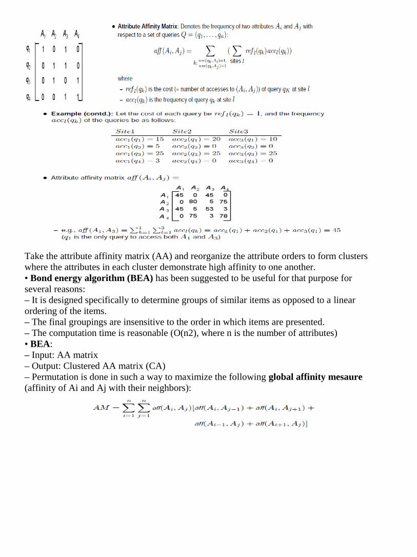
Take the attribute affinity matrix (AA) and reorganize the attribute orders to form clusters
where the attributes in each cluster demonstrate high affinity to one another.
• Bond energy algorithm (BEA) has been suggested to be useful for that purpose for
several reasons:
– It is designed specifically to determine groups of similar items as opposed to a linear
ordering of the items.
– The final groupings are insensitive to the order in which items are presented.
– The computation time is reasonable (O(n2), where n is the number of attributes)
• BEA:
– Input: AA matrix
– Output: Clustered AA matrix (CA)
– Permutation is done in such a way to maximize the following global affinity mesaure
(affinity of Ai and Aj with their neighbors):
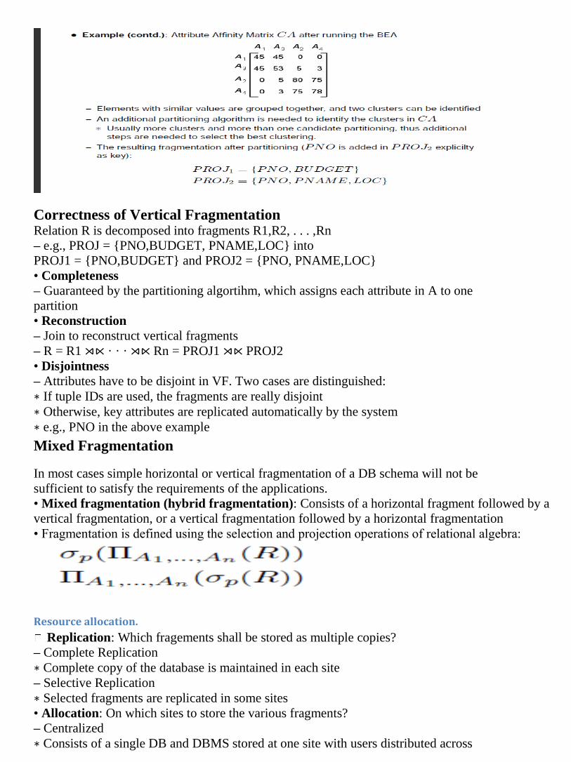
Correctness of Vertical Fragmentation Relation R is decomposed into fragments R1,R2, . . . ,Rn
– e.g., PROJ = {PNO,BUDGET, PNAME,LOC} into
PROJ1 = {PNO,BUDGET} and PROJ2 = {PNO, PNAME,LOC}
• Completeness
– Guaranteed by the partitioning algortihm, which assigns each attribute in A to one
partition
• Reconstruction
– Join to reconstruct vertical fragments
– R = R1 ⋊⋉ · · · ⋊⋉ Rn = PROJ1 ⋊⋉ PROJ2
• Disjointness
– Attributes have to be disjoint in VF. Two cases are distinguished:
∗ If tuple IDs are used, the fragments are really disjoint
∗ Otherwise, key attributes are replicated automatically by the system
∗ e.g., PNO in the above example
Mixed Fragmentation
In most cases simple horizontal or vertical fragmentation of a DB schema will not be
sufficient to satisfy the requirements of the applications.
• Mixed fragmentation (hybrid fragmentation): Consists of a horizontal fragment followed by a
vertical fragmentation, or a vertical fragmentation followed by a horizontal fragmentation
• Fragmentation is defined using the selection and projection operations of relational algebra:
Resource allocation.
Replication: Which fragements shall be stored as multiple copies?
– Complete Replication
∗ Complete copy of the database is maintained in each site
– Selective Replication
∗ Selected fragments are replicated in some sites
• Allocation: On which sites to store the various fragments?
– Centralized
∗ Consists of a single DB and DBMS stored at one site with users distributed across

the network
– Partitioned
∗ Database is partitioned into disjoint fragments, each fragment assigned to one site
Replication
Fragment Allocation
Fragment allocation problem
– Given are:
– fragments F = {F1, F2, ..., Fn}
– network sites S = {S1, S2, ..., Sm}
– and applications Q = {q1, q2, ..., ql}
– Find: the ”optimal” distribution of F to S
• Optimality
– Minimal cost
∗ Communication + storage + processing (read and update)
∗ Cost in terms of time (usually)
– Performance
∗ Response time and/or throughput
– Constraints
∗ Per site constraints (storage and processing)
Required information
– Database Information
∗ selectivity of fragments
∗ size of a fragment

– Application Information
∗ RRij : number of read accesses of a query qi to a fragment Fj
∗ URij : number of update accesses of query qi to a fragment Fj
∗ uij : a matrix indicating which queries updates which fragments,
∗ rij : a similar matrix for retrievals
∗ originating site of each query
– Site Information
∗ USCk: unit cost of storing data at a site Sk
∗ LPCk: cost of processing one unit of data at a site Sk
– Network Information
∗ communication cost/frame between two sites
∗ frame size
We present an allocation model which attempts to
– minimize the total cost of processing and storage
– meet certain response time restrictions
• General Form:
min(Total Cost)
– subject to
∗ response time constraint
∗ storage constraint
∗ processing constraint
• Functions for the total cost and the constraints are presented in the next slides.
• Decision variable xij
xij =( 1 if fragment Fi is stored at site Sj
0 otherwise

Solution Methods
– The complexity of this allocation model/problem is NP-complete
– Correspondence between the allocation problem and similar problems in other areas
∗ Plant location problem in operations research
∗ Knapsack problem
∗ Network flow problem
– Hence, solutions from these areas can be re-used
– Use different heuristics to reduce the search space
∗ Assume that all candidate partitionings have been determined together with their
associated costs and benefits in terms of query processing.
· The problem is then reduced to find the optimal partitioning and placement for
each relation
∗ Ignore replication at the first step and find an optimal non-replicated solution
· Replication is then handeled in a second step on top of the previous
non-replicated solution.
Semantic Data Control in Distributed DBMS.
Semantic Data Control
Semantic data control typically includes view management, security control, and
semantic integrity control.
• Informally, these functions must ensure that authorized users perform correct
operations on the database, contributing to the maintenance of database integrity.
• In RDBMS semantic data control can be achieved in a uniform way
– views, security constraints, and semantic integrity constraints can be defined as rules
that the system automatically enforces
View Management
Views enable full logical data independence
• Views are virtual relations that are defined as the result of a query on base relations
• Views are typically not materialized
– Can be considered a dynamic window that reflects all relevant updates to the
database
• Views are very useful for ensuring data security in a simple way
– By selecting a subset of the database, views hide some data
– Users cannot see the hidden data
View Management in Distributed Databases
• Definition of views in DDBMS is similar as in centralized DBMS
– However, a view in a DDBMS may be derived from fragmented relations stored at
different sites
• Views are conceptually the same as the base relations, therefore we store them in the
(possibly) distributed directory/catalogue
– Thus, views might be centralized at one site, partially replicated, fully replicated
– Queries on views are translated into queries on base relations, yielding distributed
queries due to possible fragmentation of data
• Views derived from distributed relations may be costly to evaluate
– Optimizations are important, e.g., snapshots
– A snapshot is a static view
∗ does not reflect the updates to the base relations
∗ managed as temporary relations: the only access path is sequential scan
∗ typically used when selectivity is small (no indices can be used efficiently)
∗ is subject to periodic recalculation
Data Security
Data security protects data against unauthorized acces and has two aspects:

– Data protection
– Authorization control
Data Protection
Data protection prevents unauthorized users from understanding the physical content of data.
• Well established standards exist
– Data encryption standard
– Public-key encryption schemes
Authorization Control
Authorization control must guarantee that only authorized users perform operations
they are allowed to perform on the database.
• Three actors are involved in authorization
– users, who trigger the execution of application programms
– operations, which are embedded in applications programs
– database objects, on which the operations are performed
• Authorization control can be viewed as a triple (user, operation type, object) which specifies that
the user has the right to perform an operation of operation type on an object.
• Authentication of (groups of) users is typically done by username and password
• Authorization control in (D)DBMS is more complicated as in operating systems
– In a file system: data objects are files
– In a DBMS: Data objects are views, (fragments of) relations, tuples, attributes
Semantic Integrity Constraints
A database is said to be consistent if it satisfies a set of constraints, called semantic
integrity constraints
• Maintain a database consistent by enforcing a set of constraints is a difficult problem
• Semantic integrity control evolved from procedural methods (in which the controls were
embedded in application programs) to declarative methods
– avoid data dependency problem, code redundancy, and poor performance of the
procedural methods
• Two main types of constraints can be distinguished:
– Structural constraints: basic semantic properties inherent to a data model e.g.,
unique key constraint in relational model
– Behavioral constraints: regulate application behavior e.g., dependencies
(functional, inclusion) in the relational model
• A semantic integrity control system has 2 components:
– Integrity constraint specification
– Integrity constraint enforcement
Integrity constraints specification
– In RDBMS, integrity constraints are defined as assertions, i.e., expression in tuple
relational calculus
– Variables are either universally (∀) or existentially (∃) quantified
– Declarative method
– Easy to define constraints
– Can be seen as a query qualification which is either true or false
– Definition of database consistency clear
– 3 types of integrity constraints/assertions are distinguished:
∗ predefined
∗ precompiled
∗ general constraints
• In the following examples we use the following relations:
EMP(ENO, ENAME, TITLE)
PROJ(PNO, PNAME, BUDGET)
ASG(ENO, PNO, RESP, DUR)
Predefined constraints are based on simple keywords and specify the more common
contraints of the relational model
• Not-null attribute:
– e.g., Employee number in EMP cannot be null
ENO NOT NULL IN EMP
• Unique key:
– e.g., the pair (ENO,PNO) is the unique key in ASG
(ENO, PNO) UNIQUE IN ASG
• Foreign key:
– e.g., PNO in ASG is a foreign key matching the primary key PNO in PROJ
PNO IN ASG REFERENCES PNO IN PROJ
• Functional dependency:
– e.g., employee number functionally determines the employee name
ENO IN EMP DETERMINES ENAME
Precompiled constraints express preconditions that must be satisfied by all tuples in a
relation for a given update type
• General form:
CHECK ON <relation> [WHEN <update type>] <qualification>
• Domain constraint, e.g., constrain the budget:
CHECK ON PROJ(BUDGET>500000 AND BUDGET≤1000000)
• Domain constraint on deletion, e.g., only tuples with budget 0 can be deleted:
CHECK ON PROJ WHEN DELETE (BUDGET = 0)
• Transition constraint, e.g., a budget can only increase:
CHECK ON PROJ (NEW.BUDGET > OLD.BUDGET AND
NEW.PNO = OLD.PNO)
– OLD and NEW are implicitly defined variables to identify the tuples that are subject to
Update
General constraints may involve more than one relation
• General form:
CHECK ON <variable>:<relation> (<qualification>)
• Functional dependency:
CHECK ON e1:EMP, e2:EMP
(e1.ENAME = e2.ENAME IF e1.ENO = e2.ENO)
• Constraint with aggregate function:
e.g., The total duration for all employees in the CAD project is less than 100

CHECK ON g:ASG, j:PROJ
( SUM(g.DUR WHERE g.PNO=j.PNO) < 100
IF j.PNAME="CAD/CAM" )
Semantic Integrity Constraints Enforcement
Enforcing semantic integrity constraints consists of rejecting update programs that
violate some integrity constraints
• Thereby, the major problem is to find efficient algorithms
• Two methods to enforce integrity constraints:
– Detection:
1. Execute update u : D → Du
2. If Du is inconsistent then compensate Du → D′
u or undo Du → D
∗ Also called posttest
∗ May be costly if undo is very large
– Prevention:
Execute u : D → Du only if Du will be consistent
∗ Also called pretest
∗ Generally more efficient
∗ Query modification algorithm by Stonebraker (1975) is a preventive method that is
particularly efficient in enforcing domain constraints.
· Add the assertion qualification (constraint) to the update query and check it
immediately for each tuple
Example: Consider a query for increasing the budget of CAD/CAM projects by 10%:
UPDATE PROJ
SET BUDGET = BUDGET * 1.1
WHERE PNAME = ‘‘CAD/CAM’’
and the domain constraint
CHECK ON PROJ (BUDGET >= 50K AND BUDGET <= 100K)
The query modification algorithm transforms the query into:
UPDATE PROJ
SET BUDGET = BUDGET * 1.1
WHERE PNAME = ‘‘CAD/CAM’’
AND NEW.BUDGET >= 50K
AND NEW.BUDGET <= 100K
Distributed Constraints
Three classes of distributed integrity constraints/assertions are distinguished:
– Individual assertions
∗ Single relation, single variable
∗ Refer only to tuples to be updated independenlty of the rest of the DB
∗ e.g., domain constraints
– Set-oriented assertions
∗ Single relation, multi variable (e.g., functional dependencies)
∗ Multi-relation, multi-variable (e.g., foreign key constraints)
∗ Multiple tuples form possibly different relations are involved
– Assertions involving aggregates
∗ Special, costly processing of aggregates is required
Particular difficulties with distributed constraints arise from the fact that relations are
fragmented and replicated:
– Definition of assertions
– Where to store the assertions?
– How to enforce the assertions?
Definition and storage of assertions
– The definition of a new integrity assertion can be started at one of the sites that store
the relations involved in the assertion, but needs to be propagated to sites that might
store fragments of that relation.
– Individual assertions
∗ The assertion definition is sent to all other sites that contain fragments of the
relation involved in the assertion.
∗ At each fragment site, check for compatibility of assertion with data
∗ If compatible, store; otherwise reject
∗ If any of the sites rejects, globally reject
– Set-oriented assertions
∗ Involves joins (between fragments or relations)
∗ Maybe necessary to perform joins to check for compatibility
∗ Store if compatible
Enforcement of assertions in DDBMS is more complex than in centralized DBMS
• The main problem is to decide where (at which site) to enforce each assertion?
– Depends on type of assertion, type of update, and where update is issued
• Individual assertions
– Update = insert
∗ enforce at the site where the update is issued (i.e., where the user inserts the
tuples)
– Update = delete or modify
∗ Send the assertions to all the sites involved (i.e., where qualified tuples are
updated)
∗ Each site enforce its own assertion
• Set-oriented assertions
– Single relation
∗ Similar to individual assertions with qualified updates
– Multi-relation
∗ Move data between sites to perform joins
∗ Then send the result to the query master site (the site the update is issued)
Unit 2: 17 hrs.
2.1 Distributed Query Processing: Query Decomposition and Data localization for
distributed data, join ordering, semi-join strategy, Distributed Query optimization
methods.
Distributed Query Processing: Query Decomposition and Data localization for distributed data,
Query Processing Overview:
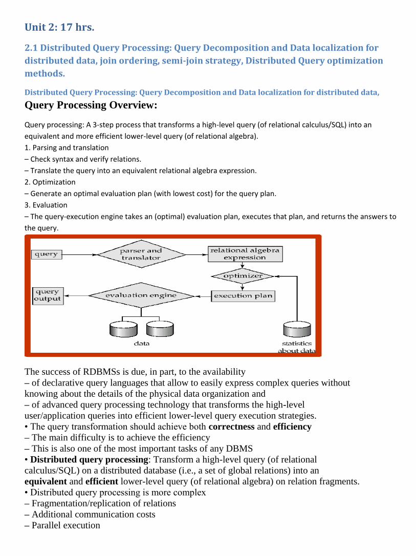
Query processing: A 3-step process that transforms a high-level query (of relational calculus/SQL) into an
equivalent and more efficient lower-level query (of relational algebra).
1. Parsing and translation
– Check syntax and verify relations.
– Translate the query into an equivalent relational algebra expression.
2. Optimization
– Generate an optimal evaluation plan (with lowest cost) for the query plan.
3. Evaluation
– The query-execution engine takes an (optimal) evaluation plan, executes that plan, and returns the answers to
the query.
The success of RDBMSs is due, in part, to the availability
– of declarative query languages that allow to easily express complex queries without
knowing about the details of the physical data organization and
– of advanced query processing technology that transforms the high-level
user/application queries into efficient lower-level query execution strategies.
• The query transformation should achieve both correctness and efficiency
– The main difficulty is to achieve the efficiency
– This is also one of the most important tasks of any DBMS
• Distributed query processing: Transform a high-level query (of relational
calculus/SQL) on a distributed database (i.e., a set of global relations) into an
equivalent and efficient lower-level query (of relational algebra) on relation fragments.
• Distributed query processing is more complex
– Fragmentation/replication of relations
– Additional communication costs
– Parallel execution
Query Optimization
Query optimization is a crucial and difficult part of the overall query processing
• Objective of query optimization is to minimize the following cost function:
I/O cost + CPU cost + communication cost
• Two different scenarios are considered:
– Wide area networks
Communication cost dominates
· low bandwidth
· low speed
· high protocol overhead
Most algorithms ignore all other cost components
– Local area networks
Communication cost not that dominant
Total cost function should be considered
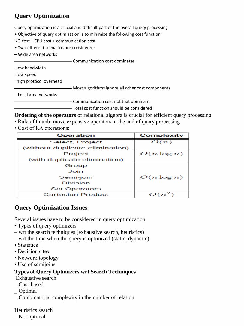
Ordering of the operators of relational algebra is crucial for efficient query processing
• Rule of thumb: move expensive operators at the end of query processing
• Cost of RA operations:
Query Optimization Issues
Several issues have to be considered in query optimization
• Types of query optimizers
– wrt the search techniques (exhaustive search, heuristics)
– wrt the time when the query is optimized (static, dynamic)
• Statistics
• Decision sites
• Network topology
• Use of semijoins
Types of Query Optimizers wrt Search Techniques
Exhaustive search
_ Cost-based
_ Optimal
_ Combinatorial complexity in the number of relation
Heuristics search
_ Not optimal
_ Regroups common sub-expressions
_ Performs selection, projection first
_ Replaces a join by a series of semijoins
_ Reorders operations to reduce intermediate relation size
_ Optimizes individual operations
Types of Query Optimizers wrt Optimization Timing
– Static
Query is optimized prior to the execution
As a consequence it is difficult to estimate the size of the intermediate
results
Typically amortizes over many executions
– Dynamic
Optimization is done at run time
Provides exact information on the intermediate relation sizes
Have to re-optimize for multiple executions
– Hybrid
First, the query is compiled using a static algorithm
Then, if the error in estimate sizes greater than threshold, the query is re-
optimized
at run time
** Statistics
– Relation/fragments
Cardinality
Size of a tuple
Fraction of tuples participating in a join with another relation/fragment
– Attribute
Cardinality of domain
Actual number of distinct values
Distribution of attribute values (e.g., histograms)
– Common assumptions
Independence between different attribute values
Uniform distribution of attribute values within their domain
**Decision sites
– Centralized
Single site determines the ”best” schedule
Simple
Knowledge about the entire distributed database is needed
– Distributed
Cooperation among sites to determine the schedule
Only local information is needed
Cooperation comes with an overhead cost
– Hybrid

One site determines the global schedule
Each site optimizes the local sub-queries
**Network topology
– Wide area networks (WAN) point-to-point
Characteristics
· Low bandwidth
· Low speed
· High protocol overhead
Communication cost dominate; all other cost factors are ignored
Global schedule to minimize communication cost
Local schedules according to centralized query optimization
– Local area networks (LAN)
Communication cost not that dominant
Total cost function should be considered
Broadcasting can be exploited (joins)
Special algorithms exist for star networks
**
Use of Semijoins
– Reduce the size of the join operands by first computing semijoins
– Particularly relevant when the main cost is the communication cost
– Improves the processing of distributed join operations by reducing the size of data
exchange between sites
– However, the number of messages as well as local processing time is increased
Query Decomposition
Query decomposition: Mapping of calculus query (SQL) to algebra operations (select, project, join, rename)
• Both input and output queries refer to global relations, without knowledge of the distribution of data.
• The output query is semantically correct and good in the sense that redundant work is avoided.
• Query decomposistion consists of 4 steps:
1. Normalization: Transform query to a normalized form
2. Analysis: Detect and reject ”incorrect” queries; possible only for a subset of relational calculus
3. Elimination of redundancy: Eliminate redundant predicates
4. Rewriting: Transform query to RA and optimize query
Normalization: Transform the query to a normalized form to facilitate further processing.
Consists mainly of two steps.
1. Lexical and syntactic analysis
– Check validity (similar to compilers)
– Check for attributes and relations
– Type checking on the qualification
2. Put into normal form
– With SQL, the query qualification (WHERE clause) is the most difficult part as it
might be an arbitrary complex predicate preceeded by quantifiers (9, 8)
– Conjunctive normal form
(p11 _ p12 _ · · · _ p1n) ^ · · · ^ (pm1 _ pm2 _ · · · _ pmn)
– Disjunctive normal form
(p11 ^ p12 ^ · · · ^ p1n) _ · · · _ (pm1 ^ pm2 ^ · · · ^ pmn)
– In the disjunctive normal form, the query can be processed as independent
conjunctive subqueries linked by unions (corresponding to the disjunction)
Example: Consider the following query: Find the names of employees who have been
working on project P1 for 12 or 24 months?
• The query in SQL:
SELECT ENAME
FROM EMP, ASG
WHERE EMP.ENO = ASG.ENO AND
ASG.PNO = ‘‘P1’’ AND
DUR = 12 OR DUR = 24
• The qualification in conjunctive normal form:
EMP.ENO = ASG.ENO ^ ASG.PNO = ”P1” ^ (DUR = 12 _ DUR = 24)
• The qualification in disjunctive normal form:
(EMP.ENO = ASG.ENO ^ ASG.PNO = ”P1” ^ DUR = 12) _
(EMP.ENO = ASG.ENO ^ ASG.PNO = ”P1” ^ DUR = 24)
Query Decomposition – Analysis
Analysis: Identify and reject type incorrect or semantically incorrect queries
• Type incorrect
– Checks whether the attributes and relation names of a query are defined in the global
schema
– Checks whether the operations on attributes do not conflict with the types of the
attributes, e.g., a comparison > operation with an attribute of type string
• Semantically incorrect
– Checks whether the components contribute in any way to the generation of the result
– Only a subset of relational calculus queries can be tested for correctness, i.e., those
that do not contain disjunction and negation
– Typical data structures used to detect the semantically incorrect queries are:
Connection graph (query graph)
Join graph
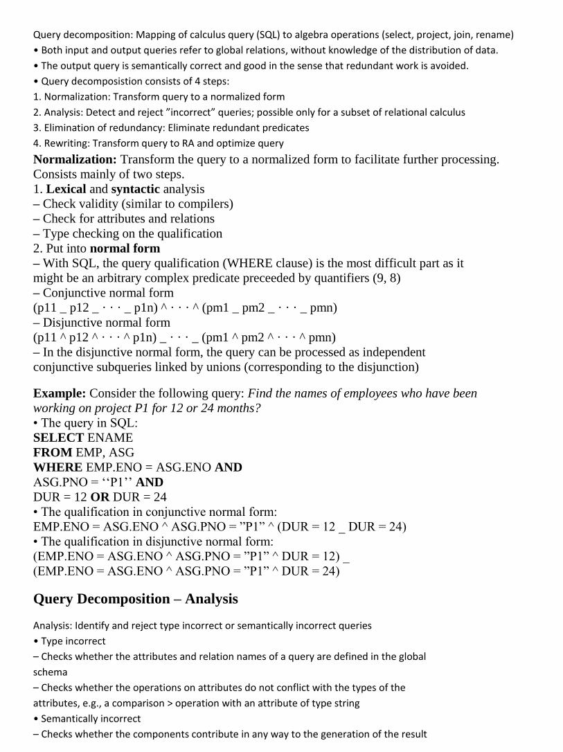
Example: Consider a query:
SELECT ENAME,RESP
FROM EMP, ASG, PROJ
WHERE EMP.ENO = ASG.ENO
AND ASG.PNO = PROJ.PNO
AND PNAME = "CAD/CAM"
AND DUR 36
AND TITLE = "Programmer"
• Query/connection graph
– Nodes represent operand or result relation
– Edge represents a join if both connected nodes represent an operand relation, otherwise it is a projection
• Join graph
– a subgraph of the query graph that considers only the joins
• Since the query graph is connected, the query is semantically correct
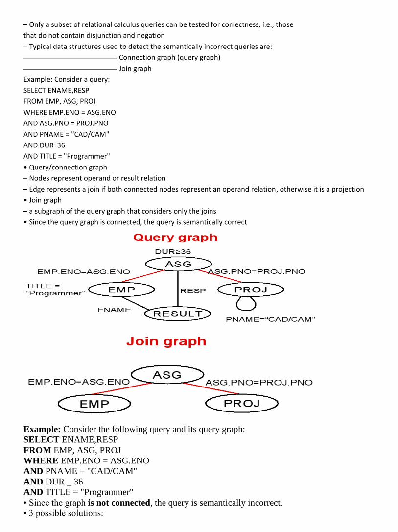
Example: Consider the following query and its query graph:
SELECT ENAME,RESP
FROM EMP, ASG, PROJ
WHERE EMP.ENO = ASG.ENO
AND PNAME = "CAD/CAM"
AND DUR _ 36
AND TITLE = "Programmer"
• Since the graph is not connected, the query is semantically incorrect.
• 3 possible solutions:
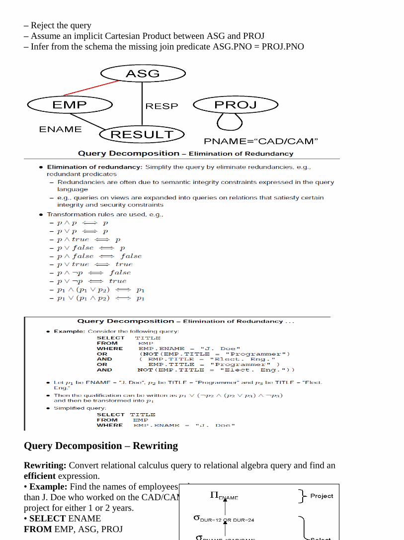
– Reject the query
– Assume an implicit Cartesian Product between ASG and PROJ
– Infer from the schema the missing join predicate ASG.PNO = PROJ.PNO
Query Decomposition – Rewriting
Rewriting: Convert relational calculus query to relational algebra query and find an
efficient expression.
• Example: Find the names of employees other
than J. Doe who worked on the CAD/CAM
project for either 1 or 2 years.
• SELECT ENAME
FROM EMP, ASG, PROJ
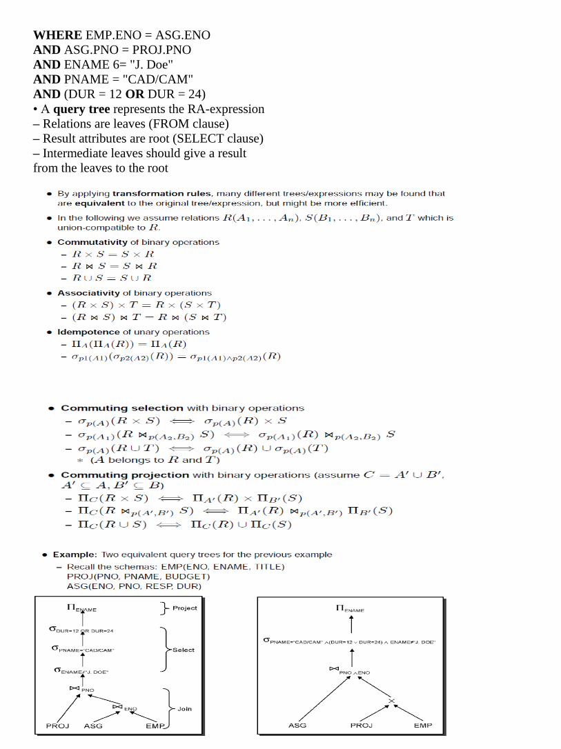
WHERE EMP.ENO = ASG.ENO
AND ASG.PNO = PROJ.PNO
AND ENAME 6= "J. Doe"
AND PNAME = "CAD/CAM"
AND (DUR = 12 OR DUR = 24)
• A query tree represents the RA-expression
– Relations are leaves (FROM clause)
– Result attributes are root (SELECT clause)
– Intermediate leaves should give a result
from the leaves to the root

Data Localization – Input: Algebraic query on global conceptual schema – Purpose: Apply data distribution information to the algebra operations and determine which
fragments are involved
_ Substitute global query with queries on fragments
_ Optimize the global query
Example (contd.): Parallelsim in the evaluation is often possible
– Depending on the horizontal fragmentation, the fragments can be joined in parallel
followed by the union of the intermediate results.
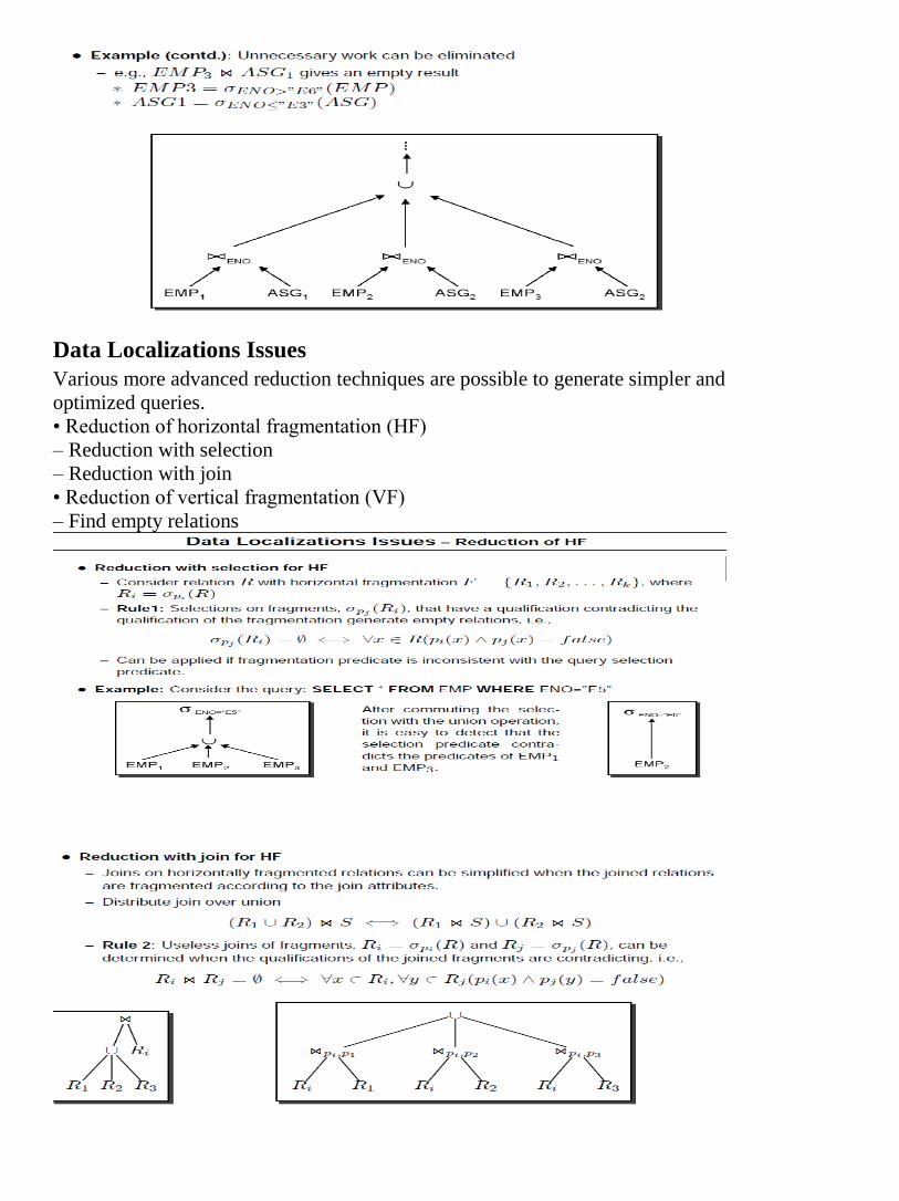
Data Localizations Issues
Various more advanced reduction techniques are possible to generate simpler and
optimized queries.
• Reduction of horizontal fragmentation (HF)
– Reduction with selection
– Reduction with join
• Reduction of vertical fragmentation (VF)
– Find empty relations

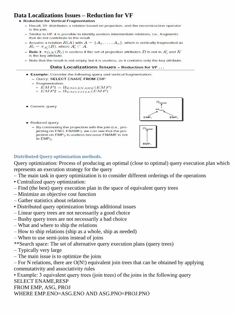
Data Localizations Issues – Reduction for VF
Distributed Query optimization methods.
Query optimization: Process of producing an optimal (close to optimal) query execution plan which
represents an execution strategy for the query
– The main task in query optimization is to consider different orderings of the operations
• Centralized query optimization:
– Find (the best) query execution plan in the space of equivalent query trees
– Minimize an objective cost function
– Gather statistics about relations
• Distributed query optimization brings additional issues
– Linear query trees are not necessarily a good choice
– Bushy query trees are not necessarily a bad choice
– What and where to ship the relations
– How to ship relations (ship as a whole, ship as needed)
– When to use semi-joins instead of joins
**Search space: The set of alternative query execution plans (query trees)
– Typically very large
– The main issue is to optimize the joins
– For N relations, there are O(N!) equivalent join trees that can be obtained by applying
commutativity and associativity rules
• Example: 3 equivalent query trees (join trees) of the joins in the following query
SELECT ENAME,RESP
FROM EMP, ASG, PROJ
WHERE EMP.ENO=ASG.ENO AND ASG.PNO=PROJ.PNO

join ordering,
Join ordering is an important aspect in centralized DBMS, and it is even more
important in a DDBMS since joins between fragments that are stored at different sites
may increase the communication time.
• Two approaches exist:
*Optimize the ordering of joins directly
_ INGRES and distributed INGRES
_ System R and System R∗
* Replace joins by combinations of semijoins in order to minimize the communication
costs
_ Hill Climbing and SDD-1
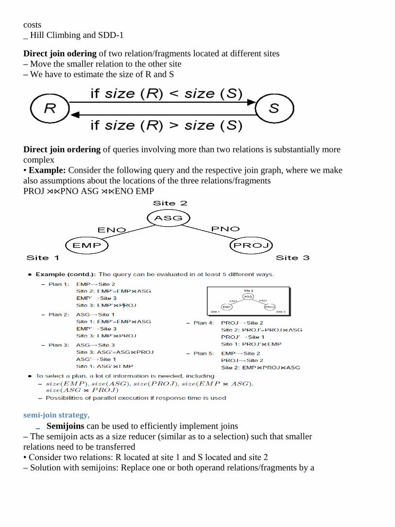
Direct join odering of two relation/fragments located at different sites
– Move the smaller relation to the other site
– We have to estimate the size of R and S
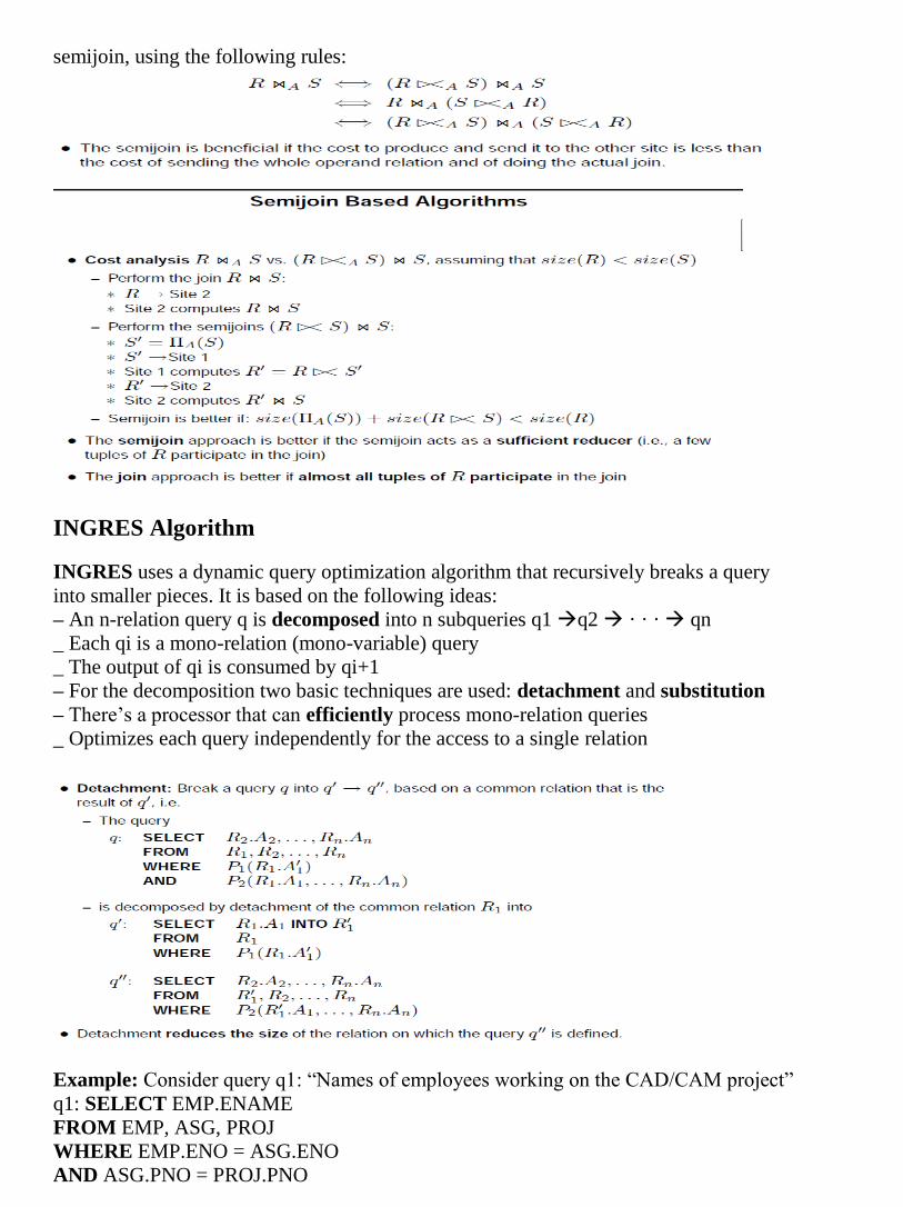
Direct join ordering of queries involving more than two relations is substantially more
complex
• Example: Consider the following query and the respective join graph, where we make
also assumptions about the locations of the three relations/fragments
PROJ ⋊⋉PNO ASG ⋊⋉ENO EMP
semi-join strategy,
Semijoins can be used to efficiently implement joins
– The semijoin acts as a size reducer (similar as to a selection) such that smaller
relations need to be transferred
• Consider two relations: R located at site 1 and S located and site 2
– Solution with semijoins: Replace one or both operand relations/fragments by a
semijoin, using the following rules:
INGRES Algorithm
INGRES uses a dynamic query optimization algorithm that recursively breaks a query
into smaller pieces. It is based on the following ideas:
– An n-relation query q is decomposed into n subqueries q1 q2 · · · qn
_ Each qi is a mono-relation (mono-variable) query
_ The output of qi is consumed by qi+1
– For the decomposition two basic techniques are used: detachment and substitution
– There’s a processor that can efficiently process mono-relation queries
_ Optimizes each query independently for the access to a single relation
Example: Consider query q1: “Names of employees working on the CAD/CAM project”
q1: SELECT EMP.ENAME
FROM EMP, ASG, PROJ
WHERE EMP.ENO = ASG.ENO
AND ASG.PNO = PROJ.PNO
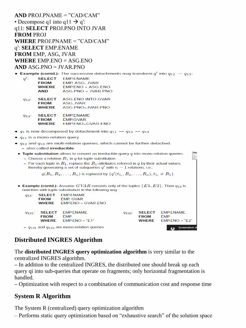
AND PROJ.PNAME = ”CAD/CAM”
• Decompose q1 into q11 q′:
q11: SELECT PROJ.PNO INTO JVAR
FROM PROJ
WHERE PROJ.PNAME = ”CAD/CAM”
q′: SELECT EMP.ENAME
FROM EMP, ASG, JVAR
WHERE EMP.ENO = ASG.ENO
AND ASG.PNO = JVAR.PNO
Distributed INGRES Algorithm
The distributed INGRES query optimization algorithm is very similar to the
centralized INGRES algorithm.
– In addition to the centralized INGRES, the distributed one should break up each
query qi into sub-queries that operate on fragments; only horizontal fragmentation is
handled.
– Optimization with respect to a combination of communication cost and response time
System R Algorithm
The System R (centralized) query optimization algorithm
– Performs static query optimization based on “exhaustive search” of the solution space
and a cost function (IO cost + CPU cost)
Input: relational algebra tree
Output: optimal relational algebra tree
Dynamic programming technique is applied to reduce the number of
alternative
plans
– The optimization algorithm consists of two steps
1. Predict the best access method to each individual relation (mono-relation query)
Consider using index, file scan, etc.
2. For each relation R, estimate the best join ordering
R is first accessed using its best single-relation access method
Efficient access to inner relation is crucial
– Considers two different join strategies
(Indexed-) nested loop join
Sort-merge join
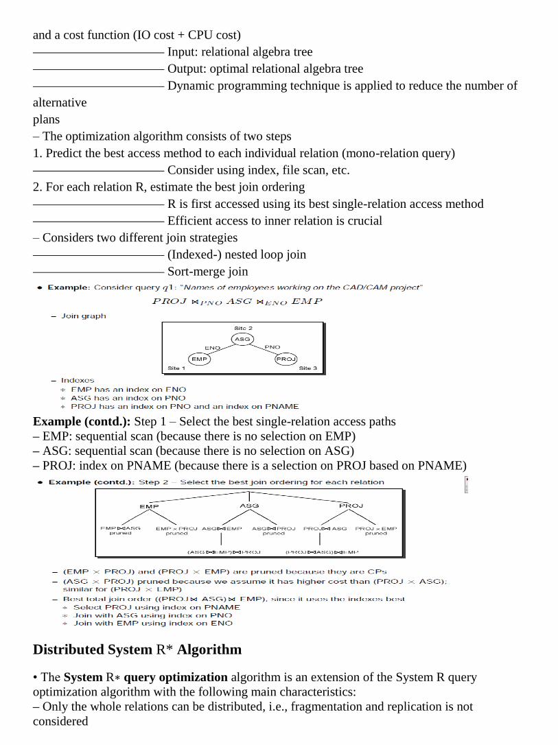
Example (contd.): Step 1 – Select the best single-relation access paths
– EMP: sequential scan (because there is no selection on EMP)
– ASG: sequential scan (because there is no selection on ASG)
– PROJ: index on PNAME (because there is a selection on PROJ based on PNAME)
Distributed System R* Algorithm
• The System R∗ query optimization algorithm is an extension of the System R query
optimization algorithm with the following main characteristics:
– Only the whole relations can be distributed, i.e., fragmentation and replication is not
considered
– Query compilation is a distributed task, coordinated by a master site, where the
query is initiated
– Master site makes all inter-site decisions, e.g., selection of the execution sites, join
ordering, method of data transfer, ...
– The local sites do the intra-site (local) optimizations, e.g., local joins, access paths
• Join ordering and data transfer between different sites are the most critical issues to be
considered by the master site
Two methods for inter-site data transfer
– Ship whole: The entire relation is shipped to the join site and stored in a temporary
relation
Larger data transfer
Smaller number of messages
Better if relations are small
– Fetch as needed: The external relation is sequentially scanned, and for each tuple
the join value is sent to the site of the inner relation and the matching inner tuples are
sent back (i.e., semijoin)
Number of messages = O(cardinality of outer relation)
Data transfer per message is minimal
Better if relations are large and the selectivity is good
Hill-Climbing Algorithm
Hill-Climbing query optimization algorithm
– Refinements of an initial feasible solution are recursively computed until no more cost
improvements can be made
– Semijoins, data replication, and fragmentation are not used
– Devised for wide area point-to-point networks
– The first distributed query processing algorithm
The hill-climbing algorithm proceeds as follows
1. Select initial feasible execution strategy ES0
– i.e., a global execution schedule that includes all intersite communication
– Determine the candidate result sites, where a relation referenced in the query exist
– Compute the cost of transferring all the other referenced relations to each
candidate site
– ES0 = candidate site with minimum cost
2. Split ES0 into two strategies: ES1 followed by ES2
– ES1: send one of the relations involved in the join to the other relation’s site
– ES2: send the join result to the final result site
3. Replace ES0 with the split schedule which gives
cost(ES1) + cost(local join) + cost(ES2) < cost(ES0)
4. Recursively apply steps 2 and 3 on ES1 and ES2 until no more benefit can be gained
5. Check for redundant transmissions in the final plan and eliminate them

SDD-1 The SDD-1 query optimization algorithm improves the Hill-Climbing algorithm in a
number of directions:
– Semijoins are considered
– More elaborate statistics
– Initial plan is selected better
– Post-optimization step is introduced
2.2 Distributed Transaction Management: The concept and role of transaction.
Properties of transactions-Atomicity, Consistency, Isolation and Durability.
Architectural aspects of Distributed Transaction, Transaction Serialization.
Distributed Transaction Management: The concept and role of transaction.
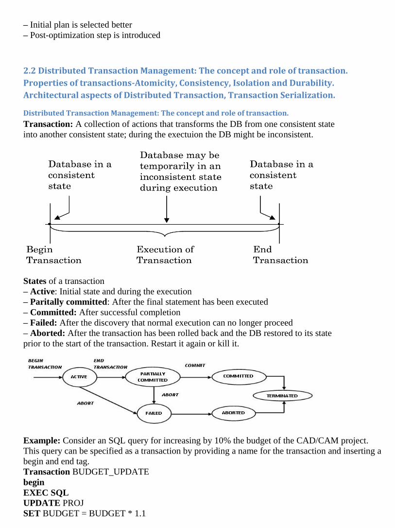
Transaction: A collection of actions that transforms the DB from one consistent state
into another consistent state; during the exectuion the DB might be inconsistent.
States of a transaction
– Active: Initial state and during the execution
– Paritally committed: After the final statement has been executed
– Committed: After successful completion
– Failed: After the discovery that normal execution can no longer proceed
– Aborted: After the transaction has been rolled back and the DB restored to its state
prior to the start of the transaction. Restart it again or kill it.
Example: Consider an SQL query for increasing by 10% the budget of the CAD/CAM project.
This query can be specified as a transaction by providing a name for the transaction and inserting a
begin and end tag.
Transaction BUDGET_UPDATE
begin
EXEC SQL
UPDATE PROJ
SET BUDGET = BUDGET * 1.1

WHERE PNAME = "CAD/CAM"
end.
Example: Consider an airline DB with the following relations:
FLIGHT(FNO, DATE, SRC, DEST, STSOLD, CAP)
CUST(CNAME, ADDR, BAL)
FC(FNO, DATE, CNAME, SPECIAL)
• Consider the reservation of a ticket, where a travel agent enters the flight number, the
date, and a customer name, and then asks for a reservation.
Begin transaction Reservation
begin
input(flight_no, date, customer_name);
EXEC SQL UPDATE FLIGHT
SET STSOLD = STSOLD + 1
WHERE FNO = flight_no AND DATE = date;
EXEC SQL INSERT
INTO FC(FNO, DATE, CNAME, SPECIAL);
VALUES (flight_no, date, customer_name, null);
output("reservation completed")
end.
Transactions are mainly characterized by its Read and Write operations
– Read set (RS): The data items that a transaction reads
– Write set (WS): The data items that a transaction writes
– Base set (BS): the union of the read set and write set
Formalization of a Transaction
We use the following notation:
– Ti be a transaction and x be a relation or a data item of a relation
– Oij ∈ {R(x),W(x)} be an atomic read/write operation of Ti on data item x
– OSi = Sj Oij be the set of all operations of Ti
– Ni ∈ {A,C} be the termination operation, i.e., abort/commit
• Two operations Oij(x) and Oik(x) on the same data item are in conflict if at least one
of them is a write operation
• A transaction Ti is a partial order over its operations, i.e., Ti = {_i,≺i}, where
– _i = OSi ∪ Ni
– For any Oij = {R(x) ∨W(x)} and Oik = W(x), either Oij ≺i Oik or
Oik ≺i Oij
– ∀Oij ∈ OSi(Oij ≺i Ni)
• Remarks
– The partial order ≺ is given and is actually application dependent
– It has to specify the execution order between the conflicting operations and between
all operations and the termination operation
Example: Consider the following transaction T
Read(x)
Read(y)
x ← x + y
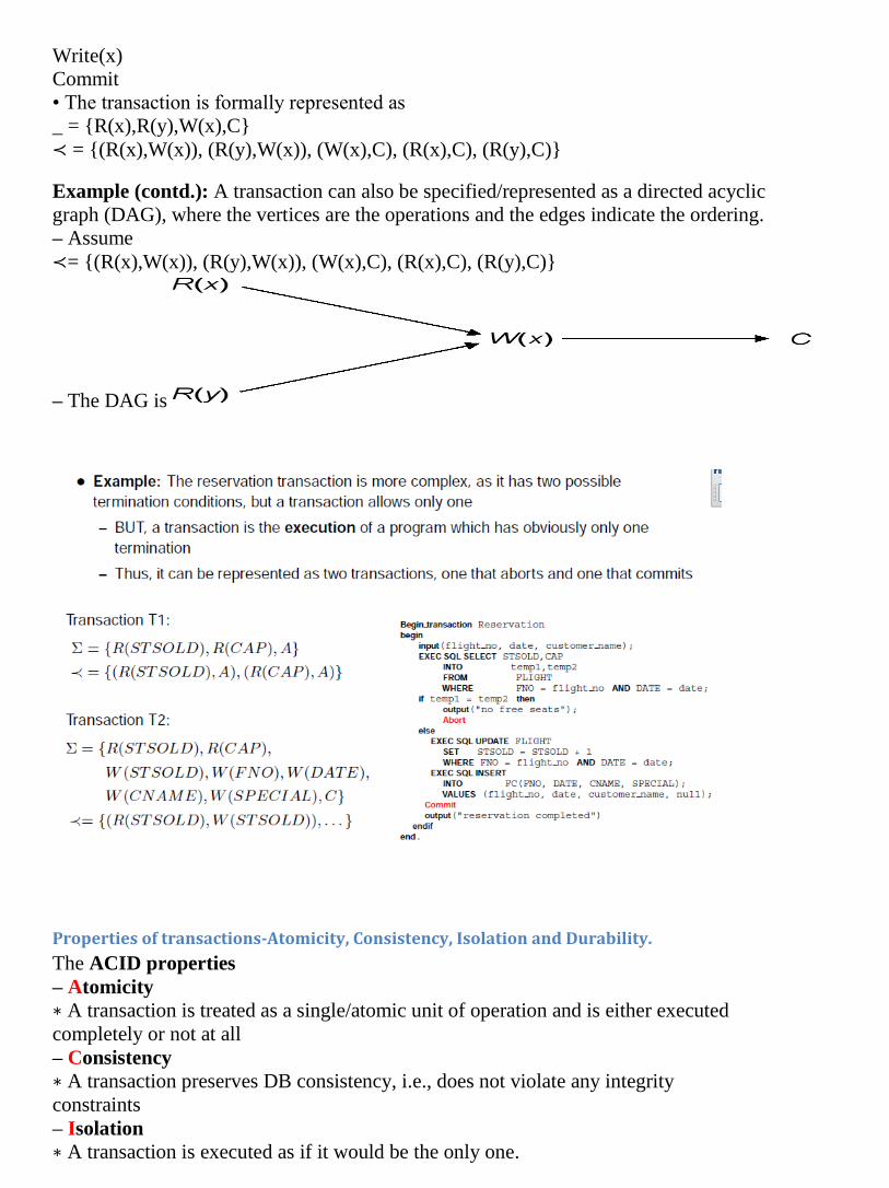
Write(x)
Commit
• The transaction is formally represented as
_ = {R(x),R(y),W(x),C}
≺ = {(R(x),W(x)), (R(y),W(x)), (W(x),C), (R(x),C), (R(y),C)}
Example (contd.): A transaction can also be specified/represented as a directed acyclic
graph (DAG), where the vertices are the operations and the edges indicate the ordering.
– Assume
≺= {(R(x),W(x)), (R(y),W(x)), (W(x),C), (R(x),C), (R(y),C)}
– The DAG is
Properties of transactions-Atomicity, Consistency, Isolation and Durability.
The ACID properties
– Atomicity
∗ A transaction is treated as a single/atomic unit of operation and is either executed
completely or not at all
– Consistency
∗ A transaction preserves DB consistency, i.e., does not violate any integrity
constraints
– Isolation
∗ A transaction is executed as if it would be the only one.

– Durability
∗ The updates of a committed transaction are permanent in the DB
Atomicity
– Either all or none of the transaction’s operations are performed
– Partial results of an interrupted transactions must be undone
– Transaction recovery is the activity of the restoration of atomicity due to input errors,
system overloads, and deadlocks
– Crash recovery is the activity of ensuring atomicity in the presence of system
Crashes
Consistency
– The consistency of a transaction is simply its correctness and ensures that a
transaction transforms a consistent DB into a consistent DB
– Transactions are correct programs and do not violate database integrity constraints
– Dirty data is data that is updated by a transaction that has not yet committed
– Different levels of DB consistency (by Gray et al., 1976)
∗ Degree 0
· Transaction T does not overwrite dirty data of other transactions
∗ Degree 1
· Degree 0 + T does not commit any writes before EOT
∗ Degree 2
· Degree 1 + T does not read dirty data from other transactions
∗ Degree 3
· Degree 2 + Other transactions do not dirty any data read by T before T
Completes
Isolation
– Isolation is the property of transactions which requires each transaction to see a
consistent DB at all times.
– If two concurrent transactions access a data item that is being updated by one of
them (i.e., performs a write operation), it is not possible to guarantee that the second
will read the correct value
– Interconsistency of transactions is obviously achieved if transactions are executed
serially
– Therefore, if several transactions are executed concurrently, the result must be the
same as if they were executed serially in some order (→serializability)

SQL-92 specifies 3 phenomena/situations that occur if proper isolation is not maintained
– Dirty read
∗ T1 modifies x which is then read by T2 before T1 terminates; if T1 aborts, T2 has
read value which never exists in the DB:
– Non-repeatable (fuzzy) read
∗ T1 reads x; T2 then modifies or deletes x and commits; T1 tries to read x again
but reads a different value or can’t find it
– Phantom
∗ T1 searches the database according to a predicate P while T2 inserts new tuples
that satisfy P
****Based on the 3 phenomena, SQL-92 specifies different isolation levels:
– Read uncommitted
∗ For transactions operating at this level, all three phenomena are possible
– Read committed
∗ Fuzzy reads and phantoms are possible, but dirty reads are not
– Repeatable read
∗ Only phantoms possible
– Anomaly serializable
∗ None of the phenomena are possible
• Durability
– Once a transaction commits, the system must guarantee that the results of its
operations will never be lost, in spite of subsequent failures
– Database recovery is used to achieve the task
Classification of Transactions
Classification of transactions according to various criteria
– Duration of transaction
∗ On-line (short-life)
∗ Batch (long-life)
– Organization of read and write instructions in transaction
∗ General model
T1 : {R(x),R(y),W(y),R(z),W(x),W(z),W(w),C}

∗ Two-step (all reads before writes)
T2 : {R(x),R(y),R(z),W(x),W(z),W(y),W(w),C}
∗ Restricted (a data item has to be read before an update)
T3 : {R(x),R(y),W(y),R(z),W(x),W(z),R(w),W(w),C}
∗ Action model: each (read,write) pair is executed atomically
T2 : {[R(x),W(x)], [R(y),W(y)], [R(z),W(z)], [R(w),W(w)],C}
Classification of transactions according to various criteria . . .
– Structure of transaction
∗ Flat transaction
· Consists of a sequence of primitive operations between a begin and end marker
Begin transaction Reservation
...
end.
∗ Nested transaction
· The operations of a transaction may themselves be transactions.
Begin transaction Reservation
...
Begin transaction Airline
...
end.
Begin transaction Hotel
...
end.
end.
∗ Workflows ()
• Workflows: A collection of tasks organized to accomplish a given business process
– Workflows generalize transactions and are more expressive to model complex
business processes
– Types of workflows:
∗ Human-oriented workflows
· Involve humans in performing the tasks.
· System support for collaboration and coordination; but no system-wide
consistency definition
∗ System-oriented workflows
· Computation-intensive and specialized tasks that can be executed by a computer
· System support for concurrency control and recovery, automatic task execution,
notification, etc.
∗ Transactional workflows
· In between the previous two; may involve humans, require access to
heterogeneous, autonomous and/or distributed systems, and support selective
use of ACID properties

Transaction Processing Issues
• Transaction structure (usually called transaction model)
– Flat (simple), nested
• Internal database consistency
– Semantic data control (integrity enforcement) algorithms
• Reliability protocols
– Atomicity and Durability
– Local recovery protocols
– Global commit protocols
• Concurrency control algorithms
– How to synchronize concurrent transaction executions (correctness criterion)
– Intra-transaction consistency, isolation
• Replica control protocols
– How to control the mutual consistency of replicated data
Architectural aspects of Distributed Transaction,
1. Begin transaction. This is an indicator to the TM that a new transaction is starting. The TM does some bookkeeping, such as recording the transaction’s name, the originating application, and so on, in coordination with the data processor. 2. Read. If the data item to be read is stored locally, its value is read and returned to the transaction. Otherwise, the TM finds where the data item is stored and requests its value to be returned (after appropriate concurrency control measures are taken). 3. Write. If the data item is stored locally, its value is updated (in coordination with the data processor). Otherwise, the TM finds where the data item is located and requests the update to be carried out at that site after appropriate concurrency control measures are taken). 4. Commit. The TM coordinates the sites involved in updating data items on behalf of this transaction so that the updates are made permanent at every site. 5. Abort. The TM makes sure that no effects of the transaction are reflected in any of the databases at the sites where it updated data items.

Transaction Serialization.
2.3 Distributed Concurrency Control: Lock-based and Timestamp-based Concurrency
Control methods. Optimistic method for Concurrency Control. Deadlock management-
prevention, avoidance detection, and resolution. Non-serializable schedule and nested
distributed transaction.
Concurrency control is the problem of synchronizing concurrent transactions (i.e.,
order the operations of concurrent transactions) such that the following two properties
are achieved:
– the consistency of the DB is maintained
– the maximum degree of concurrency of operations is achieved
• Obviously, the serial execution of a set of transaction achieves consistency, if each single
transaction is consistent
Conflicting operations: Two operations Oij(x) and Okl(x) of transactions Ti and Tk
are in conflict iff at least one of the operations is a write, i.e.,
– Oij = read(x) and Okl = write(x)
– Oij = write(x) and Okl = read(x)
– Oij = write(x) and Okl = write(x)
• Intuitively, a conflict between two operations indicates that their order of execution is
important.
• Read operations do not conflict with each other, hence the ordering of read operations
does not matter.
• Example: Consider the following two transactions
T1: Read(x) T2: Read(x)
x ← x + 1 x ← x + 1
Write(x) Write(x)
Commit Commit
– To preserve DB consistency, it is important that the read(x) of one transaction is not
between read(x) and write(x) of the other transaction.

Schedules:
Serializability:
• Two schedules are said to be equivalent if they have the same effect on the DB.
• Conflict equivalence: Two schedules S1 and S2 defined over the same set of
transactions T = {T1, T2, . . . , Tn} are said to be conflict equivalent if for each pair
of conflicting operations Oij and Okl, whenever Oij <1 Okl then Oij <2 Okl.
– i.e., conflicting operations must be executed in the same order in both transactions.
• A concurrent schedule is said to be (conflict-)serializable iff it is conflict equivalent to a
serial schedule
• A conflict-serializable schedule can be transformed into a serial schedule by swapping
non-conflicting operations
• Example: Consider the following two schedules
T1: Read(x)
x ← x + 1
Write(x)
Write(z)
Commit
– The schedule {R1(x),W1(x),R2(x),W2(x),W1(z),C2,C1} is
conflict-equivalent to {T1, T2} but not to {T2, T1}
• The primary function of a concurrency controller is to generate a serializable schedule
for the execution of pending transactions.
• In a DDBMS two schedules must be considered
– Local schedule
– Global schedule (i.e., the union of the local schedules)
• Serializability in DDBMS
– Extends in a straightforward manner to a DDBMS if data is not replicated
– Requires more care if data is replicated: It is possible that the local schedules are
serializable, but the mutual consistency of the DB is not guaranteed.
T2: Read(x)
x ← x + 1
Write(x)
Commit
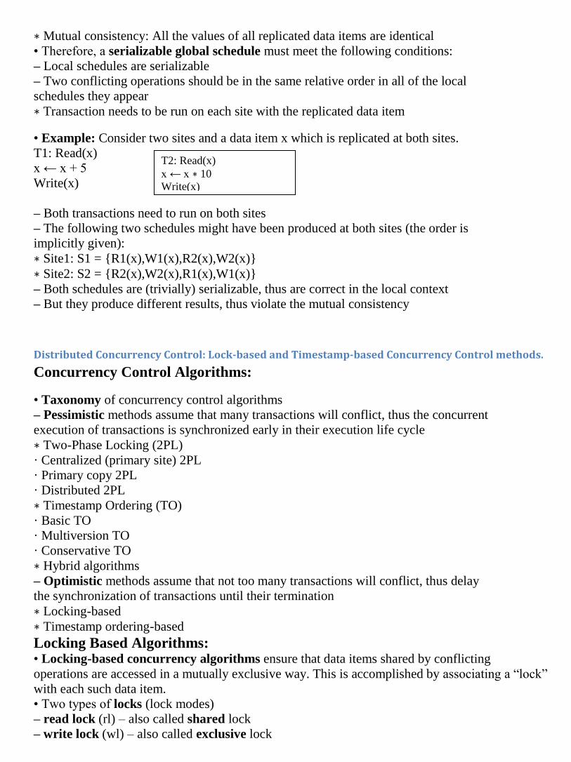
∗ Mutual consistency: All the values of all replicated data items are identical
• Therefore, a serializable global schedule must meet the following conditions:
– Local schedules are serializable
– Two conflicting operations should be in the same relative order in all of the local
schedules they appear
∗ Transaction needs to be run on each site with the replicated data item
• Example: Consider two sites and a data item x which is replicated at both sites.
T1: Read(x)
x ← x + 5
Write(x)
– Both transactions need to run on both sites
– The following two schedules might have been produced at both sites (the order is
implicitly given):
∗ Site1: S1 = {R1(x),W1(x),R2(x),W2(x)}
∗ Site2: S2 = {R2(x),W2(x),R1(x),W1(x)}
– Both schedules are (trivially) serializable, thus are correct in the local context
– But they produce different results, thus violate the mutual consistency
Distributed Concurrency Control: Lock-based and Timestamp-based Concurrency Control methods.
Concurrency Control Algorithms:
• Taxonomy of concurrency control algorithms
– Pessimistic methods assume that many transactions will conflict, thus the concurrent
execution of transactions is synchronized early in their execution life cycle
∗ Two-Phase Locking (2PL)
· Centralized (primary site) 2PL
· Primary copy 2PL
· Distributed 2PL
∗ Timestamp Ordering (TO)
· Basic TO
· Multiversion TO
· Conservative TO
∗ Hybrid algorithms
– Optimistic methods assume that not too many transactions will conflict, thus delay
the synchronization of transactions until their termination
∗ Locking-based
∗ Timestamp ordering-based
Locking Based Algorithms: • Locking-based concurrency algorithms ensure that data items shared by conflicting
operations are accessed in a mutually exclusive way. This is accomplished by associating a “lock”
with each such data item.
• Two types of locks (lock modes)
– read lock (rl) – also called shared lock
– write lock (wl) – also called exclusive lock
T2: Read(x)
x ← x ∗ 10
Write(x)

• Compatibility matrix of locks
• General locking algorithm
1. Before using a data item x, transaction requests lock for x from the lock manager
2. If x is already locked and the existing lock is incompatible with the requested lock, the
transaction is delayed
3. Otherwise, the lock is granted
• Example: Consider the following two transactions
T1: Read(x) T2: Read(x)
x ← x + 1 x ← x ∗ 2
Write(x) Write(x)
Read(y) Read(y)
y ← y – 1 y ← y ∗ 2
Write(y) Write(y)
– The following schedule is a valid locking-based schedule (lri(x) indicates the
release of a lock on x):
S = {wl1(x),R1(x),W1(x), lr1(x)
wl2(x),R2(x),W2(x), lr2(x)
wl2(y),R2(y),W2(y), lr2(y)
wl1(y),R1(y),W1(y), lr1(y)}
– However, S is not serializable
∗ S cannot be transformed into a serial schedule by using only non-conflicting swaps
∗ The result is different from the result of any serial execution
Two-Phase Locking (2PL): • Two-phase locking protocol
– Each transaction is executed in two phases
∗ Growing phase: the transaction obtains locks
∗ Shrinking phase: the transaction releases locks
– The lock point is the moment when transitioning from the growing phase to the
shrinking phase
• Properties of the 2PL protocol
– Generates conflict-serializable schedules
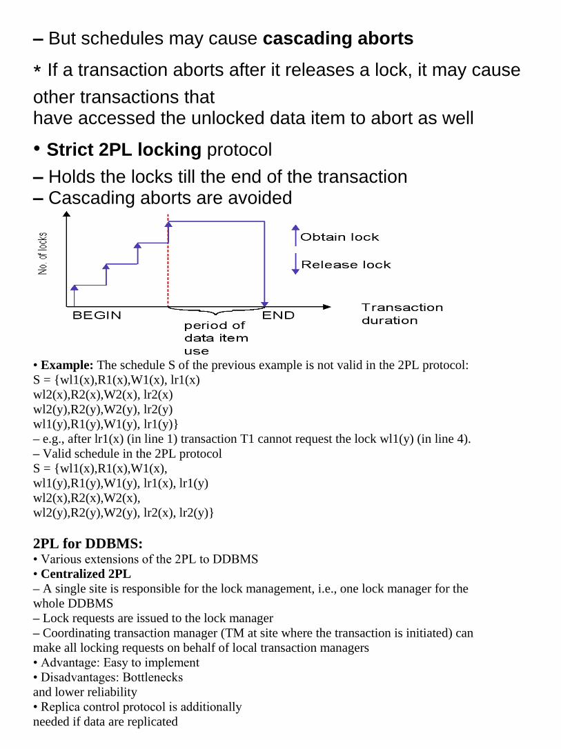
– But schedules may cause cascading aborts
∗ If a transaction aborts after it releases a lock, it may cause
other transactions that have accessed the unlocked data item to abort as well
• Strict 2PL locking protocol
– Holds the locks till the end of the transaction – Cascading aborts are avoided
• Example: The schedule S of the previous example is not valid in the 2PL protocol:
S = {wl1(x),R1(x),W1(x), lr1(x)
wl2(x),R2(x),W2(x), lr2(x)
wl2(y),R2(y),W2(y), lr2(y)
wl1(y),R1(y),W1(y), lr1(y)}
– e.g., after lr1(x) (in line 1) transaction T1 cannot request the lock wl1(y) (in line 4).
– Valid schedule in the 2PL protocol
S = {wl1(x),R1(x),W1(x),
wl1(y),R1(y),W1(y), lr1(x), lr1(y)
wl2(x),R2(x),W2(x),
wl2(y),R2(y),W2(y), lr2(x), lr2(y)}
2PL for DDBMS: • Various extensions of the 2PL to DDBMS
• Centralized 2PL
– A single site is responsible for the lock management, i.e., one lock manager for the
whole DDBMS
– Lock requests are issued to the lock manager
– Coordinating transaction manager (TM at site where the transaction is initiated) can
make all locking requests on behalf of local transaction managers
• Advantage: Easy to implement
• Disadvantages: Bottlenecks
and lower reliability
• Replica control protocol is additionally
needed if data are replicated

(see also primary copy
2PL)
• Primary copy 2PL – Several lock managers are distributed to a number of sites
– Each lock manager is responsible for managing the locks for a set of data items
– For replicated data items, one copy is chosen as primary copy, others are slave
copies
– Only the primary copy of a data item that is updated needs to be write-locked
– Once primary copy has been updated, the change is propagated to the slaves
• Advantages
– Lower communication costs and better performance than the centralized 2PL
• Disadvantages
– Deadlock handling is more complex
• Distributed 2PL – Lock managers are distributed to all sites
– Each lock manager responsible for locks for data at that site
– If data is not replicated, it is equivalent to primary copy 2PL
– If data is replicated, the Read-One-Write-All (ROWA) replica control protocol is
implemented
∗ Read(x): Any copy of a replicated item x can be read by obtaining a read lock on
the copy
∗ Write(x): All copies of x must be write-locked before x can be updated
• Disadvantages
– Deadlock handling more complex
– Communication costs higher than primary copy 2PL
• Communication structure of the distributed 2PL
– The coordinating TM sends the lock request to the lock managers of all participating
sites
– The LMs pass the operations to the data processors
– The end of the operation is signaled to the coordinating TM
Timestamp Ordering: • Timestamp-ordering based algorithms do not maintain serializability by mutual
exclusion, but select (a priori) a serialization order and execute transactions accordingly.
– Transaction Ti is assigned a globally unique timestamp ts(Ti)
– Conflicting operations Oij and Okl are resolved by timestamp order, i.e., Oij is
executed before Okl iff ts(Ti) < ts(Tk).
• To allow for the scheduler to check whether operations arrive in correct order, each data
item is assigned a write timestamp (wts) and a read timestamp (rts):
– rts(x): largest timestamp of any read on x
– wts(x): largest timestamp of any write on x
• Then the scheduler has to perform the following checks:
– Read operation, Ri(x):
∗ If ts(Ti) < wts(x): Ti attempts to read overwritten data; abort Ti
∗ If ts(Ti) ≥ wts(x): the operation is allowed and rts(x) is updated
– Write operations,Wi(x):
∗ If ts(Ti) < rts(x): x was needed before by other transaction; abort Ti
∗ If ts(Ti) < wts(x): Ti writes an obsolete value; abort Ti
∗ Otherwise, executeWi(x)
• Generation of timestamps (TS) in a distributed environment
– TS needs to be locally and globally unique and monotonically increasing
– System clock, incremental event counter at each site, or global counter are unsuitable
(difficult to maintain)
– Concatenate local timestamp/counter with a unique site identifier:
<local timestamp, site identifier>
∗ site identifier is in the least significant position in order to distinguish only if the local
timestamps are identical
• Schedules generated by the basic TO protocol have the following properties:
– Serializable
– Since transactions never wait (but are rejected), the schedules are deadlock-free
– The price to pay for deadlock-free schedules is the potential restart of a transaction
several times
• Basic timestamp ordering is “aggressive”: It tries to execute an operation as soon as it
receives it
• Conservative timestamp ordering delays each operation until there is an assurance that
it will not be restarted, i.e., that no other transaction with a smaller timestamp can arrive
– For this, the operations of each transaction are buffered until an ordering can be
established so that rejections are not possible
• If this condition can be guaranteed, the scheduler will never reject an operation
• However, this delay introduces the possibility for deadlocks
• Multiversion timestamp ordering
– Write operations do not modify the DB; instead, a new version of the data item is
created: x1, x2, . . . , xn
– Ri(x) is always successful and is performed on the appropriate version of x, i.e., the
version of x (say xv) such that wts(xv) is the largest timestamp less than ts(Ti)
– Wi(x) produces a new version xw with ts(xw) = ts(Ti) if the scheduler has not
yet processed any Rj(xr) on a version xr such that
ts(Ti) < rts(xr)
i.e., the write is too late.

– Otherwise, the write is rejected.
• The previous concurrency control algorithms are pessimistic
Optimistic method for Concurrency Control.
• Optimistic concurrency control algorithms
– Delay the validation phase until just before the write phase
– Ti run independently at each site on local copies of the DB (without updating the DB)
– Validation test then checks whether the updates would maintain the DB consistent:
∗ If yes, all updates are performed
∗ If one fails, all Ti’s are rejected
Potentially allow for a higher level of concurrency
Deadlock management- prevention, avoidance detection, and resolution.
• Deadlock: A set of transactions is in a deadlock situation if several transactions wait for
each other. A deadlock requires an outside intervention to take place.
• Any locking-based concurrency control algorithm may result in a deadlock, since there is
mutual exclusive access to data items and transactions may wait for a lock
• Some TO-based algorihtms that require the waiting of transactions may also cause
deadlocks
• A Wait-for Graph (WFG) is a useful tool to identify deadlocks
– The nodes represent transactions
– An edge from Ti to Tj indicates that Ti is waiting for Tj
– If the WFG has a cycle, we have a deadlock situation
• Deadlock management in a DDBMS is more complicate, since lock management is not
centralized
• We might have global deadlock, which involves transactions running at different sites
• A Local Wait-for-Graph (LWFG) may not show the existence of global deadlocks
• A Global Wait-for Graph (GWFG), which is the union of all LWFGs, is needed
• Example: Assume T1 and T2 run at site 1, T3 and T4 run at site 2, and the following
wait-for relationships between them: T1 → T2 → T3 → T4 → T1. This deadlock
cannot be detected by the LWFGs, but by the GWFG which shows intersite waiting.
– Local WFG:

– Global WFG:
Deadlock Prevention: • Deadlock prevention: Guarantee that deadlocks never occur
– Check transaction when it is initiated, and start it only if all required resources are
available.
– All resources which may be needed by a transaction must be predeclared
• Advantages
– No transaction rollback or restart is involved
– Requires no run-time support
• Disadvantages
– Reduced concurrency due to pre-allocation
– Evaluating whether an allocation is safe leads to added overhead
– Difficult to determine in advance the required resources
Deadlock Avoidance: • Deadlock avoidance: Detect potential deadlocks in advance and take actions to ensure
that a deadlock will not occur. Transactions are allowed to proceed unless a requested
resource is unavailable
• Two different approaches:
– Ordering of data items: Order data items and sites; locks can only be requested in
that order (e.g., graph-based protocols)
– Prioritize transactions: Resolve deadlocks by aborting transactions with higher or
lower priority. The following schemes assume that Ti requests a lock hold by Tj :
∗ Wait-Die Scheme: if ts(Ti) < ts(Tj) then Ti waits else Ti dies
∗ Wound-Wait Scheme: if ts(Ti) < ts(Tj) then Tj wounds (aborts) else Ti waits
• Advantages
– More attractive than prevention in a database environment
– Transactions are not required to request resources a priori
• Disadvantages
– Requires run time support
Deadlock Detection • Deadlock detection and resolution: Transactions are allowed to wait freely, and hence
to form deadlocks. Check global wait-for graph for cycles. If a deadlock is found, it is
resolved by aborting one of the involved transactions (also called the victim).
• Advantages
– Allows maximal concurrency
– The most popular and best-studied method
• Disadvantages
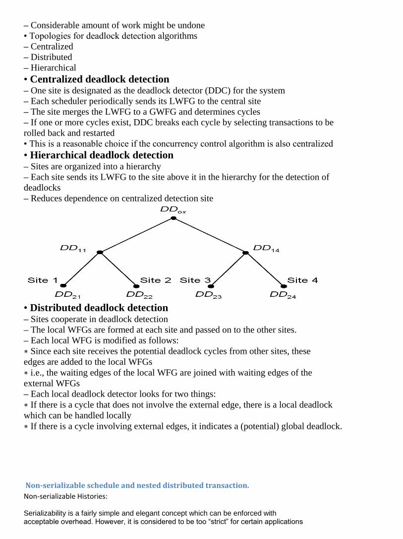
– Considerable amount of work might be undone
• Topologies for deadlock detection algorithms
– Centralized
– Distributed
– Hierarchical • Centralized deadlock detection – One site is designated as the deadlock detector (DDC) for the system
– Each scheduler periodically sends its LWFG to the central site
– The site merges the LWFG to a GWFG and determines cycles
– If one or more cycles exist, DDC breaks each cycle by selecting transactions to be
rolled back and restarted
• This is a reasonable choice if the concurrency control algorithm is also centralized
• Hierarchical deadlock detection – Sites are organized into a hierarchy
– Each site sends its LWFG to the site above it in the hierarchy for the detection of
deadlocks
– Reduces dependence on centralized detection site
• Distributed deadlock detection – Sites cooperate in deadlock detection
– The local WFGs are formed at each site and passed on to the other sites.
– Each local WFG is modified as follows:
∗ Since each site receives the potential deadlock cycles from other sites, these
edges are added to the local WFGs
∗ i.e., the waiting edges of the local WFG are joined with waiting edges of the
external WFGs
– Each local deadlock detector looks for two things:
∗ If there is a cycle that does not involve the external edge, there is a local deadlock
which can be handled locally
∗ If there is a cycle involving external edges, it indicates a (potential) global deadlock.
Non-serializable schedule and nested distributed transaction.
Non-serializable Histories:
Serializability is a fairly simple and elegant concept which can be enforced with acceptable overhead. However, it is considered to be too “strict” for certain applications
since it does not consider as correct certain histories that might be argued as reasonable. We have shown one case when we discussed the ordered shared lock concept. In addition, consider the Reservation transaction of Example 10.10. One can argue that the history generated by two concurrent executions of this transaction can be non-serializable, but correct – one may do the Airline reservation first and then do the Hotel reservation while the other one reverses the order – as long as both executions successfully terminate. The question, however, is how one can generalize these intuitive observations. The solution is to observe and exploit the “semantics” of these transactions. There have been a number of proposals for exploiting transaction semantics. Of particular interest for distributed DBMS is one class that depends on identifying transaction steps, which may consist of a single operation or a set of operations, and establishing how transactions can interleave with each other between steps. Garcia- Molina [1983] classifies transactions into classes such that transactions in the same class are compatible and can interleave arbitrarily while transactions in different classes are incompatible and have to be synchronized. The synchronization is based on semantic notions, allowing more concurrency than serializability. The use of the concept of transaction classes can be traced back to SDD-1 [Bernstein et al., 1980b]. The concept of compatibility is refined by Lynch [1983b] and several levels of compatibility among transactions are defined. These levels are structured hierarchically so that interleavings at higher levels include those at lower levels. Furthermore, Lynch [1983b] introduces the concept of breakpoints within transactions, which represent points at which other transactions can interleave. This is an alternative to the use of compatibility sets. Another work along these lines uses breakpoints to indicate the interleaving points, but does not require that the interleavings be hierarchical [Farrag and O¨ zsu, 1989]. A transaction is modeled as consisting of a number of steps. Each step consists of a sequence of atomic operations and a breakpoint at the end of these operations. For each breakpoint in a transaction the set of transaction types that are allowed to interleave at that breakpoint is specified. A correctness criterion called relative consistency is defined based on the correct interleavings among transactions. Intuitively, a relatively consistent history is equivalent to a history that is stepwise serial (i.e., the operations and breakpoint of each step appear without interleaving), and in which a step (Tik) of transaction Ti interleaves two consecutive steps (Tjm and Tjm+1) of transaction Tj only if transactions of Ti’s type are allowed to interleave Tjm
at its breakpoint. It can be shown that some of the relatively consistent histories are not serializable, but are still “correct” [Farrag and O¨ zsu, 1989]. A unifying framework that combines the approaches of Lynch [1983b] and Farrag and O¨ zsu [1989] has been proposed by Agrawal et al. [1994]. A correctness criterion called semantic relative atomicity is introduced which provides finer interleavings and more concurrency.
Nested Distributed Transactions:
We introduced the nested transaction model in the previous chapter. The concurrent execution of nested transactions is interesting, especially since they are good candidates for distributed execution. Let us first consider closed nested transactions [Moss, 1985]. The concurrency control of nested transactions have generally followed a locking-based approach. The following rules govern the management of the locks and the completion of transaction execution in the case of closed nested transactions: 1. Each subtransaction executes as a transaction and upon completion transfers its lock to its parent transaction. 2. A parent inherits both the locks and the updates of its committed subtransactions. 3. The inherited state will be visible only to descendants of the inheriting parent transaction. However, to access the sate, a descendant must acquire appropriate locks. Lock conflicts are determined as for flat transactions, except that one ignores inherited locks retained by ancestor’s of the requesting subtransaction. 4. If a subtransaction aborts, then all locks and updates that the subtransaction and its descendants are discarded. The parent of an aborted subtransaction need not, but may, choose to abort.

From the perspective of ACID properties, closed nested transactions relax durability since the effects of successfully completed subtransactions can be erased if an ancestor transaction aborts. They also relax the isolation property in a limited way since they share their state with other subtransactions within the same nested transaction. The distributed execution potential of nested transactions is obvious. After all, nested transactions are meant to improve intra-transaction concurrency and one can view each subtransaction as a potential unit of distribution if data are also appropriately distributed. However, from the perspective of lock management, some care has to be observed. When subtransactions release their locks to their parents, these lock releases cannot be reflected in the lock tables automatically. The subtransaction commit commands do not have the same semantics as flat transactions. Open nested transactions are even more relaxed than their closed nested counterparts. They have been called “anarchic” forms of nested transactions [Gray and Reuter, 1993]. The open nested transaction model is best exemplified in the saga model [Garcia-Molina and Salem, 1987; Garcia-Molina et al., 1990] which was discussed in Section 10.3.2. From the perspective of lock management, open nested transactions are easy to deal with. The locks held by a subtransaction are released as soon as it commits or aborts and this is reflected in the lock tables. A variant of open nested transactions with precise and formal semantics is the multilevel transaction model [Weikum, 1986; Weikum and Schek, 1984; Beeri et al., 1988; Weikum, 1991]. Multilevel transactions “are a variant of open nested transactions in which the subtransactions correspond to operations at different levels of a layered system architecture” [Weikum and Hasse, 1993]. We introduce the concept with an example taken from [Weikum, 1991]. We consider a transaction specification language which allows users to write transactions involving abstract operations so as to be able to exploit application semantics. Consider two transactions that transfer funds from one bank account to another: T1: Withdraw(o; x) T2: Withdraw(o; y) Deposit(p; x) Deposit(p;y) The notation here is that each Ti withdraws x (y) amount from account o and deposits that amount to account p. The semantics of Withdraw is test-and-withdraw to ensure that the account balance is sufficient to meet the withdrawal request. In relational systems, each of these abstract operations will be translated to tuple operations Select (Sel), and Update (Upd) which will, in turn, be translated into page-level Read and Write operations (assuming o is on page r and p is on page w). This results in a layered abstraction of transaction execution as depicted in Figure 11.19.
Fig. 11.19 Multilevel Transaction Example (Based on [Weikum, 1991])
The traditional method of dealing with these types of histories is to develop a scheduler that enforces serializability at the lowest level (L0). This, however, reduces the level of concurrency since it does not take into account application semantics and the granularity of synchronization is too coarse. Abstracting from the lower-level details can provide higher concurrency. For example, the page-level history (L0) in Figure 11.19 is not serializable with respect to transactions T1 and T2, but the tuplelevel
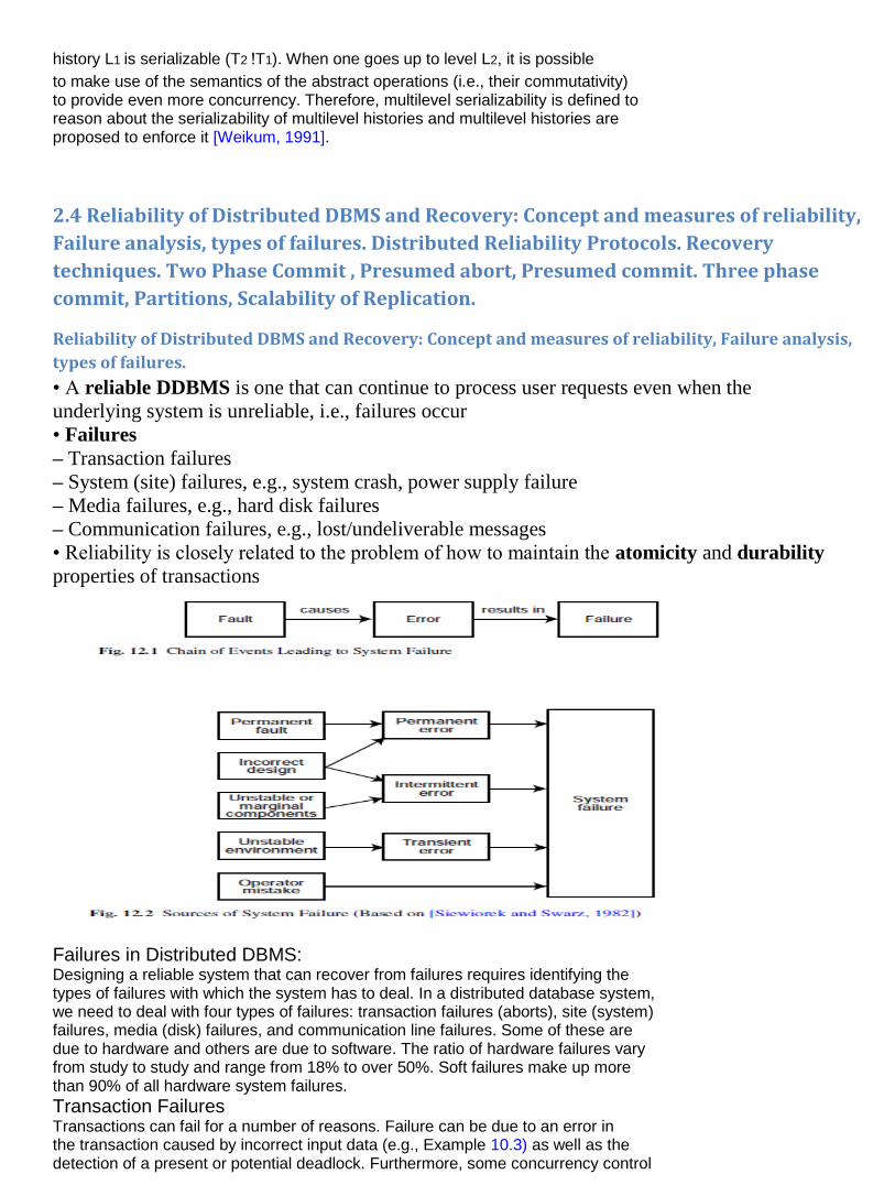
history L1 is serializable (T2 !T1). When one goes up to level L2, it is possible
to make use of the semantics of the abstract operations (i.e., their commutativity) to provide even more concurrency. Therefore, multilevel serializability is defined to reason about the serializability of multilevel histories and multilevel histories are proposed to enforce it [Weikum, 1991].
2.4 Reliability of Distributed DBMS and Recovery: Concept and measures of reliability,
Failure analysis, types of failures. Distributed Reliability Protocols. Recovery
techniques. Two Phase Commit , Presumed abort, Presumed commit. Three phase
commit, Partitions, Scalability of Replication.
Reliability of Distributed DBMS and Recovery: Concept and measures of reliability, Failure analysis,
types of failures.
• A reliable DDBMS is one that can continue to process user requests even when the
underlying system is unreliable, i.e., failures occur
• Failures
– Transaction failures
– System (site) failures, e.g., system crash, power supply failure
– Media failures, e.g., hard disk failures
– Communication failures, e.g., lost/undeliverable messages
• Reliability is closely related to the problem of how to maintain the atomicity and durability
properties of transactions
Failures in Distributed DBMS: Designing a reliable system that can recover from failures requires identifying the types of failures with which the system has to deal. In a distributed database system, we need to deal with four types of failures: transaction failures (aborts), site (system) failures, media (disk) failures, and communication line failures. Some of these are due to hardware and others are due to software. The ratio of hardware failures vary from study to study and range from 18% to over 50%. Soft failures make up more than 90% of all hardware system failures.
Transaction Failures Transactions can fail for a number of reasons. Failure can be due to an error in the transaction caused by incorrect input data (e.g., Example 10.3) as well as the detection of a present or potential deadlock. Furthermore, some concurrency control

algorithms do not permit a transaction to proceed or even to wait if the data that they attempt to access are currently being accessed by another transaction. This might also be considered a failure. The usual approach to take in cases of transaction failure is to abort the transaction, thus resetting the database to its state prior to the start of this transaction.2
The frequency of transaction failures is not easy to measure. An early study reported that in System R, 3% of the transactions aborted abnormally [Gray et al., 1981]. In general, it can be stated that (1) within a single application, the ratio of transactions that abort themselves is rather constant, being a function of the incorrect data, the available semantic data control features, and so on; and (2) the number of transaction aborts by the DBMS due to concurrency control considerations (mainly deadlocks) is dependent on the level of concurrency (i.e., number of concurrent transactions), the interference of the concurrent applications, the granularity of locks, and so on [H¨arder and Reuter, 1983].
Site (System) Failures The reasons for system failure can be traced back to a hardware or to a software failure. The important point from the perspective of this discussion is that a system failure is always assumed to result in the loss of main memory contents. Therefore, any part of the database that was in main memory buffers is lost as a result of a system failure. However, the database that is stored in secondary storage is assumed to be safe and correct. In distributed database terminology, system failures are typically referred to as site failures, since they result in the failed site being unreachable from other sites in the distributed system. We typically differentiate between partial and total failures in a distributed system. Total failure refers to the simultaneous failure of all sites in the distributed system; partial failure indicates the failure of only some sites while the others remain operational. As indicated in Chapter 1, it is this aspect of distributed systems that makes them more available.
Media Failures Media failure refers to the failures of the secondary storage devices that store the database. Such failures may be due to operating system errors, as well as to hardware faults such as head crashes or controller failures. The important point from the perspective of DBMS reliability is that all or part of the database that is on the secondary storage is considered to be destroyed and inaccessible. Duplexing of disk storage and maintaining archival copies of the database are common techniques that deal with this sort of catastrophic problem. Media failures are frequently treated as problems local to one site and therefore not specifically addressed in the reliability mechanisms of distributed DBMSs. We consider techniques for dealing with them in Section 12.3.5 under local recovery management. We then turn our attention to site failures when we consider distributed recovery functions.
Communication Failures The three types of failures described above are common to both centralized and distributed DBMSs. Communication failures, however, are unique to the distributed case. There are a number of types of communication failures. The most common ones are the errors in the messages, improperly ordered messages, lost (or undeliverable) messages, and communication line failures. As discussed in Chapter 2, the first two errors are the responsibility of the computer network; we will not consider them further. Therefore, in our discussions of distributed DBMS reliability, we expect the underlying computer network hardware and software to ensure that two messages sent from a process at some originating site to another process at some destination site are delivered without error and in the order in which they were sent. Lost or undeliverable messages are typically the consequence of communication line failures or (destination) site failures. If a communication line fails, in addition to losing the message(s) in transit, it may also divide the network into two or more disjoint groups. This is called network partitioning. If the network is partitioned, the sites in each partition may continue to operate. In this case, executing transactions that access data stored in multiple partitions becomes a major issue. Network partitions point to a unique aspect of failures in distributed computer systems. In centralized systems the system state can be characterized as all-ornothing:

either the system is operational or it is not. Thus the failures are complete: when one occurs, the entire system becomes non-operational. Obviously, this is not true in distributed systems. As we indicated a number of times before, this is their potential strength. However, it also makes the transaction management algorithms more difficult to design. If messages cannot be delivered, we will assume that the network does nothing about it. It will not buffer it for delivery to the destination when the service is reestablished and will not inform the sender process that the message cannot be delivered. In short, the message will simply be lost.We make this assumption because it represents the least expectation from the network and places the responsibility of dealing with these failures to the distributed DBMS. As a consequence, the distributed DBMS is responsible for detecting that a message is undeliverable is left to the application program (in this case the distributed DBMS). The detection will be facilitated by the use of timers and a timeout mechanism that keeps track of how long it has been since the sender site has not received a confirmation from the destination site about the receipt of a message. This timeout interval needs to be set to a value greater than that of the maximum round-trip propagation delay of a message in the network. The term for the failure of the communication network to deliver messages and the confirmations within this period is performance failure. It needs to be handled within the reliability protocols for distributed DBMSs.
Distributed Reliability Protocols.
• Recovery system: Ensures atomicity and durability of transactions in the presence of
failures (and concurrent transactions)
• Recovery algorithms have two parts
1. Actions taken during normal transaction processing to ensure enough information
exists to recover from failures
2. Actions taken after a failure to recover the DB contents to a state that ensures atomicity,
consistency and durability
Local Recovery Management: • The local recovery manager (LRM) maintains the atomicity and durability properties of
local transactions at each site.
• Architecture
– Volatile storage: The main memory of the computer system (RAM)
– Stable storage
_ A storage that “never” looses its contents
_ In reality this can only be approximated by a combination of hardware (non-volatile
storage) and software (stable-write, stable-read, clean-up) components
• Two ways for the LRM to deal with update/write operations
* In-place update
_ Physically changes the value of the data item in the stable database
_ As a result, previous values are lost

_ Mostly used in databases
* Out-of-place update
_ The new value(s) of updated data item(s) are stored separately from the old
value(s)
_ Periodically, the updated values have to be integrated into the stable DB
In-Place Update: • Since in-place updates cause previous values of the affected data items to be lost, it is
necessary to keep enough information about the DB updates in order to allow recovery
in the case of failures
• Thus, every action of a transaction must not only perform the action, but must also write
a log record to an append-only log file
• A log is the most popular structure for recording DB modifications on stable storage
• Consists of a sequence of log records that record all the update activities in the DB
• Each log record describes a significant event during transaction processing
• Types of log records
– < Ti, start >: if transaction Ti has started
– < Ti,Xj , V1, V2 >: before Ti executes a write(Xj), where V1 is the old value
before the write and V2 is the new value after the write
– < Ti, commit >: if Ti has committed
– < Ti, abort >: if Ti has aborted
– < checkpoint >
• With the information in the log file the recovery manager can restore the consistency of
the DB in case of a failure.
• Assume the following situation when a system crash occurs
• Upon recovery:
– All effects of transaction T1 should be reflected in the database (REDO)
– None of the effects of transaction T2 should be reflected in the database (UNDO)
• REDO Protocol
– REDO’ing an action means performing it again
– The REDO operation uses the log information and performs the action that might
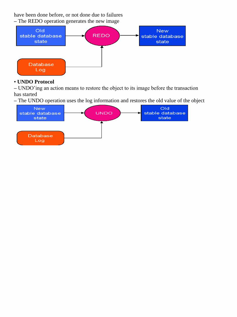
have been done before, or not done due to failures
– The REDO operation generates the new image
• UNDO Protocol
– UNDO’ing an action means to restore the object to its image before the transaction
has started
– The UNDO operation uses the log information and restores the old value of the object
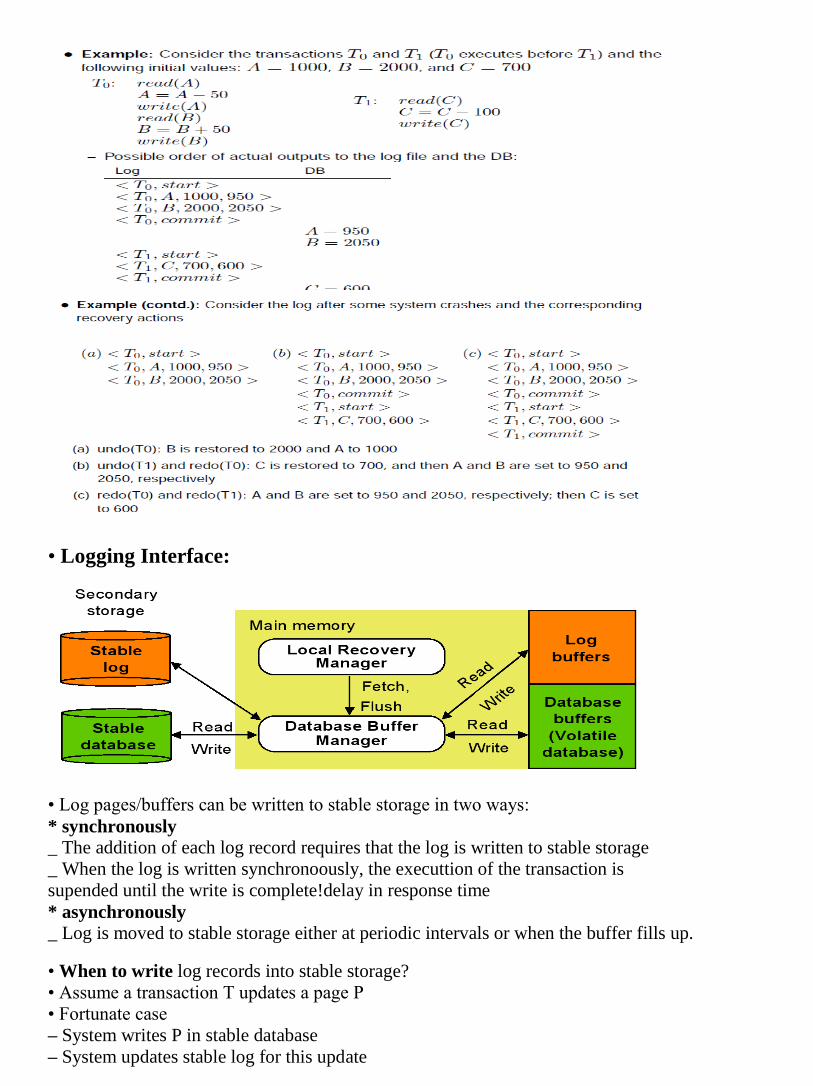
• Logging Interface:
• Log pages/buffers can be written to stable storage in two ways:
* synchronously
_ The addition of each log record requires that the log is written to stable storage
_ When the log is written synchronoously, the executtion of the transaction is
supended until the write is complete!delay in response time
* asynchronously
_ Log is moved to stable storage either at periodic intervals or when the buffer fills up.
• When to write log records into stable storage?
• Assume a transaction T updates a page P
• Fortunate case
– System writes P in stable database
– System updates stable log for this update
– SYSTEM FAILURE OCCURS!... (before T commits)
– We can recover (undo) by restoring P to its old state by using the log
• Unfortunate case
– System writes P in stable database
– SYSTEM FAILURE OCCURS!... (before stable log is updated)
– We cannot recover from this failure because there is no log record to restore the old
value
• Solution: Write-Ahead Log (WAL) protocol
• Notice:
– If a system crashes before a transaction is committed, then all the operations must be
undone. We need only the before images (undo portion of the log)
– Once a transaction is committed, some of its actions might have to be redone. We
need the after images (redo portion of the log)
• Write-Ahead-Log (WAL) Protocol
– Before a stable database is updated, the undo portion of the log should be written to
the stable log
– When a transaction commits, the redo portion of the log must be written to stable log
prior to the updating of the stable database
Out-of-Place Update:
• Two out-of-place strategies are shadowing and differential files
• Shadowing
– When an update occurs, don’t change the old page, but create a shadow page with
the new values and write it into the stable database
– Update the access paths so that subsequent accesses are to the new shadow page
– The old page is retained for recovery
• Differential files
– For each DB file F maintain
_ a read-only part FR
_ a differential file consisting of insertions part (DF+) and deletions part (DF−)
– Thus, F = (FR [ DF+) − DF−
Distributed Reliability Protocols:
• As with local reliability protocols, the distributed versions aim to maintain the atomicity
and durability of distributed transactions
• Most problematic issues in a distributed transaction are commit, termination, and
recovery
* Commit protocols
_ How to execute a commit command for distributed transactions
_ How to ensure atomicity (and durability)?
*Termination protocols
_ If a failure occurs at a site, how can the other operational sites deal with it
_ Non-blocking: the occurrence of failures should not force the sites to wait until the
failure is repaired to terminate the transaction
*Recovery protocols
_ When a failure occurs, how do the sites where the failure occurred deal with it

_ Independent: a failed site can determine the outcome of a transaction without
having to obtain remote information
Commit Protocols:
• Primary requirement of commit protocols is that they maintain the atomicity of distributed
transactions (atomic commitment)
– i.e., even though the exectution of the distributed transaction involves multiple sites,
some of which might fail while executing, the effects of the transaction on the
distributed DB is all-or-nothing.
• In the following we distinguish two roles
– Coordinator: The process at the site where the transaction originates and which
controls the execution
– Participant: The process at the other sites that participate in executing the transaction
Centralized Two Phase Commit Protocol (2PC):
• Very simple protocol that ensures the atomic commitment of distributed transactions.
• Phase 1: The coordinator gets the participants ready to write the results into the
database
• Phase 2: Everybody writes the results into the database
• Global Commit Rule
– The coordinator aborts a transaction if and only if at least one participant votes to
abort it
– The coordinator commits a transaction if and only if all of the participants vote to
commit it
• Centralized since communication is only between coordinator and the participants

Linear 2PC Protocol
• There is linear ordering between the sites for the purpose of communication
• Minimizes the communication, but low response time as it does not allow any parallelism
Distributed 2PC Protocol
• Distributed 2PC protocol increases the communication between the nodes
• Phase 2 is not needed, since each participant sends its vote to all other participants (+
the coordinator), thus each participants can derive the global decision

2PC Protocol and Site Failures
• Site failures in the 2PC protocol might lead to timeouts
• Timeouts are served by termination protocols
• We use the state transition diagrams of the 2PC for the analysis
• Coordinator timeouts: One of the participants is down. Depending on the state, the
coordinator can take the following actions:
*Timeout in INITIAL
_ Do nothing
*Timeout in WAIT
_ Coordinator is waiting for local decisions
_ Cannot unilaterally commit
_ Can unilaterally abort and send an appropriate message to all participants
*Timeout in ABORT or COMMIT
_ Stay blocked and wait for the acks (indefinitely if the site is down indefinitely)
• Participant timeouts: The coordinator site is down. A participant site is in
– Timeout in INITIAL
_ Participant waits for “prepare”, thus coordinator must have failed in INITIAL state

_ Participant can unilaterally abort
– Timeout in READY
_ Participant has voted to commit, but does not know the global decision
_ Participant stays blocked (indefinitely, if the coordinator is permanently down),
since participant cannot change its vote or unilaterally decide to commit
• The actions to be taken after a recovery from a failure are specified in the recovery
protocol
• Coordinator site failure: Upon recovery, it takes the following actions:
*Failure in INITIAL
_ Start the commit process upon recovery (since coordinator did not send anything
to the sites)
*Failure in WAIT
_ Restart the commit process upon recovery (by sending “prepare” again to the
participants)
*Failure in ABORT or COMMIT
_ Nothing special if all the acks have been received from participants
_ Otherwise the termination protocol is involved (re-ask the acks)

• Additional cases
– Coordinator site fails after writing ”begin commit” log and before sending ”prepare”
command
_ treat it as a failure in WAIT state; send ”prepare” command
– Participant site fails after writing ”ready” record in log but before ”vote-commit” is sent
_ treat it as failure in READY state
_ alternatively, can send ”vote-commit” upon recovery
– Participant site fails after writing ”abort” record in log but before ”vote-abort” is sent
_ no need to do anything upon recovery
– Coordinator site fails after logging its final decision record but before sending its
decision to the participants
_ coordinator treats it as a failure in COMMIT or ABORT state
_ participants treat it as timeout in the READY state
– Participant site fails after writing ”abort” or ”commit” record in log but before
acknowledgement is sent
_ participant treats it as failure in COMMIT or ABORT state
_ coordinator will handle it by timeout in COMMIT or ABORT state
Problems with 2PC Protocol:
• A protocol is non-blocking if it permits a transaction to terminate at the operational sites
without waiting for recovery of the failed site.
– Significantly improves the response-time of transactions
• 2PC protocol is blocking
– Ready implies that the participant waits for the coordinator
– If coordinator fails, site is blocked until recovery; independent recovery is not possible
– The problem is that sites might be in both: commit and abort phases.
Three Phase Commit Protocol (3PC):
• 3PC is a non-blocking protocol when failures are restricted to single site failures
• The state transition diagram contains
– no state which is ”adjacent” to both a commit and an abort state
– no non-committable state which is ”adjacent” to a commit state
• Adjacent: possible to go from one status to another with a single state transition
• Committable: all sites have voted to commit a transaction (e.g.: COMMIT state)
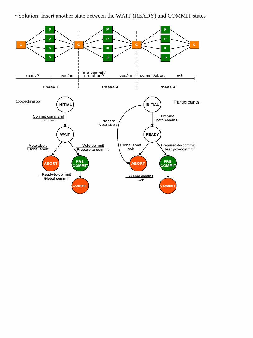
• Solution: Insert another state between the WAIT (READY) and COMMIT states
Recovery techniques.
Two Phase Commit , Presumed abort, Presumed commit.
Three phase commit, Partitions, Scalability of Replication.
Unit 3: 16 hrs.
3.1 Object Oriented Database Concept: Data types and Object, Evolution of Object
Oriented Concepts, Characteristics of Object Oriented Data Model. Object Hierarchies -
Generalization, Specialization, Aggregation. Object Schema. Inter-object Relationships,
Similarities and difference between Object Oriented Database model and Other Data
models.
Object Oriented Database Concept: Data types and Object, Evolution of Object Oriented Concepts,
The term object-oriented—abbreviated by OO or O-O—has its origins in OO programming languages, or OOPLs. Today OO
concepts are applied in the areas of databases, software engineering, knowledge bases, artificial intelligence, and computer
systems in general. OOPLs have their roots in the SIMULA language, which was proposed in the late 1960s. In SIMULA, the
concept of a class groups together the internal data structure of an object in a class declaration. Subsequently, researchers
proposed the concept of abstract data type, which hides the internal data structures and specifies all possible external
operations that can be applied to an object, leading to the concept of encapsulation. The programming language
SMALLTALK, developed at Xerox PARC (Note 9) in the 1970s, was one of the first languages to explicitly incorporate
additional OO concepts, such as message passing and inheritance. It is known as a pure OO programming language, meaning
that it was explicitly designed to be object-oriented. This contrasts with hybrid OO programming languages, which
incorporate OO concepts into an already existing language. An example of the latter is C++, which incorporates OO concepts
into the popular C programming language.
An object typically has two components: state (value) and behavior (operations). Hence, it is somewhat similar to a program
variable in a programming language, except that it will typically have a complex data structure as well as specific operations
defined by the programmer (Note 10). Objects in an OOPL exist only during program execution and are hence called
transient objects. An OO database can extend the existence of objects so that they are stored permanently, and hence the
objects persist beyond program termination and can be retrieved later and shared by other programs. In other words, OO
databases store persistent objects permanently on secondary storage, and allow the sharing of these objects among multiple
programs and applications. This requires the incorporation of other well-known features of database management systems,
such as indexing mechanisms, concurrency control, and recovery. An OO database system interfaces with one or more OO
programming languages to provide persistent and shared object capabilities.
Another key concept in OO systems is that of type and class hierarchies and inheritance. This permits specification of new
types or classes that inherit much of their structure and operations from previously defined types or classes. Hence,
specification of object types can proceed systematically. This makes it easier to develop the data types of a system
incrementally, and to reuse existing type definitions when creating new types of objects.
Evolution:
Traditional data models and systems, such as relational, network, and hierarchical, have been quite successful in developing
the database technology required for many traditional business database applications. However, they have certain
shortcomings when more complex database applications must be designed and implemented—for example, databases for
engineering design and manufacturing (CAD/CAM and CIM (Note 2)), scientific experiments, telecommunications, geographic
information systems, and multimedia (Note 3). These newer applications have requirements and characteristics that differ
from those of traditional business applications, such as more complex structures for objects, longer-duration transactions,
new data types for storing images or large textual items, and the need to define nonstandard application-specific operations.
Object-oriented databases were proposed to meet the needs of these more complex applications. The object-oriented
approach offers the flexibility to handle some of these requirements without being limited by the data types and query
languages available in traditional database systems. A key feature of object-oriented databases is the power they give the
designer to specify both the structure of complex objects and the operations that can be applied to these objects.
Another reason for the creation of object-oriented databases is the increasing use of object-oriented programming
languages in developing software applications. Databases are now becoming fundamental components in many software
systems, and traditional databases are difficult to use when embedded in object-oriented software applications that are
developed in an object-oriented
programming language such as C++, SMALLTALK, or JAVA. Object-oriented databases are designed so they can be directly—
or seamlessly—integrated with software that is developed using object-oriented programming languages.
The need for additional data modeling features has also been recognized by relational DBMS vendors, and the newer
versions of relational systems are incorporating many of the features that were proposed for object-oriented databases. This
has led to systems that are characterized as object-relational or extended relational DBMSs (see Chapter 13). The next
version of the SQL standard for relational DBMSs, SQL3, will include some of these features.
In the past few years, many experimental prototypes and commercial object-oriented database systems have been created.
The experimental prototypes include the ORION system developed at MCC (Note 4), OPENOODB at Texas Instruments, the
IRIS system at Hewlett-Packard laboratories, the ODE system at AT&T Bell Labs (Note 5), and the ENCORE/ObServer project
at Brown University. Commercially available systems include GEMSTONE/OPAL of GemStone Systems, ONTOS of Ontos,
Objectivity of Objectivity Inc., Versant of Versant Object Technology, ObjectStore of Object Design, ARDENT of ARDENT
Software (Note 6), and POET of POET Software. These represent only a partial list of the experimental prototypes and the
commercially available object-oriented database systems.
As commercial object-oriented DBMSs became available, the need for a standard model and language was recognized.
Because the formal procedure for approval of standards normally takes a number of years, a consortium of object-oriented
DBMS vendors and users, called ODMG (Note 7), proposed a standard that is known as the ODMG-93 standard, which has
since been revised with the latest version being ODMG version 2.0.
Object-oriented databases have adopted many of the concepts that were developed originally for object-oriented
programming languages. It contains origins of the object-oriented approach and how it applies to database systems, key
concepts utilized in many object-oriented database systems. discusses object identity, object structure, and type
constructors, encapsulation of operations and definition of methods as part of class declarations, and also discusses the
mechanisms for storing objects in a database by making them persistent, type and class hierarchies and inheritance in
object-oriented databases ,issues that arise when complex objects need to be represented and stored, polymorphism,
operator overloading, dynamic binding, multiple and selective inheritance, and versioning and configuration of objects.
Characteristics of Object Oriented Data Model.
• Creating Abstract Data types
• Embedding the object types to tables
• Using Constructor methods
• Use of Varrays
• Use of Nested Tables
• Using REF and DEREF constructs
• Using Member Functions
• Using object views
b) Embedding the object types to tables:
• Objects that appear in object tables are called row objects.
• Objects that appear only in table columns or as attributes of other objects are called column objects.
• An embedded object is one that is completely contained within another.
• A column object is one that is represented as a column in a table.
• To take advantage of OO capabilities, a database must also support ROW OBJECTS – Objects that are represented as
rows instead of columns.
• Object tables are used to establish a master-child relationship between objects.
Object Tables And OID (ROW OBJECTS)
• An object table is a special kind of table that holds objects and provides a relational view of the attributes of those
objects. In an object table, each row is a row object.
• Example
CREATE OR REPLACE TYPE deptype AS OBJECT
(
deptno NUMBER,
dname VARCHAR2(20),
loc VARCHAR2(20)
);
Embedding the object types to tables:
Object Tables
Example
CREATE OR REPLACE TYPE deptype AS OBJECT
(
deptno NUMBER,
dname VARCHAR2(20),
loc VARCHAR2(20)
);
• This is a simple object type. To create a table out of this object type, the following syntax must be used.
CREATE TABLE deptab OF deptype;
REFs
• In the relational model, foreign keys express many—to—one relationship.
• Object option provides a more efficient means of expressing many-to-one relationships when the “one” side of the
relationship is a row object.
• REFs only describe a relationship in one direction.
• Consider the deptab object table created using the deptype abstract data type :
CREATE TABLE EMPLOYEES
(
EMPNO NUMBER,
ename VARCHAR2(20),
deptno REF deptype );
• In the above example, DEPTNO column references data that is stored elsewhere. The REF operator points the
DEPTNO column to the DEPTYPE data type.
Using Object Views
With object views, you can achieve the following benefits:
• Efficiency of object access: In PL/SQL, and particularly in Oracle Call Interface (OCI) applications, object programming
constructs provide for convenient retrieval, caching, and updating of object data.
• Ability to navigate using REFs.: Can retrieve attributes from related "virtual objects" using dot notation rather than
explicit joins.
• Easier schema evolution: object views offer more ways that you can change both table structure and object type
definitions of an existing system.
• Consistency with new object-based applications: The new components can be implemented in object tables; new
object-oriented applications requiring access to existing data can employ a consistent programming model.
Member Functions
• When dealing with numbers, common convention dictates that the number with the larger value is greater than the
other.
• But when objects are compared, the attributes based on the comparison may not be determined.
• In order to compare objects, Oracle allows declaring two
types of member functions called MAP and ORDER.
MAP
• Map Function is used to specify a single numeric value that is used to compare two objects of the same type.
• The greater than or less than or equality is based on this value.
ORDER
• Order Function is used to write the specific code in order to compare two objects and the return value indicates the
equality or greater or lesser comparisons.
Object Hierarchies - Generalization, Specialization, Aggregation. Object Schema.
Class Definition Example
class employee {
/* Variables */
String name;
string address;
Date start-date;
int salary ;
/* Messages */
int annual-salary ();
string get-name();
string get-address();
int set-address(string new-address);
int employment-length();
};
Object Hierarchies(generalisation-specialization)
• E.g., class of bank customers similar to class of bank employees: both share some variables and messages, e.g.,
name and address.
• But there are variables and messages specific to each class e.g., salary for employees and credit-rating for
customers.
• Every employee is a person; thus employee is a specialization of person
• Similarly, customer is a specialization of person.
• Create classes person, employee and customer
• – variables/messages applicable to all persons associated with class person.
• – variables/messages specific to employees associated with class employee; similarly for customer

class person {
string name;
string address; } ;
class customer isa person {
int credit-rating; };
class employee isa person {
date start-date;
int salary ; };
class officer isa employee {
int office-number ;
int expense-account-number ;};
• Full variable list for objects in the class officer:
• office-number, expense-account-number: defined locally
• start-date, salary: inherited from employee
• name, address: inherited from person
• Methods are inherited similar to variables.
• Generalization/Specialization is the IS A relationship, which is supported in OODB through class hierarchy.
• E.g. An ArtBook is a Book, therefore the ArtBook class is a subclass of Book class. A subclass inherits all the attribute
and method of its super class.
• Three subclasses—Officer, Clerks and Secretary are generalized into a super class called Employee.
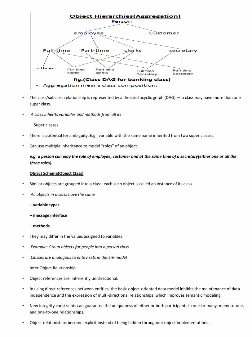
• The class/subclass relationship is represented by a directed acyclic graph (DAG) — a class may have more than one
super class.
• A class inherits variables and methods from all its
Super classes.
• There is potential for ambiguity. E.g., variable with the same name inherited from two super classes.
• Can use multiple inheritance to model “roles” of an object.
e.g. a person can play the role of employee, customer and at the same time of a secretary(either one or all the
three roles).
Object Schema(Object Class)
• Similar objects are grouped into a class; each such object is called an instance of its class.
• All objects in a class have the same
– variable types
– message interface
– methods
• They may differ in the values assigned to variables
• Example: Group objects for people into a person class
• Classes are analogous to entity sets in the E-R model
Inter Object Relationship
• Object references are inherently unidirectional.
• In using direct references between entities, the basic object-oriented data model inhibits the maintenance of data
independence and the expression of multi-directional relationships, which improves semantic modeling.
• New integrity constraints can guarantee the uniqueness of either or both participants in one-to-many, many-to-one,
and one-to-one relationships.
• Object relationships become explicit instead of being hidden throughout object implementations .

• The use of relationships enhances the data independence of a database.
• An inter-object relationship indicates that the referenced object should be the most current, and transient version.
• An inter-object relationship indicates that the referenced object should be a specific working version.
Differences in Data Models
• The type of a database is decided by the data model used in the design of the database.
• Data models are data structures which describe how data are represented and accessed.
Hierarchical model contains data organized into a tree-like structure.
This supports parent-child relationships between data similar to a tree data structure where object types are
represented by nodes and their relationships are represented by arcs.
• This model is restrictive in that it only allows one to many relationship ( a parent can have many children but a child
can only have one parent)
• Network Model is similar to the hierarchical model in representation of data but allows for greater flexibility in data
access as it supports many to many relationships.
• Relational Model organizes data into two dimensional arrays known as relations(tables) and each relation consists of
rows and columns.
• Another major characteristic of relational model is that of keys – designated columns in a relation used to order data
or establish relations.
• Object Data Model aims to reduce the overhead of converting information representation in the database to an
application specific representation.
• object model allows for data persistence and storage by storing objects in the databases .
• The relationships between various objects are inherent in the structure of the objects.
• This is mainly used for complex data structures.
• Object oriented databases or object databases incorporate the object data model to define data structures on
which database operations such as CRUD can be performed.
• They store objects rather than data such as integers and strings. The relationship between various data is implicit to
the object and manifests as object attributes and methods
• Object database management systems extend the object programming language with transparently persistent data,
concurrency control, data recovery, associative queries, and other database capabilities.
Similarities
• An object corresponds to an entity in the E-R model.
• The object-oriented paradigm is based on encapsulating code and data related to an object into a single unit.
• The object-oriented data model is a logical model like the E-R model.
• Comparison between OODBMS and RDBMS
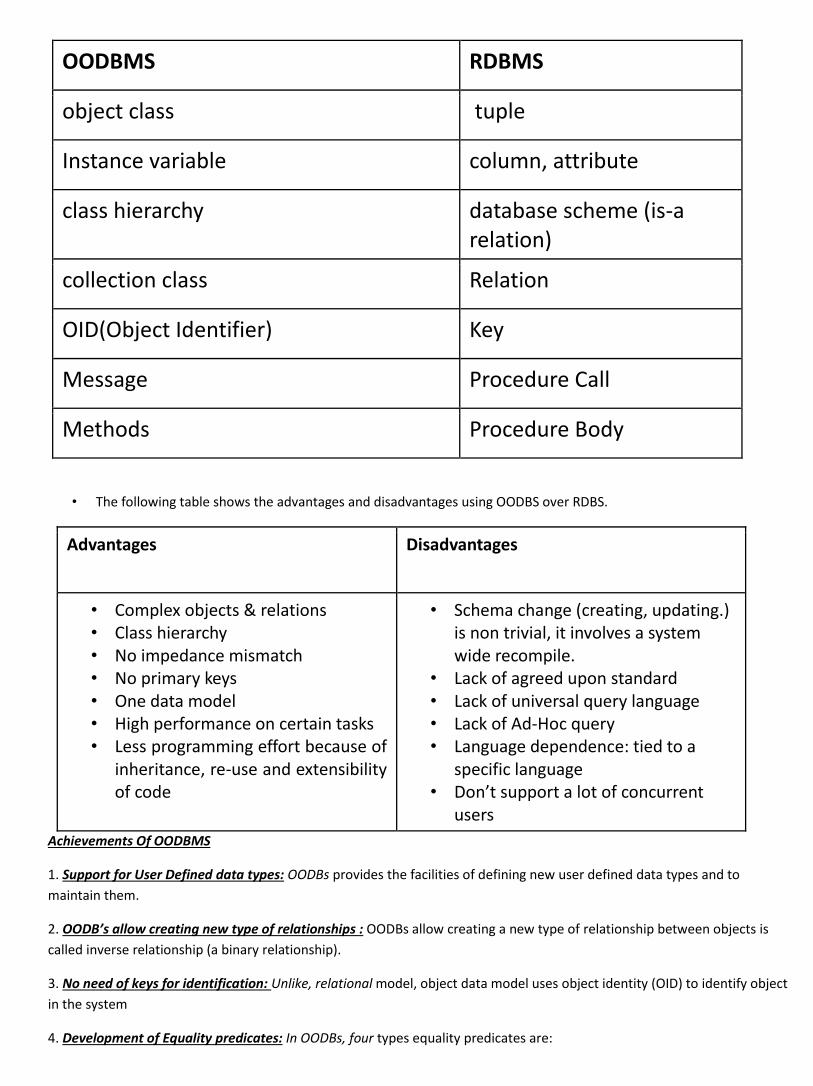
OODBMS RDBMS
object class tuple
Instance variable column, attribute
class hierarchy database scheme (is-a relation)
collection class Relation
OID(Object Identifier) Key
Message Procedure Call
Methods Procedure Body
• The following table shows the advantages and disadvantages using OODBS over RDBS.
Advantages Disadvantages
• Complex objects & relations • Class hierarchy
• No impedance mismatch
• No primary keys • One data model • High performance on certain tasks • Less programming effort because of
inheritance, re-use and extensibility of code
• Schema change (creating, updating.) is non trivial, it involves a system wide recompile.
• Lack of agreed upon standard
• Lack of universal query language
• Lack of Ad-Hoc query
• Language dependence: tied to a specific language
• Don’t support a lot of concurrent users
Achievements Of OODBMS
1. Support for User Defined data types: OODBs provides the facilities of defining new user defined data types and to
maintain them.
2. OODB’s allow creating new type of relationships : OODBs allow creating a new type of relationship between objects is
called inverse relationship (a binary relationship).
3. No need of keys for identification: Unlike, relational model, object data model uses object identity (OID) to identify object
in the system
4. Development of Equality predicates: In OODBs, four types equality predicates are:

• Identity equality
• Value equality of objects
• Value equality of properties
• Identity equality of properties
5. No need of joins for OODBMS’s: OODBs has ability to reduce the need of joins .
6. Performance gains over RDBMS: Performance gains changes application to application. Applications that make the use of
object identity concept having performance gains over RDBMS’s.
7. Provide Facility for versioning management: The control mechanisms are missing in most of the RDBMS’s, but it is
supported by the OODBMS’s .
8. Support for nested and long Duration transactions: Most of the RDBMS’s do not support for long and nested transactions,
but OODBMS’s support for nested and long duration transactions.
9. Development of object algebra: Relational algebra is based on relational mathematics and fully implemented, but object
algebra has not been defined in proper way. Five fundamental object preserving operators are: union, difference, select,
generate and map.
Drawbacks Of OODBMS
1. Coherency between Relational and Object Model: Relational databases are founded in every organization. To overcome
relational databases, object databases have to be providing coherent services to users to migrate from relational database to
object database. Architecture of Relational model and Object model must be provide some coherency between them [9].
2. Optimization of Query Expression: Query expression optimization is done to increase the performance of the system
Optimization of queries is very important for performance gains. But due to following reasons it is difficult to optimize
queries in object databases:
• User defined data types
• Changing variety of types
• Complex objects, methods and encapsulation
• Object Query language has nested structure
• Object Identity
3. No fixed query algebra for OODBMS’s: Due to lack of the standards in OODBMS, there is no standard query algebra for
OODB. Lack of standard query algebra becomes one of the reasons for problem of query optimization. There are different
query languages for different object databases.
4. No full-fledged query system: Query system also not fully implemented. Some query facilities lacks in Object databases
like nested sub-queries, set queries and aggregation function.
5. No facility for Views: In relational databases, views are temporary tables. Object databases having no facility for views. An
object oriented view capability is difficult to implement due to the features of Object Model such as object identity. Object
oriented programming concepts like inheritance and encapsulation makes the difficult to implement views in object
databases.

6. Security problems in Object databases: Security is related to authentication, authorization and accounting. Discretionary
Access Control (DAC), Mandatory Access Control (MAC) security policies are implemented in object databases to secure data.
In some systems provide security on the basis of object oriented concepts like encapsulation. Object database having to
facilities for authorization.
A schema is a collection of logical structures of data, or schema objects. A schema is owned by a
database user and has the same name as that user. Each user owns a single schema. Schema objects can
be created and manipulated with SQL and include the following types of objects:
Clusters
Database links
Database triggers
Dimensions
External procedure libraries
Indexes and index types
Java classes, Java resources, and Java sources
Materialized views and materialized view logs
Object tables, object types, and object views
Operators
Sequences
Stored functions, procedures, and packages
Synonyms
Tables and index-organized tables
Views
Other types of objects are also stored in the database and can be created and manipulated with SQL but
are not contained in a schema:
Contexts
Directories
Profiles
Roles
Tablespaces
Users
Rollback segments
Schema objects are logical data storage structures. Schema objects do not have a one-to-one
correspondence to physical files on disk that store their information. However, Oracle stores a schema
object logically within a tablespace of the database. The data of each object is physically contained in
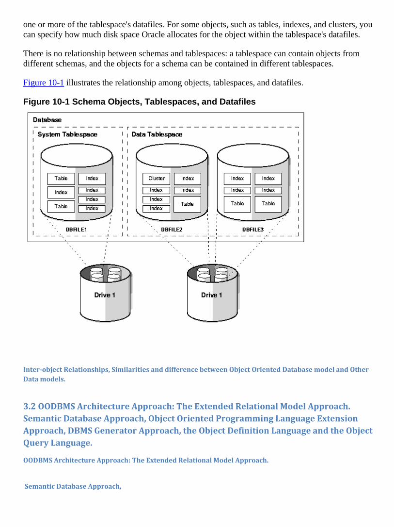
one or more of the tablespace's datafiles. For some objects, such as tables, indexes, and clusters, you
can specify how much disk space Oracle allocates for the object within the tablespace's datafiles.
There is no relationship between schemas and tablespaces: a tablespace can contain objects from
different schemas, and the objects for a schema can be contained in different tablespaces.
Figure 10-1 illustrates the relationship among objects, tablespaces, and datafiles.
Figure 10-1 Schema Objects, Tablespaces, and Datafiles
Inter-object Relationships, Similarities and difference between Object Oriented Database model and Other
Data models.
3.2 OODBMS Architecture Approach: The Extended Relational Model Approach.
Semantic Database Approach, Object Oriented Programming Language Extension
Approach, DBMS Generator Approach, the Object Definition Language and the Object
Query Language.
OODBMS Architecture Approach: The Extended Relational Model Approach.
Semantic Database Approach,
Object Oriented Programming Language Extension Approach,
DBMS Generator Approach,
the Object Definition Language and the Object Query Language.
3.3 The Object Oriented DBMS Architecture, Performance Issue in Object Oriented
DBMS, Application Selection for Object Oriented DBMS, the Database Design for an
Object Relational DBMS. The Structured Typed and ADTs, Object identity, Extending
the ER Model ,Storage and Access Methods, Query Processing Query Optimization, Data
Access API(ODBC,DB Library, DAO,ADO,JDBC,OLEDB), Distributed Computing Concept
in COM, COBRA.
The Object Oriented DBMS Architecture,

The very popular ANSI/SPARC architecture [1] gives three levels that drive the data access and management of a database. These three
levels are external, conceptual, and the internal. The external level consists of particular views of data dedicated to particular client
applications or particular users. In relational databases the external level implements two kinds of facilities: access privileges to particular
resources grated by database administrator to particular users. The SQL views that customize encapsulated and restrict resources to be
accessed. This approach has proven to be enough simple and satisfactory for majority of applications of relational databases. The
conceptual level is common for the entire database environment. In this level the storage structure of data is defined. The Internal of
Physical level describes the physical storage of data on secondary device.
But the situation is different in object oriented database, the complex structure data is managed by object oriented database. Piotr
Habela1 et. al. [2] provides foundation for three-level database architecture and correspondingly three database development roles: (1)
a database programmer defines stored objects, i.e. their state and behavior; (2) a database administrator (DBA) creates views and
interfaces which encapsulate stored objects and possibly limit access rights on them; (3) an application programmer or a user
receives access and updating grants from DBA in the form of interfaces to views. They present a concrete solution that they developed as a
platform for grid and Web applications.
The problem how to efficiently store, retrieve, analyze and modify the biological data and multimedia data are
becoming an important issue for most biological scientists and computer scientists who is working in the field of multimedia data
manipulation. In order to solve this problem, a Domain Specific Object Oriented Data Base Management System (DSOODBMS) is
designed to manipulate Protein Data that is biological data, Yanchao Wang et. al.[3]. They have designed special architecture for the
protein data in object oriented databases.
Muhammad Ubaid et al.[4] have describe in their paper that the object oriented techniques may include features such as encapsulation,
modularity, polymorphism, and inheritance, for implementing this paradigm. They suggested that there should be a good architecture
design of classes’ schema for the OODBM system that could help to maintain the relationship between the objects and fulfill the core
concept of the object oriented. When we are storing the data as object in OODBMS than OODBMS maintain the Object Identity (OID) and
the identity of an object has an existence independent of the values of the object attributes, Elisa Bertino et. al. [5].
2. 2. Architecture design issues for OODBMS The architecture play important role in database system to manage the data. The architecture design decisions concern the rules for data
transfer from database server to client and client to database server, vice versa. The error handling is also important issue while transferring
data
between user and machine. The machine is consisting with physical devices. The error may
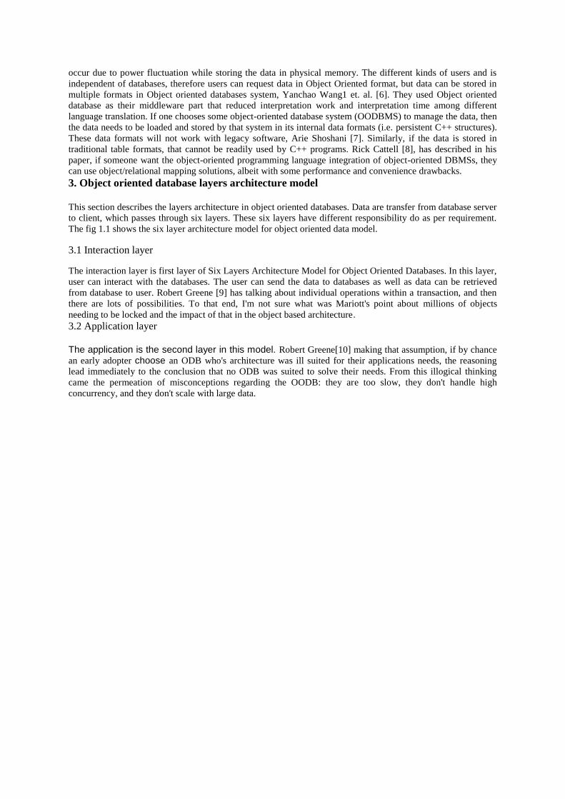
occur due to power fluctuation while storing the data in physical memory. The different kinds of users and is
independent of databases, therefore users can request data in Object Oriented format, but data can be stored in
multiple formats in Object oriented databases system, Yanchao Wang1 et. al. [6]. They used Object oriented
database as their middleware part that reduced interpretation work and interpretation time among different
language translation. If one chooses some object-oriented database system (OODBMS) to manage the data, then
the data needs to be loaded and stored by that system in its internal data formats (i.e. persistent C++ structures).
These data formats will not work with legacy software, Arie Shoshani [7]. Similarly, if the data is stored in
traditional table formats, that cannot be readily used by C++ programs. Rick Cattell [8], has described in his
paper, if someone want the object-oriented programming language integration of object-oriented DBMSs, they
can use object/relational mapping solutions, albeit with some performance and convenience drawbacks.
3. Object oriented database layers architecture model This section describes the layers architecture in object oriented databases. Data are transfer from database server
to client, which passes through six layers. These six layers have different responsibility do as per requirement.
The fig 1.1 shows the six layer architecture model for object oriented data model.
3.1 Interaction layer
The interaction layer is first layer of Six Layers Architecture Model for Object Oriented Databases. In this layer,
user can interact with the databases. The user can send the data to databases as well as data can be retrieved
from database to user. Robert Greene [9] has talking about individual operations within a transaction, and then
there are lots of possibilities. To that end, I'm not sure what was Mariott's point about millions of objects
needing to be locked and the impact of that in the object based architecture.
3.2 Application layer
The application is the second layer in this model. Robert Greene[10] making that assumption, if by chance
an early adopter choose an ODB who's architecture was ill suited for their applications needs, the reasoning
lead immediately to the conclusion that no ODB was suited to solve their needs. From this illogical thinking
came the permeation of misconceptions regarding the OODB: they are too slow, they don't handle high
concurrency, and they don't scale with large data.
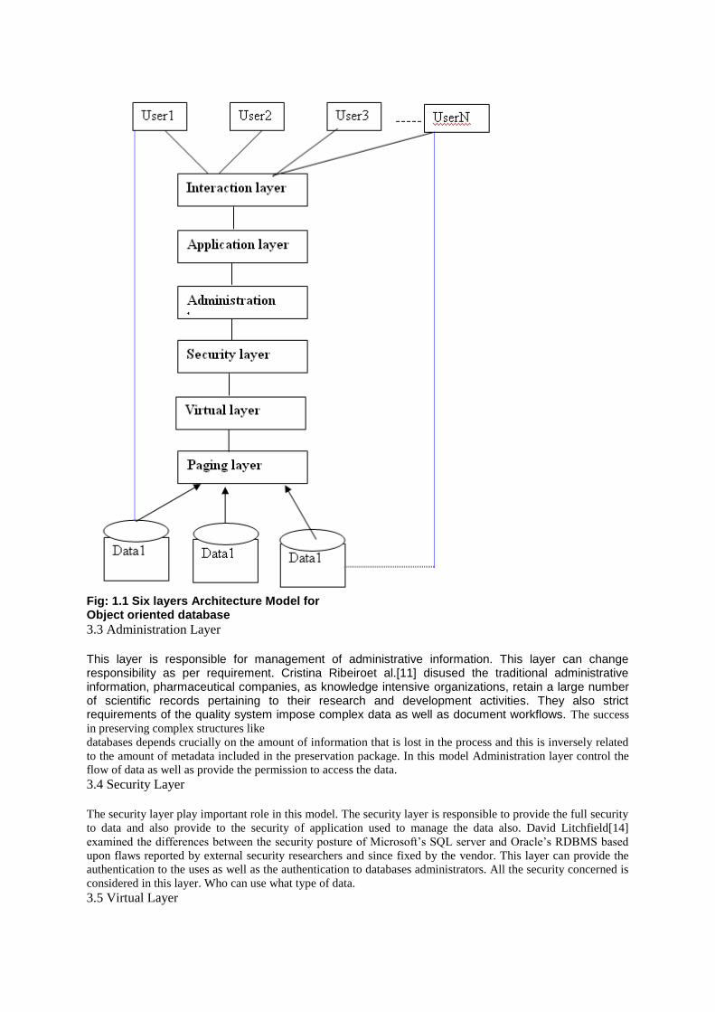
Fig: 1.1 Six layers Architecture Model for Object oriented database
3.3 Administration Layer
This layer is responsible for management of administrative information. This layer can change responsibility as per requirement. Cristina Ribeiroet al.[11] disused the traditional administrative information, pharmaceutical companies, as knowledge intensive organizations, retain a large number of scientific records pertaining to their research and development activities. They also strict requirements of the quality system impose complex data as well as document workflows. The success
in preserving complex structures like
databases depends crucially on the amount of information that is lost in the process and this is inversely related
to the amount of metadata included in the preservation package. In this model Administration layer control the
flow of data as well as provide the permission to access the data.
3.4 Security Layer
The security layer play important role in this model. The security layer is responsible to provide the full security
to data and also provide to the security of application used to manage the data also. David Litchfield[14]
examined the differences between the security posture of Microsoft’s SQL server and Oracle’s RDBMS based
upon flaws reported by external security researchers and since fixed by the vendor. This layer can provide the
authentication to the uses as well as the authentication to databases administrators. All the security concerned is
considered in this layer. Who can use what type of data.
3.5 Virtual Layer
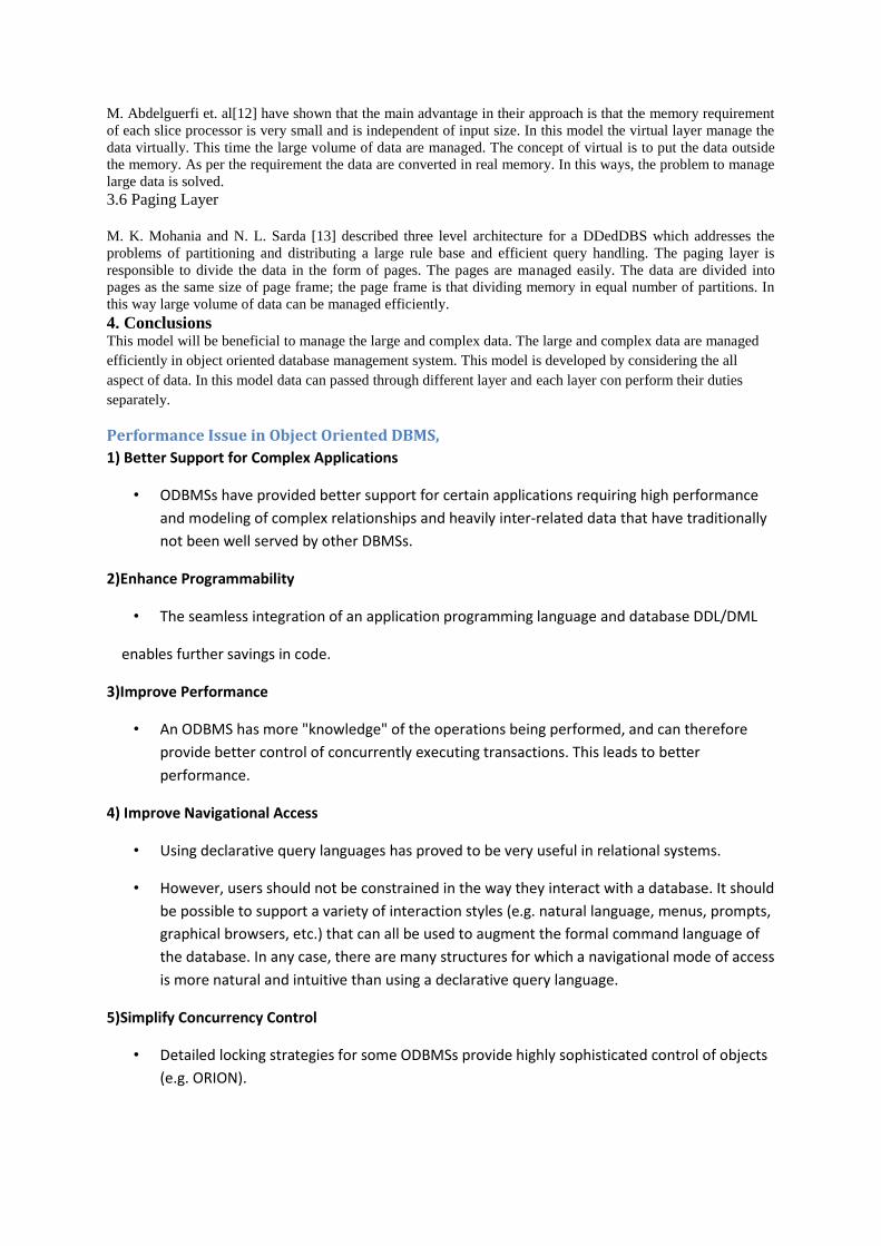
M. Abdelguerfi et. al[12] have shown that the main advantage in their approach is that the memory requirement
of each slice processor is very small and is independent of input size. In this model the virtual layer manage the
data virtually. This time the large volume of data are managed. The concept of virtual is to put the data outside
the memory. As per the requirement the data are converted in real memory. In this ways, the problem to manage
large data is solved.
3.6 Paging Layer
M. K. Mohania and N. L. Sarda [13] described three level architecture for a DDedDBS which addresses the
problems of partitioning and distributing a large rule base and efficient query handling. The paging layer is
responsible to divide the data in the form of pages. The pages are managed easily. The data are divided into
pages as the same size of page frame; the page frame is that dividing memory in equal number of partitions. In
this way large volume of data can be managed efficiently.
4. Conclusions This model will be beneficial to manage the large and complex data. The large and complex data are managed
efficiently in object oriented database management system. This model is developed by considering the all
aspect of data. In this model data can passed through different layer and each layer con perform their duties
separately.
Performance Issue in Object Oriented DBMS,
1) Better Support for Complex Applications
• ODBMSs have provided better support for certain applications requiring high performance
and modeling of complex relationships and heavily inter-related data that have traditionally
not been well served by other DBMSs.
2)Enhance Programmability
• The seamless integration of an application programming language and database DDL/DML
enables further savings in code.
3)Improve Performance
• An ODBMS has more "knowledge" of the operations being performed, and can therefore
provide better control of concurrently executing transactions. This leads to better
performance.
4) Improve Navigational Access
• Using declarative query languages has proved to be very useful in relational systems.
• However, users should not be constrained in the way they interact with a database. It should
be possible to support a variety of interaction styles (e.g. natural language, menus, prompts,
graphical browsers, etc.) that can all be used to augment the formal command language of
the database. In any case, there are many structures for which a navigational mode of access
is more natural and intuitive than using a declarative query language.
5)Simplify Concurrency Control
• Detailed locking strategies for some ODBMSs provide highly sophisticated control of objects
(e.g. ORION).

• At a coarse level of granularity, it is possible to place a single lock on an entire object
hierarchy.
• In contrast, an RDBMS would require multiple locks to get information from related but
scattered data in the database.
• At a fine level of granularity, individual objects or attributes of objects could be locked.
6) Reduce Problems of Referential Integrity
• One of the major problems with relational databases has been that of dangling references.
• This problem has been solved in object databases by giving the responsibility of pointer
maintenance to the database itself, rather than to each application.
7) Abstraction Gain
• The object paradigm provides a better modeling framework that captures not only data and
behavior, but raises the level of abstraction (an object is more
than the sum of its attributes and methods).
Application Selection for Object Oriented DBMS,
• Basically, an OODBMS is an object database that provides DBMS capabilities to objects that
have been created using an object-oriented programming language (OOPL).
• The basic principle is to add persistence to objects and to make objects persistent.
• Consequently application programmers who use OODBMSs typically write programs in a
native OOPL such as Java, C++ or Smalltalk, and the language has some kind of Persistent
class, Database class, Database Interface, or Database API that provides DBMS functionality
as, effectively, an extension of the OOPL.
• Object-oriented DBMSs, therefore, support advanced object-oriented database applications
with features like support for persistent objects from more than one programming language,
distribution of data, advanced transaction models, versions, schema evolution, and dynamic
generation of new types.
• In today's world, Client-Server applications that rely on a database on the server as a data
store while servicing requests from multiple clients are quite commonplace.
• Most of these applications use a Relational Database Management System (RDBMS) as their
data store while using an object oriented programming language for development.
• This causes a certain inefficency as objects must be mapped to tuples in the database and
vice versa instead of the data being stored in a way that is consistent with the programming
model.
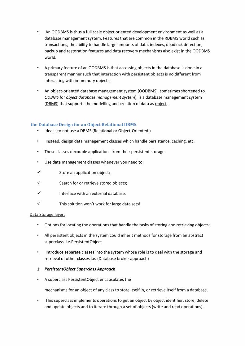
• An OODBMS is thus a full scale object oriented development environment as well as a
database management system. Features that are common in the RDBMS world such as
transactions, the ability to handle large amounts of data, indexes, deadlock detection,
backup and restoration features and data recovery mechanisms also exist in the OODBMS
world.
• A primary feature of an OODBMS is that accessing objects in the database is done in a
transparent manner such that interaction with persistent objects is no different from
interacting with in-memory objects.
• An object-oriented database management system (OODBMS), sometimes shortened to
ODBMS for object database management system), is a database management system
(DBMS) that supports the modelling and creation of data as objects.
the Database Design for an Object Relational DBMS.
• Idea is to not use a DBMS (Relational or Object-Oriented.)
• Instead, design data management classes which handle persistence, caching, etc.
• These classes decouple applications from their persistent storage.
• Use data management classes whenever you need to:
Store an application object;
Search for or retrieve stored objects;
Interface with an external database.
This solution won’t work for large data sets!
Data Storage layer:
• Options for locating the operations that handle the tasks of storing and retrieving objects:
• All persistent objects in the system could inherit methods for storage from an abstract
superclass i.e.PersistentObject
• Introduce separate classes into the system whose role is to deal with the storage and
retrieval of other classes i.e. (Database broker approach)
1. PersistentObject Superclass Approach
• A superclass PersistentObject encapsulates the
mechanisms for an object of any class to store itself in, or retrieve itself from a database.
• This superclass implements operations to get an object by object identifier, store, delete
and update objects and to iterate through a set of objects (write and read operations).

2. Database Broker Approach
• Each persistent class could be responsible for its own storage...but
highly coupled (to storage mechanism);
lessens class cohesion;
class must now have expert knowledge of storage tasks;
these are unrelated to application tasks.
• Separates the business objects from their data storage implementation.
• The classes that provide the data storage services will be held in a separate package.
• For each business class that needs to be persistent, there will be an associated database
broker class.
The Broker Class:
• The broker class provides the mechanisms to materialize objects from the database and
dematerialize them back to the database.
The Database Broker:
• The database broker object is responsible for:
“materialising” objects,
“dematerialising” objects,
caching objects.
• Application classes are insulated from storage.
• Allows migration of storage sub-systems, e.g., implement on existing relational system.
• Replace this with OODBMS.
• Application programs unaffected by change.
Caching Objects
• Objects can be cached for efficiency.
• The cache is a collection maintained by the database broker.
• When an object is requested, the cache is searched first.
• If the object sought is not in the cache it is materialised by the database broker from the
database.
Collections

• In systems where collection classes are used in design, these
may be replaced by database broker objects.
• Database objects provide collection-like services for large volumes of data (more than you
would maintain in a collection
class in memory).
The Structured Typed and ADTs, Object identity,
Object identifier
• An object is defined by a triple (OID, type constructor, state) where OID is the unique object
identifier, type constructor is its type (such as atom, tuple, set, list, array, bag, etc.) and state
is its actual value.
• Example:
(i1, atom, 'John')
(i2, atom, 30)
• An object has structure or state (variables) and methods (behavior/operations)
• An object is described by four characteristics
Identifier: a system-wide unique id for an object
Name: an object may also have a unique name in DB (optional)
Lifetime: determines if the object is persistent or transient
Structure: Construction of objects using type constructors
Using an oid to refer to an object is similar to using a foreign key to refer to a record in another
relation, but not quiet the same:
• An oid can point to an object of theater_t that is stored anywhere in the database, even in a
field
• Whereas a foreign key reference is constrained to point to an object in a particular
reference relation.
Extending the ER Model ,
Storage and Access Methods,
• The main purpose of a DBMS was to centralize and organize data storage. A DBMS program
ran on a single, large machine.
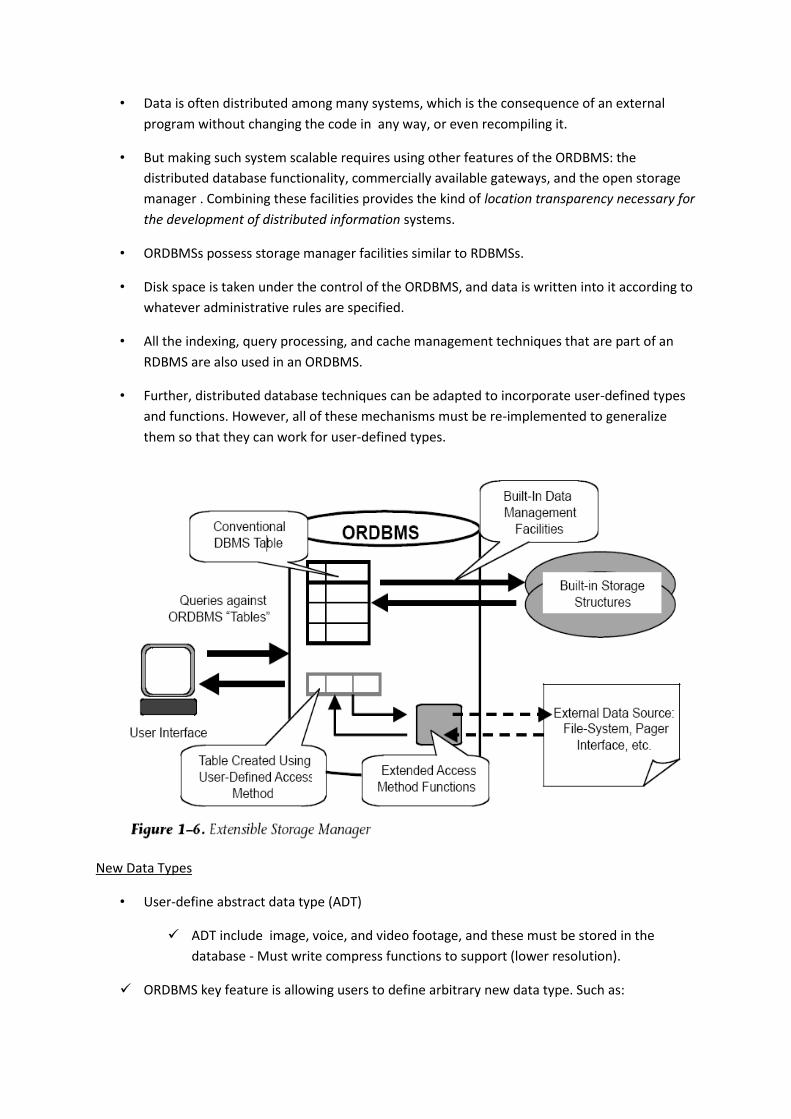
• Data is often distributed among many systems, which is the consequence of an external
program without changing the code in any way, or even recompiling it.
• But making such system scalable requires using other features of the ORDBMS: the
distributed database functionality, commercially available gateways, and the open storage
manager . Combining these facilities provides the kind of location transparency necessary for
the development of distributed information systems.
• ORDBMSs possess storage manager facilities similar to RDBMSs.
• Disk space is taken under the control of the ORDBMS, and data is written into it according to
whatever administrative rules are specified.
• All the indexing, query processing, and cache management techniques that are part of an
RDBMS are also used in an ORDBMS.
• Further, distributed database techniques can be adapted to incorporate user-defined types
and functions. However, all of these mechanisms must be re-implemented to generalize
them so that they can work for user-defined types.
New Data Types
• User-define abstract data type (ADT)
ADT include image, voice, and video footage, and these must be stored in the
database - Must write compress functions to support (lower resolution).
ORDBMS key feature is allowing users to define arbitrary new data type. Such as:

• compress, rotate, shrink and crop
Combination of an atomic data type and its associated methods is called: Abstract
data type (ADT). Such object-relational systems, user allows to include ADT.
• Structured types
• In this application, as needed in many traditional business data processing
applications, we need new types built up from atomic types using constructors for
creating sets, records, arrays, sequences, and so on..
• Structured types
ROW
A type representing a row, or record, of n field with fields n of type n….etc
Listof(base)
Type representing a sequence of base-type items
Array(base)
A type representing an array of base-type items
Setof(base)
A type representing a set of base-type items. Sets cannot contain duplicate elements.
bagof(base)
A type resenting a bag or multiset of based-type items
Query Processing
• It was commonly believed that the application domains that OODBMS technology
targets do not need querying capabilities.
• The issues related to the optimization and execution of OODBMS query languages
which we collectively call query processing.
Query Optimization,
Query Processing Architecture
two architectural issues:
• the query processing methodology and
• the query optimizer architecture.

Query Processing Methodology
• A query processing methodology similar to relational DBMSs, but modified to deal with the
difficulties can be followed in OODBMSs.
Steps of methodology are
• Queries are expressed in a declarative language which requires no user knowledge of object
implementations, access paths or processing strategies.
• The calculus expression is first reduced to a normalized form by eliminating duplicate
predicates, applying identities and rewriting.
• The normalized expression is then converted to an equivalent object algebra expression.
• This form of the query is a nested expression which can be viewed as a tree whose nodes
are algebra operators and whose leaves represent extents of classes in the database.
• The algebra expression is next checked for type consistency to insure that predicates and
methods are not applied to objects which do not support the requested functions.
• This is not as simple as type checking in general programming languages since intermediate
results, which are sets of objects, may be composed of heterogeneous types.
• The next step in query processing is the application of equivalence-preserving rewrite rules
to the type consistent algebra expression. Lastly, an execution plan which takes into account
object implementations is generated from the optimized algebra expression.
Optimizer Architecture
• Query optimization can be modeled as an optimization problem whose solution is the choice
of the “optimum” state in a state space (also called search space). In query optimization,
each state corresponds to an algebraic query indicating an execution schedule and
represented as a processing tree.

• The state space is a family of equivalent (in the sense of generating the same result)
algebraic queries.
• Query optimizers generate and search a state space using a search strategy applying a cost
function to each state and finding one with minimal cost1.
Thus, to characterize a query optimizer three things need to be specified:
1. the search space and the the transformation rules that generate the alternative query
expressions which constitute the search space;
2. a search algorithm that allows one to move from one state to another in the search space;
and
3. the cost function that is applied to each state.
Optimization Techniques
The optimization techniques for object queries follows two fundamental directions.
1. The first is the cost-based optimization of queries based on algebraic manipulations.
Algebraic optimization techniques have been studied quite extensively within the context of
the relational model.
2. The second is the optimization of path expressions.
Path expressions represent traversal paths between objects and are unique to OODBMSs.
The optimization of path expressions is an important issue in OODBMSs and has been a subject of
considerable investigation.
1. Algebraic Optimization
Search Space and Transformation Rules
Search Algorithm
Cost Function
Parameterization
2. Path Expressions
Rewriting
Algebraic optimization
Path indexes

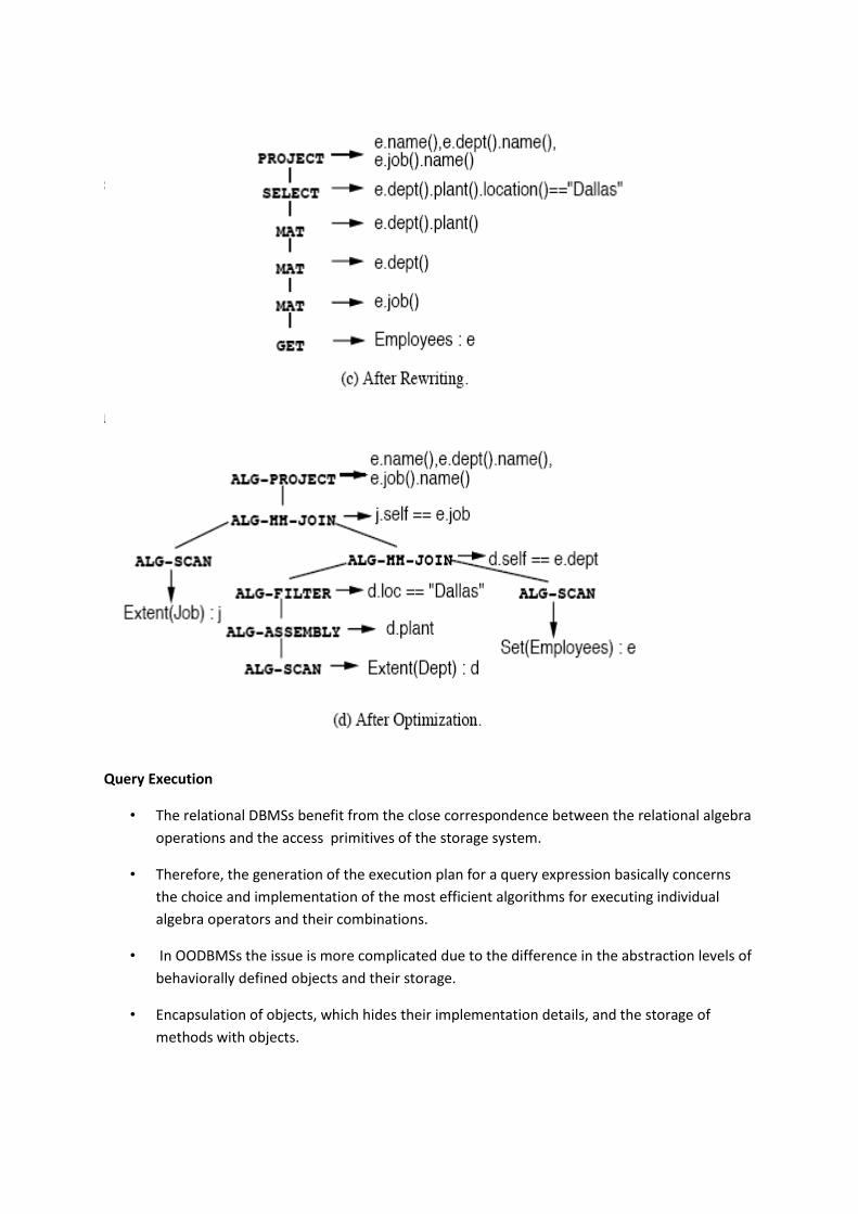
Query Execution
• The relational DBMSs benefit from the close correspondence between the relational algebra
operations and the access primitives of the storage system.
• Therefore, the generation of the execution plan for a query expression basically concerns
the choice and implementation of the most efficient algorithms for executing individual
algebra operators and their combinations.
• In OODBMSs the issue is more complicated due to the difference in the abstraction levels of
behaviorally defined objects and their storage.
• Encapsulation of objects, which hides their implementation details, and the storage of
methods with objects.

• A query-execution engine requires three basic classes of algorithms on collections of objects:
(collection) scan, indexed scan, and collection matching. Collection scan is a straightforward
algorithm that sequentially accesses all objects in a collection.
Data Access API(ODBC,DB Library, DAO,ADO,JDBC,OLEDB),
ODBC
• Open Database Connectivity (ODBC) is a standard application programming interface (API)
for accessing database management systems (DBMS). The designers of ODBC aimed to make
it independent of database systems and operating systems.
• An application written using ODBC can be ported to other platforms, both on the client and
server side, with few changes to the data access code.
• ODBC accomplishes DBMS independence by using an ODBC driver as a translation layer
between the application and the DBMS.
• The application uses ODBC functions through an ODBC driver manager with which it is
linked, and the driver passes the query to the DBMS.
• ODBC provides a vendor-independent database-access API. The ODBC API has been wildly
successful as a database-access standard. Virtually all products that require database access
support it, and the most recent ODBC driver supports the SQL Server 7.0 enhancements. You
use a call-level interface (CLI) to implement the ODBC API.
ODBC(Components of odbc)
• ODBC API
A library of function calls, a set of error codes, and a standard SQL syntax for accessing data
on DBMSs.
• ODBC Driver Manager
A dynamic-link library (Odbc32.dll) that loads ODBC database drivers on behalf of an
application. This DLL is transparent to your application.
• ODBC database drivers
One or more DLLs that process ODBC function calls for specific DBMSs. For a list of supplied
drivers, see ODBC Driver List.
• ODBC Cursor Library
A dynamic-link library (Odbccr32.dll) that resides between the ODBC Driver Manager and the
drivers and handles scrolling through the data.
• ODBC Administrator
A tool used for configuring a DBMS to make it available as a data source for an application.
Db library
• DB-Library provides source code compatibility for older Sybase applications. Sybase
encourages programmers to implement new applications with Client-Library or Embedded
SQL.
• DB-Library/C includes C routines and macros that allow an application to interact with
Adaptive Server and Open Server applications.
• It includes routines that send commands to Adaptive Server and Open Server applications
and others that process the results of those commands. Other routines handle error
conditions, perform data conversion, and provide a variety of information about the
application’s interaction with a server.
• DB-Library/C also contains several header files that define structures and values used by the
routines. Versions of DB-Library have been developed for a number of languages besides C,
including COBOL, FORTRAN, Ada, and Pascal.
DAO(Data Access Objects)
• In computer software, a data access object (DAO) is an object that provides an abstract
interface to some type of database or other persistence mechanism.
• By mapping application calls to the persistence layer, the DAO provides some specific data
operations without exposing details of the database.
• This isolation supports the Single responsibility principle. It separates what data access the
application needs, in terms of domain-specific objects and data types (the public interface of
the DAO), from how these needs can be satisfied with a specific DBMS, database schema,
etc. (the implementation of the DAO).
• it is traditionally associated with Java EE applications and with relational databases
(accessed via the JDBC API )
• The advantage of using data access objects is the relatively simple and rigorous separation
between two important parts of an application that can but should not know anything of
each other, and which can be expected to evolve frequently and independently.
• Changing business logic can rely on the same DAO interface, while changes to persistence
logic do not affect DAO clients as long as the interface remains correctly implemented. All
details of storage are hidden from the rest of the application (information hiding).
• DAOs act as an intermediary between the application and the database. They move data
back and forth between objects and database records.
JDBC(Java database connectivity)
• The Java Database Connectivity (JDBC) API is the industry standard for database-
independent connectivity between the Java programming language and a wide range of
databases – SQL databases and other tabular data sources, such as spreadsheets or flat files.
The JDBC API provides a call-level API for SQL-based database access.
• JDBC technology allows you to use the Java programming language to exploit "Write Once,
Run Anywhere" capabilities for applications that require access to enterprise data. With a
JDBC technology-enabled driver, you can connect all corporate data even in a
heterogeneous environment.
Oledb
• OLE DB (Object Linking and Embedding, Database, sometimes written as OLEDB or OLE-DB),
an API designed by Microsoft, allows accessing data from a variety of sources in a uniform
manner. The API provides a set of interfaces implemented using the Component Object
Model (COM); it is otherwise unrelated to OLE. Microsoft originally intended OLE DB as a
higher-level replacement for, and successor to, ODBC, extending its feature set to support a
wider variety of non-relational databases, such as object databases and spreadsheets that
do not necessarily implement SQL.
• OLE DB is Microsoft's strategic low-level application program interface for access to different
data sources. OLE DB includes not only the Structured Query Language capabilities of the
Microsoft-sponsored standard data interface Open Database Connectivity but also includes
access to data other than SQL data.
Distributed Computing Concept in COM, COBRA.
What is COM?
• Microsoft COM (Component Object Model) technology in the Microsoft Windows-family of
Operating Systems enables software components to communicate. COM is used by
developers to create re-usable software components, link components together to build
applications, and take advantage of Windows services. COM objects can be created with a
variety of programming languages. Object-oriented languages, such as C++, provide
programming mechanisms that simplify the implementation of COM objects. The family of
COM technologies includes COM+, Distributed COM (DCOM) and ActiveX® Controls.
• Microsoft provides COM interfaces for many Windows application programming interfaces
such as Direct Show, Media Foundation, Packaging API, Windows Animation Manager,
Windows Portable Devices, and Microsoft Active Directory (AD).
• COM is used in applications such as the Microsoft Office Family of products.
What is CORBA?
• The Common Object Request Broker Architecture (CORBA) is a standard developed by the
Object Management Group (OMG) to provide interoperability among distributed objects.
• CORBA is the world's leading middleware solution enabling the exchange of information,
independent of hardware platforms, programming languages, and operating systems.
• CORBA is essentially a design specification for an Object Request Broker (ORB), where an
ORB provides the mechanism required for distributed objects to communicate with one
another, whether locally or on remote devices, written in different languages, or at different
locations on a network.
• CORBA is often described as a "software bus" because it is a software-based
communications interface through which objects are located and accessed.
• Using CORBA, application components can communicate with one another no matter where
they are located, or who has designed them. CORBA provides the location transparency to
be able to execute these applications.
• In order to build a system that uses or implements a CORBA-based distributed object
interface, a developer must either obtain or write the IDL code that defines the object-
oriented interface to the logic the system will use or implement.
• Typically, an ORB implementation includes a tool called an IDL compiler that translates the
IDL interface into the target language for use in that part of the system.
• A traditional compiler then compiles the generated code to create the linkable-object files
for use in the application.
• One of the benefits of using CORBA to implement a system such as our shopping cart
application is that the objects can be accessed by services written in different languages.
• To accomplish this task, CORBA defines an interface to which all languages must conform.
• The CORBA interface is called the Interface Definition Language (IDL).
• For CORBA to work, both sides of the wire, the client and server, must adhere to the
contract as stated in the IDL.
• The main premise of CORBA (Common Object Request Broker Architecture) is this: Using a
standard protocol,CORBA allows programs from different vendors to communicate with
each other.This interoperability covers hardware and software.Thus, vendors can write
applications on various hardware platforms and operating systems using a wide variety of
programming languages, operating over different vendor networks.