UNIFYING AMPLITUDE AND PHASE ANALYSIS: A ... · a functional principal component analysis, ......
49
UNIFYING AMPLITUDE AND PHASE ANALYSIS: A COMPOSITIONAL DATA APPROACH TO FUNCTIONAL MULTIVARIATE MIXED-EFFECTS MODELING OF MANDARIN CHINESE P. Z. HADJIPANTELIS 1,2 , J. A. D. ASTON 1,3 , H. G. M ¨ ULLER 4 AND J. P. EVANS 5 1 CENTRE FOR RESEARCH IN STATISTICAL METHODOLOGY, UNIVERSITY OF WARWICK 2 CENTRE FOR COMPLEXITY SCIENCE, UNIVERSITY OF WARWICK 3 STATISTICAL LABORATORY, DEPARTMENT OF PURE MATHS AND MATHEMATICAL STATISTICS, UNIVERSITY OF CAMBRIDGE 4 DEPARTMENT OF STATISTICS, UNIVERSITY OF CALIFORNIA, DAVIS 5 INSTITUTE OF LINGUISTICS, ACADEMIA SINICA ABSTRACT. Mandarin Chinese is characterized by being a tonal language; the pitch (or F 0 ) of its utterances carries considerable linguistic information. However, speech samples from different in- dividuals are subject to changes in amplitude and phase which must be accounted for in any analysis which attempts to provide a linguistically meaningful description of the language. A joint model for amplitude, phase and duration is presented which combines elements from Functional Data Analy- sis, Compositional Data Analysis and Linear Mixed Effects Models. By decomposing functions via a functional principal component analysis, and connecting registration functions to compositional data analysis, a joint multivariate mixed effect model can be formulated which gives insights into the relationship between the different modes of variation as well as their dependence on linguistic and non-linguistic covariates. The model is applied to the COSPRO-1 data set, a comprehensive database of spoken Taiwanese Mandarin, containing approximately 50 thousand phonetically diverse sample F 0 contours (syllables), and reveals that phonetic information is jointly carried by both amplitude and phase variation. 1. I NTRODUCTION Mandarin Chinese is one of the world’s major languages [1] and is spoken as a first language by approximately 900 million people, with considerably more being able to understand it as a Key words and phrases. Phonetic Analysis, Functional Data Analysis, Linguistics, Registration, Multivariate Lin- ear Mixed models. 1 arXiv:1308.0868v4 [stat.AP] 28 Dec 2014
Transcript of UNIFYING AMPLITUDE AND PHASE ANALYSIS: A ... · a functional principal component analysis, ......

UNIFYING AMPLITUDE AND PHASE ANALYSIS:A COMPOSITIONAL DATA APPROACH TO FUNCTIONAL MULTIVARIATE
MIXED-EFFECTS MODELING OF MANDARIN CHINESE
P. Z. HADJIPANTELIS1,2, J. A. D. ASTON1,3, H. G. MULLER4 AND J. P. EVANS5
1CENTRE FOR RESEARCH IN STATISTICAL METHODOLOGY, UNIVERSITY OF WARWICK
2CENTRE FOR COMPLEXITY SCIENCE, UNIVERSITY OF WARWICK
3STATISTICAL LABORATORY, DEPARTMENT OF PURE MATHS AND MATHEMATICAL STATISTICS,
UNIVERSITY OF CAMBRIDGE
4DEPARTMENT OF STATISTICS, UNIVERSITY OF CALIFORNIA, DAVIS
5INSTITUTE OF LINGUISTICS, ACADEMIA SINICA
ABSTRACT. Mandarin Chinese is characterized by being a tonal language; the pitch (or F0) of its
utterances carries considerable linguistic information. However, speech samples from different in-
dividuals are subject to changes in amplitude and phase which must be accounted for in any analysis
which attempts to provide a linguistically meaningful description of the language. A joint model for
amplitude, phase and duration is presented which combines elements from Functional Data Analy-
sis, Compositional Data Analysis and Linear Mixed Effects Models. By decomposing functions via
a functional principal component analysis, and connecting registration functions to compositional
data analysis, a joint multivariate mixed effect model can be formulated which gives insights into the
relationship between the different modes of variation as well as their dependence on linguistic and
non-linguistic covariates. The model is applied to the COSPRO-1 data set, a comprehensive database
of spoken Taiwanese Mandarin, containing approximately 50 thousand phonetically diverse sample
F0 contours (syllables), and reveals that phonetic information is jointly carried by both amplitude
and phase variation.
1. INTRODUCTION
Mandarin Chinese is one of the world’s major languages [1] and is spoken as a first language
by approximately 900 million people, with considerably more being able to understand it as a
Key words and phrases. Phonetic Analysis, Functional Data Analysis, Linguistics, Registration, Multivariate Lin-
ear Mixed models.1
arX
iv:1
308.
0868
v4 [
stat
.AP]
28
Dec
201
4
2 HADJIPANTELIS, ASTON, MULLER & EVANS
secondary language. Spoken Mandarin Chinese, in contrast to most European languages, is a tonal
language [2]. The modulation of the pitch of the sound is an integral part of the lexical identity of
a word. Thus, any statistical approach of Mandarin pitch attempting to provide a pitch typology of
the language, must incorporate the dynamic nature of the pitch contours into the analysis [3, 4].
Pitch contours, and individual human utterances generally, contain variations in both the ampli-
tude and phase of the response, due to effects such as speaker physiology and semantic context.
Therefore, to understand the speech synthesis process and analyze the influence that linguistic (eg.
context) and non-linguistic effects (eg. speaker) have, we need to account for variations of both
types. Traditionally, in many phonetic analyses, pitch curves have been linearly time normalized,
removing effects such as speaker speed or vowel length, and these time normalized curves are sub-
sequently analyzed as if they were the original data [5, 6]. However, this has a major drawback:
potentially interesting information contained in the phase is discarded as pitch patterns are treated
as purely amplitude variational phenomena.
In a philosophically similar way to Kneip and Ramsay [7], we model both phase and amplitude
information jointly and propose a framework for phonetic analysis based on functional data analy-
sis (FDA) [8] and multivariate linear mixed-effects (LME) models [9]. Using a single multivariate
model that concurrently models amplitude, phase and duration, we are able to provide a phonetic
typology of the language in terms of a large number of possible linguistic and non-linguistic effects,
giving rise to estimates that conform directly to observed data. We focus on the dynamics of F0; F0
is the major component of what a human listener identifies as speaker pitch [10] and relates to how
fast the vocal folds of the speaker vibrate [11]. We utilize two interlinked sets of curves; one set
consisting of time normalized F0 amplitude curves and a second set containing their corresponding
time-registration/warping functions registering the original curves to a universal time-scale. Using
methodological results from the compositional data literature [12], a principal component analysis
of the centered log ratio of the time-registration functions is performed. The principal component
scores from the amplitude curves and the time warping functions along with the duration of the
syllable are then jointly modeled through a multivariate LME framework.
UNIFYING AMPLITUDE AND PHASE ANALYSIS 3
One aspect of note in our modeling approach is that it is based on a compositional representation
of the warping functions. This representation is motivated by viewing the registration functions
on normalized time domains as cumulative distribution functions, with derivatives that are density
functions, which in turn can be approximated by histograms arbitrarily closely in the L2 norm.
We may then take advantage of the well-known connection between histograms and compositional
data [13, 14].
The proposed model is applied to a large linguistic corpus of Mandarin Chinese consisting of ap-
proximately 50,000 individual syllables in a wide variety of linguistic and non-linguistic contexts.
Due to the large number of curves, computational considerations are of critical importance to the
analysis. The data set is prohibitively large to analyze with usual multilevel computational im-
plementations [15, 16], so a specific computational approach for the analysis of large multivariate
LME models is developed. Using the proposed model, we are able to identify a joint model for
Mandarin Chinese that serves as a typography for spoken Mandarin. This study thus provides a
robust and flexible statistical framework describing intonation properties of the language.
The paper proceeds as follows. In section 2, a short review of the linguistic properties of Mandarin
will be given. General statistical methodology for the joint modeling of phase and amplitude
functions will then be outlined in section 3, including its relation to compositional data analysis and
other methods of modeling phase and amplitude. Section 4 contains the analysis of the Mandarin
corpus where it will be seen that the model not only provides a method for determining the role
of linguistic covariates in the synthesis of Mandarin, but also allows comparisons between the
estimated and the observed curves. Finally, the last section contains a short discussion of the
future prospects of FDA in linguistics. Further details of the analysis implemented are given in the
Supplementary Material.
2. PHONETIC ANALYSIS OF MANDARIN CHINESE
We focus our attention on modeling fundamental frequency (F0) curves. The amplitude of F0,
usually measured in Hz, quantifies the rate/frequency of the speaker’s vocal folds’ vibration and
is an objective measure of how high or low the speaker’s voice is. In this study, the observation

4 HADJIPANTELIS, ASTON, MULLER & EVANS
0 5 10 15 20 25 30 35 40 45150
200
250
300
Hz
t (10ms)
F0 track segment Tone Sequence 4−5−1
Speaker: F02, Sentence: 530
Original F0 Track
0 5 10 15 20 25 30 35 40 45 50
80
100
120
140
160
180
200
220
Hz
t (10ms)
F0 track segment Tone Sequence 2−1−4
Speaker: M02, Sentence: 106
Original F0 Track
FIGURE 1. An example of triplet trajectories from speakers F02 & M02 over nat-
ural time. F (emale)02 tonal sequence: 4-5-1, M (ale)02 tonal sequence: 2-1-4;
Mandarin Chinese rhyme sequences [oN-@-iou] and [ien-in-ğ] respectively. See Sup-
plementary Material for full contextual covariate information.
units of investigation are brief syllables: F0 segments that typically span between 120 and 210
milliseconds (Figure 1) and are assumed to be smooth and continuous throughout their trajectories.
Linguistically our modeling approach of F0 curves is motivated by the intonation model proposed
by Fujisaki [17] where linguistic, para-linguistic and non-linguistic features are assumed to affect
speaker F0 contours. Another motivation for our rationale of combining phase and amplitude
variation comes from the successful usage of Hidden Markov Models (HMM) [18, 19] in speech
recognition and synthesis modeling. However, unlike the HMM approach, we aim to maintain a
linear modeling framework favored by linguists for its explanatory value [20, 21] and suitability
for statistical modeling.
Usual approaches segment the analysis of acoustic data. First one applies a “standard” Dynamic
Time Warping (DTW) treatment to the sample using templates [22], registers the data in this new
universal time scale and then continues with the analysis of the variational patterns in the syn-
chronized speech utterances [23]. In contrast, we apply Functional Principal Component analysis

UNIFYING AMPLITUDE AND PHASE ANALYSIS 5
(FPCA) [24] to the “warped” F0 curves and also to their corresponding warping functions, the lat-
ter being produced during the curve registration step. These functional principal component scores
then serve as input for using a multivariate LME model, allowing a joint modeling of both the
phase and amplitude variations.
We analyze a comprehensive speech corpus of Mandarin Chinese. The Sinica Continuous Speech
Prosody Corpora (COSPRO) [25] was collected at the Phonetics Lab of the Institute of Linguis-
tics in Academia Sinica and consists of 9 sets of speech corpora. We focus our attention on
the COSPRO-1 corpus; the phonetically balanced speech database. COSPRO-1 was designed to
specifically include all possible syllable combinations in Mandarin based on the most frequently
used 2- to 4-syllable lexical words. Additionally it incorporates all the possible tonal combinations
and concatenations. It therefore offers a high quality speech corpus that, in theory at least, encap-
sulates all the prosodic effects that might be of acoustic interest. Specifically, we analyze 54707
fully annotated “raw” syllabic F0 curves which were uttered by a total of 5 native Taiwanese Man-
darin speakers (two males and three females). Each speaker uttered the same 598 predetermined
sentences having a median length of 20 syllables; each syllable had on average 16 readings.
In total, aside from Speaker and Sentence information, associated with each F0 curve are covari-
ates of break index (within word (B2), intermediate (B3), intonational (B4) and utterance (B5)
segments), its adjacent consonants, its tone and rhyme type (Table 1). In our work all of these
variables serve as potential scalar covariates and with the exception of break counts, the fixed co-
variates are of categorical form. The break (or pause) counts, representing the number of syllables
between successive breaks of a particular type, are initialized at the beginning of the sentence and
are subsequently reset every time a corresponding or higher order break occurs. They represent
the perceived degree of disjunction between any two words, as defined in the ToBi annotations
[26]. Break counts are very significant as physiologically a break has a resetting effect on the vo-
cal folds’ vibrations; a qualitative description of the break counts is provided in the Table 5 of the
Supplementary Material.

6 HADJIPANTELIS, ASTON, MULLER & EVANS
Effects Values Meaning Notation-mark
Fixed effectsprevious tone 0:5 Tone of previous syllable, 0 no previous tone
presenttnprevious
current tone 1:5 Tone of syllable tncurrent
following tone 0:5 Tone of following syllable, 0 no following tonepresent
tnnext
previous consonant 0:3 0 is voiceless, 1 is voiced, 2 not present, 3sil/short pause
cnprevious
next consonant 0:3 0 is voiceless, 1 is voiced, 2 not present, 3sil/short pause
cnnext
B2 linear Position of the B2 index break in sentence B2B3 linear Position of the B3 index break in sentence B3B4 linear Position of the B4 index break in sentence B4B5 linear Position of the B5 index break in sentence B5Sex 0:1 1 for male, 0 for female Sex
Duration linear 10s of ms Duration
rhyme type 1:37 Rhyme of syllable rhymet
Random EffectsSpeaker N(0, σ2
speaker) Speaker Effect SpkrIDSentence N(0,σ2
sentence) Sentence Effect Sentence
TABLE 1. Covariates examined in relation to F0 production in Taiwanese Man-darin. Tone variables in a 5-point scale representing tonal characterization, 5 indi-cating a toneless syllable, with 0 representing the fact that no rhyme precedes thecurrent one (such as at the sentence start). Reference tone trajectories are shown inthe supplementary material section: Linguistic Covariate Information.
3. STATISTICAL METHODOLOGY
3.1. A Joint Model. The application of Functional Data Analysis (FDA) in the field of Pho-
netics, while not wide-spread, is not unprecedented; previous functional data analyzes included
lip-motion [27], analysis of prosodic effects [28], speech production [29] as well as basic language
investigation based solely on amplitude analysis [6]. FDA is, by design, well-suited as a modeling
framework for phonetic samples as F0 curves are expected to be smooth. Concurrent phase and

UNIFYING AMPLITUDE AND PHASE ANALYSIS 7
amplitude variation is expected in linguistic data and as phonetic data sets feature “dense” mea-
surements with high signal to noise ratios [8], FDA naturally emerges as a statistical framework for
F0 modeling. Nevertheless in all phonetic studies mentioned above, the focus of the phonetic anal-
ysis has been almost exclusively the amplitude variations (the size of the features on a function’s
trajectory) rather than the phase variation (the location of the features on a function’s trajectory) or
the interplay between the two domains.
To alleviate the limitation of only considering amplitude, we utilize the formulation presented by
Tang & Muller [30] and introduce two types of functions, wi and hi associated with our observed
curve yi, i = 1, . . . , N where yi is the ith curve in the sample of N curves. For a given F0 curve yi,
wi is the amplitude variation function on the domain [0, 1] while hi is the monotonically increasing
phase variation function on the domain [0, 1], such that hi(0) = 0 and hi(1) = 1. For generic
random phase variation or warping functions h and time domains [0, T ], T also being random,
we consider time transformations u = h−1( tT
) from [0, T ] to [0, 1] with inverse transformations
t = Th(u). Then, the measured curve yi over the interval t ∈ [0, Ti] is assumed to be of the form:
yi(t) = wi(h−1i ( t
Ti))⇔ wi(u) = yi(Tihi(u)), i = 1, . . . , N,(3.1)
where u ∈ [0, 1] and Ti is the duration of the ith curve. A curve yi is viewed as a realization
of the amplitude variation function wi evaluated over u, with the mapping h−1i (·) transforming
the scaled real time t onto the universal/sample-wide time-scale u. In addition, each curve can
depend on a set of covariates, fixed effects Xi, such as the tone being said, and random effects
Zi, where such random effects correspond to additional speaker and context characteristics. While
each individual curve has its own length Ti which is directly observed, the lengths entering the
functional data analysis are normalized and the Ti are subsequently included in the modeling as
part of the multivariate linear mixed effect framework.
In our application, the curves yi are associated with various covariates, for example, tone, speaker,
and sentence position. These are incorporated into the model via the principal component scores
which result from adopting a common principal component approach [31, 32], where we assume

8 HADJIPANTELIS, ASTON, MULLER & EVANS
common principal components (across covariates) for the amplitude functions and another com-
mon set (across covariates) for phase functions (but these two sets can differ). We use a common
PCA framework with common mean and eigenfunctions so that all the variation in both phase and
amplitude is reflected in the respective FPC scores. These ideas have been previously used in a
regression setting (although not in the context of registration) [32, 6, 33]. As will be discussed in
section 4.2, this is not a strong assumption in this application. Of the covariates likely present in
model, tone is known to affect the shape of the curves (indeed it is in the phonetic textual repre-
sentation of the syllable), and therefore the identification of warping functions is carried out within
tone classes as opposed to across the classes as otherwise very strong (artefactual) warpings will
be introduced.
As a direct consequence of our generative model (Eq. (3.1)), wi dictates the size of a given feature
and h−1i dictates the location of that feature for a particular curve i. We assume that wi and hi are
both elements of L2[0, 1]. The wi can be expressed in terms of a basis expansion:
wi(u) = µw(u) +∞∑j=1
Awi,jφj(u),(3.2)
where µw(u) = Ew(u), φj is the jth basis function, and Awi,j is the coefficient for the ith
amplitude curve associated with the jth basis function. The hi are a sample of random distribution
functions which are square integrable but are not naturally representable in a basis expansion in the
Hilbert spaceL2[0, 1], since the space of distribution functions is not closed under linear operations.
A common approach to circumvent this difficulty is to observe that log( dduh(u)) is not restricted
and can be modeled as a basis expansion in L2[0, 1]. A restriction however is that the densities
hi have to integrate to 1, therefore the functions si(u) = log( dduhi(u))) are modeled with the
unrestricted basis expansion:
si(u) = µs(u) +∞∑j=1
Asi,jψj(u),(3.3)
where µs(u), ψk and Asi,j are defined analogously to µw(u), φk and Awi,j respectively, but for the
warping rather than amplitude functions. A transformation step is then introduced to satisfy the
UNIFYING AMPLITUDE AND PHASE ANALYSIS 9
integration condition, which yields the representation:
hi(u) =∫ u
0 esi(u′)du′∫ 1
0 esi(u′)du′
(3.4)
for the warping function hi. Clearly different choices of bases will give rise to different coefficients
A which then can be used for further analysis. A number of different parametric basis functions
can be used as basis; for example Grabe et al. advocate the use of Legendre polynomials [34] for
the modeling of amplitude. We advocate the use of a principal component basis for both wi and
si in Eqs. (3.2) & (3.3), as will be discussed in the next sections, although any basis can be used
in the generic framework detailed here. However, a principal components basis does provide the
most parsimonious basis in terms of a residual sum of squares like criterion [8]. We note that in
order to ensure statistical identifiability of the model (Eq. (3.1)) several regularity assumptions
were introduced in [35, 30], including the exclusion of essentially flat amplitude functions wi
for which time-warping cannot be reasonably identified, and more importantly, assuming that the
time-variation component that is reflected by the random variation in hi and si asymptotically
dominates the total variation. In practical terms, we will always obtain well-defined estimates for
the component representations in Eqs. (3.2) & (3.3), and their usefulness hinges critically on their
interpretability; see section 5.
For our statistical analysis we explicitly assume that each covariate Xi influences, to different
degrees, all of the syllable’s components/modes as well as influencing the syllable’s duration Ti.
Additionally, as mentioned above in accordance with the Fujisaki model, we assume that each
syllable component includes Speaker-specific and Sentence-specific variational patterns; we incor-
porate this information in the covariates Zi. Then the general form of our model for a given sample
curve yi of duration Ti with two sets of scalar covariates Xi and Zi is:
Ewi(u)|Xi, Zi = µw(u) +∞∑j=1
EAwi,j|Xi, Ziφj(u),(3.5)
and
Esi(u)|Xi, Zi = µs(u) +∞∑j=1
EAsi,j|Xi, Ziψj(u).(3.6)

10 HADJIPANTELIS, ASTON, MULLER & EVANS
FunctionalData y
CurveRegistration
Eq. 3.1
AmplitudeFunctions W
Phase Func-tions H
Funct. PCAEq. 3.2
W FPCs: Φ - Fig. 5
W FPC Scores: Aw
CLR Transf.Eq. 3.4
CompositionalRepresentations S
Funct. PCAEq. 3.3
S FPCs: Ψ - Fig. 6
S FPC Scores: As
MVLMEEq. 3.7
Duration T
Aw, As, T
[X,Z]
FIGURE 2. Summary of the overall estimation procedure resulting in the estimates
of the functional principal components and scores via the covariates in the linear
mixed effect model.
Truncating expansions (3.5) and (3.6), to Mw and Ms components respectively, is a computational
necessity and simplifies the implementation. Curves are then reduced to finitely many scores
Awij, Asij and these score vectors then act as surrogate data for curves wi and si. The final joint
model for amplitude, phase and syllable duration is then formulated as:
E[Awi , Asi , Ti]|Xi, Zi = XiB + ZiΓ, Γ ∼ N(0,ΣΓ)(3.7)
where Awi and Asi are the vectors of component coefficients for the i-th sample. Here, B (a k × p
matrix where k is the number of fixed effects in the model and p is the number of multivariate
components in the mixed effects model, p = Mw+Ms+1 where the “1” arises from the additional
duration component in the model) is the parameter matrix of the fixed effects and Γ (a l× p matrix
where l is the number of random effects in the model) contains the coefficients of the random
effects and is assumed to have mean zero, while ΣΓ is the covariance matrix of the amplitude,
phase and duration components with respect to the random effects.
The process as a whole is summarized in Figure 2.
3.2. Amplitude Modeling. In our study, amplitude analysis is conducted through a functional
principal component analysis of the amplitude variation functions. Qualitatively, the random am-
plitude functions wi are the time-registered versions of the original F0 samples. Utilizing FPCA,
we determine the eigenfunctions which correspond to the principal modes of amplitude variation in

UNIFYING AMPLITUDE AND PHASE ANALYSIS 11
the sample and then use a finite number of eigenfunctions corresponding to the largest eigenvalues
as a truncated basis, so that representations in this basis will explain a large fraction of the total
variation. Specifically, we define the kernel Cw of the covariance operator as:
(3.8) Cw(u, u∗) = E(w(u)− µw(u)) (w(u∗)− µw(u∗))
and by Mercer’s theorem [36], the spectral decomposition of the symmetric amplitude covariance
function Cw can be written as:
Cw(u, u∗) =∞∑
pw=1λpwφpw(u)φpw(u∗),(3.9)
where the eigenvalues λpw are ordered by declining size and the corresponding eigenfunction is
φpw . Additionally, the eigenvalues λpw allow the determination of the total percentage of variation
exhibited by the sample along the p-th principal component and whether the examined component
is relevant for further analysis. As will be seen later, the choice of the number of components is
based on acoustic criteria [37, 38] with direct interpretation for the data, such that components
which are not audible are not considered. Having fixed Mw as the number of φ modes / eigenfunc-
tions to retain, we use φ to compute Awi,pw, the amplitude projections scores associated with the i-th
sample and its pw-th corresponding component (Eq. (3.10)) as:
Awi,pw=
∫wi(u)− µw(u)φpw(u)dt, where as before µw(u) = Ew(u)(3.10)
where a suitable numerical approximation to the integral is used for practical analysis.
3.3. Phase Modeling. When examining the warping functions it is important to note that we
expect the mean of the random warping function to correspond to the identity (ie the case of no
warping). Therefore, assuming their domains are all normalized to [0,1], with t = Th(u), this
assumption is:
u = Eh(u),(3.11)
and this allows one to interpret deviations of h from the identity function as phase distortion. This
clearly also applies conceptually when working with the function s(u). As with the amplitude
analysis, phase analysis is carried out using a principal component analysis approach. Utilizing the

12 HADJIPANTELIS, ASTON, MULLER & EVANS
eigenfunctions of the random warping functions si, we identify the principal modes of variation
of the sample and use those modes as a basis to project our data to a finite subspace. Directly
analogous to the decomposition ofCw, the spectral decomposition of the phase covariance function
Cs is:
Cs(u, u∗) =∞∑ps=1
λpsψps(u)ψps(u∗),(3.12)
where the ψps are the eigenfunctions and the λps are the eigenvalues, ordered in declining or-
der. The variance decomposition through eigencomponents is analogous to that for the amplitude
functions. As before we will base our selection processes not on an arbitrary threshold based on
percentages but on an acoustic perceptual criteria [39, 40] for perceivable speed changes. If one
retains Ms eigencomponents in the expansion (3.6), the corresponding functional principal com-
ponent scores for the i-th warping or phase variation function wi are obtained as (3.13):
Asi,ps=
∫si(u)− µs(u)ψps(u)dt, where as before µs(u) = Es(u)(3.13)
It is worth stressing that our choice of the number of components to retain will be dictated by an ex-
ternal criterion that is specific to the phonetic application, rather than being determined by a purely
statistical criterion such as fraction of total variance explained. Purely data driven approaches have
been developed [41] as well as a number of different heuristics [42] for less structured applications,
where no natural and interpretable choice is available.
3.4. Sample Time-registration. The estimation of the phase variation/warping functions is as in
[35], as implemented in the routine WFPCA in PACE [30]. There, one defines the pairwise warping
function gi′,i(t) = hi′(h−1i (t)) as the 1-to-1 mapping from the i-th curve’s time-scale to that of the
i′-th by minimizing a distance (usually selected as L2 distance) by warping the time scale of the
the i-th curve as closely a possible to that of the i′-th curve. The inverse of the average gi′,i(·) (Eq.
(3.15)) for a curve i then can be shown to yield a consistent estimate of the time-warping function
hi that is specific for curve yi and corresponds to a map between individual-specific warped time
to absolute time [35].

UNIFYING AMPLITUDE AND PHASE ANALYSIS 13
The gi′,i(·), being time-scale mappings, have a number of obvious restrictions on their structure.
Firstly, gi′,i(0) = 0 and gi′,i(1) = 1. Secondly, they should be monotonic, i.e. gi′,i(tj) 6 gi′,i(tj+1),
0 6 tj < tj+1 6 1. Finally, E[gi′,i(t)] = t. This final condition necessary for representing the
warping function hi through its inverse h−1i :
h−1i (t) = E[gi′,i(t)|hi(t)](3.14)
with sample version:
h−1i (t) = 1
N∗
N∗∑i′=1
gi′,i(t), N∗ ≤ N(3.15)
where N∗ is the number of sample pairwise registrations used to obtain the estimate. In small data
sets, all the curves can be used for the pairwise comparisons that lead to (3.15), but in a much
larger data set such as the one in our phonetic application, only a random subsample of curves of
size N∗ is used to obtain the estimates for computational reasons.
Aside from the pairwise alignment framework we employ [35], we have identified at least two
alternative approaches based on different metrics, the square-root velocity function metric [43] or
area under the curve normalization metric [44], that can be used interchangeably, depending on
the properties of the warping that are considered most important in specific application settings.
Indeed it has been seen that considering warping and amplitude functions together, based on the
square-root velocity metric, can be useful for classification problems [45]. However, we need
to stress that each method makes some explicit assumptions to overcome the non-identifiability
between the hi and wi (Eq. (3.1)) and this can lead to significantly different final estimates.
3.5. Compositional representation of warping functions. In order to apply the methods to ob-
tain the time warping functions in section 3.4 and their functional principal component represen-
tations in section 3.3, we still need a suitable representation of individual warping functions that
ensures that these functions have the same properties as distribution functions. For this purpose,
we adopt step function approximations of the warping functions hi, which are relatively simple yet
can approximate any distribution function arbitrarily closely in the L2 or sup norms by choosing
the number of steps large enough. A natural choice for the steps is the grid of the data recordings,

14 HADJIPANTELIS, ASTON, MULLER & EVANS
as the phonetic data are available on a grid. The differences in levels between adjacent steps then
give rise to a histogram that represents the discretized warping functions.
This is where a novel connection to the proposed compositional decompositions arises. Based on
standard compositional data methodology (centered log-ratio transform)[12], the first difference
∆hi,j = hi(tj+1)− hi(tj) of a discretized instance of hi over an (m+ 1)-dimensional grid is used
to evaluate si as:
si,j = log ∆hi,j(∆hi,1 ·∆hi,2 · · ·∆hi,m) 1
m
j = 1, . . . ,m(3.16)
the reverse transformation being:
hi,j+1 = esi,j∑j e
si,j, hi,1 = 0(3.17)
This ensures that monotonicity (hi,j < hi,j+1), and boundary requirements (hi,1 = 0, hi,m+1 = 1)
are fulfilled as required in the pairwise warping step; this compositional approach guarantees that
an evaluation will always remain in the space of warping functions. The sum of the first differences
of all discretized hi warping functions is equal to a common C, and thus ∆hi is an instance of
compositional data [12].
We can then employ the centred log-ratio transform for the analysis of the compositional data,
essentially dividing the components by their geometric means and then taking their logarithms.
The centred log-ratio transform has been the established method of choice for the variational anal-
ysis of compositional data; alternative methods such as the additive log-ratio [12] or the isometric
log-ratio [46] are also popular choices. In particular, the centred log-ratio, as it sums the trans-
formed components to zero by definition, presents itself as directly interpretable in terms of “time-
distortion”, negative values reflecting deceleration and positive values acceleration in the relative
phase dynamics. Clearly this summation constraint imposes a certain degree of collinearity in our
transformed sample [47]; nevertheless it is the most popular choice of compositional data transfor-
mation [48, 49] and allows direct interpretation as mentioned above.
3.6. Further details on mixed effects modeling. Given an amplitude-variation function wi, its
corresponding phase-variation function si and the original F0 curve duration Ti, each sample

UNIFYING AMPLITUDE AND PHASE ANALYSIS 15
curve is decomposed into two mean functions (one for amplitude and one for warping) and a
Mw + Ms + 1 := p vector space of partially dependent measurements arising from the scores
associated with the eigenfunctions along with the duration. Here, Mw is the number of eigencom-
ponents encapsulating amplitude variations, Ms is the number of eigencomponents carrying phase
information and the 1 refers to the curves’ duration. The final linear mixed effect model for a given
sample curve yi of duration Ti and sets of scalar covariates Xi and Zi is:
[Awi,k, Asi,m, Ti] = XiB + ZiΓ + Ei, Γ ∼ N(0,ΣΓ), E ∼ N(0,ΣE)(3.18)
ΣE being the diagonal matrix of measurement error variances (Eq. (B.2)). The covariance struc-
tures ΣΓ and ΣE are of particular forms; while ΣE (Eq. (B.2)) assumes independent measurements
errors, the random effects covariance (Eq. (B.1)) allows a more complex covariance pattern (see
supplementary material for relevant equations).
As observed in previous work [50], the functional principal components for amplitude process
are uncorrelated among themselves and so are those for the phase process. However, between
phase and amplitude they are expected to be correlated, and will also be correlated with time T .
Therefore, the choice of an unstructured covariance for the random effects is necessary; we have
found no theoretical or empirical evidence to believe any particular structure such as a compound
symmetric covariance structure, for example, is present within the eigenfunctions and/or duration.
Nevertheless our framework would still be directly applicable if we choose another restricted co-
variance (eg. compound symmetry) structure and if anything it will become computationally easier
to investigate as the number of parameters would decrease.
Our sample curves are concurrently included in two nested structures: one based on “speaker”
(non-linguistic) and one based on “sentence” (linguistic) (Figure 3). We therefore have a crossed
design with respect to the random-effects structure of the sample [6, 51], which suggests the inclu-
sion of random effects: (Eq. (3.19)).
An×p = XN×kBk×p + ZN×lΓl×p + EN×p,(3.19)
where p is the multivariate dimension, k is the number of fixed effects and l is the number of
random effects, as before. This generalization allows the formulation of the conditional estimates

16 HADJIPANTELIS, ASTON, MULLER & EVANS
as:
A|Γ ∼ N(XB + ZΓ,ΣE)(3.20)
or unconditionally and in vector form for−→A as:
−→ANp×1 ∼ N((Ip ⊗X)−→BNp×1,ΛNp×Np), Λ = (Ip ⊗ Z)(ΣΓ ⊗ Il)(Ip ⊗ Z)T + (ΣE ⊗ IN)
(3.21)
where X is the matrix of fixed effects covariates, B, the matrix of fixed effects coefficients, Z,
the matrix of random effects covariates, Γ, the matrix of random effects coefficients (a sample
realization dictated by N(0,ΣΓ)), ΣΓ = D12Γ PΓ D
12Γ
T
, the random effects covariance matrix, DΓ,
the diagonal matrix holding the individual variances of random effects, PΓ, the correlation matrix
of the random effects between the series in columns i, j and ΣE , the diagonal measurement errors
covariance matrix. Kronecker products (⊗) are utilized to generate the full covariance matrix Λ of−→A as the sum of the block covariance matrix for the random effects and the measurement errors.
3.7. Estimation. Estimation is required in two stages: obtaining the warping functions and mul-
tivariate mixed effects regression estimation. Requirements for the estimation of pairwise warping
functions gk,i were discussed in section 3.4. In practical terms these requirements mean that:
1. gk,i(·) needs to span the whole domain, 2. we can not go “back in time”, i.e. the function
Sample
V1 V2 V3 V22480 V22481 V22482 V54706 V54707
P1 P2 P598 S5S2S1
FIGURE 3. The multivariate mixed effects model presented exhibits a crossed (non-
balanced) random structure. The vowel-rhyme curves (V ) examined are cross-
classified by their linguistic (Sentence - Pi) and their non-linguistic characterization
(Speaker - Si).

UNIFYING AMPLITUDE AND PHASE ANALYSIS 17
must be monotonic and 3. the time-scale of the sample is the average time-scale followed by
the sample curves. With these restrictions in place we can empirically estimate the pairwise (not
absolute) warping functions by targeting the minimizing time transformation function gk,i(·) as
gk,i(t) = argmingD(yk, yi, g) where the “discrepancy” cost function D is defined as:
Dλ(yk,yi, g) = E∫ 1
0(yk(g(t);Tk)− yi(t;Ti))2 + λ(g(t)− t)2dt|yk, yi, Tk, Ti,(3.22)
λ being an empirically evaluated non-negative regularization constant, chosen in a similar way to
Tang & Muller [35]; see also Ramsay & Li [52]; Ti and Tk being used to normalize the curve
lengths. Intuitively the optimal gk,i(·) minimize the differences between the reference curve yi and
the “warped” version of yk subject to the amount of time-scale distortion produced on the original
time scale t by gk,i(·). Having a sufficiently large sample of N∗ pairwise warping functions gk,i(·)
for a given reference curve yi, the empirical internal time-scale for yi is given by Eq. (3.15), the
global warping function hi being easily obtainable by simple inversion of h−1i . It is worth noting
that in Mandarin, each tone has its own distinct shape; their features are not similar and therefore
should not be aligned. For this reason, the curves were warped separately per tone, i.e. realizations
of Tone1 curves where warped against other realizations of Tone1 only, the same being applied to
all other four tones. In order for the minimization in (3.22) to be well defined, it is essential to
have a finite-dimensional representation for the time transformation/warping functions g. Such a
representation is provided by the compositional centered log transform and this makes it possible
to implement the minimization.
Finally to estimate the mixed model via the model’s likelihood, we observe that usual maximum
likelihood (ML) estimation underestimates the model’s variance components [53]. We therefore
utilize Restricted Maximum Likelihood (REML); this is essentially equivalent to taking the ML
estimates for our mixed model after accounting for the fixed effects X . The restricted maximum
(log)likelihood estimates are given by maximizing the following formula:
LREML(θ) = −12[p(N − k) log(2π) + log(|Ψ|) +−→Ω TΨ−1−→Ω ](3.23)
where Ψ = KTΛK and Ω = KTA; K being the “whitener” matrix such that 0 = KT (Ip ⊗
X) [54]. Based on this, we concurrently estimate the random effect covariances while taking

18 HADJIPANTELIS, ASTON, MULLER & EVANS
into account the possible non-diagonal correlation structure between them. Nevertheless because
we “remove” the influence of the fixed effects if we wished to compare models with different
fixed effects structures we would need to use ML rather REML estimates. Standard mixed-effects
software such as lme4 [15], nlme [55] and MCMCglmm [16] either do not allow the kinds of
restrictions on the random effects covariance structures that we require, as they are not designed to
model multivariate mixed effects models, or computationally are not efficient enough to model a
data set of this size and complexity; we were therefore required to write our own implementation
for the evaluation of REML/ML. Exact details about the optimization procedure used to do this are
given in the supplementary material section: Computational aspects of multivariate mixed effects
regression.
4. DATA ANALYSIS AND RESULTS
4.1. Sample Pre-processing. It is important as a first step to ensure F0 curves are “smooth”, ie.
they possess “one or more derivatives” [8]. In line with Chiou et al. [56], we use a locally weighted
least squares smoother in order to fit local linear polynomials to the data and produce smooth data-
curves interpolated upon a common time-grid on a dimensionless interval [0, 1]. Guo [57] has
presented a smoothing framework producing comparable results by employing smoothing splines.
The form of the kernel smoother used is as in [56] with fixed parameter bandwidth estimated using
cross-validation [58] and Gaussian kernel function.
The curves in the COSPRO sample have an average of 16 readings per case, hence the number of
grid points chosen was 16. The smoother bandwidth was set to 5% of the relative curve length. As
is common in a data set of this size, occasional missing values have occurred and curves having
5% or more of the F0 readings missing were excluded from further analysis. These missing values
usually occurred at the beginning or the end of a syllable’s recording and are most probably due
to the delayed start or premature stopping of the recording. During the smoothing procedure, we
note each curve’s original time duration (Ti) so it can be used within the modeling. At this point
the F0 curve sample is not yet time-registered but has been smoothed and interpolated to lie on a
common grid.

UNIFYING AMPLITUDE AND PHASE ANALYSIS 19
0 0.25 0.5 0.75 1
200
250
300
t (normalized)
Hz
0 0.25 0.5 0.75 1
185
190
195
200
205
t (normalized)
Hz
0 0.25 0.5 0.75 1160
180
200
220
240
260
t (normalized)
Hz
0 0.25 0.5 0.75 1
100
120
140
t (normalized)
Hz
0 0.25 0.5 0.75 1
165
170
175
t (normalized)
Hz
0 0.25 0.5 0.75 1100
120
140
160
180
t (normalized)
Hz
0 0.25 0.5 0.75 10
0.25
0.5
0.75
1
tPhysical
t Absolu
te
0 0.25 0.5 0.75 10
0.25
0.5
0.75
1
tPhysical
t Absolu
te
0 0.25 0.5 0.75 10
0.25
0.5
0.75
1
tPhysical
t Absolu
te
0 0.25 0.5 0.75 10
0.25
0.5
0.75
1
tPhysical
t Absolu
te
0 0.25 0.5 0.75 10
0.25
0.5
0.75
1
tPhysical
t Absolu
te
0 0.25 0.5 0.75 10
0.25
0.5
0.75
1
tPhysical
t Absolu
te
FIGURE 4. Corresponding amplitude variation functions w (top row) and phase
variation functions h (bottom row) functions for the triples shown in Figure 1.
4.2. Model Presentation & Fitting. As mentioned in Section 2, the data consisted of approxi-
mately 50,000 sample curves. However, as can be seen in Figure 10, in non-contextual situations,
the tones have simple and distinct shapes. Therefore registration was not performed on the data set
in its entirety but rather using each tone class as its own registration set. This raises an interesting
discussion as to whether the curves are now one common sample, or rather a group of five separate
samples. However, if we assume that the five tone groups all have common means and principal
components [32] for both amplitude and phase variations, then this alleviates any issues with the
use of separate registrations. This assumption substantially simplifies the model and is not par-
ticularly restrictive in that the ability of the vocal folds to produce very different pitch contours is
limited, and as such it is likely that common component contours are present in each group.
It is possible to develop many different linguistic models for this data. However, the following
model is proposed, as it accounts for all the linguistic effects that might be present in a data set of
this form [50] which is a particular case of (3.18) where the covariates are now specified:
[Awi,k, Asi,m, Ti] = [tnprevious ∗ tncurrent ∗ tnnext] + [cnprevious ∗ tncurrent ∗ cnnext]+
[(B2) + (B2)2 + (B2)3 + (B3) + (B3)2 + (B3)3 + (B4) + (B4)2 + (B4)3+
(B5) + (B5)2 + (B5)3] ∗ Sex+ [rhymet]iB + [Sentence] + [SpkrID]iΓ + Ei
(4.1)

20 HADJIPANTELIS, ASTON, MULLER & EVANS
Standard Wilkinson notation [59] is used here for simplicity regarding the interaction effects;
[K*L] represents a short-hand notation for [K + L + K:L] where the colon specifies the inter-
action of the covariates to its left and right [60]. First examining the fixed effects structure, we
incorporate the presence of tone-triplets and of consonant:tone:consonant interactions. Both types
of three-way interactions are known to be present in Mandarin Chinese and to significantly dictate
tonal patterns [61, 62]. We also look at break counts, our only covariate that is not categorical. A
break’s duration and strength significantly affects the shape of the F0 contour and not just within a
rhyme but also across phrases. Break counts are allowed to exhibit squared and cubic patterns as
cubic downdrift has been previously observed in Mandarin studies [6, 50]. We also model breaks
as interacting with the speaker’s sex as we want to provide the flexibility of having different cur-
vature declination patterns among male and female speakers. This partially alleviates the need to
incorporate a random slope as well as a random intercept in our mixed model’s random structure.
The final fixed effect we examine is the type of rhyme uttered. Each syllable consists of an initial
consonant or ∅ followed by a rhyme. The rhyme contains a vowel followed by -∅/ -n/ -N. The rhyme
is the longer and more sonorous part of the syllable during which the tone is audible. Rhyme types
are the single most linguistically relevant predictors for the shape of F0’s curve as when combined
together they form words, with words carrying semantic meaning.
Examining the random effects structure we incorporate speaker and sentence. The inclusion of
speaker as a random effect is justified as factors of age, health, neck physiology and emotional con-
dition affect a speaker’s utterance and are mostly immeasurable but still rather “subject-specific”.
Additionally we incorporate Sentence as a random effect since it is known that pitch variation is
associated with the utterance context (eg. commands have a different F0 trajectory than questions).
We need to note that we do not test for the statistical significance of our random effects; we as-
sume they are “given” as any linguistically relevant model has to include them. Nevertheless if
one wished to access the statistical relevance of their inclusion the χ2 mixtures framework utilized
by Lindquist et al. [63] provides an accessible approach to such a high-dimensional problem, as
re-sampling approaches (bootstrapping) are computationally too expensive in a data set of the size

UNIFYING AMPLITUDE AND PHASE ANALYSIS 21
considered here. Fixed effects comparisons are more straightforward; assuming a given random-
effects structure, AIC-based methodology can be directly applied [64]. Fitting the models entails
maximizing REML of the model (Eq. (3.23)).
Our findings can be grouped into three main categories, those from the amplitude analysis, those
from the phase and those from the joint part of the model. Some examples of the curves produced
by the curve registration step are given in Figure 4. However, overall, as can be seen in Figure
5, there is a good correspondence between the model estimates and the observed data when the
complete modeling setup is considered. Small differences in the estimates can be ignored due to the
Just Noticeable Difference (JND) criteria (see below). The only noticeable departure between the
estimates and the observed data is in the third segment of Figure 5 (left). The sinusoidal difference
in the measured data which is not in the estimate can be directly attributed to the exclusion of
amplitude PC’s five and six, as these were below the JND criteria. The continuity difference in the
observed curves is not enforced by the model and is hence not as prominent in the estimates. The
general shape is the same but the continuity yields a sharper change in the observed data than is
expected. It would be of great interest in future research to extend the ideas of registration to curves
where both the amplitude and warping functions could have temporal dependence associated with
them.
Empirical findings from the amplitude FPCA: The first question one asks when applying any form
of dimensionality reduction is how many dimensions to retain, or more specifically in the case of
FPCA how many components to use. We take a perceptual approach. Instead of using an arbitrary
percentage of variation we calculate the minimum variation in Hz each FPC can actually exhibit
(Tables 2-3). Based on the notion of Just Noticeable Differences (JND) [65] we use for further
analysis only eigenfunctions that reflect variation that is actually detectable by a standard speaker
(F0 JND: ≈10 Hz; Mw = 4 ). The empirical wFPCs (Figure 6) correspond morphologically to
known Mandarin tonal structures (Figure 10) increasing our confidence in the model. Looking
into the analogy between components and reference tones with more details, wFPC1 corresponds
closely to Tone 1, wFPC2 can be easily associated with the shape of Tones 2 & 4 and wFPC3 cor-
responds to the U -shaped structure shown in Tone 3. wFPC4 appears to exhibit a sinusoid pattern

22 HADJIPANTELIS, ASTON, MULLER & EVANS
0 5 10 15 20 25 30 35 40 45150
200
250
300
Hz
t (10ms)
F0 track segment Tone Sequence 4−5−1 Speaker: F02, Sentence: 530
Original F02 Track
Estimated F0 Track
0 5 10 15 20 25 30 35 40 45 50
80
100
120
140
160
180
200
220
Hz
t (10ms)
F0 track segment Tone Sequence 2−1−4 Speaker: M02, Sentence: 106
Original F0 Track
Estimated F0 Track
FIGURE 5. Functional estimates (continuous curves) are shown superimposed of
the corresponding original discretized speaker data over the physical time domain
t.
that can be justified as necessary to move between different tones in certain tonal configurations
[50].
Empirical findings from the phase FPCA: Again the first question is how many components to
retain. Based on existing Just Noticeable Differences in tempo studies [39], [40], we choose to
follow their methodology for choosing the number of “relevant” components (tempo JND: ≈ 5%
relative distortion; Ms = 4 ). We focus on percentage changes on the transformed domain over
the original phase domain as it is preferable to conduct Principal Component analysis [48]; sFPCs
also corresponding to “standard patterns” (Figure 7). sFPC1 & sFPC2 exhibit a typical variation
one would expect for slow starts and/or trailing syllable utterances where a decelerated start leads
to an accelerated ending of the word - a catch-up effect- and vice versa. sFPC3 & sFPC4, on the
other hand, show more complex variation patterns that are most probably rhyme specific (eg. /-ia/)
or associated with uncommon sequences (eg. silent pause followed by a Tone 3) and do not have
an obvious universal interpretation. While the curves in Figure 7 are not particularly smooth due

UNIFYING AMPLITUDE AND PHASE ANALYSIS 23
Amplitude/(w) Phase/(s)
FPC1 88.67 (88.67) 49.40 (49.40)
FPC2 10.16 (98.82) 19.25 (68.65)
FPC3 0.75 (99.57) 9.02 (77.68)
FPC4 0.22 (99.80) 6.53 (84.19)
FPC5 0.10 (99.90) 4.34 (88.53)
FPC6 0.05 (99.94) 2.98 (91.51)
FPC7 0.02 (99.97) 2.32 (93.83)
FPC8 0.01 (99.98) 1.96 (95.79)
FPC9 0.01 (99.99) 1.29 (97.08)
TABLE 2. Percentage of vari-
ances reflected from each respec-
tive FPC (first 9 shown). Cumu-
lative variance in parenthesis.
Amplitude/(w)
FPC1 121.16(121.16)
FPC2 66.52 (187.68)
FPC3 31.22 (218.90)
FPC4 17.50 (236.40)
FPC5 9.00 (245.39)
FPC6 4.86 (250.26)
FPC7 3.64 (253.90)
FPC8 2.71 (256.61)
FPC9 1.96 (258.56)
TABLE 3. Actual deviations in
Hz from each respective FPC
(first 9 shown). Cumulative
deviance in parenthesis. (hu-
man speech auditory sensitivity
threshold ≈ 10 Hz)
to the discretized nature of the modeling, as can be seen in Figure 9 in the supplementary material,
the resulting warping functions after transformation are smooth.
Empirical findings from the MVLME analysis: The most important joint findings are the correla-
tion patterns presented in the covariance structures of the random effects as well as their variance
amplitudes. A striking phenomenon is the small, in comparison with the residual amplitude, am-
plitudes of the Sentence effects (Table 4). This goes to show that pitch as a whole is much more
speaker dependent than context dependent. It also emphasizes why certain pitch modeling algo-
rithms focus on the simulations of “neck physiology”[17, 66, 67].
In addition to that we see some linguistically relevant correlation patterns in Figure 8 (also see
(E.1)-(E.2) in the supplementary material). For example,wFPC2 and duration are highly correlated
both in the context of Speaker and Sentence related variation. The shape of the second wFPC

24 HADJIPANTELIS, ASTON, MULLER & EVANS
0 0.1 0.2 0.3 0.4 0.5 0.6 0.7 0.8 0.9 1100
150
200
250
300
350
Hz
T
w Mean response
µw
(u)
0 0.1 0.2 0.3 0.4 0.5 0.6 0.7 0.8 0.9 1−0.6
−0.5
−0.4
−0.3
−0.2
−0.1
0
0.1
0.2
0.3
0.4
0.5
0.6
T
wFPC1 Perc. Var. : 0.8867
wFPC1
0 0.1 0.2 0.3 0.4 0.5 0.6 0.7 0.8 0.9 1−0.6
−0.5
−0.4
−0.3
−0.2
−0.1
0
0.1
0.2
0.3
0.4
0.5
0.6
T
wFPC2 Perc. Var. : 0.1016
wFPC2
0 0.1 0.2 0.3 0.4 0.5 0.6 0.7 0.8 0.9 1−0.6
−0.5
−0.4
−0.3
−0.2
−0.1
0
0.1
0.2
0.3
0.4
0.5
0.6
T
wFPC3 Perc. Var. : 0.0075
wFPC3
0 0.1 0.2 0.3 0.4 0.5 0.6 0.7 0.8 0.9 1−0.6
−0.5
−0.4
−0.3
−0.2
−0.1
0
0.1
0.2
0.3
0.4
0.5
0.6
T
wFPC4 Perc. Var. : 0.0022
wFPC4
0 0.1 0.2 0.3 0.4 0.5 0.6 0.7 0.8 0.9 1−0.6
−0.5
−0.4
−0.3
−0.2
−0.1
0
0.1
0.2
0.3
0.4
0.5
0.6
T
wFPC5 & 6 Perc. Var. : 0.0010, 0.0005
wFPC5
wFPC6
FIGURE 6. W (Amplitude) Eigenfunctions Φ: Mean function ([.05,.95] percentiles
shown in grey) and first, second, third, fourth, fifth, and sixth functional principal
components (FPCs) of amplitude.
is mostly associated with linguistic properties [50] and a syllable’s duration is a linguistically
relevant property itself. As wFPC2 is mostly associated with the slope of syllable’s F0 trajectory,
it is unsurprising that changes in the slope affect the duration. Moreover, looking at the signs
we see that while the Speaker influence is negative, in the case of Sentence, it is positive. That
means that there is a balance on how variable the length of an utterance can be in order to remain
comprehensible (so for example when a speaker tends to talk more slowly than normal, the effect
of the Sentence will be to “accelerate” the pronunciation of the words in this case). In relation
to that, in the speaker random effect, sFPC1 is also correlated with duration as well as wFPC2;
yielding a triplet of associated variables. Looking specifically to another phase component, sFPC2
indicating mid syllable acceleration or deceleration that allow for changes in the overall pitch
1See supplementary material for ΣRi’s definitions

UNIFYING AMPLITUDE AND PHASE ANALYSIS 25
0 0.1 0.2 0.3 0.4 0.5 0.6 0.7 0.8 0.9 1−0.5
0
0.5
1
T
s Mean response
µs(u)
0 0.1 0.2 0.3 0.4 0.5 0.6 0.7 0.8 0.9 1−0.6
−0.5
−0.4
−0.3
−0.2
−0.1
0
0.1
0.2
0.3
0.4
0.5
0.6
T
sFPC1 Perc. Var. : 0.4940
sFPC1
0 0.1 0.2 0.3 0.4 0.5 0.6 0.7 0.8 0.9 1−0.6
−0.5
−0.4
−0.3
−0.2
−0.1
0
0.1
0.2
0.3
0.4
0.5
0.6
T
sFPC2 Perc. Var. : 0.1925
sFPC2
0 0.1 0.2 0.3 0.4 0.5 0.6 0.7 0.8 0.9 1−0.6
−0.5
−0.4
−0.3
−0.2
−0.1
0
0.1
0.2
0.3
0.4
0.5
0.6
T
sFPC3 Perc. Var. : 0.0902
sFPC3
0 0.1 0.2 0.3 0.4 0.5 0.6 0.7 0.8 0.9 1−0.6
−0.5
−0.4
−0.3
−0.2
−0.1
0
0.1
0.2
0.3
0.4
0.5
0.6
T
sFPC4 Perc. Var. : 0.0652
sFPC4
0 0.1 0.2 0.3 0.4 0.5 0.6 0.7 0.8 0.9 1−0.6
−0.5
−0.4
−0.3
−0.2
−0.1
0
0.1
0.2
0.3
0.4
0.5
0.6
T
sFPC5 & 6 Perc. Var. : 0.0434, 0.0298
sFPC5
sFPC6
FIGURE 7. (Phase) Eigenfunctions Ψ: Mean function ([.05,.95] percentiles shown
in grey) and first, second, third, fourth, fifth, and sixth functional principal com-
ponents (FPCs) of phase. Roughness is due to differentiation and finite grid; the
corresponding warping functions in their original domain are given in Figure 9 in
the supplementary material.
patterns, is associated with a syllable’s duration, this being easily interpreted by the face that such
changes are modulated by alterations in the duration of the syllable itself. Complementary to these
phenomena is the relation between the syllable duration and wFPC1 sentence related variation.
This correlation does not appear in the speaker effects and thus is likely due to more linguistic
rather than physiological changes in the sample. As mentioned previously, wFPC1 can be thought
of as dictating pitch-level placement, and the correlation implies that that higher-pitched utterances
tend to last longer. This is not contrary to the previous finding; higher F0 placements are necessary

26 HADJIPANTELIS, ASTON, MULLER & EVANS
−1
−0.8
−0.6
−0.4
−0.2
0
0.2
0.4
0.6
0.8
1
wF
PC
1
wF
PC
2
wF
PC
3
wF
PC
4
sFP
C1
sFC
P2
sFP
C3
sFC
P4
Dur
atio
n
wFPC1
wFPC2
wFPC3
wFPC4
sFPC1
sFCP2
sFPC3
sFCP4
Duration
Speaker Rand.Eff. Correlation Matrix
−1
−0.8
−0.6
−0.4
−0.2
0
0.2
0.4
0.6
0.8
1
wF
PC
1
wF
PC
2
wF
PC
3
wF
PC
4
sFP
C1
sFC
P2
sFP
C3
sFC
P4
Dur
atio
n
wFPC1
wFPC2
wFPC3
wFPC4
sFPC1
sFCP2
sFPC3
sFCP4
Duration
Sentence Rand.Eff. Correlation Matrix
FIGURE 8. Random Effects Correlation Matrices. The estimated correlation be-
tween the variables of the original multivariate model (Eq. (3.19)) is calculated
by rescaling the variance-covariance submatrices ΣR1 and ΣR21of ΣΓ to unit vari-
ances. Each cell i, j shows the correlation between the variance of component in
row i that of column j; Row/Columns 1-4 : wFPC1-4, Row/Columns 5-8 : sFPC1-
4, Row/Columns 9 : Duration
for a speaker to utter a more pronounced slope differential and obviously need more time to be
manifested.
Interestingly a number of lower magnitude correlation effects appear to associate wFPC1 and
sFPC’s. This is something that needs careful interpretation. wFPC1 is essentially “flat” (Figure
6, upper middle panel), and as such cannot be easily interpreted when combined with registration
functions. Nevertheless this shows the value in our joint modelling approach for these data. We
concurrently account for all these correlations during model estimation and, as such, our estimates
are less influenced by artefacts in individual univariate FPC’s.
Examining the influence of fixed effects, the presence of adjacent consonants was an important
feature for almost every component in the model. Additionally certain “domain-specific” fixed
effects emerged also. The syllable’s rhyme type appeared to significantly affect duration; the

UNIFYING AMPLITUDE AND PHASE ANALYSIS 27
Estimate wFPC1 wFPC2 wFPC3 wFPC4 Duration sFPC1 sFPC2 sFPC3 sFPC4
Speaker 89.245 6.326 3.655 1.330 2.806 0.289 0.023 0.022 0.030
Sentence 38.674 4.059 0.045 0.102 0.043 0.049 0.043 0.042 0.043
Residual 114.062 44.386 15.399 10.072 4.481 0.959 0.591 0.431 0.370
TABLE 4. Random effects std. deviations.
break-point information to influence the amplitude of the F0 curve and specific consonant-vowel-
consonant (C-V-C) triplets to play a major role for phase. Phase also appeared to be related to the
rhyme types but to a lesser extent2.
More specifically regarding duration of the F0 curve, certain rhyme types (eg. /-oN/, /-iEn/) gave
prominent elongation effects while others (eg. /-u/, /-ę/) were associated with shorter curves. These
are high vowels, meaning that the jaw is more closed and the tongue is nearer to the top of the
mouth than for low vowels. It is to be expected that some rhymes are shorter than others and that
high vowels with no following nasal consonant would indeed be the shorter ones. The same pat-
tern of variability in the duration was associated with the adjacent consonants information; when
a vowel was followed by a consonant the F0 curve was usually longer while when the consonant
preceded a vowel the F0 curve was shorter. Amplitude related components are significantly af-
fected by the utterances’ break-type information; particularly B2 and B3 break types. This is not
a surprising finding; a pitch trajectory, in order to exhibit the well-established presence of “down-
drift” effects [17], needs to be associated with such variables. As in the case of duration, the
presence of adjacent consonants affects the amplitude dynamics. Irrespective of its type (voiced
or unvoiced), the presence of consonant before or after a rhyme led to an “overall lowering” of the
F0 trajectory. Tone type and the sex of the speaker also influenced the dynamics of amplitude but
to a lesser degree. Finally examining phase it is interesting that most phase variation was mainly
due to the adjacent consonants and the rhyme type of the syllable; these also being the covariates
affecting duration. This confirms the intuition that as both duration and phase reflect temporal
information, they would likely be affected by the same covariates. More specifically a short or
a silent pause at the edge of rhyme caused that edge to appear decelerated while the presence of
2Table of B and associated standard errors available in https://tinyurl.com/COSPRO-Betas

28 HADJIPANTELIS, ASTON, MULLER & EVANS
a consonant caused that edge to be accelerated. As before, certain rhymes (eg. /-a/, /-ai/) gave
more pronounced deceleration-acceleration effects. Tone types, while very important in the case
of univariate models for amplitude [50], did not appear significant in this analysis individually;
they were usually significant when examined as interactions. However, this again illustrates the
importance of considering joint models versus marginal models, as it allows a more comprehensive
understanding of the nature of covariate effects.
In addition, we have reimplemented the main part of the analysis using the area under the curve
methodology of Zhang & Muller [44] that had previously been considered in [68] (results shown in
supplementary material, section F) and while the registration functions obtained are different, the
analysis resulted in almost identical insights for the linguistic roles of wi and si, again emphasising
the need to consider a joint model.
5. DISCUSSION
Linguistically our work establishes the fact that when trying to give a description of a language’s
pitch one needs to take care of amplitude and phase covariance patterns while correcting for lin-
guistic (Sentence) and non-linguistic (Speaker) effects. This need was prominently demonstrated
by the strong correlation patterns observed (Figure 8). Clearly we do not have independent com-
ponents in our model and therefore a joint model is appropriate. This has an obvious theoretical
advantage in comparison to standard linguistic modeling approaches such as MOMEL [69] or
the Fujisaki model [70, 17] where despite the use of splines to model amplitude variation, phase
variation is ignored.
Focusing on the interpretation of our results, it is evident that the covariance between phase and am-
plitude is mostly due to non-linguistic (Speaker-related) rather than linguistic features (Sentence-
related). This is also reflected in the dynamics of duration, where the influence is also greater (than
the Sentence-related). Our work as a whole presents a first coherent statistical analysis of pitch
incorporating phase, duration and amplitude modeling into a single overall approach.

UNIFYING AMPLITUDE AND PHASE ANALYSIS 29
One major statistical issue with the interpretation of our results is due to the inherent problem
in registration of identifiability. It is not possible, without extra assumptions to determine two
functions (amplitude and phase) from one sampled curve. While this is a problem in general, espe-
cially for the relatively simply structured pitch functions that we consider here, non-identifiability
of the decomposition of total variation into warping and amplitude variation is a well known issue.
This is in contrast with situations where functions have distinct structures such as well defined
peaks [71]. In any case, identifiability usually needs to be enforced by model assumptions or al-
gorithmically. We use pairwise registration, for which identifiability conditions have been given in
[35]. In practice, we enforce a unique decomposition algorithmically by first obtaining the warp-
ing functions through the pairwise comparisons, and then attributing the remaining variation to
amplitude variation that is quantified in a second step. However, as outlined in [7], while there are
many registration procedures which will give rise to consistent registrations, the most meaning-
ful criterion to determine whether observed variation is due to registration or amplitude variation
is interpretability in the context of specific applications, which in our application is intrinsically
linked to the nature of the relationship between the linguistic covariates and the functional prin-
cipal component scores of both amplitude and warping functions. Emphasizing the linguistically
important JND criteria, the eigenfunctions associated with the largest four eigenvalues in both the
amplitude and phase bases could all be detected by the human ear, and as such, would affect the
sound being perceived. Further, because we consider a LME model for the joint score vector asso-
ciated with the amplitude and warping functions, we are able to capture correlations between the
two sets of functions. This joint modeling helps alleviate some of the concerns regarding overall
identifiability, as it is the joint rather than marginal results that are of interest. The fact that the
scores and FPCs were all linguistically interpretable also gives further credence to the approach.
Additionally, applying a different registration method [44] led to similar linguistic interpretations
(see supplementary material, section F).
In addition to the issue of identifiability, the obvious technical caveats with this work stem from
three main areas: the discretization procedure, the time-registration procedure and the multivariate
30 HADJIPANTELIS, ASTON, MULLER & EVANS
mixed effects regression. Focusing on the discretization, the choice of basis is of fundamental im-
portance. While we used principal components for the reason mentioned above, there have been
questions as to whether a residual sum of squares optimality is most appropriate. It is certainly
an open question when it comes to application specific cases [72]. Aside from the case of para-
metric bases, non parametric basis function generation procedures such as ICA [73] have become
recently increasingly more prominent. These bases could be used in the analysis, although the sub-
sequent modeling of the scores would become inherently more complex due to the lack of certain
orthogonality assumptions.
Regarding time-registration, there are a number of open questions regarding the choice of the
framework to be used. However, we have examined two different frameworks and both these
resulted in similar overall conclusions. The choice of the time-registration framework ultimately
relies on the theoretical assumptions one is willing to make and on the application and the samples
to be registered. For the linguistic application we are concerned with, it is not unreasonable to
assume that the pairwise alignment corresponds well to the intuitive belief that intrinsically humans
have a “reference” utterance onto which they “map” what they hear in order to comprehend it [74].
Finally, multivariate mixed effects regression is itself an area with many possibilities. Optimization
for such models is not always trivial and as the model and/or the sample size increases, estimation
of the model tends to get computationally expensive. In our case we used a hybrid optimization
procedure that changes between a simplex algorithm (Nelder-Mead) and a quasi-Newton approach
(Broyden-Fletcher-Goldfarb-Shanno (BFGS)) [75] (see supplementary material for more informa-
tion); in recent years research regarding the optimization tasks in an LME model has tended to
focus on derivative free procedures. In a related issue, the choice of covariance structure is of im-
portance. While we chose a very flexible covariance structure, the choice of covariance can convey
important experimental insights. A final note specific to our problem was the presence of only
five speakers. Speaker effect is prominent in many components and appears influential despite
the small number of speakers available; nevertheless we recognize that including more speakers
would have certainly been beneficial if they had been available. Given that the Speaker effect was
the most important random-effect factor of this study, the inclusion of random slopes might also

UNIFYING AMPLITUDE AND PHASE ANALYSIS 31
have been of interest [76, 77]. Nevertheless, the inclusion of generic linear, quadratic and cu-
bic gender-specific down-drift effects presented through the break components allows substantial
model flexibility to avoid potential design-driven misspecification of the random effects.
In conclusion, we have proposed a comprehensive modeling framework for the analysis of phonetic
information in its original domain of collection, via the joint analysis of phase, amplitude and
duration information. The models are interpretable due to the LME structure, and estimable in a
standard Euclidean domain via the compositional transform of the warping functions. The resulting
model provides estimates and ultimately a typography of the shape, distortion and duration of tonal
patterns and effects in one of the world’s major languages.
ACKNOWLEDGEMENTS
JADA’s research was supported by the Engineering and Physical Sciences Research Council [EP/K021672/2].
HGM’s research was supported by NSF grants DMS-1104426 and DMS-1228369. JPE’s research
was supported by National Science Council (Taiwan) grant NSC 100-2628-H-001-008-MY4.
REFERENCES
[1] Central Intelligence Agency. The CIA World Factbook;. [Accessed Jul. 27, 2012. World:People
and Society: Languages]. Available from: https://www.cia.gov/library/publications/
the-world-factbook/geos/xx.html.
[2] Su Z, Wang Z. An Approach to Affective-Tone Modeling for Mandarin. In: Tao J, Tan T, Picard R, editors.
Affective Computing and Intelligent Interaction. vol. 3784 of Lecture Notes in Computer Science. Springer
Berlin Heidelberg; 2005. p. 390–396.
[3] Gu W, Hirose K, Fujisaki H. Modeling the effects of emphasis and question on fundamental frequency contours
of Cantonese utterances. Audio, Speech, and Language Processing, IEEE Transactions on. 2006;14(4):1155–
1170.
[4] Prom-On S, Xu Y, Thipakorn B. Modeling tone and intonation in Mandarin and English as a process of target
approximation. The Journal of the Acoustical Society of America. 2009;125:405.
[5] Xu Y, Wang QE. Pitch targets and their realization: Evidence from Mandarin Chinese. Speech Communication.
2001;33(4):319–337.

32 HADJIPANTELIS, ASTON, MULLER & EVANS
[6] Aston JAD, Chiou JM, Evans JP. Linguistic pitch analysis using functional principal component mixed effect
models. Journal of the Royal Statistical Society: Series C (Applied Statistics). 2010;59(2):297–317.
[7] Kneip A, Ramsay J. Combining registration and fitting for functional model. Journal of the American Statistical
Association. 2008;103:1155–1165.
[8] Ramsay JO, Silverman BW. Functional data analysis. Springer Verlag, New York; 2005. Chapt. 1 & 6.
[9] Laird NM, Ware JH. Random-effects models for longitudinal data. Biometrics. 1982;38(4):963–974.
[10] Jurafsky D, Martin JH. Speech and Language Processing: An Introduction to Natural Language Processing,
Computational Linguistics, and Speech Recognition. 2nd ed. Prentice Hall PTR; 2009. Chapt.7 & 8.
[11] Nolan F. Frawley WJ, editor. Acoustic Phonetics - International Encyclopedia of Linguistics. Oxford University
Press; 2003. e-reference edition. Available from: http://www.oxfordreference.com/.
[12] Aitchison J. The Statistical Analysis of Compositional Data. Journal of the Royal Statistical Society Series B
(Methodological). 1982;44(2):139–177.
[13] Leonard T. A Bayesian method for histograms. Biometrika. 1973;60(2):297–308.
[14] Pawlowsky-Glahn V, Egozcue J. Compositional data and their analysis: an introduction. Geological Society,
London, Special Publications. 2006;264(1):1–10.
[15] Bates D, Maechler M, Bolker B, Walker S. lme4: Linear mixed-effects models using Eigen and S4; 2013. R
package version 1.0-4. Available from: http://CRAN.R-project.org/package=lme4.
[16] Hadfield JD. MCMC Methods for Multi-Response Generalized Linear Mixed Models: The MCMCglmm R
Package. Journal of Statistical Software. 2010;33(2):1–22. Available from: http://www.jstatsoft.org/
v33/i02/.
[17] Fujisaki H. Information, prosody, and modeling-with emphasis on tonal features of speech. In: Speech Prosody
2004, International Conference. ISCA; 2004. p. 1–10.
[18] Rabiner L. A tutorial on HMM and selected applications in speech recognition. Proceedings of the IEEE.
1989;77(2):257–286.
[19] Yoshioka T, Sehr A, Delcroix M, Kinoshita K, Maas R, Nakatani T, et al. Making machines understand us in
reverberant rooms: robustness against reverberation for automatic speech recognition. IEEE Signal Processing
Magazine. 2012 Nov;29:114–126.
[20] Baayen RH, Davidson DJ, Bates DM. Mixed-effects modeling with crossed random effects for subjects and
items. Journal of Memory and Language. 2008;59(4):390–412.
[21] Evans J, Chu M, Aston JAD, Su C. Linguistic and human effects on F0 in a tonal dialect of Qiang. Phonetica.
2010;67:82–99.
[22] Sakoe H. Two-level DP-matching–A dynamic programming-based pattern matching algorithm for connected
word recognition. Acoustics, Speech and Signal Processing, IEEE Transactions on. 1979;27(6):588–595.

UNIFYING AMPLITUDE AND PHASE ANALYSIS 33
[23] Latsch V, Netto SL. Pitch-synchronous time alignment of speech signals for prosody transplantation. In: Inter-
national Symposium on Circuits and Systems (ISCAS 2011). IEEE; 2011. p. 2405–2408.
[24] Castro PE, Lawton WH, Sylvestre EA. Principal modes of variation for processes with continuous sample curves.
Technometrics. 1986;28(4):329–337.
[25] Tseng C, Cheng YC, Chang C. Sinica COSPRO and Toolkit: Corpora and Platform of Mandarin Chinese Fluent
Speech. In: Proceedings of Oriental COCOSDA; 2005. p. 6–8.
[26] Jun SA. Prosodic typology: the phonology of intonation and phrasing. OUP Oxford, UK; 2006. Chapt.2 The
original ToBI system and the evolution of the ToBI framework by Beckman M.E. et al.
[27] Ramsay JO, Munhall KG, Gracco VL, Ostry DJ. Functional data analyses of lip motion. Journal of the Acoustical
Society of America. 1996;99(6):3718–3727.
[28] Lee S, Byrd D, Krivokapic J. Functional data analysis of prosodic effects on articulatory timing. Journal of the
Acoustical Society of America. 2006;119(3):1666–1671.
[29] Koening LL, Lucero JC, Perlman E. Speech production variability in fricatives of children and adults: results of
functional data analysis. Journal of the Acoustical Society of America. 2008;5(124):3158–3170.
[30] Tang P, Muller HG. Time-synchronized clustering of gene expression trajectories. Biostatistics. 2009;10(1):32–
45.
[31] Flury BN. Common principal components in k groups. Journal of the American Statistical Association.
1984;79:892–898.
[32] Benko M, Hardle W, Kneip A. Common Functional Principal Components. The Annals of Statistics. 2009
Feb;37(1):1–34.
[33] Modeling conditional distributions for functional responses, with application to traffic monitoring via GPS-
enabled mobile phones. Technometrics. 2014;p. in press.
[34] Grabe E, Kochanski G, Coleman J. Connecting intonation labels to mathematical descriptions of fundamental
frequency. Language and Speech. 2007;50(3):281–310.
[35] Tang P, Muller HG. Pairwise curve synchronization for high-dimensional data. Biometrika. 2008;95:875–889.
[36] Mercer J. Functions of positive and negative type, and their connection with the theory of integral equations.
Philosophical Transactions of the Royal Society of London Series A, Containing Papers of a Mathematical or
Physical Character. 1909;209:415–446.
[37] Sudhoff S. Methods in empirical prosody research. Walter De Gruyter Inc. Berlin; 2006. Chapt. 4, Prosody
Beyond Fundamental Frequency by Greg Kochanski.
[38] Black AW, Hunt A. Generating F0 contours from toBI labels using linear regression. In: ICSLP; 1996. p. 1385–
1388.
[39] Quene H. On the just noticeable difference for tempo in speech. Journal of Phonetics. 2007;35(3):353–362.

34 HADJIPANTELIS, ASTON, MULLER & EVANS
[40] Jacewicz E, Fox RA, Wei L. Between-speaker and within-speaker variation in speech tempo of American English.
Journal of the Acoustical Society of America. 2010;128(2):839–50.
[41] Minka TP. Automatic choice of dimensionality for PCA. Advances in Neural Information Processing Systems.
2001;15:598–604.
[42] Cangelosi R, Goriely A. Component retention in principal component analysis with application to cDNA mi-
croarray data. Biology Direct. 2007;2:2+.
[43] Kurtek S, Srivastava A, Klassen E, Ding Z. Statistical Modeling of Curves Using Shapes and Related Features.
Journal of the American Statistical Association. 2012;107(499):1152–1165.
[44] Zhang Z, Muller HG. Functional density synchronization. Computational Statistics and Data Analysis. 2011
Jul;55(7):2234–2249.
[45] Tucker JD, Wu W, Srivastava A. Generative models for functional data using phase and amplitude separation.
Computational Statistics & Data Analysis. 2013;61:50–66.
[46] Egozcue JJ, Pawlowsky-Glahn V, Mateu-Figueras G, Barcelo-Vidal C. Isometric logratio transformations for
compositional data analysis. Mathematical Geology. 2003;35(3):279–300.
[47] Filzmoser P, Hron K, Reimann C. Principal component analysis for compositional data with outliers. Environ-
metrics. 2009;20(6):621–632.
[48] Aitchison J. Principal component analysis of compositional data. Biometrika. 1983;70(1):57–65.
[49] Aitchison J, Greenacre M. Biplots of compositional data. Journal of the Royal Statistical Society: Series C
(Applied Statistics). 2002;51(4):375–392.
[50] Hadjipantelis PZ, Aston JAD, Evans JP. Characterizing fundamental frequency in Mandarin: a functional
principal component approach utilizing mixed effect models. Journal of the Acoustical Society of America.
2012;131(6):4651–64.
[51] Brumback BA, Rice JA. Smoothing Spline Models for the Analysis of Nested and Crossed Samples of Curves.
Journal of the American Statistical Association. 1998;93:961–976.
[52] Ramsay J, Li X. Curve registration. Journal of the Royal Statistical Society: Series B (Statistical Methodology).
1998;60(2):351–363.
[53] Patterson HD, Thomson R. Recovery of inter-block information when block sizes are unequal. Biometrika.
1971;58(3):545–554.
[54] Searle SR, Casella G, McCulloch CE. Variance components. 2nd ed. John Wiley & Sons, Inc; 2006.
[55] Pinheiro J, Bates D, DebRoy S, Sarkar D, R Core Team. nlme: Linear and Nonlinear Mixed Effects Models;
2013. R package version 3.1-109.
[56] Chiou JM, Muller HG, Wang JL. Functional quasi-likelihood regression models with smooth random effects.
Journal of the Royal Statistical Society: Series B (Statistical Methodology). 2003;65(2):405–423.

UNIFYING AMPLITUDE AND PHASE ANALYSIS 35
[57] Guo W. Functional Mixed Effects Models. Biometrics. 2002;58:121–128.
[58] Izenman AJ. Modern Multivariate Statistical Techniques: Regression, Classification and Manifold Learning.
Springer Verlag, New York; 2008. Chapt.6.
[59] Wilkinson GN, Rogers CE. Symbolic Description of Factorial Models for Analysis of Variance. Journal of the
Royal Statistical Society, Series C (Applied Statistics);22:392–399.
[60] Baayen RH. Analyzing Linguistic Data. A Practical Introduction to Statistics using R. Cambridge: Cambridge
University Press; 2008.
[61] Xu Y. Effects of tone and focus on the formation and alignment of f0 contours. Journal of Phonetics.
1999;27(1):55–105.
[62] Torgerson RC. A comparison of Beijing and Taiwan Mandarin tone register: An Acoustic Analysis of Three
Native Speech Styles; 2005. MSc Thesis.
[63] Lindquist MA, Spicer J, Asllani I, Wager TD. Estimating and testing variance components in a multi-level GLM.
Neuroimage. 2012;59(1):490–501.
[64] Greven S, Kneib T. On the behaviour of marginal and conditional AIC in linear mixed models. Biometrika.
2010;97(4):773–789.
[65] Buser PA, Imbert M. Audition. 1st ed. MIT Press; 1992. Chapt. 2.
[66] Taylor P. Analysis and synthesis of intonation using the tilt model. The Journal of the acoustical society of
America. 2000;107:1697.
[67] Louw J, Barnard E. Automatic intonation modeling with INTSINT. Proceedings of the Pattern Recognition
Association of South Africa. 2004;p. 107–111.
[68] Liu X, Muller HG. Functional convex averaging and synchronization for time-warped random curves. Journal of
the American Statistical Association. 2004;99:687–699.
[69] Hirst D, Espesser R. Automatic modelling of fundamental frequency using a quadratic sline function. Travaux
de l’Institut de phonetique d’Aix. 1993;15:71–85.
[70] Mixdorff H. A novel approach to the fully automatic extraction of Fujisaki model parameters. In: Acoustics,
Speech, and Signal Processing, 2000. ICASSP’00. Proceedings. 2000 IEEE International Conference on. vol. 3.
IEEE; 2000. p. 1281–1284.
[71] Kneip A, Gasser T. Statistical tools to analyze data representing a sample of curves. Annals of Statistics.
1992;20:1266–1305.
[72] Bruns A. Fourier-, Hilbert- and wavelet-based signal analysis: are they really different approaches? Journal of
Neuroscience Methods. 2004;137(2):321–332.
[73] Hyvarinen A, Oja E. Independent component analysis: algorithms and applications. Neural Networks.
2000;13(4-5):411–430.

36 HADJIPANTELIS, ASTON, MULLER & EVANS
[74] Benesty J, Sondhi MM, Huang Y. Springer handbook of speech processing. Springer; 2008. Chapt. 9, 10, 21 &
46.
[75] Kelley CT. Iterative Methods for Optimization. Frontiers in Applied Mathematics. 1999;SIAM.
[76] Schielzeth H, Forstmeier W. Conclusions beyond support: overconfident estimates in mixed models. Behavioral
Ecology. 2009;20(2):416–420.
[77] Barr DJ, Levy R, Scheepers C, Tily HJ. Random effects structure for confirmatory hypothesis testing: Keep it
maximal. Journal of Memory and Language. 2013;68(3):255–278.
[78] Bates DM, DebRoy S. Linear mixed models and penalized least squares. Journal of Multivariate Analysis.
2004;91(1):1–17.
[79] Pinheiro JC, Bates DM. Mixed-effects models in S and S-PLUS. Springer Verlag, New York; 2009. Chapt.2.
[80] Bates D. Penalized least squares versus generalized least squares representations of linear mixed models. R
Foundation; 2012. lme4’s vignette. Available from: http://cran.r-project.org/web/packages/
lme4/vignettes/PLSvGLS.pdf.

UNIFYING AMPLITUDE AND PHASE ANALYSIS 37
SUPPLEMENTARY MATERIAL
APPENDIX A. WARPING FUNCTIONS IN ORIGINAL DOMAIN
0 0.1 0.2 0.3 0.4 0.5 0.6 0.7 0.8 0.9 10
0.2
0.4
0.6
0.8
1
t Absolu
te
tPhyscial
h Mean response
µh(u)
0 0.1 0.2 0.3 0.4 0.5 0.6 0.7 0.8 0.9 10
0.125
0.25
0.375
0.5
0.625
0.75
0.875
1
tPhyscial
hFPC1
hFPC1
0 0.1 0.2 0.3 0.4 0.5 0.6 0.7 0.8 0.9 10
0.125
0.25
0.375
0.5
0.625
0.75
0.875
1
tPhyscial
hFPC2
hFPC2
0 0.1 0.2 0.3 0.4 0.5 0.6 0.7 0.8 0.9 10
0.125
0.25
0.375
0.5
0.625
0.75
0.875
1
tPhyscial
hFPC3
hFPC3
0 0.1 0.2 0.3 0.4 0.5 0.6 0.7 0.8 0.9 10
0.125
0.25
0.375
0.5
0.625
0.75
0.875
1
tPhyscial
hFPC4
hFPC4
0 0.1 0.2 0.3 0.4 0.5 0.6 0.7 0.8 0.9 10
0.125
0.25
0.375
0.5
0.625
0.75
0.875
1
tPhyscial
hFPC5 & 6
hFPC5
hFPC6
FIGURE 9. Modes of variation in the original warping function space due to the
components of the transformed domain; produced by applying the inverse trans-
formation on the functional principal components Ψ; gray band around the mean
function show [.05, .95] percentile of sample variation.
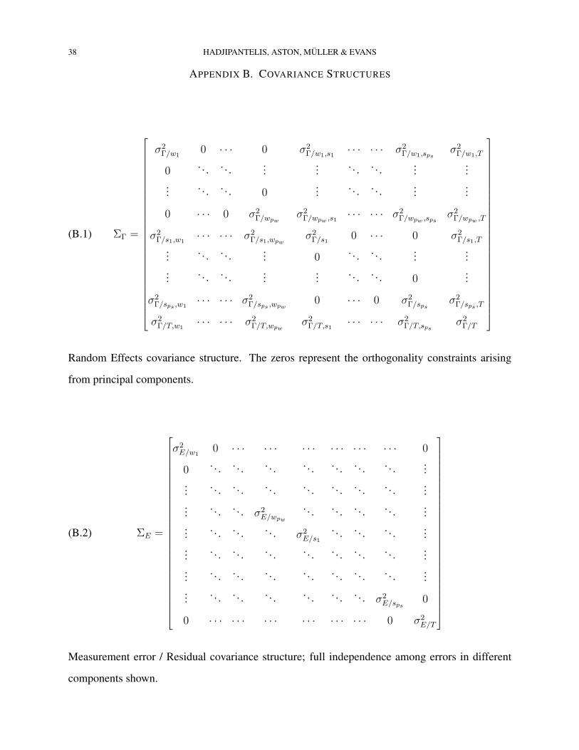
38 HADJIPANTELIS, ASTON, MULLER & EVANS
APPENDIX B. COVARIANCE STRUCTURES
ΣΓ =
σ2Γ/w1
0 · · · 0 σ2Γ/w1,s1
· · · · · · σ2Γ/w1,sps
σ2Γ/w1,T
0 . . . . . . ...... . . . . . . ...
...... . . . . . . 0 ... . . . . . . ...
...
0 · · · 0 σ2Γ/wpw
σ2Γ/wpw ,s1
· · · · · · σ2Γ/wpw ,sps
σ2Γ/wpw ,T
σ2Γ/s1,w1
· · · · · · σ2Γ/s1,wpw
σ2Γ/s1
0 · · · 0 σ2Γ/s1,T
... . . . . . . ... 0 . . . . . . ......
... . . . . . . ...... . . . . . . 0 ...
σ2Γ/sps ,w1
· · · · · · σ2Γ/sps ,wpw
0 · · · 0 σ2Γ/sps
σ2Γ/sps ,T
σ2Γ/T,w1
· · · · · · σ2Γ/T,wpw
σ2Γ/T,s1
· · · · · · σ2Γ/T,sps
σ2Γ/T
(B.1)
Random Effects covariance structure. The zeros represent the orthogonality constraints arising
from principal components.
ΣE =
σ2E/w1
0 · · · · · · · · · · · · · · · · · · 0
0 . . . . . . . . . . . . . . . . . . . . . ...... . . . . . . . . . . . . . . . . . . . . . ...... . . . . . . σ2
E/wpw
. . . . . . . . . . . . ...... . . . . . . . . . σ2
E/s1
. . . . . . . . . ...... . . . . . . . . . . . . . . . . . . . . . ...... . . . . . . . . . . . . . . . . . . . . . ...... . . . . . . . . . . . . . . . . . . σ2
E/sps0
0 · · · · · · · · · · · · · · · · · · 0 σ2E/T
(B.2)
Measurement error / Residual covariance structure; full independence among errors in different
components shown.

UNIFYING AMPLITUDE AND PHASE ANALYSIS 39
APPENDIX C. COMPUTATIONAL ASPECTS OF MULTIVARIATE MIXED EFFECTS REGRESSION
Actual computation of the random effects variances requires a more involved computational ap-
proach than maximizing the restricted log-likelihood given in Eq. (3.23) directly; that is because
in its straightforward form the estimation of det(Ψ) involves the Cholesky decomposition of an
np× np full matrix; a very computationally expensive process both in term of computational time
and memory. Such an approach does not take advantage of the highly structured nature of K and
of the matrices that construct it. To solve this computational issue we use the formulation pre-
sented by Bates and DebRoy [78] for evaluating the profiled REML deviance. This means that we
optimize not for the variance-covariance and measurement error magnitudes directly but of a ratio
between them.
As a result, the vector θ holds ν p(p+1)2 values, ν being the total number of different random effects
structures and p the total number of components in our multivariate MLE; here effectively p = Mw
+ Ms + 1. Starting with the model:
A = XB + ZΓ + E(C.1)
where as beforeA is of dimensionality (n×p),X is of dimensionality (n×k),B is of dimensional-
ity (k×p), Z is of dimensionality (n× l), Γ is of dimensionality (l×p) and E is of dimensionality
(n× p). We decompose it to account for two totally independent random effects as:
A = XB + Z1Γ1 + Z2Γ2 + E(C.2)
where one can assume Z = [Z1Z2] and Γ =[
Γ1Γ2
]based on our assumption of independence
between the two random effects (Speaker and Sentence). Since Z1,Z2,Γ1, Γ2 are of dimensions
(n× l1), (n× l2),(l1 × p) and (l2 × n) respectively, Eq.(C.2) translates in vector notation as:
−→A = (Ip ⊗X)−→B + (Ip ⊗ Z1)−→Γ 1 + (Ip ⊗ Z2)−→Γ 2 +−→E(C.3)

40 HADJIPANTELIS, ASTON, MULLER & EVANS
where we have that :
−→E ∼ N(0,ΣE ⊗ In×n), −→Γ1 ∼ N(0,ΣR1 ⊗ Il1) −→Γ2 ∼ N(0,ΣR2 ⊗ Il2)(C.4)
where ΣE , ΣR1 and ΣR2 are of dimensions (p × p). l1 and l2 being the number of levels in the
Speaker (5) and the Sentence (598) random effects. Significantly ΣR1 and ΣR2 have the same
structure as the matrix in Eq. (B.1). This structure is enforced by multiplying the candidate ΣRi
by a 0 − 1 “boolean matrix” Mi of dimensions (p × p) that sets to zero all entries not explicitly
assumed to be non-zeros by design; effectively updating Ri as:
ΣRi= ΣRi
Mi(C.5)
where is the Hadamard product (or Schur product) between two matrices. Then given that ΣRi
remains a valid covariance matrix, thus being positive definite, it can be expressed as ΣRi= LiL
Ti
and additionally can be expressed in term of a relative precision factor [79] as:
ΣRi
1σ2
= ∆i∆Ti(C.6)
Here σ2 expresses is a “sample-wide” variance that does not reflect any single variance of the p
dimensions of the model. We can use it nevertheless because of our hypothesis that ΣE is diagonal,
therefore the ratio expressed in ∆i can be formulated even it is only for algorithmic simplicity. As
such, going to back to Eq. (C.3) we can re-write it as:
−→A = (Ip ⊗X)−→B + [[(Ip ⊗ Z1)][(Ip ⊗ Z2)]]
[−→Γ 1−→Γ 2
]+−→E(C.7)
and restate the universal random effects (p(l1 + l2)× p(l1 + l2)) matrix ΣRUas:
Σ−1RU
= SST =
S1 0
0 S2
S1 0
0 S2
T
(C.8)
where:
S1 = (∆1 ⊗ Il1) and S2 = (∆2 ⊗ Il2)(C.9)
∆1∆T1 = ΣR1
1σ2
and ∆2∆T2 = ΣR2
1σ2
in accordance with the above.(C.10)

UNIFYING AMPLITUDE AND PHASE ANALYSIS 41
We therefore can reformulate our model as the minimization of following penalized least squares
expression:
minΓ,B
−→A aug − Φ(θ)
−→Γ aug
−→B
(C.11)
where:
Aaug =[A
0
],−→Γ aug =
[−→Γ 1−→Γ 2
], Φ(θ) =
Zaug Xaug
S(θ) 0
,(C.12)
Zaug = [[(Ip ⊗ Z1)][(Ip ⊗ Z2)]] and Xaug = (Ip ⊗X)(C.13)
Aaug being the original n × p matrix A augmented by a zero l × p bottom submatrix leading to a
final dimensionality of (n+ l)×p and Φ(θ) being the augmented model matrix (now of dimensions
p(n + l) × p(k + l)). To solve this we form, proceeding analogously to Bates [78], Φe = [Φ, A]
(of dimensionality p(n + l) × p(l + k + p)) and define RTe Re to be the Cholesky decomposition
of the ΦTe Φe. Thus instead of working with a (np × np) matrix, we now work with a matrix of
dimensions (p(l + k + p)× p(l + k + p)). In particular, in matrix notion we have the following:
ΦTe Φe =
ZTaug S(θ)T
XTaug 0
ATaug 0
Zaug Xaug
−→A aug
S(θ) 0 0
(C.14)
=
ZTaugZaug + Σ−1
RUZTaugXaug ZT
aug
−→A aug
XTaugZaug XT
augXaug XTaug
−→A aug
−→A TaugZaug
−→A TaugXaug
−→A Taug
−→A aug
(C.15)
= RTe Re, where RT
e :
RTe =
RZZ RZX rZA
0 RXX rXA
0 0 rAA
(C.16)
where RZZ and RXX are both upper triangular, non-singular matrices of dimensions pl × pl and
pk × pk respectively; RZX is of dimensionality pl × pk. Similarly, rZA, rXA and rAA are of

42 HADJIPANTELIS, ASTON, MULLER & EVANS
dimensions pl× 1, pk × 1 and 1× 1. As a result the conditional REML estimates for−→B are given
by the solving the following triangular system:
RXX
−→B = rXA(C.17)
Similarly, we have:
σ2 = rTAArAAp(n− k)(C.18)
with the profiled log-restricted-likelihood being:
−2LREML(θ) = log( |ΦTΦ||Σ−1
RU|) + (p(n− k))[1 + log(2πσ2)](C.19)
or the profiled log-likelihood as : − 2LML(θ) = log(|ΦTΦ|) + pn[1 + log(2πrTAArAApn
)](C.20)
Finally, the conditional expected value of Γ is given by the solution of the system:
RZZ
−→Γ aug = rZA −RZX
−→B(C.21)
and the conditional σi, i = 1, . . . , p for a given component of the original multivariate model
equals:
σi =√
1n− k
Σ[(Ai − Ai)2 + U2i ](C.22)
where Ui is the l dimensional random vector such that A = Xaug
−→B + ZaugΣRU
−→U [80].
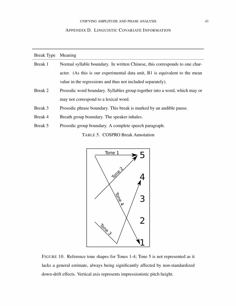
UNIFYING AMPLITUDE AND PHASE ANALYSIS 43
APPENDIX D. LINGUISTIC COVARIATE INFORMATION
Break Type Meaning
Break 1 Normal syllable boundary. In written Chinese, this corresponds to one char-
acter. (As this is our experimental data unit, B1 is equivalent to the mean
value in the regressions and thus not included separately).
Break 2 Prosodic word boundary. Syllables group together into a word, which may or
may not correspond to a lexical word.
Break 3 Prosodic phrase boundary. This break is marked by an audible pause.
Break 4 Breath group boundary. The speaker inhales.
Break 5 Prosodic group boundary. A complete speech paragraph.
TABLE 5. COSPRO Break Annotation
FIGURE 10. Reference tone shapes for Tones 1-4; Tone 5 is not represented as it
lacks a general estimate, always being significantly affected by non-standardized
down-drift effects. Vertical axis represents impressionistic pitch height.
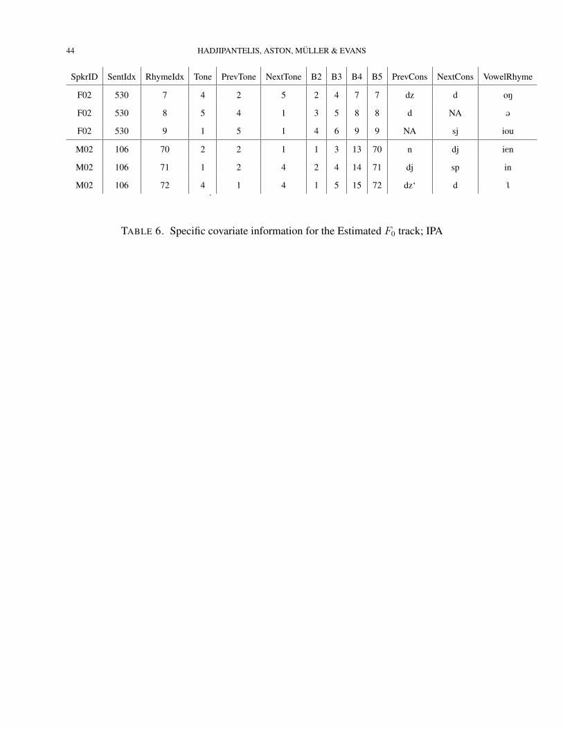
44 HADJIPANTELIS, ASTON, MULLER & EVANS
SpkrID SentIdx RhymeIdx Tone PrevTone NextTone B2 B3 B4 B5 PrevCons NextCons VowelRhyme
F02 530 7 4 2 5 2 4 7 7 dz d oN
F02 530 8 5 4 1 3 5 8 8 d NA @
F02 530 9 1 5 1 4 6 9 9 NA sj iou
M02 106 70 2 2 1 1 3 13 70 n dj ien
M02 106 71 1 2 4 2 4 14 71 dj sp in
M02 106 72 4 1 4 1 5 15 72 dz‘ d ğ.
TABLE 6. Specific covariate information for the Estimated F0 track; IPA

UNIFYING AMPLITUDE AND PHASE ANALYSIS 45
APPENDIX E. NUMERICAL VALUES OF RANDOM EFFECTS CORRELATION MATRICES FOR
AMPLITUDE & PHASE MODEL
PSpkr ID =
1.00 0.00 0.00 0.00 −0.29 −0.09 0.05 0.08 −0.15
0.00 1.00 0.00 0.00 −0.36 0.03 0.03 0.00 −0.89
0.00 0.00 1.00 0.00 0.01 0.04 −0.03 −0.04 −0.04
0.00 0.00 0.00 1.00 −0.03 −0.01 0.00 0.01 0.00
−0.29 −0.36 0.01 −0.03 1.00 0.00 0.00 0.00 0.36
−0.09 0.03 0.04 −0.01 0.00 1.00 0.00 0.00 −0.01
0.05 0.03 −0.03 0.00 0.00 0.00 1.00 0.00 −0.04
0.08 0.00 −0.04 0.01 0.00 0.00 0.00 1.00 −0.01
−0.15 −0.89 −0.04 0.00 0.36 −0.01 −0.04 −0.01 1.00
(E.1)
PSentence =
1.00 0.00 0.00 0.00 −0.89 −0.22 −0.17 0.06 0.42
0.00 1.00 0.00 0.00 0.41 −0.55 −0.09 0.10 0.57
0.00 0.00 1.00 0.00 0.01 −0.27 −0.06 0.85 0.39
0.00 0.00 0.00 1.00 −0.12 −0.39 0.82 −0.03 0.30
−0.89 0.41 0.01 −0.12 1.00 0.00 0.00 0.00 −0.12
−0.22 −0.55 −0.27 −0.39 0.00 1.00 0.00 0.00 −0.51
−0.17 −0.09 −0.06 0.82 0.00 0.00 1.00 0.00 0.14
0.06 0.10 0.85 −0.03 0.00 0.00 0.00 1.00 0.42
0.42 0.57 0.39 0.30 −0.12 −0.51 0.14 0.42 1.00
(E.2)

46 HADJIPANTELIS, ASTON, MULLER & EVANS
APPENDIX F. AREA UNDER THE CURVE - FPCA / MVLME ANALYSIS
To verify the generality of the presented framework the core of the analysis in Sect. 3 was re-
implemented utilizing the Area Under the Curve framework of Zhang & Muller [44]. The results
confirm our assertion that the choice of time-registration framework, while crucial, do not imply
that the findings from a joint analysis, such as the one described in the main body of this work,
are specific to a single framework. The insights offered by the application of FPCA in the new
amplitude and phase variation functions HAUC and SAUC (Figures 11 and 12 respectively) as well
as the insights from the subsequent MVLME analysis of AUC based projections scores (Fig. 13)
communicate very similar insights to the ones as the ones obtained from the approach described in
Sec 4.2.
0 0.1 0.2 0.3 0.4 0.5 0.6 0.7 0.8 0.9 1100
150
200
250
300
350
Hz
T
w Mean response
µw
(u)
0 0.1 0.2 0.3 0.4 0.5 0.6 0.7 0.8 0.9 1−0.6
−0.5
−0.4
−0.3
−0.2
−0.1
0
0.1
0.2
0.3
0.4
0.5
0.6
T
wFPC1 Perc. Var. : 0.8881
wFPC1
0 0.1 0.2 0.3 0.4 0.5 0.6 0.7 0.8 0.9 1−0.6
−0.5
−0.4
−0.3
−0.2
−0.1
0
0.1
0.2
0.3
0.4
0.5
0.6
T
wFPC2 Perc. Var. : 0.0953
wFPC2
0 0.1 0.2 0.3 0.4 0.5 0.6 0.7 0.8 0.9 1−0.6
−0.5
−0.4
−0.3
−0.2
−0.1
0
0.1
0.2
0.3
0.4
0.5
0.6
T
wFPC3 Perc. Var. : 0.0122
wFPC3
0 0.1 0.2 0.3 0.4 0.5 0.6 0.7 0.8 0.9 1−0.6
−0.5
−0.4
−0.3
−0.2
−0.1
0
0.1
0.2
0.3
0.4
0.5
0.6
T
wFPC4 Perc. Var. : 0.0027
wFPC4
0 0.1 0.2 0.3 0.4 0.5 0.6 0.7 0.8 0.9 1−0.6
−0.5
−0.4
−0.3
−0.2
−0.1
0
0.1
0.2
0.3
0.4
0.5
0.6
T
wFPC5 & 6 Perc. Var. : 0.0009, 0.0004
wFPC5
wFPC6
FIGURE 11. WAUC (Amplitude) Functional Principal Components ΦAUC com-
puted when using an AUC time-registration framework: Mean function ([.05,.95]
percentiles shown in grey) and 1st, 2nd, 3rd, 4th, 5th, and 6th functional principal
components of amplitude.
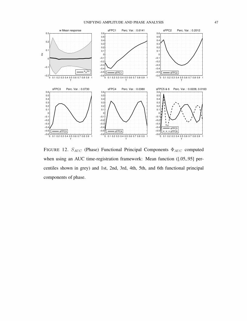
UNIFYING AMPLITUDE AND PHASE ANALYSIS 47
0 0.1 0.2 0.3 0.4 0.5 0.6 0.7 0.8 0.9 1−0.2
−0.1
0
0.1
0.2
0.3
Hz
T
w Mean response
µw
(u)
0 0.1 0.2 0.3 0.4 0.5 0.6 0.7 0.8 0.9 1−0.6
−0.5
−0.4
−0.3
−0.2
−0.1
0
0.1
0.2
0.3
0.4
0.5
0.6
T
sFPC1 Perc. Var. : 0.6141
sFPC1
0 0.1 0.2 0.3 0.4 0.5 0.6 0.7 0.8 0.9 1−0.6
−0.5
−0.4
−0.3
−0.2
−0.1
0
0.1
0.2
0.3
0.4
0.5
0.6
T
sFPC2 Perc. Var. : 0.2012
sFPC2
0 0.1 0.2 0.3 0.4 0.5 0.6 0.7 0.8 0.9 1−0.6
−0.5
−0.4
−0.3
−0.2
−0.1
0
0.1
0.2
0.3
0.4
0.5
0.6
T
sFPC3 Perc. Var. : 0.0730
sFPC3
0 0.1 0.2 0.3 0.4 0.5 0.6 0.7 0.8 0.9 1−0.6
−0.5
−0.4
−0.3
−0.2
−0.1
0
0.1
0.2
0.3
0.4
0.5
0.6
T
sFPC4 Perc. Var. : 0.0380
sFPC4
0 0.1 0.2 0.3 0.4 0.5 0.6 0.7 0.8 0.9 1−0.6
−0.5
−0.4
−0.3
−0.2
−0.1
0
0.1
0.2
0.3
0.4
0.5
0.6
T
sFPC5 & 6 Perc. Var. : 0.0228, 0.0163
sFPC5
sFPC6
FIGURE 12. SAUC (Phase) Functional Principal Components ΦAUC computed
when using an AUC time-registration framework: Mean function ([.05,.95] per-
centiles shown in grey) and 1st, 2nd, 3rd, 4th, 5th, and 6th functional principal
components of phase.
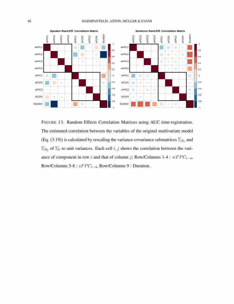
48 HADJIPANTELIS, ASTON, MULLER & EVANS
−1
−0.8
−0.6
−0.4
−0.2
0
0.2
0.4
0.6
0.8
1
wF
PC
1
wF
PC
2
wF
PC
3
wF
PC
4
sFP
C1
sFC
P2
sFP
C3
sFC
P4
Dur
atio
n
wFPC1
wFPC2
wFPC3
wFPC4
sFPC1
sFCP2
sFPC3
sFCP4
Duration
Speaker Rand.Eff. Correlation Matrix
−1
−0.8
−0.6
−0.4
−0.2
0
0.2
0.4
0.6
0.8
1
wF
PC
1
wF
PC
2
wF
PC
3
wF
PC
4
sFP
C1
sFC
P2
sFP
C3
sFC
P4
Dur
atio
n
wFPC1
wFPC2
wFPC3
wFPC4
sFPC1
sFCP2
sFPC3
sFCP4
Duration
Sentence Rand.Eff. Correlation Matrix
FIGURE 13. Random Effects Correlation Matrices using AUC time-registration.
The estimated correlation between the variables of the original multivariate model
(Eq. (3.19)) is calculated by rescaling the variance-covariance submatrices ΣR1 and
ΣR2 of ΣΓ to unit variances. Each cell i, j shows the correlation between the vari-
ance of component in row i and that of column j; Row/Columns 1-4 : wFPC1−4,
Row/Columns 5-8 : sFPC1−4, Row/Columns 9 : Duration.

UNIFYING AMPLITUDE AND PHASE ANALYSIS 49
ADDRESS FOR CORRESPONDENCE:
JOHN ASTON
STATISTICAL LABORATORY
DEPARTMENT OF PURE MATHS AND MATHEMATICAL STATISTICS
UNIVERSITY OF CAMBRIDGE TEL: +44-1223-766535
CAMBRIDGE EMAIL: [email protected]
UK


![(Non)existence of Pleated Folds: How Paper Folds …0906.4747v1 [cs.CG] 25 Jun 2009 (Non)existence of Pleated Folds: How Paper Folds Between Creases Erik D. Demaine∗† Martin L.](https://static.fdocuments.us/doc/165x107/5aee331f7f8b9ae5319163fc/nonexistence-of-pleated-folds-how-paper-folds-09064747v1-cscg-25-jun.jpg)