Unified Inference for Sparse and Dense Longitudinal Data in...
17
Scandinavian Journal of Statistics, Vol. 44: 268–284, 2017 doi: 10.1111/sjos.12253 © 2016 Board of the Foundation of the Scandinavian Journal of Statistics. Published by Wiley Publishing Ltd. Unified Inference for Sparse and Dense Longitudinal Data in Time-varying Coefficient Models YIXIN CHEN Department of Biostatistics and Programming, Sanofi Genzyme WEIXIN YAO Department of Statistics, University of California, Riverside ABSTRACT. Time-varying coefficient models are widely used in longitudinal data analysis. These models allow the effects of predictors on response to vary over time. In this article, we consider a mixed-effects time-varying coefficient model to account for the within subject correlation for longitudinal data. We show that when kernel smoothing is used to estimate the smooth functions in time-varying coefficient models for sparse or dense longitudinal data, the asymptotic results of these two situations are essentially different. Therefore, a subjective choice between the sparse and dense cases might lead to erroneous conclusions for statistical inference. In order to solve this problem, we establish a unified self-normalized central limit theorem, based on which a unified inference is proposed without deciding whether the data are sparse or dense. The effectiveness of the proposed unified inference is demonstrated through a simulation study and an analysis of Baltimore MACS data. Key words: kernel smoothing, longitudinal data, self-normalization, time-varying coefficient models 1. Introduction Longitudinal data sets arise in biostatistics and lifetime testing problems when the responses of the individuals are recorded repeatedly over a period of time. Examples can be found in clinical trials, follow-up studies for monitoring disease progression, and observational cohort studies. In many longitudinal studies, repeated measurements of the response variable are collected at irregular and possibly subject-specific time points. Therefore, the measurements within each subject are possibly correlated with each other, and data are often highly unbalanced, but dif- ferent subjects can be assumed to be independent. Typically, the scientific interest is either in the pattern of change over time of the outcome measures or more simply in the dependence of the outcome on the covariates. A useful nonparametric model to quantify the influence of covariates other than time is the time-varying coefficient model, in which coefficients are allowed to change smoothly over time. Let ¹.y ij ; x i .t ij /;t ij /I i D 1;2;:::;nI j D 1;2;:::;n i º be a longitudinal sample from n randomly selected subjects, where t ij is the time when the j th measurement of the i th subject is made and assumed to have bounded support, n i is the number of repeated measurements of the i th subject, y ij is the response and x i .t ij / D x ij D x 0 i ;x 1 i .t ij /;:::;x k i .t ij / T are the .k C 1/-dimensional covariates for the i th subject at time t ij , where x 0 i D 1 is an optional intercept. The total number of observations in this sample is N D P n i D1 n i . The time-varying coefficient model can be written as y ij D x T ij ˇ.t ij / C i .t ij /; (1.1) where ˇ.t/ D .ˇ 0 .t/;ˇ 1 .t/;:::;ˇ k .t// T for all t 0 are smooth functions of t , i .t/ is a realization of a zero-mean stochastic process .t/, and x ij and i are independent.
-
Upload
nguyenphuc -
Category
Documents
-
view
221 -
download
0
Transcript of Unified Inference for Sparse and Dense Longitudinal Data in...
Scandinavian Journal of Statistics, Vol. 44: 268 –284, 2017
doi: 10.1111/sjos.12253© 2016 Board of the Foundation of the Scandinavian Journal of Statistics. Published by Wiley Publishing Ltd.
Unified Inference for Sparse and DenseLongitudinal Data in Time-varyingCoefficient ModelsYIXIN CHENDepartment of Biostatistics and Programming, Sanofi Genzyme
WEIXIN YAODepartment of Statistics, University of California, Riverside
ABSTRACT. Time-varying coefficient models are widely used in longitudinal data analysis. Thesemodels allow the effects of predictors on response to vary over time. In this article, we considera mixed-effects time-varying coefficient model to account for the within subject correlation forlongitudinal data. We show that when kernel smoothing is used to estimate the smooth functionsin time-varying coefficient models for sparse or dense longitudinal data, the asymptotic resultsof these two situations are essentially different. Therefore, a subjective choice between the sparseand dense cases might lead to erroneous conclusions for statistical inference. In order to solve thisproblem, we establish a unified self-normalized central limit theorem, based on which a unifiedinference is proposed without deciding whether the data are sparse or dense. The effectiveness of theproposed unified inference is demonstrated through a simulation study and an analysis of BaltimoreMACS data.
Key words: kernel smoothing, longitudinal data, self-normalization, time-varying coefficientmodels
1. Introduction
Longitudinal data sets arise in biostatistics and lifetime testing problems when the responses ofthe individuals are recorded repeatedly over a period of time. Examples can be found in clinicaltrials, follow-up studies for monitoring disease progression, and observational cohort studies.In many longitudinal studies, repeated measurements of the response variable are collected atirregular and possibly subject-specific time points. Therefore, the measurements within eachsubject are possibly correlated with each other, and data are often highly unbalanced, but dif-ferent subjects can be assumed to be independent. Typically, the scientific interest is either inthe pattern of change over time of the outcome measures or more simply in the dependence ofthe outcome on the covariates.
A useful nonparametric model to quantify the influence of covariates other than time isthe time-varying coefficient model, in which coefficients are allowed to change smoothly overtime. Let ¹.yij ; xi .tij /; tij /I i D 1; 2; : : : ; nI j D 1; 2; : : : ; ni º be a longitudinal sample from n
randomly selected subjects, where tij is the time when the j th measurement of the i th subjectis made and assumed to have bounded support, ni is the number of repeated measurements
of the i th subject, yij is the response and xi .tij / D xij D�x0i; x1i.tij /; : : : ; x
ki.tij /
�Tare the
.k C 1/-dimensional covariates for the i th subject at time tij , where x0iD 1 is an optional
intercept. The total number of observations in this sample is N DPniD1 ni . The time-varying
coefficient model can be written as
yij D xTijˇ.tij /C �i .tij /; (1.1)
where ˇ.t/ D .ˇ0.t/; ˇ1.t/; : : : ; ˇk.t//T for all t � 0 are smooth functions of t , �i .t/ is a
realization of a zero-mean stochastic process �.t/, and xij and �i are independent.
Scand J Statist 44 Time-varying coefficient models 269
To better account for the local correlation structure of the longitudinal data, similar to thenonparametric mixed-effects model used by Wu & Zhang (2002) and Kim & Zhao (2013),we add a subject-specific random trajectory vi .�/ to model (1.1) and consider the followingmixed-effects time-varying coefficient model
yij D xTijˇ.tij /C vi .tij /C �.tij /�ij ; (1.2)
where vi .t/ is a realization of a mean 0 process with a covariance function �.t; t0/ D
cov°vi .t/; vi .t
0/±D EŒvi .t/vi .t
0/�, �ij are errors with E.�ij / D 0 and E.�2
ij/ D 1, and vi .t/
and �ij are assumed to be independent. Model (1.2) is basically the same as the model ofHoover et al. (1998) and is a special case of the model investigated by Liang et al. (2003) andTian & Wu (2014), which also includes subject-specific coefficients. Our primary goal in thisarticle is to estimate the varying coefficients ˇ.t/ and construct confidence intervals for them.
Longitudinal data can be identified as sparse or dense according to the number of measure-ments within each subject. Statistical analyses for sparse or dense longitudinal data have been asubject of intense investigation in the recent ten years. Please see, for example, Yao et al. (2005)and Ma et al. (2012) for the studies of the sparse longitudinal data when ni is assumed to bebounded or follows a given distribution with E.ni / <1; see, for example, Fan & Zhang (2000)and Zhang & Chen (2007) for the studies of the dense longitudinal data when ni !1. Kim &Zhao (2013) specified the sparse and dense cases clearly. Here, we adopt their assumptions forthe number of repeated measurements of each subject under these two scenarios:
� Sparse longitudinal data: n1; n2; : : : ; nn are independent and identically distributedpositive-integer-valued random variables with E.ni / <1;
� Dense longitudinal data: min1�i�n.ni / �Mn for some Mn !1 as n!1.
Other assumptions regarding the number of repeated measurements within each subject werealso used to study asymptotic behaviours of local polynomial estimators in varying coefficientmodels. These assumptions are more or less similar to sparse or dense longitudinal data def-initions described earlier. For example, in Hoover et al. (1998) and Wu & Chiang (2000), theasymptotic inference was established under the assumption of max1�i�n.niN�1/ ! 0 asn!1. This assumption covers the sparse longitudinal data condition defined earlier but doesnot meet the definition of dense longitudinal data. In practice, it is well known that the bound-ary between sparse and dense cases is not always clear. A subjective choice between sparse anddense cases may pose challenges for statistical inference. Furthermore, asymptotic propertiesof estimators could be different under sparse and dense assumptions. For example, as pointedout in Wu & Chiang (2000), estimators proposed in Hoover et al. (1998) may not be consis-tent under the dense data setting. Li & Hsing (2010) established a uniform convergence ratefor weighted local linear estimation of mean and variance functions for functional/longitudinaldata. Nevertheless, Kim & Zhao (2013) showed that convergence rates and limiting variancesunder sparse and dense assumptions are different. This motivated them to develop unifiednonparametric approaches to perform longitudinal data analysis without deciding whether thedata are dense or sparse. However, Kim & Zhao (2013) only considered estimating the meanresponse curve without the presence of covariates.
In this article, we use the mixed-effects time-varying coefficient model (1.2) to take covariatesother than time into account. The time-varying coefficient part, ˇ.t/, in this model describesthe effect of interest. The model considered by Kim & Zhao (2013) is a special case of ours ifxij=1. We first show that when using kernel smoothing to estimate smooth functions for sparseor dense longitudinal data, asymptotic results of these two situations are essentially different.
© 2016 Board of the Foundation of the Scandinavian Journal of Statistics.
270 Y. Chen and W. Yao Scand J Statist 44
Therefore, a subjective choice between sparse and dense cases could lead to wrong conclusionsfor statistical inference. In order to solve this problem, motivated by Kim & Zhao (2013), weestablish a unified self-normalized central limit theorem, based on which a unified inferenceis proposed that can adapt to both sparse and dense cases. The resulting unified confidenceinterval is simple to compute and use in practice. The effectiveness of the proposed unifiedinference is demonstrated through a simulation study and an analysis of Baltimore MACS data.
This article is organized as follows. In section 2, we first introduce a sample size weightedlocal constant estimator of the smooth functions ˇ.t/ and provide asymptotic properties forboth sparse and dense longitudinal data. Under the mixed-effects time-varying coefficientmodel setting, we then propose a unified convergence theory based on a self-normalizationtechnique. In section 3, we provide numerical results from a simulation study and use the Balti-more MACS data to demonstrate the performance of the proposed unified approach. Section 4contains some discussion. Regularity conditions and proofs are assembled in the Appendix.
2. A unified approach for longitudinal data
2.1. Estimation method
Hoover et al. (1998) proposed a local constant fit for the time-varying coefficient model. How-ever, they did not consider the effect of repeated measurements for each subject. Similar to Li& Hsing (2010), we consider a sample size weighted local constant estimation method for themodel (1.2). Let f .�/ be the density function of tij and let t be an interior point of the supportof f .�/. The weighted local constant estimator we consider is
O .t/ D arg minˇ
nXiD1
1
ni
niXjD1
hyij � xTijˇ.t/
i2K
�tij � t
hn
�D H�1n gn; (2.1)
where K.�/ is a kernel function that is symmetric about 0 and satisfiesRRK.u/ du D 1 and
hn > 0 is a bandwidth, depending on n, with
Hn DnXiD1
1
ni
niXjD1
xijxTijK�tij � t
hn
�; gn D
nXiD1
1
ni
niXjD1
xijyijK�tij � t
hn
�: (2.2)
Similar to the estimator considered by Kim & Zhao (2013), the just shown estimator doesnot take within-subject correlations into account for the simplicity of explanation. How-ever, the statistical inference we establish in this article takes within-subject correlations intoaccount and is based on the model assumption (1.2). Based on Lin & Carroll (2000), the work-ing independence kernel regression estimate O .t/ of (2.1) is still consistent and can achieveoptimal convergence rate. However, the working independence estimate might lose some effi-ciency compared with many proposed methods that incorporate within-subject correlationsinto nonparametric regression estimator. See, for example, Fan et al. (2007), Fan & Wu (2008),Pourahmadi (2007), Pan & Mackenzie (2003), Ye & Pan (2006), Zhang & Leng (2012), Yao &Li (2013) and Zhang et al. (2015).
2.2. Asymptotic properties for sparse and dense longitudinal data
Based on sparse and dense cases specified in Kim & Zhao (2013), we will show that convergencerates and limiting variances of O .t/ are different for sparse and dense longitudinal data. To gainintuition about this, we decompose the difference between the estimated value O .t/ and the truevalue ˇ.t/ in the following way:
© 2016 Board of the Foundation of the Scandinavian Journal of Statistics.

Scand J Statist 44 Time-varying coefficient models 271
O .t/ � ˇ.t/ �H�1n
nXiD1
1
ni
niXjD1
xijhxTijˇ.tij / � xTijˇ.t/
iK
�tij � t
hn
�D H�1n
nXiD1
�i ;
(2.3)
where the asymptotic distribution of O .t/ is determined by the right-hand side, with
�i D1
ni
niXjD1
�ij ; �ij D xij�vi .tij /C �.tij /�ij
�K
�tij � t
hn
�: (2.4)
Based on the previous definition �.t; t0/ D cov
°vi .t/; vi .t
0/±D E
hvi .t/vi .t
0/i
and
E��ij �
T
ij0
D E
°E��ij �
T
ij0 j tij ; tij 0
±, we have, for j ¤ j
0,
E��ij �
T
ij0
DE
²G.tij ; tij 0 /�.tij ; tij 0 /K
�tij � t
hn
�K
�tij 0 � t
hn
�³� h2nG.t; t/f 2.t/�.t; t/;
(2.5)
where G.tij ; tij 0 / D E�
xijxTij0 j tij ; tij 0
and G.t; t/ D lim
t0!t
G.t; t0/. Throughout this article,
an � bn means that an=bn ! 1. For the same subject and same time point,
E��ij �
Tij
D E
²�.tij /
h�.tij ; tij /C �
2.tij /iK2
�tij � t
hn
�³
� �.t/hnf .t/ k
h�.t; t/C �2.t/
i;
(2.6)
where �.tij / D E�
xijxTijjtij
and K D
RRK2.u/ du. Because
var.�i jni / D n�2i
8<:niXjD1
E��ij �
Tij
C
X1�j¤j
0�ni
E��ij �
T
ij0
9=; ;
then by (2.5) and (2.6), we have the following result:
var.�i jni / �1
ni�.t/hnf .t/ K
h�.t; t/C �2.t/
iC
�1 �
1
ni
�G.t; t/h2nf
2.t/�.t; t/: (2.7)
Under the sparse assumption that ni ’s are independent and identically distributed withE.ni / < 1, we have, var.�i jni / � �.t/hnf .t/ K
��.t; t/C �2.t/
�=ni as hn ! 0; under
the dense assumption that min1�i�n.ni / � Mn for some Mn ! 1 as n ! 1, wehave var.�i jni / � G.t; t/h2nf
2.t/�.t; t/ with Mnhn ! 1. Therefore, limiting variances forsparse and dense cases are substantially different. We state asymptotic properties for these twoscenarios in the following theorem.
Theorem 2.1. Let
�.t/ D
"ˇ0
.t/f0.t/
f .t/Cˇ00
.t/
2C ��1.t/�
0
.t/ˇ0
.t/
#ZR
u2K.u/ du:
© 2016 Board of the Foundation of the Scandinavian Journal of Statistics.

272 Y. Chen and W. Yao Scand J Statist 44
Based on the regularity conditions in the Appendix, we have the following asymptotic results.
� Sparse data: Assume nhn !1 and supnnh5n <1. Then
pnhn
hO .t/ � ˇ.t/ � h2n�.t/
i! N
�0kC1;†sparse.t/
�; (2.8)
where †sparse.t/ D ��1.t/ K
��.t; t/C �2.t/
��=f .t/, 0kC1 is a .k C 1/ � 1 vector with
each entry being 0, and � D E.1=n1/.� Dense data: Assume �.t; t/ ¤ 0, ni � Mn, Mnhn ! 1, nhn ! 1 and supnnh4n < 1.
Then
pnhO .t/ � ˇ.t/ � h2n�.t/
i! N .0kC1;†dense.t// ; (2.9)
where †dense.t/ D ��1.t/G.t; t/�.t; t/��1.t/.
Based on Theorem 2.1, O .t/ has the traditional nonparametric convergence rate if the dataare sparse, but has root n convergence rate if the data are dense. In addition, note that, if x D 1,then Theorem 2.1 simplifies to asymptotic results provided by Kim & Zhao (2013). Based onthe asymptotic normality in Theorem 2.1, confidence intervals for ˇ.t/ are different undersparse and dense assumptions. Let ´1�˛=2 be the 1 � ˛=2 standard normal quantile. Then anasymptotic 1 � ˛ confidence interval for the smooth function ˇl .t/, l D 0; : : : ; k is
Ol .t/�h
2n O�l .t/˙´1�˛=2.nhn/
�1=2
²hO��1.t/ K
hO�.t; t/C O�2.t/
iO�= Of .t/
i1=2³l;l
(2.10)
for sparse data or
Ol .t/ � h
2n O�l .t/˙ ´1�˛=2n
�1=2
²hO��1.t/ OG.t; t/ O�.t; t/ O�
�1.t/i1=2³
l;l
(2.11)
for dense data, where ˇ.t/ D .ˇ0.t/; ˇ1.t/; : : : ; ˇk.t//T , Ol .t/ is the .l C 1/th element of
O .t/, O�l .t/ is the .l C 1/th element of O�.t/ and the subscript .l; l/ refers to the .l C 1/thdiagonal element of a matrix. In the aforementioned formulas, O� D n�1
PniD1 n
�1i
, O�.t; t/,
O�2.t/, Of .t/, O�l .t/, O��1.t/, and OG.t; t/ are consistent estimates of � , �.t; t/, �2.t/, f .t/, �l .t/,
��1.t/ and G.t; t/. In practice, f .t/ can be estimated by kernel density estimate, Of .t/ DN�1
PniD1
PnijD1
Khn.tij � t /, whereKhn.t/ D h�1n K.t=hn/. The nonparametric mean func-
tions �.t/, �.t; t 0/ and G.t; t 0/ can be estimated by kernel smoothing methods. For example,O�lm.t/ D N�1
PniD1
PnijD1
xijlxijmKhn.tij � t /, where �lm.t/ is the .l; m/th element of�.t/ and xijl is the lth element of xij . Then �.t/ and �.t/ can be easily estimated by notingthat var¹y.tij /º D �2.tij /C �.tij ; tij /.
2.3. Proposed unified approach
From Section 2.2, asymptotic results for sparse and dense longitudinal data are essentially dif-ferent, and thus, a subjective choice between these two situations poses challenges for statisticalinference, which motivates us to find a unified approach. In this section, we propose a uni-fied self-normalized central limit theorem that can adapt to both sparse and dense cases forthe mixed-effects time-varying coefficient model (1.2). Let Un.t/ D H�1n WnH�1n ; where Hn isdefined in (2.2), and
© 2016 Board of the Foundation of the Scandinavian Journal of Statistics.
Scand J Statist 44 Time-varying coefficient models 273
Wn D
nXiD1
8<: 1
ni
niXjD1
xijhyij � xTij O .tij /
iK
�tij � t
hn
�9=;
�
8<: 1
ni
niXjD1
xTijhyij � xTij O .tij /
iK
�tij � t
hn
�9=; :
We have the following unified central limit theorem.
Theorem 2.2. Assume nhn= logn ! 1 and supn nh5n < 1 for sparse data or ni � Mn,
Mnhn ! 1, nh2n= logn ! 1 and supn nh4n < 1 for dense data. Under the regularity
conditions in the Appendix,
U n.t/�1=2
hO .t/ � ˇ.t/ � h2n�.t/
i! N.0kC1; IkC1/
in both sparse and dense settings, where IkC1 is the .k C 1/ � .k C 1/ identity matrix.
Note that the central limit theorem proposed in Kim & Zhao (2013) is a special case ofTheorem 2.2 if x D 1 is assumed in model (1.2). Based on Theorem 2.2, a unified asymptoticpointwise 1 � ˛ confidence interval for ˇl .t/, l D 0; : : : ; k can be written as follows:
Ol .t/ � h
2n O�l .t/˙ ´1�˛=2
hUn.t/1=2
il;l: (2.12)
The confidence intervals (2.10) and (2.11) in section 2.2 require estimates of the within-subject covariance function �.t; t/, the overall noise variance function �2.t/ and the condi-tional expectation G.t; t/; which need extra smoothing procedures, but (2.12) does not needsuch estimates and can be used for both sparse and dense cases through the self-normalizerUn.t/1=2.
Because of the bias term h2n�l .t/, it is possible that the estimate Ol .t/ is outside the confi-dence interval. Because it is difficult to estimate the bias h2n�.t/ in practice due to unknownderivatives f
0, ˇ0
, ˇ00
and�0
, we use the same kernel function as in Kim & Zhao (2013),K.u/ D2G.u/ � G.u=
p2/=p2, where G.u/ is the standard normal density. Then
RRu2K.u/ du D 0
and therefore �.t/ D 0kC1. This obviously does not solve the bias problem. For instance, iff , ˇ and � are four times differentiable, then we have the higher order bias term O.h4n/. AsKim & Zhao (2013) stated, the bias problem is an inherently difficult problem and no goodsolutions exist so far. Our simulation results in section 3.1 demonstrate that the new proposedself-normalized confidence interval works well.
For kernel regression, the selection of bandwidth is generally more important than the selec-tion of kernel functions. As stated in Wu & Chiang (2000), under-smoothing or over-smoothingis mainly caused by inappropriate bandwidth choices in practice but is rarely influenced bykernel shapes. The asymptotic optimal bandwidth depends on n and ni , and it should be ableto balance the asymptotic bias term h2n�.t/ and the asymptotic variance term Un.t/. How-ever, as proved in Theorem 2.1, asymptotic properties of the variance term Un.t/ depend onwhether the data are dense or sparse and how ni increases with n. Therefore, it is not easy toderive a unified asymptotic optimal bandwidth. To select the bandwidth for O in practice, weuse the idea of ‘leave-one-subject-out’ cross-validation procedure suggested by Rice & Silver-man (1991). Let O�i .t/ be a kernel estimator of ˇ.t/ computed using the data with all repeatedmeasurements of the i th subject left out and define
© 2016 Board of the Foundation of the Scandinavian Journal of Statistics.

274 Y. Chen and W. Yao Scand J Statist 44
CV.hn/ DnXiD1
1
ni
niXjD1
°yij � xTij O�i .tij /
±2(2.13)
to be the subject-based cross-validation. The optimal bandwidth is then defined to be theunique minimizer of CV.hn/. Based on remark 2.3 of Wu & Chiang (2000), the aforementionedCV bandwidth approximately minimizes the following average squared error:
ASE. O / DnXiD1
1
ni
niXjD1
hxTij
°ˇ.tij / � O .tij /
±i2:
3. Simulation and real data application
3.1. Simulation study
We follow Kim & Zhao (2013) to construct the subject-specific random trajectory vi .�/.Consider the model
yij D
2XlD0
ˇl .tij /xijl .tij /C
3XmD1
˛imˆm.tij /C ��ij ; i D 1; : : : ; nI j D 1; : : : ; ni ;
where ˛im � N.0; !m/ and �ij � N.0; 1/. Let ˇ0.t/ D 5.t � 0:6/2, ˇ1.t/ D cos.3t/,ˇ2.t/ D sin.2t/, ˆ1.t/ D 1, ˆ2.t/ D
p2 sin.2t/, ˆ3.t/ D
p2 cos.2t/, .!1; !2; !3/ D
.0:6; 0:3; 0:1/ and � D 1. Then the variance function �.t; t/ D 0:6 C 0:6 sin2.2t/ C0:2 cos2.2t/. The time points tij are uniformly distributed on Œ0; 1�. To generate covariates, letbi1 � N.0; 0:3/, bi2 � N.0; 0:3/, ij � N.0; 1/, ıij � N.0; 1/ and '.t/ D
p2.t C 1/; then set
xij0 D 1, xij1 D bi1'.tij /Cij and xij2 D bi2'.tij /Cıij for i D 1; : : : ; n and j D 1; : : : ; ni .We consider two sample sizes, n D 200 or 400. Under this setting, we have the following con-
ditional expectations: �.tij / D E�
xijxTijj tij
D diag¹1; 0:6.tij C 1/2 C 1; 0:6.tij C 1/2 C 1º
and
G.tij ; tij / D limtij0!tij
E�
xijxTij 0 j tij ; tij 0D diag¹1; 0:6.tij C 1/
2; 0:6.tij C 1/2º:
For the vector .n1; n2; : : : ; nn/ of the number of repeated measurements on each subject, weconsider four cases
N1 W ni � U Œ¹5; 6; : : : ; 15º�I N2 W ni � U Œ¹15; 16; : : : ; 35º�I (3.1)
N3 W ni � U Œ¹80; 81; : : : ; 120º�I N4 W ni � U Œ¹150; 151; : : : ; 250º�: (3.2)
Here, U ŒD� represents the discrete uniform distribution on a finite set D. Five confidenceintervals are compared in our simulation study:
(1) The self-normalization-based confidence interval in (2.12) (SN);(2) The asymptotic normality-based confidence interval (2.10) for sparse data (NS);(3) The asymptotic normality-based confidence intervals (2.11) for dense data (ND);(4) The bootstrap confidence interval with 200 bootstrap replications from sampling
subjects with replacement (BS);(5) The infeasible confidence interval (NSD)
© 2016 Board of the Foundation of the Scandinavian Journal of Statistics.
Scand J Statist 44 Time-varying coefficient models 275
Ol .t/ � h
2n O�l .t/˙ ´1�˛=2n
�1=2Sl;l ; (3.3)
where S D°��1.t/G.t; t/��1.t/.1 � O�/�.t; t/C ��1.t/ O� K
��.t; t/C �2.t/
�=
Œhnf .t/�º1=2.
The confidence interval NSD is used as a benchmark to compare the performance of theother confidence intervals, because NSD uses the true theoretical limiting variance function(2.7). Note, however, that NSD is practically infeasible, because it depends on many unknownfunctions. Similar to Kim & Zhao (2013), we use the true functions �.t; t/, �2.t/, f .t/, �.t/ andG.t; t/ for NS, ND and NSD, which gives an advantage to these three methods and removesthe impact of different estimation methods. Note that the proposed self-normalization-basedconfidence interval SN only requires a point estimate of ˇ.t/ and thus is very easy to implement.We would like to demonstrate that our new method SN works comparably or better than NSand ND even when true functions are used for NS and ND.
To measure the performance of different confidence intervals, we use the following twocriteria: empirical coverage probabilities and lengths of confidence intervals. Let t1 <
� � � < t20 be 20 grid points evenly spaced on Œ0:1; 0:9�. For each grid point tj .j D
1; : : : ; 20/ and a given confidence level, we construct confidence intervals for smooth func-tions ˇ0.tj /, ˇ1.tj / and ˇ2.tj / and compute the empirical coverage probabilities basedon 500 replications. Using 500 replications is restricted by the computing time basedon a personal computer with Intel(R) Core(TM) i5 CPU, 4-GB installed memory and32-bit operating system. For each of the five confidence intervals, the empirical cover-age probabilities and lengths are averaged at 20 grid points. The bandwidth used foreach replicate is the average of 20 optimal bandwidths in (2.13) based on 20 replications(Kim & Zhao, 2013).
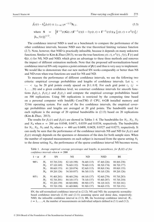
The results for ˇ1.t/ and ˇ2.t/ are showed in Tables 1–4. The bandwidths for N1, N2, N3and N4 when n D 200 are 0.0548, 0.0471, 0.0359 and 0.0334, respectively. The bandwidthsfor N1, N2, N3 and N4 when n D 400 are 0.0498, 0.0428, 0.0327 and 0.0273, respectively. Itcan easily be seen that the performance of the confidence intervals NS and ND for ˇ1.t/ andˇ2.t/ strongly depends on the spareness or denseness of the data for both sample sizes. Whenthe number of repeated measurements on each subject is increased from the sparse setting N1to the dense setting N4, the performance of the sparse confidence interval NS becomes worse,
Table 1. Average empirical coverage percentages and lengths, in parentheses, for ˇ1.t/ of fiveconfidence intervals when n D 200
1� ˛ N SN NS ND NSD BS
90% N1 85.7(0.218) 82.1(0.198) 56.4(0.115) 87.4(0.226) 88.8(0.238)N2 87.1(0.169) 76.6(0.132) 70.4(0.115) 88.5(0.174) 88.7(0.177)N3 88.6(0.133) 61.2(0.074) 82.6(0.115) 89.8(0.136) 89.0(0.135)N4 89.2(0.126) 54.5(0.057) 86.3(0.115) 90.1(0.128) 89.2(0.126)
95% N1 91.4(0.261) 88.4(0.236) 64.1(0.137) 92.6(0.270) 93.7(0.283)N2 92.7(0.201) 84.1(0.157) 78.1(0.137) 93.4(0.207) 93.7(0.210)N3 93.2(0.159) 68.8(0.088) 88.9(0.137) 94.1(0.163) 93.5(0.161)N4 93.7(0.150) 61.4(0.068) 91.9(0.137) 94.6(0.153) 93.7(0.151)
SN, the self-normalized confidence interval in (2.12); NS and ND, the asymptotic normality-based confidence intervals (2.10) and (2.11) assuming sparse and dense data, respectively;NSD, the infeasible confidence interval in (3.3); BS, the bootstrap confidence interval; Ni ,i D 1; : : : ; 4, the number of measurements on individual subjects defined in (3.1) and (3.2).
© 2016 Board of the Foundation of the Scandinavian Journal of Statistics.
276 Y. Chen and W. Yao Scand J Statist 44
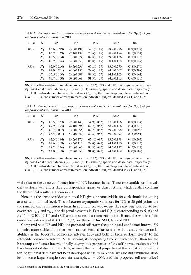
Table 2. Average empirical coverage percentages and lengths, in parentheses, for ˇ2.t/ of fiveconfidence intervals when n D 200
1� ˛ N SN NS ND NSD BS
90% N1 86.6(0.219) 83.0(0.198) 57.1(0.115) 88.2(0.226) 88.9(0.232)N2 86.9(0.169) 77.1(0.132) 70.6(0.115) 88.2(0.174) 88.1(0.174)N3 88.5(0.134) 61.6(0.074) 82.8(0.115) 89.6(0.136) 88.7(0.135)N4 88.9(0.126) 54.0(0.057) 85.8(0.115) 90.1(0.128) 89.0(0.127)
95% N1 92.0(0.260) 89.3(0.236) 65.2(0.137) 93.5(0.270) 93.8(0.276)N2 93.0(0.201) 84.4(0.157) 78.6(0.137) 94.0(0.207) 93.7(0.208)N3 93.5(0.160) 69.8(0.088) 89.3(0.137) 94.1(0.163) 93.8(0.161)N4 93.7(0.150) 60.0(0.068) 91.3(0.137) 94.2(0.153) 93.6(0.150)
SN, the self-normalized confidence interval in (2.12); NS and ND, the asymptotic normal-ity based confidence intervals (2.10) and (2.11) assuming sparse and dense data, respectively;NSD, the infeasible confidence interval in (3.3); BS, the bootstrap confidence interval; Ni ,i D 1; : : : ; 4, the number of measurements on individual subjects defined in (3.1) and (3.2).
Table 3. Average empirical coverage percentages and lengths, in parentheses, for ˇ1.t/ of fiveconfidence intervals when n D 400
1� ˛ N SN NS ND NSD BS
90% N1 86.5(0.163) 82.9(0.147) 54.9(0.082) 87.3(0.166) 88.8(0.174)N2 87.9(0.125) 78.1(0.098) 69.2(0.082) 88.7(0.126) 89.4(0.130)N3 88.7(0.097) 63.6(0.055) 82.2(0.082) 89.2(0.098) 89.1(0.098)N4 88.4(0.091) 53.7(0.042) 84.8(0.082) 89.2(0.092) 88.5(0.091)
95% N1 92.3(0.194) 89.5(0.175) 63.1(0.097) 93.3(0.198) 94.1(0.207)N2 93.6(0.149) 85.6(0.117) 78.0(0.097) 94.1(0.150) 94.5(0.154)N3 94.2(0.116) 72.0(0.065) 88.9(0.097) 94.6(0.117) 94.5(0.117)N4 94.0(0.108) 62.2(0.051) 91.0(0.097) 94.4(0.109) 94.0(0.109)
SN, the self-normalized confidence interval in (2.12); NS and ND, the asymptotic normal-ity based confidence intervals (2.10) and (2.11) assuming sparse and dense data, respectively;NSD, the infeasible confidence interval in (3.3); BS, the bootstrap confidence interval; Ni ,i D 1; : : : ; 4, the number of measurements on individual subjects defined in (3.1) and (3.2).
while that of the dense confidence interval ND becomes better. These two confidence intervalsonly perform well under their corresponding sparse or dense setting, which further confirmsthe theoretical results in Theorem 2.1.
Note that the dense confidence interval ND gives the same widths for each simulation settingat a certain nominal level. This is because asymptotic variances for ND at 20 grid points arethe same for each simulation setting. In addition, because we use the same way to generate twocovariates xij1 and xij2, the diagonal elements in �.t/ and G.t; t/ corresponding to ˇ1.t/ andˇ2.t/ in (2.10), (2.11) and (3.3) are the same at a given grid point. Hence, the widths of theconfidence intervals of ˇ1.t/ and ˇ2.t/ are the same for NSD, NS and ND .
Compared with NS and ND, the proposed self-normalization-based confidence interval SNprovides more stable and better performance. First, it has similar widths and coverage prob-abilities as the bootstrap confidence interval (BS) and both of them perform closely to theinfeasible confidence interval NSD; second, its computing time is much shorter than for thebootstrap confidence interval; finally, asymptotic properties of the self-normalization methodhave been established in this article, whereas theoretical properties of the bootstrap procedurefor longitudinal data have not been developed as far as we know. We also did simulation stud-ies on some larger sample sizes, for example, n D 3000, and the proposed self-normalized
© 2016 Board of the Foundation of the Scandinavian Journal of Statistics.

Scand J Statist 44 Time-varying coefficient models 277
Table 4. Average empirical coverage percentages and lengths, in parentheses, for ˇ2.t/ of fiveconfidence intervals when n D 400
1� ˛ N SN NS ND NSD BS
90% N1 86.4(0.162) 82.8(0.147) 55.0(0.082) 87.6(0.166) 88.1(0.170)N2 88.2(0.125) 77.8(0.098) 68.8(0.082) 88.9(0.126) 88.9(0.128)N3 88.8(0.097) 62.8(0.055) 81.7(0.082) 89.0(0.098) 88.8(0.097)N4 90.2(0.091) 56.0(0.042) 86.4(0.082) 90.8(0.092) 90.1(0.091)
95% N1 93.1(0.194) 90.4(0.175) 63.9(0.097) 93.9(0.198) 94.4(0.203)N2 93.8(0.148) 85.7(0.117) 77.5(0.097) 94.2(0.150) 94.4(0.152)N3 94.0(0.115) 71.1(0.065) 88.8(0.097) 94.5(0.117) 94.1(0.116)N4 95.0(0.108) 64.0(0.051) 92.5(0.097) 95.5(0.109) 95.0(0.109)
SN, the self-normalized confidence interval in (2.12); NS and ND, the asymptotic normal-ity based confidence intervals (2.10) and (2.11) assuming sparse and dense data, respectively;NSD, the infeasible confidence interval in (3.3); BS, the bootstrap confidence interval; Ni ,i D 1; : : : ; 4, the number of measurements on individual subjects defined in (3.1) and (3.2).
method still works very well and performs better than sparse and dense intervals and has similarperformance to the bootstrap method under all cases we tried.
3.2. Application to Baltimore MACS data
In this section, we apply the self-normalization-based confidence interval to the HIV part ofthe Baltimore MACS data which came from the Baltimore MACS Public Data Set ReleasePO4 (1984–1991) provided by Dr. Alfred Saah. CD4 cells can be destroyed by human immun-odeficiency virus (HIV), and thus, the percentage of the CD4 cells in the blood of a humanbody will change after HIV infection. Because of this, CD4 cell count and the percentage in theblood are the most popular used markers to monitor the progression of the disease.
The HIV status of 283 homosexual men who were infected with HIV during the follow-upperiod between 1984 and 1991 was included in this data set. All individuals were scheduledto have measurements made twice a year. Because many patients missed some of their sched-uled visits and HIV infections happened randomly during the study, numbers of repeatedmeasurements for each patient are not equal and their measurement times are different. Fur-ther details about the design, methods and medical implications of the study can be found inKaslow et al. (1987).
The response variable is the CD4 percentage over time after HIV infection. Three covariatesare as follows: patient’s age, smoking status with 1 as smoker and 0 as nonsmoker and the CD4cell percentage before the infection. The aim of our statistical analysis is to evaluate the effectsof smoking, pre-HIV infection CD4 percentage and age at HIV infection on the mean CD4percentage after the infection. Define tij to be the time (in years) of the j th measurement of thei th individual after HIV infection. In this data set, patients have a minimum of 1 measurementand a maximum of 14 measurements. Let Yij be the i th individual’s CD4 percentage at timetij and X1i be the smoking status for the i th individual. We centre age and pre-infection CD4percentage using the sample average. Then we construct the time-varying coefficient model asfollows:
Yij D ˇ0.tij /C ˇ1.tij /X1i C ˇ2.tij /X2i C ˇ3.tij /X3i C �ij ;
where ˇ0.t/ represents the baseline CD4 percentage and can be interpreted as the mean CD4percentage at time t for a nonsmoker with average pre-infection CD4 percentage and average
© 2016 Board of the Foundation of the Scandinavian Journal of Statistics.

278 Y. Chen and W. Yao Scand J Statist 44
age at HIV infection. Therefore, ˇ1.t/, ˇ2.t/ and ˇ3.t/ represent time-varying effects for smok-ing, age at HIV infection and pre-infection CD4 percentage, respectively, on the post-infectionCD4 percentage at time t .
We use the kernel smoothing method stated in (2.1) to estimate smoothing functions ˇ0.t/,ˇ1.t/, ˇ2.t/ and ˇ3.t/. The bandwidth was chosen by using the leave-one-subject-out cross-validation method, and its value is 0.7074. This real data set is most likely to be the sparsecase. However, based on Tables 1–4, even for the case of N1, the proposed self-normalizedmethod (SN) provides better confidence interval than the sparse confidence interval (NS). Inaddition, as we discussed before, the sparse confidence interval (2.10) requires estimates ofmany unknown quantities and some of them are not easy to estimate, while the self-normalizedconfidence interval (2.12) does not require any additional estimates besides the estimates ofregression coefficients. Therefore, self-normalization-based 95% confidence intervals were con-structed for ˇ0.t/; : : : ; ˇ3.t/ at 100 equally spaced time points between 0.1 and 5.9 years.We also constructed bootstrap 95% intervals at the same 100 time points, based on 1000bootstrap replications. Figure 1 depicts fitted coefficient functions (solid curves) with 95% self-normalization-based confidence intervals (dashed curves) and bootstrap confidence intervals(dotted curves). It can easily be seen that self-normalization-based confidence intervals are veryclose to bootstrap confidence intervals. Indeed, they almost overlap with each other. However,the computing time for the self-normalization-based confidence interval is much shorter than
Fig. 1. Application to Baltimore MACS data. Estimated coefficient curves for the baseline CD4 percentageand the effects of smoking, age and pre-infection CD4 percentage on the post-infection CD4 percentage.The value of the selected bandwidth is 0.7074. Solid curves, estimated effects; dashed curves, 95% self-normalization-based confidence intervals; dotted curves, 95% bootstrap pointwise confidence intervals.
© 2016 Board of the Foundation of the Scandinavian Journal of Statistics.

Scand J Statist 44 Time-varying coefficient models 279
the bootstrap confidence interval. The former one only takes approximately 5 seconds, whereasthe latter one needs almost 50 minutes based on a personal computer with Intel(R) Core(TM)i5 CPU, 4-GB installed memory and 32-bit operating system.
Based on the constructed confidence intervals, the mean baseline CD4 percentage of thepopulation decreases with time, but at a rate that appears to be slowing down at 4 years after theinfection. Because confidence intervals for smoking and age of HIV infection cover 0 most ofthe time, these two covariates do not significantly affect the post-infection CD4 percentage. Thepre-infection CD4 percentage appears to be positively associated with higher post-infectionCD4 percentage, which is expected. The aforementioned findings basically agree with Wu &Chiang (2000), Fan & Zhang (2000), Huang et al. (2002) and Qu & Li (2006).
4. Discussion
In this article, we proposed a unified inference for the time-varying coefficient model (1.2)for the longitudinal data based on the new established unified self-normalized central limittheorem. The new inference tool allows us to do inference for the longitudinal data withoutsubjectively deciding whether the data are sparse or dense. The effectiveness of the proposedunified inference is demonstrated through a simulation study and an analysis of BaltimoreMACS data. However, we want to point out that our method only unifies the inference ofthe sparse and dense situations discussed in our article. It requires more research to provide aunified inference that is applicable to all cases.
The weighted local constant estimators that we considered in this article only use onesmoothing parameter, which may not be able to provide adequate smoothing for all coefficientcurves at the same time. Wu & Chiang (2000) proposed the componentwise local least squarescriteria to estimate time-varying coefficients using different amounts of smoothing. The reasonthat we use one smoothing parameter is for the simplicity of computation, and our proposedunified inference can be extended to the case of different smoothing parameters as well.
For time-varying coefficient models, the commonly asked questions are whether coefficientfunctions ˇ.�/ vary over time and whether certain covariates are significant. Therefore, we maywish to test whether a certain component of ˇ.�/ is identically zero or constant. The gener-alized likelihood ratio statistics for the nonparametric testing problems proposed in Fan etal. (2001) might be considered, but the theoretical and practical aspects for longitudinal datawould require substantial development.
Acknowledgments
We would like to thank an associate editor and two referees for their helpful comments andsuggestions that have greatly improved the presentation of this paper. We are also grateful toDr. Alfred Saah for providing the Baltimore MACS Public Data Set Release PO4 (1984–1991).Yao’s research is supported by NSF grant DMS-1461677.
References
Fan, J. & Gijbels, I. (1992). Variable bandwidth and local linear regression smoothers. Ann. Stat. 20,2008–2036.
Fan, J., Huang, T. & Li, R. (2007). Analysis of longitudinal data with semiparametric estimation ofcovariance function. J. Am. Stat. Assoc. 102, 632–640.
Fan, J. & Wu, Y. (2008). Semiparametric estimation of covariance matrices for longitudinal data. J. Am.Stat. Assoc. 103, 1520–1533.
Fan, J., Zhang, C. & Zhang, J. (2001). Generalized likelihood ratio statistics and Wilks phenomenon. Ann.Stat. 29, 153–193.
© 2016 Board of the Foundation of the Scandinavian Journal of Statistics.
280 Y. Chen and W. Yao Scand J Statist 44
Fan, J. & Zhang, J. T. (2000). Two-step estimation of functional linear models with applications tolongitudinal data. J. R. Stat. Soc., Ser. B 62, 303–322.
Hoover, D. R., Rice, J. A., Wu, C. O. & Yang, L. P. (1998). Nonparametric smoothing estimates of time-varying coefficient models with longitudinal data. Biometrika 85, 809–822.
Huang, J. Z., Wu, C. O. & Zhou, L. (2002). Varying-coefficient models and basis function approximationsfor the analysis of repeated measurements. Biometrika 89, 111–128.
Kaslow, R. A., Ostrow, D. G., Detels, R., Phair, J. P., Polk, B. F. & Rinaldo, C. R. (1987). The multicenterAIDS cohort study – rationale, organization, and selected characteristics of the participants. Am. J.Epidemiol. 126, 310–318.
Kim, S. & Zhao, Z. (2013). Unified inference for sparse and dense longitudinal models. Biometrika 100,203–212.
Liang, H., Wu, H. & Carroll, R. J. (2003). The relationship between virologic responses in AIDS clin-ical research using mixed-effects varying-coefficient models with measurement error. Biostatistics 4,297–312.
Li, Y. & Hsing, T. (2010). Uniform convergence rates for nonparametric regression and principalcomponent analysis in functional/longitudinal data. Ann. Stat. 38, 3321–3351.
Lin, X. & Carroll, R. J. (2000). Nonparametric function estimation for clustered data when the predictoris measured without/with error. J. Am. Stat. Assoc. 95, 520–534.
Ma, S., Yang, L. & Carroll, R. J. (2012). A simultaneous confidence band for sparse longitudinal regression.Stat. Sin. 22, 95–122.
Pan, J. & Mackenzie, G. (2003). Model selection for joint mean-covariance structures in longitudinalstudies. Biometrika 90, 239–244.
Pourahmadi, M. (2007). Cholesky decompositions and estimation of a covariance matrix: Orthogonalityof variance–correlation parameters. Biometrika 94, 1006–1013.
Qu, A. & Li, R. (2006). Quadratic inference functions for varying-coefficient models with longitudinaldata. Biometrics 62, 379–391.
Rice, J. A. & Silverman, B. W. (1991). Estimating the mean and covariance structure nonparametricallywhen the data are curves. J. R. Stat. Soc., Ser. B 53, 233–243.
Tian, X. & Wu, C. O. (2014). Estimation of rank-tracking probabilities using nonparametric mixed-effectsmodels for longitudinal data. Stat. Interface 7, 87–99.
Wu, C. O. & Chiang, C. -T. (2000). Kernel smoothing on varying coefficient models with longitudinaldependent variable. Stat. Sin. 10, 433–456.
Wu, H. & Zhang, J. T. (2002). Local polynomial mixed-effects models for longitudinal data. J. Am. Stat.Assoc. 97, 883–897.
Yao, F., Müller, H. G. & Wang, J. L. (2005). Functional data analysis for sparse longitudinal data. J. Am.Stat. Assoc. 100, 577–590.
Yao, W. & Li, R. (2013). New local estimation procedure for a non-parametric regression function forlongitudinal data. J. R. Stat. Soc., Ser. B 75, 123–138.
Ye, H. & Pan, J. (2006). Modelling covariance structures in generalized estimating equations for longitudi-nal data. Biometrika 93, 927–941.
Zhang, J. T. & Chen, J. (2007). Statistical inferences for functional data. Ann. Stat. 35, 1052–1079.Zhang, W. & Leng, C. (2012). A moving average cholesky factor model in covariance modeling for
longitudinal data. Biometrika 99, 141–150.Zhang, W., Leng, C. & Tang, C. (2015). A joint modelling approach for longitudinal studies. J. R. Stat.
Soc., Ser. B 77, 219–238.
Received May 2015, in final form August 2016
Weixin Yao, Department of Statistics, University of California, Riverside, CA, USA.
E-mail: [email protected]
Appendix
The following conditions are imposed to facilitate the proof and are adopted from Wu &Chiang (2000), Huang et al. (2002) and Kim & Zhao (2013).Regularity conditions:
© 2016 Board of the Foundation of the Scandinavian Journal of Statistics.
Scand J Statist 44 Time-varying coefficient models 281
(1) The observation time points follow a random design in the sense that tij , for j D1; : : : ; ni and i D 1; : : : ; n, are chosen independently from an unknown distribu-tion with a density f .�/ on a finite interval. The density function f .�/ is continuouslydifferentiable in a neighbourhood of t and is uniformly bounded away from 0 andinfinity.
(2) In a neighbourhood of t , ˇ.�/ is twice continuously differentiable, �2.�/ is continuouslydifferentiable. In a neighbourhood of .t; t/, �.t; t
0/ D cov¹vi .t/; vi .t
0/º is continuously
differentiable and �.t; t/ D limt 0!t cov¹vi .t/; vi .t0/º. Furthermore, �2.t/ < 1 and
�.t; t/ <1.(3) ¹vi .�/ºi , ¹tij ºij , ¹�ij ºij are independent and identically distributed and mutually
independent.(4) ¹xij ºij , ¹vi .�/ºi , ¹�ij ºij are mutually independent. ¹xij ºi are independent and identi-
cally distributed. For the same i , xi1; : : : ; xini have identical distribution and can becorrelated. E
�kxij k �
xij 0 � xij 00
jtij ; tij 0 ; tij 00 � <1 for 1 j ¤ j0¤ j
00 ni .
(5) �.t/ is invertible and differentiable.(6) E¹jvi .�/C �.�/�ij j4º is continuous in a neighbourhood of t and E¹jvi .�/C �.�/�ij j4º <1.
(7) K.�/ is bounded and symmetric and has a bounded support and a bounded derivative.
Because �2.t/ and �.t; t/ are unknown in most applications and the unified approach thatwe propose does not need the specific structures of �2.t/ and �.t; t/, therefore we do not requirefurther specific structures for �2.t/ and �.t; t/, except for their continuity in the aforemen-tioned condition 2. These conditions are not the weakest possible conditions. For instance, incondition 7, actually we only need the first moment of K.�/ to be 0 so that the bias term con-taining the first order of h will be 0. K.�/ is allowed to be negative. The symmetry assumptionis traditionally used for kernel function and will automatically satisfy the condition of zero firstmoment. In addition, the requirement for bounded support for the kernelK.�/ could be relaxedas well. All asymptotic results still hold if we put a restriction on the tail of K.�/. For example,lim supt!1 jK.t/t
5j <1 (Fan & Gijbels, 1992). In the following, without confusing, we willomit the subscript n of hn for the simplicity of notation.
Proof of theorem 2.1. Based on (2.3), asymptotic results for sparse or dense longitudinal datadepend on the limiting distribution of �i , which is defined in (2.4). In order to obtain thelimiting distribution of �i , we define the following notation.
Hn DnXiD1
Vi ; Vi D1
ni
niXjD1
Vij ; Vij D xijxTijK�tij � t
h
�;
bn DnXiD1
�i ; �i D1
ni
niXjD1
�ij ; �ij D xijhxTijˇ.tij / � xTijˇ.t/
iK
�tij � t
h
�;
�.tij /DE�
xijxTij jtij; �1.tij /DE
�x2ijlx
2ijr jtij
; �2.tij /DE
�X2ijmxijxTij jtij
;
where l; r;m D 0; : : : ; .k C 1/. Throughout this article, we consider the element-wise varianceof a matrix. Based on regularity conditions 1, 2, 3, 4, 5, 7, Taylor’s expansion and symmetry of
© 2016 Board of the Foundation of the Scandinavian Journal of Statistics.

282 Y. Chen and W. Yao Scand J Statist 44
the kernel function K.�/, we have the following results:
E.Vij / DE ¹E.Vij jtij /º D E²
E�
xijxTij jtijK
�tij � t
h
�³
Dh
Z h�.t/C �
0
.t/ht0 C o.h/iK.t0/
hf .t/C f
0
.t/ht0 C o.h/i
dt0
D�.t/hf .t/h1CO.h2/
iand
var.Vij .l; r// D var�xijlxijrK
�tij � t
h
��
D E
´�xijlxijrK
�tij � t
h
��2μ�
²E�xijlxijrK
�tij � t
h
��³2
D E��1.tij /K
2
�tij � t
h
���O.h2/Dh�1.t/f .t/ KCo.h/�O.h
2/DO.h/;
where .l; r/ refers to the element of Vij in the lth row and the rth column. Therefore,var.Vij / D O.h/. Similarly, we have the following results for �ij :
E.�ij / D E²
E²
xijhxTijˇ.tij / � xTijˇ.t/
iK
�tij � t
h
�jtij
³³
D E²�.tij /
�ˇ.tij / � ˇ.t/
�K
�tij � t
h
�³
D h3f .t/�.t/
"ˇ0
.t/f0.t/
f .t/Cˇ00
.t/
2C ��1.t/�
0
.t/ˇ0
.t/
#Zt20K.t0/ dt0 C o.h3/
D �.t/h3f .t/�.t/C o.h3/
and
var.�ijm/ D var²xijm
hxTijˇ.tij / � xTijˇ.t/
iK
�tij � t
h
�³
D E
´E
´�xijmxTij
�ˇ.tij / � ˇ.t/
�K
�tij � t
h
��2jtij
μμ�hO.h3/
i2
D
Z �ˇ.tij / � ˇ.t/
�T�2.tij /
�ˇ.tij / � ˇ.t/
�K2
�tij � t
h
�f .tij / dtij �O.h
6/
D O.h3/;
where �.t/ Dhˇ0.t/f
0.t/
f.t/C ˇ
00.t/2C ��1.t/�
0
.t/ˇ0
.t/i R
Ru2K.u/ du, �ijm and xijm are the
mth elements of �ij and xij , respectively. Therefore, var.�ij / D O.h3/. In both sparse anddense cases, E.Vi jni / is not random, so we have var.Vi / D E ¹var.Vi jni /º var.Vij /.Therefore, var.Hn/ D O.nh/. Then
Hn D E.Hn/COp�p
var.Hn/D
�1COp
²h2 C
1pnh
³�n�.t/hf .t/:
Similarly, bn D n�.t/h3f .t/�.t/C op.nh3/COp.pnh3/. Hence,
H�1n bn D��1.t/
hn�.t/h3f .t/�.t/C op.nh
3/COp.pnh3/
i�1COp
�h2 C
q1nh
��nhf .t/
D h2�.t/C ın;
© 2016 Board of the Foundation of the Scandinavian Journal of Statistics.
Scand J Statist 44 Time-varying coefficient models 283
where ın D op.h2/COp
�qhn
�.
For dense longitudinal data, under the given conditions, we have ın D op.1=pn/ and�
nh2f 2.t/��1
var.PniD1 �i / � G.t; t/�.t; t/. For any unit vector d 2 R
kC1, let dTPniD1 �i DPn
iD1 dT �i DPniD1 �i , where �i D dT �i . Then we have E.�2i / D O.h
2/ and E.�3i / D O.h3/
based on the regularity condition 4. By the Lyapunov central limit theorem,PniD1 �i
hpnf.t/
!
N.0kC1;G.t; t/�.t; t//. Similarly, for sparse longitudinal data, because �1; : : : ; �n are indepen-dent and identically distributed, the result follows from ın D op.1=
pnh/ and var.
PniD1 �i / �
nh� Kf .t/Œ�.t; t/C �2.t/��.t/.
Proof of theorem 2.2. Based on theorem 2.1, if we can show nUn.t/ ! †dense.t/ andnhUn.t/! †sparse.t/, theorem 2.2 can be proved.
Denote Kij D K�tij�t
h
. Let
Wn D
nXiD1
8<: 1ni
niXjD1
xijhyij � xTij O .tij /
iKij
9=;8<: 1
ni
niXjD1
xTijhyij � xTij O .tij /
iKij
9=;
D
nXiD1
��i�
Ti C �i˛
Ti C ˛i�
Ti C ˛i˛
Ti
;
where �i D1ni
PnijD1
xij�vi .tij /C �.tij /�ij
�Kij and ˛i D
1ni
PnijD1
xijhxTijˇ.tij /
�xTijO .tij /
iKij . Similarly as Kim & Zhao (2013), by theorem 3.1 in Li & Hsing (2010),ˇ
O .´/ � ˇ.´/ˇD Op.ln/1kC1 uniformly for ´ in the neighbourhood of t , where ln D h2 Cq
lognn
for dense data, ln D h2 C
qlognnh
for sparse data and 1kC1 is a .k C 1/ � 1 vector with
all elements equal to 1. Then ˛i D Op.j˛i j/ D Op.ln/1ni
PnijD1
ˇxijxT
ij1kC1Kij
ˇ. Because
�i D1ni
PnijD1
�ij , which is defined in (2.4), we can obtain
nXiD1
ˇ�i˛
Ti C ˛i�
Ti C ˛i˛
Ti
ˇD Op.ln/
nXiD1
1
n2i
niXjD1
ˇ�ij
ˇ niXjD1
ˇxTij
�xTij 1kC1
Kij
ˇ
COp.ln/
nXiD1
1
n2i
niXjD1
ˇxijxTij 1kC1Kij
ˇ niXjD1
ˇ�Tij
ˇ
COp.l2n/
nXiD1
1
n2i
niXjD1
ˇxijxTij 1kC1Kij
ˇ niXjD1
ˇxTij
��
xTij 1kC1Kij
ˇ:
Based on the proof of theorem 2.1,
�ij D E.�ij /COp�q
var.�ij /D Op
rE��ij �
Tij
!D Op.
ph/;
xijxTijKij D Vij D E.Vij /COp�p
var.Vij /D Op.h/COp.
ph/ D Op.
ph/:
Because xijxTij
1kC1Kij D xijxTijKij 1kC1, xT
ij
�xTij
1kC1Kij D 1T
kC1xijxT
ijKij and
l2n D o.ln/, thenPniD1
ˇ�i˛
TiC ˛i�
Ti C ˛i˛
Ti
ˇD Op.nhln/. Recall that �1; : : : ; �n are
© 2016 Board of the Foundation of the Scandinavian Journal of Statistics.
284 Y. Chen and W. Yao Scand J Statist 44
independent, then
Wn D E
nXiD1
�i�Ti
!COp
0@vuutvar
nXiD1
�i�Ti
!1ACOp.nhln/D nXiD1
E��i�
Ti
COp.xn/;
where xn D
rPniD1 var
��i�
Ti
C nhln. By Theorem 2.1, we have nH�1n
PniD1 E
��i�
Ti
H�1n ! †dense.t/ for dense data or nhH�1n
PniD1 E
��i�
Ti
H�1n ! †sparse.t/ for sparse data.
Therefore, it remains to show that xn D o.nh2/ for dense data and xn D o.nh/ for sparse data.
For the dense data, we havePniD1 var
��i�
Ti
D O.nh4/ based on the regularity condi-
tion 6 and thus xn D O.pnh2 C nh3 C h
pn logn/ D o.nh2/. For the sparse data, we havePn
iD1 var��i�
Ti
D O.nh/ and therefore xn D O.
pnhC nh3 C
pnh logn/ D o.nh/.
© 2016 Board of the Foundation of the Scandinavian Journal of Statistics.