Unfolding Genus-2 Orthogonal Polyhedra with Linear Re...
21
Noname manuscript No. (will be inserted by the editor) Unfolding Genus-2 Orthogonal Polyhedra with Linear Refinement Mirela Damian · Erik Demaine · Robin Flatland · Joseph O’Rourke the date of receipt and acceptance should be inserted later Abstract We show that every orthogonal polyhedron of genus g ≤ 2 can be un- folded without overlap while using only a linear number of orthogonal cuts (parallel to the polyhedron edges). This is the first result on unfolding general orthogonal polyhedra beyond genus-0. Our unfolding algorithm relies on the existence of at most 2 special leaves in what we call the “unfolding tree” (which ties back to the genus), so unfolding polyhedra of genus 3 and beyond requires new techniques. Keywords grid unfolding, linear refinement, orthogonal polyhedron, genus 2 1 Introduction An unfolding of a polyhedron is produced by cutting its surface in such a way that it can be flattened to a single, connected piece without overlap. In an edge unfolding, the cuts are restricted to the polyhedron’s edges, whereas in a general unfolding, M. Damian Department of Computer Science Villanova University Villanova, PA 19085, USA E-mail: [email protected] E. Demaine Computer Science and Artificial Intelligence Laboratory Massachusetts Institute of Technology 32 Vassar St., Cambridge, MA 02139, USA E-mail: [email protected] R. Flatland Department of Computer Science Siena College Loudonville, NY 12211, USA E-mail: fl[email protected] J. O’Rourke Department of Computer Science Smith College Northampton, MA 01063, USA E-mail: [email protected]
-
Upload
trinhquynh -
Category
Documents
-
view
217 -
download
3
Transcript of Unfolding Genus-2 Orthogonal Polyhedra with Linear Re...
Noname manuscript No.(will be inserted by the editor)
Unfolding Genus-2 Orthogonal Polyhedrawith Linear Refinement
Mirela Damian · Erik Demaine · Robin
Flatland · Joseph O’Rourke
the date of receipt and acceptance should be inserted later
Abstract We show that every orthogonal polyhedron of genus g ≤ 2 can be un-folded without overlap while using only a linear number of orthogonal cuts (parallelto the polyhedron edges). This is the first result on unfolding general orthogonalpolyhedra beyond genus-0. Our unfolding algorithm relies on the existence of atmost 2 special leaves in what we call the “unfolding tree” (which ties back to thegenus), so unfolding polyhedra of genus 3 and beyond requires new techniques.
Keywords grid unfolding, linear refinement, orthogonal polyhedron, genus 2
1 Introduction
An unfolding of a polyhedron is produced by cutting its surface in such a way that itcan be flattened to a single, connected piece without overlap. In an edge unfolding,the cuts are restricted to the polyhedron’s edges, whereas in a general unfolding,
M. DamianDepartment of Computer ScienceVillanova UniversityVillanova, PA 19085, USAE-mail: [email protected]
E. DemaineComputer Science and Artificial Intelligence LaboratoryMassachusetts Institute of Technology32 Vassar St., Cambridge, MA 02139, USAE-mail: [email protected]
R. FlatlandDepartment of Computer ScienceSiena CollegeLoudonville, NY 12211, USAE-mail: [email protected]
J. O’RourkeDepartment of Computer ScienceSmith CollegeNorthampton, MA 01063, USAE-mail: [email protected]
2 Mirela Damian et al.
cuts can be made anywhere on the surface. It is known that edge cuts alone are notsufficient to guarantee an unfolding for non-convex polyhedra [BDE+03,BDD+98],and yet it is an open question as to whether all non-convex polyhedra have ageneral unfolding. In contrast, it is unknown whether every convex polyhedronhas an edge unfolding [DO07, Ch. 22], but all convex polyhedra have generalunfoldings [DO07, Sec. 24.1.1].
The successes to date in unfolding non-convex objects have been with theclass of orthogonal polyhedra. This class consists of polyhedra whose edges andfaces all meet at right angles. Because not all orthogonal polyhedra have edgeunfoldings (even for simple examples such as a box with a smaller box extrudingout on top) [BDD+98], the unfolding algorithms use additional non-edge cuts.These additional cuts generally follow one of two models. In the grid unfolding
model, the orthogonal polyhedron is sliced by axis perpendicular planes passingthrough each vertex, and cuts are allowed along the slicing lines where the planesintersect the surface. In the grid refinement model, each rectangular grid face underthe grid unfolding model is further subdivided by an (a × b) orthogonal grid, forsome positive integers a, b ≥ 1, and cuts are also allowed along any of these gridlines.
There have been three phases of research on unfolding orthogonal polyhe-dra. The first phase focused on unfolding special subclasses, which included or-thotubes [BDD+98], well-separated orthotrees [DFMO05], orthostacks [BDD+98,DM04], and Manhatten towers [DFO08]. These algorithms use the grid unfoldingmodel or the grid refinement model with a constant amount of refinement (i.e., aand b are both constants).
The second phase began with the discovery of the epsilon-unfolding algo-rithm [DFO07] which unfolds all genus-0 orthogonal polyhedra. A key componentof the unfolding algorithm is the determination of a spiral path on the surface of thepolyhedron that unfolds to a planar monotone staircase, from which the rest of thesurface attaches (without overlap) above and below. A drawback of that algorithmis that it requires an exponential amount of grid refinement. Subsequent improve-ments, however, reduced the amount of refinement to quadratic [DDF14], and thento linear [CY15], with both algorithms following the basic outline of [DFO07].
The third phase of research addresses the next obvious challenge, that of un-folding higher genus polyhedra. To our knowledge, the only attempt at this is thatof Liou et al. [LPW14]. They provide an algorithm for unfolding a special subclassof one-layer orthogonal polyhedra in which all faces are unit squares and the holesare unit cubes.
Thus the question of whether all orthogonal polyhedra of genus greater thanzero can be unfolded is still wide open, and is in a sense the natural endpoint of thisline of investigation. In this paper we take a significant step toward this goal bypresenting a new algorithm that unfolds all orthogonal polyhedra of genus 1 or 2.The algorithm extends ideas from [CY15] by making several key modifications tocircumvent issues that arise from the presence of holes. As in [CY15], our algorithmonly requires linear refinement.
Unfolding Genus-2 Orthogonal Polyhedra with Linear Refinement 3
1.1 Notation and Definitions
Let P be an orthogonal polyhedron of genus g ≤ 2, whose edges are parallel to thecoordinate axes and whose surface is a 2-manifold. We take the z-axis to define thevertical direction, the x-axis to determine left and right, and the y-axis to determinefront and back. We consistently take the viewpoint from y = −∞. The faces of Pare distinguished by their outward normal: forward is −y; rearward is +y; left is−x; right is +x; bottom is −z; and top is +z.1
Y0
Y1
Y2
Y3
Y4
x
yz
b00
b10
b20b30
b01
b11
b21
b13
S0
b00
b01
S1
b10
b13b11
S2
b20
b21
S3
b30
(a) (b)
(c) (d) (e)
b12
b12
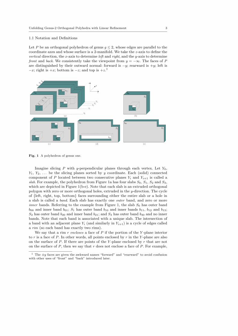
Fig. 1 A polyhedron of genus one.
Imagine slicing P with y-perpendicular planes through each vertex. Let Y0,Y1, Y2, . . . be the slicing planes sorted by y coordinate. Each (solid) connectedcomponent of P located between two consecutive planes Yi and Yi+1 is called aslab. For example, the polyhedron from Figure 1a has four slabs S0, S1, S2 and S3,which are depicted in Figure 1(b-e). Note that each slab is an extruded orthogonalpolygon with zero or more orthogonal holes, extruded in the y-direction. The cycleof {left, right, top, bottom} faces surrounding either the entire slab or a hole ina slab is called a band. Each slab has exactly one outer band, and zero or moreinner bands. Referring to the example from Figure 1, the slab S0 has outer bandb00 and inner band b01; S1 has outer band b10 and inner bands b11, b12 and b13;S2 has outer band b20 and inner band b21; and S3 has outer band b30 and no innerbands. Note that each band is associated with a unique slab. The intersection ofa band with an adjacent plane Yi (and similarly in Yi+1) is a cycle of edges calleda rim (so each band has exactly two rims).
We say that a rim r encloses a face of P if the portion of the Y -plane interiorto r is a face of P . In other words, all points enclosed by r in the Y -plane are alsoon the surface of P . If there are points of the Y -plane enclosed by r that are noton the surface of P , then we say that r does not enclose a face of P . For example,
1 The ±y faces are given the awkward names “forward” and “rearward” to avoid confusionwith other uses of “front” and “back” introduced later.
4 Mirela Damian et al.
in Figure 1 the rim of b30 in plane Y4 and the rim of b12 in plane Y2 each enclosea face of P , but the rim of b00 in Y0 does not.
2 Overview of Linear Unfolding
Throughout this section, P is an orthogonal polyhedron of genus zero. We beginwith an overview of the algorithm in [CY15] that unfolds P using linear refinement.In Section 3 we will detail those aspects of the algorithm that we modify to handleorthogonal polyhedra of genus 1 and 2.
2.1 Unfolding Extrusions
Nearly all algorithmic issues in the linear unfolding algorithm from [CY15] arepresent in unfolding polyhedra that are vertical extrusions of simple orthogonalpolygons. Therefore, we describe their unfolding algorithm for this simple shapeclass first, before extending the ideas to all orthogonal polyhedra of genus zero.
Before going into details, we briefly describe the algorithm at a high level.It begins by slicing P into slabs using y-perpendicular planes. For these verticalextrusions, all the slabs are boxes. The adjacency graph of these boxes is a tree T .Each leaf node b in T has a corresponding thin spiral surface path that includesa vertical segment running across the back face of b (which must be a face ofP ) on the side opposite to b’s parent. The surface path extends from the bottomendpoint of this vertical segment by cycling around b’s band until it reaches thetop endpoint, and from there it continues along two strands that spiral side-by-side together on P , cycling around the bands on the path in T to the root nodebox where the two strands terminate. At the root box, the endpoints of all thepairs of strands are carefully stitched together into one surface path that can beflattened in the plane as a monotone staircase. By thickening the surface pathto cover the band faces of P , and attaching the y-perpendicular faces above andbelow it, the entire surface of P is flattened without overlap into the plane. Detailsof the algorithm are provided in the sections that follow.
2.1.1 Unfolding Tree T
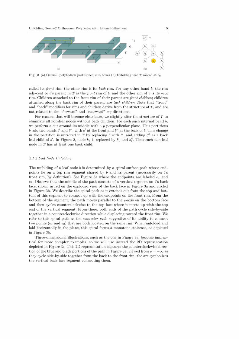
Again we restrict our attention to the situation where P is a vertical extrusionof a simple orthogonal polygon, and describe the algorithm in detail. The unfold-ing algorithm begins by slicing P with Yi planes passing through every vertex,as described in Section 1. This induces a partition of P into rectangular boxes.See Figure 2a for an example. The dual graph of this partition is a tree T whosenodes correspond to bands, and whose edges connect pairs of adjacent bands. Fig-ure 2b shows the tree T for the example from Figure 2a. We refer to T as theunfolding tree, since it will guide the unfolding process. For simplicity, we will usethe terms “node” and “band” interchangeably.
Every tree of two or more nodes has at least two nodes of degree one, sowe designate the root of T to be one of these degree-1 nodes. In Figure 2b forexample, we may choose b0 as the root of T , although any of the other degree-1nodes would serve as well. The rim of the root band that has no adjacent band is
Unfolding Genus-2 Orthogonal Polyhedra with Linear Refinement 5
Y0
Y1
Y2
Y3
Y4
b0
b9
b5
b7
b8
b6
b4b′1
b′′1
b2b3
b′′1
b4
b2 b9 b6
b5
b7
b3
b0 b8
b′1
(a) (b)
b1
b1
Fig. 2 (a) Genus-0 polyhedron partitioned into boxes (b) Unfolding tree T rooted at b0.
called its front rim; the other rim is its back rim. For any other band b, the rimadjacent to b’s parent in T is the front rim of b, and the other rim of b is its back
rim. Children attached to the front rim of their parent are front children; childrenattached along the back rim of their parent are back children. Note that “front”and “back” modifiers for rims and children derive from the structure of T , and arenot related to the “forward” and “rearward” ±y directions.
For reasons that will become clear later, we slightly alter the structure of T toeliminate all non-leaf nodes without back children. For each such internal band b,we perform a cut around its middle with a y-perpendicular plane. This partitionsb into two bands b′ and b′′, with b′ at the front and b′′ at the back of b. This changein the partition is mirrored in T by replacing b with b′, and adding b′′ as a backleaf child of b′. In Figure 2, node b1 is replaced by b′1 and b′′1 . Thus each non-leafnode in T has at least one back child.
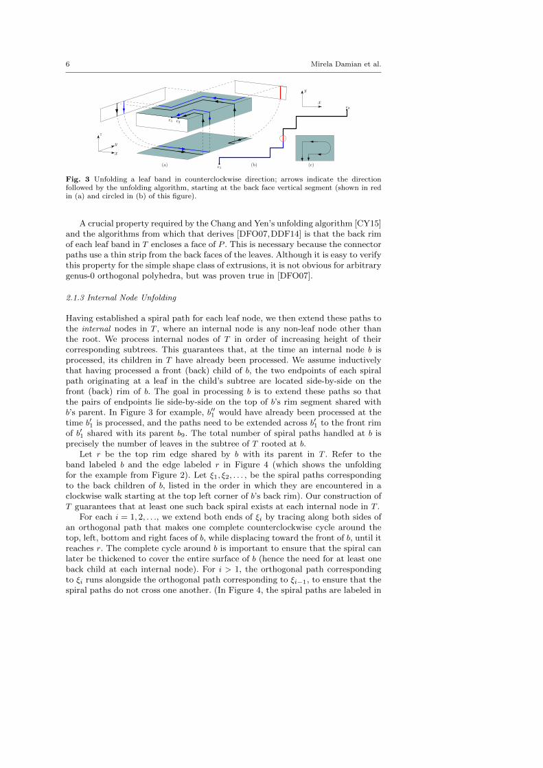
2.1.2 Leaf Node Unfolding
The unfolding of a leaf node b is determined by a spiral surface path whose end-points lie on a top rim segment shared by b and its parent (necessarily on b’sfront rim, by definition). See Figure 3a where the endpoints are labeled e1 ande2. Observe that the middle of the path consists of a vertical segment on b’s backface, shown in red on the exploded view of the back face in Figure 3a and circledin Figure 3b. We describe the spiral path as it extends out from the top and bot-tom of this segment to connect up with the endpoints on the front rim. From thebottom of the segment, the path moves parallel to the y-axis on the bottom faceand then cycles counterclockwise to the top face where it meets up with the topend of the vertical segment. From there, both ends of the path cycle side-by-sidetogether in a counterclockwise direction while displacing toward the front rim. Werefer to this spiral path as the connector path, suggestive of its ability to connecttwo points (e1 and e2) that are both located on the same rim. When unfolded andlaid horizontally in the plane, this spiral forms a monotone staircase, as depictedin Figure 3b.
Three-dimensional illustrations, such as the one in Figure 3a, become imprac-tical for more complex examples, so we will use instead the 2D representationdepicted in Figure 3c. This 2D representation captures the counterclockwise direc-tion of the blue and black portions of the path in Figure 3a, viewed from y = −∞ asthey cycle side-by-side together from the back to the front rim; the arc symbolizesthe vertical back face segment connecting them.
6 Mirela Damian et al.
x
y
z
x
y
e1 e2
(a) (b) (c)e1
e2
Fig. 3 Unfolding a leaf band in counterclockwise direction; arrows indicate the directionfollowed by the unfolding algorithm, starting at the back face vertical segment (shown in redin (a) and circled in (b) of this figure).
A crucial property required by the Chang and Yen’s unfolding algorithm [CY15]and the algorithms from which that derives [DFO07,DDF14] is that the back rimof each leaf band in T encloses a face of P . This is necessary because the connectorpaths use a thin strip from the back faces of the leaves. Although it is easy to verifythis property for the simple shape class of extrusions, it is not obvious for arbitrarygenus-0 orthogonal polyhedra, but was proven true in [DFO07].
2.1.3 Internal Node Unfolding
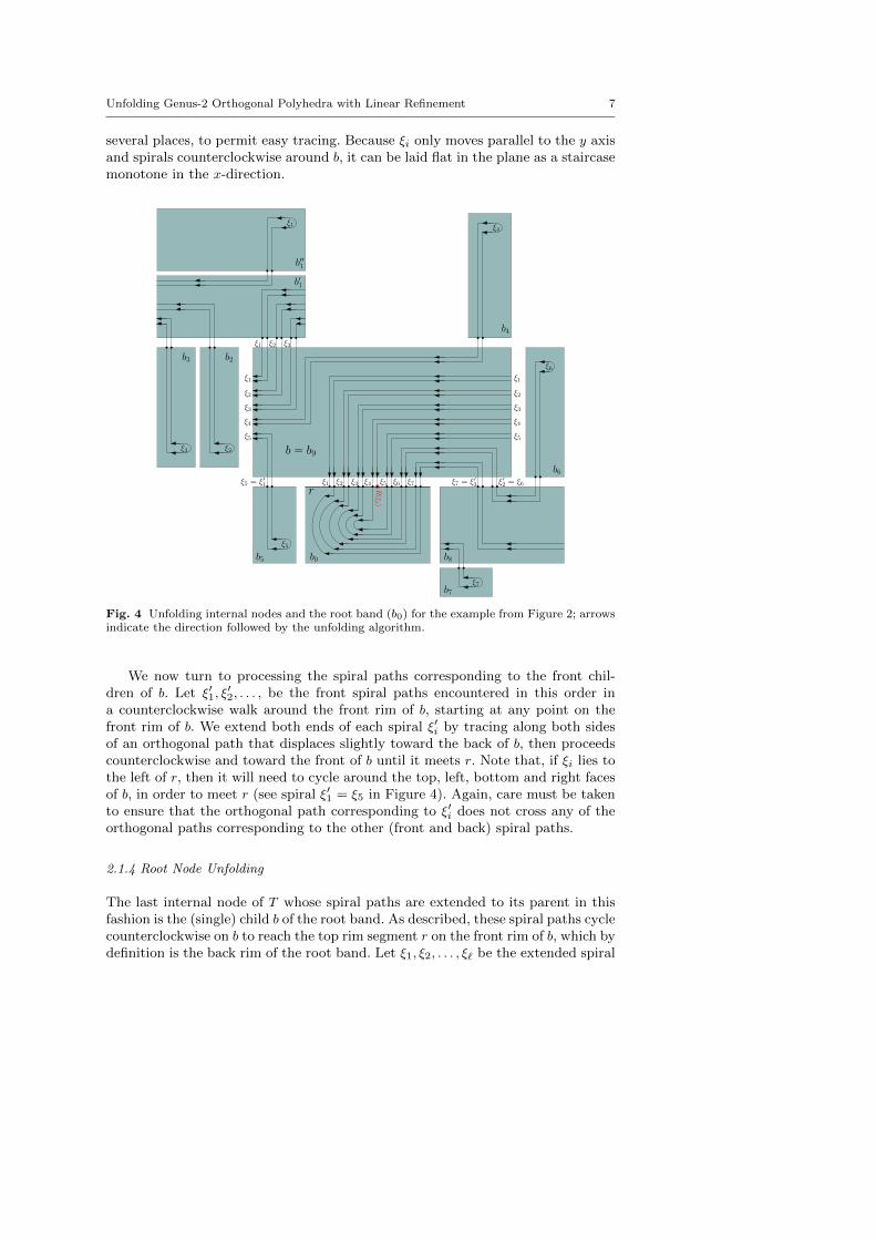
Having established a spiral path for each leaf node, we then extend these paths tothe internal nodes in T , where an internal node is any non-leaf node other thanthe root. We process internal nodes of T in order of increasing height of theircorresponding subtrees. This guarantees that, at the time an internal node b isprocessed, its children in T have already been processed. We assume inductivelythat having processed a front (back) child of b, the two endpoints of each spiralpath originating at a leaf in the child’s subtree are located side-by-side on thefront (back) rim of b. The goal in processing b is to extend these paths so thatthe pairs of endpoints lie side-by-side on the top of b’s rim segment shared withb’s parent. In Figure 3 for example, b′′1 would have already been processed at thetime b′1 is processed, and the paths need to be extended across b′1 to the front rimof b′1 shared with its parent b9. The total number of spiral paths handled at b isprecisely the number of leaves in the subtree of T rooted at b.
Let r be the top rim edge shared by b with its parent in T . Refer to theband labeled b and the edge labeled r in Figure 4 (which shows the unfoldingfor the example from Figure 2). Let ξ1, ξ2, . . . , be the spiral paths correspondingto the back children of b, listed in the order in which they are encountered in aclockwise walk starting at the top left corner of b’s back rim). Our construction ofT guarantees that at least one such back spiral exists at each internal node in T .
For each i = 1, 2, . . ., we extend both ends of ξi by tracing along both sides ofan orthogonal path that makes one complete counterclockwise cycle around thetop, left, bottom and right faces of b, while displacing toward the front of b, until itreaches r. The complete cycle around b is important to ensure that the spiral canlater be thickened to cover the entire surface of b (hence the need for at least oneback child at each internal node). For i > 1, the orthogonal path correspondingto ξi runs alongside the orthogonal path corresponding to ξi−1, to ensure that thespiral paths do not cross one another. (In Figure 4, the spiral paths are labeled in
Unfolding Genus-2 Orthogonal Polyhedra with Linear Refinement 7
several places, to permit easy tracing. Because ξi only moves parallel to the y axisand spirals counterclockwise around b, it can be laid flat in the plane as a staircasemonotone in the x-direction.
ξ1
ξ3 ξ2
ξ4
ξ5
ξ7
ξ6
ξ3ξ1 ξ2
ξ3ξ1 ξ2 ξ4 ξ5 ξ6 ξ7 ξ7 = ξ′3 ξ′2 = ξ6ξ5 = ξ′1r
b = b9
ξ1
ξ2
ξ3
ξ4
ξ5
ξ1
ξ2
ξ3
ξ4
ξ5
b0b5 b8
b7
b6
b4
b′1
b′′1
b2b3
R(ξ
4 )
Fig. 4 Unfolding internal nodes and the root band (b0) for the example from Figure 2; arrowsindicate the direction followed by the unfolding algorithm.
We now turn to processing the spiral paths corresponding to the front chil-dren of b. Let ξ′1, ξ
′2, . . . , be the front spiral paths encountered in this order in
a counterclockwise walk around the front rim of b, starting at any point on thefront rim of b. We extend both ends of each spiral ξ′i by tracing along both sidesof an orthogonal path that displaces slightly toward the back of b, then proceedscounterclockwise and toward the front of b until it meets r. Note that, if ξi lies tothe left of r, then it will need to cycle around the top, left, bottom and right facesof b, in order to meet r (see spiral ξ′1 = ξ5 in Figure 4). Again, care must be takento ensure that the orthogonal path corresponding to ξ′i does not cross any of theorthogonal paths corresponding to the other (front and back) spiral paths.
2.1.4 Root Node Unfolding
The last internal node of T whose spiral paths are extended to its parent in thisfashion is the (single) child b of the root band. As described, these spiral paths cyclecounterclockwise on b to reach the top rim segment r on the front rim of b, which bydefinition is the back rim of the root band. Let ξ1, ξ2, . . . , ξ` be the extended spiral

8 Mirela Damian et al.
paths listed in the order encountered in a clockwise walk around the front rim of b,starting at the top left corner of the root’s back face. Here ` is the number of leafnodes in T . (For example, ` = 7 in the example from Figure 4.) Let L(ξi) be the leftendpoint of spiral ξi on r and let R(ξi) be the right endpoint. With this notation,the endpoints from left to right on r are L(ξ1), R(ξ1), L(ξ2), R(ξ2), . . . , L(ξ`), R(ξ`).
The next step of the algorithm is to link these ` spiral paths into a singlepath ξ that can be flattened in the plane as a monotone staircase. The startingpoint of ξ is L(ξ1), and the first part of ξ consists of ξ1 followed by ξ`. Thesetwo spiral paths are linked via a connector path on the root band that extendsfrom endpoint R(ξ1) to endpoint R(ξ`). See the 2D representation of the connectorpath linking the right endpoint of ξ1 to the right endpoint of ξ7 in Figure 4. Thisconnector path is analogous to the connector paths followed at the leaf nodes,but here the vertical segment is on the front face of the root band. Because theroot node has degree one and its only child is adjacent on its back rim, the root’sfront rim encloses a face of P , and so it is possible for the path to connect in thismanner. This connector path is depicted in Figure 5. From R(ξ`), the connectorpath cycles counterclockwise to reach R(ξ1). From there, both parts of the path(i.e., the extensions of R(ξ`) and R(ξ1)) cycle counterclockwise together towardsthe front face. The part of the path extending from R(ξ`) meets the front facevertical segment at its top endpoint, while the other part of the path extendingfrom R(ξ1) continues cycling to the bottom face and meets the vertical segment atits bottom endpoint. (Observe that this path is a mirror image of the one depictedin Figure 3.) Like a leaf node connector path, this path can be laid flat in the
x
y
z
R(ξ1)R(ξ`)
Fig. 5 The connector path for the spiral paths ξ1 and ξ`; arrows indicate the direction followedby the unfolding algorithm, up to the vertical segment on the front face.
plane as a monotone staircase. Because the counterclockwise cycling direction ofthe connector path is consistent with that of ξ1 and ξ`, ξ1 can be laid flat on oneside of the path and ξ` can be laid flat on the other side, thus forming a singlemonotone staircase. In this way we link ξ1 and ξ` to form the first part of ξ.
Continuing to link the spiral paths to form ξ, L(ξ`) is linked to endpoint L(ξ2)using a connector path that runs alongside the previous connector path. Similarly,this connector path flattens to a monotone staircase and connects the two flattenedstaircases ξ` and ξ2. The remaining endpoints are paired up similarly and linkedwith connector paths. Specifically, R(ξi) is linked to R(ξ`−i+1) and L(ξi) is linkedto L(ξ`−i+2)), for i = 2, 3, . . . until one unpaired endpoint remains: L(ξ`/2+1) (if `is even) or R(ξ(`+1)/2) (if ` is odd). This endpoint is where ξ terminates. See R(ξ4)in Figure 4.
Unfolding Genus-2 Orthogonal Polyhedra with Linear Refinement 9
2.1.5 Completing the Unfolding
To complete the unfolding of P , the spiral ξ is thickened in the +y and −y directionso that it completely covers each band. This results in a thicker strip, which canbe unfolded as a staircase in the plane. Then the forward and rearward faces ofP are partitioned by imagining the band’s top rim edges illuminating downwardlight rays in these faces. The illuminated pieces are then “hung” above and belowthe thickened staircase, along the corresponding illuminating rim segments thatlie along the horizontal edges of the staircase.
2.2 Unfolding Genus-0 Orthogonal Polyhedra
The unfolding algorithm described in subsection 2.1 for extrusions generalizes toall genus-0 orthogonal polyhedra as described in [CY15], so we briefly present themain ideas here and refer the reader to [CY15] for details.
Instead of partitioning P into boxes, the unfolding algorithm partitions P intoslabs as defined in Section 1. It then creates an unfolding tree T in which eachnode corresponds to either an outer band (surrounding a slab) or an inner band(surrounding a hole). Each edge in T corresponds to a z-beam, which is a thinvertical rectangular strip from a frontward or rearward face of P connecting aparent’s rim to a child’s rim. Note that a z-beam may have zero geometric height,when two rims share a common segment. The spiral paths connect vertically alongthe z-beams when transitioning from a child band to its parent. For a parent bandb, its front (back) children are those whose z-beams connect to b’s front (back) rim.It was established in [DFO07] that the back rim of each leaf node in T encloses aface of P .
2.2.1 Assigning Unfolding Directions
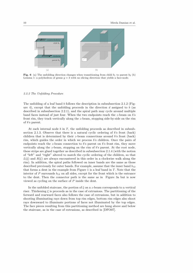
Unlike the case of protrusions, where all bands are unfolded in the same direction(i.e., either all counterclockwise or all clockwise), general genus-0 orthogonal poly-hedra may require different unfolding directions for different bands. For example,if a z-beam is incident to a top rim edge of the parent and a bottom rim edgeof the child, then the unfolding direction (viewed from y = −∞) changes whentransitioning from the child to the parent. Figure 6a shows such an example.
We assign unfolding directions for each band in a preorder traversal of theunfolding tree T . Set the unfolding direction for the root band to counterclockwise.At each band node b visited in a preorder traversal of T , if the edge in T connectingb to its parent corresponds to a z-beam incident to both top and bottom rim points,then set the unfolding direction for b to be opposite to the one for the parent (i.e.,if the unfolding direction for the parent is counterclockwise, then the unfoldingdirection for b will be clockwise, and vice versa.) Otherwise, the endpoints of thez-beam connecting b to its parent are both top rim points or both bottom rimpoints, and in that case b inherits the unfolding direction of its parent. (Recallthat a z-beam can have zero geometric height where two rims overlap.)
10 Mirela Damian et al.
clockwise
counterclockwise
parent b2
(a) (b)
child b1
Fig. 6 (a) The unfolding direction changes when transitioning from child b1 to parent b2 (b)Lemma 1: a polyhedron of genus g = 3 with no slicing direction that yields a face-node.
2.2.2 The Unfolding Procedure
The unfolding of a leaf band b follows the description in subsubsection 2.1.2 (Fig-ure 4), except that the unfolding proceeds in the direction d assigned to b (asdescribed in subsubsection 2.2.1), and the spiral path may cycle around multipleband faces instead of just four. When the two endpoints reach the z-beam on b’sfront rim, they track vertically along the z-beam, stopping side-by-side on the rimof b’s parent.
At each internal node b in T , the unfolding proceeds as described in subsub-section 2.1.3. Observe that there is a natural cyclic ordering of b’s front (back)children that is determined by their z-beam connections around b’s front (back)rim, which guides the order in which we process b’s children. Once the pairs ofendpoints reach the z-beam connection to b’s parent on b’s front rim, they movevertically along the z-beam, stopping on the rim of b’s parent. At the root node,these strips are glued together as described in subsubsection 2.1.4 (with the notionof “left” and “right” altered to match the cyclic ordering of the children, so thatL(ξ) and R(ξ) are always encountered in this order in a clockwise walk along therim). In addition, the spiral paths followed on inner bands are the same as thosedescribed previously for outer bands. For example, assume that the inner band b12that forms a dent in the example from Figure 1 is a leaf band in T . Note that theinterior of P surrounds b12 on all sides, except for the front which is the entranceto the dent. Then the connector path is the same as in Figure 3a but is nowviewed as cycling on the surface of P inside the dent.
In the unfolded staircase, the portion of ξ on a z-beam corresponds to a verticalriser. Thickening ξ is proceeds as in the case of extrusions. The partitioning of theforward and rearward faces also follows the case of extrusions, but in addition toshooting illuminating rays down from top rim edges, bottom rim edges also shootrays downward to illuminate portions of faces not illuminated by the top edges.The face pieces resulting from this partitioning method are hung above and belowthe staircase, as in the case of extrusions, as described in [DFO07].
Unfolding Genus-2 Orthogonal Polyhedra with Linear Refinement 11
3 Unfolding Genus-2 Orthogonal Polyhedra
The unfolding algorithm described in Section 2 depends on two key propertiesof P that are not necessarily true if P has genus 1 or 2. First, it requires theexistence of a band with a rim enclosing a face of P that can serve as the rootnode of T . And second, it requires the back rim of each leaf node in T to enclosea face of P . These two requirements are needed so that the connector paths canuse vertical strips on the enclosed faces in the unfolding. As a simple example ofa genus-1 polyhedron for which neither property holds, consider the case when P
is a box with a y-parallel hole through its middle. Slicing P with y-perpendicularplanes results in a single slab having one outer and one inner band. In this case,no rim encloses a face of P . If we rotate P so that the hole is parallel to the x axisinstead, slicing produces four bands, and the band surrounding the frontward (orrearward) box could serve as the root node. But every unfolding tree for the fourbands contains a leaf whose back rim doesn’t enclose a face of P .
In this section, we first show that there always exists an orientation for P suchthat at least one band has a rim enclosing a face of P that can be used for the rootof T . Then we describe an algorithm that computes an unfolding tree for whichwe can prove that the number of leaf bands whose back rims do not enclose a faceof P is at most g, where g is the genus of P . Finally, we describe changes to theunfolding algorithm that allow it to handle up to g leaves that don’t enclose a faceof P , for g ≤ 2.
3.1 The Rim Unfolding Tree Tr
In order to establish these new results, we need finer-grained structures than theband-based G and T , which we call Gr and Tr, both of which are rim-based. Wedefine the rim graph Gr for P in the following way. For each band b of P , add twonodes rb and r′b to Gr corresponding to each of b’s rims. Add an edge connecting rband r′b and call it a band edge, or a b-edge for short. For each pair of rims that can beconnected by a z-beam, add an edge between them in Gr, and call it a z-beam edge,or a z-edge for short. When referring to Gr, we will use the terms node and riminterchangably. For any simple cycle C in Gr, we distinguish between b-nodes ofC, which are endpoints of b-edges in C, and z-nodes of C, incident to two adjacentz-edges in C. For any subgraph J ⊆ Gr, we use V (J) and E(J) to denote the setof nodes and the set of edges in J , respectively.
Call a rim of Gr that encloses a face of P a face-node. A nonface-node in Gr isa node whose rim does not enclose a face of P .
Proposition 1 A rim r is a face-node of Gr if and only if every z-beam extending
from a horizontal edge of r and going up or down on the surface of P hits r. A face-node
of Gr is necessarily of degree one.
Lemma 1 If polyhedron P has genus g ≤ 2, then there is a direction for slicing P
such that Gr includes a face-node rF .
Proof Define the extreme faces of P as those faces flush with the smallest bound-ing box enclosing P . There must be at least one extreme face in each of the sixdirections d ∈ {±x,±y,±z}. If any extreme face F , say in direction d, is simply
12 Mirela Damian et al.
connected, then slicing P with a d-plane (parallel to F ) just adjacent to F willcreate a band b one of whose rims rF encloses F . Thus, slicing P with d-planeswill result in Gr including the face-node rF , and the lemma is established.
Assume henceforth that each of the at least six extreme faces of P is notsimply connected. So each extreme face F includes at least one inner band b. Wenow classify these bands b into two types.
Let r be the rim of an inner band b in face F . If cutting along r separates thesurface of P into two pieces, P ′ which includes b, and the remainder P \ P ′, thenwe say that b is a cave-band. Let M be the “mouth” of the cave: the portion ofthe Y -plane enclosed by the rim r. P ′ is a “cave” in the sense that an exteriorpath that enters through M can only exit P ′ back through M again. A band b
that is not a cave-band is a hole-band. These have the property that there is anexterior topological circle that passes through the mouth M once, and so exits P ′
elsewhere.
Let P ′ be a cave with mouth M . P ′ ∪ M is an orthogonal polyhedron P ′M ,inverting what was exterior to P to become interior to P ′M . Say that cave P ′ hasgenus 0 if P ′M has genus 0. We now claim that the lemma is satisfied if P has agenus-0 cave. For we may apply the same procedure to P ′M : Examine its extremefaces (one of which is M). If any extreme face (other than M) is simply connected,we are finished. Otherwise, each extreme face includes an inner band b′. It cannotbe the case that b′ is a hole band, for then P ′M has genus greater than 1. Moreover,b′ cannot be a cave band for a cave of genus greater than 1. For in both cases, wecould cut a cycle on the surface of P ′ that would not disconnect P ′. So b′ mustdetermine a genus-0 cave band, and the argument repeats. Eventually we reach asimply connected extreme face.
Now we have reduced to the situation that each of P ’s six or more extremefaces contains either a hole-band, or a genus-(≥ 1) cave band. Let the number ofthese bands be h and c respectively. We now account for the the genus g of P , andthe number of extreme faces. Each cave of genus-(≥ 1) contributes at least 1 to g.A hole-band in an extreme face could exit through that same face, or exit througha different extreme face, or exit through a non-extreme face. In the first two cases,two hole-bands contribute 1 to g; in the third case, one hole band contributes 1 tog. So h hole-bands contribute at least h/2 to the genus, and we have the inequalityc+ h/2 ≤ g ≤ 2.
We have defined h and c to be the number of such bands in extreme faces, andwe know that each of the at least six extreme faces must have one or more hole-or genus-(≥ 1) cave-bands. So we must have c+ h ≥ 6. But these two inequalitieshave no solutions in non-negative integers. ut
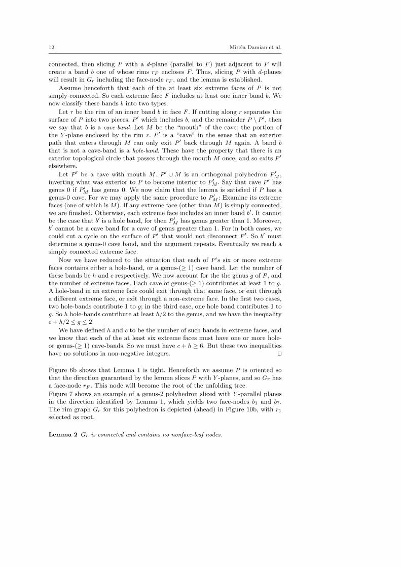
Figure 6b shows that Lemma 1 is tight. Henceforth we assume P is oriented sothat the direction guaranteed by the lemma slices P with Y -planes, and so Gr hasa face-node rF . This node will become the root of the unfolding tree.
Figure 7 shows an example of a genus-2 polyhedron sliced with Y -parallel planesin the direction identified by Lemma 1, which yields two face-nodes b1 and b7.The rim graph Gr for this polyhedron is depicted (ahead) in Figure 10b, with r1selected as root.
Lemma 2 Gr is connected and contains no nonface-leaf nodes.
Unfolding Genus-2 Orthogonal Polyhedra with Linear Refinement 13
b1 b2
b3
b4
b5 b6b7
Y0
Y1
Y2
Y3
Y4
Y5
r1
r′1
r3
r2
r′2
r′3
Y0
Y1
Y1
Y2
r4
Y2
Y3
r5
r′5
Y3
Y4
r′4r6
r′6
r7
Y4
Y5
r′7
b1 b2
b3
b4b5 b6 b7
Fig. 7 Genus-2 polyhedron partitioned into slabs.
Proof Call a maximal connected surface piece of P located in a plane Yi a z-patch
(suggestive of the fact that it might contain z-beams). First note that the subset ofrims belonging to a z-patch induce a connected component in Gr (call it a z-patch
component) that contains z-edges only. The connectedness of P ’s surface impliesthat all z-patches are connected together by bands. In Gr, this corresponds toall z-patch components being connected together by b-edges. It follows that Gr isconnected.
Next we show that there are no nonface-leaves in Gr. Suppose there is a noder in Gr of degree 1 that does not enclose a face of P . Because all nodes in Gr
are connected by a b-edge to the rim on the other side of the band, there is ab-edge adjacent to r. Now consider extending z-beams up and down from everyhorizontal edge of r. Because r does not enclose a face of P , at least one of thez-beams must hit the rim of another band by Proposition 1. But then r also hasa z-edge adjacent to it, giving it a degree of at least 2, a contradiction. ut
Note that Gr for the genus-3 example in Figure 6b has no leaf nodes at all, andso satisfies this lemma vacuously.
Our next goal is to find a rim spanning tree Tr of Gr with at most g nonface-leaves, which will ultimately similarly limit the number of nonface-leaf nodes ofT . The RimUnfoldingTree method for achieving such a Tr is outlined in Algo-rithm 1. It reduces Gr to a tree by repeatedly removing a z-edge from an existingcycle, thus breaking the cycle. In addition, it does this in such a way that at mostg nonface-leaf nodes are created. If we were to break a cycle by removing an arbi-trary z-edge from it, it may be that both endpoints of the z-edge have degree two,and thus removing it would result in the creation of two new leaf nodes, both ofwhich would be nonface-nodes. To avoid this, our RimUnfoldingTree algorithmstrategically selects a z-edge e with at least one endpoint, say u, of degree 3 or
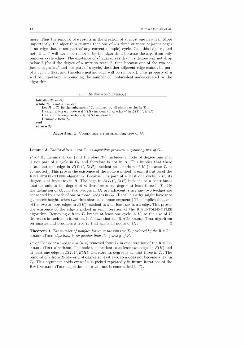
14 Mirela Damian et al.
more. Thus the removal of e results in the creation of at most one new leaf. Moreimportantly, the algorithm ensures that one of u’s three or more adjacent edgesis an edge that is not part of any current (simple) cycle. Call this edge e′, andnote that e′ will never be removed by the algorithm, because the algorithm onlyremoves cycle edges. The existence of e′ guarantees that u’s degree will not dropbelow 2 (for if the degree of u were to reach 2, then because one of the two ad-jacent edges is e′ and not part of a cycle, the other adjacent edge cannot be partof a cycle either, and therefore neither edge will be removed). This property of uwill be important in bounding the number of nonface-leaf nodes created by thealgorithm.
Tr = RimUnfoldingTree(Gr)
Initialize Tr ← Gr
while Tr is not a tree doLet H ⊂ Tr be the subgraph of Tr induced by all simple cycles in TrPick an arbitrary node u ∈ V (H) incident to an edge e′ in E(Tr) \ E(H)Pick an arbitrary z-edge e ∈ E(H) incident to uRemove e from Tr
endreturn Tr
Algorithm 1: Computing a rim spanning tree of Gr.
Lemma 3 The RimUnfoldingTree algorithm produces a spanning tree of Gr.
Proof By Lemma 1, Gr (and therefore Tr) includes a node of degree one thatis not part of a cycle in Gr and therefore is not in H. This implies that thereis at least one edge in E(Tr) \ E(H) incident to a node u of H (because Tr isconnected). This proves the existence of the node u picked in each iteration of theRimUnfoldingTree algorithm. Because u is part of a least one cycle in H, itsdegree is at least two in H. The edge in E(Tr) \ E(H) incident to u contributesanother unit to the degree of u; therefore u has degree at least three in Tr. Bythe definition of Gr, no two b-edges in Gr are adjacent, since any two b-edges areconnected by a path of one or more z-edges in Gr. (Recall a z-edge might have zerogeometric height, when two rims share a common segment.) This implies that, outof the two or more edges in E(H) incident to u, at least one is a z-edge. This provesthe existence of the edge e picked in each iteration of the RimUnfoldingTree
algorithm. Removing e from Tr breaks at least one cycle in H, so the size of Hdecreases in each loop iteration. It follows that the RimUnfoldingTree algorithmterminates and produces a tree Tr that spans all nodes of Gr. ut
Theorem 1 The number of nonface-leaves in the rim tree Tr produced by the RimUn-
foldingTree algorithm is no greater than the genus g of P .
Proof Consider a z-edge e = (u, v) removed from Tr in one iteration of the RimUn-
foldingTree algorithm. The node u is incident to at least two edges in E(H) andat least one edge in E(Tr) \E(H); therefore its degree is at least three in Tr. Theremoval of e from Tr leaves u of degree at least two, so u does not become a leaf inTr. This argument holds even if u is picked repeatedly in future iterations of theRimUnfoldingTree algorithm, so u will not become a leaf in Tr.
Unfolding Genus-2 Orthogonal Polyhedra with Linear Refinement 15
If v has degree three or more in Tr prior to removing e from Tr, then v doesnot become a leaf after removing e. So suppose that v has degree two in Tr beforeremoving e. Recall that every node in Gr is connected by a b-edge to the other rimof its band. Because the RimUnfoldingTree algorithm never removes a b-edge,this property holds in Tr as well. It follows that the other edge incident to v (inaddition to the z-edge e) must be a b-edge. Hence any leaf node in Tr created bythe RimUnfoldingTree algorithm is an endpoint of a b-edge in Tr.
By Lemma 2, Gr does not include any nonface-leaves, so any nonface-leaves inTr must have been created by the RimUnfoldingTree algorithm. Let r1, r2, . . . , rkbe the set of leaves in Tr created by the RimUnfoldingTree algorithm. If k ≤ g,then the theorem is true.
b1
b2
b3
b5
r4
(a) (b)
c′2c2
c′1c1
γ1
γ2
r1
b8
b7
b6
r′1
r3
r′3
r1 r4
r′1 r′4
r5
r′5
r2 r6
r′2 r′6
r7
r′7
r8
r′8
e1 = (r1, r′3)
r′3 = u1
r3
b4
r′4
r5
r′5
r6
r′6
r7
r′7
r2
r′2
r8
u2 = r′8e2 = (r2, r
′8)
e2
e1
p1
p2
Fig. 8 Theorem 1 (a) example polyhedron of genus 2; cuts around the middle of bands b1 andb2 are marked with dashed lines (b) Rim tree Tr with root r3 and 2 nonface-leaves, r1 and r2.
Assume now that k > g. For each i, let bi be the band with rim ri. BecauseTr includes all the b-edges from Gr, it must be that Tr includes the b-edge (ri, r
′i)
corresponding to bi, so the parent r′i of ri in Tr is the other rim of bi. For eachi = 1, 2, . . . , k, we perform a cut on P ’s surface along a closed curve around themiddle of bi, between its rims ri and r′i. Refer to Figure 8a, which shows the cutsaround the middle of b1 and b2 as dashed lines. Note that r1 and r2 are nonface-nodes corresponding to b1 and b2 respectively, as inferred from the rim unfoldingtree Tr shown in Figure 8b (edges of Tr are marked solid, with b-edges thickerthan z-edges). We now show that these cuts do not disconnect the surface of P ,contradicting our assumption that k > g.
To see this, consider any two points ci and c′i on bi that are separated by thecut around bi, with ci on the same side of the cut as ri, and c′i on the same sideof the cut as r′i. Let ei = (ri, ui) be the z-edge whose removal from Tr created theleaf ri (so ui here plays the role of u in the RimUnfoldingTree algorithm, andby our observation above, ui is not a leaf in Tr). We construct a path pi on thesurface of P connecting ci to c′i as follows: the path pi starts at ci, moves towardsri and along the z-beam corresponding to ei to the rim ui, then follows the pathin Tr from ui to the rim r′i, and finally across bi to c′i. See Figure 8, which tracesthe paths p1 and p2 on the polyhedron surface. Note that ri is the only leaf visited
16 Mirela Damian et al.
by pi (because ui is not a leaf), so pi does not cut across any of the leaves rj , forj 6= i. This implies that pi connects ci and c′i in the presence of all the other cutspj , with j 6= i. Since this is true for each i, we conclude that these cuts leave thesurface of P connected, contradicting our assumption that k > g. ut
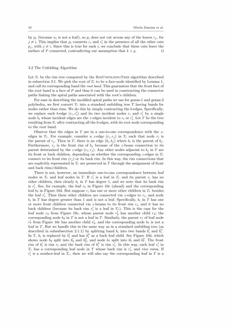
3.2 The Unfolding Algorithm
Let Tr be the rim tree computed by the RimUnfoldingTree algorithm describedin subsection 3.1. We pick the root of Tr to be a face-node identified by Lemma 1,and call its corresponding band the root band. This guarantees that the front face ofthe root band is a face of P and thus it can be used in constructing the connectorpaths linking the spiral paths associated with the root’s children.
For ease in describing the modified spiral paths we use for genus-1 and genus-2polyhedra, we first convert Tr into a standard unfolding tree T having bands fornodes rather than rims. We do this by simply contracting the b-edges. Specifically,we replace each b-edge (ri, r
′i) and its two incident nodes ri and r′i by a single
node bi whose incident edges are the z-edges incident to ri or r′i. Let T be the treeresulting from Tr after contracting all the b-edges, with its root node correspondingto the root band.
Observe that the edges in T are in a one-to-one correspondence with the z-edges in Tr. For example, consider a z-edge (ri, rj) in Tr such that node ri isthe parent of rj . Then in T , there is an edge (bi, bj) where bi is the parent of bj .Furthermore, rj is the front rim of bj because of the z-beam connection to itsparent determined by the z-edge (ri, rj). Any other nodes adjacent to bj in T areits front or back children, depending on whether the corresponding z-edges in Trconnect to its front rim (rj) or its back rim. In this way, the rim connections thatare explicitly represented in Tr are preserved in T through the assignment of frontand back rims/children.
There is not, however, an immediate one-to-one correspondence between leafnodes in Tr and leaf nodes in T . If r′i is a leaf in Tr and its parent ri has noother children, then clearly bi in T has degree 1, and we note that its back rimis r′i. See, for example, the leaf r5 in Figure 10c (ahead) and the correspondingleaf b5 in Figure 10d. But suppose ri has one or more other children in Tr besidesthe leaf r′i. Then these other children are connected via z-edges to ri, and nodebi in T has degree greater than 1 and is not a leaf. Specifically, bi in T has oneor more front children connected via z-beams to its front rim ri, and it has noback children (because its back rim r′i is a leaf in Tr). This is the case for theleaf node r2 from Figure 10c, whose parent node r′2 has another child r4; thecorresponding node b2 in T is not a leaf in T . Similarly, the parent r7 of leaf noder′7 from Figure 10c has another child r′5, and the corresponding node b7 is not aleaf in T . But we handle this in the same way as in a standard unfolding tree (asdescribed in subsubsection 2.1.1) by splitting band bi into two bands b′i and b′′i .In T , bi is replaced by b′i and has b′′i as a back leaf child. See Figure 10d, whichshows node b2 split into b′2 and b′′2 , and node b7 split into b′7 and b′′7 . The frontrim of b′i is rim ri and the back rim of b′′i is rim r′i. In this way, each leaf r′i inTr has a corresponding leaf node in T whose back rim is r′i, and vice versa. Ifr′i is a nonface-leaf in Tr, then we will also say the corresponding leaf in T is a
Unfolding Genus-2 Orthogonal Polyhedra with Linear Refinement 17
nonface-leaf, meaning that its band’s back rim does not enclose a face of P . Theseobservations, along with Theorem 1, establish the following corollary.
Corollary 1 The number of nonface-leaves in the unfolding tree T is at most g, where
g ≥ 0 is the genus of P .
Using T , we assign unfolding directions to each band as described in subsub-section 2.2.1. If T has no nonface-leaves, then we complete the unfolding of Pusing the linear unfolding algorithm from [CY15] (as summarized in Section 2).We now show how to modify the unfolding algorithm to handle the cases when T
has one or two nonface-leaves. Because a nonface-leaf b has a back rim that doesnot enclose a face of P , there might be no vertical back face segment available forb’s connector path. For these leaves, we use a spiral path that has one endpoint onb’s back rim and the other endpoint on b’s front rim. The path cycles around theband faces in the unfolding direction of b from the back point to the front point.(In Figure 3, this would be just the portion of the path that extends from the topof the back rim to endpoint e1.) Corollary 1 implies that this can occur for at mosttwo leaves in T (since we assume P to have genus g ≤ 2). For all face-leaves, weproceed as before in extending both ends of the spiral path from the band’s backrim to its front rim.
The processing of internal nodes is handled as before by extending the spiralpaths towards the root. The only difference is that for the (at most 2) spiral pathsoriginating at nonface-leaves, there is only one end of the path to extend. Afterprocessing the internal nodes, the ends of the spiral paths are at the root band.Specifically, each spiral path originating at a face-leaf has two endpoints locatedon the back rim of the root band, and each spiral path originating at a nonface-leafhas one endpoint located on the back rim of the root band. The challenge here is toconnect all these spiral paths together at the root band into a single final strip thatstarts on the back rim of one nonface-leaf and (if there is a second nonface-leaf)ends on the back rim of the other. (This is one place where the assumption thatg ≤ 2, and so there are at most two nonface-leaves (by Corollary 1), is crucial.)Because the front rim of the root node does enclose a face of P , it is possible touse strips from its enclosed face for the connectors.
3.2.1 Root Node Unfolding: One Nonface-Leaf Case
First we describe how to link the leaves’ extended spiral paths together at the rootnode, and unfold the root band in the process, for the case when T has exactly onenonface-leaf. Let ξ1, ξ2, ..., ξ` be the spiral paths corresponding to the ` face-leavesin T (excluding the one nonface-leaf). After processing all the internal nodes, thetwo ends of each of these spiral paths are located side-by-side on the back rim r
of the root band, as previously illustrated in Figure 4. Let t be the spiral pathcorresponding to the nonface-leaf. One end of t is on r, and the other end is onthe back rim of its leaf. If ` > 1, we assume the spiral paths of the face-leavesare labeled in clockwise order around the root’s back rim, with t located in themiddle between ξd`/2e and ξd`/2e+1. We then begin by linking all these spiral pathsinto one strip ξ as described in subsubsection 2.1.4 for the case when there are nononface-leaves. I.e., starting with the pair R(ξ1) and R(ξ`), the ends of the spiralpaths are paired up and linked together via connector paths. (Recall that, for each
18 Mirela Damian et al.
ξi, the endpoints L(ξi) and R(ξi) are encountered in this order in a clockwise walkalong the back rim of the root band, starting, say, at t or at a rim corner.) Theonly difference is that, with t in the middle between ξ1 and ξ`, the last pair ofspiral path endpoints linked together will be R(ξd`/2e) and t when ` is odd, and t
and L(ξd`/2e+1) when ` is even. The remainder of the unfolding is the same. Thusthe resulting spiral ξ starts at L(ξ1) and ends on the back rim of the nonface-leaf.
3.2.2 Root Node Unfolding: Two Nonface-Leaves Case
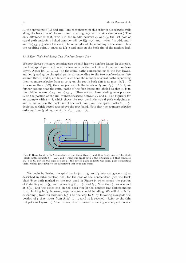
We now discuss the more complex case when T has two nonface-leaves. In this case,the final spiral path will have its two ends on the back rims of the two nonface-leaves. Again let ξ1, ξ2, ..., ξ` be the spiral paths corresponding to the face-leaves,and let t1 and t2 be the spiral paths corresponding to the two nonface-leaves. Weassume that t1 and t2 are labeled such that the number of spiral paths separatingthem counterclockwise from t2 to t1 on the root’s back rim is at most b`/2c. (Ifit is more than b`/2c, then we just switch the labels of t1 and t2.) If ` > 1, wefurther assume that the spiral paths of the face-leaves are labeled so that t1 is inthe middle between ξd`/2e and ξd`/2e+1. Observe that these labeling rules positiont2 on the portion of the rim counterclockwise between ξ1 and t1. See Figure 9 foran example with ` = 4, which shows the root band, the spiral path endpoints t1and t2 marked on the back rim of the root band, and the spiral paths ξ1, . . . ξ4depicted as thick dotted arcs above the root band. Note that the counterclockwiseordering from ξ1 along the rim is: ξ1, . . . , t2, . . . , t1.
x
y
ξ1 ξ2 t1 ξ3 ξ4t2
K
eL(ξ
1)
R(ξ
1)
L(ξ
4)
R(ξ
4)
Fig. 9 Root band, with ξ consisting of the thick (black) and thin (red) paths. The thick(black) path connects ξ1, . . . , ξ4 and t1. The thin (red) path is the extension of ξ that connectsL(ξ1) to t2. For the two ends of each ξi, the dotted paths indicate the spiral path connectingthem, which goes down to the associated leaf node and back.
We begin by linking the spiral paths ξ1, . . . , ξ` and t1 into a single strip ξ asdescribed in subsubsection 3.2.1 for the case of one nonface-leaf. (See the thickblack/blue path marked on the root band in Figure 9, which shows the portionof ξ starting at R(ξ1) and connecting ξ1, . . . ξ4 and t1.) Note that ξ has one endat L(ξ1) and the other end on the back rim of the nonface-leaf correspondingto t1. Linking in t2, however, requires some special handling. We will do this byextending ξ from its endpoint L(ξ1) all the way to t2 by following alongside theportion of ξ that tracks from R(ξ1) to t1, until t2 is reached. (Refer to the thinred path in Figure 9.) At all times, this extension is tracing a new path on one
Unfolding Genus-2 Orthogonal Polyhedra with Linear Refinement 19
side of the path it is following. Specifically, starting from L(ξ1), the extensionfirst follows alongside the connector path linking R(ξ1) to R(ξ`). It then followsalongside the spiral path from R(ξ`) to L(ξ`), going all the way down to the leafnode corresponding to ξ` and then back up. It next follows alongside the connectorpath linking L(ξ`) to L(ξ2), and then alongside the spiral path from L(ξ2) to R(ξ2),and so on. This continues until the extension reaches the connector path, say K,that links to the end of the strip piece located immediately counterclockwise fromt2 on the rim. This connector is drawn blue in Figure 9. Because at most b`/2cspiral paths are located counterclockwise from t2 to t1, the strip piece locatedimmediately counterclockwise of t2 is either t1 or one of {ξd`/2e+1, ξd`/2e+2, . . . , ξ`}.If it is one strip piece of the latter, say ξi, then the connector K links to R(ξi).Let e be the end of the spiral path (t1 or ξi) to which the connector K links.
When the extension reaches the connector path K, it follows alongside it, butinstead of following it all the way to e, the extension continues past e until itreaches t2, at which time it connects with t2 and we are finished. This path isdrawn with a thin red line in Figure 9: it starts at L(ξ1), follows alongside thethick black path that extends from R(ξ1) to e = R(ξ3), and from there it reachest2. The result is the final unfolding spiral ξ with one end on the back face ofthe nonface-leaf corresponding to t1, and the other end on the back face of thenonface-leaf corresponding to t2.
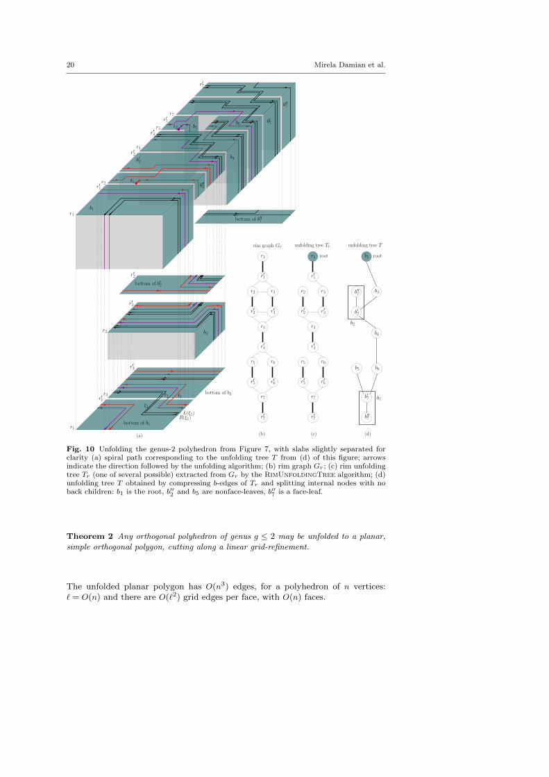
Figure 10 shows the complete spiral path for the genus-2 polyhedron from Fig-ure 7, with the slabs slightly separated for clarity. In this example ` = 1, ξ1corresponds to node b′′7 with back face-rim r′7, and the t1 and t2 paths correspondto b′′2 and b5, with back nonface-rims r2 and r5, respectively. (For clarity, the pathst1 and t2 are labeled on the bottom face of b3, as they make the transition to thebottom face of b1.)
3.3 Level of Refinement
Using the Chang-Yen algorithm [CY15], any genus-0 orthogonal polyhedron P canbe unfolded using linear refinement. Specifically, they refine each rectangular faceof P via grid-unfolding using a (2` × 4`)-grid, where ` is the number of leavesin T , and cuts are allowed along any of these grid lines. In the worst case, thealgorithm presented here requires at most twice the level of refinement, i.e., (4`×8`)refinement. This level of refinement is necessary when there are two nonface-leavesin T . In this case, the first part of the spiral path (from L(ξ1) to the end of t1located on the back rim of the first nonface-leaf is the same as in the Chang-Yenalgorithm, but with care given to the order in which the spiral paths are connectedand with only one endpoint of t1 at the root. (This is the black and blue portionsof the path illustrated in Figure 9.) Thus no additional refinement is necessaryfor this part of the path. The doubling of the refinement is due to the retracingof this path which is needed to extend it from L(ξ1) to t2, the spiral path of thesecond nonface-leaf. (This is the red portion of the path in Figure 9.) Becausethe retracing follows alongside the existing path, it requires twice the refinement.Thus, the overall level of refinement is (4`× 8`), which is linear.
We conclude with this theorem:
20 Mirela Damian et al.
r1
r′1
r2 r3
r′2 r′3
r4
r′4
r5 r6
r′5 r′6
r7
r′7
r1
r′1
r2 r3
r′2 r′3
r4
r′4
r5 r6
r′5 r′6
r7
r′7
unfolding tree Trrim graph Gr
r1
r′1r2
r′2r4
r′4r5
r′5r7
r′7
r′2
r3
r′3
r1
r′1r3
r′3
b1
b′2b4
b5b6
bottom of b′2
b3
bottom of b3
bottom of b1
(a) (b) (c)
t2
root
t1t2
ξ1
R(ξ1)L(ξ1)
b1
b′′2 b3
b′2
b4
b5 b6
b′7
b′′7
unfolding tree T
(d)
root
b2
b7
t1
b′′7
b′7
b′′2
bottom of b′′7
Fig. 10 Unfolding the genus-2 polyhedron from Figure 7, with slabs slightly separated forclarity (a) spiral path corresponding to the unfolding tree T from (d) of this figure; arrowsindicate the direction followed by the unfolding algorithm; (b) rim graph Gr; (c) rim unfoldingtree Tr (one of several possible) extracted from Gr by the RimUnfoldingTree algorithm; (d)unfolding tree T obtained by compressing b-edges of Tr and splitting internal nodes with noback children: b1 is the root, b′′2 and b5 are nonface-leaves, b′′7 is a face-leaf.
Theorem 2 Any orthogonal polyhedron of genus g ≤ 2 may be unfolded to a planar,
simple orthogonal polygon, cutting along a linear grid-refinement.
The unfolded planar polygon has O(n3) edges, for a polyhedron of n vertices:` = O(n) and there are O(`2) grid edges per face, with O(n) faces.
Unfolding Genus-2 Orthogonal Polyhedra with Linear Refinement 21
4 Conclusion
It is not evident how to push the techniques common to [DFO07], [DDF14], and[CY15] to unfold polyhedra of genus g ≥ 3, the next frontier in this line of research.Both Lemma 1 (existence of a face-node to serve as root of T ) and Theorem 1 (theRimUnfoldingTree algorithm leads to at most g ≤ 2 nonface-leaves) are crucialin the unfolding algorithm described in Section 3. The final stitching together ofthe spiral paths relies on there being at most two nonface-leaves of the unfoldingtree T .
On the other hand, it is not difficult to unfold the genus-3 polyhedron shownin Figure 6b in an ad-hoc manner. The challenge is to find a generic algorithm forgenus-3 and beyond.
Acknowledgement. We thank all the participants of the 31st Bellairs WinterWorkshop on Computational Geometry for a fruitful and collaborative environ-ment. In particular, we thank Sebastian Morr for important discussions relatedto Theorem 1, and to the stitching of unfolding strips at the root node.
References
BDD+98. Therese Biedl, Erik Demaine, Martin Demaine, Anna Lubiw, Mark Overmars,Joseph O’Rourke, Steve Robbins, and Sue Whitesides. Unfolding some classes oforthogonal polyhedra. In Proceedings of the 10th Canadian Conference on Com-putational Geometry, Montreal, Canada, August 1998.
BDE+03. Marshall Bern, Erik D. Demaine, David Eppstein, Eric Kuo, Andrea Mantler, andJack Snoeyink. Ununfoldable polyhedra with convex faces. Computational Geom-etry: Theory and Applications, 24(2):51–62, February 2003.
CY15. Yi-Jun Chang and Hsu-Chun Yen. Unfolding orthogonal polyhedra with linearrefinement. In Proceedings of the 26th International Symposium on Algorithmsand Computation, ISAAC 2015, Nagoya, Japan, pages 415–425. Springer BerlinHeidelberg, 2015.
DDF14. Mirela Damian, Erik D. Demaine, and Robin Flatland. Unfolding orthogonal poly-hedra with quadratic refinement: the delta-unfolding algorithm. Graphs and Com-binatorics, 30(1):125–140, 2014.
DFMO05. Mirela Damian, Robin Flatland, Henk Meijer, and Joseph O’Rourke. Unfoldingwell-separated orthotrees. In Abstracts from the 15th Annual Fall Workshop onComputational Geometry, Philadelphia, PA, November 2005.
DFO07. Mirela Damian, Robin Flatland, and Joseph O’Rourke. Epsilon-unfolding orthog-onal polyhedra. Graphs and Combinatorics, 23(1):179–194, 2007.
DFO08. Mirela Damian, Robin Flatland, and Joseph O’Rourke. Unfolding Manhattan tow-ers. Computational Geometry: Theory and Applications, 40:102–114, 2008.
DM04. Mirela Damian and Henk Meijer. Edge-unfolding orthostacks with orthogonallyconvex slabs. In Abstracts from the 14th Annual Fall Workshop on ComputationalGeometry, pages 20–21, Cambridge, MA, November 2004. http://cgw2004.csail.mit.edu/talks/34.ps.
DO07. Erik D. Demaine and Joseph O’Rourke. Geometric Folding Algorithms: Linkages,Origami, Polyhedra. Cambridge University Press, July 2007.
LPW14. Meng-Huan Liou, Sheung-Hung Poon, and Yu-Jie Wei. On edge-unfolding one-layer lattice polyhedra with cubic holes. In The 20th International Computing andCombinatorics Conference (COCOON) 2014, pages 251–262, 2014.


![Edge-Compositions of 3D Surfaces · compositions of unfoldings is related to that of edge-unfolding of polyhedra from the field of computational geometry (See Ref. [10] for a survey](https://static.fdocuments.us/doc/165x107/5fcb196935e05d4b4c3e962a/edge-compositions-of-3d-surfaces-compositions-of-unfoldings-is-related-to-that-of.jpg)