FEDERAL RESERVE BANK OF SAN FRANCISCO

WORKING PAPER SERIES

Working Paper 2009-04 http://www.frbsf.org/publications/economics/papers/2009/wp09-04bk.pdf

The views in this paper are solely the responsibility of the authors and should not be interpreted as reflecting the views of the Federal Reserve Bank of San Francisco or the Board of Governors of the Federal Reserve System.

Unemployment Dynamics in the OECD

Michael Elsby University of Edinburgh and NBER

Bart Hobijn

FRB San Francisco

Aysegül Sahin FRB New York

February 2011

Unemployment Dynamics in the OECD�

Michael W. L. Elsby

University of Edinburgh and NBER

Bart Hobijn

FRB San Francisco

Aysegül Sahin

FRB New York

February 2011

Abstract

We provide a set of comparable estimates for the rates of in�ow to and out�ow from

unemployment using publicly available data for fourteen OECD economies. We then

devise a method to decompose changes in unemployment into contributions accounted

for by changes in in�ow and out�ow rates for cases where unemployment deviates from

its �ow steady state, as it does in many countries. Our decomposition reveals that

�uctuations in both in�ow and out�ow rates contribute substantially to unemployment

variation within countries. For Anglo-Saxon economies we �nd approximately a 15:85

in�ow/out�ow split to unemployment variation, while for Continental European and

Nordic countries, we observe much closer to a 45:55 split. Using the estimated �ow

rates we compute gross worker �ows into and out of unemployment. In all economies

we observe that increases in in�ows lead increases in unemployment, whereas out�ows

lag a ramp up in unemployment.

Keywords: Unemployment, Worker �ows, Job Finding Rate, Separation Rate.

JEL-codes: E24, J6.

�We would like to thank anonymous referees, Regis Barnichon, Shigeru Fujita, Wilbert van der Klaauw,Emi Nakamura, Simon Potter, Gary Solon, participants at the New York/Philadelphia Workshop on Quan-titative Macroeconomics 2008, Midwest Macroeconomics Conference 2009, Recent Developments in Macro-economics Conference 2009, EEA Conference 2009, CREI/Kiel Conference on Macroeconomic Fluctuationsand the Labor Market 2009 for helpful comments, and Joseph Song for outstanding research assistance. Theviews expressed in this paper are those of the authors and do not necessarily re�ect those of the Federal Re-serve Bank of New York, the Federal Reserve Bank of San Francisco or the Federal Reserve System. An Excelspreadsheet with all the data, calculations, and results presented in this paper is available for download athttp://www.frbsf.org/economics/economists/bhobijn/UnemploymentDynamicsInTheOECD.xlsm. Thanksto Jonas Staghøj for pointing out a coding error in a previous version of the spreadsheet. E-mail addressesfor correspondence: mike.elsby@ed.ac.uk; bart.hobijn@sf.frb.org; aysegul.sahin@ny.frb.org.

1

1 Introduction

Unemployment rates among developed economies have varied substantially both across time

and across countries over the last 40 years. This variation in unemployment may occur as a

result of variation in the rate at which workers �ow into the unemployment pool, variation

in the rate at which unemployed workers exit the unemployment pool, or a combination

of the two. The relative contributions of changes in in�ow and out�ow rates to changes

in unemployment have been abundantly documented for the U.S.1 Less is known, however,

about the driving forces of unemployment variation in other countries. Such a question is

of interest because of the considerable variation in unemployment that has been observed

in developed economies in recent decades, notably in Continental Europe. In this paper, we

provide a detailed analysis of unemployment �ows for fourteen developed economies using

publicly available data.

In the �rst part of our analysis we describe how it is possible to derive measures of the

rates of in�ow2 to and out�ow from the unemployment pool using annual data from the

OECD. To do this, we generalize the method developed by Shimer (2007), which makes use

of time series for the number employed, the number unemployed, and the number unem-

ployed less than �ve weeks to infer �ow hazard rates for the U.S. A limitation that arises

when applying this methodology outside the U.S. is that series on short duration unemploy-

ment can be noisy for countries in which short durations account for a small proportion

of overall unemployment, such as in Continental Europe. To address this, we develop a

method that exploits additional data on unemployment at higher durations to construct a

set of comparable time series for the unemployment in�ow and out�ow rates across countries.

Our measures allow us to document a set of stylized facts on unemployment �ows among

developed economies. First, the average level of unemployment in�ow and out�ow rates

varies substantially across countries. Interestingly, the results suggest a natural partition-

ing of economies into Anglo-Saxon, Nordic and Continental European. Anglo-Saxon and

Nordic economies display high exit rates from unemployment, with monthly hazards that

exceed 20 percent. In stark contrast, out�ow rates among Continental European economies

1See Elsby, Michaels, and Solon [2009], Fujita and Ramey [2008], Hall [2005a,b], Shimer [2007], andYashiv [2007].

2Some recent literature on unemployment �ows has referred to the rate of in�ow into unemployment asthe �separation rate� (Shimer, 2005a, b; Fujita and Ramey, 2008). We refer to it as the in�ow rate fortwo reasons. First, a separation is typically taken to mean a quit or a layo¤ from an employer. In thepresence of job-to-job transitions, such separations need not lead to an unemployment spell. Second, someunemployment spells originate from non-participation rather than a separation from employment.

2

are much lower� typically less than 10 percent at a monthly frequency. Symmetrically, un-

employment in�ow rates also vary considerably across countries. Anglo-Saxon and Nordic

countries exhibit in�ow hazards that exceed 1.5 percent at a monthly frequency. However, as

with the observed levels of out�ow rates, monthly in�ow rates among Continental European

economies are again much lower at around 0.5 to 1 percent. These observations con�rm the

diagnosis that European labor markets are sclerotic in the sense that they display much lower

rates of reallocation of labor, as documented in Blanchard and Summers (1986), Bertola and

Rogerson (1997), Blanchard and Wolfers (2000), and Blanchard and Portugal (2001).

In the second part of our analysis, we pose the question of how much of the observed vari-

ation in unemployment within each country can be accounted for by variation in the in�ow

rate into unemployment and variation in the out�ow rate from unemployment respectively.

To answer this, we provide a method for decomposing changes in the unemployment rate

into contributions due to changes in the �ow hazards that can be applied in countries with

very di¤erent unemployment dynamics. Recent literature (Elsby, Michaels, and Solon [2009],

Fujita and Ramey [2009], Petrongolo and Pissarides [2008]) has evaluated these contributions

under the assumption that the unemployment rate is closely approximated by its �ow steady

state value. Under this assumption, contemporaneous unemployment variation may be de-

composed into contributions related to contemporaneous logarithmic variation in in�ow and

out�ow hazards. While this steady state assumption holds as a reasonable approximation

in the U.S., we show that it can be very inaccurate in other developed economies, notably

those of Continental Europe.

Reacting to this we show that, in cases where unemployment deviates from steady state,

current variation in unemployment can be decomposed recursively into contributions due

to current and past logarithmic changes in the in�ow and out�ow hazards. Intuitively,

when unemployment is out of steady state, it can vary as a result of contemporaneous

changes in the in�ow and out�ow rates, or as a result of dynamics driven by past changes in

these �ow hazards. Using our alternative decomposition, we obtain a much more accurate

characterization of changes in unemployment rates across countries.

Application of our decomposition to our estimated time series for the �ow hazard rates

provides us with a second stylized fact on unemployment �ows. Among all countries that we

consider, �uctuations in both in�ow and out�ow rates contribute substantially to unemploy-

ment variations within countries. The relative contribution of each di¤ers across countries,

however. Among Anglo-Saxon economies we �nd approximately a 15:85 in�ow/out�ow split

of unemployment variation, a result that echoes recent �ndings for the U.S. over the same

3

sample period. For Continental European and Nordic countries, however, we observe much

closer to a 45:55 in�ow/out�ow split. Thus, a complete understanding of unemployment

variation among our large sample of developed economies requires an understanding of the

determinants of both the in�ow rate as well as the out�ow rate.

The �nal part of our empirical analysis uses the estimated �ow hazard rates to compute

measures of the number of workers �owing in and out of the unemployment pool (as opposed

to the hazard rates for these �ows).3 A third stylized fact that emerges from these results is

that a geographical partitioning also applies to average worker �ows across countries. Anglo-

Saxon and Nordic countries exhibit annual worker �ows in and out of unemployment that

comprise more than 15 percent of the labor force. Among Continental European economies,

on the other hand, worker �ows typically involve less than 10 percent of the labor force,

echoing the �ndings of Blanchard and Portugal (2001) and Bertola and Rogerson (1997).

We then analyze the dynamic relationship between these worker �ows and unemployment

within each country. Using a simple correlation analysis, we document a fourth stylized fact

on unemployment �ows among developed economies: The timing of the contributions of

in�ows and out�ows to unemployment variation displays a remarkable uniformity across

countries. In all economies we observe that increases in in�ows lead increases in unem-

ployment, whereas out�ows lag a ramp up in unemployment, an observation that has been

highlighted for the U.S. in earlier studies.4

Our �ndings that variation in unemployment in�ows accounts for a substantial fraction of

unemployment variation and is an important leading indicator for changes in unemployment

dovetails with a recent literature on U.S. unemployment �ows. A growing trend in modern

macroeconomic models of the aggregate labor market has been to assume that the in�ow rate

into unemployment is acyclical (Hall [2005a,b], Shimer [2005] among others). Reacting to

this, a number of recent studies has cautioned against this trend by documenting evidence for

systematic countercyclical movements in unemployment in�ows in U.S. data.5 Our �ndings

3Our analysis is not the �rst to estimate worker �ows across countries. Other studies that examine worker�ows for a subset of European countries include Albaek and Sørensen (1998) for Denmark; Bauer and Bender(2004) and Bachmann (2005) for Germany; Bertola and Rogerson (1997) for Canada, Germany, Italy, theU.K., and the U.S.; Burda and Wyplosz (1994) for France, Germany, Spain, and the U.K.; Petrongolo andPissarides (2008) for France, Spain and the U.K.; and Pissarides (1986), Bell and Smith (2002), and Gomes(2008) for the U.K. Reichling (2005) reports estimates of the separation rate for a set of countries (see hisTable 5) and also emphasizes that the separation rate is lower in European countries than in the U.S.

4See Darby, Haltiwanger, and Plant [1985, 1986], Blanchard and Diamond [1990], Davis [2006], Fujitaand Ramey [2008].

5Recent studies that have emphasized this fact include Braun, De Bock, and DiCecio (2006); Davis (2006);Elsby, Michaels, and Solon (2009); Fujita and Ramey (2008); Kennan (2006); and Yashiv (2008). Older

4

show that this caution resonates all the more if we wish to understand the considerable

variation in unemployment rates observed outside the U.S.

The remainder of the paper is organized as follows. In section 2 we summarize the OECD

data that we use throughout our analysis. In section 3, we describe our methodology for

inferring the rates of in�ow to and out�ow from the unemployment pool using the OECD

data. Application of this methodology provides individual time series for the unemployment

�ow hazards for each of the fourteen countries in our sample. In section 4, we pose the

question of how much of the variation in unemployment within countries can be accounted

for by changes in the in�ow and out�ow rates respectively. To answer this question, we

derive a decomposition of unemployment variation that allows for unemployment to deviate

from steady state. We show that allowing for such deviations is critical for understanding

unemployment �uctuations outside the U.S. Section 5 presents evidence on the number of

workers �owing in and out of unemployment, and documents stylized facts on the timing

of the impact of worker �ows on unemployment changes. Section 6 summarizes and o¤ers

conclusions.

2 Data

Since a large part of our analysis is informed by the available data, we start by discussing

the OECD samples that we use. These are taken from two di¤erent sources. First, we

use annual measures of the unemployment stock by duration, taken from OECD (2010a).6

We then supplement these data with quarterly measures of the aggregate unemployment

rate, taken from OECD (2010b). Both slices of data are based on the labor force surveys

conducted in each of the countries in our sample.

The fourteen economies that we focus on are: Australia, Canada, France, Germany,

Ireland, Italy, Japan, New Zealand, Norway, Portugal, Spain, Sweden, United Kingdom,

and the United States. For all countries relatively long historical quarterly time series are

available for the unemployment rate. Our focus on these economies is primarily driven by

the length of the available requisite series for unemployment by duration. Throughout, we

denote the fraction of the labor force in an unemployment spell of less than d months in

month t by u<dt .7 For our analysis we use annual time series for u<1t , u

<3t , u

<6t , and u

<12t .

studies that have documented this include Perry (1972); Marston (1976); Blanchard and Diamond (1990);and Baker (1992).

6The data are also publicly available on the web from http://stats.oecd.org.7For many countries, data on unemployment duration initially were collected only once a year. More

5

Note that we de�ne these categories inclusively, in the sense that u<3t includes u<1t , and so

on. The starting year for the available series varies between 1968 (for the U.S.) and 1986

(for New Zealand and Portugal).8 For all countries, the data end in 2009.

An important advantage of using data from the OECD is that, even though the labor force

surveys of these countries have di¤erent structures, the OECD data have been standardized

to adhere to the same structure. This aids cross-country comparisons of our results.9

3 The Ins and Outs of Unemployment in the OECD

At the heart of our analysis is a set of estimated annual time series of �ow hazard rates into

and out of unemployment for fourteen OECD countries. These time series are estimated using

an extension of the method that Shimer (2007) developed for the United States. Shimer�s

method cannot be applied directly to other OECD countries because the required data are

not available. The extension that we introduce allows us to overcome this limitation and to

produce annual time series for the rates of in�ow to and out�ow from the unemployment

pool for a large subset of OECD countries.

3.1 Analytical Framework

The evolution over time of the unemployment rate, which we denote by ut, can be written

as:10dutdt= st(1� ut)� ftut; (1)

where st is the monthly rate of in�ow into unemployment, ft is the monthly out�ow rate

from unemployment, and t indexes months.11 As mentioned above, the data that we use in

recently, mainly due to the standardization of Labor Force Surveys in the European Union, countries arecollecting these data at a quarterly frequency. Because our aim is to construct historical time series that areas long as possible, we focus on annual time series.

8The initial year in the sample for each country is listed in Table 2.9While the OECD goes to some lengths to standardize their unemployment measures, their procedures

may not be perfect. For example, it is possible that workers who de�ne themselves as out of the labor forcein e.g. the U.S. might de�ne themselves as unemployed in Europe. Addressing these important issues ofstandardization is beyond the scope of this paper.10It is important to note that equation (1) implicitly assumes that all of the in�ow into unemployment

originates from employment. We have calculated a set of results taking into account non-participation.Except for the level of the average in�ow rate, these results were very similar to those we present here.Details of these results, as well as an explanation of why this is the case are provided in the Appendix.11We de�ne the �ow hazards st and ft in monthly terms to aid comparison with estimates reported in

U.S. studies of unemployment �ows.

6

the remainder of the paper allow us to infer unemployment �ows at an annual frequency.

Thus, we would like to relate the continuous time evolution of unemployment in equation (1)

to the unemployment rates that we observe at discrete annual intervals. Assuming that the

�ow hazards are constant within years,12 and solving equation (1) forward one year allows

us to do this:

ut = �tu�t + (1� �t)ut�12, (2)

where

u�t =st

st + ft(3)

denotes the �ow steady-state unemployment rate, and

�t = 1� e�12(st+ft) (4)

is the annual rate of convergence to steady state. In this way we can relate variation in

the unemployment stock ut in a given country over the course of a year to variation in

the underlying �ow hazards, st and ft.13 To implement this, however, we need to obtain

estimates of these �ow hazards, to which we now turn.

Our method for estimating the out�ow rate ft is an extension of the method popularized

by Shimer (2007). In his study of U.S. unemployment �ows, he infers the monthly out�ow

probability Ft using the identity that the monthly change in the unemployment stock is given

by

ut+1 � ut = u<1t+1 � Ftut. (5)

Here u<1t+1 denotes the stock of unemployed workers with duration less than one month, and

hence re�ects the �ows into unemployment; Ftut re�ects the �ows out of unemployment.

12This assumption does lead to some smoothing out of high frequency variation in the �ow hazards thatwe estimate. As many U.S. studies of unemployment �ows have shown, and as we will con�rm in our cross�country estimates, it is predominantly the in�ow rate st that displays such high frequency variation. Itfollows that annual smoothing is likely to lead to an overstatement of the contribution of changes in theout�ow rate ft to unemployment variation. This works against a key �nding of this paper that variation inthe in�ow rate st accounts for a substantial fraction of unemployment variation.13For simplicity, we abstract from labor force growth in equations (1) through (4). It is straightforward

to show, however, that if the labor force grows at monthly rate gt, then u�t = st=(st + ft + gt) and �t =1�e�12(st+ft+gt). In our sample, gt averages around 0.001 on a monthly basis. In contrast, the average valueof (st + ft) in our sample is on the order of 0.2. This point also extends to speci�c countries and periods inwhich labor force growth accelerates. For example, gt rose in the 2000s in Spain up to 0.003 on a monthlybasis. However, over the same period, we observe that (st+ ft) averages around 0.1 in Spain. Consequently,allowing for labor force growth does not a¤ect our results in a quantitatively important way.

7

Solving for the monthly out�ow probability, one obtains14

Ft = 1�ut+1 � u<1t+1

ut. (6)

The monthly out�ow probability is then related to the associated monthly out�ow hazard

rate, f<1t , through

f<1t = � ln(1� Ft). (7)

3.2 Estimation of Flow Hazard Rates

Duration Dependence and Estimation of the Out�ow Rate In what follows we will

see that the estimate of the out�ow rate implied by equation (6) works well for countries

in which the out�ow rate from unemployment is relatively high, such as the U.S. However,

in countries that exhibit low exit rates, such as those of Continental Europe, estimates

based on equation (6) can be substantially noisy. The simple reason is that low out�ow

rates imply that very few unemployed workers at a point in time are in their �rst month of

unemployment, which increases the sampling variance of the estimate of u<1t+1, and in turn

leads to noisy estimates of ft.15

Our approach to this problem is to use the additional unemployment duration data

available from the OECD to increase the precision of our estimate of ft in countries where

the out�ow rate is low. To see how this may be done recall that the OECD data also report

the unemployment stock at durations higher than one month. It follows that, analogous to

the method detailed above, it is possible to write the probability that an unemployed worker

14Since the OECD database reports only quarterly data on the aggregate unemployment rate, we computeut by interpolating quarterly data.15For example, the OECD data for the U.S. are based on the Current Population Survey, which surveys

around 130,000 individuals each month. In the U.S., the labor force participation rate averaged 47.9 percent,6.1 percent of which were unemployed, 43.3 percent of which were unemployed for less than one month. Thissuggests around 130; 000� 0:479� 0:061� 0:433 � 1; 645 respondents have been unemployed less than onemonth in each month�s survey. In contrast, each survey for Germany includes around 165,000 respondents,with an average participation rate of 48.5 percent, 8.3 percent of which were unemployed, but only 6.9percent of which were unemployed for less than one month. This implies that only around 458 respondentshave been unemployed for less than one month in each survey for Germany. This simple comparison wouldsuggest that the sampling variance of the estimate of short-term unemployment in each survey in Germanywill be 3.6 times its U.S. equivalent. In addition, this calculation becomes much more extreme when oneaccounts for the fact that the OECD data for the U.S. are annual averages of monthly data, while thosefor Germany correspond to just one month, April. Similar calculations for other European countries yieldsimilar conclusions.

8

exits unemployment within d months as

F<dt = 1�ut+d � u<dt+d

ut. (8)

As before, this can be mapped into an out�ow rate estimate given by

f<dt = � ln(1� F<dt )=d: (9)

Given the available data, we can estimate f<dt for d = 1; 3; 6; 12.16

It is important to clarify the interpretation of the out�ow rate measures f<dt . It is

tempting to interpret f<dt as the out�ow rate for unemployed workers of duration d. However,

that is not an accurate interpretation. Rather, it is the hazard rate associated with the

probability that an unemployed worker at time t completes her spell within the subsequent

d months.

These four measures, f<1t ; f<3t ; f

<6t ; and f

<12t , are not necessarily estimates of the same

out�ow rate. Only in the case where the out�ow hazard is unrelated to the duration of an

unemployment spell, i.e. if there is no duration dependence in out�ow rates, are all four

measures consistent estimates of the aggregate out�ow rate from unemployment, de�ned

as the average out�ow rate among the entire unemployed population. However, if there is

duration dependence in unemployment out�ow rates in a given country, then estimates based

on durations of unemployment greater than one month, f<3t ; f<6t ; and f

<12t , will not yield

consistent estimates of the average out�ow rate among the unemployed.

For example, imagine that there exists negative duration dependence whereby the out�ow

rate declines with duration.17 In such an environment, we would expect to observe f<1t >

f<3t > f<6t > f<12t . To see why, consider the version of equation (8) which expresses the

fraction of the unemployment stock in month t that exits within the next three months.

The remaining unemployed workers that do not exit over these subsequent three months

increasingly will be comprised of unemployed workers with low out�ow rates, i.e. the high

duration unemployed. This process of dynamic selection will imply that excessive weight

will be placed on the low out�ow rates of high duration unemployed workers in the estimate

of f<3t , generating a downward bias in its estimate of ft. This argument applies even more

16The appendix contains a detailed description on how we estimate these rates combining the annual andquarterly data available.17In the U.S., for example, the �nding of substantial negative duration dependence in unemployment exit

rates has been widely documented since Kaitz (1970). Most recently, Shimer (2008) has emphasized thisstylized fact for the U.S.

9

strongly to the estimates of f<6t and f<12t .18

In light of this, we formally test for the presence of duration dependence in out�ow rates

by testing the hypothesis that f<1t = f<3t = f<6t = f<12t . The formal details are described

in the Appendix, but our general approach is as follows. First, we derive the asymptotic

distribution of the unemployment rates by duration as well as for the unemployment rates.

We then apply the Delta method to compute the joint asymptotic distribution of the out�ow

rate estimates f<dt with d = 1; 3; 6; 12. This allows us to formulate a simple Chi-squared test

of the null hypothesis of no duration dependence.

It should be noted that we test for a very broad de�nition of duration dependence.

As has been emphasized since Kaitz (1970), duration dependence can arise through two

channels. �True�duration dependence refers to the case where unemployment duration has

a causal e¤ect on the out�ow rates of individual workers. In contrast, �spurious�duration

dependence refers to the process of dynamic selection whereby workers with high exit rates

leave unemployment faster than those with low exit rates, thereby generating a negative

correlation between duration and out�ow rates (Salant, 1977). Our hypothesis test is not

intended to distinguish between these two sources of duration dependence, but rather to

test for whether the alternative measures of the out�ow rate derived above are signi�cantly

di¤erent from one another. Thus, the duration dependence we test for can arise due to either

dynamic selection or true duration dependence or both.

For those countries for which we reject the hypothesis of no duration dependence, we

follow the recent U.S. literature in using f<1t as our estimate of the unemployment out�ow

rate, as this measure provides the most accurate estimate of the average out�ow rate in the

presence of duration dependence. For countries with weak evidence for duration dependence

for which we do not reject the null, we make use of all the additional information on the

out�ow rate contained in f<3t ; f<6t ; and f

<12t in order to obtain a more precise estimate of ft.

Speci�cally, we use our estimates of the asymptotic distribution of the out�ow rate estimates,

f<1t ; f<3t ; f

<6t ; and f

<12t to compute an optimally weighted estimate of the out�ow rate that

minimizes the mean squared error of the estimate.19

The results of the hypothesis test are reported in Table 2. While we �nd signi�cant

evidence of duration dependence in Anglo-Saxon and Nordic countries and Japan, we do not

observe signi�cant evidence among the Continental European countries in our sample.20 It is

18By the same token, the estimate of f<1t that has been widely used in recent literature is also subject tothis drawback, just to a lesser degree than the other three measures.19The construction of these optimal weights is detailed in the Appendix.20While our hypothesis test provides a natural rule of thumb, we implicitly rule in favor of the null when

10

natural to ask whether this conclusion is supported by the results of microeconometric studies

that estimate duration dependence for speci�c European economies. A particularly useful

summary of this literature is reported by Machin and Manning (1999, Table 6). They show

that the evidence for duration dependence among European economies is quite inconclusive.

Estimates of duration dependence in Germany and Spain, for example, di¤er across studies,

with evidence found for negative, positive and negligible duration dependence reported. Our

conclusion of limited evidence for duration dependence lies at the midpoint of this array.

A clearer consensus emerges for France and the U.K. For France, the literature �nds very

little evidence for duration dependence, at least within the �rst year of the unemployment

spell. In contrast, for the U.K., the literature in general �nds evidence for negative duration

dependence. Our estimates are in line with these conclusions.

Our results are also consistent with other work that has estimated duration dependence

across countries. In their own analysis, Machin and Manning (1999) �t a Weibull dura-

tion model to the duration structure of unemployment across countries. They report weak

negative duration dependence in France and Spain in the 1990s, but strong negative du-

ration dependence in Australia, the U.K. and the U.S. in the 1980s and 1990s. Using a

similar approach on OECD data, Hobijn and Sahin (2009) also �nd little evidence of dura-

tion dependence among Continental European economies, but substantial evidence among

economies with high unemployment out�ow rates. The result of our hypothesis test is that

we use f<1t as our estimate of the out�ow rate for the Anglo-Saxon countries in our sample

and the optimally weighted average of f<1t ; f<3t ; f

<6t ; and f

<12t for the remaining countries.

Temporal Aggregation Bias and Estimation of the In�ow Rate Given our estimate

of the out�ow rate, we compute the in�ow rate st using the method pioneered by Shimer

(2007). In particular, note that the expression for the annual unemployment rate in equation

(2) is simply a nonlinear equation in the unemployment rates, ut+12 and ut, and the �ow

hazard rates, st and ft. We can thus solve equation (2) for the in�ow rate.

As emphasized by Shimer (2007) and subsequent work based on his method, this estimate

of the in�ow rate is robust to temporal aggregation bias in the measurement of unemployment

in�ows. In particular, since equation (2) is inferred from solving forward the continuous-time

di¤erential equation for the evolution of the unemployment rate, it accounts for the fact that

the hypothesis of no duration dependence cannot be rejected. This raises the question of the power of thetest. In results that can be replicated in the spreadsheet that accompanies this paper, we observe that thetest does indeed have high power among the Continental European economies for which we fail to reject thenull, in the sense that the estimates of f <dt are similar for all durations d.

11

workers who �ow into unemployment after one period�s survey may exit prior to the next

period�s survey, �ows that would be missed in discrete-time data. Correcting for temporal

aggregation bias in the in�ow rate is particularly important the context of the OECD data,

since the data are available at an annual frequency, in contrast to the monthly data that are

available for the U.S.21

A natural question is whether a symmetric bias a¤ects estimation of the out�ow rate.

Interestingly, time aggregation causes relatively little bias in the out�ow rate, for two reasons.

First, consider the measure of the out�ow probability in equation (6). This is just the

complement of the probability that those unemployed at time t remain unemployed by time

t + 1. If there were a time aggregation problem, the concern would be that the data fail to

pick up on workers who exit unemployment after one period�s survey, but who re-enter prior

to the next period�s survey. However, the measure of the out�ow probability in equation (6)

does not miss such transitions: Any worker who followed this path would be identi�ed as

short-term unemployed in the second survey, and therefore correctly counted as an out�ow.

Second, it still could be the case that the measure of the out�ow probability in equation (6)

misses multiple exits from unemployment within the period (e.g. out after �rst survey, in

again, out again, in again prior to next survey). However, we will see that the in�ow rate in

practice is very small in comparison to the out�ow rate for all countries in our sample, so

that the probability of such multiple transitions is likely to be miniscule.22

3.3 Evidence from OECD Data

The average unemployment in�ow and out�ow hazards over the sample periods for the whole

sample of countries are reported in Table 2. A striking observation from these results is the

substantial cross-country variation in both st and ft. A particularly useful illustration of

this point is in Figure 1, which displays the average values of st and ft from Table 2 in graph

form. Interestingly, one can discern a natural partition of developed economies between

Anglo-Saxon, Nordic and Continental European economies.

Figure 1 reveals very high out�ow rates among the Anglo-Saxon and Nordic economies.

21The magnitude of the correction for time aggregation bias in in�ow rates also will vary across countries. InEuropean economies with sclerotic unemployment �ows, we will see that the out�ow rate from unemploymentft is low. As a result, the correction for time aggregation bias is smaller for these countries, as a lowerproportion of in�ows into unemployment after one survey will exit unemployment prior to the next survey.22Shimer (2007) makes a similar point. In his words: �Because the probability of losing a job during the

month that it is found is comparatively small, time aggregation causes relatively little bias in the job �ndingrate.�

12

Among these countries the average monthly unemployment out�ow hazard exceeds 20 per-

cent. The economies of Continental Europe stand in stark contrast. Unemployment out�ow

rates in these economies lie below 10 percent at a monthly frequency. A similar picture

develops for the estimates of the in�ow rates in Figure 1. We observe high unemployment

in�ow hazards among the Anglo-Saxon and Nordic economies, which typically lie above 1.5

percent on a monthly basis. Likewise, in�ow rates among the European economies are again

much lower at around 0.5 to 1 percent per month.

Figure 1 also shows that there are both extremes and intermediate cases that are un-

derstated in this Anglo-Saxon/Nordic/Continental Europe taxonomy. For Japan, while the

average unemployment out�ow rate of 19 percent is similar to those in Anglo-Saxon and

Nordic economies, its in�ow rate is more comparable to those of Continental Europe. An-

other intermediate case is the U.K., which displays unemployment �ows that lie halfway

between the Anglo-Saxon and the Continental European models. Perhaps the most striking

observation, however, is the outlier status of the U.S. With an average monthly unemploy-

ment out�ow rate of nearly 60 percent and an average in�ow rate of 3.5 percent, it exhibits

transition rates at least 50 percent larger than the remainder of our sample of countries.

Figures 2 and 3 display the time series for the in�ow and out�ow hazards for each country

in our sample. The transition rates are plotted on log scales since, as emphasized in the

literature on unemployment �ows, and as we will con�rm in what follows, it is the logarithmic

variation in st and ft that places them on an equal footing with respect to �uctuations in

the unemployment rate.

Figures 2 and 3 reveal that, in addition to signi�cant cross-country variation in unem-

ployment �ows, there is also substantial variation in unemployment �ow hazards over time

within countries. Although there is a great deal of information contained in these �gures,

a number of observations come to light. First, there are important di¤erences in the fre-

quency of �uctuations in unemployment �ows across economies. Among the Anglo-Saxon

economies, a clear cyclical pattern is present, suggesting a substantial high frequency com-

ponent to unemployment �uctuations in these countries. Among other economies, however,

the variation in st and ft occurs at a much lower frequency, and it is hard to di¤erentiate

cycle from trend.

Figures 2 and 3 are also indicative of how the relative contributions of variation in the

in�ow and out�ow rates di¤er across countries. Speci�cally, the Anglo-Saxon economies

appear to display relatively more variation in the out�ow rate from unemployment, a point

that has been emphasized in recent literature for the U.S. However, inspection of the time

13

series for the Nordic and European economies reveals greater variation in the in�ow rate,

suggesting about an equal contribution of the ins and the outs to unemployment variation

in these countries.

Figures 2 and 3 also provide a sense of the degree to which these stylized facts have held

true in the most recent recession. In many respects, historical di¤erences in unemployment

dynamics between Anglo-Saxon and Continental European economies have been echoed in

recent data. Inspection of the time series for the �ow hazards after 2007 reveals that, as in the

past, the recent rise in unemployment has been associated more with rises in unemployment

in�ows in Continental European economies, and with declines in rates of out�ow in Anglo-

Saxon countries. Figures 2 and 3 do point to one stark feature of the recession, however:

The out�ow rate from unemployment in the U.S. fell precipitously to reach a historic low,

a point noted by many observers of the Great Recession in the U.S. (see Elsby, Hobijn and

Sahin [2010], for example). An advantage of the cross-country estimates in Figures 2 and 3

is that they provide a useful perspective on this phenomenon. Despite the record decline in

rates of exit from unemployment in the U.S., the level of the out�ow rate witnessed recently

in the U.S. still dwarfs those observed in Continental Europe.

Of course, this visual impression is only suggestive of the relative contributions of the

in�ow and out�ow hazards to unemployment variation; we address this issue more formally

in section 4. Before we do so, we �rst compare our estimates of unemployment transition

rates with those reported in related literature.

3.4 Relation to Existing Evidence

Unemployment �ows for the U.S. have been extensively studied in the literature. Almost all

of these studies, including Elsby, Michaels, and Solon (2009), Fujita and Ramey (2009) and

Shimer (2007), are based on data from the Current Population Survey. Since the OECD

data that we use are also based on the same survey data, the levels of our estimated �ow

hazards are in line with these previous estimates.23

The cross-country analysis of �ow rates that is most closely related to the results in

this paper is Hobijn and Sahin (2009). They use GMM to estimate average job-�nding and

separation rates for a broader sample of countries. Since they focus on average �ow hazards,

their analysis does not address the dynamic properties of the evolution of unemployment in

23One exception is Hall [2005], who employs a broader de�nition of unemployment than the usual CurrentPopulation Survey de�nition. Consequently he estimates a lower out�ow rate.

14

these countries. The average �ow transition rates that they obtain using their estimation

method are almost identical to those documented in Table 2.

The time series plotted in Figures 2 and 3 for countries other than the U.S. also are

qualitatively similar to previous results based on microdata for individual countries. Our

estimates for the U.K. are consistent with the declining employment to unemployment (E�

U) and rising unemployment to employment (U�E) transition rates estimated using U.K.

Labour Force Survey data from the early 1990s on (Bell and Smith [2002], Gomes [2008],

and Petrongolo and Pissarides [2008]). The trends we �nd for Germany are consistent with

Bachmann (2005) who uses German social security data to estimate a sharp rise in the E�U

transition rate and a decline in the U�E hazard in the early 1990s. In addition, the estimated

time series for Spain correspond very closely to those reported in Petrongolo and Pissarides

(2008) using Spanish Labor Force Survey data. Reichling (2005) reports estimates of the

separation rate for a set of countries (see his Table 5) and also emphasizes that the separation

rate is lower in European countries than in the U.S.

There are also several cross-country studies that provide structural estimates of search

models that include estimated �ow hazards. Two examples of these are Ridder and van

den Berg (2003) and Jolivet, Postel-Vinay and Robin (2006). Because they are based on

structural models, the estimated transition rates in these papers do not correspond exactly to

the �ow rate concept we use here. However, the qualitative ranking of countries in terms of

the levels of in�ow and out�ow rates are very similar to ours. For example, Italy is estimated

to have the smallest out�ow rate, the U.S. the highest, with the U.K lying between the U.S.

and the Continental European countries.

4 Decomposing Unemployment Fluctuations

In this section, we formulate and apply a formal decomposition of changes in unemployment

into parts due to changes in the in�ow and out�ow rates for each country. Our decomposition

allows for deviations of the actual unemployment rate from its �ow steady-state value. We

show that allowing for such deviations is important for understanding unemployment �uc-

tuations in many, especially European, countries. We use the annual time series on in�ow

and out�ow rates, presented above, to conduct this decomposition. Because we use annual

data in what follows, time, t, is denoted in years rather than months in the remainder of

this paper.

15

4.1 Analytical Framework

As mentioned above, an important aim of this paper is to understand the proximate driving

forces behind variation in unemployment rates across countries. As previous literature has

shown, such a task is relatively straightforward for the U.S.24 The reason is that unem-

ployment dynamics are uncommonly rapid in the U.S.� that is, st + ft is a relatively large

number in the U.S. The formal implication of this is that the rate of convergence of the

unemployment rate to its �ow steady state value in equation (2), �t = 1 � e�12(st+ft), isvery close to one in the U.S. In this case, the unemployment rate can be approximated very

closely by its �ow steady state value,

ut � u�t =st

st + ft, and �t � 1: (10)

As emphasized in Elsby, Michaels and Solon (2009), log di¤erentiation of the latter implies

d lnut � (1� ut)[d ln st � d ln ft]: (11)

Thus, in countries with labor markets characterized by fast unemployment dynamics, a

simple decomposition of unemployment variation presents itself: The relative contributions

of the in�ow and out�ow rates to unemployment variation can be gleaned from comparing

the contemporaneous logarithmic variation in the two �ow hazard rates.

Based on the evidence we found above, one might anticipate that the approximations

that underlie the decomposition of unemployment variation based on (11) work well among

the Anglo-Saxon and Nordic economies, which display relatively high rates of in�ow and

out�ow. However, the evidence also suggests that there is good reason to hesitate in applying

equation (11) as a decomposition of unemployment variation in Continental Europe. The

reason is that the unemployment �ow hazards in these economies are very low, especially

relative to the U.S. Inspection of equation (2) reveals that, for Continental Europe, the �ow

steady-state unemployment rate is therefore likely to be a poor approximation to the actual

unemployment rate.

Reacting to this, we devise a decomposition of unemployment changes that holds even

when unemployment is out of steady state. Our approach uses equation (2) as its starting

point. We show in the Appendix that a log-linear approximation to (2) allows us to express

24See Elsby, Michaels and Solon (2009), Fujita and Ramey (2009) and Pissarides (2009), among others.

16

the log change in the unemployment rate recursively as

� lnut � �t�1��1� u�t�1

�[� ln st �� ln ft] +

1� �t�2�t�2

� lnut�1

�. (12)

This decomposition distinguishes between changes in the steady state due to current changes

in the in�ow and out�ow rates, and changes in the unemployment rate due to deviations

from the steady state caused by past changes in the �ow rates.

A number of aspects are worth noting about equation (12). First, if unemployment

dynamics are very fast, so that st + ft is high and �t is close to one for all t, then equation

equation (12) reduces to the steady-state decomposition implied by (11). In addition, a

particularly intuitive way of understanding (12) is to consider the case where �t = � for

all t. In that case, the log change in the unemployment rate in (12) is a distributed lag of

contemporaneous and past log changes in the in�ow rate st and the ft. This highlights a

potential pitfall of applying the steady-state decomposition in (11) to unemployment �ows

in economies, such as those of Continental Europe, with slow unemployment dynamics:

Out of steady state, contemporaneous variation in the unemployment rate is driven both

by contemporaneous as well as lagged variation in the �ow hazards. We will see that, by

ignoring these lag e¤ects, the steady-state decomposition can lead to misleading conclusions

on the relative contributions of the in�ow and out�ow rate to changes in unemployment.

In principle, the non-steady-state decomposition in equation (12) can be used to assess the

relative contributions of in�ow and out�ow rates for any given change in the unemployment

rate at any time for any given country. Clearly, however, given the wealth of information in

our dataset, performing such a decomposition for every unemployment episode in every coun-

try would be excessive. Thus, we need a method of summarizing the relative contributions

of the ins and outs of unemployment.

Fujita and Ramey (2009) formulate such a summary method for the U.S. using the

steady-state decomposition. Speci�cally, they compute the following � values:

��f =cov(� lnut;�(1� u�t�1)� ln ft)

var(� lnut)and ��s =

cov(� lnut; (1� u�t�1)� ln st)var(� lnut)

; (13)

where a superscript � indicates that these are based on the assumption that observed un-

employment is closely approximated by its steady-state value. If this assumption holds, ��fand ��s should approximately sum to one.

We extend Fujita and Ramey�s �s to the decomposition of unemployment changes out

17

of steady state based on equation (12). In particular, for each country in our sample we

compute

�f =cov (� lnut; Cft)

var(� lnut), �s =

cov (� lnut; Cst)

var(� lnut), and �0 =

cov (� lnut; C0t)

var(� ln ut), (14)

where Cft, Cst, and C0t denote the respective cumulative contributions of contemporaneous

and past variation in the in�ow rate, the out�ow rate, as well as the initial deviation from

steady state at time t = 0. Consistent with (12), they are de�ned recursively by

Cft = �t�1

��(1� u�t�1)� ln ft +

1� �t�2�t�2

Cft�1

�with Cf0 = 0, (15)

Cst = �t�1

�(1� u�t�1)� ln st +

1� �t�2�t�2

Cst�1

�with Cs0 = 0, (16)

and

C0t =�t�1 (1� �t�2)

�t�2C0t�1 with C00 = � lnu0. (17)

If the decomposition fully captures �uctuations in the unemployment rate then �s+�f+�0 =

1.

4.2 Accounting for Unemployment Fluctuations in the OECD

In order to illustrate why it is important to take into account deviations from steady state

for many countries, consider Figure 4. This plots the actual unemployment rate, ut, as well

as the �ow-steady-state unemployment rate, u�t , for the four countries that are studied by

Petrongolo and Pissarides (2008), namely France, Spain, the U.K., and the U.S. As has been

emphasized in the recent literature, for the U.S. the actual unemployment rate is virtually

identical to the steady-state unemployment rate. However, we observe that this is not the

case for the other three countries.

Another way of seeing this is to look at the second column of Table 3. This lists the

standard deviation of the logarithmic deviation of unemployment from steady state for each

of the countries in our sample. Table 3 reveals that these deviations tend to be small among

Anglo-Saxon economies which have high in�ow and out�ow rates, with the exception of

the U.K. All other countries exhibit substantial deviations of unemployment from its �ow-

steady-state value.

To see what happens when one applies the decomposition based on the steady-state

18

assumption to a country that substantially deviates from steady state, consider the top panel

of Figure 5. It depicts the steady-state decomposition of � lnut into parts due to changes in

the in�ow rate, the out�ow rate, and a residual part that is due to approximation error for

France. As can be seen from this �gure, the residuals from the steady-state decomposition

are very large. In fact, in this case we observe that ��f+��s = 1:37 rather than 1. Thus, if one

calculates ��s and imputes ��f = 1� ��s, then one would underestimate �f by 0:37 because of

the approximation error induced by deviations from steady state.25

The bottom panel of Figure 5 depicts the non-steady-state decomposition for France.

As this �gure shows, the residuals are very small and the magnitudes of the parts due to

the �ow rates decrease relative to the steady-state decomposition. In the �rst �ve years of

the sample a non-trivial part of unemployment �uctuations in France was due to the labor

market not being in steady state in 1976. This is re�ected by the contribution of the initial

value to the changes in the unemployment rate.

The results of our non-steady-state decomposition based on equations (12), (14) and (15)

for each country are presented in Table 3. For purposes of comparison, we also include the

results from applying the steady-state decomposition. The results in Table 3 are notable

from a number of perspectives. First, as anticipated above, we observe that the steady-state

decomposition in equation (13) works quite well for economies with fast unemployment

dynamics, such as the Anglo-Saxon and Nordic economies, in the sense that ��s and ��f

approximately sum to one for these economies. In contrast, the steady-state decomposition

performs very poorly among economies with slow unemployment dynamics: The sum of the

estimated ��s and ��f consistently lies above one for these countries, rendering the steady-state

decomposition uninformative in determining the driving forces of unemployment variation.26

As anticipated by the results for France in Figure 5, the results of our non-steady-state

decomposition reveal that this problem is substantially reduced when we take into account

the lag structure of the e¤ects of changes in in�ow and out�ow rates on unemployment:

The residual variance of log changes in unemployment is closer zero for all countries, and

especially so among economies with slow unemployment dynamics. Thus, taking account of

the dynamic e¤ects of changes in the unemployment �ow hazards on the unemployment rate

25In their analysis, Petrongolo and Pissarides (2008) implicitly acknowledge this drawback by eliminatingthe periods for which the deviation of the unemployment rate from its �ow steady state value is large.26The main reason that the steady-state decomposition consistently explains more than 100% of unem-

ployment variation is that contemporaneous changes in log �ow hazards in reality have only a partial con-temporanous e¤ect on current unemployment, determined by �t�1 < 1 (see equation (12)). The steady-statedecomposition erroneously attributes their full e¤ect contemporaneously.

19

is important for inferring the proximate driving forces of unemployment �uctuations. In this

way, the non-steady-state decomposition summarized in equations (12), (14) and (15) is a

useful contribution to the analysis of unemployment �ows across countries.

The formal results of the non-steady-state decomposition in Table 3 in many ways con�rm

the suggestive picture that one can discern from the time series in Figure 2 and 3. Among

the Anglo-Saxon economies of Australia, Canada, New Zealand, the U.K. and the U.S., we

observe that variation in the out�ow rate accounts for the majority (though not all) of the

variation in the unemployment rate over the respective sample periods. In particular, we

�nd something like a 15:85 in�ow/out�ow accounting for unemployment variation for these

economies.

However, variation in the in�ow rate plays a much larger role among other economies. In

fact, we �nd much closer to a 45:55 in�ow/out�ow split for the Continental European, Nordic

and Japanese economies. These observations are an interesting addition to the debate that

has progressed for the U.S. Recent studies have cautioned against the neglect of variation

in unemployment in�ows as an important driving force for changes in unemployment in the

U.S. context.27 The results summarized in Table 3 show that this caution resonates all the

more if we wish to understand the considerable variation in unemployment rates outside of

the U.S.

The latter point is important for our understanding of the economics of unemployment.

The relative abundance and ease of access to relevant data for the U.S. have led to a wealth of

research that documents the proximate driving forces for variation in the U.S. unemployment

rate. However, the variation in unemployment in the U.S., though substantially cyclical, is

dwarfed by the unemployment experiences among many European economies. A prominent

example is Spain, which faced unemployment rates that varied from below 5 percent in

the 1970s to 25 percent in the 1990s (see Figure 4). Our results suggest that, in order to

understand the substantial variation in unemployment rates among European economies, it

is necessary to understand both the variation in the out�ow rate from unemployment as well

as the in�ow rate.

4.3 Relation to Existing Evidence

A number of studies have documented the contributions of changes in in�ow and out�ow rates

to unemployment variation in the U.S. (see Elsby, Michaels and Solon, 2009; Shimer, 2007;

27See Braun, De Bock and DiCecio (2006), Elsby, Michaels and Solon (2009), Fujita and Ramey (2009),and Yashiv (2008).

20

and Fujita and Ramey, 2009). A natural question is whether the results of our decomposition

are similar to these related �ndings. Recall from Table 3 that we �nd approximately a 15:85

in�ow/out�ow contribution to unemployment variation in the U.S. over the period 1968 to

2009 covered by our data. At �rst blush, this �nding can seem di¤erent from those reported

in prior research.28 Fujita and Ramey (2009), for example, report a greater role for in�ows,

accounting for as much as 56 percent of unemployment �uctuations.

The most comparable previous estimates of in�ow and out�ow rates to the ones we

present here are those derived by Elsby, Michaels and Solon (2009). Using their quarterly

analogs of our annual estimates yields an estimated in�ow contribution of 27 percent over

the period 1968 to 2004, a little larger than our estimates based on annual data. This

con�rms the intuition foreshadowed in footnote 12 that the use of annual data leads to some

smoothing of high frequency �uctuations in the in�ow rate, leading to an understatement

of the in�ow contribution to unemployment variation. However, the understatement is not

nearly as severe as one might imagine from a simple comparison with Fujita and Ramey

(2009).29

Comparatively little research has studied the contributions of the changes in the in�ow

and out�ow rates to the �uctuations in unemployment across countries. A notable excep-

tion is Petrongolo and Pissarides (2008), who study the dynamics of unemployment in three

European countries: the U.K., France and Spain. They implement a di¤erent method for

treating deviations of actual unemployment from its �ow steady state, by dropping obser-

vations for which that deviation is large. Despite this, our results line up well with their

�ndings for the U.K. and Spain. Using U.K. Labor Force Survey microdata for the period

1993 to 2005, they report an in�ow contribution of 0.48. Over the same period, we estimate

a steady state in�ow contribution of 0.43 for the U.K. Similarly, using Spanish Labor Force

survey data for the period 1987 to 2006, Petrongolo and Pissarides report an average in�ow

28An exception is Shimer (2007) who reports an in�ow contribution of 18 percent for the period 1967to 2007 using a slightly di¤erent decomposition method (see his Table 1, column 2). Shimer�s methodis analogous to ours, except that he uses the sample average �ow hazards as the expansion point for hisapproximation. Speci�cally, he computes two counterfactual unemployment rates. The �rst �xes the in�owrate at its sample average and allows the out�ow rate vary as it did in the data; the second does the opposite.He then decomposes the variance of unemployment into components related to these two counterfactuals.29The relatively large in�ow contributions reported by Fujita and Ramey can be traced to a number

of factors. First, their larger estimated in�ow contributions are based on di¤erent data sources that uselongitudinally linked monthly microdata from the Current Population Survey (the so-called gross �owsdata). Second, Fujita and Ramey decompose changes in steady-state unemployment rather than the realizedunemployment series, which in practice accentuates the estimated in�ow contribution. Third, the sampleperiods reported by Fujita and Ramey do not coincide with ours. Relaxing all these di¤erences yields anin�ow contribution of 27 percent.

21

contribution of 0.43. The corresponding value in our calculations is 0.40. It is reassuring

that these two perspectives on the data yield similar answers: The OECD data for the U.K.

and Spain are annual measures based on the respective quarterly labor force surveys that

Petrongolo and Pissarides use. This suggests that there is little slippage in using annual

data to measure the �ow contributions to unemployment �uctuations for these European

countries.30

5 Worker Flows

So far, we have focused on the �ow hazard rates for worker transitions in and out of unemploy-

ment. These �ow rates, in turn, generate actual worker �ows into and out of unemployment.

In this �nal part of our analysis, we construct annual time series of worker �ows for the

fourteen OECD countries in our sample. We use these time series to uncover a very robust

stylized fact across countries: In�ows lead changes in unemployment, while out�ows lag.

5.1 Analytical Framework

The annual �ow hazard rates that we presented before can be used to compute the total

out�ows out of unemployment and in�ows into unemployment. Let Ft be the total numberof workers that �ows out of the unemployment pool in year t as a fraction of the labor force,

and let St be the total in�ows into unemployment.Given (1), these �ows can be written as31

Ft = 12ftu�t + �t (1� u�t ) (ut � u�t ) , and St = 12st (1� u�t )� �tu�t (ut � u�t ) . (18)

By construction, the �ows are such that the increase in the unemployment rate is the di¤er-

30Petrongolo and Pissarides�results for France based on unemployment claims data do not line up as wellwith our estimates. They report an in�ow contribution of 0.2 for the years 1991 to 2007, smaller than ouranalogous estimate of 0.5. We suspect that this discrepancy arises because the OECD data that underlie ourestimates are based on French Labor Force Survey data, rather than the claimant data used by Petrongoloand Pissarides. This is consistent with results reported by Petrongolo and Pissarides�for the U.K. Theirmeasured in�ow contribution based on U.K. unemployment claims data for the period 1993Q2 to 2005Q3 is0.25, much less than their estimate of 0.48 based on the U.K. Labor Force Survey.31The total in�ow into unemployment can be derived as St = st

R t+12t

[1� u (�)] d� =

stR t+12t

�1� u�t � e�(st+ft)� (ut � u�t )

�d� = 12st (1� u�t )��tu�t (ut � u�t ), where the second equality follows

from solving the di¤erential equation for the unemployment rate (1) forward. Analogously, the total out-�ow from unemployment can be derived as Ft = ft

R t+12t

u (�) d� = stR t+12t

�u�t + e

�(st+ft)� (ut � u�t )�d� =

12ftu�t + �t (1� u�t ) (ut � u�t ).

22

ence between the in�ows and the out�ows, i.e.

�ut = St �Ft. (19)

A large number of studies (Darby, Haltiwanger, and Plant [1986], Davis [1987, 2006],

Blanchard and Diamond [1990], Merz [1999], and Fujita and Ramey [2009]) has noted two

key stylized facts about worker �ows in the U.S. The �rst is that gross �ows increase when

unemployment increases. The second is that changes in in�ows,�St, tend to lead the changesin out�ows, �Ft, as well as changes in the unemployment rate, �ut. In what follows, wecon�rm that these stylized facts for the U.S. also hold for many other developed economies.

5.2 Evidence on Worker Flows in the OECD

Figures 6 and 7 depict the time series for our estimates of the number of workers �owing into

unemployment, St, and the number �owing out, Ft, together with the unemployment ratefor each country in our sample. In line with the di¤erences in the �ow hazard rates st and

ft between Anglo-Saxon Countries and Continental Europe, we �nd very large di¤erences

in average worker �ows between these groups of countries as well. The second column of

Table 4 contains the average worker �ows for all countries in our sample. These echo the

stark geographical partitioning of labor market �ows that we detailed above for the �ow

hazard rates across countries. Anglo-Saxon countries exhibit annual worker �ows in and out

of unemployment that comprise more than 15 percent of the labor force. The U.S. is once

more a conspicuous outlier with average annual worker �ows of 40 percent of the labor force.

At the opposite end of the spectrum again lie the economies of Continental Europe with

worker �ows that typically account for less than 10 percent of the labor force.

In addition, a prominent visual pattern to the timing of changes in these �ows emerges

from Figures 6 and 7. It can be seen that increases in the unemployment rate are often

preceded by rises in the number of workers �owing into the unemployment pool, followed

by a commensurate rise in the out�ow. Thus, in most countries we observe that gross �ows

increase when unemployment rises, and that in�ows tend to lead out�ows, just as observed

in U.S. data.

This observation can be seen more formally using a simple correlation analysis. The

last six columns of Table 4 report the contemporaneous, lead, and lag correlations between

the changes in the �ows and changes in the unemployment rate. These correlations tell the

following story. In the year prior to a rise in unemployment, in�ows into the unemployment

23

pool rise� the one year lead correlation between changes in in�ows and contemporaneous

changes in unemployment is positive in almost all economies. Moreover, in�ows remain high

in the year that unemployment rises� the contemporaneous correlation between changes in

in�ows and changes in unemployment are positive for all countries. In the year following

an unemployment ramp up, out�ows begin to rise� the one year lag correlation between

changes in out�ows and contemporaneous changes in unemployment is positive in almost all

economies.

Thus, just like studies that use monthly data for the U.S., we �nd that changes in

in�ows tend to lead changes in the unemployment rate in the annual data we use. What

emerges from our results on worker �ows is that, even though the OECD economies have very

di¤erent levels of �ows, the cyclical behavior of worker �ows across countries is very similar.

Economic downturns, in which the unemployment rate increases, �rst see an increase in

workers �owing into unemployment, rather than a decline in the number of workers �owing

out of it. Subsequently, the out�ows increase as the economy recovers.

These results have stark implications for popular models of the aggregate labor market.

An important recent trend in these models has been to assume that in�ow rate st into

unemployment is constant over the business cycle (Hall [2005a,b], Blanchard and Gali

[2006], Gertler and Trigari [2006], Krusell, Mukoyama, and Sahin [2010], for example). Inthe context of these models, increases in unemployment during recessions are driven entirely

by declines in the job �nding hazard, ft.

This assumption has important implications for the dynamic properties of worker �ows

over the cycle. A rich literature on unemployment �ows in the U.S. has emphasized that

such models imply that increases in the unemployment rate are preceded by reductions in

the number of workers �owing out of the unemployment pool, Ft (Darby, Haltiwanger, andPlant, 1985, 1986; Blanchard and Diamond, 1990; Davis, 2006). Consequently, reductions

in out�ows are predicted to lead increases in the unemployment rate in this class of models.

In addition, because the in�ow rate st is assumed constant, these models also imply that the

number of workers �owing into the unemployment pool St will decline modestly in the wakeof a recession as the employment rate 1 � ut falls, so that changes in St lag changes in theunemployment rate. Thus, models that assume a constant in�ow rate have two important

predictions with regard to worker �ows: (i) when unemployment goes up gross worker �ows

decline, and (ii) out�ows lead changes in unemployment, while in�ows lag.

The studies of worker �ows in the U.S. cited above have established that neither of these

theoretical implications is borne out by the data for the U.S. This has led researchers to

24

challenge the empirical relevance of such models in the U.S. context (Davis [2006]; Fujita

and Ramey [2009]; Ramey [2008]). Our results reveal that the observation of increased

in�ows as a leading indicator of increased unemployment, far from being unique to U.S.

data, is something close to a stylized fact for all modern developed labor markets.

These results con�rm and reinforce earlier �ndings based on earlier periods for subsets

of the European countries that we study. Using Portuguese microdata from the early 1990s,

Blanchard and Portugal (2001) emphasize that the levels of worker �ows are much lower in

Portugal relative to the U.S. Similar �ndings are reported by Bertola and Rogerson (1997,

Table 3) who document reduced worker �ows in Italy and Germany relative to Anglo-Saxon

counterparts using OECD data for 1988. Using data from France, Germany, Spain, and the

U.K. up to the early 1990s, Balakrishnan and Michelacci (2001) and Burda and Wyplosz

(1994) have highlighted that both in�ows and out�ows increased as European unemployment

soared in the 1970s and 1980s, with increased in�ows leading increased unemployment.

6 Conclusion

Our analysis of publicly available data from the OECD provides four contributions to our

understanding of unemployment �ows. First, we present a method of estimating the �ow

hazard rates for entering and exiting unemployment across fourteen developed economies,

building on the method pioneered by Shimer (2007) for the U.S. An important bene�t of

this methodology is that it can be extended to estimate unemployment �ows for additional

economies over longer time periods as more data becomes available.

Application of this method to fourteen OECD countries uncovers a stark contrast in av-

erage �ow hazard rates between Anglo-Saxon, Nordic, and Continental European countries.

Anglo-Saxon and Nordic labor markets are characterized by high unemployment in�ow and

out�ow rates, while these �ow hazard rates in Continental European economies are generally

less than half of those in their Anglo-Saxon counterparts. Notably, results for the U.S. which

have received much attention in recent literature are a conspicuous outlier among developed

economies, with in�ow and out�ow rates that are at least �fty percent larger than the re-

maining economies in our sample. These results strengthen and extend earlier work that has

diagnosed European labor markets as sclerotic based on similar �ndings for subsets of the

economies we study.

Our second contribution is to devise a decomposition of unemployment �uctuations into

parts due to changes in in�ow and out�ow rates that can be applied to countries with very

25

di¤erent unemployment dynamics. Conventional decompositions applied to U.S. data have

exploited the fact that unemployment is closely approximated by its steady-state value in

the U.S. (Elsby, Michaels, and Solon [2009]; Fujita and Ramey [2009]). For many OECD

countries outside the U.S., however, we demonstrate that unemployment deviates consider-

ably from its steady-state level. Consequently we show that conventional decompositions

lead to misleading results on the relative importance of �uctuations in in�ow and out�ow

rates for the dynamics of the unemployment rate. The results from applying our alternative

decomposition reveal approximately a 15:85 in�ow/out�ow contribution to unemployment

variation among Anglo-Saxon countries, whereas in most European countries the split is

much closer to 45:55.

Our third contribution is based on a simple correlation analysis of changes in worker

�ows and changes in the unemployment rate over time. For all countries in our sample,

worker �ows tend to increase when unemployment increases. Moreover, we �nd that, in

almost all countries in our sample, changes in in�ows into unemployment lead changes in

the unemployment rate, while changes in out�ows tend to lag unemployment variation.

This con�rms and reinforces the conclusions of previous literature based on a smaller set of

countries, suggesting that these �ndings for worker �ows are a stylized fact of modern labor

markets.

Stepping back, our empirical �ndings provide an important perspective on the theoretical

literature on unemployment �ows that has evolved in recent years. Much of this recent

literature has assumed the in�ow rate into unemployment to be an exogenous constant. As

a reaction to this, a number of studies of U.S. unemployment �ows has cautioned against

this trend (Elsby, Michaels, and Solon [2009], Fujita and Ramey [2009], and Yashiv [2007]).

A fourth contribution of the results of this paper is that the same conclusion extends to the

analysis of labor markets in a wide range of developed economies, and especially so if one is

interested in understanding the substantial changes in unemployment rates in Europe.

26

References

[1] Albaek, Karsten and Bent E. Sørensen (1998). �Worker Flows and Job Flows in DanishManufacturing, 1980-91,�The Economic Journal, 108 (451): 1750-1771.

[2] Bachmann, Ronald (2005). �Labour Market Dynamics in Germany: Hirings, Separa-tions, and Job-to-job Transitions over the Business Cycle,�SPB 649 Discussion Paper2005-045.

[3] Baker, Michael (1992). �Unemployment Duration: Compositional E¤ects and CyclicalVariability.�American Economic Review, 82(1): 313-21.

[4] Balakrishnan Ravi, and Claudio Michelacci (2001). �Unemployment Dynamics acrossOECD Countries,�European Economic Review, 45, 135-165.

[5] Bauer, Thomas and Stefan Bender (2004). �Technological Change, OrganizationalChange, and Job Turnover,� Labour Economics 11, 265�291.

[6] Bell, Brian and James Smith (2002). �On Gross Flows in the United Kingdom: Evidencefrom the Labour Market Survey,�Bank of England Working Paper No.160.

[7] Bertola, Giuseppe and Richard Rogerson (1997). �Institutions and Labor Reallocation,�European Economic Review, 41(6), 1147-1171.

[8] Blanchard, Olivier and Jordi Gali (2006). �A New Keynesian Model with Unemploy-ment,�mimeo. MIT and CREI.

[9] Blanchard, Olivier J. and Peter Diamond (1990). �The Cyclical Behavior of the GrossFlows of U.S. Workers,�Brookings Papers on Economic Activity, 1990-2, 85-155.

[10] Blanchard, Olivier J. and Lawrence Summers (1986). �Hysteresis and European Unem-ployment,�NBER Macroeconomics Annual, 15-77.

[11] Blanchard, Olivier J. and Justin Wolfers (2000). �The Role of Shocks and InstitutionsIn The Rise of European Unemployment: The Aggregate Evidence,�Economic Journal,110:1-33,

[12] Blanchard, Olivier J. and Pedro Portugal (2001). �What Hides Behind an Unemploy-ment Rate: Comparing Portuguese and U.S. Labor Markets,�American Economic Re-view, 91(1), 187-207.

[13] Braun, Helge, Reinout de Bock, and Ricardo DiCecio (2006). �Aggregate Shocks andLabor Market Fluctuations,�Federal Reserve Bank of St. Louis working paper 2006-004.

[14] Burda, Michael, and Charles Wyplosz (1994). �Gross Worker and Job Flows in Europe,�European Economic Review, 38, 1287-1315.

27

[15] Darby, Michael R., John C. Haltiwanger, and Mark W. Plant (1985). �UnemploymentRate Dynamics and Persistent Unemployment under Rational Expectations,�AmericanEconomic Review, 75, 614-637.

[16] Darby, Michael R., John C. Haltiwanger, and Mark W. Plant (1986). �The Ins andOuts of Unemployment: The Ins Win,�Working Paper No. 1997, National Bureau ofEconomic Research.

[17] Davis, Steven J. (1987). �Fluctuations in the Pace of Labor Reallocation,�Carnegie-Rochester Conference Series on Public Policy, 27: 335-402.

[18] Davis, Steven J. (2006). �Job Loss, Job Finding, and Unemployment in the U.S. Econ-omy over the Past Fifty Years: Comment,�in NBER Macroeconomics Annual 2005, ed.Mark Gertler and Kenneth Rogo¤, 139-57. Cambridge, MA: MIT Press.

[19] Elsby, Michael, Ryan Michaels, and Gary Solon (2009). �The Ins and Outs of CyclicalUnemployment,�American Economic Journal: Macroeconomics, 1:1, 84�110.

[20] Elsby, Michael W. L., Bart Hobijn, and Aysegül Sahin (2010). �The Labor Market inthe Great Recession,�Brookings Papers on Economic Activity, Spring 2010, 1�48.

[21] Fujita, Shigeru and Garey Ramey (2009). �The Cyclicality of Job Loss and Hiring,�International Economic Review, 50: 415-430.

[22] Gertler, Mark and Antonella Trigari (2009). �Unemployment Fluctuations with Stag-gered Nash Wage Bargaining,� Journal of Political Economy February 2009, 117, 1:38-86.

[23] Gomes, Pedro (2008). �Labour Market Flows: Facts from the UK,�mimeo. LondonSchool of Economics.

[24] Hall, Robert E. (2005a). �Job Loss, Job-�nding, and Unemployment in the U.S. Econ-omy over the Past Fifty Years,�NBER Macroeconomics Annual, 101-137.

[25] Hall, Robert E. (2005b). �Employment E¢ ciency and Sticky Wages: Evidence fromFlows in the Labor Market,�Review of Economics and Statistics, 87(3): 397-407.

[26] Hobijn, Bart and Aysegül Sahin (2009). �Job-Finding and Separation Rates in theOECD,�Economics Letters, 104 (3): 107-111.

[27] Jolivet, Gregory, Fabien Postel-Vinay, Jean-Marc Robin (2006). �The Empirical Contentof the Job Search Model: Labor Mobility and Wage Distributions in Europe and theUS,�European Economic Review, 50: 877�907.

[28] Kaitz, Hyman (1970). �Analyzing the Length of Spells of Unemployment,�MonthlyLabor Review, 93(11): 11-20.

28

[29] Kennan, John (2006). �Job Loss, Job Finding, and Unemployment in the U.S. Economyover the Past Fifty Years: Comment,�InNBERMacroeconomics Annual 2005, ed. MarkGertler and Kenneth Rogo¤, 159-64. Cambridge, MA: MIT Press.

[30] Krusell, Per, Toshihiko Mukoyama, and Aysegül Sahin (2010). �Labour-Market Match-ing with Precautionary Savings and Aggregate Fluctuations,�Review of Economic Stud-ies, 77 (4): 1477-1507.

[31] Machin, Stephen and Alan Manning (1999). �The Causes and Consequences ofLongterm Unemployment in Europe,�in: O. Ashenfelter and D. Card (ed.), Handbookof Labor Economics, 3, 3085-3139, Elsevier.

[32] Marston, Stephen T. (1976). �Employment Instability and High Unemployment Rates,�Brookings Papers on Economic Activity, 1976-1, 169-210.

[33] Merz, Monika, (1999). �Heterogeneous Job-matches and the Cyclical Behavior of LaborTurnover,�Journal of Monetary Economics 91-124.

[34] Mortensen, Dale T., and Christopher A. Pissarides (1994). �Job Creation and Job De-struction in the Theory of Unemployment,�Review of Economic Studies, 61(3): 397-415.

[35] Organization for Economic Cooperation and Development (OECD) (20010a). Employ-ment and Labour Market Statistics: Labour force status by sex and age.

[36] Organization for Economic Cooperation and Development (OECD) (20010b).Main Eco-nomic Indicators.

[37] Perry, George L. (1972). �Unemployment Flows in the U.S. Labor Market,�BrookingsPapers on Economic Activity, 1972(2): 245-78.

[38] Petrongolo, Barbara, and Christopher A. Pissarides (2008). �The Ins and Outs of Eu-ropean Unemployment,�American Economic Review 98(2): 256-262.

[39] Pissarides, Christopher A. (1986). �Unemployment and Vacancies in Britain,�EconomicPolicy, 1(3): 499�541.

[40] Pissarides, Christopher A. (2000). Equilibrium Unemployment Theory, 2nd edition,Cambridge: MIT Press.

[41] Pissarides, Christopher A. (2009). �The Unemployment Volatility Puzzle: Is Wage Stick-iness the Answer?�Econometrica, 77: 1339-1369.

[42] Ramey, Garey (2008). �Exogenous vs. Endogenous Separation,�mimeo. University ofCalifornia at San Diego.

[43] Reichling, Felix (2005). �Retraining the Unemployed in a Matching Model with Turbu-lance,�mimeo. Stanford University.

29

[44] Ridder, Geert and Gerard J. van den Berg. (2003). �Measuring Labor Market Frictions:A Cross-Country Comparison,�Journal of the European Economic Association, 1:224�244.

[45] Salant, Stephen W. (1977). �Search Theory and Duration Data: A Theory of Sorts,�Quarterly Journal of Economics, 91(1): 39-57.

[46] Shimer, Robert (2005). �The Cyclical Behavior of Equilibrium Unemployment and Va-cancies,�American Economic Review, 95(1): 25-49.

[47] Shimer, Robert (2007). �Reassessing the Ins and Outs of Unemployment,�mimeo. Uni-versity of Chicago.

[48] Shimer, Robert (2008). �The Probability of Finding a Job,�American Economic Review,98(2): 268-273.

[49] Yashiv, Eran (2007). �U.S. Labor Market Dynamics Revisited,�Scandinavian Journalof Economics, 109(4), 779-806.

30

A Mathematical detailsEstimation of Out�ow Rates. De�ne the fraction of the labor force that has been unemployedin month t for less than a month as u1;t, more than one but less than three months as u3;t, morethan three but less than six months as u6;t, more than six but less than twelve months u12;t, andmore than 12 months as u1;t. Then u<1t = u1;t, u<3t = u1;t+u3;t, etc. Given this data and quarterlydata for the unemployment rate, the four estimates of the out�ow rate are

f<1t = � ln (u3;t + u6;t + u12;t + u1;t) +�2

3ln (u1;t + u3;t + u6;t + u12;t + u1;t) +

1

3lnut�3

�,

f<3t = � (ln (u6;t + u12;t + u1;t)� lnut�3) =3,f<6t = � (ln (u12;t + u1;t)� lnut�6) =6, andf<12t = � (ln (u1;t)� lnut�12) =12. (20)

In practice, we have annualized data for the duration distribution of unemployment for whichwe do not know in which month of the year they are measures. Therefore, for our estimates of theout�ow rates average the lagged unemployment rates, ut�3, ut�6, and ut�12 over the four quartersin the year for which the out�ow rate is estimated.

Asymptotic Distribution of Out�ow Rate Estimates. We do not observe the u1;t, u3;t,u6;t, u12;t, and u1;t. Instead we observe their sample approximations based on the labor forcesurveys of the di¤erent countries. Let the sample size of the labor force survey be nt and let bud;td = 1; 3; 6; 12;1 be the estimated fractions from the labor market survey. Moreover, we also observethe estimated unemployment rate but, not only at t but also at but�3, but�6, and but�12. We assumethat the sample of individuals in the labor force survey is independent across these realizations ofthe unemployment rate and is of the same size nt = nt�s where s = 3; 6; 12 and the sample sizesare as given in Table 1.

These sample approximations have a joint multinomial distribution, such that

E (bud;t) = ud;t and E (but�s) = ut�s for s = 0; 3; 6; 12. (21)

andvar (bud;t) = 1

nud;t (1� ud) and cov (bud; bud0) = � 1

nbudbud0 (22)

as well asvar (but�s) = 1

nut�s (1� ut�s) and cov (bud;t; but�s) = 0 for s = 3; 6; 12, (23)

andcov (but; but�s) = 0 for s 6= 0. (24)

De�ne the vector

ut =�u1;t u3;t u6;t u12;t u1;t ut�3 ut�6 ut�12

�0(25)

and the covariance matrix

Vt =

"V(d)t 05�3

03�5 V(u)t

#, (26)

31

where

V(d)t =

266664u1;t (1� u1;t) �u1;tu3;t �u1;tu6;t �u1;tu12;t �u1;tu1;t�u1;tu3;t u3;t (1� u3;t) �u3;tu6;t �u3;tu12;t �u3;tu1;t�u1;tu6;t �u3;tu6;t u6;t (1� u6;t) �u6;tu12;t �u6;tu1;t�u1;tu12;t �u3;tu12;t �u6;tu12;t u12;t (1� u12;t) �u12;tu1;t�u1;tu1;t �u3;tu1;t �u6;tu1;t �u12;tu1;t u1;t (1� u1;t)

377775 , (27)and

V(u)t =

24 ut�3 (1� ut�3) 0 00 ut�6 (1� ut�6) 00 0 ut�12 (1� ut�12)

35 (28)

and the o¤-diagonal zero matrices re�ect that we assume independence of di¤erent samples in thelabor force surveys.

Assuming a relatively large sample of the labor force survey, nt, we can approximate

pnt (but � ut) D! N (0;Vt) (29)

such that but � N �ut; 1ntVt

�(30)

We are not interested in this distribution. Instead, we are interested in three estimates of the out�owrate, each of which is a consistent estimate if there is no duration dependence in the out�ow rateduring the �rst year of unemployment. De�ne the vector

ft =�f<1t f<3t f<6t f<12t

�0(31)

then we will use the Delta-method to derive the asymptotic distribution of bf for n!1.32 In orderto do so, we consider the following gradient.

Df;t =@ft@u0t

= �

2666666666666664

23ut

0 0 023ut� 1

ut�u<1t0 0 0

23ut� 1

ut�u<1t� 13(ut�u<3t )

0 0

23ut� 1

ut�u<1t� 13(ut�u<3t )

� 16(ut�u<6t )

0

23ut� 1

ut�u<1t� 13(ut�u<3t )

� 16(ut�u<6t )

� 112(ut�u<12t )

13ut�3

13ut�3

0 0

0 0 16ut�6

0

0 0 0 112ut�12

3777777777777775

0

(32)

This allows us to write the approximate distribution of bft asbft � N �ft; 1

nDf;tVtD

0f;t

�(33)

32Note that we assume that the level of unemployment, ut, is measured without any measurement error.

32

It is this distribution that we are going to use for the derivation of our hypothesis test as well as forthe calculation of the "optimal" weighting of the di¤erent out�ow rate estimates for our estimatedout�ow rate.

Hypothesis Test for No Duration Dependence. If there is no duration dependence, then itis the case that

H0 : ft = f�, where f is scalar and � is a vector with ones (34)

which is the null-hypothesis of interest. For our test, we de�ne the matrix

Mf =

24 1 0 0 �10 1 0 �10 0 1 �1

35 (35)

Under the null-hypothesis, it is the case that

Mfbft � N �0; 1

nMfDf;tVtD

0f;tM

0f

�(36)

De�ne the Choleski-decomposition matrix C as

MfDf;tVtD0f;tM

0f = CtC

0t (37)

Then pnC�1t Mf

bft � N (0; I3) (38)

Remember that the sum of squares of 3 independent standard normally distributed random variablesis chi-squared distributed with 3 degrees of freedom. Hence, when we de�ne

gt = nbf 0tM0f

�C0�1t

�C�1t Mf

bf (39)

= nbf 0tM0f

�MfDf;tVtD

0f;tM

0f

��1Mf

bftthen, under the null it is the case that

gt � �2 (3) . (40)

Optimal Weighting of Estimated Out�ow Rates. For those countries for which we do notreject the null-hypothesis for reasonably large sample sizes and for the majority of the years, wethen have to decide on the optimal weighting of the estimated �nding rates. That is, we want to�nd vector with weights, w, and estimate

bft = w0tbft (41)

such thatw0t� = 1 (42)

33

and that, given this constraint, w minimizes

Vf;t = w0tDf;tVtD

0f;twt (43)

Let us �rst take care of the restriction. For this purpose, de�ne

ewt = � w<1t w<3t w<6t�0

(44)

such that

wt =

26640001

3775+2664

1 0 00 1 00 0 1�1 �1 �1

3775 ewt (45)

= e1 +Mw ewt (46)

Then the objective function can be written as

Vf;t = e01Df;tVtD

0f;te1 + 2e

01Df;tVtD

0f;tMw ewt + ew0tM0

wDf;tVtD0f;tMw ewt (47)

which yields that the set of optimal weights is

ewt = � �M0wDf;tVtD

0f;tMw

��1M0wDf;tVtD

0f;te1 (48)

and thuswt= e1 �Mw

�M0wDf;tVtD

0f;tMw

��1M0wDf;tVD

0f;te1 (49)

Note, this only imposes that the weights add up to one but not that they are positive.

Dynamic Decomposition of Changes in Unemployment. Note that the unemployment rateat the end of year t evolves according to

ut = �tu�t + (1� �t)ut�1; (50)

where �t � 1 � e�12(st+ft) is the annual rate of convergence to steady state, u�t � st= (st + ft) isthe steady state unemployment rate, and st and ft are respectively the monthly unemploymentin�ow and out�ow hazard rates in year t. A log�linear approximation to (50) around st = st�1,ft = ft�1, and ut�1 = u�t�1is given by

lnut � lnu�t�1 + �t�1�lnu�t � lnu�t�1

�+ (1� �t�1)

�lnut�1 � lnu�t�1

�(51)

� lnu�t�1 + �t�1�1� u�t�1

�[� ln st �� ln ft] + (1� �t�1)

�lnut�1 � lnu�t�1

�: (52)

If unemployment is always in steady state, then

� lnut = � lnu�t �

�1� u�t�1

�[� ln st �� ln ft] (53)

However, if unemployment deviates from steady state, then this approximation is not appropriate.

34

In that case, it is worthwhile to realize that

lnut � lnut�1 = �t�1�lnu�t � lnu�t�1

�� �t�1

�lnut�1 � lnu�t�1

�(54)

= �t�1�lnu�t � lnu�t�1

�� �t�1

�lnut � lnu�t�1

�+ �t�1 (lnut � lnut�1)

= ��t�1 (lnut � lnu�t ) + �t�1 (lnut � lnut�1)

such that

� lnut � ��t�1

1� �t�1(lnut � lnu�t ) (55)

and thus

(lnut � lnu�t ) = �1� �t�1�t�1

� lnut (56)

Substituting this into (51) we can write

� lnut � �t�1��1� u�t�1

�[� ln st �� ln ft] +

1� �t�2�t�2

� lnut�1

�. (57)

Which allows us to do the decomposition out of steady state.

E¤ect of Inclusion of Non-Participants. Equation (1) does not take into account �ows thatstem from people that are not-in-the-labor-force (NILF) that start looking for a job and becomeunemployed. It also does not include persons that �ow out of unemployment as well as out of thelabor force. In addition, it normalizes the size of the labor force to one, thus not taking into accountlabor force growth. We have actually calculated a set of results that allow for these things, but forthe sake of clarity have abstracted from them in the analytical framework applied here. It turnsout that including these things does not a¤ect the results much. Below we explain why.

The �rst thing to note is that our estimates of the out�ow rate out of unemployment solelyuse unemployment data and are not a¤ected by the simplifying assumptions described above. Theout�ow rate basically determines the total out�ows out of unemployment. Since the change in thenumber of unemployed persons is the di¤erence between the in�ows and the out�ows, this impliesthat the total in�ows into unemployment are also not sensitive to these simplifying assumptions.The only thing that is a¤ected is the in�ow rate. In our framework, the in�ow rate re�ects thefraction of employed persons that �ows into unemployment. Without the simplifying assumptionthe in�ow rate would re�ect the fraction of persons that are either employed or NILF that �owinto unemployment. In e¤ect, if one would drop our simplifying assumption one would �nd a lowerin�ow rate that is scaled down by the labor force participation rate. For all countries in the sample,labor force growth is so small that it is swamped by the magnitude of worker �ows. Hence, theresults presented here turn out to be almost identical to the ones that take into account labor forcegrowth.

35

Table1:ApproximatesamplesizesofLaborForceSurveys

Australia:Surveycoversabout0.5%

ofAustralia�spopulation.(Weusen=57;000.)

Canada:Approximately56,000householdssince1976.(Weusen=135;000.)

France:Dataarecompiledfrom

varioussourcesincludingtheLaborForceSurvey(�EmploymentSurvey�).Since2003,theSurveyisquarterlyandcontinuous.

Previously,theSurvey

wasannual.InMarch

2001,75,000

householdsresponded

tothesurvey

covering150,000personswhichincludesarmed

forces.(Weuse

n=150;000.)

Germany:Theaveragequarterlysamplein2005comprisesabout165,000respondents.(Weusen=165;000.)

Ireland:Sampleof39,000householdsissurveyedeachquarter.Includescareermilitarylivinginprivatehouseholds.(Weusen=97;500.)

Italy:ThesamplewasdoubledinApril1990from

12,000to24,000households.(Weusen=60;000.)

Japan:Thesurveycoversasampleof40,000households.(Weusen=100;000.)

New

Zealand:Obtainedfrom

16,000privatedwellings(approximately32,000persons)eachquarter.From2ndquarterof1995,residentsinnon-privatehouseholds

areexcludedfrom

thesample.(Weusen=40;000.)

Norway:Samplesizeis12,000households(24,000persons).Includesallarmedforces.(Weusen=24;000.)

Portugal:Samplesizeapproximately21,000households.(Weusen=52;500.)

Spain:Sampleincludes74,000

households;howeverinpracticeonlyabout65,000

households(i.e.approximately185,000persons)areinterviewed.(Weuse

n=185;000.)

Sweden:Participationisvoluntary.Everymonthabout20,000personsareincludedinthesample.(Weusen=20;000.)

United

Kingdom:Surveyisconductedcontinuouslythroughouttheyear.Inanythree-monthperiod,57,000householdsareinterviewed(120,000persons).(We

usen=120;000.)

United

States:Datacomesfrom

themonthlyCPS.Eachmonthabout60,000householdsareinterviewedforthesurvey.(Weusen=130;000.)

Note:Samplesizesincludenon-laborforcemembers.InformationbasedonmetadataforOECD(2008b),availableat

http://stats.oecd.org/mei/default.asp?lang=e&subject=10.

36

Table2:Testfornodurationdependenceandsummarystatisticsonunemploymentand�owrates

Testfornodurationdependence

Sam

pleaverages

Country

Startof

sample

P-value

f<1included

P-value

f<1excluded

H0

Rejected?

Unem

ployment

rate(u)

Out�ow

rate(f)

In�ow

rate(s)

Australia

1978

0%0%

�7.1%

22.8%

1.7%

Canada

1976

0%0%

�8.5%

26.1%

2.4%

France

1975

0%7%

8.1%

7.7%

0.7%

Germany

1983

3%2%

8.3%

6.0%

0.5%

Ireland

1983

2%11%

10.8%

5.9%

0.6%

Italy

1983

5%9%

9.8%

4.3%

0.4%

Japan

1977

1%0%

�3.3%

18.9%

0.6%

New

Zealand

1986

1%0%

�6.4%

28.5%

1.7%

Norway

1983

0%1%

�4.1%

38.5%

1.6%

Portugal

1986

0%10%

6.2%

6.3%

0.4%

Spain

1977

0%5%

15.4%

6.3%

1.1%

Sweden

1976

0%1%

�4.3%

29.2%

1.2%

UnitedKingdom

1983

0%1%

�7.7%

13.9%

1.0%

UnitedStates

1968

0%0%

�6.1%

56.5%

3.6%

Note:ReportedP-valuesaresampleaveragesforthetestfornodurationdependenceoverthesampleperiod,basedontheapplicationof

thesamplesizereportedinTable1.Thehypothesis�f<1included�refersto

H0:f<1

t=f<3

t=f<6

t=f<12

t:Thehypothesis�f<1excluded�refers

toH0:f<3

t=f<6

t=f<12

t:Therejectionofthenullofnodurationdependenceisbasedonthesecondhypothesisanddeterminedata1%

signi�cancelevel.

37

Table3:Decompositionsofunemployment�uctuations

Steady-statedecomposition

Non-steady-statedecomposition

Country

std.dev.of

%dev.fromss

�� f

�� s

residual

�f

�s

�0

residual

Australia

1.3%

0.96

0.11

-0.07

0.93

0.10

0.00

-0.03

Canada

0.6%

0.80

0.24

-0.05

0.79

0.23

0.00

-0.02

France

5.1%

0.75

0.62

-0.37

0.54

0.45

0.02

-0.01

Germany

8.5%

0.92

0.56

-0.48

0.56

0.47

0.00

-0.03

Ireland

14.2%

0.80

0.77

-0.57

0.47

0.55

0.00

-0.02

Italy

9.0%

1.08

0.43

-0.51

0.83

0.15

0.05

-0.03

Japan

1.3%

0.61

0.48

-0.09

0.56

0.45

0.00

-0.01

New

Zealand

1.1%

0.90

0.13

-0.03

0.88

0.13

0.00

-0.01

Norway

0.4%

0.55

0.46

0.00

0.54

0.45

0.01

0.00

Portugal

13.0%

0.94

0.42

-0.36

0.68

0.32

0.00

0.00

Spain

9.9%

0.76

0.50

-0.25

0.57

0.43

0.01

-0.01

Sweden

1.5%

0.50

0.53

-0.03

0.50

0.51

0.00

-0.01

UnitedKingdom

3.0%

0.91

0.22

-0.12

0.85

0.17

0.00

-0.02

UnitedStates

0.2%

0.85

0.16

-0.01

0.85

0.16

0.00

-0.01

38

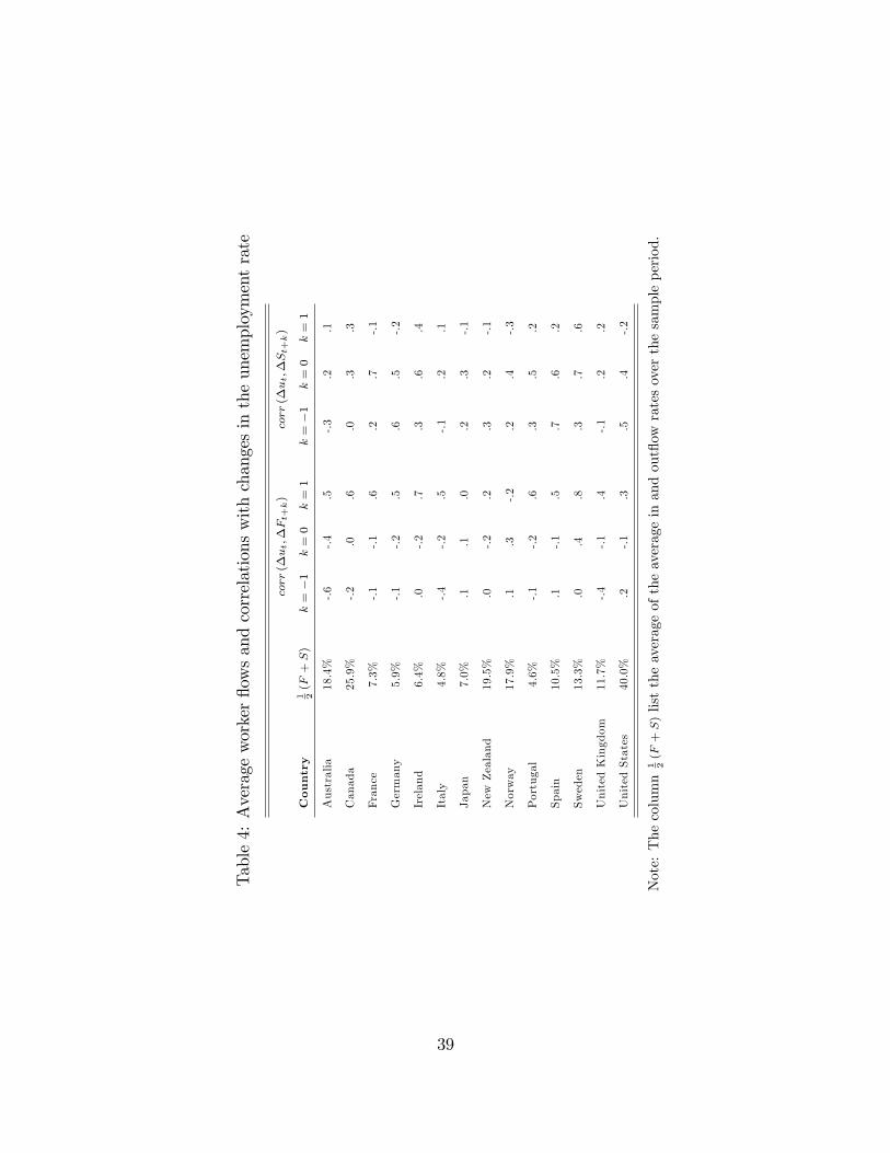
Table4:Averageworker�owsandcorrelationswithchangesintheunemploymentrate

corr(�ut;�Ft+k)

corr(�ut;�St+k)

Country

1 2(F+S)

k=�1

k=0

k=1

k=�1

k=0

k=1

Australia

18.4%

-.6

-.4

.5-.3

.2.1

Canada

25.9%

-.2

.0.6

.0.3

.3

France

7.3%

-.1

-.1

.6.2

.7-.1

Germany

5.9%

-.1

-.2

.5.6

.5-.2

Ireland

6.4%

.0-.2

.7.3

.6.4

Italy

4.8%

-.4

-.2

.5-.1

.2.1

Japan

7.0%

.1.1

.0.2

.3-.1

New

Zealand

19.5%

.0-.2

.2.3

.2-.1

Norway

17.9%

.1.3

-.2

.2.4

-.3

Portugal

4.6%

-.1

-.2

.6.3

.5.2

Spain

10.5%

.1-.1

.5.7

.6.2

Sweden

13.3%

.0.4

.8.3

.7.6

UnitedKingdom

11.7%

-.4

-.1

.4-.1

.2.2

UnitedStates

40.0%

.2-.1

.3.5

.4-.2

Note:Thecolumn

1 2(F+S)listtheaverageoftheaverageinandout�ow

ratesoverthesampleperiod.

39

Figure 1: Average in- and out�ow rates across countries.

40

Figure 2: In- and out�ow rates (log-scale in percentages) for Anglo-Saxon and Nordic coun-tries, and Japan

41

Figure 3: In- and outlfow rates (log-scale in percentages) for Continental European countries.

42

Figure 4: Actual versus steady state unemployment in four illustrative countries.

43

Figure 5: Steady-state versus non-steady-state decomposition of unemployment �uctuationsfor France.

44

Figure 6: Unemployment rate and worker �ows, Anglo-Saxon and Nordic countries, andJapan.

45

Figure 7: Unemployment rate and workers �ows, Continental European countries.

46