1

Understanding Labour Market Frictions: An Asset Pricing Approach

By

Parantap Basu1 Department of Economics and Finance

University of Durham UK

Revised, July 2008 Bulletin of Economics Research, Forthcoming

Abstract

Labour market friction is viewed in terms of the market value of an employed worker as opposed to the position of the Beveridge curve. This market value of an installed worker, which I call Tobin’s Q of a worker, is inversely proportional to the average quality of the match between employers and workers. Based on this measure, I find that the labour market friction rises during a period of productivity boom. This phenomenon is indirectly supported by the data where it is found that the relative value of a worker with respect to tangible capital shows a positive association with the TFP. The model suggests that firms may be compromising the quality of a skill match during a period of tight labour market condition.

1 Without implicating I would like to thank John Cochrane for inspiring me to undertake this project. Thanks are due to Martin Robson and Weshah Razzak for constructive comments. Anurag Banerjee is acknowledged for help on a technical issue. The paper significantly benefited from insightful comments from an anonymous referee. Thanks are also due to Mauricio Armellini and Soyeon Lee for able research assistance.

2

1. Introduction

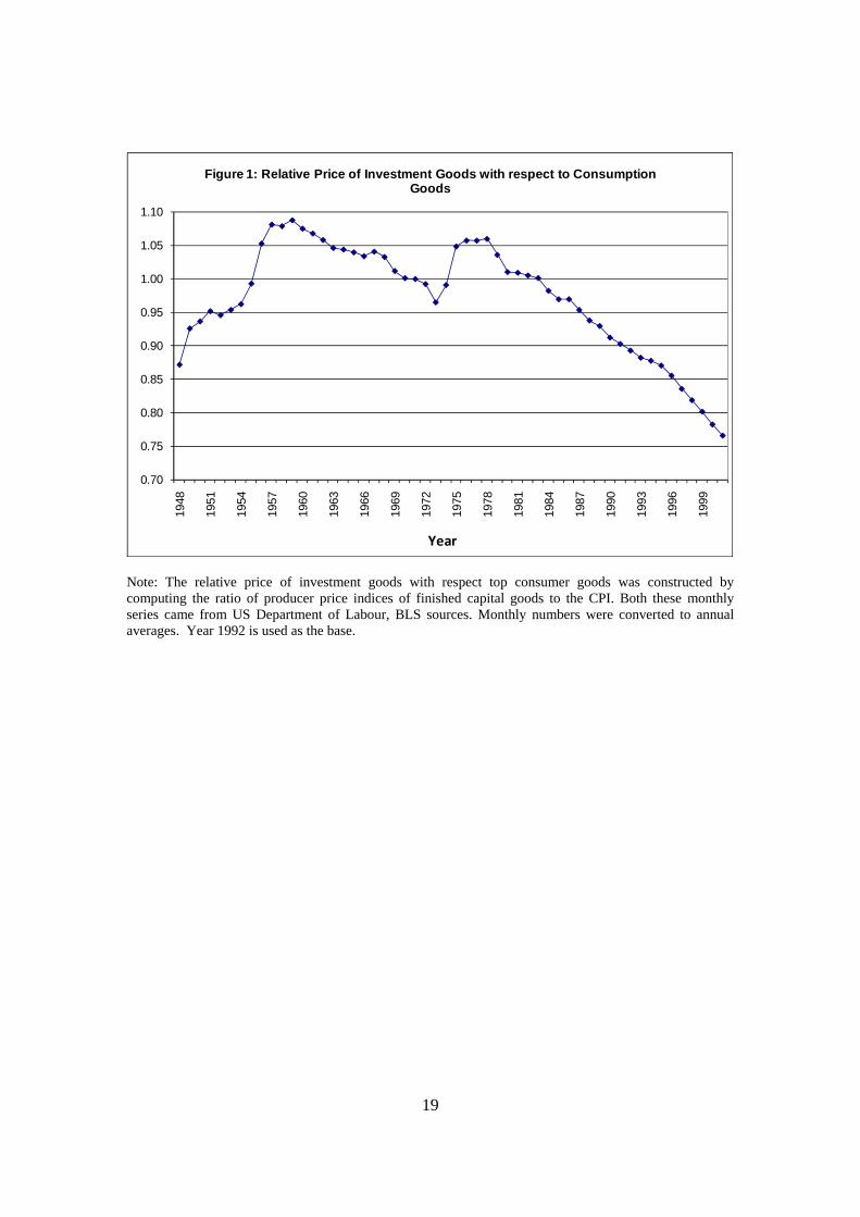
The relative price of investment to consumer goods has significantly declined over time in

the US. This decline is particularly noticeable in the 80s, which coincided with the great

period of moderation of output volatility. Figure 1 plots the ratio of US producer price

index of finished capital goods to the consumer price index. Following the oil shock in

the early 70s, there is a steady decline in this relative price of investment goods, which

reconfirms the decrease in capital market frictions in the 80s. A number of papers ascribe

this recent decline to elimination of investment frictions (Greenwich, Hercowitz and

Krusell, 2000; Chari, Kehoe and McGrattan, 2007). Although there is a near consensus

that the degree of capital market frictions in the US has substantially decreased recently,

less is known about labour market frictions.

Following the work of Pissarides (1985), by labour market friction I mean the

degree of mismatch between the worker and the employer. Little is known about this job-

matching variable at the aggregate level. A sizable literature focuses on the behaviour of

the unemployment-vacancy relationship (known as the Beveridge curve) as a measure of

this friction. There are both empirical and theoretical limitations of this Beveridge curve

based approach. Vacancies are usually measured by the help-wanted index which is less

reliable particularly after the internet revolution when job openings are mostly available

online. Valletta (2005) attempts to correct this deficiency by creating a synthetic job

vacancy ratio and argues that the Beveridge curve has shifted inward in the 80s after an

outward shift in the 70s. Shimer (2005) argues that the vacancy-unemployment ratio has

a remarkable volatility which makes it difficult to arrive at a definitive conclusion about

the time path of the labour market frictions. 2

Due to this limitation of the Beveridge curve based analysis I suggest a new

measure of labour market frictions based on asset pricing principles. From the firm’s

perspective, a higher probability of a worker-firm match can be thought of as higher

productivity of the firm’s search effort. If firms can efficiently search such that the

likelihood of a worker-firm match is higher, it will lower the market value of the already

employed workers. The reason is simply that the incumbent workers are easily

2 Hornstein et al. (2005) extend Shimer’s (2005) work and find additional problems in replicating the observed unemployment-vacancy fluctuations using the extant matching models.

3

replaceable because of the higher productivity of the firm’s search effort. Therefore,

these currently employed workers receive less rent to their skills in an environment where

the skill-match probability is higher. Thus one expects that the skill premium of an

incumbent worker will be lower when there is less labour market friction.

The market value of an incumbent worker can be thought of as the Q value, which

is reminiscent of Tobin’s (1969) Q measure. While Tobin’s Q measure is mostly applied

to physical or tangible capital, I propose to apply this measure to human capital and use it

to derive a new measure of labour market friction. A higher Q of an incumbent worker

thus signals a higher friction in the labour market. This asset-based measure of labour

market friction is motivated by Chari, Kehoe and McGrattan (2007) (C-K-M hereafter)

who suggest a measure of investment friction based on relative price of investment

goods. The scope of my paper differs in two important ways from C-K-M (2007). First,

while the principal focus of C-K-M is business cycle accounting in terms of various

frictions, my scope is limited to the understanding of labour market friction alone. Such a

friction is interpreted as a wedge on the human capital investment of the firm which is

driven by a fundamental TFP shock. Second, C-K-M does not view labour employment

in terms of an investment decision of the firm. 3

I employ a production based asset-pricing model based on the work of Merz and

Yashiv (2007) and Cochrane (1991) to derive the Tobin’s Q of an incumbent worker. By

construction, this Tobin’s Q is inversely related to the firm’s recruitment productivity.

The Q of the worker shows endogenous fluctuations driven by the TFP shock. Parallel to

investment friction, in my model, more friction in the labour market means a higher

Tobin’s Q of the existing worker. Using a calibrated version of this model, I estimate the

economy-wide matching probability based on the US aggregate data and find that it is

strongly countercyclical. This basically means that the quality of the worker-employer

match deteriorates during a boom. The implication is that firms compromise on the match

quality in hiring new employees in an economy with a tight labour market. 3 C-K-M (2007) provide a framework to account for business cycles in terms four frictions, namely efficiency wedge, labour wedge, investment wedge and the government consumption wedge. Their methodology of business cycle accounting has been recently criticised by Christiano and Davis (2006) referred C-D hereafter. While both C-K-M and C-D papers are very insightful in business cycle accounting and are fairly general in their scope, neither C-K-M nor C-D have human capital investment in their models and neither of them address the issue of labour market friction in a production based asset pricing framework as I do.

4

The plan of the paper is as follows. In the following section, I report some

stylized facts about the time series behaviour of the relative price of labour in terms of

capital. In section 3, a production-based asset-pricing model is laid out to show the precise

relationship between the labour market friction and the value of a worker. Section 4

reports some calibration results. Section 5 concludes.

2. Capital and Labour Market Frictions: Some Stylized Facts

Motivated by the relative price-based measure of input frictions as in Greenwood et al.

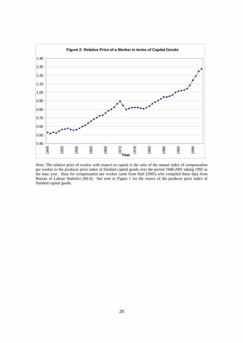
(2000), I calculate the relative price of a worker with respect to capital for the US

economy over the period 1948-2001 to arrive at a measure of labour market friction

relative to capital market friction. This relative price is measured by the ratio of the

annual index of compensation per worker to the producer price index of finished capital

goods over the period 1948-2001 taking 1992 as the base year. Data for compensation per

worker came from Hall (2005) who compiled these data from the Bureau of Labour

Statistics (BLS). The producer price index of finished capital goods came from the US

Department of Labour, BLS. Figure 2 plots the series. The relative price of a worker

shows a steady increase except for the period of the oil shocks during 1973-74 when all

producer prices increased.

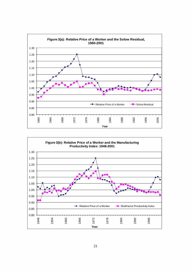
In the next step, I examine the cyclical behaviour of the relative price of a worker.

I use the total factor productivity (TFP) as an indicator of the business cycle. In order to

verify the robustness of the key results, two series for TFP are used. The first series is the

Solow residual based on non-farm output, aggregate hours worked and non-residential

fixed assets covering the period 1960-2001 for which an overlapping series for all three

are available. 4 The second slightly longer series is the annual manufacturing multifactor

productivity index obtained from the Bureau of Labour Statistics. This series is used as a

proxy for TFP to check for the robustness of results. The correlation coefficient between

these two TFP series is 0.95. Figures 3(a) and 3(b) plot the total factor productivity

(TFP) index and the relative price of worker after taking out a linear trend component

from each series. Both plots show very similar pattern. The cyclical component of the 4 The Solow residual is constructed by running a regression of the log of real GDP in the non-farm business sector, (series PRS85006043 from BLS), aggregate hours worked, as above, and the real non-residential fixed assets obtained from BEA Survey of Current Business.

5

value of worker positively correlates with the cyclical component of the TFP shock. The

correlation coefficient between these two series is 0.73 for Figure 3(a) and 0.66 for Figure

3(b). The relative price of worker rises during a period of TFP boom.5

In the rest of the paper, I argue that this relative price of worker with respect to

capital can be interpreted as the Tobin’s Q of an incumbent worker. I also argue that this

procyclical behaviour of a worker’s Tobin’s Q is driven by a decrease in the quality of the

match between workers and the employers during an expansion. This quality of the match

is measured by the productivity of the recruitment efforts. As the labour market tightens

during a boom, firms start compromising on the quality of the match while recruiting.

This makes already employed workers more valuable to the firm. Based on this analysis,

I argue that the Tobin’s Q of a worker is a reasonable measure of labour market friction as

opposed to unemployment-vacancy ratio. To make this point transparent, in the next

section, I focus on the production sector of the economy and develop a labour based asset-

pricing model.

3. The Model

The production-based asset-pricing model is an adaptation of Merz and Yashiv (2007).6

The production sector consists of identical firms sharing the same production and

investment technology facing a market wage rate, wt. The timeline is as follows. At the

start of date t, the firm observes a TFP shock tε and produces output with the

predetermined tangible capital Kt and the human resources Nt using the following Cobb-

Douglas production function:

ααε −= 1tttt NKY (1)

where α is the capital share in output. The firm then disburses the existing employees a

real wage of wt. Finally it undertakes two types of investment decisions: investment in

5 The procyclcial movement of the value of worker is robust to the choice of detrending method. I also looked at the correlation between Hodrick-Prescott detrended series for real GDP and the value of worker. The correlation coefficient between these two series is 0.50. 6 Merz and Yashiv (2006) use a production based asset-pricing model of the type pioneered by Cochrane (1991). Their innovation is to show that the market value of a firm can be decomposed into the value of capital and the value of labour.

6

tangible capital It and posting of new vacancy, Vt. The cost of posting new vacancies, Xt

is proportional to the number of posting as follows:7

tt aVX = ; with 0>a (2)

Investment in tangible capital augments firm’s physical capital following a standard

linear depreciation rule:

ttt IKK +−=+ )1(1 δ (3)

where δ is the constant rate of depreciation of physical capital.

Regarding the latter investment, I follow Merz and Yashiv (2007), to postulate the

following law of motion for the employees:

tttt VqNN +−=+ )1(1 ψ (4)

where )1,0(∈ψ is an exogenous job destruction rate, and qt is the probability that a

posted vacancy will be filled or equivalently it is the match probability between a worker

and an employer. Alternatively qt can also be interpreted as the quality of the match

because it is positively related to the productivity of a firm’s spending on recruitment.8 It

will be shown later that qt is endogenous in this model and determined by the firm’s

valuation of a worker, which in turn depends on economic fundamentals. Throughout my

analysis I ignore any convex adjustment costs of changing capital and labour. Hall (2004)

finds that adjustment costs are relatively minor and do not explain large part of the

variation of the corporation value.

The representative firm facing a constant discount factor ρ solves the following

problem9:

Max }]{[ 1

00 ttttttt

t

t IXNwNKE −−−−∞

=∑ ααερ (P)

s.t. (2) through (4) , given K0 , N0.

7 An introduction of a quadratic posting cost will give rise to nonlinearity which is akin to employment adjustment cost. In principle, one does not expect the main results about Tobin’s Q of a worker to change much except that the firm needs to worry about a secondary cost of adjusting employment while making recruitment. 8 Note that the marginal return to recruitment spending is: .//1 aqXN ttt =∂∂ + 9 I ignore any convex adjustment cost in this benchmark model. There is, however, some built in adjustment cost of shifting resources from tangible to intangible capital. The firm incurs a relative price of 1/qt to switch from tangible to intangible investment.

7

The TFP shock tε is specified as a geometric random walk as follows:10

11 lnln ++ += ttt ξεε (5)

where 1+tξ ~N(0, 2σ )

The first order conditions with respect to I and X are as follows:

I: [ ]δαερ α −+= −++ 11 1

11 ttt kE (6)

X: ])1()1([ 11111

1 −++++

− −+−−= tttttt aqwkEaq ψαερ α (7)

where kt is the capital/employment ratio at date t. Given the random walk nature of the

TFP shock, it is straightforward to verify that the capital-employment ratio is:

α

δρεαρμ −

+ ⎥⎦

⎤⎢⎣

⎡−−

=1

1

11 )1(1

ttk (8)

where

⎟⎟⎠

⎞⎜⎜⎝

⎛=

2exp

21

σμ (9)

The first order conditions (6) and (7) can be rewritten in the following valuation equation form: I: [ ]211 +++ += t

kttt KCFEK ρ (10)

X: ⎥⎦

⎤⎢⎣

⎡+=

+

++

+

1

21

1

t

tnt

t

tq

aNCFq

aN ρ (11)

where tttt

kt IKkCF −= −1ααε and tttttt

nt XNwNkCF −−−= ααε )1( .

10 According to Prescott (1986) US TFP is a near random walk process while I assume that it is an exact random walk. Banerjee (2001) show that the first order forecast sensitivity due to difference stationary specification when the process is truly trend stationary is zero. See also Banerjee and Basu (2001) for a related paper. Moreover, I also performed a unit root test for the logarithm of the TFP series used in the following section. One cannot reject the null of a unit root.

8

Using (10) and (11) one can have the following value decomposition for the firm’s market

value ( MtMV )

NtMVK

tMVMtMV += (12)

where

1+= tKKtMV (13)

tqtaNN

tMV 1+= (14)

The Tobin’s Q of capital ( 1/ +tKKtMV ) is unity while the Tobin’s Q of a worker

( 1/ +tNNtMV ) is inversely proportional to the match probability qt. The match probability

qt drives a wedge between the Tobin’s Q of capital and the Tobin’s Q of labour.

Using (7) and (8), one can write the following Tobin’s Q equation for a worker:

])1()1(1

)1( 111

111

11

11 −

++−−−− −+−⎥

⎦

⎤⎢⎣

⎡−−

−= tttttt qEawEaq ψρρδρ

αρεμαρ αα

αα (15)

This valuation equation is just like a standard asset pricing equation. The worker is valued

as an asset to the firm. The Tobin’s Q of an installed (employed) worker is typically the

expected present value of cash flows or surplus arising from his/her continued

employment. This cash flow is the difference between worker’s expected productivity

and the expected real wage.

Wage Determination

The wage determination story is the same as in Merz and Yashiv (2007). Real wage is

determined by a Nash bargaining between worker and the firm assuming that both have

equal bargaining power. Hiring an additional worker generates a surplus of for the firm

{ ttt wqaMPN −−+ )/)(1( ψ } and ( )tt bw − for the worker where bt is the unemployment

9

benefit which is the value of the outside option of the worker. In other words the real

wage ( tw ) is given by:

φφψ −−−−+= 1][])/)(1(max[arg tttttt bwwqaMPNw (16)

where tMPN is the marginal product of labour at date t and φ is the bargaining strength

of the firm vis-à-vis worker. Assuming that the unemployment benefit is an exogenously

specified constant fraction of tw , wage equation in (16) is given by:

)]/)(1()1)[(1( tttt qakw ψεαφ α −+−−= (17)

Vacancies and Tobin’s Q of a Worker Without any loss of generality, assume that a fixed fraction of the labour force

participates in the labour market. In the absence of population growth this means that

labour is inelastically supplied which I normalize at the unit level.11 Using (4) one gets

the following vacancy equation

tt q

V ψ= (18)

Next substituting the wage equation (17) into (15) and using the method of undetermined

coefficient, one arrives at the following solution for the worker’s Tobin’s Q:12

)1/(11 αε −− Ω= ttaq (19)

11 The assumption of an inelastic labour supply can be easily micro founded. Think of liquidity constrained

workers who receive utility from consumption ( tc ) and leisure tlT−−

where tl is the choice of work hours

and −T is a fixed time endowment. Each worker thus solves a static utility maximization problem: Max

)ln(ln tt lTc −+−

s.t. ttt lwc = . The optimal labour supply and leisure are 2/−T . Given a fixed number

of workers, the immediate implication is that the labour supply is a constant. 12 For the existence of the Tobin’s Q equation one requires a convergence condition that )1/(1

1αμ − <1

which is met for a sufficiently small value of 2σ . The conventional estimate of the variance of Solow residual is small. Prescott (1986) fixes it at .00763 which I use in the calibration section 4.

10

where )1/(

)1/(11

)1/(11

)1(1)1(5.1

)1(5. αα

α

α

δραρ

μψρ

μαρ −

−

−

⎥⎦

⎤⎢⎣

⎡−−⎥

⎥

⎦

⎤

⎢⎢

⎣

⎡

−−

−=Ω (20)

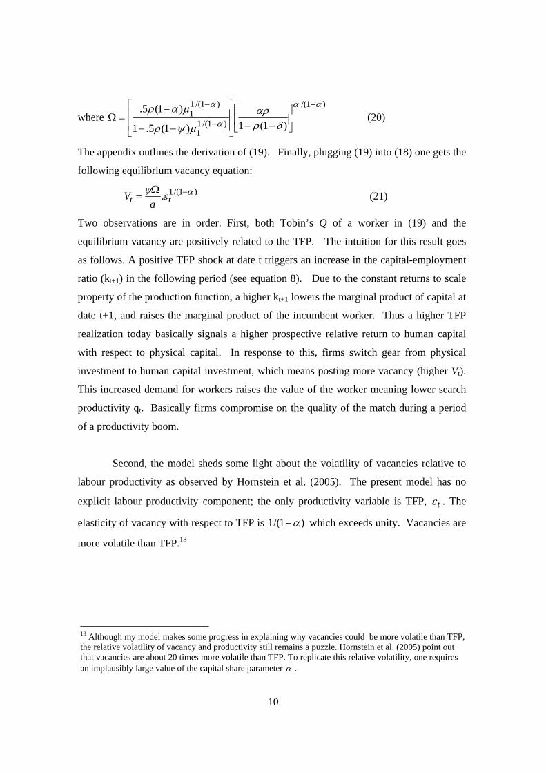
The appendix outlines the derivation of (19). Finally, plugging (19) into (18) one gets the

following equilibrium vacancy equation:

)1/(1. αεψ −Ω= tt a

V (21)

Two observations are in order. First, both Tobin’s Q of a worker in (19) and the

equilibrium vacancy are positively related to the TFP. The intuition for this result goes

as follows. A positive TFP shock at date t triggers an increase in the capital-employment

ratio (kt+1) in the following period (see equation 8). Due to the constant returns to scale

property of the production function, a higher kt+1 lowers the marginal product of capital at

date t+1, and raises the marginal product of the incumbent worker. Thus a higher TFP

realization today basically signals a higher prospective relative return to human capital

with respect to physical capital. In response to this, firms switch gear from physical

investment to human capital investment, which means posting more vacancy (higher Vt).

This increased demand for workers raises the value of the worker meaning lower search

productivity qt. Basically firms compromise on the quality of the match during a period

of a productivity boom.

Second, the model sheds some light about the volatility of vacancies relative to

labour productivity as observed by Hornstein et al. (2005). The present model has no

explicit labour productivity component; the only productivity variable is TFP, tε . The

elasticity of vacancy with respect to TFP is )1/(1 α− which exceeds unity. Vacancies are

more volatile than TFP.13

13 Although my model makes some progress in explaining why vacancies could be more volatile than TFP, the relative volatility of vacancy and productivity still remains a puzzle. Hornstein et al. (2005) point out that vacancies are about 20 times more volatile than TFP. To replicate this relative volatility, one requires an implausibly large value of the capital share parameter α .

11

4. Calibration

Parameter Values

There are six parameters of interest: α , δ , ,ρ ψ , 2σ , a and φ . Following Prescott

(1986), I set the benchmark values, α = .36, and δ =0.1 (annual data), 96.=ρ and 2σ is

fixed at .00763. There is no published estimate of the parameter ψ . The closest one is the

average job separation rate of 3% in the US economy over the period 1948-2001 found in

Hall (2001). The remaining job posting cost parameter a in equation (2) is scaled to

ensure that the maximum value of job match probability qt equals unity. Without any loss

of generality, the value of φ is fixed at 0.5. 14

Model and Actual Tobin’s Q of a Worker

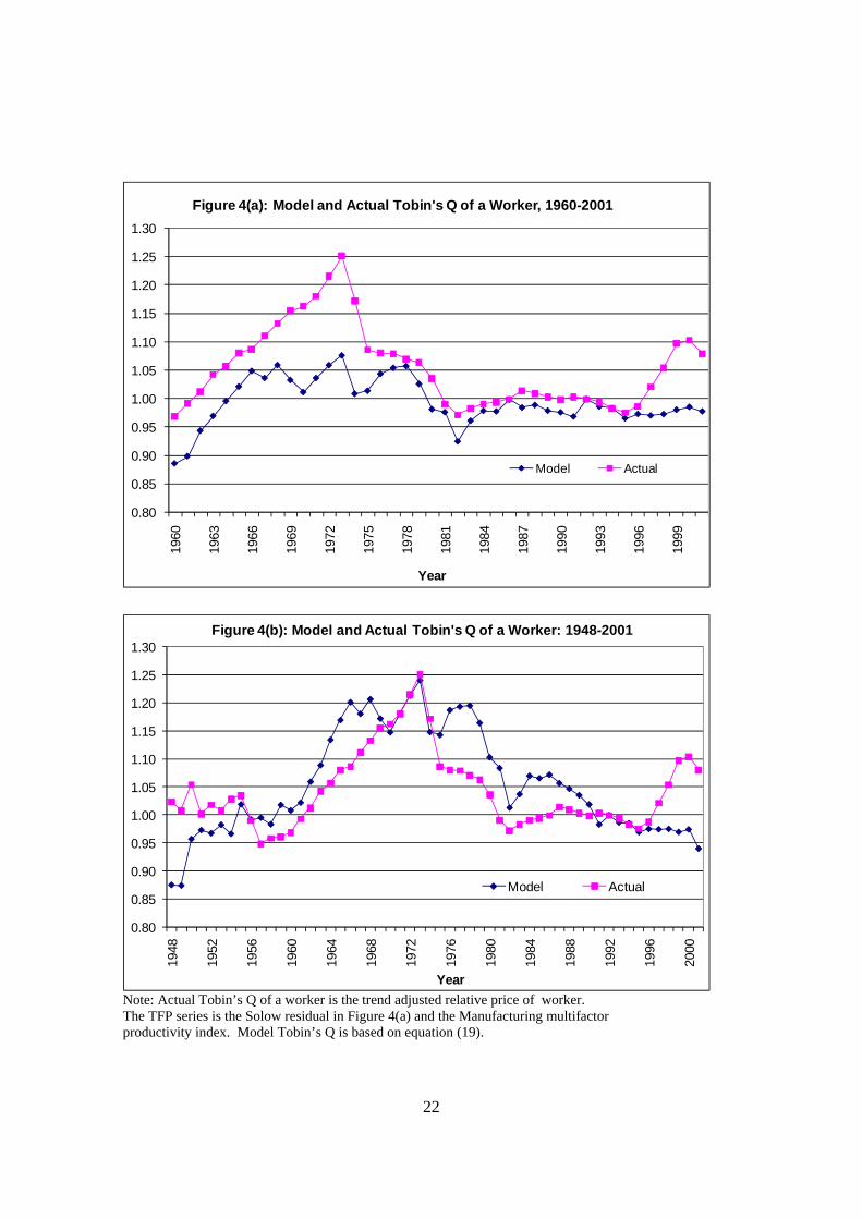
Using the baseline parameter values and the observed series for the TFP, I next compute

the model Tobin’s Q of a worker. Since the model has no implication for growth, I

detrend the TFP by passing a linear trend through it and then computing the residual. This

TFP residual is then plugged into the Tobin’s Q equation (19) given the baseline

parameter values. This series is then compared with the detrended actual relative price of

a worker. Figures 4(a) and 4(b) plot the results for both TFP series. To make these series

comparable, all are scaled such that they are unity for the base year 1992. The model

performs reasonably well in tracking down the business cycle fluctuations in the relative

price of a worker. The correlation is 0.73 for Figure 4(a) and 0.67 in Figure 4(b).15 The

relationship between actual and model’s Q in Figures 4(a) and 4(b) are remarkably similar

to the relationship between TFP and the actual Tobin’s Q in Figures 3(a) and 3(b). This

is expected because the TFP drives the model’s Tobin’s Q as shown in equation (19).

14 Changing the bargaining parameter has insignificant quantitative effect on the Tobin’s Q of a worker. 15 I also performed sensitivity analysis around the baseline parameter values which I do not report here for brevity. The correlation between the model and actual Tobin’s Q of a worker is reasonably robust to changes in the parameters.

12

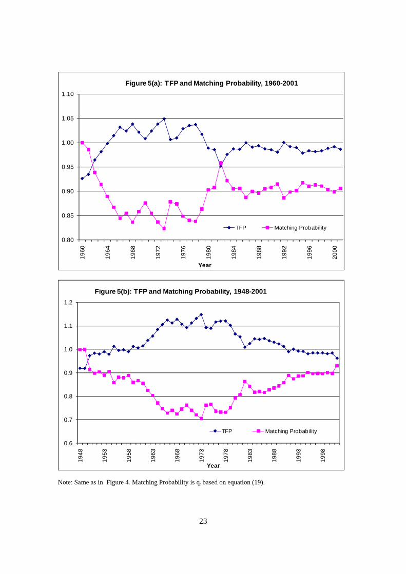
An Estimate of the Employer-Worker Match Probability

In this section, I estimate the match probability qt based on the reduced form equation

(19). Figures 5(a) and 5(b) plot this matching probability and the detrended TFP

series.16 The matching probability declined during the 70s and then it revived in the 80s

while TFP shows the opposing pattern. The matching probability increased during the

80s when there was a productivity slowdown. The result is robust with respect to the

choice of the TFP series. These results reinforce my hypothesis that the quality of the

match shows a countercyclical pattern.

Does Skill Match Worsen During a Boom?

The model predicts that the skill match and the consequent labour market friction worsen

during a boom. There are three ways one can validate this prediction. First, the model

predicts a procyclical movement of the Tobin’s Q of a worker which holds up with the

data as seen in Figure 4. The inverse of this Tobin’s Q of a worker is proportional to the

skill match probability. Second, my results are consistent with Valletta (2005) who finds

that the US Beveridge curve shifted out during the 70s and then shifted back in during the

80s. The shift of the Beveridge curve appears countercyclical to productivity which is

consistent with the model’s prediction. 17 Third, there is also some international evidence

of the procyclicity of the labour market friction. Hall and Scobie (2005) and Razzak

(2007) document that the growth rates of output and labour productivity are relatively

higher in Australia compared to New Zealand particularly after 1995. This productivity

gain coincided with a period of higher capital intensity and a higher relative price of

labour in Australia. Razzak (2007) confirms that during the same period Australia

experienced an increase in the number of vacancies as well. These international stylized

facts accord well with my model’s prediction that the labour market friction increases

during a productivity boom.

16 The TFP series is also normalized at unity taking 1992 as the base year. 17 A lesser productive match during a tighter labour market means that the firm strikes a quantity-quality trade off which could have an adverse effect on TFP. While this is a possibility, I do not model TFP in here. In my model, the TFP is the fundamental shock which means that the causality runs from TFP to the labour market friction not the other way round. In a future paper, one can investigate how this quantity-quality trade off could impact TFP.

13

Investment Wedge vs. Capital Wedge

In the present setting, the labour market friction is viewed as the market value of an

incumbent worker. The skill match probability tq drives a wedge between the Tobin’s Q

of human capital and the Tobin’s Q of physical capital. In other words, the labour market

friction is nothing but a wedge on the firm’s investment in human capital vis-à-vis

physical capital. This wedge-view of labour market friction draws on the business cycle

accounting (BCA) methodology as in Chari, Kehoe and McGrattan (2007). Christiano

and Davis (2006) point out a major flaw of this BCA principle. Since investment has an

intertemporal dimension, any wedge on it depends on future expectations of the rational

agents. How one models this wedge may thus matter for the robustness of the results.

Chakraborty (2008), and Kobayashi and Inaba (2006) also point out that the BCA results

for Japan are sensitive to how one models investment wedge. If it is modeled as a wedge

on gross returns to capital instead, the results might change.

In the present paper, I choose to model labour market friction as an investment

wedge instead of a capital wedge primarily because of two reasons. The first reason is

methodological. The investment wedge directly identifies the matching probability tq via

the Tobin’s Q equation of the worker while the capital wedge does not. 18 This approach

to understand labour market friction using asset pricing principle is novel in the literature

and demonstrates a convenient marriage between labour economics and finance. The

second reason is that my formulation is data friendly. The matching probability can be

directly estimated from the available macro data.

The issue still remains whether the key prediction of the model that labour

market friction is pro-cyclical holds up with an alternative capital-wedge view of the

friction. I explore this issue in the Appendix B by working out a perfect foresight version

of the present model by replacing the investment wedge tq by human capital wedge Ntτ .

18 To see this point clearly, note that the marginal return to human capital investment (recruitment) is

aqXN ttt //1 =∂∂ + based on (2) and (4). The marginal return to physical capital investment

tt IK ∂∂ + /1 based on (3) is 1. The marginal rate of transformation between physical capital and human capital (which is the ratio of these two respective marginal returns) uniquely identifies the skill match probability tq which is our key indicator of labour market friction. Such an identification of the skill matching probability may not be possible if the labour market friction is viewed as a human capital wedge.

14

The pro-cyclical behaviour of the friction with respect to the TFP is reasonably robust for

plausible parametric restriction. 19

5. Conclusion

There is no consensus whether the labour market friction has increased or decreased in the

US economy over the last few decades. The conventional Beveridge curve based

explanation of labour market friction is problematic because of the remarkable volatility

of the vacancy/unemployment ratio. In this paper, I take an asset pricing approach to

understand the labour market friction. The labour market friction is viewed as an implicit

tax on a firm’s investment in human capital. The model suggests that this wedge is

inversely related to the firm’s recruitment productivity which in turn depends on the

fundamental TFP shock driving the economy. In a booming economy, the recruitment

productivity of the firm is lower due to tight labour market conditions. As a result, the

incumbent workers enjoy a rent in terms of a higher Tobin’s Q. Viewed from this

perspective, I conclude that the labour market friction gets aggravated during a period of

TFP boom suggesting that the firm compromises the quality of the match in a tighter

labour market condition. This pro-cyclical behaviour of the labour market friction is

reasonably robust with respect to alternative formulation of labour market friction such as

a human capital wedge. The model receives some empirical support from the labour

market experiences of the US and Australia.

The public policy implication is that the government may need to invest more

resources in job training program during a period of productivity boom when acute skill

shortages could arise. A wide range of vocational courses can be set up at adult skill-

centers to avoid these skill shortages. This would lower the Tobin’s Q of an employed

worker and eliminate the rent that an incumbent worker receives during a productivity

boom. A useful extension of this paper would be to model such an optimal education

policy.

19 A comprehensive analysis of this robustness issue also involves an analysis with alternative stochastic specification of TFP as well as model specification, which is beyond the scope of this paper. The present model does not include a household sector. In a future paper, I plan to examine this issue using a dynamic stochastic general equilibrium model with various adjustment costs.

15

Appendix A

Derivation of Equation 19

Plug (17) into (15) to obtain

11

)1/(11 )1(5. −+

−− −+= tttt aqEAaq ψρε α (A.1)

where

[ ] )1/()1/(1

1 )1(1)1(5.

ααα

δραρμαρ

−−

⎥⎦

⎤⎢⎣

⎡−−

−=A

Conjecture a solution

)1/(11 αε −− Ω= ttaq (A.2)

where Ω is a coefficient to be determined by the method of undetermined coefficient.

Upon substitution in (A.1) and using the geometric lognormal random walk property of

the TFP process }{ tε one obtains:

)1/(1)1/(11

)1/(1)1/(1 )1(5. αααα εμψρεε −−−− Ω−+=Ω ttt A (A.3)

One can now uniquely solve Ω which gives (20) and confirms that the conjecture (A.2) is

right. This proves (19) and (20). //

Appendix B

Case when labour market friction is modeled as a human capital wedge

Let a positive fraction Ntτ represent the proportional wedge on the gross return on human

capital. In a similar vein as in Kobayashi and Inaba (2006), I assume perfect foresight in

the sense that the sequences of the human capital wedge, { Ntτ } and the TFP, { tε } are

known to the firm at date 0. The representative firm’s problem (P) now changes to:

Max ])1([ 1

0tttt

Ntttttt

t

t IXNMPNNwNK −−−+−−∑ −∞

=ψτερ αα

s.t. (2), (3) and (4).

16

Since the investment wedge is replaced by the capital wedge, set tq equal to unity. For

simplicity, set the posting cost a equal to unity. The TFP }{ tε is assumed to be

exogenously given. The human capital wedge, Ntτ is endogenous. The problem is to

uncover the relationship between TFP and the human capital wedge sequence { Ntτ }. In

other words, one is interested in signing the derivative t

Ntετ∂∂

.

The first order conditions are:

tI : ]1})1(1([1 1111 δαταερ α −+−−= −

+++ tNtt k (B.1)

tX : 1= )]1)(1()1)()1(1([ 11111Nttt

Ntt wk +++++ −−+−−−− τψαταερ α (B.2)

The wage bargaining equation (16) changes to:

φφψτ −−−−+−= 1][]))1()(1max[(arg ttttNtt bwwMPNw (B.3)

which yields the following wage equation:

]1)1)[(1)(1( ψεατφ α −+−−−= ttNtt kw (B.4)

which upon substitution in (B.2) gives:

)]1)(1()1)()1([(1 11111Nttt

Nt

Nt k +++++ −−+−+−= τψφεααττφρ α (B.5)

From (B.1) solve 1+tk as:

α

δρετααρ −++

+ ⎥⎥⎦

⎤

⎢⎢⎣

⎡

−−

−−=

11

111 )1(1

})1(1{ tNt

tk (B.6)

17

The model is thus summarized by two equations, (B.5) and (B.6) with two endogenous

variables 1+tk and Nt 1+τ , and one exogenous variable 1+tε . Based on (B.6), it follows

that 1+tε impacts 1+tk directly as well as indirectly via its effect on Nt 1+τ . Define the

right hand side of (B.6) as a function h(.). Thus (B.6) can be written in a compact form as

follows:

))(,( 1111 ++++ = tNttt hk ετε (B.7)

One can thus write the following derivative based on (B.7) using the implicit function

theorem:

1

1

111

1 .+

+

+++

+∂

∂

∂

∂+

∂∂

=t

Nt

Nttt

t hhddk

ετ

τεε (B.8)

From (B.6) verify that the right hand side terms in (B.8), 01>

∂∂

+t

hε

and Nt

h

1+∂

∂

τ <0.

To determine the sign of 1

1

+

+∂

∂

t

Nt

ετ

, differentiate (B.5) and employ (B.8) and obtain:

Δ

+−=

∂

∂ +++

+

+ααττφ

ετ 111

1

1 })1({ tNt

Nt

t

Nt k

(B.9)

where

}])1)(1.{()1([

)]1)(1()1)([(

111

111

11

Nt

NtN

ttt

tt

hk

k

+++

−++

++

+−−∂

∂−−

−−+−−=Δ

αττφτ

εαα

ψφεααφ

α

α

(B.10)

18

Note that the numerator of (B.9) is positive. The second term of the denominator Δ is

positive because Nt

h

1+∂

∂

τ <0 from (B.6). A sufficient condition for the first term of the

denominator to be positive is that φα < . Thus if φα < , 1

1

+

+∂∂

t

Ntετ >0.

A sufficient condition for the human capital wedge to be pro-cyclical with

respect to the TFP is, therefore, φα < . The intuition for this result is similar as in the

case of an investment wedge. A higher prospective TFP translates into a higher

capital:labour ratio which drives down the marginal product of tangible capital, MPK and

boosts the marginal product of intangible capital, MPN. If workers have weak bargaining

power vis-à-vis firms in the sense that their share of the surplus φ−1 is less than their

what they contribute to total output ( α−1 ), they pay a greater wedge. It is difficult to

get a reliable estimate of the rent sharing parameter φ . Mumford and Dowrick (1994)

point out the methodological problem in estimating this parameter. Their estimate based

on coal industry of New South Wales, Australia suggests that the estimate of worker’s

rent sharing is about 10% which has to be interpreted with caution. Given this caveat and

also given that the US capital share in GDP is about 0.36, the condition φα < appears

like a plausible restriction.

19

0.70

0.75

0.80

0.85

0.90

0.95

1.00

1.05

1.10

1948

1951

1954

1957

1960

1963

1966

1969

1972

1975

1978

1981

1984

1987

1990

1993

1996

1999

Figure 1: Relative Price of Investment Goods with respect to Consumption Goods

Year

Note: The relative price of investment goods with respect top consumer goods was constructed by computing the ratio of producer price indices of finished capital goods to the CPI. Both these monthly series came from US Department of Labour, BLS sources. Monthly numbers were converted to annual averages. Year 1992 is used as the base.

20

Figure 2: Relative Price of a Worker in terms of Capital Goods

0.40

0.50

0.60

0.70

0.80

0.90

1.00

1.10

1.20

1.30

1.40

1948

1953

1958

1963

1968

1973

1978

1983

1988

1993

1998

Year

Note: The relative price of worker with respect to capital is the ratio of the annual index of compensation per worker to the producer price index of finished capital goods over the period 1948-2001 taking 1992 as the base year. Data for compensation per worker came from Hall (2005) who compiled these data from Bureau of Labour Statistics (BLS). See note to Figure 1 for the source of the producer price index of finished capital goods.

21

0.80

0.85

0.90

0.95

1.00

1.05

1.10

1.15

1.20

1.25

1.30

1960

1964

1968

1972

1976

1980

1984

1988

1992

1996

2000

Year

Figure 3(a): Relative Price of a Worker and the Solow Residual, 1960-2001

Relative Price of a Worker Solow Residual

0.80

0.85

0.90

0.95

1.00

1.05

1.10

1.15

1.20

1.25

1.30

1948

1954

1960

1966

1972

1978

1984

1990

1996

Year

Figure 3(b): Relative Price of a Worker and the Manufacturing Productivity Index: 1948-2001

Relative Price of a Worker Multifactor Productivity Index

22

0.80

0.85

0.90

0.95

1.00

1.05

1.10

1.15

1.20

1.25

1.30

1960

1963

1966

1969

1972

1975

1978

1981

1984

1987

1990

1993

1996

1999

Year

Figure 4(a): Model and Actual Tobin's Q of a Worker, 1960-2001

Model Actual

0.80

0.85

0.90

0.95

1.00

1.05

1.10

1.15

1.20

1.25

1.30

1948

1952

1956

1960

1964

1968

1972

1976

1980

1984

1988

1992

1996

2000

Year

Figure 4(b): Model and Actual Tobin's Q of a Worker: 1948-2001

Model Actual

Note: Actual Tobin’s Q of a worker is the trend adjusted relative price of worker. The TFP series is the Solow residual in Figure 4(a) and the Manufacturing multifactor productivity index. Model Tobin’s Q is based on equation (19).

23

0.80

0.85

0.90

0.95

1.00

1.05

1.10

1960

1964

1968

1972

1976

1980

1984

1988

1992

1996

2000

Year

Figure 5(a): TFP and Matching Probability, 1960-2001

TFP Matching Probability

0.6

0.7

0.8

0.9

1.0

1.1

1.2

1948

1953

1958

1963

1968

1973

1978

1983

1988

1993

1998

Year

Figure 5(b): TFP and Matching Probability, 1948-2001

TFP Matching Probability

Note: Same as in Figure 4. Matching Probability is qt based on equation (19).

24

References

Banerjee, A.N (2001), “Sensitivity of Univariate AR(1) Time-series Forecasts near the Unit Root”, Journal of Forecasting, Vol 20 Issue 3, pp. 203-229. Banerjee, A.N. and P. Basu (2001), “A Re-examination of Excess Sensitivity Puzzle when Consumers Forecast the Income Process”, Journal of Forecasting, Vol 20 Issue 5, pp. 357-356. Chakraborty, S (2008), “The Boom and the Bust of the Japanese Economy: A Quantitative Look at the Period 1980-2000,” Japan and the World Economy, Forthcoming. Chari V, P.J. Kehoe and E. McGrattan (2007), “Business Cycle Accounting,” Econometrica, 75, 3, 781-836. Christiano, L.J and J.M. Davis (2006), “ Two Flaws in Business Cycle Accounting,” Working Paper, Northwestern University. Cochrane, J.H. (1991), “Production Based Asset Pricing and the Link between Stock Returns and Economic Fluctuations,” Journal of Finance, 147:207-234. Hall. Greenwood, J, Z. Hercowitz and Krusell, P. (2000), "The role of investment specific technological change in the business cycle, European Economic Review, 44, 91-115. Hall, R.E. (2005), “Job Loss, Job Finding and Unemployment in the past Fifty Years,” NBER Macroeconomics Annual, pp. 101-137. Hall, R.E. (2004), “Measuring Factor Adjustment Costs,” Quarterly Journal of Economics, August, 119(3): 899-927. Hall J and G. Scobie (2005), “Capital Shallowness: A Problem for New Zealand?” New Zealand Treasury Working Paper, 05/05. Hornstein, A, P. Krusell and G. L. Violante (2005), “Unemployment and Vacancy Fluctuations in the Matching Model: Inspecting the Mechanism,” Economic Quarterly, Federal Reserve Bank of Richmond, 91, 3:pp.19-51. Kobayashi, K and M. Inaba (2006), “Business Cycle Accounting for the Japanese Economy,” Japan and the World Economy, 18: 418-440. Razzak W.A. (2007) “On the Dynamics of Search, Matching and Productivity in New Zealand and Australia,” International Journal of Applied Economics, Forthcoming.

25

Merz, M (1995), “Search in the Labour Market and the Real Business Cycle,” Journal of Monetary Economics, 36: 269-300. Merz, M and E. Yashiv (2007), “Labor and the Market Value of the Firm", American Economic Review 97:1419-1431, 2007. Mumford, K and S. Dowrick 91994), “Wage Bargaining with Endogenous Profits, Overtime Working and Heterogeneous Labor,” Review of Economics Statistics, 76,2, 329-336. Nickell, S, l. Nunziata, W. Ochel and G. Quintini (2003), “The Beveridge Curve, Unemployment and Wages in the OECD from 1960s to the 1990s, in Aghion, et al. Knowledge and Expectations in Modern Macroeconomics, Princeton University press. Pissarides, C.A. (1985), “Short run Dynamics of Unemployment, Vacancies and Real Wages,” American Economic Review, 75:676-690. Prescott. E.C. (1986), “Theory Ahead of Business Cycle Measurement,” Quarterly Review 10(4): 1-15. Shimer, R (2005), “The Cyclical Behavior of Equilibrium Unemployment and Vacancies,” American Economic Review, 95(1): 25-49. Tobin, J (1969), “A General Equilibrium Approach to Monetary Theory,” Journal of Money, Credit and Banking, 1(February): 15-29. Valletta, R.G. (2005), “Why has the US Beveridge Curve Shifted Back? New Evidence Using Regional Data,” Federal Reserve Bank of San Francisco, Reproduced.