Understanding Environmental Change and Biodiversity … · Understanding Environmental Change and...
160
Understanding Environmental Change and Biodiversity in a Dryland Ecosystem through Quantification of Climate Variability and Land Modification: The Case of the Dhofar Cloud Forest, Oman by Christopher S. Galletti A Dissertation Presented in Partial Fulfillment of the Requirements for the Degree Doctor of Philosophy Approved August 2015 by the Graduate Supervisory Committee: B.L. Turner II, Chair Patricia L. Fall Soe W. Myint ARIZONA STATE UNIVERSITY December 2015
Transcript of Understanding Environmental Change and Biodiversity … · Understanding Environmental Change and...
Understanding Environmental Change and Biodiversity in a Dryland Ecosystem through
Quantification of Climate Variability and Land Modification: The Case of the Dhofar
Cloud Forest, Oman
by
Christopher S. Galletti
A Dissertation Presented in Partial Fulfillment
of the Requirements for the Degree
Doctor of Philosophy
Approved August 2015 by the
Graduate Supervisory Committee:
B.L. Turner II, Chair
Patricia L. Fall
Soe W. Myint
ARIZONA STATE UNIVERSITY
December 2015

©2015 Christopher S. Galletti
All Rights Reserved
i
ABSTRACT
The Dhofar Cloud Forest is one of the most diverse ecosystems on the Arabian
Peninsula. As part of the South Arabian Cloud Forest that extends from southern Oman
to Yemen, the cloud forest is an important center of endemism and provides valuable
ecosystem services to those living in the region. There have been various claims made
about the health of the cloud forest and its surrounding region, the most prominent of
which are: 1) variability of the Indian Summer Monsoon threatens long-term vegetation
health, and 2) human encroachment is causing deforestation and land degradation. This
dissertation uses three independent studies to test these claims and bring new insight
about the biodiversity of the cloud forest.
Evidence is presented that shows that the vegetation dynamics of the cloud forest
are resilient to most of the variability in the monsoon. Much of the biodiversity in the
cloud forest is dominated by a few species with high abundance and a moderate number
of species at low abundance. The characteristic tree species include Anogeissus dhofarica
and Commiphora spp. These species tend to dominate the forested regions of the study
area. Grasslands are dominated by species associated with overgrazing (Calotropis
procera and Solanum incanum). Analysis from a land cover study conducted between
1988 and 2013 shows that deforestation has occurred to approximately 8% of the study
area and decreased vegetation fractions are found throughout the region. Areas around
the city of Salalah, located close to the cloud forest, show widespread degradation in the
21st century based on an NDVI time series analysis. It is concluded that humans are the
primary driver of environmental change. Much of this change is tied to national policies
and development priorities implemented after the Dhofar War in the 1970’s.

ii
DEDICATION
To Sanda and Lucy:
I love you

iii
ACKNOWLEDGMENTS
I would like to first thank my advisor and committee chair, Professor B.L. Turner
II, for all his hard work and support during the writing of this dissertation. Billie is
always ready to assist and offer advice, and his wisdom and ability to think critically are
traits I would like to emulate in my own career. He has been gracious with his time and
patience, and always showed support during my graduate studies - even when my
research ideas were somewhat eccentric. I would also like to thank my other advisors and
members of my committee, Professors Pat Fall and Soe Myint. Pat has been immensely
supportive throughout my graduate career and graciously assisted with fieldwork in
Oman. Soe is my mentor in remote sensing and his comments and insight have been
critical to my research and this dissertation.
There are several people to thank for my time in Oman. Dr. Said AlSaqri provided
institutional backing through the Diwan for Economic Planning Affairs, and supported
my time in Oman as well as helped arrange some of the most vital aspects of my
fieldwork. Dr. Annette Patzelt provided support and encouragement for my research in
Dhofar. Dr. Hassan Kashoob offered valuable advice and helped with support through
Dhofar University.
During my time at Arizona State University, I was lucky to have the opportunity
to interact with many great people. Karina Benessaiah, John Connors, and Jesse Sayles
provided a great deal of encouragement, late night board-gaming, and stimulating
conversations. Members of the Remote Sensing and Geoinformatics Lab - Xiaoxiao Li,
Chao Fan, Baojuan Zheng, and Yujia Zhang - helped with research, intellectual
discussions, and a positive work environment. Professor Anthony Brazel provided insight

iv
and advice numerous times during my graduate studies. I had the great privilege to
conduct research and publish with several other former and current geography students at
ASU, including Shai Kaplan, Kelly Turner, Liz Ridder, Tracy Schirmang, Kevin Kane,
and Winston Chow. Professor Steven Falconer assisted with my fieldwork, for which I
am very grateful. Finally, I offer a special thanks to Dr. Jeffrey Rose for putting me on
the path to my doctorate.
Funding for my dissertation research came from a Fulbright Grant to Oman
(funded through the U.S. Department of State), and was sponsored in Oman by the Office
of the Advisor to His Majesty The Sultan for Economic Planning Affairs. My early
graduate studies and research were supported by the Gilbert F. White Fellowship for
Environment and Society. I also received financial and institutional support from the
School of Geographical Sciences and Urban Planning and Central Arizona Phoenix -
Long Term Ecological Research (CAP-LTER; NSF grant number DEB-1026865).
Finally, I acknowledge some of the most important people in my life, without
them I would not have made it to this point. To my mother, father, brothers, sister-in-law,
niece, and nephews – thank you for your many years of support and love, I am lucky to
call you my family. Lastly, to my wife Sanda – you are a constant source of inspiration in
my life. You helped with fieldwork in Oman despite having to complete your own
dissertation and you carried me through some of the most difficult periods of my
research. We are expecting our first baby in November and I could not have picked a
better partner to share this next adventure with – thank you and I love you.
v
TABLE OF CONTENTS
Page
LIST OF TABLES ...............................................................................................................x
LIST OF FIGURES ........................................................................................................... xi
CHAPTER
1. DRYLANDS, ENVIRONMENTAL CHANGE, AND LAND CHANGE
SCIENCE: INTRODUCTION AND BACKGROUND TO THE CASE OF
DHOFAR, OMAN ...................................................................................................1
1.1 Introduction ............................................................................................1
1.2 Research Background to the Problem ...................................................2
1.2.1 Environmental Change in Dryland Environments .................2
1.2.2 Land Change Science .............................................................4
1.2.3 Quantifying Environmental Change ......................................6
1.2.4 Subpixel Approach .................................................................7
1.2.5 Time Series Analysis .............................................................9
1.3 Research Problems and Questions ......................................................11
1.3.1 Study Area and Problem Specification .................................11
1.3.2 Research Questions ...............................................................13
1.4 Organization of Dissertation ...............................................................14
1.4.1 Indian Ocean Monsoon dynamics in Southern Arabia and
Effects on the Vegetation Phenology of a Seasonal Cloud Forest 15
1.4.2 Drivers of Plant Diversity in the Cloud Forest ....................17
vi
CHAPTER Page
1.4.3 Land Changes and their Drivers in the Dhofar, Oman Cloud
Forest and Coastal Zone between 1988 and 2013 ........................18
2. AN ASSESSMENT OF MONSOON TIMING, CLIMATE REGIMES, AND
MONSOON VARIABILITY ON VEGETATION DYNAMICS IN SOUTHERN
ARABIA ................................................................................................................19
2.1 Abstract ................................................................................................19
2.2 Introduction ..........................................................................................20
2.3 Study Area ...........................................................................................22
2.4 Data and Methods ................................................................................26
2.4.1 Climate, Monsoon Timing, and Analysis .............................26
2.4.2 Vegetation Data and Analysis ...............................................27
2.4.3 Seasonal Parameters of Vegetation .......................................28
2.5 Results .................................................................................................29
2.5.1 Monsoon Timing ...................................................................29
2.5.2 Cloud Forest Phenology ........................................................33
2.5.3 Climate Regimes and Vegetation Dynamics ........................41
2.6 Discussion ...........................................................................................43
2.6.1 Monsoon Timing ...................................................................43
2.6.2 Phenology .............................................................................46
2.6.3 Vegetation Dynamics and Climate Variability .....................47
2.6.4 Vegetation Dynamics, Teleconnections, and Climate
Regimes .........................................................................................49
vii
CHAPTER Page
2.7 Conclusion ...........................................................................................51
2.8 Acknowledgments................................................................................51
2.9 References ............................................................................................52
3. DRIVERS OF PLANT DIVERSITY IN THE SOUTH ARABIAN CLOUD
FOREST .................................................................................................................58
3.1 Abstract ................................................................................................58
3.2 Introduction ..........................................................................................59
3.3 Study Area ...........................................................................................63
3.4 Materials and Methods .........................................................................65
3.4.1 Fieldwork and Floral Survey ................................................65
3.4.2 Environmental and Climate Data ..........................................67
3.4.3 Cluster Analysis ....................................................................67
3.4.4 Mantel Correlogram ..............................................................68
3.4.5 Canonical Correspondence Analysis ....................................68
3.5 Results .................................................................................................70
3.6 Discussion and Conclusions ................................................................77
3.7 Acknowledgments................................................................................81
3.8 References ............................................................................................81
4. LAND CHANGES AND THEIR DRIVERS IN THE CLOUD FOREST AND
COASTAL ZONE OF DHOFAR, OMAN, BETWEEN 1988 AND 2013 ...........86
4.1 Abstract ................................................................................................86
4.2 Introduction ..........................................................................................87
viii
CHAPTER Page
4.3 Study Area ...........................................................................................89
4.4 Methods................................................................................................91
4.4.1 Land Change Analysis ..........................................................92
4.4.2 Vegetation Fraction and Subpixel Analysis .........................94
4.4.3 Time Series Analysis ............................................................96
4.5 Results .................................................................................................97
4.5.1 Transition Matrix ..................................................................97
4.5.2 Subpixel (MESMA) ............................................................100
4.5.3 Time Series Analysis ..........................................................103
4.6 Discussion .........................................................................................106
4.6.1 Land Changes......................................................................106
4.6.2 National Policies and Land Change in Dhofar ..................109
4.6.3 Land Change Mitigation Factors ........................................111
4.7 Conclusion .........................................................................................112
4.8 Acknowledgments..............................................................................113
4.9 References ..........................................................................................113
5. CONCLUSIONS .................................................................................................119
5.1 Summary and Key Findings...............................................................119
5.2 Reconciling the Role of Humans and Climate as Agents of Change 121
5.3 Contributions to Scientific Knowledge ..............................................123
REFERENCES ...............................................................................................................126

ix
CHAPTER Page
APPENDIX
A DETAILS OF THE CANONICAL CORRESPONDENCE ANALYSIS
CONDUCTED IN CHAPTER 3 .........................................................................141
B DETAILS OF THE CLUSTER ANALYSIS FROM CHAPTER 3 ....................144

x
LIST OF TABLES
Table Page
1.1 Datasets Used in Dissertation .....................................................................................15
2.1 List of Variables and Parameters Used in Chapter 2 ...................................................25
2.2 Onset and Withdrawal of Monsoon .............................................................................31
2.3 R2 Values, Phase 1 and Monsoon Parameters ............................................................39
2.4 R2 Values, Amplitude 0 and Monsoon Parameters .....................................................39
2.5 R2 Values, Amplitude 1 and Monsoon Parameters .....................................................40
2.6 R2 Values, ΣOND and Monsoon Parameters ..............................................................40
3.1 Hypotheses and Tests of the Drivers of Plant Diversity ..............................................60
3.2 Relative Abundance of the Eight Most Common Species in Dhofar ..........................69
3.3 Variance Explained and Unexplained by the CCA Analysis ......................................76
4.1 Nine Land Covers and their Description Used in Chapter 4 .......................................92
4.2 Land Cover Transition Matrix, 1988 to 2013 ..............................................................99
4.3 Systematic Land Cover Gains and Losses .................................................................100
A.1 Variables Used in the CCA Analysis from Chapter 3 ..............................................142
A.2 CCA Variable Scores and Significances (Study Area) .............................................142
A.3 CCA Variable Scores and Significances (Forests) ...................................................143
A.4 CCA Variable Scores and Significances (Grasslands) .............................................143
B.1 Breakdown of Cluster Groups by Biome ..................................................................146
xi
LIST OF FIGURES
Figure Page
1.1 The Study Area in Dhofar, Oman ................................................................................13
2.1 Map of 30 Reanalysis 2 Grids ......................................................................................23
2.2 Daily Maximum Temperatures from Reanalysis 2 Data for 2013 ...............................30
2.3 The Green-up and Green-down Periods for 12 Sites ...................................................33
2.4 Trend Analysis of Phase 1 ...........................................................................................35
2.5 Trend Analysis of Amplitude 0....................................................................................36
2.6 Trend Analysis of Amplitude 1....................................................................................37
2.7 Trend Analysis of ΣOND .............................................................................................38
2.8 R2 Map of NDVI and DMI for 2001 to 2009...............................................................41
2.9 R2 Map of NDVI and Arabian Sea SST for 2001 to 2009 ...........................................42
2.10 Trend Analysis of the Mean Yearly SST in the Arabian Sea ....................................42
3.1 Study Region in Dhofar, Oman, for Chapter 3 ............................................................64
3.2 Cluster Dendrogram for Five Clusters Using Ward Linkage ......................................71
3.3 Species Abundances in Each of the Five Cluster Groups ...........................................72
3.4 Mantel Correlograms ...................................................................................................74
3.5 Ordination Diagram of Environmental Factors and Species .......................................75
4.1 Land-cover Change between 1988 and 2013 ...............................................................98
4.2 Vegetation Fractions Derived from MESMA Analysis .............................................101
4.3 Bar Chart Showing Number of Pixels Undergoing Vegetation Fraction Changes ....101
4.4 Spatial Clusters of Vegetation Fractions....................................................................102

xii
Figure Page
4.5 Amplitude 0 Trend Analysis for Chapter 4................................................................104
4.6 Amplitude 1 Trend Analysis for Chapter 4................................................................105
B.1 Silhouette Plot Showing Outliers and Relative Strength of the Clusters Identified in
the Cluster Analysis from Chapter 3 ................................................................................145

1
CHAPTER 1
DRYLANDS, ENVIRONMENTAL CHANGE, AND LAND CHANGE SCIENCE:
INTRODUCTION AND BACKGROUND TO THE CASE OF DHOFAR, OMAN
1.1 Introduction
Sensitive dryland environments comprise 41% of the Earth’s surface and 38% of
the world's population (Reynolds et al. 2007). Human activity and climate variability are
fundamental influences in these environments. Human activity has and is expected to
amplify land changes in drylands, especially as the global population climbs to almost 10
billion by 2050 (PRB 2012) and is increasingly situated in urban areas, raising
expectations in the material standards of living (Seto et al. 2010) and placing more
demand on hinterlands (Defries and Pandey 2010, Seto et al. 2012). In addition to these
direct changes on the land, human activity indirectly shapes terrestrial environments
through its impacts on climate, regional to global in kind (Pielke 2005). These changes
are and will affect dryland climate variability and the boundary conditions in social-
environmental systems (Zhang et al 2007).
Climate and land changes are underway in the sensitive drylands of Dhofar,
Oman. This region has a recent oral history of deforestation and intensified grazing, both
of which appear to be amplified by the economic development and population growth in
Salalah. This change takes places in the context of a climate regime dominated by the
Indian Summer Monsoon (ISM), which provides valuable precipitation and cooling
winds during the summer months, allowing a diverse ecosystem to thrive that contrasts to
the drier desert environments that dominate the remainder of Oman. It is not yet clear
2
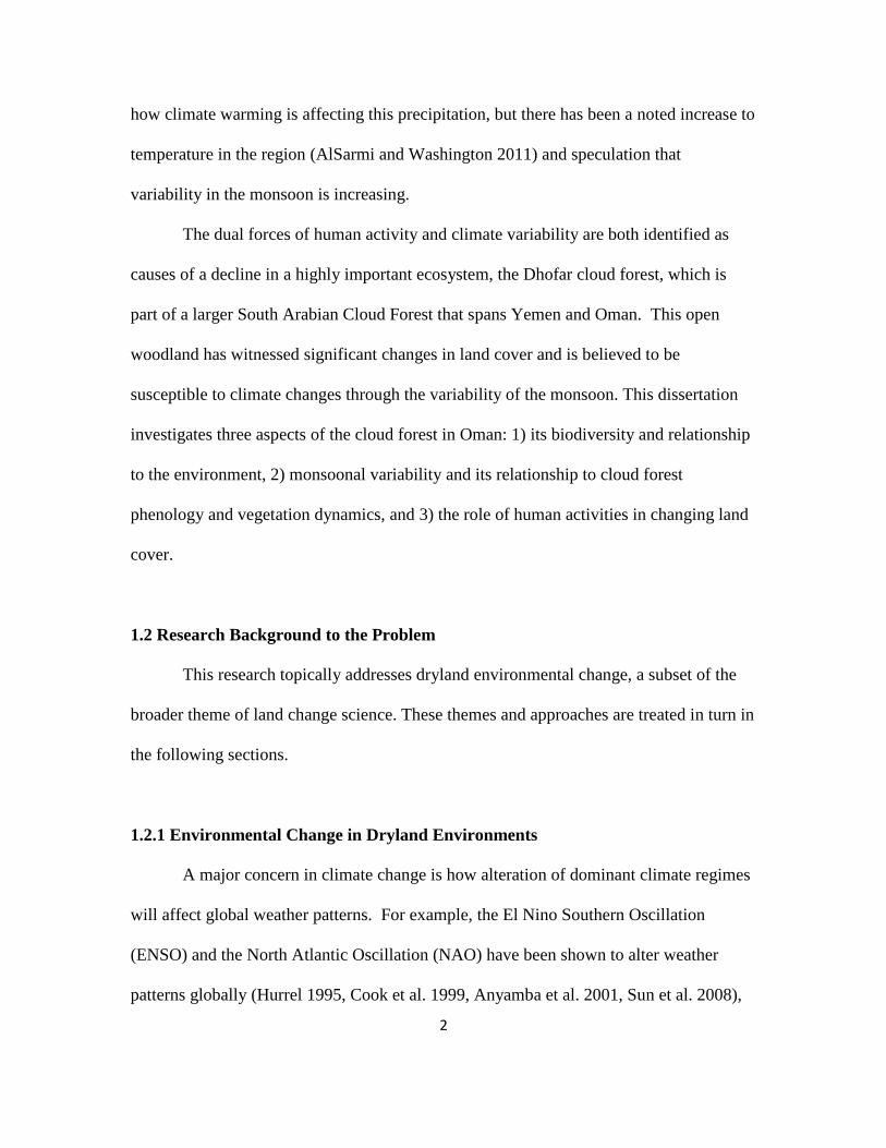
how climate warming is affecting this precipitation, but there has been a noted increase to
temperature in the region (AlSarmi and Washington 2011) and speculation that
variability in the monsoon is increasing.
The dual forces of human activity and climate variability are both identified as
causes of a decline in a highly important ecosystem, the Dhofar cloud forest, which is
part of a larger South Arabian Cloud Forest that spans Yemen and Oman. This open
woodland has witnessed significant changes in land cover and is believed to be
susceptible to climate changes through the variability of the monsoon. This dissertation
investigates three aspects of the cloud forest in Oman: 1) its biodiversity and relationship
to the environment, 2) monsoonal variability and its relationship to cloud forest
phenology and vegetation dynamics, and 3) the role of human activities in changing land
cover.
1.2 Research Background to the Problem
This research topically addresses dryland environmental change, a subset of the
broader theme of land change science. These themes and approaches are treated in turn in
the following sections.
1.2.1 Environmental Change in Dryland Environments
A major concern in climate change is how alteration of dominant climate regimes
will affect global weather patterns. For example, the El Nino Southern Oscillation
(ENSO) and the North Atlantic Oscillation (NAO) have been shown to alter weather
patterns globally (Hurrel 1995, Cook et al. 1999, Anyamba et al. 2001, Sun et al. 2008),
3
primarily through teleconnections. The ENSO can affect ecosystems throughout Africa,
North America, and the Indian Ocean (Cook et al. 1999, Anyamba et al. 2001, Kumar et
al. 2006). In the deep past, monsoonal winds, as measured from Arabian Sea cores, have
been shown to correlate with ice-rafted debris in the North Atlantic, as affected by the
NAO (Anderson et al. 2002). In either case, the ENSO and NAO are measured by
indices, and these indices can be compared to local climate data to predict how climate
anomalies associated with these regimes will affect temperature and precipitation in local
regions (e.g. Pozo-Vazquez et al. 2001).
Aridification or desertification is not only a product of climate oscillations, but of
inappropriate human use of drylands (Reynolds and Stafford-Smith 2002).
Understanding their relative roles is often a vexing issue. Several examples, illustrate this
problem. The 1930s Dust Bowl in the southern Great Plains of the United States has long
been identified as climatic drought affecting inadequate farming practices. Recent
modeling work, however, indicates that such a large magnitude drought in the center of
the U.S. involved feedbacks between large-scale land clearing and poor farming practices
(Cook et al 2009). Decades (1960s-80s) of drought in the Sahel of Africa were attributed
to land degradation from cropping and grazing (Fairhead and Leach 1986, Reynolds and
Stafford-Smith 2002). Human-induced land degradation was called into question when a
recovery of the Sahel was instigated by a change in sea surface temperature in the
Atlantic Ocean during the 1990's (Hulme 2001). Local human-induced environmental
impacts notwithstanding, the large aridification of the Sahel was largely climatic in origin
(Nicholson 1993, Nicholson 2009) with localized impacts related to land uses. Finally,
comparisons of human and environmental responses to drought cycles, stocking, land

4
management decisions, and institutional action in Australia demonstrates how land
management decisions to continue high stocking rates, despite decreasing biomass,
amplified land degradation in the outback in the face of drought (Stafford-Smith et al.
2007). These examples highlight the critical role of an integrated analysis of the coupled
human environment system, but it also highlights how human actions and institutional
policies can be just as formidable for land change as the climate.
1.2.2 Land Change Science
Land change or land system science (LCS) examines human-environment
interactions on ecosystem and human wellbeing (Turner, Lambin, and Reenberg 2007).
It does so through monitoring and observation, coupled human-environment analysis,
modeling, and synthesis. Observations and monitoring of the human environment often
use remote sensing to measure change. A variety of platforms and technologies have
enabled multi-decadal monitoring of the Earth system. In general, there are three scales
used for Earth observation: high, medium, and low resolution. High-resolution imagery
can provide fine scale monitoring, between 1 and 15 m, and is often used for cross-
sectional snapshots of the environment (e.g. Walsh and et al. 2008a,b). Perhaps the most
common sensors employed for large-area studies of land change, however, are medium
resolution imagery, such as Landsat, which has a 30 m resolution (e.g., Gutman et al.
2004). MODIS, another important platform, is a low resolution sensor (compared to
Landsat) capable of capturing Earth observations between 250 m and 1 km in resolution,
but it has the capability of generating snapshots of vegetation, surface temperature, and
albedo every eight to sixteen days, making its temporal resolution nearly unmatched by
5
other sensors (Justice et al. 1998). It is increasingly common to combine data from
multiple sensors to understand land change.
Regardless of the sensor, land-use/cover maps can be generated from classified
images. Biophysical variables can also be quantified directly, for example: NDVI,
temperature, albedo, emissivity, and evapotranspiration. Finally, the form of the land can
be discerned as well, usually from configuration metrics derived from classified images
(Turner 1989). Human and environmental subsystems are inherently complex, elevating
the usefulness of modeling as a tool to combine observations from remote sensing with
biophysical impacts/feedbacks and land-use change drivers (NRC 2014). Common
modeling methods in LCS include, among many others, agent based models (ABM) and
economic models. ABM’s simulate a process using various software agents to mimic
real world behavior. They can incorporate socioeconomic data, environmental data from
remote sensing, and lab data (Manson and Evans 2007). Economic models of land change
attempt to capture key characteristics of behavior that lead to certain land change
outcomes. Regression models are common (e.g. Southgate et al. 2009) where conceptual
models of a dependent land change outcome variable are tested for correlation with a
variety of possible drivers (the independent variables). No matter the type of model used,
the process of modeling in LCS is useful for linking the socioeconomic drivers with
biophysical outcomes and feedbacks.
An ongoing problem has been to link the land change observed in remote sensing
with the socioeconomic drivers of change, in part because these drivers are arrayed along
a proximate to distal axis. The direct or immediate drivers are easy to identify and
associate quantitatively to land change. Typically the more distal the driver, the more
6
difficult it is to demonstrate such associations. To this end, synthesis in LCS has focused
on uncovering the socioeconomic drivers that may be complex and masked from direct
observation (Lambin et al. 2001; Seto and Reenberg 2014). In Vietnam, for example,
reforestation is prevalent despite a large internal demand for wood. In this case, wood is
imported to serve demand, while regenerating local forests (Meyfroidt and Lambin
2009). Whether direct or indirect, globalization is a persistent force affecting land cover
change around the world (Liu et al. 2013, Meyfroidt and Lambin 2009, Seto and
Reenberg forthcoming). Access to markets creates complexity and price vulnerabilities,
and along with economic fluctuations from globalization causes uncertainty (Defries et
al. 2010). LCS and global change studies show that environmental change is a complex
process. Distal influences can be attributed to changes in population, technology,
urbanization, institutions, and globalization (Turner and Robbins 2008, Brannstrom and
Vadjunec 2014, Seto and Reenberg 2014). These four aspects place pressure on human
environment systems, which affects ecosystem services through the supply and demand
of industrial goods and services. Globalization seems to be the common distal factor at
the heart of land change (Lambin et al 2001), but population, technology, institutions, and
urbanization play an important role as conduits for the demand of resources and
ecosystem services, and seem to be at the heart of wider changes taking place in the
global environment, including anthropogenic climate change (Liu et al. 2013).
1.2.3 Quantifying Environmental Change
Two common methods for analysis of remotely sensed images, and the methods
that are used here, are the subpixel method and time series analysis. The subpixel

7
approach offers an understanding of how land covers fractionally occupy a pixel. Time
series analysis is suitable for understanding the role that climate plays on environmental
features, such as phenology and teleconnections.
1.2.4 Subpixel Approach
Ground covers that occupy varying proportions of the landscape can be extracted
from the pixel by assuming that each pixel comprises a combination of all possible
ground covers in the scene (Settle and Drake 1993). Generally, the classic approach to
finding endmember combinations is known as the linear mixture model or as spectral
mixture analysis (SMA; Settle and Drake 1993). To achieve understanding of what
ground covers occupy a pixel each pixel is considered to be a linear combination of
differing endmembers, which is denoted mathematically as,
𝓍 = ∑ 𝑓𝑖𝑃𝑖𝜆 + 𝜖
𝑛
𝑖=1
(1)
where 𝓍 is the scene pixel, 𝑛 is the number of endmembers, 𝑓𝑖 is the fraction of the pixel
occupied by that endmember, 𝑃𝑖𝜆 represents the reflectance values of the endmember at
each band λ, and 𝜖 is an error term. One constraint is usually imposed on the model,
∑ 𝑓𝑖 = 1
𝑛
𝑖=1
(2)
This constraint ensures that no combination of endmembers occupies more than 100% of
the pixel. Modeling of the pixels requires training data taken within the image scene or
some measured reflectance for each endmember 𝑛. Measured reflectance values can
come from spectrometer readings or one of many published spectral libraries, and usually

8
are taken without atmospheric conditions or disturbance. Training data are usually
preferred because even when an image is converted to reflectance, the atmospherically
corrected scenes are usually not absolutely correct, which can obscure the results.
Training data are therefore preferable because the pixel's reflectance values are
adequately drawn from within the image along with any noise inherent within the image.
There are some limitations to using SMA. First, the number of endmembers
cannot exceed the number of bands plus one (Settle and Drake 1993). In a Landsat 5 TM
image with six visible and near infrared bands only seven endmembers can be modeled.
This restriction of endmembers in the scene may not represent reality, especially for a
heterogeneous image with a great number of different land covers. Second, endmembers
and their training data must be chosen to be as close as possible to the reflectance values
of the land cover or class being modeled, therefore the selection of training data is critical
(e.g. Dawelbait and Morari 2012).
One improvement to the SMA that addresses some of the limitations with the
classic approach is multiple endmember spectral mixture analysis (MESMA). MESMA
was developed as a way to address the limitation in SMA that requires that all
endmembers of interest be modeled at every pixel (Roberts et al. 1998). This approach
allows the number and type of endmembers to vary from one pixel to the next.
Endmembers can be selected from spectra measured in the field or laboratory, or selected
from within the image. Models are selected by using the model with the minimum root
mean square error (RMSE). RMSE is defined as,
𝑅𝑀𝑆𝐸 = √∑ (𝜖𝑖)2𝜆
𝑖=1
𝑁 (3)
9
N is the number of reference endmembers. The RMSE measures the residual error of a
subpixel estimator. Fractions are also allowed to vary between -0.01 and 1.01. The
benefits of using this approach are that endmembers can be modeled as two or more
endmember models. For example, MESMA has been used to model vegetation, soil,
shade, and senesced grass in the Santa Ynez Mountains of California and other
environments, and has been effective in mapping subpixel fractions (Dennison and
Roberts 2003).
1.2.5 Time Series Analysis
Whether using a subpixel approach or a pixel based approach, imagery can be
coupled with time series analysis to measure environmental change. Researchers have
noted that high temporal resolution studies are most likely best for uncovering the effects
of climate variability and anthropogenic changes. Lambin and Linderman (2006) point
out that the most common data for studying land change are generally higher spatial,
lower temporal resolution satellites. Land-cover conversions, like deforestation, can be
ideally studied with these types of data because changes to the tree cover fluctuate less
than the temporal coverage of the satellite. However, land-cover alterations, such as
degradation of pastures on grasslands, might not be as easily detectable because they
differ from one year to the next, and sometimes within the same year. Land-cover
alteration is the absence of a conversion of one land-cover type to another. Alteration
through degradation might result in a lower overall net primary production, but the land
cover will still remain grass.
10
A variety of methods have been used to circumvent the problem in land-cover
alteration. One way to measure these alterations (in this case, overgrazing) is to use a
linear correction of NDVI values over a study period to compensate for rainfall
variability (Archer 2004). Another important technique is time series analysis of
remotely sensed images, particularly for phenology analysis, which is the study of the
greening period of vegetation. Phenology analysis is associated with a peak in the
growing season and then the senescence of the vegetation to an annual minimum during a
yearly cycle (de Beurs and Henebry 2010). While phenology can be estimated with a
number of different techniques, satellites can make the task of estimating phenology
parameters easy by compiling a time series of NDVI rasters, preferably of high temporal
resolution (such as monthly or every 16 days). Once a high temporal resolution of NDVI
images is compiled, a trend can be estimated. Calculating trends can include a linear
regression of the time series or some non-parametric calculation of the trend line. Non-
parametric trends are often considered to be advantageous because they are not reliant on
certain statistical assumptions. Panday and Ghamire (2012) used a seasonal trend
analysis to assess NDVI time series over the Hindu-Kush region of the Himalayas
between 1982 and 2006. The NDVI data were first processed using a harmonic
regression, which fits a curve to the data (Eastman et al. 2009). Once the harmonic
regression was applied, they analyzed three aspects of the data for trends: Amplitude 0,
Amplitude 1, and Phase 1 (Eastman et al. 2009; 2013). Amplitude 0 is the average
annual NDVI value. Amplitude 1 is the magnitude of the peak NDVI value over a year
while considering the minimum as well. Phase 1 represents the timing of the maximum
NDVI value at a pixel; an assessment of the Phase 1 signal gives the timing of the
11
greening cycle. A trend assessment algorithm can then be used to determine the slope of
a trend and its significance for these three parameters (Eastman et al. 2009; Neeti and
Eastman 2012). A common way to derive a trend slope is by using a Theil-Sen median
slope, which is a non-parametric technique that performs a pair-wise comparison of time
series observations in the NDVI images (Theil 1950; Sen 1968). Finally, the significance
of the Theil-Sen median slope is assessed using a Man Kendall test to detect whether the
trend is significantly increasing or decreasing monotonically (Mann 1945).
1.3. Research Problems and Questions
1.3.1 Study Area & Problem Specification
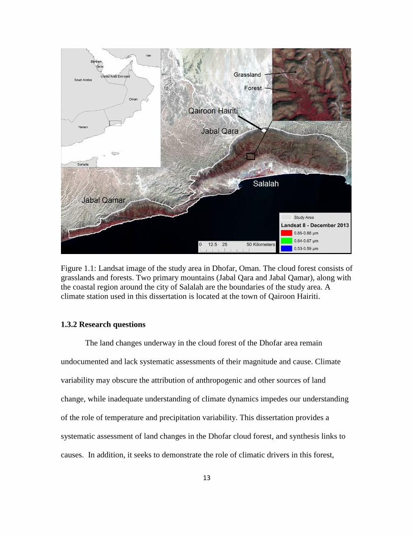
The study area for this dissertation is the Dhofar portion of the South Arabian
Cloud Forest, also known as the Dhofar cloud forest (Figure 1.1). The South Arabian
Cloud Forest is a deciduous, seasonal forest (Hildebrandt 2005) that exists in fragments
along the southern coast of Oman and Yemen. Two mountains are the primary focus
throughout this dissertation, Jabal Qara and Jabal Qamar, both of which are in Dhofar,
Oman, and house the largest potions of the cloud forest. The cloud forest, thought to be
the native home of frankincense (Boswellia sacra), is comprised mainly of broadleaf tree
species (Kurschner et al 2004) and grasslands. The Indian Summer Monsoon (ISM)
provides the essential precipitation that supports the ecosystem and gives the region its
unique, oasis-like landscape.
The start and end of the ISM (known locally in Arabic as khareef) as well as the
intensity of the winds varies by year (Anderson et al. 2002, Goswami and Mohan 2001,
Gupta et al. 2003, Kumar et al. 2006, Scholte et al. 2010). Khareef is generated when a
12
summer upwelling of cold water in the Indian Ocean creates cloud fog that pushes against
the Dhofar Mountain range for about three months, from approximately the end of June
to the beginning of September. Horizontal precipitation from the summer clouds
provides light drizzle and substantial cloud moisture (Hildebrandt 2005, Hildebrandt and
Eltahir 2006, Hildebrandt and Eltahir 2007). Dense vegetation grows in direct contrast to
the more arid lands located to the north of the cloud forest. From what is known about
the timing and intensity of the ISM in other parts of the Indian Ocean, the beginning and
ending, as well as the intensity of the ISM can vary from one season to the next.
The cloud forest provides ecosystem services that are essential to local
livelihoods, including ecotourism, biomass production for rangelands, amongst others
(e.g. frankincense extraction, wood harvesting, water provisioning). Numerous factors
have raised concerns regarding land-use and land-cover change in the forest. First, camel
and bovine grazing on the cloud forest's rangelands are thought to have caused
degradation of the grasslands as well as a reduction in tree density (Hildebrandt and
Eltahir 2006). Second, modernization, supported by global demand for Oman's modest
oil reserves have encouraged infrastructure development, such as roads and buildings for
new settlements, as well as the growth of Salalah, the nearby city, that may indirectly
affect the cloud forest.
13
Figure 1.1: Landsat image of the study area in Dhofar, Oman. The cloud forest consists of
grasslands and forests. Two primary mountains (Jabal Qara and Jabal Qamar), along with
the coastal region around the city of Salalah are the boundaries of the study area. A
climate station used in this dissertation is located at the town of Qairoon Hairiti.
1.3.2 Research questions
The land changes underway in the cloud forest of the Dhofar area remain
undocumented and lack systematic assessments of their magnitude and cause. Climate
variability may obscure the attribution of anthropogenic and other sources of land
change, while inadequate understanding of climate dynamics impedes our understanding
of the role of temperature and precipitation variability. This dissertation provides a
systematic assessment of land changes in the Dhofar cloud forest, and synthesis links to
causes. In addition, it seeks to demonstrate the role of climatic drivers in this forest,

14
focusing on the delineation of their relative roles and the consequences to phenology.
These general queries are addressed through a specific set of questions asked about the
study site.
1. What is the annual variability in monsoon conditions in the Dhofar cloud forest,
and how can this variability be quantified using climate and remote sensing data?
2. How sensitive is the phenology of the Dhofar cloud forest to variability of the
monsoon and oscillations in climate teleconnections?
3. What is the distribution of trees and shrubs across the Dhofar cloud forest?
4. What is the trend in NDVI over the last 13 years? How does this trend relate to
deforestation, overgrazing, and the built environment?
5. What land changes have occurred between 1970 and today? What are the causes?
1.4 Organization of Dissertation
This dissertation incorporates three types of analyses organized in three studies
(research papers) to investigate the relative roles of climate and anthropogenic influences
in shaping the environment in Dhofar, Oman. Each paper, the data (see also Table 1.1),
and analyses are noted below.

15
Table 1.1: Datasets used in this dissertation Data Category Data Set Description Time Frame
Climate Temperature Daily and monthly averages. Time
series. Stations: Qairoon Hairiti
2001-2013
(QH)
Precipitation Daily and monthly averages. Time
series. Stations: Qairoon Hairiti
2001-2013
(QH)
Reanalysis II Forecasted climate variables used to
understand the timing of the monsoon
1979-2013
Environment NDVI 16 day MODIS time series 2001-2013
Slope Derived from elevation 1999
Aspect Derived from elevation 1999
Hydrology Derived from elevation 1999
Elevation Meters above sea level; from Shuttle
Radar Topography Mission
1999
Tree and shrub survey
data
Primary data collected during survey.
Includes the density, frequency, and
cover of dominant species
2013
Land cover/use Built environment Derived from Landsat 5-8 1988 and 2013
Forest (trees) Derived from Landsat 5-8 1988 and 2013
Grassland Derived from Landsat 5-8 1988 and 2013
Shrubs Derived from Landsat 5-8 1988 and 2013
Agriculture Derived from Landsat 5-8 1988 and 2013
Coastal alluvium Derived from Landsat 5-8 1988 and 2013
Desert gravel plains Derived from Landsat 5-8 1988 and 2013
Water Derived from Landsat 5-8 1988 and 2013
Impervious surfaces
(roads)
Derived from Landsat 5-8 1988 and 2013
1.4.1 Indian Ocean Monsoon Dynamics in Southern Arabia and Effects on the
Vegetation Phenology of a Seasonal Cloud Forest
Chapter 2 identifies correlations between the climate dynamics of the southern
Arabian Peninsula and the Dhofar cloud forest. Comparisons are drawn between yearly
monsoonal precipitation, monsoon timing, and temperature with seasonal parameters of
cloud forest vegetation.
Precipitation data were collected at Qairoon Hairiti (in the Dhofar cloud forest,
see Figure 1.1), while temperature data came from Reanalysis II (NOAA; Kanamitsu et
al. 2002). Time series of climate regimes were constructed from data addressing three
16
climate phenomena: the Indian Ocean Dipole (IOD), ENSO, and sea surface temperatures
(SST). These three phenomena have been shown to influence weather and climate near
the Arabian Peninsula. To measure the impact of these three climate phenomena,
correlations are drawn between their index series and seasonal parameters for the cloud
forest. Mean annual NDVI (Amplitude 0), magnitude of the peak NDVI signal
(Amplitude 1), and timing of peak greenness (Phase 1) were extracted for the Dhofar
Cloud forest using the Earth Trends Modeler in Idrisi.
Correlation between time series and the relationship between phenology and
climate are derived using linear models from the Earth Trends Modeler in Idrisi. Linear
models in time series analysis are analogous to those from linear regression. Common
metrics for evaluating the model, such as the slope, intercept, coefficients, R2, and
residuals, are used to assess the correlation between climate indices (SST, IOD and
ENSO). The purpose of this analysis is to measure how much influence the various
climate regimes have on local Dhofar climate and cloud forest phenology, which is
important for understanding the vulnerability from global climate change and tipping
elements in the Earth system (Lenton et al. 2008).
The start and end of the Indian Ocean Monsoon is developed in two models. The
first model is based on maximum daily temperature data from Reanalysis II (Kanamitsu
et al. 2002) for the period 1979 to 2013. The second model constructs the start and end of
the monsoon using cloud cover data from 2001 to 2013 using MODIS daily images.
Average values of the MODIS band-4 reflectance are used to measure cloud cover over
the study area. The timing and length of the monsoon are compared with MODIS NDVI

17
time series and sum NDVI values for October to December (Wessels and colleagues
2012).
A Theil-Sen median trend was used to estimate changes in NDVI between 2001
and 2013 (Theil 1950, Sen 1968). The identification of trends provides insight into
conditions for increased or decreased biomass production. These climate trends are
compared to cloud forest NDVI trends at 12 random sites.
1.4.2 Drivers of Plant Diversity in the South Arabian Cloud Forest
The primary goal of Chapter 3 is to understand mechanisms that drive
biodiversity in the Dhofar cloud forest. A floral survey is conducted to measure
biodiversity and to understand the mechanisms of biodiversity patterns.
Three measurements—density, cover, and frequency (Mitchell 2007)—were
taken for 102 randomly selected surveyed plots. The importance value of a species was
calculated and mapped for all plots, providing a geographic distribution of the principal
species and to help define the various ecological communities.
In addition to importance value, biodiversity indices were calculated from the
vegetation data. The diversity measurements were used to determine biodiversity
patterns.
Finally, assessment of the distribution of species and biodiversity hotspots of the
tree and shrub species surveyed constitute two distinct sub-analyses: those within the
cloud forest proper and those within the plateau grasslands. Chapter 2 tests several
hypotheses about biodiversity patterns and uses a cluster analysis to define the vegetation
communities. The floral analysis includes many environmental variables (e.g., slope,
18
elevation, hydrology, aspect), climate variables (precipitation and temperature), as well as
anthropogenic variables (e.g., distance to roads, and distance to buildings).
1.4.3 Land Changes and their Drivers in the Dhofar, Oman Cloud Forest and
Coastal Zone between 1988 and 2013
Chapter 2 and 3 improve understanding of how the climate has affected the
overall ecosystem of the cloud forest, biogeography of the cloud forest, and crucial areas
of biodiversity that are susceptible to human impacts and variable climate. Chapter 4
quantifies the changes in land covers and uses in Dhofar's cloud forest and the adjacent
coastal zone and associates these changes to various drivers of change.
Land change is quantified between 1988 and 2013. The first year captures the
beginning of major socioeconomic changes in Oman, registered by the growth of Salalah.
The land-cover categories addressed are trees, grasses, shrubs, agriculture, coastal
alluvium, desert gravel plains, water, roads, and built environment. These categories
included the major land-covers observed in the cloud forest zone and the lands
surrounding the forest. Special attention is given to the identification of overgrazing and
deforestation (i.e., forest thinning). Change analysis is conducted with Idrisi Land
Change Modeler (LCM). LCM analyzes land-cover images to determine areas of change
and provide transition areas and prediction of change. Additionally, a sub-pixel analysis
measures the shifts in forest fractions (i.e., thinning) between 1988 and 2013.

19
CHAPTER 2
AN ASSESSMENT OF MONSOON TIMING, CLIMATE REGIMES, AND
MONSOON VARIABILITY ON VEGETATION DYNAMICS IN SOUTHERN
ARABIA
2.1 Abstract
The Indian Summer Monsoon (ISM) is critical for vegetation in southern Arabia,
particularly for the drought deciduous cloud forest in the Dhofar region of Oman. This
paper investigates two potential influences of variance or changes in the ISM on the
vegetation dynamics in the cloud forest. The first involves the relationship between
monsoon variability and timing, and seasonal vegetation. The second addresses the
correlation between normalized difference vegetation index (NDVI) time series, acquired
from MODIS satellite imagery, and climate systems, such as El Niño Southern
Oscillation (ENSO), Indian Ocean Dipole (IOD), and sea surface temperatures (SST) in
the Arabian Sea. Additionally, timing of the monsoon was modeled using Reanalysis II
data and daily satellite images from MODIS.
The findings reveal that the seasonal vegetation parameters are resistant to
variability in measureable precipitation, monsoon length, and temperature. The strongest
correlations were found with June precipitation and temperature, but these were generally
weak to moderate explanations of the variance. Even broader climate regimes, such as
ENSO and IOD, show weak to no correlation with NDVI time series. Cloud forest
phenology shows a stronger correlation to SST in the Arabian Sea, with SST about six to

20
nine months out of phase with NDVI time series (SST leading). The evidence, therefore,
suggests that the cloud forest is resilient in the face of climate change.
2.2 Introduction
The Indian Summer Monsoon (ISM; henceforth, monsoon) is foundational for the
vegetation of the Southern Arabian Peninsula. Known locally as khareef, the monsoon is
responsible for most of the precipitation in the southern region of Oman, or Dhofar, as
well as parts of Yemen. Monsoon precipitation supports the ecosystem of the Dhofar
Mountains, where a drought deciduous cloud forest thrives in those parts of the
mountains near the coast (Hildebrandt and Eltahir 2006). This cloud forest, part of the
South Arabian Cloud Forest, is one of the most diverse ecosystems in the peninsula
(Miller and Morris 1988; Ghazanfar and Fisher 1998).
The ISM reliably develops over the Arabian Sea in late May and early June of
each year (Fieux and Stommel 1977; Joseph et al. 1994; Fasullo and Webster 2003;
Joseph et al. 2006). In general, warmer terrestrial air masses meet cooler ocean air masses
caused by upwelling off the coast of the Arabian Peninsula. As these two air masses
meet, clouds form along southern part of the peninsula. The clouds arrive several weeks
after the ISM winds develop out of the southwest and are responsible for the highest
period of precipitation.
Several studies demonstrate that the monsoon delivered more rainfall in past
pluvial periods over the southern Arabian Peninsula (Fleitmann et al. 2003; Fleitmann et
al. 2004; Blechschmidt et al. 2009; Cremaschi and Negrino 2005; Fleitmann and Matter
2009; Fleitmann et al. 2011). These studies link increased rainfall to warming during
21
peak interglacial periods, such as the Early Holocene and the Last Interglacial, and were
driven by changes in the Intertropical Convergence Zone (ITCZ) and minimal Arctic sea
ice extent (Overpeck et al. 1996; Fleitmann and Matter 2009). The effects of current
anthropogenic climate change on monsoon rainfall are largely unknown. There is some
indication that monsoon rainfall in India changed in the latter part of the 20th century,
leading to a significant reduction in moderate and heavy rainfall days owing to a
weakening monsoon circulation pattern (Krishnan et al., 2013). Climate model
simulations suggest that global warming has the potential to destabilize the monsoon
even further (Krishnan et al. 2013). Recent warming across the Arabian Peninsula
(AlSarmi and Washington 2011), perhaps linked to anthropogenic climate change (IPCC
2014), has sparked interest in the study of the monsoon, with attention to vulnerabilities
to its stability and impacts on vegetation. Some evidence points to a decreasing trend in
rainfall, but results are not necessarily significant statistically (Kwarteng et al. 2009;
AlSarmi and Washington 2011). At least one study did find significant results indicating
decreasing July and August precipitation trends over Salalah in Dhofar, Oman (AlSarmi
and Washington 2011). The consequences of this decrease for the cloud forest vegetation
are not well understood, mainly because time series analyses of vegetation dynamics and
climate variability have not been worked out.
Broader climate factors and their effects on the cloud forest are another area of
emerging interest. The Indian Ocean Dipole (IOD), an oscillation of sea surface
temperatures in the eastern and western parts of the Indian Ocean, is one such factor (Saji
et al. 1999). Positive and negative modes of the IOD have been correlated to droughts
and floods in Africa, Australia, and Indonesia, and they may affect the ISM (Ashok et al.
22
2001, 2004). The El Niño Southern Oscillation (ENSO) may also affect the ISM, though
the relationship is thought to be indirect (Charabi 2009).
This paper provides new evidence and analysis directed to the question of ISM
variability and vegetation consequences for the Dhofar cloud forest of Oman. It explores
the timing of the monsoon using satellite imagery and climate data from ground stations
and Reanalysis 2. In addition, it explores how monsoon variability and other climate
factors may influence vegetation dynamics in the cloud forest using a time series of
satellite images. In the process, this study
models the timing of the monsoon in southeast Arabia;
describes the characteristics of the cloud forest’s phenology;
determines the sensitivity of vegetation dynamics to climate variability; and,
determines the relationship between broader climate factors and cloud forest
dynamics.
2.3 Study Area
The study area includes the southern portions of the Arabian Peninsula and the
South Arabian Cloud Forest in Dhofar, Oman. Also addressed are the broader climate
patterns for the monsoon across southeastern Arabia and the Arabian Sea. Vegetation
patterns and phenology are restricted to the cloud forest in Dhofar, Oman.
The cloud forest occupies the mountain range in Dhofar (Figure 1.1). Three
primary mountains comprise the range: Jabal Qara, Jabal Qamar, and Jabal Samhan. The
cloud forest is primarily situated in Jabal Qara and Jabal Qamar, but a small section runs
along the cliffs of Jabal Samhan.
23
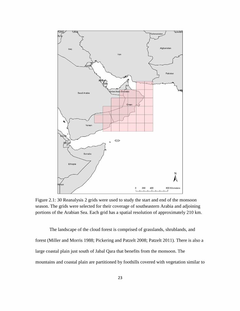
Figure 2.1: 30 Reanalysis 2 grids were used to study the start and end of the monsoon
season. The grids were selected for their coverage of southeastern Arabia and adjoining
portions of the Arabian Sea. Each grid has a spatial resolution of approximately 210 km.
The landscape of the cloud forest is comprised of grasslands, shrublands, and
forest (Miller and Morris 1988; Pickering and Patzelt 2008; Patzelt 2011). There is also a
large coastal plain just south of Jabal Qara that benefits from the monsoon. The
mountains and coastal plain are partitioned by foothills covered with vegetation similar to
24
that found in the cloud forest. Approximately 29% of the cloud forest and coastal plain
has tree cover, the rest is a mix of grasslands and shrublands. Because this region is one
of the few areas on the Arabian Peninsula to have dense vegetation, grazing is heavy and
animal husbandry is widespread. Cattle, camels, and goats are the primary livestock and
are important sources of subsistence for the people living in the Dhofar Mountains
(Janzen 1986; 2000).
The vegetation reaches peak biomass during the monsoon and senesces several
months after the monsoon fog subsides (Hildebrandt and Eltahir 2006). Forested areas are
descended from an ancient forest that once stretched from India to Africa during the
Tertiary period (Kürschner et al. 2004). Current vegetation is associated with the Saharo-
Sindian and Saharo-Arabian phytogeographic zones (Ghazanfar and Fisher 1998; Parker
and Rose 2008).
The yearly temperature range for the cloud forest can vary from mean minimum
temperatures of 19° C in January to mean maximum temperatures around 32.5° C in June
(Galletti forthcoming). Daily average temperatures are less than 25° C during monsoon
months. Mean annual precipitation normally measures around 200 mm. Monsoon
precipitation on average accounts for more than 100 mm a year. The driest months are
usually November, December, and January, when precipitation is less than 10 mm on
average.
25
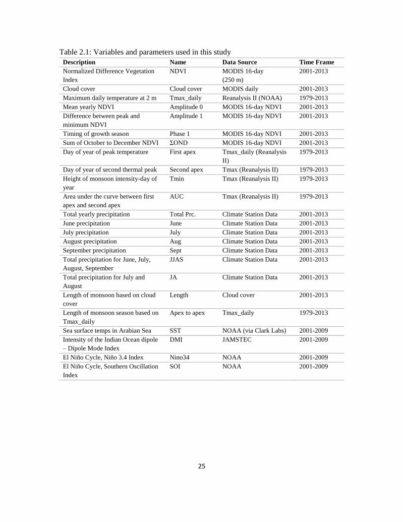
Table 2.1: Variables and parameters used in this study
Description Name Data Source Time Frame
Normalized Difference Vegetation
Index
NDVI MODIS 16-day
(250 m)
2001-2013
Cloud cover Cloud cover MODIS daily 2001-2013
Maximum daily temperature at 2 m Tmax_daily Reanalysis II (NOAA) 1979-2013
Mean yearly NDVI Amplitude 0 MODIS 16-day NDVI 2001-2013
Difference between peak and
minimum NDVI
Amplitude 1 MODIS 16-day NDVI 2001-2013
Timing of growth season Phase 1 MODIS 16-day NDVI 2001-2013
Sum of October to December NDVI ΣOND MODIS 16-day NDVI 2001-2013
Day of year of peak temperature First apex Tmax_daily (Reanalysis
II)
1979-2013
Day of year of second thermal peak Second apex Tmax (Reanalysis II) 1979-2013
Height of monsoon intensity-day of
year
Tmin Tmax (Reanalysis II) 1979-2013
Area under the curve between first
apex and second apex
AUC Tmax (Reanalysis II) 1979-2013
Total yearly precipitation Total Prc. Climate Station Data 2001-2013
June precipitation June Climate Station Data 2001-2013
July precipitation July Climate Station Data 2001-2013
August precipitation Aug Climate Station Data 2001-2013
September precipitation Sept Climate Station Data 2001-2013
Total precipitation for June, July,
August, September
JJAS Climate Station Data 2001-2013
Total precipitation for July and
August
JA Climate Station Data 2001-2013
Length of monsoon based on cloud
cover
Length Cloud cover 2001-2013
Length of monsoon season based on
Tmax_daily
Apex to apex Tmax_daily 1979-2013
Sea surface temps in Arabian Sea SST NOAA (via Clark Labs) 2001-2009
Intensity of the Indian Ocean dipole
– Dipole Mode Index
DMI JAMSTEC 2001-2009
El Niño Cycle, Niño 3.4 Index Nino34 NOAA 2001-2009
El Niño Cycle, Southern Oscillation
Index
SOI NOAA 2001-2009

26
2.4 Data and Methods
2.4.1 Climate, Monsoon Timing, and Analysis
Table 2.1 lists the variables used in this study, a combination of observed and
modeled data, as well as measures derived from them. Two separate models were
developed to study the onset and withdrawal of the monsoon. The first model is based on
temperature data, and the second, on observations of cloud cover.
The first model of the monsoon was developed using Reanalysis 2 data
(Kanamitsu et al. 2002) for the period 1979-2013 over 30 grids covering southeast Arabia
and the Arabian Sea (Figure 2.1). Two meter maximum daily temperature was used to
define the monsoon season by fitting a curve to the daily temperature observations using
a polynomial regression (based on a 15th order polynomial). The polynomial curve was
fitted to each year between 1979 and 2013. Temperature maxima and minima were
extracted for each year and provide the monsoon seasonal parameters used to estimate the
timing of the monsoon.
Moderate Resolution Imaging Spectroradiometer (MODIS; Justice et al. 1998)
imagery was used to observe daily cloud cover and estimate the temporal dynamics of the
monsoon. MODIS daily images from 2001 to 2013 were visually analyzed to measure the
timing of consistent cloud cover over the study area. Three days of continuous cloud
cover observed in June or July with no breaks in cloud cover for more than two days was
used to establish the onset of the monsoon as experienced on the ground. The end of the
monsoon was registered by three consecutive cloud-free days after the end of August.
In addition to the monsoon models, several climate variables were estimated using
climate station data from Qairoon Hairiti, located within the cloud forest. Table 1 lists
27
these variables, which are mostly combinations of precipitation accumulation for the
monsoon months or precipitation for an individual month.
2.4.2 Vegetation Data and Analysis
MODIS was used to obtain time series data of NDVI for the study area. MODIS
creates a composite NDVI image every 16-days based on the highest NDVI value
observed for a pixel at resolution is 250 m (Justice et al. 1998), which results in 23
composite images per year. MODIS images were collected for the period 2001-2013.
Analysis of vegetation data includes the creation of bivariate linear models to
explore relationships between vegetation patterns and broader climate regimes. These
models use the MODIS NDVI data as a dependent variable; climate indices and SST
monthly data are used as explanatory variables. Sixteen-day MODIS data were
transformed to monthly averages (to fit the data measurements of the climate indices).
The four climate indices were: Niño 3.4 index (an index of the El Niño Southern
Oscillation [ENSO] based on SST models [Rayner et al. 2003]); the Southern Oscillation
Index (SOI; another index of ENSO [Trenberth 1984]); the Dipole Mode Index (DMI; an
index of the IOD based on SST differentials between the east and west Indian Ocean
[Saji et al. 1999]); and SST in the Arabian Sea. The Niño 3.4 and SOI datasets were
obtained from NOAA NCDC. The SST data were obtained for the years of 1982 to 2009
from Clark Labs, which was based on a NOAA AVHRR dataset (Reynolds et al. 2002).
These bivariate analyses are based on the period 2001-2009 when all climate, SST, and
NDVI observations are aligned.
28
2.4.3 Seasonal Parameters of Vegetation
Seasonal vegetation variables were estimated using methods from Eastman and
associates (2009; 2013). Mean annual NDVI (Amplitude 0), NDVI annual cycle
(Amplitude 1), timing of the peak annual NDVI cycle (Phase 1), and sum of the NDVI
for October to December (ΣOND) were derived from MODIS 16-day NDVI composite
images. Amplitude 1 is calculated by taking the difference between the maximum and
minimum values of a modeled NDVI curve (Eastman et al. 2013). Amplitude 0 is the
mean annual NDVI. Phase 1 is the timing of the peak of the annual cycle. ΣOND is
derived by summing all 16-day composite images for October to December of each year.
ΣOND is a useful parameter because it measures the sum NDVI of the study area right
before senescence and during months that have very low cloud cover. Phase 1, Amplitude
0, and Amplitude 1 are derived from curves that are fitted to the yearly NDVI
observations using a harmonic regression model (Eastman 2009).
A trend analysis of the seasonal parameters measures systematic changes in
phenology between 2001 and 2013 (Eastman et al. 2009; 2013). A Theil-Sen median
slope is used to estimate the trend slope, reliably estimating the trend despite noise and
outliers (Theil 1950, Sen 1968). Z-values are used to determine statistical significance.
Additionally, a trend analysis was also conducted on the monsoon seasonal parameters
modeled by the Reanalysis II data, as well as SST over the Arabian Sea.
Twelve random sites were selected to estimate the relationship between Phase 1,
Amplitude 0, Amplitude 1, ΣOND, and climate variables. Of these 12 sites, three are
dominated by shrub cover, three by grass covers, and five by forest covers. A linear
model is used to measure the strength of the relationship between precipitation variables
29
(total yearly precipitation, June/July/August/September precipitation, JJAS precipitation,
and JA precipitation), the monsoon season (AUC and Apex to Apex), and the length of
the monsoon period as estimated from cloud cover. The fitted curves also provide
estimates of green-up and green-down for 2001 and 2013. For each of the 12 sites, the
green-up and green-down was measured to estimate the timing of the growing season.
The green-up period is the approximate day of year (DOY) when seasonal growth has
reached 40% of the maximum. The green-down period is the approximate DOY when
senescence is estimated to begin, which is indicated by 40% of the maximum but on the
declining side of the curve rather than the inclining side.
2.5 Results
2.5.1 Monsoon Timing
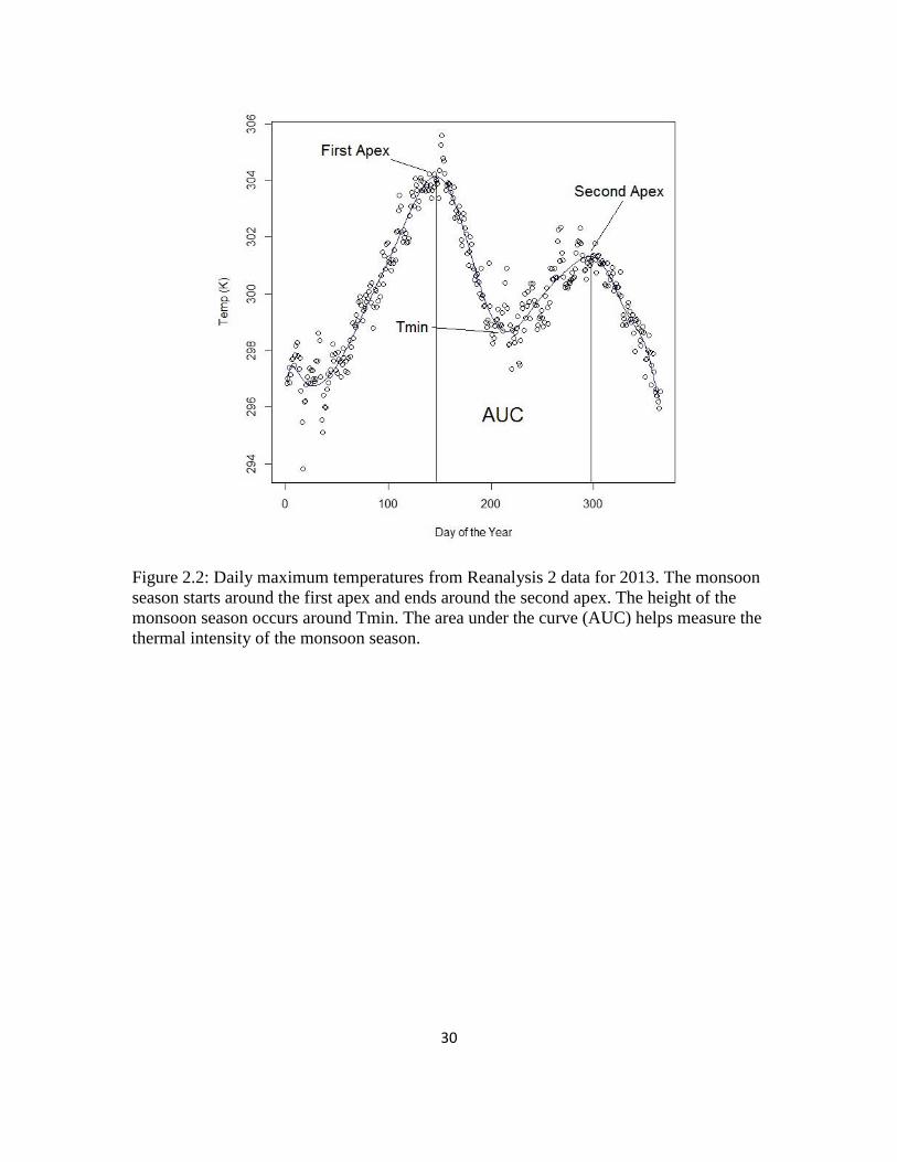
Figure 2.2 shows the maximum daily temperature progression for 2013 along with
a fitted curved derived from a 15th order polynomial regression. Two apices and a local
minimum distinctly occur during the late spring, summer, and fall season (Figure 2.2).
These three model parameters are part of a U-shaped curve that defines the progression of
the monsoon season. These model parameters are labeled: first apex (season start or
onset), Tmin (peak intensity or the bottom of the U-shaped curve), and second apex
(season end or withdrawal).
30
Figure 2.2: Daily maximum temperatures from Reanalysis 2 data for 2013. The monsoon
season starts around the first apex and ends around the second apex. The height of the
monsoon season occurs around Tmin. The area under the curve (AUC) helps measure the
thermal intensity of the monsoon season.
31
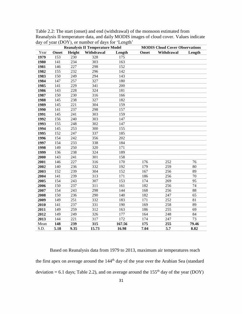
Table 2.2: The start (onset) and end (withdrawal) of the monsoon estimated from
Reanalysis II temperature data, and daily MODIS images of cloud cover. Values indicate
day of year (DOY), or number of days for ‘Length’ Reanalysis II Temperature Model MODIS Cloud Cover Observations
Year Onset Height Withdrawal Length Onset Withdrawal Length
1979 153 230 328 175
1980 141 234 303 163
1981 146 227 298 152
1982 155 232 296 142
1983 150 249 294 143
1984 147 257 327 180
1985 141 229 341 200
1986 143 228 324 181
1987 150 230 316 166
1988 145 238 327 182
1989 145 221 304 159
1990 141 237 298 157
1991 145 241 303 159
1992 156 240 303 147
1993 155 248 302 147
1994 145 253 300 155
1995 152 247 337 185
1996 154 242 356 202
1997 154 233 338 184
1998 149 250 320 171
1999 136 238 324 189
2000 143 241 301 158
2001 146 227 316 170 176 252 76
2002 140 236 332 192 179 259 80
2003 152 239 304 152 167 256 89
2004 141 239 313 171 186 256 70
2005 154 243 307 153 174 269 95
2006 150 237 311 161 182 256 74
2007 154 243 298 144 168 256 88
2008 150 236 290 140 182 247 65
2009 149 251 332 183 171 252 81
2010 141 237 331 190 169 258 89
2011 149 259 312 163 186 255 69
2012 149 249 326 177 164 248 84
2013 144 221 317 172 174 247 73
Mean 148 239 315 167.56 175 255 79.46
S.D. 5.18 9.35 15.73 16.98 7.04 5.7 8.82
Based on Reanalysis data from 1979 to 2013, maximum air temperatures reach
the first apex on average around the 144th day of the year over the Arabian Sea (standard
deviation = 6.1 days; Table 2.2), and on average around the 155th day of the year (DOY)
32
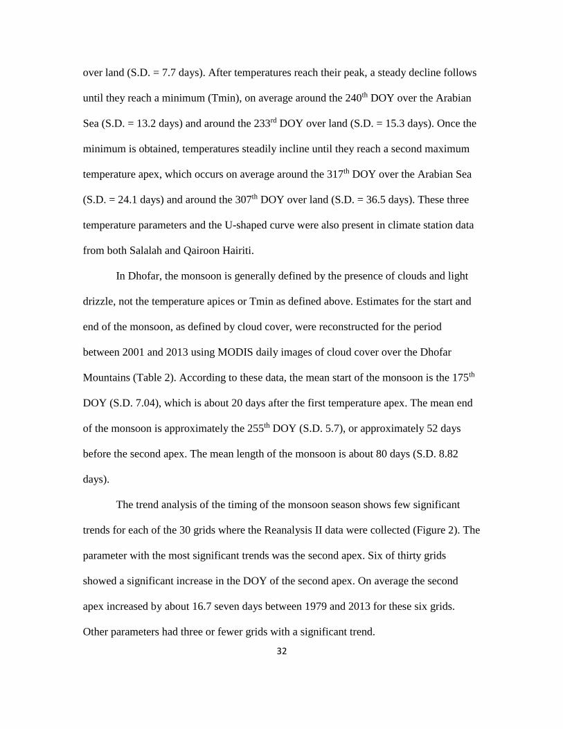
over land (S.D. = 7.7 days). After temperatures reach their peak, a steady decline follows
until they reach a minimum (Tmin), on average around the 240th DOY over the Arabian
Sea (S.D. = 13.2 days) and around the 233rd DOY over land (S.D. = 15.3 days). Once the
minimum is obtained, temperatures steadily incline until they reach a second maximum
temperature apex, which occurs on average around the 317th DOY over the Arabian Sea
(S.D. = 24.1 days) and around the 307th DOY over land (S.D. = 36.5 days). These three
temperature parameters and the U-shaped curve were also present in climate station data
from both Salalah and Qairoon Hairiti.
In Dhofar, the monsoon is generally defined by the presence of clouds and light
drizzle, not the temperature apices or Tmin as defined above. Estimates for the start and
end of the monsoon, as defined by cloud cover, were reconstructed for the period
between 2001 and 2013 using MODIS daily images of cloud cover over the Dhofar
Mountains (Table 2). According to these data, the mean start of the monsoon is the 175th
DOY (S.D. 7.04), which is about 20 days after the first temperature apex. The mean end
of the monsoon is approximately the 255th DOY (S.D. 5.7), or approximately 52 days
before the second apex. The mean length of the monsoon is about 80 days (S.D. 8.82
days).
The trend analysis of the timing of the monsoon season shows few significant
trends for each of the 30 grids where the Reanalysis II data were collected (Figure 2). The
parameter with the most significant trends was the second apex. Six of thirty grids
showed a significant increase in the DOY of the second apex. On average the second
apex increased by about 16.7 seven days between 1979 and 2013 for these six grids.
Other parameters had three or fewer grids with a significant trend.
33
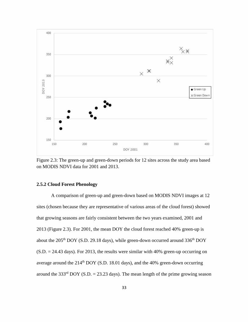
Figure 2.3: The green-up and green-down periods for 12 sites across the study area based
on MODIS NDVI data for 2001 and 2013.
2.5.2 Cloud Forest Phenology
A comparison of green-up and green-down based on MODIS NDVI images at 12
sites (chosen because they are representative of various areas of the cloud forest) showed
that growing seasons are fairly consistent between the two years examined, 2001 and
2013 (Figure 2.3). For 2001, the mean DOY the cloud forest reached 40% green-up is
about the 205th DOY (S.D. 29.18 days), while green-down occurred around 336th DOY
(S.D. = 24.43 days). For 2013, the results were similar with 40% green-up occurring on
average around the 214th DOY (S.D. 18.01 days), and the 40% green-down occurring
around the 333rd DOY (S.D. = 23.23 days). The mean length of the prime growing season
34
was about 130 days (S.D. = 9.71 days) in 2001, and 118 days (S.D. = 9.98 days) in 2013.
With regards to land cover, grass covers generally began their prime growing season
earlier than tree covers (mean = 199th DOY, S.D. 18.66 days) and ended earlier (mean =
323rd DOY, S.D. 17.88 days) than tree covers (green-up: mean = 217th DOY, S.D. 24.04
days; mean green-down = 344th DOY, S.D. 21.42 days). For shrub covers, the start and
end of prime growing was between the grass and forest covers (mean green-up = 206th
DOY, S.D. 26.25 days; the mean green-down = 327th DOY, S.D. 26.08 days).
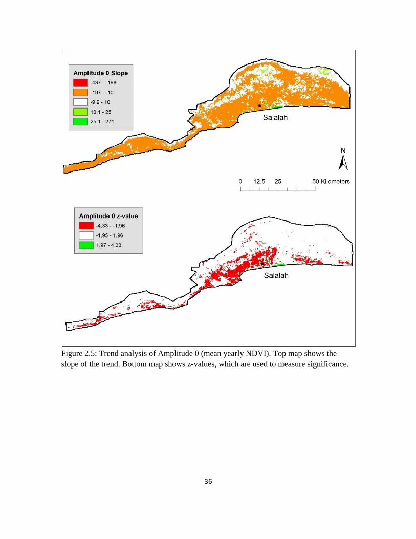
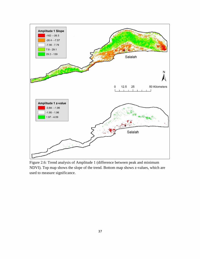
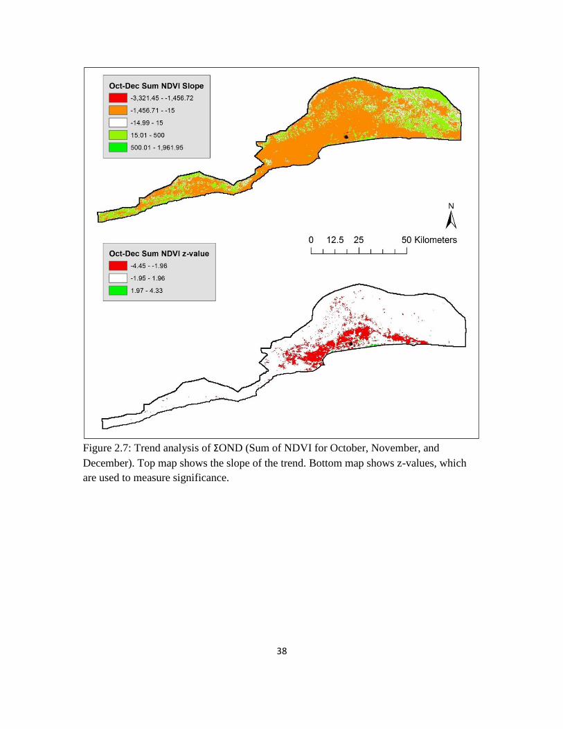
The results of the seasonal trend analyses are shown in Figures 2.4, 2.5, 2.6, and
2.7. Amplitude 0 and Amplitude 1 trends (Figures 2.5 and 2.6) are negative mainly
around the city of Salalah (see details in Galletti et al. forthcoming). The ΣOND (Figure
2.7) trends also show significant negative trends along the coast near the city of Salalah,
which may indicate declining vegetation due to human activity near the city. The timing
of the peak growing season (Phase 1; Figure 2.4) appears to be significant at only two
primary clusters: one around the western edge of the cloud forest, and another on the
eastern edge. Both of these clusters show significant negative trends, indicating that the
growing season starts earlier (approximately 3-4 days earlier in the west and 2-14 days
earlier in the east). The rest of the image, with the exception of small pockets here and
there, shows mainly no significant Phase 1 trends.
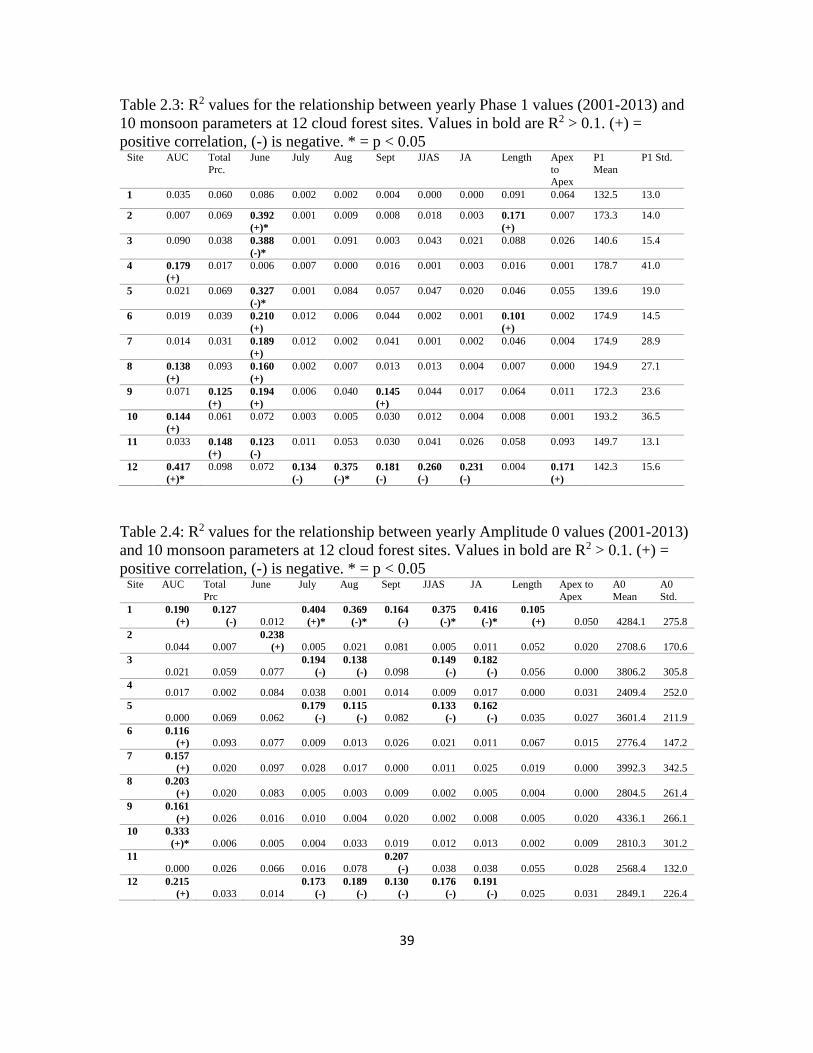
Correlations between the key seasonal parameters (Amplitude 0, Amplitude 1,
Phase 1, and ΣOND) and climate variables showed mainly weak to moderate correlation
and no systematic correlation across the 12 sites (Tables 2.3, 2.4, 2.5, and 2.6). Phase 1
revealed weak to moderate correlation with June precipitation, but there were
inconsistencies between negative and positive correlations. Amplitude 0 showed weak to

35
moderate positive correlation to AUC, while Amplitude 1 showed weak to moderate
negative correlation with June and July precipitation across several sites. ΣOND showed
mainly weak correlation to all climate variables.
Figure 2.4: Trend analysis of Phase 1 (timing of the peak of the cycle). Top map shows
the slope of the trend (change in NDVI/year). Bottom map shows z-values, which are
used to measure significance.
36
Figure 2.5: Trend analysis of Amplitude 0 (mean yearly NDVI). Top map shows the
slope of the trend. Bottom map shows z-values, which are used to measure significance.
37
Figure 2.6: Trend analysis of Amplitude 1 (difference between peak and minimum
NDVI). Top map shows the slope of the trend. Bottom map shows z-values, which are
used to measure significance.
38
Figure 2.7: Trend analysis of ΣOND (Sum of NDVI for October, November, and
December). Top map shows the slope of the trend. Bottom map shows z-values, which
are used to measure significance.
39
Table 2.3: R2 values for the relationship between yearly Phase 1 values (2001-2013) and
10 monsoon parameters at 12 cloud forest sites. Values in bold are R2 > 0.1. (+) =
positive correlation, (-) is negative. * = p < 0.05 Site AUC Total
Prc.
June July Aug Sept JJAS JA Length Apex
to Apex
P1
Mean
P1 Std.
1 0.035 0.060 0.086 0.002 0.002 0.004 0.000 0.000 0.091 0.064 132.5 13.0
2 0.007 0.069 0.392
(+)*
0.001 0.009 0.008 0.018 0.003 0.171
(+)
0.007 173.3 14.0
3 0.090 0.038 0.388
(-)*
0.001 0.091 0.003 0.043 0.021 0.088 0.026 140.6 15.4
4 0.179
(+)
0.017 0.006 0.007 0.000 0.016 0.001 0.003 0.016 0.001 178.7 41.0
5 0.021 0.069 0.327
(-)*
0.001 0.084 0.057 0.047 0.020 0.046 0.055 139.6 19.0
6 0.019 0.039 0.210
(+)
0.012 0.006 0.044 0.002 0.001 0.101
(+)
0.002 174.9 14.5
7 0.014 0.031 0.189
(+)
0.012 0.002 0.041 0.001 0.002 0.046 0.004 174.9 28.9
8 0.138
(+)
0.093 0.160
(+)
0.002 0.007 0.013 0.013 0.004 0.007 0.000 194.9 27.1
9 0.071 0.125
(+)
0.194
(+)
0.006 0.040 0.145
(+)
0.044 0.017 0.064 0.011 172.3 23.6
10 0.144
(+)
0.061 0.072 0.003 0.005 0.030 0.012 0.004 0.008 0.001 193.2 36.5
11 0.033 0.148
(+)
0.123
(-)
0.011 0.053 0.030 0.041 0.026 0.058 0.093 149.7 13.1
12 0.417
(+)*
0.098 0.072 0.134
(-)
0.375
(-)*
0.181
(-)
0.260
(-)
0.231
(-)
0.004 0.171
(+)
142.3 15.6
Table 2.4: R2 values for the relationship between yearly Amplitude 0 values (2001-2013)
and 10 monsoon parameters at 12 cloud forest sites. Values in bold are R2 > 0.1. (+) =
positive correlation, (-) is negative. * = p < 0.05 Site AUC Total
Prc
June July Aug Sept JJAS JA Length Apex to
Apex
A0
Mean
A0
Std.
1 0.190
(+)
0.127
(-) 0.012 0.404
(+)*
0.369
(-)*
0.164
(-)
0.375
(-)*
0.416
(-)*
0.105
(+) 0.050 4284.1 275.8
2
0.044 0.007 0.238
(+) 0.005 0.021 0.081 0.005 0.011 0.052 0.020 2708.6 170.6
3
0.021 0.059 0.077 0.194
(-)
0.138
(-) 0.098 0.149
(-)
0.182
(-) 0.056 0.000 3806.2 305.8
4 0.017 0.002 0.084 0.038 0.001 0.014 0.009 0.017 0.000 0.031 2409.4 252.0
5
0.000 0.069 0.062 0.179
(-)
0.115
(-) 0.082 0.133
(-)
0.162
(-) 0.035 0.027 3601.4 211.9
6 0.116
(+) 0.093 0.077 0.009 0.013 0.026 0.021 0.011 0.067 0.015 2776.4 147.2
7 0.157
(+) 0.020 0.097 0.028 0.017 0.000 0.011 0.025 0.019 0.000 3992.3 342.5
8 0.203
(+) 0.020 0.083 0.005 0.003 0.009 0.002 0.005 0.004 0.000 2804.5 261.4
9 0.161
(+) 0.026 0.016 0.010 0.004 0.020 0.002 0.008 0.005 0.020 4336.1 266.1
10 0.333
(+)* 0.006 0.005 0.004 0.033 0.019 0.012 0.013 0.002 0.009 2810.3 301.2
11
0.000 0.026 0.066 0.016 0.078 0.207
(-) 0.038 0.038 0.055 0.028 2568.4 132.0
12 0.215
(+) 0.033 0.014 0.173
(-)
0.189
(-)
0.130
(-)
0.176
(-)
0.191
(-) 0.025 0.031 2849.1 226.4
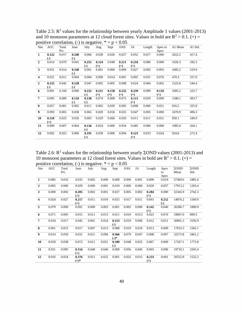
40
Table 2.5: R2 values for the relationship between yearly Amplitude 1 values (2001-2013)
and 10 monsoon parameters at 12 cloud forest sites. Values in bold are R2 > 0.1. (+) =
positive correlation, (-) is negative. * = p < 0.05 Site AUC Total
Prc.
June July Aug Sept JJAS JA Length Apex to
Apex
A1 Mean A1 Std.
1 0.122
(-)
0.017 0.240
(-)
0.066 0.028 0.020 0.027 0.052 0.017 0.000 2022.2 417.4
2 0.014 0.070 0.041 0.255
(-)
0.124
(+)
0.048 0.211
(+)
0.210
(+)
0.086 0.000 1026.3 182.5
3 0.031 0.014 0.140
(-)
0.061 0.001 0.006 0.009 0.027 0.002 0.003 1685.2 519.9
4 0.021 0.011 0.004 0.004 0.000 0.014 0.001 0.002 0.031 0.076 470.3 257.0
5 0.155
(-)
0.042 0.128
(-)
0.047 0.002 0.005 0.008 0.024 0.004 0.002 1525.8 544.4
6 0.001 0.104 0.000 0.232
(-)
0.211
(+)
0.158
(+)
0.232
(+)
0.239
(+)
0.099 0.116
(+)
1005.2 225.7
7 0.095 0.000 0.110
(-)
0.130
(-)
0.074 0.008 0.075 0.113
(+)
0.029 0.000 1580.1 493.7
8 0.057 0.001 0.002 0.011 0.003 0.020 0.005 0.008 0.000 0.021 916.5 325.9
9 0.093 0.005 0.038 0.065 0.020 0.016 0.025 0.047 0.005 0.000 1670.9 496.3
10 0.110
(+)
0.025 0.026 0.003 0.029 0.066 0.020 0.011 0.011 0.031 850.1 349.9
11 0.000 0.007 0.064 0.136
(-)
0.024 0.000 0.054 0.085 0.000 0.000 1085.0 204.1
12 0.002 0.023 0.006 0.191
(-)
0.039 0.000 0.094 0.123
(+)
0.033 0.024 924.6 272.4
Table 2.6: R2 values for the relationship between yearly ΣOND values (2001-2013) and
10 monsoon parameters at 12 cloud forest sites. Values in bold are R2 > 0.1. (+) =
positive correlation, (-) is negative. * = p < 0.05 Site AUC Total
Prc. June July Aug Sept JJAS JA Length Apex
to
Apex
ΣOND Mean
ΣOND Std.
1 0.085 0.010 0.035 0.002 0.000 0.000 0.000 0.001 0.000 0.019 37469.6 1881.6
2 0.002 0.000 0.029 0.000 0.001 0.019 0.000 0.000 0.020 0.057 17913.2 1203.4
3 0.000 0.002 0.205
(+)
0.002 0.001 0.027 0.005 0.002 0.284
(+)
0.000 32345.9 2762.3
4 0.024 0.027 0.217
(+)
0.011 0.010 0.025 0.017 0.011 0.001 0.252
(-)
14876.2 1569.9
5 0.079 0.009 0.091 0.000 0.003 0.001 0.002 0.000 0.142
(+)
0.040 30286.7 1889.9
6 0.071 0.005 0.015 0.011 0.013 0.011 0.010 0.013 0.023 0.076 18067.0 899.3
7 0.034 0.017 0.045 0.001 0.024 0.153
(-)
0.019 0.006 0.012 0.011 30001.3 3192.9
8 0.001 0.023 0.017 0.007 0.013 0.088 0.019 0.010 0.013 0.009 17033.3 1565.1
9 0.014 0.059 0.031 0.021 0.094 0.366
(-)*
0.079 0.047 0.008 0.007 32573.8 3461.2
10 0.018 0.038 0.072 0.011 0.051 0.189
(-)
0.048 0.025 0.067 0.000 17167.1 1773.8
11 0.021 0.095 0.154
(+)
0.040 0.046 0.000 0.056 0.045 0.003 0.096 19710.1 2265.4
12 0.016 0.054 0.376
(+)*
0.011 0.022 0.001 0.032 0.015 0.233
(+)
0.001 20552.8 1552.2
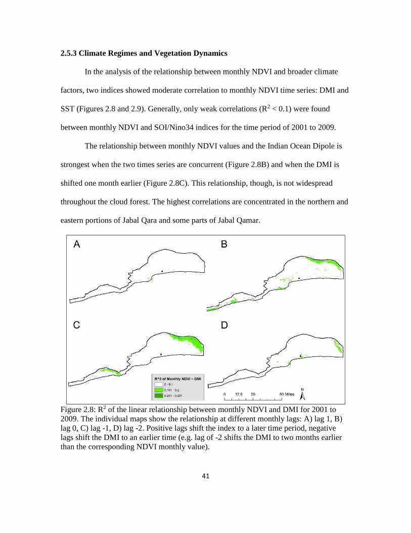
41
2.5.3 Climate Regimes and Vegetation Dynamics
In the analysis of the relationship between monthly NDVI and broader climate
factors, two indices showed moderate correlation to monthly NDVI time series: DMI and
SST (Figures 2.8 and 2.9). Generally, only weak correlations (R2 < 0.1) were found
between monthly NDVI and SOI/Nino34 indices for the time period of 2001 to 2009.
The relationship between monthly NDVI values and the Indian Ocean Dipole is
strongest when the two times series are concurrent (Figure 2.8B) and when the DMI is
shifted one month earlier (Figure 2.8C). This relationship, though, is not widespread
throughout the cloud forest. The highest correlations are concentrated in the northern and
eastern portions of Jabal Qara and some parts of Jabal Qamar.
Figure 2.8: R2 of the linear relationship between monthly NDVI and DMI for 2001 to
2009. The individual maps show the relationship at different monthly lags: A) lag 1, B)
lag 0, C) lag -1, D) lag -2. Positive lags shift the index to a later time period, negative
lags shift the DMI to an earlier time (e.g. lag of -2 shifts the DMI to two months earlier
than the corresponding NDVI monthly value).
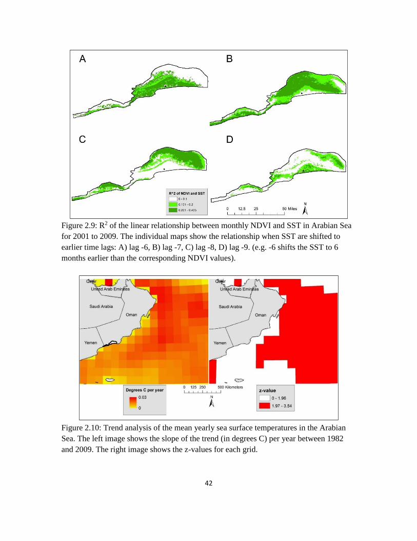
42
Figure 2.9: R2 of the linear relationship between monthly NDVI and SST in Arabian Sea
for 2001 to 2009. The individual maps show the relationship when SST are shifted to
earlier time lags: A) lag -6, B) lag -7, C) lag -8, D) lag -9. (e.g. -6 shifts the SST to 6
months earlier than the corresponding NDVI values).
Figure 2.10: Trend analysis of the mean yearly sea surface temperatures in the Arabian
Sea. The left image shows the slope of the trend (in degrees C) per year between 1982
and 2009. The right image shows the z-values for each grid.
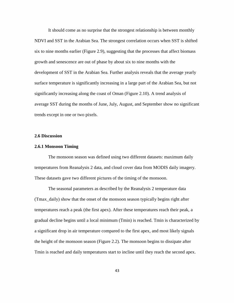
43
It should come as no surprise that the strongest relationship is between monthly
NDVI and SST in the Arabian Sea. The strongest correlation occurs when SST is shifted
six to nine months earlier (Figure 2.9), suggesting that the processes that affect biomass
growth and senescence are out of phase by about six to nine months with the
development of SST in the Arabian Sea. Further analysis reveals that the average yearly
surface temperature is significantly increasing in a large part of the Arabian Sea, but not
significantly increasing along the coast of Oman (Figure 2.10). A trend analysis of
average SST during the months of June, July, August, and September show no significant
trends except in one or two pixels.
2.6 Discussion
2.6.1 Monsoon Timing
The monsoon season was defined using two different datasets: maximum daily
temperatures from Reanalysis 2 data, and cloud cover data from MODIS daily imagery.
These datasets gave two different pictures of the timing of the monsoon.
The seasonal parameters as described by the Reanalysis 2 temperature data
(Tmax_daily) show that the onset of the monsoon season typically begins right after
temperatures reach a peak (the first apex). After these temperatures reach their peak, a
gradual decline begins until a local minimum (Tmin) is reached. Tmin is characterized by
a significant drop in air temperature compared to the first apex, and most likely signals
the height of the monsoon season (Figure 2.2). The monsoon begins to dissipate after
Tmin is reached and daily temperatures start to incline until they reach the second apex.
44
Once temperatures have reached this second apex, it is likely that the influence of
monsoon winds and colder SSTs off the coast of Arabia has completely subsided.
The onset and withdrawal of the monsoon is difficult to time precisely. Previous
studies have attempted to reconstruct the onset over the Indian Subcontinent (e.g. Fieux
and Stommel 1977; Joseph et al. 1994; Fasullo and Webster 2003; Joseph et al. 2006).
These studies have used a wide variety of indices to recreate the onset of the monsoon,
ranging from historical ship records (Fieux and Stommel 1977), to rain gauge data
(Joseph et al. 1994), to hydrological indices (Fasullo and Webster 2003). The biggest
discrepancy is that that neither of the two models developed in this study perfectly aligns
with the timing of the monsoon in these other studies. The mean onset of the monsoon
season, as modeled by the first apex in this paper, is very close to the dates of monsoon
onset reported in the other studies (e.g. Fieux and Stommel 1977; Joseph et al. 1994;
Fasullo and Webster 2003; Joseph et al. 2006).
Only one other study known to this author attempts to date the withdrawal of the
monsoon (Fasullo and Webster 2003), Based on the Hydrologic Onset and Withdrawal
index (HOWI) between 1948 and 2000, it concludes that the monsoon consistently ends
in August or September, and 48 of the 53 years reported in their study show the
withdrawal date between August 20th and September 27th. The model of monsoon timing
based on Reanalysis 2 results reported here indicates an end to the monsoon season
occurring much later in the year, but the model using the cloud cover data indicate
monsoon withdrawal around the same time as reported by Fasullo and Webster (2003),
between September 4th and September 26th for the period 2001 to 2013. The much later
dates reported by the second apex are likely a temperature progression influenced by
45
post-monsoon conditions. After the monsoon season, winds become weaker and shift to
an eastward source over the equator accompanied by warmer ocean water displacing
upwelling (Schott and McCreary 2001).
Addressing the monsoon season by temperature data from Reanalysis 2 provides a
set of conditions that are easily modeled using curve fitting; measuring the timing of the
monsoon becomes a simple task of extracting maxima, minima, and, if a general
measurement of intensity is desired, calculating the AUC for the season. For this reason,
it is a useful tool for understanding monsoon progression. But the model developed from
cloud cover data is more appropriate to measuring the actual onset and withdrawal of the
monsoon as it is experienced in southern Arabia (Hildebrandt and Eltahir 2007). This
model is assumed to be more accurate because it captures the conditions most associated
with the monsoon in southern Arabia: cloud fog driving an increase in ground moisture
(Hildebrandt 2005; Hildebrandt et al. 2006; Abdul-Wahab et al. 2007; Hildebrandt and
Eltahir 2007; Scholte and De Geest 2010). Indeed, most people living in Dhofar would
describe the start of the monsoon by consistent cloud cover and fog moisture, as well as a
general decrease in temperatures.
The limitation to using cloud cover data from sources like MODIS is that the
imagery can only capture a single snapshot at one point in time (during the morning).
While persistence of cloud cover is a defining characteristic of the monsoon in Dhofar,
there is a possibility that a morning snapshot could miss the formation of monsoon
clouds; during the visual analysis it was noted that some breaks in cloud cover, where
several images showed no cloud cover over the study area, occurred well into the
monsoon season. Another limitation is that cloud cover data alone does not predict
46
precipitation. The amount of fog moisture is critical for tree growth (Hildebrandt et al.
2007a,b). MODIS provides a two-dimensional snapshot of the Earth’s surface, but not
vertical measurements of cloud height or moisture content. Despite these limitations,
satellite imagery remains one of the best ways for determining the onset and withdrawal
of the monsoon season in southern Arabia.
The trend analyses show little evidence for widespread changes to the monsoon
timing. The model developed with Reanalysis 2 data had the longest time series and was
the primary focus for this analysis. The second apex showed some indication that it was
occurring later in the year, but only in a handful of the 30 grids. The trend of the timing
of the first apex and Tmin also gave little indication of significant change.
2.6.2 Phenology
The mean 40% green-up (start of the peak growing season) for 2001 and 2013
occurred about 30 to 40 days after the onset of the monsoon in Arabia, while the mean
40% green-down (senescence onset) occurred about 85 days after the monsoon ended.
Trees required about 2.5 more weeks than grasses to reach the 40% green-up mark, but
were able to stave off senescence for 3 weeks longer than grass covers. The rooting depth
is critical for water uptake in the cloud forest trees (Hildebrandt 2005), allowing them to
delay leaf fall until water stress reaches a critical juncture (Reich and Borchert 1984).
Horizontal precipitation is another factor in delaying tree senescence. Additional
moisture over tree canopy occurs because of turbulent redistribution and edge effects
(Hildebrandt 2005; Hildebrandt and Eltahir 2006; Hildebrandt and Eltahir 2007), and has
47
been shown to be critical in maintaining tree cover in Dhofar and promoting sapling
growth. Shrub phenology tended to be in the middle of these two covers.
2.6.3 Vegetation Dynamics and Climate Variability
The relationship between the seasonal vegetation parameters (Phase 1, Amplitude
0, Amplitude 1, and ΣOND) and climate variables showed some weak to moderate
correlation, but the lack of consistency suggests that the vegetation dynamics are mostly
resistant to the inter-annual variability of the ten climate variables used in this study
(Table 2.3, 2.4, 2.5, and 2.6). The timing of the peak NDVI (Phase 1) shows weak to
moderate correlation with June precipitation at 8 of the 12 sites (Table 2.3). This
correlation is likely related to the start of the monsoon. High amounts of precipitation in
June can signal an early start to the growing season. But, the positive and negative
correlation suggests that there is an inconsistency in the relationship between Phase 1 and
June precipitation. Amplitude 0 showed the most consistent correlations with AUC (6 of
12 sites with R2 > 0.1), and July and August precipitation. Amplitude 1 showed mainly
weak, but some moderate correlation with June, July, August, and September
precipitation. ΣOND showed little widespread correlation to any single variable.
These results suggest that precipitation and the AUC have some influence on
seasonal vegetation parameters, but they are not dominant in the cloud forest’s
phenology. There are two likely reasons for this. First, the cloud cover is a critical
climatic component in the success of the ecosystem’s ability to maintain high vegetation
density, despite the arid conditions of southern Arabia (Hildebrandt 2005; Hildebrandt et
al. 2007). Cloud cover reduces the effects of incoming shortwave solar radiation and
48
tempers evapotranspiration. Second, the moisture in the cloud fog is distributed through
horizontal precipitation (Hildebrandt 2005; Hildebrandt and Eltahir 2006; Hildebrandt
and Eltahir 2007) and wind speed (Abdul-Wahab 2007). Precipitation as measured by
climate stations may underestimate the amount of moisture transferred to the ground
during the monsoon because fog moisture redistributes through turbulence and edge
effects (Hildebrandt 2005; Hildebrandt and Eltahir 2007). Ideally, the relationship
between the seasonal vegetation parameters and climate should also include spatially and
temporally explicit fog moisture data. Despite the limitations in measuring precipitation,
the phenology of the cloud forest is remarkably resilient to the variability of measurable
precipitation, as well as the length of the monsoon and the AUC, apparently because of
the dichotomous and orographic nature of cloud cover during the monsoon season.
The trend analyses bolster the argument that the cloud forest is resilient in the face
of climate variability. The significant ΣOND, Amplitude 0, and Amplitude 1 trends are
primarily associated with the coastal plain, and likely linked to human impacts (Galletti et
al. forthcoming). The Phase 1 trends do show some changes in the seasonality of the
NDVI peak, mainly at two prominent clusters at the east and west margins that are
associated with a shift to earlier dates for Phase 1. A longer time series is required to
determine if this trend is indicative of climate changes or human impacts. Since these two
clusters sit on the margins, a climate explanation is possible if cloud cover, and thus
moisture potential, is changing over these areas. Another possible factor could be the
IOD. The relationship between NDVI time series and the DMI showed weak positive
correlations at the margins of the cloud forest (Figure 2.8). While these weak DMI
correlations are close in proximity, they did not overlap completely.
49
2.6.4 Vegetation Dynamics, Teleconnections, and Climate Regimes
Vegetation phenology has a week relationship with the DMI and a stronger
relationship with SST in the Arabian Sea. Correlations to ENSO were weak (R2 < 0.1),
which is perhaps not surprising since recent observations have shown a weakening in the
relationship between ENSO and ISM in the latter part of the 20th century (Kumar et al.
1999). The IOD is thought to directly influence monsoon conditions (Ashok et al. 2001;
Ashok et al. 2004). In addition, research shows that the ENSO might have connections
with the IOD (Allen et al. 2001), perhaps indicating that the ENSO indirectly affects
monsoon conditions, an issue of ongoing debate (Ihara et al. 2008). The strongest
correlation between the NDVI time series and DMI were at the margins of the cloud
forest, which suggests that most of the forest may be shielded from IOD events. The 13
years of NDVI observations used in this study may not be long enough to assess any low
frequency connections between the IOD and cloud forest vegetation. Previous research
on a connection between the IOD and rainfall in southern Arabia found no significant
relationship (Charabi 2009).
The connection between the SST in the Arabian Sea and vegetation dynamics in
the cloud forest shows the strongest correlation between any two variables tested in this
study. This correlation is positive and seems to be about six to nine months out of phase.
Thus, the SST acts as a leading indicator of NDVI values in the cloud forest. The strength
of this relationship is tied to the development of the monsoon. During the monsoon
season, SST becomes cooler because of upwelling by the Somali Current. The Somali
Current passes through the strait between the island of Socatra and the Horn of Africa in
late spring or early summer (Schott and McCreary 2001). The cooler SST and a shift in
50
wind direction (southwest) cause clouds to form when air masses over the ocean meet the
warmer air-flow over land.
The findings presented above suggest that the Dhofar cloud forest is resistant to
various climate variability, with the likely exception of shifts in SST. If this is the case,
then the biodiversity of the cloud forest may be protected from climate changes unless the
monsoon destabilizes over southern Arabia. Two hypothetical ways the monsoon can
destabilize are by 1) temperatures cooling over the Arabian land mass, and 2) the
upwelling off the Arabian coast being undermined by warming ocean temperatures.
Empirical observations and trend analyses of temperatures over the Arabian Peninsula
show significant warming (AlSarmi and Washington 2011), which eliminates cooling
land surface temperatures as a long-term threat. This leaves warming of SST off the coast
of Arabia as the likeliest threat to cloud forest flora. In the analysis from this paper, there
was no significant SST trend detected directly off the coast of southern Arabia; waters in
the central and eastern portions of the Arabian Sea are significantly warming though
(Figure 2.10). In the long term, changes to SST off the coast of Arabia require alterations
to upwelling, which would require heating of deeper ocean layers and the Somali
Current. Nieves and colleagues (2015) found that warming was occurring in the 100 to
300 meter layer of the Indian Ocean, but this seems to be isolated mainly to the eastern
Indian Ocean. If heating occurs to the subsurface waters of the Somali basin - where the
Somali Current forms - this could potentially change upwelling off the coast of Arabia
and thus impact cloud formation over Dhofar. As of now, a trend analysis (reported
earlier) on SST during the monsoon (June, July, August, and September) revealed no
51
significant warming trend for any of these months, but models should explore the
likelihood of this happening under future climate change scenarios.
2.7 Conclusion
The model of the monsoon season over the southern Arabian Peninsula based on
cloud cover data captures the onset and withdrawal more closely to that experienced by
those living in in the Dhofar area. While further confirmation is required, the model
appears to offer a promising way to determine empirically the timing of the monsoon.
The Dhofar cloud forest reaches its peak growing period about a month after the
monsoon’s onset and continues until several months after the monsoon’s withdrawal.
Weak to moderate correlations between certain monsoon variables and vegetation
seasonality parameters suggests that the cloud forest vegetation is resistant to fluctuations
in precipitation, monsoon length, and temperature. The precipitation connection is
masked by the source of water for the cloud forest, fog moisture, which is not measured
accurately in rain gauges. The cloud cover, which reduces evapotranspiration, is linked
closely to upwelling off the Arabian coast. Any warming to the Somali Current that
drives upwelling could alter monsoon conditions and cause changes to the cloud forest.
2.8 Acknowledgements
Support for this research was provided in part by a Fulbright grant to Oman
funded by the U.S. Department of State and sponsored by the Office of the Advisor to
His Majesty The Sultan for Economic Planning Affairs. Special thanks to Sanda Heinz,
Said Al-Saqri, Annette Patzelt, B. L. Turner II, Patricia Fall, and Soe Myint - all of whom
52
provided support and encouragement at various times during the research and writing of
this paper.
2.9 References
Abdul-Wahab, S. A., H. Al-Hinai, K. A. Al-Najar, and M. S. Al-Kalbani (2007), Fog
Water Harvesting: Quality of Fog Water Collected for Domestic and Agricultural
Use, Environ. Eng. Sci., 24(4), 446–456, doi:10.1089/ees.2006.06-0066.
Allan, R., D. Chambers, W. Drosdowsky, H. Hendon, M. Latif, N. Nicholls, I. Smith, R.
Stone, and Y. Tourre (2001), Is there an Indian Ocean dipole, and is it independent
of the El Niño - Southern Oscillation?, Clivar Exch., 6(3), 18–22.
AlSarmi, S., and R. Washington (2011), Recent observed climate change over the
Arabian Peninsula, J. Geophys. Res., 116(D11), D11109,
doi:10.1029/2010JD015459.
Anderson, D. M., J. T. Overpeck, and A. K. Gupta (2002), Increase in the Asian
southwest monsoon during the past four centuries., Science, 297(5581), 596–9,
doi:10.1126/science.1072881.
Ashok, K., Z. Guan, and T. Yamagata (2001), Impact of the Indian Ocean Dipole on the
Relationship between the Indian Monsoon Rainfall and ENSO, Geophys. Res. Lett.,
28(23), 4499–4502, doi:10.1029/2001GL013294.
Ashok, K., Z. Guan, N. H. Sagi, and T. Yagamata (2004), Individual and Combined
influences of ENSO and the\rIndian Ocean Dipole on the Indian Summer Monsoon,
J. Clim., 17(16), 3141–3155, doi:10.1175/1520-
0442(2004)017<3141:IACIOE>2.0.CO;2.
Blechschmidt, I., A. Matter, F. Preusser, and D. Rieke-Zapp (2009), Monsoon triggered
formation of Quaternary alluvial megafans in the interior of Oman, Geomorphology,
110(3-4), 128–139, doi:10.1016/j.geomorph.2009.04.002.
Charabi, Y. (2009), Arabian summer monsoon variability: Teleconexion to ENSO and
IOD, Atmos. Res., 91(1), 105–117, doi:10.1016/j.atmosres.2008.07.006.
Charabi, Y., and S. A. Abdul-Wahab (2009), Synoptic aspects of the summer monsoon of
southern Oman and its global teleconnections, J. Geophys. Res. Atmos., 114(7), 1–9,
doi:10.1029/2008JD010234.
53
Cremaschi, M., and F. Negrino (2005), Evidence for an abrupt climatic change at 8700
14C yr B.P. in rockshelters and caves of Gebel Qara (Dhofar-Oman):
Palaeoenvironmental implications, Geoarchaeology, 20(6), 559–579,
doi:10.1002/gea.20068.
Eastman, J. R., F. Sangermano, B. Ghimire, H. Zhu, H. Chen, N. Neeti, Y. Cai, E. a.
Machado, and S. C. Crema (2009), Seasonal trend analysis of image time series, Int.
J. Remote Sens., 30(10), 2721–2726, doi:10.1080/01431160902755338.
Eastman, J. R., F. Sangermano, E. a. Machado, J. Rogan, and A. Anyamba (2013),
Global trends in seasonality of Normalized Difference Vegetation Index (NDVI),
1982-2011, Remote Sens., 5(10), 4799–4818, doi:10.3390/rs5104799.
Fasullo, J., and P. J. Webster (2003), A hydrological definition of Indian Monsoon onset
and withdrawal, J. Clim., 16(19), 3200–3211, doi:10.1175/1520-
0442(2003)016<3200a:AHDOIM>2.0.CO;2.
Fieux, M., and H. Stommel (1977), Onset of the Southwest Monsoon over the Arabian
Sea from Marine Reports of Surface Winds: Structure and Variability, Mon.
Weather Rev., 105(2), 231–236.
Flagg, C. N., and H. S. Kim (1998), Upper ocean currents in the northern Arabian Sea
from shipboard ADCP measurements collected during the 1994-1996 U.S. JGOFS
and ONR programs, Deep. Res. Part II Top. Stud. Oceanogr., 45(10-11), 1917–
1959, doi:10.1016/S0967-0645(98)00059-9.
Fleitmann, D., and A. Matter (2009), The speleothem record of climate variability in
Southern Arabia, Comptes Rendus Geosci., 341(8-9), 633–642,
doi:10.1016/j.crte.2009.01.006.
Fleitmann, D., S. J. Burns, M. Mudelsee, U. Neff, J. Kramers, A. Mangini, and A. Matter
(2003), Holocene forcing of the Indian monsoon recorded in a stalagmite from
southern Oman, Science (80-. )., 300(5626), 1737–1739,
doi:10.1126/science.1083130.
Fleitmann, D., S. J. Burns, U. Neff, M. Mudelsee, A. Mangini, and A. Matter (2004),
Palaeoclimatic interpretation of high-resolution oxygen isotope profiles derived
from annually laminated speleothems from Southern Oman, Quat. Sci. Rev., 23(7-8),
935–945, doi:10.1016/j.quascirev.2003.06.019.
Fleitmann, D., S. J. Burns, M. Pekala, A. Mangini, A. Al-Subbary, M. Al-Aowah, J.
Kramers, and A. Matter (2011), Holocene and Pleistocene pluvial periods in Yemen,
southern Arabia, Quat. Sci. Rev., 30(7-8), 783–787,
doi:10.1016/j.quascirev.2011.01.004.
54
Ghazanfar, S. (1998), Status of the flora and plant conservation in the sultanate of Oman,
Biol. Conserv., 85(5), 1167–1179.
Ghazanfar, S. A., and M. Fisher (eds) (1998), Vegetation of the Arabian Peninsula, edited
by S. A. Ghazanfar and M. Fisher, Kluwer Academic Publishers, Dordrecht.
Gupta, A. K., D. M. Anderson, and J. T. Overpeck (2003), Abrupt changes in the Asian
southwest monsoon during the Holocene and their links to the North Atlantic Ocean,
Nature, 421(6921), 354–7, doi:10.1038/nature01340.
Hildebrandt, A. (2005), Ecohydrology of a Seasonal Cloud Forest in Dhofar, PhD.
Dissertation, Massachusetts Institute of Technology.
Hildebrandt, A., and E. A. B. Eltahir (2006), Forest on the edge: Seasonal cloud forest in
Oman creates its own ecological niche, Geophys. Res. Lett., 33(11), 2–5,
doi:10.1029/2006GL026022.
Hildebrandt, A., and E. a. B. Eltahir (2007), Ecohydrology of a seasonal cloud forest in
Dhofar: 2. Role of clouds, soil type, and rooting depth in tree-grass competition,
Water Resour. Res., 43(11), n/a–n/a, doi:10.1029/2006WR005262.
Hildebrandt, A., M. Al Aufi, M. Amerjeed, M. Shammas, and E. A. B. Eltahir (2007),
Ecohydrology of a seasonal cloud forest in Dhofar: 1. Field experiment, Water
Resour. Res., 43(10), 1–13, doi:10.1029/2006WR005261.
Ihara, C., Y. Kushnir, and M. a. Cane (2008), Warming trend of the Indian Ocean SST
and Indian Ocean dipole from 1880 to 2004, J. Clim., 21(10), 2035–2046,
doi:10.1175/2007JCLI1945.1.
IPCC (2014), Synthesis Report. Contribution of Working Groups I, II and III to the Fifth
Assessment Report of the Intergovernmental Panel on Climate Change, edited by C.
W. Team, R. K. Pachauri, and L. A. Meyer, IPCC, Geneva, Switzerland.
Janzen, J. (1986), Nomads in the sultanate of Oman: tradition and development in
Dhofar, Westview Press, Boulder.
Janzen, J. (2000), The destruction of resources among the mountain nomads of Dhofar, in
The Transformation of Nomadic Society in the Arab East, edited by M. Mundy and
B. Musallam, pp. 160–175, Cambridge University Press, Cambridge, UK.
Joseph, P. V., J. K. Eischeid, and R. J. Pyle (1994), Interannual Variability of the Onset
of the Indian Summer Monsoon and Its Association with Atmospheric Features, El
Niño, and Sea Surface Temperature Anomalies, J. Clim., 7(1), 81–105,
doi:10.1175/1520-0442(1994)007<0081:IVOTOO>2.0.CO;2.
55
Joseph, P. V., K. P. Sooraj, and C. K. Rajan (2006), The Summer Monsoon Onset
Process Over South Asia and an Objective Method for the Date of Monsoon Onset
over Kerala, Int. J. Climatol., 26, 1871–1893, doi:10.1002/joc.1340.
Justice, C. O. et al. (1998), The Moderate Resolution Imaging Spectroradiometer
(MODIS): land remote sensing for global change research, IEEE Trans. Geosci.
Remote Sens., 36(4), 1228–1249, doi:10.1109/36.701075.
Kanamitsu, M., W. Ebisuzaki, J. Woollen, S.-K. Yang, J. J. Hnilo, M. Fiorino, and G. L.
Potter (2002), NCEP–DOE AMIP-II Reanalysis (R-2), Bull. Am. Meteorol. Soc.,
83(11), 1631–1643, doi:10.1175/BAMS-83-11-1631.
Krishnan, R., T. P. Sabin, D. C. Ayantika, a. Kitoh, M. Sugi, H. Murakami, a. G. Turner,
J. M. Slingo, and K. Rajendran (2013), Will the South Asian monsoon overturning
circulation stabilize any further?, Clim. Dyn., 40(1-2), 187–211,
doi:10.1007/s00382-012-1317-0.
Krishnaswamy, J., S. Vaidyanathan, B. Rajagopalan, M. Bonell, M. Sankaran, R. S.
Bhalla, and S. Badiger (2014), Non-stationary and non-linear influence of ENSO
and Indian Ocean Dipole on the variability of Indian monsoon rainfall and extreme
rain events, Clim. Dyn., doi:10.1007/s00382-014-2288-0.
Kumar, K. K., B. Rajagopalan, and M. A. Cane (1999), On the Weakening Relationship
Between the Indian Monsoon and ENSO, Science, 284(5423), 2156–2159,
doi:10.1126/science.284.5423.2156.
Kumar, K. K., B. Rajagopalan, M. Hoerling, G. Bates, and M. Cane (2006), Unraveling
the mystery of Indian monsoon failure during El Niño, Science, 314(5796), 115–
119.
Kürschner, H., P. Hein, N. Kilian, and M. A. Hubaishan (2004), The Hybantho durae-
Anogeissetum dhofaricae ass. nova - phytosociology, structure and ecology of an
endemic South Arabian forest community, Phytocoenologia, 34, 569–612.
Kwarteng, A. Y., S. Dorvlo, and G. T. V. Kumar (2009), Analysis of a 27-year rainfall
data (1977 – 2003) in the Sultanate of Oman, Int. J. Climatol., 617(July 2008), 605–
617, doi:10.1002/joc.
Miller, A. G., and M. Morris (1988), Plants of Dhofar, the southern region of Oman,
traditional, economic and medicinal uses, Office of the Adviser for Conservation of
the Environment, Diwan of Royal Court, Sultanate of Oman.
Nieves, V., J. K. Willis, and W. C. Patzert (2015), Recent hiatus caused by decadal shift
in Indo-Pacific heating, Science, 349(6247), 532–535.
56
Overpeck, J. T., D. Anderson, S. Trumbore, and W. Prell (1996), The southwest Indian
Monsoon over the last 18,000 years, Clim. Dyn., 12, 213–225.
Parker, A. G., and J. I. Rose (2008), Climate change and human origins in southern
Arabia, Proc. Semin. Arab. Stud., 38, 25–42.
Patzelt, A. (2011), The Themeda Quadrivalvis Tall-Grass Savannah of Oman At the
Crossroad Between Africa and Asia, Edinburgh J. Bot., 68(02), 301–319,
doi:10.1017/S0960428611000217.
Pickering, H. A., and A. Patzelt (2008), Field Guide to the Wild Plants of Oman, Kew
Publishing, Richmond, UK.
Rayner, N. A., D. E. Parker, E. B. Horton, C. K. Folland, L. V. Alexander, D. P. Rowell,
E. C. Kent, and A. Kaplan (2003), Global analyses of sea surface temperature, sea
ice, and night marine air temperature since the late Nineteenth Century, J. Geophys.
Res., 108, doi:10.1029/2002JD002670.
Reich, P. B., and R. Borchert (1984), Water Stress and Tree Phenology in a Tropical Dry
Forest in the Lowlands of Costa Rica, J. Ecol., 72(1), 61–74.
Reynolds, R. W., N. a. Rayner, T. M. Smith, D. C. Stokes, and W. Wang (2002), An
improved in situ and satellite SST analysis for climate, J. Clim., 15(13), 1609–1625,
doi:10.1175/1520-0442(2002)015<1609:AIISAS>2.0.CO;2.
Saji, N. H., B. N. Goswami, P. N. Vinayachandran, and T. Yamagata (1999), A dipole
mode in the tropical Indian Ocean, Nature, 401, 360–363.
Scholte, P., and P. De Geest (2010), The climate of Socotra Island (Yemen): A first-time
assessment of the timing of the monsoon wind reversal and its influence on
precipitation and vegetation patterns, J. Arid Environ., 74(11), 1507–1515,
doi:10.1016/j.jaridenv.2010.05.017.
Schott, F. A., and J. P. McCreary (2001), The monsoon circulation of the Indian Ocean,
Prog. Oceanogr., 51(1), 1–123, doi:10.1016/S0079-6611(01)00083-0.
Sen, P. K. (1968), Estimates of the regression coefficient based on Kendall’s tau, J. Am.
Stat. Assoc., 63, 1379–1389.
Shi, W., J. M. Morrison, E. Böhm, and V. Manghnani (2000), The Oman upwelling zone
during 1993, 1994 and 1995, Deep. Res. Part II Top. Stud. Oceanogr., 47(7-8),
1227–1247, doi:10.1016/S0967-0645(99)00142-3.
Theil, H. (1950), A rank-invariant method of linear and polynomial regression analysis, I,
II, III, Proc. K. Ned. Acad. van Wet., 53(386), 386–392, 512–525, 1397–1412.

57
Trenberth, K. E. (1984), Signal Versus Noise in the Southern Oscillation, Mon. Weather
Rev., 112(2), 326–332, doi:10.1175/1520-0493(1984)112<0326:SVNITS>2.0.CO;2.
58
CHAPTER 3
DRIVERS OF PLANT DIVERSITY IN THE SOUTH ARABIAN CLOUD FOREST1
“No amount of book learning will make a man a scientific man: nothing but patient
observation, and quiet and fair thought over what he has observed. He must go out for
himself, see for himself, compare and judge for himself, in the field, the quarry, the
cutting. He must study rocks, ores, fossils, in the nearest museum; and thus store in his
head, not with words, but with facts. He must verify – as far as he can – what he reads in
books, by his own observation; and be slow to believe anything, even on the highest
scientific authority, till he has either seen it, or something like enough to it to make it
seem to him probable, or at least possible.” (Charles Kingsley, 1873, x)
3.1 Abstract
The South Arabian Cloud Forest is a drought deciduous semi-arid forest on the
southern coast of the Arabian Peninsula. We describe the vegetation diversity of the
South Arabian Cloud Forest and test three hypotheses to explain biodiversity patterns of
woody plant species: (H1) neutral processes, (H2) biological interactions, and (H3)
environmental gradients. We collected plant density, cover, and frequency at 102 sample
points and estimated relative species abundances across two biomes: grasslands and
forests. Cluster analysis, Mantel correlograms, and canonical correspondence analysis
(CCA) are used to test our hypotheses.
The cluster analysis identified five vegetation groups. The two largest groups are
dominated by a small number of species. Anogeissus dhofarica and Commiphora spp.
account for 49% of the relative species abundance in forest plots, while Calotropis
procera, Commiphora spp., and Solanum incanum account for 42% of the relative
abundance in grassland plots. Based on our analyses, the (H2) biological interaction
1 Co-authored with Patricia L. Fall
59
hypothesis offers the best explanation for biodiversity patterns in the cloud forest.
However, the reason for this differs between the forest and grasslands. In forests, the
diversity patterns are dominated by a few species of trees and shrubs (A. dhofarica and
Commiphora spp.), most likely as a result of the region’s biogeographical history. In
grassland areas, however, diversity patterns are best explained as products of human
activity. Conservation efforts should focus on rarer species, which drive diversity
gradients across the region and are at risk of endangerment.
3.2 Introduction
The South Arabian Cloud Forest extends from the arid, southern reaches of
Yemen east to the Dhofar Mountains of southern Oman. Plant surveys and
biogeographical studies reveal a rich flora (Radcliffe Smith 1980; Miller and Morris
1988; Pickering and Patzelt 2008; Patzelt 2011) thought to be a remnant of a xerotropical
forest with paleo-African origins that stretched from Africa to Asia during the Tertiary
(Kürschner et al. 2004). Expanding populations and encroaching human influences
threaten the biodiversity of the cloud forest, making it critical to understand the
ecological structure of this unique ecosystem (Schlect et al. 2014).

60
Table 3.1: Three hypotheses and three tests of the drivers of plant diversity in the South
Arabian Cloud Forest. Under each test, the expected outcome and variables used in the
test are listed.
Test
Hypothesis Cluster
Analysis
Canonical
Correspondence
Analysis
Mantel Correlogram
H1: Neutral
processes
No clear pattern
of dominance in
species
abundances by a
few species
Variable: number
of dominant
species per
cluster group
CCA explains less than 30%
of the variance in the species
abundances
Variable: species abundance
as measured by importance
value (IV). Environmental
variables include climatic
and physiographic
Significant spatial
autocorrelation shown with
distance decay in the
correlation
Variable: beta diversity
measured using Brey-Curtis
and based on species
abundances using
importance value (IV)
H2: Biological
interactions
Few species with
high abundances
Variable: number
of dominant
species per
cluster group
CCA explains less than 30%
of the variance in the species
abundances
Variable: species abundance
as measured by importance
value (IV). Environmental
variables include climatic
and physiographic
No spatial autocorrelation,
or varying positive and
negative spatial correlation
Variable: beta diversity
measured using Brey-Curtis
and based on species
abundances using
importance value (IV))
H3:
Environmental
gradients
No clear pattern
of dominance in
species
abundances by a
few species
Variable: number
of dominant
species per
cluster group
CCA explains more than
30% of the variance in the
species abundances
Variable: species abundance
as measured by importance
value (IV). Environmental
variables include climatic
and physiographic
Significant spatial
autocorrelation shown with
distance decay in the
correlation
Variable: beta diversity
measured using Brey-Curtis
and based on species
abundances using
importance value (IV)
The cloud forest is a drought deciduous forest (Hildebrandt and Eltahir 2006;
Hildebrandt and Eltahir 2007; Hildebrandt et al. 2007), supported by ample summer rain
and cloud cover that compensate for limited precipitation through the rest of the year.
While most of the Arabian Peninsula has low vegetation density indicative of arid
regions, grasslands and forests flourish along the south facing slopes of the southern
mountains of Yemen and Oman, giving the cloud forest a semi-arid, and sometimes
61
tropical, demeanor. During the summer months, temperature differentials between the
Arabian Peninsula and the Arabian Sea cause clouds to form along the south-facing
slopes of the mountains. The temperature differential between the land and sea cause the
formation of the Indian Ocean Monsoon (also known locally as khareef), which provides
the precipitation and cloud cover that allow flora to thrive in an otherwise arid region.
Much of the vegetation senesces by December, where weather patterns return to the more
dryland conditions that dominate most of Arabia. Beyond the coastal mountains, the
characteristic desert ecosystem of the Arabian Peninsula prevails, and some floral species
that thrive deep in the desert can be found in parts of the cloud forest.
Despite the uniqueness of the cloud forest, few studies assess its floral
distribution, and understanding of its biodiversity remains limited. Understanding the
drivers of biodiversity of the cloud forest will be crucial for its conservation. Neutral
processes, defined by the limited dispersal capabilities of many species, help explain
patterns of biodiversity in a wide range of biogeographical studies (e.g., Rosindell et al.
2011). Alternatively, biodiversity patterns may be dominated by the wide distribution of
a few key taxa (e.g., Condit et al. 2002), particularly certain endemic species (Anogeissus
dhofarica and Maytenus dhofarensis), as well as plant species common across South
Arabia (Calotropis procera, Commiphora spp. and Ficus spp.). Finally, environmental
filtering could lead to certain species populating specific niche environments (Shmida
and Wilson 1985; Dauby et al. 2014). The cloud forest ecosystem features two distinct
vegetation types (forests and grasslands) and a high level of topographic variability over
short distances that separate forested regions from grasslands. We test three hypotheses to
explain the biodiversity of the South Arabian Cloud Forest (Table 3.1).
62
Neutral Processes (H1). The neutral processes hypothesis explains biodiversity as
the outcome of random processes and the limited dispersal capabilities of species
(Hubbell 2006; Chisolm and Pacala 2010; Rosindell et al. 2011). According to this
hypothesis, plant species are competitively equivalent, and through time biotic and
stochastic processes can lead to certain taxa becoming more prevalent than others,
resulting in spatially autocorrelated beta diversity patterns. Neutral processes would
result in plant survey sites being more similar when they are closer spatially and
progressively become less similar with distance; but no clear environmental gradient
would explain diversity patterns.
Biological Interactions (H2). Studies of tropical forests, particularly in the
Amazon, reveal that tree species diversity patterns are characterized by a small number of
dominant species and low beta diversity (Pitman et al. 1999, 2001; Legendre et al. 2005;
Tuomisto and Ruokolainen 2006). Biological interactions hypotheses (as part of dispersal
theory) are thus used to explain patterns of community structure based on relatively
homogeneous taxonomic composition and the wide distribution of a few dominant
species. The spatial structure of beta diversity has no clear spatial autocorrelation, nor
does it suggest that environmental factors explain patterns of diversity.
Environmental Gradients (H3). Niche environments that favor certain species can
explain variation in species diversity. Diversity patterns that are influenced by
environmental factors lead to various species flourishing in niches and, thus, diversity
patterns between similar environmental contexts would match more closely than those
that are in different environmental contexts. An analysis of the spatial patterning would
reveal similarity amongst closely situated sites, and a strong correlation between

63
environmental factors and diversity patterns would exist. This hypothesis would predict
spatial autocorrelation in beta diversity, and environmental variables would largely
account for the variance in species abundances.
Conservation approaches related to (H1) neutral processes and (H2) biological
interactions could be more regional in scope (e.g. Mac Nally 2007), where landscape-
wide decisions about conservation would need to be made. Alternatively, conservation
related to (H3) environmental gradients may entail a sampling of niches or targeting of
certain environmental conditions (Rickbeil et al. 2014).
3.3 Study Area
The South Arabian Cloud Forest is wedged between the Arabian Sea and the
desert gravel plains of the Nejd Plateau. Mountains run along the southern reaches of the
Dhofar region in Oman to Al Mahra in Yemen. Research has shown that Arabia was
more pluvial in the deep past, particularly during the last interglacial and the early
Holocene (e.g., Fleitmann and Matter 2009). Today, the climate is dry most of the year
except during the summer months when monsoon clouds blanket the region in mist
(Kwarteng et al. 2007; AlSarmi and Washington 2011). During the monsoon,
temperatures cool and precipitation increases dramatically, which allows vegetation in
the cloud forest to flourish, and supports broadleaf trees, which are rare on the Arabian
Peninsula.
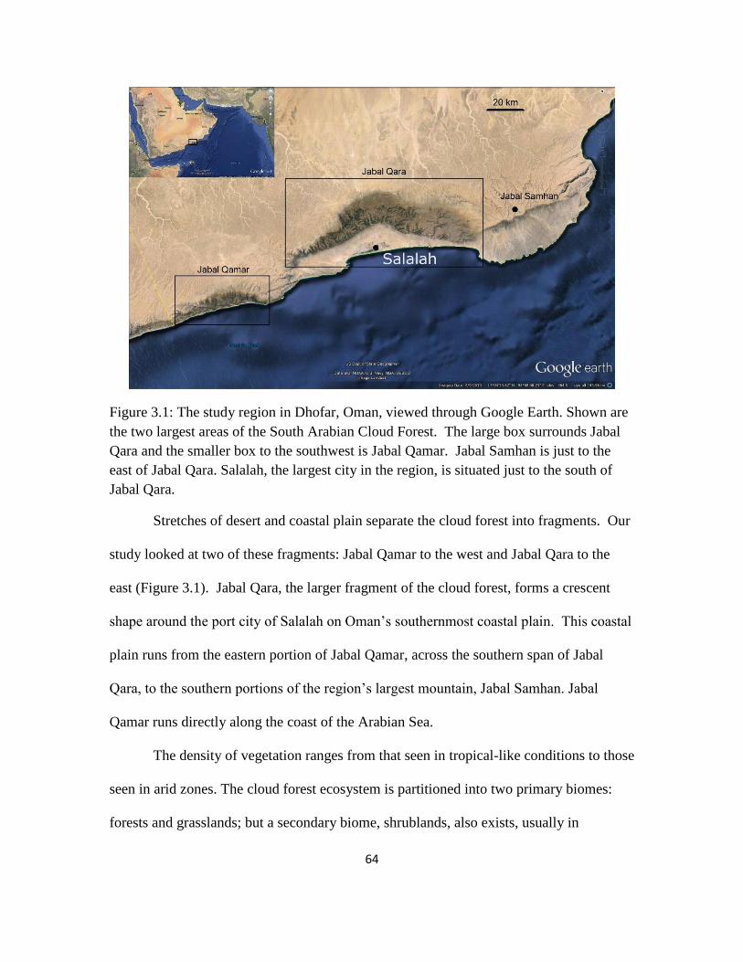
64
Figure 3.1: The study region in Dhofar, Oman, viewed through Google Earth. Shown are
the two largest areas of the South Arabian Cloud Forest. The large box surrounds Jabal
Qara and the smaller box to the southwest is Jabal Qamar. Jabal Samhan is just to the
east of Jabal Qara. Salalah, the largest city in the region, is situated just to the south of
Jabal Qara.
Stretches of desert and coastal plain separate the cloud forest into fragments. Our
study looked at two of these fragments: Jabal Qamar to the west and Jabal Qara to the
east (Figure 3.1). Jabal Qara, the larger fragment of the cloud forest, forms a crescent
shape around the port city of Salalah on Oman’s southernmost coastal plain. This coastal
plain runs from the eastern portion of Jabal Qamar, across the southern span of Jabal
Qara, to the southern portions of the region’s largest mountain, Jabal Samhan. Jabal
Qamar runs directly along the coast of the Arabian Sea.
The density of vegetation ranges from that seen in tropical-like conditions to those
seen in arid zones. The cloud forest ecosystem is partitioned into two primary biomes:
forests and grasslands; but a secondary biome, shrublands, also exists, usually in
65
association with the parts of the cloud forest that are more arid. Foothills leading up to
the mountains of Dhofar are vegetated with a mixture of forests, shrublands and
grasslands, usually with decreasing plant density as one approaches the sea. The
vegetation in the cloud forest is associated with the Saharo-Sindian and Saharo-Arabian
phytogeographic zones (Ghazanfar and Fisher 1998; Parker and Rose 2008), and it is
thought that the forests are a remnant of a much bigger ancient forest that once stretched
from Africa to India and possibly beyond (Kürschner et al. 2004).
3.4 Materials and Methods
3.4.1 Fieldwork and Floral Survey
Data on tree and shrub distributions were collected during fieldwork conducted
between January and April 2013. Random points were generated using ArcGIS across
the cloud forest, and each of these points was used to identify a survey sample point (89
random points). The study area was isolated for selection of these random points using a
mask of high NDVI pixels (>.1 in an October 2000 Landsat 7 image) plus a 1000 m
buffer. Thirteen additional non-random points were selected to provide coverage of areas
or terrains that were underrepresented in the distribution of the random points, making a
total of 102 sample points. Data on trees and shrubs were measured using the point-
centered quarter method (PCQM; Mitchell 2007). Absolute plant density (no./m2), cover
(basal area/hectare), and frequency (%/sample point) were measured for all woody
species along a westerly transect from each sample point.
For each sample point we determined the mean distance r, which is the sum of the
distances to the measured trees divided by the number of quarters (j) at a subsample point

66
(i). Subsample points are points at each of our sample points where observations were
made. For each sample point, we used about five subsample points, and each subsample
point is divided into four quarters. 𝑅𝑖𝑗 is the total distance between the species and our
random sample points in meters, 𝑛𝑖 is the number of subsample sample points (following
Mitchell 2007):
�̅� = ∑ ∑ 𝑅𝑖𝑗
𝑛𝑗=1
𝑛𝑖=1
4𝑛𝑖
Absolute density may be estimated as:
𝑑 = 1
�̅�2
Absolute cover is first calculated by estimating the planar area of each species’ trunk.
𝐴 =𝑐2
4𝜋
in which c is the circumference of the species trunk, and A (the planar area) is divided by
the number of species (𝑛𝑠) per sample point to arrive at the mean basal area (MBA):
𝑀𝐵𝐴 =𝐴
𝑛𝑠
The absolute coverage of a species (measured as total basal area per hectare) at a sample
point is calculated as:
𝑐 = 𝑀𝐵𝐴 ∗ 𝑑 ∗ 1 𝑚2
10,000 𝑐𝑚2
Finally, absolute species frequency is calculated as:
𝑓 =𝑛𝑢𝑚𝑏𝑒𝑟 𝑜𝑓 𝑠𝑢𝑏𝑠𝑎𝑚𝑝𝑙𝑒 𝑝𝑜𝑖𝑛𝑡𝑠 𝑤ℎ𝑒𝑟𝑒 𝑎 𝑠𝑝𝑒𝑐𝑖𝑒𝑠 𝑖𝑠 𝑜𝑏𝑠𝑒𝑟𝑣𝑒𝑑
𝑡𝑜𝑡𝑎𝑙 𝑛𝑢𝑚𝑏𝑒𝑟 𝑜𝑓 𝑠𝑢𝑏𝑠𝑎𝑚𝑝𝑙𝑒 𝑝𝑜𝑖𝑛𝑡𝑠∗ 100
f is measured as a percentage.
67
Relative density, cover, and frequency were calculated by dividing each of these
three metrics by the sum total of each metric for all species per sample point. We also
calculated importance values (IV) (relative cover + relative density + relative frequency =
IV) (sensu Mitchell 2007), which estimate the relative abundance of each species per
sample point. Our cluster analysis, Mantel correlograms, and canonical correspondence
analysis (CCA) use importance values as measures of species abundances.
3.4.2 Environmental and Climate Data
Temperature and precipitation data were obtained from the Bioclim dataset
(Hijmans et al. 2005). Rasters were used to represent precipitation and temperature
variables (see Appendix A, Table A.1). Physiographic variables (elevation, slope, aspect,
and hydrology) were derived from the SRTM 90m digital elevation model. The
hydrology raster shows the distance of any pixel to the nearest “stream” pixel, which
estimates proximity to locations where precipitation aggregates, such as wadis. Aspect is
split into two different raster variables: northness (cosine of aspect) and eastness (sine of
the aspect). In total, the analyses used 18 variables (see Appendix A).
3.4.3 Cluster Analysis
Cluster analysis was used to group the 102 sample points according to species
similarity and dissimilarity based on relative species importance values. A Bray-Curtis
index was used to measure ecological differences between sample points. The resulting
dendrograms are generated using Ward linkage. A classification tree indicates how
clusters are separated according to environmental variables. Misclassification rates and a
68
confusion matrix were used to assess the classification tree. Once the clusters were
identified, we summed the importance values for each species across the cluster groups.
Silhouette widths were used to evaluate how well the cluster groups were partitioned
based on the composition of species in each group (Rousseeuw 1987), and are interpreted
similarly to a correlation coefficient (see Appendix B).
3.4.4 Mantel Correlogram
Mantel correlograms were used to measure the spatial autocorrelation of beta
diversity of species between sample points (Borcard and Legendre 2012). Beta diversity
was measured using distance matrices. Importance values (IV) measure species
abundance at each site. Dissimilarity between sites was measured using the Bray-Curtis
index. Before the correlogram was computed, the dissimilarity matrix was spatially
detrended. The significance of groups in the correlograms was computed based on 999
permutations of the data. We used progressive correction and p-value adjustments for
multiple testing, as suggested by Legendre and Legendre (2012) and Borcard et al.
(2011).
3.4.5 Canonical Correspondence Analysis
We used canonical correspondence analysis (CCA; ter Braak 1986) to analyze
relationships between species abundances (as measured using IV) and environmental
gradients, based on 20 environmental variables (see discussion above) and a stepwise
variable selection function. An F test was used to determine a parsimonious number of
explanatory variables. Once this subset of variables was isolated using the method
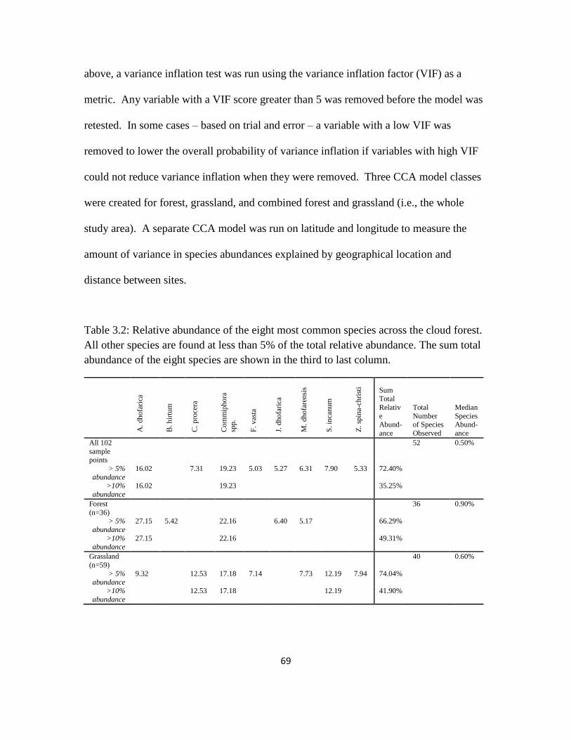
69
above, a variance inflation test was run using the variance inflation factor (VIF) as a
metric. Any variable with a VIF score greater than 5 was removed before the model was
retested. In some cases – based on trial and error – a variable with a low VIF was
removed to lower the overall probability of variance inflation if variables with high VIF
could not reduce variance inflation when they were removed. Three CCA model classes
were created for forest, grassland, and combined forest and grassland (i.e., the whole
study area). A separate CCA model was run on latitude and longitude to measure the
amount of variance in species abundances explained by geographical location and
distance between sites.
Table 3.2: Relative abundance of the eight most common species across the cloud forest.
All other species are found at less than 5% of the total relative abundance. The sum total
abundance of the eight species are shown in the third to last column.
A.
dho
fari
ca
B. h
irtu
m
C. p
roce
ra
Co
mm
ipho
ra
spp.
F.
vas
ta
J. d
ho
fari
ca
M. dh
ofa
rensi
s
S.
inca
nu
m
Z.
spin
a-ch
rist
i
Sum Total
Relativ
e Abund-
ance
Total
Number of Species
Observed
Median
Species Abund-
ance
All 102
sample points
52 0.50%
> 5%
abundance
16.02 7.31 19.23 5.03 5.27 6.31 7.90 5.33 72.40%
>10%
abundance
16.02 19.23 35.25%
Forest
(n=36)
36 0.90%
> 5%
abundance
27.15 5.42 22.16 6.40 5.17 66.29%
>10%
abundance
27.15 22.16 49.31%
Grassland
(n=59)
40 0.60%
> 5% abundance
9.32 12.53 17.18 7.14 7.73 12.19 7.94 74.04%
>10%
abundance
12.53 17.18 12.19 41.90%
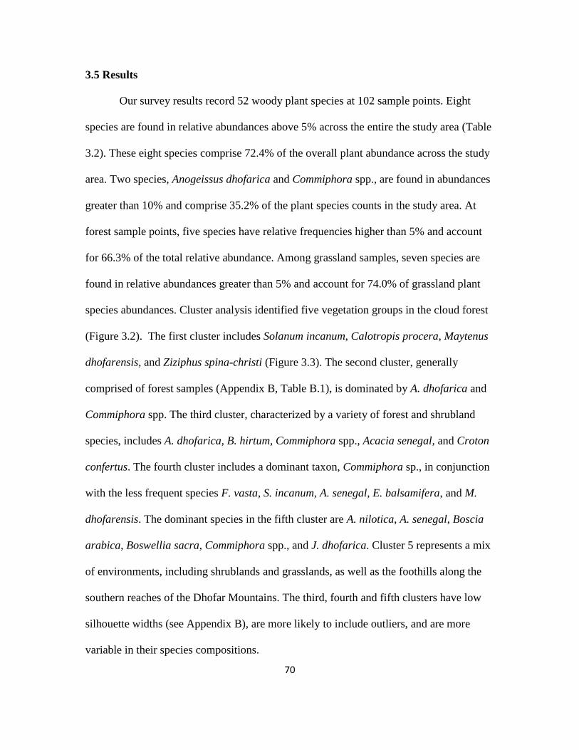
70
3.5 Results
Our survey results record 52 woody plant species at 102 sample points. Eight
species are found in relative abundances above 5% across the entire the study area (Table
3.2). These eight species comprise 72.4% of the overall plant abundance across the study
area. Two species, Anogeissus dhofarica and Commiphora spp., are found in abundances
greater than 10% and comprise 35.2% of the plant species counts in the study area. At
forest sample points, five species have relative frequencies higher than 5% and account
for 66.3% of the total relative abundance. Among grassland samples, seven species are
found in relative abundances greater than 5% and account for 74.0% of grassland plant
species abundances. Cluster analysis identified five vegetation groups in the cloud forest
(Figure 3.2). The first cluster includes Solanum incanum, Calotropis procera, Maytenus
dhofarensis, and Ziziphus spina-christi (Figure 3.3). The second cluster, generally
comprised of forest samples (Appendix B, Table B.1), is dominated by A. dhofarica and
Commiphora spp. The third cluster, characterized by a variety of forest and shrubland
species, includes A. dhofarica, B. hirtum, Commiphora spp., Acacia senegal, and Croton
confertus. The fourth cluster includes a dominant taxon, Commiphora sp., in conjunction
with the less frequent species F. vasta, S. incanum, A. senegal, E. balsamifera, and M.
dhofarensis. The dominant species in the fifth cluster are A. nilotica, A. senegal, Boscia
arabica, Boswellia sacra, Commiphora spp., and J. dhofarica. Cluster 5 represents a mix
of environments, including shrublands and grasslands, as well as the foothills along the
southern reaches of the Dhofar Mountains. The third, fourth and fifth clusters have low
silhouette widths (see Appendix B), are more likely to include outliers, and are more
variable in their species compositions.
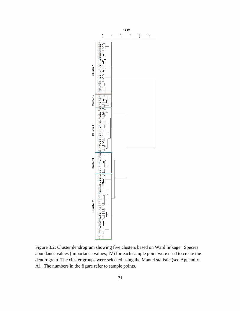
71
Figure 3.2: Cluster dendrogram showing five clusters based on Ward linkage. Species
abundance values (importance values; IV) for each sample point were used to create the
dendrogram. The cluster groups were selected using the Mantel statistic (see Appendix
A). The numbers in the figure refer to sample points.
72
Figure 3.3: Species abundances in each of the five cluster groups based on importance
values (IV).
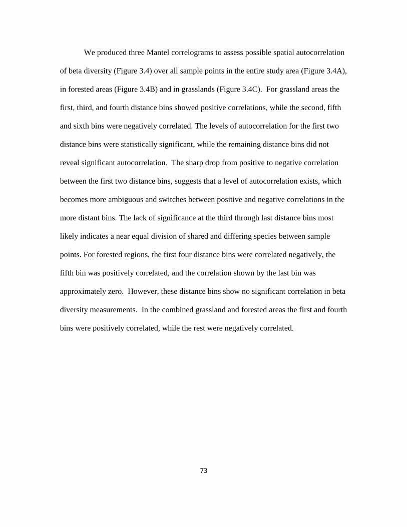
73
We produced three Mantel correlograms to assess possible spatial autocorrelation
of beta diversity (Figure 3.4) over all sample points in the entire study area (Figure 3.4A),
in forested areas (Figure 3.4B) and in grasslands (Figure 3.4C). For grassland areas the
first, third, and fourth distance bins showed positive correlations, while the second, fifth
and sixth bins were negatively correlated. The levels of autocorrelation for the first two
distance bins were statistically significant, while the remaining distance bins did not
reveal significant autocorrelation. The sharp drop from positive to negative correlation
between the first two distance bins, suggests that a level of autocorrelation exists, which
becomes more ambiguous and switches between positive and negative correlations in the
more distant bins. The lack of significance at the third through last distance bins most
likely indicates a near equal division of shared and differing species between sample
points. For forested regions, the first four distance bins were correlated negatively, the
fifth bin was positively correlated, and the correlation shown by the last bin was
approximately zero. However, these distance bins show no significant correlation in beta
diversity measurements. In the combined grassland and forested areas the first and fourth
bins were positively correlated, while the rest were negatively correlated.
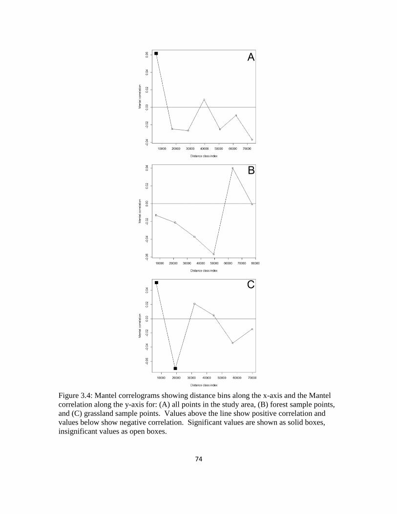
74
Figure 3.4: Mantel correlograms showing distance bins along the x-axis and the Mantel
correlation along the y-axis for: (A) all points in the study area, (B) forest sample points,
and (C) grassland sample points. Values above the line show positive correlation and
values below show negative correlation. Significant values are shown as solid boxes,
insignificant values as open boxes.
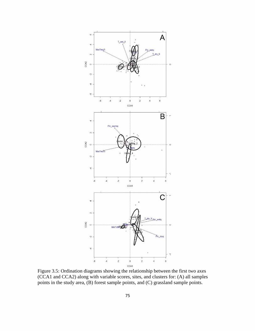
75
Figure 3.5: Ordination diagrams showing the relationship between the first two axes
(CCA1 and CCA2) along with variable scores, sites, and clusters for: (A) all samples
points in the study area, (B) forest sample points, and (C) grassland sample points.
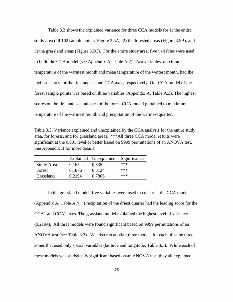
76
Table 3.3 shows the explained variance for three CCA models for 1) the entire
study area (all 102 sample points; Figure 3.5A), 2) the forested areas (Figure 3.5B), and
3) the grassland areas (Figure 3.5C). For the entire study area, five variables were used
to build the CCA model (see Appendix A, Table A.2). Two variables, maximum
temperature of the warmest month and mean temperature of the wettest month, had the
highest scores for the first and second CCA axes, respectively. Our CCA model of the
forest sample points was based on three variables (Appendix A, Table A.3). The highest
scores on the first and second axes of the forest CCA model pertained to maximum
temperature of the warmest month and precipitation of the warmest quarter.
Table 3.3: Variance explained and unexplained by the CCA analysis for the entire study
area, for forests, and for grassland areas. ***All three CCA model results were
significant at the 0.001 level or better based on 9999 permutations of an ANOVA test.
See Appendix B for more details.
Explained Unexplained Significance
Study Area 0.165 0.835 ***
Forest 0.1876 0.8124 ***
Grassland 0.2194 0.7806 ***
In the grassland model, five variables were used to construct the CCA model
(Appendix A, Table A.4). Precipitation of the driest quarter had the leading score for the
CCA1 and CCA2 axes. The grassland model explained the highest level of variance
(0.2194). All three models were found significant based on 9999 permutations of an
ANOVA test (see Table 3.3). We also ran another three models for each of same three
zones that used only spatial variables (latitude and longitude; Table 3.3). While each of
these models was statistically significant based on an ANOVA test, they all explained
77
low levels of variance (the highest = 0.1078 for forest sample plots), suggesting that
latitude and longitude tend to be weaker than environmental variables in explaining
species abundance in the cloud forest.
3.6 Discussion and Conclusions
Our results reveal that the diversity and distribution of woody plants differ
between the biomes of the cloud forest. If we consider the entire study area (all 102
sample points), the biological interactions hypothesis (H2) is affirmed most strongly,
based on three major results. First, eight species account for over 70% of the relative
species abundances, and just two species (A. dhofarica and Commiphora sp.) comprise
over 35% of the relative species abundances - while the median among all species is less
than 1%. The near ubiquitous distribution of A. dhofarica and Commiphora spp. defines
the phytosociological structure of the cloud forest (Kürschner et al. 2004), which also
lends support to our acceptance of this hypothesis. Second, our results show a lack of
spatial autocorrelation structure in our beta diversity measurements. While the first
distance bin (see Fig. 4A) shows significant correlation, the subsequent bins show mostly
negative (but not significant) spatial correlation. Both the lack of significance and only a
single positive correlation value at the fourth bin indicates that there is no clear spatial
correlation in the beta diversity over the entire study area. Third, the CCA model explains
less than 17% of the variance across the entire study area according to our environmental
variables. We would expect a higher level of explained variance if environmental
gradients (H3) best explained our patterns of biodiversity. But one other factor to
consider for why environmental gradients are not as strong of an explanation is that cloud
78
cover is the single most important environmental factor, to such an extent that its mere
presence is the one factor needed to sustain the environment (see Chapter 2). The clouds
are present at the start of the monsoon and persist throughout the monsoon season. There
seems to be little spatial variability. Thus the benefits of the cloud cover (reduced
evapotranspiration and fog moisture) are ubiquitous.
For forest sample plots, the biological interactions hypothesis (H2) again provides
the best explanation of diversity patterns. Only two taxa, A. dhofarica and Commiphora
spp., comprise the most prevalent species in forested areas, as seen in the cluster analysis
and relative taxonomic abundances. Cluster 2 is defined strongly by A. dhofarica and
Commiphora spp., and to a lesser extent by J. dhofarica. While Cluster 3 includes more
species, only five stand out: A. dhofarica, B. hirtum, Commiphora sp., A. Senegal, and C.
confertus. The success of A. dhofarica and Commiphora spp., both in terms of the cluster
analysis and their common occurrence at both forest and overall sample points, is perhaps
the strongest evidence that the biodiversity patterns in the cloud forest are rooted in the
dispersal success of these two species. The lack of spatial autocorrelation structure and
the low explained variance of the CCA analysis (less than 19%) are used to refute the
environmental gradients hypothesis (H3) and the neutral processes hypothesis (H1). The
biological interaction hypothesis (H2), which was developed from observations of
tropical forests (Pitman et al. 1999, 2001; Condit et al. 2002), similarly explains
biodiversity patterns best in the South Arabian Cloud Forest, which lies just outside of
the tropical zone. The cloud forest is derived from an ancient tropical forest (Kürschner et
al. 2004) and, accordingly, the species that populate the cloud forest today have evolved
from these tropical sources. As a contributing factor in this evolution, interglacials
79
between the Tertiary and present have included periods of much greater precipitation
(Burns et al. 2001; Fleitmann et al. 2004; Fleitmann and Matter 2009). This increased
precipitation may have expanded the cloud forest in conditions closer to those found in
modern tropical forests. Today, despite dry conditions during most of the year, the
modern monsoon season provides enough moisture for tropical conditions, and near
constant cloud cover, for a substantial part of the year.
In grassland areas, the biological interactions hypothesis (H2) also explains
diversity patterns most effectively, but most likely due to land-use decisions. Grazing
indicators (e.g., S. incanum and C. procera), as well as trees and shrubs found typically in
rangelands (e.g., Ficus sp., Z. spina-christi, and M. dhofarensis), prevail in Cluster 1
(Appendix A), to an extent that strongly supports the biological interactions hypothesis
(H2). The environmental gradients hypothesis is not supported in light of the low level of
overall explained variance (less than 22%), despite showing stronger explained variance
than in forested areas or the study area as a whole. The Mantel correlograms show
stronger evidence for spatial autocorrelation structure than in forested areas. The lack of
clear distance decay in Mantel correlograms and significance in the farthest distance bins
refute the neutral processes hypothesis (H1). The biological interactions hypothesis (H2)
explains diversity patterns in the grasslands based, in part, on the influences of human
activity, especially animal husbandry. Herds of camel, cattle, and goats are common
throughout the cloud forest. Among the plant species common to the grassland areas, S.
incanum and C. procera are poisonous to livestock (Miller and Morris 1988; Mekonnen
1994), giving these species a competitive advantage over other taxa that are more
80
palatable to livestock. Grassland areas also are flatter and more suitable for grazing large
herds.
Because the forested areas are dominated by a limited number of species with
wide dispersal capabilities, preservation of the cloud forest’s biodiversity will depend on
widespread adoption of conservation measures that protect rare species. Conservation has
been a priority in Dhofar for some time (Ghazanfar 1998) and its success will depend on
a comprehensive approach that focuses more on tree and shrub species that occur in
relatively low abundances. Regional conservation practices (i.e. conservation practices
aimed at the entire cloud forest, and not just certain parts) have been deemed important in
other cloud forests (Williams-Linera 2002) based on the heterogeneity of species
composition across short distances. A similar strategy might be needed in Dhofar, but for
different reasons. Pastoralism is a longstanding component of traditional society in
Dhofar (Janzen 1986), and vegetation across the region is increasingly impacted by
encroaching herds of camels, cattle and goats, as well as infrastructure development.
Restoration of biodiversity in grasslands is notoriously difficult without abandonment of
the range, or long-term relief from grazing activities (e.g. Vuorio et al. 2014), and recent
studies have shown that grasslands are often neglected in conservation efforts (Grau et al.
2014). Foothills areas, which are in close proximity to the city of Salalah, are vulnerable
to rapidly increasing urban expansion and other human activity. Forested areas are still
populated by a diverse array of floral species, but will require large intact protected
forests to reliably safeguard biodiversity (Berhane et al. 2015). Any conservation effort
will need to account for the variety of human activity, and, because the biodiversity
patterns are defined by the dominance of a small subset of species, priority should be

81
given to those species found in low abundance, mainly because they will have a greater
likelihood of becoming endangered. Conservation efforts in the grassland and shrubland
areas will most likely prove even more difficult without a significant restoration effort
that incorporates the range of socio-economic activities that are dependent on these
environments.
3.7 Acknowledgements
Much of the research was supported by work conducted through a Fulbright Grant
to Oman (awarded to Galletti) from the U.S. State Department and sponsored by The
Office of the Advisor to His Majesty The Sultan for Economic Planning Affairs. We
offer special thanks to Said Al-Saqri and Annette Patzelt for support during the Fulbright
grant period. Finally, we would like to thank Steven Falconer and Sanda Heinz for
assistance with data collection.
3.8 References
AlSarmi, S., and R. Washington (2011), Recent observed climate change over the
Arabian Peninsula, J. Geophys. Res., 116(D11), D11109,
doi:10.1029/2010JD015459.
Berhane, A., Ø. Totland, M. Haile, and S. R. Moe (2015), Intense use of woody plants in
a semiarid environment of Northern Ethiopia: Effects on species composition,
richness and diversity, J. Arid Environ., 114, 14–21,
doi:10.1016/j.jaridenv.2014.11.001.
Borcard, D., and P. Legendre (2012), Is the Mantel correlogram powerful enough to be
useful in ecological analysis? A simulation study, Ecology, 93(6), 1473–1481,
doi:10.1890/11-1737.1.
82
Borcard, D., F. Gillet, and P. Legendre (2011), Numerical Ecology with R, Springer, New
York.
Burns, S. J., D. Fleitmann, A. Matter, U. Neff, and A. Mangini (2001), Speleothem
evidence from Oman for continental pluvial events during interglacial periods,
Geology, 29(7), 623, doi:10.1130/0091-7613(2001)029<0623:SEFOFC>2.0.CO;2.
Chisholm, R. A., and S. W. Pacala (2010), Niche and neutral models predict
asymptotically equivalent species abundance distributions in high-diversity
ecological communities., Proc. Natl. Acad. Sci. U. S. A., 107(36), 15821–5,
doi:10.1073/pnas.1009387107.
Condit, R. et al. (2002), Beta-diversity in tropical forest trees, Science, 295(5555), 666–9,
doi:10.1126/science.1066854.
Dauby, G., O. J. Hardy, M. Leal, F. Breteler, and T. Stévart (2014), Drivers of tree
diversity in tropical rain forests: new insights from a comparison between littoral
and hilly landscapes of Central Africa, edited by P. Linder, J. Biogeogr., 41(3), 574–
586, doi:10.1111/jbi.12233.
Fleitmann, D., and A. Matter (2009), The speleothem record of climate variability in
Southern Arabia, Comptes Rendus Geosci., 341(8-9), 633–642,
doi:10.1016/j.crte.2009.01.006.
Fleitmann, D., S. J. Burns, U. Neff, M. Mudelsee, A. Mangini, and A. Matter (2004),
Palaeoclimatic interpretation of high-resolution oxygen isotope profiles derived
from annually laminated speleothems from Southern Oman, Quat. Sci. Rev., 23(7-8),
935–945, doi:10.1016/j.quascirev.2003.06.019.
Ghazanfar, S. (1998), Status of the flora and plant conservation in the sultanate of Oman,
Biol. Conserv., 85(3), 287–295, doi:10.1016/S0006-3207(97)00162-6.
Ghazanfar, S. A., and M. Fisher (eds) (1998), Vegetation of the Arabian Peninsula, edited
by S. A. Ghazanfar and M. Fisher, Kluwer Academic Publishers, Dordrecht.
Grau, H. R., R. Torres, N. I. Gasparri, P. G. Blendinger, S. Marinaro, and L. Macchi
(2014), Natural grasslands in the Chaco. A neglected ecosystem under threat by
agriculture expansion and forest-oriented conservation policies, J. Arid Environ., (in
press), doi:10.1016/j.jaridenv.2014.12.006.
Hijmans, R. J., S. E. Cameron, J. L. Parra, P. G. Jones, and A. Jarvis (2005), Very high
resolution interpolated climate surfaces for global land areas, Int. J. Climatol.,
25(15), 1965–1978, doi:10.1002/joc.1276.
83
Hildebrandt, A., and E. A. B. Eltahir (2006), Forest on the edge: Seasonal cloud forest in
Oman creates its own ecological niche, Geophys. Res. Lett., 33(11), 2–5,
doi:10.1029/2006GL026022.
Hildebrandt, A., and E. A. B. Eltahir (2007), Ecohydrology of a seasonal cloud forest in
Dhofar: 2. Role of clouds, soil type, and rooting depth in tree-grass competition,
Water Resour. Res., 43(11), 1–13, doi:10.1029/2006WR005262.
Hildebrandt, A., M. Al Aufi, M. Amerjeed, M. Shammas, and E. A. B. Eltahir (2007),
Ecohydrology of a seasonal cloud forest in Dhofar: 1. Field experiment, Water
Resour. Res., 43(10), 1–13, doi:10.1029/2006WR005261.
Hubbell, S. P. (2006), Neutral theory and the evolution of ecological equivalence,
Ecology, 87(6), 1387–1398.
Janzen, J. (1986), Nomads in the sultanate of Oman: tradition and development in
Dhofar, Westview Press, Boulder.
Kürschner, H., P. Hein, N. Kilian, and M. A. Hubaishan (2004), The Hybantho durae-
Anogeissetum dhofaricae ass. nova - phytosociology, structure and ecology of an
endemic South Arabian forest community, Phytocoenologia, 34, 569–612.
Kwarteng, A. Y., S. Dorvlo, and G. T. V. Kumar (2009), Analysis of a 27-year rainfall
data (1977 – 2003) in the Sultanate of Oman, Int. J. Climatol., 617(July 2008), 605–
617, doi:10.1002/joc.
Legendre, P., and L. Legendre (1998), Numerical ecology, Developments in evironmental
modelling, edited by S. E. Edition, Elsevier.
Legendre, P., D. Borcard, and P. R. Peres-Neto (2005), Analyzing beta diversity:
Partitioning the spatial variation of community composition data, Ecol. Monogr.,
75(4), 435–450.
Mekonnen, Y. (1994), A survey of plants (potentially) toxic to livestock in the Ethiopian
flora, Sinet, an Ethiop. J. Sci., 17(1), 9–32.
Miller, A. G., and M. Morris (1988), Plants of Dhofar, The Southern Region of Oman:
Traditional, Economic, and Medicinal Uses, Office of the Adviser for Conservation
of the Environment, Diwan of Royal Court, Sultanate of Oman.
Mitchell, K. (2007), Quantitative analysis by the point-centered quarter method, Geneva,
NY.
84
Mac Nally, R. (2007), Use of the abundance spectrum and relative-abundance
distributions to analyze assemblage change in massively altered landscapes, Am.
Nat., 170(3), 319–30, doi:10.1086/519859.
Parker, A. G., and J. I. Rose (2008), Climate change and human origins in southern
Arabia, Proc. Semin. Arab. Stud., 38, 25–42.
Patzelt, A. (2011), The Themeda Quadrivalvis Tall-Grass Savannah of Oman At the
Crossroad Between Africa and Asia, Edinburgh J. Bot., 68(02), 301–319,
doi:10.1017/S0960428611000217.
Pickering, H., and A. Patzelt (2008), Field Guide to the Wild Plants of Oman, Royal
Botanical Gardens, Kew, Kew, United Kingdom.
Pitman, N. C. A., J. Terborgh, M. R. Silman, and P. Nunez V. (1999), Tree Species
Distributions in an Upper Amazonian Forest, Ecology, 80(8), 2651–2661.
Pitman, N. C. A., J. W. Terborgh, M. R. Silman, P. N. V, A. David, C. E. Cerón, W. A.
Palacios, and M. Aulestia (2001), Dominance and Distribution of Tree Species in
Upper Amazonian Terra Firme Forests, Ecology, 82(8), 2101–2117.
Radcliffe Smith A (1980), The vegetation of Dhofar, in The scientific results of the Oman
Flora and Fauna Survey, 1977, (Dhofar), edited by N. Shaw-Reade, S, B. Sale, J, D.
Gallagher, M, and H. Daly, R, pp. 59–86.
Rickbeil, G. J. M., N. C. Coops, M. E. Andrew, D. K. Bolton, N. Mahony, and T. A.
Nelson (2014), Assessing conservation regionalization schemes: employing a beta
diversity metric to test the environmental surrogacy approach, edited by S. Ferrier,
Divers. Distrib., 20(5), 503–514, doi:10.1111/ddi.12146.
Rosindell, J., S. P. Hubbell, and R. S. Etienne (2011), The unified neutral theory of
biodiversity and biogeography at age ten., Trends Ecol. Evol., 26(7), 340–8,
doi:10.1016/j.tree.2011.03.024.
Rousseeuw, P. J. (1987), Silhouettes: A graphical aid to the interpretation and validation
of cluster analysis, J. Comput. Appl. Math., 20, 53–65, doi:10.1016/0377-
0427(87)90125-7.
Schlecht, E., L. G. H. Zaballos, D. Quiroz, P. Scholte, and A. Buerkert (2014),
Traditional land use and reconsideration of environmental zoning in the Hawf
Protected Area, south-eastern Yemen, J. Arid Environ., 109, 92–102,
doi:10.1016/j.jaridenv.2014.05.016.
Shmida, A., and M. V. Wilson (1985), Biological determinants of species diversity, J.
Biogeogr., 12(1), 1–20.

85
Tuomisto, H., and K. Ruokolainen (2006), Analyzing or explaining beta diversity?
Understanding the targets of different methods of analysis, Ecology, 87(11), 2697–
2708.
Vuorio, V., A. Muchiru, R. S. Reid, and J. O. Ogutu (2014), How pastoralism changes
savanna vegetation : impact of old pastoral settlements on plant diversity and
abundance in south-western Kenya, Biodivers. Conserv., 23, 3219–3240,
doi:10.1007/s10531-014-0777-4.
Williams-Linera, G. (2002), Tree species richness complementarity , disturbance and
fragmentation in a Mexican tropical montane cloud forest, Biodivers. Conserv., 11,
1825–1943.
86
CHAPTER 4
LAND CHANGES AND THEIR DRIVERS IN THE CLOUD FOREST AND
COASTAL ZONE OF DHOFAR, OMAN, BETWEEN 1988 AND 20132
4.1 Abstract
Several analyses are used to measure environmental changes in the cloud forest
and coastal plain in Dhofar, southern Oman, including a land change analysis, multiple
endmember spectral mixture analysis (MESMA), cluster analysis using local indicators
of spatial association (LISA), and trend analysis of NDVI time series. The results
demonstrate systematic degradation and loss of vegetation types in the cloud forest, and
loss of native land covers to impervious surfaces on the coastal plain; decreases in woody
plant vegetation in almost half of the cloud forest in distinctive hotspots of loss; and
significant decreases in NDVI trends around the city of Salalah, along the coastal plain,
and in parts of the cloud forest.
The proximate drivers of these changes in the cloud forest appear to be changes in
grazing activities, while the growth of Salalah, especially its peri-urban area, altered the
coastal plain. These drivers, in turn, are linked to distal ones, foremost changes in Omani
policies and investments in the Dhofar area, traced to government responses to the
Dhofar War (1970-1975), which have resulted in increased livestock populations and
urban growth.
2 Co-authored with B.L. Turner II and Soe W. Myint

87
4.2 Introduction
Deforestation and land degradation are recognized problems in dryland
environments that cover about 41% of the terrestrial surface of the Earth (Reynolds et al.
2007). Worldwide net primary production of grass- and rangelands has declined due to
intensified land uses (e.g., Bai et al. 2008; Li et al. 2012), and the loss of ecosystem
services to dryland degradation affects some 250 million people (Reynolds et al. 2007).
As a result, dryland deforestation and land degradation have drawn international attention
through such programs as the U.N.’s 1992 Convention to Combat Desertification (UNEP
1994) and the 2006 International Year of the Desert and Desertification.
The causes of this degradation, both climatic and anthropogenic in kind, have
drawn substantial research attention. Anthropogenic causes have been arrayed along a
continuum between proximate and distal causes, depending on the immediacy of human
activities and processes to the actual land change and consequences in question (Serneels
& Lambin 2001; Geist and Lambin 2002; Lambin et al. 2003; Turner et al. 2007).
Proximate causes, such as agricultural expansion or land-use intensification, are relatively
easy to correlate strongly with land changes, whereas distal causes (aka underlying or
root causes and teleconnections), such as international policies and markets, prove to be a
challenge, commonly linked to actual land changes conceptually or through
interpretations of case studies (Brannstrom & Vadjunec 2014; Lambin et al. 2001; Liu et
al. 2013; Vayda & Walters 1999). It is also recognized that distal and proximate causes
interact in ways that amplify or attenuate land change (Defries et al. 2010; Seto &
Reenberg 2014).

88
Dryland degradation, linked variously to proximate and distal causes, is apparent
in the southern Arabian Peninsula, including within the South Arabian Cloud Forest, near
Salalah, Dhofar, Oman. Cloud forest ecosystems generally occupy only a small portion of
the world’s forests, but are usually rich in ecosystem services and biodiversity (Higuera
et al. 2013). Dhofar’s portion of the South Arabian Cloud Forest consists of forest, shrub,
and grasslands that have been decreasing in biomass and tree species during the lifetime
of satellite observations of the region. The causes of this change—climatic, owing to
changes in the Indian Ocean monsoon (Kumar et al. 2011) or anthropogenic—are
contested, but the most immediate human activities altering the cloud forest ecosystem
are not. These activities involve increasing camel, goat, and bovine grazing (Miller and
Morris 1988; Ghazanfar 1998; Hildebrandt and Eltahir 2006; Patzelt 2011; El-Sheikh
2013). The reasons for grazing intensification, as provided by local land managers and
observers, may be grouped into two, possibly interlinked, causes. One hypothesis holds
that increases in livelihood standards, owing to expanding household income portfolios
and improved access to water wells and animal support services, has increased herd size
(Janzen 2000). Another perspecitve focuses on broader infrastructure development,
foremost road construction, which has spurred peri-urban development and market
access, amplifying herd densities.
These more proximate causes, in turn, are clearly linked to changes in the national
policies of Oman. Begun in the 1970’s as a response to internal revolts against the
government, attention was given to livelihood improvements, including in the mountains
of Dhofar where the cloud forest resides (Janzen 2000; Petersen 2004a; Petersen 2011).
Investments were made specifically to increase water wells, subsidize cattle feed (Janzen
89
1986: 195-196), employ adult males (e.g., to fight against Omani dissidents), and
increase commercial investments in the nearby city of Salalah (Janzen 1986: 173-175).
Complementing this policy change was one directed toward infrastructure modernization,
especially emerging in the 1980s (O’Reilly 1998; Allen and Rigsbee 2000; Peterson
2004a,b), focusing on large infrastructure, such as roads, schools, and airports.
The changes to the cloud forest land cover and land uses, foremost grazing
practices linked to herd size, constitute common wisdom in southern Oman. Actual
documentation, however, has been lacking. This research seeks to rectify this lacuna.
First, it seeks to identify systematically the land-cover changes in the cloud forest and
coastal plain of Dhofar from 1988 to 2013 through the use of satellite data, determining
the kind and amount land-cover changes during that period. Second, it qualitatively
probes the roles of two specific development paths—infrastructure development and
livelihood improvements—in terms of generating the changes observed. Data limitations
impeded quantitative assessments of the causes.
4.3 Study Area
The study area is the Dhofar portion of the South Arabian Cloud Forest and the
immediate surrounding area within the Governate of Dhofar, Oman. The cloud forest is a
drought-deciduous, seasonal cloud forest (Hildebrandt 2005) that lies along the southern
coasts of Oman and Yemen. Three dominant natural land covers (forest, grass, and
shrubs) occupy two primary biomes: forest and grassland. The forests consist of
broadleaf and evergreen species of trees and shrubs (Miller and Morris 1988), usually
found in southerly draining wadis. The grasslands have trees and shrubs, but usually in
90
much lower density than the forest (Patzelt 2011). There is also a third subsidiary, hybrid
biome, the foothills of the mountains, which has a mix of grasses, shrubs, and trees. The
foothills run along the southern portion of the cloud forest and act as a partition between
the coastal area and the Dhofar Mountains.
Three mountains comprise the Dhofar range: Jabal Qara, Jabal Qamar, and Jabal
Samhan. Transects running from Jabal Qara and Jabal Qamar to the coastal planes are
used as the study area because they capture substantial portions of the cloud forest as well
as the urban development of Salalah (Figure 1.1). The total area examined covered 3,069
km2, of which about 28.6% is forest. Sloping plateaus that are incised by wadis define the
topography. Despite the usual desert conditions of southern Arabia, precipitation in the
study area is reliable during the summer months (June to September) when the Indian
Ocean Monsoon (IOM) forms. While the IOM can be variable from one year to the next
(Anderson et al. 2002; Goswami and Mohan 2001; Gupta et al. 2003; Kumar et al. 2006;
Charabi and Abdul-Wahab 2009; Scholte et al. 2010), cloud cover and fog moisture are
abundant enough to allow dense vegetation to grow. The precipitation during the
monsoon is usually fog moisture, rather than heavy rainfall. Trees act as a comb when the
fog forms, allowing moisture to collect on the leaves and branches and then fall to the
ground (Hildebrandt 2005; Hildebrandt and Eltahir 2006; Hildebrandt and Eltahir 2007).
Because of this, direct measurements of precipitation can be inaccurate, but estimates
range to 250 mm annually. Heavy bursts of rainfall are possible all year round, but most
of the year is usually dry outside of monsoon season.
The grasslands and forests are heavily grazed by goats, camels, and cattle, which
belong to several groups of people living in the Dhofar Mountains (Janzen 1986). Herds
91
are kept in the mountains for most of the year and are usually brought down to the coastal
regions at the start of the monsoon. While herding is still the primary occupation for
many groups living in the mountains, the growing economy in Salalah has begun to
attract a diverse range of activities. Salalah, which lies along the coast just south of Jabal
Qara, has grown considerably in the last few decades. The income generated from oil
revenues, shipping, livestock, frankincense trade, and agriculture has begun to shift
livelihoods away from traditional lifestyles to urban professional ones, with a greater
portion of the population attending college and working in the city. This remains a
process in transition; many individuals still practice traditional herding, part time in some
cases, while working in Salalah.
4.4 Methods
Landscape change is addressed in three ways. First is a land change analysis,
which identifies key transitions from one land cover to another between 1988 and 2013.
A total of nine land cover types were identified, but our focus is on the transition between
six of these land covers: coastal alluvium, grass, shrubs, trees, roads, and the built
environment. Second is a subpixel analysis that is used to measure changes in woody
plant coverage. Finally, a trend analysis identifies changes in the vegetation index, in this
case NDVI, signaling vegetation health. The time period for the trend analysis is 2001 to
2013, a 13 year period that roughly coincides with renewed efforts to develop
infrastructure across Oman and Dhofar.
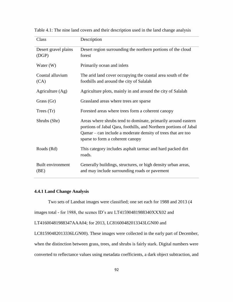
92
Table 4.1: The nine land covers and their description used in the land change analysis
Class Description
Desert gravel plains
(DGP)
Desert region surrounding the northern portions of the cloud
forest
Water (W) Primarily ocean and inlets
Coastal alluvium
(CA)
The arid land cover occupying the coastal area south of the
foothills and around the city of Salalah
Agriculture (Ag) Agriculture plots, mainly in and around the city of Salalah
Grass (Gr) Grassland areas where trees are sparse
Trees (Tr) Forested areas where trees form a coherent canopy
Shrubs (Shr) Areas where shrubs tend to dominate, primarily around eastern
portions of Jabal Qara, foothills, and Northern portions of Jabal
Qamar – can include a moderate density of trees that are too
sparse to form a coherent canopy
Roads (Rd) This category includes asphalt tarmac and hard packed dirt
roads.
Built environment
(BE)
Generally buildings, structures, or high density urban areas,
and may include surrounding roads or pavement
4.4.1 Land Change Analysis
Two sets of Landsat images were classified; one set each for 1988 and 2013 (4
images total - for 1988, the scenes ID’s are LT41590481988340XXX02 and
LT41600481988347AAA04; for 2013, LC81600482013343LGN00 and
LC81590482013336LGN00). These images were collected in the early part of December,
when the distinction between grass, trees, and shrubs is fairly stark. Digital numbers were
converted to reflectance values using metadata coefficients, a dark object subtraction, and
93
climate data records (Masek et al. 2006; USGS 2015). Principle component bands were
calculated and added to the image stack to facilitate classification. An object-based image
analysis method (OBIA; Blaschke 2010) was employed for land cover classification.
Nine land covers were classified (Table 1): desert gravel plains (DGP), water (W),
coastal alluvium (CA), agriculture (Ag), grass (Gr), trees (Tr), Shrubs (Shr), Roads (Rd),
and built environment (BE) (Table 1). The land covers were selected based on field
observations and environmental descriptions in Miller and Morris (1988).
Transition matrices were used to identify systematic land-cover transformation,
which is a conversion from one land cover to another, while accounting for expected
land-cover changes (Pontius et al. 2004). Expected land changes are due to possible
random chance, small changes in large land-cover categories, errors in land-cover maps,
and so on. The transition matrix was developed using the methods outlined in Pontius et
al. (2004) and Alo and Pontius (2008). Observed versus expected land-cover transitions
can be found by analyzing the tradeoffs between land covers as shown in rows and
columns of a transition matrix. Rows of the transition matrix are the land covers as they
stand in 1988 and columns represent the land covers in 2013. Diagonal values show
persistence of land-cover types, while off-diagonal values show the transition from the
land cover for that row (1988) to the land cover for that column (2013). At the end of
each row, a sum shows the total land-cover loss plus persistence as well as the total loss
for that row’s land-cover category. At the end of each column, a sum shows the total
land-cover gain plus the persistence as well as the total gain for that column’s land-cover
category. Expected transitions are calculated by analyzing the observed land-cover gains
and losses and using the formulae in Alo and Pontius (2008; page 288, equations 1 and

94
2). If the observed loss minus the expected loss is positive for a matrix cell, then that
row’s land cover is systematically losing to the land cover in the column; if it is negative,
it is resisting systematic loss. If the observed gain minus the expected gain is positive for
the matrix cell, then that column’s land cover is systematically gaining from the land
cover in the row; if it is negative, it rebuffs systematic gain from the land cover for that
row (Alo and Pontius 2008).
4.4.2 Vegetation Fraction and Subpixel Analysis
Ground covers that occupy varying proportions of a pixel in a satellite image can
be extracted using methods collectively known as subpixel analysis. The basis of this
method lies in the assumption that surface materials may be smaller than the resolution of
the image’s pixel. The surface material proportions within a pixel can be estimated by
using a linear combination of reflectance values of known ground targets, called
endmembers. This approach has been generally termed spectral mixture analysis (SMA;
Settle and Drake 1993), and is often used to model three primary components: vegetation,
impervious surfaces, and soil (V-I-S). It is used here to extract vegetation fraction, a
useful indicator of degradation and deforestation (e.g. Dawelbait and Morari 2012).
Our subpixel approach uses an extension of the SMA method known as multiple
endmember spectral mixture analysis (MESMA; Roberts et al. 1998). MESMA has an
advantage over SMA in that a subset of the total number of endmembers can be modeled
for each pixel, rather than using a linear combination of all endmembers. Three steps are
used to arrive at the endmember proportions (Powell and Roberts 2010). The first step
constructs a library of endmembers. For each endmember, the reflectance values from

95
satellite images are recorded for each band. Finding representative endmembers can be
accomplished using reflectance values from a known spectral library or gathered from
within the image by selecting ‘pure’ pixels (i.e., pixels that are made up almost entirely of
a single endmember). The second step is to construct possible models of endmember
combinations that best fit the known reflectance values at each pixel. To do this, the
endmember proportions must equal 1, each endmember fraction must be constrained
between 0 and 1, and the root mean square error (RMSE) cannot exceed a certain value
(Powell and Roberts 2010). The final step is model selection.
A pixel purity index (PPI; Boardman et al. 1995) finds meaningful endmembers
and was used to construct an endmember library for this study. Over one hundred
possible endmembers were reduced to three primary V-I-S categories, using methods
developed by Dennison and Roberts (2003). Vegetation endmembers were selected
mainly from areas of tree canopy (1988 n=5, 2013 n=23). Impervious surface
endmembers were selected from roads, hard packed dirt tracks, buildings, and desert hard
scrabble (1988 n=7, 2013 n=16). Finally, soil was selected from exposed organic soils in
the cloud forest and coastal alluvium (1988 n=4, 2013 n=4). To arrive at our final
models, we used a four endmember model (V-I-S + shade) and set the RMSE to 0.25.
Any pixels that could not meet the RMSE criteria were masked from our analysis, along
with water pixels and shaded regions.
Since there is no test to determine the statistical significance for the vegetation
fraction, we identified systematic areas of increase and decrease in this fraction by
searching for statistically significant spatial clusters. We determined significant spatial
clusters by using local indicators of spatial association (LISA; Anselin 1995), which

96
organizes pixels of high vegetation fraction (vegetation fraction gains) and pixels of low
vegetation fraction (vegetation fraction losses) into clusters. LISA statistics help
breakdown the global Moran’s I test for spatial autocorrelation into local components.
These local components can be interpreted as spatial clusters or hot spots. The clusters
are tested for significance by using a conditional permutation framework.
4.4.3 Time Series Analysis
One advantage of regularly collected NDVI observations is that these data can be
analyzed using the dynamics of the system over time. The dynamics can be associated
with the mean value observed throughout the year, or the highest value observed, and so
on. Trend analysis was used to determine if key NDVI time series were increasing or
decreasing with time, providing a proxy of ecosystem health (Bai et al. 2008; Hilker
2014). An increase in the trend (positive slope) indicates an NDVI value is getting
stronger with time and implies that net primary production may be increasing. A
decreasing trend (negative slope) indicates and implies the opposite.
Before the trend can be estimated, the yearly observations need to be modeled so
that key parameters can be extracted. We used the seasonal trend analysis methods
outlined in Eastman and others (2009; 2013) to model the mean annual NDVI (referred to
as Amplitude 0) and the NDVI annual cycle (referred to as Amplitude 1). The Amplitude
1 signal is the difference between the minimum and maximum NDVI observations
(Eastman et al. 2013), whereas Amplitude 0 is an average of the annual NDVI signal.
These two observations are extracted by using a harmonic regression to model the yearly
NDVI cycle. A Theil-Sen median slope is then calculated on the Amplitude 0 and 1
97
values for each year. This median slope calculation is robust and can reliably estimate the
trend slope even in the presence of noise and outliers (Theil 1950, Sen 1968). Up to 29%
of the observations can be outliers. Once the slope is calculated, a Mann-Kendal test for
trend significance is created along with z-values, of which we used the z-values to help
determine statistical significance. The NDVI observations were obtained from the
MODIS 16-day NDVI product at 250 m resolution for the years 2001 to 2013 (MODIS
tile 23 horizontal, 7 vertical).
4.5 Results
4.5.1 Transition Matrix
Considerable change in the environment of the cloud forest is revealed (Figure
2.1). Trees had a net loss of about 23,165 ha, and coastal alluvium about 13,469 ha. In
contrast, roads gained about 12,535 ha, the built environment increased by about 9,157
ha, and grass and shrub covers had a net gain of 15,147 ha and 59 ha, respectively. But,
the net gains in shrubs and grasses mask a more complex exchange between land covers.
Tables 4.2 and 4.3 show the transition matrix and a matrix of systematic gains and
losses. According to these matrices, a few land covers systematically transitioned to other
land covers. Despite the large net loss in cover, trees are systematically losing coverage
to only one other land-cover category, shrubs. About 4% of the landscape transitioned
this way (Table 4.2), barely above what was expected from random chance (Table 4.3).
Forest covers resisted transition to roads or the built environment. Only about 0.45% of
the landscape underwent a transition from trees to roads, and even less to the built
environment (0.06%), both well within the expected ranges.

98
Figure 4.1: Land-cover change between 1988 and 2013.
Two land-cover transitions offered some support that infrastructure was driving at
least moderate change. Coastal alluvium lost cover to roads or the built environment
(about 4.5% of the total landscape), a result well beyond expectations (Table 4.3) and a
product of peri-urban expansion. Grass cover also transitioned to road cover above
expectations, occurring mainly in the cloud forest.
The structure of environmental change is registered in the transitions from trees to
shrubs, shrubs to grass, and grass to roads (Tables 4.2 and 4.3). The transition of trees to
shrubs and shrubs to grass hints at a gradual change in vegetation cover as opposed to the
transition of grass to roads, a more abrupt type of change. Tree and shrub covers that
converted to road covers between 1988 and 2013 comprised only about 1% of the
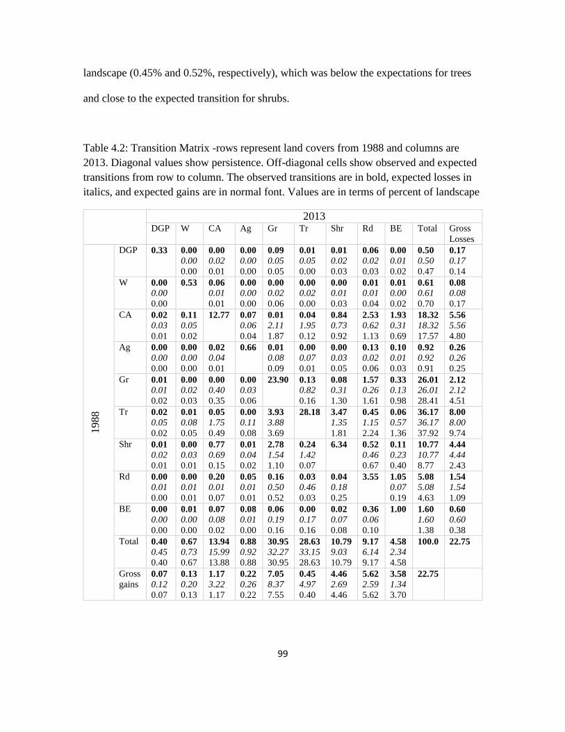
99
landscape (0.45% and 0.52%, respectively), which was below the expectations for trees
and close to the expected transition for shrubs.
Table 4.2: Transition Matrix -rows represent land covers from 1988 and columns are
2013. Diagonal values show persistence. Off-diagonal cells show observed and expected
transitions from row to column. The observed transitions are in bold, expected losses in
italics, and expected gains are in normal font. Values are in terms of percent of landscape
2013 DGP W CA Ag Gr Tr Shr Rd BE Total Gross
Losses
1988
DGP 0.33 0.00
0.00
0.00
0.00
0.02
0.01
0.00
0.00
0.00
0.09
0.05
0.05
0.01
0.05
0.00
0.01
0.02
0.03
0.06
0.02
0.03
0.00
0.01
0.02
0.50
0.50
0.47
0.17
0.17
0.14
W 0.00
0.00
0.00
0.53 0.06
0.01
0.01
0.00
0.00
0.00
0.00
0.02
0.06
0.00
0.02
0.00
0.00
0.01
0.03
0.01
0.01
0.04
0.01
0.00
0.02
0.61
0.61
0.70
0.08
0.08
0.17
CA 0.02
0.03
0.01
0.11
0.05
0.02
12.77 0.07
0.06
0.04
0.01
2.11
1.87
0.04
1.95
0.12
0.84
0.73
0.92
2.53
0.62
1.13
1.93
0.31
0.69
18.32
18.32
17.57
5.56
5.56
4.80
Ag 0.00
0.00
0.00
0.00
0.00
0.00
0.02
0.04
0.01
0.66 0.01
0.08
0.09
0.00
0.07
0.01
0.00
0.03
0.05
0.13
0.02
0.06
0.10
0.01
0.03
0.92
0.92
0.91
0.26
0.26
0.25
Gr 0.01
0.01
0.02
0.00
0.02
0.03
0.00
0.40
0.35
0.00
0.03
0.06
23.90 0.13
0.82
0.16
0.08
0.31
1.30
1.57
0.26
1.61
0.33
0.13
0.98
26.01
26.01
28.41
2.12
2.12
4.51
Tr 0.02
0.05
0.02
0.01
0.08
0.05
0.05
1.75
0.49
0.00
0.11
0.08
3.93
3.88
3.69
28.18 3.47
1.35
1.81
0.45
1.15
2.24
0.06
0.57
1.36
36.17
36.17
37.92
8.00
8.00
9.74
Shr 0.01
0.02
0.01
0.00
0.03
0.01
0.77
0.69
0.15
0.01
0.04
0.02
2.78
1.54
1.10
0.24
1.42
0.07
6.34 0.52
0.46
0.67
0.11
0.23
0.40
10.77
10.77
8.77
4.44
4.44
2.43
Rd 0.00
0.01
0.00
0.00
0.01
0.01
0.20
0.01
0.07
0.05
0.01
0.01
0.16
0.50
0.52
0.03
0.46
0.03
0.04
0.18
0.25
3.55
1.05
0.07
0.19
5.08
5.08
4.63
1.54
1.54
1.09
BE 0.00
0.00
0.00
0.01
0.00
0.00
0.07
0.08
0.02
0.08
0.01
0.00
0.06
0.19
0.16
0.00
0.17
0.16
0.02
0.07
0.08
0.36
0.06
0.10
1.00 1.60
1.60
1.38
0.60
0.60
0.38
Total 0.40
0.45
0.40
0.67
0.73
0.67
13.94
15.99
13.88
0.88
0.92
0.88
30.95
32.27
30.95
28.63
33.15
28.63
10.79
9.03
10.79
9.17
6.14
9.17
4.58
2.34
4.58
100.0
22.75
Gross
gains 0.07
0.12
0.07
0.13
0.20
0.13
1.17
3.22
1.17
0.22
0.26
0.22
7.05
8.37
7.55
0.45
4.97
0.40
4.46
2.69
4.46
5.62
2.59
5.62
3.58
1.34
3.70
22.75
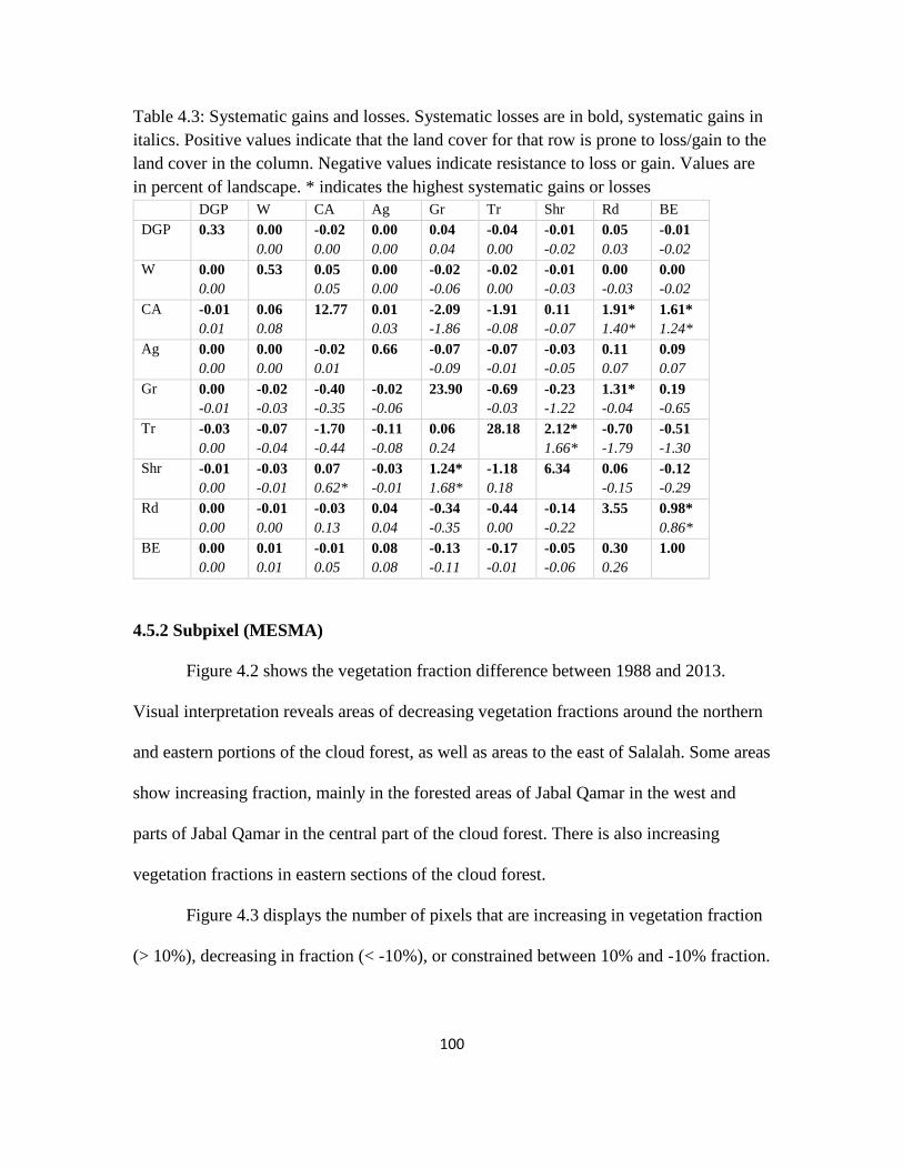
100
Table 4.3: Systematic gains and losses. Systematic losses are in bold, systematic gains in
italics. Positive values indicate that the land cover for that row is prone to loss/gain to the
land cover in the column. Negative values indicate resistance to loss or gain. Values are
in percent of landscape. * indicates the highest systematic gains or losses
DGP W CA Ag Gr Tr Shr Rd BE
DGP 0.33 0.00
0.00
-0.02
0.00
0.00
0.00
0.04
0.04
-0.04
0.00
-0.01
-0.02
0.05
0.03
-0.01
-0.02
W 0.00
0.00
0.53 0.05
0.05
0.00
0.00
-0.02
-0.06
-0.02
0.00
-0.01
-0.03
0.00
-0.03
0.00
-0.02
CA -0.01
0.01
0.06
0.08
12.77 0.01
0.03
-2.09
-1.86
-1.91
-0.08
0.11
-0.07
1.91*
1.40*
1.61*
1.24*
Ag 0.00
0.00
0.00
0.00
-0.02
0.01
0.66 -0.07
-0.09
-0.07
-0.01
-0.03
-0.05
0.11
0.07
0.09
0.07
Gr 0.00
-0.01
-0.02
-0.03
-0.40
-0.35
-0.02
-0.06
23.90 -0.69
-0.03
-0.23
-1.22
1.31*
-0.04
0.19
-0.65
Tr -0.03
0.00
-0.07
-0.04
-1.70
-0.44
-0.11
-0.08
0.06
0.24
28.18 2.12*
1.66*
-0.70
-1.79
-0.51
-1.30
Shr -0.01
0.00
-0.03
-0.01
0.07
0.62*
-0.03
-0.01
1.24*
1.68*
-1.18
0.18
6.34 0.06
-0.15
-0.12
-0.29
Rd 0.00
0.00
-0.01
0.00
-0.03
0.13
0.04
0.04
-0.34
-0.35
-0.44
0.00
-0.14
-0.22
3.55 0.98*
0.86*
BE 0.00
0.00
0.01
0.01
-0.01
0.05
0.08
0.08
-0.13
-0.11
-0.17
-0.01
-0.05
-0.06
0.30
0.26
1.00
4.5.2 Subpixel (MESMA)
Figure 4.2 shows the vegetation fraction difference between 1988 and 2013.
Visual interpretation reveals areas of decreasing vegetation fractions around the northern
and eastern portions of the cloud forest, as well as areas to the east of Salalah. Some areas
show increasing fraction, mainly in the forested areas of Jabal Qamar in the west and
parts of Jabal Qamar in the central part of the cloud forest. There is also increasing
vegetation fractions in eastern sections of the cloud forest.
Figure 4.3 displays the number of pixels that are increasing in vegetation fraction
(> 10%), decreasing in fraction (< -10%), or constrained between 10% and -10% fraction.
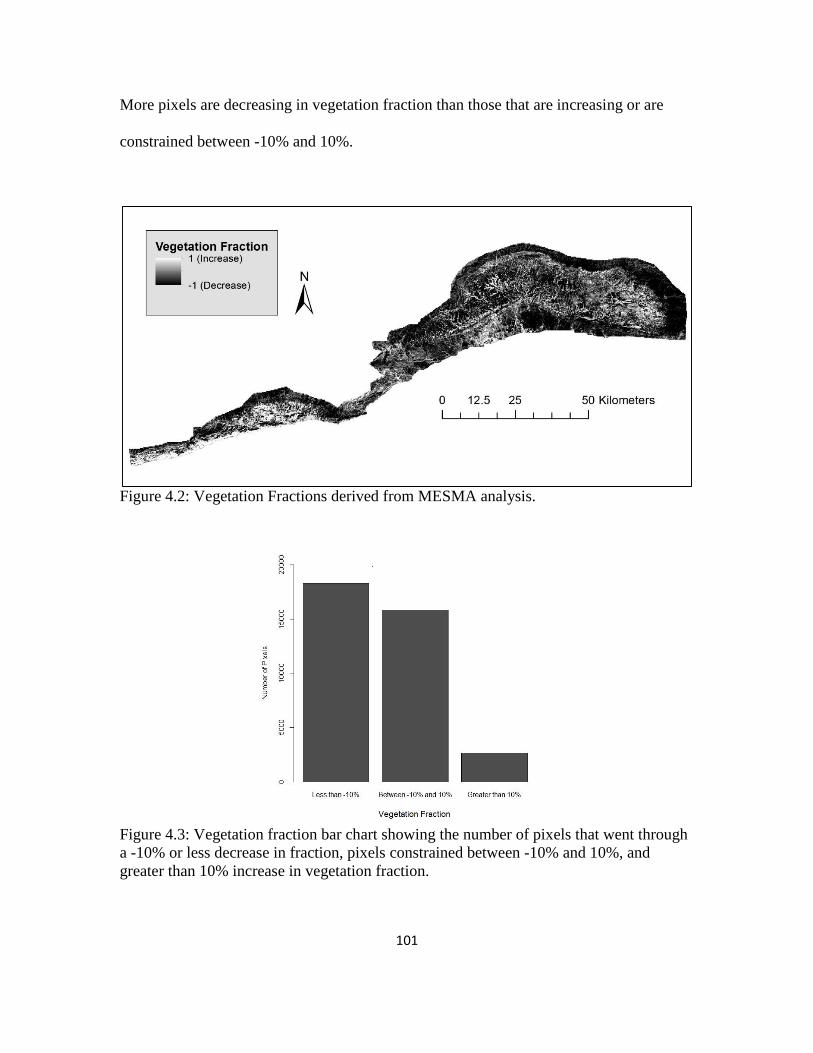
101
More pixels are decreasing in vegetation fraction than those that are increasing or are
constrained between -10% and 10%.
Figure 4.2: Vegetation Fractions derived from MESMA analysis.
Figure 4.3: Vegetation fraction bar chart showing the number of pixels that went through
a -10% or less decrease in fraction, pixels constrained between -10% and 10%, and
greater than 10% increase in vegetation fraction.
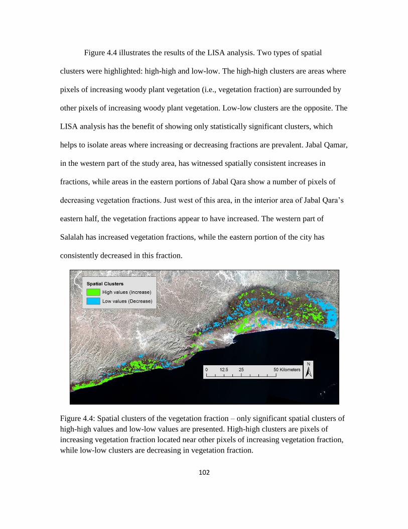
102
Figure 4.4 illustrates the results of the LISA analysis. Two types of spatial
clusters were highlighted: high-high and low-low. The high-high clusters are areas where
pixels of increasing woody plant vegetation (i.e., vegetation fraction) are surrounded by
other pixels of increasing woody plant vegetation. Low-low clusters are the opposite. The
LISA analysis has the benefit of showing only statistically significant clusters, which
helps to isolate areas where increasing or decreasing fractions are prevalent. Jabal Qamar,
in the western part of the study area, has witnessed spatially consistent increases in
fractions, while areas in the eastern portions of Jabal Qara show a number of pixels of
decreasing vegetation fractions. Just west of this area, in the interior area of Jabal Qara’s
eastern half, the vegetation fractions appear to have increased. The western part of
Salalah has increased vegetation fractions, while the eastern portion of the city has
consistently decreased in this fraction.
Figure 4.4: Spatial clusters of the vegetation fraction – only significant spatial clusters of
high-high values and low-low values are presented. High-high clusters are pixels of
increasing vegetation fraction located near other pixels of increasing vegetation fraction,
while low-low clusters are decreasing in vegetation fraction.
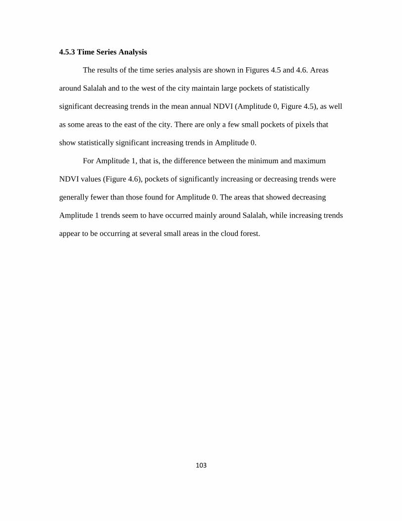
103
4.5.3 Time Series Analysis
The results of the time series analysis are shown in Figures 4.5 and 4.6. Areas
around Salalah and to the west of the city maintain large pockets of statistically
significant decreasing trends in the mean annual NDVI (Amplitude 0, Figure 4.5), as well
as some areas to the east of the city. There are only a few small pockets of pixels that
show statistically significant increasing trends in Amplitude 0.
For Amplitude 1, that is, the difference between the minimum and maximum
NDVI values (Figure 4.6), pockets of significantly increasing or decreasing trends were
generally fewer than those found for Amplitude 0. The areas that showed decreasing
Amplitude 1 trends seem to have occurred mainly around Salalah, while increasing trends
appear to be occurring at several small areas in the cloud forest.

104
Figure 4.5: Amplitude 0 (annual mean NDVI) trend analysis results. The top map shows
the slope of the trend as changes in average NDVI per year (MODIS NDVI = NDVI x
10000). The bottom map shows the z-values used to measure significance (greater than
1.96 or less than -1.96).
105
Figure 4.6: Amplitude 1 (difference between peak and minimum yearly NDVI) trend
analysis results. The top map shows the slope of the trend as changes in peak NDVI per
year (MODIS NDVI = NDVI x 10000). The bottom map shows the z-values used to
measure significance (greater than 1.96 or less than -1.96).

106
4.6 Discussion
4.6.1 Land Changes
The analysis of vegetation fractions suggest there are complex changes occurring
across the study area. Most of the cloud forest area examined witnessed a decrease in
vegetation fraction or minimal change (Figure 4.3). Some areas of the cloud forest,
however, actually increased in vegetation fractions, contradicting the local, prevalent
notion of ubiquitous degradation or deforestation. Several explanations for this increase
are plausible. Increased atmospheric CO2 has been shown to lead to greening in warmer,
arid environments (Donohue et al. 2013)—a phenomenon referred to as the CO2
fertilization effect. Dhofar is one region thought to be experiencing this effect (Figure 2
in Donohue et al. 2013). Another possible reason is shrub encroachment, usually on
grasslands (Asner et al. 2004) and associated with a disturbance to the ecosystem, such as
fires or grazing (Anadón et al. 2014). In the case of Dhofar, shrub encroachment is
generally associated with grazing, because the dominant and most abundant types of
shrubs are those that are unpalatable to livestock (Miller and Morris 1988; Pickering and
Patzelt 2008). Shrub encroachment can have different effects on an ecosystem - it may
possibly lead to both increases and decreases in primary production (Eldridge et al.
2011). Since the transition matrix does not show any systematic transitions between grass
and shrub covers, the shrub encroachment is likely occurring at a level where grasses are
still the dominant land cover, and where shrub encroachment could lead to an increase in
the woody plant fraction (i.e., an increase in the vegetation fraction).
Perhaps the most complex changes are those happening along the coast of Jabal
Qamar. Here, there appears to be places that are increasing in vegetation fraction but
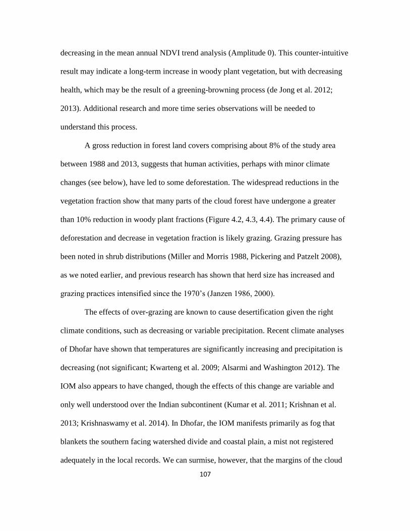
107
decreasing in the mean annual NDVI trend analysis (Amplitude 0). This counter-intuitive
result may indicate a long-term increase in woody plant vegetation, but with decreasing
health, which may be the result of a greening-browning process (de Jong et al. 2012;
2013). Additional research and more time series observations will be needed to
understand this process.
A gross reduction in forest land covers comprising about 8% of the study area
between 1988 and 2013, suggests that human activities, perhaps with minor climate
changes (see below), have led to some deforestation. The widespread reductions in the
vegetation fraction show that many parts of the cloud forest have undergone a greater
than 10% reduction in woody plant fractions (Figure 4.2, 4.3, 4.4). The primary cause of
deforestation and decrease in vegetation fraction is likely grazing. Grazing pressure has
been noted in shrub distributions (Miller and Morris 1988, Pickering and Patzelt 2008),
as we noted earlier, and previous research has shown that herd size has increased and
grazing practices intensified since the 1970’s (Janzen 1986, 2000).
The effects of over-grazing are known to cause desertification given the right
climate conditions, such as decreasing or variable precipitation. Recent climate analyses
of Dhofar have shown that temperatures are significantly increasing and precipitation is
decreasing (not significant; Kwarteng et al. 2009; Alsarmi and Washington 2012). The
IOM also appears to have changed, though the effects of this change are variable and
only well understood over the Indian subcontinent (Kumar et al. 2011; Krishnan et al.
2013; Krishnaswamy et al. 2014). In Dhofar, the IOM manifests primarily as fog that
blankets the southern facing watershed divide and coastal plain, a mist not registered
adequately in the local records. We can surmise, however, that the margins of the cloud
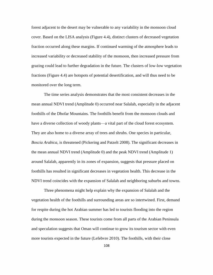
108
forest adjacent to the desert may be vulnerable to any variability in the monsoon cloud
cover. Based on the LISA analysis (Figure 4.4), distinct clusters of decreased vegetation
fraction occurred along these margins. If continued warming of the atmosphere leads to
increased variability or decreased stability of the monsoon, then increased pressure from
grazing could lead to further degradation in the future. The clusters of low-low vegetation
fractions (Figure 4.4) are hotspots of potential desertification, and will thus need to be
monitored over the long term.
The time series analysis demonstrates that the most consistent decreases in the
mean annual NDVI trend (Amplitude 0) occurred near Salalah, especially in the adjacent
foothills of the Dhofar Mountains. The foothills benefit from the monsoon clouds and
have a diverse collection of woody plants—a vital part of the cloud forest ecosystem.
They are also home to a diverse array of trees and shrubs. One species in particular,
Boscia Arabica, is threatened (Pickering and Patzelt 2008). The significant decreases in
the mean annual NDVI trend (Amplitude 0) and the peak NDVI trend (Amplitude 1)
around Salalah, apparently in its zones of expansion, suggests that pressure placed on
foothills has resulted in significant decreases in vegetation health. This decrease in the
NDVI trend coincides with the expansion of Salalah and neighboring suburbs and towns.
Three phenomena might help explain why the expansion of Salalah and the
vegetation health of the foothills and surrounding areas are so intertwined. First, demand
for respite during the hot Arabian summer has led to tourists flooding into the region
during the monsoon season. These tourists come from all parts of the Arabian Peninsula
and speculation suggests that Oman will continue to grow its tourism sector with even
more tourists expected in the future (Lefebvre 2010). The foothills, with their close
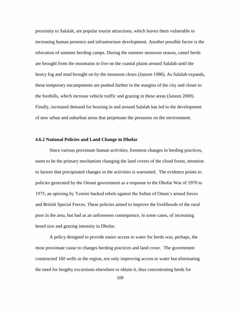
109
proximity to Salalah, are popular tourist attractions, which leaves them vulnerable to
increasing human presence and infrastructure development. Another possible factor is the
relocation of summer herding camps. During the summer monsoon season, camel herds
are brought from the mountains to live on the coastal plains around Salalah until the
heavy fog and mud brought on by the monsoon clears (Janzen 1986). As Salalah expands,
these temporary encampments are pushed further to the margins of the city and closer to
the foothills, which increase vehicle traffic and grazing in these areas (Janzen 2000).
Finally, increased demand for housing in and around Salalah has led to the development
of new urban and suburban areas that perpetuate the pressures on the environment.
4.6.2 National Policies and Land Change in Dhofar
Since various proximate human activities, foremost changes in herding practices,
seem to be the primary mechanism changing the land covers of the cloud forest, attention
to factors that precipitated changes in the activities is warranted. The evidence points to
policies generated by the Omani government as a response to the Dhofar War of 1970 to
1975, an uprising by Yemini backed rebels against the Sultan of Oman’s armed forces
and British Special Forces. These policies aimed to improve the livelihoods of the rural
poor in the area, but had as an unforeseen consequence, in some cases, of increasing
heard size and grazing intensity in Dhofar.
A policy designed to provide easier access to water for herds was, perhaps, the
most proximate cause to changes herding practices and land cover. The government
constructed 160 wells in the region, not only improving access to water but eliminating
the need for lengthy excursions elsewhere to obtain it, thus concentrating herds for
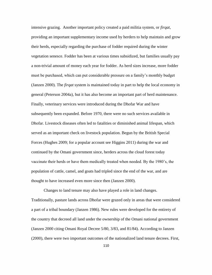
110
intensive grazing. Another important policy created a paid militia system, or firqat,
providing an important supplementary income used by herders to help maintain and grow
their herds, especially regarding the purchase of fodder required during the winter
vegetation senesce. Fodder has been at various times subsidized, but families usually pay
a non-trivial amount of money each year for fodder. As herd sizes increase, more fodder
must be purchased, which can put considerable pressure on a family’s monthly budget
(Janzen 2000). The firqat system is maintained today in part to help the local economy in
general (Peterson 2004a), but it has also become an important part of herd maintenance.
Finally, veterinary services were introduced during the Dhofar War and have
subsequently been expanded. Before 1970, there were no such services available in
Dhofar. Livestock diseases often led to fatalities or diminished animal lifespan, which
served as an important check on livestock population. Begun by the British Special
Forces (Hughes 2009; for a popular account see Higgins 2011) during the war and
continued by the Omani government since, herders across the cloud forest today
vaccinate their herds or have them medically treated when needed. By the 1980’s, the
population of cattle, camel, and goats had tripled since the end of the war, and are
thought to have increased even more since then (Janzen 2000).
Changes to land tenure may also have played a role in land changes.
Traditionally, pasture lands across Dhofar were grazed only in areas that were considered
a part of a tribal boundary (Janzen 1986). New rules were developed for the entirety of
the country that decreed all land under the ownership of the Omani national government
(Janzen 2000 citing Omani Royal Decree 5/80, 3/83, and 81/84). According to Janzen
(2000), there were two important outcomes of the nationalized land tenure decrees. First,
111
camel breeders, who formerly stayed on the fringes of the cloud forest, began to graze
their herds on lands that traditionally belonged to cattle herders; they cited the
nationalized land tenure policy as a rationale for this action. As part of these land tenure
nationalization decrees, the government constructed buildings, schools, and mosques
throughout the cloud forest. This development encouraged the formerly nomadic
population to settle in one place in order to take advantage of the new benefits. As a
result, grazing became more intensive and the traditional transhumance practice is
undertaken mainly by camel herders.
Infrastructure development was a key factor of land change in Dhofar, particularly
around the City of Salalah. The region received about 40% of government expenditures
between 1988 and 2013, much of it for infrastructure development and related projects,
despite only having about 10-25% of the population (Peterson 2004b). More than 4% of
the total study area was converted to urban use around Salalah and other parts of the
coastal plain, and a deep water port was built just outside of Salalah, as well as a paved
road from Salalah to Jabal Qamar (Calvin and Rigsbee 2000). Road development in the
cloud forest led to transitions from grass, shrub, and forest covers to road covers.
Beginning in the 1990’s, existing roads were improved and new roads were constructed
between the coastal plain and the mountains. The new roads are intended to provide
quicker access to the cloud forest or services in Salalah for those living in the mountains.
4.6.3 Land Change Mitigation Factors
While there have been notable changes to the environment of the cloud forest,
common wisdom suggests there has been much more. Part of the reason may reside in
112
Oman’s import of key food staples and the subsequent impact on local cultivation. In the
past, cultivation was more widespread in the cloud forest, possibly as late as the 1970’s
(Janzen 1986). At some point after the 1970’s, cultivation was reduced primarily to small
frankincense plots, walled areas for hay production, or reforestation plots. With Oman’s
oil boom in the late 1960’s, there has been little need to expand cultivation for staple
crops and may have led to a reduction in cropped land as the country imported most of
these foods. Our results suggest little change in cropped land. Dhofar has a strong
tradition of herding rather than farming, and, the critical staples of the Omani diet, like
rice, are increasingly imported rather than grown locally. Imports of rice into Oman
during 2012 totaled about $174 million (OEC 2015).
4.7 Conclusion
The Dhofar cloud forest and coastal plains have witnessed land changes over the
25-year period of this study. These changes have been more complex than local,
commonly expressed views of them entail. Systematic transitions have occurred between
several types of land cover in the cloud forest, primarily tree cover to shrub cover, shrub
cover to grass cover, and grass cover to road cover; while the coastal plains were
systematically transitioning to road cover and the built environment. Vegetation fractions
showed significant clusters of decreasing woody plant cover along the cloud forest
margins and various parts of the coastal plain, and NDVI trend analysis indicates
decreasing NDVI around the city of Salalah since 2001. These changes would appear to
be linked primarily to changes in herding practices and road and peri-urban development,
most of which are linked directly to changes in government policies directed to
113
developing the southern part of Oman. Whether these policies have led to a path
dependent outcome—land-cover trends that are difficult to reverse or alter—remains an
open question.
4.8 Acknowledgements
Support for this research was provided in part by a Fulbright grant to Oman
funded by the U.S. Department of State and sponsored by the Office of the Advisor to
His Majesty The Sultan for Economic Planning Affairs. Special thanks to Dr. Said Al-
Saqri for support during the Fulbright grant period.
4.9 References
Alo, C. A., and R. G. Pontius Jr (2008), Identifying systematic land-cover transitions
using remote sensing and GIS: the fate of forests inside and outside protected areas
of Southwestern Ghana, Environ. Plan. B Plan. Des., 35(2), 280–295,
doi:10.1068/b32091.
AlSarmi, S., and R. Washington (2011), Recent observed climate change over the
Arabian Peninsula, J. Geophys. Res., 116(D11), D11109,
doi:10.1029/2010JD015459.
Anadón, J. D., O. E. Sala, B. L. Turner II, and E. M. Bennett (2014), Effect of woody-
plant encroachment on livestock production in North and South America, Proc.
Natl. Acad. Sci. U. S. A., 111(35), 12948–12953, doi:10.1073/pnas.1320585111.
Anderson, D. M., J. T. Overpeck, and A. K. Gupta (2002), Increase in the Asian
southwest monsoon during the past four centuries., Science, 297(5581), 596–9,
doi:10.1126/science.1072881.
Anselin, L. (1995), Local Indicators of Spatial Association, Geogr. Anal., 27(2), 93–115.
Asner, G. P., A. J. Elmore, L. P. Olander, R. E. Martin, and a. T. Harris (2004), Grazing
Systems, Ecosystem Responses, and Global Change, Annu. Rev. Environ. Resour.,
29(1), 261–299, doi:10.1146/annurev.energy.29.062403.102142.
114
Bai, Z. G., D. L. Dent, L. Olsson, and M. E. Schaepman (2008), Proxy global assessment
of land degradation, Soil Use Manag., 24(3), 223–234, doi:10.1111/j.1475-
2743.2008.00169.x.
Blaschke, T. (2010), Object based image analysis for remote sensing, ISPRS J.
Photogramm. Remote Sens., 65(1), 2–16, doi:10.1016/j.isprsjprs.2009.06.004.
Boardman, J. W., F. A. Kruse, and R. O. Green (1995), Mapping target signatures via
partial unmixing of AVIRIS data, in Summaries of JPL Airborne Earth Science
Workshop, JPL Publication 95-1, pp. 23–26, Pasadena, CA.
Brannstrom, C., and J. M. Vadjunec (2014), Land change science, political ecology and
sustainability: synergies and divergences, edited by C. Brannstrom and J. M.
Vadjunec, Routledge.
Charabi, Y., and S. A. Abdul-Wahab (2009), Synoptic aspects of the summer monsoon of
southern Oman and its global teleconnections, J. Geophys. Res. Atmos., 114(7), 1–9,
doi:10.1029/2008JD010234.
Dawelbait, M., and F. Morari (2012), Monitoring desertification in a Savannah region in
Sudan using Landsat images and spectral mixture analysis, J. Arid Environ., 80, 45–
55, doi:10.1016/j.jaridenv.2011.12.011.
Defries, R. S., T. Rudel, M. Uriarte, and M. Hansen (2010), Deforestation driven by
urban population growth and agricultural trade in the twenty-first century, Nat.
Geosci., 3(3), 178–181, doi:10.1038/ngeo756.
Dennison, P. E., and D. A. Roberts (2003), Endmember selection for multiple
endmember spectral mixture analysis using endmember average RMSE, Remote
Sens. Environ., 87(2-3), 123–135, doi:10.1016/S0034-4257(03)00135-4.
Donohue, R. J., M. L. Roderick, T. R. McVicar, and G. D. Farquhar (2013), Impact of
CO2 fertilization on maximum foliage cover across the globe’s warm, arid
environments, Geophys. Res. Lett., 40(12), 3031–3035, doi:10.1002/grl.50563.
Eastman, J. R., F. Sangermano, B. Ghimire, H. Zhu, H. Chen, N. Neeti, Y. Cai, E. a.
Machado, and S. C. Crema (2009), Seasonal trend analysis of image time series, Int.
J. Remote Sens., 30(10), 2721–2726, doi:10.1080/01431160902755338.
Eastman, J. R., F. Sangermano, E. a. Machado, J. Rogan, and A. Anyamba (2013),
Global trends in seasonality of Normalized Difference Vegetation Index (NDVI),
1982-2011, Remote Sens., 5(10), 4799–4818, doi:10.3390/rs5104799.
Eldridge, D. J., M. a. Bowker, F. T. Maestre, E. Roger, J. F. Reynolds, and W. G.
Whitford (2011), Impacts of shrub encroachment on ecosystem structure and
115
functioning: Towards a global synthesis, Ecol. Lett., 14(7), 709–722,
doi:10.1111/j.1461-0248.2011.01630.x.
Geist, H. J., and E. F. Lambin (2002), Proximate Causes and Underlying Driving Forces
of Tropical Deforestation, Bioscience, 52(2), 143–150.
Ghazanfar, S. (1998), Status of the flora and plant conservation in the sultanate of Oman,
Biol. Conserv., 85(5), 1167–1179.
Gupta, A. K., D. M. Anderson, and J. T. Overpeck (2003), Abrupt changes in the Asian
southwest monsoon during the Holocene and their links to the North Atlantic Ocean,
Nature, 421(6921), 354–7, doi:10.1038/nature01340.
Higgins, A. (2011), With the S.A.S and Other Animals: A Vet’s Experiences During the
Dhofar War 1974, Pen and Sword Books Ltd, Barnsley, UK.
Higuera, D., B. Martín-López, and A. Sánchez-Jabba (2013), Social preferences towards
ecosystem services provided by cloud forests in the neotropics: Implications for
conservation strategies, Reg. Environ. Chang., 13(4), 861–872, doi:10.1007/s10113-
012-0379-1.
Hildebrandt, A. (2005), Ecohydrology of a Seasonal Cloud Forest in Dhofar, PhD.
Dissertation, Massachusetts Institute of Technology.
Hildebrandt, A., and E. A. B. Eltahir (2006), Forest on the edge: Seasonal cloud forest in
Oman creates its own ecological niche, Geophys. Res. Lett., 33(11), 2–5,
doi:10.1029/2006GL026022.
Hildebrandt, A., and E. a. B. Eltahir (2007), Ecohydrology of a seasonal cloud forest in
Dhofar: 2. Role of clouds, soil type, and rooting depth in tree-grass competition,
Water Resour. Res., 43(11), n/a–n/a, doi:10.1029/2006WR005262.
Hilker, T., E. Natsagdorj, R. H. Waring, A. Lyapustin, and Y. Wang (2014), Satellite
observed widespread decline in Mongolian grasslands largely due to overgrazing,
Glob. Chang. Biol., 20(2), 418–28.
Hughes, G. (2009), A “Model Campaign” Reappraised: The Counter-Insurgency War in
Dhofar, Oman, 1965–1975, J. Strateg. Stud., 32(2), 271–305,
doi:10.1080/01402390902743357.
Janzen, J. (1986), Nomads in the sultanate of Oman: tradition and development in
Dhofar, Westview Press, Boulder.
116
Janzen, J. (2000), The destruction of resources among the mountain nomads of Dhofar, in
The Transformation of Nomadic Society in the Arab East, edited by M. Mundy and
B. Musallam, pp. 160–175, Cambridge University Press, Cambridge, UK.
De Jong, R., J. Verbesselt, M. E. Schaepman, and S. de Bruin (2012), Trend changes in
global greening and browning: Contribution of short-term trends to longer-term
change, Glob. Chang. Biol., 18(2), 642–655, doi:10.1111/j.1365-
2486.2011.02578.x.
De Jong, R., J. Verbesselt, A. Zeileis, and M. E. Schaepman (2013), Shifts in global
vegetation activity trends, Remote Sens., 5(3), 1117–1133, doi:10.3390/rs5031117.
Krishnan, R., T. P. Sabin, D. C. Ayantika, a. Kitoh, M. Sugi, H. Murakami, a. G. Turner,
J. M. Slingo, and K. Rajendran (2013), Will the South Asian monsoon overturning
circulation stabilize any further?, Clim. Dyn., 40(1-2), 187–211,
doi:10.1007/s00382-012-1317-0.
Krishnaswamy, J., S. Vaidyanathan, B. Rajagopalan, M. Bonell, M. Sankaran, R. S.
Bhalla, and S. Badiger (2014), Non-stationary and non-linear influence of ENSO
and Indian Ocean Dipole on the variability of Indian monsoon rainfall and extreme
rain events, Clim. Dyn., doi:10.1007/s00382-014-2288-0.
Kumar, K. K., B. Rajagopalan, M. Hoerling, G. Bates, and M. Cane (2006), Unraveling
the mystery of Indian monsoon failure during El Niño, Science, 314(5796), 115–
119.
Kumar, K. K., K. Kamala, B. Rajagopalan, M. P. Hoerling, J. K. Eischeid, S. K.
Patwardhan, G. Srinivasan, B. N. Goswami, and R. Nemani (2011), The once and
future pulse of Indian monsoonal climate, Clim. Dyn., 36(11-12), 2159–2170,
doi:10.1007/s00382-010-0974-0.
Kwarteng, A. Y., S. Dorvlo, and G. T. V. Kumar (2009), Analysis of a 27-year rainfall
data (1977 – 2003) in the Sultanate of Oman, Int. J. Climatol., 617(July 2008), 605–
617, doi:10.1002/joc.
Lambin, E. F., B. L. Turner, H. J. Geist, S. B. Agbola, A. Angelsen, J. Bruce, O. Coomes,
R. Dirzo, G. Fischer, and C. Folke (2001), The causes of land-use and land-cover
change: moving beyond the myths, Glob. Environ. Chang., 11(4), 261–269,
doi:10.1016/S0959-3780(01)00007-3.
Lambin, E. F., H. J. Geist, and E. Lepers (2003), Dynamics of Land-Use and Land-Cover
Change in Tropical Regions, Annu. Rev. Environ. Resour., 28(1), 205–241.
Lefebvre, J. A. (2010), Oman’s Foreign Policy in the Twenty-First Century, Middle East
Policy, 17(1), 99–114.
117
Li, S., P. H. Verburg, L. Shihai, J. Wu, and X. Li (2012), Spatial analysis of the driving
factors of grassland degradation under conditions of climate change and intensive
use in Inner Mongolia, China, Reg. Environ. Chang., 12(3), 461–474,
doi:10.1007/s10113-011-0264-3.
Liu, J. et al. (2013), Framing Sustainability in a Telecoupled World, Ecol. Soc., 18(2), 26,
doi:10.5751/ES-05873-180226.
Masek, J. G., E. F. Vermote, N. E. Saleous, R. Wolfe, F. G. Hall, K. F. Huemmrich, F.
Gao, J. Kutler, and T. Lim (2006), A Landsat Surface Reflectance Dataset for North
America, 1990-2000, IEEE Geosci. Remote Sens. Lett., 3(1), 68–72,
doi:10.1109/LGRS.2005.857030.
Miller, A. G., and M. Morris (1988), Plants of Dhofar, the southern region of Oman,
traditional, economic and medicinal uses, Office of the Adviser for Conservation of
the Environment, Diwan of Royal Court, Sultanate of Oman.
O’Reilly, M. J. (1998), Omanibalancing: Oman Confronts an Uncertain Future, Middle
East J., 52(1), 70–84.
OEC (2015), Observatory of Economic Complexity, Available from:
https://atlas.media.mit.edu/en/ (Accessed 1 May 2015)
Patzelt, A. (2011), The Themeda Quadrivalvis Tall-Grass Savannah of Oman At the
Crossroad Between Africa and Asia, Edinburgh J. Bot., 68(02), 301–319,
doi:10.1017/S0960428611000217.
Peterson, J. E. (2004a), Oman: Three and a Half Decades Of Change and Development,
Middle East Policy, XI(2), 125–137.
Peterson, J. E. (2004b), Oman’s Diverse Society : Southern Oman, Middle East J., 58(1),
31–51.
Peterson, J. E. (2011), Oman Faces the Twenty-First Century, in Political Change in the
Arab Gulf States: Stuck in Transition, edited by M. A. Tétreault, G. Okruhlik, and
A. Kapiszewski, pp. 99–118, Lynne Rienner Publishers, Boulder.
Pickering, H. A., and A. Patzelt (2008), Field Guide to the Wild Plants of Oman, Kew
Publishing, Richmond, UK.
Pontius, R. G., E. Shusas, and M. McEachern (2004), Detecting important categorical
land changes while accounting for persistence, Agric. Ecosyst. Environ., 101(2-3),
251–268, doi:10.1016/j.agee.2003.09.008.
118
Powell, R. L., and D. A. Roberts (2010), Characterizing Urban Land-Cover Change in
Rondônia, Brazil: 1985 to 2000, J. Lat. Am. Geogr.
Roberts, D., M. Gardner, R. Church, S. Ustin, G. Scheer, and R. Green (1998), Mapping
Chaparral in the Santa Monica Mountains Using Multiple Endmember Spectral
Mixture Models, Remote Sens. Environ., 65(3), 267–279, doi:10.1016/S0034-
4257(98)00037-6.
Scholte, P., and P. De Geest (2010), The climate of Socotra Island (Yemen): A first-time
assessment of the timing of the monsoon wind reversal and its influence on
precipitation and vegetation patterns, J. Arid Environ., 74(11), 1507–1515,
doi:10.1016/j.jaridenv.2010.05.017.
Sen, P. K. (1968), Estimates of the regression coefficient based on Kendall’s tau, J. Am.
Stat. Assoc., 63, 1379–1389.
Serneels, S., and E. F. Lambin (2001), Proximate causes of land-use change in Narok
District, Kenya: a spatial statistical model, Agric. Ecosyst. Environ., 85(1-3), 65–81,
doi:10.1016/S0167-8809(01)00188-8.
Seto, K. C., and A. Reenberg (2014), Rethinking global land use in an urban era, edited
by K. C. Seto and A. Reenberg, MIT Press, Cambridge.
Settle, J. J., and N. A. Drake (1993), Linear mixing and the estimation of ground cover
proportions, Int. J. Remote Sens., 14(6), 1159–1177.
Theil, H. (1950), A rank-invariant method of linear and polynomial regression analysis, I,
II, III, Proc. K. Ned. Acad. van Wet., 53(386), 386–392, 512–525, 1397–1412.
Turner II, B. L., E. F. Lambin, and A. Reenberg (2007), Land Change Science Special
Feature: The emergence of land change science for global environmental change and
sustainability, Proc. Natl. Acad. Sci. U. S. A., 104(52), 20666–20671,
doi:10.1073/pnas.0704119104.
UNEP (1994), United Nations Convention to Combat Desertification in those Countries
Experiencing Serious Drought and/or Desertification, Particularly in Africa.
USGS (2015), Product Guide: Landsat 4-7 Climate Data Record (CDR) Surface
Reflectance v. 5.8.
Vayda, A. P., and B. B. Walters (1999), Against political ecology, Hum. Ecol., 27(1),
167–179, doi:10.1023/A:1018713502547.
119
CHAPTER 5
CONCLUSIONS
5.1 Summary and Key Findings
Chapters 2, 3, and 4 provide the first systematic treatment of vegetation patterns
and changes in the Dhofar cloud forest, linking various potential drivers to the changes
observed. The results show that an answer to the question “what drives environmental
change in Dhofar’s cloud forest” is not easy to ascertain. It has long been thought that the
environment in Dhofar is under stress from human and climatic influences. The studies
presented in this dissertation attempt to unfurl the role of both influence and shed light on
biodiversity across the cloud forest.
Chapter 2 was a study of ISM dynamics and its effects on NDVI time series for
the cloud forest in Dhofar. The findings of this chapter provide compelling evidence that,
while the timing and severity of the monsoon is variable, the cloud forest vegetation is
rather robust to these variations, showing only weak to moderate correlations with June
precipitation, and the area under the curve (AUC) of monsoon maximum daily
temperatures. One factor proposed to maintain a strong influence, length of the monsoon,
did not show any meaningful relationship to vegetation dynamics. The strongest driver of
vegetation dynamics was SST in the Arabian Sea. Based on a linear time series model,
SST is about six to nine months out of phase with NDVI measurements in the cloud
forest. Previous research has shown that the presence of cloud cover is a key determinant
in lowering evapotranspiration and providing precipitation that is not accurately
measured by rain gauges or in climate station archives (Hildebrandt 2005; Hildebrandt
120
and Eltahir 2006; Hildebrandt et al. 2007; Hildebrandt and Eltahir 2007). Chapter 2
confirms the importance of cloud cover, both in determining the timing of the ISM and
the importance it plays in shielding the vegetation from monsoon variation. While there is
no evidence that climate changes have affected the cloud forest vegetation, a potential
vulnerability exists: any destabilization of the upwelling that leads to cloud formation
over southern Arabia could cause problems for the cloud forest.
Chapter 3 describes the vegetation diversity of the Dhofar cloud forest, and
reconciles three possible mechanisms of biodiversity: (H1) neutral processes, (H2)
biological interactions, and (H3) environmental gradients. Th biological interactions
hypothesis has the most support in terms of explaining biodiversity. A cluster analysis
showed two dominant groups of tree and shrub species in the cloud forest. A further
analysis of species abundances shows that A. dhofarica and Commiphora spp. make-up
almost 50% of the overall relative abundances in forested areas, and C. procera,
Commiphora spp., and S. incanum make-up about 42% of relative species abundances in
grassland areas. Species abundances (especially A. dhofarica and Commiphora spp.)
suggest that the biogeographical history has played a role in today’s biodiversity patterns
in the forested areas. The cloud forest is a remnant of an ancient forest that developed
during the Tertiary, and was thought to spread across the modern pan-Indian ocean
region. Today, the endemic and non-endemic species that comprise the cloud forest show
strong affinities with plant communities in Africa and India. The fact that these same
species dominate the cloud forest’s biodiversity patterns suggests that the Dhofar
Mountains are an important refuge, and will be so for a long time to come. The
grasslands show signs of human influence; the proliferation of C. procera and S. incanum

121
are a testament to the prevalence of livestock. These two species are known to be
poisonous to livestock and thrive in areas where grazing is common, suggesting that
human activities play a strong role in shaping biodiversity patterns as well.
Using a variety of methods to understand the extent of human influence on the
environment, Chapter 4 shows that the Dhofar War has a strong legacy in transforming
land use and thus land cover of the cloud forest and coastal region. The link between the
Dhofar War and the environment is strongest in certain policies. Foremost among these
are investments made in Dhofar’s infrastructure and several policies put in place to
improve the well-being of local inhabitants. The decision to invest heavily in Dhofar was
a necessary compromise to end the war and cement the union between Dhofar and the
rest of Oman. These policies helped to increase herd size, which eventually led to
overgrazing and about 23,000 ha of deforestation. The infrastructure investments led to
an additional 124 km2 of buildings and roads added to the city of Salalah between 1988
and 2013. The impact of these new roads and urban development has been widespread
and signs of stress to the coastal land cover are commonplace, particularly in the 21st
century. Dhofar is now an example of the trade-off between human well-being and
environmental degradation.
5.2 Reconciling the Role of Humans and Climate as Agents of Change
What role does climate and human impacts have on changing the cloud forest?
The answer to this question appears clearer based on the finding from Chapters 2, 3, and
4. While the monsoon varies from year to year, the strongest evidence for the cause of
environmental change points toward human activities. The evidence from a land change

122
model between 1988 and 2013, plus the MESMA and NDVI time series analyses point to
one conclusion: humans are actively transforming the environment in Dhofar. While
others have predicted the role of humans as an agent of change within Dhofar’s cloud
forest (Janzen 1986), the results in this dissertation provide the first quantitative evidence
for this to date.
Understanding the role of humans in transforming the environment in Dhofar
would not have been possible without a thorough examination of the climate. Global
change research encompasses many different fields of inquiry. As researchers bring
specialized knowledge to bear on environmental change problems, it is critical that the
various threads of change be delineated and defined. Climate change has already
transformed the Earth system, and will continue to do so for some time to come. Human
activities have also transformed the Earth system through such activities as deforestation,
land degradation, and urbanization. As this dissertation has demonstrated, claims about
the cause of change require a thorough examination to decipher the actual role of climate
and human modification.
Common wisdom in Dhofar suggests that the monsoon was changing and with it
the environment. Common wisdom also suggests that grazing and development caused
deforestation and land degradation. Before either of these claims could be examined in
detail, it was necessary to reconcile each with a dedicated study. While Chapters 2, 3, and
4 show that human activity is largely responsible for the land cover changes identified.
Perhaps over the longer-haul, global warming will affect the deep ocean layers of water
and thus the circulation that drives the monsoon. For now, however, this change has a
human imprint.
123
Framing questions of environmental change to incorporate the range of possible
drivers and feedbacks requires both a global and local perspective (Harden 2012).
Systemic changes to the Earth system can have local effects (i.e., climate changes), and
local environmental changes (i.e., land use and covers) can accumulate and work as an
aggregate force of change to the Earth system (Turner et al. 1990). This study sought to
navigate between the systemic and cumulative attributes of environmental change,
seeking which has had the most impact of the Dhofar cloud forest, within insights that
may prove useful for other monsoon driven cloud forests in arid lands.
5.3 Contributions to Scientific Knowledge
This dissertation offers three broad contributions to research and outreach. First, it
contributes to the efforts of land system science to monitor and understand land-cover
changes, especially of sensitive ecosystems (Turner et al. 2007). In this case, this study
demonstrates how to employ multiple platforms and sensors to detect and understand
changes and the role of climate variability on vegetation dynamics. Second, it provides
foundational data of interest to local decision makers and environmental-sustainability
organizations interested in the preservation of the Dhofar cloud forest and the
environmental services it provides. Lastly, this research offers perspectives on
biodiversity and broader forces of land-cover change.
Most research on the ISM is studied through the lens of the Indian subcontinent.
There have been few studies that address the ISM over southern Arabia, and fewer still
that address the relationship between the monsoon and the cloud forest. Chapter 2 is the
first study of its kind to attempt to develop a model of the timing of the monsoon over the
124
Arabian Peninsula. This chapter also develops a time series model of monsoon and
vegetation dynamics. Cloud forests have been shown to be important centers of
endemism and biodiversity. Chapter 2 contributes to knowledge about cloud forests by
showing that they are robust to most climate fluctuations, with the exception of cloud
cover and fog moisture. As such, the study of cloud forests and climate change should
focus on how climate changes may affect the mechanisms of cloud formation and how
this can be affected by future climate changes.
The analysis of cloud forest trees and shrubs in Chapter 3 offers interesting
findings on how biological interactions can lead to dominance by a few species in cloud
forest biodiversity. Perhaps what is most intriguing about this study is that both forests
and grasslands show dominance by a small group of species, but possibly for different
reasons. The study suggests that humans drive biodiversity patterns in the grasslands,
while biogeographical history drives diversity in the forested areas. Few, if any studies,
have suggested such when looking at a cohesive ecosystem.
Finally, the three models developed to study land change in Dhofar show how
multiple methods can be combined to study how humans are altering landscapes.
Commonly, land change is studied through the lens of a single model. But as Chapter 4
demonstrates, a subpixel analysis (MESMA), a land change model (the transition model),
and time series analysis can be combined to study the way various aspects of an
environment are changing. This study also details how national policies following the
Dhofar War in the 1970’s influence development patterns, and ultimately land change.
Thus, it joins others in indicating how “distal” drivers operate on land use and thus land
cover. Specifically, this study hints that there will be significant difficulties implementing

125
policies to mitigate overgrazing and deforestation in the Dhofar cloud forest because the
very policies that increase human well-being have led to environmental degradation.
126
REFERENCES
Abdul-Wahab, S. A., H. Al-Hinai, K. A. Al-Najar, and M. S. Al-Kalbani (2007), Fog
Water Harvesting: Quality of Fog Water Collected for Domestic and Agricultural
Use, Environ. Eng. Sci., 24(4), 446–456, doi:10.1089/ees.2006.06-0066.
Allan, R., D. Chambers, W. Drosdowsky, H. Hendon, M. Latif, N. Nicholls, I. Smith, R.
Stone, and Y. Tourre (2001), Is there an Indian Ocean dipole, and is it independent
of the El Niño - Southern Oscillation?, Clivar Exch., 6(3), 18–22.
Alo, C. A., and R. G. Pontius Jr (2008), Identifying systematic land-cover transitions
using remote sensing and GIS: the fate of forests inside and outside protected areas
of Southwestern Ghana, Environ. Plan. B Plan. Des., 35(2), 280–295,
doi:10.1068/b32091.
AlSarmi, S., and R. Washington (2011), Recent observed climate change over the
Arabian Peninsula, J. Geophys. Res., 116(D11), D11109,
doi:10.1029/2010JD015459.
Anadón, J. D., O. E. Sala, B. L. Turner II, and E. M. Bennett (2014), Effect of woody-
plant encroachment on livestock production in North and South America, Proc.
Natl. Acad. Sci. U. S. A., 111(35), 12948–12953, doi:10.1073/pnas.1320585111.
Anderson, D. M., J. T. Overpeck, and A. K. Gupta (2002), Increase in the Asian
southwest monsoon during the past four centuries, Science, 297(5581), 596–599.
Anselin, L. (1995), Local Indicators of Spatial Association, Geogr. Anal., 27(2), 93–115.
Anyamba, A., C. J. Tucker, and J. R. Eastman (2001), NDVI anomaly patterns over
Africa during the 1997 / 98 ENSO warm event, Intern. J. Remote Sens., 22(10),
1847–1859.
Archer, E. (2004), Beyond the “climate versus grazing” impasse: using remote sensing to
investigate the effects of grazing system choice on vegetation cover in the eastern
Karoo, J. Arid Environ., 57(3), 381–408, doi:10.1016/S0140-1963(03)00107-1.
Ashok, K., Z. Guan, and T. Yamagata (2001), Impact of the Indian Ocean Dipole on the
Relationship between the Indian Monsoon Rainfall and ENSO, Geophys. Res. Lett.,
28(23), 4499–4502, doi:10.1029/2001GL013294.
Ashok, K., Z. Guan, N. H. Sagi, and T. Yagamata (2004), Individual and Combined
influences of ENSO and the\rIndian Ocean Dipole on the Indian Summer Monsoon,
J. Clim., 17(16), 3141–3155, doi:10.1175/1520-
0442(2004)017<3141:IACIOE>2.0.CO;2.
127
Asner, G. P., A. J. Elmore, L. P. Olander, R. E. Martin, and a. T. Harris (2004), Grazing
Systems, Ecosystem Responses, and Global Change, Annu. Rev. Environ. Resour.,
29(1), 261–299, doi:10.1146/annurev.energy.29.062403.102142.
Bai, Z. G., D. L. Dent, L. Olsson, and M. E. Schaepman (2008), Proxy global assessment
of land degradation, Soil Use Manag., 24(3), 223–234, doi:10.1111/j.1475-
2743.2008.00169.x.
Berhane, A., Ø. Totland, M. Haile, and S. R. Moe (2015), Intense use of woody plants in
a semiarid environment of Northern Ethiopia: Effects on species composition,
richness and diversity, J. Arid Environ., 114, 14–21,
doi:10.1016/j.jaridenv.2014.11.001.
De Beurs, K. M., and G. M. Henebry (2010), Spatio-Temporal Statistical Methods for
Modelling Land Surface Phenology, in Phenological Research, edited by I. L.
Hudson and M. R. Keatley, pp. 177–208, Springer Netherlands.
Blaschke, T. (2010), Object based image analysis for remote sensing, ISPRS J.
Photogramm. Remote Sens., 65(1), 2–16, doi:10.1016/j.isprsjprs.2009.06.004.
Blechschmidt, I., A. Matter, F. Preusser, and D. Rieke-Zapp (2009), Monsoon triggered
formation of Quaternary alluvial megafans in the interior of Oman, Geomorphology,
110(3-4), 128–139, doi:10.1016/j.geomorph.2009.04.002.
Boardman, J. W., F. A. Kruse, and R. O. Green (1995), Mapping target signatures via
partial unmixing of AVIRIS data, in Summaries of JPL Airborne Earth Science
Workshop, JPL Publication 95-1, pp. 23–26, Pasadena, CA.
Borcard, D., and P. Legendre (2012), Is the Mantel correlogram powerful enough to be
useful in ecological analysis? A simulation study, Ecology, 93(6), 1473–1481,
doi:10.1890/11-1737.1.
Borcard, D., F. Gillet, and P. Legendre (2011), Numerical Ecology with R, Springer, New
York.
Brannstrom, C., and J. M. Vadjunec (2014), Land change science, political ecology and
sustainability: synergies and divergences, edited by C. Brannstrom and J. M.
Vadjunec, Routledge.
Burns, S. J., D. Fleitmann, A. Matter, U. Neff, and A. Mangini (2001), Speleothem
evidence from Oman for continental pluvial events during interglacial periods,
Geology, 29(7), 623, doi:10.1130/0091-7613(2001)029<0623:SEFOFC>2.0.CO;2.
Charabi, Y. (2009), Arabian summer monsoon variability: Teleconexion to ENSO and
IOD, Atmos. Res., 91(1), 105–117, doi:10.1016/j.atmosres.2008.07.006.
128
Charabi, Y., and S. A. Abdul-Wahab (2009), Synoptic aspects of the summer monsoon of
southern Oman and its global teleconnections, J. Geophys. Res. Atmos., 114(7), 1–9,
doi:10.1029/2008JD010234.
Chisholm, R. A., and S. W. Pacala (2010), Niche and neutral models predict
asymptotically equivalent species abundance distributions in high-diversity
ecological communities., Proc. Natl. Acad. Sci. U. S. A., 107(36), 15821–5,
doi:10.1073/pnas.1009387107.
Condit, R. et al. (2002), Beta-diversity in tropical forest trees, Science, 295(5555), 666–9,
doi:10.1126/science.1066854.
Cook, B. I., R. L. Miller, and R. Seager (2009), Amplification of the North American
“Dust Bowl” drought through human-induced land degradation, Proc. Natl. Acad.
Sci. U. S. A., 106(13), 4997–5001, doi:10.1073/pnas.0810200106.
Cook, E. R., D. M. Meko, D. W. Stahle, and M. K. Cleaveland (1999), Drought
Reconstructions for the Continental United States, J. Clim., 12, 1145–1163.
Cremaschi, M., and F. Negrino (2005), Evidence for an abrupt climatic change at 8700
14C yr B.P. in rockshelters and caves of Gebel Qara (Dhofar-Oman):
Palaeoenvironmental implications, Geoarchaeology, 20(6), 559–579,
doi:10.1002/gea.20068.
Dauby, G., O. J. Hardy, M. Leal, F. Breteler, and T. Stévart (2014), Drivers of tree
diversity in tropical rain forests: new insights from a comparison between littoral
and hilly landscapes of Central Africa, edited by P. Linder, J. Biogeogr., 41(3), 574–
586, doi:10.1111/jbi.12233.
Dawelbait, M., and F. Morari (2012), Monitoring desertification in a Savannah region in
Sudan using Landsat images and spectral mixture analysis, J. Arid Environ., 80, 45–
55, doi:10.1016/j.jaridenv.2011.12.011.
DeFries, R., and D. Pandey (2010), Urbanization, the energy ladder and forest transitions
in India’s emerging economy, Land use policy, 27(2), 130–138,
doi:10.1016/j.landusepol.2009.07.003.
Defries, R. S., T. Rudel, M. Uriarte, and M. Hansen (2010), Deforestation driven by
urban population growth and agricultural trade in the twenty-first century, Nat.
Geosci., 3(3), 178–181, doi:10.1038/ngeo756.
Dennison, P. E., and D. A. Roberts (2003), Endmember selection for multiple
endmember spectral mixture analysis using endmember average RMSE, Remote
Sens. Environ., 87(2-3), 123–135, doi:10.1016/S0034-4257(03)00135-4.
129
Donohue, R. J., M. L. Roderick, T. R. McVicar, and G. D. Farquhar (2013), Impact of
CO2 fertilization on maximum foliage cover across the globe’s warm, arid
environments, Geophys. Res. Lett., 40(12), 3031–3035, doi:10.1002/grl.50563.
Eastman, J. R., F. Sangermano, B. Ghimire, H. Zhu, H. Chen, N. Neeti, Y. Cai, E. a.
Machado, and S. C. Crema (2009), Seasonal trend analysis of image time series, Int.
J. Remote Sens., 30(10), 2721–2726, doi:10.1080/01431160902755338.
Eastman, J. R., F. Sangermano, E. a. Machado, J. Rogan, and A. Anyamba (2013),
Global trends in seasonality of Normalized Difference Vegetation Index (NDVI),
1982-2011, Remote Sens., 5(10), 4799–4818, doi:10.3390/rs5104799.
Eldridge, D. J., M. a. Bowker, F. T. Maestre, E. Roger, J. F. Reynolds, and W. G.
Whitford (2011), Impacts of shrub encroachment on ecosystem structure and
functioning: Towards a global synthesis, Ecol. Lett., 14(7), 709–722,
doi:10.1111/j.1461-0248.2011.01630.x.
Fairhead, J., and M. Leach (1996), Misreading the African landscape: Society and
ecology in a forest-savanna mosaic, Cambridge University Press.
Fasullo, J., and P. J. Webster (2003), A hydrological definition of Indian Monsoon onset
and withdrawal, J. Clim., 16(19), 3200–3211, doi:10.1175/1520-
0442(2003)016<3200a:AHDOIM>2.0.CO;2.
Fieux, M., and H. Stommel (1977), Onset of the Southwest Monsoon over the Arabian
Sea from Marine Reports of Surface Winds: Structure and Variability, Mon.
Weather Rev., 105(2), 231–236.
Flagg, C. N., and H. S. Kim (1998), Upper ocean currents in the northern Arabian Sea
from shipboard ADCP measurements collected during the 1994-1996 U.S. JGOFS
and ONR programs, Deep. Res. Part II Top. Stud. Oceanogr., 45(10-11), 1917–
1959, doi:10.1016/S0967-0645(98)00059-9.
Fleitmann, D., and A. Matter (2009), The speleothem record of climate variability in
Southern Arabia, Comptes Rendus Geosci., 341(8-9), 633–642,
doi:10.1016/j.crte.2009.01.006.
Fleitmann, D., S. J. Burns, M. Mudelsee, U. Neff, J. Kramers, A. Mangini, and A. Matter
(2003), Holocene forcing of the Indian monsoon recorded in a stalagmite from
southern Oman, Science (80-. )., 300(5626), 1737–1739,
doi:10.1126/science.1083130.
Fleitmann, D., S. J. Burns, U. Neff, M. Mudelsee, A. Mangini, and A. Matter (2004),
Palaeoclimatic interpretation of high-resolution oxygen isotope profiles derived

130
from annually laminated speleothems from Southern Oman, Quat. Sci. Rev., 23(7-8),
935–945, doi:10.1016/j.quascirev.2003.06.019.
Fleitmann, D., S. J. Burns, M. Pekala, A. Mangini, A. Al-Subbary, M. Al-Aowah, J.
Kramers, and A. Matter (2011), Holocene and Pleistocene pluvial periods in Yemen,
southern Arabia, Quat. Sci. Rev., 30(7-8), 783–787,
doi:10.1016/j.quascirev.2011.01.004.
Geist, H. J., and E. F. Lambin (2002), Proximate Causes and Underlying Driving Forces
of Tropical Deforestation, Bioscience, 52(2), 143–150.
Ghazanfar, S. (1998), Status of the flora and plant conservation in the sultanate of Oman,
Biol. Conserv., 85(3), 287–295, doi:10.1016/S0006-3207(97)00162-6.
Ghazanfar, S. A., and M. Fisher (eds) (1998), Vegetation of the Arabian Peninsula, edited
by S. A. Ghazanfar and M. Fisher, Kluwer Academic Publishers, Dordrecht.
Goswami, B. N., and R. S. A. Mohan (2001), Intraseasonal oscillations and interannual
variability of the Indian summer monsoon, J. Clim., 14(6), 1180–1198.
Grau, H. R., R. Torres, N. I. Gasparri, P. G. Blendinger, S. Marinaro, and L. Macchi
(2014), Natural grasslands in the Chaco. A neglected ecosystem under threat by
agriculture expansion and forest-oriented conservation policies, J. Arid Environ., (in
press), doi:10.1016/j.jaridenv.2014.12.006.
Gupta, A. K., D. M. Anderson, and J. T. Overpeck (2003), Abrupt changes in the Asian
southwest monsoon during the Holocene and their links to the North Atlantic Ocean,
Nature, 421(6921), 354–7, doi:10.1038/nature01340.
Gutman, G., A. Janetos, C. Justice, E. F. Moran, J. F. Mustard, R. R. Rindfuss, D. Skole,
B. L. Turner II, and M. A. Cochrane (2004), Land Change Science: Observing,
Monitoring, and Understanding Trajectories of Change on the Earth’s Surface,
edited by F. D. Van Der Meer, Remote Sens. Digit. Image Process., 6, 482.
Harden, C. P. (2012), Framing and Reframing Questions of Human – Environment
Interactions, Ann. Assoc. Am. Geogr., 102(4), 737–747.
Higgins, A. (2011), With the S.A.S and Other Animals: A Vet’s Experiences During the
Dhofar War 1974, Pen and Sword Books Ltd, Barnsley, UK.
Higuera, D., B. Martín-López, and A. Sánchez-Jabba (2013), Social preferences towards
ecosystem services provided by cloud forests in the neotropics: Implications for
conservation strategies, Reg. Environ. Chang., 13(4), 861–872, doi:10.1007/s10113-
012-0379-1.
131
Hijmans, R. J., S. E. Cameron, J. L. Parra, P. G. Jones, and A. Jarvis (2005), Very high
resolution interpolated climate surfaces for global land areas, Int. J. Climatol.,
25(15), 1965–1978, doi:10.1002/joc.1276.
Hildebrandt, A. (2005), Ecohydrology of a Seasonal Cloud Forest in Dhofar, PhD.
Dissertation, Massachusetts Institute of Technology.
Hildebrandt, A., and E. A. B. Eltahir (2006), Forest on the edge: Seasonal cloud forest in
Oman creates its own ecological niche, Geophys. Res. Lett., 33(11), 2–5,
doi:10.1029/2006GL026022.
Hildebrandt, A., and E. A. B. Eltahir (2007), Ecohydrology of a seasonal cloud forest in
Dhofar: 2. Role of clouds, soil type, and rooting depth in tree-grass competition,
Water Resour. Res., 43(11), 1–13, doi:10.1029/2006WR005262.
Hildebrandt, A., M. Al Aufi, M. Amerjeed, M. Shammas, and E. A. B. Eltahir (2007),
Ecohydrology of a seasonal cloud forest in Dhofar: 1. Field experiment, Water
Resour. Res., 43(10), 1–13, doi:10.1029/2006WR005261.
Hilker, T., E. Natsagdorj, R. H. Waring, A. Lyapustin, and Y. Wang (2014), Satellite
observed widespread decline in Mongolian grasslands largely due to overgrazing,
Glob. Chang. Biol., 20(2), 418–28.
Hubbell, S. P. (2006), Neutral theory and the evolution of ecological equivalence,
Ecology, 87(6), 1387–1398.
Hughes, G. (2009), A “Model Campaign” Reappraised: The Counter-Insurgency War in
Dhofar, Oman, 1965–1975, J. Strateg. Stud., 32(2), 271–305,
doi:10.1080/01402390902743357.
Hulme, M. (2001), Climatic perspectives on Sahelian desiccation: 1973 1998, Glob.
Environ. Chang., 11(1), 19–29.
Hurrell, J. W. (1995), Decadal Trends in the North Atlantic Oscillation: regional
temperatures and precipitation, Science, 269(5224), 676–9,
doi:10.1126/science.269.5224.676.
Ihara, C., Y. Kushnir, and M. a. Cane (2008), Warming trend of the Indian Ocean SST
and Indian Ocean dipole from 1880 to 2004, J. Clim., 21(10), 2035–2046,
doi:10.1175/2007JCLI1945.1.
IPCC (2014), Synthesis Report. Contribution of Working Groups I, II and III to the Fifth
Assessment Report of the Intergovernmental Panel on Climate Change, edited by
Core Writing Team, R. K. Pachauri, and L. A. Meyer, IPCC, Geneva, Switzerland.
132
Janzen, J. (1986), Nomads in the sultanate of Oman: tradition and development in
Dhofar, Westview Press, Boulder.
Janzen, J. (2000), The destruction of resources among the mountain nomads of Dhofar, in
The Transformation of Nomadic Society in the Arab East, edited by M. Mundy and
B. Musallam, pp. 160–175, Cambridge University Press, Cambridge, UK.
De Jong, R., J. Verbesselt, M. E. Schaepman, and S. de Bruin (2012), Trend changes in
global greening and browning: Contribution of short-term trends to longer-term
change, Glob. Chang. Biol., 18(2), 642–655, doi:10.1111/j.1365-
2486.2011.02578.x.
De Jong, R., J. Verbesselt, A. Zeileis, and M. E. Schaepman (2013), Shifts in global
vegetation activity trends, Remote Sens., 5(3), 1117–1133, doi:10.3390/rs5031117.
Joseph, P. V., J. K. Eischeid, and R. J. Pyle (1994), Interannual Variability of the Onset
of the Indian Summer Monsoon and Its Association with Atmospheric Features, El
Niño, and Sea Surface Temperature Anomalies, J. Clim., 7(1), 81–105,
doi:10.1175/1520-0442(1994)007<0081:IVOTOO>2.0.CO;2.
Joseph, P. V., K. P. Sooraj, and C. K. Rajan (2006), The Summer Monsoon Onset
Process Over South Asia and an Objective Method for the Date of Monsoon Onset
over Kerala, Int. J. Climatol., 26, 1871–1893, doi:10.1002/joc.1340.
Justice, C. O. et al. (1998), The Moderate Resolution Imaging Spectroradiometer
(MODIS): land remote sensing for global change research, IEEE Trans. Geosci.
Remote Sens., 36(4), 1228–1249, doi:10.1109/36.701075.
Kanamitsu, M., W. Ebisuzaki, J. Woollen, S.-K. Yang, J. J. Hnilo, M. Fiorino, and G. L.
Potter (2002), NCEP–DOE AMIP-II Reanalysis (R-2), Bull. Am. Meteorol. Soc.,
83(11), 1631–1643, doi:10.1175/BAMS-83-11-1631.
Krishnan, R., T. P. Sabin, D. C. Ayantika, a. Kitoh, M. Sugi, H. Murakami, a. G. Turner,
J. M. Slingo, and K. Rajendran (2013), Will the South Asian monsoon overturning
circulation stabilize any further?, Clim. Dyn., 40(1-2), 187–211,
doi:10.1007/s00382-012-1317-0.
Krishnaswamy, J., S. Vaidyanathan, B. Rajagopalan, M. Bonell, M. Sankaran, R. S.
Bhalla, and S. Badiger (2014), Non-stationary and non-linear influence of ENSO
and Indian Ocean Dipole on the variability of Indian monsoon rainfall and extreme
rain events, Clim. Dyn., doi:10.1007/s00382-014-2288-0.
Kumar, K. K., B. Rajagopalan, and M. A. Cane (1999), On the Weakening Relationship
Between the Indian Monsoon and ENSO, Science (80-. )., 284(5423), 2156–2159,
doi:10.1126/science.284.5423.2156.
133
Kumar, K. K., B. Rajagopalan, M. Hoerling, G. Bates, and M. Cane (2006), Unraveling
the mystery of Indian monsoon failure during El Niño, Science, 314(5796), 115–
119.
Kumar, K. K., K. Kamala, B. Rajagopalan, M. P. Hoerling, J. K. Eischeid, S. K.
Patwardhan, G. Srinivasan, B. N. Goswami, and R. Nemani (2011), The once and
future pulse of Indian monsoonal climate, Clim. Dyn., 36(11-12), 2159–2170,
doi:10.1007/s00382-010-0974-0.
Kürschner, H., P. Hein, N. Kilian, and M. A. Hubaishan (2004), The Hybantho durae-
Anogeissetum dhofaricae ass. nova - phytosociology, structure and ecology of an
endemic South Arabian forest community, Phytocoenologia, 34, 569–612.
Kwarteng, A. Y., S. Dorvlo, and G. T. V. Kumar (2009), Analysis of a 27-year rainfall
data (1977 – 2003) in the Sultanate of Oman, Int. J. Climatol., 617(July 2008), 605–
617, doi:10.1002/joc.
Lambin, E. F., and M. Linderman (2006), Time series of remote sensing data for land
change science, Geosci. Remote Sens. IEEE Trans., 44(7), 1926–1928,
doi:10.1109/tgrs.2006.872932.
Lambin, E. F., B. L. Turner, H. J. Geist, S. B. Agbola, A. Angelsen, J. Bruce, O. Coomes,
R. Dirzo, G. Fischer, and C. Folke (2001), The causes of land-use and land-cover
change: moving beyond the myths, Glob. Environ. Chang., 11(4), 261–269,
doi:10.1016/S0959-3780(01)00007-3.
Lambin, E. F., H. J. Geist, and E. Lepers (2003), Dynamics of Land-Use and Land-Cover
Change in Tropical Regions, Annu. Rev. Environ. Resour., 28(1), 205–241.
Lefebvre, J. A. (2010), Oman’s Foreign Policy in the Twenty-First Century, Middle East
Policy, 17(1), 99–114.
Legendre, P., and L. Legendre (1998), Numerical ecology, Developments in evironmental
modelling, edited by S. E. Edition, Elsevier.
Legendre, P., D. Borcard, and P. R. Peres-Neto (2005), Analyzing beta diversity:
Partitioning the spatial variation of community composition data, Ecol. Monogr.,
75(4), 435–450.
Lenton, T. M., H. Held, E. Kriegler, J. W. Hall, W. Lucht, S. Rahmstorf, and H. J.
Schellnhuber (2008), Tipping elements in the Earth’s climate system, Proc. Natl.
Acad. Sci. U. S. A., 105(6), 1786–1793.
Li, S., P. H. Verburg, L. Shihai, J. Wu, and X. Li (2012), Spatial analysis of the driving
factors of grassland degradation under conditions of climate change and intensive

134
use in Inner Mongolia, China, Reg. Environ. Chang., 12(3), 461–474,
doi:10.1007/s10113-011-0264-3.
Liu, J. et al. (2013), Framing Sustainability in a Telecoupled World, Ecol. Soc., 18(2), 26,
doi:10.5751/ES-05873-180226.
Mann, H. (1945), Nonparametric tests against trend, Econometrica, 13, 245–259.
Manson, S. M., and T. Evans (2007), Agent-based modeling of deforestation in southern
Yucatan, Mexico, and reforestation in the Midwest United States, Proc. Natl. Acad.
Sci. U. S. A., 104(52), 20678–20683.
Masek, J. G., E. F. Vermote, N. E. Saleous, R. Wolfe, F. G. Hall, K. F. Huemmrich, F.
Gao, J. Kutler, and T. Lim (2006), A Landsat Surface Reflectance Dataset for North
America, 1990-2000, IEEE Geosci. Remote Sens. Lett., 3(1), 68–72,
doi:10.1109/LGRS.2005.857030.
Mekonnen, Y. (1994), A survey of plants (potentially) toxic to livestock in the Ethiopian
flora, Sinet, an Ethiop. J. Sci., 17(1), 9–32.
Meyfroidt, P., and E. F. Lambin (2009), Forest transition in Vietnam and displacement of
deforestation abroad, Proc. Natl. Acad. Sci. U. S. A., 106(38), 16139–16144.
Miller, A. G., and M. Morris (1988a), Plants of Dhofar, the southern region of Oman,
traditional, economic and medicinal uses, Office of the Adviser for Conservation of
the Environment, Diwan of Royal Court, Sultanate of Oman.
Miller, A. G., and M. Morris (1988b), Plants of Dhofar, The Southern Region of Oman:
Traditional, Economic, and Medicinal Uses, Office of the Adviser for Conservation
of the Environment, Diwan of Royal Court, Sultanate of Oman.
Mitchell, K. (2007), Quantitative analysis by the point-centered quarter method, Geneva,
NY.
Mac Nally, R. (2007), Use of the abundance spectrum and relative-abundance
distributions to analyze assemblage change in massively altered landscapes, Am.
Nat., 170(3), 319–30, doi:10.1086/519859.
Neeti, N., and J. R. Eastman (2011), A Contextual Mann-Kendall approach for the
assessment of trend significance in image time series, Trans. GIS, 15(5), 599–611,
doi:10.1111/j.1467-9671.2011.01280.x.
Nicholson, S. E. (2009), A revised picture of the structure of the “monsoon” and land
ITCZ over West Africa, Clim. Dyn., 32(7-8), 1155–1171, doi:10.1007/s00382-008-
0514-3.
135
Nicholson, S. E., C. J. Tucker, and M. B. Ba (1998), Surface Vegetation : An Example
from the West African Sahel, Bull. Am. Meteorol. Soc., 79(5), 815–829.
Nieves, V., J. K. Willis, and W. C. Patzert (2015), Recent hiatus caused by decadal shift
in Indo-Pacific heating, Science, 349(6247), 532–535.
NRC (2013), Advancing Land Change Modeling: Opportunities and Research
Requirements, Washington D.C.
O’Reilly, M. J. (1998), Omanibalancing: Oman Confronts an Uncertain Future, Middle
East J., 52(1), 70–84.
OEC (2015), Observatory of Economic Complexity, Available from:
https://atlas.media.mit.edu/en/ (Accessed 1 May 2015)
Overpeck, J. T., D. Anderson, S. Trumbore, and W. Prell (1996), The southwest Indian
Monsoon over the last 18,000 years, Clim. Dyn., 12, 213–225.
Panday, P. K., and B. Ghimire (2012), Time-series analysis of NDVI from AVHRR data
over the Hindu Kush–Himalayan region for the period 1982–2006, Int. J. Remote
Sens., 33(21), 6710–6721, doi:10.1080/01431161.2012.692836.
Parker, A. G., and J. I. Rose (2008), Climate change and human origins in southern
Arabia, Proc. Semin. Arab. Stud., 38, 25–42.
Patzelt, A. (2011), The Themeda Quadrivalvis Tall-Grass Savannah of Oman At the
Crossroad Between Africa and Asia, Edinburgh J. Bot., 68(02), 301–319,
doi:10.1017/S0960428611000217.
Peterson, J. E. (2004a), Oman: Three and a Half Decades Of Change and Development,
Middle East Policy, XI(2), 125–137.
Peterson, J. E. (2004b), Oman’s Diverse Society : Southern Oman, Middle East J., 58(1),
31–51.
Peterson, J. E. (2011), Oman Faces the Twenty-First Century, in Political Change in the
Arab Gulf States: Stuck in Transition, edited by M. A. Tétreault, G. Okruhlik, and
A. Kapiszewski, pp. 99–118, Lynne Rienner Publishers, Boulder.
Pickering, H., and A. Patzelt (2008a), Field Guide to the Wild Plants of Oman, Royal
Botanical Gardens, Kew, Kew, United Kingdom.
Pickering, H. A., and A. Patzelt (2008b), Field Guide to the Wild Plants of Oman, Kew
Publishing, Richmond, UK.
136
Pielke, R. A. (2005), Land use and climate change, Science, 310(5754), 1625–1626.
Pitman, N. C. A., J. Terborgh, M. R. Silman, and P. Nunez V. (1999), Tree Species
Distributions in an Upper Amazonian Forest, Ecology, 80(8), 2651–2661.
Pitman, N. C. A., J. W. Terborgh, M. R. Silman, P. N. V, A. David, C. E. Cerón, W. A.
Palacios, and M. Aulestia (2001), Dominance and Distribution of Tree Species in
Upper Amazonian Terra Firme Forests, Ecology, 82(8), 2101–2117.
Pontius, R. G., E. Shusas, and M. McEachern (2004), Detecting important categorical
land changes while accounting for persistence, Agric. Ecosyst. Environ., 101(2-3),
251–268, doi:10.1016/j.agee.2003.09.008.
Population Reference Bureau (2012), 2012 World Population Data Sheet, Washington
D.C.
Powell, R. L., and D. A. Roberts (2010), Characterizing Urban Land-Cover Change in
Rondônia, Brazil: 1985 to 2000, J. Lat. Am. Geogr.
Pozo-Vazquez, D., M. J. Esteban-Parra, F. S. Rodrigo, and Y. Castro-Diez (2001), A
study of NAO variability and its possible non-linear influences on European surface
temperature, Clim. Dyn., 17, 701–715.
Radcliffe Smith A (1980), The vegetation of Dhofar, in The scientific results of the Oman
Flora and Fauna Survey, 1977, (Dhofar), edited by N. Shaw-Reade, S, B. Sale, J, D.
Gallagher, M, and H. Daly, R, pp. 59–86.
Rayner, N. A., D. E. Parker, E. B. Horton, C. K. Folland, L. V. Alexander, D. P. Rowell,
E. C. Kent, and A. Kaplan (2003), Global analyses of sea surface temperature, sea
ice, and night marine air temperature since the late Nineteenth Century, J. Geophys.
Res., 108, doi:10.1029/2002JD002670.
Reich, P. B., and R. Borchert (1984), Water Stress and Tree Phenology in a Tropical Dry
Forest in the Lowlands of Costa Rica, J. Ecol., 72(1), 61–74.
Reynolds, J. F., and D. M. Stafford-Smith (2002), Global Desertification: Do Humans
Cause Deserts?, Dahlem University Press, Berlin.
Reynolds, J. F. et al. (2007), Global desertification: building a science for dryland
development, Science, 316(5826), 847–851.
Reynolds, R. W., N. a. Rayner, T. M. Smith, D. C. Stokes, and W. Wang (2002), An
improved in situ and satellite SST analysis for climate, J. Clim., 15(13), 1609–1625,
doi:10.1175/1520-0442(2002)015<1609:AIISAS>2.0.CO;2.
137
Rickbeil, G. J. M., N. C. Coops, M. E. Andrew, D. K. Bolton, N. Mahony, and T. A.
Nelson (2014), Assessing conservation regionalization schemes: employing a beta
diversity metric to test the environmental surrogacy approach, edited by S. Ferrier,
Divers. Distrib., 20(5), 503–514, doi:10.1111/ddi.12146.
Roberts, D., M. Gardner, R. Church, S. Ustin, G. Scheer, and R. Green (1998), Mapping
Chaparral in the Santa Monica Mountains Using Multiple Endmember Spectral
Mixture Models, Remote Sens. Environ., 65(3), 267–279, doi:10.1016/S0034-
4257(98)00037-6.
Rosindell, J., S. P. Hubbell, and R. S. Etienne (2011), The unified neutral theory of
biodiversity and biogeography at age ten., Trends Ecol. Evol., 26(7), 340–8,
doi:10.1016/j.tree.2011.03.024.
Rousseeuw, P. J. (1987), Silhouettes: A graphical aid to the interpretation and validation
of cluster analysis, J. Comput. Appl. Math., 20, 53–65, doi:10.1016/0377-
0427(87)90125-7.
Saji, N. H., B. N. Goswami, P. N. Vinayachandran, and T. Yamagata (1999), A dipole
mode in the tropical Indian Ocean, Nature, 401, 360–363.
Schlecht, E., L. G. H. Zaballos, D. Quiroz, P. Scholte, and A. Buerkert (2014),
Traditional land use and reconsideration of environmental zoning in the Hawf
Protected Area, south-eastern Yemen, J. Arid Environ., 109, 92–102,
doi:10.1016/j.jaridenv.2014.05.016.
Scholte, P., and P. De Geest (2010), The climate of Socotra Island (Yemen): A first-time
assessment of the timing of the monsoon wind reversal and its influence on
precipitation and vegetation patterns, J. Arid Environ., 74(11), 1507–1515,
doi:10.1016/j.jaridenv.2010.05.017.
Schott, F. A., and J. P. McCreary (2001), The monsoon circulation of the Indian Ocean,
Prog. Oceanogr., 51(1), 1–123, doi:10.1016/S0079-6611(01)00083-0.
Sen, P. K. (1968), Estimates of the regression coefficient based on Kendall’s tau, J. Am.
Stat. Assoc., 63, 1379–1389.
Serneels, S., and E. F. Lambin (2001), Proximate causes of land-use change in Narok
District, Kenya: a spatial statistical model, Agric. Ecosyst. Environ., 85(1-3), 65–81,
doi:10.1016/S0167-8809(01)00188-8.
Seto, K. C., and A. Reenberg (2014a), Rethinking Global Land Use in an Urban Era,
edited by K. C. Seto and A. Reenberg, MIT Press, Cambridge, Mass.
138
Seto, K. C., and A. Reenberg (2014b), Rethinking global land use in an urban era, edited
by K. C. Seto and A. Reenberg, MIT Press, Cambridge.
Seto, K. C., R. Sánchez-Rodríguez, and M. Fragkias (2010), The New Geography of
Contemporary Urbanization and the Environment, Annu. Rev. Environ. Resour.,
35(1), 167–194.
Seto, K. C., A. Reenberg, C. G. Boone, M. Fragkias, D. Haase, T. Langanke, P.
Marcotullio, D. K. Munroe, B. Olah, and D. Simon (2012), Urban land
teleconnections and sustainability, Proc. Natl. Acad. Sci. U. S. A., 109(20), 7687–92,
doi:10.1073/pnas.1117622109.
Settle, J. J., and N. A. Drake (1993), Linear mixing and the estimation of ground cover
proportions, Int. J. Remote Sens., 14(6), 1159–1177.
Shi, W., J. M. Morrison, E. Böhm, and V. Manghnani (2000), The Oman upwelling zone
during 1993, 1994 and 1995, Deep. Res. Part II Top. Stud. Oceanogr., 47(7-8),
1227–1247, doi:10.1016/S0967-0645(99)00142-3.
Shmida, A., and M. V. Wilson (1985), Biological determinants of species diversity, J.
Biogeogr., 12(1), 1–20.
Southgate, D., T. Haab, J. Lundine, and F. Rodríguez (2009), Payments for
environmental services and rural livelihood strategies in Ecuador and Guatemala,
Environ. Dev. Econ., 15(01), 21, doi:10.1017/S1355770X09005361.
Stafford Smith, D. M., G. M. McKeon, I. W. Watson, B. K. Henry, G. S. Stone, W. B.
Hall, and S. M. Howden (2007), Learning from episodes of degradation and
recovery in variable Australian rangelands, Proc. Natl. Acad. Sci., 104(52), 20690–
20695.
Sun, J., H. Wang, and W. Yuan (2008), Decadal variations of the relationship between
the summer North Atlantic Oscillation and middle East Asian air temperature, J.
Geophys. Res., 113(D15), D15107, doi:10.1029/2007JD009626.
Theil, H. (1950), A rank-invariant method of linear and polynomial regression analysis, I,
II, III, Proc. K. Ned. Acad. van Wet., 53(386), 386–392, 512–525, 1397–1412.
Trenberth, K. E. (1984), Signal Versus Noise in the Southern Oscillation, Mon. Weather
Rev., 112(2), 326–332, doi:10.1175/1520-0493(1984)112<0326:SVNITS>2.0.CO;2.
Tuomisto, H., and K. Ruokolainen (2006), Analyzing or explaining beta diversity?
Understanding the targets of different methods of analysis, Ecology, 87(11), 2697–
2708.
139
Turner II, B. L., and P. Robbins (2008), Land-Change Science and Political Ecology:
Similarities, Differences, and Implications for Sustainability Science, Annu. Rev.
Environ. Resour., 33(1), 295–316, doi:10.1146/annurev.environ.33.022207.104943.
Turner II, B. L., R. E. Kasperson, W. B. Meyer, K. M. Dow, D. Golding, J. X.
Kasperson, R. C. Mitchell, and S. J. Ratick (1990), Two types of global
environmental change: definitional and spatial-scale issues in their human
dimensions, Glob. Environ. Chang., 1(1), 14–22, doi:10.1016/0959-3780(90)90004-
S.
Turner II, B. L., E. F. Lambin, and A. Reenberg (2007), Land Change Science Special
Feature: The emergence of land change science for global environmental change and
sustainability, Proc. Natl. Acad. Sci. U. S. A., 104(52), 20666–20671,
doi:10.1073/pnas.0704119104.
Turner, M. G. (1989), Landscape Ecology: The Effect of Pattern on Process, Annu. Rev.
Ecol. Syst., 20(1), 171–197, doi:10.1146/annurev.es.20.110189.001131.
UNEP (1994), United Nations Convention to Combat Desertification in those Countries
Experiencing Serious Drought and/or Desertification, Particularly in Africa.
USGS (2015), Product Guide: Landsat 4-7 Climate Data Record (CDR) Surface
Reflectance v. 5.8.
Vayda, A. P., and B. B. Walters (1999), Against political ecology, Hum. Ecol., 27(1),
167–179, doi:10.1023/A:1018713502547.
Vuorio, V., A. Muchiru, R. S. Reid, and J. O. Ogutu (2014), How pastoralism changes
savanna vegetation : impact of old pastoral settlements on plant diversity and
abundance in south-western Kenya, Biodivers. Conserv., 23, 3219–3240,
doi:10.1007/s10531-014-0777-4.
Walsh, S., A. Mccleary, C. Mena, Y. Shao, J. Tuttle, A. Gonzalez, and R. Atkinson
(2008a), QuickBird and Hyperion data analysis of an invasive plant species in the
Galapagos Islands of Ecuador: Implications for control and land use management,
Remote Sens. Environ., 112(5), 1927–1941, doi:10.1016/j.rse.2007.06.028.
Walsh, S. J., Y. Shao, C. F. Mena, and A. L. McCleary (2008b), Integration of hyperion
satellite data and a household social survey to characterize the causes and
consequences of reforestation patterns in the northern Ecuadorian Amazon,
Photogramm. Eng. Remote Sensing, 74(6), 725–735.
Wessels, K., S. Prince, J. Malherbe, J. Small, P. Frost, and D. Vanzyl (2007), Can
human-induced land degradation be distinguished from the effects of rainfall
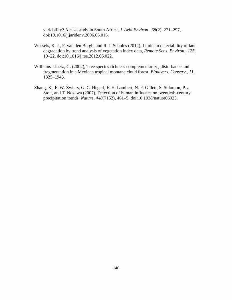
140
variability? A case study in South Africa, J. Arid Environ., 68(2), 271–297,
doi:10.1016/j.jaridenv.2006.05.015.
Wessels, K. J., F. van den Bergh, and R. J. Scholes (2012), Limits to detectability of land
degradation by trend analysis of vegetation index data, Remote Sens. Environ., 125,
10–22, doi:10.1016/j.rse.2012.06.022.
Williams-Linera, G. (2002), Tree species richness complementarity , disturbance and
fragmentation in a Mexican tropical montane cloud forest, Biodivers. Conserv., 11,
1825–1943.
Zhang, X., F. W. Zwiers, G. C. Hegerl, F. H. Lambert, N. P. Gillett, S. Solomon, P. a
Stott, and T. Nozawa (2007), Detection of human influence on twentieth-century
precipitation trends, Nature, 448(7152), 461–5, doi:10.1038/nature06025.

141
APPENDIX A
DETAILS OF THE CANONICAL CORRESPONDENCE ANALYSIS CONDUCTED
IN CHAPTER 3
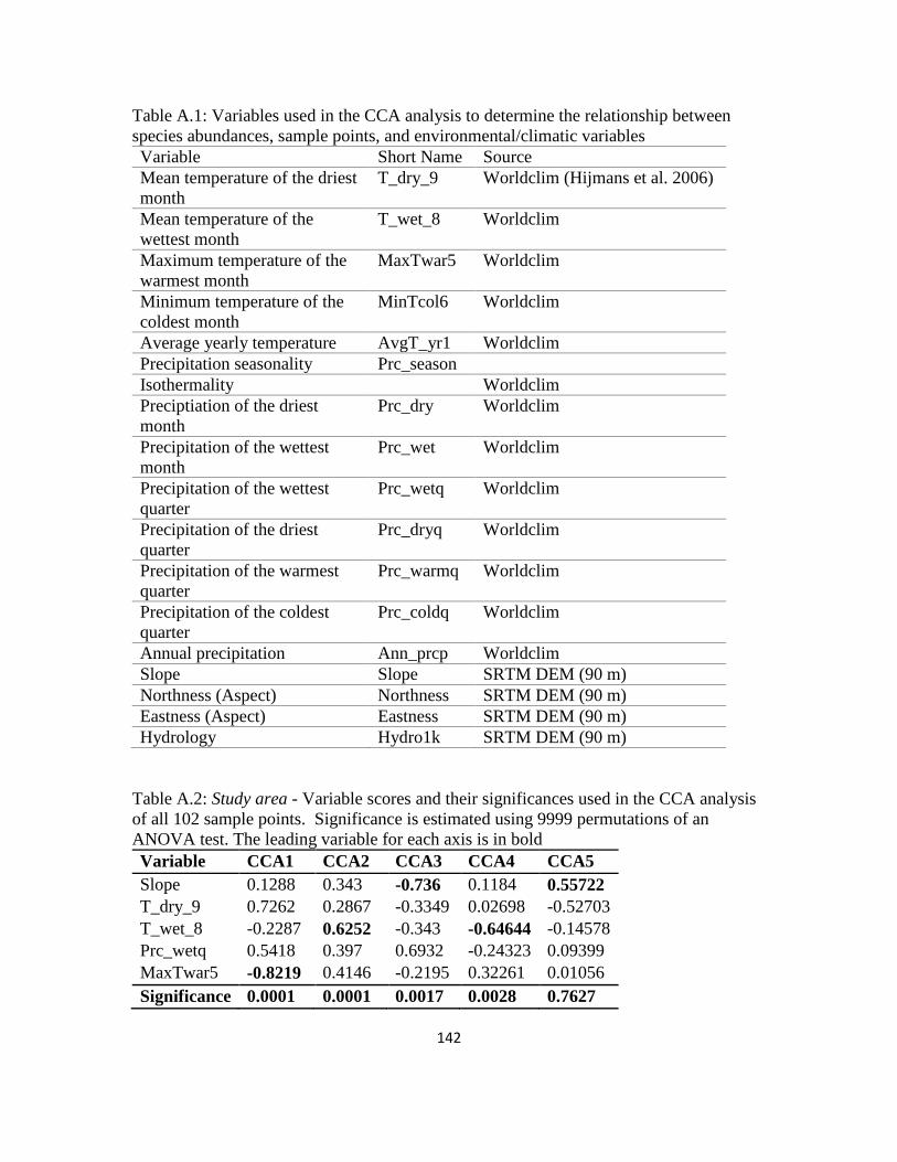
142
Table A.1: Variables used in the CCA analysis to determine the relationship between
species abundances, sample points, and environmental/climatic variables
Variable Short Name Source
Mean temperature of the driest
month
T_dry_9 Worldclim (Hijmans et al. 2006)
Mean temperature of the
wettest month
T_wet_8 Worldclim
Maximum temperature of the
warmest month
MaxTwar5 Worldclim
Minimum temperature of the
coldest month
MinTcol6 Worldclim
Average yearly temperature AvgT_yr1 Worldclim
Precipitation seasonality Prc_season
Isothermality Worldclim
Preciptiation of the driest
month
Prc_dry Worldclim
Precipitation of the wettest
month
Prc_wet Worldclim
Precipitation of the wettest
quarter
Prc_wetq Worldclim
Precipitation of the driest
quarter
Prc_dryq Worldclim
Precipitation of the warmest
quarter
Prc_warmq Worldclim
Precipitation of the coldest
quarter
Prc_coldq Worldclim
Annual precipitation Ann_prcp Worldclim
Slope Slope SRTM DEM (90 m)
Northness (Aspect) Northness SRTM DEM (90 m)
Eastness (Aspect) Eastness SRTM DEM (90 m)
Hydrology Hydro1k SRTM DEM (90 m)
Table A.2: Study area - Variable scores and their significances used in the CCA analysis
of all 102 sample points. Significance is estimated using 9999 permutations of an
ANOVA test. The leading variable for each axis is in bold
Variable CCA1 CCA2 CCA3 CCA4 CCA5
Slope 0.1288 0.343 -0.736 0.1184 0.55722
T_dry_9 0.7262 0.2867 -0.3349 0.02698 -0.52703
T_wet_8 -0.2287 0.6252 -0.343 -0.64644 -0.14578
Prc_wetq 0.5418 0.397 0.6932 -0.24323 0.09399
MaxTwar5 -0.8219 0.4146 -0.2195 0.32261 0.01056
Significance 0.0001 0.0001 0.0017 0.0028 0.7627
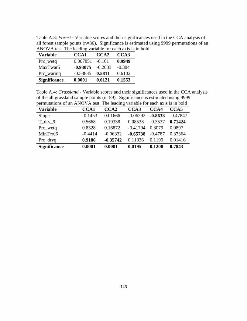
143
Table A.3: Forest - Variable scores and their significances used in the CCA analysis of
all forest sample points (n=36). Significance is estimated using 9999 permutations of an
ANOVA test. The leading variable for each axis is in bold
Variable CCA1 CCA2 CCA3
Prc_wetq 0.007851 -0.101 0.9949
MaxTwar5 -0.93075 -0.2033 -0.304
Prc_warmq -0.53835 0.5811 0.6102
Significance 0.0001 0.0121 0.1553
Table A.4: Grassland - Variable scores and their significances used in the CCA analysis
of the all grassland sample points (n=59). Significance is estimated using 9999
permutations of an ANOVA test. The leading variable for each axis is in bold
Variable CCA1 CCA2 CCA3 CCA4 CCA5
Slope -0.1453 0.01666 -0.06292 -0.8638 -0.47847
T_dry_9 0.5668 0.19338 0.08538 -0.3537 0.71424
Prc_wetq 0.8328 0.16872 -0.41794 0.3079 0.0897
MinTcol6 -0.4414 -0.06332 -0.65738 -0.4787 0.37364
Prc_dryq 0.9186 -0.35742 0.11836 0.1199 0.01416
Significance 0.0001 0.0001 0.0195 0.1208 0.7843

144
APPENDIX B
DETAILS OF THE CLUSTER ANALYSIS CONDUCTED IN CHAPTER 3
145
Figure B.1: Silhouette plot showing outliers and relative strength of the clusters identified
in the cluster analysis. The far right column contains the number of sample points in a
cluster (nj) and the silhouette width (si). si is interpreted similarly to a correlation
coefficient. Anything to the left of 0.0 is considered an outlier. The R package ‘vegan’
was used to determine the clusters and produce the figure.
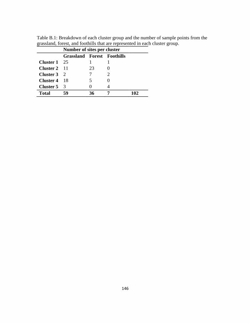
146
Table B.1: Breakdown of each cluster group and the number of sample points from the
grassland, forest, and foothills that are represented in each cluster group.
Number of sites per cluster
Grassland Forest Foothills
Cluster 1 25 1 1
Cluster 2 11 23 0
Cluster 3 2 7 2
Cluster 4 18 5 0
Cluster 5 3 0 4
Total 59 36 7 102