Understanding collective human movement dynamics during ...
22
1 Understanding collective human movement dynamics during large- scale events using big geosocial data analytics Junchuan Fan a,⁎ , Kathleen Stewart b a Oak Ridge National Laboratory, United States b Center for Geospatial Information Science, University of Maryland, College Park, United States 1. Introduction Conventional approaches for modeling human movement dynamics often focus on activity and mobility patterns in individuals’ regular daily lives (González, Hidalgo, and Barabási 2008; C. Song et al. 2010). When there are large-scale external events, traditional models may fall short in capturing changes in human movement dynamics in response to large-scale events such as earthquakes (Lu, Bengtsson, and Holme 2012; Bagrow, Wang, and Barabási 2011; X. Song et al. 2017), hurricanes (Wang and Taylor 2014; Roy, Cebrian, and Hasan 2019), epidemic outbreaks (Balcan et al. 2009; Eubank et al. 2004), and major sporting event (Marques-Neto et al. 2018). While it is critically important to understand the impact of large-scale external events on collective movement dynamics, especially for application domains such as forecasting transportation demand and emergency response, the lack of large-scale mobility data during a large-scale event poses significant challenges for researchers. With the rapid advancement of information and communication technologies, many researchers have adopted alternative data sources (e.g., cell phone records, GPS trajectory data) from private data vendors to study human movement dynamics in response to large-scale natural or societal events. With the ubiquity of location-aware mobile devices, big geosocial data, i.e., socially sensed data with georeferenced information, actively contributed by massive numbers of human sensors have also become a valuable data source for large-scale studies of human behavior (Ruths and Pfeffer 2014). Compared with other mobile device data sources such as cell phone records and GPS logs, geosocial data such as georeferenced tweets have their unique characteristics. On the one hand, they are publicly available and dynamically evolving as real-world events are happening, and users’ proactive contributions make geosocial data more likely to capture the real-time sentiments and responses of populations. On the other hand, precisely-geolocated geosocial data is scarce and biased toward urban population centers due to people’s privacy concerns and population distribution (Johnson et al. 2016). Proper data augmentation and analytic methods have
Transcript of Understanding collective human movement dynamics during ...
1
Understanding collective human movement dynamics during large-scale events using big geosocial data analytics
JunchuanFana,⁎,KathleenStewartb
aOakRidgeNationalLaboratory,UnitedStatesbCenterforGeospatialInformationScience,UniversityofMaryland,CollegePark,UnitedStates 1. Introduction
Conventional approaches for modeling human movement dynamics often focus on activity and
mobility patterns in individuals’ regular daily lives (González, Hidalgo, and Barabási 2008; C.
Song et al. 2010). When there are large-scale external events, traditional models may fall short in
capturing changes in human movement dynamics in response to large-scale events such as
earthquakes (Lu, Bengtsson, and Holme 2012; Bagrow, Wang, and Barabási 2011; X. Song et al.
2017), hurricanes (Wang and Taylor 2014; Roy, Cebrian, and Hasan 2019), epidemic outbreaks
(Balcan et al. 2009; Eubank et al. 2004), and major sporting event (Marques-Neto et al. 2018).
While it is critically important to understand the impact of large-scale external events on collective
movement dynamics, especially for application domains such as forecasting transportation
demand and emergency response, the lack of large-scale mobility data during a large-scale event
poses significant challenges for researchers. With the rapid advancement of information and
communication technologies, many researchers have adopted alternative data sources (e.g., cell
phone records, GPS trajectory data) from private data vendors to study human movement
dynamics in response to large-scale natural or societal events.
With the ubiquity of location-aware mobile devices, big geosocial data, i.e., socially sensed
data with georeferenced information, actively contributed by massive numbers of human sensors
have also become a valuable data source for large-scale studies of human behavior (Ruths and
Pfeffer 2014). Compared with other mobile device data sources such as cell phone records and
GPS logs, geosocial data such as georeferenced tweets have their unique characteristics. On the
one hand, they are publicly available and dynamically evolving as real-world events are happening,
and users’ proactive contributions make geosocial data more likely to capture the real-time
sentiments and responses of populations. On the other hand, precisely-geolocated geosocial data
is scarce and biased toward urban population centers due to people’s privacy concerns and
population distribution (Johnson et al. 2016). Proper data augmentation and analytic methods have

2
to be developed to mitigate the data scarcity and sampling bias issue of georeferenced tweets in
order to mine human activity and movement dynamics.
The 2017 Great American Eclipse was a once-in-decades total solar eclipse that passed from
the Pacific to the Atlantic coasts. The total eclipse began in Oregon at 10:16 am PDT and ended
in South Carolina at 2:44pm EDT; as the total eclipse moved from the west coast to the east coast,
it was visible within a 70 miles wide path across the entire contiguous United States, referred to
as the path of totality (POT). With 12 million people living in the path of totality (POT) and about
200 million people living within a day’s drive of the POT, hundreds of thousands of people were
estimated to have travelled to the POT to watch the total eclipse. On the day of the solar eclipse
(Aug 21, 2017), many interstate highways leading to the POT experienced unprecedented traffic
congestion, lasting hours. This event also created unprecedented challenges for many locations in
the POT. For example, more than 100,000 people flocked to Madras, Oregon, a small town of
7,000 on the eclipse day, and the Oregon National Guard had to be called in to help with logistics
and crowd control1. Uncovering human movement dynamics in response to such a large-scale
event can be extremely helpful for transportation planning, city management, or even emergency
response. The wide coverage and real-time response characteristics of Twitter data make it a data
source with a unique potential for this task. For this research, we developed a big geosocial data
analytical framework for extracting human movement dynamics in response to large-scale events
from publicly available georeferenced tweets. The framework includes a two-stage data collection
module that collects data in a more targeted fashion in order to mitigate the data scarcity issue of
georeferenced tweets; in addition, a variable bandwidth kernel density estimation (VB-KDE)
module was developed to fuse georeferenced information at different spatial scales, further
augmenting the signals of human movement dynamics contained in georeferenced tweets. The
spatial scale of collected georeferenced tweets ranges from poi to country (i.e., country, admin
(i.e., state), city, neighborhood, and poi. To correct for the inherent sampling bias of georeferenced
tweets, we adjusted the number of tweets for different spatial units (e.g., county, state) by
population. Given the social nature of geosocial data, population is an important factor for the
adjustment of tweet data sample, or geosocial data generally. There could be other sensible ways
1 https://www.orlandosentinel.com/la-sci-great-american-eclipse-liveblog-it-was-so-busy-in-madras-oregon-
they-1503273850-htmlstory.html
3
to further adjust the tweet data sampling bias depending on the specific event under study. To
demonstrate the performance of the proposed analytic framework, we chose an astronomical event
that occurred nationwide across the United States, i.e., the 2017 Great American Eclipse, as an
example event and studied the human movement dynamics in response to this event. However,
this analytic framework can easily be applied to other types of large-scale events such as hurricanes
or earthquakes. Specifically, in this research, we address the following research questions: 1) To
what extent can big geosocial data capture human movement dynamics in response to a large-
scale event; 2) What methods can be used to mitigate the widely acknowledged data sampling bias
and data scarcity issues of geosocial data in order to extract human movement dynamics from big
geosocial data; and 3) How can geospatial data be fused at different spatial scales to augment the
signals of human movement dynamics?
The rest of the paper is organized as follows: section 2 discusses related work; section 3
discusses different components of the proposed big geosocial data analytic framework, including
the two-stage data collection process and the VB-KDE module; as a validation, section 4 compares
the estimation results with traffic count reports released by State Departments of Transportation
(DOT); section 5 and 6 discusses the results and presents conclusions and future work.
2. Related work Researchers traditionally uses traffic count data or household travel survey (e.g., the National
Household Travel Survey) to track population movement dynamics. Recently, as location-enabled
devices become more common, different alternative data sources have been adopted to study
human activity patterns and movement dynamics. For example, mobile phone records of millions
of users were used to analyze the population movements after the 2010 Haiti earthquake (Lu,
Bengtsson, and Holme 2012), to examine the real-time changes in communication and mobility
pattern in the vicinity of eight emergency events (Bagrow, Wang, and Barabási 2011), and to study
the spatiotemporal dynamics of movement patterns of participants of large-scale event and the
resulting dynamics in the mobile network workload (Marques-Neto et al. 2018). GPS records
collected from mobile phones have been used to predict and simulate human mobility following
natural disasters (X. Song et al. 2017). GPS trajectory data coupled with contextual information
have been used to analyze human mobility and traffic patterns (Siła-Nowicka et al. 2016; Fan et
al. 2019).

4
Most of these data sources can only be accessed with the collaboration of private data owners.
Socially sensed data, with its public availability and real-time nature, offers researchers a unique
opportunity for large-scale studies of human behavior (Ruths and Pfeffer 2014). Researchers have
used socially sensed data to study population response to important events, be it unexpected
disaster events or planned events (Guan et al. 2014; Brambilla et al. 2017). Geosocial data was
used to estimate different aspects of human mobility, such as individual movement orbits and
travel modes (Jurdak et al. 2015), the uncertainty in regular human mobility patterns (Huang and
Wong 2015), and the impact of extreme disaster events such as hurricane, earthquake on human
mobility resilience (Roy, Cebrian, and Hasan 2019). Researchers also studied the feasibility of
using large-scale Twitter data as a proxy of human mobility for modeling and predicting disease
spread (Liu et al. 2015).
Using Twitter data to study human movement dynamics often requires inferring users’ home
locations. Various approaches have been designed to determine Twitter users’ home locations
based on available information, including using self-reported location in a user’s profile (Poblete
et al. 2011; Nguyen et al. 2017), calculating the geometric median of a user’s tweet locations
(Jurgens et al. 2015), finding the region in which a user has posted the most tweets (McNeill,
Bright, and Hale 2017), or identifying the region from which a user has posted tweets at least n
days apart (Kulshrestha et al. 2012; Hecht and Stephens 2014). Since tweets with associated
geographic coordinates are not as common due to changes in how mobile devices capture and track
movements, previous research has also explored various different ways to infer the geographic
context of tweets without relying solely on geographic coordinates provided by users. For example,
researchers have tried to infer Twitter users’ geographic locations based on the locations of users’
friends (Kong, Liu, and Huang 2014; McGee, Caverlee, and Cheng 2013). Based on the idea that
users’ tweets may encode some location-specific content, Cheng et al. proposed a probabilistic
framework for estimating Twitter users’ city-level locations based on the content of users’ tweets
(Cheng, Caverlee, and Lee 2010). The performances of these algorithms, however, did not scale
to real-world conditions (Jurgens et al. 2015). Kernel density estimation is a classic approach for
estimating home range of moving entities (Van Winkle, 1975; Worton, 1987). Bandwidth selection
is an important parameter for kernel density estimation. Adaptive kernel density estimation method
can vary the bandwidth according to the density of data points, using a narrower kernel for areas

5
with high point density and broader kernel for areas with sparse data (Salgado-Ugarte & Pérez-
Hernández, 2003; Silverman, 1986). This method was applied on geotagged tweets to construct
catchment areas of retail centers (Lloyd & Cheshire, 2017). Essentially, the goal of adaptive
kernels is to better account for data uncertainty. Given the multi-scale georeferenced tweets from
a Twitter user, this research varies the kernel bandwidth according to spatial scale of the tweet
instead of density of the tweets.
3. Analytic framework for estimating human movement dynamics from big geosocial data
In this research, we developed a big geosocial data analytic framework, TweetMovementFlow,
to extract human movement dynamics in response to large-scale events from georeferenced tweets
that includes four modules (Figure 1). The first module identifies and collects socially sensed
signals in response to the event. For the solar eclipse event, eclipse tweets, i.e., tweets that include
either the keywords ‘eclipse’ or ‘totality’, were collected during the week of the solar eclipse. The
second module creates a sample of social sensors based on collected data. For the solar eclipse
event, a collection of POT eclipse watchers, that is, Twitter users who have posted eclipse tweets
(referred to as eclipse watchers) inside the POT were identified as our sample for estimating the
human movement pattern from different states to POT states, i.e., states that intersected with the
POT. The third component infers home location of sampled social sensors in order to estimate the
origin and destination of the eclipse-watching trips made by all sampled social sensors. Since the
tweets collected in the first module was only a one-week snapshot, they were too scarce to estimate
eclipse watchers’ home state. The second stage of data collection process, i.e., retrieving tweet
histories of POT eclipse watchers, was developed in the third module. POT eclipse watchers’
home states were inferred based on their tweet histories.

6
Figure 1 Analytical framework for estimating human movement pattern to different POT states
using georeferenced tweets
The fourth component estimates aggregated movement patterns after adjusting the data sampling
bias. The fourth component aggregated the number of eclipse watchers by state and adjusted the
number by state population to estimate the percent of visitors from different states. Although this
analytic framework is presented in the context of the solar eclipse event, it can easily be adapted
to other types of large-scale events.
3.1 Spatiotemporal characteristic of eclipse tweets
In the first stage of the data collection process for this study, the location filter of the Twitter
Streaming API was used to collect only the georeferenced tweets, including both place-referenced
tweets and coordinate-referenced tweets, during the week of the Great American Solar Eclipse
(18/08/2017~08/25/2017). A place-referenced tweet has a place boundary representing the
location of tweet, with five different spatial scales, namely, country, admin (i.e., state), city,
neighborhood, and poi. A coordinate-referenced tweet has a pair of geographic coordinates
representing the location of tweet. There were 13,908,147 georeferenced tweets, out of which
331,415 were eclipse tweets, posted by 241,282 eclipse watchers.
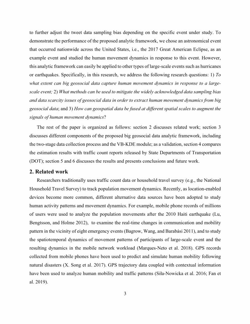
The spatial distribution of eclipse tweets collected during the eclipse week (Figure 2a) showed
that eclipse tweets were posted from all over the U.S. during the eclipse week, and urban
population centers had more coverage. Hotspot analysis was carried out for U.S. counties based
on the number of eclipse tweets in each county. Eclipse tweets with coarser than county-scale
georeferenced information were excluded from hotspot analysis (Figure 2(b) (c)). After excluding

7
eclipse tweets that were at country or state scale, there were 284,462 (85.8%) eclipse tweets with
city or finer-than-city-scale georeferenced information. The number of eclipse tweets in each U.S.
county was then counted by spatially joining place boundary center or coordinate of eclipse tweets
with U.S. counties. Figure 2b shows the result of hotspot county analysis for eclipse tweets.
Without correction for tweet data sampling bias, the hotspot counties were mostly large urban
population centers in the U.S. with high population density, reflecting tweet data’s spatial sampling
bias. After normalizing the number of eclipse tweets in each county by the county population, the
hotspot county results clearly revealed the effect of the solar eclipse event (Figure 2c). As shown
in Figure 2c, the hotspot counties for eclipse tweets were mostly counties on the POT after
adjustment by county population. The only exception was four counties in North Dakota.
Considering the noisy nature of tweet data, the hotspot county analysis results captured the eclipse
event dynamics surprisingly well. Note that the hotspot analysis results did not indicate the
absolute number of eclipse watchers in a county; rather they indicated the degree of concentration
of eclipse watchers in a county in comparison with surrounding counties. Moreover, no county
was identified as a cold spot. In other words, there was no statistically significant cluster of
counties that have a lower number of eclipse tweets than their neighboring counties. In terms of
absolute number of eclipse tweets, Tennessee had the most, followed by South Carolina and
Missouri. For eastern states that have high population density, even if a county was not in the POT,
there could still have been a large number of eclipse watchers, whereas for western states with
lower population density, counties that were not on POT had significantly fewer eclipse watchers
than POT counties. As a result, the most significant hotspot counties were POT counties from the
western states. In eastern POT states, there were two hotspot regions. The first was bordering
counties in Kentucky, Tennessee, and Illinois, including places like Nashville, TN. The second
was bordering counties of Tennessee, Georgia, North Carolina and South Carolina. This reflected
the movement choices of out-of-state eclipse watchers; and border counties were more likely to be
the destination choices for eclipse viewing.
8
Figure 2. Spatial distribution of eclipse tweets. (a) spatial distribution of eclipse tweets in the
United States; (b) hotspot counties for eclipse tweets; (c) hotspot counties for eclipse tweets after
normalizing the number of eclipse tweets by county population
The hourly temporal distribution of eclipse tweets inside and outside the POT from Aug 20th
to Aug 23rd is shown in Figure 3. The time of day information for each eclipse tweet was converted
to local time zone based on the location of the eclipse tweet. The hourly distribution of eclipse
tweets showed that the vast majority of eclipse tweets were posted on the eclipse day, Aug 21,
proving that most of the eclipse tweets were truly in-situ sensed data. Inside the POT, the peak
hour of eclipse tweets occurred at the 13th hour, which was when the totality started in the Central

9
Time Zone and where the Tennessee hotspot counties were. Interestingly, outside of the POT,
there was a small peak at the 10th hour, when the totality first started on the west coast; and the
peak hour of eclipse tweets there occurred at the 14th hour when the totality started in all the
Eastern states.
Figure 3. Hourly fluctuation of eclipse tweets inside (red) and outside (blue) POT
The hourly fluctuation of eclipse tweets clearly reflected the response of the population as the
solar eclipse moved from west to east. In addition, the in-situ nature of the eclipse tweets indicated
that the location information of eclipse tweets captured the twitter user’s location while they were
watching the eclipse. If we can infer eclipse watchers’ home locations, then we would be able to
uncover the overall movement dynamics on eclipse day based on the origin and destination
information.
3.2 Retrieving tweet histories of eclipse watchers
The hotspot counties for eclipse tweets reveal that a large number of out-of-state visitors
travelled to POT states, but could not show where these out-of-state visitors were from. From a
transportation planning perspective, understanding the origins of visitors can greatly help
transportation agencies to manage congestion on different roads and predict roadways that are
more likely to be subject to severe traffic volume increases and plan accordingly. For

10
TweetMovementFlow, we used the tweet histories of eclipse watchers to infer their home states.
Compared with previous methods, using tweet histories can significantly augment the signals of
users’ historical spatial footprints. As Twitter users’ spatial footprint histories reflect their activity
spaces in real life, the region with the most frequent tweet activities was designated as a Twitter
user’s home region. The tweet histories of all the POT eclipse watchers were collected using
Twitter user timeline API2 , which permits developers to retrieve a collection of the most recent
tweets (about 3200) posted by a Twitter user. Table 1 shows some statistics of the retrieved tweet
histories, which included 110,178,814 tweets from 212,696 eclipse watchers3.
Table 1. Statistics of tweet histories of eclipse watchers
total number of collected historical tweets
number of place- referenced tweets
number of coordinate- referenced tweets
ratio of place- referenced tweets
ratio of coordinate- referenced tweets
max 3819 3245 3244 100% 100%
min 1 1 0 0.03% 0
median 3055 345 1 17% 0.06%
mean 2456 518 102 22% 5%
As shown in Table 1, about 20% (both mean and median) of tweets from the tweet histories of
eclipse watchers were place-referenced tweets. On average, only about 5% of the tweets in their
tweet histories had coordinate information. Moreover, the median ratio of coordinate-referenced
tweets (0.06%) showed that the coordinate-referenced tweets were highly skewed among different
Twitter users, and some Twitter users did not have any coordinate-referenced tweets. Therefore,
only using coordinate-referenced tweets to infer Twitter user’s origin state was not a feasible
solution as coordinate-referenced tweets were too scarce to provide enough support for reasoning.
Since the ratio of place-referenced tweets in user tweet histories was much higher than that of
coordinate-referenced tweets, a data fusion method was designed to integrate coordinate-
2 https://developer.twitter.com/en/docs/tweets/timelines/api-reference/get-statuses-user_timeline.html 3 A small portion of Twitter users didn’t authorize developers to collect their tweet histories.
11
referenced tweets with place-referenced tweets, further augmenting the spatial footprint signals of
eclipse watchers.
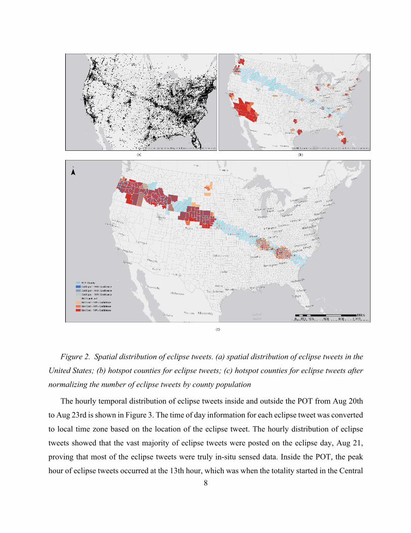
3.3 Fusing multi-scale georeference information using VB-KDE
Because the georeferenced information of place-referenced tweets can have different spatial
scales (e.g., state, city, neighborhood, poi) (Figure 4), the estimation results for different eclipse
watcher’s home region have different levels of uncertainty. Figure 4(a) and (b) show the spatial
footprint histories of two individual Twitter users; Twitter user A posted georeferenced tweets at
point, city and state scale, while Twitter user B posted only city and state-scale georeferenced
tweets.
Figure 4 (a) spatial footprint history of individual Twitter user A; (b) spatial footprint history
of individual Twitter user B; (c) spatial footprint histories of randomly sampled 10 percent of
eclipse watchers
To account for the different levels of uncertainties in the georeferenced information of tweets,
we designed a variable bandwidth kernel density estimation (VB-KDE) method. For traditional
point kernel density estimation method, bandwidth selection is an important step. For example,
ESRI’s ArcGIS calculates the bandwidth for point kernel density estimation using the following
formula:

12
𝐵𝑊! = 0.9 ∗ 𝑚𝑖𝑛(𝑆𝐷,/1
𝑙𝑛(2) ∗ 𝐷") ∗ 𝑛#$.&
This formula is based on Silverman’s rule-of-thumb bandwidth estimation formula but has been
adapted for two dimensions (Silverman 1986). SD refers to standard distance, Dm was the median
distance from all points to the mean center, and n is the number of points. If all georeferenced
tweets were coordinate-referenced, then the ArcGIS formula can be adopted to select bandwidth.
In VB-KDE, the bandwidth for georeferenced tweets varied with the scale of the georeferenced
information.𝐵𝑊!was selected to be the standard bandwidth for coordinate-referenced tweets, and
the bandwidth for place-referenced tweets was scaled according to the area of the place reference.
The specific equation is:
𝐵𝑊' = /𝐴𝑟𝑒𝑎' + 𝛼
𝛼 ∗ 𝐵𝑊!
where𝐴𝑟𝑒𝑎'was calculated from the boundary coordinates of the place reference and the unit of
𝐴𝑟𝑒𝑎'was 𝑚&. For a coordinate-referenced tweet, 𝐴𝑟𝑒𝑎'was zero, i.e.,𝐵𝑊' = 𝐵𝑊!. 𝛼was an
adjustment factor to tune the scaling effect, that was related to the spatial accuracy of point data.
For coordinate-referenced tweets, the spatial accuracy was 50~100 m; 𝛼 was set to 80 in this study.
(a) (b) (c)
Figure 5 Variable bandwidth kernel density estimation result for Twitter user A and B.
Figure 5(c) shows the VB-KDE results for two sampled Twitter users from Figure 4(a) (b). As
a comparison, Figure 5(b) also showed the KDE results using the same bandwidth, 𝐵𝑊!, for all
georeferenced tweets (place-referenced tweets were represented by the center of the place

13
boundary). As shown in Figure 5, VB-KDE results capture more of the uncertainty of coarse-scale
georeferenced data.
By applying VB-KDE on each eclipse watcher’s spatial footprint history, a probability activity
surface was generated for each eclipse watcher. By overlaying the state shapefiles with probability
activity surfaces, map algebra was used to calculate the state with the highest probabilities for each
POT eclipse watchers, which was then set to be the POT eclipse watcher’s origin state. To do a
preliminary validation of VB-KDE method, we collected the profile location information shared
by eclipse watchers and compared it with VB-KDE results. Profile location is a piece of
information voluntarily shared by Twitter users as their home location, and it can be any text. The
comparison shows the vast majority of profile locations matched our estimation results on a state
scale. Table 2 shows the top 10 most frequent profile locations for eclipse watchers from eight
POT states.
Table 2. Comparison of profile locations and VB-KDE results for eclipse watchers
Oregon Idaho Wyoming Nebraska Missouri Tennessee North Carolina
South Carolina
"Portland, OR"; "Oregon, USA"; "Portland, Oregon"; "Eugene, OR"; "Oregon"; "Corvallis, OR"; "Bend, OR"; "Salem, OR"; "Portland"; "PDX";
"Boise, ID"; "Idaho, USA"; "Boise, Idaho"; "Idaho"; "Meridian, ID"; "United States"; "Nampa, ID"; "Boise"; "Pocatello, ID"; "Idaho Falls, ID";
"Wyoming, USA"; "Laramie, WY"; "Wyoming"; "Jackson, WY"; "Casper, WY"; "Cheyenne, WY"; "Casper, Wyoming"; "Jackson Hole, Wyoming"; "United States"; "Rock Springs, Wyoming";
"Omaha, NE"; "Lincoln, NE"; "Nebraska, USA"; "Nebraska"; "Lincoln, Nebraska"; "Omaha, Nebraska"; "Omaha"; "Kearney, NE"; "Grand Island, NE"; "United States";
"Kansas City, MO"; "St Louis, MO"; "St. Louis, MO"; "Missouri, USA"; "Kansas City"; "St. Louis"; "Columbia, MO"; "Springfield, MO"; "St. Louis, Missouri"; "Missouri";
"Nashville, TN"; "Knoxville, TN"; "Memphis, TN"; "Tennessee, USA"; "Chattanooga, TN"; "Nashville"; "Tennessee"; "Murfreesboro, TN"; "Franklin, TN"; "Nashville, Tennessee";
"Charlotte, NC"; "Raleigh, NC"; "North Carolina, USA"; "North Carolina"; "Durham, NC"; "Asheville, NC"; "Greensboro, NC"; "Chapel Hill, NC"; "NC"; "Wilmington, NC";
"Charleston, SC"; "South Carolina, USA"; "Columbia, SC"; "Greenville, SC"; "South Carolina"; "Myrtle Beach, SC"; "Lexington, SC"; "United States"; "Clemson, SC"; "Columbia, South Carolina";
Without other available ground truth data, this comparison demonstrated the validity of VB-
KDE in estimating eclipse watcher’s origin state from his/her spatial footprint history.
3.4. Inflow of eclipse watchers from different states to each POT state

14
Like all sampled studies, the representativeness of a sample is critical. In the hotspot county
analysis of eclipse tweets, county population has proven to be an effective correcting factor for the
spatial sampling bias of tweets. Therefore, after estimating the origin states of POT eclipse
watchers, the number of eclipse watchers from each state were calibrated by state population,
which was used as a weighting factor, the higher the state population, the lower the weight. Then,
the weighted number of each state was divided by the weighted sum to calculate the percentage of
eclipse watchers from different states. In the following discussion, unless otherwise specified, the
number of eclipse watchers refers to the calibrated number. In total, 28,596 POT eclipse watchers
were collected as our study sample. For each POT state, the emphasis of our analysis was on the
ranked order of percent of eclipse watchers from different states rather than the absolute number
of eclipse watchers. In other words, the goal was to understand where most eclipse watchers were
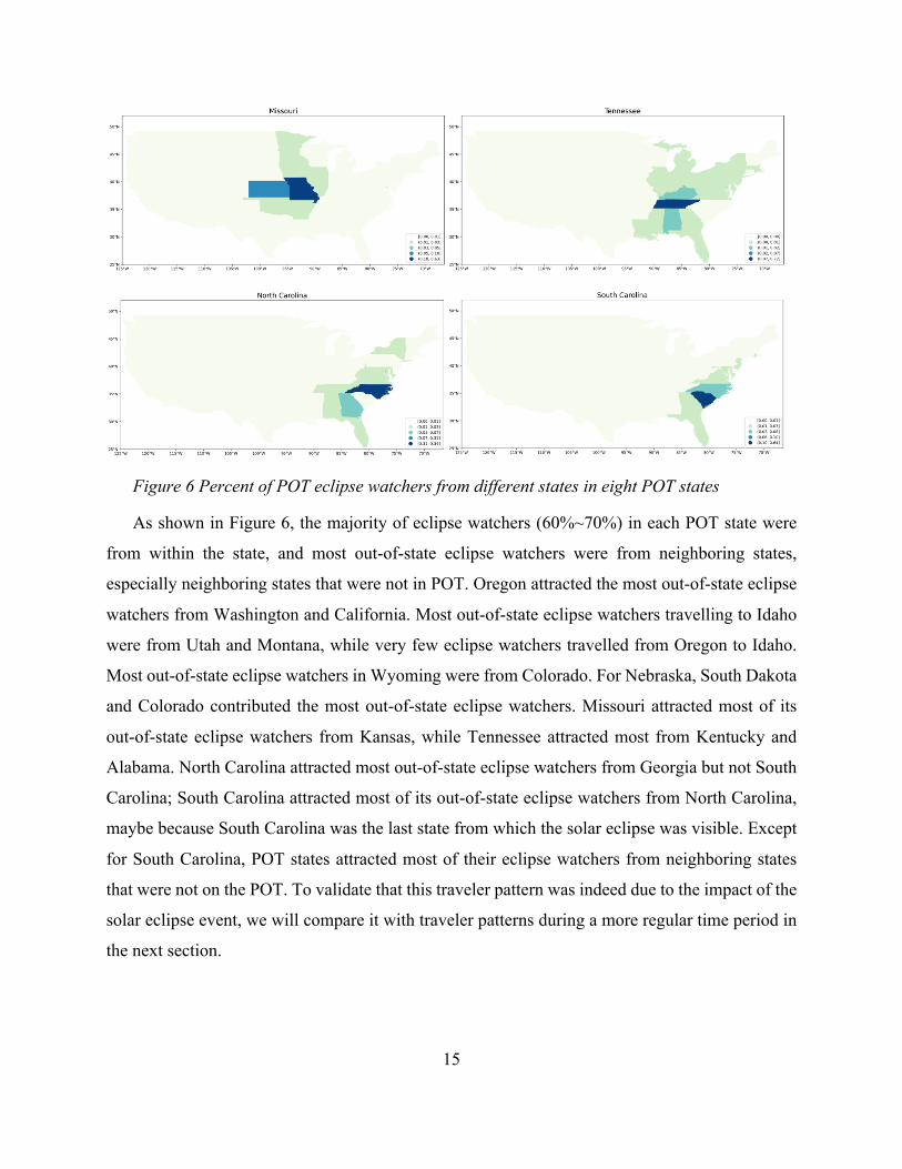
from for each POT state. Figure 6 shows the percent of eclipse watchers from different states for
each of the eight states that the POT passed through.
15
Figure 6 Percent of POT eclipse watchers from different states in eight POT states
As shown in Figure 6, the majority of eclipse watchers (60%~70%) in each POT state were
from within the state, and most out-of-state eclipse watchers were from neighboring states,
especially neighboring states that were not in POT. Oregon attracted the most out-of-state eclipse
watchers from Washington and California. Most out-of-state eclipse watchers travelling to Idaho
were from Utah and Montana, while very few eclipse watchers travelled from Oregon to Idaho.
Most out-of-state eclipse watchers in Wyoming were from Colorado. For Nebraska, South Dakota
and Colorado contributed the most out-of-state eclipse watchers. Missouri attracted most of its
out-of-state eclipse watchers from Kansas, while Tennessee attracted most from Kentucky and
Alabama. North Carolina attracted most out-of-state eclipse watchers from Georgia but not South
Carolina; South Carolina attracted most of its out-of-state eclipse watchers from North Carolina,
maybe because South Carolina was the last state from which the solar eclipse was visible. Except
for South Carolina, POT states attracted most of their eclipse watchers from neighboring states
that were not on the POT. To validate that this traveler pattern was indeed due to the impact of the
solar eclipse event, we will compare it with traveler patterns during a more regular time period in
the next section.

16
4. Results validation To validate the effectiveness of the TweetMovementFlow analytic framework, we first
compared the estimation results with the official traffic count reports released by State
Transportation agencies for two states that released their eclipse day traffic count data, namely,
Idaho and Wyoming. Our estimation results showed that the largest number of out-of-state visitors
to Idaho on the eclipse day was from Utah. This matches the Idaho State Transportation
Department’s traffic count report for eclipse day, which estimated more than 160,000 visitors came
from out of state, and the busiest road on the eclipse day was the I-15 corridor between Utah and
Idaho Falls4 (Figure 7). For Wyoming, our method estimated that most out-of-state visitors were
from Colorado, followed by Utah. This also matches with the traffic count report released by
Wyoming DOT. According to the traffic count report released by Wyoming DOT, Laramie County
located on the southeastern border between Wyoming, Colorado had the largest increase in traffic
for eclipse day and traffic on I-25 in southern Wyoming increased the most on eclipse day5. For
traffic on I-80, WYDOT reported that I-80 east of Evanston (on the border of Utah and Wyoming)
had the most significant traffic increase (Figure 7).
4 https://itd.idaho.gov/news/solar-eclipse-traffic-counts/ 5 http://www.dot.state.wy.us/news/wyoming-traffic-increased-monday-by-more-than-536000-during-aug-21-sol

17
Figure 7 Roads in Idaho and Wyoming with the highest traffic volume increase on eclipse day
To further validate that the derived movement patterns during the solar eclipse event were
indeed a reflection of population response to the event, not regular spatial interactions among
neighboring states, we selected Oregon as an example and compared the derived patterns with
patterns in a regular time period, i.e., two weeks prior to the eclipse week
(08/04/2017~08/17/2017). For this period, we identified 17,044 Twitter users who have visited
Oregon, that is, Twitter users who have tweeted in Oregon. These Twitter users were considered
as a sample of regular visitors to Oregon; over 34 million historical tweets were collected to infer
regular visitors’ home states using the VB-KDE method.

18
Figure 8 Top 10 home states for Oregon visitors during regular time and the eclipse week
As shown in Figure 8, two weeks prior to the solar eclipse event, the four neighboring states
of Oregon, Idaho, Washington, Nevada and California contributed the most visitors to Oregon. In
contrast, the ratio of visitors in Oregon that were from Idaho dropped significantly during eclipse
week, while the percent of the other three neighboring states increased the most during the eclipse
week. The change demonstrated that georeferenced tweets indeed captured human movement
dynamics in response to a large-scale event and the proposed analytic framework was able to
extract the movement pattern.
5. Sampling bias and fusion of multi-scale geosocial data Social media data, particularly geosocial data is a noisy and biased sample, but it provides a
unique perspective for researchers to explore different aspects of human dynamics. The sampling
bias of geosocial can be separated into spatial bias and temporal bias. Spatial bias is primarily
caused by the underlying population distribution, and research has demonstrated the bias towards
urban population center (Johnson et al., 2016). In this paper, we used population data as an
adjustment factor to correct the spatial sampling bias of tweet data from different states. Although
the correction effect is not perfect, population size can effectively mitigate the spatial sampling
bias largely.

19
Moreover, spatial and temporal closeness to the event is more likely to stimulate people to
provide in-situ response, as demonstrated by spatiotemporal analysis of eclipse tweets. This self-
selection process becomes almost a positive discrimination factor (Ciulla et al. 2012) for using
geosocial data to study collective human movement dynamics. In comparison with traditional data
sources, the real-time, in-situ, shallow but wide nature of geosocial data is actually well suited for
studying human dynamics in response to large-scale natural and social events. We can easily
imagine applying the proposed big geosocial data analytic framework to other scenarios such as
hurricane evacuations, disease outbreaks, where large-scale real-time data sources that have big
enough coverage are not yet available.
As we enter the era of Internet of Things, different location-aware devices (e.g., mobile phone,
GPS tracker, RFID sensor) have become ubiquitous, and spatiotemporal footprints of moving
entities will be one of the most fundamental types of data that researchers have to handle. The
fusion of spatial data from different sources and with different spatial scales will be a critical step
in the data mining process. The different scales of georeferenced information associated with
tweets is an example of data with varying scales; the proposed data fusion approach can be easily
applied to other geographic data sources.
6. Conclusions and future work In this research, we developed an analytic framework, TweetMovementFlow, to extract human
movement dynamics in response to a large-scale event from big geosocial data. Using the 2017
Great American Solar Eclipse as an example event, we demonstrated that big geosocial data could
capture the real-time response of population to large-scale events, and the proposed analytic
framework can effectively extract human movement dynamics from big geosocial data. In view
of the unique characteristics of geosocial data, we developed several approaches to mitigate the
data scarcity and sampling bias issues of geosocial data, including the two-stage data collection
process and data aggregation and calibration. We also developed a VB-KDE approach to fuse
multi-scale georeference data. Georeferenced tweets with different spatial scales have different
levels of uncertainty. VB-KDE approach can handle the changing uncertainties through varying
bandwidth. Researchers who study different aspects of human dynamics can use these approaches
to augment signals of human dynamics in socially sensed data.

20
The applicability of the proposed framework depends on the salience of an event, which is
determined by the spatiotemporal extent and semantic uniqueness of the event. The more unusual
an event is, people as social sensors are more likely to respond and tweet about it. In addition, the
population and geographic region that are more directly impacted are more likely to respond and
generate social signals about the event. These two unique characteristics of geosocial data make it
a feasible and valuable data source for studying population response to large-scale remarkable
events. Other types of large-scale events like earthquakes, hurricanes, and epidemic outbreaks have
the saliency and are also likely to stimulate a great deal of social responses from the population.
Different kinds of events will generate different changes in human movement dynamics. For
example, natural hazard like earthquake will not give the population a lot time to plan ahead;
hurricane will cause population displacement over a prolonged period of time; epidemic outbreaks
will reduce people’s mobility. The complicated changes of human movement dynamics, over
various spatial and temporal ranges, will pose significant challenges for traditional data and
analytic approaches, which further proves the value of the proposed framework. The proposed
framework could be applied to analyze these types of events by adapting the first step of the data
collection process, i.e., adjusting the spatial and temporal ranges of tweet collection, to collect
tweets about the event of interest, which should be easy to do given the semantic saliency of the
event. Other modules of the framework can be applied with minimal adaption.
For future work, several interesting topics need further study. To reduce uncertainty, we only
aggregated eclipse tweets by two spatial scales, county and state, in our analysis. However, the
majority of eclipse tweets have finer spatial scales, and we can potentially obtain human movement
dynamics with finer spatial scale. Finding a balance between spatial scale and uncertainty in
geosocial data analysis is an important topic worth further study. Moreover, solar eclipses are a
relatively unique event. In future work, we plan to apply this analytic framework to different events
for comparison.
Acknowledgement
This research has been supported in part by a grant from the Maryland Transportation Institute.
7. References
Bagrow, J. P., Wang, D., & Barabási, A.-L. (2011). Collective response of human populations to large-scale emergencies. PloS One, 6(3), e17680.

21
Balcan, D., Colizza, V., Gonçalves, B., Hu, H., Ramasco, J. J., & Vespignani, A. (2009). Multiscale mobility networks and the spatial spreading of infectious diseases. Proceedings of the National Academy of Sciences of the United States of America, 106(51), 21484–21489.
Brambilla, M., Ceri, S., Daniel, F., & Donetti, G. (2017). Spatial Analysis of Social Media Response to Live Events. In Proceedings of the 26th International Conference on World Wide Web Companion - WWW ’17 Companion. https://doi.org/10.1145/3041021.3051698
Cheng, Z., Caverlee, J., & Lee, K. (2010). You Are Where You Tweet: A Content-based Approach to Geo-locating Twitter Users. Proceedings of the 19th ACM International Conference on Information and Knowledge Management, 759–768.
Ciulla, F., Mocanu, D., Baronchelli, A., Gonçalves, B., Perra, N., & Vespignani, A. (2012). Beating the news using social media: the case study of American Idol. EPJ Data Science, 1(1), 8.
Davis, C. A., Jr., Pappa, G. L., de Oliveira, D. R. R., & de L. Arcanjo, F. (2011). Inferring the Location of Twitter Messages Based on User Relationships. Transactions in GIS, 15(6), 735–751.
Eubank, S., Guclu, H., Kumar, V. S. A., Marathe, M. V., Srinivasan, A., Toroczkai, Z., & Wang, N. (2004). Modelling disease outbreaks in realistic urban social networks. Nature, 429(6988), 180–184.
Fan, J., Fu, C., Stewart, K., & Zhang, L. (2019). Using big GPS trajectory data analytics for vehicle miles traveled estimation. Transportation Research Part C: Emerging Technologies, 103, 298–307.
González, M. C., Hidalgo, C. A., & Barabási, A.-L. (2008). Understanding individual human mobility patterns. Nature, 453(7196), 779–782.
Guan, W., Gao, H., Yang, M., Li, Y., Ma, H., Qian, W., Cao, Z., & Yang, X. (2014). Analyzing user behavior of the micro-blogging website Sina Weibo during hot social events. Physica A: Statistical Mechanics and Its Applications, 395, 340–351.
Hecht, B., & Stephens, M. (2014). A tale of cities: Urban biases in volunteered geographic information. Eighth International AAAI Conference on Weblogs and Social Media. https://www.aaai.org/ocs/index.php/ICWSM/ICWSM14/paper/viewPaper/8114
Huang, Q., & Wong, D. W. S. (2015). Modeling and Visualizing Regular Human Mobility Patterns with Uncertainty: An Example Using Twitter Data. Annals of the Association of American Geographers. Association of American Geographers, 105(6), 1179–1197.
Johnson, I. L., Sengupta, S., Schöning, J., & Hecht, B. (2016). The Geography and Importance of Localness in Geotagged Social Media. Proceedings of the 2016 CHI Conference on Human Factors in Computing Systems, 515–526.
Jurdak, R., Zhao, K., Liu, J., AbouJaoude, M., Cameron, M., & Newth, D. (2015). Understanding Human Mobility from Twitter. PloS One, 10(7), e0131469.
Jurgens, D., Finethy, T., McCorriston, J., Xu, Y. T., & Ruths, D. (2015). Geolocation prediction in twitter using social networks: A critical analysis and review of current practice. Ninth International AAAI Conference on Web and Social Media. https://www.aaai.org/ocs/index.php/ICWSM/ICWSM15/paper/viewPaper/10584
Kong, L., Liu, Z., & Huang, Y. (2014). SPOT: Locating Social Media Users Based on Social Network Context. Proceedings of the VLDB Endowment International Conference on Very Large Data Bases, 7(13), 1681–1684.
Kulshrestha, J., Kooti, F., Nikravesh, A., & Gummadi, K. P. (2012). Geographic dissection of the twitter network. Sixth International AAAI Conference on Weblogs and Social Media. https://www.aaai.org/ocs/index.php/ICWSM/ICWSM12/paper/viewPaper/4685
Liu, J., Zhao, K., Khan, S., Cameron, M., & Jurdak, R. (2015). Multi-scale population and mobility estimation with geo-tagged Tweets. 2015 31st IEEE International Conference on Data Engineering Workshops, 83–86.
Lloyd, A., & Cheshire, J. (2017). Deriving retail centre locations and catchments from geo-tagged Twitter data. Computers, Environment and Urban Systems, 61, 108–118.
Lu, X., Bengtsson, L., & Holme, P. (2012). Predictability of population displacement after the 2010 Haiti earthquake. Proceedings of the National Academy of Sciences of the United States of America,

22
109(29), 11576–11581. Marques-Neto, H. T., Xavier, F. H. Z., Xavier, W. Z., Malab, C. H. S., Ziviani, A., Silveira, L. M., &
Almeida, J. M. (2018). Understanding Human Mobility and Workload Dynamics Due to Different Large-Scale Events Using Mobile Phone Data. Journal of Network and Systems Management, 26(4), 1079–1100.
McGee, J., Caverlee, J., & Cheng, Z. (2013). Location Prediction in Social Media Based on Tie Strength. Proceedings of the 22Nd ACM International Conference on Information & Knowledge Management, 459–468.
McNeill, G., Bright, J., & Hale, S. A. (2017). Estimating local commuting patterns from geolocated Twitter data. EPJ Data Science, 6(1), 24.
Nguyen, Q. C., McCullough, M., Meng, H.-W., Paul, D., Li, D., Kath, S., Loomis, G., Nsoesie, E. O., Wen, M., Smith, K. R., & Li, F. (2017). Geotagged US Tweets as Predictors of County-Level Health Outcomes, 2015–2016. American Journal of Public Health, 107(11), 1776–1782.
Poblete, B., Garcia, R., Mendoza, M., & Jaimes, A. (2011). Do All Birds Tweet the Same?: Characterizing Twitter Around the World. Proceedings of the 20th ACM International Conference on Information and Knowledge Management, 1025–1030.
Roy, K. C., Cebrian, M., & Hasan, S. (2019). Quantifying human mobility resilience to extreme events using geo-located social media data. EPJ Data Science, 8(1), 1–15.
Ruths, D., & Pfeffer, J. (2014). Social media for large studies of behavior. Science, 346(6213), 1063–1064.
Salgado-Ugarte, I. H., & Pérez-Hernández, M. A. (2003). Exploring the Use of Variable Bandwidth Kernel Density Estimators. The Stata Journal, 3(2), 133–147.
Siła-Nowicka, K., Vandrol, J., Oshan, T., Long, J. A., Demšar, U., & Fotheringham, A. S. (2016). Analysis of human mobility patterns from GPS trajectories and contextual information. International Journal of Geographical Information Science: IJGIS, 30(5), 881–906.
Silverman, B. W. (1986). Density Estimation for Statistics and Data Analysis. https://doi.org/10.1007/978-1-4899-3324-9
Song, C., Qu, Z., Blumm, N., & Barabási, A.-L. (2010). Limits of predictability in human mobility. Science, 327(5968), 1018–1021.
Song, X., Zhang, Q., Sekimoto, Y., & Shibasaki, R. (2017). Prediction and simulation of human mobility following natural disasters. ACM Transactions on. https://dl.acm.org/citation.cfm?id=2970819
Van Winkle, W. (1975). Comparison of Several Probabilistic Home-Range Models. The Journal of Wildlife Management, 39(1), 118–123.
Wang, Q., & Taylor, J. E. (2014). Quantifying human mobility perturbation and resilience in Hurricane Sandy. PloS One, 9(11), e112608.
Worton, B. J. (1987). A review of models of home range for animal movement. Ecological Modelling, 38(3), 277–298.