This document is downloaded from DR-NTU, Nanyang Technological

University Library, Singapore.

Title Underdetermined convolutive blind source separation viatime-frequency masking

Author(s) Reju, Vaninirappuputhenpurayil Gopalan; Koh, SooNgee; Soon, Ing Yann

Citation

Reju, V. G., Koh, S. N., & Soon, I. Y. (2010).Underdetermined Convolutive Blind Source Separationvia Time-Frequency Masking. IEEE Transactions onAudio, Speech, and Language Processing, 18(1), 101-116.

Date 2009

URL http://hdl.handle.net/10220/7004

Rights

© 2009 IEEE. Personal use of this material is permitted.Permission from IEEE must be obtained for all otheruses, in any current or future media, includingreprinting/republishing this material for advertising orpromotional purposes, creating new collective works, forresale or redistribution to servers or lists, or reuse of anycopyrighted component of this work in other works. Thepublished version is available at: [DOI:http://dx.doi.org/10.1109/TASL.2009.2024380].

1

Underdetermined Convolutive Blind SourceSeparation via Time-Frequency Masking

V. G. Reju∗, Soo Ngee Koh, Senior Member, IEEE, and Ing Yann Soon

Abstract— In this paper we consider the problem of separationof unknown number of sources from their underdetermined con-volutive mixtures via time-frequency (TF) masking. We proposetwo algorithms, one for the estimation of the masks which are tobe applied to the mixture in the TF domain for the separationof signals in the frequency domain, and the other for solvingthe permutation problem. The algorithm for mask estimation isbased on the concept of angles in complex vector space. Unlikethe previously reported methods, the algorithm does not requireany estimation of the mixing matrix or the source positions formask estimation. The algorithm clusters the mixture samples inthe TF domain based on the Hermitian angle between the samplevector and a reference vector using the well known k-means orfuzzy c-means clustering algorithms. The membership functionsso obtained from the clustering algorithms are directly used asthe masks. The algorithm for solving the permutation problemclusters the estimated masks by using k-means clustering of smallgroups of nearby masks with overlap. The effectiveness of thealgorithm in separating the sources, including collinear sources,from their underdetermined convolutive mixtures obtained in areal room environment, is demonstrated.

Index Terms— Keywords: Blind source separation, Sparsecomponent analysis, Time-Frequency Masking.

I. INTRODUCTION

THE separation of signals from their mixtures without anyinformation about the sources or the mixing process is

called blind source separation (BSS). Independent componentanalysis is one of the techniques commonly used for theseparation of sources from their mixtures. Many algorithmshave been proposed for both instantaneous and convolutiveBSS. In the case where the number of sources is less thanor equal to the number of mixtures, methods based on in-dependent component analysis (ICA) [1], [2], [3], [4] arethe most popularly used. However, in practical situations thenumber of sources may be more than the number of mixturesand cases like this are called underdetermined BSS. Whenmixing is underdetermined, sparse component analysis (SCA)is shown to outperform ICA [5]. In SCA, sparsity of thesignals is utilized to separate the signals from their mixtures.A signal is said to be sparse if the signal amplitude iszero during most of the time period. However, in practicenatural signals such as speech are not very sparse in the timedomain. In [6], Bofill, et al. show that signals like speechare more sparse in the frequency domain than in the timedomain and hence if we transform the time domain signalinto the frequency domain, the sparsity can be utilized to

The authors are with the School of Electrical and Electronic En-gineering, Nanyang Technological University, Singapore-639798. (E-mail:reju@ntu.edu.sg; esnkoh@ntu.edu.sg; eiysoon@ntu.edu.sg Phone: +65-96261479; +65-67905429; +65-67905638. Fax:+65-67927660)

separate the signals from their mixtures. By utilizing sparsityin the TF domain, many algorithms have been proposedfor blind source separation of underdetermined instantaneousmixtures. The problem of underdetermined convolutive blindsource separation has also been addressed by many researchers[7], [8], [5], [9]. Convolutive mixing of the signals can bemathematically expressed as

xp(n) =Q∑q=1

L−1∑l=0

hpq (l) sq (n− l) (1)

where p = 1, · · · , P , q = 1, · · · , Q, P is the numberof mixtures, Q is the number of sources, N is the totalnumber of samples, L is the length of the mixing filters, x =[x1, x2, · · · , xP ]T are the P sensor outputs, T is the transposeoperator, xp = [xp(0), · · · , xp(N − 1)]T are the the mixturesamples at the pth sensor output, s = [s1, s2, · · · , sQ]T are thesources, sq = [sq(0), · · · , sq(N − 1)]T are the samples of theqth source and hpq(l), l = 0, · · · , L−1 is the impulse responsefrom the qth source position to the pth sensor. Using theconvolution-multiplication property, the mixing process can beexpressed in the TF domain as

X(k, t) = H (k)S(k, t) =Q∑q=1

Hq(k)Sq(k, t) (2)

where X(k, t) = [X1(k, t), · · · , XP (k, t)]T is a column vectorof the short time Fourier transform (STFT) [10] coefficientsof the P mixed signals in the kth frequency bin at timeframe t, S(k, t) = [S1(k, t), · · · , SQ(k, t)]T is the columnvector of the STFT coefficients of the Q source signals,Hq(k) = [H1q(k), · · · , HPq(k)]

T is the qth column vectorof the mixing matrix at the kth frequency bin, i.e., H (k) =[H1 (k) , · · · ,HQ (k)] is the mixing matrix at the kth fre-quency bin and Hpq(k) is the kth DFT coefficient of theimpulse response (or mixing filter) from the q th source tothe pth sensor. Here, it is assumed that the impulse responsesremain the same for all t. In this paper all the signals in thetime domain are represented by small letters whereas signalsin the frequency domain are represented by capital letters.

For underdetermined BSS of speech signals, the mostwidely used assumption is its disjoint orthogonality propertyin the TF domain [11]. Two speech signals s1 and s2 withsupports Ω1 and Ω2 in the TF plane are said to be TF-disjointif Ω1 ∩ Ω2 = ∅. However, in practice the signals may notbe perfectly disjoint. In [11] it is shown that for practicalpurposes an approximate disjoint orthogonality is sufficientfor the separation of speech signals from their mixtures.

2

The disjoint orthogonality property of the speech signals hasbeen successfully utilized for the generation of binary maskswhich can be applied to the mixtures in the TF domainfor the separation of the sources from their underdeterminedconvolutive mixtures [7], [8], [9], [5]. The techniques usedfor the estimation of masks in some of the recent papers arereviewed below.

The direction of arrival (DOA) information is utilized in[8] for the estimation of the binary masks. For the caseof three sources and two mixtures demonstrated in [8], theDOA θDOA(k, t) is estimated at each time-frequency point. Ahistogram is then plotted using the DOAs, θDOA(k, t), ∀t, andthe three peaks obtained from the histogram is taken as theDOAs of the three sources at that frequency. The q th signalis then extracted using the binary mask

Mq(k, t) ={

1 θDOAq − Δ ≤ θDOA(k, t) ≤ θDOAq + Δ0 otherwise

(3)i.e., Yq(k, t) = Mq(k, t)Xp(k, t), where q = 1, 2, 3; p = 1 or2 and Δ is the extraction range parameter.

In [7], a two stage algorithm for the extraction of thedominant sources from their mixtures is proposed. The mainassumption is that the total number of dominant sources isless than the number of microphones, but the number ofdominant sources plus the interfering sources can be greaterthan the number of microphones. Thus, in the first stage, thefrequency domain ICA algorithm is applied to the output ofthe microphones under the assumption that the number ofindependent components are equal to the number of micro-phones and in the second stage, time-frequency masking isused to improve the performance as the components separatedby the ICA algorithm will contain some residuals caused bythe interfering sources, when the total number of sourcesis more than the number of microphones. After solving thepermutation problem and estimating the number of sources inthe first stage, binary masks are obtained based on the anglesbetween the mixture sample vectors X(k, t) and the Fouriertransform of the estimated mixing filters H(k).

For the estimation of the binary masks, in [5], the impulseresponses of the channels (i.e., the mixing filters) are estimatedfirst. For the estimation of the mixing filters, it is assumedthat the sources are sparse in the time domain so that the timeinterval during which only one of the sources is effectivelypresent is estimated; then, for each estimated time interval thecross-correlation technique [12], [13] for the blind single inputmultiple output (SIMO) channel identification is applied. Sincethe single source intervals for the same source can exist atmany different time slots, after estimation of the mixing filters,they are clustered into Q clusters using the k-means clusteringalgorithm. The centroids of the clusters are then taken as theestimated channel parameters. Under the assumption that thesources in their TF domain are disjoint, the spatial directionvectors, v(k, t) = X(k,t)

||X(k,t)|| , of the mixture at each point in thekth frequency bin (after forcing the first entry of the spatialvector to real and positive) are clustered into Q clusters by

minimizing the criterion

v(k, t) ∈ Ci ⇔ i = arg minq

∥∥∥∥∥∥v(k, t) − Hq(k)e−j∠Hq1(k)∥∥∥Hq(k)∥∥∥

∥∥∥∥∥∥(4)

where Ci is the ith cluster and Hq(k) is the Fourier transformof the qth channel vector estimate. The samples in each clusterare then taken as the samples corresponding to one source.

The main shortcoming with the algorithm proposed in [8]is that it requires the DOA of the sources. The accurateestimation of DOA is very difficult in a reverberant envi-ronment and when the sources are very close or collinearwith the microphone array. For the algorithms in both [7] and[5], the approximate mixing parameters are to be estimatedfirst. In [7], this is done using the ICA algorithm and henceit cannot be used when the number of dominant (or therequired) sources are more than the number of microphones.The channel estimation algorithm in [5] utilizes the assumptionthat the sources are sparse enough in the time domain foreffective channel estimation.

In this paper, utilizing the concept of angles in complexvector space [14], we propose a simple algorithm for thedesign of the separation masks which are used to separatethe sources from their underdetermined convolutive mixturesunder the assumption that the sources are sufficiently disjointin the TF domain. Same as in the TF masking approach, theproposed algorithm does not have the well known scalingproblem. In addition to that, the algorithm does not requireany geometrical information about the sources or microphones.Another advantage is that well known clustering algorithmscan be directly used and the membership function obtainedfrom the clustering algorithms can be used as the mask.Also, the additional computational complexity in estimatingthe masks due to the increase in the number of microphonesis very low. In addition to the TF masking method for theseparation of the signals, we also propose an algorithm tosolve the well known permutation problem. The algorithmis based on k-means clustering, where the estimated maskswill be clustered to solve the permutation problem. Since thealready available masks are used to solve the permutationproblem, instead of using magnitude envelopes or powerratios of the separated signals, some computation time canbe saved. A similar approach for solving the permutationproblem is previously reported in [15], see Section.II-D fora brief discussion on the difference between the proposedalgorithm and that in [15]. Unlike the conventional DOA basedalgorithms [16], [17], [18], the proposed algorithms for solvingthe permutation problem does not require any geometricalinformation of the source positions and hence it can be usedeven when the sources are very close or collinear. We will alsoshow that the proposed algorithm is suitable for separation ofcollinear sources in a real room environment.

This paper is organized as follows. In the next sectionthe proposed algorithms for estimation of the masks andautomatic detection of the number of sources, followed by thealgorithm for solving the permutation problem, are described.The experimental results are given in Section III. Finally

3

Section IV concludes the paper.

II. PROPOSED METHOD

A. Basic idea

Let us first consider the case of instantaneous mixing. Forinstantaneous mixing, the impulse responses will be simplepulses of amplitude hpq , where hpq is the (p, q)th element ofthe mixing matrix. If the impulse response is a simple pulse,the imaginary part of Hpq(k) will be zero and the real part willbe the same as hpq , i.e., I{Hpq(k)} = 0 and R{Hpq(k)} =hpq , ∀k. Hence Hq(k) = hq = [h1q, · · · , hPq]T , ∀k, where hqis the qth column of the mixing matrix in the time domain andHq(k) is the qth column of the mixing matrix in the frequencydomain at the kth frequency bin. For ease of explanationassume that P = Q = 2. Now consider a point (k1, t1) in theTF plane where only the components of source s1 is present.Then from (2)

X(k1, t1) = H1(k1)S1(k1, t1) (5)

This can be written as:

R{X(k1, t1)} + jI{X(k1, t1)} =H1(k1) (R{S1(k1, t1)} + jI{S1(k1, t1)}) (6)

Since R{S1(t1, k1)} and I{S1(t1, k1)} are real, comparingreal and imaginary parts of (6), it can be seen that the directionof the column vectors R{X(k1, t1)} and I{X(k1, t1)} are thesame and it is also the same as that of H1(k1), which is thesame as that of the first column vector of the mixing matrixh1. Similarly, at another instant (k2, t2), if only source s2 ispresent, then

R{X(k2, t2)} + jI{X(k2, t2)} =H2(k2) (R{S2(k2, t2)} + jI{S2(k2, t2)}) (7)

Here the directions of both R{X(k2, t2)} and I{X(k2, t2)}are the same as that of H2(k2), which is the same as that ofthe second column vector of the mixing matrix h2. Hence ifthe sources are sparse in the TF domain, the scatter plot ofboth R{X(k, t)} and I{X(k, t)} will show a clear orientationtowards the directions of the column vectors of the mixingmatrix and once we know the directions, we can determinethe mixing matrix and hence the sources can be estimated upto a scaling factor with permutation.

When the mixing is convolutive, the column vectors H q(k)in (2) will be a complex column vector and multiplication ofthis complex vector by a complex scalar, Sq(k, t), will changethe complex-valued angle of the vectors. Hence the aboveapproach, used for instantaneous mixing, cannot be directlyapplied for convolutive mixing. Now consider two complexvectors u1 and u2. The cosine of the complex-valued anglebetween u1 and u2 is defined as [14]

cos(θC) =uH1 u2

||u1|| ||u2||(8)

where ||u|| =√

uHu and H represents the complex conjugatetranspose operation. cos(θC) in (8) can be expressed as

cos(θC) = ρejϕ (9)

where ρ ≤ 1 [14]

ρ = cos(θH) = |cos(θC)| (10)

In addition, 0 ≤ θH ≤ π/2 and −π ≤ ϕ ≤ π are called theHermitian and pseudo angle respectively between the vectorsu1 and u2 [14]. The Hermitian angle between the complexvectors u1 and u2 will remain the same even if we multiplythe vectors by any complex scalars, whereas ϕ will change (seeappendix for proof). This fact can be used for the design ofmasks for the BSS of underdetermined convolutive mixtures asfollows. Since multiplication of a complex vector by a complexscalar is not affecting the Hermitian angle between the vectorand another vector (reference vector), we take a P elementvector r, with all the elements equal to 1+ j1 as the referencevector . The Hermitian angle between the reference vector rand Hq(k) will remain the same even if we multiply Hq(k) byany complex scalar Sq(k, t). If the signals sq , q = 1, · · · , Qare sparse in the TF domain, at any point in the TF planeonly one of the source components will be present and theHermitian angle between the reference vector and the mixturevectors X(k, t) at that point will be the same as that betweenHq(k) corresponding to the source component S q(k, t) presentat that point and the reference vector r. Hence the mixturesamples in each frequency bin, k, will form Q clusters witha clear orientation with respect to the reference vector r; allthe samples in one cluster will belong to the same source.It is not necessary to make all the elements of the referencevector equal to 1+j1. In fact, any random vector can be taken.The only difference is that, for different reference vectors, theHermitian angles between the reference vectors and Hq(k),q = 1, · · · , Q will be different whereas those between thecolumn vectors Hq(k), q = 1, · · · , Q will remain the same,for a particular frequency bin. By finding the clusters, we arefinding the samples which belong to the sources correspondingto those particular clusters. In the following section this idea isillustrated with two sources and two sensors, i.e., P = Q = 2.

Assume that at point (k1, t1) only the contribution of sources1 is present, i.e., S1(k1, t1) = 0 and S2(k1, t1) = 0. Let thereference vector be r = [1 + j1, 1 + j1]T . At pont (k1, t1)the Hermitian angle Θ(k1)

H (t1) between the reference vector rand the mixture vector X(k1, t1) = [X1(k1, t1), X2(k1, t1)]T

will be the same as that between r and H1(k1, t1) =[H11(k1), H21(k1)]T . This angle, Θ(k1)

H (t1), will be the samefor all the points in the frequency bin k1, where only thecomponent of the source s1 is present. Similarly at anotherpoint, (k1, t2), if S1(k1, t2) = 0 and S2(k1, t2) = 0, theHermitian angle Θ(k1)

H (t2) between r and X(k1, t2) will be thesame as that between r and H2(k1) = [H12(k1), H22(k1)]T

and this will remain the same for all the points in thefrequency bin k1 where only the component of source s2 ispresent. Hence if we calculate the Hermitian angle between rand X(k1, t), ∀t, depending on presence or absence of thecomponents of the sources, there will be a clear groupingof the mixture vectors according to the Hermitian anglesbetween the reference vector and the mixture vectors. This isdemonstrated in Fig.1(a) where the Hermitian angle betweenthe reference vector r and H1(k) is 14.96o and that between r

4

and H2(k) is 29.40o for k = 54. In practice the signals in theTF domain may not be fully sparse, i.e., there may be instantswhere both the components of sources s1 and s2 are present.However, as demonstrated in [11] for the case of instantaneousmixing, for speech signals, approximate sparsity or disjointorthogonality is sufficient for the separation of sources fromtheir mixtures via binary masking.

For a general case of P mixtures and Q sources, theHermitian angle between the reference vector r having Pelements (say each element is 1+j1), and each of the mixturevectors in the kth

1 frequency bin, X(k1, t), ∀t is calculated, toobtain a vector of Hermitian angles, Θ(k1)

H , where the valueof Θ(k1)

H at t1 is given by

Θ(k1)H (t1) = cos−1 (|cos(θC(k1, t1))|) (11)

cos(θC(k1, t1)) =X(k1, t1)Hr

||X(k1, t1)|| ||r||(12)

The Hermitian angle vector, Θ(k)H , calculated for the frequency

bin k is used for partitioning the mixture samples in the k th

frequency bin. The membership functions for the partitioningof the samples so obtained from the clustering algorithm areused as the mask, Mq(k, t), ∀t, which will be multiplied by themixture in the TF domain,Xp(k, t), ∀t, to obtain the separatedsignal Yq(k, t), ∀t in the TF domain, i.e.,

Yq(k, t) = Mq(k, t)Xp(k, t), ∀t, q = 1, · · · , Q (13)

where p ∈ {1, · · · , P} is the index of the microphone outputto which the mask is applied.

B. Clustering of mixture samples and mask estimation

The partitioning of the values of Θ(k)H and hence the

corresponding mixture samples in the TF domain into differentgroups can be done using the well established data clusteringalgorithms [19], [20]. In this paper we examine the use oftwo well known clustering algorithms namely, k-means [20]and fuzzy c-means (FCM) [21] clustering algorithms for thepartitioning of samples in Θ(k)

H . The k-means algorithm is ahard partitioning technique, which means that any sample inthe data vector to be clustered will be fully assigned to any oneof the clusters, i.e., the membership function will be binary (0or 1). Hence if we use the membership function obtained fromthe k-means algorithm as the mask, it will be a binary mask.On the other hand the FCM algorithm is a soft partitioningtechnique and hence the mask generated by FCM will be asmooth one compared to that from the k-means algorithm. Inthe following section the clustering and the mask estimationprocedure using the k-means and fuzzy c-means algorithmsare explained in detail.

1) k-means clustering: If the samples in the TF domainis perfectly sparse, the vector of Hermitian angles Θ (k)

H willcontain only Q different values, each corresponding to aparticular source and hence we can partition the samplesperfectly without any ambiguity. However, in a real situationthis may not be the case. Hence we have to use a clusteringalgorithm to partition the samples into different clusters. TheHermitian angles in degree, calculated for k = 54, P = Q = 2

0 40 80 120 160 2000

14.9629.40

90

(a)

Θ(k

)H

(deg

) −−−Θ(k)H (t)

0 40 80 120 160 2000

0.5

1

(b)

Am

plitu

de

−−MKM1 (k, t)

−−−MKM2 (k, t)

0 40 80 120 160 2000

5

10

(c)

Am

plitu

de

−− |H11(k)S1(k, t)|

−−− |H12(k)S2(k, t)|

0 40 80 120 160 2000

5

10

(d)

Am

plitu

de

−− |Y1(k, t)|

−−− |Y2(k, t)|

Block index (t)

Fig. 1. Masks generated by k-means clustering algorithm for frequency bink = 54.

is shown in Fig.1(a). From the Figure, it is clear that most ofthe values are either close to 14.96o or to 29.40o, which arethe actual directions of the mixing vectors H1(k) and H2(k)respectively with respect to the reference vector r. Using thek-means algorithm we can partition the samples in Θ (k)

H into2 clusters. Since the k-means algorithm is a hard partitioningtechnique, each sample will belong to either one of the clustersand the membership function obtained will be binary ( 0 or 1).The direction of the estimated mixing matrix is the centroidof the angles corresponding to that particular cluster. Sincewe are estimating the signals by masking, our main interest ison the estimated membership function, which will be used asthe mask. The membership functions obtained from k-meansclustering are purely binary. To make it smoother, the samplesaway from the mean direction or centroid by Δφ are giventhe membership value cos(Δφ). The membership function soobtained are used as the mask, as shown in Fig.1(b), which ismultiplied with the mixture samples obtained from one of themicrophone outputs in the TF plane. Fig.1(c) is the magnitudeenvelope of the DFT coefficient of the clean signals picked upby the microphone on which the mask is applied. Fig.1(d) isthe magnitude envelope of the estimated signals obtained byapplying the mask on the mixture samples in the TF domain.

It is a well known fact that the starting centroid of the k-means clustering algorithm will have an impact on the finalcentroid of the clusters [22]. Hence in our algorithm, weinitialized the k-means algorithm with the result obtained fromthe histogram method on Θ(k)

H , i.e., the k-means algorithm isinitialized with the bin centers of the highest Q bins in thehistogram. We start with max(10, Q) bins and if any one ofthe highest Q bins are empty (this happens when the anglebetween the column vectors Hq(k), q = 1, · · · , Q are verysmall), the number of bins are doubled to reduce the binwidth and the histogram estimation is repeated. This processis repeated until none of the Q bins is empty.

2) Fuzzy c-means clustering: The k-means algorithm de-scribed in Section II-B.1 is a hard partitioning method, andas a result of which the estimated signal will contain abrupt

5

0 40 80 120 160 2000 14.9629.40

90

(a)

Θ

(k)

H(d

eg) −−−Θ(k)

H (t)

0 40 80 120 160 2000

0.5

1

(b)

Am

plitu

de

−−MFCM1 (k, t)

−−−MFCM2 (k, t)

0 40 80 120 160 2000

5

10

(c)

Am

plitu

de

−− |H11(k)S1(k, t)|

−−− |H12(k)S2(k, t)|

0 40 80 120 160 2000

5

10

(d)

Am

plitu

de

−− |Y1(k, t)|

−−− |Y2(k, t)|

Block index (t)

Fig. 2. Masks generated by FCM clustering algorithm for frequency bink = 54.

changes in their amplitude as shown in Fig.1(d). Theseabrupt changes in the amplitude will introduce artifacts inthe reconstructed signals in the time domain. To avoid thisproblem we examine the use of the FCM clustering algorithm,which partitions the samples into clusters with membershipvalues which are inversely related to the distance of Θ (k)

H (t)to the centroids of the clusters. For example, if a sampleis equidistant from the estimated centroids of the clusters,the k-means clustering algorithm will assign that sample toone of the clusters, with membership value equal to 1 withrespect to the cluster into which the sample is assigned andzero for the other clusters, i.e., the membership function willbe binary. In the case of the FCM algorithm, for the samecondition, the sample will be assigned to all the clusters withequal membership values of 1/Q, where Q is the numberof clusters. The FCM algorithm when applied to the samefrequency bin as that used in Section II-B.1 is shown is Fig.2.From the Figure it can be seen that the mask, which is thesame as the membership function obtained from the FCMalgorithm, is smooth and hence the magnitude envelope ofthe DFT coefficients of the estimated signals are also smooth.Consequently, it will reduce the artifacts in the reconstructedspeech signals in the time domain. However, as shown inSection III-A, the reduction in artifacts is at the cost ofreduction is signal to interference ratio (SIR).

C. Automatic detection of the number of sources

In the previous section, we assumed that the total number ofsources is known in advance. However, in a practical situationthis may not be the case. Hence we need to estimate thenumber of sources present in the mixture before clusteringΘ(k)H for the mask estimation, i.e, we need to estimate the

number of clusters in Θ(k)H . Many algorithms are available in

the literature for the estimation of the number of clusters [23],[24], [25], [26]. One commonly used technique is the clustervalidation technique. In this technique, we must have someknowledge about the possible maximum number of clusters.Then the data is clustered for different number of clusters,

c, c = 2, · · · , cmax , where cmax is the possible maximumnumber of clusters. The clusters so obtained for differentvalues of c are validated using the cluster validation technique[23], [24], [25] and the number of clusters in the best clusteringis taken as the actual number of clusters. In this paper weuse a recently reported cluster validation technique [24] forthe estimation of the number of clusters. Since our data areone dimensional, the validation index proposed in [24] formultidimensional data can be simplified as

Validation index V (U,Ψ, c) = Scat (c)+Sep (c)

Sep (cmax)(14)

where the different column vectors of U ∈ RT ×c contains

the membership values of the data to different clusters, Ψ =[ψ1, · · · , ψc]T , ψi is the centroid of the ith cluster, c is thetotal number of clusters, T is the total number of samples inΘ(k)H . Here Scat (c) represents the compactness of the obtained

cluster when the number of clusters is c

Scat (c) =

1c

c∑i=1

σψi

σΘ

(k)H

(15)

σΘ

(k)H

=1T

T∑t=1

(Θ(k)H (t) − Θ(k)

H

)2

(16)

σψi =1T

T∑t=1

uti

(Θ(k)H (t) − ψi

)2

(17)

Θ(k)H =

1T

T∑t=1

Θ(k)H (t) (18)

The range of Scat (c) is between 0 and 1. For compact clus-tering Scat (c) will be smaller. The term Sep (c) representsthe separation between the clusters, which is given by

Sep (c) =d2max

d2min

c∑i=1

⎛⎝ c∑j=1

(ψi − ψj)2

⎞⎠

−1

(19)

dmin = mini�=j

|ψi − ψj | (20)

anddmax = max

i�=j|ψi − ψj | (21)

The value of Sep (c) will be smaller when the cluster cen-ters are well distributed and larger for irregular cluster cen-ters. Hence the best clustering is the one which minimizesV (U,Ψ, c).

The source contribution from different sources will bedifferent in each frequency bins and in some bins the con-tribution from some of the sources may be very weak. Hencethe number of clusters (or sources) estimated from a singlefrequency bin will not be reliable. To make the estimationmore robust, the cluster validation technique is applied tomany frequency bins and the number which is most frequentlydetected over these frequency bins is taken as the actualnumber, Q, of sources present.

6

D. Permutation problem

The main weaknesses with frequency domain blind sourceseparation are the scaling and the permutation problems. Sincewe are applying the masks directly to the mixture in the TFdomain without any other stage in front of it, the well knownscaling problem is avoided. In general, this is true for allTF making approaches. We therefore only need to solve thepermutation problem. In the literature many algorithms havebeen reported for solving the permutation problems [27], [16],[17], [18], [28], [29], [30], [31]. The DOA based algorithms[16], [17], [18], [28] are not effective in highly reverberantenvironments or when the sources are collinear or very closeto one another [30]. In [27] it is shown that for speech signals,the magnitude envelopes of the adjacent frequency bin in theTF domain are highly correlated and this property can beused to solve the permutation problem. Later in [29] it isshown that the correlation between the power ratios are moresuitable than that between the magnitude envelopes. This factis further verified in Fig.3, where in Fig.3(a), the correlationmatrix whose entries are the correlations between the bin wisemagnitude envelopes of the STFT coefficients of the two cleansignals s1 and s2 picked up by the microphones are shown.In the Figure, the magnitudes of the entries in the correlationmatrix are shown by gray levels. The above correlation matrixCmag

S1S2∈ R

2K′×2K

′is calculated as:

Cmag

S1S2=

[RS1S1

RS1S2

RS2S1RS2S2

](22)

where RSiSj∈ R

K′×K′

, i, j ∈ {1, 2} is the correlation

matrix whose (m,n)th element,(RSiSj

)mn

, is the Pearson

correlation coefficient between mth and nth rows of Si ∈RK

′×T and Sj ∈ RK

′×T respectively, K′= K

2 + 1 if DFTlength K is even; otherwise K

′= K+1

2 and T is the totalnumber of samples in each frequency bin. Because of theconjugate smmetry property of the DFT coefficients, only thefirst K

′bins are taken. The (k, t)th element of Sq , q ∈ {1, 2},

is given by

Sq(k, t) =∣∣∣Sq(k, t)∣∣∣ (23)

Here, Sq(k, t) are the STFT coefficients of sq = hpq ∗ sq,which is the clean signal picked up by the pth microphone towhich the mask is applied.

The correlations between the bin wise power ratios of theSTFT coefficients of the signals are shown in Fig.3(b). Thecorrelation matrix is defined as:

CPratio

S1S2=

[RP ratio

S1P ratio

S1RP ratio

S1P ratio

S2

RP ratioS2

P ratioS1

RP ratioS2

P ratioS2

](24)

where P ratioSq

(k, t) = ||Sq(k,t)||2||S1(k,t)||2+||S2(k,t)||2 , q = 1, 2, k =

1, · · · ,K ′, ∀t and the correlation matrix RP ratio

SiP ratio

Sj

∈

RK

′×K

′, i, j ∈ {1, 2} is defined in a similar way as that

in (22). (The size of all the correlation matrices shown in

Fig.3 are the same as that of Cmag

S1S2). Comparing Fig.3(a)

and (b), it can be seen that the correlation between the powerratios is the better choice than that between the magnitudeenvelops for solving the permutation problem. The reason forthe improvement in performance are [29] as follows: 1) Thevalues of power ratios are clearly bounded between 0 and 1. 2)Because of the sparseness of the signals, most of the time, thepower ratios will be closer to either 0 or 1. 3) The power ratiosof different sources are exclusive to each other, i.e., for a twosource case, if P ratio

S1(k, t) is close to 1 then P ratio

S2(k, t) will be

close to 0. This shows that the binary mask or the membershipfunctions obtained from the clustering algorithms in Section II-B are the ideal candidates to replace the power ratios in solvingthe permutation problem as their values are also close to either1 or 0. This approach has another advantage that we neednot calculate the power ratios; instead, the already availablemasks/membership functions can be used which will savesome computation time. The correlations calculated betweenthe power ratios of the STFT coefficients in each frequency binof the separated signals, CP ratio

Y1Y2, and that between the masks,

CM1M2 , are shown respectively in Fig.3(c) and (d). (In caseswhere it is necessary to specify the algorithm used to estimatethe masks, the name of the clustering algorithm will be addedas superscript to CM1M2 and Mq. For example the correlationmatrix and the masks estimated by the k-means algorithmwill be represented as CKM

M1M2and MKM

q respectively whereasthose by the FCM algorithm will be represented as CFCM

M1M2

and MFCMq respectively). The correlation matrix CP ratio

Y1Y2is

defined similarly to CP ratio

S1S2, except that S1 and S2 are replaced

by Y1 and Y2 respectively. The correlation matrix CM1M2 iscalculated as

CM1M2 =[

RM1M1 RM1M2

RM2M1 RM2M2

](25)

where M1 ∈ RK

′×T and M2 ∈ R

K′×T are the arrays of

first K′

masks corresponding to the first and second sourcesrespectively. The correlation matrix RMiMj , i, j ∈ {1, 2} isdefined in a similar way as that in (22). For both Fig.3(c) and(d) the permutation problem is solved based on the correlationbetween the bin-wise power ratios of the separated signals andthat of the clean signals picked up by the microphone on whichthe masks are applied. From the figures it is clear that both themethods will give almost the same performance. A quantitativecomparison is given in Section III-A.

The main disadvantage of the correlation based method insolving the permutation problem is that, as the permutationin one frequency bin is solved based on the permutationof the previous frequency bins, failure in one frequency binwill lead to a complete misalignment beyond that frequencybin. Many algorithms have been proposed to circumvent thisproblem [32], [31], [30]. Sawada et al. [32] combined the DOAand correlation based approaches to improve the robustnessof the algorithm. However, the algorithm cannot be usedwhen the sources are collinear [30]. The partial separationmethod [31], [30] improved the robustness of the correlationmethod by incorporating a time domain stage in front ofthe frequency domain stage. To reduce the computationalcost, the time domain stage is normally implemented using

7

Fig. 3. Correlation matrices (a)`Cmag

S1S2

´

m′n′ , correlation between the bin-wise magnitude envelopes of the clean signals picked up by the microphones (b)`CP ratio

S1S2

´

m′n′ , correlation between the bin-wise power ratios of the clean signals picked up by the microphones (c)`CP ratio

Y1Y2

´m′n′ , Correlation between

the bin-wise power ratios of the separated signals (d)`CKM

M1M2

´m′n′ , correlation between the masks estimated using k-means clustering algorithm; in both

(c) and (d) the permutation problem is solved based on the correlation between the bin-wise power ratios of the separated signals and that of the cleansignals picked up by the microphone on which masks are applied (e)

`CKM

M1M2

´m′n′ , correlation between the masks estimated using k-means clustering

(f)`CFCM

M1M2

´m′n′ , correlation between the masks estimated using fuzzy c-means clustering; in both (e) and (f) the permutation problem is solved by the

proposed algorithm based on k-means clustering.

No. of masks assigned by k-meansFreq. algorithm to different clusters Cq ,bin q = 1, 2, · · · , 6

C1 C2 C3 C4 C5 C6

k 1 2 1 1 1 0k + 1 1 1 0 1 3 0k + 2 1 0 0 1 3 1k + 3 0 1 1 1 2 1k + 4 1 1 1 1 1 1k + 5 0 4 1 0 0 1k + 6 0 2 2 0 1 1k + 7 1 1 1 1 1 1k + 8 1 0 1 1 2 1k + 9 1 1 1 1 1 1k + 10 1 1 2 1 0 1k + 11 1 1 1 1 1 1k + 12 3 1 1 0 0 1k + 13 1 2 1 1 1 0k + 14 1 1 1 1 1 1k + 15 1 1 1 1 1 1

TABLE I

ILLUSTRATION OF MASK ASSIGNMENT TO DIFFERENT CLUSTERS

computationally efficient algorithms [33] with a small numberof unmixing filter taps so as to obtain the partially separatedsignals. The partially separated signal is then input to thefrequency domain stage where it is fully separated. Then thepermutation problem in each frequency bin is solved basedon the bin wise correlation between the magnitude envelopsof the DFT coefficients of the fully separated and partiallyseparated signals. Though we can use the partial separationmethod with an additional time domain stage in front of themasking stage, the separation of the signals using a timedomain ICA algorithm will be very poor when the mixturesare underdetermined and hence this approach could not beused. In this paper we propose an algorithm based on k-meansclustering to solve the permutation problem, where the masksare clustered into Q clusters, Cq , q = 1, · · · , Q, in such a waythat the sum of the distances Dq, q = 1, · · · , Q, is minimum.Dq is the total distance between the masks within the q th

cluster to its cluster centroid, i.e.,

minimize D =Q∑q=1

∑M

(k)i ∈Cq

i=1,··· ,Qk=kst,··· ,kend

(1 − r

M(k)i

Cq

)(26)

8

where M(k)i is the ith mask in the kth frequency bin, Cq

is the centroid of the qth cluster Cq , rM

(k)i

Cq

is the Pearson

correlation between M (k)i and the cluster centroid Cq , kst and

kend are the indices of the starting and ending frequency binsof the group of adjacent frequency bins used for clustering,i.e., the total number of frequency bins used is kend − kst +1. Here we use 1 − r

M(k)i

Cq

as the distance measure so that

masks which are highly correlated (smaller distance) will formone cluster. Since there are Q sources, we form Q clustersusing the k-means algorithm. In an ideal case, each clustermust contain one and only one mask from each frequencybin after clustering. But in practice this may not be the case,especially when the number of sources are large. Under suchsituations, we need to identify the bins in each cluster wherethe permutation could not be solved perfectly. This can bedone as follows:

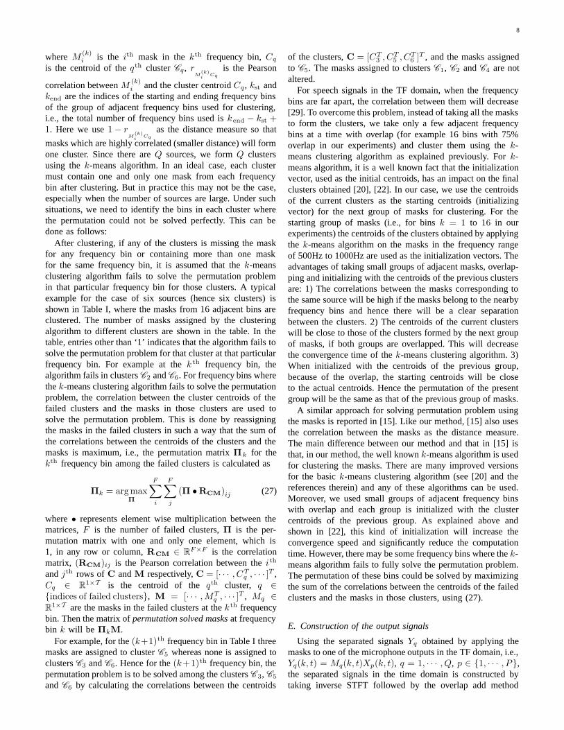
After clustering, if any of the clusters is missing the maskfor any frequency bin or containing more than one maskfor the same frequency bin, it is assumed that the k-meansclustering algorithm fails to solve the permutation problemin that particular frequency bin for those clusters. A typicalexample for the case of six sources (hence six clusters) isshown in Table I, where the masks from 16 adjacent bins areclustered. The number of masks assigned by the clusteringalgorithm to different clusters are shown in the table. In thetable, entries other than ‘1’ indicates that the algorithm fails tosolve the permutation problem for that cluster at that particularfrequency bin. For example at the k th frequency bin, thealgorithm fails in clusters C2 and C6. For frequency bins wherethe k-means clustering algorithm fails to solve the permutationproblem, the correlation between the cluster centroids of thefailed clusters and the masks in those clusters are used tosolve the permutation problem. This is done by reassigningthe masks in the failed clusters in such a way that the sum ofthe correlations between the centroids of the clusters and themasks is maximum, i.e., the permutation matrix Πk for thekth frequency bin among the failed clusters is calculated as

Πk = argmaxΠ

F∑i

F∑j

(Π •RCM)ij (27)

where • represents element wise multiplication between thematrices, F is the number of failed clusters, Π is the per-mutation matrix with one and only one element, which is1, in any row or column, RCM ∈ R

F×F is the correlationmatrix, (RCM)ij is the Pearson correlation between the ith

and jth rows of C and M respectively, C = [· · · , CTq , · · · ]T ,

Cq ∈ R1×T is the centroid of the qth cluster, q ∈

{indices of failed clusters}, M = [· · · ,MTq , · · · ]T , Mq ∈

R1×T are the masks in the failed clusters at the kth frequency

bin. Then the matrix of permutation solved masks at frequencybin k will be ΠkM.

For example, for the (k+1)th frequency bin in Table I threemasks are assigned to cluster C5 whereas none is assigned toclusters C3 and C6. Hence for the (k+1)th frequency bin, thepermutation problem is to be solved among the clusters C3, C5

and C6 by calculating the correlations between the centroids

of the clusters, C = [CT3 , CT5 , C

T6 ]T , and the masks assigned

to C5. The masks assigned to clusters C1, C2 and C4 are notaltered.

For speech signals in the TF domain, when the frequencybins are far apart, the correlation between them will decrease[29]. To overcome this problem, instead of taking all the masksto form the clusters, we take only a few adjacent frequencybins at a time with overlap (for example 16 bins with 75%overlap in our experiments) and cluster them using the k-means clustering algorithm as explained previously. For k-means algorithm, it is a well known fact that the initializationvector, used as the initial centroids, has an impact on the finalclusters obtained [20], [22]. In our case, we use the centroidsof the current clusters as the starting centroids (initializingvector) for the next group of masks for clustering. For thestarting group of masks (i.e., for bins k = 1 to 16 in ourexperiments) the centroids of the clusters obtained by applyingthe k-means algorithm on the masks in the frequency rangeof 500Hz to 1000Hz are used as the initialization vectors. Theadvantages of taking small groups of adjacent masks, overlap-ping and initializing with the centroids of the previous clustersare: 1) The correlations between the masks corresponding tothe same source will be high if the masks belong to the nearbyfrequency bins and hence there will be a clear separationbetween the clusters. 2) The centroids of the current clusterswill be close to those of the clusters formed by the next groupof masks, if both groups are overlapped. This will decreasethe convergence time of the k-means clustering algorithm. 3)When initialized with the centroids of the previous group,because of the overlap, the starting centroids will be closeto the actual centroids. Hence the permutation of the presentgroup will be the same as that of the previous group of masks.

A similar approach for solving permutation problem usingthe masks is reported in [15]. Like our method, [15] also usesthe correlation between the masks as the distance measure.The main difference between our method and that in [15] isthat, in our method, the well known k-means algorithm is usedfor clustering the masks. There are many improved versionsfor the basic k-means clustering algorithm (see [20] and thereferences therein) and any of these algorithms can be used.Moreover, we used small groups of adjacent frequency binswith overlap and each group is initialized with the clustercentroids of the previous group. As explained above andshown in [22], this kind of initialization will increase theconvergence speed and significantly reduce the computationtime. However, there may be some frequency bins where the k-means algorithm fails to fully solve the permutation problem.The permutation of these bins could be solved by maximizingthe sum of the correlations between the centroids of the failedclusters and the masks in those clusters, using (27).

E. Construction of the output signals

Using the separated signals Yq obtained by applying themasks to one of the microphone outputs in the TF domain, i.e.,Yq(k, t) = Mq(k, t)Xp(k, t), q = 1, · · · , Q, p ∈ {1, · · · , P},the separated signals in the time domain is constructed bytaking inverse STFT followed by the overlap add method

9

[10]. The masks can be applied to any one of the microphoneoutputs. However, the performance will be slightly affected bythe microphone position, please read Section.III-D for moreexplanation.

III. EXPERIMENTAL RESULTS

For performance evaluation of the proposed algorithm,both real room and simulated impulse responses are used.In Section III-A the impulse response of a real furnishedroom is used whereas for the remaining experiments, tohave a fine control on the position of the microphones andsources as well as on the acoustic environment, simulatedimpulse responses are used [34]. In all the experiments in thispaper, average performances of 50 combinations of speechutterances, selected randomly from 16 speech utterances areused. For the same number of sources, in all the experiments,the combination of speech utterances used are the same. Forexperiments in Sections III-D and III-E, the wall reflections upto 29th order is taken and humidity, temperature, absorptionof sound due to air, etc., are considered while calculatingthe impulse responses. The reverberation time, TR60, of thesimulated room is 115ms.

During the separation process, the signals may be distortedespecially when the sources are overlapped in their TF domain.Hence it is necessary to measure the distortion and the artifactsintroduced by the algorithm to assess the quality of separation.The quality of separation of the algorithm are measuredusing the method proposed in [35], [36], where the separated(estimated) signals are first decomposed into three componentsas

yq = yqtarget + eqinterf + eqartif (28)

where yqtarget is the target source with allowed deformationsuch as filtering or gain, eqinterf accounts for the interferencedue to unwanted sources and eqartif corresponds to the artifactsintroduced by the separation algorithm. Then the source todistortion ratio (SDR), source to interference ratio (SIR) andsource to artifacts ratio in dB are calculated as

SDR = 10 log10

∣∣∣∣yqtarget ∣∣∣∣2||eqinterf + eqartif ||

2 (29)

SIR = 10 log10

∣∣∣∣yqtarget ∣∣∣∣2||eqinterf ||

2 (30)

SAR = 10 log10

∣∣∣∣∣∣yqtarget+eqinterf

∣∣∣∣∣∣2||eqartif ||

2 (31)

In the proposed algorithm, since we are applying the mask toone of the microphone outputs in the TF domain, the targetsignal is taken as the signal picked up by the microphone towhich the mask is applied. Here the target source is yqtarget =hpq ∗sq where hpq is the impulse response from qth source topth microphone, if the mask is applied to the pth microphoneoutput. The other experimental conditions are: length of speechutterances are 5 seconds, speech sampling frequency is 16kHz, DFT frame size K=2048 and the window function usedis Hanning window.

Mic.1

Mic.2

s3

s1

s2

35◦

−32◦

1.33m

1.3m

1.69m

1.1m

1.4m

20cm

Room size = 4.9m×2.8m×2.65m

Microphones and sources are at 1.5m height

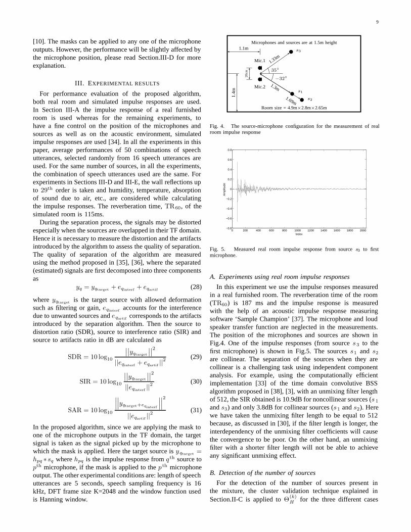
Fig. 4. The source-microphone configuration for the measurement of realroom impulse response

0 200 400 600 800 1000 1200 1400 1600 1800 2000−0.8

−0.6

−0.4

−0.2

0

0.2

0.4

0.6

0.8

Index

Am

plitu

de

Fig. 5. Measured real room impulse response from source s3 to firstmicrophone.

A. Experiments using real room impulse responses

In this experiment we use the impulse responses measuredin a real furnished room. The reverberation time of the room(TR60) is 187 ms and the impulse response is measuredwith the help of an acoustic impulse response measuringsoftware ‘Sample Champion’ [37]. The microphone and loudspeaker transfer function are neglected in the measurements.The position of the microphones and sources are shown inFig.4. One of the impulse responses (from source s3 to thefirst microphone) is shown in Fig.5. The sources s1 and s2are collinear. The separation of the sources when they arecollinear is a challenging task using independent componentanalysis. For example, using the computationally efficientimplementation [33] of the time domain convolutive BSSalgorithm proposed in [38], [3], with an unmixing filter lengthof 512, the SIR obtained is 10.9dB for noncollinear sources (s 1

and s3) and only 3.8dB for collinear sources (s1 and s2). Herewe have taken the unmixing filter length to be equal to 512because, as discussed in [30], if the filter length is longer, theinterdependency of the unmixing filter coefficients will causethe convergence to be poor. On the other hand, an unmixingfilter with a shorter filter length will not be able to achieveany significant unmixing effect.

B. Detection of the number of sources

For the detection of the number of sources present inthe mixture, the cluster validation technique explained inSection.II-C is applied to Θ(k)

H for the three different cases

10

1 2 3 4 5 60

10

20

30

40

Total number of clusters (a)

Tot

al n

o. o

f fre

q bi

ns

1 2 3 4 5 60

10

20

30

40

Total number of clusters (b)

Tot

al n

o. o

f fre

q bi

ns

1 2 3 4 5 60

10

20

30

40

50

60

Total number of clusters (c)

Tot

al n

o. o

f fre

q bi

ns0 100 200

1

2

3

4

5

6

Total no. of freq bins used (d)

Ave

rage

no.

of

cl

uste

rs e

stim

ated

0 100 2001

2

3

4

5

6

Total no. of freq bins used (e)

Ave

rage

no.

of

cl

uste

rs e

stim

ated

0 100 2001

2

3

4

5

6

Total no. of freq bins used (f)

Ave

rage

no.

of

cl

uste

rs e

stim

ated

No. of source: 2Sources: s1 and s3

No. of source: 2Sources: s1 and s2

No. of source: 2Sources: s1 and s3

No. of source: 2Sources: s1 and s2

No. of source: 3Sources: s1, s2 and s3

No. of source: 3Sources: s1, s2 and s3

Fig. 6. (a), (b) and (c) Mean histogram of the ‘estimated number of clusters (or sources)’ for the first 60 frequency bins. (d), (e) and (f) Total number offrequency bins used versus ‘estimated number of clusters (or sources) ’; the estimation result will be more reliable with higher number of frequency binsused. In the figures, at some points, the ‘number of clusters estimated’ are not integers because it is the mean performance of 50 sets of speech utterances.All the source positions are with reference to Fig.4.

shown in Fig.4. The first case involves non-collinear sources(s1 and s3), the second case collinear sources (s1 and s2)and finally the third case all the three sources (s1, s2 ands3). The mean performance obtained for 50 combinations ofspeech utterances are shown in Fig.6. Fig.6(a), (b) and (c)show the mean histogram of the estimated number of clusters(or sources) over the first 60 frequency bins for three cases ofs1 and s3, s1 and s2 and s1, s2 and s3 respectively. From theFigure it can be seen that the algorithm successfully estimatedthe number of sources in all the three cases. Fig.6(d), (e) and(f) show the total number of frequency bins used versus theestimated number of sources. The Figures clearly show thatit is not necessary to apply the cluster validation technique toall the frequency bins, instead a fraction of the total frequencybins is sufficient for the successful estimation of the numberof sources. Since the Hermitian angle calculated at any instantdepends on the relative amplitude of the source, the variationsin the calculated Hermitian angles will be high during theperiod where the unvoiced parts of the sources overlap. Forexample in Figs.1 and 2, during the period t = 80 to 120 themagnitude envelop amplitudes of the sources are small and thevariation in Hermitial angles are high. In contrast, during the

periods where the magnitude envelop amplitudes are high, thevariations in Hermitian angles are low. Considering this factin our experiments, Θ(k)

H (t) at any point where ‖X (k, t)‖ <

0.1 1T

T∑t=1

‖X (k, t)‖ are removed from Θ(k)H before clustering

them for the estimation of the number of sources. This willreduce not only the estimation error but also the computationtime. It may be noted that the samples with smaller amplitudesare removed only for the estimation of the number of clusters.For mask estimation all the samples are used.

C. Separation performance

The separation performance obtained using the proposed al-gorithm for the three cases namely collinear, non-collinear andunderdetermined with collinear sources are shown in Table II.In the Table, the performances of the algorithm when k-meansand fuzzy c-means clustering are used for the design of masksare shown for the cases where the permutation problem issolved by 1) comparing the correlation between power ratiosof the separated signals with that of the clean signals pickedup by the microphones, and 2) using the proposed k-meansclustering approach. Here the correlation between the power

11

Permutation solved using Permutation solved byActive clean signals k-means clusteringsources k-means FCM k-means FCM

Perf

orm

ance

mea

sure

Inpu

t(d

B)

Out

put

(dB

)

Impr

ovem

ent

(dB

)

Out

put

(dB

)

Impr

ovem

ent

(dB

)

Out

put

(dB

)

Impr

ovem

ent

(dB

)

Out

put

(dB

)

Impr

ovem

ent

(dB

)

s1 and s3 SDR -0.2 6.1 6.4 6.5 6.8 6.5 6.8 6.8 7.1(Non-collinear) SIR 0.0 18.2 18.2 16.8 16.8 18.9 18.9 17.3 17.3

SAR 16.1 6.6 -9.5 7.2 -8.9 6.9 -9.1 7.4 -8.6s1 and s2 SDR -0.3 4.7 5.0 5.1 5.3 5.4 5.7 5.7 5.9(Collinear) SIR -0.0 15.6 15.6 14.5 14.5 16.9 16.9 15.6 15.6

SAR 16.2 5.4 -10.8 5.9 -10.3 6.0 -10.2 6.4 -9.7s1, s2 and s3 SDR -3.4 1.8 5.2 2.0 5.4 0.5 3.9 1.0 4.4

(Underdetermined SIR -3.2 11.9 15.1 10.4 13.6 10.0 13.2 9.1 12.3with collinear) SAR 16.0 2.6 -13.4 3.2 -12.8 1.7 -14.3 2.5 -13.5

TABLE II

PERFORMANCE COMPARISON OF THE PROPOSED ALGORITHM USING k-MEANS AND FCM CLUSTERING.

Mask estimation No. of sources Time to solve the Total time to separatemethod (Each of 5 sec length) permutation problem the sources from their

alone (using the proposed mixtures.algorithm based on K-

means clustering)(seconds) (seconds)

k-means 2 2.3306 5.79113 3.2150 9.6001

FCM 2 2.2950 5.04973 3.3325 10.4966

TABLE III

ALGORITHM EXECUTION TIME

Mic

.1M

ic.2

Mic

.3M

ic.4

Mic

.5

s6

s5

s4s3

s2

s120◦

35◦

25◦30◦30◦

30◦1m

1m

1m

1m

1m

1m

2.1m1m

Room size = 4m×3m×2.5m

Microphones and sources are at 1.25m height

Fig. 7. The source-microphone configuration for the simulated room impulseresponse

ratios of the clean signals and the separated signals for solvingthe permutation problem is used as the bench mark to evaluatethe proposed k-means clustering algorithm for solving thepermutation problem because it is very robust, independentof the quality of separation in each bin and in the ideal casewhere the separation is perfect, the permutation can be solvedperfectly. The permutation matrix estimation procedure can be

mathematically expressed as follows:

Πk = argmaxΠ

Q∑i

Q∑j

(Π • RPratio

Y PratioS

)ij

(32)

where RPratioY Pratio

Sis the correlation matrix,

(RPratio

Y PratioS

)ij

is

the Pearson correlation between ith and jth rows of PratioY and

PratioS respectively, Pratio

Y is the matrix of power ratios of theseparated signals in the kth frequency bin whose tth column is

given by PratioY (t) =

[‖Y1(k,t)‖2

PQq=1 ‖Yq(k,t)‖2 , · · · ,

‖YQ(k,t)‖2

PQq=1 ‖Yq(k,t)‖2

]T.

Similarly, PratioS is the matrix of power ratios of the sig-

nal picked up by the pth microphone at the kth fre-quency bin whose column vectors are given by P ratio

S(t) =[

‖Hp1(k)S1(k,t)‖2

PQq=1 ‖HpqSq(k,t)‖2 , · · · ,

‖HpQ(k)SQ(k,t)‖2

PQq=1 ‖Hpq(k)Sq(k,t)‖2

]T, where p ∈

{1, · · · , P} is the index of the microphone to which themask is applied. From Table II, it can be seen that theSIR improvement is higher when k-means clustering is usedcompared to FCM clustering. However, the improvement inartifacts and distortion are higher when the FCM clusteringalgorithm is used. It can also be seen from the Table that theproposed method based on k-means clustering for solving thepermutation problem is as good as solving the permutationproblem by comparing the separated signals with the cleansignals. Table II show that the k-means clustering for solving

12

1 2 3 4 53

4

5

6

7

8

9

Microphone index

SD

R (

dB)

2cm5cm10cm20cm2cm5cm10cm20cm

(a)

1 2 3 4 512

13

14

15

16

17

18

19

20

21

22

Microphone index

SIR

(dB

)

2cm5cm10cm20cm2cm5cm10cm20cm

(b)

1 2 3 4 54

4.5

5

5.5

6

6.5

7

7.5

8

8.5

9

Microphone index

SA

R (

dB)

2cm5cm10cm20cm2cm5cm10cm20cm

(c)

Fig. 8. SDR/SIR/SAR versus index of the microphone output on which mask is applied, for different microphone spacings. Dotted lines are for the caseswhere the permutation problem is solved by finding the correlation between the bin-wise power ratios of the separated signals and that of clean signals pickedup by the microphones. Solid lines are for the cases where the permutation problem is solved by the proposed method based on the k-means clusteringalgorithm. The mean input SDR, SIR and SAR are -0.09dB, 0dB and 20.82dB respectively.

the permutation problem out-perform the correlation methodusing the clean signals in the experiments using two sources.The reason for this is can be explained as follows. In practice,the sources are not perfectly disjoint in their TF domain.Hence the separated signals will have some distortion whenwe use binary masking method. Due to this, the correlationbetween the separated signals or the corresponding masks inthe adjacent bins will be higher than that between the separatedsignals and the clean signals. When the number of sourcesincreases the distortion on the separated signals will be morebecause of the increased spectra overlap. If the distortions onthe separated signals are too high, the robustness of the k-means clustering algorithm will decrease and the correlationmethod using the clean signals will out-perform the k-meansclustering method.

The time taken to execute the proposed algorithm whencoded in Matlab and run in a PC with Intel Core 2 Duo 2.66GHz CPU, 2 GB of RAM is shown in Table III. Note thatthe k-means algorithm for the mask estimation is initializedwith the result obtained from the histogram method on Θ (k)

H ,whereas the FCM algorithm was initialized with randomlyselected samples from Θ(k)

H .

D. Microphone spacing and selection of microphone outputto apply mask.

The estimated mask can be applied to the mixture in theTF domain obtained from one of the microphone outputs. Inthis experiment we examine the output of the microphone onwhich the mask is to be applied to obtain the best performance.It is logical to apply the masks to the output of the centermicrophone which is proven experimentally and shown inFigs.8 to be the best choice.

In our experiments, the simulated impulse responses ob-tained for the source microphone configuration shown in Fig.7is used. Out of the total six sources, only two sources areactive at any time and hence we have a total of 6!

2!(6−2)! = 15combinations of source positions. For each combination ofsource positions the experiment is repeated for 50 sets ofutterances. The performances shown in Figs.8 are the meanperformances of these 750 experiments. To study the effect ofmicrophone spacing, these 750 experiments are repeated fordifferent microphone spacing. For this purpose microphonearrays consisting of five microphones with different spacings(2cm, 5cm, 10cm and 20cm) are used. For all the microphonespacings the center of the array is kept at the same point. The

13

2 5 10 200

5

10

15

20

25

30

35

(s1,s

2)

(s1,s

3)

(s1,s

4)

(s1,s

5)

(s1,s

6)

(s2,s

3)

(s2,s

4)

(s2,s

5)

(s2,s

6)

(s3,s

4)

(s3,s

5)

(s3,s

6)

(s4,s

5)

(s4,s

6)

(s5,s

6)

Spacing between the microphones (cm)

Δθ (

degr

ee)

Fig. 9. Variation in angle between the column vectors Hq(k), q = 1, 2versus microphone spacing. Dotted lines show the angles for different sourcecombinations, as marked in the figure, and solid line shows the mean angle.

experimental results show that the performance improves asthe spacing between the microphones increases, and after acertain distance this improvement begins to drop. The reasonfor the variation in performance because of the variation inspacing between the microphones can be explained as follows.

When the microphones are very close the difference be-tween the impulse responses of any one source and themicrophones is small. For example, the impulse responsebetween source s1 and microphone Mic.1 will be almost thesame as that between s1 and microphone Mic.2 when bothmicrophones are very close to one another. Hence in thefrequency domain, the column vectors H q(k), q = 1, · · · , Qwill be very close to one another and as a result the anglesbetween them will be small. When the angles between themixing vectors are very small, partitioning of the samples willbe difficult and the separation performance will also be poor.On the other hand, if we go on increasing the spacing, as themaximum Hermitian angle between the column vectors H q(k),q = 1, · · · , Q is π/2, after a certain distance there will not beany increase in performance. This fact is illustrated in Fig.9where the average angle between the column vectors H q(k),q = 1, · · · , Q, over the first 100 bins as a function of spacingbetween the microphones are shown.

It may be noted that, in Fig.8, for 2 cm microphone spacingthe performance is lower when the proposed k-means cluster-ing algorithm is used for solving the permutation problem thanwhen the correlation between the power ratios of the separatedand clean signals are used. This is because when the spacing issmall, the clustering of Θ(k)

H will be difficult which will leadto error in mask estimation. For the proposed algorithm forsolving the permutation problem, the robustness of the clusterformation depends on the quality of the estimated masks. Ifthe mask quality is poor, the permutation problem will notbe solved perfectly which will result in poor separation inthe time domain. When we use the correlation between theclean signals and separated signals for solving the permutationproblem, the robustness will be very high and the decrease inperformance will be mainly due to the imperfect separation ineach frequency bin, and that due to the error in solving thepermutation problem will be minimum.

E. Effect on the number of microphones

Generally in BSS, the larger the number of microphones,the better the performance. This observation also holds in ourcase. The SDR, SIR and SAR improvements for differentcombinations of number of sources and microphones areshown in Fig.10 where the masks are generated using k-means clustering. The source microphone positions are thesame as that in Fig.7. The spacings between the microphonesare fixed at 10cm for all the experiments. For the case of oddnumber of microphones, the masks are applied to the outputof the centre microphone. When the numbers of microphonesare 2 and 4, masks are applied to the first and the secondmicrophone outputs respectively. As explained in Section III-D, for two sources, because of the 15 combinations of sourceposition, 750 simulations were done. Similarly, 1000, 750,300 and 50 simulations were done for 3, 4, 5 and 6 sourcesrespectively and the mean performances so obtained are shownin Fig.10. From Figs.8 and 10, it can be seen that the binarymasking method for the separation of the sources from theirmixtures will introduce artifacts due to nonlinear distortions.This cannot be avoided and it will increase as the overlappingof the sources increases. To mitigate this problem, some postprocessing techniques have to be used [39].

IV. CONCLUSION

In this paper, an algorithm for separation of an unknownnumber of sources from their underdetermined convolutivemixtures via TF masking and a method for solving thepermutation problem by clustering the masks using k-meansclustering is proposed. The algorithm uses the membershipfunctions from the clustering algorithm as the masks. Theseparation performance of the algorithm is evaluated forthe two popular clustering algorithms, namely k-means andfuzzy c-means. The crisp nature of the membership functionsgenerated by the k-means algorithm resulted in more artifactsin the separated signals compared to those by fuzzy c-meansalgorithm, which is a soft partitioning technique. For theautomatic detection of the number of sources, the optimumnumber of clusters formed by the Hermitian angles in differentfrequency bins are estimated and the number that estimatedmost frequently is taken as the number of sources present inthe mixture. In this paper, the cluster validation technique isused for the estimation of the number of cluster; however,other techniques can also be used. In TF masking methodsfor BSS, in general, the scaling problem does not exist andthis is true for the proposed algorithm also. However, thewell-known permutation problem still exists but could besolved by clustering. The validity of the proposed algorithmsare demonstrated for both real room and simulated speechmixtures.

For the experiments in this paper, the signals used werenot sparse in the time domain. Furthermore, in the frequencydomain, the overlappings are high for larger numbers ofsources. In a practical situation, for example, conversation ina meeting room, the signals will be sparse even in the timedomain. Considering this fact and the speed of the algorithm(the algorithm will be much faster than that shown in Table III,

14

2 3 4 5

−2

0

2

4

6

8

Number of microphones(a)

Out

put S

DR

(dB

)

2 3 4 5

10

15

20

Number of microphones(b)

Out

put S

IR (

dB)

2 3 4 5

0

2

4

6

8

Number of microphones(c)

Out

put S

AR

(dB

)

2 3 4 5

5

5.5

6

6.5

7

7.5

8

8.5

Number of microphones(d)

SD

R im

prov

emen

t (dB

)

2 3 4 514

16

18

20

22

Number of microphones(e)

SIR

impr

ovem

ent (

dB)

2 3 4 5−22

−20

−18

−16

−14

−12

Number of microphones(f)

SA

R im

prov

emen

t (dB

)

2 sources 3 sources 4 sources 5 sources 6 sources

Fig. 10. Performance versus number of microphones. (a) output SDR (b) output SIR (c) output SAR (d) SDR improvement (i.e., output SDR - input SDR)(e) SIR improvement (f) SAR improvement.

if we implement it in other languages such as C or C++), theproposed algorithm is suitable for real world applications.

APPENDIX

If we multiply u1 and u2 by the complex scalars a and brespectively, then (8) will become

cos(θC) =(au1)H(bu2)√

(au1)H(au1)√

(bu2)H(bu2)

=∑

i a∗u∗i1bui2√∑

i a∗u∗i1aui1

√∑i b

∗u∗i2bui2

(33)

where uiq is the ith element of the column vector uq and *represents the complex conjugate operation. Let

a = AejθA (34)

b = BejθB (35)

ui1 = Ui1ejφi (36)

ui2 = Ui2ejψi (37)

then cos(θC) will be as shown in (39) and

cos(θH) = |cos(θC)|

=

∣∣ej(θB−θA)∑i Ui1Ui2e

j(ψi−φi)∣∣√∑

i U2i1

√∑i U

2i2

=

∣∣ej(θB−θA)∣∣ ∣∣∑

i Ui1Ui2ej(ψi−φi)

∣∣√∑i U

2i1

√∑i U

2i2

=

∣∣∑i Ui1Ui2e

j(ψi−φi)∣∣√∑

i U2i1

√∑i U

2i2

(38)

which is independent of a and b.

cos(θC) =∑iAe

−jθAUi1e−jφiBejθBUi2e

jψi√∑iAe

−jθAUi1e−jφiAejθAUi1ejφi

√∑iBe

−jθBUi2e−jψiBejθBUi2ejψi

=ABej(θB−θA)

∑i Ui1Ui2e

j(ψi−φi)

A√∑

i U2i1B

√∑i U

2i2

=ej(θB−θA)

∑i Ui1Ui2e

j(ψi−φi)√∑i U

2i1

√∑i U

2i2

(39)

15

REFERENCES

[1] A. Hyvrinen, J. Karhunen, and E. Oja, Independent Component Analysis.John Wiley & Sons Ltd, New York, 2001.

[2] A. Cichocki and S. Amari, Adaptive Blind Signal and Image Processing.John Wiley & Sons Ltd, New York, 2002.

[3] H.Buchner, R. Aichner, and W. Kellermann, “A generalization of blindsource separation algorithms for convolutive mixtures based on second-order statistics,” IEEE Transactions on Speech and Audio Processing,vol. 13, pp. 120–134, Jan. 2005.

[4] S. C. Douglas, M. Gupta, H. Sawada, and S. Makino, “Spatio-TemporalFastICA algorithms for the blind separation of convolutive mixtures,”IEEE Transactions on Audio, Speech and Language Processing, vol. 15,pp. 1511–1520, July 2007.

[5] A. Aissa-El-Bey, K. Abed-Meraim, and Y. Grenier, “Blind separationof underdetermined convolutive mixtures using their time-frequencyrepresentation,” IEEE Transactions on Audio, Speech and LanguageProcessing, vol. 15, pp. 1540–1550, July 2007.

[6] P. Bofill and M. Zibulevsky, “Underdetermined blind source separationusing sparse representation,” Signal Processing, vol. 81, pp. 2353–2362,Nov. 2001.

[7] H. Sawada, S. Araki, R. Mukai, and S. Makino, “Blind extractionof dominant target sources using ICA and Time-Frequency masking,”IEEE Transactions on Audio, Speech and Language Processing, vol. 14,pp. 2165–2173, Nov. 2006.

[8] S. Araki, S. Makino, A. Blin, R. Mukai, and H. Sawada, “Underdeter-mined blind separation for speech in real environments with sparsenessand ICA,” in Proceedings of the ICASSP, pp. iii–881–884, May 2004.

[9] S. Araki, H. Sawada, R. Mukai, and S. Makino, “Underdetermined blindsparse source separation for arbitrarily arranged multiple sensors,” SignalProcessing, vol. 87, pp. 1833–1847, Aug. 2007.

[10] A. V. Oppenheim, R. W. Schafer, and J. R. Buck, Discrete–Time SignalProcessing. Prentice Hall, 2003.

[11] O. Yilmaz and S. Rickard, “Blind separation of speech mixtures viatime–frequency masking,” IEEE Transactions on Signal Processing,vol. 52, pp. 1830–1847, July 2004.

[12] G. Xu, H. Liu, L. Tong, and T. Kailath, “A least-squares approach toblind channel identification,” IEEE Transactions on Signal Processing,vol. 43, pp. 2982–2993, Dec. 1995.

[13] A. Aissa-El-Bey, M. Grebici, K. Abed-Meraim, and A. Belouchrani,“Blind system identification using cross-relation methods: Further resultsand developments,” in Proceedings of the Int. Symp. Signal Process.Applicat., pp. 649–652, July 2003.

[14] K. Scharnhorst, “Angles in complex vector spaces,” Acta ApplicandaeMathematicae, vol. 69, pp. 95–103, Nov. 2001.

[15] H. Sawada, S. Araki, and S. Makino, “A two–stage frequency–domainblind source separation method for underdetermined convolutive mix-tures,” in Proceedings of the IEEE Workshop on Applications of SignalProcessing to Audio and Acoustics, pp. 139–142, Oct. 2007.

[16] S. Kurita, H. Saruwatari, S. Kajita, K. Takeda, and F. Itakura, “Evalu-ation of blind signal separation method using directivity pattern underreverberant conditions,” in Proceedings of the ICASSP, pp. 3140–3143,2000.

[17] H. Saruwatari, S. Kurita, K. Takeda, F. Itakura, T. Nishikawa, andK. Shikano, “Blind source separation combining independent compo-nent analysis and beamforming,” EURASIP Journal on Applied SignalProcessing, vol. 2003, no. 11, pp. 1135–1146, 2003.

[18] M. Ikram and D. Morgan, “A beamforming approach to permutationalignment for multichannel frequency domain blind speech separation,”in Proceedings of the ICASSP, pp. 881–884, 2002.

[19] A. K. Jain, M. N. Murty, and P. J. Flynn, “Data clustering: A review,”ACM Computing Surveys, vol. 31, pp. 264–323, Sept. 1999.

[20] R. Xu and Donald II Wunsch, “Survey of clustering algorithms,” IEEETransactions on Neural Networks, vol. 16, pp. 645–678, May 2005.

[21] J. C. Bezdek, Pattern Recognition With Fuzzy Objective FunctionAlgorithms. New York: Plenum Press, 1981.

[22] D. Arthur and S. Vassilvitskii, “k–means++: The advantages of carefulseeding,” in Proceedings of the eighteenth annual ACM–SIAM sympo-sium on Discrete algorithms, pp. 1027–1035, 2007.

[23] Y. Zhang, W. Wang, X. Zhang, and Y. Li, “A cluster validity index forfuzzy clustering,” Information Sciences, vol. 178, pp. 1205–1218, Feb.2008.

[24] H. Sun, S. Wang, and Q. Jiang, “FCM–based model selection algorithmsfor determining the number of clusters,” Pattern Recognition, vol. 37,pp. 2027–2037, Oct. 2004.

[25] M. K. Pakhira, S. Bandyopadhyay, and U. Maulik, “Validity index forcrisp and fuzzy clusters,” Pattern Recognition, vol. 37, pp. 487–501,Mar. 2004.

[26] P. Guo, C. L. P. Chen, and M. R. Lyu, “Cluster number selection fora small set of samples using the bayesian Ying-Yang model,” IEEETransactions on neural networks, vol. 13, pp. 757–763, May 2002.

[27] N. Murata, S. Ikeda, and A. Ziehe, “An approach to blind source sepa-ration based on temporal structure of speech signals,” Neurocomputing,vol. 41, pp. 1–24, Oct. 2001.

[28] M. Ikram and D. Morgan, “Permutation inconsistency in blind speechseparation: Investigation and solutions,” IEEE Transactions on Audio,Speech and Language Processing, vol. 13, pp. 1–13, Jan. 2005.

[29] H. Sawada, S. Araki, and S. Makino, “Measuring dependence of bin-wise separated signals for permutation alignment in frequency-domainBSS,” in IEEE Int. Symp. on Circuits and Systems, pp. 3247–3250, May2007.

[30] V. G. Reju, S. N. Koh, and I. Y. Soon, “Partial separation methodfor solving permutation problem in frequency domain blind sourceseparation of speech signals,” Neurocomputing, vol. 71, pp. 2098–2112,June 2008.

[31] V. G. Reju, S. N. Koh, and I. Y. Soon, “A robust correlation methodfor solving permutation problem in frequency domain blind sourceseparation of speech signals,” in Proceedings of the APCCAS, pp. 1893–1896, 2006.

[32] H. Sawada, R. Mukai, S. Araki, and S. Makino, “A robust and precisemethod for solving the permutation problem of frequency domain blindsource separation,” IEEE Transactions on Speech and Audio Processing,vol. 12, pp. 530–538, Sept. 2004.

[33] R. Aichner, H. Buchner, and W. Kellermann, “Real-time convolutiveblind source separation based on a broadband approach,” in FifthInternational Symposium on Independent Component Analysis and BlindSignal Separation, pp. 840–847, 2004.

[34] http://bass-db.gforge.inria.fr/BASS-dB/?show=browse&id=filters.[35] E. Vincent, R. Gribonval, and C. Fevotte, “Performance measurement

in blind audio source separation,” IEEE Transactions on Audio, Speechand Language Processing, vol. 14, pp. 1462–1469, July 2006.

[36] C. Fevotte, R. Gribonval, and E. Vincent, “BSS EVAL toolbox userguide, IRISA technical report 1706,” tech. rep., Rennes, France, Apr.2005. http://www.irisa.fr/metiss/bss eval/.

[37] http://www.purebits.com/.[38] H. Buchner, R. Aichner, and W. Kellermann, “A generalization of a

class of blind source separation algorithms for convolutive mixtures,” inProceedings of the Int. Symp. on Independent Component Analysis andBlind Signal Separation, pp. 945–950, 2003.

[39] J. Rosca, T. Gerkmann, and D. C. Balcan, “Statistical inference ofmissing speech data in the ICA domain,” in Proceedings of the ICASSP,vol. 5, pp. 617–620, May 2006.