Bank of Canada staff working papers provide a forum for staff to publish work-in-progress research independently from the Bank’s Governing Council. This research may support or challenge prevailing policy orthodoxy. Therefore, the views expressed in this paper are solely those of the authors and may differ from official Bank of Canada views. No responsibility for them should be attributed to the Bank.

www.bank-banque-canada.ca

Staff Working Paper/Document de travail du personnel 2018-22

Uncovered Return Parity: Equity Returns and Currency Returns

by Edouard Djeutem and Geoffrey R. Dunbar

ISSN 1701-9397 © 2018 Bank of Canada

Bank of Canada Staff Working Paper 2018-22

May 2018

Uncovered Return Parity: Equity Returns and Currency Returns

by

Edouard Djeutem and Geoffrey R. Dunbar

International Economic Analysis Department Bank of Canada

Ottawa, Ontario, Canada K1A 0G9 etsaguedjeutem@bankofcanada.ca

gdunbar@bankofcanada.ca

i

Acknowledgements

We thank Yu-chin Chen, Jean-Sébastian Fontaine, Pierre Guérin, Benjamin Müller, Larry Schembri, Adrien Verdelhan, Graham Voss, Todd Walker and participants at the University of Victoria, the Four Central Bank Conference (Atlanta Fed, Bank of Canada, Cleveland Fed and Swiss National Bank, November 7–9, 2017) and the Bank of Canada's Fellowship Exchange for helpful comments and discussions. Our views do not necessarily represent those of the Bank of Canada or its employees. All errors are our own.

ii

Abstract

We propose an uncovered expected returns parity (URP) condition for the bilateral spot exchange rate. URP implies that unilateral exchange rate equations are misspecified and that equity returns also affect exchange rates. Fama regressions provide evidence that URP is statistically preferred to uncovered interest rate parity (UIP) for nominal bilateral exchange rates between the US dollar and six countries (Australia, Canada, Japan, Norway, Switzerland and the UK) at the monthly frequency. An implication of URP is that commodity price changes that affect equity returns thus affect bilateral exchange rates through the equity channel. We find evidence that the Australian, Canadian, Norwegian (post 2001) and UK (post 1992) expected exchange rates increase via the oil-equity channel as oil prices rise, whereas the Japanese and Swiss expected exchange rates decrease. Bank topics: Asset pricing; Exchange rates; International financial markets JEL codes: E43, F31, G15

Résumé

Nous proposons une condition de parité des rendements sans couverture anticipés pour les taux de change bilatéraux au comptant. Cette condition implique que les équations de taux de change unilatéral sont mal spécifiées et que les rendements des actions influent également sur les taux de change. Les régressions de Fama tendent à montrer que l’hypothèse de la parité des rendements sans couverture est statistiquement préférable à celle de la parité des taux d’intérêt sans couverture pour expliquer les taux de change bilatéraux nominaux mensuels entre le dollar américain et les monnaies de six pays (Australie, Canada, Japon, Norvège, Suisse et Royaume-Uni). Il découle de cette première hypothèse que les variations des prix des produits de base ayant un effet sur les rendements des actions devraient entraîner des fluctuations des taux de change bilatéraux par le canal des actions. Nous constatons que les taux de change anticipés pour l’Australie, le Canada, la Norvège (après 2001) et le Royaume-Uni (après 1992) augmentent en phase avec les cours du pétrole par le canal des actions du secteur pétrolier, alors qu’ils diminuent pour le Japon et la Suisse. Sujets : Évaluation des actifs; Taux de change; Marchés financiers internationaux Codes JEL : E43, F31, G15

Non-Technical Summary

In general, nominal exchange rate dynamics are difficult to relate to macroeconomicsfundamentals. For example, the uncovered interest parity puzzle suggests that high inter-est rate countries tend to have higher expected currency returns, at least in the short-run.In this paper we propose a modification of the interest parity condition. Our modificationrelaxes the assumption that investors consider an interest rate parity condition, replacingit with an expected return parity condition. Throughout this paper we focus on equity asthe additional investment asset.

We augment standard uncovered interest rate parity (UIP) regressions to include adomestic portfolio of interest rate assets and equities (which we term uncovered returnparity, URP). An implication of URP is that exchange rate changes are simultaneouslydetermined by domestic and foreign portfolios. Thus, if URP is the correct data generatingprocess for exchange rate dynamics, then unilateral exchange rate models are misspecified.We specify the expected spot exchange rate as a mixture of two URP conditions and esti-mate using both OLS and a finite mixture model (FMM) for the six countries we consider.(FMM is appropriate if there is heterogeneity in country-specific information regardingaggregate portfolios.) We find empirical evidence in favour of URP and statistically rejectthat UIP, which is nested in URP, is sufficient to characterize URP. We infer that exchangerate dynamics depend on the domestic return to capital.

The URP estimates suggest that US expected excess equity returns are significant dri-vers of exchange rate movements for all countries and that US focussed investors are,on average, responsible for roughly 70–90% of the exchange rate dynamics for Canada,Japan and the UK but 10–30% for Australia, Norway and Switzerland using our FMMspecification. The FMM estimates of the posterior mixture probabilities are, however,volatile for all the countries we examine. We find evidence that interest rate differentialsare, in general, significant explanatory variables for exchange rate dynamics, particularlyfor US investors. Finally, we note that our results suggest a smaller role for currency riskpremia in nominal currency movements for the countries we examine once exchange ratesare conditioned on the carry forward return risk.

The URP condition implies that any asset that is correlated with domestic equity returnsshould also affect currency returns through the equity channel. One potential asset class iscommodities. We construct an oil return ‘factor’ that summarizes the sensitivity of excessequity returns to commodity price movements for the six countries in our sample. Ourempirical results provide evidence that oil price movements positively affect the currenciesof Australia, Canada, Norway and the UK through the equity channel and negativelyaffect the currencies of Japan and Switzerland.

1

1 Introduction

In general, nominal exchange rate dynamics are difficult to relate to macroeconomics fundamentals. This

observation has been surprisingly robust since Meese and Rogoff (1983) first noted that exchange rate

forecasting models were unlikely to beat the random walk prediction. Nominal exchange rate dynamics

are also difficult to relate to cross-country differences in nominal interest rates. For example, the uncovered

interest parity puzzle suggests that high interest rate countries tend to have higher expected currency returns,

at least in the short run.1 One possibility, which has been explored in the literature, is that existing models

either misspecify or ignore risk. Engel (2016) notes that a risk-based explanation for the uncovered interest

parity puzzle requires that the ex-ante risk premium is time-varying and covaries with the difference in

interest rates. In this paper, we propose an alternative explanation for the interest rate parity puzzle based

on a modification of the interest parity condition.

Our modification relaxes the assumption that investors consider an interest rate parity condition, re-

placing it with an expected return parity condition. Throughout this paper we focus on equity returns as

the additional investment asset. However, this choice is largely for expositional clarity as our thesis is that

exchange rate dynamics depend on a portfolio of investment returns.2 The foreign exchange market is a

decentralized exchange market with many investors who, we argue, have idiosyncratic portfolio demands.3

In the Fama regressions we consider, we augment standard uncovered interest rate parity (UIP) regressions

to include a domestic portfolio of interest assets and equities (which we term uncovered return parity, URP).

We present empirical evidence in favour of URP and statistically reject that UIP, which is nested in URP,

is sufficient to characterize URP. We infer that exchange rate dynamics depend on the domestic return to

capital.

URP has several implications for spot exchange rate markets. One is that domestic equity returns

provide an additional source of exchange rate risk. In a typical UIP environment with risk-neutral investors

(and ignoring Jensen’s inequality), there is no additional information gained from considering the foreign

perspective since the UIP condition is indifferent to the definition of the home country. The same is not

true for URP. A second implication of URP is that exchange rate changes are simultaneously determined by

domestic and foreign portfolios. If URP is the correct data-generating process for exchange rate dynamics

then unilateral exchange rate models are misspecified.

We specify the expected spot exchange rate as a mixture of two URP conditions. We estimate using

1See for example, Bilson (1981), Fama (1984), Engel (1996) and Engel (2014) for a discussion and review of the empiricalliterature.

2Thus, an alternative specification of our model could include excess returns to corporate bonds in addition to, or insteadof, equity.

3We are agnostic about the source of the differences in expectations and posit that several commonly used models such asmean-variance utility, borrowing constraints, consumption demand shocks or information asymmetry would yield such portfolios.In the Appendix, we sketch a simple model with information asymmetry that yields an aggregate portfolio composed of twodomestic assets.

2

both OLS and a finite mixture model (FMM) for the six countries we consider. FMM is appropriate if

there is heterogeneity in country-specific information regarding aggregate portfolios. If UIP is statistically

preferred to URP, then the additional URP equation should have no additional information for exchange

rate dynamics. One challenge for the empirical analysis is measuring expected equity returns. We follow

two approaches. Our first approach uses the ex post realized return and controls for potentially spurious

correlation by including contemporaneous measures of uncertainty, inflation rates and changes in equity

book-to-market. Our second approach uses the three-pass regression filter proposed by Kelly and Pruitt

(2013), Kelly and Pruitt (2015) and Guerin, Leiva-Leon, and Marcellino (2016) to extract an expected

aggregate equity return factor from publicly listed stocks on country stock exchanges. We show, using the

AIC and BIC, that the results support URP over UIP in this regression framework and FMM over OLS.

The URP condition implies that any asset that is correlated with domestic equity returns should also

affect currency returns through the equity channel. One potential asset class is commodities. Kilian and

Park (2009) and Ready (2017) argue that oil prices affect equity returns, so if the URP channel we identify is

correct, then oil prices should affect exchange rates through this channel. We construct an oil return ‘factor’

again using the three-pass regression filter proposed by Kelly and Pruitt (2013), Kelly and Pruitt (2015) and

Guerin, Leiva-Leon, and Marcellino (2016). Our empirical results provide evidence that oil price movements

positively affect the currencies of Australia, Canada, Norway and the UK through the equity channel and

negatively affect the currencies of Japan and Switzerland.

We find evidence that expected excess equity returns are significant for all countries and that US focussed

investors are, on average, responsible for roughly 70–90% of the exchange rate dynamics for Canada, Japan

and the UK but 10–30% for Australia, Norway and Switzerland using our FMM specification. The FMM

estimates of the posterior mixture probabilities are, however, volatile for all the countries we examine. One

interpretation is that the volatility is indicative of high asset mobility between these countries, at least for

some asset classes. We find evidence that interest rate differentials are, in general, significant explanatory

variables for exchange rate dynamics, particularly for US focussed investors. Finally, we note that our results

suggest a smaller role for currency risk premia in nominal currency movements for the countries we examine

once exchange rates are conditioned on the carry forward return risk.

The remainder of the paper is structured as follows. The next section presents the related literature.

Section 3 presents our parsimonious framework. Section 4 reports the data. Section 5 discusses our empirical

findings designed to test our parsimonious model and study the implications for commodities currencies.

Finally, section 6 concludes.

2 Related Literature

Our paper is related to four strands of literature.

3

The first strand investigates the financial determinants of exchange rates; see for instance Lustig and

Verdelhan (2007). This literature seeks to understand the driving forces of a cross-section of currency

excess returns using portfolio analysis common in the empirical asset pricing literature. This methodology

is also helpful in studying currency return predictability. Lu and Jacobsen (2016) argue that equity returns

predict the short leg profits of carry trades, while commodity price changes predict the long leg profits.

Passari (2017) builds an investment strategy exploiting the fact that commodity prices forecast exchange

rates at daily frequency. This strategy takes a long position in currencies that are expected to appreciate

conditional on commodity prices. The data employed in that paper cover the period January 2000 to

November 2011, which coincides with the known sharp increases in investments in currency and commodity

markets. Cenedese, Payne, Sarno, and Valente (2016) investigate the relationship between equity return

differentials and currency returns. They show that a strategy that invests in a country with high expected

equity returns and shorts countries with low expected equity returns generates excess returns. However,

their analysis concludes that the exchange rate appears to be unrelated to equity return differentials. There

are two key differences between this literature and our paper. First, we focus instead on country-specific

equity market returns. If exchange rates react asymmetrically to country-specific equity market returns,

then this is not well captured by an equity return differential. Second, our focus is to understand how the

portfolio compositions of domestic assets relate to exchange rates. We also focus on monthly returns as this

horizon is typically difficult for empirical models of UIP.

Secondly, we contribute more broadly to both the empirical and theoretical literature that study the

connection between assets prices and exchange rates. A main challenge in this literature consists of iden-

tifying the underlying economic transmission mechanism that can explain asset prices, exchange rates and

commodity prices. For instance, Hau and Rey (2006) derive an unexpected equity parity condition that links

exchange rate to equity returns differentials. Their model assumes that investors cannot perfectly hedge their

FX exposure. Pavlova and Rigobon (2007) introduce a demand shock into a standard international asset

pricing model. As a result, productivity differences and demand shocks drive endogenous quantities and

prices. One paper more closely related to our own is Gyntelberg, Loretan, and Subhanij (2018), which stud-

ies how order flows in the foreign exchange, bond and stock markets affect the exchange rate. The authors

show that the exchange rates are affected only by FX order flow related to foreign investors’ operations in

the local stock market. In contrast, bond order flow does not statistically influence movement in exchange

rates. Our paper is different from Gyntelberg, Loretan, and Subhanij (2018) in several dimensions: (i) we

study eight different countries that account for a majority of daily FX turnover and for a longer sample pe-

riod; (ii) we study the market-level portfolio allocation by examining how both equity market expectations

and nominal interest rates affect the exchange rate; and (iii) we focus on the FX market equilibrium and

demonstrate that exchanges rates are a mixture of expected returns for both foreign and domestic investors.

4

Structural VARs are also widely used in the empirical literature to understand the interconnection be-

tween exchange rates and equity returns (Fratzscher, Schneider, and Van Robays 2014, Habib, Butzer, and

Stracca 2016). In this paper, we use a parsimonious model of the exchange rate that modifies UIP to include

additional asset classes. Because of its simplicity, the UIP condition remains an attractive equilibrium con-

dition and is still actively used by researchers (Kremens and Martin 2017, Engel 2016) and is often central

to international macroeconomic models. We illustrate our results simply by including one additional asset

class, equities, though we acknowledge that additional asset classes may be interesting to study. Introduc-

ing equity returns helps to validate URP, as the condition explicitly requires that commodity prices affect

exchange rates at least through the equity returns channel. This is precisely what we find in our empirical

work.

In a commodity-dependent economy, either in terms of supply or demand, the profitability of firms may

depend on commodity price changes. This includes not only firms that operate directly in the commodity

sector but also other firms, as commodity price changes can impact their input costs. Some early research

(Chen, Roll, and Ross 1986, Jones and Kaul 1996, Sadorsky 1999) used regression analysis to show that

aggregate stock returns have mixed correlation with the oil price changes. However, one concern with these

findings is that in a large open economy this empirical strategy can suffer from reverse causality or omitted

variable bias as the oil price change and stock returns might be driven by the same underlying factor.

Subsequent work (Kilian and Park 2009, Ready 2017) argued that the potential endogeneity issues inherent

in the first set of papers can be solved using a structural VAR approach that decomposes supply and demand

factors from oil price changes. The main message from this literature is that global demand shocks have

sizeable effects on aggregate stock returns. Other papers (Chen 2016, Huang and Miao 2018) have also

quantified a non-negligble impact of commodity shocks on a large cross-section of equities returns. Under

URP, commodity price changes that affect equity returns matter for exchange rate dynamics. We show in

this paper that oil price changes differentially affect the exchange rate dynamics of commodity producers

(Australia, Canada, Norway and the UK) and non-commodity producers (Japan and Switzerland).

A final strand of literature studies commodities currencies by highlighting the transmission mechanism or

by studying exchange rate forecasting. Chen and Rogoff (2003) and Cashin, Cespedes, and Sahay (2004) show

that in small open economies where commodity exports represent a substantial share of their export revenues,

commodity price changes constitute a source of terms of trade fluctuation and thus affect real exchange rates.

Ready, Roussanov, and Ward (2017) study commodities currencies around the great recession in a general

equilibrium model with trade specialization (based on productivity) and endogenous convex shipping cost.

The convex trade cost makes consumption smoother in a commodity country compared with consumption

in a country that produces manufacturing goods. As a consequence, interest rates will be higher in the

commodity country. Concerning the literature on exchange rate forecasting, while nominal exchange rates

5

robustly forecast commodity price movement (Chen, Rogoff, and Rossi 2010), the reverse appears more

robust at higher frequency (Ferraro, Rogoff, and Rossi 2015). Our paper adds to this literature—we study

exchange rate adjustment driven by commodity shocks and portfolio reallocation across different asset classes.

3 A Simple Framework

UIP relates the expected change in the bilateral spot exchange rate in terms of the difference in interest rates

between the countries. Specifically, where St is the spot bilateral exchange rate at time t, it is the nominal

short-term interest rate in the home currency at time t and i∗t is the nominal short-term interest rate in the

foreign currency, then UIP imposes:

Et[St+1]

St=

1 + it1 + i∗t

, (1)

or

Et[St+1](1 + i∗t )

St= 1 + it. (2)

The UIP condition is a standard equilibrium condition for a risk-neutral investor since any of the terms in

the condition can be expressed as a function of the remaining three. UIP links domestic and foreign interest

rates and expected spot rates. For example, ifEt[St+1](1+i∗t )

St> 1 + it then it would be profitable for an

investor to borrow domestically at (gross) rate 1 + it and invest abroad to earnEt[St+1](1+i∗t )

St. As is well

documented, the UIP condition fails to find support in the data. Fama (1984) regressions use the ex post

spot rate at time t+ 1 (thus also imposing rational expectations),

∆log(St+1) ≡ ∆st+1 = α+ γ(it − i∗t ) + ut+1. (3)

The UIP condition then imposes α = 0 and γ = 1 as testable implications. As we document below, the

UIP condition fails to hold for most of our sample of countries, consistent with the literature. One common

explanation for the failure of UIP is that investors are not risk neutral and that exchange rate returns are

affected by risk premia.

3.1 Equity Returns and UIP

The foreign exchange rate market is characterized by decentralized trading amongst individual investors.

Suppose an investor believes that a different domestic asset, for example, an equity index, has a higher ex-

pected return than the domestic interest rate. Such an investor would earn higher expected profits borrowing

from foreign lenders to invest in the domestic equity index instead of the domestic interest-bearing asset,

ceteris paribus. Investors may also have different expectations of future spot exchange rates conditional on

6

private information sets. Leverage also increases the expected returns for investors. Thus, conditional on

market and private information, solvency and liquidity, and risk tolerances, individual investors’ portfolio

allocations are likely heterogeneous. Markets aggregate–and market prices reflect–the individual portfolios

yielding a country-specific portfolio allocated across domestic assets and an average expected forward spot

rate.

As a simple example, consider two domestically denominated assets: an interest-bearing treasury bill and

an equity index. Assume some investors expect the payoff from investing in the domestic equity index to be

higher than investing in the treasury bill and that the remaining investors expect the payoff from treasury

bills to be higher than equity. Each investor compares the payoff from his or her domestic asset choice with

the cost of borrowing in the foreign interest rate. Averaging across investors yields an average no-arbitrage

return:

Et[St+1(1 + i∗t )

St] = Et

[µ(1 + it) + (1− µ)(1 + Et[rt+1])

], (4)

where Et[St+1] is the expected future spot exchange rate (St is the current spot) averaged over the market,

µ is the aggregate portfolio share in the treasury bill (with return denoted it) and Et[rt+1] is the market

clearing expected equity index return. We note that µ in principle can be negative if, in the aggregate, other

domestic investors are short in domestic treasury bills and long in equity. The expected change in the spot

exchange rate can be expressed as:

Et[St+1](1 + i∗t )

St= µ(1 + it) + (1− µ)(1 + Et[rt+1]). (5)

Equation (5) imposes that, on average, investors cannot borrow in the foreign country and invest in the

domestic portfolio to earn profit. We refer to Equation (5) as the URP condition.

As Equation (5) illustrates, the expected value of the change in the spot exchange rate depends on the

expected portfolio weight given to the assets. Importantly for empirical Fama regressions, even if expected

returns are identical ex ante, if µ 6= 1 then ex post exchange rate will depend on realized equity returns.

Thus, a typical argument that interest rates are sufficient should not follow a fortiori for typical Fama-type

regressions, which use the realized change in the spot exchange rate.

An obvious omission to Equation (5) is the lack of foreign equity assets. In the same way that an investor

can leverage foreign borrowing to invest in a portfolio of domestic assets, an investor can also leverage

domestic borrowing to invest in a portfolio of foreign assets. Indeed, there are potentially two driving forces

behind exchange rate movements: URP from the perspective of the domestic portfolio, and URP from the

perspective of the foreign portfolio.

7

The URP condition for the foreign country, denoted by ∗, is:

E∗t [S

∗t+1]

(1 + it)

S∗t

= µ∗(1 + i∗t ) + (1− µ∗t )(1 + E∗

t [r∗t+1]). (6)

It is straightforward to observe that under UIP (and ignoring differences in expectations from Jensen’s

inequality, e.g., Siegel’s paradox, Siegel (1972)), µ∗ = 1 and there is no additional information regarding

the expected path of the spot exchange rate contained in Equation (6) that is not already present in the

domestic URP condition, Equation (5). However, if µ∗ 6= 1, then URP from the perspective of an investor

in a foreign portfolio does provide additional information for the expected exchange rate change arising from

the expected foreign excess equity return.

URP can be expressed using a log-linear specification. Making use of the approximation that log(1+x) =

x if x is small, then an ex post Fama (1984) regression specification for Equation (5) is:

∆st+1 = α+ ρ1it + ρ2Et[rt+1]− γi∗t + ut+1, (7)

where α should equal zero and URP requires ρ1 + ρ2 = 1, γ = 1 to jointly hold. Although it may be known

at time t, Et[rt+1] is not, and thus ex post regressions may have the classical error-in-variables problem if

ρ2 6= 0 and the realized value of rt+1 = Et[rt+1] + νt+1, where νt+1 is assumed to be mean zero measurement

error. We discuss this issue in our empirical analysis below.

One issue to address is the (possible) non-stationarity of the data. While this is primarily a sample-

specific issue, for the countries and time periods we examine, conventional tests of the interest rate series fail

for the most part to reject that they have a unit root. Certainly, the interest rates tend to move downwards

over the sample period. This is a known issue in international finance. Fortunately, for our sample, the

interest rate differentials do not have a unit root.4 We therefore choose to represent the unilateral URP

regressions as (and analogously for the foreign portfolio perspective):

∆st+1 = α+ γ(it − i∗t ) + η(Et[rt+1]− it) + ut+1, (8)

where URP implies γ = 1, η 6= 0, whereas UIP requires α = 0, γ = 1 and η = 0.

It is straightforward to derive the analogous log-linear specification for Equation (6). Setting Sj = 1/S∗j

for period j, there are thus two possible URP equations for the bilateral exchange rate corresponding to

home and foreign portfolios:

∆st+1 =

α+ γ(it − i∗t ) + η(Et[rt+1]− it) + ut+1

−α∗ + γ∗(it − i∗t )− η∗(E∗t [r

∗t+1]− i∗t ) + u∗t+1

, (9)

4The results from these diagnostic tests are available upon request.

8

where we have, for expositional convenience, used the approximation that ∆s∗t+1 = −∆st+1.5 Although

the approximation ∆s∗t+1 = −∆st+1 is convenient, it ignores the effect of the expectation operator over the

future spot rate. For URP, because of Jensen’s inequality, either α or α∗ may be non-zero.

Conceptually, one implication of Equation (9) is that bilateral exchange rate changes are realizations

of two underlying, and competing, models of exchange rate determination. This would also imply that a

unilateral model, such as URP for one country in a bilateral-pair, may be misspecified. In particular, the

regression errors from a unilateral model would include the omitted foreign URP condition.

We make three observations regarding URP: (1) UIP is nested in URP and requires µ = µ∗ = 1; (2)

URP implies a correlation between expected domestic portfolio returns and expected exchange rate changes;

(3) URP implies that any variable that affects expected domestic portfolio returns will affect expected

exchange rate changes through that channel. In our empirical analysis, we provide evidence that µ 6= 1 and

µ∗ 6= 1, evidence that domestic equity returns are correlated with exchange rate changes, and evidence that

commodity prices affect exchange rates through the portfolio channel.

3.2 Empirical Specification

The bilateral URP condition complicates empirical analysis since it requires taking a stand over the dis-

tribution of the residuals and the stationarity of the mixture. We estimate the URP condition using two

strategies. The first strategy is to combine both equations in (9) and estimate using OLS. This approach

yields a regression equation:

∆st+1 = α+ γ(it − i∗t ) + η(Et[rt+1]− it)− η∗(Et[r∗t+1]− i∗t ) + et+1. (10)

The OLS specification imposes that the conditional expectation of the exchange rate is identical for both

countries of the bilateral pair (i.e., that the distribution of et+1 is identical for both countries). This

restriction is potentially unpalatable if investors’ information is country-specific, e.g., Van Nieuwerburgh

and Veldkamp (2009). The OLS specification also imposes that the mixture probabilities are time-invariant.

As a second strategy, we estimate using a finite mixture model (FMM), assuming normally distributed

errors and that the expected mixture proportion, π, is constant.6 The FMM specification is appropriate for

our theory as it implies that information heterogeneity over expected excess returns may be country-specific

and it relaxes the requirement that posterior mixture probabilities are constant.

Given observations at time t+ 1 , the model is specified as follows:

f(∆st+1|Ωt+1) = πf(ut+1

σ

)+ (1− π)f

(u∗t+1

σ∗

),

5This approximation implies that α∗ and η should be different in sign than if considered purely from the foreign-countryperspective.

6We acknowledge that relaxing this assumption may be important; however, we leave this for future work. The FMM modelis widely used both in statistics and econometrics to model classification, clustering, multimodality or unobserved heterogeneity(see Compiani and Kitamura (2016) for a survey of the literature).

9

where ut+1 = ∆st+1 − α − γ(it − i∗t )− η(rt+1 − it) and u∗t+1 = ∆st+1 − α∗ − γ∗(it − i∗t )− η(r∗t+1 − i∗t ) are

defined respectively from the perspective of the domestic and foreign investor; f is the probability density

function of a normal distribution, and Ωt+1 the information set available. We specify π as a (conditional)

logit function depending on a constant, i.e., π = 11+exp(γ) . This model specification follows the description

of Wong and Li (2001).

For a sample of t = 1, 2, · · · , T observations, the likelihood function is:

LT (θ) =

T−1∏t=1

(πf(ut+1

σ

)+ (1− π)f

(u∗t+1

σ∗

)),

where θ =(α, γ, η, α∗, γ∗, η∗, σ, σ∗).

Estimation of this model is challenging because the mixture distribution is not observed. We follow

the literature and use the Expectation Maximization (EM) algorithm to estimate the mixture. Let Z =

(Z1, · · · , ZT ) be a two-dimensional random vector (zt, z∗t ) with zt = 1 if ∆st+1 is defined from the perspective

of the home economy investor and zt = 0 otherwise. Note that z∗t = 1 − zt. The complete-data likelihood

used in the EM procedure is obtained by augmenting the information set with Z.7 The likelihood for URP

can be expressed as:

LT (θ) =

T−1∏t=1

(πf(ut+1

σ

))zt((1− π)f

(u∗t+1

σ∗

))1−zt

.

There are two steps involved in the EM algorithm. The first step (Expectation step) estimates the expected

value of component membership zt, and the second step (Maximization) maximizes the conditional likelihood

with respect to the model parameters.

To evaluate whether there is empirical support for our mixture model, and potential misspecification

more generally, we also compare our mixture model estimates with those obtained from the OLS URP

specifications we described above. We report the AIC and BIC to evaluate whether including additional

information from the foreign country’s URP condition improves the statistical properties of the model.

4 Data

We focus on Australia (AUS), Canada (CAN), Japan (JPN), Norway (NOR), Switzerland (SWZ) and United

Kingdom (UK) as the home countries and the United States (USA) as the foreign country. These countries

have not only well-developed financial markets but also liquid currency markets. They represent around 70%

of the overall average daily turnover in the foreign exchange market (see the 2016 BIS tri-annual survey). We

use financial data for each country consisting of the bilateral USD exchange rate, one-month interest rate,

the stock market index, the USD price of West Texas Intermediate oil (wti), the change in the price-to-book

7We perform our analysis with the command fmm in Stata (Deb 2012).

10

ratio, a measure of US stock market volatility, vix, and separate equity returns for each stock listed on the

benchmark exchange. The latter data we use to construct equity and commodity factors for each country

in our sample, which we discuss below. All data come from Datastream and the sample runs monthly from

January 1984 to December 2016. We employ the observations of the last trading day of each month as

representing the entire month.

Our bilateral nominal exchange rates are quoted as the number of units of the domestic currency per unit

of the US dollar. In this case, an increase of the exchange rate corresponds to a depreciation of the domestic

currency.8 In terms of interest rate data, we use one-month deposit rates for all countries except Norway,

where we use instead the one-month interbank rate. We use Datastream Total Market Country Index series

as our proxy for each country’s equity index. In particular, we used the series with mnemonic TOTMKAU

(AUS), TOTMKCN(CAN), TOTMKJP(JPN), TOTMKNW(NOR), TOTMKSW(SW), TOTMKUK(UK)

and TOTMKUS (USA). Table 7 in the Appendix presents some summary statistics for each of the main

series we use in our empirical work.

Since UIP is nested in URP and UIP is a well-studied relationship, we begin by documenting some

empirical results regarding UIP for our sample of countries. Table 1 presents estimates of the UIP regression:

∆st+1 = α+ γ(it − iUSt ) + et+1.

The UIP condition is rejected for Canada and Japan at the 5% level, is marginally significant for Australia

and Switzerland and cannot be rejected at the 10% level for Norway and the UK. As is typical for UIP

regressions, the in-sample fit as measured by R2 is very poor (under 0.01 for all countries). Moreover, the

only apparent reason that the UIP condition is not rejected for all countries is that the standard error of

the estimate of γ is relatively very large. The imprecision of the estimate leads to the non-rejection rather

than the point estimate of γ. Theoretically, if it is a sufficient statistic for investment returns, then there is

no reason that γ should be imprecisely estimated.

To motivate the empirical analysis that follows, we present in Table 8 in the Appendix some sample

correlations between exchange rates and the URP variables. As one would expect, there is very little

correlation between interest rate differentials and exchange-rate changes. The same is not true, however,

for the correlation between exchange rate changes and equity returns or between exchange rate changes and

the equity premium. For all countries except Norway and the UK, the correlation coefficients are all 0.25 or

greater in absolute value. While these correlations are supportive of URP, they may also be spurious.

8Or alternatively “Up” is “Down”.

11

Table 1: UIP Regression Estimates by Country

Dependent variable: ∆st+1

AUS CAN JPN NOR SWZ UK

(1) (2) (3) (4) (5) (6)

Interest difference: it − i∗t -0.964 -1.061 -1.316 0.353 -1.334 -1.454(0.835) (0.794) (0.933) (0.920) (1.031) (1.218)

Constant 0.297 0.078 -0.413 -0.022 -0.375 0.236(0.252) (0.129) (0.215) (0.206) (0.224) (0.183)

H0: α = 0 & γ = 1

F-stat 3.091 4.290 3.152 0.477 2.594 2.031p-value 0.047 0.014 0.044 0.621 0.076 0.133

Observations 395 395 395 371 395 395R2 0.003 0.003 0.005 0.001 0.005 0.006

Notes: These estimates are based on OLS regression with Newey-West standard errorsreported in parentheses. The model specification is given by: ∆st+1 = α+ γ(it − iUS

t ) +et+1. We compute change in exchange rate as log differences in nominal exchange. Wecompute the interest rate differential with respect to the USA. F-stat refers to the F-statistic for a Wald test that γ = 1 and α = 0. p-value refers to the asymptotic p-valueof the test. ∗p<0.1; ∗∗p<0.05; ∗∗∗p<0.01.

4.1 Equity Index Expectations and the Three-Pass Regression Filter

One difficulty with the interpretation of Table 8 is that contemporaneous correlations between exchange rates

and equity returns may reflect omitted factors or spurious correlation between errors in expectations. In our

empirical analysis, we use two strategies to identify a causal channel between equity returns and exchange

rate changes. The first strategy we employ is to include additional proxy variables for the omitted variables

or spurious correlation in errors in expectations. Our proxy variables are the country-level inflation rates

and the one-period difference in the vix and the price-to-book ratios. These variables capture the future

state of the economy through local monetary policy (inflation rate), global risk aversion (vix) and economic

growth (price-to-book).

Our second, and preferred, strategy is to construct a measure of Et[rt+1] using the three-pass regression

methodology of Kelly and Pruitt (2013), Kelly and Pruitt (2015) and Guerin, Leiva-Leon, and Marcellino

(2016). Our application of the three-pass regression framework to extract forward-looking expectations fol-

lows Kelly and Pruitt (2013), albeit tailored to variables of our interest. The three-pass regression methodol-

ogy uses partial least squares to extract common factors. To illustrate, define ri,t as the excess equity return

of firm i at date t and define rt+1 as the excess equity index return at time t+ 1.9 For each firm, regress:

9Excess returns are defined over risk-free rate.

12

ri,t = αi + φirt+1 + ui,t. (11)

φi captures the sensitivity of the excess return for firm i at time t to the excess equity index return at time

t+ 1. Let I represent the (maximum) number of firms. Then it follows that there are I estimates of φi. The

next step is to use the estimated φi as data in a second, cross-sectional regression:

ri,t = βt + Ftφi + vi,t. (12)

Ft is the latent factor at time t based on the estimated factor loadings from the firm-level, time-series

regressions. One particularly attractive feature of this approach, as noted by Kelly and Pruitt (2013),

is that using these factors in a third-step, predictive regression is asymptotically consistent even if the

factors themselves embed multiplicative bias since any OLS forecast is invariant to affine transformations of

regressors. Thus, we may ignore the generated regressor bias for the variance of the estimates in our analysis

of URP. Finally, we note that Ft contains only time t information that is correlated with the realized return

rt+1. In the empirical analysis that follows, we use Ft to proxy for Et[rt+1].10

We construct expected equity factors, Ft, for each of the countries in our data using monthly data on

listed stocks in that country’s main stock exchange (see Section A.2 for details). We also construct three-

pass oil-equity factors, fwtit , replacing rt+1 in Equation (11) with wtit+1. The three-pass oil-equity factors

capture the extent to which time t equity valuations embed expectations of time t+ 1 oil prices. As Figure

2 in the Appendix illustrates, the oil-equity factor appears to sort countries by the degrees to which their

exchange rates are sensitive to oil prices through the equity channel.

5 Empirical Results

In this section, we examine the empirical support for the URP condition. We show that the portfolio channel

highlighted by the URP condition we propose appears to have support in the data using either Ft or rt+1

for Et[rt+1], even if we condition the latter on possibly omitted variables.

5.1 OLS Estimates

For each of the six countries we examine (Australia, Canada, Japan, Norway, Switzerland and the UK),

we estimate the OLS specification of URP and test the nested restriction that UIP is valid. As we have

discussed above, we construct three-pass regression factors for rt+1 using the cross-section of stock returns

for each country.11 Our preferred regressions examine URP using these factors and we report the results in

Table 2 in columns labelled (2) for each country.

10This is consistent with a rational expectations interpretation of Ft as the information at time t that could have been usedto predict rt+1.

11Figures 2 and 3 in the Appendix present the descriptive statistics and the dynamics of these factors.

13

We also consider a second OLS specification that uses the realized equity returns, rt+1. We include the

change in the VIX, the change in the price-to-book ratio for that country’s equity index, and the inflation

rate as controls. As we noted above, the principal concern with including rt+1 in the regression specification

is that errors in expectations for ∆st+1 and rt+1 are correlated and thus the regression specification is invalid.

If the controls are correlated with the errors in expectations, then the remaining errors may be orthogonal.

We include these regressions in columns labelled (1) in Table 2.

The results reported in Table 2 suggest evidence in favour of URP, as we can reject, using our preferred

specification, the nested hypothesis of UIP for all countries except Norway. Also, the regression R2 for the

URP condition is several orders of magnitude higher than the R2 for the UIP condition that we reported

above, though there are notable differences between Australia and Canada and the remaining countries.

While the domestic expected excess equity returns appear significant for Australia, Canada, Japan and

Switzerland, they are insignificant for Norway and the UK. For Australia, Canada and Norway, US excess

equity returns are significant, while for the UK neither are significant. One issue that we wish to highlight,

however, is the difference in the specifications. For almost all countries, the estimates, and their significance,

are quite different between specifications (1) and (2), which suggests that the proxy controls may not, in

fact, properly account for correlation in the errors in expectations.

14

Table 2: Uncovered Return Parity: OLS

Dependent variable: ∆st+1

AUS CAN JPN NOR SWZ UK(1) (2) (1) (2) (1) (2) (1) (2) (1) (2) (1) (2)

Interest difference: it − i∗t -1.633 -0.888 -0.222 -0.800 -1.019 -1.372 1.049 0.348 -0.356 -1.005 1.230 -1.537(1.244) (0.779) (0.849) (0.757) (0.984) (0.947) (1.157) (0.957) (1.124) (1.022) (1.458) (1.193)

Domestic equity factor: Ft -0.089 -0.091** 0.034 -0.096** 0.362*** 0.064* 0.140* -0.001 0.559*** 0.128** 0.343*** 0.068(0.122) (0.033) (0.066) (0.029) (0.079) (0.032) (0.059) (0.025) (0.097) (0.045) (0.090) (0.052)

Foreign equity factor: F ∗t -0.180 -0.194*** -0.237** -0.099*** 0.014 0.002 -0.400*** -0.095* -0.450*** -0.037 -0.471*** -0.065

(0.112) (0.046) (0.078) (0.023) (0.106) (0.040) (0.113) (0.039) (0.132) (0.048) (0.096) (0.044)

Constant 0.780* 0.169 0.358* -0.013 -0.249 -0.395 0.513 -0.052 -0.064 -0.341 0.563** 0.225(0.312) (0.229) (0.170) (0.111) (0.251) (0.215) (0.265) (0.203) (0.278) (0.223) (0.209) (0.182)

H0: α = 0 & η = 1

F-Stat 2.406 4.880 2.118 5.723 9.958 3.849 4.232 0.409 13.64 4.116 8.754 2.881p-value 0.067 0.002 0.098 0.001 0.000 0.010 0.006 0.747 0.000 0.007 0.000 0.036

Obs 323 395 323 395 323 395 323 371 323 395 323 395R2 0.278 0.169 0.290 0.181 0.097 0.022 0.143 0.026 0.187 0.030 0.186 0.014

Notes: Specification (1) is OLS URP with realized excess returns and controls; (2) is OLS URP with expected excess returns. These estimates are based on OLSregression with Newey-West standard errors reported in parentheses. F-stat refers to the F-statistic for a Wald test that η = 1 and α = 0. p-value refers to theasymptotic p-value of the test. Stars refer to the asymptotic significance: ∗p<0.05; ∗∗p<0.01; ∗∗∗p<0.001.

15

5.2 FMM Estimates

One concern with the results reported in Table 2 is that the OLS specification combines the two bilateral

URP conditions into a single estimating equation. Our second approach is to estimate using FMM, assuming

normally distributed errors.12

Table 3 presents the estimates from the bilateral URP regressions for each of the countries in our sample.

We again consider two specifications for the expected excess equity returns: (1) using the realized value and

controls; and (2) using the equity factor. One feature of FMM that is absent from the OLS specification is

the estimate of the expected mixture proportion. Focussing on our preferred specification using the equity

factor, and reported in columns labelled (2), there is an evident range in the importance of domestic portfolios

for the countries we consider. The country with the highest expected share of the domestic URP condition

is Switzerland with 82.1%, while the UK is the lowest with 15.4%. Since, in the FMM specification, the

foreign share is always the US, this suggests that the importance of US factors may vary significantly for the

countries we examine.

There are several other points that emerge from close inspection of our preferred specification in columns

labelled (2). First, the interest rate differential is significant for all countries in at least one of the unilateral

URP equations. For Switzerland, the interest rate differential is only significant for the domestic URP

condition; however, the domestic URP condition accounts for 82.1% of the expected exchange rate change.

For the UK, the interest rate differential is only significant for the US URP condition; however, the US URP

condition accounts for 84.6% of the expected exchange rate change. Thus, interest rate differentials appear

to be, broadly, significant for expected exchange rate changes.

A second observation is that domestic expected excess equity returns are significant for Australia, Canada,

Japan and Switzerland but not for Norway and the UK. For Norway, US expected excess returns are sig-

nificant; while for the UK, neither domestic nor US expected excess returns are significant for our sample

period.

A third observation is that the regression constant is significant for Japan and Switzerland. This may

suggest that ∆s∗t+1 = −∆st+1 is a poor approximation for these countries. This, in turn, suggests that

Jensen’s inequality may be an important consideration. In particular, it may suggest that these currencies

have higher variance in their expected exchange rate changes.

Finally, the estimated residual variance is always significant and typically suggests a 2–3 order of magni-

tude difference in the relative residual variances for the country-specific URP conditions.

12We acknowledge that relaxing the assumption of normally distributed errors may be important; however, we leave this forfuture work.

16

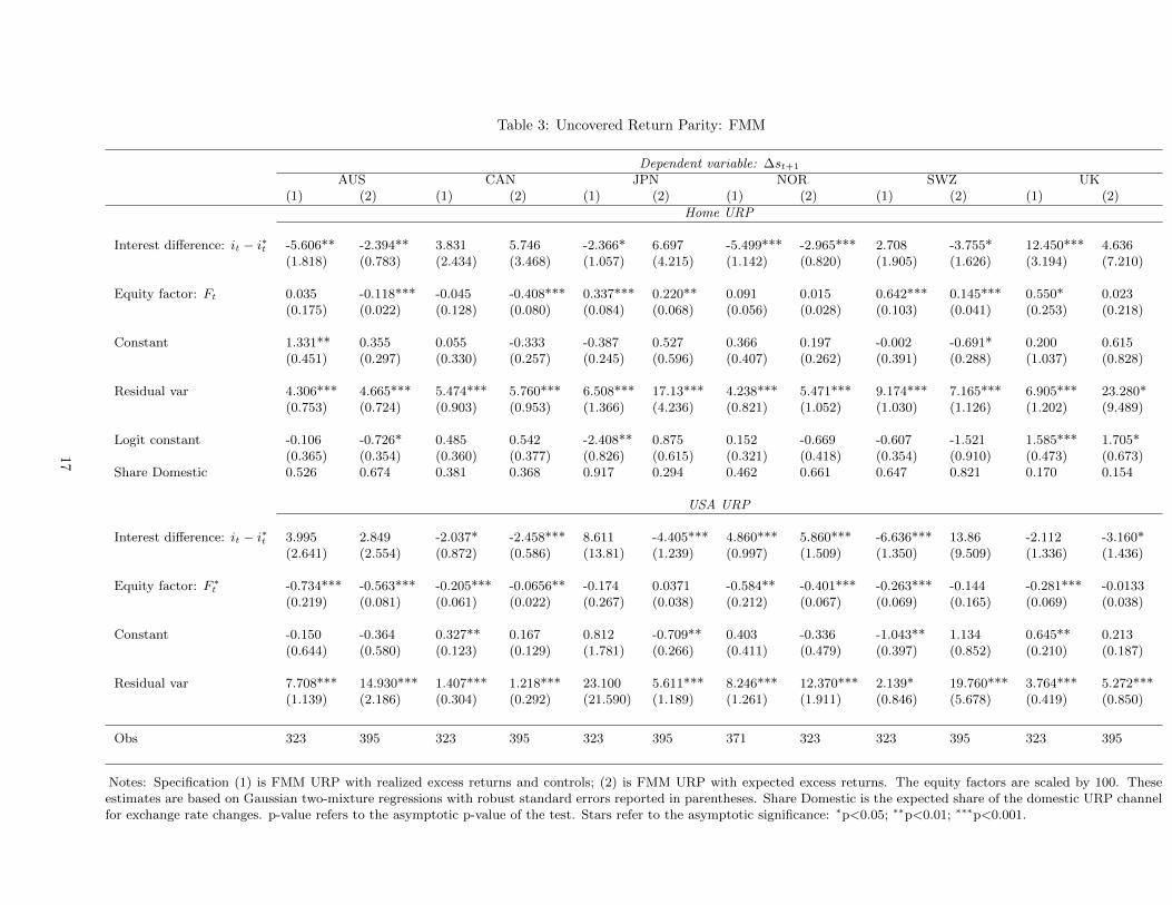
Table 3: Uncovered Return Parity: FMM

Dependent variable: ∆st+1

AUS CAN JPN NOR SWZ UK(1) (2) (1) (2) (1) (2) (1) (2) (1) (2) (1) (2)

Home URP

Interest difference: it − i∗t -5.606** -2.394** 3.831 5.746 -2.366* 6.697 -5.499*** -2.965*** 2.708 -3.755* 12.450*** 4.636(1.818) (0.783) (2.434) (3.468) (1.057) (4.215) (1.142) (0.820) (1.905) (1.626) (3.194) (7.210)

Equity factor: Ft 0.035 -0.118*** -0.045 -0.408*** 0.337*** 0.220** 0.091 0.015 0.642*** 0.145*** 0.550* 0.023(0.175) (0.022) (0.128) (0.080) (0.084) (0.068) (0.056) (0.028) (0.103) (0.041) (0.253) (0.218)

Constant 1.331** 0.355 0.055 -0.333 -0.387 0.527 0.366 0.197 -0.002 -0.691* 0.200 0.615(0.451) (0.297) (0.330) (0.257) (0.245) (0.596) (0.407) (0.262) (0.391) (0.288) (1.037) (0.828)

Residual var 4.306*** 4.665*** 5.474*** 5.760*** 6.508*** 17.13*** 4.238*** 5.471*** 9.174*** 7.165*** 6.905*** 23.280*(0.753) (0.724) (0.903) (0.953) (1.366) (4.236) (0.821) (1.052) (1.030) (1.126) (1.202) (9.489)

Logit constant -0.106 -0.726* 0.485 0.542 -2.408** 0.875 0.152 -0.669 -0.607 -1.521 1.585*** 1.705*(0.365) (0.354) (0.360) (0.377) (0.826) (0.615) (0.321) (0.418) (0.354) (0.910) (0.473) (0.673)

Share Domestic 0.526 0.674 0.381 0.368 0.917 0.294 0.462 0.661 0.647 0.821 0.170 0.154

USA URP

Interest difference: it − i∗t 3.995 2.849 -2.037* -2.458*** 8.611 -4.405*** 4.860*** 5.860*** -6.636*** 13.86 -2.112 -3.160*(2.641) (2.554) (0.872) (0.586) (13.81) (1.239) (0.997) (1.509) (1.350) (9.509) (1.336) (1.436)

Equity factor: F ∗t -0.734*** -0.563*** -0.205*** -0.0656** -0.174 0.0371 -0.584** -0.401*** -0.263*** -0.144 -0.281*** -0.0133

(0.219) (0.081) (0.061) (0.022) (0.267) (0.038) (0.212) (0.067) (0.069) (0.165) (0.069) (0.038)

Constant -0.150 -0.364 0.327** 0.167 0.812 -0.709** 0.403 -0.336 -1.043** 1.134 0.645** 0.213(0.644) (0.580) (0.123) (0.129) (1.781) (0.266) (0.411) (0.479) (0.397) (0.852) (0.210) (0.187)

Residual var 7.708*** 14.930*** 1.407*** 1.218*** 23.100 5.611*** 8.246*** 12.370*** 2.139* 19.760*** 3.764*** 5.272***(1.139) (2.186) (0.304) (0.292) (21.590) (1.189) (1.261) (1.911) (0.846) (5.678) (0.419) (0.850)

Obs 323 395 323 395 323 395 371 323 323 395 323 395

Notes: Specification (1) is FMM URP with realized excess returns and controls; (2) is FMM URP with expected excess returns. The equity factors are scaled by 100. Theseestimates are based on Gaussian two-mixture regressions with robust standard errors reported in parentheses. Share Domestic is the expected share of the domestic URP channelfor exchange rate changes. p-value refers to the asymptotic p-value of the test. Stars refer to the asymptotic significance: ∗p<0.05; ∗∗p<0.01; ∗∗∗p<0.001.

17

To evaluate whether there is empirical support for our mixture model, and potential misspecification

more generally, we also compare our mixture model estimates with those obtained from the single equation

URP specifications we described above. We report the AIC and BIC in Table 4 to evaluate whether including

additional information from the foreign country’s URP condition improves the statistical properties of the

model. We report two model specifications: URP estimated by OLS and URP estimated by FMM. The AIC

results unambiguously support URP over UIP. The results for AIC also unambiguously support FMM over

OLS. However, for Japan and Switzerland the BIC suggests that OLS UIP may be preferred. The difference

between AIC and BIC for Japan and Switzerland is due to the difference 2k − ln(n)k penalty term applied

to the number of parameters, k, in the FMM URP, k = 9, versus UIP, k = 3. We remind the reader that

UIP was rejected as a nested hypothesis for Japan and Switzerland. Nevertheless, the BIC criterion also

marginally favours OLS URP over FMM URP for Japan and Switzerland. Again, the difference appears

due to the number of parameters estimated under FMM, k = 9, versus OLS, k = 4, which suggests that

the parameter restrictions embedded in OLS may be reasonable. We conclude that URP appears to have

support in the data we examine and that FMM appears on balance the preferred specification. We also

note that our empirical investigation of URP is, by design, focussed only on portfolios comprised of equities

and short-term treasuries. It would seem probable that broader portfolios would yield even more conclusive

evidence for URP but that investigation is beyond the scope of this paper.

5.3 The Commodity Channel

The URP condition implies that any asset that is correlated with domestic equity returns should also affect

currency returns through the equity channel. An example of such potential assets are commodities. Kilian

and Park (2009) and Ready (2017) argue that oil prices affect equity returns; so if the URP channel we

propose is valid, then oil prices should affect exchange rates through this channel. URP is unlike UIP, where

there is no theoretical possibility for exchange rate returns to depend directly on oil prices.

We use the oil-equity factors described above to examine, using FMM, whether expectations over oil

price changes affect expected exchange rate returns. We estimate Equation (9) replacing the equity factor

with the oil-equity factor. The oil-equity factor captures the extent to which current equity prices reflect the

next month’s WTI change. It is also a measure of the oil sensitivity of domestic equity returns.13

Table 5 presents FMM estimates of URP using the oil-equity factor. The results suggest that the countries

we examine can be clustered into three groups for the domestic channel of URP: the Australian and Canadian

expected exchange rates rise (fall) with increases (decreases) in the oil-equity factor; the Japanese and Swiss

expected exchange rates fall (rise) with increases (decreases) in the oil-equity factor; and the Norwegian and

UK expected exchange rates are insignificantly affected by the oil-equity factor. For the US channel of URP,

13We also investigate an oil-equity factor constructed using contemporaneous equity excess returns and oil price changes andfind similar results.

18

Table 4: Information Criterion for URP

AIC BIC

AUSOLS UIP 2057.335 2069.272OLS URP 2028.794 2044.710FMM URP 1996.406 2032.216

CANOLS UIP 1660.400 1672.337OLS URP 1644.527 1660.442FMM URP 1592.099 1627.909

JPNOLS UIP 2050.974 2062.910OLS URP 2052.970 2068.885FMM URP 2034.272 2070.082

NOROLS UIP 1920.813 1932.561OLS URP 1915.937 1931.602FMM URP 1888.969 1924.214

SWZOLS UIP 2075.235 2087.172OLS URP 2076.445 2092.361FMM URP 2062.569 2098.379

UKOLS UIP 1977.290 1989.226OLS URP 1976.583 1992.499FMM URP 1952.573 1988.383

Notes: The AIC and BIC refer to the Akaikeand Bayes information criterion from Table 1and from columns labelled (2) in Tables 2 and3.

19

the expected exchange rates fall with increases in the oil-equity factor for all countries except Japan (recall

that the approximation ∆s∗t+1 = −∆st+1 implies that interpretation of the coefficient on F oil,∗t is the inverse

of that for F oilt ).

5.4 Robustness

One concern with the results for Norway and the UK presented in Tables 3 and 5 is that both countries

have experienced structural changes that may affect URP over the sample period. Since June 2001, the

Norwegian stock exchange, the Oslo Bors, has been dominated by a single firm, Statoil, which accounts for

roughly 20–25% of the total market capitalization. Given the construction of our equity factors, the entry

of a dominant firm could be problematic for the equally weighted market expected return. To account for

the Statoil effect, we split our sample for Norway at June 2001 and re-estimate the equity and oil-equity

factors for the post-June 2001 period. For the UK, the exchange rate crisis of 1992 saw the UK exit the

currency corridor preceding the introduction of the Euro. Expected currency returns under a managed float

confound at least two dynamics: the role of fundamental factors such as the URP and the expectation of

the continuance of the managed float. To account for the ERM effect, we split our sample for the UK at

September 1992. However, we do not re-estimate the equity factor or oil-equity factor for only the post ERM

period since there is no reason to believe that the expectations embedded in the existing equities should have

been affected.

Table 6 presents FMM estimates for the equity and oil-equity factors for Norway post June 2001 and the

UK post September 1992. In each case, the domestic equity or oil-equity factor is significant. In particular,

the results for the oil-equity factor suggest that Norway and the UK should be considered similar to Australia

and Canada in so much as expected exchange rates rise (fall) with increases (decreases) in the oil-equity

factor. There is also evidence that the expected exchange rates fall with increases in the oil-equity factor for

the US channel. Overall, the estimates also suggest that the majority of exchange rate movements in the

expected exchange rates are driven by the US channel.

5.5 Posterior Mixture Probabilities

One feature of the FMM methodology is that it yields estimates of the posterior probability of group

membership. Figure 1 presents the estimated posterior probabilities for the domestic URP share of the

expected exchange rate movements using the equity factor URP specification from columns labelled (2) in

Table 3. Two features stand out. First, the estimated posterior share is volatile for all of the countries in the

sample. The second common feature is that the posterior probabilities appear to be on average in the range

0.7 − 0.9 for Australia, Norway and Switzerland or in the range 0.1 − 0.3 for Canada, Japan and the UK.

Both observations support the central thesis of this paper that exchange rate models from the perspective of

20

Table 5: Uncovered Return Parity: Oil-Equity Factor

Dependent variable: ∆st+1

AUS CAN JPN NOR SWZ UK

Home URP

Interest difference: it − i∗t 4.738 10.820** 6.288 -5.634*** -4.489** -2.800(4.123) (4.190) (4.079) (1.500) (1.484) (1.466)

Oil factor: F oilt -0.198*** -0.231*** 0.105*** 0.012 0.035** -0.026

(0.058) (0.027) (0.029) (0.018) (0.013) (0.015)

Constant -1.089 -0.285 0.850 0.387 -0.992** -0.027(0.904) (0.397) (0.632) (0.316) (0.376) (0.234)

Residual var 14.170*** 5.887*** 16.240*** 4.854*** 7.066*** 4.390***(3.681) (1.140) (3.992) (1.096) (1.474) (0.910)

Logit constant 0.929 0.925* 0.939 0.221 -0.860 -1.587*(0.484) (0.449) (0.492) (0.361) (0.674) (0.717)

Share Domestic 0.283 0.284 0.281 0.445 0.703 0.830

USA URP

Interest difference: it − i∗t -3.389 -1.508* -3.558** 4.444*** 7.781 14.040(1.746) (0.712) (1.095) (0.919) (4.337) (9.636)

Oil factor: F oil,∗t -0.107*** -0.048** -0.035 -0.193*** -0.117** -0.165***

(0.031) (0.016) (0.019) (0.021) (0.043) (0.036)

Constant 0.484 -0.047 -0.602* -0.506 1.370 -0.074(0.444) (0.149) (0.257) (0.303) (0.765) (1.047)

Residual var 4.942*** 1.971*** 4.897*** 7.576*** 9.393* 7.997*(0.875) (0.491) (0.760) (1.162) (4.383) (3.336)

Obs 324 324 324 324 324 324

Notes: These estimates are based on Gaussian two-mixture regressions with robust standard errorsreported in parentheses. The equity factors are scaled by 100. Share Domestic is the expected shareof the domestic URP channel for exchange rate changes. Stars refer to the asymptotic significance:∗p<0.05; ∗∗p<0.01; ∗∗∗p<0.001.

21

Table 6: Statoil and the Exchange Rate Mechanism

Dependent variable: ∆st+1

NOR Post-Statoil UK Post-ERM NOR Post-Statoil UK Post-ERMEquity Factor Oil Factor

Home URP

Interest difference: it − i∗t 0.845 23.430*** -7.772** 17.280**(5.381) (4.927) (2.649) (5.507)

Equity or oil factor: Ft or F oilt -0.368*** -0.226** -0.134** -0.119**

(0.664) (0.0703) (4.676) (4.315)

Constant -0.302 0.197 -0.811 -0.183(1.044) (1.123) (0.537) (1.121)

Residual var 7.405*** 11.410** 5.589*** 9.841**(2.207) (3.534) (1.270) (3.292)

Logit constant 0.617 1.824*** 0.503 1.524**(0.521) (0.450) (0.532) (0.464)

Share Domestic 0.350 0.139 0.377 0.179

USA URP

Interest difference: it − i∗t -2.818 -1.091 3.464 -1.510(2.575) (2.085) (2.175) (2.249)

Equity or oil factor: F ∗t or F oil,∗

t -0.608 -0.020 -0.187*** -0.381*(0.725) (0.033) (2.415) (1.865)

Constant 0.007 -0.074 0.200 -0.110(0.568) (0.242) (0.432) (0.280)

Residual var 8.523*** 4.141*** 7.055*** 3.892***(1.939) (0.569) (1.361) (0.594)

Obs 185 292 185 292

Notes: These estimates are based on Gaussian two-mixture regressions with robust standard errors reported inparentheses. The equity factors are scaled by 100. Share Domestic is the expected share of the domestic URPchannel for exchange rate changes. Stars refer to the asymptotic significance: ∗p<0.05; ∗∗p<0.01; ∗∗∗p<0.001.

22

one country are essentially misspecified. Of perhaps greater interest is that to better understand exchange

rate movements, it would appear necessary to investigate the economic forces that cause the sharp changes

in the estimated posterior share. We leave such investigation for future research.

6 Conclusion

In this paper, we have made two contributions to understanding currency markets. First, we have suggested

an augmented parity condition, URP, to help to understand the driving factors of currency returns. We show

empirical evidence that our portfolio channel is operative and that it can go some way to understanding

exchange rate changes.

Second, both as part of a logical test of URP and also of interest in its own right, we have proposed

a channel through which commodity prices affect currency markets. We show that countries can be differ-

entiated in terms of the sensitivity and direction in which commodity price changes affect their bilateral

USD exchange rates. In particular, we find evidence that Australia and Canada, and probably Norway and

the UK, are commodity currencies. We also find evidence that the Yen and Swiss France are sensitive to

commodity prices in the opposite direction.

Recently, Chien, Lustig, and Naknoi (2015) and Dou and Verdelhan (2015) have suggested that differences

across investors may play a valuable role in explaining currency markets. We note that our setting may

possibly be extended to include incomplete markets, as the portfolio uncertainty wedge we propose would

also drive a wedge in the exchange rate in an incomplete-market setting. Indeed, the scope for future

research appears to include a number of possible avenues in addition to risk, for example: time-varying

portfolio composition effects; time-varying US URP shares; and even simply extending across additional

assets, maturities and countries.

23

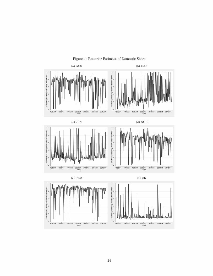
Figure 1: Posterior Estimate of Domestic Share

(a) AUS

0.2

.4.6

.81

Post

erio

r pro

babi

lity

of d

omes

tic U

RP

shar

e

1985m1 1990m1 1995m1 2000m1 2005m1 2010m1 2015m1date

(b) CAN

0.2

.4.6

.81

Post

erio

r pro

babi

lity

of d

omes

tic U

RP

shar

e1985m1 1990m1 1995m1 2000m1 2005m1 2010m1 2015m1

date

(c) JPN

0.2

.4.6

.81

Post

erio

r pro

babi

lity

of d

omes

tic U

RP

shar

e

1985m1 1990m1 1995m1 2000m1 2005m1 2010m1 2015m1date

(d) NOR

0.2

.4.6

.81

Post

erio

r pro

babi

lity

of d

omes

tic U

RP

shar

e

1985m1 1990m1 1995m1 2000m1 2005m1 2010m1 2015m1date

(e) SWZ

0.2

.4.6

.81

Post

erio

r pro

babi

lity

of d

omes

tic U

RP

shar

e

1985m1 1990m1 1995m1 2000m1 2005m1 2010m1 2015m1date

(f) UK

0.2

.4.6

.81

Post

erio

r pro

babi

lity

of d

omes

tic U

RP

shar

e

1985m1 1990m1 1995m1 2000m1 2005m1 2010m1 2015m1date

24

References

Alvarez, F., A. Atkeson, and P. J. Kehoe (2002): “Money, interest rates, and exchange rates with

endogenously segmented markets,” Journal of Political Economy, 101(1), 73–112.

Bali, T. G., R. F. Engle, and S. Murray (2016): Empirical asset pricing: The cross section of stock

returns. John Wiley & Sons.

Bilson, J. F. O. (1981): “The ‘Speculative Efficiency’ Hypothesis,” The Journal of Business, 54(3), 435–

451.

Cashin, P., L. F. Cespedes, and R. Sahay (2004): “Commodity currencies and the real exchange rate,”

Journal of Development Economics, 75(1), 239–268.

Cenedese, G., R. Payne, L. Sarno, and G. Valente (2016): “What do stock markets tell us about

exchange rates?,” Review of Finance, 20(3), 1045–1080.

Chen, N.-F., R. Roll, and S. A. Ross (1986): “Economic forces and the stock market,” Journal of

Business, 59(3), 383–403.

Chen, S.-S. (2016): “Commodity prices and related equity prices,” Canadian Journal of Economics/Revue

canadienne d’economique, 49(3), 949–967.

Chen, Y.-c., and K. Rogoff (2003): “Commodity currencies,” Journal of International Economics, 60(1),

133–160.

Chen, Y.-C., K. S. Rogoff, and B. Rossi (2010): “Can exchange rates forecast commodity prices?,”

The Quarterly Journal of Economics, 125(3), 1145–1194.

Chien, Y., H. N. Lustig, and K. Naknoi (2015): “Why are exchange rates so smooth? A segmented

asset markets explanation,” Working paper.

Chui, A. C., S. Titman, and K. J. Wei (2010): “Individualism and momentum around the world,” The

Journal of Finance, 65(1), 361–392.

Compiani, G., and Y. Kitamura (2016): “Using mixtures in econometric models: A brief review and

some new results,” The Econometrics Journal, 19(3), C95–C127.

Deb, P. (2012): “FMM: Stata module to estimate finite mixture models,”

https://EconPapers.repec.org/RePEc:boc:bocode:s456895, [Online; accessed 26-April-2018].

Dou, W. W., and A. Verdelhan (2015): “The volatility of international capital flows and foreign assets,”

Discussion paper, Working Paper MIT Sloan.

25

Engel, C. (1996): “The forward discount anomaly and the risk premium: A survey of recent evidence,”

Journal of Empirical Finance, 3(2), 123–192.

(2014): “Exchange rates and interest parity,” Handbook of International Economics, 4, 453 – 522.

(2016): “Exchange rates, interest rates, and the risk premium,” The American Economic Review,

106(2), 436–474.

Fama, E. F. (1984): “Forward and spot exchange rates,” Journal of Monetary Economics, 14(3), 319–338.

Ferraro, D., K. Rogoff, and B. Rossi (2015): “Can oil prices forecast exchange rates? An empirical

analysis of the relationship between commodity prices and exchange rates,” Journal of International

Money and Finance, 54, 116–141.

Fratzscher, M., D. Schneider, and I. Van Robays (2014): “Oil prices, exchange rates and asset

prices,” Working paper.

Guerin, P., D. Leiva-Leon, and M. Marcellino (2016): “Markov-switching three-pass regression filter,”

Working paper.

Guvenen, F., and B. Kuruscu (2006): “Does market incompleteness matter for asset prices?,” Journal

of the European Economics Association, 4, 484–492.

Gyntelberg, J., M. Loretan, and T. Subhanij (2018): “Private information, capital flows, and ex-

change rates,” Journal of International Money and Finance, 81, 40–55.

Habib, M. M., S. Butzer, and L. Stracca (2016): “Global exchange rate configurations: Do oil shocks

matter?,” IMF Economic Review, 64(3), 443–470.

Hau, H., and H. Rey (2006): “Exchange rates, equity prices, and capital flows,” Review of Financial

Studies, 19(1), 273–317.

Hou, K., G. A. Karolyi, and B.-C. Kho (2011): “What factors drive global stock returns?,” Review of

Financial Studies, 24(8), 2527–2574.

Huang, D., and J. Miao (2018): “Oil driven stock price momentum,” Working paper.

Ince, O. S., and R. B. Porter (2006): “Individual equity return data from Thomson Datastream: Handle

with care!,” Journal of Financial Research, 29(4), 463–479.

Jones, C. M., and G. Kaul (1996): “Oil and the stock markets,” The Journal of Finance, 51(2), 463–491.

26

Kelly, B., and S. Pruitt (2013): “Market expectations in the cross-section of present values,” The Journal

of Finance, 68(5), 1721–1756.

(2015): “The three-pass regression filter: A new approach to forecasting using many predictors,”

Journal of Econometrics, 186(2), 294–316.

Kilian, L., and C. Park (2009): “The impact of oil price shocks on the US stock market,” International

Economic Review, 50(4), 1267–1287.

Kremens, L., and I. Martin (2017): “The quanto theory of exchange rates,” Working paper.

Lee, K.-H. (2011): “The world price of liquidity risk,” Journal of Financial Economics, 99(1), 136–161.

Lu, H., and B. Jacobsen (2016): “Cross-asset return predictability: Carry trades, stocks and commodi-

ties,” Journal of International Money and Finance, 64, 62–87.

Lustig, H., and A. Verdelhan (2007): “The cross section of foreign currency risk premia and consumption

growth risk,” The American Economic Review, 97(1), 89–117.

Meese, R. A., and K. Rogoff (1983): “Empirical exchange rate models of the seventies: Do they fit out

of sample?,” Journal of International Economics, 14(1-2), 3–24.

Passari, E. (2017): “Exchange rates and commodity prices,” Working paper.

Pavlova, A., and R. Rigobon (2007): “Asset prices and exchange rates,” Review of Financial Studies,

20(4), 1139–1180.

Ready, R. (2017): “Oil prices and the stock market,” Review of finance, Forthcoming.

Ready, R., N. Roussanov, and C. Ward (2017): “After the tide: Commodity currencies and global

trade,” Journal of Monetary Economics, 85, 69–86.

Sadorsky, P. (1999): “Oil price shocks and stock market activity,” Energy economics, 21(5), 449–469.

Siegel, J. J. (1972): “Risk, interest rates and the forward exchange,” The Quarterly Journal of Economics,

86(2), 303–309.

Van Nieuwerburgh, S., and L. Veldkamp (2009): “Information immobility and the home bias puzzle,”

The Journal of Finance, 64(3), 1187–1215.

Vissing-Jørgensen, A. (2002): “Limited asset market participation and the elasticity of intertemporal

substitution,” Journal of Political Economy, 110, 825–853.

27

Wong, C. S., and W. K. Li (2001): “On a logistic mixture autoregressive model,” Biometrika, 88(3),

833–846.

Zervou, A. (2013): “Financial market segmentation, stock market volatility and the role of monetary

policy,” European Economic Review, 63, 256–272.

28

A Appendix

A.1 Summary Statistics

Table 7: Summary Statistics

AUS CAN JPN NOR SWZ UKInterest rate differential : it − i∗t

mean 0.245 0.055 -0.180 0.173 -0.131 0.138sd 0.197 0.110 0.173 0.231 0.178 0.157skew 0.861 0.505 -0.203 1.364 0.317 0.916kurt 0.660 0.813 -1.206 4.721 0.264 0.047AR(1) 0.974 0.944 0.984 0.919 0.976 0.965adf -3.350 -2.540 -2.599 -3.016 -3.070 -4.434p.value 0.063 0.349 0.324 0.148 0.125 0.010n 397 397 397 373 397 397

Equity returns : rtmean 0.900 0.772 0.302 0.967 0.800 0.853sd 4.894 4.111 5.580 6.616 4.555 4.517skew -3.336 -1.374 -0.362 -1.070 -1.262 -1.146kurt 32.379 6.338 1.134 3.330 4.798 5.197AR(1) 0.002 0.129 0.114 0.148 0.163 0.048adf -7.731 -7.580 -6.516 -7.621 -6.549 -7.378p.value 0.010 0.010 0.010 0.010 0.010 0.010n 395.000 395.000 395.000 395.000 395.000 395.000

Pseudo Equity premium : rt+1 − itmean 0.320 0.383 0.148 0.480 0.597 0.380sd 4.888 4.123 5.584 6.625 4.559 4.512skew -3.443 -1.391 -0.393 -1.220 -1.284 -1.212kurt 33.361 6.396 1.160 3.736 4.841 5.429AR(1) 0.002 0.134 0.116 0.164 0.164 0.046adf -7.645 -7.465 -6.486 -7.266 -6.473 -7.306p.value 0.010 0.010 0.010 0.010 0.010 0.010n 395.000 395.000 395.000 371.000 395.000 395.000

Exchange rate : ∆stmean 0.048 0.011 -0.185 0.011 -0.208 0.027sd 3.436 2.129 3.262 3.215 3.373 2.947skew 0.682 0.614 -0.357 0.459 -0.042 0.306kurt 2.583 4.997 1.458 1.183 0.784 2.183AR(1) 0.055 -0.042 0.041 0.010 -0.011 0.073adf -7.067 -6.982 -7.138 -7.467 -7.272 -7.948p.value 0.010 0.010 0.010 0.010 0.010 0.010n 396 396 396 396 396 396

Notes: This table reports monthly summary statistics based on the full-sample estimates using interest rate differential, equity returns, equity pre-mium, change in exchange rate. We compute change in exchange rate as logdifferences in nominal exchange. The equity return is the log differences ofthe country index. We compute the interest rate differential with respect tothe USA. All variables are multiplied by 100.

A.2 Estimation of the Three-pass Equity Factor

We use monthly individual stocks data listed on the major exchange in each country. These stock exchanges

are: Australia, Toronto, Oslo, NYSE, Tokyo, London and Zurich. All these data come from Datastream and

cover the period January 1984 to December 2016 and are denominated in local currency. To mitigate the

effects of outliers, we apply a couple of screening procedures common in the literature (Ince and Porter 2006,

Chui, Titman, and Wei 2010, Hou, Karolyi, and Kho 2011, Lee 2011, Bali, Engle, and Murray 2016). First,

we truncate small firms in each country by treating as missing data the returns of the 5% lowest market

capitalization. This imputation procedure is done period by period. Second, we apply a winzorization

29

Table 8: Correlations between Exchange Rates, Interest Rates andEquity Returns

AUS CAN JPN NOR SWZ UKInterest rate differential: it − i∗t

Equity returns 0.025 -0.051 0.009 -0.091 -0.054 0.016Equity premium -0.024 -0.084 0.001 -0.123 -0.067 -0.036Exchange rate -0.053 0.005 -0.083 -0.007 -0.070 -0.066

Equity returns: rtInterest rate differential 0.025 -0.051 0.009 -0.091 -0.054 0.016Equity premium 0.998 0.998 0.999 0.999 0.999 0.997Exchange rate -0.350 -0.413 0.132 -0.107 0.258 0.080

Pseudo Equity premium: rt+1 − itInterest rate differential -0.024 -0.084 0.001 -0.123 -0.067 -0.036Equity returns 0.998 0.998 0.999 0.999 0.999 0.997Exchange rate -0.352 -0.410 0.136 -0.099 0.260 0.084

Exchange rate: ∆stInterest rate differential -0.053 0.005 -0.083 -0.007 -0.070 -0.066Equity returns -0.350 -0.413 0.132 -0.107 0.258 0.080Equity premium -0.352 -0.410 0.136 -0.099 0.260 0.084

Notes: This table reports monthly correlation based on the full-sample estimatesusing interest rate differential, equity returns, equity premium, change in exchangerate. We compute change in exchange rate as log differences in nominal exchange.The equity return is the log differences of the country index. We compute the interestrate differential with respect to the USA.

technique by imputing the 0.1% lowest value to the 0.1% quantile threshold and the 99.9% highest to

the 99.9% quantile threshold (Bali, Engle, and Murray 2016, Chapter 1). Following the truncation and

winzorization procedure, we keep firms that have more than 10% of data (i.e., firms with less than 90% of

missing data) or alternatively firms with at least 40 observations. And finally, we treated as missing data

any return above 300% that is reversed within one month.

30

Table 9: Summary Statistics on the Size of the Cross-Section of Equity Returns by Country and Year

AUS CAN JPN NOR SWZ UK USAyear min median max min median max min median max min median max min median max min median max min median max1984 43 45 45 84 86 91 673 674 674 16 16 16 44 44 46 218 232 236 693 709 7241985 45 45 46 93 94 95 674 674 675 16 18 18 46 48 48 236 242 245 725 738 7591986 46 46 49 95 102 117 675 675 675 18 20 21 48 52 61 247 255 261 763 786 8331987 49 55 59 119 124 131 675 676 762 21 21 21 64 68 75 268 272 276 845 871 9051988 59 92 125 132 136 371 763 1061 1106 21 21 21 77 78 85 276 290 303 908 922 9371989 127 157 171 378 400 456 1113 1162 1304 21 22 22 85 91 93 308 312 319 941 950 9661990 171 176 181 464 610 623 1313 1432 1473 22 23 23 93 112 112 323 324 324 970 990 10001991 181 182 188 625 644 667 1480 1566 1610 23 24 25 112 112 115 325 326 328 1002 1026 10621992 188 197 197 667 685 701 1616 1628 1649 25 26 32 115 115 119 328 328 333 1074 1124 11571993 197 202 211 703 718 736 1651 1664 1699 32 32 32 119 122 123 334 340 346 1167 1222 12861994 215 237 255 742 769 799 1712 1746 1828 33 36 38 123 126 126 347 358 367 1297 1356 13971995 260 266 274 801 814 839 1843 1892 1956 38 41 43 127 130 133 372 378 403 1404 1435 15041996 280 428 444 846 867 899 1967 2000 2070 45 48 49 133 134 139 408 422 445 1515 1562 16361997 444 464 476 908 954 994 2081 2106 2166 49 56 62 140 141 143 451 466 479 1649 1698 17671998 480 496 505 1006 1052 1087 2173 2184 2215 63 66 71 143 148 155 483 491 499 1778 1842 18811999 511 517 543 1092 1117 1173 2224 2245 2286 71 72 74 155 158 164 500 504 515 1886 1942 20272000 561 594 632 1183 1210 1310 2297 2337 2408 74 77 78 164 170 176 522 555 581 2031 2080 21362001 644 662 675 1321 1368 1390 2431 2472 2531 79 82 84 176 180 181 589 606 620 2143 2168 22002002 680 698 718 1391 1415 1441 2548 2588 2624 84 87 88 181 182 183 627 649 662 2204 2232 22612003 720 728 763 1446 1466 1489 2637 2671 2706 88 89 89 184 185 185 666 675 693 2266 2281 23152004 783 816 864 1496 1535 1580 2725 2772 2830 90 94 96 185 187 188 699 726 787 2327 2372 24302005 886 935 981 1594 1651 1707 2846 2892 2945 98 104 112 189 192 196 811 884 947 2441 2495 25562006 997 1044 1110 1722 1785 1847 2964 3025 3084 113 118 128 197 200 203 967 1016 1062 2563 2610 26712007 1136 1213 1304 1858 1940 2045 3106 3159 3198 129 139 146 203 207 212 1075 1112 1151 2688 2756 28172008 1345 1386 1404 2068 2161 2233 3206 3224 3236 148 152 155 217 224 228 1156 1174 1188 2834 2862 28852009 1404 1411 1428 2233 2265 2306 3244 3258 3271 155 155 156 229 230 232 1190 1193 1197 2886 2894 29242010 1443 1462 1492 2313 2374 2446 3273 3288 3299 156 160 165 232 234 236 1199 1220 1247 2933 2986 30322011 1520 1569 1607 2473 2556 2636 3304 3320 3343 166 170 173 236 238 242 1253 1271 1297 3045 3108 31552012 1619 1640 1660 2646 2763 2857 3353 3369 3395 174 174 176 242 243 246 1298 1314 1332 3166 3228 32792013 1671 1684 1693 2870 2912 2932 3410 3432 3444 176 178 180 246 247 247 1340 1360 1375 3290 3376 34392014 1681 1689 1693 2925 2933 2936 3443 3444 3444 180 180 180 247 247 247 1374 1374 1375 3438 3439 34392015 1677 1680 1682 2914 2923 2928 3442 3444 3444 180 180 180 247 247 247 1370 1372 1375 3436 3438 34392016 1672 1675 1677 2914 2925 2928 3442 3442 3442 178 179 180 247 247 247 1368 1369 1371 3432 3434 34362017 1673 1673 1673 2926 2926 2926 3442 3442 3442 180 180 180 247 247 247 1369 1369 1369 3431 3431 3431

Notes: This table reports the minimum, median and maximum number of equity returns in the sample per country and year.

31

Table 10: Summary Statistics of Stock Returns by Country and Year

AUS CAN JPN NOR SWZ UK USAYear mean sd mean sd mean sd mean sd mean sd mean sd mean sd1984 0.623 4.746 -0.975 3.340 0.973 3.736 2.326 7.926 0.019 2.133 1.591 4.301 -0.226 4.0281985 2.522 3.201 2.365 2.264 1.416 1.711 0.864 7.157 3.676 3.087 1.789 3.263 2.315 3.9191986 2.729 4.980 1.456 2.731 1.876 4.799 -3.565 3.768 1.253 4.271 2.453 3.211 0.715 4.2431987 -2.228 13.697 -0.836 10.175 1.751 5.663 0.637 8.585 -2.265 9.967 1.426 11.275 -0.462 10.8071988 -0.715 4.738 -1.361 3.117 2.196 4.572 1.972 4.949 2.123 3.099 0.931 2.829 1.535 2.9721989 -0.777 5.079 -1.363 5.671 3.429 3.288 4.287 6.812 0.693 2.620 0.693 4.741 1.353 2.7141990 -4.361 3.180 -2.912 5.848 -3.705 11.656 -0.567 6.756 -1.979 4.925 -2.236 4.509 -1.600 5.8191991 2.941 3.429 -1.136 3.220 -0.554 8.213 -0.660 6.483 -0.360 3.497 0.775 5.001 2.847 3.8801992 -0.544 3.493 1.142 6.424 -2.880 5.436 -4.536 6.301 -0.817 2.904 0.320 5.976 1.334 3.4161993 3.992 5.048 4.152 4.896 0.536 8.254 5.841 6.306 3.547 2.501 3.361 2.541 1.423 2.3141994 -0.901 5.356 -2.053 4.713 1.430 4.691 0.214 4.415 -0.391 3.028 -0.242 4.212 -0.595 2.5311995 0.036 3.760 0.655 3.945 -0.681 6.056 1.577 2.677 0.487 2.151 0.930 1.886 1.881 2.0331996 2.086 3.929 2.663 7.453 -0.898 4.785 2.952 2.764 0.960 2.024 0.949 2.357 1.206 3.7351997 -2.776 5.484 -3.858 6.147 -5.071 5.978 2.029 4.720 2.265 2.807 0.378 2.126 1.700 4.0901998 -1.852 6.511 -4.375 7.324 -0.141 7.787 -4.229 6.704 0.926 7.072 -1.446 5.351 -0.683 7.0231999 2.612 4.002 -0.063 3.965 1.342 6.431 3.141 4.298 1.643 2.555 2.895 3.333 0.501 3.5912000 -2.528 10.849 -1.225 11.608 -1.258 4.671 -0.285 4.568 0.712 2.397 -0.638 3.323 -0.982 4.7802001 -2.217 6.577 -3.450 5.639 -0.997 4.655 -1.799 5.669 -2.645 5.953 -2.035 7.193 0.636 6.9772002 -1.704 3.451 -0.322 6.328 -1.294 3.846 -4.120 6.390 -2.752 5.651 -2.773 5.205 -1.531 5.9752003 2.064 5.886 3.615 4.453 2.771 3.851 4.382 5.523 2.034 4.204 2.844 4.697 3.732 3.9402004 0.245 4.021 -0.427 3.611 1.968 5.770 2.547 5.892 1.057 2.570 0.920 2.950 1.405 3.7592005 -0.631 4.147 0.517 4.234 3.463 2.747 3.593 4.778 2.084 2.546 0.577 3.589 0.239 3.4512006 1.494 4.118 1.756 5.871 -2.008 4.643 1.941 3.373 2.113 2.750 0.479 2.896 1.118 3.2022007 -0.077 4.428 -0.733 5.412 -2.069 3.763 0.063 3.204 0.589 3.709 -1.245 3.334 -0.507 3.3432008 -9.489 9.506 -10.074 12.461 -4.272 7.138 -8.151 10.043 -4.308 6.529 -6.880 7.753 -5.452 9.1262009 3.757 5.982 4.223 4.552 0.742 6.351 2.086 5.688 1.530 5.623 2.817 6.024 2.658 8.3892010 0.134 6.417 2.113 5.389 0.485 6.037 0.592 5.588 1.054 2.683 1.244 4.116 1.487 6.3022011 -3.435 5.325 -3.480 5.321 -0.519 3.131 -3.339 5.031 -1.749 3.469 -2.105 3.315 -1.034 5.7802012 -1.930 5.098 -3.077 5.446 1.340 5.421 0.197 4.857 0.478 2.269 -0.033 3.840 1.006 3.7052013 -2.069 6.553 -3.309 4.453 3.317 5.481 1.586 3.101 1.111 1.704 0.990 2.906 2.598 2.7992014 -2.277 3.974 -1.879 5.781 0.997 2.936 -0.869 2.796 0.729 1.218 -1.474 2.103 -0.007 3.3002015 -0.885 3.826 -2.989 3.135 0.581 3.784 -1.552 3.333 0.122 2.935 -1.424 2.706 -1.149 3.7512016 0.426 3.435 3.078 4.894 0.326 4.916 0.820 3.855 0.407 1.823 -0.095 2.996 0.738 4.730

Notes: This table reports mean and standard deviation and number of equity returns in the sample by year and country. More precisely, these statistics are basedon the universe of all equity returns that satisfies our screening procedure. The mean and standard deviation of returns are all in percentage based on local currency.

32

Figure 2: Correlation between Oil-equity and Exchange Rate

AUS

CAN

JPN

NOR

SWZ

UK

−0.3

−0.2

−0.1

0.0

0.1

0.2

0.2 0.3 0.4

Fraction of oil sensitive equities

corr

elat

ion

betw

een

the

fact

or a

nd e

xcha

nge

rate

B A Simple Model

We assume that there is a continuum of measure 1 investors, indexed by j ∈ [0, 1], and three assets: interest-

bearing domestic bonds, i; risky domestic equity, r; and interest-bearing foreign bonds, i∗.14 We assume that

investors hold potentially heterogeneous beliefs regarding the market returns. Following Alvarez, Atkeson,

and Kehoe (2002), Vissing-Jørgensen (2002), Guvenen and Kuruscu (2006) and Zervou (2013), we assume

that asset markets are segmented such that a measure m of investors do not have access to risky domestic

equity.15 However, all investors potentially have access to both domestic and foreign interest-bearing bonds.16

We assume that all investors receive a signal, Ωjt , regarding the expected excess return on equity, rt+1 −

it.17 For an investor j ∈ [0,m), Ωjt is irrelevant for domestic portfolio allocations since these investors do

14For simplicity, we assume that i∗ > Eit[r

∗t+1] for all investors j.

15We assume that m is a constant fraction for the purposes of our exposition but we return to this assumption in our empiricalanalysis below.

16One conceptual method to view this assumption is that some investors are prohibited from holding equities. Examples ofsuch investors are bond mutual funds, bond index funds, pension funds or institutional investors with regulatory (i.e., VaR)constraints.

17Given risk-neutrality, without loss of generality we assume that Ωjt is an index such that Ωj

t ∈ [0, 1].

33

Figure 3: Cumulative Three-pass Oil-equity Factor by Country

−3000

−2000

−1000

0

1000

1990 2000 2010

Date

countryAUS

CAN

JPN

NOR

SWZ

UK

not participate in the equity market. However, for an investor, j ∈ [m, 1], Ωjt is informative, as the investor

can construct a portfolio of the two assets to invest until period t+ 1:

γjt (1 + it) + (1− γjt )(1 + Ejt [rt+1|Ωjt ]), (13)

where γjt and 1−γjt are the portfolio shares on interest-bearing bonds and risky equities, respectively, and Ωjt

is the information set of agent j ∈ [m, 1] over the expected returns for equity. To account for short-selling,

we assume that γjt > γ, where γ < 0 is a leverage constraint on short-selling.18 A risk-neutral investor j

should, in theory, hold whichever asset he or she believes has the highest expected return depending on Ωjt ,

thus γtj = γ, 1. This is equivalent to assuming a threshold for the information index, Ωjt > Ω to determine

γjt = γ.

Because markets are segmented, we do not impose that the expected market rates of return for it and

rt+1 are equal. In an environment with a continuum of agents with hetergeneous beliefs over prices, there is

no theoretical reason to impose γjt = 1 ∀j.18We note that this restriction not overly restrictive and allows short-selling in a particular asset since there is no requirement

that γjt ≥ 0.

34

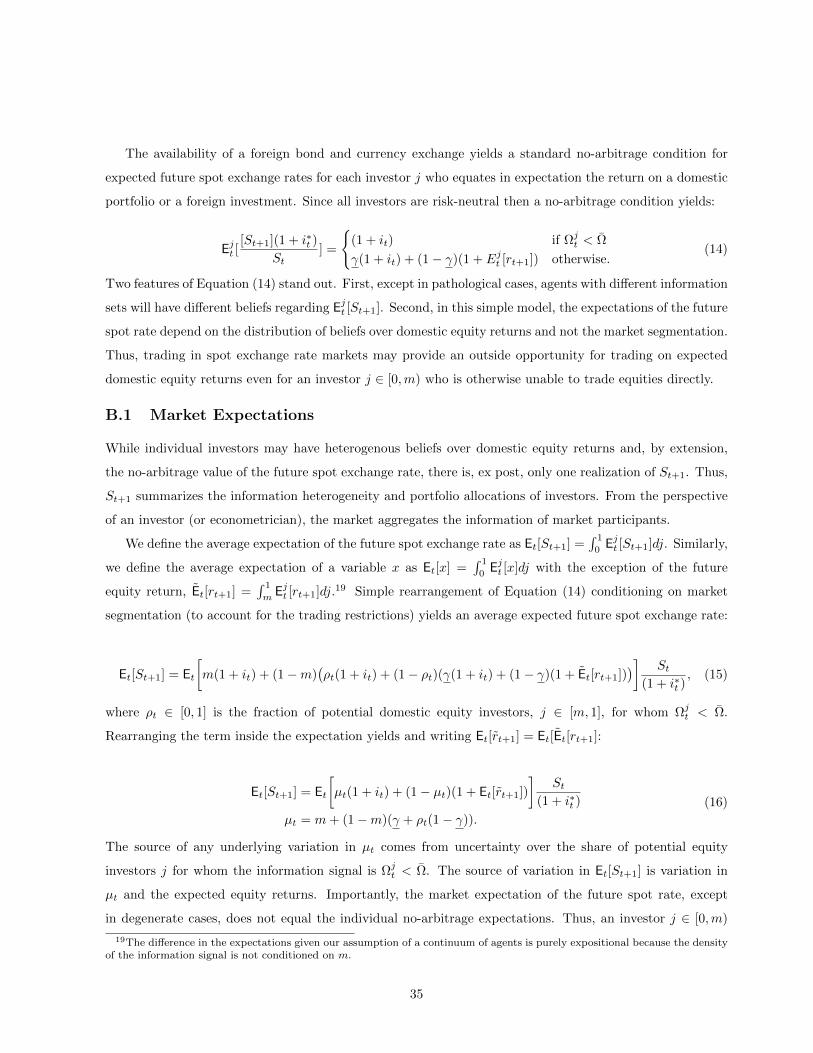
The availability of a foreign bond and currency exchange yields a standard no-arbitrage condition for

expected future spot exchange rates for each investor j who equates in expectation the return on a domestic

portfolio or a foreign investment. Since all investors are risk-neutral then a no-arbitrage condition yields:

Ejt [[St+1](1 + i∗t )

St] =

(1 + it) if Ωjt < Ω

γ(1 + it) + (1− γ)(1 + Ejt [rt+1]) otherwise.(14)

Two features of Equation (14) stand out. First, except in pathological cases, agents with different information

sets will have different beliefs regarding Ejt [St+1]. Second, in this simple model, the expectations of the future

spot rate depend on the distribution of beliefs over domestic equity returns and not the market segmentation.

Thus, trading in spot exchange rate markets may provide an outside opportunity for trading on expected

domestic equity returns even for an investor j ∈ [0,m) who is otherwise unable to trade equities directly.

B.1 Market Expectations

While individual investors may have heterogenous beliefs over domestic equity returns and, by extension,

the no-arbitrage value of the future spot exchange rate, there is, ex post, only one realization of St+1. Thus,

St+1 summarizes the information heterogeneity and portfolio allocations of investors. From the perspective

of an investor (or econometrician), the market aggregates the information of market participants.

We define the average expectation of the future spot exchange rate as Et[St+1] =∫ 1

0Ejt [St+1]dj. Similarly,

we define the average expectation of a variable x as Et[x] =∫ 1

0Ejt [x]dj with the exception of the future

equity return, Et[rt+1] =∫ 1

mEjt [rt+1]dj.19 Simple rearrangement of Equation (14) conditioning on market

segmentation (to account for the trading restrictions) yields an average expected future spot exchange rate:

Et[St+1] = Et

[m(1 + it) + (1−m)

(ρt(1 + it) + (1− ρt)(γ(1 + it) + (1− γ)(1 + Et[rt+1])

)] St(1 + i∗t )

, (15)

where ρt ∈ [0, 1] is the fraction of potential domestic equity investors, j ∈ [m, 1], for whom Ωjt < Ω.

Rearranging the term inside the expectation yields and writing Et[rt+1] = Et[Et[rt+1]:

Et[St+1] = Et

[µt(1 + it) + (1− µt)(1 + Et[rt+1])

]St

(1 + i∗t )

µt = m+ (1−m)(γ + ρt(1− γ)).

(16)

The source of any underlying variation in µt comes from uncertainty over the share of potential equity

investors j for whom the information signal is Ωjt < Ω. The source of variation in Et[St+1] is variation in

µt and the expected equity returns. Importantly, the market expectation of the future spot rate, except

in degenerate cases, does not equal the individual no-arbitrage expectations. Thus, an investor j ∈ [0,m)

19The difference in the expectations given our assumption of a continuum of agents is purely expositional because the densityof the information signal is not conditioned on m.

35

whose information yields an expectation of an excess equity return will prefer the RHS of Equation (14) as

Et[St+1] is greater than the no-arbitrage expected value of Ejt [St+1] given by Equation (14).

36