Unconventional Monetary Policy and the Allocation of Credit

∗

Marco Di Maggio

†Amir Kermani

‡Christopher Palmer

§

May 2016

Abstract

Despite massive large-scale asset purchases (LSAPs) by central banks around the world sincethe global financial crisis, there is a lack of empirical evidence on whether and how the compo-sition of purchased assets matters for the real effects of unconventional monetary policy. Usinguniquely rich mortgage-market data, we document that there is a “flypaper effect” of LSAPs,where the transmission of unconventional monetary policy to interest rates and (more impor-tantly) origination volumes depends crucially on the assets purchased and degree of segmenta-tion in the market. For example, QE1, which involved significant purchases of GSE-guaranteedmortgages, increased GSE-guaranteed mortgage originations significantly more than the origi-nation of non-GSE mortgages. In contrast, QE2’s focus on purchasing Treasuries did not havesuch differential effects. This de facto allocation of credit across mortgage market segments,combined with sharp bunching around GSE eligibility cutoffs, establishes an important com-plementarity between mortgage-market policy and the effectiveness of Fed MBS purchases. Inparticular, more relaxed GSE eligibility requirements would have resulted in more refinancingfrom economically distressed regions and fewer households deleveraging overall. Overall, our re-sults imply that central banks could most effectively provide unconventional monetary stimulusby supporting the origination of debt that would not be originated otherwise.

∗We thank our discussants, Florian Heider, Anil Kashyap, and Philipp Schnabl; Adam Ashcraft, Geert Bekaert,Charles Calomiris, Gabriel Chodorow-Reich, Andreas Fuster, Sam Hanson, Arvind Krishnamurthy, Michael Jo-hannes, David Romer, David Scharfstein, Jeremy Stein, Johannes Stroebel, Stijn Van Nieuwerburgh, Annette Vissing-Jørgensen, and Paul Willen; workshop participants at Berkeley and Columbia; and seminar participants at theCatholic University of Milan, the Econometric Society 2016 Meetings, Federal Reserve Board, HEC Paris, NBERMonetary Economics, Northwestern-Kellogg, NYU-Stern, NY Fed/NYU Stern Conference on Financial Intermedia-tion, Penn State, San Francisco Federal Reserve, Stanford, St. Louis Fed Monetary Policy and the Distribution ofIncome and Wealth Conference, University of Minnesota-Carlson, University of Illinois at Urbana-Champaign, andUSC-Price for helpful comments and discussions. We also thank Sam Hughes, Sanket Korgaonkar, Christopher Lako,and Jason Lee for excellent research assistance.

†Columbia Business School and NBER (mdimaggio@columbia.edu)‡University of California, Berkeley and NBER (kermani@berkeley.edu)§University of California, Berkeley (cjpalmer@berkeley.edu)

1

1 Introduction

In recent years, many central banks have undertaken unconventional monetary policy to stimulate

their economies, mainly through long-duration large-scale asset purchase programs (LSAPs). A

common feature of these programs is their significant size; the Federal Reserve increased the size

of its balance sheet more than fivefold (Figure 1). However, LSAPs have varied significantly in

the type of assets purchased by central banks, e.g., from Treasuries and Agency debt in the U.S.

to ETFs and corporate bonds in Japan. Despite the newfound popularity of LSAPs worldwide,

their effectiveness and the channels through which they affect the real economy have been at the

center of a vigorous policy and academic debate. We contribute to this debate by investigating the

channels through which LSAPs impact the real economy and ask whether the composition of assets

purchased (in addition to their duration) matters.1

There is no clear consensus on whether LSAPs do benefit an economy and on potential trans-

mission mechanisms. Non-standard open market operations are irrelevant in a frictionless world,

as shown by Wallace (1981) and Eggertsson and Woodford (2003). Moving away from a friction-

less world, the literature on unconventional monetary policy has suggested multiple explanations

for why LSAPs may have real effects. We highlight three of these pathways—see Krishnamurthy

and Vissing-Jorgensen (2011) for a comprehensive treatment of such channels along with empirical

evidence from asset yields on the relative importance of each. First, under the portfolio-balancing

channel, the central bank affects the return of different assets by affecting their relative supply.2

Second, the segmentation channel posits that LSAPs are effective when capital-constrained inter-

mediaries are unable to arbitrage in the short run across different market segments (e.g., Vayanos

and Vila, 2009 and Greenwood et al., 2015).3 Third, the capital-constraints channel highlights how

LSAPs can offset the decline in private lending from disruptions in financial intermediation (see

Gertler and Karadi, 2011 and Curdia and Woodford, 2011).

Under the portfolio-balancing and duration-segmentation channels, only the duration (or riski-

1As discussed below, this “what you buy matters” point was first made by Krishnamurthy and Vissing-Jorgensen(2011) using asset prices and credit spreads.

2LSAPs could have real effects by taking safe assets out of the market and therefore inducing cautious investorsto take more risk. For related arguments, see Gurley et al. (1960), Tobin and Brainard (1963), Tobin (1969), andBrunner et al. (1973).

3We refer to this channel as the duration-segmentation channel if the inhibiting segmentation is along assetduration.

2

ness) of assets purchased drives their effectiveness because investors will reallocate their resources to

other similar assets not purchased by the central bank. However, if investors specialize in trading a

specific asset class, or if the financial intermediation sector is constrained, there will be only limited

spillovers of central-bank purchases to other asset classes, and the effectiveness and allocative ef-

fects of LSAPs will depend on not only the duration but also the specific type of assets purchased.4

In other words, to the extent that portfolio rebalancing or duration-segmentation is driving the

effectiveness of LSAPs, we should observe spillovers from central-bank purchases to other assets

with similar duration. An absence of such spillovers would support the view that LSAPs stimulate

real activity through the capital constraints channel or a narrow-segmentation channel. This paper

empirically investigates this hypothesis.

Identifying the effects of aggregate policies is particularly challenging given that such policies

explicitly respond to current and anticipated aggregate shocks. For traction, most of the litera-

ture has used event studies of short-run asset-price changes immediately surrounding central bank

policy announcements. We supplement such before/after comparisons with an identification strat-

egy that exploits the segmentation of the U.S. mortgage market and the legal restriction that the

Fed can only purchase mortgages guaranteed by the Government Sponsored Enterprises (GSEs).

The outstanding balance on GSE-guaranteed mortgages must be less than the so-called conforming

loan limits and must have loan-to-value ratios at or below 80 percent.5 This allows us to estimate

the effects of quantitative easing by contrasting how each LSAP campaign affected refinancing ac-

tivities in the conforming and non-conforming segments. Specifically, finding spillovers between

these two segments supports the portfolio-rebalancing channel or duration-segmentation channels

of unconventional monetary policy, while rejecting spillovers would be more consistent with the

capital-constraints or narrow segmentation channels.

We start our analysis by considering the changes in mortgage interest rates. Consistent with

existing work, we find that interest rates decreased by more than 100 basis points on average in

response to the beginning of QE1. However, we show that interest rates on jumbo loans decreased

significantly less, increasing the jumbo-conforming spread by 40-50 basis points, nearly as much as

this spread increased from the collapse in private securitization in late 2007. By contrast, QE2,

4Agency-mortgage REITs are one example of such an investor, investing mainly in a single asset class.5An important exception to the 80% LTV cutoff was made possible by the Home Affordable Refinancing Program

(HARP), a policy we show had visible effects on the effectiveness of Fed MBS purchases.

3

the Maturity Extension Program (“Operation Twist”) enacted in September 2011, and QE3 led to

overall mortgage rate reductions of 20-40 basis points without detectable differential effects across

conforming and non-conforming segments. We also investigate the effects of the Fed’s tapering its

MBS purchases starting in June 2013, finding that rates increased in response by about 25 basis

points more for the conforming segment than the non-conforming segment.

We then turn to examining the main question of the paper, how unconventional monetary

policy affected the volume of new mortgages issued. We find that financial institutions more than

tripled their monthly origination of mortgages that were eligible for purchase by the Fed around the

announcement of QE1, while the origination of loans above the conforming loan limits increased

much less dramatically. Next, we verify that this heterogeneity in the mortgage market response

to QE1 was a function of the type of debt the central bank purchased, by contrasting the effect

of various QE episodes. As shown in Figure 3 and discussed in detail in Section 3, QE1 and QE3

involved MBS and Treasury purchases, while QE2 purchases consisted exclusively of Treasuries.

We show that MBS purchases had a relatively immediate and economically significant effect on

refinancing activity. QE1 in particular, which occurred at a time when the banking sector was

much less healthy than in QE3, had a much stronger impact on the origination of mortgages that

were eligible to be bundled into the type of MBS that the Fed was purchasing, with more modest

effects on other types of mortgages.

Our focus on quantities has several advantages over studies that rely on high-frequency asset-

price event studies. Asset prices respond immediately to central bank announcements, making it

unlikely that other shocks hit market prices at the same time as QE announcements. However, mar-

ket price reactions in the immediate short run might be very different from the programs’ effects

in the longer run.6 Second, event-study papers investigate secondary-market yields.7 To the extent

that the pass-through of mortgage-backed securities (MBS) yields to primary-market mortgage in-

terest rates is imperfect during this period (as documented in Fuster et al., 2013 and Scharfstein and

Sunderam, 2013), these studies may overstate the real effect of LSAPs. More importantly, interest

rates are observed conditional on origination, meaning that inferring the effects of unconventional

monetary policy by merely looking at interest rate changes will be an overstatement by assuming

6This can be either because of partial segmentation of different asset classes as in Greenwood et al. (2015) orbecause investors’ understanding of the effectiveness of LSAPs changes over time.

7A notable exception is Hancock and Passmore (2011), who look for effects on primary-market mortgage rates.

4

perfect availability of credit.8 These reasons motivate our focus on the detection of “real effects” of

unconventional monetary policy, specifically of the credit easing induced by LSAPs as distinct from

effects on financial variables like asset prices and interest rates.

To identify the causal impacts of LSAPs, we account for time-varying credit demand and supply

shocks that might otherwise confound our results. First, our loan-level dataset combines agency

and non-agency mortgages, allowing us, for example, to compare observationally similar loans above

and below the conforming loan limit that are plausibly exposed to the same shocks to funding

and fundamentals. Event studies support this parallel trends assumption, particularly with our

specifications’ tight windows around policy dates. Further steps to address demand shocks include

focusing on refinancing, which is mainly driven by changes in interest rates, and controlling for

regional shocks to fundamentals (income, house prices, expectations, etc.) by controlling for county

⇥ month effects. Additional measures suggest that our results are not driven by segment-specific

credit supply shocks. We focus our analysis on the post-2008 period to avoid making inference off of

the asset-backed securities market disruptions that differentially affected the jumbo-lending market

as it transitioned away from being heavily reliant on private securitization (Chernenko, Hanson, and

Sunderam, 2014). We also show that our results are robust to the inclusion of time-series controls

proxying for segment-specific shocks to funding availability (BBB-AAA credit spreads and GSE

guarantee fee changes).

Finally, we complement this mortgage-level evidence with borrower-level evidence using a novel

dataset linking mortgages to borrowers and their credit bureau information to track borrowers be-

fore and after they take out a new mortgage to study how households responded to the differential

improvement of the GSE-eligible segment of the mortgage market. Theoretically, refinancing can

affect consumption through three different channels. First, savings from lower monthly payments

result in immediately higher disposable income (Di Maggio et al., 2014 and Keys et al., 2014).

Second, the present value of lower interest payments functions as a positive (albeit illiquid) wealth

shock for borrowers even absent any change in monthly payments. While both these channels sup-

port increased consumption by refinancers, a third channel might amplify or mitigate the strength

8The preponderance of fixed-rate mortgages in the United States means that most households need to qualifyfor a new refinance mortgage to benefit from monetary stimulus, excluding underwater fixed-rate borrowers (andfixed-rate borrowers who cannot qualify for new refinance mortgages) from the direct benefits of QE (see Di Maggioet al., 2014 and Keys et al., 2014 for further discussion).

5

of such a response in aggregate. When borrowers have insufficient equity to refinance, they may

cash-in refinance by bringing cash to closing to take out a smaller loan than their previous one,

decreasing their stock of liquid wealth. Conversely, borrowers with sufficient equity may choose to

cash-out refinance, with the opposite implication for cash-on-hand and with likely very different

impacts on consumption (Kaplan and Violante, 2014 and Greenwald, 2016). This effect is indeed

very sizable; we find that over 40% of jumbo borrowers who refinanced from 2008–2013 took out a

GSE-eligible loan, on average paying down their original mortgages by $81,000. A similar fraction of

borrowers who refinance loans with current LTVs over 80 percent engage in cash-in refinancing, on

average paying down $12,300 of mortgage principal. Importantly, we also find that the Home Afford-

able Refinancing Program (HARP) alleviated this deleveraging behavior significantly by allowing

eligible high-LTV borrowers refinancing opportunities, highlighting the complementarity between

unconventional monetary policy and other interventions in the mortgage market.

Overall, the targeted nature of the Fed’s MBS purchase program coupled with its lack of spillovers

during QE1 means that Fed purchases de facto allocated credit within the mortgage market towards

GSE-eligible borrowers, complementing the results on bond yields and credit spreads in Krishna-

murthy and Vissing-Jørgensen (2011, 2013). An immediate implication of this lack of reallocation

is that the borrowers who benefitted the most from monetary stimulus during the recession had rel-

atively high levels of home equity or cash-on-hand and disproportionately lived in the least hard-hit

areas.

The paper proceeds as follows. Section (2) reviews the relevant academic literature on monetary

policy transmission. Section 3 provides further background on the Federal Reserve’s Quantitative

Easing program as well as institutional details about the credit markets we study in this paper.

Sections 4 and 5 detail the data sources used in our analysis and our research design, respectively.

Section 6 presents our results on debt origination and household behavior, and section 7 summarizes

and concludes with a discussion of policy implications.

2 Related Literature

The main contribution of the paper is to provide evidence that the Fed de facto allocated credit

through LSAPs and to show that these programs had very limited spillovers to other assets. It con-

6

tributes to the empirical literature on LSAPs which generally finds that targeted asset purchases

and/or direct extensions of credit to private borrowers by the Fed and other central banks have

affected equilibrium rates of return, including Ashcraft et al. (2011), Baba et al. (2006), Gagnon et

al. (2010), Hancock and Passmore (2011), Sarkar and Shrader (2010), Stroebel and Taylor (2012)

and Swanson (2015).9 The key studies we build on are Krishnamurthy and Vissing-Jorgensen (2011,

2013), who illustrate that there is important heterogeneity across asset classes in terms of which

yield curves are the most affected by LSAPs. Their conclusions are consistent with the view that

LSAPs bid up bond prices (pushing yields lower) by shifting outward the demand for debt, with

the implication being that this movement along the supply curve should result in additional debt

issuance proportional to the effect on the price of debt (interest rates). Under this transmission

mechanism, whether LSAPs induce a significant change in the yield curve measures policy effec-

tiveness. In addition to providing corroborating evidence on the effects of QE on asset returns as

highlighted by these papers, we complement this literature by documenting how LSAPs shaped the

refinancing activities in the aftermath of the crisis and induced households to delever to be able to

refinance their debt.

Our results also inform the growing theoretical literature studying the effects of unconventional

monetary policy. Until the financial crisis, the benchmark theory for many macroeconomists has

always been that non-standard open market operations in private assets are irrelevant as shown first

by Wallace (1981), and extended to models with nominal frictions, money in the utility function

and zero nominal interest rate by Eggertsson and Woodford (2003). The idea in these papers is that

once the nominal interest rate reaches its lower bound, liquidity has no further role in this class of

models, or in most other standard models with various types of frictions, such as Rotemberg and

Woodford (1997) or Christiano et al. (2005).

In the aftermath of the crisis, other studies have highlighted the mechanisms through which

unconventional monetary policy can have a significant impact. For instance, Curdia and Woodford

(2011) provide a model with heterogeneous agents and imperfections in private financial intermedi-

ation to demonstrate that quantitative easing will affect the economy provided either 1) the increase

in reserves increases central-bank lending to the private sector or 2) the policy changes expecta-

9See also Chodorow-Reich (2014) and Di Maggio and Kacperczyk (2015), who study the impact of unconventionalmonetary policy on different sectors of the financial markets, such as pension funds, insurance companies, and moneymarket funds.

7

tions about how future interest-rate policy will be conducted, both of which seem to be satisfied by

QE1. Brunnermeier and Sannikov (2015) show that monetary policy can work against the adverse

feedback loops that precipitate crises by affecting the prices of assets held by constrained agents

and redistributing wealth. Drechsler et al. (2014) point out the role played by large-scale asset pur-

chases, equity injections, and asset guarantees in supporting risky asset prices. Similarly, Gertler

and Karadi (2011) show in the context of a DSGE model of unconventional monetary policy that

during a crisis, the balance sheet constraints on private intermediaries tighten, raising the net bene-

fits from central bank intermediation. These benefits may be substantial when the zero lower bound

constraint binds. Greenwood et al. (2015) demonstrate that understanding market segmentation is

important in designing and evaluating LSAPs.

Closer in spirit to our analysis is the work by Del Negro et al. (2011), who investigate the

effects of interventions in which the government provides liquidity in exchange for illiquid private

paper once the nominal interest rate reaches the zero bound. In their study, the source of the 2008

crisis is a shock to the liquidity of private paper (e.g., mortgage-backed securities) with secondary

markets for these securities freezing. They show that unconventional monetary policy can alleviate

the crisis by directly targeting the source of the problem, which is the illiquidity of private paper.

By swapping illiquid private paper for liquid government debt, the Fed improves the liquidity of the

aggregate portfolio holdings of the private sector, and the intervention lubricates financial markets,

arresting the fall in investment and consumption. We test this mechanism and show that the type

of purchases made by the Fed matter for understanding the response of the financial institutions.

That is, injecting liquidity by purchasing MBS has a different effect than purchasing Treasuries.

Our paper is also related to a broader strand of the literature that investigates the channels

through which monetary policy impacts banks’ lending decisions. In a seminal paper, Kashyap and

Stein (2000) provide evidence of the bank lending channel of the transmission of (conventional)

monetary policy. More recently, Jimenez et al. (2014) show that a lower overnight interest rate

induces less capitalized banks to lend to riskier firms, while Jimenez et al. (2012) show that for

distressed banks, tighter monetary policy and worse economic conditions substantially reduce lend-

ing. Agarwal et al. (2015) estimate banks’ marginal propensity to lend out of a decrease in their

cost of funds to show that banks were reluctant to lend to riskier borrowers in the aftermath of the

crisis. Maddaloni and Peydro (2011) find that low short-term interest rates for an extended period

8

eventually soften lending standards for household and corporate loans.10 Finally, Rodnyansky and

Darmouni (2016) look explicitly at the effect of QE on bank lending, finding MBS purchases to

have important implications for which banks are able to increase credit supply in response to QE3.

We add to these studies by uncovering the impact of unconventional monetary policy on individual

household refinancing, deleveraging, and consumption decisions.

Finally, we also contribute the literature investigating the redistributional consequences of mon-

etary policy, e.g., Doepke and Schneider (2006), Fuster and Willen (2010), Coibion et al. (2012),

Sterk and Tenreyro (2014). Particularly related to our study is Beraja et al. (2015), who use

borrower-linked refinance data to show that the heterogeneous regional effects of QE1 covary with

regional economic conditions and amplify existing regional disparities.

3 Background

In this section, we provide a brief summary of the Federal Reserve’s Quantitative Easing program

and discuss how its MBS purchases were conducted on the secondary mortgage market. For ref-

erence, Figure 2 provides a timeline of the various Fed LSAP programs.11 QE1 lasted from late

November 2008 until March 2010, and QE2 was first announced in mid-August 2010 and ran from

November 2010 to June 2011. In September of 2011, the Fed began a program known as the Matu-

rity Extension Program (MEP) or Operation Twist. We consider QE2 to have begun in September

2010 when the Fed signaled that it was considering a second round of monetary stimulus and June

2013 for the beginning of the Fed tapering, following Bernanke’s tapering announcement on May 22,

2013.12 Under the MEP, the Federal Reserve reduced the supply of longer-term Treasury securities

in the market by selling and redeeming about $600 billion in shorter-term Treasury securities and

using the proceeds to buy longer-term Treasuries.13 QE3 was announced in September 2012.

In late November 2008, the Fed announced its mortgage-buying program with the intent to

10See also Bernanke and Blinder (1988), Christiano and Eichenbaum (1992), Landier et al. (2013), Stein (2012)and Williamson (2012).

11As detailed in Appendix Table 1, where possible, we have relied on the dates provided by Krishnamurthy andVissing-Jorgensen (2013).

12Krishnamurthy and Vissing-Jorgensen (2013) found that most of the market reaction to QE2 was when it wasfirst signaled in September 2010. Interest rates actually increased after the official announcement in November 2010as it failed to live up to market expectations.

13See Foley-Fisher, Ramcharan, and Yu (2014) for a recent paper on the effect of this program on firms’ financingconstraints.

9

purchase about $500 billion in mortgage-backed securities, consisting of mortgages guaranteed by

Fannie Mae, Freddie Mac, and to a lesser extent, Ginnie Mae. In March 2009, the Fed announced an

expansion to this program, subsequently purchasing an additional $750 billion in mortgage-backed

securities with 50-70% Agency originations each month ending up on the Fed’s balance sheet. The

first quantitative easing program ended in the first quarter of 2010, with a total of $1.25 trillion in

purchases of mortgage-backed securities and $175 billion of agency debt purchases. Figure 3 depicts

the gross amount of MBS purchased and sold by the Fed since beginning LSAPs. During QE1, the

Fed purchased both MBS and Treasuries with a greater emphasis on MBS purchases. QE2, on the

other hand, was exclusively focused on Treasuries, and QE3 was roughly equally weighted between

Treasuries and MBS. As Figure 3 shows, a greater fraction of each QE campaign’s MBS purchases

have occurred at the beginning of each program, with purchases slowly declining over the course

of each LSAP campaign.14 Notably, the Fed was effectively able to purchase $1.85 trillion (about

40% more than the usually reported $1.25 trillion amount of net purchases) by contemporaneously

reselling a substantial fraction of these securities, perhaps enhancing market liquidity without further

expanding the Fed balance sheet. Figure 4 shows the relative magnitude of GSE MBS net purchases

compared with the total size of the GSE-guaranteed mortgage market. During QE1, the volume of

Fed purchases was similar in magnitude to the volume of new issuance of GSE-guaranteed MBS.

During QE3, Fed net GSE MBS purchases were roughly half of the GSE market.

Contrary to popular perception, Fed MBS purchases did not involve buying legacy (and under-

performing) MBS from banks. Instead, Fed MBS purchases were on the TBA (To-be Announced)

mortgage market.15 A key feature of the Agency MBS market is the existence of this highly liquid

forward market, through which more than 90% of Agency MBS trading volume occurs and which

consists predominantly of newly originated mortgages (Vickery and Wright, 2013), with trading

volumes on the order of $200 billion per day and around $100 billion delivered each month. See

Appendix A for additional details on the TBA market.

Nevertheless, the eligibility requirements for mortgages to be included in TBAs provide to sharp

14Note that the policy of the Fed to reinvest principal prepaid on its MBS holdings into new MBS purchases resultsin non-zero MBS purchases even after QE3 officially ends.

15A limited number of the TBA securities purchased by the Fed at the beginning of QE1 included MBS CUSIPsthat had been originated in early 2008 instead of roughly contemporaneous with Fed purchases. Still, these wereGSE-eligible mortgages originated in 2008 and not the types of legacy MBS that were troubling banks, having beenfilled with mortgages originated under questionable underwriting standards that were deeply underwater by 2009.

10

cross-sectional predictions on the effect of MBS purchases on loan originations. Because TBA

delivery must be accomplished with Agency-eligible mortgages that are usually recent originations,

the strict eligibility rules for GSE guarantees allow us to compare origination volumes by loan

size. Specifically, GSE guarantees require loan sizes to be beneath published conforming loan limits

(CLLs).16 Mortgages with a loan size exceeding geographically and time-varying CLLs (known as

jumbo mortgages) are essentially ineligible for inclusion in GSE MBS. Many of our results below

will test for a deviation in mortgage origination volume for loans just below the CLL, which should

be directly affected by Fed purchases because of their TBA eligibility, and loans just above the CLL,

which should only be indirectly affected by Fed MBS purchases.

4 Data

The workhorse data source we use is the Equifax’s Credit Risk Insight™ Servicing McDash (CRISM)

dataset, which covers roughly 65 percent of the mortgage market during our sample period (2008-

2013), first used to examine the effects of QE by Beraja (2015). One of the features of this dataset is

that it merges McDash Analytics mortgage-servicing records (from Lender Processing Services) with

credit bureau data (from Equifax). This provides us with information about the characteristics of

each mortgage at origination, such as the mortgage type, the size of the loan, the monthly payments,

the interest rate, the borrower’s FICO, as well as their behavior over time. In addition, we also

observe all the other liabilities of the borrowers, such as their auto loans, HELOCs, and credit

cards.Panels I and II of Table 1 report loan-level summary statistics on conforming and jumbo

loans from the CRISM database. Our sample include more than seven million loans below the

conforming loan limit and about 170,000 jumbo loans. On average, non-jumbo (jumbo) borrowers

in our sample have a 750 (760) FICO score and an LTV of 67% (65%). The average balance of

conforming and jumbo loans in our data are $211,000 and $960,000, respectively. Panel III reports

summary statistics for time series controls used in robustness checks, including guarantee fees from

Fuster et al. (2013) and bond yields from Federal Reserve Economic Data (FRED) at the Federal

Reserve Bank of St. Louis. The guarantor fees are about 34 basis points, while the BBB-AAA bond

spread is about 134 basis points over our sample period.16See Adelino et al. (2013) and DeFusco and Paciorek (2015) for studies of the consequences of the sharp change

in GSE eligibility at the conforming loan limit.

11

The unique advantage of this data is that it enables us to link multiple loans by the same borrower

together, allowing us to gather more complete information about the circumstances accompanying

a borrower’s refinancing decision. While existing datasets follow individual mortgages over time, we

can match borrowers to mortgages and observe each borrower in the credit bureau data six months

before any mortgage origination and track him as the current mortgage is refinanced. Appendix

Table 2 demonstrates the usefulness of this linkage, reporting a refinancing transition matrix of

mortgage product types for each year from 2006–2013. This dimension of the dataset (linking

refinance mortgages to prior mortgages) allows us to study cash-in/cash-out refinancing much more

accurately. For example, by observing the outstanding amount of the old loan and the principal

amount of the new loan, we can measure the dollar amount of equity that is added to the borrower’s

position during the refinancing process.

5 Empirical Strategy

In this section we present our main empirical strategy to identify the effects of LSAPs on both

interest rates and refinancing volumes.

5.1 Quantifying the Effect of QE on Interest Rates

In the spirit of the empirical QE literature’s focus on debt yields, we begin by comparing the

reaction of the interest rates to LSAPs for loans above and below the conforming loan limit. To

form a comparable jumbo/conforming sample, we only consider loans that are 30-year fixed-rate

first-lien mortgages secured by owner-occupied single-family houses with an initial LTV of 25-80%

and without any prepayment penalty or balloon-payment or interest-only deferred amortization

features.17 We also drop FHA mortgages, which require mortgage insurance and have more flexible

lending requirements than those for conventional loans.

Changes in borrower composition over time limit the usefulness of simple time-series comparisons

of interest-rates. Instead, we take into account that rates change in response to changing mortgage-

borrower characteristics. For example, some of the decrease interest rates that we observe is due

17Appendix Table 2 shows that a third of all refinance mortgages are transitions from one 30-year fixed-ratemortgage to another.

12

to stricter credit standards at the end of our sample—later mortgages feature both higher average

FICO scores and lower LTVs.

To facilitate graphical comparisons of composition-adjusted interest rates over time, we estimate

the following regression separately for loans above and below the conforming loan limit

rit

= ↵t

+ �1(FICOi

� 720) + �2(LTVi

� 0.75) + "it

,

where rit

is the interest rate of loan i at time t measured in basis points. We control for the

difference between the FICO score and loan-to-value ratio of loan i and benchmark FICO and LTV

ratios such that estimated time effects ↵t

capture “rate-sheet–adjusted” interest rates—interest rates

for a representative borrower with a FICO score of 720 and an LTV ratio of 75%.

To quantity the differential reaction of jumbo and conforming interest rates to purchase program

events, we pool jumbo and non-jumbo mortgages together and estimate the following loan-level

specification around the beginning of each monetary policy event separately

rict

= X 0i

� + ✓1Programt

+ ✓2Programt

· Jumboi

+ �ct

+ "ict

(1)

where Program is an indicator for month t being after the institution of a specific monetary policy

program (e.g., QE1), Jumboi

is an indicator variable for whether loan i was a jumbo mortgage,

and Xi

is a vector of flexible loan-level controls consisting of 5-point LTV bins, 20-point FICO bins,

and an indicator for missing FICO scores. We also control for county ⇥ month fixed effects �ct

to

purge interest rates in both segments of static and time-varying regional shocks to credit demand,

including differences in house price growth. We consider the three quantitative easing programs as

well as the Maturity Extension Program in September 2011 and the beginning of tapering in June

2013. We choose to cluster our standard errors at the month level to account for the correlation

between contemporaneous shocks across loans and geographies.

The coefficient ✓1 reports the number of basis points by which interest rates for non-jumbo

mortgages fell on average in the three (or six) months immediately following the beginning of each

QE campaign relative to the period immediately prior. The coefficient ✓2 tells us how the jumbo-

conforming spread changed in response to each QE campaign’s commencement, in other words by

how much more or less interest rates in the jumbo segment responded. We interpret ✓1 as causal only

with some degree of caution because it will combine the effect of LSAPs with any contemporaneous

13

shock to mortgage rates, even those effects not caused by the monetary policy events in question.

The identifying assumption behind our causal interpretation of ✓2 is that, conditional on borrower

and loan characteristics and county-month fixed effects, time-varying shocks do not affect the jumbo

and conforming differently. In other words, our ability to identify the effect of unconventional

monetary policy on mortgage-market segments relies on a parallel-trends assumption, which, as

we discuss below, seems to be satisfied, especially over the short time horizons used to estimate

equation (1).

5.2 Quantifying the Effect of QE on Mortgage Origination Volumes

As discussed above, inferring the impact of unconventional monetary policy from changes in the

interest rates tends to overstate policy effectiveness by assuming perfect availability of credit. In

particular, interest rates are observed conditional on origination, but not all mortgages are eligible

for purchase by the Fed. Considering the volume of debt issuance in response to the LSAPs is an

essential consideration in estimating the response of financial markets to new measures of monetary

policy adopted after the crisis. Furthermore, we can test for the presence of spillovers from the

conforming segment, directly affected by the LSAPs, to the jumbo segment.

To form a comparable jumbo/conforming sample, we drop FHA mortgages and consider first-lien

refinance loans for single-family houses (note that this sample restriction is more inclusive than the

interest-rate sample restrictions needed to compare interest rates on equal footing). We quantify

these effects on origination volumes Qsct

at the county c ⇥ month t ⇥ mortgage-market segment

s 2 {Jumbo, non-Jumbo} level by estimating

logQsct

= �1Programt

+ �2Programt

· Jumbos

+ �X 0t

· Jumbos

+ ↵ct

+ "sct

. (2)

For each policy event, we provide baseline results and subsequent robustness checks containing

a more restrictive specification in which we interact time-varying aggregate factors Xt

that may

differentially affect each segment with a the segment indicator Jumbos

and allow for county ⇥

month fixed effects ↵ct

. We also restrict attention to counties where we observe an active jumbo

market by restricting the sample to counties that have at least one jumbo refinance origination each

month. Again, we conservatively cluster our standard errors at the month level.

The coefficient �1 tells us by how many log points average county ⇥ segment origination volumes

14

increased in the months following an LSAP event relative to the months immediately preceding that

event. We focus our attention on �2, which is an estimate of whether jumbo origination volumes

responded differently from conforming origination volumes. Again, the identifying assumption re-

quired for �2 to be an unbiased estimate of differential allocation of LSAP credit across mortgage

market segments is that there were no other shocks occurring coincident with QE events that af-

fected the jumbo market more (or less) than the conforming market. The requirement for parallel

trends across conforming and non-conforming segments justifies our focus on the conforming loan

limit since underwriting standards in the conforming and prime jumbo market are similar. The

graphical evidence discussed below also supports this parallel-trends assumption.

5.3 Estimating Changes in the Propensity to Refinance

A complementary way to examine the impact of QE uses the individual-level panel structure of our

data to test whether each QE campaign altered the likelihood that a given individual refinanced.

Analyzing how individual access to refinancing changed during QE1 with respect to characteristics

of the original mortgage is an input into understanding how credit might have been allocated in

counterfactual scenarios with, for example, higher GSE LTV caps. We estimate a hazard model of

the form

�it

= exp(X 0it

�)�0(t� t0(i))

X 0it

� = ✓0L

W loan

it

+ ✓0B

W borrower

i

+

X

k

Feb2008X

⌧=Dec2008

�k⌧

·QE1

t

⇥ Sk,it

where �it

is the instantaneous probability that loan i will refinance in the calendar month corre-

sponding to loan-age t, conditional on not yet having refinanced by month t. The nonparametrically

estimated baseline hazard function �0(·) is a function of loan age (current month t minus loan i’s

origination month t0(i)) and captures the standard life-cycle of mortgage prepayment, while covari-

ates scale the baseline hazard depending on their contribution to prepayment risk. The covariates

in Xit

consist of loan- and borrower-level controls. Loan-level controls W loan

it

include current LTV,

original balance, and an indicator for whether the loan size is currently above the conforming loan

limit. Borrower-level controls W borrower

it

include FICO bins, DTI ratio, and an indicator for whether

the DTI is missing. The coefficients of interest are �k⌧

, which are coefficients for each of the three

15

months following the beginning of QE1 on the QE1 indicator variable interacted with two separate

indicators for whether loan i is currently GSE ineligible (whether loan i’s current LTV exceeds .9

and whether its loan size exceeds the CLL). We take for our sample all loans that were outstand-

ing as of September 2008, and use the continuous-time maximum-likelihood estimator described in

Palmer (2015). Estimated coefficients report partial effects on the log refinancing hazard. We limit

the sample to fixed-rate first-liens secured by owner-occupied single-family homes originated before

January 2008 and outstanding as of January 2008.

6 Results

We present three main sets of results. First, we examine the response of mortgage rates to the

LSAPs, we then turn to the changes in refinancing volume in the mortgage market. Finally, we turn

to the household-level analysis to shed further lights on how LSAPs affected households’ refinancing

decisions.

6.1 The Effect of LSAPs on the Primary Mortgage Market

6.1.1 Interest Rate Results

In Figure 5, we plot the estimated interest rates for loans above and below the conforming loan

limit. There is a visible change in interest rates as QE1 began, when mortgage interest rates declined

markedly, from 6.5% to about 5.5% and 5% for loans just above and just below the conforming loan

limit, respectively. While rates for the two types of loans follow each other quite closely, conforming-

loan rates declined almost 50% more than prime jumbo mortgage rates. For context, the increase

in the jumbo-conforming spread from the announcement of QE1 is on par with the spread increase

observed in the second half of 2007, when the securitization market froze.

To quantify the average magnitude of these effects over each monetary policy event, Tables 2 and

3 report the estimates for the interest-rate response to the announcements of the different LSAPs

within a three-month window (Table 2) and a six-month window (Table 3) around the event, both

for jumbo and non-jumbo loans. We find that the most significant reaction is to the announcement

of QE1 with an interest-rate reduction of more than 100 basis points. Consistent with Figure 6,

jumbo-mortgage interest rates also decline after QE1, but the conforming rate falls by an additional

16

40 basis points. Interestingly, rates decline by 35 basis points in response to QE2, without any

differential effect across segments, which is suggestive of the fact that the Fed was purchasing only

Treasuries during that program. This lower reduction in interest rates might also be indicative

that, while QE1 was a significant surprise, the second quantitative easing program was largely

anticipated by market participants. The maturity extension program also resulted in a reduction of

about 40 basis points, but we observe no differential effect for the conforming and non-conforming

segments. QE3, instead, led to a reduction of about 20 basis points in the three months after the

beginning of the program. Finally, the beginning of the Fed tapering led to an increase in interest

rates concentrated in the conforming loan segment. The results are qualitatively similar when we

consider a longer window around the announcement in Table 3, but their economic magnitude is

significantly larger.

Our identification approach is particularly suited to control demand shocks affecting both seg-

ments at the same time. In each specification we control for loan characteristics, including flexibly

specified loan-to-value ratios and FICO scores, to ensure that the differential response of jumbo and

conforming mortgages is not driven by time-varying borrower composition. In columns 2, 4, 6 and

10 of Tables 2 and 3, we absorb time-varying regional heterogeneity and find that our results on the

jumbo-conforming spread are not driven by such shocks.

Overall, these results show two robust patterns. First, interest rates decline significantly more for

the conforming market during QE1, which indicates that mortgage market segmentation crucially

affected its response to Fed purchases. Second, the interest rate decline is strongest for QE1, while

we detect little effect for QE2, which suggests that the type of assets purchased by the Fed (MBS

vs. Treasuries) plays a key role in determining the effectiveness of these measures.

6.1.2 Mortgage Origination Results

Figure 6 plots the origination amount of refinance mortgages recorded by LPS for mortgages with

loan sizes above and below the GSE conforming loan limit (CLL). The jumbo and non-jumbo

segments trend very similarly in origination counts and total volume prior to the beginning of QE1,

bolstering our identifying assumption of parallel trends. Right at the commencement of QE1, the

amount of refinance origination increases by a factor of three (counts) or four (dollar volume). The

sudden increase and subsequent fading of below-CLL refinance originations coincides quite closely

17

with the dynamics of Fed MBS purchases, as seen in Figure 7. By contrast, refinance origination

above the conforming loan limit is fairly flat until a modest increase in April 2009. In other words,

while the increase in the conforming spread indicates a differential response of rates depending on

GSE eligibility, loan origination suggests an even deeper relationship between the allocation of credit

supply and QE1 MBS purchases.

Table 4 reports results from estimating equation (2) for a three-month window (panel I) and

a six-month window (panel II).18 The dependent variable is the log of the total dollar amount

of monthly loan origination. Focusing on the conservative three-month window specification in

panel I, column 1 of Table 4 show that overall mortgage refinancing activity increased by 100

log points (170%) during QE1, with almost all of the effect concentrated in the conforming loan

segment. In contrast, during both QE2 and the MEP, both conforming and jumbo originations

increased by about 65% (50 log points), without no detectable differential effect across loan segments.

Column 4 shows that mortgage refinancing volumes responded very similarly across segments in

the months immediately following the beginning of QE3, increasing by 15-30%. Finally, refinancing

activities in the conforming segment fell significantly (30-50%) in the aftermath of the Fed’s tapering

announcement. Note that the total effect of tapering on jumbo originations in column 5 of Table 4

is close to zero, suggesting that jumbo originations were relatively unaffected by the tapering.

In sum, Fed asset purchases were effective at inducing new debt origination and cheaper monthly

payments for households. Purchasing mortgage-backed securities was particularly important during

QE1, when monetary stimulus was needed the most and LSAP spillovers were limited. More broadly,

the evidence suggests that loan origination is a more revealing indicator of de facto allocation of

credit by Fed purchases.

6.1.3 Robustness to Allowing for Correlated Time-Varying Shocks

Our identification strategy takes advantage of the natural segmentation in the mortgage market and

effectively employs a differences-in-differences approach in an event-study framework by comparing

the refinancing activities in the conforming (the treated group) and non-conforming (the control

18As discussed in section 5, our identifying assumption (and robustness checks below) of no mortgage segment-specific shocks allows us to interpret the coefficient on the program ⇥ jumbo indicator as reflective of the differentialimpact of each LSAP program on origination volumes. We acknowledge, however, that contemporaneous aggregateshocks can confound our estimates of the main effect of each LSAP event.

18

group) segment in a narrow window around the policy events. This allows us to limit the role of other

common shocks affecting both segments at the same time and control for changes in credit demand.

However, one potential limitation of this approach is the possibility that unobserved credit supply

shocks, occurring at about the same time of the policy announcements and differentially impacting

the conforming and jumbo loan segments, might confound our results. For example, because jumbo

mortgage investors bear default risk that GSE mortgage investors do not, lenders might face different

shocks to funding constraints in the two segments of the market.

We propose two such shocks (credit-spread shocks and guarantee fees), demonstrate that they

explain a significant amount of variation in differential movements in the jumbo and conforming

segments, and verify that our r results are robust to the inclusion of time-series controls measuring

aggregate shocks to funding availability in these two segments. The BBB-AAA bond spread and

the guarantee fee (“g-fee”) originators must pay to the GSEs to accept a loan’s default risk together

explain 70% of the variation in the jumbo-conforming spread. Intuitively, the credit spread captures

the price of risk and the g-fee reflects the price to avoid default risk, both of which might influence

(and be correlated with) the relative market supply of jumbo-mortgage credit. When g-fees increase,

we expect the jumbo-conforming spread to decrease, and when credit spreads rise, we expect the

jumbo spread to follow suit.

In order to have a stable and uncontaminated estimate of the contribution of these two factors

to interest rates and quantities, we adopt the following abnormal-returns event-study procedure

using data on bond-yield spreads from the St. Louis Fed and g-fees from Fuster et al. (2013).

First, for each QE event, we use the 2008–2013 sample period excepting the six (Appendix Table 3)

months surrounding the QE event in question to estimate the coefficients on the spread and g-fee

in a linear regression with county ⇥ month fixed effects and a jumbo indicator. These coefficients

are reported in Appendix Table 4—we note the relative stability of the coefficients across sample

periods, finding that these two factors alone explain a significant portion of the overall variation in

interest rates and quantities, as evidenced from the R2 statistics in Appendix Table 4. We then

partial out these two factors, by subtracting the contribution of contemporaneous credit spreads

and g-fees from current interest rates and quantities to reestimate the specifications in Tables 2–4

controlling for time-varying credit spreads and g-fees.

Table 5 and Appendix Table 3 report these results for three- and six-month windows, respec-

19

tively. We find that the effects highlighted in Tables 2–4 are still economically and statistically

significant, but as expected the magnitude of the differential behavior between jumbo and con-

forming segments is reduced. For instance, the top panel shows that the jumbo mortgage rates

experience a lower reduction as the jumbo-conforming spread widens by 29 basis points in the post-

QE1 period conditional on credit spreads and g-fees, in contrast to the 42 basis point widening

reported in Table 2. No differential effect is found for QE2, the MEP, or QE3, although the Fed

tapering spread narrowing is robust to these added controls.

The bottom panel of Table 5 reports the results for the refinancing activity. The economic

magnitude of the coefficients is reduced by 15 to 20 percent, which indicates that during this period

there might indeed have been other factors affecting the intermediaries’ willingness to lend in these

two segments, but the main takeaways remain the same. Specifically, we observe a significant

increase in refinancing of conforming loans right after QE1 and the maturity extension program,

whereas we find that tapering reduced significantly more the refinancing activity of the conforming

segment than of the jumbo one.

Finally, a related concern is that these differences among loans below and above the conforming

loan limit could be an artifact of the January 2008 change in the limit itself. Timing is not supportive

of this particular explanation—this initial increase in conforming loan limits happened much too

early to explain the differential response mortgage market segments to QE1, and the eventual

decrease in conforming loan limits (September 2011) did not coincide with any particular LSAP

window (see Appendix Figure 1). For completeness, the analysis in Appendix B addresses this

threat to validity, confirming that the differential origination pattern holds even in those areas

that did not see an increase in the conforming loan limit. Overall, the evidence in this section is

suggestive that our results are not driven by time-series variation in credit supply.

6.1.4 Allocation of Credit Across Regions

Given that unconventional monetary stimulus from QE1 was not distributed evenly across the

mortgage market, what implications did this have for the geography of credit allocation? We

investigate this by analyzing where 2009 refinancing activity was concentrated (see Beraja, 2015

for a full treatment of regional heterogeneity in the effects of QE). To ensure full coverage of

the mortgage market, we use Home Mortgage Disclosure Act data, which reports the universe of

20

mortgage originations by institutions large enough to be regulated by the act. In Figure 8, we

plot the state-level percentage of outstanding mortgage balance refinanced in 2009 against two

lagged measures of state-level economic health: 2006-2008 home price appreciation (top panel) and

2006-2008 real GDP growth (bottom panel).

Panel I shows that even though a clear objective of QE1 was to stimulate distressed housing

markets, there is a strong positive relationship between past home price appreciation and new

refinancing activity, suggesting that the QE1-induced increased availability of refinancing credit

may not have reached the areas that arguably needed it the most. In particular, note that the

states most affected by the housing bust (the so-called “sand states” of California, Florida, Arizona

and Nevada) were the states with the lowest refinancing activity.19 Panel II of Figure 8 repeats this

exercise, relating refinancing activity to state-level growth in real GDP from 2006–2008. Again, there

is a clear positive relationship with contracting states benefitting less from QE1. Taken together,

these figures provide evidence that time-invariant mortgage market segmentation combined with

contemporaneous banking sector stress to allocate credit to the regions with the most potential GSE-

eligible refinances, i.e., areas with the strongest local economies and smallest share of underwater

borrowers. While clearly less identified than the across-segment results presented in section (6.1.2),

these across-region results highlight the important interplay between GSE mortgage-market policy

and the effectiveness of monetary stimulus at reaching the local economies that would benefit the

most.

In sum, while Fed asset purchases were effective at inducing new debt origination and cheaper

monthly payments for households, the benefits of QE1 accrued to the least distressed areas.

6.2 Household-level Analysis

6.2.1 Refinancing Propensity Hazard Regressions

In Table 6, we report results from estimating hazard models of refinancing, as described in section

5.3. Column 1 shows that each of the three months following the announcement and beginning of

Fed MBS purchases saw an increase of individual refinancing likelihood. For example, the January

19Note that while the correlation between purchase mortgage credit growth could also be driven by shocks tofundamentals that simultaneously reduced demand for mortgage credit and lowered home prices, this is less of aconcern for the refinancing activity measure shown here.

21

2009 coefficient implies that individuals holding observationally equivalent loans were 125% (81 log

points) more likely to refinance in January 2009 than in the three months preceding December 2008.

Column 2 shows that borrowers whose outstanding mortgages were GSE ineligible were significantly

less likely to prepay their mortgages. Mortgages with current loan-to-value ratios exceeding 90%

were 36% (45 log points) less likely to prepay their mortgage in January 2009 than those borrowers

with LTVs under 90%. Similarly, jumbo borrowers—borrowers of mortgages whose size exceeded

the local conforming loan limit—were 17% (19 log points) less likely to prepay in January 2009

than borrowers with mortgages under the CLL. Column 3 demonstrates that these findings are

quite similar even when focusing on observationally identical borrowers taking out mortgages with

similar characteristics.

6.2.2 Households Deleveraging

Having shown the increase in origination of conforming loans and the higher likelihood of refinancing

we can also exploit the granularity of our data to study the borrowers’ refinancing decision in more

detail. This allows us to investigate the effects of the LSAPs on real economic activity.

There are three types of refinancing: cash-in, in which borrowers use cash to lower their loan-to-

value ratio; cash-out, in which borrowers extract equity from their homes; and regular. In principle,

different types of refinancing can have different effects on consumption as they might work through

three distinct channels. First, lower monthly payments lead to higher “disposable” income, which

might boost aggregate consumption to the extent that borrowers’ marginal propensity to consume

(MPC) out of this additional income exceeds lenders’ MPCs. Lowering interest payments is equiv-

alent to a positive wealth shock for borrowers, which should lead to an increase in consumption as

long as borrowers are not liquidity constrained. Finally, cash-in/cash-out decisions change the bor-

rower’s stock of liquid wealth; cash-in refinancing may even have a negative multiplier on economic

activity from borrowers drawing down their liquid wealth to refinance.

We are interested in assessing to what extent the decline in interest rates induced by QE MBS

purchases has influenced aggregate household borrowing and savings. We measure cash-in refinanc-

ing by linking each new refinance loan to the unpaid balance on the borrower’s prior loan. We allow

for $3,000 closing costs to be rolled into the new loan without being classified as cash-in refinanc-

22

ing.20 One of the main advantages of our panel data is that it allows us to observe loan amounts

before refinancing and to estimate the LTV prior to the refinance. Since in March 2009 the Federal

Housing Finance Agency introduced the Home Affordable Refinance Program (HARP) with the

objective to help underwater homeowners to refinance their mortgages, we are going to distinguish

between the pre- and post-HARP period.

Panel I of Figure 9 estimates bunching from the fraction of borrowers with a current LTV ratio

between 80 and 90% that originate a new mortgage at or below 80% LTV: the differential availability

and price of GSE eligible vs. GSE ineligible mortgages resulted in significant deleveraging. Around

40% of households who prepay from a mortgage that is initially ineligible for a GSE-guaranteed

refinance deleverage and take out an 80% (or lower) LTV mortgage, increasing their equity position

via their liquid wealth.21 The effect is economically meaningful: conditional on deleveraging to 80%

or below, borrowers cashed-in about $12,300 ($81,000 for jumbo-mortgage holders). The subset of

refinancing borrowers who deleveraged was substantial enough to have aggregate effects: combining

all borrowers with an initial LTV of 80-90% (combining borrowers who were deleveraging, leveraging,

or neither), the average borrower paid down their mortgage $2,300 while refinancing. Reducing

mortgage rates for loans with higher equity shares when a large share of households are highly

levered can thus have a second-order affect on the economy by inducing deleveraging.

We can also measure the expansionary effects of LSAPs by looking at cash-out refinancing.

Panel II shows a bunching rate of about 22% with the average borrower cashing out $4,000. That

is, about 22% of the refinances with a LTV between 70 and 80 percent before refinancing decide to

cash out from their mortgages by refinancing at 80% LTV. This household balance-sheet response

to interest rate changes and its dependence on current home equity highlights how accommodative

monetary policy may at best not help distressed regions as borrowers with eroded home equity

delever.

The second panel of Figure 10 performs a similar exercise for the loans that refinanced after

the enactment of HARP. Panel I clearly shows that this program alleviated deleveraging behavior

significantly, with bunching declining from 40% to 18%, while Panel II shows that cash-out refinances

20Average closing costs are reported here by state http://www.bankrate.com/finance/mortgages/closing-costs/closing-costs-by-state.aspx.

21For other studies of mortgage-market bunching, see Adelino et al. (2013), DeFusco and Paciorek (2015), andBest et al. (2015).

23

were not significantly affected. This result highlights that GSE eligibility was a limiting factor in

the effectiveness of Fed MBS purchases and that there is scope for GSE policies such as HARP to

amplify the effectiveness of MBS purchases by relaxing eligibility requirements.

We conclude this section by performing a similar analysis around the conforming loan limit

(CLL). Panel I of Figure 11 estimates bunching from the fraction of borrowers with a mortgage size

above the CLL that originate a new mortgage at or below the CLL. Consistently with the results

on bunching to the 80% LTV, we find that about 43% of households who prepay a GSE-ineligible

mortgage deleverage, with an average cash-in amount of about $27,000 (corresponding to $81,000

on average for deleveraging mortgagors). Panel II shows a significantly less bunching from the left of

the CLL, with only 10% of the borrowers using the new mortgage to cash out an average of $1,400.

Overall, these findings highlight that the intersection of LSAPs and GSE policy has profound effects

on the liquidity of household wealth.

7 Conclusion

Prior to the fall of 2007, the Fed had largely held Treasury securities on its balance sheet. However,

in response to the financial crisis, the Fed started several new programs—liquidity facilities (under

which the Fed lent directly to certain sectors of the economy) and targeted purchases of trillions

of dollars of long-term Treasuries and GSE-guaranteed mortgage-backed securities. The impacts of

these unconventional monetary policies have been the subject of ongoing debate.

In this paper, we focus on detecting and quantifying the pass-through of unconventional mone-

tary policy to the mortgage market. Under the portfolio-rebalancing channel (where investors have

a desired duration mix), central-bank purchases of long-duration assets will have spillover effects,

easing credit to other sectors of the economy as capital is reallocated across the economy. In con-

trast to this view, using rich loan-level microdata, we find strong evidence of a “flypaper effect” of

unconventional monetary policy during QE1, which passed through to borrowers who were able to

refinance into mortgages bundled into MBS purchased by the Fed but significantly less to borrowers

who couldn’t qualify for a GSE-eligible mortgage. This de facto allocation of credit highlights a main

takeaway from our analysis: the real effects of unconventional monetary policy on the household

sector depend crucially on the composition of central-bank asset purchases.

24

Finally, exploiting the ability of our data to link mortgages across borrowers, we document an

important complementarity between GSE policy and Fed purchases. Because banks during QE1

did not reallocate capital to non-conforming segments of the mortgage market, many households

initially ineligible for a conforming mortgage (current loan-to-value ratios exceeding 80% or loan

balances over the conforming loan limit) did not benefit from QE MBS purchases. Those who

did benefit often delevered by bringing cash to closing (“cash-in refinancing”) to take advantage of

low interest rates during the height of QE1 MBS purchases. Overall, tight GSE-eligibility require-

ments and the lack of spillovers from LSAPs likely dampened the multiplier effects of lower interest

rates and suggests that countercyclical macroprudential policy could enhance the effectiveness of

MBS purchases. In particular, relaxing LTV caps during the crisis would have disproportionately

benefitted economically distressed areas by enabling more households to refinance and by reducing

household deleveraging.

There are several implications of these findings for designing effective unconventional monetary

policy. First, given the limited spillover of Fed purchases, Federal Reserve Act provisions that restrict

Fed purchases to government-guaranteed debt have consequences in allocating credit to certain sec-

tors (i.e., housing) and particular segments within those sectors (i.e., conforming mortgages). Even

operating within the legal constraints that govern Federal Reserve purchases, it appears preferable

for LSAPs to purchase MBS directly instead of Treasuries during times when banks are reluctant to

lend. Another implication of the flypaper effect of unconventional monetary policy is that central-

bank interventions could be more effective by providing more direct funding to banks for lending to

small business and households.22 Finally, we demonstrate a strong interaction between GSE policy

and the effectiveness of MBS purchases. Programs like HARP had a role in extending credit to the

households who needed it most, as did the significant expansion in FHA market share during the

crisis.

22While U.S. programs such as TALF and CPFF ostensibly encouraged lending to businesses and households, theirmain focus was providing liquidity to (and preventing a further collapse of) securitization markets. The high cost ofcredit under those programs limited their scope as market confidence returned (Ashcraft et al., 2012). For anotherexample of such a program, see also the Bank of England’s “Lending for Funding Scheme.”

25

References

Adelino, M., A. Schoar, and F. Severino (2013). Credit Supply and House Prices: Evidence fromMortgage Market Segmentation. NBER Working Paper 17832.

Agarwal, S., S. Chomsisengphet, N. Mahoney, and J. Stroebel (2015). Do Banks Pass ThroughCredit Expansions? The Marginal Profitability of Consumer Lending During the Great Re-cession. National Bureau of Economic Research Working Paper.

Ashcraft, A., N. Garleanu, and L. H. Pedersen (2011). Two monetary tools: Interest rates andhaircuts. NBER Macroeconomics Annual 25, 143–180.

Ashcraft, A., A. Malz, and Z. Pozsar (2012). The federal reserve’s term asset-backed securitiesloan facility. The New York Fed Economic Policy Review 18 (3), 29–66.

Baba, N., M. Nakashima, Y. Shigemi, and K. Ueda (2006). The Bank of Japan’s Monetary Policyand Bank Risk Premiums in the Money Market. International Journal of Central Banking .

Beraja, M., A. Fuster, E. Hurst, and J. Vavra (2015). Regional heterogeneity and monetary policy.Staff Report, Federal Reserve Bank of New York.

Bernanke, B. S. and A. S. Blinder (1988). Credit, Money, and Aggregate Demand. AmericanEconomic Review 78 (2), 435–39.

Best, M. C., J. Cloyne, E. Ilzetzki, and H. J. Kleven (2015). Interest Rates, Debt and Intertem-poral Allocation: Evidence From Notched Mortgage Contracts in the UK. Bank of EnglandWorking Paper.

Brunner, K., M. Fratianni, J. L. Jordan, A. H. Meltzer, and M. J. Neumann (1973). Fiscal andMonetary Policies in Moderate Inflation: Case Studies of Three Countries. Journal of Money,Credit and Banking , 313–353.

Brunnermeier, M. K. and Y. Sannikov (2015). The I theory of money. Working Paper, PrincetonUniversity.

Chernenko, S., S. G. Hanson, and A. Sunderam (2014). The rise and fall of demand for securiti-zations. National Bureau of Economic Research Working Paper.

Chodorow-Reich, G. (2014). Effects of Unconventional Monetary Policy on Financial Institutions.Brookings Papers on Economic Activity , 155.

Christiano, L. J. and M. Eichenbaum (1992). Liquidity Effects and the Monetary TransmissionMechanism. American Economic Review , 346–353.

Christiano, L. J., M. Eichenbaum, and C. L. Evans (2005). Nominal rigidities and the dynamiceffects of a shock to monetary policy. Journal of Political Economy 113 (1), 1–45.

Coibion, O., Y. Gorodnichenko, L. Kueng, and J. Silvia (2012, June). Innocent bystanders?monetary policy and inequality in the u.s. National Bureau of Economic Research WorkingPaper 18170.

26

Curdia, V. and M. Woodford (2011). The Central Bank’s Balance Sheet as an Instrument ofMonetary Policy. Journal of Monetary Economics 58.1 (136), 54–79.

DeFusco, A. and A. Paciorek (2015). The interest rate elasticity of mortgage demand: Evidencefrom bunching at the conforming loan limit. FEDS Working Paper 2014-11.

Del Negro, M., G. B. Eggertsson, A. Ferrero, and N. Kiyotaki (2011). The great escape? Aquantitative evaluation of the Fed’s liquidity facilities. FRB of New York Staff Report 520.

Di Maggio, M. and M. Kacperczyk (2014). The Unintended Consequences of the Zero LowerBound Policy. Columbia Business School Research Paper 14-25.

Di Maggio, M., A. Kermani, and R. Ramcharan (2014). Monetary Policy Pass-Through: House-hold Consumption and Voluntary Deleveraging. Columbia Business School Research Paper14-24.

Doepke, M. and M. Schneider (2006). Inflation and the redistribution of nominal wealth. Journalof Political Economy 114 (6), 1069–1097.

Downing, C., D. Jaffee, and N. Wallace (2009). Is the market for mortgage-backed securities amarket for lemons? Review of Financial Studies 22 (7), 2457–2494.

Drechsler, I., A. Savov, and P. Schnabl (2014). The Deposits Channel of Monetary Policy. Un-published manuscript.

Eggertsson, G. and M. Woodford (2003). The Zero Bound on Interest Rates and Optimal Mone-tary Policy. Brookings Papers on Economic Activity 34 (1), 139–235.

Foley-Fisher, N., R. Ramcharan, and E. G. Yu (2014). The Impact of Unconventional Mone-tary Policy on Firm Financing Constraints: Evidence from the Maturity Extension Program.Available at SSRN 2537958 .

Fuster, A., L. Goodman, D. O. Lucca, L. Madar, L. Molloy, and P. Willen (2013). The rising gapbetween primary and secondary mortgage rates. Economic Policy Review 19 (2).

Fuster, A. and P. Willen (2010). $1.25 trillion is still real money: Some facts about the effects ofthe federal reserve’s mortgage market investments. FRB of Boston Public Policy DiscussionPaper 10-4.

Gagnon, J., M. Raskin, J. Remache, and B. P. Sack (2010). Large-scale asset purchases by theFederal Reserve: did they work? FRB of New York Staff Report 441.

Gertler, M. and P. Karadi (2011). A model of unconventional monetary policy. Journal of Mon-etary Economics 58 (1), 17–34.

Glaeser, E. L. and H. D. Kallal (1997). Thin markets, asymmetric information, and mortgage-backed securities. Journal of Financial Intermediation 6 (1), 64–86.

Greenwald, D. L. (2016). The mortgage credit channel of macroeconomic transmission. WorkingPaper.

27

Greenwood, R., S. G. Hanson, and G. Y. Liao (2015). Price Dynamics in Partially SegmentedMarkets. HBS Working Paper.

Gurley, J. and E. Shaw (1960). Money in a Theory of Finance. Technical report, The BrookingsInstitution.

Hancock, D. and W. Passmore (2011). Did the Federal Reserve’s MBS purchase program lowermortgage rates? Journal of Monetary Economics 58 (5), 498–514.

Jimenez, G., S. Ongena, and J.-L. Peydro (2012). Credit supply and monetary policy: Identifyingthe bank balance-sheet channel with loan applications. American Economic Review 102 (5),2301–2326.

Jimenez, G., S. Ongena, J.-L. Peydro, and J. Saurina (2014). Hazardous Times for MonetaryPolicy: What Do Twenty-Three Million Bank Loans Say About the Effects of MonetaryPolicy on Credit Risk-Taking? Econometrica 82 (2), 463–505.

Kaplan, G. and G. L. Violante (2014). A model of the consumption response to fiscal stimuluspayments. Econometrica 82 (4), 1199–1239.

Kashyap, A. K. and J. C. Stein (2000). What do a million observations on banks say about thetransmission of monetary policy? American Economic Review , 407–428.

Keys, B. J., T. Piskorski, A. Seru, and V. Yao (October 2014). Mortgage Rates, HouseholdBalance Sheets, and the Real Economy. National Bureau of Economic Research WorkingPaper.

Krishnamurthy, A. and A. Vissing-Jorgensen (2011). The Effects of Quantitative Easing on In-terest Rates: Channels and Implications for Policy. Brookings Papers on Economic Activity ,215.

Krishnamurthy, A. and A. Vissing-Jorgensen (2013). The ins and outs of LSAPs. In EconomicSymposium Conference Proceedings. Jackson Hole, WY: Federal Reserve Bank of Kansas City.

Landier, A., D. Sraer, and D. Thesmar (2013). Banks’ Exposure to Interest Rate Risk and TheTransmission of Monetary Policy. National Bureau of Economic Research Working Paper.

Maddaloni, A. and J.-L. Peydró (2011). Bank risk-taking, securitization, supervision, and lowinterest rates: Evidence from the Euro-area and the US lending standards. Review of FinancialStudies 24 (6), 2121–2165.

Palmer, C. (2015). Why Did So Many Subprime Borrowers Default During the Crisis: LooseCredit or Plummeting Prices? Working Paper.

Rodnyansky, A. and O. Darmouni (2016). The Effects of Quantitative Easing on Bank LendingBehavior. SSRN Working Paper 2669009.

Rotemberg, J. and M. Woodford (1997). An optimization-based econometric framework for theevaluation of monetary policy. NBER Macroeconomics Annual 12, 297–361.

28

Sarkar, A. and J. Shrader (2010). Financial amplification mechanisms and the Federal Reserve’ssupply of liquidity during the crisis. Economic Policy Review 16 (1), 55.

Scharfstein, D. S. and A. Sunderam (2013). Concentration in Mortgage Lending, RefinancingActivity and Mortgage Rates. NBER Working Paper 19156.

Stein, J. C. (2012). Monetary Policy as Financial Stability Regulation. The Quarterly Journal ofEconomics 127 (1), 57–95.

Sterk, V. and S. Tenreyro (2014). The Transmission of Monetary Policy Operations throughRedistributions and Durable Purchases. Working Paper.

Stroebel, J. and J. B. Taylor (2012). Estimated Impact of the Federal Reserve’s Mortgage-BackedSecurities Purchase Program. International Journal of Central Banking .

Swanson, E. T. (2015). Measuring the Effects of Unconventional Monetary Policy on Asset Prices.National Bureau of Economic Research Working Paper.

Tobin, J. (1969). A general equilibrium approach to monetary theory. Journal of money, creditand banking 1 (1), 15–29.

Tobin, J. and W. C. Brainard (1963). Financial intermediaries and the effectiveness of monetarycontrols. American Economic Review 53 (2), 383–400.

Vanasco, V. M. (2014). Information Acquisition vs. Liquidity in Financial Markets. WorkingPaper.

Vayanos, D. and J.-L. Vila (2009). A Preferred-Habitat Model of the Term Structure of InterestRates. NBER Working Paper No. 15487.

Vickery, J. I. and J. Wright (2013). TBA trading and liquidity in the agency MBS market.Economic Policy Review 19 (1), 1–18.

Wallace, N. (1981). A Modigliani-Miller theorem for open-market operations. American EconomicReview , 267–274.

Williamson, S. D. (2012). Liquidity, monetary policy, and the financial crisis: A new monetaristapproach. American Economic Review 102 (6), 2570–2605.

29

Figure 1. Federal Reserve Balance Sheet: Assets

Notes: Graph shows the size and the composition of assets on the Fed Balance sheet from 2007-2015.Source: Fed H4.1 weekly reports.

$0.0 $0.5 $1.0 $1.5 $2.0 $2.5 $3.0 $3.5 $4.0 $4.5 $5.0

Jan-07 Jan-08 Jan-09 Jan-10 Jan-11 Jan-12 Jan-13 Jan-14 Jan-15

Trill

ion

USD

Treasuries Agency Securities & RMBS Direct Loans Net Portfolio Holdings Other

30

Figure 2. Quantitative Easing Timeline

QE1 QE2 QE3

Jun-08 Jun-09 Jun-10 Jun-11 Jun-12 Jun-13 Jun-14

Apr-10 Dec-08 Sep-10 Jul-11 Sep-12 Nov-14

Mar-09: QE1 expanded to purchase an additional $750 billion of MBS.

Oct-11: Maturity Extension Program (MEP) begins.

Dec-12: MEP ends. QE3 expands.

June-13: QE3 tapered over 10 months.

31

Figure 3. Federal Reserve Asset Purchases & Sales

Notes: Figure plots monthly gross transaction amounts for the purchase and sale of mortgage-backedsecurities (in red) and Treasuries (in blue) by the Fed during the each quantitative easing operation. MEPshading represents the period of the Matury Extension Program, also known as Operation Twist, thatinvolved the swapping of short- and long-term Treasuries. Source: NY Fed Open Market Operations Data.

QE1 QE2 QE3MEP

-100

010

020

030

0M

onth

ly T

rans

actio

n Vo

lum

e (B

illion

USD

)

Jan-09 Jan-10 Jan-11 Jan-12 Jan-13 Jan-14 Jan-15

Treasury Purchases Agency PurchasesTreasury Sales Agency Sales

32

Notes: Figure plots the transaction amounts for the purchase of mortgage-backed securities by the Fed andthe issuance of GSE securities during the three quantitative easing operations. Source: NY Fed OpenMarket Operations Data, Fannie Mae, and Freddie Mac.

Figure 4. Fed GSE MBS Net Purchases vs. Monthly GSE Issuance

QE1 QE2 QE3MEP0

5010

015

020

0M

onth

ly T

rans

actio

n Vo

lum

e (B

illion

USD

)

Jan-08 Jan-09 Jan-10 Jan-11 Jan-12 Jan-13 Jan-14

Fed GSE MBS Net Purchases GSE Issuance

33

Notes: Figure plots the estimated monthly interest rates for refinance loans above and below the confomingloan limit with a loan-to-value ratio of 75% and a FICO score of 760 and 30 year fixed rate mortgage. Theestimates are based on all non-FHA first-lien refinance loans in LPS with LTV less or equal to 80% andadjusted for the LTV and credit score of the borrower. See Section 5.1 for more details.

Figure 5. Interest Rates for Conforming and Jumbo Refinance Loans

QE1 QE2 MEP QE3

.035

.04

.045

.05

.055

.06

.065

.07

Inte

rest

Rat

e

Jan-08 Jan-09 Jan-10 Jan-11 Jan-12 Jan-13 Jan-14

Below CLL Above CLL

34

Figure 6. Refinance Origination VolumePanel I. Number of Originations

Panel II. Origination Volume

Notes: Figure plots the number of originations (top panel) and the origination volume (bottompanel) of refinance mortgages below the conforming loan limit and above the conforming loan limitas recorded by LPS. FHA loans are excluded from the data.

QE1 QE2 MEP QE3

01

23

45

Jum

bo O

rigin

atio

n Am

ount

(Billi

on U

SD)

010

2030

4050

Non

-Jum

bo O

rigin

atio

n Am

ount

(Billi

on U

SD)

Jan-08 Jan-09 Jan-10 Jan-11 Jan-12 Jan-13 Jan-14

Below CLL (Left Axis) Above CLL (Right Axis)

QE1 QE2 MEP QE3

01,

000

2,00

03,

000

4,00

05,

000

Jum

bo O

rigin

atio

ns

060

,000

120,

000

180,

000

Non

-Jum

bo O

rigin

atio

ns

Jan-08 Jan-09 Jan-10 Jan-11 Jan-12 Jan-13 Jan-14

Below CLL (Left Axis) Above CLL (Right Axis)

35

Figure 7. Fed Gross MBS Purchases vs. Conforming Origination Volume

Notes: Figure plots the monthly origination amount of refinance mortgages below the conforming loan limit (right axis) recorded by LPS against the net monthly amount of Fed purchases of Agency securities observed in NY Fed Open Market Operations data (left axis).

1520

2530

3540

Orig

inat

ion

Volu

me

(Billi

on U

SD)

025

5075

100

125

Fed

Purc

hase

s (B

illion

USD

)

Jan-09 Jul-09 Jan-10 Jul-10

Net Fed Agency Securities Purchases Conforming Refinance Origination

36

Figure 8. State-level Refinancing Activity vs. Lagged HPI and GDP Growth

Panel II. Refinancing Activity and Real GDP Growth

Panel I. Refinancing Activity and House-Price Growth

Notes: Figures plot the state-level percentage of 2009 outstanding mortgage balances that wererefinanced in 2009 against state-level 2006-2008 Zillow Home Price Index percentage changes (PanelI) and 2006-2008 state-level real GDP growth (Panel II) from the BEA, along with the correspondingbivariate regression line. The robust t-stats are 4.7 for panel I and 4.2 for panel II.

AL

AK

AZ

AR

CA

CO

CT

DEDC

FL

GA

HIID

IL INKY

MD

MA

MI

MN

MS

MO

MT

NE

NV

NHNJ NM

NC

ND

OH

OKOR PA

RI

SC

SD

TN

TX

UT

VT

VA

WA

WI

WY

.1.1

5.2

.25

.320

09 A

ggre

gate

Refi

nanc

ing

/ Ous

tand

ing

Bala

nce

-.3 -.2 -.1 0 .1 .2Home Price Index Percentage Change 2006-2008

AL

AK

AZ

AR

CA

CO

CT

DEDC

FL

GA

HIID

IL IN

IA KS

KY

LA

ME

MD

MA

MI

MN

MS

MO

MT

NE

NV

NHNJNM

NY

NC

ND

OH

OKORPA

RI

SC

SD

TN

TX

UT

VT

VA

WA

WV

WI

WY

.1.1

5.2

.25

.320

09 A

ggre

gte

Refin

ancin

g / O

usta

ndin

g Ba

lanc

e

-.05 0 .05 .1 .15State-level Real GDP Growth 2006-2008

37

Figure 9. Loan-to-Value Ratio Bunching Pre-HARPPanel I. Distribution of LTV for Original LTVs 80-90%

Notes: Figures report the distribution of borrower LTV ratios before and after refinancing during QE1 butbefore the start of the Home Affordable Refinance Program (HARP) (Dec. 2008 to May 2009). Panel Iincludes loans for which we observe the predecessor loan with imputed LTV 80-90%, while Panel IIincludes loans for which we observe the predecessor loan with imputed LTV below 70-80%. The dashedlines represent the imputed loan-to-value ratio distribution for mortgages that will be refinanced duringthe time period. To account for rolling closing costs into the balance of the new loan, we add averagerefinancing costs ($3,000) to the loan balance before the refinance. The solid blue lines report thedistribution of actual LTV ratios for originated refinance mortgages. The bunching rate is the number ofrefinance mortgages with an 80% or lower (higher) LTV ratio at origination divided by the total number ofloans with an imputed LTV ratio exceeding (below) 80% that refinance. Reported average cash-in (cash-out) is the average amount borrowers refinancing an above (below) 80%-LTV ratio mortgage provide atthe closing of their new refinance mortgage. See text for average cash-in amounts conditional ondeleveraging.

Panel II. Distribution of LTV for Original LTVs 70-80%

020

4060

Den

sity

.7 .8 .9 1Loan-to-Value Ratio

LTV After RefinancingLTV Before Refinancing

Average Cash-In: $2.3k, Bunching Rate: 40%, Conditional Average Cash-In: $12.3k

010

2030

Den

sity

.65 .7 .75 .8 .85Loan-to-Value Ratio

LTV After RefinancingLTV Before Refinancing

Average Cash-Out: $4k, Bunching Rate: 22%, Conditional Average Cash-Out: $9.5k

38

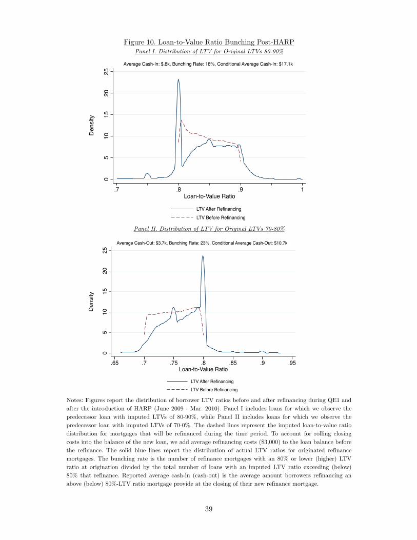
Figure 10. Loan-to-Value Ratio Bunching Post-HARPPanel I. Distribution of LTV for Original LTVs 80-90%

Panel II. Distribution of LTV for Original LTVs 70-80%

Notes: Figures report the distribution of borrower LTV ratios before and after refinancing during QE1 andafter the introduction of HARP (June 2009 - Mar. 2010). Panel I includes loans for which we observe thepredecessor loan with imputed LTVs of 80-90%, while Panel II includes loans for which we observe thepredecessor loan with imputed LTVs of 70-0%. The dashed lines represent the imputed loan-to-value ratiodistribution for mortgages that will be refinanced during the time period. To account for rolling closingcosts into the balance of the new loan, we add average refinancing costs ($3,000) to the loan balance beforethe refinance. The solid blue lines report the distribution of actual LTV ratios for originated refinancemortgages. The bunching rate is the number of refinance mortgages with an 80% or lower (higher) LTVratio at origination divided by the total number of loans with an imputed LTV ratio exceeding (below)80% that refinance. Reported average cash-in (cash-out) is the average amount borrowers refinancing anabove (below) 80%-LTV ratio mortgage provide at the closing of their new refinance mortgage.

05

1015

2025

Den

sity

.7 .8 .9 1Loan-to-Value Ratio

LTV After RefinancingLTV Before Refinancing

Average Cash-In: $.8k, Bunching Rate: 18%, Conditional Average Cash-In: $17.1k

05

1015

2025

Den

sity

.65 .7 .75 .8 .85 .9 .95Loan-to-Value Ratio

LTV After RefinancingLTV Before Refinancing

Average Cash-Out: $3.7k, Bunching Rate: 23%, Conditional Average Cash-Out: $10.7k

39

Notes: Figures plot distribution of loan sizes relative to the local conforming loan limit (CLL). The dashedline plots the distribution of normalized loan sizes for those borrowers with loan sizes above the CLL whorefinanced one quarter prior to refinancing. The solid line shows the distribution of normalized loan sizesfor the refinance mortgages of the borrowers whose predecessor loans are represented by the dashed line.The sample consists of refinance loans originated during 2008-2013 for which we observe the predecessorloan with outstanding principal between 100 and 140% of the local CLL (panel I) and loan whoseoutstanding balance (adjusted for expected refinancing costs) is between 80 and 100% of the CLL.

Figure 11. Conforming Loan Limit BunchingPanel I. Distribution of Loan Size/CLL for Original Balances 100-140% of CLL

Panel II. Distribution of Loan Size/CLL for Original Balances 80-100% of CLL

05

1015

2025

Den

sity

.8 .9 1 1.1 1.2 1.3 1.4 1.5Ratio of Loan Amount to Conforming Loan Limit

Loan Amount After Refinancing/CLLLoan Amount Before Refinancing/CLL

Average Cash-In: $27k, Bunching Rate: 43%, Conditional Average Cash-In: $81k

02

46

8

Den

sity

.6 .7 .8 .9 1 1.1Ratio of Loan Amount to Conforming Loan Limit

Loan Amount After Refinancing/CLLLoan Amount Before Refinancing/CLL

Average Cash-Out: $27k, Bunching Rate: 10%, Conditional Average Cash-Out: $21.5k

40

Count Mean Std. Dev. 1st 10th 50th 90th 99th

LTV 7,308,119 66.69 18.09 27.40 40.70 69.24 88.18 109.20FICO 7,308,076 751.90 51 594 681 766 804 819Interest Rate 6,374,466 4.56 0.96 2.75 3.38 4.50 5.75 7.13Balance 7,308,119 211,335 117,725 44,000 83,000 185,000 388,000 590,000

LTV 172,212 64.73 14.70 28.50 43.22 67.23 80.00 95.80FICO 150,730 761.30 36.02 660 709 770 800 814Interest Rate 172,182 4.10 1.14 1.88 2.75 3.88 5.63 7.25Balance 172,212 959,771 693,231 440,000 536,000 813,000 1,475,000 3,265,000

Guarantee fees 72 34.05 11.03 23.80 25.70 28.92 56.07 61.20Aaa Yields 72 4.74 0.74 3.40 3.73 4.95 5.57 6.28Baa Yields 72 6.08 1.13 4.51 4.85 5.97 8.06 9.21Baa-Aaa Spread 72 1.34 0.62 0.75 0.84 1.18 2.52 3.38Notes: Panel I & Panel II report loan-level summary statistics on conforming and jumbo loans from Equifax's CRISM database which merges McDashAnalytics mortgage servicing records from Lender Processing Services with Equifax credit bureau data. Panel III reports summary statistics for timeseries controls used in robustness checks, including guarantee fees from Fuster et al. (2013) and bond yields from Federal Reserve Economic Data(FRED) at the Federal Reserve Bank of St. Louis.

PercentileTable 1. Summary Statistics

Panel I. Below-Conforming Loan Limit Loans

Panel II. Jumbo Loans

Panel III. Spreads and Yields

(1) (2) (3) (4) (5) (6) (7) (8) (9) (10)Program

Program Indicator -107.514*** -35.232** -43.259*** -18.039** 25.265(13.549) (10.338) (7.020) (5.908) (13.656)

Program x Jumbo 48.562*** 41.809*** -3.812 -1.800 4.996*** 4.715 -0.013 -1.022 -21.153* -24.829**(6.441) (7.485) (5.927) (5.964) (1.141) (2.375) (1.506) (1.739) (8.415) (8.216)

Jumbo Indicator 29.946*** 33.178*** 46.548*** 47.363*** 20.755*** 23.204*** 25.964*** 28.176*** -1.706 0.63-5.466 -5.516 -3.739 -2.842 -1.152 -2.019 -1.131 -1.258 -3.359 -3.197

Controls Yes Yes Yes Yes Yes Yes Yes Yes Yes YesCounty x Month FEs Yes Yes Yes Yes YesObservations 331,895 331,895 292,290 292,290 180,055 180,055 201,060 201,060 262,493 262,493R-squared 0.564 0.669 0.297 0.457 0.364 0.462 0.219 0.336 0.203 0.383Notes: The table reports regression coefficients relating loan-level mortgage interest rates (in basis points) to the quantitative easing programs and to theother monetary policy programs. QE, MEP ("Maturity Extension Program"), and Tapering Indicators are dummy variables equal to one after theintroduction of each program (see Appendix Table 1). The sample includes single-family, first lien, 30-year term, fixed rate, non-interest only, non-balloon,and non-FHA refinance mortgages with no prepayment penalties and less than or equal to 80% LTV. Controls include binned original LTV and binnedcredit score. Jumbo Indicator is a dummy equal to one for jumbo loans. Program x Jumbo is the interaction between the program dummies and JumboIndicator. The sample includes single-family, first lien, non-FHA refinance mortgages. The event window includes the three months before/after thebeginning month of each program period (e.g. QE1 sample is Sep2008-Feb2009). All specifications control for 5-point LTV bins, 20-point FICO bins, and anindicator for missing FICO. Even columns control for county by month fixed effects. Standard errors are clustered at the month level. Asterisks denotesignificance levels (***=1%, **=5%, *=10%).

Table 2. Effect of QE Campaign Beginning on Interest Rates: 3-Month Window

QE1 QE2 MEP QE3 Tapering

(1) (2) (3) (4) (5) (6) (7) (8) (9) (10)Program

Program Indicator -128.508*** -45.511*** -60.346*** -32.475*** 50.168***(9.444) (8.374) (6.724) (5.830) (14.362)

Program x Jumbo 55.942*** 52.780*** -1.837 -1.324 10.885*** 10.058*** -3.331 -4.799 -33.257*** -35.631***(6.515) (5.841) (5.577) (5.309) (2.236) (2.407) (3.056) (2.944) (7.815) (6.683)

Jumbo Indicator 16.849** 20.154*** 44.125*** 52.756*** 17.125*** 19.849*** 25.421*** 27.578*** 7.092 8.752*(5.565) (4.724) (2.650) (8.614) (1.844) (2.100) (1.232) (0.801) (4.379) (4.244)

Controls Yes Yes Yes Yes Yes Yes Yes Yes Yes YesCounty*Month FEs Yes Yes Yes Yes YesObservations 789,945 789,945 568,776 568,776 351,042 351,042 438,201 438,201 470,820 470,820R-squared 0.669 0.745 0.362 0.493 0.478 0.576 0.304 0.428 0.360 0.567Notes: The table reports regression coefficients relating loan-level mortgage interest rates (in basis points) to the quantitative easing programs and to the othermonetary policy programs. QE, MEP ("Maturity Extension Program"), and Tapering Indicators are dummy variables equal to one after the introduction of eachprogram (see Appendix Table 1). The sample includes single-family, first lien, 30-year term, fixed rate, non-interest only, non-balloon, and non-FHA refinancemortgages with no prepayment penalties and less than or equal to 80% LTV. Controls include binned original LTV and binned credit score. Jumbo Indicator is adummy equal to one for jumbo loans. Program x Jumbo is the interaction between the program dummies and Jumbo Indicator. The sample includes single-family,first lien, non-FHA refinance mortgages. The event window includes the six months before/after the beginning month of each program period (e.g. QE1 sample isSep2008-Feb2009). All specifications control for LTV bins, FICO bins, and an indicator for missing FICO. Even columns control for county by month fixed effects.Standard errors are clustered at the month level. Asterisks denote significance levels (***=1%, **=5%, *=10%).

Table 3. Effect of QE Campaign Beginning on Interest Rates: 6-Month Window

QE1 QE2 MEP QE3 Tapering

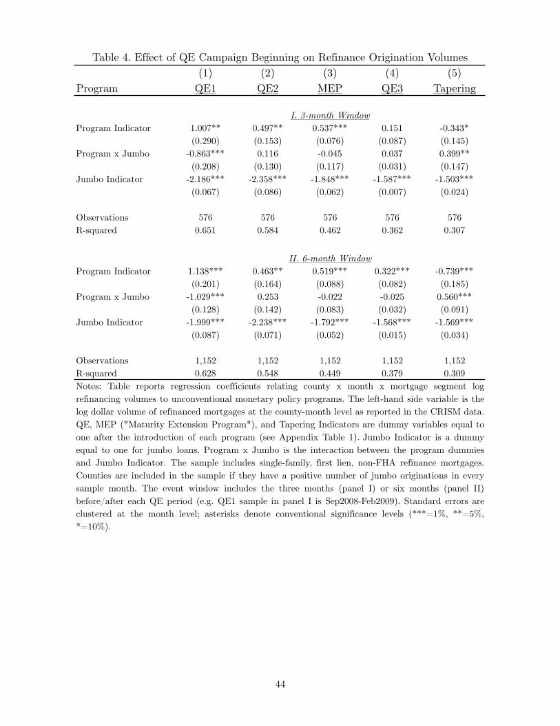
(1) (2) (3) (4) (5)Program QE1 QE2 MEP QE3 Tapering

Program Indicator 1.007** 0.497** 0.537*** 0.151 -0.343*(0.290) (0.153) (0.076) (0.087) (0.145)

Program x Jumbo -0.863*** 0.116 -0.045 0.037 0.399**(0.208) (0.130) (0.117) (0.031) (0.147)

Jumbo Indicator -2.186*** -2.358*** -1.848*** -1.587*** -1.503***(0.067) (0.086) (0.062) (0.007) (0.024)

Observations 576 576 576 576 576R-squared 0.651 0.584 0.462 0.362 0.307

Program Indicator 1.138*** 0.463** 0.519*** 0.322*** -0.739***(0.201) (0.164) (0.088) (0.082) (0.185)

Program x Jumbo -1.029*** 0.253 -0.022 -0.025 0.560***(0.128) (0.142) (0.083) (0.032) (0.091)

Jumbo Indicator -1.999*** -2.238*** -1.792*** -1.568*** -1.569***(0.087) (0.071) (0.052) (0.015) (0.034)

Observations 1,152 1,152 1,152 1,152 1,152R-squared 0.628 0.548 0.449 0.379 0.309

Table 4. Effect of QE Campaign Beginning on Refinance Origination Volumes

Notes: Table reports regression coefficients relating county x month x mortgage segment logrefinancing volumes to unconventional monetary policy programs. The left-hand side variable is thelog dollar volume of refinanced mortgages at the county-month level as reported in the CRISM data. QE, MEP ("Maturity Extension Program"), and Tapering Indicators are dummy variables equal toone after the introduction of each program (see Appendix Table 1). Jumbo Indicator is a dummyequal to one for jumbo loans. Program x Jumbo is the interaction between the program dummiesand Jumbo Indicator. The sample includes single-family, first lien, non-FHA refinance mortgages.Counties are included in the sample if they have a positive number of jumbo originations in everysample month. The event window includes the three months (panel I) or six months (panel II)before/after each QE period (e.g. QE1 sample in panel I is Sep2008-Feb2009). Standard errors areclustered at the month level; asterisks denote conventional significance levels (***=1%, **=5%,*=10%). 

I. 3-month Window

II. 6-month Window

44

(1) (2) (3) (4) (5)Program QE1 QE2 MEP QE3 Tapering

Program x Jumbo 29.259** -0.576 -4.564 5.878 -22.961**(7.555) (5.201) (3.295) (3.003) (7.414)

Jumbo Indicator -35.321*** 9.242 -4.417 10.396*** 10.823***(2.261) (4.596) (2.318) (0.918) (1.670)

Controls Yes Yes Yes Yes YesCounty*Month FEs Yes Yes Yes Yes YesObservations 331,895 292,290 180,055 201,060 262,493R-squared 0.668 0.450 0.462 0.326 0.381

Program x Jumbo -0.711* 0.056 0.160 -0.108 0.339(0.351) (0.185) (0.205) (0.091) (0.183)

Jumbo Indicator -2.419*** -2.432*** -2.363*** -2.044*** -3.178***(0.172) (0.140) (0.110) (0.022) (0.016)

County*Month FEs Yes Yes Yes Yes YesObservations 576 576 576 576 576R-squared 0.930 0.938 0.941 0.933 0.960

Table 5. Robustness to Controlling for G-Fees and Credit Spreads: 3-Month Window

Notes: Panel I reports regression coefficients relating interest rates to the quantitative easing programs and tothe other monetary policy programs. The sample includes single-family, first lien, 30-year term, fixed rate, non-interest only, non-balloon, and non-FHA refinance mortgages with no prepayment penalties and less than orequal to 80% LTV. Controls include binned original LTV and binned credit score. In all columns, we firstsubtract the contribution of the interaction of the Jumbo Indicator with a measure of Credit Spread (i.e. BBBto AAA spread from St. Louis Fed), with guarantee fees from Fuster et al. (2013), and county x month fixedeffects as described in section 6.1.3. Panel II reports regression coefficients relating refinancing volume to thequantitative easing programs and to the other monetary policy programs. The left hand side variable is definedas the log of the dollar volume of refinanced mortgages as reported in the CRISM data. The sample includessingle-family, first lien, non-FHA refinance mortgages. Counties are included in the quantity sample if they havegreater than one jumbo origination in every month. All columns control for county x month fixed effects. Weagain subtract the contribution of the interaction of the jumbo indicator with credit spread and with guaranteefees as described in section 6.1.3. QE, MEP ("Maturity Extension Program"), and Tapering Indicators aredummy variables equal to one after the introduction of each program. MEP begins in Sept. 2011. Taperingbegins in June 2013. Jumbo Indicator is a dummy equal to one for jumbo loans. QE x Jumbo is the interactionbetween the program dummies and Jumbo Indicator. The event window includes the three months prior to andafter the beginning month of each QE period. For example, QE1 begins in December 2008, and the eventwindow lasts from September 2008 through March 2009. Standard errors are clustered at the month level, andare reported in parentheses. Asterisks denote significance levels (***=1%, **=5%, *=10%). 

Panel I. Interest Rates

Panel II. Refinance Origination Volumes

45

(1) (2) (3)December 2008 Indicator 0.151*** 0.114** 0.108*

(0.033) (0.057) (0.063)January 2009 Indicator 0.812*** 0.954*** 0.950***

(0.027) (0.046) (0.051)February 2009 Indicator 1.245*** 1.367*** 1.372***

(0.025) (0.043) (0.047)Current LTV > .9 x December 2008 -0.064 -0.063

(0.086) (0.099)Current LTV > .9 x January 2009 -0.447*** -0.379***

(0.072) (0.081)Current LTV > .9 x February 2009 -0.429*** -0.376***

(0.065) (0.073)December 2008 x Jumbo 0.120 0.017

(0.086) (0.097)January 2009 x Jumbo -0.190** -0.212**

(0.076) (0.083)February 2009 x Jumbo -0.203*** -0.227***

(0.069) (0.075)

Loan Controls Yes Yes YesBorrower Controls YesObservations 1,691,380 1,691,380 1,407,066

Table 6. Hazard Model Estimates of QE1 Effect on Refinancing

Notes: Table reports maximum-likelihood estimates of the prepayment hazardmodel described in Section 5.3. All specifications include a cubic function of loanage as a non-parametric baseline hazard. Loan-level controls include currentLTV, loan size at origination, indicators for current LTV between 80 and 90%,current LTV over 90%, and current balance over the conforming loan limit.Borrower controls include DTI, a missing DTI indicator, and FICO bins. Jumbois an indicator for loan amount at least $60,000 above the CLL to account forcash-in refinancingRobust standard errors in parentheses.

46

Appendix

A Additional TBA Market Details

On the day a TBA contract is traded, the buyer and seller fix the basic characteristics of the MBS to

be delivered, with a 0.01% allowed variance in the par value at delivery. Sellers in the TBA market

are primarily mortgage originators seeking to lock in interest rates to hedge short-run interest-rate

risk. Buyers in this market include MBS sponsors who are assembling Collateralized Mortgage

Obligations for new securitizations. Generally, only six parameters of the mortgages to be delivered

are specified: agency (Fannie, Freddie, or Ginnie), weighted-average maturity, weighted-average

coupon (in 50 basis-point increments), price, par amount, and settlement date.23 A separate (much

smaller) market exists called the Stipulated (STIP) market where CMOs with detailed information

disclosures are traded. For this reason, when there is information to disclose about a MBS that

enhances its value (e.g., predictors of lower early-termination risk), the STIP market is a more

favorable trading platform.24 Two days prior to TBA settlement date, the seller informs the buyer

of the specific pools to be delivered and the trade is settled on an Agency-determined settlement

date. To deliver these pools, the seller has either acquired or originated Agency-eligible mortgages

and paid the necessary upfront fees (known as g-fees) to have them assembled into an Agency-

guaranteed pool. For a variety of reasons, the vast majority of mortgages comprising TBAs are

recent originations. Payment history information about seasoned mortgages can make them more

valuable to trade on the STIP market (in the case of good news) or ineligible for TBA inclusion

(in the case of missed payments, etc.). Adverse selection arising from the superior information set

of the seller as to the termination risk of the mortgages to be delivered is mitigated by “cheapest-

to-deliver” expectations and pricing by buyers and sellers (see Downing et al., 2009). This TBA

contract standardization effectively commoditizes the MBS traded in TBAs, providing the TBA

market with a degree of liquidity unmatched by any other secondary mortgage market, meaning

23For example, a TBA contract might be simply specified FN3060, meaning that it represents a Fannie Mae-guaranteed MBS whose weighted average maturity and coupon are 30 years and 4.0%, respectively. Although rare,some additional characteristics may be specified, for example, the number of pools in a security, geographic compo-sition, etc.

24In the Agency market, due to the default guarantees provided by Fannie, Freddie, and Ginnie, the value ofMBS will primarily vary with the degree of termination risk borne by the investor since to the holder of a Agency-guaranteed mortgage, the cash flows from default and prepayment look identical. This risk may be a function ofother features of the MBS not stipulated on the TBA forward contract, such as FICO, DTI, geographic location, etc.

47

that even legal requirements aside, purchasing TBAs was the only feasible option at the time.25

B Robustness to Increasing Conforming Loan Limits

In this appendix, we investigate the concern that the stronger response of GSE-eligible originations

relative to jumbo originations around QE event dates simply reflects the establishment of high-cost

area designations. The conforming loan limit increased from about $400,000 to $700,000 for certain

high-cost areas over time (see Panel I of Appendix Figure 1). As mapped in Panel II of Appendix

Figure 1, these areas are mainly counties on the coasts that have higher land values. Although this

increase occurred nearly a year before the beginning of QE1, expanding the size of the conforming

market by increasing the CLL in certain areas should tilt originations from the jumbo segment

to the GSE-eligible segment. To address this concern, we restrict our attention to the counties

that remained exclusively in the low-cost areas that have had no increase in their CLLs since 2006.

Appendix Figure 2 shows that even when we restrict attention to these areas, we observe a significant

and differential increase in the origination of conforming loans around QE1. We find that for the

period before the expiration the jumbo and conforming segments track each other closely, except

for the QE1 period.

25While each mortgage is a highly differentiated product, all mortgages in a given TBA contract are essentiallybehind a veil of ignorance and can thus be traded as a commodity. For market participants, the risk managementand valuation exercises are simplified as they need consider only the risks associated with the main characteristics ofthe MBS. See Vickery and Wright (2013), who quantify the magnitude of the liquidity benefits of the TBA market,and Glaeser and Kallal (1997) and Vanasco (2014) for theoretical treatments of this benefit. However, this fungibilityis temporary. Upon settlement and delivery, the buyer observes the complete set of characteristics of each loan pooland the market value of delivered mortgage-backed securities will incorporate this information.

48

Appendix Figure 1. Conforming Loan Limits

Notes: Panel I plots the national conforming loan limit over time and its maximal increase among certainhigh-cost counties in early 2008. Some of these temporary high-cost exemptions expired on October 1,2011. Panel II plots all counties in the contiguous state. Darkly shaded areas indicate counties designatedas high cost, defined as counties with conforming loan limits greater than $417,000.

Panel II. The Geography of High-Cost County Designation

Panel I. National and Maximum High-Cost Area Conforming Loan Limits

$0

$100,000

$200,000

$300,000

$400,000

$500,000

$600,000

$700,000

$800,000

National CLL County-Varying Max CLL

49

Notes: Figure plots the count of refinance mortgage originations in low-cost areas recorded by LPS forloans below and above the GSE conforming loan limit (CLL). See notes for Figure 6.

Appendix Figure 2. Refinance Origination Count in Low-Cost Areas

50

Episode Announcement Date Event Event Date

QE1.1 25-Nov-08 QE 1 Start Dec-2008QE1.2 1-Dec-08QE1.3 16-Dec-08QE1.4 28-Jan-09QE1.5 18-Mar-09QE1.6 23-Sep-09 QE 1 End Apr-2010QE2.1 10-Aug-10 QE 2 Start Sep-2010QE2.2 21-Sep-10 QE 2 End Jul-2011FG.1 9-Aug-11 MEP Start Sep-2011FG.2 25-Jan-12QE3.1 13-Sep-12 QE 3 Start Sep-2012QE3.2 22-May-13QE3.3 19-Jun-13 Tapering Jun-2013QE3.4 10-Jul-13QE3.5 18-Sep-13 QE 3 End Oct-2014

Note: Table reports the timing of Federal Reserve Quantitative Easing announcements fromKrishnamurthy and Vissing-Jorgensen (2011) and Krishnamurthy and Vissing-Jorgensen (2013) aswell as the dates used in the paper for each LSAP program.

Appendix Table 1. Fed Unconventional Monetary Policy Announcement Dates and Dates Used in Analysis

51

30-Yr FRM <30-Yr FRM ARM FHA IO Other Total

30-Year FRM 33.47% 14.08% 2.32% 3.25% 1.03% 0.21% 54.36%<30-Year FRM 4.60% 12.20% 0.49% 0.76% 0.26% 0.04% 18.35%ARM 5.27% 0.92% 2.03% 0.72% 1.75% 0.19% 10.89%FHA 1.40% 0.76% 0.16% 7.58% 0.07% 0.03% 9.99%IO 2.90% 0.27% 0.64% 0.38% 1.66% 0.07% 5.93%Other 0.25% 0.09% 0.03% 0.07% 0.02% 0.02% 0.49%Total 47.89% 28.33% 5.67% 12.77% 4.79% 0.55% 100.00%

30-Year FRM 20.20% 3.66% 4.45% 0.63% 4.14% 0.66% 33.75%<30-Year FRM 6.52% 5.95% 1.03% 0.16% 1.05% 0.10% 14.80%ARM 13.45% 1.59% 8.14% 0.49% 8.06% 0.88% 32.61%FHA 3.04% 0.83% 1.01% 1.76% 0.46% 0.12% 7.23%IO 3.32% 0.30% 2.46% 0.07% 4.63% 0.27% 11.04%Other 0.22% 0.22% 0.07% 0.01% 0.04% 0.02% 0.58%Total 46.75% 12.56% 17.15% 3.12% 18.37% 2.05% 100.00%

30-Year FRM 24.62% 3.82% 1.29% 1.38% 3.73% 0.90% 35.73%<30-Year FRM 7.21% 6.24% 0.27% 0.29% 0.85% 0.11% 14.98%ARM 16.71% 1.94% 3.02% 1.49% 7.22% 0.91% 31.28%FHA 2.49% 0.73% 0.18% 1.89% 0.22% 0.11% 5.62%IO 4.73% 0.30% 0.88% 0.30% 4.88% 0.34% 11.43%Other 0.47% 0.15% 0.06% 0.06% 0.12% 0.10% 0.95%Total 56.22% 13.18% 5.70% 5.41% 17.02% 2.47% 100.00%

30-Year FRM 28.70% 7.91% 0.78% 7.46% 1.01% 0.20% 46.06%<30-Year FRM 6.13% 9.29% 0.22% 1.57% 0.25% 0.04% 17.49%ARM 9.48% 1.87% 1.24% 3.21% 1.59% 0.08% 17.45%FHA 1.21% 0.75% 0.05% 5.68% 0.02% 0.02% 7.73%IO 5.03% 0.44% 0.42% 1.24% 2.72% 0.05% 9.91%Other 0.69% 0.19% 0.03% 0.35% 0.06% 0.03% 1.35%Total 51.24% 20.45% 2.74% 19.50% 5.65% 0.42% 100.00%

30-Year FRM 39.53% 9.26% 0.95% 6.44% 0.16% 0.05% 56.38%<30-Year FRM 5.60% 8.91% 0.17% 1.38% 0.05% 0.02% 16.14%ARM 3.59% 0.67% 0.48% 0.71% 0.13% 0.02% 5.61%FHA 0.62% 0.38% 0.01% 15.09% 0.00% 0.00% 16.10%IO 3.63% 0.26% 0.23% 0.68% 0.62% 0.01% 5.43%Other 0.19% 0.04% 0.00% 0.11% 0.00% 0.00% 0.35%Total 53.17% 19.51% 1.85% 24.41% 0.96% 0.11% 100.00%

(continued on next page)

Panel III. 2007

Orig

inal

Mor

tgag

e

Panel IV. 2008

Orig

inal

Mor

tgag

e

Panel V. 2009

Orig

inal

Mor

tgag

e

Appendix Table 2. Mortgage Product Refinancing Transition MatrixRefinance Mortgage

Panel I. Total 2006–2013

Orig

inal

Mor

tgag

e

Panel II. 2006

Orig

inal

Mor

tgag

e

52

30-Yr FRM <30-Yr FRM ARM FHA IO Other Total

30-Year FRM 35.07% 17.71% 3.06% 4.48% 0.21% 0.07% 60.60%<30-Year FRM 3.73% 14.53% 0.59% 1.10% 0.06% 0.03% 20.04%ARM 1.69% 0.58% 1.16% 0.30% 0.10% 0.02% 3.84%FHA 0.69% 0.57% 0.04% 9.28% 0.00% 0.00% 10.58%IO 2.63% 0.29% 0.55% 0.44% 0.74% 0.01% 4.68%Other 0.16% 0.04% 0.01% 0.05% 0.00% 0.00% 0.27%Total 43.98% 33.72% 5.40% 15.65% 1.12% 0.14% 100.00%

30-Year FRM 33.29% 20.38% 4.88% 2.72% 0.29% 0.10% 61.66%<30-Year FRM 3.46% 17.97% 0.98% 0.79% 0.10% 0.04% 23.33%ARM 1.13% 0.49% 1.69% 0.17% 0.11% 0.02% 3.61%FHA 0.90% 0.89% 0.10% 5.42% 0.00% 0.01% 7.32%IO 1.86% 0.26% 0.76% 0.19% 0.77% 0.02% 3.85%Other 0.13% 0.05% 0.01% 0.02% 0.00% 0.00% 0.23%Total 40.78% 40.04% 8.43% 9.30% 1.27% 0.18% 100.00%

30-Year FRM 40.77% 21.81% 2.76% 0.83% 0.24% 0.02% 66.43%<30-Year FRM 2.55% 16.49% 0.59% 0.30% 0.08% 0.00% 20.02%ARM 0.93% 0.38% 1.26% 0.04% 0.08% 0.00% 2.69%FHA 1.11% 0.85% 0.06% 6.28% 0.00% 0.00% 8.31%IO 1.29% 0.18% 0.27% 0.03% 0.53% 0.00% 2.30%Other 0.15% 0.06% 0.03% 0.01% 0.00% 0.00% 0.25%Total 46.81% 39.77% 4.98% 7.49% 0.93% 0.03% 100.00%

30-Year FRM 36.26% 24.16% 1.47% 0.56% 0.17% 0.00% 62.62%<30-Year FRM 2.57% 16.76% 0.31% 0.19% 0.06% 0.00% 19.88%ARM 1.24% 0.54% 1.48% 0.05% 0.10% 0.00% 3.42%FHA 1.97% 1.24% 0.10% 8.14% 0.01% 0.00% 11.46%IO 1.32% 0.20% 0.26% 0.03% 0.53% 0.00% 2.34%Other 0.18% 0.07% 0.03% 0.01% 0.00% 0.00% 0.29%Total 43.53% 42.98% 3.65% 8.97% 0.86% 0.00% 100.00%

Panel VII. 2011

Orig

inal

Mor

tgag

e

Panel VI. 2010

Orig

inal

Mor

tgag

e

Appendix Table 2 (cont.). Mortgage Product Refinancing Transition MatrixRefinance Mortgage

Panel VIII. 2012

Orig

inal

Mor

tgag

e

Panel IV. 2013

Orig

inal

Mor

tgag

e

Notes: Table reports the percent of first-lien mortgages refinancing from a given original mortgage type (row) in a given year (panel) into the given refinance mortgage product type (column) from 2006 and 2013. Mortgage product categories are mutually exclusive. 30-Year FRM includes all non-FHA fixed-rate mortgages with original term of exactly 30 years. <30-Year FRM includes non-FHA fixed-rate mortgages with original terms under 30 years. ARM includes non-interest-only and non-FHA adjustable-rate mortgages. FHA includes all Federal Housing Administration loans, regarless of other product characteristics. IO includes all non-FHA interest only loans. Other includes various other product types including, for example, fixed-rate loans with an original term over 30 years. Source: LPS and Equifax.

53

(1) (2) (3) (4) (5)Program QE1 QE2 MEP QE3 Tapering

Program x Jumbo 26.039*** -1.594 2.015 12.839*** -25.011***(4.124) (4.654) (3.865) (3.015) (5.065)

Jumbo Indicator -32.950*** 6.599* -10.550** 5.174* 12.100***(2.718) (3.220) (3.661) (2.616) (1.138)

Controls Yes Yes Yes Yes YesCounty x Month FEs Yes Yes Yes Yes YesObservations 789,945 568,776 351,042 438,201 470,820R-squared 0.744 0.489 0.577 0.419 0.569

Program x Jumbo -0.788*** 0.239 0.166 -0.337** 0.239(0.180) (0.184) (0.158) (0.126) (0.148)

Jumbo Indicator -2.318*** -2.374*** -2.258*** -1.957*** -3.053***(0.103) (0.088) (0.110) (0.060) (0.105)

Controls Yes Yes Yes Yes YesCounty x Month FEs Yes Yes Yes Yes YesObservations 1,152 1,152 1,152 1,152 1,152R-squared 0.939 0.934 0.938 0.933 0.958

Appendix Table 3. Robustness to G-Fees and Credit Spreads: 6-Month Window

Notes: Panel I reports regression coefficients relating interest rates to the quantitative easing programsand to the other monetary policy programs. The sample includes single-family, first lien, 30-year term,fixed rate, non-interest only, non-balloon, and non-FHA refinance mortgages with no prepaymentpenalties with less than or equal to 80% LTV. Controls include binned original LTV and credit score. Inall columns, we subtract the contribution of an interaction of the Jumbo Indicator with a measure ofCredit Spread (i.e. BBB to AAA spread) and with guarantee fees as described in section 6.1.3 as well ascounty by month fixed effects. Panel II reports regression coefficients relating refinancing volume to thequantitative easing programs and to the other monetary policy programs. The left hand side variable isdefined as the log of the dollar volume of refinanced mortgages as reported in the CRISM data. Thesample includes single-family, first lien, non-FHA refinance mortgages. Counties are included in thesample that have positive jumbo originations every month. In all odd columns, we control for theinteraction between county fixed effects and the Jumbo Indicator, while in all even columns, we controlfor county by month fixed effects. In both Panel I & II for all columns, we control for the interaction ofthe jumbo indicator with a measure of Credit Spread (i.e. BBB to AAA spread) and with guaranteefees. QE, MEP ("Maturity Extension Program"), and Tapering Indicators are dummy variables equal toone after the introduction of each program. MEP begins in Sept. 2011. Tapering begins in July2013. Jumbo Indicator is a dummy equal to one for jumbo loans. QE x Jumbo is the interactionbetween the program dummies and Jumbo Indicator. The event window includes the six months prior toand after the beginning month of each QE period. For example, QE1 begins in December 2008, and theevent window lasts from June 2008 through June 2009. Standard errors are clustered at the month level,and are reported in parentheses. Asterisks denote significance levels (***=1%, **=5%, *=10%). 

Panel I. Interest Rates

Panel II. Refinance Origination Volumes

54

(1) (2) (3) (4) (5)QE1 QE2 MEP QE3 Tapering

25.19*** 20.45*** 17.71*** 19.51*** 20.40***(6.01) (2.84) (2.68) (2.62) (2.68)

-1.48*** -1.43*** -1.61*** -1.61*** -1.32***(0.16) (0.19) (0.17) (0.17) (0.31)

48.33*** 50.33*** 62.71*** 55.87*** 47.32***(9.88) (8.73) (7.64) (6.92) (9.40)

County-Month FEs Yes Yes Yes Yes YesObservations 2,618,508 2,839,677 3,057,411 2,970,252 2,937,633R-squared 0.781 0.799 0.788 0.740 0.748

-0.25 -0.45*** -0.42*** -0.44*** -0.45***(0.18) (0.08) (0.09) (0.08) (0.08)

0.03*** 0.02*** 0.03*** 0.03*** 0.04***(0.00) (0.00) (0.00) (0.00) (0.00)

County-Month FEs Yes Yes Yes Yes YesObservations 5,760 5,760 5,760 5,760 5,760R-squared 0.937 0.929 0.931 0.930 0.93

AB Spread × Jumbo

G-Fee × Jumbo

Notes: Each column estimates the relationship between interest rates (panel I) and originationvolumes (panel II) to credit spreads and guarantee fees for all months between 2008-2013 except forthe six months before/after the indicated program. The sample for panel I includes loans with LTVless than or equal to 80%, controlling for county by month fixed effects. The sample for panel II hastwo observations for each county-month: log of total refinance origination below the conforming loanlimit and above the conforming loan limit for counties that had non-zero refinancing activity in boththe jumbo and non-jumbo segments throughout the sample period. We control for county by monthfixed effects. QE1 begins in December 2008, QE2 begins in September 2010, MEP begins inSeptember 2011, QE3 begins in September 2012, and Tapering begins in June 2013. Clusteredstandard errors are reported in parentheses. Asterisks denote significance levels (***=1%, **=5%,*=10%).

Appendix Table 4. Coefficients on AAA-BBB Spread and Guarantee Fee

AB Spread × Jumbo

G-Fee × Jumbo

Jumbo Indicator

Panel I. Interest Rates

Panel II. Refinance Origination Volume

55