Unconventional Gas Production:

Hydrated Gas

By:

James Mansingh

Jeffrey Melland

1

Summary........................................................................................................ 2 Introduction................................................................................................... 3 Background ................................................................................................... 3

Figure 1: Hydrate Stability Curve............................................................... 4 Results ............................................................................................................ 6

Locating ......................................................................................................................... 6 Drilling ........................................................................................................................... 7

Drilling and Measurements..................................................................................... 8 Reservoir Evaluation and Wireline......................................................................... 8 Well Service............................................................................................................ 9

Production ................................................................................................................... 10 Figure 2: Production rate vs. time............................................................ 16 Figure 3: Volume produced over time ..................................................... 17 Figure 4: Production rates......................................................................... 18

Pipeline......................................................................................................................... 18 TEG Dehydration Station ..................................................................................... 19

Figure 5: Dehydration unit....................................................................... 19 Large Compressor Station..................................................................................... 20

Figure 6: Large compressor station.......................................................... 20 Figure 7: Pipeline...................................................................................... 22 Figure 8: Small compressor station........................................................... 23 Figure 9: Pipeline flowchart...................................................................... 24

LNG Plant.................................................................................................................... 24 Figure 10: LNG plant................................................................................ 25

Delivery ........................................................................................................................ 26 Table 1: Delivery ...................................................................................... 27

Regasification Plant .................................................................................................... 28 Figure 11: Regasification PFD.................................................................. 28

Pipeline to China................................................................................................... 28 Procedure Summary.............................................................................................. 30

Figure 12: Storage Tanks .......................................................................... 31 Recommendations....................................................................................... 31 Works Cited................................................................................................. 33

2

Summary

The recovery of hydrated gas is not only a feasible source of energy, but has great potential for becoming a major source of income in the gas industry. The analysis of this report has determined that the exploration of Russian hydrate reserves, on the Kamchatkan peninsula specifically, and delivery to the Japanese market show earnings potential in the multi-billion dollar range. The greatest part of the production cost is going to be liquefying the gas for overseas transport. The next largest cost is piping the gas from the well-head to the liquefaction facility. It is recommended to build the liquefaction and regasification plants to handle rates to keep three LNG transport ships moving, or approximately 450,000 kg/hour methane. The risk curve and regret analysis agree in this respect. Production costs at the LNG and regasification plant will run approximately $2.00 and $0.13 per MM Btu respectively. To keep the necessary rates, 22 wells over a 15 year period will be drilled in Kamchatka; this comes to $0.06 per MM Btu. The costs associated with piping gas from the well-head to the plant and then shipping to Japan are also relatively minor, only $0.64 and $0.53 per MM Btu respectively. Bringing the total production cost to $3.36 per MM Btu. Expected gas production rates average 135 million MM Btu per year, and at an average price of $7 per MM Btu, all investment money will be returned by year five. A yearly ROI of 14% is expected, with a final cash position of $6 billion at the end of 15 years. Assuming an inflation rate of 4%, the net present worth of this project is $3.5 billion dollars after this time period.

3

Introduction

Methane hydrates are found primarily in the arctic and Antarctic regions; in

permafrost and at the bottom of the ocean. A hydrate, or clathrate, is a cubic water

crystal with methane, ethane, or even larger hydrocarbon particles trapped inside of

the crystal structure. It is estimated that 165 standard volumetric units of gas are

trapped in one volumetric unit of hydrate. The permafrost hydrates are typically

found in porous sandstone. They are known to cap of free gas reservoirs; this would

be the source of the natural gas trapped in hydrate form. Hydrated gas reserves are

currently approximated between 100,000 and 270,000,000 trillion standard cubic feet

(TCF).

Hydrate reserves hold very real potential as a long term source of natural gas, but

is the current economic and technological environment suitable for hydrated gas

production and delivery? Two facts make hydrated gas typically unconventional for

production; it exists in solid form in the ground and deepwater, and it is found in

unpopulated regions of the planet. Despite these two facts, can hydrated gas

production be profitable now?

Background

Hydrates have posed a problem to the oil industry for years. Forty years ago the

main concern with hydrated gas is the problems it causes when it forms in oil and gas

lines. This would happen if there was significant solid hydrate coming out of the

well; after going through an expansion, the cooling effects would cause hydrate

formation growth within the pipe of casing. Now hydrated gas is being studied as a

4

possible source of natural gas or even as a way to transport natural gas as a solid. The

formation of hydrates is a more complex process than the dissociation thereof. The

formation reaction requires long periods of time in super gas saturated water to form

the first hydrate crystals, but once the seed crystals are present, hydrate growth may

speed up rapidly depending on conditions. The dissociation is much simpler and is

primarily a function of pressure. An Empirical formula (Chacin 31) found from

experimental data was found to be

87.331

3.7657)ln( +−=T

P ondissociati (1)

Where:

P = pressure (psi)

T = temperature (K)

The equilibrium curve looks like

0.00

5000.00

10000.00

15000.00

20000.00

25000.00

30000.00

35000.00

240 250 260 270 280 290 300 310

T (K)

P (kP

a)

Figure 1: Hydrate Stability Curve

Stable hydrated gas zone

Unstable hydrated gas zone

5

Clathrates are unstable at standard temperature and pressure and will dissociate fast

enough to support its own combustion. This is part of the basis for assumptions made

about the kinetics of the reaction later in this report.

The first problem facing the production of hydrated gas is that it exists as a solid.

Focusing on clathrates found on land, there are two methods to harvest the hydrate.

The first is to dig a hole and remove the solid hydrate, similar to coal mining. Since

hydrates are unstable at standard pressure and temperature, there are problems

associated with mining it as a mineral. These include miner suffocation, all of the fire

dangers associated with flammable gasses, not to mention all of the natural gas that

will escape the mine uncontrolled into the atmosphere. Mining is not only a

dangerous recovery method, it is also wasteful.

The second method is to drill a small hole, equalize the pressure on the formation

with atmospheric pressure, and allow the freed gas to flow from the high pressure

well to the low pressure pipeline. The second method of recovery is exclusively

studied in this report. The other problem with hydrated gas production is the remote

location of clathrate reserves. Since these reserves are not in close proximity to any

major markets, transportation costs are going to factor heavily into economical

calculations. The way to minimize these is to transport more of the product in one

trip; in other words more sales per trip. Recent developments in technology have

improved the cost effectiveness of the liquefaction of natural gas. Liquefied natural

gas (LNG) has a density many times that of compressed natural (CNG) and is stored

at low pressures, about one atmosphere. By liquefying natural gas, it becomes much

more easily shipped overseas in massive tankers. The region of interest in this report

6

is Kamchatka, Russia, a peninsula on the east coast of Russia north of Korea and

Japan. This is a convenient location for the exploration of hydrated gas for two

reasons; proximity to the ocean and Japan, which happens to be one of the hottest

markets for LNG. A relatively short pipeline is all that will be needed to transport

CNG from a well to the liquefaction plant on the coast. After the gas has been

liquefied, it can be loaded up onto a large LNG tanker and shipped to Japan. It takes

a gas flow rate of 3.5 MM scm per day to keep one LNG ship running at full capacity,

so multiples of this flow rate are used in the cost analysis and economic optimization.

For this project, three LNG ships running at full capacity give the best ROI and NPW.

Now that the flow rates to be analyzed, method of recovery, the transportation mode,

the hydrate location, and the market have been identified; an in depth cost analysis

can preformed to determine the economic potential of hydrated gas production in

Kamchatka, Russia.

Results

Locating

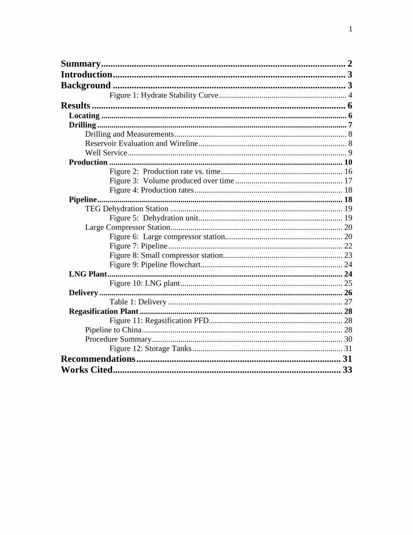
Large reserves of hydrated gas are believed to be located in Kamchatka. Hydrate

formations have been found, but extensive mapping and assessment of the reserves

have not been preformed. Large reserves have been surveyed in North Slope, Alaska

and the Mackenzie Delta, Canada. The Cherskiy mountain range in Kamchatka is the

location where seismic surveying will be performed. The hydrates can be found in

permafrost formations, but no detailed geological surveys of the area are reflected in

this report. Geophysical logs and seismic surveys are used to locate possible hydrate

7

bearing formations. Surveying a 400m to 1000m depth with an area of 2000 square

km will cost around $13 million. This is based on the cost to shoot a “block”; which

measures as three square miles and costs $30,000. The labor for the proposed depth,

area survey and processing costs will cost roughly $15 million (Pereira). The survey

should take about 6-8 weeks with a three man geological team.

Drilling

Drilling the well was broken up into three different segments. The total drilling

cost consisted of a sum of each segment. Rough cost estimates from a Schlumberger

catalog were used for each of the three different drilling segments: drilling, logging,

stimulation. The drilling cost per MM Btu is the cheapest step with a total capital

investment of $20.5 million and an operating cost of $0.06 per MMBtu. Each well

8

will cost $6.8 million to produce. Twenty-two wells will be drilled and produced

throughout the 15 year project.

Drilling and Measurements

Tools for drilling include drill bits, drill piping, rotary tables, drilling rigs, drilling

mud, and monitoring equipment. The drill bit is turned by drill piping which is

turned by the rotary table. Drill piping is attached in standard length segments to

increase the depth of the well drilled. Drilling mud is circulated through the drill

pipe and annulus of the hole to remove the rock cuttings from the hole well as create

a layer of mud cake against the formation. Many well site services are outsourced

and must be coordinated together in a consistent time frame or risk losing expensive

time for drilling. For example poorly designed mud can result in a drill pipe pin or

sabotage the quality of well logs upon completion. Costs are based on a combination

of equipment needed, mileage to job site, and days spent on site. The days spent on

site are based on a rate of penetration (ROP) of 90fph until reaching the hydrate

formation. This encompasses the first 1200ft, and then an ROP through the hydrate

formation is estimated to be 10fph. This drilling rate will continue until reaching

3300ft. This can become costly due to the possibility of increases in drilling time and

miscellaneous well site charges. A total of 343hrs plus 48 hrs to rig up and down is

based on an experienced crew for 17 days total drilling on one well. Total unit cost

for drilling and measurements comes to $895,000.

Reservoir Evaluation and Wireline

9

The logging truck is the operational center for wireline and evaluation, from

where the winch is controlled and operational control of the toolstring is performed.

The toolstring is a mechanical elongated cylinder powered by electrical current and

radiation sources. The toolstring collects data of resistivity, gamma ray, porosity and

sends them up via electrical signals in the cable to the logging truck. Wireline costs

are based on the factors similar to drilling and measurements. Log costs are based

upon the resolution of the logs taken. The slower the rate at which the tool string is

moved through the reservoir the better the resolution of the reservoir data. The basic

method of operation is to log a quick rough evaluation while going down hole. When

reaching the bottom the depth is calculated and the high resolution logging begins.

The two logs are compared to make sure the tool string equipment is working

properly. A charge of $5.95 per foot for the Highly Integrated Logging Tool (HILT)

or $6.43 per foot for the Formation Magnetic Imager (FMI) includes both up and

down logs as well as about a 100ft down hole repass log to ensure the tool string is

working properly. Total time on the job is not cost related unless the wireline team is

waiting on the rig crew, in which case an hourly standby cost of $1000 is applied.

The time frame to complete this logging can vary due to unforeseen circumstances

but two days for both cased hole and open hole operations is a reasonable assumption.

Total unit cost for wireline and logging is $15,000.

Well Service

Well Service will perform two jobs; first cementing the well for zone isolation,

and then fracturing the well to stimulate production. Cementing a well is a quick

operation. Equipment includes cement trucks and pump trucks. The manpower for

10

this operation is much smaller consisting of 1 operator and about 4-5 trucks.

Cementing ensures that there is no communication of gas between low and high

pressure zones, and is required for any well; as shallow the hydrates are, one day of

cementing will suffice. Two days to fracture the well is also a reasonable solution.

Fracturing the well is the most expensive, but arguably the most important part of

drilling. By fracturing the formation out from the well, the surface area through

which gas can flow is increased a hundred times. Costs for fracturing include

chemicals, personnel, and horsepower. The total unit cost for cementing and

stimulation services is $5,840,000.

Well Completion

The well is producing by this point so the job is to ensure good flow is achieved

and monitor well performance. Equipment consists of monitoring equipment,

temporary holding tanks and a compressor. Well completion cost is $68,000,

bringing the total cost of drilling one well to $6.8 million. Production rates will be

maintained initially around 10.5 million cubic meters per day, 22 wells are to be

drilled, and each will continue producing for the duration of the 15 year project.

Production

A existing model for the dissociation of hydrated gas locked in a rock formation

could not be found. The first thing to do is to make some simplifying assumptions.

The two most important assumptions are that 1 m3 of hydrate will release 165 scm of

gas, and the formation behaves as a closed tank with an expanding boundary. Other

minor assumptions include a homogenous and isotropic formation, no intermediate

phases, and rock expansion is negligible. The velocity of the moving hydrate

11

boundary is slow enough that the heat flux from the surrounding formation is

assumed to be enough to keep the process isothermal. The fracture is modeled by 2

wings 300 m long, 180° apart along the fracture gradient, running the entire depth of

the formation.

It is safe to assume a negligible pressure gradient along fractures. In a hydrate

formation there is typically a free gas zone trapped beneath a layer of hydrates, which

was the original source of the methane trapped in the hydrate formation. For the sake

of simplicity, this deals with the hydrate zone exclusively and ignores the effects of

the free gas zone.

Hydrated gas

X

Gas flow

Gfg

Gp

Qg

12

The second thing that should be studied is the kinetics of clathrate dissociation.

The equation for the movement of the hydrate boundary was found in Sloan (156)

( )∞

−

−= ffeKdt

dXeH

RT

E

s0 (2)

Where:

K0 = 1.5639107, m/(MPa s)

X = spatial position of the hydrate boundary, m

E = 17,776 kJ/kmol (CH4)

Ts = equilibrium temperature at system pressure, K

feH = equilibrium fugacity of methane at interface, MPa

f∞ = fugacity of methane in bulk gas phase, MPa

The kinetics of the dissociation proceed at a rate faster than that of the gas flow

through the formation, so for this model the hydrate is assumed to dissociate fast

enough to be in equilibrium at any point in time.

Assuming methane is the only significant component in the gas phase, the

fugacity terms become the dissociation pressure and the bulk gas pressure.

According to the kinetics the hydrate dissociation is very rapid. So the production

limiting resistance is assumed to be the flow through the formation, and pressure is

assumed to be the driving force. Using a Fourier type flux relationship

PkA

Qg ∇= (3)

Where:

Qg = flow rate out of the well, scm/s

k = well’s deliverability constant, scm/(MPa s m2)

13

It will be assumed that the pressure decreases linearly with distance where the ∆P the

difference between the well flowing pressure, Pwf, and the hydrate dissociation

pressure, PeH.

( )( ) wfeH

wf

PCXPXP

PCxxP

xCP

Cdx

dPP

+==

+=∆=∆

==∇

X

PPC wfeH −

= (4)

Assuming that the hydrate boundary moves in a direction perpendicular to the

fracture, X is the position of the hydrate surface measured from the fracture, while x

is a point in between the hydrate surface and the fracture. So now the pressure

gradient becomes a function of the position of the hydrate surface.

( ) ( )wf

wfeH PX

PPxxP +

−=

( )

X

PPP wfeH −

=∇

PkA

QgH ∇=

The area of flux is also dependent on X, so using this relatively simple model, we can

find the rate of production for varying formation deliverability constants at any

position X. Choosing the distance, X, we can find the pressure gradient, and the

respective production rate. Next we find a relationship for the GeH and Gp.

( ) fPeH GGG =− (5)

14

Where Gf is the moles of free gas trapped in the formation between the hydrate

boundary, and the well casing. Using the ideal gas law, we can integrate the pressure

gradient to find amount of free gas trapped in the formation.

( )

( )

+ℜ

=

+

−ℜ

=

+

−ℜ

=

ℜ=

∫

∫

2

2

2

0

wfeHff

wfwfeH

f

X

wfwfeH

f

f

PP

T

VG

XPX

PPX

T

AG

dxPX

PPx

T

AG

PdxT

AG

+ℜ

=2

wfeHff

PP

T

VG (6)

This takes into account gas trapped in all of the freed volume, Vf, in the formation.

The free volume is taken as a rectangular box with a height equal to the hydrate

formation height, one side equal to 2R, 600 m, and the last side equal to the distance

2X, that the hydrate boundary has moved. This rectangular box is capped at each

fracture end by half of a cylinder with a height equal to that of the formation and a

radius of X.

The equation for Vf is now

Vf = Hhydrate(4RX +R2π) (7)

An implicit assumption is that the water released form the dissociation falls into the

free gas zone and does not influence the production rates. The number of moles of

gas released from hydrate dissociation is easier to find using the first assumption.

15

STP

STPfeH T

PVG

ℜ=

165 (8)

This is the equation for number of moles methane released from formation. Now we

know the number of moles of gas produced as a function of X.

+ℜ

−ℜ

=2

165 wfeHf

STP

STPfP

PP

T

V

T

PVG (9)

Now know in Gp and Qg as a function of X we can numerically integrate using a

finite difference method to find the time involved in production. First specify X, find

Gp, and then using different k values find the time required for the change in Gp at a

constant Qg.

dt

dGQ P

g = (10)

Actual production rates with varying well deliverability over time look like

16

1.00E+05

1.00E+06

1.00E+07

0.1 1 10 100

t (months)

Qg

(sc

m/d

ay)

k = 0.003 scm/(s m2 Mpa) k = 0.004 scm/(s m2 Mpa) k = 0.005 scm/(s m2 Mpa)

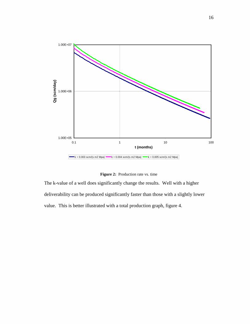
Figure 2: Production rate vs. time

The k-value of a well does significantly change the results. Well with a higher

deliverability can be produced significantly faster than those with a slightly lower

value. This is better illustrated with a total production graph, figure 4.

17

0.00E+00

2.00E+08

4.00E+08

6.00E+08

8.00E+08

1.00E+09

1.20E+09

1.40E+09

0.000 20.000 40.000 60.000 80.000 100.000

T (months)

Gp

(sc

m)

k = 0.003 scm/(s m2 Mpa) k = 0.004 scm/(s m2 Mpa) k = 0.005 scm/(s m2 Mpa)

Figure 3: Volume produced over time

Production curves show steady flow for an extended period of time. An average 1.3

billion SCM per well will be recovered in the first 6 years. At this rate, 22 wells will

need to be drilled over the span of 15 years to keep an average flow rate of 10.5

million SCM per day, figure 5.

18

total production for 3 ships

0.0E+00

2.0E+06

4.0E+06

6.0E+06

8.0E+06

1.0E+07

1.2E+07

1.4E+07

1.6E+07

1.8E+07

0 20 40 60 80 100 120 140 160 180

month

gas

rat

es (

scm

/day

)

average rate actual daily rates

Figure 4: Production rates

Pipeline

The pipeline assembly is designed to move the natural gas from the well site to the

LNG plant via compressor stations. The pipeline design consists of 14’ mountain

piping, a tri-ethylene glycol, TEG, dehydration station, a large and a small

compressor station, as well as the 50 mile long 36’ pipeline. The production cost for

the piping segment is $0.64 per MM Btu with a total capital investment of $270

million.

19

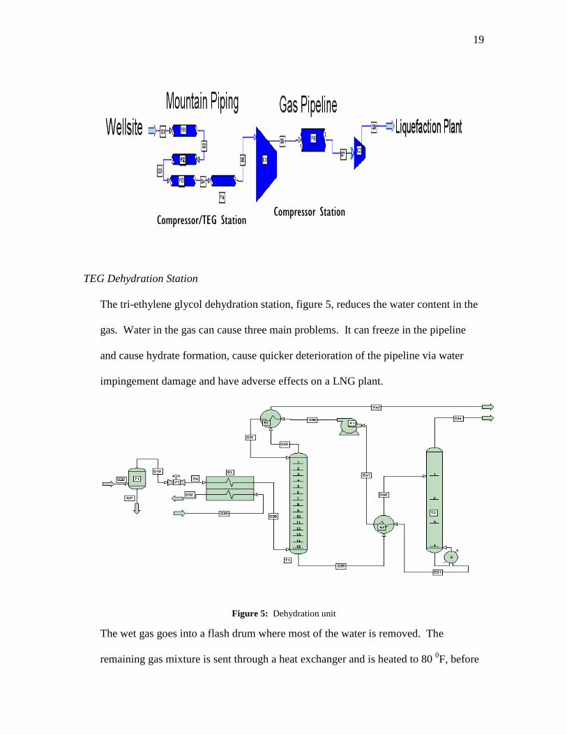
TEG Dehydration Station

The tri-ethylene glycol dehydration station, figure 5, reduces the water content in the

gas. Water in the gas can cause three main problems. It can freeze in the pipeline

and cause hydrate formation, cause quicker deterioration of the pipeline via water

impingement damage and have adverse effects on a LNG plant.

Figure 5: Dehydration unit

The wet gas goes into a flash drum where most of the water is removed. The

remaining gas mixture is sent through a heat exchanger and is heated to 80 0F, before

Compressor/TEG Station Compressor Station

20

going into an absorber and contacted with 90 0F TEG. The tri-ethylene glycol

collects the rest of the water from the gas mixture. The dry gas now heads out the top

of the absorber and is heated by a TEG stream before moving out to the large

compressor station. The water saturated TEG stream is then heated to 300F to enter

the still and is boiled at 380 0F to remove the water. The water now exits as steam out

the top of the still and dry TEG is recycled back to the absorber. The heat exchanger

cools the TEG to 90 0F before entering the absorber. The TEG dehydration plant was

simulated in ProII. The cost of the TEG dehydration station is expensive but is not a

major cost factor; the cost of the TEG dehydration station is calculated to be

$450,000.

Large Compressor Station

The large compressor station, figure 6, takes the gas from the dehydration unit,

and delivers it through 50 miles of 36” diameter pipe to the small compressor station.

The gas comes into the compressor station and is compressed through one of multiple

compressors before heading out to the pipeline.

Figure 6: Large compressor station

Multiple compressors allow one compressor to go offline for maintenance or repair

while the other compressors carry on full flow operations. Two methods of

21

calculating the work required by the compressors to feed a 50 mile pipeline are

estimated. The size of the pipe will be explained in the next section but assuming that

optimal pipe diameter is already decided upon, Bernoulli’s equation and a ProII

simulation are used to find the work required. Bernoulli’s method uses a spreadsheet

that optimizes pipe diameter with power requirements but does not account for

density changes in a gas through the pipeline. ProII’s simulation of the compressor

station gives reasonable data. The gas’ pressure increases to 2000kPa and

temperature increases to 5C. Bernoulli’s method gives a very small power

requirement of 6,300kW as compared to ProII’s value of 54,000kW. ProII’s realistic

power requirement is used. Each centrifugal–turbine–carbon steel compressor that is

used delivered 6,000kW of work with an individual cost of $3.6 million per 6,000kW

for a total cost of $33 million (Peters).

Pipeline

The pipeline extents for 49.7 miles but is rounded to 50 miles for calculating

purposes as seen in figure 7. The power requirements for the two compressor stations

are based upon the data selection for the pipe. Design considerations include a pipe

pressure that remains above reservoir pressure but below dew point pressure. A zero

change in height is assumed for the simulation but height changes can be added as the

project dictates.

22

Figure 7: Pipeline

There is no potential or kinetic energy losses assumed in the pipe, therefore the

energy loss becomes a function of change in pressure as shown in the following

equation (eqn. E).

∆

=∆

D

LfPf 1

22υρ

(Eqn. E)

Where:

f = fanning friction value

p = density

L = length

u = velocity

D = diameter

P = pressure

Since Bernoulli’s method does not give confident results, the results from ProII

are used. The lack of change in power requirements is attributed to the lack of

changing density data throughout the pipeline which would require a detailed

evaluation that is beyond the scope of this project. The final cost data proves to be a

close estimate of other cost estimates that are used, therefore no more time is spent on

this topic. For pipeline costs Bernoulli’s method is compared to Peters and

Timmerhaus online costing tutorial. Bernoulli’s method costs $20 million. Peters

23

and Timmerhaus give an extrapolated cost of $19 million (Peters). The costs are so

close that Bernoulli’s method is used for simplicity.

Small LNG Compressor Station

The pipeline before the LNG station is designed to achieve the necessary

temperature and pressure requirements for the LNG plant. The specifications are 5C

and 2000kPa. The power requirement of 560kW per compressor costing $300,000 is

a smaller requirement than the million dollar compressors at the large compressor

station.

Figure 8: Small compressor station

Pipeline Summary

The total pipe flowchart without the TEG dehydration station is shown below in

figure 9. The total capital investment will be $270 million. Wet methane produced

from the reservoir is sent to a TEG station where the water is removed. The dry gas

is then piped to a LNG station to be converted to liquid methane. Compressor

stations provide the driving force to meet pipeline pressure and temperature demands

24

of 15 °C and 2000 kPa to prevent reformation of hydrates and pipeline impingement

damage.

Figure 9: Pipeline flowchart

LNG Plant

The natural gas will be liquefied for shipping across the ocean. To do this a

simple cascade liquefaction plant was designed.

25

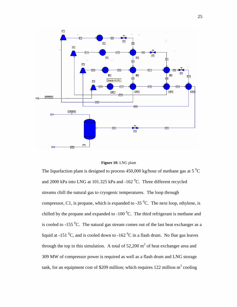
Figure 10: LNG plant

The liquefaction plant is designed to process 450,000 kg/hour of methane gas at 5 0C

and 2000 kPa into LNG at 101.325 kPa and -162 0C. Three different recycled

streams chill the natural gas to cryogenic temperatures. The loop through

compressor, C1, is propane, which is expanded to -35 0C. The next loop, ethylene, is

chilled by the propane and expanded to -100 0C. The third refrigerant is methane and

is cooled to -155 0C. The natural gas stream comes out of the last heat exchanger as a

liquid at -151 0C, and is cooled down to -162 0C in a flash drum. No flue gas leaves

through the top in this simulation. A total of 52,200 m2 of heat exchanger area and

309 MW of compressor power is required as well as a flash drum and LNG storage

tank, for an equipment cost of $209 million; which requires 122 million m3 cooling

26

water and 1.7 PW (1.7e9 kW) per year to operate. A total capital investment of

$1.25 billion is required to start-up this plant, with a total production cost of $270

million per annum or exactly $2.00 per MM Btu.

Delivery

Delivery consists of using three LNG ships to transport the gas from the LNG

plant on the coast of eastern Kamchatka to the country of Japan where a

Regasification plant is set up to receive the LNG and convert it to natural gas and

eventually sell it to the Japanese market. All the flow rates for the LNG and

Regasification plants are based on the capacity of three LNG ships divided by the

round trip and multiplied by a factor of 1.5. This allows the capacity of the plants,

pipeline and well to operate at 1.5 times the daily capacity rate of the LGN ship. This

should allow our equipment at various locations to perform in a safe operating range

of around 67%. This method makes the ship sort of like a back calculation. By

seeing what the capacity is of each ship and then optimizing the plants and pipeline to

handle 1.5 times that capacity, a cost value chain can be determined based on the

number of ships in operation. The average cost of an LNG ship that can hold 125,000

m^3 of LNG is $150,000,000. The data for the transit time and port docking days are

shown below in figure 11.

27

Calculations Data

Speed 15 nm/h Holding capacity 125,000.00 m3 of NGL

Distance Traveled 1480 nm volume flow rate 5,569.31 m3 per day (liquid)

Sea voyage time 4.11 days v (fluid) 422.62 kg/m3 liquid

Delays in voyage 4.11 days mass flow rate 2,353,700.50 kg/day (liquid)

Total one way sea voyage time 8.22 days molecular weight 16.043 g/mol

Pre & Post Dock days 6 days density (gas 1 atm, 15 C) 0.68 kg/m3

Total one way trip 11.22 days volumetric flow rate 3,461,324.26 scm/day (gas)

Total round way trip 22.44 days volumetric flow rate 122,243,588.80 scf/day (gas)

Cost of a one way trip $ 729,444.44 122 Million standard ft3 per day

Round trip Cost $1,458,888.89

Total daily cost $65,000.00

Table 1: Delivery

The sea voyage days calculated out to just over 4 days. But due to possible adverse

weather conditions in that area of the world the journey time was doubled to allow for

such harsh sailing conditions. Including the port days the total time for a round trip

came to just under 23 days. This estimate was massaged even more to allow for a

whole month to complete one round trip. The round trip cost of $1.5 million is a cost

function of the ship, financing charges and operating the ship. The prices vary quite

drastically from charter company to charter company but a good average of $65,000

per day was found (internet, February 1, 2006). Assumptions were made to calculate

total capital investment. Using the daily charter rate and a down payment cost, a

yearly budget could be determined over the 15 year contract with the charter

company. Based on the yearly budget, operational costs and yearly financing charges

could be determined. The down payment to the charter company is 5% of the total

ship cost. The finance charge comes out to 5.8% per year. The operational expenses

come to 52.1% per year.

28

Regasification Plant

The regasification plant is designed to heat up the LNG to a vapor of 40 0F before

being sold in the Japanese market. Seawater is used as the heat source, with propane

acting as the intermediate. For further study, water will be used as the heat source to

prevent corrosion problems with the heat exchangers. The plant is designed to

harness the cryogenic fluid’s heat capacity to generate power from fluid expansion in

the propane loop. This energy is captured by a turbine expander driving a generator

to produce usable energy (ESA Report, pg 3). The costs of including the propane

cycle save money over time, and produce a net electric utility of 53.5 TW per year.

In the future a design for capturing the expansion energy of LNG could also be added

to the Regasification plant design.

Figure 11: Regasification PFD

Pipeline to China

The high expense associated with building and operating the liquefaction plant

opens the door to explore other methods of transportation of the methane gas. A gas

pipeline, figure 13, to China starting from Kamchatka and running through eastern

Russia is explored as an alternative means of converting methane gas to LNG and

transporting via sea to the Japanese market. The gas pipeline to China extends

29

roughly 1700 miles. Varying diameters of piping from 30” to 36” are simulated in

ProII and priced according to Peters and Timmerhaus. The optimal diameter is 32”

and nine compressor stations. The pipeline is built with a pressure of 2000kPa and a

temperature of 15C as the operating conditions. With those conditions in mind, the

pipe length varies but the compressor stations remain rated for the most part at the

same horsepower. This method gives a very good evaluation of the compressor

power necessary to pipe the gas from Kamchatka to China. The total capital

investment for the gas pipeline is $2.6 billion which is much more expensive as

compared to the LNG process of $1.7 billion. The total production cost each year is a

different story though. The gas pipeline costs $186 million compared to the LNG

process of $ 445 million. The yearly operating cost of the LNG process is clearly

much more expensive than the gas pipeline yearly operating costs. But it is important

to remember that the LNG process has the flexibility to maneuver to differing

markets during times of change. In the case of China closing its doors to outsiders,

the gas pipeline could easily be lost and all the money invested in it gone.

30

Procedure Summary

The LNG is pumped from a storage tank via stream1. Heat is transferred from the

hot vapor propane to liquid natural gas. Heat is transferred to the gas and it comes

out of the heat exchanger at -30 0F. The propane is liquefied and goes into a pump to

be pumped to another heat exchanger where it will receive heat from the water. The

propane is again in a vapor form at 33 0F. As the propane is expanding, it is sent

through an expander where some of that expansion energy turns a turbine producing

shaft work to power a generator. The propane is then once again sent through the

LNG/propane heat exchanger and the cycle repeats. The natural gas from the

propane/LNG heat exchanger has not yet reached distribution temperatures and must

go through another heat exchanger, this time with seawater. The result is natural gas

at 40 0F ready to be piped to the Japanese market for sale. The specific data for the

Regasification plant can be seen in the spreadsheet in the appendix. The expander

31

produces enough power to drive all five pumps and still have power left over. The

most expensive cost is the storage tank unit. Its capacity is 160,000m^3. A normal

tank of this capacity would cost around $6 million; this one costs over $12 million.

The reason for the increase in cost is federal regulations that require the LNG tank to

be double hulled. It is required to have an outer shell, an inner shell and insulation

between the two shells. The inner shell is made of 9% nickel steel, the outer shell is

made of high-strength concrete and the insulation material is poly-urethane form

(PUF) (internet, March 1, 2006). Figure 13 below shows a few pictures of a LNG

storage tank (internet, March 1, 2006).

Figure 12: Storage Tanks

Recommendations

Liquefaction is the largest cost per MM Btu in the production cost. Alternatives

to the ConocoPhillips cascade will be explored, in order to find a cheaper way to

liquefy the natural gas.

32

The pipe has various density changes through its length which are not accounted

for in Bernoulli’s model or the ProII simulation. This can result in a large error and

cause a big cost fluctuation.

Delivery: Develop a cost model as a function of ship cost, financing and

operating expenses.

Regasification: Rigorous calculation of LNG storage tank. Efficiency values of

Heat exchangers, pumps, compressors and expanders. Simulate the conversion of

shaft work to generated electricity through the expander. Look into ways to harness

the expansion energy of the methane gas maybe by adding another propane reverse

refrigeration loop.

33

Works Cited

Chacin, Maria, Equilibrium and Non-Equilibrium Models Applied to Formation and Dissociation of Hydrates, 2005

Environmental and Social Action Report, January 2003

Foss, Michelle Michot, Introduction to LNG, 2003

http://www.eia.doe.gov/oiaf/analysispaper/global/lngindustry.html, February 1, 2006

http://www.osakagas.co.jp/rd/sheet/003e.htm, March 1, 2006

Jung, Yonghun , Economic Feasibility of Natural Gas Pipeline Projects in the Northeast Asia, 2002

Lombardi, Piero., Schlumberger

Mandil, Claude, The Global Outlook for LNG, 2004

Pereira, Sabata., Amerada Hess Corporation

Sloan, E. Dendy Jr., Clathrate Hydrates of Natural Gases, 1998