Unclassified ECO/WKP(2016)68 - OECD.org · Unclassified ECO/WKP(2016)68 Organisation de...

Unclassified ECO/WKP(2016)68 Organisation de Coopération et de Développement Économiques Organisation for Economic Co-operation and Development 25-Nov-2016

___________________________________________________________________________________________

_____________ English - Or. English ECONOMICS DEPARTMENT

THE EFFECT OF THE SIZE AND THE MIX OF PUBLIC SPENDING

ON GROWTH AND INEQUALITY

ECONOMICS DEPARTMENT WORKING PAPER No. 1344

By Jean-Marc Fournier and Åsa Johansson

OECD Working Papers should not be reported as representing the official views of the OECD or of its member

countries. The opinions expressed and arguments employed are those of the author(s).

Authorised for publication by Christian Kastrop, Director, Policy Studies Branch, Economics Department.

All Economics Department Working Papers are available at www.oecd.org/eco/workingpapers

JT03406188

Complete document available on OLIS in its original format

This document and any map included herein are without prejudice to the status of or sovereignty over any territory, to the delimitation of

international frontiers and boundaries and to the name of any territory, city or area.

EC

O/W

KP

(20

16)6

8

Un

classified

En

glish

- Or. E

ng

lish

Cancels & replaces the same document of 22 November 2016

ECO/WKP(2016)68

2

OECD Working Papers should not be reported as representing the official views of the OECD or of its member countries. The opinions expressed and arguments employed are those of the author(s).

Working Papers describe preliminary results or research in progress by the author(s) and are published to stimulate discussion on a broad range of issues on which the OECD works.

Comments on Working Papers are welcomed, and may be sent to OECD Economics Department, 2 rue André Pascal, 75775 Paris Cedex 16, France, or by e-mail to [email protected].

All Economics Department Working Papers are available at www.oecd.org/eco/workingpapers. This paper is part of an OECD project on the quality of public finance. Other outputs from this project include:

Fournier, J.M. (2016), “The Positive Effect of Public Investment on Potential Growth”, OECD Economics Department Working Papers, No. 1347, OECD Publishing,

Johansson, A. (2016), “Public Finance, Economic Growth and Inequality: A Survey of the Evidence”, OECD Economic Department Working Papers, No. 1346, OECD Publishing.

Bloch, D., J.M. Fournier, D. Gonzales and A. Pina (2016), “Trends in Public Finances: Insights from a New Detailed Dataset”, OECD Economic Department Working Papers, No. 1345, OECD Publishing.

This document and any map included herein are without prejudice to the status of or sovereignty over any territory, to the delimitation of international frontiers and boundaries and to the name of any territory, city or area. The statistical data for Israel are supplied by and under the responsibility of the relevant Israeli authorities. The use of such data by the OECD is without prejudice to the status of the Golan Heights, East Jerusalem and Israeli settlements in the West Bank under the terms of international law. Latvia was not an OECD Member at the time of preparation of this publication. Accordingly, Latvia does not appear in the list of OECD Members and is not included in the zone aggregates. © OECD (2016)

You can copy, download or print OECD content for your own use, and you can include excerpts from OECD publications, databases and multimedia products in your own documents, presentations, blogs, websites and teaching materials, provided that suitable acknowledgment of OECD as source and copyright owner is given. All requests for commercial use and translation rights should be submitted to [email protected]

ECO/WKP(2016)68

3

ABSTRACT/RÉSUMÉ

The effect of the size and the mix of public spending on growth and inequality

This paper provides evidence on the effects of the size and the composition of public spending on long-

term growth and inequality. An estimated baseline convergence model captures the long-term effect of

human capital and total investment on potential output for a panel of OECD countries. The composition of

public spending added to this baseline provides evidence that certain public spending items (public

investment and education) boost potential growth, while others (pensions and public subsidies) lower

potential growth. There is also evidence that too large governments reduce potential growth, unless the

functioning of government is highly effective. This paper also investigates the effect of public spending

items on income inequality. Increasing the size of government, family benefits or subsidies decreases

inequality. Reforms making the government more effective and an education reform that aims at

encouraging completion of secondary education may also decrease income inequality. Simulations

combining both growth and distributional effects illustrate that most reforms can deliver considerable

growth gains and benefit the poor.

JEL codes: H50; H52; H53; H54; H55; O40; D31

Keywords: Public spending, Government Size, Growth, Income inequality

*****

L’effet de la taille et de la composition des dépenses publiques sur la croissance et les inégalités.

Cet article fournit des preuves empiriques sur les effets de la taille et de la composition des dépenses

publiques sur la croissance à long terme et les inégalités. Un modèle de convergence de base mesure l’effet

à long terme du capital humain et de l’investissement total sur la production potentielle pour un panel de

pays de l’OCDE. La composition des dépenses publiques ajoutée à ce modèle de base montre que certains

postes de dépenses publiques (investissements publics et éducation) stimulent la croissance potentielle,

tandis que d’autres (pensions et subventions publiques) diminuent la croissance potentielle. Il est

également prouvé que des gouvernements trop importants réduisent la croissance potentielle, à moins que

le fonctionnement du gouvernement soit très efficace. Cet article examine également l’effet des dépenses

publiques sur les inégalités de revenus. Augmenter la taille du gouvernement, les prestations familiales ou

les subventions diminue les inégalités. Les réformes rendant le gouvernement plus efficace et une réforme

de l’éducation qui vise à encourager l’achèvement de l’enseignement secondaire peuvent également réduire

les inégalités de revenus. Des simulations combinant les effets de croissance et de distribution montrent

que la plupart des réformes peuvent générer des gains de croissance considérables et bénéficier aux

pauvres.

Codes JEL : H50 ; H52 ; H53 ; H54 ; H55 ; O40 ; D31

Mots clés : Dépenses publiques, Taille du Gouvernement, Croissance, Inégalités de Revenu

ECO/WKP(2016)68

4

TABLE OF CONTENTS

1. Introduction and main findings ............................................................................................................. 6 2. Related literature ................................................................................................................................... 8

2.1. Public spending and economic growth .............................................................................................. 8 2.2. Public finance and income distribution ............................................................................................. 9

3. Data ....................................................................................................................................................... 9 3.1. Breakdown of public expenditure ..................................................................................................... 9 3.2. Income distribution data .................................................................................................................. 11 3.3. Other variables ................................................................................................................................ 12

4. Empirical set up .................................................................................................................................. 12 4.1. Framework ...................................................................................................................................... 12 4.2. Public spending and growth ............................................................................................................ 13 4.3. Public spending and inequality ........................................................................................................ 16

5. Estimation results................................................................................................................................ 17 5.1. The baseline growth results ............................................................................................................. 17 5.2. The effect of public spending on growth ......................................................................................... 19 5.3. The direct effect of public spending on inequality .......................................................................... 27

6. Simulations of growth and inequality effects of public spending reforms ......................................... 31 6.1. Illustrative growth gains .................................................................................................................. 31 6.2. Illustrative disposable income effects ............................................................................................. 35

7. Conclusion ............................................................................................................................................. 37

REFERENCES .............................................................................................................................................. 38

ANNEX 1 ...................................................................................................................................................... 42

Tables

1. The main effects of public spending reforms on growth and inequality ....................................... 7

2. The public expenditure breakdown ............................................................................................. 10

3. Correlation between public spending items and country-specific features ................................. 15

4. Most of the variability of the public spending structure is across countries................................ 15

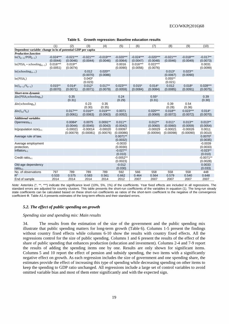
5. Growth regression: Baseline education results ............................................................................ 19

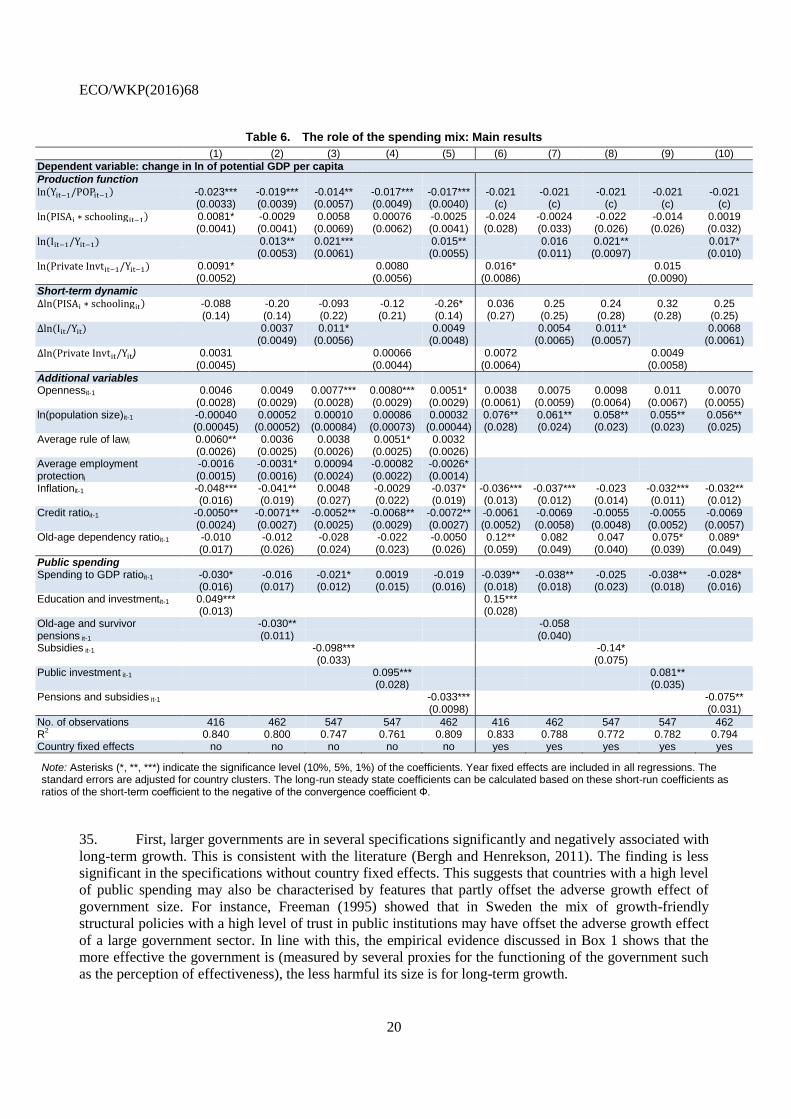
6. The role of the spending mix: Main results ................................................................................. 20

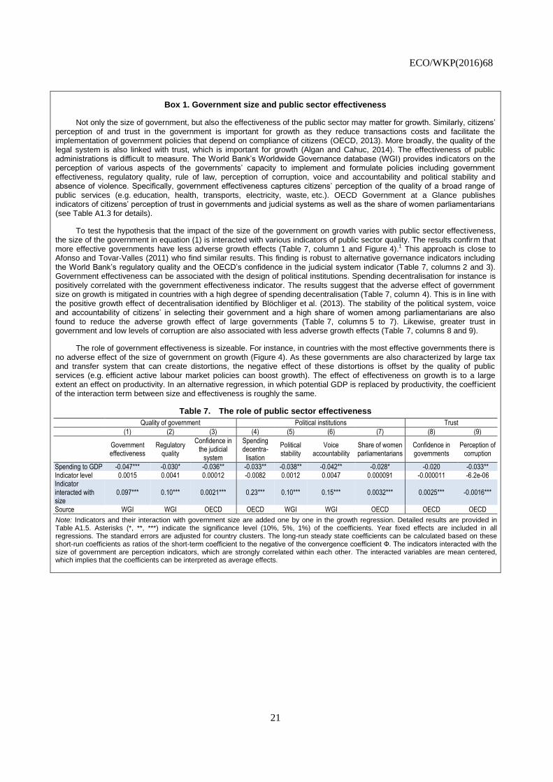
7. The role of public sector effectiveness ........................................................................................ 21

8. The effect of government size and public investment on the speed of convergence ................... 27

A1.1. Public spending breakdown ......................................................................................................... 42

A1.2. The composition of public primary spending by country ............................................................ 43

A1.3. Data definitions ........................................................................................................................... 44

A1.4. Growth regression: Baseline results, long-term effects ............................................................... 46

A1.5. The role of public sector effectiveness ........................................................................................ 47

A1.6. The effect of government size and public investment on the speed of convergence ................... 48

ECO/WKP(2016)68

5

A1.7. The role of the spending mix: Spending items as GDP shares .................................................... 49

A1.8. The role of the spending mix: Pre-crisis estimates ...................................................................... 50

A1.9. The role of the spending mix: Spending items with two lags...................................................... 51

Figures

1. Data imputation ........................................................................................................................... 10

2. Structure of spending ................................................................................................................... 11

3. A simple framework to encompass growth and inequality effects .............................................. 13

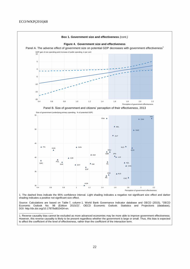
4. Government size and effectiveness ............................................................................................. 22

5. Estimates of decreasing returns to public investment.................................................................. 26

6. Larger governments reduce inequality ........................................................................................ 28

7. More effective governments are beneficial for the poor ............................................................. 29

8. Increasing attainments in secondary education decreases inequality .......................................... 30

9. Some spending items matter for inequality ................................................................................. 31

10. Potential long-term growth effect of an increase in the education level ..................................... 32

11. Potential long-term growth effect of a change in the public spending mix ................................. 33

12. Potential GDP gains from reducing the size and improving the effectiveness

of the government ........................................................................................................................ 34

13. Potential gains from reducing the size of the government along the income distribution ........... 36

14. Potential gains from changing the spending structure along the income distribution ................. 37

A1.1. Direct effects by disposable income decile ................................................................................. 52

A1.2. Larger and more effective governments do not change market income inequality ..................... 53

A1.3. Some spending items matter for inequality: Spending items as GDP shares .............................. 54

Boxes

Box 1. Government size and public sector effectiveness ........................................................................... 21

Box 2. Decreasing returns to public investment ........................................................................................ 25

ECO/WKP(2016)68

6

THE EFFECT OF THE SIZE AND THE MIX OF PUBLIC SPENDING

ON GROWTH AND INEQUALITY

By Jean-Marc Fournier and Åsa Johansson1

1. Introduction and main findings

1. Governments in the OECD spend on average about 40% of GDP on the provision of public

goods, services and transfers. The sheer size of the public sector has prompted a large amount of research

on the link between the size of government and economic growth (see Bergh and Henrekson, 2011 for an

overview). Much less is known about the composition of spending for long-term growth and inequality.

Reflecting differences in policy objectives, the provision of public services including the degree of

redistribution differs considerably among countries. In turn, the composition of spending and its design can

have repercussions for growth and the distribution of income. This paper shows that cross-country

differences in the size and the composition of spending can potentially explain sizeable differences in the

level and distribution of income.

2. This paper investigates empirically the effect of the size and the composition of public spending

on long-term growth and disposable income inequality in OECD countries. The estimation of the effect of

public spending on growth builds on the recent empirical literature on the determinants of long-term

growth (e.g. Barro, 2015). The impact of public spending on income distribution encompasses two effects:

a direct effect on the distribution of household disposable income and an indirect effect via growth. The

estimation of the direct impact of public spending along the income distribution follows Hermansen et al.

(2016). The overall effect of public finance on household disposable income adds the growth effect to the

direct effect on the distribution of income.

3. In the analysis, the composition effect of public spending is disentangled from the size effect.

The overall financing need is not affected by a change in the spending composition. This allows

disregarding the distortionary effects of taxation when assessing the specific effect of each spending item.

To analyse the effect of public spending, the paper relies on a newly constructed dataset on public

spending across OECD countries, which combines various existing data sources in a consistent manner

(Bloch et al., 2016). Various breakdowns of spending into detailed items are considered in the empirical

analysis. The set-up in this paper allows highlighting potential trade-offs between growth and inequality.

1. The authors are members of the Economics Department of the OECD. They thank OECD Economics

Department colleagues Falilou Fall, Peter Gal, Peter Hoeller, Catherine Mann and Jean-Luc Schneider for

comments and suggestions. The paper has also benefitted from comments by members of Working Party

No. 1 of the OECD Economic Policy Committee. Special thanks go to Debra Bloch for statistical

assistance and Celia Rutkoski (also from the Economics Department) for assistance in preparing this

document.

ECO/WKP(2016)68

7

4. The main findings that emerge from the analysis are (see Table 1 for a summary):

On the size and effectiveness of government

Larger governments are associated with lower long-term growth. Larger governments also slow-

down the catch-up to the productivity frontier.

The adverse growth effect of large governments can be offset, if countries have well-functioning

governments (e.g. the Nordic countries). A high degree of spending decentralisation also

mitigates the adverse growth effect of large governments.

In the countries with the most effective governments, the large size of the government promotes

equity with no adverse effect on growth. This likely reflects that larger governments tend to

redistribute more, and that better functioning governments tend to better target transfer

programmes to disadvantaged groups.

In countries with less effective governments, improving government effectiveness can both

increase growth and reduce inequality. In these countries, reducing the size of government

increases income of all. Nonetheless, it benefits less those with lower income as smaller

governments tend to redistribute less.

Table 1. The main effects of public spending reforms on growth and inequality

Policy Growth Equity Income of the poor

Countries with the most room for growth gains

Decreasing the size of government

Low to moderate government effectiveness

+ - + BEL, CZE, FRA, GRC,

HUN, ITA, POL, PRT, SVN High government effectiveness

n.s. - -

Increasing government effectiveness + + + FRA, GRC, HUN, ITA, SVN

Increasing education outcomes + 0/+ + CHL, GRC, MEX, PRT, TUR

Increasing public investment (including R&D) + n.s. + BEL, DEU, GBR, IRL, ISR, ITA, MEX, TUR

Pension reform + n.s. + AUT, DEU, FIN, FRA, GRC, ITA, JPN, POL, PRT, SVN

Increasing family benefits n.s. + + CHE, ESP, GRC, PRT

Decreasing public subsidies + - n.s. BEL, CHE

Note: + stands for a positively significant, – for a negatively significant and n.s. for non-significant effect. For instance, a decrease in the size of the government (at low to moderate levels of government effectiveness) increases growth, while it reduces equity. The 0/+ indicates that the equity effect of education depends on whether the reform focuses on reducing inequality in educational attainment or not. The countries with most room for growth gains are those where reforms would yield gains of more than 10% of GDP. For family benefits, the table shows countries where the reform would increase the income of the poor by more than 20%. Details of these reforms are discussed in section 6.

On the structure of spending

For a given level of public education spending, improving student performance yields large gains

for all by raising skills and thereby productivity. An education reform that aims at encouraging

completion of secondary education may also decrease income inequality as it can reduce

education inequality.

Increasing the share of public investment in spending yields large growth gains. These gains are

particularly strong for public investment in health (e.g. hospitals and their equipment). A

spending shift towards public investment, away from other spending, would also speed up the

ECO/WKP(2016)68

8

convergence of income towards the most advanced economies. Overall, such a spending shift

would lift “all boats” as it raises average income without any adverse equity effect.

The growth gains from increasing public investment may decline at a high level of the public

capital stock due to decreasing returns. Still, the estimations suggest that all OECD countries,

except Japan, have room for additional public investment.

Reducing the share of pension spending in primary spending yields sizeable growth gains with

no significant adverse effect on disposable income inequality. This reduction could be achieved

by an increase in the effective retirement age or by cutting the replacement rate. However, cutting

pensions entails a trade-off between the old and the young.

Cutting public subsidies boosts growth, as public subsidies that do not correct market failures can

distort the allocation of resources and undermine competition. But this reform would increase

inequality as cutting subsidies delivers large disposable income gains for the rich and no gains for

the poor. This is because the growth-enhancing effect of a reduction of subsidies on the income

of the poor compensates the adverse equity effect via less redistribution.

A shift in spending towards family benefits and child care, away from other spending, reduces

disposable income inequality as these benefits tend to be worth comparatively more for lower-

income families. They may also facilitate the participation of second earners in the labour market.

2. Related literature

2.1. Public spending and economic growth

5. This paper tackles the question of how to design public spending to promote inclusive growth. To

address this question it builds on the empirical public finance literature analysing the effect of fiscal policy

on long-term growth (e.g. Myles, 2009 and Johansson, 2016 for an overview). There is a vast empirical

literature investigating the relationship between the size of the government and economic growth (see

Slemrod, 1995; Myles 2009; Bergh and Henrekson, 2011 for overviews). A review by Bergh and

Henrekson (2011), based on papers published in peer reviewed journals after 2000, suggested a negative

relationship in OECD countries. Likewise, a recent OECD study confirmed a negative relationship

between the size of government and GDP growth (Fall and Fournier, 2015). The direction of the link

between the size of government and growth may vary with the income level and could be hump-shaped

(Armey, 1995). A few studies have found support for the existence of a non-linear relationship between the

size of government and growth (e.g. Vedder and Gallaway, 1998; Pevcin, 2004; Chen and Lee, 2005). Yet,

it is important to keep in mind that a negative correlation does not imply causality. In the short run, in

particular when some government spending is constrained by past commitments, a negative correlation

between the share of government spending and current growth is expected. Another possible cause of

reverse causality is that in developing countries it is more difficult to extract government revenue, which

constrains the size of government.

6. Cross-country empirical studies estimating the impact of the structure of spending on growth

generally provides evidence that the mix of spending matters for growth. Often these papers classify

government spending into productive and non-productive spending, depending on whether they are

included in the production function or not (e.g. Barro, 1990). For instance, investment in infrastructure and

education can raise the human and physical capital stock and, in turn, long-run growth. Since Kneller et al.

(1999), a number of papers found that productive spending affects economic growth positively, while

unproductive spending does not. One of the key insights of Kneller et al. (1999) is the importance of

controlling for the government’s budget constraint as failing to do so would yield biased estimates. Recent

studies consider this constraint by controlling for the size of government, which is also the strategy used in

this paper. For instance, Teles and Mussolini (2014) found in a sample of developing and developed

ECO/WKP(2016)68

9

countries, that productive spending affects economic growth positively, though this impact declines as

public debt increases. Gemmell et al. (2014) focused on the long-run GDP impact of changes in total

government spending and in the shares of different spending categories in total spending in OECD

countries. Their results imply that reallocating total spending towards infrastructure and education would

raise income in the long run.2 Increasing the share of social welfare spending is associated with modestly

lower long-run GDP levels.

2.2. Public finance and income distribution

7. Apart from affecting growth, the size and the composition of public spending can also influence

household disposable income. Public spending, such as on unemployment and welfare support, directly

affects income (e.g. Joumard et al., 2012). Public spending can also influence household income indirectly

via its impact on GDP per capita. Recent OECD research investigated how gains in long-term GDP per

capita “trickle down” to households along the income distribution (Causa et al., 2014a). This opens up

another channel through which public spending can affect inequality.

8. There is a growing empirical literature investigating the effects of various social spending items

on measures of inequality (i.e. labour earnings or disposable income inequality). Förster and Toth (2015)

provide an overview of cross-country studies on causes of income inequality that covers the role of taxes

and transfers. There is some empirical support for the inequality reducing effect of unemployment benefits

(Koeniger et al., 2007; Causa et al., 2014b for unemployment benefits to long-term unemployed).

Likewise, there is also some evidence that when active labour market programmes increase jobseekers’

employment chances and wages once in employment, they reduce income inequality (Salverda and

Checchi, 2014; Causa et al., 2014b). Other research has shown that public employment can decrease

inequality (Fournier and Koske, 2012). For example, when there is no political support for tax and transfer

reforms policy makers may use public employment as a redistributive tool (Alesina et al., 2000).

3. Data

3.1. Breakdown of public expenditure

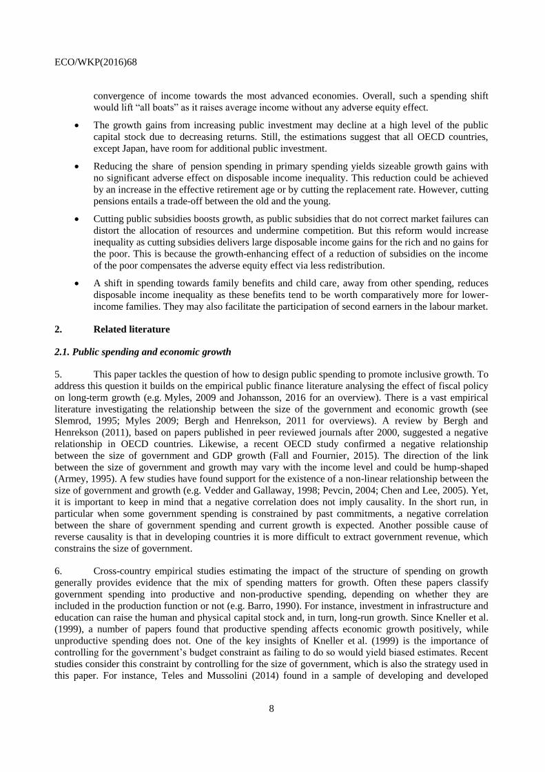
9. Public expenditure is classified into 10 primary expenditure items plus interest payments

(Table 2). This breakdown is motivated by the potential impact of different public expenditure items on

growth and inequality and is similar to the one considered in Cournède et al. (2013). Based on growth

theory, the breakdown makes a distinction between public spending that provides a production input, such

as education or physical investment, and other current expenditure such as social transfers. The items do

not overlap. For instance, physical investment in education, such as building a new school, is included in

the public investment item. It is not included in the education item that focuses on current education

spending. Expenditure functions that are not reported here (e.g. defence, justice) are mainly included in the

item “Other wages and intermediate consumption” and in the investment item. More details on the

breakdown are presented in Table A1.1.

2. Hanushek and Woessmann (2012) find a strong impact of cognitive skills on growth. However, research

tends to show only a weak relationship between the amount of educational spending and student

performance (e.g. PISA scores) (Hanushek and Woessmann, 2011). Thus, policies aiming at increasing

education spending effectiveness are likely to be more effective in improving education outcomes and

hence growth than increases in education spending.

ECO/WKP(2016)68

10

Table 2. The public expenditure breakdown

Item Label Comments

1 Education Includes wages, intermediate consumptions and transfers 2 Health Includes wages, intermediate consumptions and transfers 3 Other wages and intermediate consumption Wages and intermediate consumption that are not in items 1, 2, 5 and 7

4 Old-age and survivor pensions Includes transfers only 5 Sickness and disability Includes wages, intermediate consumptions and transfers 6 Unemployment benefits Includes transfers only 7 Family and children Includes wages, intermediate consumptions and transfers 8 Subsidies 9 Investment

10 Other primary expenditure Includes capital transfers and other elements 11 Interest payments

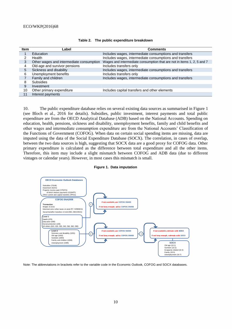
10. The public expenditure database relies on several existing data sources as summarised in Figure 1

(see Bloch et al., 2016 for details). Subsidies, public investment, interest payments and total public

expenditure are from the OECD Analytical Database (ADB) based on the National Accounts. Spending on

education, health, pensions, sickness and disability, unemployment benefits, family and child benefits and

other wages and intermediate consumption expenditure are from the National Accounts’ Classification of

the Functions of Government (COFOG). When data on certain social spending items are missing, data are

imputed using the data of the Social Expenditure Database (SOCX). The correlation, in cases of overlap,

between the two data sources is high, suggesting that SOCX data are a good proxy for COFOG data. Other

primary expenditure is calculated as the difference between total expenditure and all the other items.

Therefore, this item may include a slight mismatch between COFOG and ADB data (due to different

vintages or calendar years). However, in most cases this mismatch is small.

Figure 1. Data imputation

Note: The abbreviations in brackets refer to the variable code in the Economic Outlook, COFOG and SOCX databases.

Subsidies (TSUB)

Investment (IGAA)

Level 2

Sickness and disability (1001)

Old age (1002)

Survivors (1003)

Family and children (1004)

Unemployment (1005)

Old age (10.1)

Survivors (10.2)

Incapacity related (10.3)

Family (10.5)

Unemployment (10.7)

Education (090)

Social protection (100)

All others (010, 020, 030, 040, 050, 060, 080)

if not available,use COFOG SNA93

if not long enough, estimate with SOCX

Intermed.cons+other taxes on prod (P2_D29D8CG)

Social benefits+transfers in kind (D62_D631XXCG)

Level 1

Health (070)

SOCX

Other current and capital transfers (TPKG)

Property income paid (YPEPG)

of which Interest payments (GGINTP)

OECD Economic Outlook Databases

COFOG SNA2008if not available,use COFOG SNA93

Transaction

Wages (C1CG) if not long enough, splice COFOG SNA93

if not available,estimate with SOCX

if not long enough, splice COFOG SNA93

1

2 3

ECO/WKP(2016)68

11

11. Certain public expenditure items are sensitive to the business cycle. To obtain a measure of

structural expenditure, unemployment benefits, other income related transfers and capital transfers are

cyclically-adjusted following the methodology of Price et al. (2015). The other spending items are not

cyclically-adjusted as their sensitivity to the cycle is limited (e.g. public investment is not cyclically-

adjusted as its variation reflects discretionary choices, rather than automatic stabilisers). In order to focus

on long-term structural effects, the spending items are expressed as ratios to potential GDP.

12. Relying on this database shows that on average across OECD countries the bulk of spending is on

social protection such as old-age and survivors pension, sickness and disability, unemployment benefits

and family and child care benefits. Combined they account on average for about 35% of primary public

spending. Education spending and public investment account together on average for some 18% and health

spending for on average around 15% of primary spending (Figure 2). Over the past decade, the level and

the structure of spending have remained fairly stable. These averages mask considerable cross-country

differences (see Bloch et al. 2016 for details).

Figure 2. Structure of spending

Average across OECD countries, % of potential GDP

Note: Unweighted average of 27 OECD countries. The average for 2013 includes data for 2012 for Israel and the United States. The figure shows cyclically-adjusted spending items. A public spending breakdown by country is reported in Table A1.2.

Source: Forthcoming public finance dataset as documented in Bloch D., J.M. Fournier, D. Gonzales and A. Pina (2016), “Trends in Public Finances: Insights from a New Detailed Dataset”, OECD Economic Department Working Paper, No. 1345, OECD Publishing, Paris.

3.2. Income distribution data

13. The measure of inequality is based on the distribution of household disposable income for the

total population. The source is the OECD Income Distribution database, which combines household survey

data into semi-aggregated data (i.e. disposable income by decile). Household disposable income includes

labour income (wages, salaries and self-employment income), capital income and net government transfers

(cash transfers net of direct taxes paid by households). In-kind transfers, such as for health and education,

could not be included as it is not possible to allocate these transfers to the individuals observed in the

household survey data.

Public investment Public investment Public investment

Education EducationEducation

HealthHealth

Health

Old-age and survivor pensions



Sickness and disabilitySickness and disability Sickness and disabilityUnemployment benefits

Unemployment benefits Unemployment benefitsFamily and child

Family and child Family and child

Wages and intermediate

consumption - other purposes





Subsidies

SubsidiesSubsidies

Other primary expenditure



0

5

10

15

20

25

30

35

40

45

2001 2007 2013

Per cent of potential GDP

ECO/WKP(2016)68

12

3.3. Other variables

14. The OECD Economic Outlook November 2015 database is the source for the macroeconomic

variables (see Table A1.3 for details). The quality of education is measured as the average of reading,

science and math PISA scores in 2006.3 This is a proxy for the quality of education since in most countries

average PISA scores have remained fairly stable over time. The source of average years of schooling of the

working-age population is the OECD Long-term Economic Outlook database. The rule of law indicator is

from the Worldwide Governance Indicator (WGI) database of the World Bank. Employment protection

legislation (EPL) is the protection for regular contracts based on the second edition of this OECD indicator.

For these two slow-moving indicators, the average value over the available years is used in the

regressions.4 The stock of public capital is from the IMF’s Investment and Capital Stock Dataset. The

credit to GDP ratio is from the World Bank Global Financial Development database, with some

adjustments made as in Cournède and Denk (2015).

15. The final baseline sample for the growth regressions covers 789 country-year observations over

1987-2014, where the main restriction for the coverage of the sample is the availability of cyclically-

adjusted data. When including all spending items, the sample size shrinks to 416. The inequality analysis

covers 202 country-year observations over 1988-2012 with a biennial frequency. Data availability in the

OECD Income Distribution database is limited in the early years so that observations before 2000 could be

used in about half of the countries.5

4. Empirical set up

4.1. Framework

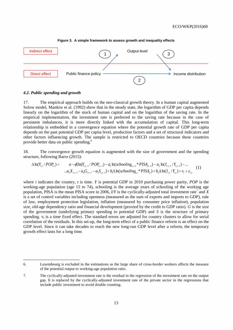
16. The effects of public spending on growth and inequality are estimated separately. First, the

estimates of the impact of the size and the composition of public spending on GDP per capita draw on the

standard convergence model (Barro (2015), first arrow in Figure 3). Second, estimates of the direct impact

of different public spending items along the income distribution (second arrow in Figure 3) follow

Hermansen et al. (2016). The empirical approach in this paper disentangles the direct effect of a public

spending reform on the income distribution from the effect of this reform on GDP per capita by controlling

for GDP per capita (e.g. Causa et al., 2014a). Therefore, the effect of public finance on growth is combined

with the effect of growth on disposable income (third arrow in Figure 3). The overall effect of public

finance on the distribution of disposable income is the sum of the direct effect on disposable income and

the indirect growth effect.

3. The year 2006 is chosen because it is the earliest PISA vintage in which the science performance scale is

the same as the one used in the following vintages (OECD, 2014). In the case of the United States, the

2009 average is used as the 2006 reading score is not available.

4. Replacing the average rule of law with the time-varying indicator yields broadly unchanged results

(assuming that the index pre-1996 is equal to the value in 1996).

5. Some countries only provide data at five-year intervals up to the mid-2000s. In countries where other

sources confirm the underlying development in inequality, linear interpolation is used to fill in the data for

missing years.

ECO/WKP(2016)68

13

Figure 3. A simple framework to assess growth and inequality effects

4.2. Public spending and growth

17. The empirical approach builds on the neo-classical growth theory. In a human capital augmented

Solow model, Mankiw et al. (1992) show that in the steady state, the logarithm of GDP per capita depends

linearly on the logarithm of the stock of human capital and on the logarithm of the saving rate. In the

empirical implementation, the investment rate is preferred to the saving rate because in the case of

persistent imbalances, it is more directly linked with the accumulation of capital. This long-term

relationship is embedded in a convergence equation where the potential growth rate of GDP per capita

depends on the past potential GDP per capita level, production factors and a set of structural indicators and

other factors influencing growth. The sample is restricted to OECD countries because these countries

provide better data on public spending.6

18. The convergence growth equation is augmented with the size of government and the spending

structure, following Barro (2015):

tittititititititi

titititititititi

vYIbPISAschoolingbSaGaXa

YIaPISAschoolingaPOPYaPOPY

,,,2,,11,51,41,3

1,1,21,1,11,1,,,

)/ln()*ln(]...

...)/ln()*ln()/[ln()/ln(

(1)

where i indicates the country, t is time. Y is potential GDP in 2010 purchasing power parity, POP is the

working-age population (age 15 to 74), schooling is the average years of schooling of the working age

population, PISA is the mean PISA score in 2006, I/Y is the cyclically-adjusted total investment rate7 and X

is a set of control variables including openness (measured as the sum of exports and imports to GDP), rule

of law, employment protection legislation, inflation (measured by consumer price inflation), population

size, old-age dependency ratio and financial development (proxied by the credit to GDP ratio). G is the size

of the government (underlying primary spending to potential GDP) and S is the structure of primary

spending. vt is a time fixed effect. The standard errors are adjusted for country clusters to allow for serial

correlation of the residuals. In this set-up, the long-term effect of a public finance reform is an effect on the

GDP level. Since it can take decades to reach the new long-run GDP level after a reform, the temporary

growth effect lasts for a long time.

6. Luxembourg is excluded in the estimations as the large share of cross-border workers affects the measure

of the potential output to working-age population ratio.

7. The cyclically-adjusted investment rate is the residual in the regression of the investment rate on the output

gap. It is replaced by the cyclically-adjusted investment rate of the private sector in the regressions that

include public investment to avoid double counting.

Public finance policy

Output level

Income distribution

1

2

3Indirect effect

Direct effect

ECO/WKP(2016)68

14

19. Following the recent literature, the specification controls for the size of government to account

for the government’s budget constraint (e.g. Arnold et al., 2011a; Gemmell et al., 2014).8 The structure of

spending is captured by the detailed spending breakdown outlined in Table 2. The spending items are

measured by the spending shares of different spending items in total spending excluding interest payments

(or GDP in a robustness check). To avoid collinearity, one (or a group) of the spending items is omitted in

the estimation.

20. The estimation strategy follows closely Barro (2015) to ensure that the estimation of the

convergence coefficient is unbiased. In this paper, the convergence coefficient is estimated with an

ordinary least square estimator with year fixed effects. Country fixed effects are not included because with

a small time dimension, Nickell (1981) and Arellano and Bond (1991) show that there is a Hurwicz

(1950)-type bias of the estimated coefficient for the convergence term. This bias is much larger than the

convergence coefficient itself according to Nickell's (1981) formula and Barro's (2015) estimates.

Furthermore, Nerlove (2000) also underlines that the bias of the convergence term will affect the estimates

of the coefficients of all variables that are correlated with the level of GDP. Without country fixed effects,

the model captures a convergence process conditional only on the control variables. Therefore, countries

converge to the productivity frontier if these control variables converge to those of the country at the

technology frontier.

21. Once the convergence coefficient is estimated, two different methods are used to estimate the

effect of the size and the structure of public spending on GDP per capita. The first approach is the ordinary

least square estimator with year fixed effects, but without country fixed effects. This approach assumes that

the omitted variable bias is small when a large set of control variables is included. The second approach

adds country fixed effects and the convergence coefficient is constrained to be equal to the one estimated

in the regression without country fixed effects. This second option has the advantage that it controls for

unobserved country-specific characteristics while circumventing the risk of a Hurwicz-type bias for the

convergence coefficient.

22. Several checks confirm that the omitted variable bias in the specification without fixed effects is

much smaller than the convergence bias. For most spending items, the correlation between the public

spending mix and important country-specific characteristics is low (Table 3). The specification includes a

large set of controls, including the rule of law and the employment protection legislation (EPL) that show

the strongest correlation with the public finance mix. Moreover, the comparison of the coefficient

estimates without and with fixed effects reveals that the omitted variable bias is not a major issue.

8. Alternative regressions in which government spending is replaced by two variables, the sum of the

remaining items and the primary balance, assumes that the reform is funded by a tax increase. Such

regressions provide similar results for spending item effects. Hence, the way the spending reform is

financed does not seem not to matter.

ECO/WKP(2016)68

15

Table 3. Correlation between public spending items and country-specific features

Variable Rule

of law Years of schooling

Average PISA

Employment protection

Credit ratio

Stock market ratio

Product market

regulation

State control (PMR)

Public spending size 0.23 -0.08 -0.19 0.42 -0.07 -0.24 -0.14 0.04 Education 0.04 -0.17 0.03 -0.34 0.13 0.15 0.08 -0.02 Health 0.14 0.02 -0.14 -0.18 0.36 -0.11 -0.30 -0.35 Other wages and intermediate consumption -0.27 0.16 -0.16 -0.29 -0.10 0.04 0.12 -0.07 Old-age and survivor pensions -0.30 -0.22 -0.06 0.39 -0.07 -0.12 0.08 0.28 Sickness and Disability 0.40 0.22 0.03 -0.10 -0.09 0.12 -0.09 -0.13 Unemployment benefits 0.36 -0.07 0.19 0.16 0.04 -0.06 -0.03 0.02 Family and children 0.48 0.16 -0.02 -0.24 0.02 -0.02 -0.28 -0.27 Subsidies 0.29 0.06 0.08 0.17 -0.05 0.18 0.09 0.14 Public investment -0.25 -0.11 0.34 -0.17 0.03 0.01 0.22 0.05 Other primary expenditure -0.13 0.18 -0.05 -0.04 -0.12 0.08 0.12 -0.01

Note: Expenditure items are measured as shares of primary spending.

Source: OECD calculations built on sources listed in Table A1.3.

23. The specification without country fixed effects also captures the impact of fundamental cross-

country differences in the design of public finance on growth. Most public finance variables vary only

slowly over time within a country, while cross-country heterogeneity is much larger (Table 4). For

instance, the estimated coefficient of a spending item in the growth equation may capture key structural

differences in the provision of public services across countries such as a persistently low share of spending

on social protection in Korea and the United States. As the specification without country fixed effects

exploits both the cross- and within country variability, the standard errors of the coefficient estimates are

lower.

Table 4. Most of the variability of the public spending structure is across countries

Item no. Variable Share of between country variance in total variance

1 Education 92%

2 Health 83%

3 Other wages and intermediate consumption 84%

4 Old-age and survivor pensions 92%

5 Sickness and disability benefits and services 87%

6 Unemployment benefits 85%

7 Family and child benefits and services 92%

8 Subsidies 81%

9 Public investment 77%

10 Other primary expenditure 91%

Note: Expenditure items are measured as shares of primary spending.

Source: Forthcoming public finance dataset as documented in Bloch D., J.M. Fournier, D. Gonzales and A. Pina (2016), “Trends in Public Finances: Insights from a New Detailed Dataset”, OECD Economic Department Working Paper, No. 1345, OECD Publishing, Paris.

24. A priori estimates with ordinary least squares can capture the causality in both directions.

Business cycle effects and Wagner’s law (the tendency for government expenditure to be larger at higher

levels of per capita GDP) are the most likely source of endogeneity in growth regressions including the

effect of the size of government (Easterly and Rebelo, 1993; Kneller et al., 1999). The use of cyclically-

ECO/WKP(2016)68

16

adjusted GDP data should attenuate the effect of short-term GDP fluctuations on the government size and

spending mix.9 Wagner’s law posits that higher income results in increasing political pressure for social

programmes. This should create a positive link between the size of the government and growth, going

against the negative effect of government size found in this paper: the adverse effect of government size

and the share of social spending on growth could be underestimated. As OECD countries have reached

quite comparable levels of development, it is likely that Wagner’s law plays a secondary role in shaping

the link between government size and spending composition and GDP.10

In sum, the reverse causality bias

is likely to be small.

4.3. Public spending and inequality

25. Public finance influences household disposable income in two ways: (i) directly by affecting

household income; and (ii) indirectly via its impact on GDP per capita (see the previous section). The

estimation in equation (2) below provides the direct effect of the structure of public finance on inequality.

Specifically, the estimated equation follows Hermansen et al. (2016):

]lnln)([lnln*))(ln( ,,1,41,31,21,11,,2,,1, tititititititititi SGNEGDPxGDPx (2)

where tix ,)( is an income level indicator that captures a part of the distribution of income, such as the

general mean or the decile for time period t and country i. The lagged level of this indicator controls for

income convergence. GDP is GDP per capita, Δln𝐺𝐷𝑃𝑖𝑡 is GDP per capita growth, and NE𝑖𝑡 is the net

export to GDP ratio. Net export controls for the fact that the mean household income elasticity to GDP is

likely to deviate from one in open economies with persistent external imbalances as these can be associated

with a gap between production and household income growth. Results are robust if net exports are replaced

by the terms-of-trade, which captures relative price differences that can create a gap between GDP and

household income. 𝛾𝑡 denotes time controls and 𝜂𝑖 denotes country fixed effects.

26. Similarly to the growth regressions, the various spending items (S) in Table 2 are added to the

specification controlling for the size of public spending (G). Since the specification controls for GDP per

capita, the estimated effect of the size and the structure of public finance in equation (2) should be

interpreted as the direct effect on the distribution of income. The overall effect of public finance on

household income is obtained by adding the indirect (i.e. the effect of a change in public finance

channelled via a change in GDP per capita as estimated in equation (1)) to the direct effect. The coefficient

4 captures the direct effect of the spending mix on the distribution of household income and 1 the effect

of GDP per capita on the distribution of household income. The latter, combined with the growth effect,

provides the indirect growth effect.

9. The benefits of minimising the reverse causality bias due to short term effects is most likely outweighing

the drawbacks of potential output measurement errors. First, potential output measurement errors mainly

affect the end points, as explained by Orphanides and van Norden (2002) among others. Measurement

errors in the dependent variable can increase the standard errors, but does not induce a bias if it is not

correlated with the explanatory variables.

10. This paper does not provide estimates with instrumental variables because of the lack of instruments.

Indicators of the political orientation of the government could be considered a priori. Unfortunately, the

correlation between this instrument and government spending is very weak.

ECO/WKP(2016)68

17

27. The general mean is an income distribution measure, which places different weights on the

various parts of the income distribution. It is defined as follows:

𝜇𝛼 = [(𝑥1𝛼 +⋯+ 𝑥𝑛

𝛼)/𝑛]1/𝛼 for all α≠0

𝜇𝛼 = [(𝑥1…𝑥𝑛)]1/𝑛 for all α=0

where x is the disposable income of each household, α is a parameter giving different weights to the

different parts of the income distribution (i.e. on different income deciles as it is computed with semi-

aggregated household data), n is the size of the population and µ is the general mean. The general mean is

equivalent to the standard mean when α is equal to one. If α is below one, the general mean puts a higher

weight on the poor. Conversely, if α is above one the general mean puts a higher weight on the rich.

Results are reported for a range of values for α, allowing putting different weights on various parts of the

income distribution.

28. Household disposable income by decile is used as an alternative measure of the income

distribution. Estimating the effect of public finance on different income deciles is a way to assess the

distributional effects of a policy without having to make a choice on the weight placed on different parts of

the income distribution. The results are robust to this alternative (see Figure A1.1).

29. Due to the presence of the lagged dependent variable, specification (2) is estimated with the

system generalized method-of-moments estimator. This estimator allows the explanatory variables to be

correlated with past and current residuals, which mitigates the potential bias due to the inclusion of the

lagged dependent variable, and it exploits both within and between country variation (Arellano and Bover,

1995; and Blundell and Bond, 2000). This estimator uses a set of equations in difference, for which the

instruments are the third lag of the income indicator 3,)( tix , the second and third lag of GDP (ln𝐺𝐷𝑃𝑖𝑡−2,

ln𝐺𝐷𝑃𝑖𝑡−3), and the change in net exports ∆ln𝑁𝐸𝑖𝑡. This estimator also uses a set of equations in levels, for

which the instruments are ∆ln (𝑥𝑖𝑡−2), the collapsed set of ∆ln𝐺𝐷𝑃𝑖𝑡−1, ln𝑁𝐸𝑖𝑡 and time controls

(Hermansen et al., 2016). The set of ln𝐺𝐷𝑃𝑖𝑡−2, ln𝐺𝐷𝑃𝑖𝑡−3 and ∆ln𝐺𝐷𝑃𝑖𝑡−1 are collapsed to reduce the

instrument count: the instrument is applied once to all the time periods (Roodman, 2009).

5. Estimation results

5.1. The baseline growth results

30. The long-term growth effect of education is estimated in a parsimonious specification where the

variable of interest is the level of education of the working-age population. Education spending takes time

to translate into education attainment. Therefore, the level of education is more appropriate than education

spending to evaluate the long-term effect of education on growth. The set of controls is parsimonious for

two reasons. First, the effect of education on growth can partly be an indirect effect via the influence of the

level of education on other factors such as the quality of institutions (Krueger and Lindahl, 2001). A

regression with many institutional controls can yield a downward bias as it would not capture this indirect

effect. Second, the education effect is better identified in a broad OECD sample that includes Chile,

Mexico and Turkey where the level of education is lower than in the rest of the OECD. However, data

availability is more limited for these countries. Specifically, the primary balance is not available for these

countries in the OECD Economic Outlook database.

31. Table 5 presents growth equations with significant positive effects of the production factors on

growth and plausible convergence rates. The estimated long-term effect of education on GDP per capita is

significant in all the specifications and it is not significantly different from unity (e.g. in line with Arnold

ECO/WKP(2016)68

18

et al., 2011b).11

As expected, the investment rate is positive and significant in all specifications. According

to the “iron law of convergence”, countries are expected to converge to the productivity frontier at a 2%

rate per year (Barro, 2015), which is roughly the rate estimated here. The estimation suggests that it takes

about 30 years to close half of the initial GDP per capita gap.

32. Different sets of control variables, definitions of education and samples are used to investigate

the robustness of the education effect. The specification in Table 5 column 2 includes a reasonable number

of control variables that are unlikely to be directly affected by education (i.e. openness and country size). It

also includes the change in education to control for the fact that countries with a low level of education are

also the ones where educational attainment is progressing fast. The resulting education effect is close to the

one estimated with the most parsimonious specification (column 1). Thus, column 2 presents a good trade-

off between parsimony and the risk of omitted variable bias. Column 3 disentangles the quantity and the

quality effect of education.12

The simple multiplication of the average years of schooling with the PISA

score in column 2 may underestimate the importance of education quality. Still, this simple quality-

adjusted measure provides a slightly better fit than the unadjusted measure in column 4. With a large set of

controls, some of which are affected by education, the education effect is not significant (column 5).

Indeed, education shapes the soundness of institutions and this indirect effect outweighs the direct effect.

Finally, the results are robust to restricting the sample to the pre-crisis years, for which the effect of

education is slightly stronger (columns 6 to 10).

33. Education can increase potential output both by increasing productivity and labour force

participation as higher returns to work increase incentives to work (the results are not reported). The

productivity effect is investigated with an alternative convergence equation in which potential output is

replaced by potential labour productivity (measured as the ratio of potential GDP to potential

employment). In these regressions, the long-term effect of education on productivity is positive and

significant with a magnitude which is about half that of the effect on potential output. This suggests that

both productivity and labour force participation are boosted by education. Regressions with labour

productivity also found that education quality matters more than education quantity for productivity.

11. The Uzawa (1965) and Lucas (1988) growth models predict that the coefficient on the level of education

(as a proxy for human capital) should be equal to one in the long run.

12. It cannot be excluded that the education quality coefficient to some extent reflects reverse causality, as

more advanced economies may be able to provide higher quality education. In the estimation it was not

possible to use the initial quality of education as PISA scores were not available at the beginning of the

sample.

ECO/WKP(2016)68

19

Table 5. Growth regression: Baseline education results

(1) (2) (3) (4) (5) (6) (7) (8) (9) (10)

Dependent variable: change in ln of potential GDP per capita

Production function ln(Yit−1/POPit−1) -0.024*** -0.021*** -0.021*** -0.019*** -0.020*** -0.024*** -0.020*** -0.021*** -0.018*** -0.017** (0.0044) (0.0046) (0.0044) (0.0046) (0.0064) (0.0047) (0.0048) (0.0046) (0.0049) (0.0073) ln(PISAi ∗ schoolingit−1) 0.016*** 0.019** 0.0016 0.016*** 0.022*** 0.0031 (0.0051) (0.0074) (0.0090) (0.0056) (0.0076) (0.0099)

ln(schoolingit−1) 0.012 0.020** 0.013* 0.023** (0.0070) (0.0086) (0.0067) (0.0090)

ln(PISAi) 0.043* 0.055** (0.023) (0.021)

ln(Iit−1/Yit−1) 0.015** 0.014* 0.012* 0.017** 0.023*** 0.015* 0.014* 0.012 0.018* 0.028*** (0.0070) (0.0071) (0.0071) (0.0079) (0.0059) (0.0084) (0.0084) (0.0085) (0.0091) (0.0075)

Short-term dynamic Δln(PISAischoolingit) 0.35 0.24 0.55* 0.39 (0.31) (0.29) (0.31) (0.30)

Δln(schoolingit) 0.23 0.35 0.39 0.54 (0.30) (0.35) (0.28) (0.36)

Δln(Iit/Yit) 0.017*** 0.016** 0.019*** 0.0071 0.020*** 0.018** 0.023*** 0.014* (0.0061) (0.0063) (0.0063) (0.0052) (0.0069) (0.0072) (0.0072) (0.0070)

Additional variables

Opennessit-1 0.0084* 0.0075 0.0091** 0.011** 0.012** 0.011* 0.013** 0.013** (0.0044) (0.0045) (0.0043) (0.0042) (0.0060) (0.0060) (0.0059) (0.0054) ln(population size)it-1 -0.00021 -0.00014 -0.00020 0.00097 -0.00029 -0.00021 -0.00026 0.0011 (0.00079) (0.00081) (0.00076) (0.00086) (0.00094) (0.00098) (0.00090) (0.0010) Average rule of lawi 0.0071** 0.0070* (0.0032) (0.0035) Average employment -0.0033 -0.0039 protectioni (0.0030) (0.0033) Inflationit-1 -0.027** -0.023** (0.010) (0.010) Credit ratioit-1 -0.0052** -0.0071** (0.0023) (0.0028) Old-age dependency -0.012 0.0033 ratioit-1 (0.030) (0.033)

No. of observations 797 789 789 789 592 566 558 558 558 448 R

2 0.533 0.575 0.583 0.561 0.662 0.464 0.564 0.579 0.540 0.648

End of sample 2014 2014 2014 2014 2012 2007 2007 2007 2007 2007

Note: Asterisks (*, **, ***) indicate the significance level (10%, 5%, 1%) of the coefficients. Year fixed effects are included in all regressions. The standard errors are adjusted for country clusters. This table presents the short-run coefficients of the variables in equation (1). The long-run steady state coefficients can be calculated based on these short-run coefficients as ratios of the short-term coefficient to the negative of the convergence coefficient Ф. Table A1.4 presents estimates of the long-term effects and their standard errors.

5.2. The effect of public spending on growth

Spending size and spending mix: Main results

34. The results from the estimation of the size of the government and the public spending mix

illustrate that public spending matters for long-term growth (Table 6). Columns 1-5 present the findings

without country fixed effects while columns 6-10 show the results with country fixed effects. All the

regressions control for the size of public spending. Columns 1 and 6 present the results of the effect of the

share of public spending that enhances production (education and investment). Columns 2-4 and 7-9 report

the results of adding the spending items one by one. Results are only shown for significant items.

Columns 5 and 10 report the effect of pension and subsidy spending, the two items with a significantly

negative effect on growth. As each regression includes the size of government and one spending share, the

estimates provide the effect of increasing this type of spending while decreasing spending on other items to

keep the spending to GDP ratio unchanged. All regressions include a large set of control variables to avoid

omitted variable bias and most of them enter significantly and with the expected sign.

ECO/WKP(2016)68

20

Table 6. The role of the spending mix: Main results

(1) (2) (3) (4) (5) (6) (7) (8) (9) (10)

Dependent variable: change in ln of potential GDP per capita

Production function

ln(Yit−1/POPit−1) -0.023*** -0.019*** -0.014** -0.017*** -0.017*** -0.021 -0.021 -0.021 -0.021 -0.021 (0.0033) (0.0039) (0.0057) (0.0049) (0.0040) (c) (c) (c) (c) (c)

ln(PISAi ∗ schoolingit−1) 0.0081* -0.0029 0.0058 0.00076 -0.0025 -0.024 -0.0024 -0.022 -0.014 0.0019 (0.0041) (0.0041) (0.0069) (0.0062) (0.0041) (0.028) (0.033) (0.026) (0.026) (0.032)

ln(Iit−1/Yit−1) 0.013** 0.021*** 0.015** 0.016 0.021** 0.017* (0.0053) (0.0061) (0.0055) (0.011) (0.0097) (0.010)

ln(PrivateInvtit−1/Yit−1) 0.0091* 0.0080 0.016* 0.015 (0.0052) (0.0056) (0.0086) (0.0090)

Short-term dynamic

Δln(PISAi ∗ schoolingit) -0.088 -0.20 -0.093 -0.12 -0.26* 0.036 0.25 0.24 0.32 0.25 (0.14) (0.14) (0.22) (0.21) (0.14) (0.27) (0.25) (0.28) (0.28) (0.25)

Δln(Iit/Yit) 0.0037 0.011* 0.0049 0.0054 0.011* 0.0068 (0.0049) (0.0056) (0.0048) (0.0065) (0.0057) (0.0061)

Δln(PrivateInvtit/Yit) 0.0031 0.00066 0.0072 0.0049 (0.0045) (0.0044) (0.0064) (0.0058)

Additional variables Opennessit-1 0.0046 0.0049 0.0077*** 0.0080*** 0.0051* 0.0038 0.0075 0.0098 0.011 0.0070 (0.0028) (0.0029) (0.0028) (0.0029) (0.0029) (0.0061) (0.0059) (0.0064) (0.0067) (0.0055) ln(population size)it-1 -0.00040 0.00052 0.00010 0.00086 0.00032 0.076** 0.061** 0.058** 0.055** 0.056** (0.00045) (0.00052) (0.00084) (0.00073) (0.00044) (0.028) (0.024) (0.023) (0.023) (0.025) Average rule of lawi 0.0060** 0.0036 0.0038 0.0051* 0.0032 (0.0026) (0.0025) (0.0026) (0.0025) (0.0026) Average employment -0.0016 -0.0031* 0.00094 -0.00082 -0.0026* protectioni (0.0015) (0.0016) (0.0024) (0.0022) (0.0014) Inflationit-1 -0.048*** -0.041** 0.0048 -0.0029 -0.037* -0.036*** -0.037*** -0.023 -0.032*** -0.032** (0.016) (0.019) (0.027) (0.022) (0.019) (0.013) (0.012) (0.014) (0.011) (0.012) Credit ratioit-1 -0.0050** -0.0071** -0.0052** -0.0068** -0.0072** -0.0061 -0.0069 -0.0055 -0.0055 -0.0069 (0.0024) (0.0027) (0.0025) (0.0029) (0.0027) (0.0052) (0.0058) (0.0048) (0.0052) (0.0057) Old-age dependency ratioit-1 -0.010 -0.012 -0.028 -0.022 -0.0050 0.12** 0.082 0.047 0.075* 0.089* (0.017) (0.026) (0.024) (0.023) (0.026) (0.059) (0.049) (0.040) (0.039) (0.049)

Public spending Spending to GDP ratioit-1 -0.030* -0.016 -0.021* 0.0019 -0.019 -0.039** -0.038** -0.025 -0.038** -0.028* (0.016) (0.017) (0.012) (0.015) (0.016) (0.018) (0.018) (0.023) (0.018) (0.016) Education and investmentit-1 0.049*** 0.15*** (0.013) (0.028) Old-age and survivor -0.030** -0.058 pensions it-1 (0.011) (0.040) Subsidies it-1 -0.098*** -0.14* (0.033) (0.075) Public investment it-1 0.095*** 0.081** (0.028) (0.035) Pensions and subsidies it-1 -0.033*** -0.075** (0.0098) (0.031)


2 0.840 0.800 0.747 0.761 0.809 0.833 0.788 0.772 0.782 0.794

Country fixed effects no no no no no yes yes yes yes yes

Note: Asterisks (*, **, ***) indicate the significance level (10%, 5%, 1%) of the coefficients. Year fixed effects are included in all regressions. The standard errors are adjusted for country clusters. The long-run steady state coefficients can be calculated based on these short-run coefficients as ratios of the short-term coefficient to the negative of the convergence coefficient Ф.

35. First, larger governments are in several specifications significantly and negatively associated with

long-term growth. This is consistent with the literature (Bergh and Henrekson, 2011). The finding is less

significant in the specifications without country fixed effects. This suggests that countries with a high level

of public spending may also be characterised by features that partly offset the adverse growth effect of

government size. For instance, Freeman (1995) showed that in Sweden the mix of growth-friendly

structural policies with a high level of trust in public institutions may have offset the adverse growth effect

of a large government sector. In line with this, the empirical evidence discussed in Box 1 shows that the

more effective the government is (measured by several proxies for the functioning of the government such

as the perception of effectiveness), the less harmful its size is for long-term growth.

ECO/WKP(2016)68

21

Box 1. Government size and public sector effectiveness

Not only the size of government, but also the effectiveness of the public sector may matter for growth. Similarly, citizens’ perception of and trust in the government is important for growth as they reduce transactions costs and facilitate the implementation of government policies that depend on compliance of citizens (OECD, 2013). More broadly, the quality of the legal system is also linked with trust, which is important for growth (Algan and Cahuc, 2014). The effectiveness of public administrations is difficult to measure. The World Bank’s Worldwide Governance database (WGI) provides indicators on the perception of various aspects of the governments’ capacity to implement and formulate policies including government effectiveness, regulatory quality, rule of law, perception of corruption, voice and accountability and political stability and absence of violence. Specifically, government effectiveness captures citizens’ perception of the quality of a broad range of public services (e.g. education, health, transports, electricity, waste, etc.). OECD Government at a Glance publishes indicators of citizens’ perception of trust in governments and judicial systems as well as the share of women parliamentarians (see Table A1.3 for details).

To test the hypothesis that the impact of the size of the government on growth varies with public sector effectiveness, the size of the government in equation (1) is interacted with various indicators of public sector quality. The results confirm that more effective governments have less adverse growth effects (Table 7, column 1 and Figure 4).1 This approach is close to Afonso and Tovar-Valles (2011) who find similar results. This finding is robust to alternative governance indicators including the World Bank’s regulatory quality and the OECD’s confidence in the judicial system indicator (Table 7, columns 2 and 3). Government effectiveness can be associated with the design of political institutions. Spending decentralisation for instance is positively correlated with the government effectiveness indicator. The results suggest that the adverse effect of government size on growth is mitigated in countries with a high degree of spending decentralisation (Table 7, column 4). This is in line with the positive growth effect of decentralisation identified by Blöchliger et al. (2013). The stability of the political system, voice and accountability of citizens’ in selecting their government and a high share of women among parliamentarians are also found to reduce the adverse growth effect of large governments (Table 7, columns 5 to 7). Likewise, greater trust in government and low levels of corruption are also associated with less adverse growth effects (Table 7, columns 8 and 9).

The role of government effectiveness is sizeable. For instance, in countries with the most effective governments there is no adverse effect of the size of government on growth (Figure 4). As these governments are also characterized by large tax and transfer system that can create distortions, the negative effect of these distortions is offset by the quality of public services (e.g. efficient active labour market policies can boost growth). The effect of effectiveness on growth is to a large extent an effect on productivity. In an alternative regression, in which potential GDP is replaced by productivity, the coeff icient of the interaction term between size and effectiveness is roughly the same.

Table 7. The role of public sector effectiveness

Quality of government Political institutions Trust

(1) (2) (3) (4) (5) (6) (7) (8) (9)

Government effectiveness

Regulatory quality

Confidence in the judicial

system

Spending decentra-

lisation

Political stability

Voice accountability

Share of women parliamentarians

Confidence in governments

Perception of corruption

Spending to GDP -0.047*** -0.030* -0.036** -0.033** -0.038** -0.042** -0.028* -0.020 -0.033** Indicator level 0.0015 0.0041 0.00012 -0.0082 0.0012 0.0047 0.000091 -0.000011 -6.2e-06 Indicator interacted with size

0.097*** 0.10*** 0.0021*** 0.23*** 0.10*** 0.15*** 0.0032*** 0.0025*** -0.0016***

Source WGI WGI OECD OECD WGI WGI OECD OECD OECD

Note: Indicators and their interaction with government size are added one by one in the growth regression. Detailed results are provided in Table A1.5. Asterisks (*, **, ***) indicate the significance level (10%, 5%, 1%) of the coefficients. Year fixed effects are included in all regressions. The standard errors are adjusted for country clusters. The long-run steady state coefficients can be calculated based on these short-run coefficients as ratios of the short-term coefficient to the negative of the convergence coefficient Ф. The indicators interacted with the size of government are perception indicators, which are strongly correlated within each other. The interacted variables are mean centered, which implies that the coefficients can be interpreted as average effects.

ECO/WKP(2016)68

22

Box 1. Government size and effectiveness (cont.)

Figure 4. Government size and effectiveness

Panel A. The adverse effect of government size on potential GDP decreases with government effectiveness1

Panel B. Size of government and citizens’ perception of their effectiveness, 2013

1. The dashed lines indicate the 95% confidence interval. Light shading indicates a negative not significant size effect and darker shading indicates a positive not significant size effect.

Source: Calculations are based on Table 7, column 1. World Bank Governance Indicator database and OECD (2015), "OECD Economic Outlook No. 98 (Edition 2015/2)", OECD Economic Outlook: Statistics and Projections (database), DOI: http://dx.doi.org/10.1787/bd810434-en.

________________________

1. Reverse causality bias cannot be excluded as more advanced economies may be more able to improve government effectiveness. However, this reverse causality is likely to be present regardless whether the government is large or small. Thus, this bias is expected to affect the coefficient of the level of effectiveness, rather than the coefficient of the interaction term.

-20

-15

-10

-5

0

5

10

0.4 0.6 0.8 1.0 1.2 1.4 1.6 1.8 2.0 2.2

Perception of government effectiveness

GDP gain of one spending point increase of public spending, in per cent

AUS

AUT

BEL

CAN

CHE

CZE

DEU

DNK

ESP

EST

FINFRA

GBR

GRC

HUN

IRL

ISLISR

ITA

JPN

KOR

LUX

NLD

NOR

NZLPOL

PRT

SVK

SVN

SWE

USA

30

35

40

45

50

55

0.4 0.6 0.8 1 1.2 1.4 1.6 1.8 2 2.2

Perception of government effectiveness

Size of government (underlying primary spending, % of potential GDP)

ECO/WKP(2016)68

23

36. Turning to the structure of public finance, the estimation results suggest that spending on

education and investment rather than other spending items boost long-term growth (columns 1 and 6). This

is in line with growth theory. A main conclusion in the endogenous growth literature is that long-term

growth crucially hinges on the accumulation of human capital (Mankiw et al., 1992; Lucas 1988; Romer

1990). Similarly, a key insight from the existing literature is that public investment boosts long-term

growth, particularly where market failures lead to under-investment by the private sector (IMF, 2015).

37. Separating education and investment spending, the results indicate a significant positive effect of

investment spending (columns 4 and 9). This may be because public investment boosts productivity, as

revealed by an alternative regression in which GDP per capita is replaced by productivity (Fournier,

2016).13

By contrast, there is no contemporaneous effect of education spending on potential growth as this

effect can take a long time to materialise. This confirms that the link between the education level of the

working-age population and growth estimated in the previous section is more relevant.

38. Education outcomes depend not only on education spending but also on the effectiveness of

education policies, and the literature suggest the latter can be more important. Since the seminal work of

Coleman (1966), a broad literature suggests that there is no clear link between education spending and

education outcomes (see Hanushek and Woessmann, 2011 for a literature review). Accordingly, the data in

this paper show no correlation between lagged education spending and current PISA scores within OECD

countries. Thus, policies aimed at increasing education spending effectiveness can be more appropriate

than an across-the-board rise of education spending.

39. The effect of public investment is large, though broadly in line with economic theory. Increasing

the share of public investment in primary spending by one percentage point (offset by a reduction in other

spending) would increase the long-term GDP level by about 5%. As the average share of public investment

in primary spending is close to 8%, this effect corresponds to a rise of public investment by 12.5%

(i.e. 1/8). According to the Solow (1956) model, the long-term elasticity of GDP per capita to the

investment ratio is α/(1-α), where α is the capital share in the production function. Assuming that in the

steady state the rise of public investment is associated with a similar rise of private investment (assumption

of complementarity of public and private capital) and the capital share is 30%, then the theoretical effect

would be roughly equal to 5% (the long-term effect is 12.5*0.3/(1-0.3)%).14

40. These estimates provide average effects. It may be that, beyond a certain point, additional

spending on investment has adverse effects, if poorly managed. Also the effectiveness of public investment

could decrease when the public capital stock is already high due to decreasing marginal returns. By

contrast, if spending is well-managed and targeted it may have even larger effects than those estimated in

this paper. Fournier (2016) suggests that there is room to invest in well-designed projects in most OECD

countries as the current public capital stock is below its optimal level. Japan is an exception (Box 2). Also,

the effect of public investment depends on the type of investment. The positive effect on growth is

particularly strong for health and research and development investment (Fournier, 2016).

13. This effect is significant in a specification without country fixed-effects, but it is not in a specification with

a constrained convergence coefficient and with country fixed-effects.

14. At a high public capital level, the assumption of complementarity between public and private capital may

not hold. Empirical work reported in Box 2 suggests an absence of a significant positive effect of public

investment on GDP at a high public capital level. In this case, it may be difficult to find investment projects

that meet the needs of firms.

ECO/WKP(2016)68

24

41. By contrast, pension spending reduces growth (Table 6, columns 2, 5, 7 and 10). Increasing the

share of pension spending in primary spending by one percentage point (offset by a reduction in other

spending) would decrease potential GDP by about 2%. A higher share of pension expenditure may reflect

an early effective retirement age or generous replacement rates. Both can have a negative effect on growth.

An earlier retirement age mechanically decreases potential GDP per working age population. In addition,

more generous pension and early retirement schemes can deter older workers from continuing to work

beyond a certain age. Both require to levy higher taxes or to reduce the provision of other public goods. To

disentangle the role of the effective retirement age from that of the replacement rate, the average number of

years spent in retirement is added as a control variable in an alternative estimation of the pension spending

effect. This variable is not significant, suggesting that the replacement rate plays a role in explaining the

positive growth effect of a reduction in pension spending.

42. Public spending on subsidies also reduces growth (Table 6, columns 3, 5, 8 and 10). Public

subsidies that do not correct market failures can distort the allocation of resources and restrict competition

(OECD, 2001). For example, R&D subsidies may finance projects that have lower returns than other

projects, or lead to duplication or re-labelling of existing non-R&D activities as R&D investment

(Andrews and Criscuolo, 2013). Also, public subsidies targeted at declining industries, such as agricultural

subsidies, may preserve low-productivity enterprises and postpone the necessary reallocation of resources

to a more productive use. As discussed by Becker (1985), lobby groups can secure the implementation of

inefficient subsidies when there is unequal access to political influence.

43. The effect of subsidies is surprisingly large: increasing the share of public subsidies in primary

spending by one percentage point would decrease potential GDP by about 7%. This corresponds to a

decrease of annual potential growth by about 0.1%. A tentative explanation for this large effect could be

that subsidies prevent the closure of unproductive firms hindering the reallocation of resources towards

innovative firms. If so, that would mean that cutting subsidies could permanently increase potential

growth. The estimate is an average effect encompassing different subsidies. Further research is needed to

better understand which subsidies are most harmful for growth and to what extend subsidies have an

impact on the potential GDP level or on potential growth.15

44. The results on the spending structure are consistent with the hierarchy of consolidation

instruments provided in Cournède et al. (2013), which summarises estimates of previous work by the

OECD and the wider literature. In addition, results are robust to: (i) expressing the spending items as ratios

to GDP instead of shares in primary spending (Table A1.7) (ii) restricting the sample to the pre-crisis years

(Table A1.8), and (iii) including two lags for the spending items (Table A1.9).

15. Investigating the growth effect of subsidies by function would require more data than are currently

available in COFOG. The effect of subsidies on growth is non-significant in the sub-sample for which the

split of subsidies by function is available.

ECO/WKP(2016)68

25

Box 2. Decreasing returns to public investment

Growth benefits of public investment can be larger in countries with an initially low stock of public capital, as the needs for public investment are larger. By contrast, in countries with a high public capital stock, there may be no low-hanging fruits: the risk to invest in cost-inefficient projects is higher. Furthermore, if some public investment projects are complementary to business investment, these complementary projects may become scarce when the public capital stock is high. Instead, public investment may substitute and crowd out business investment, with little additional effect on growth. Thus, the long-term growth effect of public investment may decrease with the level of public capital. As there is a financing cost for public capital, either through levying potentially distortionary taxes or through raising public debt, at some level of capital, the net marginal return of public investment may turn negative. Moreover, the distortionary effect of taxes may increase with the level of taxation.

Theory provides little information on the shape of the link between the level of the public capital stock and output. Fournier (2016) provides an empirical assessment of the non-linear effect of public investment on long-term growth. The main result shows that the growth gains from increasing public investment may decline at a high level of the public capital stock due to decreasing returns. Still, the estimations suggest that all OECD countries, except Japan, have room for additional public investment (Figure 5).

ECO/WKP(2016)68

26

Box 2. Decreasing returns to public investment (cont.)

Figure 5. Estimates of decreasing returns to public investment

Panel A. The effect of public investment on potential GDP decreases with the level of capital stock1

Panel B. Most countries have room to increase the stock of public capital (2013 data)

1. Public investment is scaled by underlying primary public spending. The dashed line indicates the 95% confidence interval. The measure of the capital stock depends on assumptions on the rate of depreciation of capital and on the level of disaggregation at which the calculation is made. The IMF data can thus differ from national sources. The data of two sources are close for most countries. In a few cases, such as Austria, the difference can be considerable. The IMF database is used here because the capital stock is computed in all countries with the same methodology. Light shading indicates a positive not significant investment effect and darker shading indicates a negative not significant investment effect.

Source: Fournier, J.M. (2016), “The Positive Effect of Public Investment on Potential Growth”, OECD Economics Department Working Paper, No. 1347, OECD Publishing, Paris.

-15

-10

-5

0

5

10

15

20 40 60 80 100 120

Public capital stock, per cent of potential GDP

GDP gain of one spending point increase of public investment, in per cent

AUS

AUT

BEL

CAN

CHE CZE

DEU

DNK

ESP

EST

FINFRA

GBR

GRC

IRL

ISL

ISR

ITA

JPN

KOR

LUXNLD

NOR

NZL

POL

PRT

SVK

SWE

USA

4

6

8

10

12

14

16

20 40 60 80 100 120

Public capital stock, per cent of potential GDP

Public investment, per cent of cyclically-adjusted primary spending

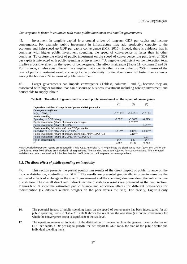
ECO/WKP(2016)68

27

Convergence is faster in countries with more public investment and smaller governments

45. Investment in tangible capital is a crucial driver of long-run GDP per capita and income

convergence. For example, public investment in infrastructure may add productive capacity to the

economy and help speed up GDP per capita convergence (IMF, 2015). Indeed, there is evidence that in

countries with higher public investment spending, the speed of convergence is faster than in other

countries. To capture the effect of public investment on the speed of convergence, the past level of GDP

per capita is interacted with public spending on investment.16

A negative coefficient on the interaction term

implies a positive effect on the speed of convergence. The effect is sizeable (Table 11, columns 2 and 3).

For instance, all else equal, the estimate implies that a country that is among the top 25% in terms of the

level of public investment would converge to the productivity frontier about one-third faster than a country

among the bottom 25% in terms of public investment.

46. Larger governments can impede convergence (Table 8, columns 1 and 3), because they are

associated with higher taxation that can discourage business investment including foreign investment and

households to supply labour.

Table 8. The effect of government size and public investment on the speed of convergence

(1) (2) (3)

Dependent variable: Change in ln of potential GDP per capita

Conergence coefficient

ln(Yit−1/POPit−1) -0.015*** -0.015*** -0.013**

Public spending Spending to GDP ratioit-1 -0.022* -0.0030 -0.025* Public investment (share of primary spending) it-1 0.072*** Public investment (share of GDP) it-1 0.21***

Public spending interacted with past GDP per capita Spending to GDP ratioit-1*ln(Y it-1/POP it-1) 0.11*** 0.028 0.096*** Public investment (share of primary spending) it-1*ln(Y it-1/POP it-1) -0.12*** Public investment (share of GDP) it-1*ln(Y it-1/POP it-1) -0.37**

No. of observations 547 547 547 R

2 0.757 0.783 0.783

Note: Detailed regression results are reported in Table A1.6. Asterisks (*, **, ***) indicate the significance level (10%, 5%, 1%) of the coefficients. Year fixed effects are included in all regressions. The standard errors are adjusted for country clusters. The interacted variables are mean centered, which implies that the coefficients can be interpreted as average effects.

5.3. The direct effect of public spending on inequality

47. This section presents the partial equilibrium results of the direct impact of public finance on the

income distribution, controlling for GDP.17

The results are presented graphically in order to visualise the

estimated effects of a change in the size of government and the spending structure along the entire income

distribution. The overall direct and indirect income distribution results are presented in the next section.

Figures 6 to 8 show the estimated public finance and education effects for different preferences for

redistribution (i.e. different relative weights on the poor versus the rich). For brevity, Figure 9 only

16. The potential impact of public spending items on the speed of convergence has been investigated for all

public spending items in Table 2. Table 8 shows the result for the one item (i.e. public investment) for

which the convergence effect is significant at the 5% level.

17. The equations regress an indicator of the distribution of income, such as the general mean or deciles on

GDP per capita, GDP per capita growth, the net export to GDP ratio, the size of the public sector and

individual spending items.

ECO/WKP(2016)68

28

presents the results for the spending items with a significant difference between the effect on the poor and

the effect on the rich.18

48. There is evidence that larger and more effective governments reduce inequality. Indeed, the

sensitivity of household disposable income to changes in the size of the government is positive and

significant at low incomes, while it is negative and significant at high incomes (Figure 6). Larger

governments can also be associated with a larger share of in-kind benefits; this increases the gap between

GDP (which includes in-kind benefits) and disposable income (which does not include in-kind benefits). In

addition, an increase in government effectiveness is beneficial for the poor, with no significant effect for

the rich (Figure 7).19

This finding may reflect that more effective governments are associated with better

targeting of disadvantaged groups and more cost-efficient delivery of transfer programmes.

Figure 6. Larger governments reduce inequality

Estimated direct impact of the size of the government along the income distribution

Note: The figure shows the effect along the income distribution of an increase of the size of the government by one GDP percentage point. For instance, a one percentage point increase of the size of the government increases the disposable income of the poor (α = -4) by 1.5%. The direct impact excludes any indirect impact of the change in policy on growth. Robustness checks with deciles instead of the general mean are reported in Figure A1.1.

18. The direct distributional effect of public spending on research and development is also not reported here

because the difference between the effect on the poor and the effect on the rich is not significant.

19. This finding is from a specification that includes both government size and government effectiveness. The

interaction between these two variables is not included because it is not significant along the income

distribution.

-2.0

-1.5

-1.0

-0.5

0.0

0.5

1.0

1.5

2.0

2.5

-4 -3 -2 -1 0 1 2 3 4 5 6

Estimated effect 90% confidence interval Effect on the mean disposable incomePer cent

General mean parameter α

The poor The lower-middle class Mean income The upper-middle class The rich

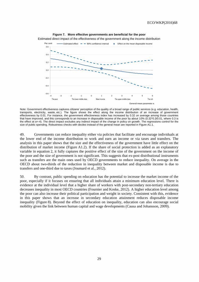
ECO/WKP(2016)68

29

Figure 7. More effective governments are beneficial for the poor

Estimated direct impact of the effectiveness of the government along the income distribution

Note: Government effectiveness captures citizens’ perception of the quality of a broad range of public services (e.g. education, health, transports, electricity, waste, etc.). The figure shows the effect along the income distribution of an increase of government effectiveness by 0.01. For instance, the government effectiveness index has increased by 0.32 on average among those countries that have improved, and this corresponds to an increase in disposable income of the poor by about 10% (0.32*0.3/0.01, where 0.3 is the effect at α=-4). The direct impact excludes any indirect impact of the change in policy on growth. The regressions control for the size of public spending. Robustness checks with deciles instead of the general mean are reported in Figure A1.1.

49. Governments can reduce inequality either via policies that facilitate and encourage individuals at

the lower end of the income distribution to work and earn an income or via taxes and transfers. The

analysis in this paper shows that the size and the effectiveness of the government have little effect on the

distribution of market income (Figure A1.2). If the share of social protection is added as an explanatory

variable in equation 2, it fully captures the positive effect of the size of the government on the income of

the poor and the size of government is not significant. This suggests that ex-post distributional instruments

such as transfers are the main ones used by OECD governments to reduce inequality. On average in the

OECD about two-thirds of the reduction in inequality between market and disposable income is due to

transfers and one-third due to taxes (Joumard et al., 2012).

50. By contrast, public spending on education has the potential to increase the market income of the

poor, especially if it focuses on ensuring that all individuals attain a minimum education level. There is

evidence at the individual level that a higher share of workers with post-secondary non-tertiary education

decreases inequality in most OECD countries (Fournier and Koske, 2012). A higher education level among

the poor can also increase their political participation and weight in society. Consistent with this, evidence

in this paper shows that an increase in secondary education attainment reduces disposable income

inequality (Figure 8). Beyond the effect of education on inequality, education can also encourage social

mobility given the link between human capital and wage developments (Causa and Johansson, 2009).

-0.6

-0.4

-0.2

0.0

0.2

0.4

0.6

-4 -3 -2 -1 0 1 2 3 4 5 6




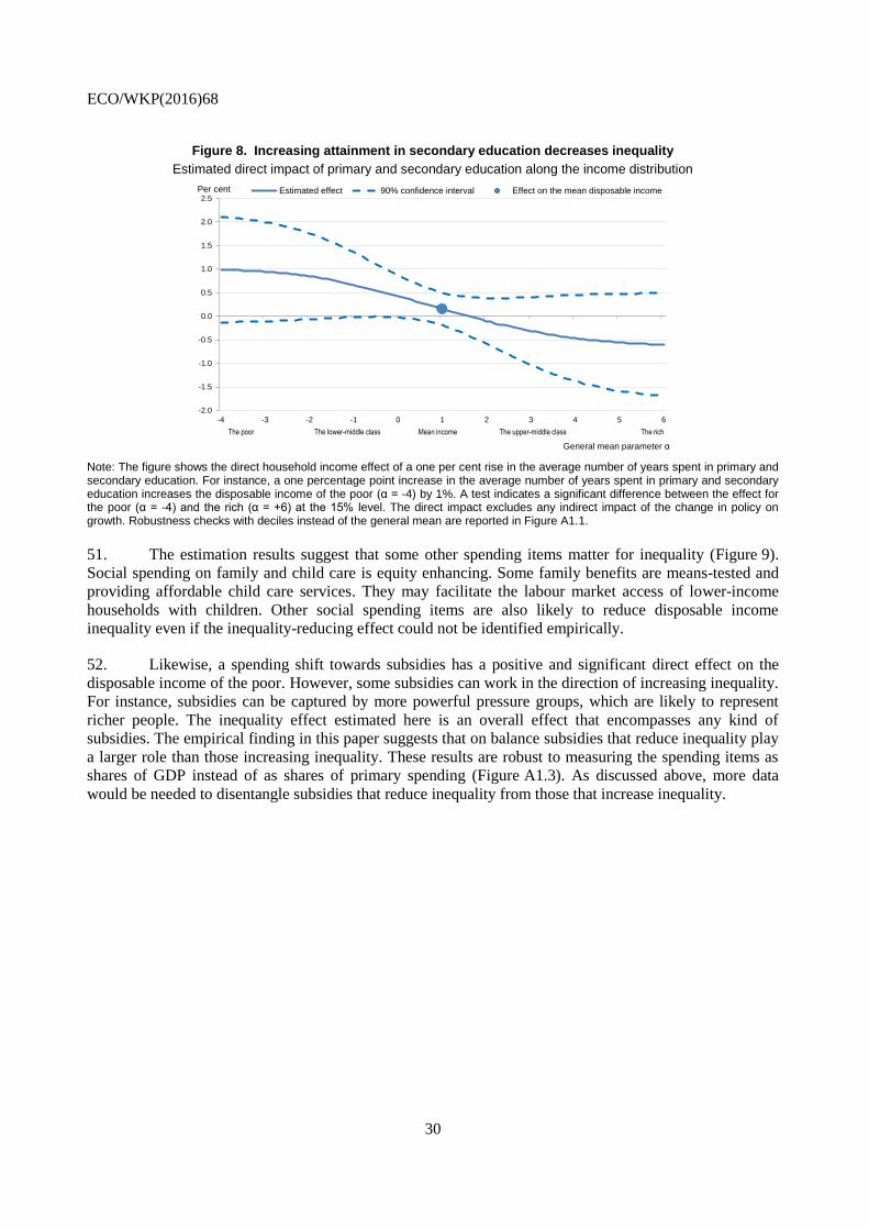
ECO/WKP(2016)68

30

Figure 8. Increasing attainment in secondary education decreases inequality

Estimated direct impact of primary and secondary education along the income distribution

Note: The figure shows the direct household income effect of a one per cent rise in the average number of years spent in primary and secondary education. For instance, a one percentage point increase in the average number of years spent in primary and secondary education increases the disposable income of the poor (α = -4) by 1%. A test indicates a significant difference between the effect for the poor (α = -4) and the rich (α = +6) at the 15% level. The direct impact excludes any indirect impact of the change in policy on growth. Robustness checks with deciles instead of the general mean are reported in Figure A1.1.

51. The estimation results suggest that some other spending items matter for inequality (Figure 9).

Social spending on family and child care is equity enhancing. Some family benefits are means-tested and

providing affordable child care services. They may facilitate the labour market access of lower-income

households with children. Other social spending items are also likely to reduce disposable income

inequality even if the inequality-reducing effect could not be identified empirically.

52. Likewise, a spending shift towards subsidies has a positive and significant direct effect on the

disposable income of the poor. However, some subsidies can work in the direction of increasing inequality.

For instance, subsidies can be captured by more powerful pressure groups, which are likely to represent

richer people. The inequality effect estimated here is an overall effect that encompasses any kind of

subsidies. The empirical finding in this paper suggests that on balance subsidies that reduce inequality play

a larger role than those increasing inequality. These results are robust to measuring the spending items as

shares of GDP instead of as shares of primary spending (Figure A1.3). As discussed above, more data

would be needed to disentangle subsidies that reduce inequality from those that increase inequality.

-2.0

-1.5

-1.0

-0.5

0.0

0.5

1.0

1.5

2.0

2.5

-4 -3 -2 -1 0 1 2 3 4 5 6




ECO/WKP(2016)68

31

Figure 9. Some spending items matter for inequality

Estimated direct impact of spending items along the income distribution

A: Subsidies B: Family benefits

Note: Panel A and B show the direct effect along the income distribution of a one percentage point increase of the share of subsidies or family benefits in primary spending. For instance, Panel A shows that a one percentage point increase in the share of subsidies in primary spending increases the disposable income of the poor (α = -4) by 5%. A test indicates a significant difference between the effect for the poor (α = -4) and the rich (α = +6) at the 5% level for family benefits and at the 1% level for subsidies. The direct impact excludes any indirect impact of the change in policy on growth. Robustness checks with deciles instead of the general mean are reported in Figure A1.3.

53. There is no evidence in the data that the spending share of other items than subsidies and family

benefits in Table 2 have a different effect on the lower-end than on the higher-end of the income

distribution. This means that the redistributive effects are relatively small, or may be too heterogeneous

across countries, so that it is not possible to identify a general pattern. For instance, a rise of pension

spending has no visible effect on inequality. However, if the average income of pensioners is below the

country average, increasing pension spending can decrease inequality, while if the average income of

pensioners is above the country average, increasing pension spending increases inequality. The inequality

effect of an increase in pension spending also depends on whether it is targeted or not.

6. Simulations of growth and inequality effects of public spending reforms

6.1. Illustrative growth gains

54. To gauge the economic magnitude of the estimates, simulations illustrate the potential impact of

a change in the size and the structure of public spending on long-term growth. Two types of simulations

are run. In the case of spending on investment, pensions and subsidies, the simulations consider the impact

of a change in the amount of spending on the long-run level of GDP. The end of the time horizon in these

simulations is 2060.20

Education spending takes time to translate into effects on educational attainment of

the population. Reflecting this, the education simulation illustrates the impact of a change in the stock of

the adjusted average years of schooling on the long-run level of GDP. This simulation does not necessarily

reflect a rise in education spending, it could also reflect education policy reforms.

55. The simulations are specified in the following way: (i) in countries where the mean PISA score or

average years of schooling are below the average level of countries in the top half of the sample,

educational attainments will gradually converge to this level, where the reform is phased in over 45 years;

(ii) in countries where public investment to potential GDP is below the average ratio of countries in the top

half of the sample, public investment will converge to this average ratio; and (iii) in countries where

spending to the potential GDP ratio on subsidies and pensions are above the average level of countries in

20. As the convergence coefficient is 2% it takes a very long time to reach the long-term effect. The effect

after 45 years of a reform that is phased in instantaneously represents roughly two thirds of the long-term

effect.

-8

-6

-4

-2

0

2

4

6

8

10

-4 -3 -2 -1 0 1 2 3 4 5 6




-6

-4

-2

0

2

4

6

8

10

12

14

-4 -3 -2 -1 0 1 2 3 4 5 6




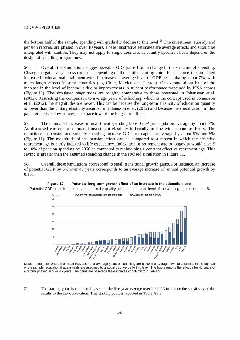
ECO/WKP(2016)68

32

the bottom half of the sample, spending will gradually decline to this level.21

The investment, subsidy and

pension reforms are phased in over 10 years. These illustrative estimates are average effects and should be

interpreted with caution. They may not apply to single countries as country-specific effects depend on the

design of spending programmes.

56. Overall, the simulations suggest sizeable GDP gains from a change in the structure of spending.

Cleary, the gains vary across countries depending on their initial starting point. For instance, the simulated

increase in educational attainment would increase the average level of GDP per capita by about 7%, with

much larger effects in some countries (e.g. Chile, Mexico and Turkey). On average about half of the

increase in the level of income is due to improvements in student performance measured by PISA scores

(Figure 10). The simulated magnitudes are roughly comparable to those presented in Johansson et al.

(2012). Restricting the comparison to average years of schooling, which is the concept used in Johansson

et al. (2012), the magnitudes are lower. This can be because the long-term elasticity of education quantity

is lower than the unitary elasticity assumed in Johansson et al. (2012) and because the specification in this

paper embeds a slow convergence pace toward the long-term effect.

57. The simulated increases in investment spending boost GDP per capita on average by about 7%.

As discussed earlier, the estimated investment elasticity is broadly in line with economic theory. The

reductions in pension and subsidy spending increase GDP per capita on average by about 9% and 5%

(Figure 11). The magnitude of the pension effect can be compared to a reform in which the effective

retirement age is partly indexed to life expectancy. Indexation of retirement age to longevity would save 5

to 10% of pension spending by 2060 as compared to maintaining a constant effective retirement age. This

saving is greater than the assumed spending change in the stylised simulation in Figure 11.

58. Overall, these simulations correspond to small transitional growth gains. For instance, an increase

of potential GDP by 5% over 45 years corresponds to an average increase of annual potential growth by

0.1%.

Figure 10. Potential long-term growth effect of an increase in the education level

Potential GDP gains from improvements in the quality adjusted education level of the working-age population, %

Note: In countries where the mean PISA score or average years of schooling are below the average level of countries in the top half of the sample, educational attainments are assumed to gradually converge to this level. The figure reports the effect after 45 years of a reform phased in over 45 years. The gains are based on the estimates of column 2 in Table 5.

21. The starting point is calculated based on the five-year average over 2009-13 to reduce the sensitivity of the

results to the last observation. This starting point is reported in Table A1.2.

0

5

10

15

20

25

30

Quantity of education (years of schooling) Quality of education (PISA)Per cent

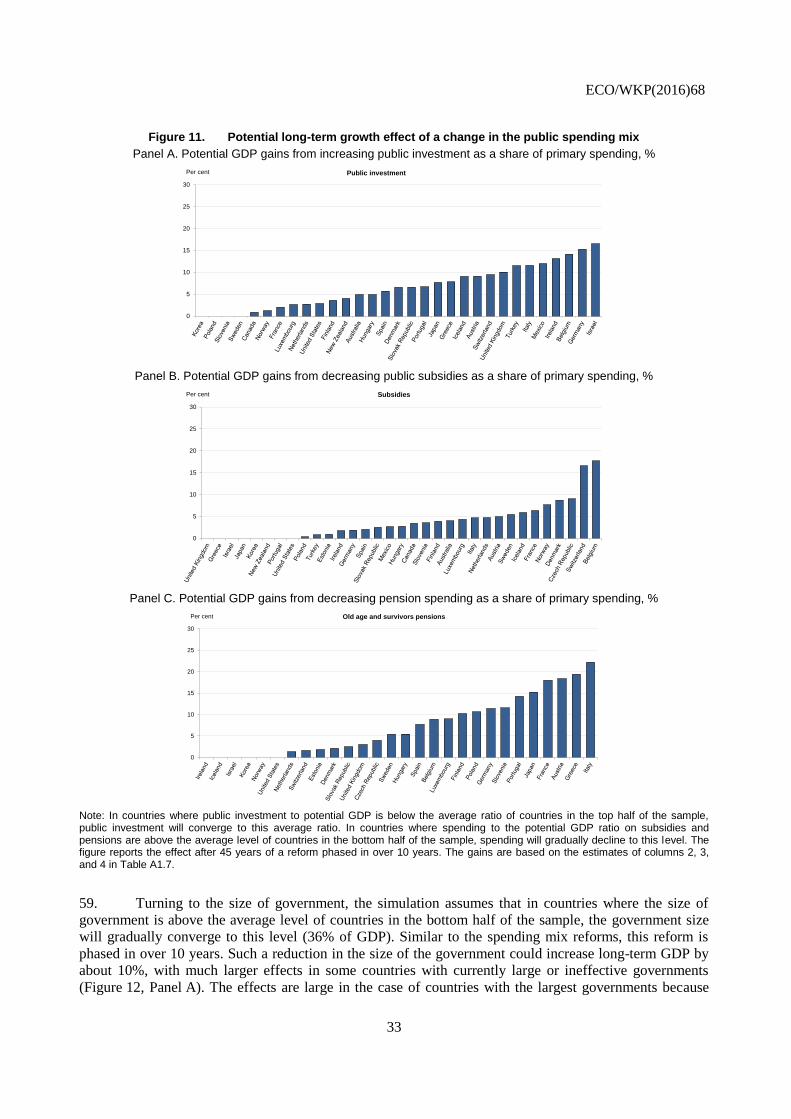
ECO/WKP(2016)68

33

Figure 11. Potential long-term growth effect of a change in the public spending mix

Panel A. Potential GDP gains from increasing public investment as a share of primary spending, %

Panel B. Potential GDP gains from decreasing public subsidies as a share of primary spending, %

Panel C. Potential GDP gains from decreasing pension spending as a share of primary spending, %

Note: In countries where public investment to potential GDP is below the average ratio of countries in the top half of the sample, public investment will converge to this average ratio. In countries where spending to the potential GDP ratio on subsidies and pensions are above the average level of countries in the bottom half of the sample, spending will gradually decline to this level. The figure reports the effect after 45 years of a reform phased in over 10 years. The gains are based on the estimates of columns 2, 3, and 4 in Table A1.7.

59. Turning to the size of government, the simulation assumes that in countries where the size of

government is above the average level of countries in the bottom half of the sample, the government size

will gradually converge to this level (36% of GDP). Similar to the spending mix reforms, this reform is

phased in over 10 years. Such a reduction in the size of the government could increase long-term GDP by

about 10%, with much larger effects in some countries with currently large or ineffective governments

(Figure 12, Panel A). The effects are large in the case of countries with the largest governments because

0

5

10

15

20

25

30

Public investmentPer cent

0

5

10

15

20

25

30

Subsidies Per cent

0

5

10

15

20

25

30

Old age and survivors pensionsPer cent

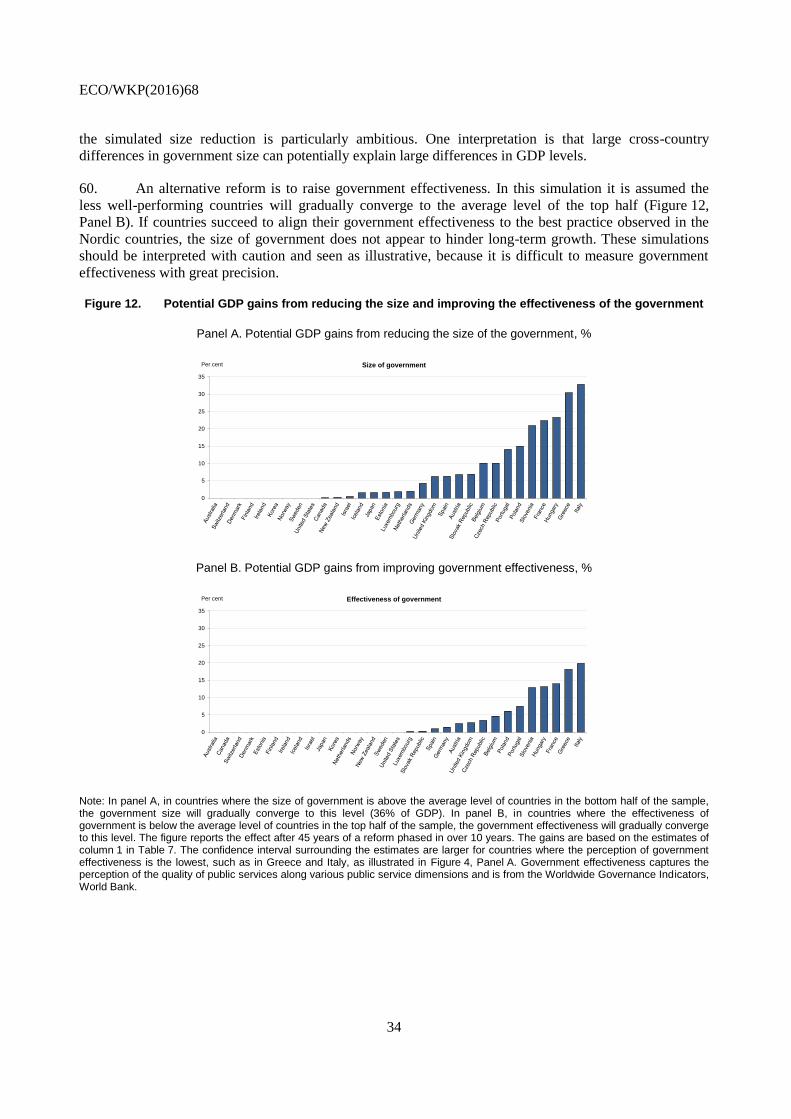
ECO/WKP(2016)68

34

the simulated size reduction is particularly ambitious. One interpretation is that large cross-country

differences in government size can potentially explain large differences in GDP levels.

60. An alternative reform is to raise government effectiveness. In this simulation it is assumed the

less well-performing countries will gradually converge to the average level of the top half (Figure 12,

Panel B). If countries succeed to align their government effectiveness to the best practice observed in the

Nordic countries, the size of government does not appear to hinder long-term growth. These simulations

should be interpreted with caution and seen as illustrative, because it is difficult to measure government

effectiveness with great precision.

Figure 12. Potential GDP gains from reducing the size and improving the effectiveness of the government

Panel A. Potential GDP gains from reducing the size of the government, %

Panel B. Potential GDP gains from improving government effectiveness, %

Note: In panel A, in countries where the size of government is above the average level of countries in the bottom half of the sample, the government size will gradually converge to this level (36% of GDP). In panel B, in countries where the effectiveness of government is below the average level of countries in the top half of the sample, the government effectiveness will gradually converge to this level. The figure reports the effect after 45 years of a reform phased in over 10 years. The gains are based on the estimates of column 1 in Table 7. The confidence interval surrounding the estimates are larger for countries where the perception of government effectiveness is the lowest, such as in Greece and Italy, as illustrated in Figure 4, Panel A. Government effectiveness captures the perception of the quality of public services along various public service dimensions and is from the Worldwide Governance Indicators, World Bank.

0

5

10

15

20

25

30

35

Size of governmentPer cent

0

5

10

15

20

25

30

35

Effectiveness of governmentPer cent

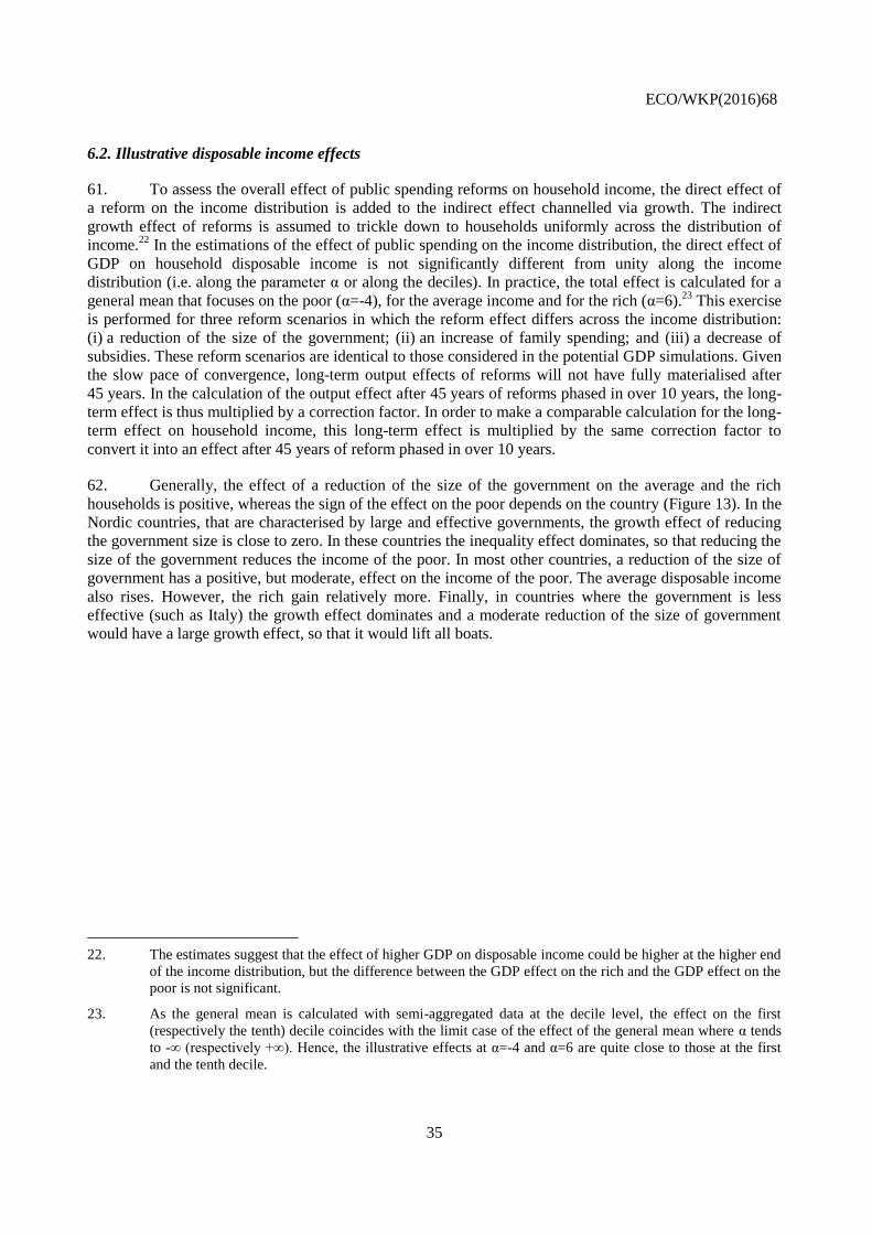
ECO/WKP(2016)68

35

6.2. Illustrative disposable income effects

61. To assess the overall effect of public spending reforms on household income, the direct effect of

a reform on the income distribution is added to the indirect effect channelled via growth. The indirect

growth effect of reforms is assumed to trickle down to households uniformly across the distribution of

income.22

In the estimations of the effect of public spending on the income distribution, the direct effect of

GDP on household disposable income is not significantly different from unity along the income

distribution (i.e. along the parameter α or along the deciles). In practice, the total effect is calculated for a

general mean that focuses on the poor (α=-4), for the average income and for the rich (α=6).23

This exercise

is performed for three reform scenarios in which the reform effect differs across the income distribution:

(i) a reduction of the size of the government; (ii) an increase of family spending; and (iii) a decrease of

subsidies. These reform scenarios are identical to those considered in the potential GDP simulations. Given

the slow pace of convergence, long-term output effects of reforms will not have fully materialised after

45 years. In the calculation of the output effect after 45 years of reforms phased in over 10 years, the long-

term effect is thus multiplied by a correction factor. In order to make a comparable calculation for the long-

term effect on household income, this long-term effect is multiplied by the same correction factor to

convert it into an effect after 45 years of reform phased in over 10 years.

62. Generally, the effect of a reduction of the size of the government on the average and the rich

households is positive, whereas the sign of the effect on the poor depends on the country (Figure 13). In the

Nordic countries, that are characterised by large and effective governments, the growth effect of reducing

the government size is close to zero. In these countries the inequality effect dominates, so that reducing the

size of the government reduces the income of the poor. In most other countries, a reduction of the size of

government has a positive, but moderate, effect on the income of the poor. The average disposable income

also rises. However, the rich gain relatively more. Finally, in countries where the government is less

effective (such as Italy) the growth effect dominates and a moderate reduction of the size of government

would have a large growth effect, so that it would lift all boats.

22. The estimates suggest that the effect of higher GDP on disposable income could be higher at the higher end

of the income distribution, but the difference between the GDP effect on the rich and the GDP effect on the

poor is not significant.

23. As the general mean is calculated with semi-aggregated data at the decile level, the effect on the first

(respectively the tenth) decile coincides with the limit case of the effect of the general mean where α tends

to -∞ (respectively +∞). Hence, the illustrative effects at α=-4 and α=6 are quite close to those at the first

and the tenth decile.

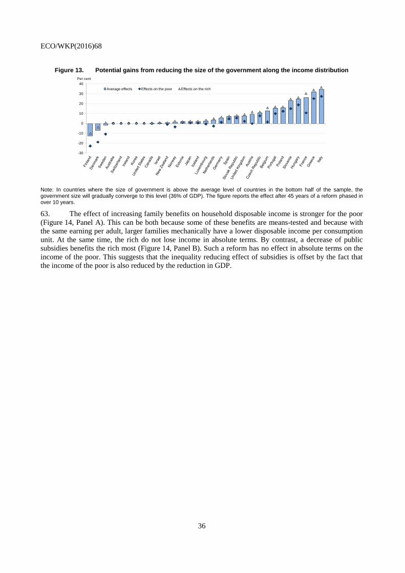
ECO/WKP(2016)68

36

Figure 13. Potential gains from reducing the size of the government along the income distribution

Note: In countries where the size of government is above the average level of countries in the bottom half of the sample, the government size will gradually converge to this level (36% of GDP). The figure reports the effect after 45 years of a reform phased in over 10 years.

63. The effect of increasing family benefits on household disposable income is stronger for the poor

(Figure 14, Panel A). This can be both because some of these benefits are means-tested and because with

the same earning per adult, larger families mechanically have a lower disposable income per consumption

unit. At the same time, the rich do not lose income in absolute terms. By contrast, a decrease of public

subsidies benefits the rich most (Figure 14, Panel B). Such a reform has no effect in absolute terms on the

income of the poor. This suggests that the inequality reducing effect of subsidies is offset by the fact that

the income of the poor is also reduced by the reduction in GDP.

-30

-20

-10

0

10

20

30

40

Average effects Effects on the poor Effects on the rich

Per cent

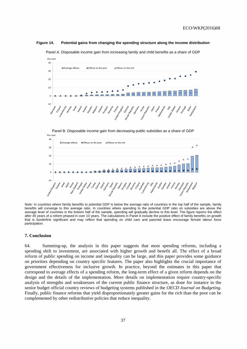
ECO/WKP(2016)68

37

Figure 14. Potential gains from changing the spending structure along the income distribution

Panel A. Disposable income gain from increasing family and child benefits as a share of GDP

Panel B. Disposable income gain from decreasing public subsidies as a share of GDP

Note: In countries where family benefits to potential GDP is below the average ratio of countries in the top half of the sample, family benefits will converge to this average ratio. In countries where spending to the potential GDP ratio on subsidies are above the average level of countries in the bottom half of the sample, spending will gradually decline to this level. The figure reports the effect after 45 years of a reform phased in over 10 years. The calculations in Panel A include the positive effect of family benefits on growth that is borderline significant and may reflect that spending on child care and parental leave encourage female labour force participation.

7. Conclusion

64. Summing-up, the analysis in this paper suggests that most spending reforms, including a

spending shift to investment, are associated with higher growth and benefit all. The effect of a broad

reform of public spending on income and inequality can be large, and this paper provides some guidance

on priorities depending on country specific features. The paper also highlights the crucial importance of

government effectiveness for inclusive growth. In practice, beyond the estimates in this paper that

correspond to average effects of a spending reform, the long-term effect of a given reform depends on the

design and the details of the implementation. More details on implementation require country-specific

analysis of strengths and weaknesses of the current public finance structure, as done for instance in the

senior budget official country reviews of budgeting systems published in the OECD Journal on Budgeting.

Finally, public finance reforms that yield disproportionately greater gains for the rich than the poor can be

complemented by other redistributive policies that reduce inequality.

-10

0

10

20

30

40


Per cent

-10

0

10

20

30

40


Per cent

ECO/WKP(2016)68

38

REFERENCES

Afonso, A. and J. Tovar-Valles (2011), “Economic Performance and Government Size”, Working Paper

Series, No. 1399, European Central Bank.

Alesina, A., R. Baqir and W. Easterly (2000), “Redistributive Public Employment”, Journal of Urban

Economics, Vol. 48, pp. 219-241.

Algan Y. and P. Cahuc (2014), “Trust, Well-Being and Growth: New Evidence and Policy Implications”,

in Aghion, P. and S. N. Durlauf, eds., Handbook of Economic Growth, Elsevier Science, pp.49-120.

Andrews, D. and C. Criscuolo (2013), “Knowledge-Based Capital, Innovation and Resource Allocation”,

OECD Economics Department Working Papers, No. 1046, OECD Publishing, Paris.

Arellano, M. A. and S. Bond (1991), “Some Tests of Specification for Panel Data: Monte Carlo Evidence

and an Application to Employment Equations”, Review of Economic Studies, Vol. 58(2), pp. 277-97.

Arellano, M. and O. Bover (1995), “Another Look at the Instrumental Variable Estimation of Error-

Components Models”, Journal of Econometrics, Vol. 68.

Armey, D. (1995), The Freedom Revolution, Washington: Regnery Publishing.

Arnold, J. et al. (2011a), “Tax Policy for Economic Recovery and Growth”, Economic Journal, Vol. 121,

pp. F59-F80.

Arnold, J., A. Bassanini and S. Scarpetta (2011b), “Solow or Lucas? Testing Speed of Convergence on a

Panel of OECD Countries”, Research in Economics, Vol. 65, pp. 110-123.

Barro, R. J. (1990), “Government Spending in a Simple Model of Endogenous Growth”, Journal of

Political Economy, 98 (5).

Barro, R. J. (2015), “Convergence and Modernisation”, The Economic Journal, Vol. 125, pp. 911-942.

Becker, G. S. (1985), “Public Policies, Pressure Groups, and Dead Weight Costs”, Journal of Public

Economics, Vol. 28, pp. 329-347.

Bergh, A. and M. Henrekson (2011), “Government Size and Growth: A Survey and Interpretation of the

Evidence", IFN Working Paper, No. 858.

Bloch D., J.M. Fournier, D. Gonzales and A. Pina (2016), “Trends in Public Finances: Insights from a New

Detailed Dataset”, OECD Economic Department Working Papers, No. 1345, OECD Publishing,

Paris.

ECO/WKP(2016)68

39

Blöchliger, H., B. Égert and K. Bonesmo Fredriksen (2013), “Fiscal Federalism and its Impact on

Economic Activity, Public Investment and the Performance of Educational Systems”, OECD

Economics Department Working Papers, No. 1051, OECD Publishing, Paris.

Blundell, R. and S. Bond (2000), “GMM Estimation with Persistent Panel Data: An Application to

Production Functions”, Econometric Reviews, Vol. 19.

Causa, O. et al. (2014a), “Economic Growth from the Household Perspective: GDP and Income

Distribution Developments across OECD Countries”, OECD Economics Department Working

Papers, No. 1111, OECD Publishing, Paris.

Causa, O., A. de Serres and N. Ruiz (2014b), “Can Pro-growth Policies Lift All Boats? An Analysis Based

on Household Disposable Income”, OECD Economics Department Working Papers, No. 1180,

OECD Publishing, Paris.

Causa, O. and Å. Johansson (2009), “Intergenerational Social Mobility”, OECD Economics Department

Working Papers, No. 707, OECD Publishing, Paris.

Chen, S. and C. Lee (2005), “Government Size and Economic Growth in Taiwan: a Threshold Regression

Approach”, Journal of Policy Modelling, 27, pp. 1051-1066.

Coleman, J. S. (1966), “Equality of Educational Opportunity”, Ann Arbor, MI: Inter-university

Consortium for Political and Social Research.

Cournède, B., A. Goujard and A. Pina (2013), “How to Achieve Growth- and Equity-friendly Fiscal

Consolidation?: A Proposed Methodology for Instrument Choice with an Illustrative Application to

OECD Countries”, OECD Economics Department Working Papers, No. 1088, OECD Publishing,

Paris.

Cournède, B. and O. Denk (2015), “Finance and Economic Growth in OECD and G20 Countries”, OECD

Economics Department Working Papers, No. 1223, OECD Publishing, Paris.

Easterly, W. and S. Rebelo (1993), “Fiscal Policy and Economic Growth: An Empirical Investigation”,

Journal of Monetary Economics, Elsevier, Vol. 32, No. 3, pp. 417-458.

Fall, F. and J.M. Fournier (2015), "Macroeconomic Uncertainties, Prudent Debt Targets and Fiscal Rules",


Förster, M. and I. G. Tóth (2015), “Cross-Country Evidence of the Multiple Causes of Inequality Changes

in the OECD Area”, in: A. B. Atkinson and F. Bourguignon (eds.), Handbook of Income

Distribution, Volume 2B, Chapter 19. Elsevier, North Holland B.v.

Fournier, J.M. (2016), “The Positive Effect of Public Investment on Potential Growth”, OECD Economics

Department Working Paper, No. 1347, OECD Publishing, Paris.

Fournier, J.M. and I. Koske (2012), "Less Income Inequality and More Growth – Are They Compatible?

Part 7. The Drivers of Labour Earnings Inequality – An Analysis Based on Conditional and

Unconditional Quantile Regressions”, OECD Economics Department Working Papers, No. 930,

OECD Publishing, Paris.

Freeman, R. (1995), “The Large Welfare State as a System”, American Economic Review, 85 (2), 16-21.

ECO/WKP(2016)68

40

Gemmell, N., R. Kneller and I. Sanz (2014), “Does the Composition of Government Expenditure Matter

for Long-run GDP Levels?”, Working Paper, No. 10/2014, Victoria University.

Hanushek, E. A. and L. Woessmann (2011), “The Economics of International Differences in Educational

Achievement”, in: Hanushek, E. A., S. Machin and L. Woessmann (eds.), Handbook of the

Economics of Education, Vol. 3 (pp. 89–200). Amsterdam: North Holland.

Hanushek, E. and L. Woessmann (2012), “Do Better Schools Lead to More Growth? Cognitive Skills,

Economic Outcomes, and Causation”, Journal of Economic Growth, Vol. 17.

Hermansen, M., N. Ruiz and O. Causa (2016), “The Distribution of the Growth Dividends”, OECD

Economics Department Working Paper, No. 1343, OECD Publishing, Paris.

Hurwicz, L. (1950), “Least Squares Bias in Time Series”, in: T.C. Koopmans (ed.), Statistical Inference in

Dynamic Economic Models, Wiley, New York.

IMF (2015), “Making Public Investment more Efficient”, IMF.

Johansson, A. (2016), "Public Finance, Economic Growth and Inequality: A Survey of the Evidence",

OECD Economic Department Working Papers, No. 1346, OECD Publishing, Paris.

Johansson Å, Y. Guillemette, F. Murtin, D. Turner, G. Nicoletti, C. de la Maisonneuve, P. Bagnoli, G.

Bousquet and F. Spinelli (2012), “Long-term Growth Scenarios”, OECD Economics Department

Working Papers, No. 1000, OECD Publishing, Paris.

Joumard, I., M. Pisu and D. Bloch (2012), “Less Income Inequality and More Growth – Are They

Compatible? Part 3. Income Redistribution via Taxes and Transfers Across OECD Countries”,


Kneller, R., M. Bleaney and N. Gemmell (1999), “Fiscal Policy and Growth: Evidence from OECD

Countries”, Journal of Public Economics, Elsevier, Vol. 74(2).

Koeniger, W., M. Leonardi and L. Nunziata (2007), “Labor Market Institutions and Wage Inequality”,

Industrial and Labor Relations Review, Vol. 60, No. 3, pp. 340-356.

Krueger, A., B. and M. Lindahl (2001) “Education for Growth: Why and For Whom?”, Journal of

Economic Literature, Vol. 39, pp. 1101-1136.

Lucas, R. (1988), “On the Mechanics of Economic Development”, Journal of Monetary Economics,

Vol. 22.

Mankiw, G.N., D. Romer and D. N. Weil (1992), “A Contribution to the Empirics of Economic Growth”,

Quarterly Journal of Economics, Vol. 107, pp. 407–437.

Myles, G. (2009), “Economic Growth and the Role of Taxation”, OECD Economics Department Working

Papers, No. 713-715, OECD Publishing, Paris.

Nickell, S. (1981), “Biases in Dynamic Models with Fixed Effects”, Econometrica, Econometric Society,

Vol. 49(6), pp. 1417-26.

ECO/WKP(2016)68

41

Nerlove, M. (2000), “Growth Rate Convergence, Fact or Artefact? An Essay on Panel Data Econometrics”,

Chapter 6 in: Krishnakumar, J. and E. Ronchetti, eds., Panel Data Econometrics: Future Directions,

pp. 3-33.

OECD (2001), Competition Policy in Subsidies and State Aid, OECD Publishing, Paris.

OECD (2013), Trust in Government: Assessing the Evidence, Understanding the Policies, OECD

Publishing, Paris.

OECD (2014), “PISA 2012 Results: What Students Know and Can Do, Student Performance in

Mathematics, Reading and Science”, Vol. I, revised edition, OECD Publishing, Paris.

Orphanides, A. and S. van Norden (2002), “The Unreliability of Output-Gap Estimates in Real Time”, The

Review of Economics and Statistics, Vol. 84, No. 4, pp. 569-583.

Pevcin, P. (2004), “Does Optimal Spending Size of Government Exist?”, Paper presented at the European

Group of Public Administration Conference, 1-4 September 2004, Ljubljana, Slovenia.

Price, R. W., T. Dang and J. Botev (2015), "Adjusting Fiscal Balances for the Business Cycle: New Tax

and Expenditure Elasticity Estimates for OECD Countries", OECD Economics Department Working

Papers, No. 1275, OECD Publishing, Paris.

Romer, P. (1990), “Human Capital and Growth: Theory and Evidence”, Carnegie Rochester Conference

Series on Public Policy, Vol. 32.

Roodman, D. (2009), “A Note on the Theme of Too Many Instruments”, Oxford Bulletin of Economics and

Statistics, Vol. 71, pp. 135-158.

Salverda, W. and D. Checchi (2014), "Labour-Market Institutions and the Dispersion of Wage Earnings",

IZA Discussion Paper, No. 8220.

Slemrod, J. (1995), “What Do Cross-Country Studies Teach about Government Involvement, Prosperity

and Economic Growth?”, Brookings Papers on Economic Activity, pp. 373-431.

Solow, R. (1956), “A Contribution to the Theory of Economic Growth”, The Quarterly Journal of

Economics, Vol. 70, No. 1.

Teles, V.K. and C.C. Mussolini (2014), “Public Debt and the Limits of Fiscal Policy to Increase Economic

Growth”, European Economic Review, Vol. 66.

Uzawa, H. (1965), “Optimum Technical Change in an Aggregative Model of Economic Growth”,

International Economic Review, Vol. 6, pp. 18-31.

Vedder, R. and L. Gallaway (1998), “Government Size and Economic Growth”, Paper prepared for the

Joint Economic Committee, Washington, D.C.

ECO/WKP(2016)68

42

ANNEX 1

Public spending breakdown and data definitions

Table A1.1. Public spending breakdown

Note: The mapping of National Accounts Classification of the Functions of Government (COFOG) data into the 11 spending items used in this paper is highlighted by the numbers in the table. For instance, education (item 1) consists of social benefits and in kind transfers, wages and intermediate consumption in education. The columns in the table refer to national accounts transactions (codes in parentheses refer to Annual National Accounts Table 11 COFOG codes or Economic Outlook database variable codes), while rows show the breakdown by functions in the COFOG classification (the codes in parentheses refer to COFOG function codes). The areas coloured in pink refer to data extracted from Annual National Accounts Table 11 (COFOG), the areas in blue refer to data taken from the Economic Outlook database, and the areas without shading are calculated as a difference between total expenditure (YPGT) from the Economic Outlook database and the other aforementioned items.

Social benefits

and transfers

in kind

(D62_D631XX)

Wages

(D1)

Intermediate

consumption

(P2)

Subsidies

(TSUB)

Investment

(IGAA)

Interest

payments

(YPEPG)

Inventory

changes

Capital

transfers

Other

primary

expen-

ditures

1 1 1 8 9 11 10 10 10

2 2 2 8 9 11 10 10 10

Sickness and disability (1001) 5 5 5 8 9 11 10 10 10

Family and children (1004) 7 7 7 8 9 11 10 10 10

Old age and survivors (1002 + 1003) 4 3 3 8 9 11 10 10 10

Unemployment (1005) 6 3 3 8 9 11 10 10 10

Other social protection (1006-09) 10 3 3 8 9 11 10 10 10

10 3 3 8 9 11 10 10 10

10 3 3 8 9 11 10 10 10

10 3 3 8 9 11 10 10 10

10 3 3 8 9 11 10 10 10

10 3 3 8 9 11 10 10 10

10 3 3 8 9 11 10 10 10

10 3 3 8 9 11 10 10 10

Economic affairs (040)

Environment protection (050)

Housing and community amenities (060)

Recreation, culture and religion (080)

Social

protection

(100)

Public order and safety (030)

Defence (020)

General public services (010)

Education (090)

Health (070)

Function

Transaction

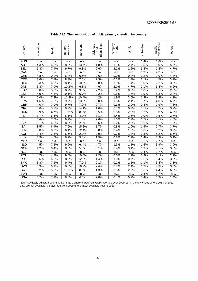
ECO/WKP(2016)68

43

Table A1.2. The composition of public primary spending by country

co

untr

y

ed

uca

tion

he

alth

ge

ne

ral

se

rvic

es

pe

nsio

ns

sic

kn

ess

an

d

dis

ab

ilities

un

em

plo

y

me

nt

fam

ily

su

bsid

ies

pu

blic

investm

en

t

oth

ers

AUS n.a. n.a. n.a. n.a. n.a. n.a. n.a. 1.4% 3.6% n.a.

AUT 4.3% 6.5% 8.9% 13.7% 1.8% 1.1% 2.4% 1.5% 3.0% 5.0%

BEL 5.8% 7.4% 9.7% 9.8% 2.6% 2.2% 2.2% 3.4% 2.4% 4.7%

CAN n.a. n.a. n.a. n.a. n.a. n.a. n.a. 1.3% 4.2% n.a.

CHE 4.8% 0.2% 6.4% 6.6% 2.6% 0.9% 0.4% 3.2% 3.0% 4.3%

CZE 3.6% 7.1% 8.3% 7.6% 2.3% 0.3% 1.3% 2.1% 4.5% 3.7%

DEU 3.3% 6.6% 8.1% 10.8% 2.8% 1.9% 1.4% 1.0% 2.2% 3.8%

DNK 5.8% 7.9% 10.2% 6.8% 4.6% 2.0% 4.7% 2.1% 3.4% 6.2%

ESP 3.8% 5.8% 8.7% 9.3% 2.2% 2.2% 0.6% 1.0% 3.5% 2.8%

EST 4.9% 4.4% 9.1% 6.7% 2.2% 0.5% 1.6% 0.9% 5.3% 2.4%

FIN 5.0% 7.2% 11.3% 10.4% 4.2% 1.9% 3.0% 1.3% 3.8% 4.1%

FRA 4.6% 7.2% 9.7% 13.5% 2.0% 1.5% 2.1% 1.7% 4.0% 6.7%

GBR 4.0% 7.0% 9.7% 7.2% 2.7% 0.3% 2.0% 0.4% 2.9% 7.3%

GRC 3.6% 5.7% 9.9% 14.1% 1.6% 0.7% 0.7% 0.5% 3.2% 3.9%

HUN 3.9% 4.7% 10.6% 8.3% 3.5% 0.5% 2.2% 1.2% 3.6% 4.8%

IRL 3.7% 6.5% 6.1% 4.9% 3.1% 2.4% 2.6% 1.0% 2.5% 3.7%

ISL 6.4% 7.0% 9.2% 1.8% 2.6% 1.0% 2.2% 1.7% 3.1% 4.0%

ISR 5.1% 4.8% 8.8% 2.9% 3.6% 0.2% 2.6% 0.6% 2.1% 7.0%

ITA 3.5% 6.4% 7.6% 15.2% 1.7% 0.8% 1.0% 1.5% 2.7% 3.7%

JPN 3.0% 6.7% 6.4% 12.4% 0.8% 0.4% 1.3% 0.6% 3.2% 3.9%

KOR 3.4% 3.5% 6.5% 2.0% 0.9% 0.3% 1.4% 0.3% 5.2% 6.6%

LUX 3.9% 4.5% 6.9% 9.8% 1.9% 0.8% 2.9% 1.4% 3.9% 5.1%

MEX n.a. n.a. n.a. n.a. n.a. n.a. n.a. 1.1% 2.7% n.a.

NLD 4.5% 7.5% 9.9% 6.4% 4.7% 1.3% 1.1% 1.5% 3.9% 3.9%

NOR 4.2% 6.4% 8.0% 5.6% 6.1% 0.4% 3.1% 1.9% 4.1% 3.0%

NZL n.a. n.a. n.a. n.a. n.a. n.a. n.a. 0.4% 3.7% n.a.

POL 4.7% 4.3% 9.0% 10.5% 2.2% 0.5% 1.2% 0.8% 5.1% 2.9%

PRT 5.6% 6.5% 8.6% 12.0% 1.4% 1.0% 0.7% 0.6% 3.4% 3.3%

SVK 3.8% 7.2% 9.4% 7.0% 2.1% 0.2% 1.5% 1.1% 3.4% 3.8%

SVN 5.3% 6.1% 8.6% 10.9% 2.4% 0.7% 2.1% 1.3% 4.3% 3.5%

SWE 5.2% 5.6% 10.2% 8.3% 4.3% 0.5% 2.3% 1.6% 4.4% 6.8%

TUR n.a. n.a. n.a. n.a. n.a. n.a. n.a. 0.8% 2.7% n.a.

USA 5.7% 7.9% 8.8% 4.6% 2.0% 0.4% 0.9% 0.4% 3.9% 1.4%

Note: Cyclically adjusted spending items as a share of potential GDP, average over 2009-13. In the few cases where 2013 or 2012 data are not available, the average from 2009 to the latest available year is used.

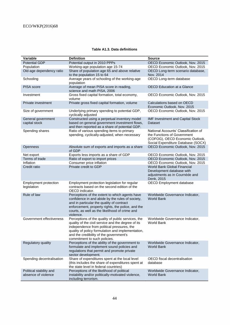
ECO/WKP(2016)68

44

Table A1.3. Data definitions

Variable Definition Source

Potential GDP Potential output in 2010 PPPs OECD Economic Outlook, Nov. 2015 Population Working-age population age 15-74 OECD Economic Outlook, Nov. 2015 Old-age dependency ratio Share of population age 65 and above relative

to the population 15 to 64 OECD Long-term scenario database, Nov. 2014

Schooling Average years of schooling of the working-age population

OECD Long-term database

PISA score Average of mean PISA score in reading, science and math PISA, 2006

OECD Education at a Glance

Investment Gross fixed capital formation, total economy, volume

OECD Economic Outlook, Nov. 2015

Private investment Private gross fixed capital formation, volume Calculations based on OECD Economic Outlook, Nov. 2015

Size of government Underlying primary spending to potential GDP, cyclically adjusted


General government capital stock

Constructed using a perpetual inventory model based on general government investment flows, and then reported as a share of potential GDP.

IMF Investment and Capital Stock Dataset

Spending shares Ratio of various spending items to primary spending, cyclically-adjusted, when necessary

National Accounts’ Classification of the Functions of Government (COFOG), OECD Economic Outlook, Social Expenditure Database (SOCX)

Openness Absolute sum of exports and imports as a share of GDP


Net export Exports less imports as a share of GDP OECD Economic Outlook, Nov. 2015 Terms of trade Ratio of export to import prices OECD Economic Outlook, Nov. 2015 Inflation Consumer price inflation OECD Economic Outlook, Nov. 2015 Credit ratio Private credit to GDP World Bank Global Financial

Development database with adjustments as in Cournède and Denk, 2015

Employment protection legislation

Employment protection legislation for regular contracts based on the second edition of the OECD indicator.

OECD Employment database

Rule of law Perceptions of the extent to which agents have confidence in and abide by the rules of society, and in particular the quality of contract enforcement, property rights, the police, and the courts, as well as the likelihood of crime and violence.

Worldwide Governance Indicator, World Bank

Government effectiveness Perceptions of the quality of public services, the quality of the civil service and the degree of its independence from political pressures, the quality of policy formulation and implementation, and the credibility of the government's commitment to such policies.


Regulatory quality Perceptions of the ability of the government to formulate and implement sound policies and regulations that permit and promote private sector development.


Spending decentralisation Share of expenditures spent at the local level (this includes the share of expenditures spent at the state level in federal countries)

OECD fiscal decentralisation database

Political stability and absence of violence

Perceptions of the likelihood of political instability and/or politically-motivated violence, including terrorism.


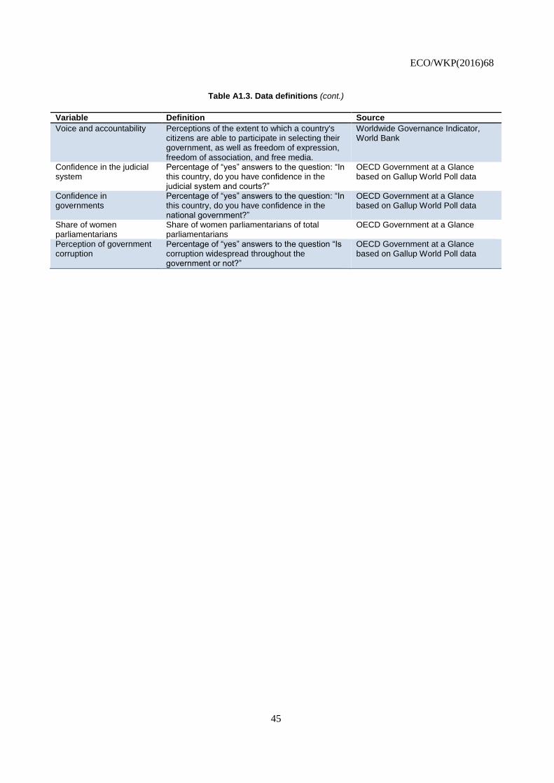
ECO/WKP(2016)68

45

Table A1.3. Data definitions (cont.)

Variable Definition Source

Voice and accountability Perceptions of the extent to which a country's citizens are able to participate in selecting their government, as well as freedom of expression, freedom of association, and free media.


Confidence in the judicial system

Percentage of “yes” answers to the question: “In this country, do you have confidence in the judicial system and courts?”

OECD Government at a Glance based on Gallup World Poll data

Confidence in governments

Percentage of “yes” answers to the question: “In this country, do you have confidence in the national government?”


Share of women parliamentarians

Share of women parliamentarians of total parliamentarians

OECD Government at a Glance

Perception of government corruption

Percentage of “yes” answers to the question “Is corruption widespread throughout the government or not?”


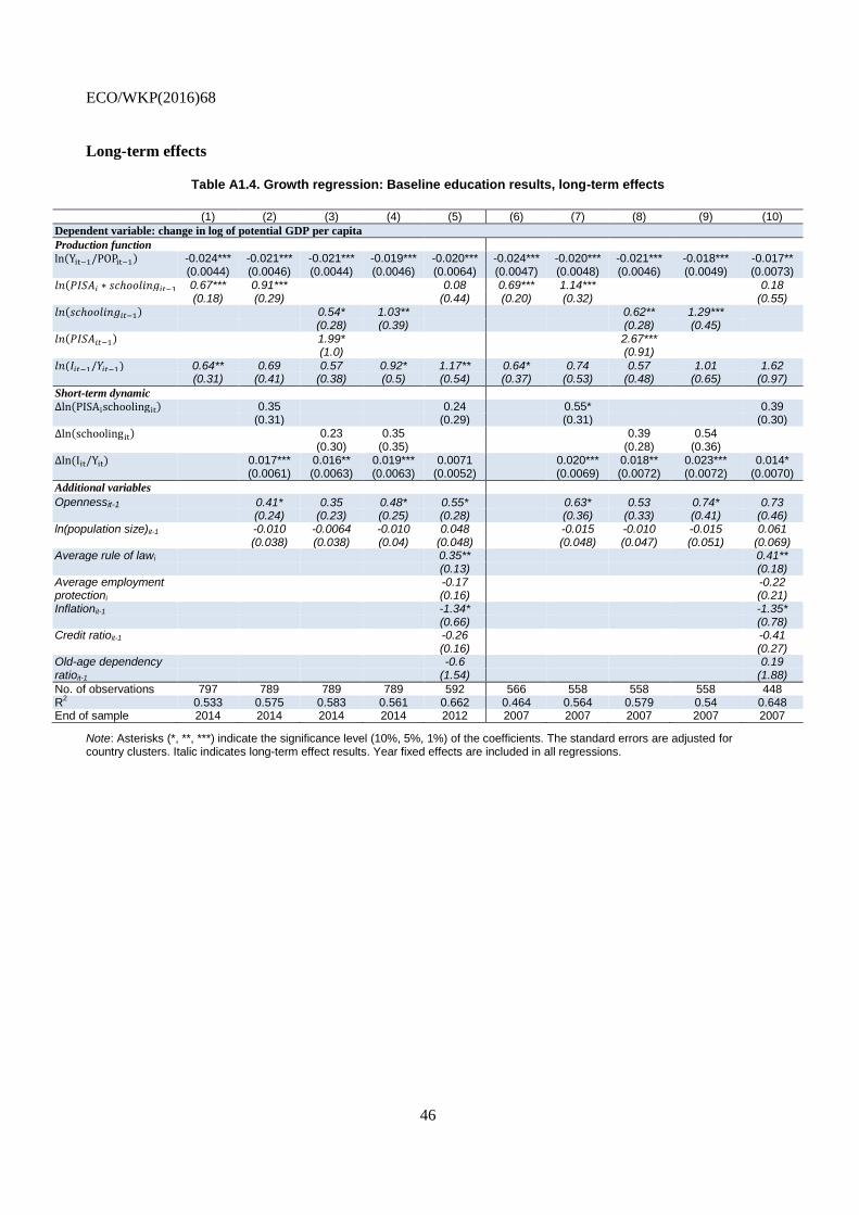
ECO/WKP(2016)68

46

Long-term effects

Table A1.4. Growth regression: Baseline education results, long-term effects

(1) (2) (3) (4) (5) (6) (7) (8) (9) (10)

Dependent variable: change in log of potential GDP per capita

Production function

ln(Yit−1/POPit−1) -0.024*** -0.021*** -0.021*** -0.019*** -0.020*** -0.024*** -0.020*** -0.021*** -0.018*** -0.017** (0.0044) (0.0046) (0.0044) (0.0046) (0.0064) (0.0047) (0.0048) (0.0046) (0.0049) (0.0073)

𝑙𝑛(𝑃𝐼𝑆𝐴𝑖 ∗ 𝑠𝑐ℎ𝑜𝑜𝑙𝑖𝑛𝑔𝑖𝑡−1) 0.67*** 0.91*** 0.08 0.69*** 1.14*** 0.18 (0.18) (0.29) (0.44) (0.20) (0.32) (0.55) 𝑙𝑛(𝑠𝑐ℎ𝑜𝑜𝑙𝑖𝑛𝑔𝑖𝑡−1) 0.54* 1.03** 0.62** 1.29*** (0.28) (0.39) (0.28) (0.45) 𝑙𝑛(𝑃𝐼𝑆𝐴𝑖𝑡−1) 1.99* 2.67*** (1.0) (0.91)

𝑙𝑛(𝐼𝑖𝑡−1/𝑌𝑖𝑡−1) 0.64** 0.69 0.57 0.92* 1.17** 0.64* 0.74 0.57 1.01 1.62 (0.31) (0.41) (0.38) (0.5) (0.54) (0.37) (0.53) (0.48) (0.65) (0.97)

Short-term dynamic

Δln(PISAischoolingit) 0.35 0.24 0.55* 0.39 (0.31) (0.29) (0.31) (0.30)

Δln(schoolingit) 0.23 0.35 0.39 0.54 (0.30) (0.35) (0.28) (0.36) Δln(Iit/Yit) 0.017*** 0.016** 0.019*** 0.0071 0.020*** 0.018** 0.023*** 0.014* (0.0061) (0.0063) (0.0063) (0.0052) (0.0069) (0.0072) (0.0072) (0.0070)


Opennessit-1 0.41* 0.35 0.48* 0.55* 0.63* 0.53 0.74* 0.73 (0.24) (0.23) (0.25) (0.28) (0.36) (0.33) (0.41) (0.46) ln(population size)it-1 -0.010 -0.0064 -0.010 0.048 -0.015 -0.010 -0.015 0.061 (0.038) (0.038) (0.04) (0.048) (0.048) (0.047) (0.051) (0.069) Average rule of lawi 0.35** 0.41** (0.13) (0.18) Average employment -0.17 -0.22 protectioni (0.16) (0.21) Inflationit-1 -1.34* -1.35* (0.66) (0.78) Credit ratioit-1 -0.26 -0.41 (0.16) (0.27) Old-age dependency -0.6 0.19 ratioit-1 (1.54) (1.88)


2 0.533 0.575 0.583 0.561 0.662 0.464 0.564 0.579 0.54 0.648

End of sample 2014 2014 2014 2014 2012 2007 2007 2007 2007 2007

Note: Asterisks (*, **, ***) indicate the significance level (10%, 5%, 1%) of the coefficients. The standard errors are adjusted for country clusters. Italic indicates long-term effect results. Year fixed effects are included in all regressions.

ECO/WKP(2016)68

47

Detailed regression results

Table A1.5. The role of public sector effectiveness

(1) (2) (3) (4) (5) (6) (7) (8) (9)

Production function

ln(Yit−1/POPit−1) -0.015*** -0.014*** -0.016*** -0.017*** -0.015*** -0.015*** -0.016*** -0.013*** -0.015*** (0.0048) (0.0050) (0.0044) (0.0040) (0.0040) (0.0047) (0.0046) (0.0048) (0.0040)

ln(PISAi ∗ schoolingit−1) -0.0052 -0.0078 -0.0076 0.010* 0.0021 -0.0072 -0.0013 0.0023 0.0021 (0.0060) (0.0079) (0.0075) (0.0051) (0.0050) (0.0055) (0.0055) (0.0055) (0.0073)

ln(Iit−1/Yit−1) 0.014*** 0.017*** 0.016*** 0.020*** 0.013** 0.014*** 0.013** 0.015*** 0.014*** (0.0047) (0.0045) (0.0049) (0.0053) (0.0054) (0.0047) (0.0051) (0.0051) (0.0049)

𝑷𝒖𝒃𝒍𝒊𝒄𝒔𝒑𝒆𝒏𝒅𝒊𝒏𝒈 Spending to GDP ratioit-1 -0.047*** -0.030* -0.036** -0.033** -0.038** -0.042** -0.028* -0.020 -0.033** (0.017) (0.017) (0.017) (0.012) (0.017) (0.016) (0.015) (0.015) (0.015)

𝑸𝒖𝒂𝒍𝒊𝒕𝒚𝒐𝒇𝒈𝒐𝒗𝒆𝒓𝒏𝒎𝒆𝒏𝒕 Government effectivenessi 0.0015 (0.0025) Government effectivenessi * 0.097*** Spending to GDP ratioit-1 (0.021) Regulatory qualityi 0.0041 (0.0033) Regulatory qualityi * 0.10*** Spending to GDP ratioit-1 (0.029) Confidence in the judicial systemi 0.00012 (0.000093) Confidence in the judicial systemi * 0.0021*** Spending to GDP ratioit-1 (0.00062) Spending decentralisationi -0.0082 (0.0061) Spending decentralisationi * 0.23*** Spending to GDP ratioit-1 (0.057)

𝑷𝒐𝒍𝒊𝒕𝒊𝒄𝒂𝒍𝒊𝒏𝒔𝒕𝒊𝒕𝒖𝒕𝒊𝒐𝒏𝒔 Political stabilityi 0.0012 (0.0016) Political stabilityi * 0.10*** Spending to GDP ratioit-1 (0.024) Voice accountabilityi 0.0047 (0.0034) Voice accountabilityi * 0.15*** Spending to GDP ratioit-1 (0.025) Share of women in parliamenti 0.000091 (0.000091) Share of women in parliamenti * 0.0032*** Spending to GDP ratioit-1 (0.00081)

𝑻𝒓𝒖𝒔𝒕 Confidence in governmentsi -0.000011 (0.000079) Confidence in governmentsi * 0.0025*** Spending to GDP ratioit-1 (0.00066) Perception of corruptioni -6.2e-06 (0.000057) Perception of corruptioni * -0.0016*** Spending to GDP ratioit-1 (0.00034)

No. of observations 547 547 547 461 547 547 547 547 547 R

2 0.769 0.756 0.766 0.808 0.771 0.776 0.763 0.758 0.768

Note: Asterisks (*, **, ***) indicate the significance level (10%, 5%, 1%) of the coefficients. Year fixed effects are included in all regressions. The standard errors are adjusted for country clusters. The long-run steady state coefficients can be calculated based on these short-run coefficients as ratios of the short-term coefficient to the negative of the convergence coefficient Ф. The short term dynamic and additional control variables are not reported to simplify the presentation. The indicators interacted with the size of government are perception indicators, which are strongly correlated within each other. The interacted variables are mean centered, which implies that the coefficients can be interpreted as average effects.

ECO/WKP(2016)68

48

Table A1.6 The effect of government size and public investment on the speed of convergence

(1) (2) (3)

Production function

ln(Yit−1/POPit−1) -0.015*** -0.015*** -0.013** (0.0054) (0.0049) (0.0051)

ln(PISAi ∗ schoolingit−1) -0.0052 -0.0077 -0.0065 (0.0073) (0.0062) (0.0065)

ln(Iit−1/Yit−1) 0.017*** (0.0048) ln(PrivateInvtit−1/Yit−1) 0.0080 0.0085 (0.0055) (0.0054)

Short-term dynamic

Δln(PISAi ∗ schoolingit) -0.24 -0.37* -0.33 (0.22) (0.21) (0.20)

Δln(Iit/Yit) 0.0089 (0.0059)

Δln(PrivateInvtit/Yit) 0.00049 0.00049 (0.0043) (0.0045)

Additional variables Opennessit−1 0.0079** 0.0081*** 0.0082*** (0.0029) (0.0028) (0.0026) ln(population size)it-1 0.00065 0.00074 0.00090 (0.00079) (0.00073) (0.00074) Averageruleoflawi 0.0029 0.0038 0.0037 (0.0025) (0.0024) (0.0025) Averageemploymentprotectioni -0.0025 -0.0026 -0.0026 (0.0026) (0.0021) (0.0021)

Inflationit−1 -0.0031 0.0082 0.011 (0.028) (0.021) (0.021)

Creditratioit−1 -0.0050** -0.0061** -0.0061** (0.0024) (0.0027) (0.0026)

Old − agedependencyratioi -0.020 -0.011 -0.017 (0.025) (0.022) (0.019)

Public spending Spending to GDP ratioit-1 -0.022* -0.0030 -0.025* (0.013) (0.013) (0.014) Public investment (share of primary spending) it-1 0.072*** (0.024) Public investment (share of GDP) it-1 0.21*** (0.062)

Public spending interacted with the past GDP per capita Spending to GDP ratioit-1*ln(Y it-1/POP it-1) 0.11*** 0.028 0.096*** (0.033) (0.030) (0.025) Public investment (share of primary spending) it-1*ln(Y it-1/POP it-1) -0.12*** (0.032) Public investment (share of GDP) it-1*ln(Y it-1/POP it-1) -0.37** (0.13)

No. of observations 547 547 547 R

2 0.757 0.783 0.783

Note: Asterisks (*, **, ***) indicate the significance level (10%, 5%, 1%) of the coefficients. Year fixed effects are included in all regressions. The standard errors are adjusted for country clusters.

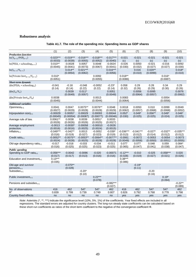
ECO/WKP(2016)68

49

Robustness analysis

Table A1.7. The role of the spending mix: Spending items as GDP shares

(1) (2) (3) (4) (5) (6) (7) (8) (9) (10)

Production function

ln(Yit−1/POPit−1) -0.023*** -0.019*** -0.016*** -0.018*** -0.017*** -0.021 -0.021 -0.021 -0.021 -0.021 (0.0033) (0.0039) (0.0055) (0.0052) (0.0040) (c) (c) (c) (c) (c)

ln(PISAi ∗ schoolingit−1) 0.010** -0.0028 0.0057 0.0048 -0.0024 -0.026 0.0050 -0.021 -0.016 0.0092 (0.0045) (0.0041) (0.0073) (0.0067) (0.0041) (0.030) (0.032) (0.027) (0.027) (0.030)

ln(Iit−1/Yit−1) 0.014** 0.021*** 0.016*** 0.016 0.020** 0.018* (0.0054) (0.0062) (0.0056) (0.010) (0.0099) (0.010) ln(PrivateInvtit−1/Yit−1) 0.010* 0.0092 0.018** 0.016* (0.0051) (0.0055) (0.0086) (0.0087)

Short-term dynamic

Δln(PISAi ∗ schoolingit) -0.041 -0.18 -0.048 -0.0052 -0.23* 0.058 0.29 0.28 0.34 0.29 (0.14) (0.14) (0.22) (0.22) (0.14) (0.32) (0.26) (0.29) (0.30) (0.26)

Δln(Iit/Yit) 0.0039 0.011* 0.0051 0.0056 0.0095 0.0076 (0.0049) (0.0057) (0.0049) (0.0064) (0.0057) (0.0062) Δln(PrivateInvtit/Yit) 0.0038 0.0013 0.0083 0.0054 (0.0045) (0.0044) (0.0064) (0.0056)


Opennessit-1 0.0041 0.0047 0.0075** 0.0076** 0.0048 0.0018 0.0050 0.010 0.0099 0.0049 (0.0027) (0.0029) (0.0028) (0.0028) (0.0029) (0.0062) (0.0057) (0.0068) (0.0068) (0.0052) ln(population size)it-1 -0.00029 0.00057 0.00029 0.00093 0.00044 0.052* 0.049* 0.056** 0.049* 0.046* (0.00045) (0.00054) (0.00087) (0.00077) (0.00046) (0.030) (0.025) (0.025) (0.024) (0.025) Average rule of lawi 0.0061** 0.0038 0.0039 0.0051* 0.0033 (0.0026) (0.0026) (0.0026) (0.0025) (0.0027) Average employment -0.0013 -0.0030* 0.00058 -0.00010 -0.0026 protectioni (0.0016) (0.0016) (0.0025) (0.0024) (0.0015) Inflationit-1 -0.049*** -0.042** 0.0013 -0.0052 -0.039* -0.036*** -0.041*** -0.027* -0.032** -0.035*** (0.016) (0.019) (0.027) (0.023) (0.019) (0.013) (0.012) (0.014) (0.012) (0.012) Credit ratioit-1 -0.0052** -0.0075** -0.0053** -0.0064** -0.0077** -0.0061 -0.0072 -0.0053 -0.0054 -0.0073 (0.0024) (0.0028) (0.0025) (0.0028) (0.0028) (0.0049) (0.0058) (0.0050) (0.0051) (0.0055) Old-age dependency ratioit-1 -0.017 -0.018 -0.033 -0.034 -0.011 0.077 0.077 0.048 0.059 0.084* (0.016) (0.025) (0.025) (0.023) (0.025) (0.065) (0.047) (0.041) (0.038) (0.047)

Public spending Spending to GDP ratioit-1 -0.056*** -0.0042 -0.0096 -0.020 -0.00071 -0.12*** -0.010 -0.025 -0.058*** 0.020 (0.017) (0.017) (0.013) (0.016) (0.016) (0.028) (0.019) (0.027) (0.021) (0.026) Education and investmentit-1 0.13*** 0.38*** (0.035) (0.086) Old-age and survivor -0.070** -0.19* pensions it-1 (0.028) (0.11) Subsidies it-1 -0.20* -0.20 (0.10) (0.16) Public investment it-1 0.22*** 0.19* (0.078) (0.094) Pensions and subsidies it-1 -0.082*** -0.22** (0.027) (0.089)


2 0.839 0.799 0.739 0.749 0.807 0.826 0.792 0.768 0.778 0.798


Note: Asterisks (*, **, ***) indicate the significance level (10%, 5%, 1%) of the coefficients. Year fixed effects are included in all regressions. The standard errors are adjusted for country clusters. The long-run steady state coefficients can be calculated based on

these short-run coefficients as ratios of the short-term coefficient to the negative of the convergence coefficient Ф.

ECO/WKP(2016)68

50

Table A1.8. The role of the spending mix: Pre-crisis estimates

(1) (2) (3) (4) (5) (6) (7) (8) (9) (10)

Production function

ln(Yit−1/POPit−1) -0.022*** -0.016*** -0.012* -0.015** -0.015*** -0.021 -0.021 -0.021 -0.021 -0.021 (0.0041) (0.0042) (0.0067) (0.0059) (0.0042) (c) (c) (c) (c) (c) ln(PISAi ∗ schoolingit−1) 0.014*** -0.00065 0.0084 0.0026 0.000072 -0.015 0.043 -0.011 -0.010 0.045 (0.0050) (0.0038) (0.0082) (0.0068) (0.0036) (0.032) (0.041) (0.040) (0.038) (0.039) ln(Iit−1/Yit−1) 0.014** 0.028*** 0.016** 0.015 0.030** 0.014 (0.0060) (0.0077) (0.0062) (0.0098) (0.011) (0.0092)

ln(PrivateInvtit−1/Yit−1) 0.0096 0.011 0.017** 0.025** (0.0059) (0.0067) (0.0080) (0.0099)

Short-term dynamic

Δln(PISAi ∗ schoolingit) 0.068 -0.086 0.047 0.018 -0.15 0.17 0.34 0.21 0.25 0.35 (0.15) (0.18) (0.25) (0.23) (0.17) (0.36) (0.34) (0.31) (0.34) (0.34) Δln(Iit/Yit) 0.013* 0.023*** 0.015** 0.014* 0.025*** 0.014** (0.0067) (0.0069) (0.0063) (0.0071) (0.0079) (0.0065) Δln(PrivateInvtit/Yit) 0.011* 0.0071 0.015* 0.016** (0.0060) (0.0056) (0.0082) (0.0073)


Opennessit-1 0.0043 0.0049 0.0079** 0.0086** 0.0049 0.0098 0.021** 0.022*** 0.020** 0.019** (0.0039) (0.0038) (0.0037) (0.0032) (0.0037) (0.0084) (0.0081) (0.0077) (0.0084) (0.0073) ln(population size)it-1 -0.0012* 0.00013 -0.00010 0.00081 -0.000083 0.00011 0.057 0.028 0.014 0.053 (0.00066) (0.00064) (0.00096) (0.00078) (0.00059) (0.036) (0.036) (0.038) (0.035) (0.033) Average rule of lawi 0.0049 0.0013 0.0034 0.0047* 0.00071 (0.0030) (0.0023) (0.0031) (0.0027) (0.0024) Average employment -0.0018 -0.0042** 0.00040 -0.0020 -0.0036** protectioni (0.0017) (0.0018) (0.0029) (0.0024) (0.0017) Inflationit-1 -0.037 -0.044* 0.0068 0.0033 -0.039 -0.029* -0.025* -0.0078 -0.020 -0.023* (0.023) (0.024) (0.030) (0.025) (0.023) (0.017) (0.013) (0.015) (0.015) (0.013) Credit ratioit-1 -0.0055* -0.0078** -0.0068** -0.0090** -0.0079** -0.0027 -0.0061 -0.0042 -0.0043 -0.0062 (0.0027) (0.0029) (0.0032) (0.0035) (0.0029) (0.0072) (0.0065) (0.0052) (0.0057) (0.0065) Old-age dependency ratioit-1 0.022 -0.013 -0.011 -0.0041 -0.0035 0.043 -0.055 -0.019 -0.0067 -0.031 (0.027) (0.030) (0.032) (0.030) (0.030) (0.056) (0.044) (0.031) (0.042) (0.040)

Public spending Spending to GDP ratioit-1 -0.029* -0.0019 -0.011 0.019 -0.0051 -0.043* -0.020 -0.0024 -0.017 -0.020 (0.016) (0.020) (0.015) (0.018) (0.019) (0.022) (0.019) (0.025) (0.020) (0.017) Education and investmentit-1 0.061*** 0.11*** (0.015) (0.031) Old-age and survivor -0.028*** -0.0026 pensions it-1 (0.0096) (0.038) Subsidies it-1 -0.11*** -0.16** (0.036) (0.077) Public investment it-1 0.12*** 0.070 (0.032) (0.041) Pensions and subsidies it-1 -0.033*** -0.041 (0.0085) (0.032)


2 0.840 0.785 0.722 0.749 0.800 0.852 0.816 0.802 0.807 0.819


Note: Asterisks (*, **, ***) indicate the significance level (10%, 5%, 1%) of the coefficients. Year fixed effects are included in all regressions. The standard errors are adjusted for country clusters. The long-run steady state coefficients can be calculated based on these short-run coefficients as ratios of the short-term coefficient to the negative of the convergence coefficient Ф.

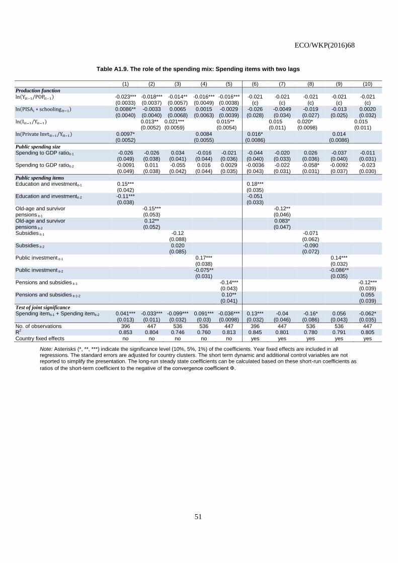
ECO/WKP(2016)68

51

Table A1.9. The role of the spending mix: Spending items with two lags

(1) (2) (3) (4) (5) (6) (7) (8) (9) (10)

Production function

ln(Yit−1/POPit−1) -0.023*** -0.018*** -0.014** -0.016*** -0.016*** -0.021 -0.021 -0.021 -0.021 -0.021 (0.0033) (0.0037) (0.0057) (0.0049) (0.0038) (c) (c) (c) (c) (c) ln(PISAi ∗ schoolingit−1) 0.0086** -0.0033 0.0065 0.0015 -0.0029 -0.026 -0.0049 -0.019 -0.013 0.0020 (0.0040) (0.0040) (0.0068) (0.0063) (0.0039) (0.028) (0.034) (0.027) (0.025) (0.032) ln(Iit−1/Yit−1) 0.013** 0.021*** 0.015** 0.015 0.020* 0.015 (0.0052) (0.0059) (0.0054) (0.011) (0.0098) (0.011)

ln(PrivateInvtit−1/Yit−1) 0.0097* 0.0084 0.016* 0.014 (0.0052) (0.0055) (0.0086) (0.0086)

Public spending size Spending to GDP ratioit-1 -0.026 -0.026 0.034 -0.016 -0.021 -0.044 -0.020 0.026 -0.037 -0.011 (0.049) (0.038) (0.041) (0.044) (0.036) (0.040) (0.033) (0.036) (0.040) (0.031) Spending to GDP ratioit-2 -0.0091 0.011 -0.055 0.016 0.0029 -0.0036 -0.022 -0.058* -0.0092 -0.023 (0.049) (0.038) (0.042) (0.044) (0.035) (0.043) (0.031) (0.031) (0.037) (0.030)

Public spending items Education and investmentit-1 0.15*** 0.18*** (0.042) (0.035) Education and investmentit-2 -0.11*** -0.051 (0.038) (0.033) Old-age and survivor -0.15*** -0.12** pensions it-1 (0.053) (0.046) Old-age and survivor 0.12** 0.083* pensions it-2 (0.052) (0.047) Subsidies it-1 -0.12 -0.071 (0.088) (0.062) Subsidies it-2 0.020 -0.090 (0.085) (0.072) Public investment it-1 0.17*** 0.14*** (0.038) (0.032) Public investment it-2 -0.075** -0.086** (0.031) (0.035) Pensions and subsidies it-1 -0.14*** -0.12*** (0.043) (0.039) Pensions and subsidies it-1-2 0.10** 0.055 (0.041) (0.039)

Test of joint significance Spending itemit-1 + Spending itemit-2 0.041*** -0.033*** -0.099*** 0.091*** -0.036*** 0.13*** -0.04 -0.16* 0.056 -0.062* (0.013) (0.011) (0.032) (0.03) (0.0098) (0.032) (0.046) (0.086) (0.043) (0.035)


2 0.853 0.804 0.746 0.760 0.813 0.845 0.801 0.780 0.791 0.805


Note: Asterisks (*, **, ***) indicate the significance level (10%, 5%, 1%) of the coefficients. Year fixed effects are included in all regressions. The standard errors are adjusted for country clusters. The short term dynamic and additional control variables are not reported to simplify the presentation. The long-run steady state coefficients can be calculated based on these short-run coefficients as

ratios of the short-term coefficient to the negative of the convergence coefficient Ф.

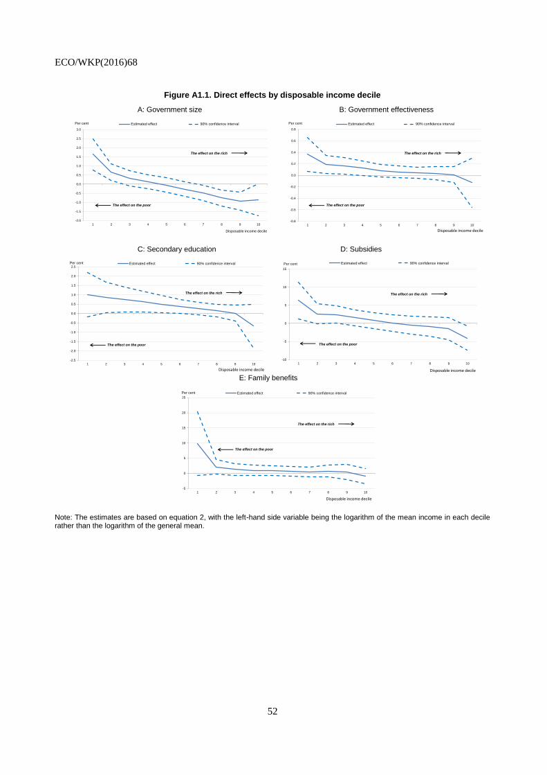
ECO/WKP(2016)68

52

Figure A1.1. Direct effects by disposable income decile

A: Government size B: Government effectiveness

C: Secondary education D: Subsidies

E: Family benefits

Note: The estimates are based on equation 2, with the left-hand side variable being the logarithm of the mean income in each decile rather than the logarithm of the general mean.

-2.0

-1.5

-1.0

-0.5

0.0

0.5

1.0

1.5

2.0

2.5

3.0

1 2 3 4 5 6 7 8 9 10

Estimated effect 90% confidence intervalPer cent

Disposable income decile

The effect on the rich

The effect on the poor

-0.8

-0.6

-0.4

-0.2

0.0

0.2

0.4

0.6

0.8

1 2 3 4 5 6 7 8 9 10





-2.5

-2.0

-1.5

-1.0

-0.5

0.0

0.5

1.0

1.5

2.0

2.5

1 2 3 4 5 6 7 8 9 10





-10

-5

0

5

10

15

1 2 3 4 5 6 7 8 9 10





-5

0

5

10

15

20

25

1 2 3 4 5 6 7 8 9 10





ECO/WKP(2016)68

53

Figure A1.2. Larger and more effective governments do not change market income inequality

Estimated direct impact of the size of the government along the income distribution

Panel B. Estimated direct impact of the effectiveness of the government along the income distribution

Note: The direct impact excludes any indirect impact of the change in policy on growth. Panel A shows the effect along the income distribution of an increase of the size of the government by one GDP point. Panel B shows the effect along the income distribution of an increase of government effectiveness by 0.01, where the government effectiveness measure ranges from 0.31 in Mexico to 2.17 in Finland.

-2.0

-1.5

-1.0

-0.5

0.0

0.5

1.0

1.5

2.0

2.5

-4 -3 -2 -1 0 1 2 3 4 5 6

Estimated effect 90% confidence interval Effect on the mean market incomePer cent



-1.5

-1.0

-0.5

0.0

0.5

1.0

1.5

-4 -3 -2 -1 0 1 2 3 4 5 6

Estimated effect 90% confidence interval Effect on the mean market incomePer cent



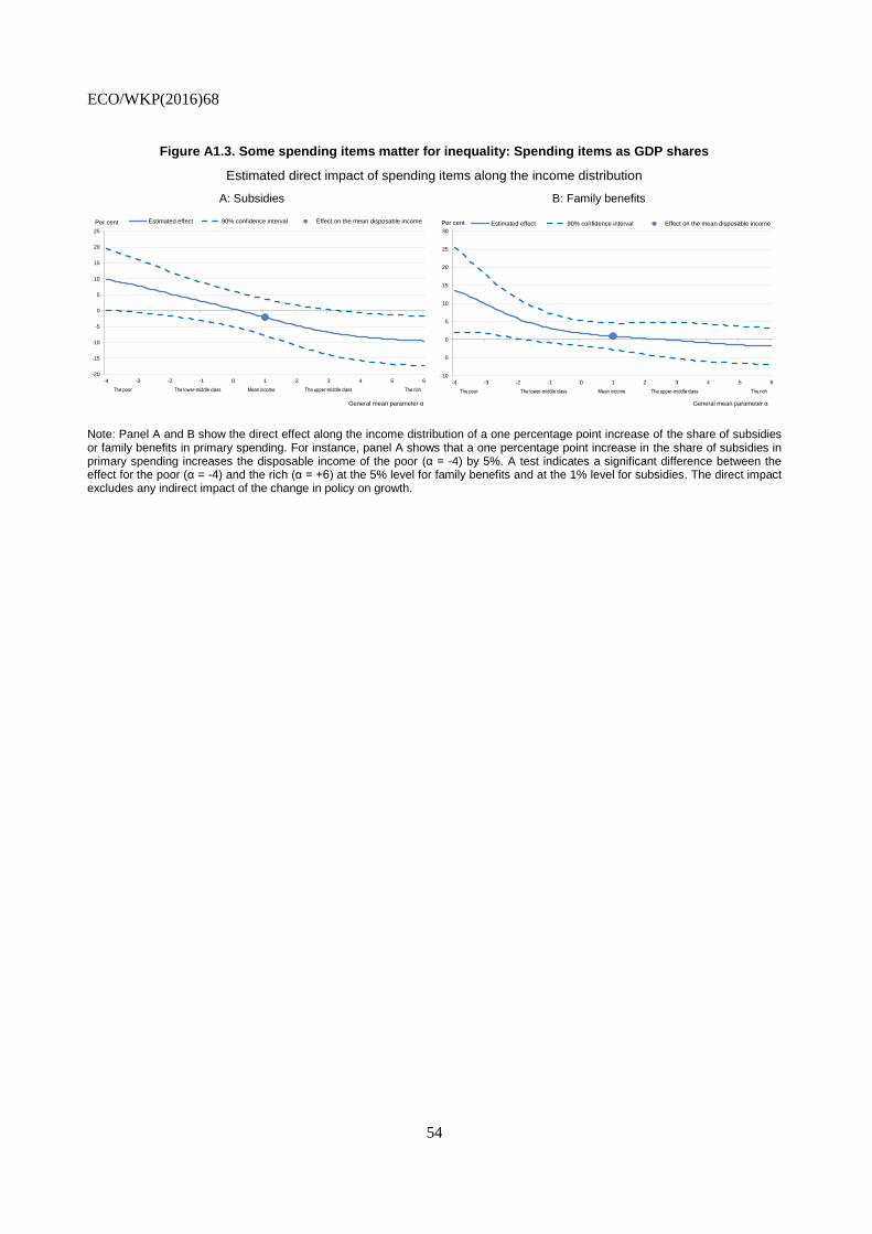
ECO/WKP(2016)68

54

Figure A1.3. Some spending items matter for inequality: Spending items as GDP shares

Estimated direct impact of spending items along the income distribution

A: Subsidies B: Family benefits

Note: Panel A and B show the direct effect along the income distribution of a one percentage point increase of the share of subsidies or family benefits in primary spending. For instance, panel A shows that a one percentage point increase in the share of subsidies in primary spending increases the disposable income of the poor (α = -4) by 5%. A test indicates a significant difference between the effect for the poor (α = -4) and the rich (α = +6) at the 5% level for family benefits and at the 1% level for subsidies. The direct impact excludes any indirect impact of the change in policy on growth.

-20

-15

-10

-5

0

5

10

15

20

25

-4 -3 -2 -1 0 1 2 3 4 5 6




-10

-5

0

5

10

15

20

25

30

-4 -3 -2 -1 0 1 2 3 4 5 6




Unclassified ECO/WKP(2016)68 - OECD.org · Unclassified ECO/WKP(2016)68 Organisation de...

Documents

Transcript of Unclassified ECO/WKP(2016)68 - OECD.org · Unclassified ECO/WKP(2016)68 Organisation de...