UNCLASSIFIED

AD NUMBER

LIMITATION CHANGESTO:

FROM:

AUTHORITY

THIS PAGE IS UNCLASSIFIED

AD837562

Approved for public release; distribution isunlimited.

Distribution authorized to U.S. Gov't. agenciesand their contractors;Administrative/Operational Use; 31 MAY 1968.Other requests shall be referred to DefenseAtomic Support Agency, Washington, DC.

NELC ltr 22 Aug 1974

■ -

r

A FORTRAN PROGRAM FOR MODE CONSTANTS (M IN AN EARTH-IONOSPHERE WAVEGUIDE

f <£>

00 00

<

f i

Interim Report No. 6*3

C. H. SHEDDY, R. PAPPERT, Y. GOUGH, and W. MOLER

trola and each

sr-r-«^--■■■■•■': NAVAL ELECTRONICS LABORATORY CENTER

SAN DIEGO, CALIFORNIA 92152

31 May 1968

Prepared for DEFENSE ATOMIC SUPPORT AGENCY on DASA Subtask RHA 2042 n n ^

NELC Problem M402 P .. JUL2 6 1968

L

O *>

3'

...

TABLE OF CONTEMTS

Abstract ...11

Introduction. 1

The Ionosphere Reflection Matrix 3

The Approximate Solution 6

Summary of Mode Parameters 7

Calculation of Radio Field Strength 11

Running the Program .....13

Appendix A. *..............2U

Program Listing .-....«« 26

References 58

FIGURES AND TABLES

Table A lit

Table B , 18

Table C 20

Table D 22

Table E 23

Functional Dependence Chart ........23

ABSTRACT

An updated version of an earlier waveguide program has been written In

the FORTRAN compiler language. The new program Includes the following

alterations or additions; (1) An Improved Runge-Kutta routine; (2) A

procedure which finds directly the starting solutions at the top of the

Ionosphere; (3) Provision for Including up to five charged particles;

(U) A method for economically finding approximate waveguide solutions;

and modifications for use of the program for ELF wave propagation.

11

I. INTRODUCTION:

This report is the latest in a series (1, 2, 3, kf 5, 6, 7) which de-

scribe computer programs which have been developed for calculating iono-

spheric reflection coefficients and/or waveguide modal parameters. All

earlier computer programs were written in the NELIAC computer compiler lan-

guage. This report describes a program written in FORTRAN 63 for the CDC

computer which solves the modal equation for propagation within an earth

ionosphere waveguide. The experienced programmer, familiar with the FORTRAN

language« should find it easy to make the necessary modifications for use of

the program in other computers.

The solutions of the modal equation are determined from the reflection

coefficient matrixes of the ionosphere and of the earth as seen looking up-

ward and downward from a position within the waveguide. The program system-

atically solves the modal equation for as many modes as are desired. The

propagation parameters, attenuation rate, phase velocity, and excitation

factor are determined for each solution of the modal equation. The method

makes full allowance for both earth curvature In the direction of propagation

and the orientation and intensity of the geomagnetic field with respect to

the path of propagation.

The reflection coefficient matrix of the ionosphere is obtained numerically

following methods developed by Budden (3). The ionosphere is described in

terms of the vertical distribution of charged particle density, the approp-

riate charged particle neutral particle collision frequencies as a function of

height, and the intensity, dip angle, and azimuth of the geomagnetic field.

As many as five charged particles of either sign and of arbitrary mass may be

included as constituents. At the option of the user the program may be used

to calculate and print a listing of the ionospheric reflection coefficients only.

In addition to the real constituents the medium contains a fictitious

linear distribution of permittivity extending to the ground which simulates

(takes into account) the effects of earth curvature.

The equations used for obtaining the reflection coefficient matrix looking

at the ground depend on the height at which the modal equation Is solved. If

the modal equation is evaluated below the ionosphere but above the earth, be-

cause of the linear distribution of permittivity, the surface reflection

coefficients are expressible in terms of solutions to Stokes* equation and

their derivatives. If the modal equation Is evaluated at the ground all

earth curvature effects are Included in the Ionospheric reflection coeffici-

ents and ordinary Fresnel reflection coefficients are obtained at the ground.

The ground conductivity is an arbitrary input so that results represent pro-

pagation over a realistic finitely conducting earth.

The modal equation is especially useful for calculating the effect on

elf, vlf, and If guided propagation by anomalous conditions such as caused

by solar flares or nuclear explosions. Step models or exponential models of

the ionosphere are often so unrealistic as to be virtually useless for eval-

uating the effects of such anomalies. The present program calculates the

attenuation, phase velocity, and excitation of important waveguide modes for

realistic waveguide parameters. The program thus allows one to make realistic

estimates of changes in field strength and phase velocity over critical paths.

In summary, the physical input parameters for the waveguide program are:

1. The azimuth of propagation with respect to the horizontal component

of the geomagnetic field.

2. The geomagnetic dip angle and field strength.

3. Hie radio frequencies.

k. Vertical profiles of up to five charged species (electron, positive

and negative ions).

5* An exponential but otherwise arbitrary collision frequency distribution

with height for each specie of charged particles.

6. Hie ground conductivity and dielectric constant.

The output can be either a printout of the reflection coefficient matrix

of the ionosphere at desired height Increments within and below the ionosphere

or, by using the complete program, the waveguide mode parameters for as many

modes and radio frequencies as desired.

■

II. THE IONOSPHERE REFLECTION MATRIX

A. Exact Solution

The Ionosphere reflection matrix, re , at height, d. Is obtained by a

numerical Integration of differential equations given by Budden '. The

differential equations are of the form

2i*-f+s'\-&sc*-sr% (n-i)

where /V-/

Because of some symmetry In the elements of the S-matrlx, It may be written In the form

S|i a + Su b -Si

-s 2.1

M2

'Zi

-cii,a-d,ib du

where

Sua' • Tu +T*4 dna» ' Tn -TH Sub- ̂ T4>6 - CT4, dub- • Tf4/C-CT* SiZ • • WC + T42 diz » • 1.1/0-141 Sv • • w:+T3, du • • Ts4/C-TSI Sax • - c+vc du ' ' C-Tsz/C

-cia -du

6/iCX'jiib

(II-2)

where C » cos 0 and 6 Is the complex angle of Incidence. The T-matrlx Is

of the form

/

z- 0

V where

SmatD

0

C+na^- rn^m Jj

0

I

o

0

^

0 (II-3)

S s sin 0 (II-^)

and

^^ü^

X \

iYiu -YxYy

-i^-YxY.!

-iY,u-xyy i tp-yxya

w _ yUpg I"!» V and (^fe In opposite direction for

' mco

*■ CO

a - i-il £o ~ electric permittivity of free space li =■ magnetic permeability of free space Lf s geomagnetic field

CO = angular wave frequency

The quantities N, e, m, v (nu) have different values, at a given height,

for each species. The quantities are

N » species density e = charge of electron or of lun (negative for electrons and negative Ions) m ■ mass of electron or of Ion ^)= collision frequency

For each species there vlil be an MK,. The matrix,^, used In computing the T-matrlx Is then

*-J tRh (11-5;

The differential equations are Integrated by the Runge-Kutta technique,

starting at some height above which negllgeble reflection Is assumed to take

place. Error control Is by means of a comparison, for each step, uf the

Increments In the elements of^ computed with the fourth order Runge-Kutta

method, and that computed vlth a second-order Integration step. Although not

a completely rigorous error test. It has been found to be very reliable.

The eight Integration variables are the arguments and the logs of the

magnitudes uf each of the four elements of the reflection matrix. The

derivatives of these variables are obtained vlth the expression

(H % (II-6)

i where log Kii Implies the complex logarithm of the ii tk element of ^,

It turns out that the Initial conditions for the Integration, I.e., the starting value of ^R, Is the value of ^ for a sharply-bounded Ionosphere with properties corresponding to the Ionosphere at the top of the given electron

density and collision frequency profiles. The solution used Is that described (9) In a paper by C.H. Sheddy, x .

B. Approximate Solution

Most of the running time of the NELC waveguide program is in the compu-

tation of ^ which is used in the modal equation jj^J^^ -1=0 ,

Since the eigen values of e usually occur along a line in the complex e-plane,

it often suffices to compute R for two or three values of e and interpolate s*-*

between these values to obtain R = f(G). In this way the total run time is

cut to a fraction of that for the exact solution.

Approximate solutions may be used for exploratory work where one does

not require great accuracy. It may also be used in cases where the electron

density profile Itself is not known too well, since the errors resulting from

use of the Interpolation may be no greater than the uncertainties due to not

knowing the profile too well. Even when exact solutions are desired, approxi-

mate solutions may be obtained first as starting values for exact solutions.

The Lagrange interpolation polynomial is used in the program:

where log R Implies the complex log of an element of ^R. R. is a value computed

with the full-wave solution at the angle, ö,.

The user must select n values of 9. when using the approximate scheme.

Three or four values of ek generally give best results, often two suffice.

For best results these should be chosen as being in a line in the complex 0-

plane roughly approximating the line along which the eigen solutions are ex-

pected to be. It also has seemed best not to have more than one 0. with the

same value for the real parts or the same value for the imaginary parts.

When using the waveguide program for the first time, the user might try

several sets of 0. for the same set of input data in order to gain a feel for

the sensitivity of the approximate eigen solutions on the 0, .

•

10 III. SUMMARY OF RODE PARAMETERS

Following the formalism developed by BuJden, "^ whereby one wtrks within

the framework of a planar stratified medium and includes earth curvature via

the artifice of a modified refractive index, it is well known that the mode

equation may be written as the determinantal equation.

FD(e) = IRpCe)Rp(e^ - i| = O (m-i)

where RDCO) (III-2)

is the reflection matrix looking up into the ionosphere from height D and

RD(©) -

/

.iKWe)

V 0 .RIDC©)

(III-3)

/

is the reflection matrix looking down from height 0 towards the ground. The

angle, 9, is the angle of incidence at height z = H where the modified index

of refraction

n^ /-oc(H^) (III-U)

is unity. The full wave equations programed for the purpose of determining the

elements of KpC©) are ^iven in section II, It is emphasized that earth curva-

ture is included In the calculations of the elements r\,©(€t) # by the suscepti-

bility matrix. Since K-odSy is assumed to be diagonal it is essential that the

level D be chosen at or below the base of the ionosphere. Except for D - 0 and

some ELF calculations, KD, IS calculated as described in reference in

terms of solutions to Stokes* equation and their derivatives. The solution to

Stokes* equations which we have chosen to work with are the modified Hankel 12

functions of order 1/3 as defined in reference . It should be observed that

the latter functions are linearly related to the perhaps better known Airy

functions. When D = 0 or when the magnitude of the hyperbolic sine of the

imaginary part of the eigen angle exceeds a preassigned limit, the K.p^ matri>

is calculated directly from the Fresnel reflection formulas.

The principal objective of the present work is the solution of (1) for the

eigen angles, 9 . To achieve this the well known Newton's method is used. The

procedure is to guess a solution do to the equationr^)(0)-O. The function FDC©)

is then reevaluated for 0« + §d and the correction to da found from the equation

AG - - F(e) ^© (III-5)

F(©o+ S©)-r(e.)

The correction determined by Eq. (5) is then evaluated and the process re-

peated until the quantities lA©r| and |A0i| are reduced to within a

preassigned tolerance. For the first iteration the value of ^9 is taken

equal to 0.01*. The subsequent choices of ^0 are contigent upon proximity of

the results of the last two Iterations.

With the eigen angle, 0 , for mode n determined the following mode para-

meters are readily evaluated

phase velocity at the ground ■ c Jwi K (sin 0^), 5iu;

(1X1-6)

attenuation constant at the ground = "^'bSS^JiK isiflQ / /yP (in-7)

8

excitation factor as defined by Wait =

.^'^ (l^fe&Rj^ "T " "laei., 'M.

Mode mixing parameter (printed out as polarization) «

lllN»li.l<M

where \C * 0 + "H/Z)

(III-8)

(III-9)

(111-10)

f. e^-f; RM30+MM" f.hXq^) +i:ifi2toc)

(ni-ii)

.% » i..!4 Ü '-fe.)^f )\^)-»^(#) (WJ-5?Ä)i/^)]

Ft- (^H^Ä^-i^)^- Stn,U?-A,(^]

(111-12)

(III-13)

i square of the complex index of refraction of the ground

^ijWö'v-^H-ZJ)

(lll-HO

(III-15)

The subscript r in Eq, (6) implies the real part while the subscript i in

Eq. (7) implies the imaginary part. The subscript on q represents the value

of z at which q is evaluated. For example, q» means that Eq. (15) is to be 2

evaluated for Z =0. Similarly, the subscript in n represents the value of Z

for which Eq. (k) is to be evaluated. The functions h, and h2 are the modified

Hanlcel functions of order 1/3. The primes in Eqs. (12) and (13) denote de-

rivatives with respect to the argument. The quantity h* which occurs in Kq. (8)

is called REPL HT in the program and has been introduced solely for the purpose

of normalizing the excitation factor for the vertical dipole in a way which is

consistent with Wait's definition v . Closely related quantities also in-

cluded in the print out are termed EXTRA MAG and EXTRA ANGLE. These quantities

are simply the mamitude and argument of the right hand side of Eq. (8) with

the factor (-i —T" ) divided out. The quantities EXTRA MAG and EXTRA ANGLE are

used in conjunction with the mode sum analysis discussed in section IV. The

quantity printed out as polarization, that is the right hand side of Eq, (9),

is in fact not a measure of the polarization but as shown in reference ih is

very closely related to the ratio of the vertical to horizontal components of

polarization which comprise each mode under the general condition of an aniso-

tropic ionosphere. The right hand side of Kq. (9) becomes meaningless under

conditions of an Isotropie or near Isotropie ionosphere. For then the numerator

of equation (9) is very small because of a small conversion coefficient. On

the other hand the denominator of Eq. (9) even for a vertically polarized mode

will not vanish in general because of round off error so that the entire ratio

is then dependent upon round off error and In fact can have magnitude less than

unity even through the mode Is vertically polarized.

Finally, the quantity printed out under the label THETA PRIME, is simply

the value of the eigen angle at the ground (recall that the eigen angle which

results from the process of interation is referred to height H).

10

IV. CALCUIATION OF RADIO FIELE STRENGTH

For the frequencies considered for waveguide propagation the transmitting

antenna Is generally a vertical monopole above the surface of the earth. Be-

cause the earth Is a good conductor the radiation characteristic of the antenna

Is virtually that of a dlpole radiating Into a half space. The power radiated

Pr Is then

n - ibo-xHitl w waHs (IV-1)

where I Is the rms current, 1 Is the effective height of the antenna and X Is

the radio wavelength. The electric field at a distance D from the transmitter

for the n th mode can be written as:

[-JeDO-^)] &ism%en V/m (IV-2)

where T7 Is 377 ohms, c is the speed of light, f Is radio frequency, a Is the

radius of the earth, C Is the cosine of 0 the n th eigen angle, k Is wave

number, and x In the magnitude of the exltatlon factor (extra mag.). A

practical form to use Is

-C, Eir/m/Kw) = Ci e

where

(IV-3)

and a ■ attenuation coefficient In db/megameter.

The relative phase of the signal (relative with respect to free space pro-

pagation or to a local oscillator) Is given by

11

(p -. M. J)(l -£)+<po dv-M

where 9 is the relative phase at the receiver, c is the speed of light, V is

the phase velocity and cp« is the argument of the excitation factor in radians.

12

s

V. RUNNING THE PROGRAM

A. The profile deck(8)

The program, whether run for WAVEGUIDE SOLUTIONS or for REFLECTION

COEFFICIENTS can be run with or without Ion density profiles. The profiles

are set up the same way for either case. The electron density profile comes

first and Is preceded by a SPECIES I PROFILE card and an alpha-numeric card

punched with Information needed to Identify the run. The profile starts at

the top of the Ionosphere and contains the height In kilometers and the

electron density/cubic centimeter for that height. The height Is punched In

columns 2-7 and' the density Is punched In columns lU-21, The decimals are In

columns 5 and 15. If an electron density of zero Is used the program will -40

change It to 10 . Although the program Is often run with an electron den-

sity for every half kilometer. It may be run using only the significant

heights. For example, only two cards are needed for an exponential profile:

One at the top and one at the bottom of the profile. The program Interpolates

in a straight line between the logs of the densities and heights given in the

profile deck. The profile deck ends with a card punched with nines in the

first 8 columns. If the program Is to be run without ions, the input para-

meters immediately follow this nines card. If the program is to be run with

ions, this nines card is followed by a SPECIES 2 PROFILE card, another card

with identification, then the top of the positive ion density profile and so

on. This also ends with a nines card followed by a SPECIES 3 PROFILE card,

an identification card, and the negative ion density profile. Again a nines,

and then the input parameters. However, since the negative ion density is

equal to the positive ion density less the electron density for each height,

the program will calculate the negative ion density if a NEGIONS card is

placed at the end of the positive ion density profile. The ion density pro-

files must have the same heights as the electron density profile. A sample

profile with ions included is shown in Table A.

B. Waveguide Solution Input Parameters

The input parameters are placed anywhere on the card but according to the

following format. The names, e.g., MAGFIELD, must have no spaces between the

letters. The name is followed by one space, an - sign, another space, and then

the value of the parameter. If a parameter has more than one value they are

listed on the card or on following cards with one or more spaces between them.

The parameter name is only used once.

13

Table A

SD«-r «->; : ^hürii F 5^iPLC fK Kfllf PU-CTK'^i I'F -.'«.ITY

l*:r.( 0 '.1H^♦HA g«" on •..Q2f-*n^ vJ'-» , 00 H .<*2i:*fi< ■sc on l.r?6M*n? H''. , On 1 .7?f-*ns 7r on :>.42^*ni 7! •m ?,«5t**n!:' ^c no ''.^.sr+ns An M.i " .73^*f:* cc r.n l. A *• p ♦ n <t -.r f il *•!. F. 1 ^ ♦ fl .^ ^«" r r. '.o?t»n? ';'1 CP 'i,fi6^*R<i ?K I'D ^.^^.t-' + n^ •»i1 (•n ? .^v«-*C!2 i ro ;>. A 4 ^ ♦ n i ?'• f-n v'.o?c*rt 1 c f'O ?.riijK-Pi lr 00 ^.j7f--r>

1" ro H.«7c-nf.

^.r7p-Pf, 90<>r.QGgg

SPflf-S i pporiLP S«MH.P ppnHLP POMTlvt irM IiEN«:iTY inn.f.Q M.18^*n< y.no (S.OTC^P* V'.nri t..03«-*n« Br.i n 1 .?7t-*rh P ^ . " 0 i .78P*r5; 7e ,0* '•.^(-■♦n^

7fM 0 4,?6P*nt A p. r ■ n 7.R9P*nf f.^.ÜÜ i.4iP*n6 5r.''0 ?.?5»-*nt 5n,f.O ?.f>9^*{\t -«c. n ft ^.10^*06 - ^ . i' 0 ^,4V?*n6 3B.f>0 3, 76F-*n6 3r.''0 ^,vi^*r.b 2^,ro ?.?.?e*üt gp.cn f.7tii-*0b 1* .1 0 1 ,?fi^*n?;' IC.ffi ^,16^*nä ^.00 4.47fr*f'v n , cp s, ^v^^r:-

ycQrycgv NP-iTi ,vS

14

The approximate method will find up to 25 solutions in 10 minutes and

the exact method might find one solution in that amount of time. Therefore

it expedite.- the search for mode solutions. Often these solutions are

sufficiently accurate for the purpose. If this is not the case they can

serve as excellent starting solutions when running the exact method. To

set up an approximate run, only two cards must be added to an exact waveguide

run. These are the RPOLY card and the TUST card which are explained below.

AZIMUTH is the direction of propagation in degrees, measured east of mag-

netic north. West-to-east propagation corresponds to an azimuth of 90* and

east-to-west propagation corresponds to an azimuth of 270°.

DIPAICLE is the magnetic dip angle in degrees, measured from the vertical

and Is always between 0 and 90 degrees for propagation in the northern himis-

phere and between 90 and 180 degrees for propagation in the southern hemisphere.

MAGFIELD is the intensity of the magnetic field in Webers/square meter.

Use 0.0 for no mag field.

COEFFNU and EXPNU are the values used to find ^) , the collision frequency

where

-j) = COEFFNU x exp (EXPNU x Z)

and Z Is In meters, EXPNU is in inverse meters and COEFFNU is in collisions/

second. If ions are included, a separate collision frequency is needed for

each species and is listed on each card in the order of the profiles. For

example COEFFNU ■ U.3O3EII I.O76EIO I.O76EIO would mean that the coefficient

of the collision frequency is 4.303EII (^.303 x 10 ) for the electron density

profile and I.076EIO for the two ion density profiles.

EPSILON and EPSILONO are the permittivities of the ground and free

space respectively and are to be expressed in units of farads/meter.

D is any height below which ionospheric effects can be considered neglig-

ible and must be consistent with the bottom of the profile deck. Care must

be taken in satisfying the preceding condition. If there is doubt as to

whether a suitable value has been chosen, it is advisable to run the program

to different heights, D, to verify that the eigen-angles have stabilized.

Generally, stability to better than + 0.05' In the ground eigenangle is ob-

tained.

15

H is the height, expressed in kilometers, which represents physically

the height at which the modified refractive index becomes unity and is the

height at which the unprimed eigenangle is measured. Theory, good to first

order in the parameters h/a and z/a, predicts that the final ground solutions

are independent of H. However, investigation has shown that the results vary

somewhat when H changes from 90 Km to the ground (by approximately a tenth of

a degree in the ground eigen angle). This variation is attributed to higher

order effects in the earth curvature correction. Although contributing to some

uncertainty in the final results, these variations can be considered small and

are sufficiently accurate for most purposes. Generally, It Is sufficient to

choose both D and H to be the height on the last card of the electron density

profile,

ALPHA is in Inverse kilometers and is equal to 2/{earth's radius in kilo-

meters). If flat earth programs are run, a very small number (e.g, 10' km' )

should be used Instead of zero,

RELPREC is a parameter which helps determine how accurately the calculations

are to be done, A RELPREC of 1,0 would be fast but not very accurate, 2,0 is

usual, and 3,0 or k,0 would give about maximum accuracy,

SIGMA is the ground conductivity expressed In units of mhos/meter.

REFLET is chosen to be a reasonable estimate of where reflection takes

place. It Is used in both the approximate and the exact methods as a factor

in obtaining WAITS EXCITATION FACTOR. It is also used in obtaining the approxi-

mate solutions. It Is in kilometers.

FREQKHZ is the radio frequency In kilohertz/second.

THETAINC is a card used to control the iterations. A THETAINC of 1,0

Insures that each succeeding iteration will be no more than one degree (In

real and In imaginary parts) from the preceedlng one. This keeps the program

from arriving at a solution other than the one desired. However, if little

is known about the eigen angle solutions, a THETAINC of 5.0 or even greater

would be best,

MRATIO is used only when ions are Included, The first number Is unity;

the second the ratio of positive Ion mass to electron nass; and the third, the

ratio of negative Ion nass to electron mass,

CHARGE is also necessary only when ions are Included. The first number is

the charge of electrons, -1.0, the second, the charge of positive Ions, + 1.0,

and the third the charge of negative ions, -1.0.

16

RPOLY = 1 If approximate solutions are desired.

TUST Is a list of complex angles used In the approximate method to

obtain exact reflection coefficients vhlch are vised in an Interpolation

scheme to find the elgenangles of the problem. The closer the elements of

the TUST are to the final eigen angle solutions the closer the solutions

will be to exact solutions. For example, If all modes were derived between

70* and 80°, the TUST might look like the following:

TUST = 70 -3 75 -2 80 -1

Then all eigens in that range could be run in very little computer time.

E.g. the EIGEN card might appear as

EIGEN = 70.6 -2.7 73.5 -1.2 7^ -1 78 -2.5

If that is not accurate enough, and an approximate solution near (76, -1.6)* is

desired the TUST might look like the following:

TUST = 75 -1.8 76 -1.6 77 -1.1»

EIGEN precedes the trial eigen angles. As many eigen angles as desired

are punched on cards in the ^ormat of real part. Imaginary part, real part,

imaginary part, and so on. Each number separated by one or more spaces. If

more than one card Is needed the numbers are Just continued on the following

cards without revising the same EIGEN.

WAVJ2GUID is the command to the computer to start and complete the wave-

guide solutions.

Sec Table B for a sample approximate waveguide run with ions included.

These parameters would follow the profile decks. For the run to be the

exact method, only the RPOLY card and the TUST card need be removed.

C. Reflection Coefficient Input Parameters

FREQKHZ (See Waveguide input parameters)

AZIMüra "

DIPANGLE "

MAGFIELD "

COEFFNU "

EXPNU

D

H

ALPHA "

RELPREC "

17

Table B

A7IMUTH r fc3.n DTP/u.ftLF = 17 C MARflPLD = 5,nE-(!c

COgrp ,1 s 4.3C'3F11 l.C7fcF-in 1.&76P10 EyPMU a -1.62PE-04 -1.6r:?E-04 -1.62?E-04 EPSriON ' 7.172Ö1(?4F-10 PPSIL^NO = 8.R5434P-1? U s o.n H s n.o Al.P^A a 3,14E-C4 RPLP^C * c.O STr,>A s «,.64 RPFI HT r (Sn.C MPATin = i.o SRCfO.C t;fcOOC.O nUAPfiP « -1,0 l.n -1.0 TMETA!MC s l.C RPfU Y « 1 tl If T « 7«^.? -7.0 8?.0 -Ü.O 08.S -1.0 FT3P^ « 7?.Ct -2.L 7^.0 -?:.0 77.P -2.0 7«.0 -2-0 79.1 -?.0 80.0 -2.0 8?.o -2.C 03.1 -2.0 fc4.o -2.C «5.0 -2.0 8^.0 -2.0 87.0 -2.0 M.T -? 87.^ -2.( bH.5 -2.0 6w.5 -2.0 PPprKt-Z - IF.O rtAVf-r;|.Iü

18

MRATIO (If Ions are in- " eluded)

CHAHGE " "

TSETA Is the complex angle of Incidence in degrees.

See Table C for a sample input for reflection coefficients for electrons

only. The reflection coefficient program only runs exact.

RC is the command to the computer to start and complete the reflection

coefficients,

D. Linking Several Computer Runs

By doing several different runs in one computer input one can sometimes

save on turnaround time and cut down on card duplication of either Inputs or

profiles.

More than one data deck is run at a time by following the WAVBGUID card

with a SPECIES 1 PROFILE card and so on through the profile or through the

ion profiles as before. Doing this clobbers the profiles which were originally

in the computer but all the other input remains as it was. At the next WAVE-

GUID card the program starts on this "second" program. If any changes in input

parameters were desired on this second run, they would be changed between the

profile and the WAV3GUID card. For example, if D = 0.0 on the first profile

and 0 ■ 65.O on the second, the new profile would end with a nines card and

then NBGIONS, if ions were included, then D = 65.0 and then WAVEGUID.

Changes in the parameters for the data deck are stated between WAVEGUID

cards. All other inputs would remain unchanged. For example, if several mag

fields are desired for a given profile and set of parameters, only mag field

would be changed before calling WAVBGUID again. For example

MAGFIELD = U.OE-05

WAVBGUID

MAGFIELD =0.0

WAVBGUID

It is sometimes Justifiable under disturbed conditions such as SID's or

man-made ionization anomalies to neglect the influence of the earth's magnetic

field. The modal equation then factors into a product, one factor of which

contains solutions for vertical polarization, while the other factor contains

solutions for horizontal polarization. A provision is thus made whereby under

those circumstances either the vertical or the horizontal solutions may be

obtained independently. Of course for vertical dipole excitation, the verti-

cally polarized modes ar^ the physically meaningful modes. '30 when vertical

modes are desired and the profile is run with no maß field, the comnand TYPEITSR-1

19

~ , ...... ,.·

Table C

so~~I~S 1 PRJFILE Si~~l~ PRnFtLE ~L~CTH0NS n~LY tJn.no 7,02~ 04 . ~~-. uu .1. rj M= o 4

9~.~0 1.33~ 04 R~.OD ~.12~ n3 ~n.no ?.Rn~ n3 ?~.00 1.34~ OJ 7n,r)q c;,72.: 02 ~~.o~- ~~~'~ n~ 61l,OQ "S'!),OQ 5 ::1 .00 4c:,oo 4'1,(10

·-·-3~. cnr 3("1,0i) 21? • n :J 20.0f'J tc:;.or> l!'l,OI) - ·~; (fi) -

o.oo 9990~()99

-~.401: 01 6.?0~ Ob 4,?7~-01 1.6()1,;-01 5.421=-n;: :!_.58~-02

4.03~-03 Q,?41=-04 2.19~-04

">.32~-05

t.47~-n5 s·.na~-ao (}.('('~ 00

47t~UTt-~ : 33,:) DT~Ai\Jr.:LE ~ 17,;) MAG~l~LO : 5.0=-o~

-·- -··~:·v;r.,tJ =--1. 62?~-04 -· C l"' i; ~=" P' U = 4 , 3 I) 31711 D ·= l),f)

H : 1),0 Al..~!-iA : 3,14E•J4 RI=LPRFC : 2.0

· ·· r~~~~~2 = i~:b T~ETA : 9~.5 -1.5 Rt

will force only parallel solutions. If desired, horizontal solutions only

will result from the command TYPEITER = 2. Either command may be used when

propagation E-W or W-E is run at the geomagnetic equator (I.e. propagation

direction transverse to the magnetic field),

E, Waveguide Solution Computer Printout

Line Explanation of Table D

1, 2 Real and Imaginary parts of the eigen angle followed by their reflection coefficients.

3 Difference between final two eigen angles.

k Real and imaginary parts of the F function. See III.

5 Phase velocity of mode at the earth's surf act.

6 Phase velocity divided by the speed of light.

7 Attenuation of the vertical E-field in dB/1000 km at the ground.

3, 9 Magnitude and angle of Wait's excitation factor which has been normalized by dividing out the -ikh'/2 term.

10, 11 Wait's excitav.ion factor explained in (8). These excitation factors are for a vertical dipole antenna. See III-8.

12, 13 These give an indication if the eigen angle is horizontally or vertically polarized and are explained in III-9.

lh The eigen angle at the ground.

F. Reflection Coefficient Computer Printout

Explanation of Table E.

The computer prints out the height first then across the page, the modulus

and argument in radians of „R,, , XRA , XR„ , „R^ . At the bottom of the

printout it prints XRM / J^ and xet, - .9^ .

21

Table D

ac OOM • • • K» or tiiut « « « w*m «» OD OH* • •

ir w e »-• MO;»

m m « wt I »

I

v< e c en v4 ac • • <o>ro • u. ui ir <« ac 10 o«« « IT v« • • cn « CM »

KM .«4 •1 *«M < <4 ■ • et « «v

I «H

I ^

ir in «(CM o o al*4

«-< » • «« •4 Ul IM Ottf\

«4C OC\J MV • -

mm «•« o o air » • arg

>(M

» » It* o

ac

to

«

H M

t3

N i» C9

■

(k ooa»

IMC «i» *> CM - - UN •«• O MO T4

O C Q O O

e *4v>m oajm N

ui ui^ w r» Äo« M« • • » <• «4 a its ♦! ^.

«4 OKtl

» U> Ui

o cä«i» -SI «i

t

IT ml o a

e»

SSj

>l

•sä t t

111 Ul wr«. » e iv • » •

m •

o», »4MI an OCM am

tun UJUJllV « CM «4e« nm • » » m •< a m -» m

o>-

«3

— r

a •4 »4 «O. Ui o o » r^ ♦ • • » r> CM

ui Ui mo- «

Ul

» O-

Ui

o

WCM CV

« CM

««r is (v

<9 (9

Z Z

(9

Z z

t » » « UiU/OO CM« »» Mt» - » » * » » K *4 ■ •

• o rv

wro UMV c «a e e « n ir cv i • m» •

U. Ui » <« ■ v4 K) CO OIV | « r. ■ • « rs » IT C IT

a

IT

* no ♦- o CT ui om T • • t- CM •

C5

l\l

ll^ tn

I», If» CV

CM O

CM O a

UD

CV, cv.

I

<«<90 Ul Ul Ul Ul IW UlB«? X X X X X « — r.« ►- »- K »- »-

O Ml»») U> O CS« ft

ui uiie <o CM mo ^4

a»'

o o-e> « • •»•>> uiui,»» • o » » CM *« • - » O » » v« K

» «4 »

O CM >

«O CM ^ O CM» • • «4 «4 « •

« « CBC9 Ul Ui x 4 x fr- or — z * —

IW

o o »4 M « lf>

O O * • ■' • • m a m

UJ tu » n

K> CC • • ■ » ■mm» ♦■ IT »r IT C »< » » M Ui »4

ac o o o u. ft Ul a

in ■ x O t

o o

o

o

w

ac an

CM O *4 CM Ul

u • ^ Ul f- m tc

n » r> Ul o a. M m u. c

w a u- Z CM a r^ * «-• O N O K>

v4 ►- o « cv IA a X O T r* =3 O m c C: < c Ui <r- o>

w4 < u uv r» • U. «H tt 7 CM • »-< o> o T* «^ •O CM 1 r »H CC C rt IT r4 N Ui C » — U •U ft w o • M 1- c • « ou H IU O ^ K *4 ♦ • c- o r^ ►- c H <\ rox <ti ♦ — « •

u r: c ^ u u 11 Ul •"I

> • rM M -1 X M O -^ • >■ > r. ir — 7 « »- ►- N N »- fr- H w« »■ ►• « *" *'' O «J ^ H Ui ■* t- o r> Hi c c o -1 « »« •- MM z J-l J s U ►" »- «—

IU u. »- « ~ u » •4 « a > > •3

X « O M IM W a.

Ul Ul * 4 « U * T * « IT «^ U, II a It. *- •« 41 fr * « »- »- »- « — J -1 -u X X »- M

Ul M Ul

x - a »

o c a. a »-

«n. Or-I CM m ^ »TVO t^ COOS Hi-I i-IH rH

22

-r-

Table E

»-c«c.-i«wlC/»-iKirv &. r^ i^ wnn » o o o o o o

a a. a. r- <& <C X) 00 r r r, n O OCJ o

» K « < IT ^ o o- o <> o* K- ir K- -»r: Ki

o o o o o o

r If «3 o

to ♦

9 9 O O* <0 40 <D 4) r r ir. K. r> o o o

»■ « r^ »^ * « c o> o » » »

r~ r K, »r o o :o o io o

;»»5 r> n «M »v p^ r>. >v rv K

IC CIO c o o o o o c <-- o

11«» I* H

I» »1» o mmm»

5! Rr\ ITA «

,0000 •I

T O » I» K

jo»)»» io» |» »

K |K- ir »^ f^ r» (v )»^ r^ '» i in rx o o « ftiMjoi«-«:«-)'

s irir ir r> o i> <c

ir- o (v.;« » o o o **■** r*

0 0,0000

* |c< K> Irv o O O •-••-•><-• M

o o o o;o o

>»»»)»» » »l»o>l» »

c c c- Co c

r> o o o ^ «r> o o o o o o

o oto do c O O •O O IO O D O Id O <-> C-< e o o o o o

ocr>«< « K

to ««•« «

f\l « «VI (T» » N « •> no r^

o » iTt«- w e oo »H r4 ^*

i

■ »«I»* • ■<> r< rr n i*>W- (v <-i o N irt

»» »o> » » » » I» »

r »< « « » <V' K>«I ir> <M o

«. (\i <o « ■<■ K o xt\ o. a t> ■n

K> WO tf\<M t-" K; »»> «»> «v ifw «H

V • <\i ^ K> CV

I • I

cv. r^ cv ir,

^ ♦ « «« o o o c4

. ■

« IVi»>) I

r> » C\l (M

o c

o » • rvir. « IT >>} IV

» »* »

c o>o i o o o ) n o o i

iv « m «4 o » <o «o » «o n

iv «ri * rvaxirt«

* » ;o n » .-I ir o K f^ r« « iv «■« if « r~

l ^r> K> "T K" il\ rw or» if»

' «i'» o **• »> » » » o »

* « • «

see « »'» » ■ lOic M

IM (M (M

rvi K IA (M

^ <e o « » o »

»■i r» cor» »H *• CM «H O.» «-I cv rv IVJ iv ;«H c«i o o o o o o

« « « O pO If« K> t»> «V »V »4

i « IVI «-IO fV . «vw rv «v fv i o o o o o

* n m ft ru *■• r» rt o «> » ^. »

cor- o «M « e r» »o io «-IHN

D iv I» « « « rv r^ «o r-i »o ru ^ t\j«v « 'O o

io*» « « «

I W W (Vl(V (M • I I • ■

«V *V iH (O «V o r» ifi (vf) uv r » » ^ j<v ♦

« » io e *- iv > r»r> r«. ^. »

^ »»».»-i ir « <i « H\fv4 OW IO

N lOfl (Mw-I « H •«•»> IT

• t •

•> «O W^. «0 N IV (»> <» < O o OO OO w

w(V»« « »> i< «, n <v ^ , r>r>. <-mw»ir»o(M«4

» r- #\ •» o ■> »J W «V' Kl ■• «

I o O o o o o

• O »H » f-t IO r> »> o »-i o o H WtVl K> » «

•-< O rJ O « O^. IM-«- «

• oio in ro o*oo^-r»»M«vicvi

»^ r- in «• »o » r« t^ r- K h- « r4 «-I «H »-l <-• r4

c if nu o n. « m « m o> » w « if f- « » if »<>">» » o

mK»<vi»»"mm(viin c <■ « If * n. p «C If

o r« o o o r» o o o o o

>«*>> »4 e 4>

[V

»o r M t

n » o oo. <M » r- «D »J ru » • «H -r-l CtKM CU

n o fe-N »H -<-• io C C C. C < If H IM (\l •-( >-l r4

•H <V »-I •-I m K

«mo K. »o »o

to >«• r<« »

I ^. »H IT «»

O « ^

r» om i ♦ »< v) r» » • r^ ►*

t

K) W) f^ ' «o o « n » » (X •-«

O is u- IT « »O r- » » om o < K r is if * o ^ <4 IM -« in

N in ^ » nj»o c a- o O « 'T

tH »O »4 1« i»; »< 'i

i I

r- fv if j<r • rs m nj if a K K (M o o «>

»4r4»4»4r4.-l»4.4r4»4!r4

IV « « r4 <0 o in i •

u. » »o rvi * «v m • & »

u _i

it c -»

ro r> o c <-> r> n o o o ri o

r> o rr

n .4 o «N o •«< n (if d» * «t i*.

o o o Ic o o o

■ «v cv •-• ^ o m i

> ^1 or

•4 «4 Or I •4 U'

e is

ft u

23

APPENDIX A

Some Notes on Organization of the Waveguide Program.

a. Functional Dependence Chart

The general features of the waveguide program are illustrated on the next

page in a kind of "functional dependence" chart (it is not a flow chart).

Control in the program begins in PROGRAM INPUT which calls on the waveguide

control routine, which in turn calls on the iteration routine, etc. Each

routine is initiated by the one above it on the chart. The items in the

chart correspond roughly to Fortran subprograms.

b. Program Input and Duiany

Program input is used at NELC for various program combinations other than

the waveguide program described in this report. Hence some of the programming

in this routine is not applicable to the waveguide program. Names of routines

called on by INHJT, but not in this program deck, are programmed as entry points

in DUMMY to make compilation possible.

The omitted programming consists of an alternate full-wave solution (a

modified Inoue-Horowitz integration) and a scheme for fitting electron density

profiles to reflection coefficient data. Description of these routines is

beyond the scope of this report.

The program calls on ZERO CLK and PRINTIME, These are written in CDC

106h assembly code and are used to time various segments of the program. It

is probably best that the user substitute his own clock routine.

2k

u. u. Ui

s O O 3

» 2 — o

2 2 _ t-

2 3 ES

^i L 5?

8 %

o ►- o

£

<B —

oe _i ' Ui O r> o o ui

-« a. « « «

UJ »_ Oa co ac o « o = _ t- -i ae

a? i o r SB — — »- II

o Ui

a. CO o

o UJ o

1 ä?£ I €3 »L «?

82S —i

8

STAR

TING

SHAR

PLY-

IONO

S 1

CJ

oe

PROGRAM INPUT

COMMON/INPUT/THETA.FREQ |CHZ»A2 IMUTH,DIP ANGLE.MAG FIELDt ALPHA,Hf $ DtREL PRECTOP HT.LOWEST HT • I N EXTRA(88) COMMON/SP INPUT/NR SPECtCOEFF NU(3).EXP NU(3)»CHARGE(3)tM RATIO(3) COMMON/FLG INPUT/DEBUG,RC PRINT.POLY FLAG.INTEG UP.WF FLAG»

$ NEG ELECT.FLG EXTRA(19) COMMON/WG INPUT/TYPE ITER.MAX DELTA,EPSlLONtEPSlLON 0»SI6MA,

$ WGIN S<IP» $ REEL HT»R POLY,T LIST(11),EIGEN(30)»THETA INC, $ T,PHI,DTHETA,WG EXTRA{5) COMMON/PF INPUT/NR V,NR F,

$ EXPER F(6),EXPER VAL(24),EXPER UNC(24), $ DA,RMS TOL,NR TIMES»NR FRACT,FRACT(7),DA FACTOR» S PF EXTRA(32) COMMON/PR INPUT/NR A,HTO,HT UNIT,Am,NR PTS,FN FACTOR»

S PR EXTRA(ll) C0MM0N/1/SKIP1,HT LIST(256)»LOG N LISr(256»3) NAMELIST/DATA/THETA-.FREQ KHZ »AZIMUTH,DIP ANGLE,MAG FIELD»ALPHA»H,

$ D,REL PRECTOP HT.LOWEST HT » $ COEFF NU»EXP NU,CHARGE»M RATI0»SPECIES» $ DEBUG»P0LY FLAG,NEG ELECT, $ TYPE ITER,MAX DELTA,EPSILON,EPSILON 0,SIGMA, S REEL HT,R POLY,T LI ST,EIGEN,THETA INC,T,PHI, $ NR V,NR F,EXPER F,EXPER VAL.EXPER UNC, $ DA,RMS TOL,NR TlMES»NR FRACT,FRACT,DA FACTOR« S NR A,HTO,HT UNIT,A,FN FACTOR

COMPLEX THETA COMPLEX EIGEN,T LIST,DTHETA REAL MAG FIELD,LOWEST HT,M RATIO REAL MAX DELTA REAL LOG N LIST INTEGER DEBUG,RC PRINT,POLY FLAG,WF FLAG INTEGER ALPHANUM,SPECIES INTEGER TYPE ITER,R POLY DIMENSION ALPHANUM(IO)

OATA(ALPHA«0.0),(H«0.0) DATAfD'O.O) DATA(REL PREC-3.5) DATA(LOWEST Hr«0,0) DATA(SPECIES»1)»{NR SPEC«1) DATA(M RATI0(1)»1.0).(CHARGE(1)«-1.0) DATA(DEBUG«0) DATA(RC PRINT«!) DATA(POLY FLAG'O) DATAdNTEG UP»0) DATA(WF FLAG»0) DATA(NEG ELECT«0)

DATA(TYPE ITER'0)»(MAX DELTA»0.0) DATACR POLY«0) DATA(T LIST«11( (0,0»0.0M ) DATA(EIGEN = 30((0.0»0.0)> ) DATA(THETA INC»0.1)

26

<

DATA(DTHFTA=(0.05«0#01))

DATA(NR V=9) DATA(NR F=3) OATA(DA=1.0) OATA(RMS T0L=1.05) DATA(NR TIMESsl) DATA(NR FRACT«7) DATA(FRACT=0.015625»0.03125.0,0625»0.125f0.25»ü.5tl.O) DATA(DA FACTOR=1.0)

DATAfNR A-6) DATA(HTO=60.0),(HT UNIT«15,0) DATA(Aa9(0.0)) DATA(FN FACTOR=1»OE03)

PRINT 100 100 FORMAT(lHl)

10 NW = INLIST(DATA,N) IF{NW «EO. 7HPR0FILE) GO TO 20 IF(NW .EO. 7HREVERSE) GO TO 30 IF(NW .EO. 7HNEGI0NS) GO TO 35 IF(NW .EO. 2HRC) GO TO 40 IF(NW .EQ. AHINITIALA) GO TO 45 IF(NW .EQ. 2HWF) GO TO 50 IF(NW .EQ. 8HWAVEGUID) GO TO 60 IF(NW .EO. 6HENC0EF) GO TO 70 IF(NW .EO. 7HFITPR0F) GO TO 71 IF(NW .EO. 8HENUNCERT) GO TO 72 IF(NW .EO. 4H0UIT) GO TO 99 GO TO 90

20 READ 201»(ALPHANUM(J)»J«1»10) PRINT 202t(ALPHANUM(J)»JsltlO) K = SPECIES IF{K .GT. NR SPEC) NR SPEC » K L = 1

21 RFAD 201t(ALPHANUM(J) tJ'l.K)) 201 FORMAT!10A8)

PRINT 202.(ALPHANUM(J)fJ«l.lO) 202 FORMAT!1H tlOA8)

IF(ALPHANUM(1) .EO. 8H99999999) GO TO 22 DECODE!21»203,ALPHANUM) HT.EN

203 F0RMAT(F7.2t5X.E9.2) IF(K .NE. 1 .AND. HT .NE. HT LISTJLM GO TO 90 HT LIST(L) « HT IF{L .NE. 1 .AND. HT LIST(L) .GE. HT LlST(L-l)) GO TO 90 IF(EN .EQ. 0.0) EN = l.nF-40 LOG N LIST(L.K) » LOGF(EN) L « L-M GO TO 21

22 TOP HT • HT LIST(1) LOWEST HT « HT LlST(L-l) NR PTS « L-l INTEG UP « 0 GO TO 10

27

30 L HALF = NR PTS/2 DO 31 L»1»L HALF M « NR PTS+l-L TEMP « HT LISKL) 5 HT LIST(L) ■ HT LlST(M) S HT LlST(M) « TEMP TEMP = LOG N LlST(Ltl) $ LOG N LlST(L»l) » LOG N LlST(Mtl)

LOG N LIST(Mfl) » TEMP 31 CONTINUE

DO 32 L«1»NR PTS 32 HT LIST(L) » -HT LIST(L)

INTEG UP » 1-INTEG UP TEMP = TOP HT $ TOP HT « -LOWEST HT S LOWEST HT ■ -TEMP GO TO 10

35 DO 36 L«1»NR PTS EN = EXPF(LOG N LI ST (L .2 ) )-EXPF(LOG N LlSTCLvlH IF(EN .EO. 0.0) EN = l.nE-40 LOG N LIST(L.3) = LOGF(EN)

36 PRINT 301tHT LIST(L)»EN 301 FORMATdH .F7,2.5X.E9.2)

NR SPEC « 3 GO TO 10

C RC AO CALL ZERO CLK

D * LOWEST HT CALL INTEG CALL PRINTIME PRINT 100 GO TO 10

45 D » LOWEST HT CALL INITIAL A GO TO 10

C WAVEFIELDS 50 CALL ZERO CLK

WF FLAG « 1 D « LOWEST HT CALL INTEG CALL BACKWARD WF FLAG » 0 CALL PRINTIME GO TO 10

C WAVEGUID 60 CALL WAVEGUID

GO TO 10

C PROFILE FITTING 70 CALL EN COEF

GO TO 10

71 D « 0.0 CALL FIT PROF GO TO 10

72 CALL EN UNCERT 60 TO 10

28

C ERROR EXIT 90 PRINT 900

900 FORMATflHOtlflHERROR IN DATA DECK)

99 CONTINUE

END

SUBROUTINE DUMMY C FOR BUODEN WAVEGUIDE

ENTRY FIT PROF ENTRY EN UNCERT ENTRY EN COEF ENTRY BACKWARD ENTRY INITIAL A RETURN

END

30

FUNCTION CPLX FCT(ARG)

COMPLEX CPLX FCTfARG»! REAL NEG DATA(SAVE REAL = 1•0E99) • (^AVE IMAG=1.0E99) DATA(I = (O.0.!•())) DATA(PI=3,U15926536)

ENTRY CPLX SORT ARG REAL « ARG $ A-JG IMAG = -I»ARG RHO = SORTF(ARG REAL»ARG REAL+ARG IMAG»ARG IMAG) ABS REAL = ABSF(ARG REAL) IF(RHO .LT. ABS REAL) RHO = ABS REAL IF(ARG IMAG .GF. 0*0) 1*2

1 CPLX FCT = SORTF((RHO*ARG REAL)»0.5)-H*50RTr(<RHO-ARG REAL)*0.5) RETURN

2 CPLX FCT = -SORTF( (RHO-t-ARG REAL) »0.^) + I*SORTF ( (RHQ-ARG REAL)»0.5) RETURN

ENTRY CPLX LOGF ARG REAL » ARG $ ARG IMAG = -I»ARG RHO = SQRTF(ARG REAL»ARG REAL+ARG IMAG#ARG IMAG) IF(RHO .EO. 0.0) GO TO 13 ABS REAL = ABSF(ARG REAL) IF(RHO .LT. ABS REAL) RHO = ABS REAL IF(ARG IMAG .GF. 0.0) lltl2

11 CPLX FCT = LOGF(RHO>-«-I»ACOSP(ARG RtAL/RHO) $ RETURN 12 CPLX FCT = L06F(RHO)+I»{2.0*PI-ACOSF(ARG REAL/RHO))

RETURN 13 CPLX FCT = -200*0 $ RETURN

ENTRY CPLX EXPF ARG REAL « ARG $ ARG IMAG = -I«ARG IF(ARG IMAG .FO. 0,0)21t22

21 CPLX FCT = EXPF(ARG REAL) $ RETURN 22 IF(ARG REAL .EO. 0,0)23f24 23 CPLX FCT = COSF(ARG IMAG)-»-I»sl NF (ARG IMAG) $ RETURN 24 CPLX FCT « EXPF(ARG REAL)»(COSF(ARG IMAG)-H »SINE(ARG IMAG))

RETURN

ENTRY CPLX COSF ARG REAL « ARG $ ARG IMAG = -I»ARG IF(ARG IMAG .EO. 0.0)31.32

31 CPLX FCT = COSF(ARG REAL) t RETURN 32 IF(ARG REAL .EO. SAVE REAL .AND. ARG IMAG .EO. SAVE IMAG) GO TO 33

SAVE REAL = ARG REAL $ SAVE IMAG = ARG IVAG COS « COSF(ARG REAL) SIN = SINF(ARG REAL) POS = EXPF(ARG IMAG) $ NEG = 1.0/POS COSH = (POS+NEG)»0.5 SINH = (P0S-NEG)*0.5

33 CPLX FCT = C0S»C0SH-I«SIN»SINH RETURN

ENTRY CPLX SINF ARG REAL » ARG $ ARG IMAG « -I»ARG IF(ARG IMAG .EO. 0.0)41.42

'1

41 CPLX FCT = SINF(ARG REAL) $ RETURN 42 IF(ARG REAL .EO. SAVE REAL «AMJ. ARG IMAG .EO. SAVE IMAG) GO TO 43

SAVE REAL » ARG REAL $ SAVE I MAG » ARG IMAG COS = COSF(ARG REAL) SIN = SINFORG REAL) POS = EXPFlARG IMAG) S NEG « l.O/POS COSH = (POS+NEG)»0.5 SINH = {POS-NEG)#0.5

43 CPLX FCT = SIN»C0SH+I»C0S»SINH RETURN

ENTRY CONJ ARG REAL > ARG S ARG IMAG ■ -I^ARG CPLX FCT * ARG REAL-I»ARG IMAG RETURN

END

32

SUBROUTINE MAG ANGLE(ARG,MAGtAN5LE)

COMPLEX ARG,I REAL MAG DATA(I=(O.Otl.O)) DATA(RAD TO DEG=57.29577951)

ARG REAL « ARG $ ARG IMAG = -I»AR6 MAG = SORTF(ARG REAL»ARG REAL+ARG IMAG»ARG IMAG) COS « ARG REAL/MAG IF(COS «GT. 1.0 «AND, COS «LT. 1.01) COS » 1.0 IF(COS .LT. -l.P .AND. COS .GT. -1.01) COS = -1.0 ANGLE = ACOSF(COS)»RAD TO DEG IF(ARG IMAG .LT. 0.0) ANGLE » 360.0-ANGLE RETURN

END

33

SUBROUTINE QUART IC(B3»82»Bl»BO»OtDEBUG)

COMPLEX B3,B2fBl.B0tO« B3 SO»H,I,G.H PRIMEtG PRIME» SO ROOT»P PLUS.PtLOG P. CUBE RTO.CUBE RT1»CUBE RT2»OMEGA1»OMEGA2. ROOT PtROOT O.ROOT R. FUNCTIONtCPLX I» CPLX SORT.CPLX LOGF»CPLX EXPF

INTEGER DEBUG.ERR FLAG REAL MAG P!.US«MAG MINUS«MAG F DIMENSION 0(4).P RI ( 2 ) .FUNCTIONU) DATA(0MEGA1=(-Ü.5.0,8660254038)).(0MEGA2=(-0.5.-0.8660254038)) DATAKPLX I = (0.0#1.0)) DATA(TOL»1.0E-02) E0UIVALENCE(P»P RI)

B3 SO « B3«»2 H « B2-B3 SO I « B0-4,0»B3»Bl-t-3.G»B2»»2 G * Bl-fB3»(-3,0»B2+2.0»B3 SO) H PRIME « -1/12.0 G PRIME « -G»»2/4.0-H#(H#»2+3.0»H PRIME)

SO ROOT « CPLX SORT(G PRIME»»2>4.0»H PRIME»«3) P « (-G PRIME+SO ROOT)»0.5 MAG PLUS = ABSF(P RI(1))+ABSF(P RI(2)) P PLUS ■ P P = (-6 PRIME-SO ROOT)»0.5 MAG MINUS » ABSF(P RI(1))+ABSF(P RI(2)) IF(MAG PLUS .GT. MAG MINUS) P « P PLUS LOG P » CPLX LOGF(P) CUBE RTO « CPLX EXPF(L06 P/3.0) CUBE RT1 * 0MEGA1»CUBE RTO CUBE RT2 « 0MEGA2»CUBE RTO

ROOT P - CPLX SORTKUBE RTO-H PRIME/CUBE ROOT 0 ■ CPLX SORTKUBE RT1-H PRIME/CUBE ROOT R ■ CPLX SORT(CUBE RT2-H PRIME/CUBE SIGN « -ROOT P»ROOT 0»R0OT R»2.0/G

0.0) ROOT R ■ -ROOT R P*ROOT 0+ROOT R-B3 P-ROOT 0-ROOT R-B3 PTROOT 0-ROOT R-B3 P-ROOT O-^ROOT R-B3

RTO-H) RT1-H) RT2-H)

IF(SIGN .LT. 0(1) » -fROOT 0(2) » ♦ROOT 0(3) • -ROOT 0(4) ■ -ROOT

DO 32 N>lf4 OR « 0(N) S ABS OR ■ ABSF(OR) 01 • -CPLX I»0(N) S ABS 01 » ABSF(OI) IF(ABS OR»TOL »LT. ABS 01) GO TO 31 01 • CPLX I»( (( (QR+4.0»B3)»OR+6.0»B2)»0R-»-4.0«Bl)»OR-».B0)

S /( ((4.0»OR-H2.0»B3)»OR+12.0»B2)»OR-»'4.0»B1) 31 IF(ABS OI«TOL .LT. ABS OR) GO TO 32

OR » ((((QI-CPLX I»4.0*B3)»QI-6.0»B2)»OH"CPLX I»4.0»Bl)»OI*B0) S /(((CPLX I»4.0»QI-H2.0»B3)»QI-CPLX I*12.0»82)»OI-4.0»B1)

32 0(N) ' OR-^CPLX I»OI

3^

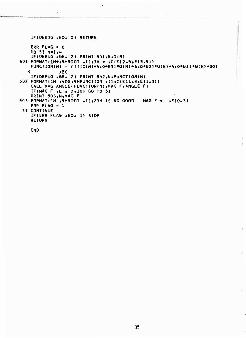
IF(DEBUG .EO. 0) RETURN

ERR FLAG « 0 DO 51 N«l«4 IF(DEBUG «GE. 2) PRINT 50l»NtO(N)

501 FORMAT(lH+t5HR00T »II.3H « ,C(E12.5.E13.5)) FUNCTION(N) ■ ((((O(N)+4.0*B3)*O(N)+6«0*B2)*O(N)+4.0«Bl)*O(N)+B0)

$ /BO IF(DE6UG «GE. 2) PRINT 502.N»FUNCTION(N)

502 FORMATdH .40X .9HFUNCTI0N ♦ 11 .C ( El 1.3 »Ell.S) ) CALL MAG ANGLE(FUNCTI0N(N).MAG F,ANGLE F) IF(MAG F .LT. 0.101 GO TO 51 PRINT 503»N»MAG F

503 FORMATdH ♦5HR00T .I1.23H IS NO GOOD MAG F « »E10.3) ERR FLAG « 1

51 CONTINUE IF(ERR FLAG .EO. 1) STOP RETURN

END

35

SUBROUTINE WAVEGUID

COMMOKVINPUT/THETA.IN OMIT(98) COMMON/FLG INPUT/FLG SKlPtRC PRINT.FLG OHIT(23) COMMON/WG INPUT/WGIN SKIP(7)»R POLY.WGIN OMIT(22)tEIGEN(30)f

S WGIN NO(10) COMPLEX THETA.EIGEN INTEGER RC PRINTfR POLY

R POLY

11

21

RC PRINT « 0 IF(R POLY «EO« 1) CALL GEN

INDEX « 1 THETA « EIGEN(INDEX) CALL ITERATE CALL COMP PROC EIGEN RL « El GEN (INDEXED IF(EIGEN RL .EQ. 0*0) 60 TO INDEX « INDEX+1 GO TO 11

RC PRINT « 1 RETURN

21

END

36

I SUBROUTINE ITERATE

COMMON/INPUT/THETA,IN OMIT(98) COMMON/WG INPUT/TYPE ITERtMAX DELTA.WGIN SKIP(88)»THETA INC»

f WGIN OMIT(2)»DTHETAtWGIN NO(5) COMMON/R/R SKIP(18).R11»R22»R 0MIT(4) COMMON/F/FfDFDTHETA,R BAR11.R BAR22 COMPLEX THETAfFO»F,DFDTHETA.DELTHETA»I.Rll.R22»R BAR11.R P>AR22t

$ EIGENtDTHETA REAL MAX DELTA,LUB REAL.LUB IMAG INTEGER TYPE ITER»RC PRINT,R POLY»FIRST»FIXED INC DATA(MAX ITER»2C)f(LUB REAL»0.05)»(LUB IMAG=0«005) DATA(I«(0.0,1.0) )

■

PRINT 101,TYPE ITER 101 F0RMAT(1H1,14HITERATI0N TYPE ,13)

PRINT 102,MAX DELTA 102 FORMATdH ,12HMAX DELTA = ,F5,2)

FIRST = 1 NR ITER » 0 ,

11 THETA = THETA-DTHETA CALL COMPUTE F FO = F THETA = THETA+DTHETA CALL COMPUTE F DFDTHETA « (F-FO)/DTHETA DELTHETA = -F/DFDTHETA FIXED INC - 1 GO TO 20

15 FO = F CALL COMPUTE F DFDTHETA « {F-FO)/DELTHETA DELTHETA « -F/DFDTHETA FIXED INC » 0

20 IF(FIRST .EQ. 0) GO TO 21 CALL PRINT RS $ CALL PRT THETA S FIRST « 0

21 DEL REAL « DELTHETA $ ABS REAL « ABSF(DEL READ IF(ABS REAL -GT. THETA INC) DELTHETA « DELTHETA#THETA INC/ABS REAL DEL IMAG = -I«DELTHETA $ ABS IMAG » ABSF(DEL IMAG) IF(ABS IMAG .GT. THETA INC) DELTHETA = DELTHETA»THETA INC/ABS IMAG THETA » THETA+DELTHETA CALL PRT THETA NR ITER = NR ITER+1 IF(NR ITER .GT. MAX ITER) GO TO 30 DEL REAL = DELTHETA $ DEL IMAG « -I#OELTHETA ABS REAL ' ABSF(DEL REAL) $ ABS IMAG = ABSF(DEL IMAG) IF(ABS REAL .LE. LUB REAL .AND. ABS IMAG .LE. LUB IMAG) GO TO 30 IF(ABS REAL .LE. MAX DELTA .AND. ABS IMAG .LE. MAX DELTA) 15»11

30 IF(FIXED INC .EO. 1) GO TO 31 THETA » THETA-DTHETA CALL COMPUTE F FO « F THETA = T HE TA-t-D THETA

37

CALL COMPUTE F DFDTHETA » (F-FO)/DTHETA

31 IF(TYPE ITER .EQ. 1) DFDTHETA « (R BAR22»R22-1.0)»DFDTHETA IF(TYPE ITER .EO. 2) DFDTHETA « (R BARI1»R11-1.0)»DFDTHETA

CALL PRINT RS PRINT SOltNR ITER

501 FORMAT(lH0t23HITERATIONS PERFORMED » .12) PRINT 502»DELTHETA

502 FORMATdHO.UHDELTHETA • .C(F11 .TtFll.T)) PRINT 503»F

503 FORMAT(1H0.13HF FUNCTION « tC(F13.5•F13.5)) RETURN

END

38

- .

SUBROLTINE COMPUTE F

C0MM0N/W6 INPUT/TYPE ITER.W6IN SKIP(6)*R POLYtWGlN OMIT(92) COMMON/R/R SKIP(18)»RlltR22»R!2.R21 COMMON/F/F.F SKIP(2)»R BARll.R BAR22 COMPLEX Rll»R22»R12»R21.FtR BARll.R BAR22 INTEGER TYPE iTERfR POLY

CALL R BARS

IF(R POLY .EO. 0) CALL INTEG IF(R POLY .EQ« 1) CALL USE POLY

IF(TYPE ITER .EO. 0) F ■ (R BAR11»R11-1,0)♦(R BAR22»R22-1.0) $ -R BAR11»R BAR22»R12*R21 IF(TYPE ITER .EO. 1) F « R BAR11»R11-1.0 IF(TYPE ITER .EQ. 2) F ■ R BAR22»R22-1.0 RETURN

END 1

39

SUBROUTINE R BARS

D»CAP OtCAP

COMMON/INPUT/THETA.FREQ KHZ»IN SKIP(3)tALPHA.HtD.IN 0MIT(91) COMMON/WG INPUT/WG SKIP(2)»EPSlLONtEPSILON O.SIGMA.WG OMIT(95) COMMON/F/F SICIP(4)fR BARll.R BAR22 COMMON/RB CP/S H FACTOR COMPLEX THETAtS H FACTOR.I.NG SO»C»S»SO ROOT.RATIO

PD.OD.H1 O.H2 D.HI PRIME O.H2 PRIME PO.OO.H1 O.H2 O.HI PRIME 0.H2 PRIME O.CAP A1ST.A2ND.A1.A2.A3.A4.R BAR11.R BAR22. C POWER.Z1.22.C TEMP. CPLX SQRT.CPLX EXPF.CPLX SINF.CPLX COSF

REAL K.LOG K OVR A.K OVER A OT.K OVER A TT.ND SO.NG DATA(PI»3,141592653) DATA(VEL LIGHT=2«997928E05) DATA(I=(0.0.1.0)) DATA(DEG TO RAD»0.01745329252) DATA(TEST TH IM»10.0)

RT. O.CAP HI

HI

SO

H2 H2

D. 0.

OMEGA « 2«0*PI»FREO XHZ»1000.0 K « 0ME6A/VEL LIGHT NG SO » (EPSILON-I#SIGMA/OMEGA)/EPSILON

C » CPLX C0SF(THETA»0E6 TO RAD) S » CPLX SINF(THETA»DEG TO RAD)

LOG K OVR A K OVER A OT K OVER A TT A OVER K OT A OVER K TT

LOGF(K/ALPHA) EXPFCLOG K OVR A/3.0) K OVER A OT»»2 1.0/K OVER A OT A OVER K OT*»2

ND SO » 1.0-ALPHA#(H-D) NO SO » 1.0-ALPHA»H SO ROOT » -CPLX SORT(NG SO-S»»2) RATIO RT » NO SO/NG SO«SO ROOT

PD « K OVER A TT»(1.0-ALPHA#(H-D)-S»»2) PO • K OVER A TT»(1.0-ALPHA»H-S»»2) 0 TERM ■ K OVER A TT»(ALPHA/X)»»2/4.0 00 • PD-0 TERM 00 • PO-0 TERM

THETA IM ■ -I»THETA IF(-THETA IM «GT. TEST TH IM .OR* D .EG. 0*0) GO TO 50 CALL MD HANKEL(0D.H1 D.H2 D.HI PRIME D.H2 PRIME D) CALL MD HANXELCOO.Hl 0.H2 O.HI PRIME 0.H2 PRIME 0)

CAP HI D » HI PRIME D+A OVER K TT#H1 D/2.0 CAP HI 0 ■ HI PRIME 0** OVER K TT»H1 0/2.0 CAP H2 D ■ H2 PRIME D-»-A OVER K TT»H2 D/2.0 CAP H2 0 ■ H2 PRIME 0*A OVER K TT#H2 0/2.0

A1ST » CAP H2 0-I»RATIO RT#K OVER A 0T»H2 0 A2ND « CAP HI 0-I«RATIO RT#K OVER A 0T»H1 0 Al « C»ND S0»(-H1 D*A1ST+H2 D»A2N0) S H FACTOR « (-A1ST#H1 0-t'A2ND»H2 0)/C-AlST«Hl D*A2ND»H2 D)

1*0

A1ST « -I«A OVER K OT»CAP H2 0-RATIO RT»H2 0 A2NO » -I*A OVER K OT»CAP HI 0-RATIO RT»H1 0 A2 = -CAP Hl D»A1ST+CAP H2 D*A2ND R BAR11 » (A1-A2)/(AH-A2)

CALL MO HANKEL(PD*H1 D*H2 D.HI PRIME D»H2 CALL MD HANKEL(POfHl O.H2 OtHl PRIME 0.H2

PRIME PRIME

D) 0)

A1ST « I »A OVER K 0T»H2 PRIME 0-fSO R00T»H2 0 A2ND = I*A OVER K 0T#H1 PRIME 0+SO R00T»H1 0 A3 = -HI PRIME D»A1ST*H2 PRIME D»A2ND A1ST « H2 PRIME 0-I»K OVER A 0T»S0 R00T»H2 0 A2ND « HI PRIME 0-I»K OVER A 0T»S0 R00T»H1 0 A4 « C»(-H1 D»A1ST+H2 D»A2ND) R BAR22 = (A3*A4)/(A4-A3) RETURN

C FLAT EARTH 50 C POWER »

R BAR11 « R BAR22 - Zl « C-^SQ Z2 = -C^SQ

CPLX EXPF(-2«0»I»K»D»C) (NG S0*C-S0 R00T)/(NG SO^C+SO R00T)»C POWER (C-SQ ROOT)/(C+SO ROOT)»C POWER ROOT/NG SO ROOT/NG SO

C POWER « CPLX EXPF(I»<»D»C) C TEMP « (Z1-Z2)/(Z1»C P0WER-Z2/C POWER) S H FACTOR » C TEMP»»2 RETURN

END

'♦1

SUBROUTINE COMP PROC

COMMON/1 NPUT/THETA,FREO ICHZ»IN SK IP( 3 ) »ALPHA,HtD» IN OMlT(91) COMMON/WG INPUT/WGIN SKIP(3)»EPSILON O.WGIN OMIT(2)t

$ REEL HT»W6IN NO(93) COMMON/F/F SKIP(2).DFDTHETA,R BAR11.R BAR22 COMMON/R/R SKIP(18)»R11.R22.R12»R21 COMMON/RB CP/S H FACTOR COMPLEX I.S.SORT S.E I PI OV ^.STORE l»STORE 2t

S S H FACTOR.SCRIPT H, S DFDTHETA»THETA.CPLX SQRTtCPLX SINFtS THETA P»C THETA S RllfR22.R12»R21»R BARll.R BAR22« S EXTRA,WAITS EF,DENOM»POLAR

REAL KtLOGElOtlMAG DATA(I«(0.0«1.0)) DATA(DEG TO RAD=0,01745329252)•(RAO TO DEG»57#29577951) DATACVEL LIGHT»2.997928E05) DATA(PI«3.1<»1592653) DATA(E I PI OV 4«(0.7071067812,0.7071067812)) DATA(LOGE10»2,302585093)

K ■ 2.0»PI»FRE0 ICHZ»1000.0/VEL LIGHT CAP IC » 1.0/<1.0-ALPHA»H/2.0) S « CPLX SINF(THETA»DEG TO RAD) S THETA P « CAP K»S STP REAL « S THETA P STP IMA6 » -I»S THETA P PHASE VEL « VEL LIGHT/STP REAL V OVER C ■ PHASE VEL/VEL LIGHT ATTEN « -8.6858896«K»STP IMAG»1000.0

SCRIPT H • EXPF(-ALPHA»D/2.0)»S H FACTOR SORT S « -CPLX SORT(S) STORE 1 « K»K»SORTF(K)»S»SQRT S»E I PI OV 4

$ /(2.0»EPSIL0N 0»S0RTF(2.0»PI)) STORE 2 « (1.0*R BAR11)»»2»(1.0-R BAR22»R22)#SCRIPT H»»2

S /(DFDTHETA/DEG TO RAD»R BARU) EXTRA ■ STORE 2»S WAITS EF « -HMC»REFL HT/2.0»EXTRA

CALL MAG ANGLE(EXTRA,EXTRA MAG,EXTRA ANG) EXTRA ANG « EXTRA ANG«DEG TO RAD CALL MAG ANGLE(WAITS EF,WAITS MAG,WAITS ANG) WAITS ANG * WAITS ANG»DEG TO RAD WAIT EF DB « 20.0»LOGF(WAITS MAG)/LOGE10

DENOM > R BAR11»R11-1.0 REAL - DENOM I MAG * -I«DENOM IF(REAL .EQ. 0.0 .AND. IMAG .EO. 0.0) DENOM > l.OE-150 POLAR « -R 8AR11»R12/DEN0M CALL MAG ANGLE(POLAR,POLAR MAG,POLAR ANG)

C THETA P « CPLX SORTd.O-S THETA P»»2) CTP REAL - C THETA P COS « SORTF{CTP REAL#»2-STP IMAG»«2) THETA P RL « ACOSF(COS)»RAD TO DEG

1*2

. r

THETA P IM » LOGFnCTP REAL+STP I MAG)/COS) »RAD TO DEG

PRINT 100 100 FORMATdHO»////)

PRINT 101»PHASE VEL 101 FORMATdH »2X»17HPHASE VELOCITY ■ »ElZ.StllH KM PER SEC)

PRINT 102»V OVER C 102 FORMATdH »2X»2AHPHASE VELOCITY OVER C = ,F9.5)

PRINT 103»ATTEN 103 FORMAT(1HO»2X»I4HATTENUATION = »E12,5»3H DB)

PRINT 104.EXTRA MAG 10A FORMATdH0»2X»12HEXTRA MAG « .E12.5)

PRINT 105»EXTRA ANG 105 FORMATdH »2X»14HEXTRA ANGLE = .F10.5.AH RAO)

PRINT 112.WAITS ANG 112 FORMATdH0.2X»35HPHASE OF WAITS EXCITATION FACTOR » »F10,5»4H RAD)

PRINT 113,WAIT EF DB 113 FORMATdH ,2X»32HWAITS EXCITATION FACTOR IN DB = »E12.5»3H DB)

PRINT 116.POLAR MAG 116 FORMATdH0»2X.19HPOLARIZATI0N MAG = »E12.5)

PRINT 117.POLAR ANG 117 FORMATdH .2X.21HP0LARIZATI0N ANGLE = .F10.5.4H DEG)

PRINT 118.THETA P RL.THETA P IM 118 FORMATdH0.2X.14HTHETA PRIME = .2F8.3.4H DEG)

PRINT 119 119 FORMATdHl)

RETURN

END

^3

SUBROUTINE WG OUTPUT

COMMON/INPUT/THETA.THETA IMG,IN OMIT{98) COMMON/R/R SKIP(18).R(4) COMMON/F/F.DFDTHETA,R BAR(2) COMPLEX R BARtRtALL RS,I•F.DFOTHETA REAL IMAG PART.MAG DATA(I = (0.0,Uu) ) DIMENSION ALL RS(8)tMAG(8)«ANGLE(8)tREAL PART(8)tIMAG PART(8)

ENTRY PRINT RS DO 11 J=1.2

11 ALL RS(J) = R RAR(J) DO 12 J«1.A

12 ALI RSCJ+2) » R(J) ALL RSCn « R BAR(1)»R(1) ALL RS<8) » R BAR{2)*R(2)

DO 13 Jal*8 CALL MAG ANGLE(ALL RS(J).MAG(J),ANGLE(J)) REAL PART(J) » ALL RS(J)

13 IMAG PART(J) ■ -I»ALL RS(J)

PRINT 200 200 FORMAT(1H0.8X»5HTHETA«5X,9H11R11 BARf6X,7HlRl BARt8X.5H11R11,

$ 10X»3HlR1.9Xt4HlRll,9X»AHnRl,2X.llHRll BAR»R11» $ 4X»9HR1 BAR*R1/)

PRINT 201»THETA,(REAL PART(J).J«l»8 ) 201 FORMATdH t4HREAL.F9.3tlX»8E13.5)

PRINT 202.THETA IMG,(IMAG PART(J)•J«l,8) 202 FORMATdH ,4HIMAG,F9.3,lX »8E13 .5 )

PRINT 203,(MAG(J),J=1,8) 203 FORMATdH ,3HMAG, 11X,8F13.5 )

PKTNT 204,(ANGLE(J),J=1,8) 204 FORMATdH »SHANGLE, 9X,8F13.5)

RETURN

ENTRY PRT THETA CALL HAG ANGLE(F,F MAG,F ANGLE) CALL MAG ANGLE(DFDTHETAtDFDT MAG.OFDT ANGL) PRINT 500,THETA,THETA IMG.F MAG,DFDT MAG

500 FORMATdH0,8HTHETA » ,2F10,3,10X,8HF MAG = ,E10,3,5X, $ 15HDFDTHETA MAG « ,E10.3)

RETURN

END

kh

SUBROUTINE MD HANKEL(Z»Hl ,H2,H1 PRIME»H2 PRIME)

COMPLEX 2fItHl.H2.Hl PRIME,H2 PRIME, »ZCUBED.Z POWER.TERM1.TERM2. $ TERM3 »TERM4.TERMS»TERM6.SUMl»SUM2,SUM3,SUM4,SUM5tSUM6» $ SUM7.SUM8»FfG»F PRIME»G PRIME.ONE Rl r Z.CPLX SORT. % I FOURTH•SORT 2 CUB. ,EXP1.EXP2.EXP3.EXP4.EXP5,. S CPLX EXPFtBETA.RT Z.6M2i ♦r1PMFP, I POWERtM I POWERt $ 2 M3HALVS.2 MSHAFf, M

DIMENSION A(23) »B(23)»C(23)»D(23)»CAP(14)

DATA(A« 0.9304 3671 693 . 31.0145 5723 097. 206.7637 1487 316. S 574,3436 5242 545, . 870.2176 5519 008, > 828.7787 1922 864, S 541.6654 3740 434, , 257.9454 4638 302i 93.4584 9506 631. S 26.6263 5187 074, i 6.1210 0043 0056, 1.1592 8038 4480. S 0.184U 1275 9441, » 0.0248 3303 0964, 0.0028 8420 8010. S 0.0002 9133 4142 , 0.0000 2582 7495, 0.0000 0202 5686. S 0.0000 0014 1557 » 0.0000 0000 8870, . 0.0000 0000 0501. S 0.0000 0000 0026, » o.oooc 0000 0001

DATA(B= 0.6782 9872 514, » 11.3049 7875 240, . 53.8332 3215 431. S 119.6294 0478 735, . 153.3710 3177 865, 127.8091 9314 888. S 74.7422 1821 572 > 32.3559 3862 152, 10.7853 1287 384. S 2.8532 5737 403 • 0.6136 0373 6351, » 0.1093 7678 98. S 0.0164 2293 9955, » 0.0O21 0550 5122, . 0.0002 3316 7788. S 0.0000 2252 8289, . 0.0000 0191 5671, . 0.0000 0014 4470. S 0.0000 0000 9729, » 0.0000 Ü&0C 0589, 0.0000 0000 0032. S 0.0000 0000 0002 » O.OOCO 0000 0000

DATA(C= 0.4652 1835 846, > 6.2029 1144 619i 25.8454 6435 915. S 52.2130 5931 140, . 62.1584 0394 215. 48.7516 8936 639. $ 27.0842 7187 022, . 11.2150 1940 796i 3.5945 5750 255. S 0.9181 5006 451, » 0,1912 8126 3439, 0.0331 2229 6699. S 0.0048 4244 1038, . 0.0C06 0568 3682, O.OOCO 6555 0182. S 0.0000 0619 8599, . 0.0000 0051 6550, . 0.0000 0003 8220. S 0.0000 COOO 2528, . 0.0000 0000 0150, . 0.0000 0000 0008. S 0.0000 0000 0000, > 0.0000 0000 0000

DATA(D» 0.6782 9872 514, » 45.2199 1500 962, . 376.8326 2508 015. $ 1196.2940 4787 350, .1993.8234 1312 250, »2044.9470 9038 206. S 1420.1021 4609 865, . 711,8306 4967 361, . 269.6328 2184 603. S 79.8912 0647 290 . 19,0217 1582 6880, » 3.7188 1052 3339. $ 0.6076 4877 8323, ► 0,0842 2020 4896 » 0.0100 2621 4869. $ 0.0010 3630 1278, . 0.0000 9386 7869 » 0.0000 0751 2435. S 0.0000 0053 5074, . O.OOCO 0003 4135, » 0.0000 0000 1962. S 0.0000 0000 0102 . 0,0000 0000 0005

DATA(CAP»0.1041 6666 6666 6666 7»0'.0835 5034 " T222 2222 2. r

S 0.1282 2657 4556 3271 6.0.2918 4902 ( >464 1404 6. S 0.8dl6 2726 7443 7576 5.3.3214 0828 ] L862 768. S 14.9957 6298 686i ? 6.78.9230 1301 158- r.474.4515 3886 8. S 3207.4900 91.2 4( )86.5496.19 8923.12.] 179 1902.0 » S 1748 4377.0)

DATA{PI»3.1415 92653 58979) DATA(Is(0.0.1.0)) DATA(ALPHA«0.853 667 218 838 951)

U5

r

CALL MAG ANGLE(Z*ZMAGfPHI)

Z POWER «1.0 Z CUBED » Z»»3

IFCZMAG .GT. 4.21 GO TO 50

IF(ZMAG .LT. 3.2) 21*22 21 N«12

GO TO 30

22 IF(ZMAG «LT. 4.1) 23*24 23 N»15

GO TO 30

24 N-23

30 SUM1 ■ 0.0 SUM2 « 0*0 SUM3 • 0.0 SUM4 «0.0

DO 31 M«1*N TERM1 « A(M)»Z POWER TERM2 « B(M)»Z POWER TERM3 « C(M)#Z POWER TERM4 « D(M)»Z POWER SUM1 « SUMH-TERM1 SUM2 ■ SUM2+TERM2 SUM3 « SUM3-»-TERM3 SUM4 « SUM4*TERM4 Z POWER ■ -Z CUBED/200,0»Z POWER

31 CONTINUE

F ■ SUM1 G ■ Z»5»UM2 GM2F » G-2«0»F F PRIME ■ -Z»»02«SUM3 G PRIME ■ SUM4 GPMFP ■ G PRIME-2.0»F PRIME RT THIRD « SQRTF{1.0/3.0)

HI « G*I»RT THIR0»GM2F HI PRIME » G PRIME-H^RT THIRD»GPMFP

H2 ■ 6-I»RT THIRD»GM2F H2 PRIME ■ G PRIME-I«RT THIRD»GPMFP

RETURN

50 SUM5 «1.0 SUM6 « 1.0 SUM? « 0.0 SUMO «0.0 Z REAL » Z Z IMAG « -I»Z I POWER « I

1*6

M I POWER » -I RT 2 » CPLX SORTCZ) IF(Z IMAG .LT, 0.0) RT Z » -RT Z ONf: RT Z « 1.0/RT Z Z FOURTH « CPLX SORT(RT 2) REAL Z 4TH » Z FOURTH IF(REAL Z 4TH «LT. 0,0) 2 FOURTH « -2 FOURTH BETA « ALPHA/2 FOURTH SORT 2 CUB « RT 2»»3 2 M3HALVS = 1.0/SORT 2 CUB 2 M3HAFS M « 2 M3HALVS EXP1 « CPLX EXPF(I»2.0/3,0»SORT 2 CUB) EXP2 « EXP1»CPLX EXPF(-I*5,0/12.0»PI) EXP3 « 1.0/EXP1»CPLX EXPF(I»5.0/12.0»PI) EXP4 » EXP1»CPLX EXPF(I*11.0/12.0»PI) EXP5 « 1.0/EXP1»CPLX EXPF(-I»11,0/12.0»PI)

00 51 M=l,14 TERMS ■ I P0WER»CAP{M)»2 M3HAFS M TERM6 • M I P0WER»CAP(M)*2 M3HAFS M SUMS « SUMS+TERMS SUM6 * SUM6-»-TERM6 EM • M SUM? ■ SUM7-M-1.5»EM«1#0/2)»TERM5 SUMS « SUM8-M-1.5»EM»1«0/2)»TERM6 2 M3HAFS M ■ 2 M3HAFS M»2 M3HALVS 1 POWER « I POWER»I M I POWER « M I POWER»(-I)

SI CONTINUE

IF(2 REAL .GE. 0.0 .OR. 2 IMAG «GE. 0*0) 61.62 61 HI « BETA»EXP2»SUW6

HI PRIME * BETA»EXP.»(SUM6»(-0»2S»1.0/2-M#RT 2)*SUM8) GO TO 70

62 HI • BETA»(EXP2»SUM6't-EXP5»SUM5) HI PRIME ■ BETA»<EXP2»(SUM6»(-0«25»l«0/2-M»RT 2)+SUM8)^EXP5«(SUMS

S ♦(-0«25»l«0/2-I»RT 2)'«-SUM7) )

70 IF(2 REAL «GE. 0.0 «OR* 2 IMAG .LT* 0.0) Vl»72 71 H2 « BETA»EXP3»SUMS

H2 PRIME « BETA»EXP3#(SUM5»(-0.25»1.0/2-I»RT 2)*SUM7) RETURN

72 H2 » BETA»(EXP3»SUMS4EXP4»SUM6) H2 PRIME » BETA»{EXP3»(SUMS»(-0.25»1.0/2-I»RT 2 )^SUM7)-»-EXP4»( SUM6

S »(-0.25»1.0/2*I*RT 2)*SUM8)) RETURN END

^7

SUBROUTINE R POLYNOM

COMMON/INPUT/THETA,IN OMIT(98) COMMON/WG INPUT/WGIN SKIP(8)»T LIST(11)»WGIN OMIT(70) COMMON/R/LOG R(4)»R SKIP(10)tR(4) COMMON/1 NIT R/ADJ FLAG COMPLEX THETA.LOG RtR.LOG R MTRXtT LIST.LAGR INTPtCPLX EXPF INTEGER DIMENSNtADJ FLAG.DEBUG DIMENSION LOG R MTRX(10t4)

ENTRY GEN R POLY PRINT 100

100 FORMAT!1H f/////»29HR MATRIX INTERPOLATION POINTS)

M - 1 11 THETA « T LIST(M)

CALL INTEG DO 12 N«1.4

12 LOG R MTRX(MfN) « LOG R(N) IF(T LIST(M*1) «EO. 0.0) GO TO 13 ADJ FLAG • 1 M ■ M+l S GO TO 11

13 DIMENSN ■ M ADJ FLAG « 0

PRINT 300 300 FORMAT*1H0«6X«6HT LIST*14X«5H11R11*17X*3H1R1•

S 17Xt4HlRll*19X*4HllRl) DO 31 M-l«DIMENSN

31 PRINT 301.T LIST(M).(L0G R MTRX(M«N)«N»l•*) 301 FORMATdH , 1X.C (F6.2 .F6.2) .M 2X.C(F10.4,F10.2 )) )

RETURN

ENTRY USE POLY

DO 91 N«l«4 LOG R(N) - LAGR INTP(T LISTtLOG R MTRX(1«N)»THETA.DIMENSN)

51 R(N) • CPLX EXPFaOG R(N)) RETURN

END

kS

FUNCTION LAGR INTP(X.YtXO.N)

COMPLEX X.Y.XG.LAGR INTP.SUMtPROD DIMENSION X(N)»Y(N)

SUM « 0*0 DO 12 J»ltN PROD * 1*0 DO 11 I«1«N IF(I .EO. J) GO TO 11 PROD ■ PROD»(XO-X(in/(X(J)-X( in

11 CONTINUE 12 SUM « SUM"fPROD»Y(J)

LAGR INTP « SUM

END

k9

SUBROUTINE INTEG C BUDOEN

COMMON/INPUT/IN SKIP(8)tDtREL PREC^TOP HTtIN OMIT<89» COMMON/FLG INPUT/DEBUGtRC PRINTtFLG OMIT(23) COMMON/R/LOG R(8)»DLOGRDHC8)»HTvDELHtR OMIT(8) COMMON/1/L.HT LIST(256)tOMlTl(256*3) REAL LOG R.LOG N LlSTtLOGR O.LOWEST HTtLOGElO INTEGER S FLAG»DEBUG»RC PRINT DIMENSION LOGR 0(8)*OLOGRDH 0(8)*

$ DEL LOGR 0(8).DEL LOGR 1(8)»DEL LOGR 2(8) DATA(DELHMIN=0.03125) DATA(LOGE 10 = 2.302585093)

FACTOR « EXPF(-REL PREC#LOGE10) EMAX « 3.0»FACTOR EMIN • 0.3»FACTOR L « 1 HT » TOP HT DELH « DELHMIN SAVE DELH • DELH CALL INIT COMP CALL S MATRIX CALL INITIAL R CALL R DER IV IF(RC PRINT «EO. 1 • OR. DEBUG • .GE. 1) PRINT 100

100 FORMAT(1H0*15X*21H R-MATRIX INTEGRATION ) IF(RC PRINT .EG. 1 •OR. DEBUG .GE. 1) CALL R COL HEAD IF(RC PRINT .EO. 1 .OR. DEBUG «GE« 1) CALL PRINT R

C RUNGE KUTTA 20 S FLAG ■ 0

IF(HT .EO. HT LISTa+D) L ■ L*l IF(HT-DELH .GE. HT LISTIL*!)) 60 TO 21 DELH - HT-HT LlST(L+l) S FLAG ■ 1

21 IF(HT-DELH .LT^ D) DELH ■ HT-D

DO 31 1*1*8 LOGR 0(1) ■ LOG R(I)

31 DLOGRDH 0(1) ■ DLOGRDH(I) C TRY AGAIN

33 DO 34 1=1,8 DEL LOGR 0(1) • -DLOGRDH 0(1)«DELH

34 LOG R(I) » LOGR 0(I)+0.5»0EL LOGR 0(1)

HT ■ HT-0.5»DELH CALL S MATRIX CALL R DER IV

DO 35 1-1*8 DEL LOGR 1(1) « -DLOGRDH(I)»DELH

35 LOG R(I) ■ LOGR 0(I)*0#5»DEL LOGR 1(1)

CALL R DER IV

50

ü

DO 36 I»l*8 DEL LOGR 2(1) « -DL06R0H(I)»DELH

36 LOG Rd) « LOGR 0(I)+OEL LOGR 2(1)

HT « HT-OELH-»-0.5»DELH CALL S MATRIX CALL R DER IV

ERROR «0*0 DO 37 I«1.8 DEL LOGR 4 « ((-DLOGRDM( I )*DELH-fDEL LOGR 0(I))/2.0

S +OEL LOGR KD-fDEL LOGR 2(in/3.0 LOG R(I) « LOGR 0(1)♦DEL LOGR 4 ERR - ABSFCDEL LOGR 2(I)-DEL LOGR 4) IF(ERROR «LT. ERR) ERROR • ERR

37 CONTINUE IF(ERROR .GT. EMAX «AND« DELH .GT. DELHMIN) 38*40

38 HT « HT^DELH DELH ■ OELH/2.0 IF(DELH .LT. DELHMIN) DELH « DELHMIN GO TO 33

40 CALL R DER IV IF(RC PRINT «EO. 1 «OR. DEBUG «GE* 1) CALL PRINT R IF(ERROR «LT. EMIN) DELH > 2.0«DELH IF(S FLAG .EQ. 1) DELH ■ SAVE DELH SAVE DELH « DELK IF(HT .GT. D) GO TO 20

IF(RC PRINT .EO. 1) CALL RATIO DIF RETURN

END

51

SUBROLTINE DER IV EOU

COMMON/lNPUT/THETA,FRE(J KHZ»AZ IMUTHtDIP ANGLEtMAG FIELD»ALPHA»H» S IN OMIT(92» COMMON/SP INPUT/NR SPEC.COEFF NUOl.EXP NU( 3 ) »CHARGEC 3 ) tM RATIO(3) COMMON/FLG INPUT/FLG SKIP(5).NEG ELECT»FLG 0MIT(19) COHMON/R/LOG Rll»LOG R22.LOG R12»LOG R21,

S OLNRllDHfOLNR22DH,DLNR12DH»OLNR210H( S HT.R SKlPtRlltR22*R12*R21 COHMON./M/Mll«M12»M13»M21*H22tM23*M31tM32»M33*CtStCSO COMMON/1/L.HT LIST(256)tLOG N LIST(256.3) COMPLEX I.THETA.K OVER 21t

S C.S.CSO.ONE OVER C«S OVER C. $ iLYtlMY.INY.U.USOtD. S Mll»M12*M13»M21*M22fM23*M31.M32*M33« S T11,T31»T42,T44» S T12 OVER C»T14 OVER CfT32 OVER C»T34 OVER C»CT4l» $ SllAfDllAvSllB*OnB»S12tD12*S21<021tS22<D22t S B11.B22»B12.B21.R12R21.C12.C21, S DERlVll«DERIV22fDERlV12tDERlV21« S Rll»R22.R12tR21tL0G RlltLOG R27»LOG R12*LOG R21» S OLNR110H,DLNR22DH,DLNR12DH»DLNR21DH, $ CPLX LOGFtCPLX EXPF.CPLX COSF.CPLX SINF REAL MAG FIELD.M RATIO.LOG NtLOG N LIST»

S LSOYSO*MSOYSO»NSOYSO«LMYSO«LNYSO»MNYSO DIMENSION X(5)tY(5).YSO(5J»Z(5).COLL FREO(5 ) .EN(5).

S ILY(5)»IMY(5),INY(5),LSQYSQ(5).MSOYSO(5).NSOYSO(5J» $ LMYSO(5)»LNYSO{5).MNYSO(5) DATA(PI»3*141992653) DATA(DEG TO RAD»0.01745329252) DATAJCOEFF Y-1.758796E11)»(COEFF X«3.182357E03) DATACVEL LIGHT«2.997928En5) DATA(I«(0*Otl«0))

ENTRY IN IT COMP OMEGA • 2*0*PI«FREQ KHZ»1000.0 K OVER 21 ■ (OMEGA/VEL LIGHT)/(2.0»I) SIN DIP « SINF(DIP ANGLE*DEG TO RAD) DIR CCS L ■ SIN DIP*COSF(AZIMUTH*DEG TO RAD) DIR COS M ■ SIN DIP*SINF(AZIMUTH«DEG TO RAD) DIR COS N ■ -COSF(DIP ANGLE»DEG TO RAO) C « CPLX COSF(THETA#DEG TO RAD) CSO • C»C S ■ CPLX SINF(THETA#DEG TO RAO) ONE OVER C « l.O/C S OVER C • S/C

DO 11 K«ltNR SPEC Y(K) ■ COEFF Y»CHARGE(>:)»MAG FIELD/(OMEGA»M RATIO(K)) YSO(K) ■ Y(K)»#2 ILYOC) • I»DIR COS L»YCK) IMYCK) • I»DIR COS M»Y(IC) INYCK) « I»DIR COS N»Y(K) LSOYSO(K) « DIR COS L»»2»YSO(K) MSOYSO(K) «DIR COS M»»2»YSO(K) NSOYSO(K) ■ DIR COS N#»2»YSO(K) LMYSO(K) ■ DIR COS L«DIR COS H»YSO(K)

52

LNVSOm « DI c»OIR COS N»YSO(K) 11 MNYSO(K) « DI; .o M»DIR COS N»YSO(K)

RETURN

ENTRY S MATRIX Mil ■ 0.0 S M12 - 0.0 S M13 « 0*0 M21 « 0.0 $ M22 = 0.0 f M23 * 0.0 M31 « 0.0 S M32 = 0.0 S M33 = 0.0

DO 24 K«1»NR SPEC LOG N » LOG N LIST(L+1 .K )"MHT-HT LIST(L-H))

S /(HT LIST(L)-HT LlSTfL-H)» $ «(LOG N LIST(L.K)-L0G N LIST(L+ltK)) EN(K) » EXPF(LOG N) X(IC» - COEFF X»(1.0E06#EN(Kn»CHARGE'K)»»2/(OMEGA**2«M RATIO(<)) IF(NE6 ELECT .EQ. 1) X(K) » -X(K) COLL FREO(K) « COEFF NU(K)*EXPF(EXP NU(K)»1000.0»HT) UK) » COLL FREO(K)/OMEGA IF(NEG ELECT .EO. 1) Z(K) « -Z(IC) U » 1.0-I»Z(K) USO ■ U»U D « -X(K)/(U*nJS0-YSQ(JOn Mil » Mll-KUSO-LSOYSO(K) )»D M12 « M12-».(-INY(K)»U-LMYSO(<) )»D M13 » M13-MIMY(K)*U-LNYSO(K) )*D M21 ■ M21-f(INY(K)»U-LMYSO(K) )«D M22 ■ M22'MUSO-MSOYSO(K) )»D M23 « M23-K-ILY(K)»U-MNYS0(K))«D M31 « M31-f(-IMY(K)»U-LNYSO(K) )»D M32 « M32-MILY(IO»U-MNYSO(K) )»D

24 M33 » M33-KUSO-NSOYSO(K) )»D

CURV TERM • ALPHA»(H-HT) Mil » Mll-CURV TERM M22 « M22-CURV TERM M33 ■ M33-CURV TERM

D * 1.0/(1.0+M33) Til ■ -S»M31»D T12 OVER C ■ S OVER C*M32»D T14 OVER C » (C+M33»ONE OVER C)»D T31 ■ M23#M31#D-M21 T32 OVER C » C"MM22-M23»M32»D)»0NE OVER C T34 OVER C « S OVER C»M23*D CT41 » (1.0*M11-M13»M31»D)«C T42 ■ M32»M13»D-M12 J*U m -S»M13»D

S11A » T11+T44 DUA « T11-T44 SUB « T14 OVER C+CT41 DUB « T14 OVER C-CT41 S12 ■ T12 OVER C'«-T42 D12 » T12 OVER C-T42 521 ■ T34 OVER C+T31 D21 « T34 OVER C-T31 522 » C*T32 OVER C D22 « C-T32 OVER C

53

RETURN

ENTRY R DERIV Rll = CPLX EXPF(LOG RU) R22 « CPLX EXPF(LOG R22) R12 = CPLX EXPFCLOG R12) R21 « CPLX EXPF(LOG R21)

RL LOG R12 = LOG R12 IF(RL LOG R12 .LT, -11.0) R12 • 0.0 RL LOG R21 « LOG R21 IF(RL LOG R21 .LT. -11.0) R21 ■ 0.0

Bll z R1HMD11A- -DUB) B22 ■ R22«022 B12 ■ R12»D21 B21 s R21»S12 R12R21 « R12»R21 C12 « R12»S21 C21 « R21»012

DERIV11 « Bll-».B12-»-B21-SllB-SllB'»-(R12R21»D22*C12+C21-DllA-DllB)/Rll DERIV22 ■ B12-»-B21+B22-S22-S22-f(R12R21»(DllA-DllB)-fB12+B21-»'D22)/R22 DER IVI2 ■ Bll-»-B12+B22+SllA-SllB-S224-(Rll«Sl24012)»(R22*l«0)/Rl2 DERIV21 ■ Bll4B2H-B22-SllA-SllB-S22-»-(Rll»D21+S21)»(R22+1.0)/R21

DLNR11DH « K OVER 2I»DERIV11 DLNR22DH > K OVER 2I«DERIV22 CLNR12DH » K OVER 2I»DERIV12 DLNR21DH « K OVER 2I*DERIV21 RETURN

END

3k

SUBROUTINE INITIAL R

COMMON/INPUT/IN SICIP(5)»MAG FIELOtIN 0MIT(94) COMMON/FLG INPUT/0EBU6»FL6 OMIT(24) COMMON/R/LOG RUtLOG R22*LOG R12.LOG R21«R SKIP(IO)»

S Rll,R22tR12.R21 COMMON/INIT R/ADJ FLAG COMMON/M/MlltM12tMl3»M21.M22»M23tM31.M32»M33fCtS.CS0 COMPLEX Mll«M12fM13»M21»M22*M23*M31*M32»M33tCfStCSQ«

B3tB2tBl*B0«O*C TEMP« Dl1»013«D31»033«DELTA*P«T«01.02»PI«P2»T1«T2* R11*R22*R12»R21« LOG RlltLOG R22»L0G R12»L0G R21» FN S0«F ROOT» CPLX SQRT»CPLX LOGF»CONJ

REAL MAG FIELD,MAG 0 INTEGER DEBUGtADJ FLAG DIMENSION DIFF(4),0(4)tP(2)»T(2) DIMENSION PHASE R(8)»PREV PHA5(8) DATA(PI«3.141592653) DATACADJ FLAG«0) EQUIVALENCE(0(1).01)»(0(2)»02).(P(1).PI)♦»P(2>♦P2)♦

S (T(1).T1).(T(2).T2) EQUIVALENCE(LOG R11.PHASE R)

IF(MAG FIELD .EO. 0.0) GO TO 50

B3 « S»(M13-»-M31)/(4.0»(l.O-fM33)) B2 « (-(CSQ-t-M33)»(1.0*Mll)-»-M13»M31-(1.0-»-M33)»(CSO+M22)^M23»M32)

$ /(6.0»(1.04-M33)) Bl » S»<M12»M23-fM21*M32-(CSO*M?2)»(M13+M31))/(4.0»(1.0*M33)) BO «( 11.0*Mll)»(CSO*M22)»(CSQ+M33)-»'M12»M23»M31-«-M13»M21*M32

$ -M13*(CSO+M22)»M31-(1.0+M11)»M23»M32-M12»M21»(CSQ4-M33) ) $ /(1.0+M33)

CALL CJARTIC(B3.62.61.80.0.DEBUG)

DO 12 N«l»4 CALL MAG ANGLE(0(N)«MAG Q.ANGLE 0) IF(ANGLE 0 .LT« 135.0) ANGLE Q « ANGLE 0+360.0

12 DIFF(N) ■ AeSF(ANGLE Q-315.0)

DO 15 M«2«4 DO 15 N»M*4 IF(DIFF(N) .GT. DIFF(M-l)) GO TO 15 TEMP ■ DIFF(N) S DIFF(N) « DIFF(M-l) $ DIFF(M-1| « TEMP C TEMP ■ 0(N) f 0(N) « O(M-l) $ Q(M-1) « C TEMP

15 CONTINUE

DO 21 N-1.2 Dll « l«0-fMll-0<N)»»2 D13 ■ M13*S»Q(N) D31 » M31-»-S»Q(N) D33 ■ 1#0*M33-S»«2

DELTA « D11»D33-D13»D31 P(N) « (-M12»D33-»-D13#M32)/DELTA

55

T(N) = Q(N)»P(N)-S*{-D11»M32*M1?*D31)/DELTA POYNTING » CONJ(P(N))#(Q{N)»P(N)-S»T{N))+Q{N) IF(POYNTING .LT. 0.0) PRINT 201»Q(N)»POYNTING

201 FORMAT(1HO»8HFOR Q = ♦C(E11,3.E11.3)»UHPOYNTING » .Ell.3) 21 CONTINUE

DELTA « (Tl»C+Pl)»(C+02)-(T2»C+P2)»(C+01) Rll = » (Tl»OPl)»(O02)-(T2»C-P2)»(C+Qin/DELTA R22 = ((Tl»C+Pl)«(C-02)-{T2»C4-P2)»(C-Ql))/0ELTA R12 *-2.0»CMTl»P2-T2»Pl)/0ELTA R21 =-?.0»C»(01-Q2)/DELTA

22 LOG Rll ■ CPLX LOGF(Rll) LOG R22 ■ CPLX LOGF(R22) LOG R12 s CPLX LOGF(R12) LOG R21 s CPLX LOGF(R21)

IF(ADJ FLAG »EO. 0) GO TO 36 DO 35 N=2»8»?

33 IF(PHASE R(N)-PREV PHAS(N) .LE, PI) GO TO 34 PHASE R<N) = PHASE R(N)-2.0*PI $ GO TO 33

34 IF(PREV PHAS(N)-PHASE RtN) .LE. PI) GO TO 35 PHASE R(N) = PHASE R(N)*2.0»PI $ GO TO 34

35 CONTINUE 36 DO 37 N»2»8,2 37 PREV PHAS(N) « PHASE R(N)

RETURN

RS BY FRESNEL 50 FN SO = 1,0+Mll

F ROOT « -CPLX SORT(FN SO-S»«?) Rll « (FN SO»C-F ROOT)/(FN SO#C-«-F ROOT) R22 « (C-F ROOT)/(C-»-F ROOT) R12 « 0,0 S R21 « 0.0 GO TO 22

END

56

w*

SUBROUTINE R OUTPUT

COMMON/R/LOG RlltRll AN6LF»LOG R22.R22 ANGLE* S LOG R12»R12 ANGLE»LOG R21.R21 ANGLE« $ R SKIP(8)»HT»R 0MIT{9) REAL LOG RlltLOG R22.LOG R12*LOG R21 DATA(RAO TO DEG»57.29577951)

ENTRY R COL HEAD PRINT 100

100 FORMAT(lHO»8Xt2HHT.10Xt5HllRllf17X.3HlRlf16X»4H1R11,16X.4H11R1) RETURN

ENTRY PRINT R Rll MAG « EXPFaOG RID R22 MAG « EXPF(LOG R22) R12 MAG « EXPF(LOG R12) R21 MAG « EXPFCLOG R21) DEG11 » Rll ANGLE»RAD TO DEG OEG22 • R22 ANGLE*RAO TO DEG DEG12 » R12 ANGLE»RAD TO DEG DEG21 = R21 ANGLE»RAO TO DEG

PRINT 20n.HT,Rll MAG.DEGll,R22 MAG.DEG 22fR12 MAG.DEG12» f R21 MAG»DEG21

200 FORMATdH »Fin^^ f F10.4tF10,2 ) ) RETURN

ENTRY RATIO DIF RATIO « R12 MAG/R22 MAG DIFF « DEG12-DEG22

PRINT 301fRATIO 301 FORMAT(lH0tl9HlRll MAG/1R1 MAG « tE12.5)

PRINT 3C2«OIFF 302 FORMATdH .23H1R11 ANGLE-1R1 ANGLE « ^11.5)

PRINT 303 303 FORMAT(lHl)

RETURN

END

57

RSFSRENCSS

1. Smith, R., "Program for the full-wave calculation of reflection In an arbitrary.Ionosphere (U)," DASA Report l6l5, 1965.

2. Gossard, iS.E., et al, "A computer program for vlf mode constants In an earth-ionosphere waveguide of arbitrary electron density distri- bution," MIPR DASA No. 550-^, I966.

3. Gossard, E.E., Y. Gough, V. Noonkester, R, Pappert, I. Rothmuller, R. Smith, and P. Winterbauer, "A computer program for vlf mode con- stants in an earth-ionosphere waveguide of arbitrary electron density distribution," Navy Electronics Laboratory Interim Report No. 671 for DASA, September 1966.

U. McKinley, R.R., "A rigorous waveguide program for a cyllnderical waveguide," NEL Tech Memo I315, Oct. I967.

5. Pappert, R.A, and C.H. Sheddy, "An accelerated waveguide program," Navy Electronics Laboratory Tech Memo IOUO, Jan 1967.

6, Pappert, R.A., "On the problem of horizontal dipole excitation of the earth-ionosphere waveguide," NEL Interim Report 681f for DASA, April I968.

7* Sheddy, C.H., Y. Gough, and R.A. Pappert, "An improved computer program for vlf mode constants In an earth-ionosphere waveguide of arbitrary electron density distribution," NEL Interim Report No. 682 for DASA, February I96Ö.

8. Budden, K.G., "The numerical solution of differential equations governing reflection of long radio waves from the Ionosphere," Proc. Roy. Soc. (London), A &1, 516 (1955).

9. Sheddy, C.H., "A general analytic solution for reflection fron a sharply bounded anisotropic ionosphere," to be published In Radio Science, August 1968.

10. Budden, G.G., "The Influence of the earth's magnetic field on radio propagation by waveguide modes," Proc. Ray. Soc. (London) Ser. A265, »0. 1323, 538-553i (1962).

11« Pappert, R.A., E.E. Gossard, I. Rothmuller, "A numerical investigation of classical approximations used In vlf propagation," Radio Science, 2 »o. k, 387-400.

12. Staff of the Computation Laboratory at Cambridge, Mass., "Tables of the modified Hankel functions of order one-third and of their derivatives," (Harvard Univ. Press, Cambridge, Mass) (1945)«

13, Wait, J.R., "Electromagnetic waves in stratified media," p. 221 (Per- gamon Press, New York, N.Y.), (1962).

Ik, Pappert, R.A., "A numerical sutdy of vlf mode structure and polarization below an anisotropic ionosphere," Radio Science, 3, No. 3, 219-233, 1968.

58

INITIAL DISTRIBUTION LIST

Director Defense Atomic Support Agency Attn: RAAB Washington, D. C. 20305

Director (2) Defense Atomic Support Agency Attn: Technical Library Washington, D. C 20305

Commander Test Command Defense Atomic Support Agency Sandla Base, New Mexico 87115

Director of Defense Research & Engineering

Attn: Atomic Programs Washington, D. C. 20301

Commander Joint Task Force EIGHT Sandla Base Attn: Technical Library Albuquerque, N. Hex. 87115

Atomic Energy Commission Albuquerque Operations Office Attn: Dr. D. W. Sherwood P.O. Box 5400 Albuquerque, N. Hex. 87100

U.S. Atomic Energy Commission Special Asst. for Disarmament Attn: Dr. Allen M. Labowltz Washington, D. C 205^5

Director of Military Application U.S. Atomic Energy Commission Attn: Mr. Donald Gale Washington, D. C 205^5

Director Defense Intelligence Agency Attn: Hq-Tr; Mr. J. H. Stewart Washington, D. C 20301

Director Nuclear Test Detection Advanced Research Projects Agency Washington, D. C. 20301

Director (2) Advanced Research Projects Agency Attn: F. A. Koether

Dr. Paul Tamarkln Washington, D. C. 20301

Director Weapons Systems Evaluation Group Attn: Library Washington, D. C. 20301

Defense Communications agency (2) Attn: Mr. Probst Code 513

Dep Director for NMCSTS 8th & So. Courthouse Road Arlington, Va. 22204

ITSA/ESSA (6) Attn: A. Glenn Jean

W. Taylor J. R. Johler R. Knecht D. D. Cromble L. A. Berry

Boulder, Colorado 80302

National Bureau of Standards (2) U.S. Department of Comerce Attn: Mr. Arthur Ernst

Mr. Raymond T. Moore Washington, D. C. 20234

Defense Documentation Center (20) Cameron Station Alexandria, Va. 22314

Chairman Joint Chiefs of Staff Attn: J-6 Washington, D. C. 20301

Chief of Research & Development Department of the Army Attn: LTC0L Dayton Washington, D. C 20310

Director Army Ballistic Research Laboratories Attn: Technical Library Aberdeen Proving Grounds, Md. 21005

4

.

UNCLASSIFIED Security Clas«ific»tion

DOCUMENT CONTROL DATA -R&D {Security clmttitlcmlion ol llll; body ol mb'lrmcl mnd indtning annolmiiun nius' br »nlnfd when lh» oversll rtpotl it rlattllltd)

I. ORIGINATING ACTIVITY (Coipotato author) Navy Electronics Laboratory Center San Diego, Calif 92152

2a. REPORT SECURITY C L ASSI FIC A TIO»

Unclassified 2b. CROUP

3 REPORT TITLE

A FORTRAN program for mode constants in an earth-ionosphere waveguide

4 DESCRIPTIVE NOT ES (Typ* ol report and inclutiv* dale*)

Research Report S AUTHORIII (Firn name, middle initial, Ian name)

R. Pappert, C.H. Sheddy, Y. Gough, W. Moler

« REPORT DATE

31 May 1968 7a. TOTAL NO. OF PAGES

58 7b. NO. OF REFS

Ik ■a. CONTRACT OR GRANT NO.

DASA MIPR 517-68 b. PROJECT NO.

mSA Subtask RHA 2042

9a. ORIGINATOR'S REPORT NUMBERIS)

Interim Report No. 683

9b. OTHER REPORT NOISI (Any other numbert that may be aeeitned Ihi» report)

10. DISTRIBUTION STATEMENT

Distribution of the document is unlimited

11 SUPPLEMENTARY NOTES 12. SPONSORING MILI TARY ACTIVITY

Defense Atomic Support Agency Washington, D.C.

An updated version of an earlier waveguide program has been written In the FORTRAN compiler language. The new program includes the following alterations or additions; (1) An improved Runge-Kutta routine; (2) A procedure which finds directly the starting solutions at the top of the ionosphere; (3) Provision for including up to five charged particles; (h) A method for economically finding approximate waveguide solutions; and modifications for use of the program for ELF wave propagation.

DO """ 1473 1 MOV »! I "T / */

S/N 0101-807.6801

(PAGE I) UNCIASSIFIED

Securilv cTassifiTalion

Unclassified Security Classification

K EV WORD* LINK A

HOLK WT

LINK C

Waveguide Modes

VLF Propagation

Ionospheric Reflection

FORTRAN Program

DD .HOVJ473 <BACK> (PAGE 2)

Unclassified toewtty Claaaification